�����������������

Citation: Mohammed, A.;

Davidrajuh, R. Modeling of Swab

and Surge Pressures: A Survey. Appl.

Sci. 2022, 12, 3526. https://doi.org/

10.3390/app12073526

Academic Editor: José A.F.O. Correia

Received: 19 January 2022

Accepted: 22 March 2022

Published: 30 March 2022

Publisher’s Note: MDPI stays neutral

with regard to jurisdictional claims in

published maps and institutional affil-

iations.

Copyright: © 2022 by the authors.

Licensee MDPI, Basel, Switzerland.

This article is an open access article

distributed under the terms and

conditions of the Creative Commons

Attribution (CC BY) license (https://

creativecommons.org/licenses/by/

4.0/).

applied sciences

Review

Modeling of Swab and Surge Pressures: A SurveyAmir Mohammad * and Reggie Davidrajuh

Department of Electrical Engineering & Computer Science, University of Stavanger, 4021 Stavanger, Norway;reggie.davidrajuh@uis.no* Correspondence: amir.mohammed@uis.no; Tel.: +47-951-29-664

Abstract: Swab and surge pressure fluctuations are decisive during drilling for oil. The axial movementof the pipe in the wellbore causes pressure fluctuations in wellbore fluid; these pressure fluctuationscan be either positive or negative, corresponding to the direction of the movement of the pipe. Forexample, if the drill string is lowering down in the borehole, the drop is positive (surge pressure), andif the drill string is pulling out of the hole, the drop is negative (swab pressure). The intensity of thesepressure fluctuations depends on the speed of the lowering down (tripping in) or withdrawing thepipe out (tripping out). High tripping speed corresponds to higher pressure fluctuations and can leadto fracturing the well formation. Low tripping speed leads to a slow operation, causing non-productivetime, thus increasing the overall well budget. Researchers used mathematical equations and physicsto understand the phenomena and have provided many empirical, mathematical, and physics-basedmodels. This paper starts with a literature study on the swab and surge pressures. After that, thispaper concludes with a proposal for a new approach. The new approach proposes developing newmodels that are more robust, using field data, as we have access to field data from drilling operations.Research using field data would provide data-driven methodologies as new solutions for the rate ofpenetration, reservoir management, and drilling optimization. The expected outcome will improvethe performance of the tripping in and tripping out process within drilling and well construction, andwill further reduce the risk related to swab and surge pressures.

Keywords: swab and surge pressure; drilling for oil; tripping-in; tripping-out; models for swab and surge

1. Introduction

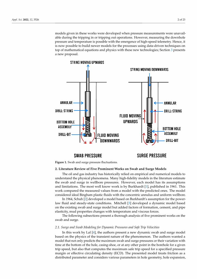
Swab and surge is a well-known problem for drilling and well construction operations.Researchers have been investigating this problem since the 19th century. Swab and surge referto pressure fluctuations due to lowering or withdrawing the pipe from the hole. See Figure 1.

Swab and surge pressure fluctuations are either positive or negative. They are positivewhen lowering down the pipe and negative when withdrawing the pipe. The intensity ofthese pressure fluctuations depends on the speed of the lowering down (tripping in) orwithdrawing the pipe out (tripping out). If the tripping speed is very high, the correspond-ing pressure fluctuation is high, and in some cases, this can be higher than the fracturepressure of the formation. This will cause fracturing the formation, partial or in some casesfull losses, and in a worst-case scenario well collapse can occur. If the tripping speed istoo low, this leads to a slow tripping operation, which is considered non-productive time(NPT), increasing the overall well budget.

The reverse of positive pressure fluctuation is also true. If the pipe is withdrawn veryfast from the hole, this will lead to negative pressure in the wellbore and well inflow andcan cause kick. In a worst-case scenario well incident or blowout can happen.

Researchers over the years have looked into swab and surge, utilizing mathematicalequations and physics to understand the phenomena. As a result, some empirical, math-ematical, and physics-based models are available for swab and surge simulations. Thispaper looks into some literature on the swab and surge in wellbore pressures. The literaturestudy presented in Section 2 presents a thorough analysis of five prominent works. The

Appl. Sci. 2022, 12, 3526. https://doi.org/10.3390/app12073526 https://www.mdpi.com/journal/applsci

Appl. Sci. 2022, 12, 3526 2 of 23

models given in these works were developed when pressure measurements were unavail-able during the tripping in or tripping out operations. However, measuring the downholepressure and temperature is possible with the emergence of high-speed telemetry. Hence, itis now possible to build newer models for the processes using data-driven techniques ontop of mathematical equations and physics with these new technologies; Section 3 presentsa new proposal.

Figure 1. Swab and surge pressure fluctuations.

2. Literature Review of Five Prominent Works on Swab and Surge Models

The oil and gas industry has historically relied on empirical and numerical models tounderstand the physical phenomena. Many high-fidelity models in the literature estimatethe swab and surge in wellbore pressures. However, each model has its assumptionsand limitations. The most well know work is by Burkhardt [1], published in 1961. Thiswork compared the measured values from a model with the predicted ones. The modelconsidered ideal Bingham plastic fluids with the concentric annulus and uniform wellbore.

In 1964, Schuh [2] developed a model based on Burkhardt’s assumption for the power-law fluid and steady-state conditions. Mitchell [3] developed a dynamic model basedon the existing swab and surge model but added factors of formation, cement, and pipeelasticity, mud properties changes with temperature and viscous forces.

The following subsections present a thorough analysis of five prominent works on theswab and surge.

2.1. Surge and Swab Modeling for Dynamic Pressures and Safe Trip Velocities

In this work by Lal [4], the authors present a new dynamic swab and surge modelbased on the physics of the transient nature of the phenomenon. The authors wanted amodel that not only predicts the maximum swab and surge pressures or their variation withtime at the bottom of the hole, casing-shoe, or at any other point in the borehole for a giventrip speed, but also that computes the maximum safe trip speed for a specified pressuremargin or effective circulating density (ECD). The presented model treats friction as adistributed parameter and considers various parameters in hole geometry, hole expansion,

Appl. Sci. 2022, 12, 3526 3 of 23

varying trip velocity, return area for tricone and diamond drill bits, plugged jets, andmud properties.

2.1.1. Lal’s Model

Unsteady transient flow in the borehole due to pipe movement generates pressuresurges that propagate at the sound velocity, C. For a given set of initial boundary conditions,the transient nature of a pipe movement in the borehole with a certain cross-section area, A,depends on the fluid density, fluid compressibility, conduit expansion ability, and friction(resistance to flow).

The model of this work [4] is shown in Equations (1) to (6). This model shows thefundamental equations for the transient pressure and average flow rate in a vertical wellwith a constant area of cross-section were obtained from the momentum balance, flowcontinuity, and equations of state.

∂p∂z

+pA

∂g∂t

+ h f(q, vp

)= 0 (1)

∂p∂t

+ s · c ∂q∂z

= 0 (2)

S = Pc/A (3)

c =√

g/ρ(α + β) (4)

∆P =1α

∂VV

(5)

∆P =1α

Ap · ∆LAh · L

(6)

This work solved the first two equations for the known initial and the boundaryconditions at the endpoints, considering every section in a borehole filled with drilling fluidand in communication with the other sections. Also, the endpoints boundary conditionswere determined from pressure variations and the flow continuity.

The impedance of surge is given by Equation (3). The sonic speed of propagation,C, is given by Equation (4). For calculating acoustic speed, C, a compressibility factor2.7× 10−6 (psi) of water at 122 deg F and 7255 psi was used. The expansibility factor forvarious conduits is derived from the theory of elasticity.

This work computed the friction pressure term by utilizing the Power-Law drillingfluid model. In addition, the frictional pressure loss term in the Power-Law model for thestatic pipe and fluid in the annulus was modified for incorporating the moving pipe effecton the average cross-section fluid speed and flow rate.

For the turbulent fluid, the Equation (1) becomes non-linear due to the nature of thefriction term. This work also employed the characteristic popular numerical technique usedfor computing problems of unsteady flow. This method essentially converts Equations (1)and (2) to ordinary differential equations while using the finite difference scheme forconverting these equations to algebraic form.

The effect of initial pressure required to break the mud gel were computed fromthe fluid compressibility. According to the definition of fluid compressibility if a fluid ofvolume is compressed by a small volume, this can result in an increase in the pressure andis given by Equation (3).

Suppose a pipe with a cross-section area, Ap, is moved a small distance ∆L, in an openhole with cross-section area, Ah, and length L, from the bottom of the pipe to the wellbore.The resulting increase in pressure ∆P due to compressing the fluid below the pipe is givenby Equation (4).

From the computed result, the model assumes that the effect of gel breaking the mudon the initial pressure is insignificant. Therefore, the initial conditions are taken as zero.

Appl. Sci. 2022, 12, 3526 4 of 23

The calculated pressures and flow rates along the fluid line (pipe moving the hole) att = ∆t are used as the initial inputs to calculate the pressures and flow rates at time t = 2∆t.This computation is continued to calculate the pressures and the flow rates at a differenttime span along the pipe and the borehole.

2.1.2. Analysis of the Work by Lal

The main feature of the work [4] is the computer program to predict the maximumswab and surge pressures, the variations of swab and surge in the time domain at thebottom wellbore, and casing when running a casing, liner, or drill pipe stand. The computerprogram also generates warnings of lost circulation for surge or influx for the swab.

This work presents the main features of the theory for the model and a computerprogram. Based on the theoretical development of the dynamic swab and surge model,the computer program has been written, tested, and validated to some extent based onlimited measured data. It simulates conditions in boreholes with fairly complex geometries,considering casing, liner, open hole, tricone or diamond bits, and the return area aroundthe bit, drill collars, special pipe, or top drill collars, and drill pipe. The computer programhas the following main features:

1. It predicts the maximum surge or swab pressure or their variation with time at thebottomhole and casing-shoe when running a casing joint, liner, or a drill pipe stand;

2. It warns about the danger of lost circulation for the surge (or kick for the swab)when the computed maximum pressure (or minimum pressure for swab) exceeds (orfalls below) the specified pressure margin or the maximum (or minimum for swab)equivalent mud weight. For each case, it computes the maximum safe trip speed inorder to avoid the lost circulation or the kick problem. These answers can be obtainedwhile running in or pulling out the pipe at various distances from the bottom ofthe hole.

Based on the computer program runs, the authors had the following conclusionsregarding swab and surge pressures:

1. The computations of swab and surge pressures based on steady-state flow are gener-ally incorrect given the unsteady nature of the flow;

2. As far as the effect of various parameters on the swab and surge pressures is concerned,these parameters can be listed, in order of their importance, as follows.

The most critical parameters are the maximum trip speed and various parameters inhole geometry, such as the size of the hole and various pipes, and the depth of the welland the relative depth at which a pipe is being run. From the given example, one may runa pipe at a higher trip speed when running at large distances from the bottom, but onemust carefully note the increase in surge pressure at the casing shoe when the pipe is closeto it. The effect of the expansion of the hole and other conduits is also significant. In thecase of the drill string, the plugging of the jet nozzles in tricone bits (or crowfoot area indiamond bits) and the constriction of the annulus return area can also significantly affectthe swab and surge pressures. Regarding the effect of mud parameters, the increase inyield value has a maximum. However, not as many preceding parameters affect the surgepressure, followed by the plastic viscosity and mud weight. The mud weight appears tohave a relatively small effect on the surge pressures.

The computer program written for the model includes almost all the significantparameters. It is user-friendly and has fast run times. It accurately predicts not only themaximum surge pressure or its time-variation at any point in the well but also computesthe safe maximum trip speed when running a casing, liner, or drill string at a given depthin the borehole.

2.2. Bottomhole Pressure Surges While Running Pipe

The work by Clark [5] suggests a method of calculating bottomhole pressure surgesdue to the movement of tubular goods in a wellbore and the use of these values in predicting

Appl. Sci. 2022, 12, 3526 5 of 23

their effect on further drilling and completion. The work explains formulas for calculatingand predicting various factors working behind the scenes during drilling and how theyare used.

This work started an investigation of pressure surges by analyzing the factors thatgo into their calculations and then developing a set of formulas that predict the pressuresurges. The work makes several assumptions in order to develop such formulas. One ofthe important assumptions is that the fluid and the borehole walls are incompressible. Thesecond assumption this work makes is that the tubing being lowered is concentric with theborehole all the time. This means the hole is perfectly engaged for its complete length.

Ormsby [6] reorganized the equations for pressure drop due to friction for the plasticfluids in steady laminar flow in the fixed boundaries developed by Beck et al. [7] from theBingham fluid model.

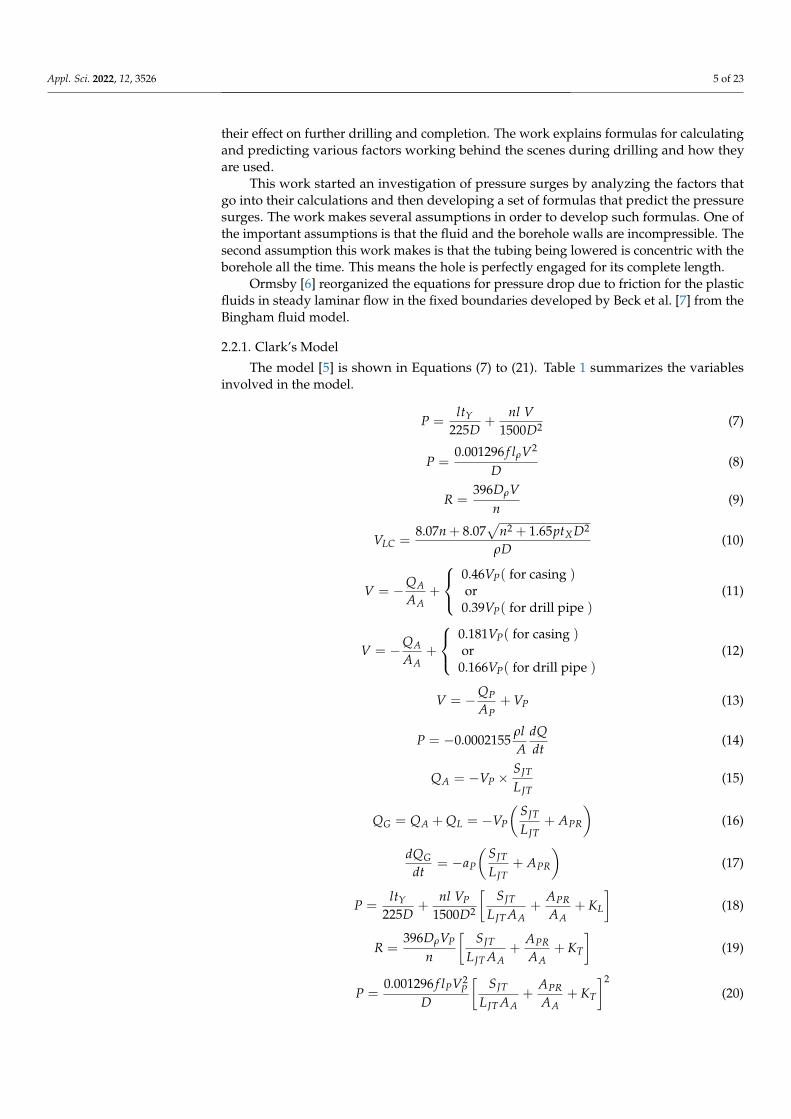
2.2.1. Clark’s Model

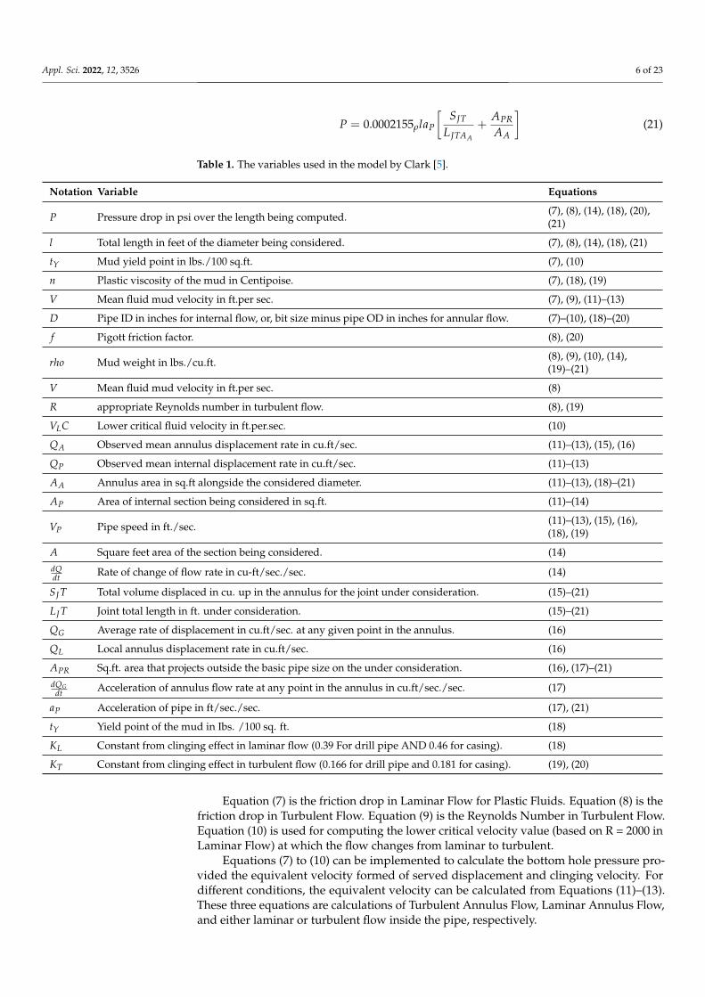
The model [5] is shown in Equations (7) to (21). Table 1 summarizes the variablesinvolved in the model.

P =ltY

225D+

nl V1500D2 (7)

P =0.001296 f lρV2

D(8)

R =396DρV

n(9)

VLC =8.07n + 8.07

√n2 + 1.65ptXD2

ρD(10)

V = −QAAA

+

0.46VP( for casing )or

0.39VP( for drill pipe )(11)

V = −QAAA

+

0.181VP( for casing )or

0.166VP( for drill pipe )(12)

V = −QPAP

+ VP (13)

P = −0.0002155ρlA

dQdt

(14)

QA = −VP ×SJT

LJT(15)

QG = QA + QL = −VP

(SJT

LJT+ APR

)(16)

dQGdt

= −aP

(SJT

LJT+ APR

)(17)

P =ltY

225D+

nl VP

1500D2

[SJT

LJT AA+

APRAA

+ KL

](18)

R =396DρVP

n

[SJT

LJT AA+

APRAA

+ KT

](19)

P =0.001296 f lPV2

PD

[SJT

LJT AA+

APRAA

+ KT

]2(20)

Appl. Sci. 2022, 12, 3526 6 of 23

P = 0.0002155ρlaP

[SJT

LJTAA

+APRAA

](21)

Table 1. The variables used in the model by Clark [5].

Notation Variable Equations

P Pressure drop in psi over the length being computed. (7), (8), (14), (18), (20),(21)

l Total length in feet of the diameter being considered. (7), (8), (14), (18), (21)

tY Mud yield point in lbs./100 sq.ft. (7), (10)

n Plastic viscosity of the mud in Centipoise. (7), (18), (19)

V Mean fluid mud velocity in ft.per sec. (7), (9), (11)–(13)

D Pipe ID in inches for internal flow, or, bit size minus pipe OD in inches for annular flow. (7)–(10), (18)–(20)

f Pigott friction factor. (8), (20)

rho Mud weight in lbs./cu.ft. (8), (9), (10), (14),(19)–(21)

V Mean fluid mud velocity in ft.per sec. (8)

R appropriate Reynolds number in turbulent flow. (8), (19)

VLC Lower critical fluid velocity in ft.per.sec. (10)

QA Observed mean annulus displacement rate in cu.ft/sec. (11)–(13), (15), (16)

QP Observed mean internal displacement rate in cu.ft/sec. (11)–(13)

AA Annulus area in sq.ft alongside the considered diameter. (11)–(13), (18)–(21)

AP Area of internal section being considered in sq.ft. (11)–(14)

VP Pipe speed in ft./sec. (11)–(13), (15), (16),(18), (19)

A Square feet area of the section being considered. (14)dQdt Rate of change of flow rate in cu-ft/sec./sec. (14)

SJ T Total volume displaced in cu. up in the annulus for the joint under consideration. (15)–(21)

LJ T Joint total length in ft. under consideration. (15)–(21)

QG Average rate of displacement in cu.ft/sec. at any given point in the annulus. (16)

QL Local annulus displacement rate in cu.ft/sec. (16)

APR Sq.ft. area that projects outside the basic pipe size on the under consideration. (16), (17)–(21)dQG

dt Acceleration of annulus flow rate at any point in the annulus in cu.ft/sec./sec. (17)

aP Acceleration of pipe in ft/sec./sec. (17), (21)

tY Yield point of the mud in Ibs. /100 sq. ft. (18)

KL Constant from clinging effect in laminar flow (0.39 For drill pipe AND 0.46 for casing). (18)

KT Constant from clinging effect in turbulent flow (0.166 for drill pipe and 0.181 for casing). (19), (20)

Equation (7) is the friction drop in Laminar Flow for Plastic Fluids. Equation (8) is thefriction drop in Turbulent Flow. Equation (9) is the Reynolds Number in Turbulent Flow.Equation (10) is used for computing the lower critical velocity value (based on R = 2000 inLaminar Flow) at which the flow changes from laminar to turbulent.

Equations (7) to (10) can be implemented to calculate the bottom hole pressure pro-vided the equivalent velocity formed of served displacement and clinging velocity. Fordifferent conditions, the equivalent velocity can be calculated from Equations (11)–(13).These three equations are calculations of Turbulent Annulus Flow, Laminar Annulus Flow,and either laminar or turbulent flow inside the pipe, respectively.

Appl. Sci. 2022, 12, 3526 7 of 23

Acceleration Pressure: The pipe goes from zero speed to a maximum speed and thenback to zero when dropping downpipe in the hole. Since the pipe movement makes the fluidmove from rest to a peak and then return to static, there must be an increase and decreasein pressure with respect to the dropping cycle. The value of these respective increase anddecrease in pressure between any two points can be calculated from Equation (14).

Conversion into Measurable Values: Due to the difficulties of measuring the fluid flowvariables, these should convert mostly the available values of speed and acceleration of thepipe. For buoyancy in an incompressible fluid, this relationship is given by Equation (15).Equation (15) is strictly not true when the float is not included in the bottom hole assembly;this allows the fluid to find its own path of minimum energy loss.

Local Displacement: Where an expanded diameter exists on a pipe string, at theselocations, there must be a movement over and above the surface-recorded displacement.This is evident, since as the projection falls, a local fluid movement must occur from theforecast to fill the gap produced behind the projection. The amount of these local fluiddisplacements is equal to the projection area multiplied by the pipe speed. Equation (16)would be used to obtain the general terms of displacement at any point in the string.

A simple derivation of this flow rate will give the fluid flow acceleration in terms ofmeasurable pipe acceleration and is given in Equation (17).

Completed Formulas For Analyzing Annulus Flow: Each flow equations can now bewritten in its final form with its components, which can be directly monitored. Equation (18)yields a loss of pressure at any given pipe velocity value due to laminar flow.

Equation (19) can be used to find the Reynolds number for finding the friction factorfor the turbulent flow. However, this should not be used for critical speed as this value isonly approximated . However, it is sufficiently accurate enough to find friction factors.

The pressure drop due to the turbulent flow at any pipe speed can be calculated withEquation (20). Finally, Equation (21) is the general equation for acceleration pressure inthe Annulus. In this equation, downward pipe movement with reference to earth is takenas positive.

2.2.2. Analysis of the Work by Clark

This work [5] also explains (using various graphs) what happens during variousdrilling in which a velocity and acceleration curve of a typical 90-foot stand of drill pipe islowered into the hole. The work concludes that drill pipe or casing velocity accelerationand deceleration can and should be minimized without markedly changing the drillingtime. Through such action, the resulting savings in “trouble” costs will pay a thousandtimes over the few dollars extra per round trip. In drilling, mud should be mixed andweighted in such a manner as to maintain the plastic viscosity and yield strength at thelowest possible value consistent with other problems. Also, during casing jobs in “tightholes”, particular care must be taken with dropping time, or displacements should berelieved by fill-up devices to prevent the bottom-hole pressure from causing excessiveamounts of damage.

This work had the following recommendations on practices to be instituted as stan-dard procedure:

1. Increase running or pulling times sufficiently to keep pressures safely above zonalhydrostatic pressure, but below the formation strength at all times;

2. Decrease the rate of acceleration or deceleration of the pipe through smoother brakehandling and earlier use of a hydromatic brake;

3. Use bottom fill devices to relieve annulus volumes by internal filling;4. Increase clearances wherever possible;5. Care should be used with projections above pipe size such as oversized drill collars

and drill pipe protectors, or improperly designed centering and scratching equipmentrun on the casing;

Appl. Sci. 2022, 12, 3526 8 of 23

6. The practice of spudding back through previously drilled formations, using highrates of pumping as well as high rates of pipe acceleration and deceleration, shoulddefinitely be controlled.

2.3. Automatic Prediction of Downhole Pressure Surges in Tripping Operations

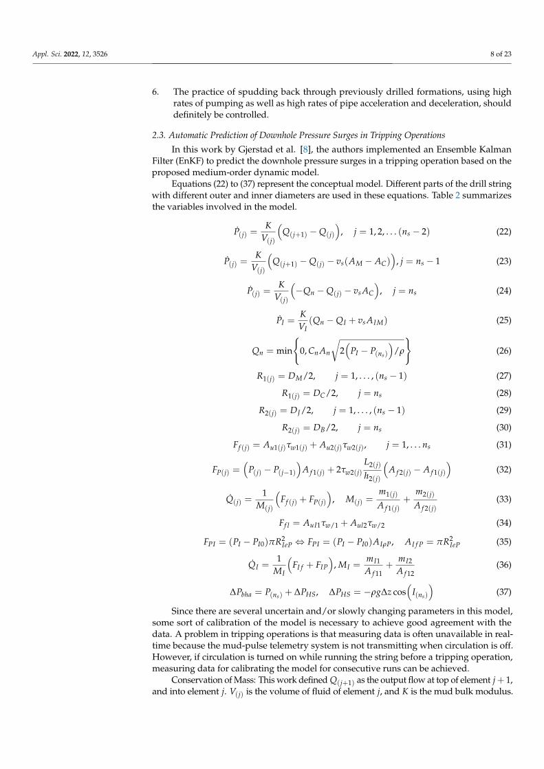
In this work by Gjerstad et al. [8], the authors implemented an Ensemble KalmanFilter (EnKF) to predict the downhole pressure surges in a tripping operation based on theproposed medium-order dynamic model.

Equations (22) to (37) represent the conceptual model. Different parts of the drill stringwith different outer and inner diameters are used in these equations. Table 2 summarizesthe variables involved in the model.

P(j) =K

V(j)

(Q(j+1) −Q(j)

), j = 1, 2, . . . (ns − 2) (22)

P(j) =K

V(j)

(Q(j+1) −Q(j) − vs(AM − AC)

), j = ns − 1 (23)

P(j) =K

V(j)

(−Qn −Q(j) − vs AC

), j = ns (24)

PI =KVI

(Qn −QI + vs AIM) (25)

Qn = min

{0, Cn An

√2(

PI − P(ns)

)/ρ

}(26)

R1(j) = DM/2, j = 1, . . . , (ns − 1) (27)

R1(j) = DC/2, j = ns (28)

R2(j) = DJ/2, j = 1, . . . , (ns − 1) (29)

R2(j) = DB/2, j = ns (30)

Ff (j) = Au1(j)τw1(j) + Au2(j)τw2(j), j = 1, . . . ns (31)

FP(j) =(

P(j) − P(j−1)

)A f 1(j) + 2τw2(j)

L2(j)

h2(j)

(A f 2(j) − A f 1(j)

)(32)

Q(j) =1

M(j)

(Ff (j) + FP(j)

), M(j) =

m1(j)

A f 1(j)+

m2(j)

A f 2(j)(33)

Ff l = AuI1τw/1 + Aul2τw/2 (34)

FPI = (PI − PI0)πR2IeP ⇔ FPI = (PI − PI0)AIρP, AI f P = πR2

IeP (35)

QI =1

MI

(FI f + FIP

), MI =

mI1

A f 11+

mI2

A f 12(36)

∆Pbha = P(ns) + ∆PHS, ∆PHS = −ρg∆z cos(

I(ns)

)(37)

Since there are several uncertain and/or slowly changing parameters in this model,some sort of calibration of the model is necessary to achieve good agreement with thedata. A problem in tripping operations is that measuring data is often unavailable in real-time because the mud-pulse telemetry system is not transmitting when circulation is off.However, if circulation is turned on while running the string before a tripping operation,measuring data for calibrating the model for consecutive runs can be achieved.

Conservation of Mass: This work defined Q(j+1) as the output flow at top of element j+ 1,and into element j. V(j) is the volume of fluid of element j, and K is the mud bulk modulus.

Appl. Sci. 2022, 12, 3526 9 of 23

AM and AC are the outer cross-section of the drill string and collars with their respectivediameters as DM and DC. The conservation of mass is presented as Equations (22) to (24).

Table 2. The variables used in the model by Gjerstad et al. [8].

Notation Variable Equations

Qn Flow through the bit nozzle. (22)–(24)

VI String inside volume. (22)–(24)

AIM String internal cross-section. (22)–(24)

ρ Mud density. (26)

An Total cross-section of all nozzles. (26)

Cn Discharge coefficient to account for unmodeled effects. (26)

Au1(j), Au2(j) The boundary surface areas. (31), (34)

τw1(j), τw2(j)Wall share stress that were calculated from respectiveradius, R1(j) or R2(j).

(31), (34)

L2(j) Length of secondary part. (32)

h2(j) Annular gap of secondary part. (32)

m1(j) Mass of main part. (33), (36)

m2(j) Mass of secondary part. (33), (36)

Because of the check valves in the string, the flow through the bit nozzle is alwaysnegative or zero. Therefore, it is given by the static expression, Equation (26).

Conservation of Momentum in the Annulus: This work divided every segment in theelements into two parts as primary and secondary part. For the main part, the radius isdefined by Equations (27) and (28). Equations (29) and (30) are for the secondary part.

The outer diameter/surface is not homogeneous as the outer diameter in the real BHAis not homogeneous. For model simplification, this work uses a normal averaging of theouter diameter of the BHA. This work separately computes the viscous friction forces ineach segment of the primary and the secondary part. Their basic equation for friction forcesis given by Equation (31).

For precise computation of the transient pressure forces on the fluid, the pressure atthe position where the cross-sectional area changes must be known. This work assumessteady-state conditions. The resultant pressure force obtained from the main part of thecross-section area was modified by an additional term dependent on the share wall stress.The resultant pressure force is given by Equation (32).

As the authors treated the volumetric flow rates as state variables, they thereforepresented the momentum as Equation (33).

Conservation of Momentum in the string: The whole surrounding wall of the drillstring moves uniformly. Therefore, the theory for calculating the viscous friction force issimpler than the annulus one. As the diameters DIM, DI J , DIC, DIB across the drill stringare not uniform, to deal the diameters non-uniformity, the authors derived an effectiveradius. This work first calculated the approximated values of the respective radii andobtained RIMFL, RI JFL, RICFL, RIBFL for laminar flow and RIMFT , RI JFT , RICFT , RIBFT forturbulent flow. Similarly, they computed the effective radii representing the secondary partof the entire volume inside the drill string.

This work expressed the friction forces as given in Equation (34).This work also computed the pressure forces by Equation (35), and the momentum

equation inside the drill string is given by Equation (36).Changes in Hydrostatic Pressure: As the BHA moves in the annulus, the pressure

sensors also follow the BHA. The authors computed the change in hydrostatic pressurecaused by the BHA movement. They left out the initial component of hydrostatic pressure

Appl. Sci. 2022, 12, 3526 10 of 23

in their computations. The change in hydrostatic pressure is given by Equation (37), inwhich the string position is give by d

dt (∆z) = vs.The Automatic Pressure Estimation: Since there are a lot of uncertainties in their model,

to achieve a good agreement with the data, it is important to have some calibration of themodel. One of the problems the authors pointed out is that during tripping operations,no real-time measurements are often available due to limitations imposed by mud pulsetelemetry, which cannot measure the pressures when the pumps are off. However, themodel can be calibrated for consecutive runs if pumps are turned on before trippingoperations. The authors employed the Ensemble Kalman Filter for the downhole pressureprediction. In addition, they computed the change in hydrostatic pressure caused bythe BHA movement. They left out the initial component of hydrostatic pressure in ourcomputations. The change in hydrostatic pressure is given by Equation (37), in which thestring position is give by d

dt (∆z) = vs.

Analysis of the Work by Gjerstad et al.

By discretization, the authors supposed that the non-linear, time-invariant system [8]can be described as:

x(t + 1) = f (x(t), u(t)) + w(t)

y(t) = h(x(t)) + v(t)

where x ∈ Rnx is the state of the system, u ∈ Rnu is the input, and y ∈ Rny is the output.The objective of their EnKF is to obtain the estimate x(t) of the true state x(t) using

the measurements y(t) so that tr(E[(x(t)− x(t))(x(t)− x(t))T]) is minimized.

This work assumed that at initial time t, there is an ensemble of N forecasted state esti-mates with random sample error. This ensemble is denoted as X f (t) =

{x f1(t), . . . , x fN (t)

}.

The obtained estimated state is:

xi(t) = x fi (t) + Ke(t)(

y(t) + vi(t)− h(

x fi (t)))

x(t) = 1/NN

∑i=1

xi(t)

A more detailed summary of the EnKF algorithm is given in the paper.During the ensemble, Kalman Filter for Automatic Parameter Estimation, the largest

uncertainties in the model were related to the viscous friction losses. Therefore, most of theparameters chosen to estimate were related to calculating frictional forces.

This work provides the algorithm for the model and a MATLAB program for sim-ulation to test the model. The authors had very limited field data, but they achievedsatisfactory estimations with their models.

2.4. Wellbore Pressure Surges by Pipe Movement

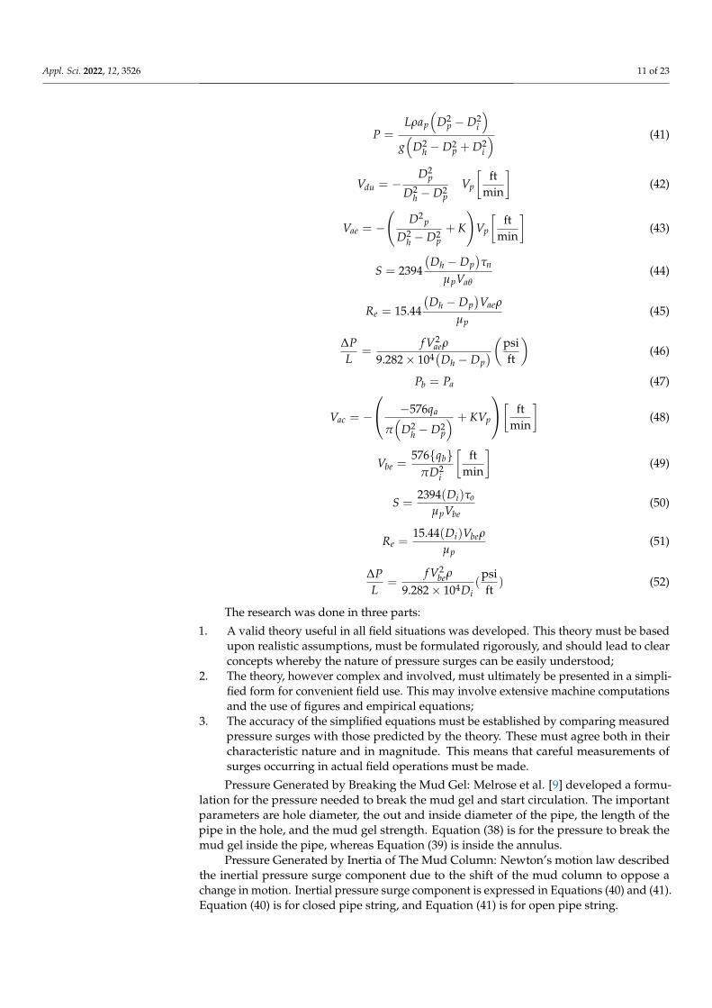
This work by Burkhardt [1] has created a theory to successfully predict the sequence andmagnitudes of these positive and negative surges and has established a basis for understandinghow they occur. The research described in this work was undertaken to supplement thatdescribed, and overcame some of the difficulties noted. The model of this work is summarizedwith Equations (38) to (52). Table 3 presents the variables involved in the model.

P =4Lζ

Di(38)

P =4Lζ

Dh − Dp(39)

P =LρapD2

p

g(

D2h − D2

p

) (40)

Appl. Sci. 2022, 12, 3526 11 of 23

P =Lρap

(D2

p − D2i

)g(

D2h − D2

p + D2i

) (41)

Vdu = −D2

p

D2h − D2

pVp

[ft

min

](42)

Vae = −(

D2p

D2h − D2

p+ K

)Vp

[ft

min

](43)

S = 2394

(Dh − Dp

)τn

µpVaθ(44)

Re = 15.44

(Dh − Dp

)Vaeρ

µp(45)

∆PL

=f V2

aeρ

9.282× 104(

Dh − Dp)(psi

ft

)(46)

Pb = Pa (47)

Vac = −

−576qa

π(

D2h − D2

p

) + KVp

[ ftmin

](48)

Vbe =576{qb}

πD2i

[ft

min

](49)

S =2394(Di)τo

µpVbe(50)

Re =15.44(Di)Vbeρ

µp(51)

∆PL

=f V2

beρ

9.282× 104Di(

psift

) (52)

The research was done in three parts:

1. A valid theory useful in all field situations was developed. This theory must be basedupon realistic assumptions, must be formulated rigorously, and should lead to clearconcepts whereby the nature of pressure surges can be easily understood;

2. The theory, however complex and involved, must ultimately be presented in a simpli-fied form for convenient field use. This may involve extensive machine computationsand the use of figures and empirical equations;

3. The accuracy of the simplified equations must be established by comparing measuredpressure surges with those predicted by the theory. These must agree both in theircharacteristic nature and in magnitude. This means that careful measurements ofsurges occurring in actual field operations must be made.

Pressure Generated by Breaking the Mud Gel: Melrose et al. [9] developed a formu-lation for the pressure needed to break the mud gel and start circulation. The importantparameters are hole diameter, the out and inside diameter of the pipe, the length of thepipe in the hole, and the mud gel strength. Equation (38) is for the pressure to break themud gel inside the pipe, whereas Equation (39) is inside the annulus.

Pressure Generated by Inertia of The Mud Column: Newton’s motion law describedthe inertial pressure surge component due to the shift of the mud column to oppose achange in motion. Inertial pressure surge component is expressed in Equations (40) and (41).Equation (40) is for closed pipe string, and Equation (41) is for open pipe string.

Appl. Sci. 2022, 12, 3526 12 of 23

Table 3. The variables used in the model by Brukhardt [1].

Notation Variable Equations

P Pressure, psi. (38), (39)

L Length of pipe section,ft. (38), (39)

ζ Mud gel strength, lb/100 f t2. (38), (39)

Di Internal diameter, in. (38), (39)

Dp Pipe outside diameter, in. (38), (39), (42)–(46),(48)

Dh Hole inside diameter, in. (38), (39), (42)–(46),(48)

ap Pipe acceleration. (40), (41)

ρ Mud density. (40), (41), (45), (46)

L Length of pipe section,ft. (40), (41)

g Acceleration of gravity. (40), (41)

Vdu Annulus competent of velocity due to displacement, ft/min. (42)

Vp Velocity of pipe, ft/min, in. (42), (43), (48)

Vae Effective annular mud velocity, ft/min. (43), (45), (48)

K Proportionality constant. (43), (48)

T0 Mud yield point, lb/100 f t2. (44)

µp Plastic viscosity, cp. (44)

Re Reynolds number. (45)∆PL Pressure gradient, psi/ft. (46)

f Friction factor. (46)

qa Mud flow in annulus measured with respect to the fixed boreholewall, f t3/min.

(48)

Vbe Effective pipe bore mud velocity, ft/min. (49)

qb Mud flow in pipe bore measured with respect to pipe walls,f t3/min.

(49)

Di Inside diameter of pipe, in. (49)

Theoretically, the viscus drag for the open and closed-end strings are similar; however,the equations are conceptual and in form differ considerably. Therefore, it is worth discussingthem separately. Closed-end pipe strings are considered in this section. Closed-end pipestrings usually have a float sub, which prevents the mud flux from the borehole to pipe string.

Determination of the Effective Annular Mud Velocity: Besides the effective velocitycomponent because of the mud clinging effect, there is also an annulus mud velocitycomponent as displacing pipe generates volumetric mudflow. This effective velocitycomponent can be determined from the relative area of the cross-section of the annulus andthe closed-end pipe, as shown in Equation (42).

The effective annular mud velocity is given by Equation (43).The mean of the effective annular mud velocity is the mud velocity that creates the

surge pressure’s viscus drag with reference to the wellbore wall.Pressure Generated Due to the Mud Flow in an Annulus: For the Bingham plastic

fluid, the plasticity for an annulus is defined by Equation (44).The Reynolds number of Bingham plastic fluid for annular flow is defined by Equation (45).By finding the friction factor using this Reynolds number, the pressure surge generated

in the annulus by moving a closed-end pipe in the borehole is given by Equation (46).

Appl. Sci. 2022, 12, 3526 13 of 23

The contribution to pressure gradients due to change in borehole or geometry of thepipe, specifically for each geometry, should be computed. Then, the total pressure wouldbe the sum of the separate component.

Viscus Drag Pressure Surges with Open Pipe Strings: The open pipe strings are defined,the strings have openings to the annulus, and the pipe bore at the string bottom, e.g., thedrill string without the float sub in the assembly or a fill-up shoe in the casing string.

A statement must be made regarding how the extra pipe borer mudflow channel isassociated with the annular mud flow path to calculate the effective annular mud velocity,creating the viscose drag pressure-surge components. The criterion utilized to characterize thisconnection was that the total pressure surge created in the pipe bore must be equal to the totalpressure surge generated in the annulus. The total pressure surge is given by Equation (47).In Equation (47), Pb is the pipe bore pressure, psi., and Pa is annulus pressure, psi.

This equality of pressure is achieved by separating the mudflow from the two path-ways in different ratios until the same pressure is created in each flow path. The ultimatepressure should be the same as the pressure that really occurred; hence, the surge pressure.

Effective Mud Velocities for Pressure-Surge Generation: The effective mean mudannulus mud velocity is the total of mud displacement and the moving pipe walls. Thus,Equation (48) presents effective annulus mud velocity.

The effective mean mud velocity in the pipe bore with reference to the pipe bore wallsis given by Equation (49).

The flow rate of the mud pipe walls qb generates pressure in the pipe bore regardlessof which is considered to be moving.

Pressure Generated in the Annulus and Pipe Bore: The pressure generated in theannulus of the open-end string is calculated the same as computed for the closed-end pipeexcept for Vae. The same method is used to calculate the pressure generated in the pipebore and the annulus. For the changed geometry, the fluid plasticity, Reynolds number,and pressure gradient equations are given in Equations (50)–(52).

The pressure gradient for each change in the diameter of the pipe bore and theannulus will vary, with the pressure created by each flow route being the total of eachdiameter change.

Analysis of the Work by Burkhardt

This work [1] presents figures for the several positive and negative pressure fluctua-tions produced when a single casing joint was lowered into a mud-filled borehole. Thiswork also presents tables that show the Mud Properties during pressure surge measure-ments during various scenarios. The comparisons listed in some tables confirm the theoryas a quantitative means of predicting pressure surges. Although several large deviationsare present in the comparisons, the deviations are generally well within the experimentalaccuracy. The agreement is especially good in the case of viscous-drag pressures, which arethe largest and therefore most important pressure peaks of the pressure-surge pattern.

The contribution of this work can be summarized as follows:

1. A quantitative, theoretical description of surge pressures generated by pipe movementin a mud-filled wellbore has been developed and verified by experimentation;

2. The theory correctly predicts the existence and magnitude of various positive andnegative peaks due to gel breaking, inertia, and viscous drag of the mud;

3. When running a drill pipe, or a casing without fill-up devices, the surge due to viscousdrag is usually the largest and, therefore, the most important;

4. Simple, approximate equations were developed to predict the viscous-drag surge,and the predictions were found to be within experimental accuracy.

2.5. Experimental Study of Swab and Surge Pressures in Horizontal and Inclined Wells

The main objective of this study by Srivastav et al. [10] is to examine the effects ofdifferent drilling parameters such as trip speed, fluid rheology, and eccentricity on swab

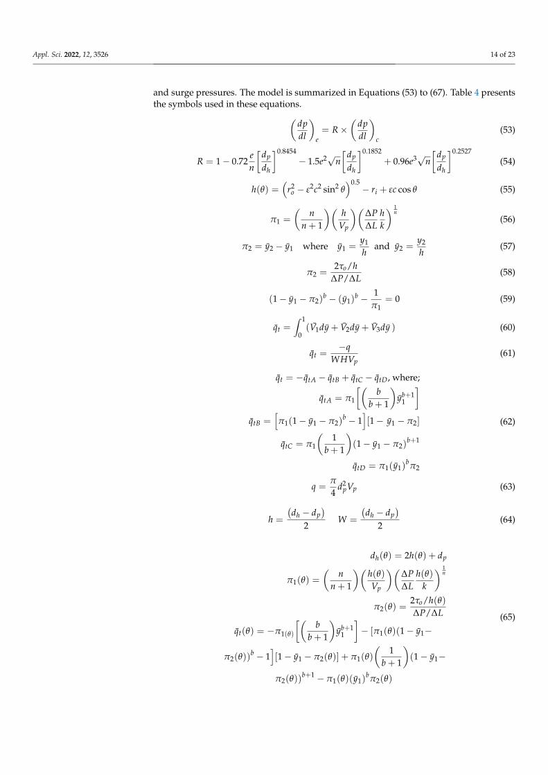
Appl. Sci. 2022, 12, 3526 14 of 23

and surge pressures. The model is summarized in Equations (53) to (67). Table 4 presentsthe symbols used in these equations.(

dpdl

)e= R×

(dpdl

)c

(53)

R = 1− 0.72en

[dp

dh

]0.8454

− 1.5e2√n[

dp

dh

]0.1852

+ 0.96e3√n[

dp

dh

]0.2527

(54)

h(θ) =(

r2o − ε2c2 sin2 θ

)0.5− ri + εc cos θ (55)

π1 =

(n

n + 1

)(h

Vp

)(∆P∆L

hk

) 1n

(56)

π2 = y2 − y1 where y1 =y1

hand y2 =

y2

h(57)

π2 =2τo/h

∆P/∆L(58)

(1− y1 − π2)b − (y1)

b − 1π1

= 0 (59)

qt =∫ 1

0(V1dy + V2dy + V3dy ) (60)

qt =−q

WHVp(61)

qt = −qtA − qtB + qtC − qtD, where;

qtA = π1

[(b

b + 1

)yb+1

1

]qtB =

[π1(1− y1 − π2)

b − 1][1− y1 − π2]

qtC = π1

(1

b + 1

)(1− y1 − π2)

b+1

qtD = π1(y1)bπ2

(62)

q =π

4d2

pVp (63)

h =

(dh − dp

)2

W =

(dh − dp

)2

(64)

dh(θ) = 2h(θ) + dp

π1(θ) =

(n

n + 1

)(h(θ)Vp

)(∆P∆L

h(θ)k

) 1n

π2(θ) =2τo/h(θ)∆P/∆L

qt(θ) = −π1(θ)

[(b

b + 1

)yb+1

1

]− [π1(θ)(1− y1−

π2(θ))b − 1

][1− y1 − π2(θ)] + π1(θ)

(1

b + 1

)(1− y1−

π2(θ))b+1 − π1(θ)(y1)

bπ2(θ)

(65)

Appl. Sci. 2022, 12, 3526 15 of 23

qtotal = 2×θ=180

∑1

qt(θ) (66)

(dpdl

)corrected

=1

K0.27ε

(dpdl

)model

(67)

Table 4. The variables used in the model by Srivastav et al. [10].

Notation Variable Equations

dp Pipe diameter. (53), (54)

dh Hole/casing diameter. (53), (54)

n Fluid behavior index. (53), (54), (56)

R Reduction factor. (53), (54)

h(θ) Element slot thickness. (55)–(58)

ro Inner radius of outer pipe. (55)

ri Outer radius of inner pipe. (55)

E Fractional eccentricity. (55)

C Radius clearance (ro − ri). (55)

Vp Pipe velocity. (56)

k Consistency Index. (56)

π2 Dimensionless plug thickness. (57)–(59), (62)

y1 Lower limit of region II. (57)

y2 Upper limit of region II. (57)

y1 Dimensionless lower boundary limit of region II. (57), (59), (62)

y2 Dimensionless upper boundary limit of region II. (57)

τo Yield stress. (58)

∆L Slot length/hole depth. (58)

∆P Pressure drop. (58)

π1 Dimensionless pressure. (59), (62)

b Constant. (59), (62)

qt dimensionless total flow rate. (60)–(62)

q Actual flow rate. (61), (63)

W Slot width. (61), (64)

Vp Pipe velocity. (61), (63)

H Slot thickness. (61), (64)

dp Pipe diameter. (63), (64)

dh Wellbore diameter. (64)

K Diameter ratio(K = dp/dh

)(67)

ε Fractional eccentricity. (67)

Haciislamoglu and Langlinais [11] developed an accurate numerical model to calcu-late the pressure loss due to the eccentricity reduction factor (R).The reduction factor isdependent on the diameter pipe ratio (K) and fluid behavior index (n).Their study alsoincludes the axial pipe and yield stress. Their study reveals that the tripping speed has aminor impact on the pressure loss for yield stress fluids. For static inner pipe, the pressure

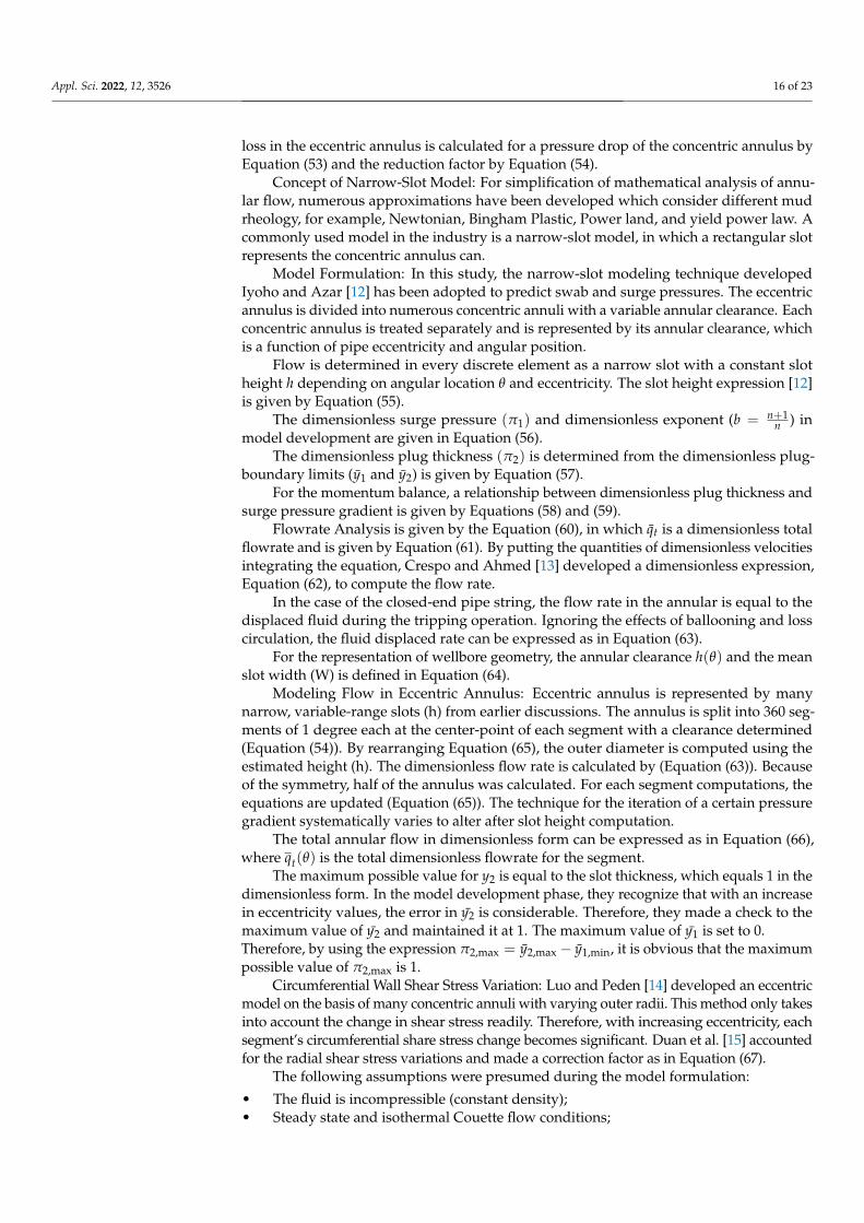
Appl. Sci. 2022, 12, 3526 16 of 23

loss in the eccentric annulus is calculated for a pressure drop of the concentric annulus byEquation (53) and the reduction factor by Equation (54).

Concept of Narrow-Slot Model: For simplification of mathematical analysis of annu-lar flow, numerous approximations have been developed which consider different mudrheology, for example, Newtonian, Bingham Plastic, Power land, and yield power law. Acommonly used model in the industry is a narrow-slot model, in which a rectangular slotrepresents the concentric annulus can.

Model Formulation: In this study, the narrow-slot modeling technique developedIyoho and Azar [12] has been adopted to predict swab and surge pressures. The eccentricannulus is divided into numerous concentric annuli with a variable annular clearance. Eachconcentric annulus is treated separately and is represented by its annular clearance, whichis a function of pipe eccentricity and angular position.

Flow is determined in every discrete element as a narrow slot with a constant slotheight h depending on angular location θ and eccentricity. The slot height expression [12]is given by Equation (55).

The dimensionless surge pressure (π1) and dimensionless exponent (b = n+1n ) in

model development are given in Equation (56).The dimensionless plug thickness (π2) is determined from the dimensionless plug-

boundary limits (y1 and y2) is given by Equation (57).For the momentum balance, a relationship between dimensionless plug thickness and

surge pressure gradient is given by Equations (58) and (59).Flowrate Analysis is given by the Equation (60), in which qt is a dimensionless total

flowrate and is given by Equation (61). By putting the quantities of dimensionless velocitiesintegrating the equation, Crespo and Ahmed [13] developed a dimensionless expression,Equation (62), to compute the flow rate.

In the case of the closed-end pipe string, the flow rate in the annular is equal to thedisplaced fluid during the tripping operation. Ignoring the effects of ballooning and losscirculation, the fluid displaced rate can be expressed as in Equation (63).

For the representation of wellbore geometry, the annular clearance h(θ) and the meanslot width (W) is defined in Equation (64).

Modeling Flow in Eccentric Annulus: Eccentric annulus is represented by manynarrow, variable-range slots (h) from earlier discussions. The annulus is split into 360 seg-ments of 1 degree each at the center-point of each segment with a clearance determined(Equation (54)). By rearranging Equation (65), the outer diameter is computed using theestimated height (h). The dimensionless flow rate is calculated by (Equation (63)). Becauseof the symmetry, half of the annulus was calculated. For each segment computations, theequations are updated (Equation (65)). The technique for the iteration of a certain pressuregradient systematically varies to alter after slot height computation.

The total annular flow in dimensionless form can be expressed as in Equation (66),where qt(θ) is the total dimensionless flowrate for the segment.

The maximum possible value for y2 is equal to the slot thickness, which equals 1 in thedimensionless form. In the model development phase, they recognize that with an increasein eccentricity values, the error in y2 is considerable. Therefore, they made a check to themaximum value of y2 and maintained it at 1. The maximum value of y1 is set to 0.Therefore, by using the expression π2,max = y2,max − y1,min, it is obvious that the maximumpossible value of π2,max is 1.

Circumferential Wall Shear Stress Variation: Luo and Peden [14] developed an eccentricmodel on the basis of many concentric annuli with varying outer radii. This method only takesinto account the change in shear stress readily. Therefore, with increasing eccentricity, eachsegment’s circumferential share stress change becomes significant. Duan et al. [15] accountedfor the radial shear stress variations and made a correction factor as in Equation (67).

The following assumptions were presumed during the model formulation:

• The fluid is incompressible (constant density);• Steady state and isothermal Couette flow conditions;

Appl. Sci. 2022, 12, 3526 17 of 23

• Laminar flow;• Drill pipe moving at a constant speed, Vp;• Negligible wall slippage effects.

Analysis of the Work by Srivastav et al.

Since the whole point of the models was to do experimental studies, the authors [10] usedan existing small-scale setup. The setup is explained in detail, and the figures compare theexperimental results with their models’ predictions. The authors then moved on to parametricstudy between two hypothetical fluids, power-law fluid, and yield-power law fluid.

The figures also show surge pressure predictions as a function of pipe velocity for bothconcentric and eccentric annulus. These figures show that the surge pressure increases withthe diameter ratio due to decreased annular clearance. The numerical model developedin this study precisely predicts swab and surge pressures, simulating downhole pressurefluctuations that occur during tripping in inclined and horizontal wells. The model utilizesthe existing variable narrow-slot approximation technique to account for pipe eccentric insurge pressure calculation.

The conclusions of this work are:

• The present model predicts swab and surge pressures of a yield power-law fluid in theeccentric annulus (i.e., eccentricity ranging from 0 to 90%) with reasonable accuracy(maximum discrepancy of 14%);

• Eccentricity has considerable effects on swab and surge pressures. Both experimen-tal and theoretical results show surge pressure reduction of up to 40% as a resultof eccentricity;

• Results show that for highly shear-thinning fluids, a small decrease in surge pressurecan considerably increase the safe tripping speed limit;

• Surge pressure predictions for the concentric and eccentric model can be consideredfor the boundary limits for the expected surge pressures. In real field conditions, dueto lateral pipe movement, the pipe does not maintain the concentric or fully eccentricgeometry throughout, resulting in surge pressure variations between these limits;

• In general, fluid rheological parameters, tripping speeds, and diameter ratios consid-erably affect the generated pressure surges.

2.6. Recent Works

Crespo et al. [16] presented a new steady-state model for power-law fluids, which in-cludes fluid and formation compressibility and pipe elasticity. Krishna et al. [17] performedlaboratory experiments to investigate the effect of centric and eccentric on the swab andsurge pressure. This work confirms that in the investigation, swab and surge pressures aregreatly affected by the tripping speed, mud properties, clearance between pipe and annular,and the eccentricity of the tube. Gjerstad et al. [18] developed a model for Herschel-Bulkleyfluids based on ordinary differential equations to predict swab and surge in real-time.

2.7. Summary of the Literature Study

Table 5 below summarizes the above models with their impact, weaknesses, assump-tions, strengths, focus, and fluid models utilized in the different models.

Appl. Sci. 2022, 12, 3526 18 of 23

Table 5. Summary of five prominent works on the swab and surge pressure model.

Model Name Impact Assumptions Strengths Weaknesses Focus Fluid Model

Srivastav et al. [10] Horizontal and extendedreach well.

Constant tripping speed.Flow approximation ineccentric annulus.

• Eccentricity effect.• Model validation

with experiments.• Good agreement

between model andexperiments.

• Constant trippingspeed.

• Experiments undercontrolledlaboratoryenvironment.

• Eccentricity effect.• Mud rheology

effect.Herschel Buckley.

Clark [5] Simple formulation. Incompressible fluid andbore hole wall.

• Pipe motion effect.• Acceleration

pressure.

• Neglected the effectof eccentricity.

• Neglected the borehole conditions.

Pressure surges causedby moving pipe inwellbore.

Bingham Plastic.

Gjerstad et al. [8]

Automatic prediction ofswab and surgepressures duringtripping operations.

Non-Newtonian fluid.

• Fast and robustautomatic downhole pressurepredictions.

• Coupling abilitywith moderncontrol for trippingspeed.

To tune the model,circulation of the wellprior to tripping.

Developing an automaticprediction of down holepressure for real-timeapplication.

Herschel Bulkley.

Burkhardt et al. [1]Theoretical prediction ofsurge and swabpressures.

Closed and open-endpipe string.

• Rigorouslyformulation forswab and surgepressures.

• Presentation offormulation withsimplified graphs.

• Measurements ofpressure pulsesgenerated bymoving pipe inwellbore.

• Computation oftransient pressuresurges due tomoving pipe inborehole.

Approximations oftheory of viscus drag bya simplified graph forfield application

Bingham Plastic.

Lal [4]

Interactive anduser-friendly swab andsurge pressurespredictions.

Friction as a “lumpedparameter”.

Non-Newtonian fluidDynamic model.

Friction as a “lumpedparameter”. Dynamic modeling. Power Law.

Appl. Sci. 2022, 12, 3526 19 of 23

3. Data-Driven Modeling in Drilling in Well Operations

Many researchers have recently made a paradigm in drilling and well operationsand implemented data-driven techniques to improve operational performance and reducerisks. Traditionally, the oil and gas industry, especially drilling, heavily relied on theanalytical modeling approach. However, recent advancements such as big data, dataanalytics, machine learning modeling, and AI modeling have tremendous value creation inother industries. Hence, the oil and gas industry and drilling are also implementing thesetechniques to create value through performance improvements and reduce risks.

The oil and gas industry’s decision-making process revolves around quantifying uncer-tainty, limiting risk, and maximizing profit, as well as speed. The ever-increasing amountof data collected due to technological advancements can drastically improve the intuitivejudgments made in numerous day-to-day operations. However, the data’s potential advan-tages can only be realized if the correct tools are used to combine various forms of data andtranslate it into valuable information that can be used to draw wise conclusions.

3.1. Applications of Data-Driven Techniques in Oil and Gas

Data-driven approaches are effective instruments for transforming information intoknowledge. Due to a lack of well-organized data, historical data has not been used ef-fectively in assessing operations. However, there is an enormous potential for turningterabytes of data into knowledge. Data-driven models have become increasingly commonlyemployed in the analysis, predictive modeling, control, and optimization of numerousprocesses due to improvements and implementation of data-driven approaches. Eventhough physics and geology are frequently included in this technique, the industry as awhole is still cautious of the adoption of data-driven methods since they are data-basedsolutions rather than traditional physics-based approaches [19].

3.2. Subsurface Characterization and Petrophysics

In the oil and gas industry, mathematical models are commonly employed. Forexample, Taner et al. [20] created a mathematical model that describes how complicatedtrace analysis is applied to seismic data and how it might be used in geologic interpretation.On the other hand, mathematical models have severe constraints and are more difficultto mimic. Therefore, several researchers in the oil and gas industry have also employeddata-driven methodologies. Specifically, reservoir management and simulation, productionand drilling optimization, real-time drilling automation, and facility maintenance are thekey application areas [21]. This section will look at some of the applications of the stateddata-driven methodologies in various industries.

Ouenes [22] investigated the usefulness of fuzzy logic and neural networks in fracturedreservoir characterization, using three phases to compare the performance of two alternativemodels. Ouenes [22] showed that by employing fuzzy curves, the influence of each modelinput on fractures can be characterized, and the factors that may have a high link withfractures can be determined [23]. Al-Anazi et al. [24] presented research that used supportvector regression (an SVM extension) to accurately estimate the porosity and permeabilityvalues for a field. Hosseini et al. [25] demonstrated how a random forest tree algorithmsupported by a naive Bayesian operation might be utilized to analyze field permeability.

For intersecting and near-well fracture corridors, Ozkaya [26] demonstrated the useof decision trees. Chamkalani et al. [27], El-Sebakhy [28], Tohidi-Hosseini [29], andAhmadi et al. [30] have used SVM and decision trees to predict gas PVT characteristics aswell as oil–gas interaction. Analyzing logs and generating missing log tracts are two of themost common artificial intelligence applications. For example, to produce a sonic log toassess over-pressured zones at the Anardarko Basin, Cranganu et al. [31] used a SupportVector Regression technique.

Akande et al. [32] created a support Vector Regression approach supported by anevolutionary algorithm to generate the best hydrocarbon estimations from logs acquiredfrom logs from a reservoir. Another use of machine learning was estimating a reservoir’s

Appl. Sci. 2022, 12, 3526 20 of 23

Total Organic Content using log data [33]. Masoudi et al. [34] created a supervisedDymanic Bayseian Network (DBN) algorithm that learned from logs to produce a modelfor identifying reservoirs without the need for user-defined cut-offs. Anifowose et al. [35]suggested an ensemble SVM approach for predicting porosity and permeability valuescomparable to the random forest tree algorithm.

3.3. Drilling

Drilling has made significant progress, particularly in risk control, regulated rateof penetrations, and so on. Ahmadi et al. [30] utilized SVM to model the rheology ofmany drilling fluids under various environmental circumstances. Cross-verification alsorevealed a strong agreement between the forecast and the test data. Fatehi et al. [36]used deposition information to construct a transductive support vector machine systemfor mapping possible drilling targets during exploration. Zhang et al. [23] developed aDynamic Bayesian Network (DBN) to efficiently analyze risk and uncertainty in controlledpressure drilling. This approach takes into account several elements to calculate uncertaintyutilizing additional probability parameters. DBN was also utilized by Al-Yami et al. [37]to create a drilling expert system based on reservoir and fluid data. Bhandari et al. [38]developed a technique to anticipate the conditions that lead to an offshore blow-out,particularly during conducted measured pressure drilling and unbalanced drilling, as wellas risk analysis. Sule et al. [39] conducted a similar study that looked at the robustnessof system controls after recreating kick circumstances used in measured pressure drilling.Chang et al. [40] also used DBN algorithms to examine emergency riser disconnectionmodules. Six disconnected module criteria linked the DBN system and the failure treeinvestigation. Cai et al. [41] used a DBN to investigate the dependability of BlowoutPreventer redundancy in deep-sea wells. Principal component analysis was utilized byKormaksson et al. [42] to find economically viable sites for new wells. Bakshi [43] developeda unique nonlinear regression model to predict shale oil well performance, includingoptimal well sites and completion parameters. Temizel et al. [44] investigated the factorsthat impact vertical and horizontal well performance in confined reservoirs.

4. Proposal for New Research on Surge and Swab Pressure Modeling

New research on swab and surge Pressure Modeling is proposed in this section, basedon the literature review. The literature in Section 2 presented a thorough analysis of fiveworks. The models given in these works were developed when pressure measurementswere unavailable during the tripping in or tripping out operations. However, with theemergence of high-speed telemetry (NOV wired drill pipe) and data while tripping tool(NOV DWT), measuring the downhole pressure and temperature is possible when trippingin or tripping out of hole [45,46]. Therefore, NOV wired drill pipe and data while trippingtool made it possible to look into swab and surge to understand the phenomena better.With these new technologies, it is now possible to build a new model for the processesusing data-driven techniques on top of mathematical equations and physics.

4.1. The Role of Sensors and Data Acquisition (Logging Data)

This section presents an overview of different sensors used to understand a well’sphysical properties, from the surface to the final depth.

The sensors and the sensor recording systems are classified into different categoriesbased on the physical attributes to be measured:

• Depth tracking sensor;• Flow in and out tracking sensors;• Measurement while drilling (MWD) and Logging-While-Drilling (LWD) tool;• Electromagnetic-Wave Resistivity (EWR) tool;• Electronic Drilling Recorder (EDR) system.

Appl. Sci. 2022, 12, 3526 21 of 23

The depth tracking sensor provides instantaneous or an average rate of penetration(ROP) based on the amount of work done by draw works or change in hydrostatic pressurein a column of water.

The flow in and out tracking sensors are used to monitor the fluid-flow rate beingapplied downhole and the flow rate coming out of the annulus; these sensors provide anearly warning of either a kick condition or a loss of circulation. The surface revolutions-per-minute (RPM), rotary torque, and hook load are obtained using Drill-monitor sensors,used for efficient drilling and minimizing downhole failures like stick-slip or stuck-pipe.Several other sensors are used to measure the drilling mud level, surface pressure, andgases present in the formation, which helps to understand downhole conditions better.

Measurement while drilling (MWD) is a type of Logging-While-Drilling (LWD), inwhich tools are encompassed in a single module in the steering tool. This tool is withthe drill string at the end of the drilling apparatus, providing wellbore position, drill bitinformation, and directional data, as well as real-time drilling information.

In the rig site software system, MWD and LWD are the most comprehensive data-acquisition systems present at the rig site. Real-time data-acquisition systems typicallyconnected to a surface and downhole sensor enable live monitoring of the rig-equipment op-eration and the well-construction process. The obtained surface measurements are stored inan electronic drilling recorder (EDR) system in the form of electronic tour-sheet applications.

4.2. The Steps Involved in New Research

With the availability of real-time drilling data, we propose developing newer modelsfor swab and surge pressures. The following steps are involved:

1. Preparing the data;2. Validating the existing models with the data and improving the model;3. Testing the new model.

Research with field data also demands the development of newer algorithms for theautomated processing of tripping in, tripping out, and the drilling data of an actual well.During the tripping in and tripping out process in drilling operations, E&P companiesare implementing the Data While Tripping tool to obtain internal, annular Pressure, andtemperature while using Pressure While Drilling and Enhance Measurement System. How-ever, Pressure While Drilling Tool and Enhance Measurement Systems are usually fromdifferent vendors, and the sensors mounted on these tools are of varying quality. Therefore,it is essential to determine the agreement between the measurements of the same variablesfrom different methods. For example, Bland Altman Plot Analysis theory, which is utilizedin health sciences [47]) could be implemented on the Pressure While Drilling and EnhanceMeasurement System measurements obtained via data while the tripping tool throughwired drill pipe telemetry system.

5. Conclusions

The paper proposes developing newer and more robust models for the swab andsurge pressures involving actual data from tripping in, tripping out, and drilling operations.Oil companies must facilitate this research by providing field data while tripping tools(e.g., NOV DWT) and wired drill pipe telemetry systems (e.g., NOV Wired Drill PipeTelemetry Network. For example, these field data could belong to one of the fields in theBarents Sea, Norway. In this way, actual field problems that are encountered relating totripping in and tripping out can be investigated, and potential data-driven solutions can bedelivered. Several researchers have implemented data-driven methodologies to find newsolutions within ROP modeling, reservoir management, drilling optimization, and dataprocessing, and have already achieved promising results.

Using field data to improve the models further develops a solid relationship betweenacademics and industry by finding new solutions to drilling and well construction oper-ations challenges. For example, in Norce—the research institution in Norway—severalprojects on drilling automation are ongoing.

Appl. Sci. 2022, 12, 3526 22 of 23

Author Contributions: Conceptualization, A.M. and R.D.; methodology, formal analysis, and in-vestigation, A.M.; validation, R.D.; writing—original draft preparation, A.M.; writing—review andediting, R.D. All authors have read and agreed to the published version of the manuscript.

Funding: This research received no external funding.

Institutional Review Board Statement: Not applicable.

Informed Consent Statement: Not applicable.

Data Availability Statement: Not applicable.

Conflicts of Interest: The authors declare no conflict of interest.

References1. Burkhardt, J. Wellbore pressure surges produced by pipe movement. J. Pet. Technol. 1961, 13, 595–605. [CrossRef]2. Schuh, F. Computer makes surge-pressure calculations useful. Oil Gas J. 1964, 31, 96.3. Mitchell, R. Dynamic surge/swab pressure predictions. SPE Drill. Eng. 1988, 3, 325–333. [CrossRef]4. Lal, M. Surge and Swab modeling for dynamic Pressures and safe trip velocities. In Proceedings of the IADC/SPE Drilling

Conference, New Orleans, LA, USA, 20–23 February 1983.5. Clark, E. Bottom-Hole Pressure Surges While Running Pipe. Pet. Eng. Int. 1955, 27, B68.6. Ormsby, G.S. Calculation and Control of Mud Presures in Drilling and Completion Operations. In Drilling and Production Practice;

OnePetro: New York, NY, USA, 1954.7. Beck, R.; Nuss, W.; Dunn, T. The Flow Properties of Drilling Muds. In Drilling and Production Practice; OnePetro: New York, NY,

USA, 1947.8. Gjerstad, K.; Sui, D.; Bjørkevoll, K.S.; Time, R.W. Automatic prediction of downhole pressure surges in tripping operations. In

Proceedings of the International Petroleum Technology Conference, European Association of Geoscientists & Engineers (IPTC2013), Beijing, China, 26–28 March 2013.

9. Melrose, J.; Savins, J.; Foster, W.; Parish, E. A practical utilization of the theory of Bingham plastic flow in stationary pipes andannuli. Trans. AIME 1958, 213, 316–324. [CrossRef]

10. Srivastav, R.; Enfis, M.; Crespo, F.; Ahmed, R.; Saasen, A.; Laget, M. Surge and swab pressures in horizontal and inclinedwells. In Proceedings of the SPE Latin America and Caribbean Petroleum Engineering Conference, Mexico City, Mexico,16–18 April 2012.

11. Haciislamoglu, M.; Langlinais, J. Effect of pipe eccentricity on surge pressures. J. Energy Resour. Technol. 1991, 113, 157–160.[CrossRef]

12. Iyoho, A.W.; Azar, J.J. An accurate slot-flow model for non-Newtonian fluid flow through eccentric annuli. Soc. Pet. Eng. J. 1981,21, 565–572. [CrossRef]

13. Crespo, F.; Aven, N.K.; Cortez, J.; Soliman, M.; Bokane, A.; Jain, S.; Deshpande, Y. Proppant distribution in multistage hydraulicfractured wells: A large-scale inside-casing investigation. In Proceedings of the SPE Hydraulic Fracturing Technology Conference,The Woodlands, TX, USA, 4–6 February 2013.

14. Luo, Y.; Peden, J. Flow of non-Newtonian fluids through eccentric annuli. SPE Prod. Eng. 1990, 5, 91–96. [CrossRef]15. Duan, M.; Miska, S.Z.; Yu, M.; Takach, N.E.; Ahmed, R.M.; Zettner, C.M. Critical conditions for effective sand-sized solids

transport in horizontal and high-angle wells. SPE Drill. Complet. 2009, 24, 229–238. [CrossRef]16. Crespo, F.; Ahmed, R.; Enfis, M.; Saasen, A.; Amani, M. Surge-and-swab pressure predictions for yield-power-law drilling fluids.

SPE Drill. Complet. 2012, 27, 574–585. [CrossRef]17. Krishna, S.; Ridha, S.; Campbell, S.; Ilyas, S.U.; Dzulkarnain, I.; Abdurrahman, M. Experimental evaluation of surge/swab

pressure in varying annular eccentricities using non-Newtonian fluid under Couette-Poiseuille flow for drilling applications.J. Pet. Sci. Eng. 2021, 206, 108982. [CrossRef]

18. Gjerstad, K.; Time, R.W. Simplified Explicit Flow Equations for Herschel-Bulkley Fluids in Couette-Poiseuille Flow—ForReal-Time Surge and Swab Modeling in Drilling. SPE J. 2015, 20, 610–627. [CrossRef]

19. Balaji, K.; Rabiei, M.; Suicmez, V.; Canbaz, C.H.; Agharzeyva, Z.; Tek, S.; Bulut, U.; Temizel, C. Status of data-driven methods andtheir applications in oil and gas industry. In Proceedings of the SPE Europec featured at 80th EAGE Conference and Exhibition,Copenhagen, Denmark, 11–14 June 2018.

20. Taner, M.T.; Koehler, F.; Sheriff, R. Complex seismic trace analysis. Geophysics 1979, 44, 1041–1063. [CrossRef]21. Holdaway, K.R. Harness Oil and Gas Big Data with Analytics: Optimize Exploration and Production with Data-Driven Models; John

Wiley & Sons: Hoboken, NJ, USA, 2014.22. Ouenes, A. Practical application of fuzzy logic and neural networks to fractured reservoir characterization. Comput. Geosci. 2000,

26, 953–962. [CrossRef]23. Zhang, L.; Wu, S.; Zheng, W.; Fan, J. A dynamic and quantitative risk assessment method with uncertainties for offshore managed

pressure drilling phases. Saf. Sci. 2018, 104, 39–54. [CrossRef]

Appl. Sci. 2022, 12, 3526 23 of 23

24. Al-Anazi, A.F.; Gates, I.D. Support vector regression to predict porosity and permeability: Effect of sample size. Comput. Geosci.2012, 39, 64–76. [CrossRef]

25. Behnoudfar, P.; Hosseini, P.; Azizi, A. Permeability determination of cores based on their apparent attributes in the Persian Gulfregion using Navie Bayesian and Random forest algorithms. J. Nat. Gas Sci. Eng. 2017, 37, 52–68. [CrossRef]

26. Ozkaya, S.I. Using probabilistic decision trees to detect fracture corridors from dynamic data in mature oil fields. SPE Reserv.Eval. Eng. 2008, 11, 1061–1070. [CrossRef]

27. Chamkalani, A.; Zendehboudi, S.; Chamkalani, R.; Lohi, A.; Elkamel, A.; Chatzis, I. Utilization of support vector machine tocalculate gas compressibility factor. Fluid Phase Equilibria 2013, 358, 189–202. [CrossRef]

28. El-Sebakhy, E.A. Forecasting PVT properties of crude oil systems based on support vector machines modeling scheme. J. Pet. Sci.Eng. 2009, 64, 25–34. [CrossRef]

29. Tohidi-Hosseini, S.M.; Hajirezaie, S.; Hashemi-Doulatabadi, M.; Hemmati-Sarapardeh, A.; Mohammadi, A.H. Toward predictionof petroleum reservoir fluids properties: A rigorous model for estimation of solution gas-oil ratio. J. Nat. Gas Sci. Eng. 2016,29, 506–516. [CrossRef]

30. Ahmadi, M.A.; Mahmoudi, B. Development of robust model to estimate gas-oil interfacial tension using least square supportvector machine: Experimental and modeling study. J. Supercrit. Fluids 2016, 107, 122–128. [CrossRef]

31. Cranganu, C.; Breaban, M. Using support vector regression to estimate sonic log distributions: A case study from the AnadarkoBasin, Oklahoma. J. Pet. Sci. Eng. 2013, 103, 1–13. [CrossRef]

32. Akande, K.O.; Owolabi, T.O.; Olatunji, S.O.; AbdulRaheem, A. A hybrid particle swarm optimization and support vectorregression model for modelling permeability prediction of hydrocarbon reservoir. J. Pet. Sci. Eng. 2017, 150, 43–53. [CrossRef]

33. Tan, M.; Song, X.; Yang, X.; Wu, Q. Support-vector-regression machine technology for total organic carbon content predictionfrom wireline logs in organic shale: A comparative study. J. Nat. Gas Sci. Eng. 2015, 26, 792–802. [CrossRef]

34. Masoudi, P.; Tokhmechi, B.; Jafari, M.A.; Zamanzadeh, S.M.; Sherkati, S. Application of Bayesian in determining productivezones by well log data in oil wells. J. Pet. Sci. Eng. 2012, 94, 47–54. [CrossRef]

35. Anifowose, F.; Labadin, J.; Abdulraheem, A. Improving the prediction of petroleum reservoir characterization with a stackedgeneralization ensemble model of support vector machines. Appl. Soft Comput. 2015, 26, 483–496. [CrossRef]

36. Fatehi, M.; Asadi, H.H. Data integration modeling applied to drill hole planning through semi-supervised learning: A case studyfrom the Dalli Cu-Au porphyry deposit in the central Iran. J. Afr. Earth Sci. 2017, 128, 147–160. [CrossRef]

37. Al-Yami, A.S.; Al-Shaarawi, A.; Al-Bahrani, H.; Wagle, V.B.; Al-Gharbi, S.; Al-Khudiri, M.B. Using Bayesian network to developdrilling expert systems. In Proceedings of the SPE Heavy Oil Conference and Exhibition, Kuwait City, Kuwait, 6–8 December 2016.

38. Bhandari, J.; Abbassi, R.; Garaniya, V.; Khan, F. Risk analysis of deepwater drilling operations using Bayesian network. J. LossPrev. Process Ind. 2015, 38, 11–23. [CrossRef]

39. Sule, I.; Khan, F.; Butt, S.; Yang, M. Kick control reliability analysis of managed pressure drilling operation. J. Loss Prev. ProcessInd. 2018, 52, 7–20. [CrossRef]

40. Chang, Y.; Chen, G.; Wu, X.; Ye, J.; Chen, B.; Xu, L. Failure probability analysis for emergency disconnect of deepwater drillingriser using Bayesian network. J. Loss Prev. Process Ind. 2018, 51, 42–53. [CrossRef]

41. Cai, B.; Liu, Y.; Liu, Z.; Tian, X.; Dong, X.; Yu, S. Using Bayesian networks in reliability evaluation for subsea blowout preventercontrol system. Reliab. Eng. Syst. Saf. 2012, 108, 32–41. [CrossRef]

42. Kormaksson, M.; Vieira, M.R.; Zadrozny, B. A data driven method for sweet spot identification in shale plays using well log data.In Proceedings of the SPE Digital Energy Conference and Exhibition, The Woodlands, TX, USA, 3–5 March 2015.

43. Bakshi, A.; Uniacke, E.; Korjani, M.; Ershaghi, I. A novel adaptive non-linear regression method to predict shale oil wellperformance based on well completions and fracturing data. In Proceedings of the SPE Western Regional Meeting, Bakersfield,CA, USA, 23–27 April 2017.

44. Temizel, C.; Aktas, S.; Kirmaci, H.; Susuz, O.; Zhu, Y.; Balaji, K.; Ranjith, R.; Tahir, S.; Aminzadeh, F.; Yegin, C. Turning Datainto Knowledge: Data-Driven Surveillance and Optimization in Mature Fields. In Proceedings of the SPE Annual TechnicalConference and Exhibition, Dubai, United Arab Emirates, 26–28 September 2016.

45. Jeffery, C.; Pink, S.; Taylor, J.; Hewlett, R. Data While Tripping DWT: Keeping the Light on Downhole. In Proceedings of the SPEAsia Pacific Oil & Gas Conference and Exhibition, Online, 17–19 November 2020.

46. Vandvik, E.; Gomez, C.; Nygård, B.; Andreassen, E.; Ulfsnes, G.Å. Annular Pressure Management-Benefits From Using Along-String Measurements in Real time While Tripping. In Proceedings of the SPE/IADC International Drilling Conference andExhibition, Online, 8–12 March 2021.

47. Dewitte, K.; Fierens, C.; Stockl, D.; Thienpont, L.M. Application of the Bland–Altman plot for interpretation of method-comparisonstudies: A critical investigation of its practice. Clin. Chem. 2002, 48, 799–801. [CrossRef]