Modeling and Computational Strategies for Optimal Oilfield ...

Carnegie Mellon UniversityResearch Showcase @ CMU

Dissertations Theses and Dissertations

5-2013

Modeling and Computational Strategies forOptimal Oilfield Development Planning underFiscal Rules and Endogenous UncertaintiesVijay GuptaCarnegie Mellon University, [email protected]

Follow this and additional works at: http://repository.cmu.edu/dissertations

This Dissertation is brought to you for free and open access by the Theses and Dissertations at Research Showcase @ CMU. It has been accepted forinclusion in Dissertations by an authorized administrator of Research Showcase @ CMU. For more information, please contact [email protected].

Recommended CitationGupta, Vijay, "Modeling and Computational Strategies for Optimal Oilfield Development Planning under Fiscal Rules andEndogenous Uncertainties" (2013). Dissertations. Paper 231.

http://repository.cmu.edu?utm_source=repository.cmu.edu%2Fdissertations%2F231&utm_medium=PDF&utm_campaign=PDFCoverPages

http://repository.cmu.edu/dissertations?utm_source=repository.cmu.edu%2Fdissertations%2F231&utm_medium=PDF&utm_campaign=PDFCoverPages

http://repository.cmu.edu/etd?utm_source=repository.cmu.edu%2Fdissertations%2F231&utm_medium=PDF&utm_campaign=PDFCoverPages

http://repository.cmu.edu/dissertations?utm_source=repository.cmu.edu%2Fdissertations%2F231&utm_medium=PDF&utm_campaign=PDFCoverPages

http://repository.cmu.edu/dissertations/231?utm_source=repository.cmu.edu%2Fdissertations%2F231&utm_medium=PDF&utm_campaign=PDFCoverPages

mailto:[email protected]

mailto:[email protected]

Modeling and Computational Strategies for Optimal Oilfield Development

Planning under Fiscal Rules and Endogenous Uncertainties

Submitted in partial fulfillment of the requirements for

the degree of

Doctor of Philosophy

in

Chemical Engineering

Vijay Gupta

B. Tech., Chemical Engineering, IIT Roorkee

Carnegie Mellon University Pittsburgh, PA

May, 2013

To my parents and siblings

i

Acknowledgments

First and foremost, I would like to express my gratitude to my advisor, Prof.

Ignacio E. Grossmann, for providing me tremendous knowledge in the area of

process systems engineering and optimization, motivation and encouragement for

an innovative thinking, and being patient. It was a wonderful experience for me to

work with him during the last five years. I would like to thank members of my

thesis committee, Professors Nikolaos Sahinidis, Erik Ydstie, Andrew Schaefer

and François Margot for their invaluable time and inputs. I would also like to

thank my mentor Bora Tarhan for all of his suggestions during the several project

meetings.

I would like to acknowledge financial support from ExxonMobil Upstream

Research Company. I would also like to express my sincere gratitude towards the

Process Control and Logistics group at Air Liquide Delaware Research and

Technology Center, and Computational Methods group at ExxonMobil Upstream

Research Company for two amazing summer internship experiences. In particular,

I would like to thank Jeffrey Arbogast, Jean André, Sujata Pathak, Jeffrey Grenda,

Rick Mifflin and Vikas Goel for being great mentors and friends during these

internships.

I am grateful to the students at CMU and visitors to the group for their

friendship and helpful discussions. Special thanks go to: Anshul Agarwal, Fengqi

You, Juan Du, Sylvain Mouret, Sebastián Terrazas, Juan Pablo Ruiz, Bruno Calfa,

Pablo Garcia Herreros, Sumit Mitra, Francisco Trespalacios, Yisu Nie, Satyajith

Amaran, Yan Zhang, Bharat Mhatre, Ricardo Lima, Pablo Marchetti, Fabricio

Oliveira, Brage Knudsen and Mariano Martin.

Finally, I would like to thank my parents, Mr. Kailash Chandra Gupta and

Mrs. Geeta Devi Gupta, and my brothers, Vishnu and Ajay, and sister, Pinky, for

all their support and love they have given me throughout my life and the

ii

motivation to accomplish what I could not have imagine. My gratitude to them is

beyond what words can express and I would like to dedicate the thesis to them.

iii

Abstract

This dissertation proposes new mixed-integer optimization models and

computational strategies for optimal offshore oil and gas field infrastructure

planning under fiscal rules of the agreements with the host government,

accounting for endogenous uncertainties in the field parameters using a stochastic

programming framework. First, a multiperiod mixed-integer nonlinear

programming (MINLP) model is proposed in Chapter 2 that incorporates field

level investment and operating decisions, and maximizes the net present value

(NPV). Two theoretical properties are proposed to remove the bilinear terms from

the model, and further converting it to an MILP approximation to solve the

problem to global optimality. Chapter 3 extends the basic deterministic model in

Chapter 2 to include complex fiscal rules maximizing total contractor’s (oil

company) share after paying royalties, profit share, etc. to the host government.

The resulting model yields improved decisions and higher profit than the previous

one. Due to the computational issues associated with the progressive (sliding

scale) fiscal terms, a tighter formulation, a relaxation scheme, and an

approximation technique are proposed. Chapter 4 presents a general multistage

stochastic MILP model for endogenous uncertainty problems where decisions

determine the timings of uncertainty realizations. To address the issue of

exponential growth of non-anticipativity (NA) constraints in the model, a new

theoretical property is identified. Moreover, three solution strategies, i.e. a k-stage

constraint strategy; a NAC relaxation strategy; and a Lagrangean decomposition

algorithm, are also proposed to solve the realistic instances and applied to process

network examples. In Chapter 5, the deterministic formulations in Chapter 2 and 3

for oilfield development are extended to a multistage stochastic programming

formulation to account for the endogenous uncertainties in field sizes, oil

deliverabilities, water-oil-ratios and gas-oil-ratios. The Lagrangean decomposition

approach from Chapter 4 is used to solve the problem, with parallel solutions of

the scenarios. To improve the quality of the dual bound during this decomposition

iv

approach, a novel partial decomposition is proposed in Chapter 6. Chapter 7

presents a method to update the multipliers during the solution of a general two-

stage stochastic MILP model, combining the idea of dual decomposition and

integer programming sensitivity analysis, and comparing it with the subgradient

method. Finally, Chapter 8 summarizes the major findings of the dissertation and

suggests future work on the subject.

v

Contents

Acknowledgments i

Abstract iii

Contents v

List of Tables xi

List of Figures xiv

1 Introduction 1

1.1 Development planning of offshore oil and gas fields ............................... 2

1.1.1 Deterministic approaches for oil and gas field

development planning ............................................................... 4

1.1.2 Incorporating complex fiscal rules ............................................. 7

1.1.3 Incorporating uncertainties in the development planning ........... 8

1.2 Stochastic Programming ....................................................................... 12

1.3 Research Objectives ............................................................................. 16

1.4 Overview of thesis ................................................................................ 18

1.4.1 Chapter 2 ................................................................................ 19

1.4.2 Chapter 3 ................................................................................ 19

1.4.3 Chapter 4 ................................................................................ 20

1.4.4 Chapter 5 ................................................................................ 20

1.4.5 Chapter 6 ................................................................................ 21

1.4.6 Chapter 7 ................................................................................ 21

1.4.7 Chapter 8 ................................................................................ 22

2 An efficient multiperiod MINLP model for optimal planning of

offshore oil and gas field infrastructure 23

2.1 Introduction .......................................................................................... 23

vi

2.2 Problem Statement................................................................................ 28

2.3 MINLP Model ...................................................................................... 29

2.4 MILP Reformulation ............................................................................ 39

2.5 Reduced MINLP and MILP models ...................................................... 42

2.6 Numerical Results ................................................................................ 44

2.6.1 Instance 1 ................................................................................ 45

2.6.2 Instance 2 ................................................................................ 48

2.6.3 Instance 3 ................................................................................ 50

2.7 Conclusions .......................................................................................... 55

3 Modeling and computational strategies for optimal development

planning of offshore oilfields under complex fiscal rules 61

3.1 Introduction .......................................................................................... 61

3.1.1 Type of Contracts .................................................................... 62

3.1.2 Type of Fiscal terms for Concessionary Systems and PSA ...... 63

3.1.3 Ringfencing Provisions ........................................................... 64

3.2 Problem Statement................................................................................ 67

3.3 Oilfield Development Planning Model .................................................. 70

3.4 Deriving Specific Contracts from the Proposed Model .......................... 81

3.5 Computational Strategies ...................................................................... 85

3.6 Numerical Results ................................................................................ 91

3.6.1 Instance 1 ................................................................................ 91

3.6.2 Instance 2 ................................................................................ 95

3.6.3 Instance 3 .............................................................................. 101

3.7 Conclusions ........................................................................................ 105

4 Solution strategies for multistage stochastic programming

with endogenous uncertainties in the planning of process networks 107

4.1 Introduction ........................................................................................ 107

4.2 Problem Statement.............................................................................. 108

4.3 Model ................................................................................................. 109

vii

4.4 Model Reduction Scheme ................................................................... 110

4.5 Reduced Models Formulation ............................................................. 113

4.6 Solution Strategies .............................................................................. 118

4.6.1 k-stage Constraint Strategy .................................................... 118

4.6.2 NAC Relaxation Strategy ...................................................... 122

4.6.3 Lagrangean Decomposition Algorithm .................................. 124

4.7 Numerical Results .............................................................................. 126

4.7.1 Example 1 ............................................................................. 126

4.7.2 Example 2 ............................................................................. 132

4.8 Conclusions ........................................................................................ 136

5 Multistage stochastic programming approach for offshore

oilfield infrastructure planning under production sharing

agreements and endogenous uncertainties 138

5.1 Introduction ........................................................................................ 138


5.2.1 Nonlinear Reservoir Profiles ................................................. 140

5.2.2 Production Sharing Agreements ............................................ 142

5.2.3 Endogenous Uncertainties ..................................................... 143

5.3 Multistage Stochastic Programming Model ......................................... 149

5.4 Compact representation of the multistage stochastic model ................. 165

5.5 Solution Approach .............................................................................. 168


5.6.1 3 Oilfield Planning Example ................................................. 170

5.6.2 5 Oilfield Planning Example ................................................. 177

5.7 Conclusions ........................................................................................ 180

6 A new decomposition algorithm for multistage stochastic programs

with endogenous uncertainties 182

6.1 Introduction ........................................................................................ 182


viii

6.3 Model ................................................................................................. 185

6.4 Conventional Lagrangean Decomposition Algorithms ........................ 188

6.4.1 Lagrangean Decomposition based on relaxing

conditional NACs (Standard approach) ................................. 189

6.4.2 Lagrangean Decomposition based on Dualizing

all the NACs ......................................................................... 192

6.5 Proposed Lagrangean Decomposition Algorithm ................................ 197

6.5.1 Formulating the Scenario Groups .......................................... 197

6.5.2 Decomposition Algorithm ..................................................... 203

6.5.3 Alternate Proposed Lagrangean Decomposition Algorithm ... 208


6.6.1 Process network planning under uncertain yield .................... 210

6.6.2 Oilfield development planning under uncertain field

parameters ............................................................................. 216

6.7 Conclusions ........................................................................................ 224

7 Improving dual bound for stochastic MILP models using

sensitivity analysis 226

7.1 Introduction ........................................................................................ 226

7.2 Two-stage Stochastic programming .................................................... 227

7.3 Lagrangean Decomposition ................................................................ 229

7.4 Integer Programming (IP) Sensitivity Analysis ................................... 231

7.4.1 Primal Analysis ..................................................................... 232

7.4.2 Dual Analysis........................................................................ 233

7.5 Application of IP Sensitivity Analysis for Multiplier Updating

in Two-stage Stochastic Programs ...................................................... 234

7.6 Proposed Lagrangean Decomposition Algorithm ................................ 237


7.7.1 Example 1 ............................................................................. 238

7.7.2 Example 2 (Dynamic Capacity Allocation Problem

(DCAP)) ............................................................................... 241

ix

7.8 Conclusions ........................................................................................ 244

8 Conclusions 247

8.1 An efficient multiperiod MINLP model for optimal planning of

offshore oil and gas field infrastructure ............................................... 247

8.2 Modeling and computational strategies for optimal development

planning of offshore oilfields under complex fiscal rules .................... 250

8.3 Solution strategies for multistage stochastic programming

with endogenous uncertainties in the planning of process networks .... 253

8.4 Multistage stochastic programming approach for offshore


agreements and endogenous uncertainties ........................................... 255

8.5 A new decomposition algorithm for multistage stochastic

programs with endogenous uncertainties ............................................. 257

8.6 Improving dual bound for stochastic MILP models using

sensitivity analysis .............................................................................. 259

8.7 Contributions of the thesis .................................................................. 260

8.8 Recommendations for future work ...................................................... 262

Appendices 267

A Derivation of the Reservoir Profiles for Model 2 from Model 1 in

Chapter 2 267

B Comparison of the models based on (GOR, WOR) and (gc, wc)

functions, i.e. Model 1 and 2, in Chapter 2 271

C Nomenclature for the Fiscal Model in Chapter 3 273

D Proof of the Propositions in Chapter 3 278

E Sliding scale fiscal terms without binary variables in Chapter 3 284

F Proposition used for the Approximate Model in Chapter 3 286

x

G Bi-level decomposition approach for the Fiscal Model in Chapter 3 287

Bibliography 290

xi

List of Tables

2.1 Comparison of the nonlinearities involved in 3 model types ................... 45

2.2 Performance of various solvers with Model 1 and 2 for Instance 1 .......... 46

2.3 Comparison of models 1, 2 and 3 with and without binary reduction ...... 47

2.4 Comparison of various models and solvers for Instance 2 ....................... 49


2.6 Comparison of various models and solvers for Instance 3 ....................... 53


3.1 Comparison of the proposed oilfield planning models............................. 79

3.2 Comparison of the proposed oilfield planning models

(detailed connections) ............................................................................. 90

3.3 Comparison of the proposed oilfield planning models

(neglecting piping investments) .............................................................. 90

3.4 Field characteristics for instance 1 .......................................................... 92

3.5 Sliding scale Contractor’s profit oil share for instance 1 ......................... 92

3.6 Optimal Installation and Drilling Schedule for instance 1 ....................... 93

3.7 Comparison of the computational performance of various models

for instance 1 .......................................................................................... 94

3.8 Computational Results for Instance 2 (Model 3F vs. Model 3RF) ........... 96

3.9 Comparison of number of tiers vs. solution time for Model 3RF ............. 98

3.10 Results for Instance 2 after using various solution strategies ................... 99

3.11 Results for Instance 2 with ringfencing provisions .................................. 99

3.12 Bi-level decomposition for Instance 2 with ringfencing provisions ....... 100

3.13 Results for Instance 3 after using various solution strategies ................. 101

3.14 Field Sizes and Ringfencing Provisions for Instance 3 .......................... 103

3.15 Fiscal data for Instance 3 with ringfencing provisions ........................... 103

3.16 Results for Instance 3 with Ringfencing provisions ............................... 103

3.17 Optimal timings of Tier activations for various Ringfences ................... 104

xii

4.1 9 Scenarios for the given example ........................................................ 115

4.2 Scenario pairs and corresponding differentiating set D(s,s’)

for the 9 scenario example .................................................................... 116

4.3 Comparison of the various solution strategies for Example 1 ................ 129

4.4 Iterations during Lagrangean Decomposition ........................................ 130

4.5 Comparison of the original and reduced models for Example 1

considering different scenarios ............................................................. 130

4.6 Reduced Model vs. NAC-Relaxation Strategy for various

scenario instances ................................................................................. 132

4.7 Comparison of the various solution strategies for Example 2 ................ 133

4.8 Iterations during Lagrangean Decomposition ........................................ 135

5.1 3 oilfield planning example, case (i) ..................................................... 171

5.2 Model statistics for the 3 oilfield example, case (i) ............................... 171

5.3 3 oilfield planning example, case (ii) .................................................... 175

5.4 Computational results for 3 oilfield example, case (ii) .......................... 175

5.5 Sliding scale contractor’s profit oil share for the 3 oilfield

example, case (iii)................................................................................. 176

5.6 Computational results for 3 oilfield example, case (iii) ......................... 176

5.7 5 oilfield planning example, case (i) ..................................................... 178

5.8 Model statistics for the 5 oilfield example, case (i) ............................... 178

5.9 Computational results for 5 oilfield example, case (i) ........................... 179

5.10 5 oilfield planning example, case (ii) .................................................... 180

5.11 Computational results for 5 oilfield example, case (ii) .......................... 180

6.1 3 Process Network Example (4 Scenarios) ............................................ 211

6.2 Model statistics for the 3 Process Network Example ............................. 211

6.3 Comparison of the various decomposition schemes for 3 Process

Network Example ................................................................................. 213

6.4 Variations in the objective function value with uncertain parameters .... 213

xiii

6.5 5 Process Network Example (4 Scenarios) ............................................ 214

6.6 Comparison of the standard vs. proposed approach for 5 process

network example ................................................................................. 215

6.7 3 Oilfield Example (4 Scenarios), case (i) ............................................. 217

6.8 Model statistics for the 3 Oilfield Example, case (i) .............................. 217

6.9 Comparison of the various decomposition schemes for oilfield

example, case (i) ................................................................................... 219

6.10 Variations in the objective function value with uncertain

parameters, case (i) ............................................................................... 219

6.11 3 Oilfield Example (4 Scenarios), case (ii) ............................................ 220


example, case(ii) ................................................................................... 221

6.13 Comparison of the decomposition schemes for oilfield example,

case (iii) and (iv) .................................................................................. 223

7.1 Model statistics (deterministic equivalent) for Example 1 instances ...... 239

7.2 Results for example 1 with 3 scenarios ................................................. 240

7.3 Model statistics (deterministic equivalent) for Example 2

(DCAP) instances ................................................................................. 242

xiv

List of Figures

1.1 Offshore oilfield infrastructure ................................................................. 2

1.2 FPSO facility ............................................................................................ 3

1.3 TLP facility .............................................................................................. 3

1.4 Tree representations for discrete uncertainties over 3 stages.................... 15

1.5 A unified framework for oilfield development planning under

complex fiscal rules and endogenous uncertainties ................................. 18

2.1 Typical offshore oilfield infrastructure representation ............................. 24

2.2 Nonlinear Reservoir Characteristics for field (F1) for 2 FPSOs

(FPSO 1 and 2) ....................................................................................... 27

2.3 Instance 1 (3 Fields, 3 FPSOs, 10 years) ................................................. 45

2.4 Instance 3 (10 Fields, 3 FPSOs, 20 years) ............................................... 50

2.5 FPSO installation and expansion schedule .............................................. 51

2.6 FPSO-field connection schedule ............................................................. 51

2.7 Well drilling schedule for fields .............................................................. 52

2.8 Total flowrates from each FPSO facility ................................................. 52

3.1 Oilfield Planning with fiscal considerations ............................................ 61

3.2 Revenue flow for a typical Production Sharing Agreement ..................... 63

3.3 Progressive profit oil share of the contractor ........................................... 64

3.4 2 Ringfences for a set of 5 Fields ............................................................ 64

3.5 Sliding scale profit oil fraction ................................................................ 76

3.6 Contractor’s share of profit oil ................................................................ 76

3.7 Instance 1 (3 Fields, 3 FPSO, 15 years, No Ringfencing) ........................ 91

3.8 Total oil flowrate for FPSO 3 ................................................................. 93

3.9 Total gas flowrate for FPSO 3 ................................................................ 93

3.10 Cumulative Oil Produced vs. Timing of Tier activation .......................... 94

3.11 Instance 2 (5 Fields, 3 FPSO, 20 years, No ringfencing) ......................... 95

xv

3.12 Optimal liquid and gas capacities of FPSO 3 facility for Instance 2 ........ 96

3.13 Optimal well drilling schedule for Instance 2 .......................................... 97

3.14 Instance 3 with 10 Fields, 3 FPSO, 20 years ......................................... 101

3.15 Optimal Solution for Instance 3 with Ringfencing provisions ............... 104

3.16 Optimal Cumulative Oil production for Instance 3 with

Ringfencing provisions ........................................................................ 105

4.1 Model Reduction Scheme for 9 scenario example ................................. 117

4.2 NAC Relaxation Strategy ..................................................................... 123

4.3 Lagrangean Decomposition algorithm .................................................. 125

4.4 Process Network Example 1 ................................................................. 127

4.5 Installation Schedule for the Process Network Example 1 ..................... 128

4.6 Comparison of constraints in Original and Reduced Models for

Example 1 considering different scenarios ............................................ 131

4.7 Cuts Added vs. Total Constraints in the Reduced Model

for NAC Relaxation Strategy ................................................................ 131

4.8 Process Network Example 2 ................................................................. 132

4.9 Optimal Solution (Example 2) .............................................................. 134

5.1 A typical offshore oilfield infrastructure representation ........................ 139

5.2 Nonlinear Reservoir Characteristics for field (F1) for 2 FPSOs

(FPSO 1 and 2) ..................................................................................... 141

5.3 Revenue flow for a typical Production Sharing Agreement ................... 142

5.4 Progressive profit oil share of the contractor ......................................... 143

5.5 Oil deliverability per well for a field under uncertainty ......................... 144

5.6 Decision-dependent scenario tree for two fields .................................... 148

5.7 Structure of a typical Multistage Stochastic Program with

Endogenous uncertainties ..................................................................... 168


5.9 3 oilfield planning example .................................................................. 171

5.10 Optimal solution for 3 oilfield example, case (i) ................................... 172

xvi

5.11 Lagrangean decomposition results for 3 oilfield example, case (i)......... 173


6.1 Structure of a typical Multistage Stochastic Program with

Endogenous uncertainties ..................................................................... 188


6.3 Lagrangean Decomposition based on relaxing conditional NACs ......... 191

6.4 Impact of conditional NACs on the scenario tree structure .................... 191

6.5 Lagrangean Decomposition based on dualizing all NACs directly ........ 194

6.6 Structure of the Reduced Model after reformulation (MLRC) ................ 195

6.7 An illustration for the 4 Scenarios and its scenario group

decomposition (top view) ..................................................................... 198

6.8 An illustration for the 4 Scenarios and its scenario group

decomposition (front view) ................................................................... 198

6.9 Asymmetric scenario group decomposition........................................... 199

6.10 2 parameters, 16 scenarios and its scenario/scenario group

decomposition ...................................................................................... 201

6.11 Decomposition of the scenario groups into subgroups ........................... 202

6.12 3 parameters, 8 scenarios and its scenario/scenario group

decomposition ...................................................................................... 203

6.13 Scenario decomposition approach in the proposed

Lagrangean Decomposition .................................................................. 206

6.14 Alternate proposed Lagrangean decomposition approach for 4

scenario problem .................................................................................. 209

6.15 3 Process Network Example ................................................................. 210

6.16 Comparison of the various decomposition schemes for 3 process

network example .................................................................................. 212

6.17 5 Process Network Example ................................................................. 213

6.18 Variations in the scenario costs vs. bound obtained for different

scenario partitions................................................................................. 215

6.19 Comparison of the standard vs. proposed approach for 5 process

xvii

network example .................................................................................... 216



example, case (i) ................................................................................... 218


example, case (ii) .................................................................................. 221


example, case (iii)................................................................................. 222


example, case (iv) ................................................................................. 223

7.1 Scenario tree for a two-stage stochastic programming ........................... 227

7.2 Decomposable MILP model structure ................................................... 228

7.3 Lagrangean Decomposition Algorithm (standard) ................................. 229

7.4 A typical branch and bound solution tree for MILP .............................. 232

7.5 Lagrangean Decomposition Algorithm (proposed) ................................ 237

7.6 Results for example 1 with 50 scenarios (Proposed vs.

Subgradient method) ............................................................................ 241

7.7 Results for example 2 (Proposed vs. Subgradient method) .................... 243

A.1 GOR profile for field (F1) and FPSO (FPSO 1) connection................... 268

A.2 gc profile for field (F1) and FPSO (FPSO 1) connection ....................... 269

B.1 GOR and gc profiles for 1 field and 2 FPSO connections ...................... 271

G.1 Bi-level Decomposition Approach for the Fiscal model with

Ringfencing provisions ......................................................................... 288

1

Chapter 1

Introduction

The development planning of offshore oil and gas field infrastructures has

received significant attention in recent years given the new discoveries of large oil

and gas reserves in the last decade around the world. These have been facilitated

by the new technologies available for exploration and production of oilfields in

remote locations that are often hundreds of miles offshore. Surprisingly, there has

been a net increase in the total oil reserves in the last decade because of these

discoveries despite increase in the total demand (BP, Statistical review Report

2011). Therefore, there is currently a strong focus on exploration and

development activities for new oil fields all around the world, specifically at

offshore locations. However, installation and operating decisions in these projects

involve very large investments that potentially can lead to large profits, but also to

losses if these decisions are not made carefully. Therefore, the goal of this thesis

is to develop efficient mixed-integer optimization models and computational

strategies for optimal development planning of offshore oil and gas field

infrastructure considering multi-field site, nonlinear reservoir profiles, complex

fiscal rules, and endogenous uncertainties in the field parameters using a

stochastic programming framework.

This chapter begins with an overview of the offshore oil and gas field

infrastructure planning problem. Then, the various approaches used in the

literature to model and solve this problem ranging from a basic deterministic

model to incorporate fiscal and uncertainty considerations. A brief review of

stochastic programming is presented with a particular focus on the endogenous

(decision-dependent) uncertainty problems. Finally, we outline the specific

2

research objectives of the work, and conclude it with a unified modeling

framework used in the thesis for this oil and gas field development problem and a

brief overview of the corresponding chapters.

1.1 Development planning of offshore oil and gas fields

The development planning of offshore oil and gas field infrastructures represents

a very critical problem since it involves multi-billion dollar investments

(Babusiaux et al., 2007). An offshore oilfield infrastructure (Figure 1.1) is usually

very complex and comprises various production facilities such as Floating

Production, Storage and Offloading (FPSO), Figure 1.2, Tension Leg platform

(TLP), Figure 1.3, and connecting pipelines to produce oil and gas from the

reserves. Each oilfield consists of a number of potential wells to be drilled using

drilling rigs, which are then connected to the facilities through pipelines to

produce oil. The produced oil is transported to the shore either though pipelines or

using large tankers.

Figure 1.1: Offshore oilfield infrastructure

3

The life cycle of a typical offshore oilfield project consists of the following

five steps:

(1) Exploration: This activity involves geological and seismic surveys

followed by exploration wells to determine the presence of oil or gas.

(2) Appraisal: It involves drilling of delineation wells to establish the size and

quality of the potential field. Preliminary development planning and

feasibility studies are also performed.

(3) Development: Following a positive appraisal phase, this phase aims at

selecting the most appropriate development plan among many alternatives.

This step involves capital-intensive investment and operating decisions that

include facility installations, drilling, sub-sea structures, etc.

(4) Production: After the facilities are built and wells are drilled, production

starts where gas or water is usually injected in the field at a later time to

enhance productivity.

(5) Abandonment: This is the last phase of an oilfield development project

and involves the decommissioning of facility installations and subsea

structures associated with the field.

Given that most of the critical investments are usually associated with the

development planning phase of the project, this thesis focuses on the key

strategic/tactical decisions during this phase of the project. The major decisions

involved in the oilfield development planning phase are the following:

(i) Selecting platforms to install and their sizes

Figure 1.2: FPSO facility Figure 1.3: TLP facility

4

(ii) Deciding which fields to develop and what should be the order to develop

them

(iii) Deciding which wells and how many are to be drilled in the fields and in

what sequence

(iv) Deciding which fields are to be connected to which facility

(v) Determining how much oil and gas to produce from each field

Therefore, there are a very large number of alternatives that are available to

develop a particular field or group of fields. However, these decisions should

account for the physical and practical considerations, such as the following: a

field can only be developed if a corresponding facility is present; nonlinear

profiles of the reservoir that are obtained from reservoir simulators (e.g.

ECLIPSE) to predict the actual flowrates of oil, water and gas from each field;

limitation on the number of wells that can be drilled each year due to availability

of the drilling rigs; and long-term planning horizon that is the characteristic of

these projects. Therefore, optimal investment and operating decisions are essential

for this problem to ensure the highest return on the investments over the time

horizon considered. By including all the considerations described here in an

optimization model, this leads to a large-scale multiperiod mixed-integer

nonlinear programming (MINLP) problem that is difficult to solve to global

optimality. The extension of this model to the cases where we explicitly consider

the fiscal rules with the host government and the uncertainties can further lead to

a very complex problem to model and solve.

In the next sub-sections we briefly review the various approaches used in the

literature to address this problem either using a deterministic formulation or a

stochastic one.

1.1.1 Deterministic approaches for oil and gas field development planning

The oilfield development planning has traditionally been modeled as LP (Lee and

Aranofsky, 1958; and Aronofsky and Williams, 1962) or MILP (Frair, 1973)

models under certain assumptions to make them computationally tractable.

Simultaneous optimization of the investment and operating decisions has been

addressed in Bohannon (1970), Sullivan (1982) and Haugland et al. (1988) using

5

MILP formulations with different levels of details. Behrenbruch (1993)

emphasized the need to consider a correct geological model and to incorporate

flexibility into the decision process for an oilfield development project.

Iyer et al. (1998) proposed a multiperiod MILP model for optimal planning

and scheduling of offshore oilfield infrastructure investment and operations. The

model considers the facility allocation, production planning, and scheduling

within a single model and incorporates the reservoir performance, surface

pressure constraints, and oil rig resource constraints. To solve the resulting large-

scale problem, the nonlinear reservoir performance equations are approximated

through piecewise linear approximations. As the model considers the performance

of each individual well, it becomes expensive to solve for realistic multi-field

sites. Moreover, the flow rate of water was not considered explicitly for facility

capacity calculations.

Van den Heever and Grossmann (2000) extended the work of Iyer et al.

(1998) and proposed a multiperiod generalized disjunctive programming model

for oil field infrastructure planning for which they developed a bilevel

decomposition method. As opposed to Iyer and Grossmann (1998), they explicitly

incorporated a nonlinear reservoir model into the formulation but did not consider

the drill-rig limitations.

Grothey and McKinnon (2000) addressed an operational planning problem

using an MINLP formulation where gas has to be injected into a network of low

pressure oil wells to induce flow from these wells. Lagrangean decomposition and

Benders decomposition algorithms were proposed for the efficient solution of the

model. Kosmidis et al. (2002) considered a production system for oil and gas

consisting of a reservoir with several wells, headers and separators. The authors

presented a mixed integer dynamic optimization model and an efficient

approximation solution strategy for this system.

Barnes et al. (2002) optimized the production capacity of a platform and the

drilling decisions for wells associated with this platform. The authors addressed

the problem by solving a sequence of MILPs. Ortiz-Gomez et al. (2002) presented

three mixed-integer multiperiod optimization models of varying complexity for

6

the oil production planning. The problem considers fixed topology and is

concerned with the decisions involving the oil production profiles and

operation/shut in times of the wells in each time period assuming nonlinear

reservoir behavior.

Lin and Floudas (2003) considered the long-term investment and operations

planning of the integrated gas field site. A continuous-time modeling and

optimization approach was proposed introducing the concept of event points and

allowing the well platforms to come online at potentially any time within the

planning horizon. A two-level solution framework was proposed to solve the

resulting MINLP problems which showed that the continuous time approach can

reduce the computational efforts substantially and solve problems that were

intractable for the discrete-time model.

Kosmidis et al. (2005) presented a mixed integer nonlinear (MINLP) model

for the daily well scheduling in petroleum fields, where the nonlinear reservoir

behavior, the multiphase flow in wells and constraints from the surface facilities

were simultaneously considered. The authors also proposed a solution strategy

involving logic constraints, piecewise linear approximations of each well model

and an outer approximation based algorithm. Results showed an increase in oil

production of up to 10% compared to typical heuristic rules widely applied in

practice.

Carvalho and Pinto (2006a) considered an MILP formulation for oilfield

planning based on the model developed by Tsarbopoulou (2000), and proposed a

bilevel decomposition algorithm for solving large-scale problems where the

master problem determines the assignment of platforms to wells and a planning

subproblem calculates the timing for the fixed assignments. The work was further

extended by Carvalho and Pinto (2006b) to consider multiple reservoirs within the

model.

Barnes et al. (2007) addressed the optimal design and operational

management of offshore oil fields where at the design stage optimal production

capacity of a main field was determined with an adjacent satellite field and a well

drilling schedule. The problem was formulated as an MILP model. Continuous

7

variables involved individual well, jacket and topsides costs, whereas binary

variables were used to select individual wells within a defined field grid. An

MINLP model was proposed for the operational management to model the

pressure drops in pipes and wells for multiphase flow. Non-linear cost equations

were derived for the production costs of each well accounting for the length, the

production rate and their maintenance. Operational decisions included the oil

flowrates, the operation/shut-in for each well and the pressures for each point in

the piping network.

Gunnerud and Foss (2010) considered the real-time optimization of oil

production systems with a decentralized structure and modeled nonlinearities with

piecewise linear approximations, resulting in an MILP model. The Lagrange

relaxation and Dantzig–Wolfe decomposition methods were studied on a semi-

realistic model of the Troll west oil rim in Norway, which showed that both

approaches offers an interesting option to solve the complex oil production

systems as compared to the fullspace method.

1.1.2 Incorporating complex fiscal rules

The major limitation with the above approaches in the oilfield development

planning is that they do not consider the fiscal rules explicitly in the optimization

model that are associated to these fields, and mostly rely on the simple net present

value (NPV) as an objective function. Therefore, the models with these objectives

may yield the solutions that are very optimistic, which can in fact be suboptimal

after considering the impact of fiscal terms. Bagajewicz (2008) discussed the

merits and limitations of using NPV in the investment planning problems and

pointed out that additional consideration and procedures are needed for these

problems, e.g. return on investments, to make the better decisions. Laínez et al.

(2009) emphasizes that enterprise-wide decision problems must be formulated

with realistic detail, not just in the technical aspects, but also in the financial

components in order to generate solutions that are of value to an enterprise. This

requires systematically incorporating supplier/buyer options contracts within the

framework of supply-chain problems.

8

In the context of oilfield planning, fiscal rules of the agreements between the

oil company (contractor) and the host government, e.g. production sharing

contracts, usually determine the share of each of these entities in the total oil

production or gross revenues and the timing of these payments. Hence, including

fiscal considerations as part of the oilfield development problem can significantly

impact the optimal decisions and revenue flows over the planning horizon, as a

large fraction of the total oil produced is paid as royalties, profit share, etc. The

models and solutions approaches in the literature that consider the fiscal rules

within oilfield infrastructure planning are either very specific or simplified. Van

den Heever et al. (2000) and Van den Heever and Grossmann (2001) considered

optimizing the complex economic objectives including royalties, tariffs, and taxes

for the multiple gas field site where the schedule for the drilling of wells was

predetermined as a function of the timing of the installation of the well platform.

Moreover, the fiscal rules presented were specific to the gas field site considered,

but not in general form. Based on a continuous time formulation for gas field

development with complex economics of similar nature as Van den Heever and

Grossmann (2001), Lin and Floudas (2003) proposed an MINLP model and

solved it with a two-stage algorithm. Approaches based on simulation (Blake and

Roberts, 2006) and meta-modeling (Kaiser and Pulsipher, 2004) have also been

considered for the analysis of the different fiscal terms. However, the papers that

address the mathematical programming models and solution approaches for the

oilfield investments and operations with fiscal considerations are still very

limited.

1.1.3 Incorporating uncertainties in the development planning

In the literature work described above, one of the major assumptions is that there

is no uncertainty in the model parameters, which in practice is generally not true.

Although limited, there has been some work that accounts for uncertainty in the

problem of optimal development of oil and/or gas fields. Haugen (1996) proposed

a single parameter representation for uncertainty in the size of reserves and

incorporates it into a stochastic dynamic programming model for scheduling of oil

fields. However, only decisions related to the scheduling of fields were

9

considered. Meister et al. (1996) presented a model to derive exploration and

production strategies for one field under uncertainty in reserves and future oil

prices. The model was analyzed using stochastic control techniques.

Jonsbraten (1998a) addressed the oilfield development planning problem

under oil price uncertainty using an MILP formulation that was solved with a

progressive hedging algorithm. Aseeri et al. (2004) introduced uncertainty in the

oil prices and well productivity indexes, financial risk management, and

budgeting constraints into the model proposed by Iyer and Grossmann (1998), and

solved the resulting stochastic model using a sampling average approximation

algorithm.

Jonsbraten (1998b) presented an implicit enumeration algorithm for the

sequencing of oil wells under uncertainty in the size and quality of oil reserves.

The author uses a Bayesian approach to represent the resolution of uncertainty

with investments. The paper considers investment and operation decisions only

for one field. Lund (2000) addressed a stochastic dynamic programming model

for evaluating the value of flexibility in offshore development projects under

uncertainty in future oil prices and in the reserves of one field using simplified

descriptions of the main variables.

Cullick et al. (2003) proposed a model based on the integration of a global

optimization search algorithm, a finite-difference reservoir simulation, and

economics. In the solution algorithm, new decision variables were generated

using meta-heuristics, and uncertainties were handled through simulations for

fixed design variables. They presented examples having multiple oil fields with

uncertainties in the reservoir volume, fluid quality, deliverability, and costs. Few

other papers, (Begg et al., 2001; Zabalza-Mezghani et al., 2004; Bailey et al.,

2005; and Cullick et al., 2007), have also used a combination of reservoir

modeling, economics and decision making under uncertainty through simulation-

optimization frameworks.

Ulstein et al. (2007) addressed the tactical planning of petroleum production

that involves regulation of production levels from wells, splitting of production

flows into oil and gas products, further processing of gas and transportation in a

10

pipeline network. The model was solved for different cases with demand

variations, quality constraints, and system breakdowns.

Elgsæter et al. (2010) proposed a structured approach to optimize offshore

oil and gas production with uncertain models that iteratively updates setpoints,

while documenting the benefits of each proposed setpoint change through

excitation planning and result analysis. The approach is able to realize a

significant portion of the available profit potential, while ensuring feasibility

despite large initial model uncertainty.

However, most of these works either consider the very limited flexibility in

the investment and operating decisions, or handle the uncertainty in an ad-hoc

manner. Stochastic programming provides a systematic framework to model

problems that require decision-making in the presence of uncertainty by taking

uncertainty into account of one or more parameters in terms of probability

distribution functions, (Birge and Louveaux, 1997). The concept of recourse

action in the future, and availability of probability distribution in the context of

oilfield development planning problems, makes it one of the most suitable

candidates to address uncertainty. Moreover, extremely conservative decisions are

usually ignored in the solution utilizing the probability information given the

potential of high expected profits in the case of favorable outcomes.

In the context of stochastic programming, Goel and Grossmann (2004)

considered a gas field development problem under uncertainty in the size and

quality of reserves where decisions on the timing of field drilling were assumed to

yield an immediate resolution of the uncertainty, i.e. the problem involves

decision-dependent uncertainty as discussed in Jonsbraten et al. (1998); Goel and

Grossmann (2006); and Gupta and Grossmann (2011a). Linear reservoir models,

which can provide a reasonable approximation for gas fields, were used. In their

solution strategy, the authors used a relaxation problem to predict upper bounds,

and solved multistage stochastic programs for a fixed scenario tree for finding

lower bounds. Goel et al. (2006) later proposed the theoretical conditions to

reduce the number of non-anticipativity constraints in the model. The authors also

developed a branch and bound algorithm for solving the corresponding

11

disjunctive/mixed-integer programming model where lower bounds were

generated by Lagrangean duality. The proposed decomposition strategy relies on

relaxing the disjunctions and logic constraints for the conditional non-

anticipativity constraints while dualizing the initial ones at the root node. Ettehad

et al. (2011) presented a case study for the development planning of an offshore

gas field under uncertainty optimizing facility size, well counts, compression

power and production policy. A two-stage stochastic programming model was

developed to investigate the impact of uncertainties in original gas in place and

inter-compartment transmissibility. Results of two solution methods, optimization

with Monte Carlo sampling and stochastic programming, were compared which

showed that the stochastic programming approach is more efficient. The models

were also used in a value of information (VOI) analysis.

Moreover, the gradual uncertainty reduction has also been addressed for

problems in this class. Stensland and Tjøstheim (1991) have worked on a discrete

time problem for finding optimal decisions with uncertainty reduction over time

and applied their approach to oil production. These authors expressed the

uncertainty in terms of a number of production scenarios. Their main contribution

was combining production scenarios and uncertainty reduction effectively for

making optimal decisions. Dias (2002) presented four propositions to characterize

technical uncertainty and the concept of revelation towards the true value of the

variable. These four propositions, based on the theory of conditional expectations,

are employed to model technical uncertainty.

Tarhan et al. (2009) addressed the planning of offshore oil field

infrastructure involving endogenous uncertainty in the initial maximum oil

flowrate, recoverable oil volume, and water breakthrough time of the reservoir,

where decisions affect the resolution of these uncertainties. The authors extend

the work of Goel and Grossmann (2004) and Goel et al. (2006) but with three

major differences: (a) The model focuses on a single field consisting of several

reservoirs rather than multiple fields but more detailed decisions are considered.

(b) Nonlinear, rather than linear, reservoir models are considered. (c) The

resolution of uncertainty is gradual over time instead of being resolved

12

immediately. The authors also developed a multistage stochastic programming

framework that was modeled as a disjunctive/mixed-integer nonlinear

programming model consisting of individual non-convex MINLP subproblems

connected to each other through initial and conditional non-anticipativity

constraints. A duality-based branch and bound algorithm was proposed taking

advantage of the problem structure and globally optimizing each scenario problem

independently. An improved solution approach was also proposed that combines

global optimization and outer-approximation to optimize the investment and

operations decisions (Tarhan et al., 2011). However, it considers either gas/water

or oil/water components for single field and single reservoir at a detailed level.

Hence, realistic multi-field site instances can be expensive to solve with this

model.

In the next section we briefly outline the basic elements of the stochastic

programming that will be used as a modeling framework in this thesis.

1.2 Stochastic Programming

A stochastic program is a mathematical program in which some of the parameters

defining a problem instance are random (e.g. uncertain reservoir size, product

demand, yields, prices). In general, multiperiod industrial planning, scheduling,

supply-chain etc. problems under uncertainty are formulated as stochastic

programs since it allows to incorporate probability distribution of the uncertain

parameters explicitly into the model while making investment and operating

decisions, and provides an opportunity to take corrective actions in the future

(recourse) based on the actual outcomes (see Ierapetritou and Pistikopoulos, 1994;

Clay and Grossmann, 1997; Iyer and Grossmann, 1998; Schultz, 2003; Ahmed

and Garcia, 2003; Sahinidis, 2004; Ahmed et al. 2004; Li and Ierapetritou, 2012).

This area is receiving increasing attention given the limitations of deterministic

models.

Discrete probability distributions of the uncertain parameters are widely

considered to represent uncertainty in terms of the scenarios where a scenario is

given by the combination of the realization of the uncertain parameters.

13

Depending on the number of decision stages involved in the model, the stochastic

program corresponds to either a two-stage or a multistage problem. The main idea

behind two-stage stochastic programming is that we make some decisions (stage

1) here and now based on not knowing the future outcomes of the uncertain

parameters, while the rest of the decisions are stage-2 (recourse actions) decisions

that are made after uncertainty in those parameters is revealed. In this work, we

focus on more general multistage stochastic programming models where the

uncertain parameters are revealed sequentially, i.e. in multiple stages (time

periods), and the decision-maker can take corrective actions over a sequence of

the stages. In the two-stage and multistage case the cost of the decisions and the

expected cost of the recourse actions are optimized.

Based on the type of uncertain parameters involved in the problem,

stochastic programming models can be classified into two broad categories

(Jonsbraten, 1998b): exogenous uncertainty where stochastic processes are

independent of decisions that are taken (e.g. demands, prices), and endogenous

uncertainty where stochastic processes are affected by these decisions (e.g.

reservoir size and its quality). In the process systems area, Ierapetritou and

Pistikopoulos (1994), Clay and Grossmann (1997) and Iyer and Grossmann

(1998) solved various production planning problems that considered exogenous

uncertainty and formulated as the two-stage stochastic programs. Furthermore,

detailed reviews of previous work on problems with exogenous uncertainty can be

found in Schultz (2003) and Sahinidis (2004). However, a number of planning

problems involving very large investments at an early stage of the project have

endogenous (technical) uncertainty that is at-least comparable if not greater than

the exogenous (market) uncertainty. In such cases, it is essential to incorporate

endogenous uncertain parameters while making the investment decisions since it

can have a large impact on the overall project profitability.

In the context of endogenous uncertainty, our decisions can affect the

stochastic processes in two different ways (Goel and Grossmann, 2006): either

they can alter the probability distributions (type 1) (see Viswanath et al., 2004;

and Held and Woodruff, 2005), or they can determine the timing when

14

uncertainties in the parameters are resolved (type 2) (see Goel et al., 2006; Tarhan

et al., 2009). Surprisingly, these problems have received relatively little attention

in the literature despite their practical importance. Pflug (1990) addressed

endogenous uncertainty problems in the context of discrete event dynamic

systems where the underlying stochastic process depends on the optimization

decisions. Jonsbraten et al. (1998) proposed an implicit enumeration algorithm for

the problems in this class where decisions that affect the uncertain parameter

values are made at the first stage. Ahmed (2000) presented several examples

having decision dependent uncertainties that were formulated as MILP problems

and solved by LP-based branch and bound algorithms. Moreover, Viswanath et al.

(2004) and Held and Woodruff (2005) addressed the endogenous uncertainty

problems where decisions can alter the probability distributions.

There are multiple sources of uncertainty in the oil and gas field

development problem as can be seen from the literature work afore-mentioned.

The market price of oil/gas, quantity and quality of reserves at a field are the most

important sources of the uncertainty in this context. The uncertainty in oil prices

is influenced by the political, economic or other market factors and it belongs to

the exogenous uncertainty problems. The uncertainty in the reserves on the other

hand, is linked to the accuracy of the reservoir data (technical uncertainty). While

the existence of oil and gas at a field is indicated by seismic surveys and

preliminary exploratory tests, the actual amount of oil in a field, and the

efficiency of extracting the oil will only be known after capital investment has

been made at the field (Goel and Grossmann, 2004), i.e. endogenous uncertainty.

Both, the price of oil and the quality of reserves directly affect the overall

profitability of a project, and hence it is important to consider the impact of these

uncertainties when formulating the decision policy. However, due to the

significant computational challenge in this thesis we only address the uncertainty

in the field parameters where timing of uncertainty realizations is decision-

dependent. In particular, we focus on the type 2 of endogenous uncertainty where

the decisions are used to gain more information, and resolve uncertainty either

immediately or in a gradual manner. Therefore, the resulting scenario tree is

15

decision-dependent that requires modeling a superstructure of all possible

scenario trees that can occur based on the timing of the decisions (see Goel et al.,

2006; Tarhan et al., 2009).

Specifically, to address the stochastic programming problem under

consideration, we assume in this thesis that the uncertain parameters follow

discrete probability distributions and that the planning horizon consists of a fixed

number of time periods that correspond to decision points. Using these two

assumptions, the stochastic process can be represented with scenario trees. In a

scenario tree (Figure 1.4-a) each node represents a possible state of the system at

a given time period. Each arc represents the possible transition from one state in

time period t to another state in time period t+1, where each state is associated

with the probabilistic outcome of a given uncertain parameter. A path from the

root node to a leaf node represents a scenario.

An alternative representation of the scenario tree was proposed by

Ruszczynski (1997) where each scenario is represented by a set of unique nodes

(Figure 1.4-b). The horizontal lines connecting nodes in time period t mean that

nodes are identical as they have the same information and those scenarios are said

to be indistinguishable in that time period. These horizontal lines correspond to

the non-anticipativity (NA) constraints in the model that link different scenarios

and prevent the problem from being amenable to decomposition. In this work,

since we focus on multistage stochastic programming (MSSP) problems with

endogenous uncertainty where the structure of scenario tree is decision-

(a) Standard Scenario Tree with uncertain parameters θ1 and θ2 (b) Alternative Scenario Tree

θ2=2 θ2=1 θ1=1

θ1=2 θ1=1

3 4 1, 2

t=1

t=2

2

t=3

1 2 3 4

θ2=2 θ2=1

θ1=2 θ1=2 θ1=1

θ1=1

θ1=1

θ1=1

Figure 1.4: Tree representations for discrete uncertainties over 3 stages

16

dependent, we use the above alternative scenario tree representation to model

these problems effectively.

In addition to the oil and gas field development problems under endogenous

uncertainties (type 2) as described in the previous section (Goel and Grossmann,

2004; Goel et al., 2006; and Tarhan et al., 2009), there are few other practical

applications that have been addressed. In particular, Tarhan and Grossmann

(2008) applied endogenous uncertainty in the synthesis of process networks with

uncertain yields, and used gradual uncertainty resolution in the model. Solak

(2007) considered the project portfolio optimization problem that deals with the

selection of research and development projects and determination of optimal

resource allocations under decision dependent uncertainty where uncertainty is

resolved gradually. The author used the sample average approximation method

for solving the problem, where the sample problems were solved through

Lagrangean relaxation and heuristics. Boland et al. (2008) addressed the open pit

mine production scheduling problem considering endogenous uncertainty in the

total amount of rock and metal contained in it, where the excavation decisions

resolve this uncertainty. These authors also compared the fullspace results for this

mine-scheduling problem with the one where non-anticipativity constraints were

included as the ‘lazy constraints’ during the solution. Colvin and Maravelias

(2008, 2010) presented several theoretical properties, specifically for the problem

of scheduling of clinical trials having uncertain outcomes in the pharmaceutical

R&D pipeline, and developed a branch-and-cut framework to solve these MSSP

problems with endogenous uncertainty under the assumption that only few non-

anticipativity constraints be active at the optimal solution.

1.3 Research Objectives

Following are the major objectives of this thesis:

1. Develop an efficient deterministic model for offshore oil and gas field

development planning considering multiple fields, facility expansions in

the future, lead times for facility installation and expansions, individual

17

oil, water and gas flowrates, drilling rig limitations, with the objective to

maximize the net present value for the given planning horizon

2. Extend the simple NPV based deterministic oilfield planning model to

include general complex fiscal rules such as the ones in production sharing

agreements

3. Develop reformulation, approximation and decomposition based

approaches to improve the computational efficiency of the oilfield model

with fiscal rules

4. Apply these deterministic models with/without fiscal contracts and

computational strategies to realistic oilfield development planning

examples

5. Formulate a general multistage stochastic mixed-integer linear

programming model for addressing endogenous uncertainties where the

optimization decisions affect the timing when uncertainties in the

parameters are resolved

6. Develop model reduction approaches and solution strategies to overcome

the computational expense of the above multistage stochastic model

7. Apply these multistage stochastic model and solution strategies to the

process network planning problem under uncertain yields, and to the

oilfield development planning under uncertain field parameters

with/without fiscal contracts

8. Develop and implement a new Lagrangean decomposition algorithm based

on grouping of the scenarios for efficiently solving general multistage

stochastic programs under endogenous uncertainties, and apply it to

process network and oilfield planning examples to compare it with the

standard approaches

9. Develop a method for improving the dual bound generated during the

solution of a stochastic mixed-integer linear programming model using the

dual decomposition and integer programming sensitivity analysis, and

benchmark the results against the standard subgradient method

18

1.4 Overview of thesis

Figure 1.5: A unified framework for oilfield development planning under

complex fiscal rules and endogenous uncertainties

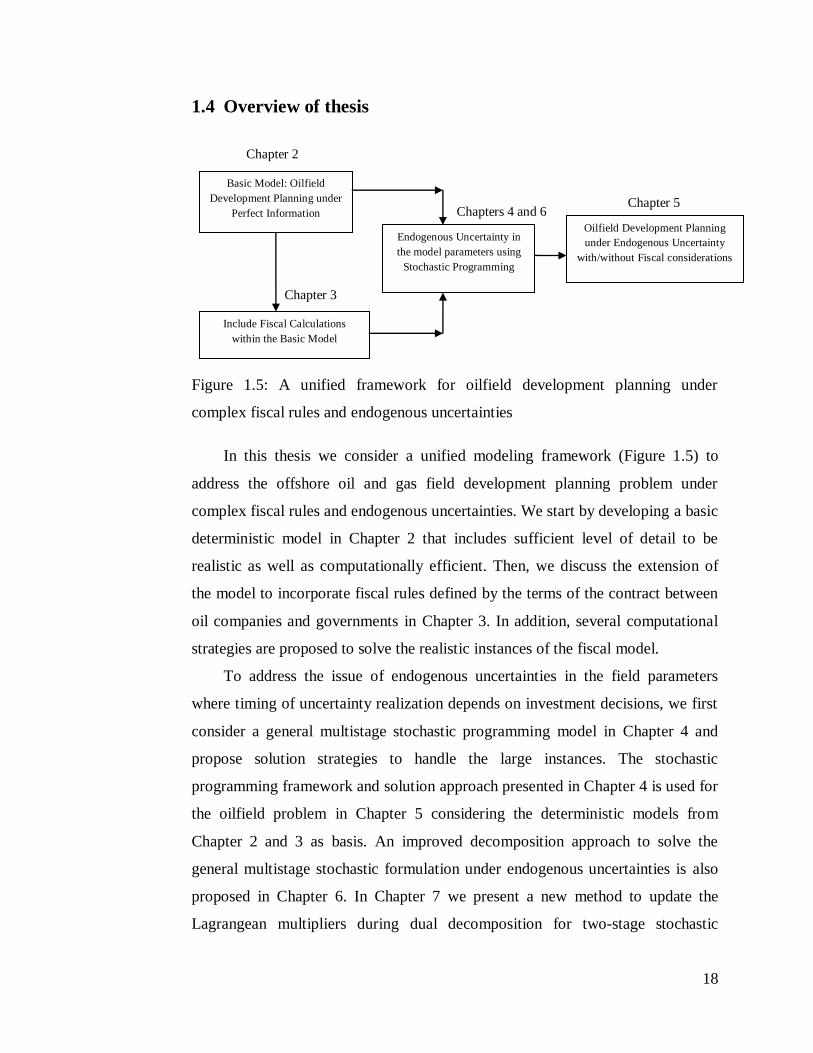
In this thesis we consider a unified modeling framework (Figure 1.5) to

address the offshore oil and gas field development planning problem under

complex fiscal rules and endogenous uncertainties. We start by developing a basic

deterministic model in Chapter 2 that includes sufficient level of detail to be

realistic as well as computationally efficient. Then, we discuss the extension of

the model to incorporate fiscal rules defined by the terms of the contract between

oil companies and governments in Chapter 3. In addition, several computational

strategies are proposed to solve the realistic instances of the fiscal model.

To address the issue of endogenous uncertainties in the field parameters

where timing of uncertainty realization depends on investment decisions, we first

consider a general multistage stochastic programming model in Chapter 4 and

propose solution strategies to handle the large instances. The stochastic

programming framework and solution approach presented in Chapter 4 is used for

the oilfield problem in Chapter 5 considering the deterministic models from

Chapter 2 and 3 as basis. An improved decomposition approach to solve the

general multistage stochastic formulation under endogenous uncertainties is also

proposed in Chapter 6. In Chapter 7 we present a new method to update the

Lagrangean multipliers during dual decomposition for two-stage stochastic

Chapter 5 Chapters 4 and 6

Chapter 3

Chapter 2

Basic Model: Oilfield

Development Planning under

Perfect Information

Include Fiscal Calculations

within the Basic Model

Endogenous Uncertainty in

the model parameters using

Stochastic Programming

Oilfield Development Planning

under Endogenous Uncertainty

with/without Fiscal considerations

19

mixed-integer linear programs under exogenous uncertainties. A more detailed

overview of the chapters in the thesis is presented below:

1.4.1 Chapter 2

Chapter 2 presents an efficient basic deterministic model for offshore oil and gas

field development problem. In particular, we develop a multiperiod non-convex

MINLP model for multi-field site that includes three components (oil, water and

gas) explicitly in the formulation using higher order polynomials avoiding bilinear

and other nonlinear terms. With the objective of maximizing total NPV for long-

term planning horizon, the model involves decisions related to FPSO (floating

production, storage and offloading) installation and expansions, field-FPSO

connections, well drilling and production rates in each time period. Furthermore,

it is reformulated into an MILP after piecewise linearization and exact

linearization techniques that can be solved to global optimality in an efficient

way. Solutions of realistic instances involving 10 fields, 3 FPSOs, 84 wells and 20

years planning horizon are reported, as well as comparisons between the

computational performance of the proposed MINLP and MILP formulations.

1.4.2 Chapter 3

In Chapter 3, we extend the simple NPV (net present value) based optimal oilfield

development planning model developed in Chapter 2 to include general complex

fiscal rules having progressive fiscal terms and ringfencing provisions. The

progressive fiscal terms penalize higher production rates based on the certain

profitability measures such as cumulative oil produced, daily production, rate of

return defined in the contract. On the other hand, ringfencing provisions divide

the fields in certain groups such that only fields in a given ringfence can share the

cost and revenues for fiscal calculations, but not with the fields from other

ringfences. Therefore, these provisions further increase the complexity of the

model. We explain the reduction of the proposed fiscal model to a variety of

contracts. The impact of the explicit consideration of the fiscal terms during

oilfield development planning on the investment and operating decisions is

analyzed. Since, the fiscal model can become computationally very expensive to

20

solve, we propose logic constraints and valid inequalities to reformulate the model

that can be solved more efficiently. A relaxation scheme and an approximation

technique are also provided that work as good heuristics for the large-scale

problems. The proposed model and computational strategies are applied to several

instances of the oilfield development problems with fiscal contracts. Preliminary

results on a bi-level decomposition approach are provided that can predict the

rigorous bounds for the large instances involving ringfencing provisions.

1.4.3 Chapter 4

Chapter 4 considers a general multistage stochastic mixed-integer linear

programming (MSSP) model with endogenous uncertainty in some of the

parameters, where the optimization decisions affect the times when the

uncertainties in those parameters are resolved. To address the issue that the

number of non-anticipativity (NA) constraints increases exponentially with the

number of uncertain parameters and/or its realizations, we present a new

theoretical property that significantly reduces the problem size and complements

two previous properties proposed by Goel and Grossmann (2006). Since one

might generate reduced models that are still too large to be solved directly, we

also propose three solution strategies: a k-stage constraint strategy where we only

include the NA constraints up to a specified number of stages, an iterative NAC

relaxation strategy, and a Lagrangean decomposition algorithm that decomposes

the problem into scenarios. Numerical results for two process network examples

are presented to illustrate the performance of the proposed solution strategies.

1.4.4 Chapter 5

Chapter 5 presents a multistage stochastic programming model for investment and

operations planning of offshore oil and gas field infrastructure. In particular, we

consider the deterministic models proposed in Chapters 2 and 3 as basis, and

utilize the stochastic programming framework presented in Chapter 4 to formulate

the model with/without fiscal contracts. We also consider correlations among the

endogenous uncertain parameters for a field such as field size, oil deliverability,

water-oil ratio and gas-oil ratio, which reduce the total number of scenarios in the

21

resulting multistage stochastic formulation. To solve the large instances of the

problem, the Lagrangean decomposition approach proposed in Chapter 4 allowing

parallel solution of the scenario subproblems is implemented in the GAMS grid

computing environment. Computational results on a variety of oilfield

development planning examples are presented to illustrate the efficiency of the

model and the decomposition approach.

1.4.5 Chapter 6

In Chapter 6, we propose a new decomposition algorithm for solving general

large-scale multistage stochastic programs (MSSP) with endogenous

uncertainties. Instead of dualizing all the initial non-anticipativity constraints

(NACs) and removing all the conditional non-anticipativity constraints to

decompose the problem into scenario subproblems as in Chapters 4 and 5, the

basic idea relies on a partial decomposition scheme. It is proved that the algorithm

provides a dual bound that is at least as tight as the standard approach. The

algorithm has been applied to process network examples and oilfield development

planning problem to compare the quality of the bounds obtained at the root node

and impact on the computational effort.

1.4.6 Chapter 7

Chapter 7 presents a method for improving the dual bound of decomposable

MILP models using integer programming sensitivity analysis based on the

previous work by Tarhan (2009). In particular, it proposes a new linear program

that involves constraints from the primal and dual sensitivity analysis (Dawande

and Hooker, 2000) using the information from branch and bound tree of each

subproblem solution during Lagrangean decomposition, and yields improved

multipliers which results in faster convergence of the algorithm. The method has

been applied to several example problems to compare its performance against

standard subgradient method.

22

1.4.7 Chapter 8

Chapter 8 provides a summary of the major contributions of the thesis and

suggestions for future work.

This thesis has led to the following papers:

Gupta, V., Grossmann, I. E., 2011a. Solution Strategies for Multistage

Stochastic Programming with Endogenous Uncertainties. Computers and

Chemical Engineering 35, 2235–2247.

Gupta, V., Grossmann, I. E., 2011b. Offshore Oilfield Development

Planning under Uncertainty and Fiscal Considerations. Optimization and

Analytics in the Oil and Gas Industry, Part I; Springer Edition, submitted

for publication.

Gupta, V., Grossmann, I. E., 2012a. An Efficient Multiperiod MINLP

Model for Optimal planning of Offshore Oil and Gas Field Infrastructure.

Industrial and Engineering Chemistry Research 51 (19), 6823–6840.

Gupta, V., Grossmann, I. E., 2012b. Modeling and Computational

Strategies for Offshore Oilfield Development Planning under Complex

Fiscal Rules. Industrial and Engineering Chemistry Research 51,

14438−14460.

Gupta, V., Grossmann, I. E., 2013a. Multistage Stochastic Programming

Approach for Offshore Oilfield Infrastructure Planning under Production

Sharing Agreements and Endogenous Uncertainties, manuscript in

preparation.

Gupta, V., Grossmann, I. E., 2013b. A new Decomposition Algorithm for

Multistage Stochastic Programs with Endogenous Uncertainties, submitted

for publication.

Tarhan, B., Gupta V., Grossmann, I. E., 2013. Improving Dual Bound for

Stochastic MILP Models using Sensitivity Analysis, to be submitted.

23

Chapter 2

An efficient multiperiod MINLP

model for optimal planning of

offshore oil and gas field

infrastructure

2.1 Introduction

In this chapter, we focus on developing a basic deterministic model for the

strategic/tactical planning of offshore oil and gas fields, which includes sufficient

level of details to be useful for realistic oilfield development projects, as well as it

can be extended to include fiscal and uncertainty considerations as in the

subsequent chapters. In particular, there are following major extensions and

differences that are addressed in the proposed deterministic model as compared to

the previous work:

(1) We consider three components (oil, water and gas) explicitly in the

formulation for a multi-field site, which allows considering realistic

problems for facility installation and capacity decisions.

(2) Nonlinear reservoir behavior in the model is approximated by 3rd

and

higher order polynomials to ensure sufficient accuracy for the predicted

reservoir profiles.

(3) The number of wells is used as a variable for each field to capture the

realistic drill rig limitations and the resulting trade-offs among various

fields.

24

(4) We include the possibility of expanding the facility capacities in the

future, and including the lead times for construction and expansions for

each facility to ensure realistic investments.

A typical offshore oilfield infrastructure (Figure 2.1) consists of various

production facilities such as Floating Production, Storage and Offloading (FPSO),

fields, wells and connecting pipelines to produce oil and gas from the reserves.

Each oilfield consists of a number of potential wells to be drilled using drilling

rigs, which are then connected to the facilities through pipelines to produce oil.

There is a multi-phase flow in these pipelines due to the presence of gas and

liquid that comprises oil and water. Therefore, there are three main components

present, and their relative amounts depend on certain parameters like cumulative

oil produced. The field to facility connection involves trade-offs associated to the

flowrates of oil and gas for a particular field-facility connection, connection costs,

and possibility of other fields to connect to that same facility, while the number of

wells that can be drilled in a field depends on the availability of the drilling rig

that can drill a certain number of wells each year.

We assume in this work that the type of offshore facilities connected to fields

to produce oil and gas are FPSOs with continuous capacities and ability to expand

them in the future. These FPSO facilities costs multi-billion dollars each

depending on their sizes and have the capability of operating in remote locations

FPSO FPSO

Field

Field Field

Field

Total Oil/Gas

Production

Figure 2.1: Typical Offshore Oilfield Infrastructure Representation

25

for very deep offshore oilfields (200m-2000m) where seabed pipelines are not

cost effective. FPSOs are large ships that can process the produced oil and store

until it is shipped to the onshore site or sales terminal. Processing includes the

separation of oil, water and gas into individual streams using separators located at

these facilities. Each FPSO facility has a lead time between the construction or

expansion decision, and the actual availability. The wells are subsea wells in each

field that are drilled using drilling ships. Therefore, there is no need to have a

facility present to drill a subsea well. The only requirement to recover oil from it

is that the well must be connected to a FPSO facility.

The facilities and connection involved in the offshore planning are often in

operation over many years, and it is therefore important to take future conditions

into consideration when designing an initial infrastructure or any expansions. This

can be incorporated by dividing the planning horizon, for example, 20 years, into

a number of time periods with a length of 1 year, and allowing investment and

operating decisions in each period, which leads to a multi-period planning

problem.

When oil is extracted from a reservoir oil deliverability, water-to-oil ratio

(WOR) and gas-to-oil ratio (GOR) change nonlinearly as a function of the

cumulative oil recovered from the reservoir. The initial oil and gas reserves in the

reservoirs, as well as the relationships for WOR and GOR in terms of fractional

oil recovery (fc), are estimated from geologic studies. Figures 2.2 (a)–(c) represent

the oil deliverability from a field per well, WOR and GOR versus fractional oil

recovered from that field. We can see from these figures that there are different

nonlinear field profiles for different field-FPSO connections to account for the

variations in the flows for each of these possible connections.

The maximum oil flowrate (field deliverability) per well can be represented

as a 3rd

order polynomial equation (2.1) in terms of the fractional oil recovery.

Furthermore, the actual oil flowrate (xf ) from each of the wells is restricted by

both the field deliverabilityd

fQ , eq. (2.2), and facility capacity. We assume that

there is no need for enhanced recovery, i.e., no need for injection of gas or water

into the reservoir. The oil produced from the wells (xf ) contains water and gas

26

and their relative rates depend on water-to-oil ratio (worf) and gas-to-oil ratio

(gorf) that are approximated using 3rd

order polynomial functions in terms of

fractional oil recovered (eqs. (2.3)-(2.4)). The water and gas flow rates can be

calculated by multiplying the oil flowrate (xf ) with water-to-oil ratio and gas-to-

oil ratio as in eqs. (2.5) and (2.6), respectively. Note that the reason for

considering fractional oil recovery compared to cumulative amount of oil was to

avoid numerical difficulties that could arise due to very small magnitude of the

polynomial coefficients in that case.

1,1

2

,1

3

,,1 )()( dfccfcbfcaQ fffftff

d

f

f (2.1)

d

ff Qx

f (2.2)

ffffffff dfccfcbfcawor ,2,2

2

,2

3

,2 )()(

f (2.3)

ffffffff dfccfcbfcagor ,3,3

2

,3

3

,3 )()(

f (2.4)

fff xworw

f (2.5)

fff xgorg

f (2.6)

In Appendix A we derive the polynomial equations for the cumulative water

and cumulative gas produced as a function of fractional oil recovery using

equations (2.3) and (2.4), respectively, in order to avoid the bilinear terms (2.5)-

(2.6) that are required in the model based on the above reservoir equations. Notice

that in this chapter we focus on a multi-field site and include sufficient details in

the model to account for the various trade-offs involved without going into much

detail for each of these fields. However, the proposed model can easily be

extended to include various facility types and other details in the oilfield

development planning problem.

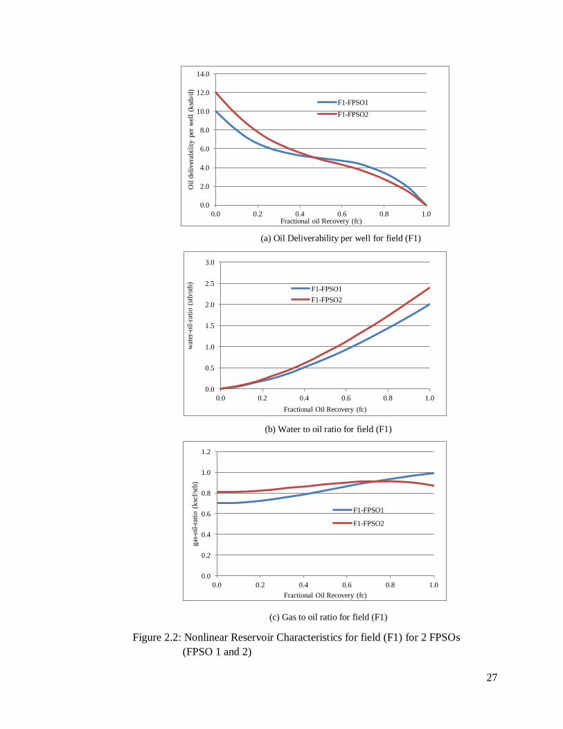
27

Figure 2.2: Nonlinear Reservoir Characteristics for field (F1) for 2 FPSOs

(FPSO 1 and 2)

0.0

2.0

4.0

6.0

8.0

10.0

12.0

14.0

0.0 0.2 0.4 0.6 0.8 1.0

Oil

del

iver

abil

ity p

er w

ell

(kst

b/d

)

Fractional oil Recovery (fc)

F1-FPSO1

F1-FPSO2

0.0

0.5

1.0

1.5

2.0

2.5

3.0

0.0 0.2 0.4 0.6 0.8 1.0

wat

er-o

il-r

atio

(st

b/s

tb)

Fractional Oil Recovery (fc)

F1-FPSO1

F1-FPSO2

0.0

0.2

0.4

0.6

0.8

1.0

1.2

0.0 0.2 0.4 0.6 0.8 1.0

gas

-oil

-rat

io (

ksc

f/st

b)


F1-FPSO1

F1-FPSO2

(a) Oil Deliverability per well for field (F1)

(b) Water to oil ratio for field (F1)

(c) Gas to oil ratio for field (F1)

28

The outline of this chapter is as follows. In section 2.2, we provide a formal

description of the oilfield development problem considered that is formulated as

an MINLP problem in section 2.3. The MINLP model is then reformulated as an

MILP problem in section 2.4. Furthermore, section 2.5 introduces a procedure to

reformulate both the models with reduced number of binary variables. Section 2.6

presents numerical results on the three realistic oilfield development cases

involving up to 10 oilfields, 20 years of planning horizon and 84 wells, and

compares the performance of the proposed models.

2.2 Problem Statement

Given is a typical offshore oilfield infrastructure consisting of a set of oil fields F

= {1,2,…} available for producing oil using a set of FPSO (Floating, Production,

Storage and Offloading) facilities, FPSO = {1,2,…}, (see Figure 2.1). To produce

oil from a field, it must be connected to a FPSO facility that can process the

produced oil, store and offload it to the other tankers.

We assume that the location of each FPSO facility and its possible

connections to the given fields are known (Figure 2.1). Notice that each FPSO

facility can be connected to more than one field to produce oil while a field can

only be connected to a single FPSO facility. In addition, the potential number of

wells in each field is also given. There can be a significant amount of water and

gas that comes out with the oil during the production process that needs to be

considered while planning for FPSO capacity installations and expansions. The

water is usually re-injected after separation from the oil while the gas can be sold

in the market. In this case for simplicity we do not consider water or gas re-

injection i.e. natural depletion of the reserves.

To develop and operate such a complex and capital intensive offshore

oilfield infrastructure, we have to make the optimum investment and operation

decisions to maximize the net present value considering a long-term planning

horizon. The planning horizon is discretized into a number of time periods t,

typically each with 1 year of duration. Investment decisions in each time period t

include which FPSO facilities should be installed or expanded, and their

29

respective installation or expansion capacities for oil, liquid and gas, which fields

should be connected to which FPSO facility, and the number of wells that should

be drilled in a particular field f given the restrictions on the total number of wells

that can be drilled in each time period t over all the given fields. Operating

decisions include the oil/gas production rates from each field f in each time period

t. It is assumed that all the installation and expansion decisions occur at the

beginning of each time period t, while operation takes place throughout the time

period. There is a lead time of l1 years for each FPSO facility initial installation

and a lead time of l2 years for the expansion of an earlier installed FPSO facility.

Once installed, we assume that the oil, liquid (oil and water) and gas capacities of

a FPSO facility can be expanded only once.

Field deliverability, i.e. maximum oil flowrate from a field, WOR and GOR

are approximated by a cubic equations, while cumulative water produced and

cumulative gas produced from a field are represented by fourth order polynomials

in terms of the fractional oil recovered from that field. Notice that these 4th

order

polynomials correspond to the integration of the cubic equations for WOR and

GOR as explained in Appendix A. The motivation for using polynomials for

cumulative water produced and cumulative gas produced as compared to WOR

and GOR is to avoid bilinear terms in the formulation and to allow converting the

resulting model into an MILP formulation. Furthermore, all the wells in a

particular field f are assumed to be identical for the sake of simplicity leading to

the same reservoir profiles, eqs. (2.1)-(2.6), for each of these wells. However, the

model can easily be extended to include different reservoir profiles for each of

these wells for a specific field-FPSO connection, which may result in a significant

increase in the computational effort due to the additional nonlinearities and

constraints in the model.

2.3 MINLP Model

We present in this section a multiperiod MINLP model for the offshore oil and

gas field infrastructure optimization problem. Reader should refer to the

nomenclature section at the end of this chapter for the definitions of the various

30

parameters and variables used in the model. The objective function (2.7) is to

maximize the total net present value (NPV) of the project. Constraint (2.8)

represents the overall NPV as a function of the difference between total revenue

and total cost in each time period t taking the discount factors dt into account.

NPVMax (2.7)

)( tt

t

t COSTREVdNPV

(2.8)

The total revenues (2.9) in each time period t are computed based on the total

amount of oil and gas produced in that time period and respective selling prices

where total oil, water and gas flowrates in each time period t, (tot

t

tot

t

tot

t gwx ,, )

are calculated as the sum of the production rate of these components over all the

FPSO facilities in equations (2.10)-(2.12), respectively.

)( tot

tt

tot

ttt gxREVt

t (2.9)

fpso

tfpso

tot

t xx ,

t (2.10)

fpso

tfpso

tot

t ww ,

t (2.11)

fpso

tfpso

tot

t gg ,

t (2.12)

The total cost incurred in (2.13) is the sum of capital and operating expenses

in each time period t. The overall capital expenses (2.14) consist of the fixed

installation costs for FPSO facilities, variable installation and expansion costs

corresponding to the FPSOs liquid and gas capacities, connection costs between a

field and a FPSO facility and cost of drilling the wells for each field in each time

period t. The total operating expenses (2.15) are the operation cost occurred

corresponding to the total amount of liquid and gas produced in each time period

t.

ttt OPERCAPCOST

t (2.13)

31

f fpso f

well

tf

well

tf

c

tfpsof

C

tfpsof

fpso

gas

tfpso

gas

tfpso

gas

tfpso

liq

tfpso

liq

tfpso

liq

tfpsotfpsotfpsot

IFCbFC

QEQIVCQEQIVCbFCCAP

,,,,,,

,,,,,,,, )()(

t (2.14)

tot

t

gas

t

tot

t

tot

t

liq

ttt gOCwxOCOPER )(

t (2.15)

Constraints (2.16)-(2.19) predict the reservoir behavior for each field f in

each time period t. In particular, constraint (2.16) restricts the oil flow rate from

each well for a particular FPSO-field connection in time period t to be less than

the deliverability (maximum oil flow rate) of that field per well where equation

(2.17) represents the field deliverability per well at the beginning of time period

t+1 for a particular FPSO-field connection as the cubic equation in terms of the

fractional oil recovered by the end of time period t from that field. Constraint

(2.17a) corresponds to the oil deliverability in time period 1 while (2.17b)

represents for the rest of time periods in the planning horizon. Constraints (2.18)

and (2.19) represent the value of water-to-oil and gas-to-oil ratios in time period t

for a specific field-FPSO connection as cubic equations in terms of the fractional

oil recovery by the end of previous time period, respectively.

welld

tfpsof

well

tfpsof Qx ,

,,,,

tfpsof ,, (2.16)

fpsof

welld

fpsof dQ ,,1

,

1,,

fpsof , (2.17a)

fpsoftffpsoftffpsoftffpsof

welld

tfpsof dfccfcbfcaQ ,,1,,,1

2

,,,1

3

,,,1

,

1,, )()(

Ttfpsof ,,

(2.17b)

fpsoftffpsoftffpsoftffpsoftfpsof dfccfcbfcawor ,,21,,,2

2

1,,,2

3

1,,,2,, )()(

tfpsof ,,

(2.18)

32

fpsoftffpsoftffpsoftffpsoftfpsof dfccfcbfcagor ,,31,,,3

2

1,,,3

3

1,,,3,, )()(

tfpsof ,,

(2.19)

The predicted WOR and GOR values in equations (2.18) and (2.19) are

further used in equations (2.20) and (2.21) to calculate the respective water and

gas flowrates from field to FPSO in time period t by multiplying it with the

corresponding oil flow rate. Notice that these equations give rise to the bilinear

terms in the model.

tfpsoftfpsoftfpsof xworw ,,,,,, tfpsof ,, (2.20)

tfpsoftfpsoftfpsof xgorg ,,,,,, tfpsof ,, (2.21)

The total oil flow rate in (2.22) from each field f in time period t is the sum

of the oil flow rates that are directed to FPSO facilities in that time period t,

whereas oil that is directed to a particular FPSO facility from a field f is calculated

as the multiplication of the oil flow rate per well and number of wells available

for production in that field, eq. (2.23).

fpso

tfpsoftf xx ,,,

tf , (2.22)

well

tfpsof

well

tftfpsof xNx ,,,,,

tfpsof ,, (2.23)

Eq. (2.24) computes the cumulative amount of oil produced from field f by

the end of time period t, while (2.25) represents the fractional oil recovery by the

end of time period t. The cumulative oil produced is also restricted in (2.26) by

the recoverable amount of oil from the field.

)(1

,,

t

ftf xxc

tf , (2.24)

f

tf

tfREC

xcfc

,

,

tf , (2.25)

ftf RECxc , tf ,

(2.26)

33

Eqs. (2.27)-(2.29) compute total oil, water and gas flow rates into each FPSO

facility, respectively, in time period t from all the given fields.

f

tfpsoftfpso xx ,,,

tfpso, (2.27)

f

tfpsoftfpso ww ,,,

tfpso, (2.28)

f

tfpsoftfpso gg ,,,

tfpso, (2.29)

There are three types of capacities i.e. oil, liquid (oil and water) and gas that

are used for modeling the capacity constraints for FPSO facilities. Specifically,

constraints (2.30)-(2.32) restrict the total oil, liquid and gas flow rates into each

FPSO facility to be less than its corresponding capacity in each time period t

respectively. These three different kinds of capacities of a FPSO facility in time

period t are computed by equalities (2.33)-(2.35) as the sum of the corresponding

capacity at the end of previous time period t-1, installation capacity at the

beginning of time period t-l1 and expansion capacity at the beginning of time

period t-l2. Specifically, the termoil

ltfpsoQI1, in equation (2.33) represents the oil

capacity of a FPSO facility that started to install l1 years earlier and is expected to

be ready for production in time period t, to account for the lead time of l1 years for

a FPSO facility installation. The term oil

ltfpsoQE1, represents the expansion

decision in the oil capacity of an already installed FPSO facility that is taken l2

years before time period t, to consider the lead time of l2 years for capacity

expansion. Similarly, the corresponding terms in equations (2.34) and (2.35)

represent the lead times for liquid and gas capacity installation or expansion,

respectively. Notice that due to one installation and expansion of a FPSO facility,

oil

ltfpsoQI1, and

oil

ltfpsoQE1, can have non-zero values only once in the planning

horizon while oil

tfpsoQ 1, can be non-zero in the multiple time periods.

34

oil

tfpsotfpso Qx ,, tfpso,

(2.30)

liq

tfpsotfpsotfpso Qwx ,,,

tfpso, (2.31)

gas

tfpsotfpso Qg ,,

tfpso, (2.32)

oil

ltfpso

oil

ltfpso

oil

tfpso

oil

tfpso QEQIQQ21 ,,1,,

tfpso,

(2.33)

liq

ltfpso

liq

ltfpso

liq

tfpso

liq

tfpso QEQIQQ21 ,,1,,

tfpso,

(2.34)

gas

ltfpso

gas

ltfpso

gas

tfpso

gas

tfpso QEQIQQ21 ,,1,, tfpso, (2.35)

Inequalities (2.36) and (2.37) restrict the installation and expansion of a

FPSO facility to take place only once, respectively, while inequality (2.38) states

that the connection between a FPSO facility and a field can be installed only once

during the whole planning horizon. Inequality (2.39) ensures that a field can be

connected to at most one FPSO facility in each time period t, while (2.40) states

that at most one FPSO-field connection is possible for a field f during the entire

planning horizon T due to engineering considerations. Constraints (2.41) and

(2.42) state that the expansion in the capacity of a FPSO facility and the

connection between a field and a FPSO facility, respectively, in time period t can

occur only if that FPSO facility has already been installed by that time period.

1, Tt

tfpsob

fpso (2.36)

1, Tt

ex

tfpsob

fpso (2.37)

1,, Tt

c

tfpsofb

fpsof , (2.38)

1,, fpso

c

tfpsofb

tf , (2.39)

Tt fpso

c

tfpsofb 1,,

f

(2.40)

35

t

fpso

ex

tfpso bb1

,,

tfpso, (2.41)

t

fpso

c

tfpsof bb1

,,,

tfpsof ,, (2.42)

Inequality (2.43) states that the oil flow rate per well from a field f to a FPSO

facility in time period t will be zero if that FPSO-field connection is not available

in that time period. Notice that equations (2.23) and (2.43) ensure that for

production from a field in time period t there must be a field-FPSO connection

and at-least one well available in that field at the beginning of time period t.

Constraints (2.44)-(2.49) are the upper-bounding constraints on the installation

and expansion capacities for FPSO facilities in time period t corresponding to the

three different kinds of capacities mentioned earlier.

t

c

fpsof

oilwell

fpsof

well

tfpsof bUx1

,,

,

,,,

tfpsof ,, (2.43)

tfpso

oil

fpso

oil

tfpso bUQI ,, tfpso,

(2.44)

tfpso

liq

fpso

liq


(2.45)

tfpso

gas

fpso

gas


(2.46)

ex

tfpso

oil

fpso

oil

tfpso bUQE ,, tfpso,

(2.47)

ex

tfpso

liq

fpso

liq

tfpso bUQE ,, tfpso,

(2.48)

exp

,, tfpso

gas

fpso

gas

tfpso bUQE

tfpso, (2.49)

The additional restrictions on the oil, liquid and gas expansion capacities of

FPSO facilities, (2.50)-(2.52), come from the fact that these expansion capacities

should be less than a certain fraction (µ) of the initial built capacities,

respectively. Notice that available capacities in the previous time period can be

used in the expression instead of initially built FPSO capacities given that only

one installation and expansion is allowed for each of these facilities.

oil

tfpso

oil

tfpso QQE 1,,

tfpso, (2.50)

36

liq

tfpso

liq

tfpso QQE 1,,

tfpso, (2.51)

gas

tfpso

gas

tfpso QQE 1,,

tfpso, (2.52)

The number of wells available for the production from a field is calculated

from (2.53) as the sum of the wells available at the end of previous time period

and the number of wells drilled at the beginning of time period t. The maximum

number of wells that can be drilled over all the fields during each time period t

and in each field f during complete planning horizon T are restricted by respective

upper bounds in (2.54) and (2.55). Notice that the important resource restriction

due to the availability of drill rigs as in constraint (2.54) makes the proposed

model more practical and useful. This restriction can easily be removed by

relaxing this constraint if there are no drilling limitations. Moreover, the resulting

model, which can be considered as a specific case of the proposed model, will

most likely become easier to solve.

wellwell

tf

well

tf tfINN

,1,,

tf , (2.53)

well

t

f

well

tf UII ,

t

(2.54)

well

f

well

tf UNN , tf ,

(2.55)

The non-convex MINLP model (Model 1) for offshore oilfield investment

and operations planning involves constraint (2.7)-(2.55). In particular, constraints

(2.17b)- (2.21) and (2.23) are nonlinear and non-convex constraints in the model

that can lead to suboptimal solutions when solved with a method that assumes

convexity.

In contrast to Model 1, the proposed MINLP model (Model 2) involves all

the constraints as in Model 1 except (2.18)-(2.21) that are replaced with the

reservoir profiles based on cumulative water and cumulative gas produced for

each field-FPSO connection. The motivation for using polynomials for

cumulative water produced and cumulative gas produced as compared to WOR

and GOR is to avoid bilinear terms (2.20)-(2.21) in the formulation and allow

37

converting the resulting MINLP model into an MILP formulation. In particular,

the cumulative water and cumulative gas produced by the end of time period t

from a field are represented by 4th

order polynomial equations (2.56) and (2.57),

respectively, in terms of fractional oil recovery by the end of time period t. Notice

that these 4th

order polynomials (2.56) and (2.57) correspond to the cubic

equations for WOR and GOR, respectively, that are derived in Appendix A.

tffpsoftffpsoftffpsoftffpsof

wc

tfpsof fcdfccfcbfcaQ ,,,2

2

,,,2

3

,,,2

4

,,,2,, )()()(

tfpsof ,,

(2.56)

tffpsoftffpsoftffpsoftffpsof

gc

tfpsof fcdfccfcbfcaQ ,,,3

2

,,,3

3

,,,3

4

,,,3,, )()()(

tfpsof ,,

(2.57)

Notice that variables wc

tfpsofQ ,, and

gc

tfpsofQ ,, will be non-zero in equations

(2.56) and (2.57) if tffc , is non-zero even though that particular field-FPSO

connection is not present. Therefore, wc

tfpsofQ ,, and gc

tfpsofQ ,, represent dummy

variables in equations (2.56) and (2.57) instead of actual cumulative water (

tfpsofwc ,, ) and cumulative gas ( tfpsofgc ,, ) recoveries due to the fact that only

those cumulative water and cumulative gas produced can be non-zero that has the

specific FPSO-field connection present in that time period t. Therefore, we

introduce constraints (2.58)-(2.61) to equate the actual cumulative water

produced, tfpsofwc ,, , for a field-FPSO connection by the end of time period t to

the corresponding dummy variable wc

tfpsofQ ,, only if that field-FPSO connection is

present in time period t else tfpsofwc ,, is set to zero. Similarly, constraints (2.62)-

(2.65) equate the actual cumulative gas produced, tfpsofgc ,, , to the dummy

variable gc

tfpsofQ ,, only if that field-FPSO connection is present in time period t,

otherwise it is set to zero.

wc

fpsofM , and gc

fpsofM , correspond to maximum amount

of cumulative water and gas that can be produced for a particular field and FPSO

38

connection during the entire planning horizon, respectively. Note that the

motivation for using dummy variables (wc

tfpsofQ ,, andgc

tfpsofQ ,, ) for cumulative

water and cumulative gas flows in equations (2.56)-(2.57) followed by big-M

constraints (2.58)-(2.65), instead of using disaggregated variables for the

fractional recovery in equations (2.56)-(2.57) directly, was to avoid large number

of SOS1 variables while MILP reformulation of this model as explained in the

next section.

t

c

fpsof

wc

fpsof

wc

tfpsoftfpsof bMQwc1

,,,,,,, )1(

tfpsof ,, (2.58)

t

c

fpsof

wc

fpsof

wc

tfpsoftfpsof bMQwc1

,,,,,,, )1(

tfpsof ,, (2.59)

t

c

fpsof

wc

fpsoftfpsof bMwc1

,,,,,

tfpsof ,, (2.60)

t

c

fpsof

wc

fpsoftfpsof bMwc1

,,,,,

tfpsof ,, (2.61)

t

c

fpsof

gc

fpsof

gc

tfpsoftfpsof bMQgc1

,,,,,,, )1(

tfpsof ,, (2.62)

t

c

fpsof

gc

fpsof

gc

tfpsoftfpsof bMQgc1

,,,,,,, )1(

tfpsof ,, (2.63)

t

c

fpsof

gc

fpsoftfpsof bMgc1

,,,,,

tfpsof ,, (2.64)

t

c

fpsof

gc

fpsoftfpsof bMgc1

,,,,,

tfpsof ,, (2.65)

Eq. (2.66) and (2.67) compute the water and gas flow rates in time period t

from a field to FPSO facility as the difference of cumulative amounts produced by

the end of current time period t and previous time period t-1 divided by the time

duration of that period.

ttfpsoftfpsoftfpsof wcwcw /)( 1,,,,,,

tfpsof ,, (2.66)

ttfpsoftfpsoftfpsof gcgcg /)( 1,,,,,,

tfpsof ,, (2.67)

39

The non-convex MINLP model (Model 2) involves constraint (2.7)-(2.17)

and (2.22)-(2.67) where constraints (2.17b), (2.56) and (2.57) are univariate

polynomials while constraint (2.23) involves bilinear terms with integer variables.

The correspondence between reservoir profiles for both the MINLP models and

their comparison is presented in Appendices A and B, respectively. In the

following section, we reformulate MINLP Model 2 into an MILP problem that

can be solved to global optimality in an effective way. Notice that due to the

presence of bilinear terms in equations (2.20) and (2.21), Model 1 cannot be

reformulated into an MILP problem.

2.4 MILP Reformulation

The nonlinearities involved in Model 2 include univariate polynomials (2.17b),

(2.56), (2.57) and bilinear equations (2.23). In this section, we reformulate this

model into an MILP model, Model 3 using piecewise linearization and exact

linearization techniques that can give the global solution of the resulting

approximate problem.

To approximate the 3rd

and 4th order univariate polynomials (2.17b), (2.56)

and (2.57) SOS1 variablesl

tfb , are introduced to select the adjacent points l-1 and

l for interpolation over an interval l. Constraints (2.68)-(2.71) represent the

piecewise linear approximation for the fractional recovery and corresponding oil

deliverability, cumulative water and cumulative gas produced for a field in each

time period t, respectively, wherelcf

~,

lwelld

fpsofQ ,,

,

~,

lwc

fpsofQ ,

,

~and

lgc

fpsofQ ,

,

~are the

values of the corresponding variables at point l used in linear interpolation based

on the reservoir profiles (2.17b), (2.56) and (2.57). Note that only l

tfb , variables

are sufficient to approximate the constraints (2.17b), (2.56) and (2.57) by

selecting a specific value of the fractional recovery for each field in each time

period t that applies to all possible field-FPSO connections for that field. This

avoids the requirement of a large number of SOS1 variables and resulting increase

in the solution times that would have been required in the case if constraints

40

(2.56) and (2.57) were represented in terms of the disaggregated variables for

fractional recovery in Model 2.

n

l

ll

tftf cffc1

,,

~

tf ,

(2.68)

n

l

lwelld

fpsof

l

tf

welld

tfpsof QQ1

,,

,,

,

1,,

~

Ttfpsof ,,

(2.69)

n

l

lwc

fpsof

l

tf

wc

tfpsof QQ1

,

,,,,

~

tfpsof ,,

(2.70)

n

l

lgc

fpsof

l

tf

gc

tfpsof QQ1

,

,,,,

~

tfpsof ,,

(2.71)

Equation (2.72) allows only one of the point l to be selected for which l

tfb ,

equals 1 while equation (2.73) states that l

tf , can be non-zero for only two

consecutive points l and l-1 that are used for convex combination during

interpolation, eq. (2.74). Thus, the corresponding lth piece is used for linear

interpolation as all other l

tf , are zero for a field in time period t and determines

the value of the interpolated variable as a convex combination of their values at

both the end of this piece l in equations (2.68)-(2.71).

1

1

, 1n

l

l

tfb

tf , (2.72)

l

tf

l

tf

l

tf bb ,

1

,,

ltf ,, (2.73)

n

l

l

tf

1

, 1

tf , (2.74)

The other nonlinear constraints (2.23) in Model 2 contain bilinear terms that

can be linearized using exact linearization (Glover, 1975). To linearize constraint

(2.23) we first express the integer variable,well

tfN , , for the number of wells in

terms of the binary variableswell

tkfZ ,, using eq. (2.75) where

well

tkfZ ,, determines the

value of the kth term of the binary expansion.

41

k

well

tkf

kwell

tf ZN ,,

1

, 2

tf ,

(2.75)

The bilinear term in constraint (2.23) can then be rewritten as follows,

k

well

tfpsof

well

tkf

k

tfpsof xZx ,,,,

1

,, 2

tfpsof ,, (2.76)

Constraint (2.76) can be reformulated as a linear constraint (2.77) by

introducing a nonnegative continuous variablewell

tfpsof

well

tkf

well

tkfpsof xZZX ,,,,,,,

which is further defined by constraints (2.78)-(2.81) by introducing an auxiliary

variablewell

tkfpsofZX ,,,1 .

k

well

tkfpsof

k

tfpsof ZXx ,,,

1

,, 2

tfpsof ,, (2.77)

well

tfpsof

well

tkfpsof

well

tkfpsof xZXZX ,,,,,,,, 1

tkfpsof ,,, (2.78)

well

tkf

well

fpsof

well

tkfpsof ZUZX ,,,,,,

tkfpsof ,,, (2.79)

)1(1 ,,,,,,

well

tkf

well

fpsof

well

tkfpsof ZUZX

tkfpsof ,,, (2.80)

01,0 ,,,,,, well

tkfpsof

well

tkfpsof ZXZX

tkfpsof ,,, (2.81)

The reformulated MILP Model 3 involves constraints (2.7)-(2.16), (2.17a),

(2.22), (2.24)-(2.55), (2.58)-(2.75) and (2.77)-(2.81) which are linear and mixed-

integer linear constraints and allow to solve this approximate problem to global

optimality using standard mixed-integer linear programming solvers.

Remarks

The previous two sections present a multiperiod MINLP model for the

oilfield investment and operations planning problem for long-term planning

horizon and its reformulation as an MILP model using linearization techniques.

The MINLP models involve non-convexities and can yield suboptimal solutions

when using an MINLP solver that relies on convexity assumptions, while the

reformulated MILP model is guaranteed to be solved to global optimality using

linear programming based branch and cut methods. However, given the

difficulties involved in solving large scale instances of the MINLP and MILP

42

models, especially due to the large number of binary variables, we extend these

formulations by reducing the number of the binary variables. The next section

describes the proposed procedure for binary reduction for MINLP and MILP

formulations.

2.5 Reduced MINLP and MILP models

Due to the potential computational expense of solving the large scale MINLP and

MILP models presented in the previous sections, we further reformulate them by

removing many binary variables, namelyC

tfpsofb ,, . These binary variables

represent the timing of the connections between fields and FPSOs and are used

for discounting the connection cost in the objective function along with some

logic constraints in the proposed models. The motivation for binary reduction

comes from the fact that in the solution of these models the connection cost is

only ~2-3% of the total cost, and hence, this cost can be removed from the

objective function as its exact discounting does not have a significant impact on

the optimal solution. In particular, we propose to drop the index t fromC

tfpsofb ,, ,

which results in a significant decrease in the number of binary variables (~33%

reduction) and the solution time can be improved significantly for both the

MINLP and MILP formulations.

Therefore, to formulate the reduced models that correspond to Model 2 and 3

we use the binary variables R

fpsofb , to represent the connection between field and

FPSOs instead of using C

tfpsofb ,, which results in a significant decrease in the

number of binary variables in the model. As an example, for a field with 5

possible FPSO connections and 20 years planning horizon, the number of binary

variables required can be reduced from 100 to 5. The connection cost term in the

eq. (2.14) is also removed as explained above yielding constraint (2.82).

Moreover, some of the constraints in the previous MINLP and MILP models that

involve binary variablesC

tfpsofb ,, are reformulated to be valid for R

fpsofb , based

reduced model, i.e. constraints (2.83)-(2.93). Notice that constraints (2.93) and

43

(2.23) ensure that the oil flow rate from a field to FPSO facility in time period t,

tfpsofx ,, , will be non-zero only if that particular field-FPSO connection is installed

and there is at-least one well available in that field for production in time period t,

i.e. R

fpsofb , equals 1 andwell

tfN , is non-zero, otherwise tfpsofx ,, is set to zero.

Moreover, it may be possible that variable well

tfpsofx ,, can take non-zero value in

equation (2.93) if R

fpsofb , equals 1 even though there is no well available in that

field in time period t, but this will not have any effect on the solution given that

the fractional recovery from a field and other calculations/constraints in the model

are based on the actual amount of oil produced from the field, i.e. variable tfpsofx ,,

which is still zero in this case. Therefore, variable well

tfpsofx ,, can be considered as a

dummy variable in the reduced model.

f

well

tf

well

tf

fpso

gas

tfpso

gas

tfpso

gas

tfpso

liq

tfpso

liq

tfpso

liq

tfpsotfpsotfpsot

IFC

QEQIVCQEQIVCbFCCAP

,,

,,,,,,,, )()(

t (2.82)

)1( ,,,,,,

R

fpsof

wc

fpsof

wc

tfpsoftfpsof bMQwc

tfpsof ,, (2.83)

)1( ,,,,,,

R

fpsof

wc

fpsof

wc

tfpsoftfpsof bMQwc

tfpsof ,, (2.84)

R

fpsof

wc

fpsoftfpsof bMwc ,,,,

tfpsof ,, (2.85)

R

fpsof

wc

fpsoftfpsof bMwc ,,,,

tfpsof ,, (2.86)

)1( ,,,,,,

R

fpsof

gc

fpsof

gc

tfpsoftfpsof bMQgc

tfpsof ,, (2.87)

)1( ,,,,,,

R

fpsof

gc

fpsof

gc

tfpsoftfpsof bMQgc

tfpsof ,, (2.88)

R

fpsof

gc

fpsoftfpsof bMgc ,,,,

tfpsof ,, (2.89)

44

R

fpsof

gc

fpsoftfpsof bMgc ,,,,

tfpsof ,, (2.90)

1, fpso

R

fpsofb

f (2.91)

t

fpso

R

fpsof bb1

,,

tfpsof ,, (2.92)

R

fpsof

oilwell

fpsof

well

tfpsof bUx ,

,

,,,

tfpsof ,, (2.93)

The non-convex MINLP Model 2R for offshore oilfield investment and

operations planning after binary reduction involves constraints (2.7)-(2.13),

(2.15)-(2.17), (2.22)-(2.37), (2.41), (2.44)-(2.57), (2.66)-(2.67) and (2.82)-(2.93).

The reformulated MILP Model 3R after binary reduction involves constraints

(2.7)-(2.13), (2.15)-(2.16), (2.17a), (2.22), (2.24)-(2.37), (2.41), (2.44)-(2.55),

(2.66)-(2.75) and (2.77)-(2.93) which are linear and mixed-integer linear

constraints. Similarly, Model 1R corresponds to the non-convex MINLP model,

which is based on WOR and GOR expressions after binary reduction as described

above.

The resulting reduced models with fewer binaries can be solved much more

efficiently as compared to the original models. To calculate the discounted cost of

connections between field and FPSOs that corresponds to the reduced model

solution, we use the well installation schedule well

tfN , from the optimal solution of

reduced models to find the Field-FPSO connection timing and subtract the

corresponding discounted connection cost from the optimal NPV of the reduced

model. The resulting NPV represents the optimal NPV of the original models in

case connection costs are relatively small.

2.6 Numerical Results

In this section we present 3 instances of the oilfield planning problem where we

consider from 3 to 10 fields while the time horizon ranges from 10 to 20 years.

The maximum number of possible FPSOs is taken 3 in all the instances. We

compare the computational results of the various MINLP and MILP models

proposed in the previous sections for these 3 instances. Table 2.1 summarizes the

45

main features of these MINLP and reformulated MILP models. In particular, the

reservoir profiles and respective nonlinearities involved in the models are

compared in the table.

Table 2.1: Comparison of the nonlinearities involved in 3 model types

Model 1 Model 2 Model 3

Model Type MINLP MINLP MILP

Oil Deliverability 3rd order polynomial 3rd order polynomial Piecewise Linear

WOR 3rd order polynomial - -

GOR 3rd order polynomial - -

wc - 4th order polynomial Piecewise Linear

gc - 4th order polynomial Piecewise Linear

Bilinear Terms N*x

x*WOR

x*GOR

N*x None

MILP Reformulation Not Possible Possible Reformulated MILP

2.6.1 Instance 1

In this instance (Figure 2.3) we consider 3 oil fields that can be connected to

3 FPSOs with 7 possible connections among these fields and FPSOs. There are a

total of 25 wells that can be drilled, and the planning horizon considered is 10

years, which is discretized into 10 periods of each 1 year of duration. We need to

determine which of the FPSO facilities is to be installed or expanded, in what

time period, and what should be its capacity of oil, liquid and gas, to which fields

it should be connected and at what time, and the number of wells to be drilled in

FPSO 1 FPSO 3

Field 1

Field 3

Field 2

Figure 2.3: Instance 1 (3 Fields, 3 FPSOs, 10 years)

Total Oil/Gas

Production

FPSO 2

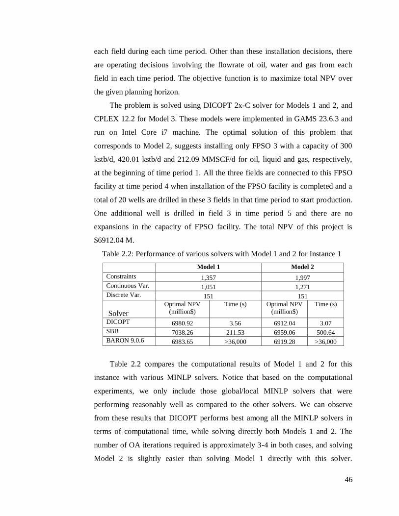
46

each field during each time period. Other than these installation decisions, there

are operating decisions involving the flowrate of oil, water and gas from each

field in each time period. The objective function is to maximize total NPV over

the given planning horizon.

The problem is solved using DICOPT 2x-C solver for Models 1 and 2, and

CPLEX 12.2 for Model 3. These models were implemented in GAMS 23.6.3 and

run on Intel Core i7 machine. The optimal solution of this problem that

corresponds to Model 2, suggests installing only FPSO 3 with a capacity of 300

kstb/d, 420.01 kstb/d and 212.09 MMSCF/d for oil, liquid and gas, respectively,

at the beginning of time period 1. All the three fields are connected to this FPSO

facility at time period 4 when installation of the FPSO facility is completed and a

total of 20 wells are drilled in these 3 fields in that time period to start production.

One additional well is drilled in field 3 in time period 5 and there are no

expansions in the capacity of FPSO facility. The total NPV of this project is

$6912.04 M.

Table 2.2: Performance of various solvers with Model 1 and 2 for Instance 1

Model 1 Model 2

Constraints 1,357 1,997

Continuous Var. 1,051 1,271

Discrete Var. 151 151

Solver

Optimal NPV

(million$)

Time (s) Optimal NPV

(million$)

Time (s)

DICOPT 6980.92 3.56 6912.04 3.07

SBB 7038.26 211.53 6959.06 500.64

BARON 9.0.6 6983.65 >36,000 6919.28 >36,000

Table 2.2 compares the computational results of Model 1 and 2 for this

instance with various MINLP solvers. Notice that based on the computational

experiments, we only include those global/local MINLP solvers that were

performing reasonably well as compared to the other solvers. We can observe

from these results that DICOPT performs best among all the MINLP solvers in

terms of computational time, while solving directly both Models 1 and 2. The

number of OA iterations required is approximately 3-4 in both cases, and solving

Model 2 is slightly easier than solving Model 1 directly with this solver.

47

However, the solutions obtained are not guaranteed to be the global solution. SBB

is also reasonable in terms of solution quality but it takes much longer time to

solve. BARON 9.0.6 can in principle find the global optimum solution to models

1 and 2, but it is very slow and takes more than 36,000s to be within ~23% and

~10% of optimality gap for these models, respectively. Note that we use the

DICOPT solution to initialize in this case, but BARON 9.0.6 could only provide a

slightly better solution (6983.65 vs. 6980.92 and 6919.28 vs. 6912.04) than

DICOPT in more than 10 hours for both cases.

Table 2.3: Comparison of models 1, 2 and 3 with and without binary reduction

*Model 1 and 2 solved with DICOPT 2x-C, Model 3 solved with CPLEX 12.2

The performance of Models 1 and 2 are compared before and after reducing

the binary variables for connection, i.e. Models 1R and 2R, in Table 2.3. There is

one third reduction in the number of binary variables for both models. It can also

be seen that there is a significant decrease in the solution time after binary

reduction (for e.g. 1.55s vs. 3.56s for Model 1). Moreover, the reduced models

also yield better local solutions too for both the MINLP formulations. Notice that

these MINLP Models are solved with DICOPT here for comparison as it is much

faster as compared to other solvers as seen from the previous results.

The MILP Model 3 and its binary reduction Model 3R that are formulated

from Model 2 and Model 2R, respectively, solved with CPLEX 12.2 and results in

Table 2.3 show the significant reduction in the solution time after binary

reduction (6.55s vs. 37.03s) while both the models give same optimal NPV i.e.

$7030.90M. Notice that these approximate MILP models are solved to global

optimality in few seconds while global solution of the original MINLP

formulations is much expensive to obtain. Although the higher the number of

Model 1 Model 1R Model 2 Model 2R Model 3 Model 3R

Constraints 1,357 1,320 1,997 1,960 3,094 3,057

Continuous

Var. 1,051 988 1,271 1,208 2,228 2,165

Discrete Var. 151 109 151 109 219 177

SOS1 Var. 0 0 0 0 120 120

NPV(million$) 6980.92 7049.54 6912.04 6919.28 7030.90 7030.90

Time(s) 3.56 1.55 3.07 2.85 37.03 6.55

48

points for the approximate MILP model the better will be the solution quality, but

we found that beyond 5 points at equal distance for the piecewise approximation

there was not much significant change in the optimal solution, while it led to large

increases in the solution time due to increase in the SOS1 variables in the model.

Therefore, we use 5 equal distance points for piecewise linearization to formulate

Model 3 and 3R for all the instances.

The global solution from the MILP approximation Model 3R gives a higher

NPV for this example as compared to solving Model 2 directly (7030.90 vs.

6912.04). Therefore, this model can potentially be used for finding global or near

optimal solution to the MINLP formulation. We fix the discrete variables coming

from Model 3R in the original Models 1 and 2 (MINLPs) and solve the resulting

NLPs. The local solutions obtained in this manner are significantly better for

these MINLP models, i.e. 7076.62 vs. 6980.92 for Model 1 and 7004.08 vs.

6912.04 for Model 2. Notice also that no other solver could find the better

solutions directly in reasonable computational time as can be seen from Table 2.2.

Moreover, it is interesting to note that the discrete decisions that come from the

MILPs that corresponds to Model 2 seems to be optimal for Model 1 too which

ensures the close correspondence between Models 1 and 2 and its reformulations.

2.6.2 Instance 2

This is a slightly larger instance for oilfield planning problem than the

previous one where we consider 5 oil fields that can be connected to 3 FPSOs

with 11 possible connections. There are a total of 31 wells that can be drilled in

all of these 5 fields and the planning horizon considered is 20 years. Table 2.4

compares the results of Model 1 and 2 with various MINLP solvers for this

example. DICOPT still performs best even for this larger instance in terms of

solution quality and time. SBB, which relies on a branch and bound based

scheme, becomes very slow due to the increase in the number of binary variables

and problem size. BARON also becomes expensive to solve this larger instance

and could not improve the DICOPT solution that is used for its initialization for

both cases in more than 10 hours.

49

Table 2.4: Comparison of various models and solvers for Instance 2

Model 1 Model 2




Solver

Optimal NPV

(million$)


(million$)

Time (s)

DICOPT 11412.48 58.53 11204.86 18.43

SBB 11376.57 1057.68 11222.34 3309.73

BARON 9.0.6 11412.48 >36,000 11204.86 >36,000

There are significant improvements in computational times for Model 1 and

2 after binary reduction as can be seen in Table 2.5 (5.69s vs. 58.53s and 9.92s vs.

18.43s). Moreover, there are possibilities to find even better local solution too

from the reduced model as in the case of Model 2. The reduced models (Model

1R and 2R) should yield the same optimal solutions as the original models (Model

1 and 2), respectively, for small connection costs but there are slight differences

in the NPV values reported in Table 2.5 as these models are solved here with

DICOPT that gives the local solutions. The reformulated MILP after binary

reduction Model 3R becomes slightly expensive to solve as compared to finding

local solutions for the original MINLP models, but the solution obtained in this

case is the global one (within 2% optimality tolerance). Notice that the MILP

solutions can be either lower (instance 1) or higher (instance 2) than the global

optimal for MINLP models as these involve approximations of the three

functions, i.e. oil deliverability, cumulative water and cumulative gas produced.

Therefore, the resulting MILP can over or underestimate the original NPV

function. We do not present the result of Model 3 here as it gives the same NPV

as Model 3R but at a much higher computational expense since a larger number of

binary variables is involved in the model.

Note that some of the binary variables are pre-fixed in all of the models

considered based on the earliest installation time of the FPSO facilities and

corresponding limitations on the FPSO expansions, field-FPSO connections and

drilling of the wells in the fields that improves the computational performance of

these models. The solution of Model 3R can also be used to fix discrete variables

50

in the MINLPs to obtain near optimal solutions to the original problem as done

for instance 1. The solutions of the NLPs obtained after fixing binary decisions in

Model 1 and 2 are 11412.48 and 11356.31 respectively. We can observe that none

of the solver in Table 2.4 could provide better NPV values than this case. Overall,

we can say that the results for this larger instance also show similar trends as what

is observed for instance 1.


Model 1 Model 1R Model 2 Model 2R Model 3R

Constraints 3,543 3,432 5,543 5,432 8,663

Continuous Var. 2,781 2,572 3,461 3,252 6,103

Discrete Var. 477 301 477 301 451

SOS1 Var. 0 0 0 0 400

NPV(million$) 11412.48 11335.01 11204.86 11294.82 11259.61

Time(s) 58.53 5.69 18.43 9.92 871.80

*Model 1 and 2 solved with DICOPT 2x-C, Model 3 solved with CPLEX 12.2

2.6.3 Instance 3

In this instance we consider 10 oil fields (Figure 2.4) that can be connected

to 3 FPSOs with 23 possible connections. There are a total of 84 wells that can be

drilled in all of these 10 fields and the planning horizon considered is 20 years.

Field-9

FPSO-2 FPSO-3

Field-2

Field-1

Field-3 Field-5

FPSO-1

Field-4

Total Oil/Gas

Production

Field-10

Field-6

Field-8Field-7

Figure 2.4: Instance 3 (10 Fields, 3 FPSOs, 20 years)

51

The optimal solution of this problem that corresponds to Model 2R solved

with DICOPT 2x-C, suggests to install all the 3 FPSO facilities in the first time

period with their respective liquid (Figure 2.5-a) and gas (Figure 2.5-b) capacities.

These FPSO facilities are further expanded in future when more fields come

online or liquid/gas flow rates increases as can be seen from these figures.

Figure 2.5: FPSO installation and expansion schedule

After initial installation of the FPSO facilities by the end of time period 3,

these are connected to the various fields to produce oil in their respective time

periods for coming online as indicated in Figure 2.6. The well drilling schedule

for these fields in Figure 2.7 ensures that the maximum number of wells drilling

limit and maximum potential wells in a field are not violated in each time period t.

0

100

200

300

400

500

600

700

800

1 3 5 7 9 11 13 15 17 19

Qli

q (

kst

b/d

)

Year

Liquid Capacity

fpso1

fpso2

fpso3

0

50

100

150

200

250

300

350

400

1 3 5 7 9 11 13 15 17 19

Qgas

(MM

SC

F/d

)

Year

Gas Capacity

fpso1

fpso2

fpso3

FPSO-2 FPSO-3

Field-2

Field-1

Field-3 Field-5

FPSO-1

Field-4

Total Oil/Gas

Production

Field-10

Field-6

Field-8

Field-9

Field-7

Year-4

Year-4

Year-4Year-5

Year-5

Year-5 Year-6

Year-7

Year-7

Year-7

(a) Liquid capacities of FPSOs (b) Gas capacities of FPSOs

Figure 2.6: FPSO-field connection schedule

52

We can observe from these results that most of the installation and expansions are

in the first few time periods of the planning horizon.

Other than these investment decisions, the operations decisions are the

production rates of oil and gas from each of the fields, and hence, the total flow

rates for the installed FPSO facilities that are connected to these fields as can be

seen from Figures 2.8 (a)-(b). Notice that the oil flow rates increases initially until

all the fields come online and then they start to decrease as the oil deliverability

decreases when time progresses. Gas flow rate, which depends on the amount of

0

2

4

6

8

10

12

14

1 3 5 7 9 11 13 15 17 19

Nu

mber

of

Wel

ls

Year

Well Drilling Schedule

f1

f2

f3

f4

f5

f6

f7

f8

f9

f10

0

50

100

150

200

250

300

350

400

450

1 3 5 7 9 11 13 15 17 19

x (

kst

b/d

)

Year

Oil Flowrate

fpso1

fpso2

fpso3

0

50

100

150

200

250

300

350

400

1 3 5 7 9 11 13 15 17 19

g (

MM

SC

F/d

)

Year

Gas Flowrate

fpso1

fpso2

fpso3

Figure 2.7: Well drilling schedule for fields

Figure 2.8: Total flowrates from each FPSO facility

(a) Total oil flowrates from FPSO’s (b) Total gas flowrates from FPSO’s

(b)

53

oil produced, also follows a similar trend. The total NPV of the project is

$30946.39M.

Table 2.6: Comparison of various models and solvers for Instance 3

Model 1 Model 2




Solver

Optimal NPV

(million$)


(million$)

Time (s)

DICOPT 31297.94 132.34 30562.95 114.51

SBB 30466.36 4973.94 30005.33 18152.03

BARON 9.0.6 31297.94 >72,000 30562.95 >72,000


Model 1 Model 1R Model 2 Model 2R Model 3R

Constraints 5,900 5,677 10,100 9,877 17,140

Continuous

Var. 4,681 4,244 6,121 5,684 12,007

Discrete Var. 851 483 851 483 863

SOS1 Var. 0 0 0 0 800

NPV(million$) 31297.94 30982.42 30562.95 30946.39 30986.22

Time(s) 132.34 53.08 114.51 67.66 16295.26

*Model 1 and 2 solved with DICOPT 2x-C, Model 3 with CPLEX 12.2

Tables 2.6-2.7 represent the results for the various model types considered

for this instance. We can draw similar conclusions as discussed for instances 1

and 2 based on these results. DICOPT performs best in terms of solution time and

quality, even for the largest instance compared to other solvers as can be seen

from Table 2.6. There are significant computational savings with the reduced

models as compared to the original ones for all the model types in Table 2.7. Even

after binary reduction of the reformulated MILP, Model 3R becomes expensive to

solve, but yields global solutions, and provides a good discrete solution to be

fixed/initialized in the MINLPs for finding better solutions.

The optimal NPV that come from the Models 1 and 2 after fixing discrete

variables based on the MILP solution (even though it was solved within 10% of

optimality tolerance) are $31329.81 M and $31022.48M, respectively. These are

the best solutions among all other solutions obtained in Table 2.6 for the

54

respective MINLPs. Notice that although the advantage from using the MILP

formulation in terms of the NPV value is not very significant for this instance

since the required solution time is large, but it does yield a global solution that is

difficult to obtain for the MINLPs. In addition, when we increase the complexity

of the basic deterministic model such as to fiscal contracts and/or stochastic

model, the advantage of MILP formulation becomes more apparent due to the

availability of the robust MILP solvers compared to MINLP.

Remarks

(a) The optimal NPV of both models 1 and 2 are very close (within ~1-3%) for all

the instances. Moreover, the difference is even smaller when we compare the

global solutions and they tend to have identical discrete decisions at the

optimal solution. Hence, in principle we can use either of these models for the

oilfield problem directly or with some other method. However, since Model 1

involves a large number of non-convexities because of the extra bilinear terms

in equations (2.20)-(2.21), it is more prone to converging to local solutions,

and may need good initializations as compared to Model 2. Moreover, as

opposed to Model 2, it is not possible to convert Model 1 to an MILP model

that can be solved to global optimality.

(b) Model 2 is more accurate in terms of physical representation of water and gas

flow profiles than Model 1 as explained in Appendix B, especially when the

length of each time period is large. Model 1 usually overestimates the NPV as

it assumes constant GOR and WOR for a time period t while extracting the oil

from a field during that time period, where WOR and GOR are calculated

based on the fractional recovery by the end of time period t-1, i.e. point

estimates are used for WOR and GOR. On the other hand, Model 2 estimates

the cumulative water and gas flow rates at the end of time period t taking into

account the amount of oil produced in that time period and variability of

WOR and GOR during current time period t i.e. average values of WOR and

GOR over the time period. Because of the general trend of increasing WOR

and GOR as time progresses and hence underestimating the actual water and

gas flow rates in Model 1 during each time period t due to point estimates for

55

WOR and GOR at the end of time t-1, it yields a slightly higher NPV as can

be seen from the solutions obtained. In contrast, if WOR and GOR are

estimated at the end of time period t instead t-1, the solutions from Model 1

should give lower NPV values as compared to Model 2.

2.7 Conclusions

In this chapter, we have proposed a new deterministic MINLP model for offshore

oilfield infrastructure planning considering multiple fields, three components (oil,

water and gas) explicitly in the formulation, facility expansions decisions and

nonlinear reservoir profiles. The model can determine the installation and

expansion schedule of facilities and respective oil, liquid and gas capacities,

connection between the fields and FPSO’s, well drilling schedule and production

rates of oil, water and gas simultaneously in a multiperiod setting. The resulting

model yields good solutions to the realistic instances when solving with DICOPT

directly. Furthermore, the model is reformulated into an MILP using piecewise

linearization and exact linearization techniques with which the problem can be

solved to global optimality in a more consistent manner. The proposed MINLP

and MILP formulations are further improved by using a binary reduction scheme

resulting in the improved local solutions and more than an order of magnitude

reduction in the solution times. Realistic instances involving 10 fields, 3 FPSOs

and 20 years planning horizon have been solved to compare the computational

performance of the proposed MINLP and MILP formulations. The models

presented here are very general and can either be used for simplified cases (e.g.

linear profiles for reservoir, fixed well schedule etc.) or extended to include other

complexities.

Nomenclature

Indices

t, τ time periods, Tt ,

f field

fpso FPSO facility

56

Integer Variables

well

tfI , Number of wells drilled in field f at the beginning of time period t

well

tfN , Number of wells available in field f for production in time period t

Binary Variables

tfpsob , whether or not FPSO facility fpso is installed at the beginning of

time period t

ex

tfpsob , whether or not FPSO facility fpso is expanded at the beginning of

time period t

C

tfpsofb ,, whether or not a connection between field f and FPSO facility fpso

is installed at the beginning of time period t

R

tfpsofb ,, whether or not a connection between field f and FPSO facility fpso

is installed

Continuous Variables

NPV net present value

tREV total revenues in time period t

tCOST

total costs in time period t

tCAP total capital costs in time period t

tOPER

total operating costs in time period t

tot

tx total oil flow-rate in time period t

tot

tw total water flow-rate in time period t

tot

tg total gas flow-rate in time period t

tfx , oil production rate from field f in time period t

tfw , water production rate from field f in time period t

tfg , gas production rate from field f in time period t

57

tfxc , cumulative oil produced from field f by the end of time period t

tfpsofwc ,, cumulative water produced from field f to FPSO facility fpso by

the end of time period t

tfpsofgc ,, cumulative gas produced from field f to FPSO facility fpso by the

end of time period t

tffc , fraction of oil recovered from field f by the end of time period t

well

tfpsofx ,, oil flow rate per well from field f to FPSO facility fpso in time

period t

welld

tfpsofQ ,

,, field deliverability (maximum oil flow rate) per well for field f and

FPSO facility fpso combination in time period t

wc

tfpsofQ ,, dummy variable for cumulative water produced from field f to

FPSO facility fpso by the end of time period t

gc

tfpsofQ ,, dummy variable for cumulative gas produced from field f to FPSO

facility fpso by the end of time period t

tfpsox , total oil flow rate into FPSO facility fpso in time period t

tfpsow , total water flow rate into FPSO facility fpso in time period t

tfpsog , total gas flow rate into FPSO facility fpso in time period t

tfpsofx ,, total oil flow rate from field f to FPSO facility fpso in time period t

tfpsofw ,, total water flow rate from field f to FPSO facility fpso in time

period t

tfpsofg ,, total gas flow rate from field f to FPSO facility fpso in time

period t

oil

tfpsoQ , oil processing capacity of FPSO facility fpso in time period t

liq

tfpsoQ , liquid (oil and water) capacity of FPSO facility fpso in time

period t

58

gas

tfpsoQ , gas capacity of FPSO facility fpso in time period t

oil

tfpsoQI , oil installation capacity of FPSO facility fpso at the beginning of

time period t

liq

tfpsoQI , liquid installation capacity of FPSO facility fpso at the beginning

of time period t

gas

tfpsoQI , gas installation capacity of FPSO facility fpso at the beginning of

time period t

oil

tfpsoQE , oil expansion capacity of FPSO facility fpso at the beginning of

time period t

liq

tfpsoQE , liquid expansion capacity of FPSO facility fpso at the beginning of

time period t

gas

tfpsoQE , gas expansion capacity of FPSO facility fpso at the beginning of

time period t

Parameters

tfpsoFC , fixed capital cost for installing FPSO facility fpso at the beginning

of time period t

tfpsofFC ,, fixed cost for installing the connection between field f and FPSO

facility fpso at the beginning of time period t

well

tfFC , fixed cost for drilling a well in field f at the beginning of time

period t

liq

tfpsoVC , variable capital cost for installing or expanding the liquid (oil and

water) capacity of FPSO facility fpso at the beginning of time

period t

gas

tfpsoVC , variable capital cost for installing or expanding the gas capacity of

FPSO facility fpso at the beginning of time period t

59

liq

tOC operating cost for per unit of liquid (oil and water) produced in

time period t

gas

tOC operating cost for per unit of gas produced in time period t

fREC total amount of recoverable oil from field f

oilwell

fpsofU ,

, Upper bound on the oil flow rate per well from field f to FPSO

facility fpso

oil

fpsoU Upper bound on the installation or expansion of oil capacity of a

FPSO facility

liq

fpsoU Upper bound on the installation or expansion of liquid capacity of

a FPSO facility

gas

fpsoU Upper bound on the installation or expansion of gas capacity of a

FPSO facility

well

tUN Maximum number of wells that can be drilled in field f during

planning horizon T

well

tUI Maximum number of wells that can be drilled during each time

period t

wc

fpsofM , Maximum cumulative water that can be produced for a field-FPSO

connection

gc

fpsofM , Maximum cumulative gas that can be produced for a field-FPSO

connection

l1 lead time for initial installation of a FPSO facility

l2 lead time for expansion of an earlier installed FPSO facility

µ Maximum fraction of the initial built FPSO capacities that can be

expanded

αt price of oil in time period t

βt price of gas in time period t

60

dt discounting factor for time period t

δt number of days in time period t

a( ),b( ),c( ),d( ) coefficients for polynomials used for reservoir models

61

Chapter 3

Modeling and computational

strategies for optimal development

planning of offshore oilfields under

complex fiscal rules

3.1 Introduction

In this chapter, we address the optimal development planning of offshore oil and

gas fields under complex fiscal rules considering the multi-field site deterministic

model presented in chapter 2 as a basis. The proposed fiscal model considers the

trade-offs between optimal investment and operating decisions that correspond to

the simple NPV based model and resulting overall NPV for the oil company after

paying government share, and yields improved decisions in a more realistic

setting for the enterprise (see Figure 3.1).

Decisions,

Total NPV

Contractor’s NPV

after govt. share

Oilfield Design and Operational

planning model

Fiscal calculations including

royalty, cost oil, profit share, etc.

Optimal Decisions

and Contractor’s NPV

Figure 3.1: Oilfield Planning with fiscal considerations

62

3.1.1 Type of Contracts

When an oil company needs to sign a contract or agreement with the host

government to explore and develop the petroleum resources in a country, there are

a variety of contracts that are used in the offshore oil and gas industry (Babusiaux

et al., 2007; Johnston, 1994; Sunley et al., 2002; and Tordo, 2007). Although the

terms of a particular agreement are usually negotiated between both the entities in

practice, these contracts can broadly be classified into two main categories:

(i) Concessionary System

A concessionary (or tax and royalty) system usually involves royalty, cost

deduction and tax. Royalty is paid to the government at a certain percentage of the

gross revenues. The net revenue after deducting costs becomes taxable income on

which a pre-defined percentage is paid as tax which may include both corporate

income tax and a specific profit tax. The total contractor’s share involves gross

revenues minus royalty and taxes in each year. The basic difference as compared

to the production sharing agreement is that the oil company keeps the right to all

of the oil and gas produced at the wellhead and pays royalties, bonuses, and other

taxes to the government. These contracts are used in countries such as Canada,

USA and the UK.

(ii) Production Sharing Agreements (PSAs)

The revenue flow in a typical Production Sharing Agreement can be seen as in

Figure 3.2 (World Bank, 2007). First, in most cases, the company pays royalty to

the government at a certain percentage of the total oil produced. After paying the

royalties, some portion of the remaining oil is treated as cost oil by the oil

company to recover its costs. There is a ceiling on the cost oil recovery to ensure

revenues to the government as soon as production starts. The remaining part of

the oil, called profit oil, is divided between oil company and the host government

at a certain percentage. The oil company needs to further pay income tax on its

share of profit oil. Hence, the total contractor’s (oil company) share in the gross

revenue comprises of cost oil and contractor’s profit oil share after tax. The other

important feature of a PSA is that the government keeps rights to the oil produced

at wellhead, and transfers title to a portion of the extracted oil and gas to oil

63

company that works as a contractor at an agreed delivery point. Notice that the

cost oil limit is one of the key differences with a concessionary system. These

contracts are used in countries such as Cambodia, China, Egypt, India, Angola

and Nigeria.

3.1.2 Type of Fiscal terms for Concessionary Systems and PSA

The specific rules defined in such a contract (either concessionary or PSA,

hybrid) between oil company and host government determine the profit that the

oil company can keep, as well as the royalties and profit oil share that are paid to

the government. These profit oil fractions, royalty rates define the fiscal terms of

a particular contract and can be either of the following two types:

(i) Regressive Fiscal Terms:

These fiscal terms are not directly linked to the profitability of the project, e.g.

fixed percentage of royalty or profit oil share for the entire planning horizon.

Therefore, the so called tier structure (levels) is usually absent.

(ii) Progressive (Sliding scale) Fiscal Terms:

In this case fiscal terms (e.g. profit oil shares, royalty rates) are based on the

profitability of the project, i.e. these terms penalize higher production rates, where

cumulative oil produced, daily production, rate of return, R-factor, are the typical

Income

Tax

Production

Cost Oil Profit Oil

Contractor’s

Share

Government’s

Share

Total Government’s Share Total Contractor’s Share

Contractor’s

after-tax Share

Royalty

Figure 3.2: Revenue flow for a typical Production Sharing Agreement

64

profitability measures that determine the tier structure (levels) for these contract

terms. For instance, if the cumulative production is in the range of first tier,

2000 txc , the contractor receives 50% of the profit oil, while if the cumulative

production reaches in tier 2, 400200 txc , the contractor receives 40% of the

profit oil, and so on (see Figure 3.3). In practice, as we move to the higher tier, the

percentage share of contractor in the total production decreases. Notice that this

tier structure is a step function, which requires additional binary variables to

model and makes the problem harder to solve.

3.1.3 Ringfencing Provisions

0%

20%

40%

60%

80%

100%

0 200 400 600 800 1000

% P

rofi

t oil

Sh

are

of

Con

trac

tor

Cumulative Oil Production (MMbbl)

Field 1

Field 2

FPSO 2 FPSO 3FPSO 1

Field 3

Field 4Field 5

Ringfence 1

Ringfence 2

Total Oil/Gas

Production

Figure 3.3: Progressive profit oil share of the contractor

Figure 3.4: 2 Ringfences for a set of 5 Fields

65

Ringfencing is an important concept that is usually part of the fiscal contracts

and imposed by the government, which affects the cash flows over the planning

horizon. In a typical ringfencing provision, investment and operational costs for a

specified group of fields or block can only be recovered from the revenue

generated from those fields or block (see Figure 3.4). It means that the set of

particular fields are “ringfenced”. Therefore, income derived from one contract

area or project cannot be offset against losses from another contract area or

project. In financial terms, a ringfencing provision basically defines the level at

which all fiscal calculations need to be done, and restricts the oil companies to

balance the costs and revenues across various projects/blocks for minimizing the

tax burden. For example, fiscal calculations for Fields 1-3 (Ringfence 1) and Field

4-5 (Ringfence 2) in Figure 3.4 cannot be consolidated at one place. Notice that in

general a field is associated to a single ringfence, while a ringfence can include

more than one field. In contrast, a facility can be connected to multiple fields from

different ringfences for producing oil and gas. Ringfencing provisions are more

popular in production sharing contracts.

The main motivation of including ringfencing provisions by the host

governments is to protect the tax revenues. However, the existence and extent of

ringfencing affects the overall level of tax receipts. The more restrictive

ringfencing provisions (e.g. individual field is separately ringfenced) can lead to

situations that may not be economically viable to develop/operate for the oil

companies. On the other hand, the relaxation of the ringfencing provisions (e.g.

cost and revenues can be shared across any field for tax calculations) may lead to

significant tax saving for the oil companies since revenues from the favorable

fields can be used to offset the losses from other fields. Therefore, the number of

ringfences and distribution of the fields among ringfences involve various trade-

offs that include productivity of the field, crude quality, reservoir size,

development costs etc., so that these fiscal provisions are neither very

conservative nor very relaxed. Moreover, each ringfence can be assigned a

different cost recovery limit, profit sharing rate etc. based on these factors.

66

Ringfencing provisions and income tax rates are usually legislated in the

country and do not provide opportunity for negotiation, while cost recovery and

profit sharing rates can be subject to negotiation. Therefore, from the perspective

of the oil companies, since they have limited control over the ringfencing

provisions and distribution of fields among various ringfences, they usually try to

include many fields from multiple ringfences in the model for making investment

and operational decisions that allows to consider the trade-offs among these fields

and/or ringfences. In general, it is better to have more fiscal aspects of a contract

that are subject to negotiation, since flexibility is often required to offset

differences between basins, regions, and license areas within a country (Johnston,

1994) .

The above fiscal contracts, terms and ringfencing provisions are the

backbone of most of the contracts that are currently used, and can have significant

impact on the revenues. In addition, there can be some other fiscal considerations

for a particular contract of interest, but for simplicity we only consider the

important financial elements as described above. Notice that the royalties and/or

government profit oil share that result from a particular contract can represent a

significant amount of the gross revenues. Therefore, it is critical to consider these

contract terms explicitly during the oilfield planning phase to assess the actual

economic potential of such a project.

This chapter is organized as follows: we first describe the oilfield planning

problem with fiscal considerations in section 3.2 and present a general model in

section 3.3 that includes progressive fiscal terms and ringfencing provisions. The

ways to derive a specific contract from the general model are highlighted in the

next section. In section 3.5, we propose new reformulation, relaxation and

approximation schemes to reduce the computational burden for the problems in

this class. Numerical results of several instances of the development planning

problem under complex fiscal rules are reported in section 3.6.

67


We consider the offshore oilfield infrastructure as in chapter 2 that consists of a

set of oil fields F = {1,2,…} for producing oil using a set of FPSO facilities,

FPSO = {1,2,…} as seen in Fig. 3.4. Each oilfield consists of a number of

potential wells to be drilled using drilling rigs, which are then connected to these

FPSO facilities through pipelines to produce oil. We assume that the location of

each potential FPSO facility and its possible connections to the given fields are

known. Notice that each FPSO facility can be connected to more than one field to

produce oil, while a field can only be connected to a single FPSO facility due to

engineering requirements and economic viability of the offshore oilfield

development projects. There can be a significant amount of water and gas that

comes out with the oil during the production process that needs to be considered

while planning for FPSO capacity installations and expansions. The water is

usually re-injected after separation from the oil, while the gas can be sold in the

market. In this case we do not consider water or gas re-injection, i.e. we consider

natural depletion of the reserves. For simplicity, we only consider FPSO facilities.

The proposed model can easily be extended to other facilities such as tension leg

platforms (TLPs).

In addition, there are fiscal aspects that need to be accounted for.

Particularly, we consider the cost recovery ceiling that is linked to gross revenues,

profit oil share and taxes as the main elements of the fiscal terms (see Figure 3.2).

Progressive (sliding scale) profit share of the contractor is also considered that can

be linked to any of the profitability measures, e.g. cumulative oil produced, daily

oil production, R-factor, IRR, where I = {1,2,…} is the set of corresponding tiers

for this sliding scale. The definition of R-factor can be contract specific but in its

most general form, it is calculated as the ratio of the contractor’s cumulative

revenue after taxes and royalty to the contractor’s cumulative cost (Kaiser and

Pulsipher, 2004). On the other hand, the internal rate of return (IRR) on an

investment or project is defined as the "annualized effective compounded return

rate" or "rate of return" that makes the net present value of the cash flows (both

positive and negative) from a particular investment equal to zero. In general, as

68

values of the above profitability measures increase, the profit oil share of the

contractor decreases.

Notice that we do not consider explicit royalty provisions here as cost oil

ceiling and royalties both are usually not imposed simultaneously in a PSA

contract. However, including royalty provisions with cost oil ceiling is

straightforward. A set of ringfences RF = {1,2,…} among the given fields is

specified (see Figure 3.4) to ensure that fiscal calculations are to be done for each

ringfence separately. These ringfences may or may not have the same fiscal rules.

Notice that, the fiscal terms considered here collectively define a general

progressive PSA with ringfencing provisions. The variety of other contracts can

be derived as a special case from these rules. Notice that for simplicity, the cost

recovery ceiling fraction and tax rates are assumed to be fixed percentages (no

sliding scale). However, for the problems where these fiscal terms are also

progressive, a similar approach as used for progressive profit oil fraction can

directly be applied.

The objective is to determine the optimum investment and operation

decisions to maximize the contractor’s NPV for a long-term planning horizon

after paying the government share based on the above fiscal considerations. The

planning horizon is discretized into a number of time periods t, typically each

with 1 year of duration. Investment decisions in each time period t include, which

FPSO facilities should be installed or expanded, and their respective installation

or expansion capacities for oil, liquid and gas, which fields should be connected

to which FPSO facility, and the number of wells that should be drilled in a

particular field f given the restrictions on the total number of wells that can be

drilled in each time period t over all the given fields. Operating decisions include

the oil/gas production rates from each field f in each time period t. It is assumed

that the installation and expansion decisions occur at the beginning of each time

period t, while operation takes place throughout the time period. There is a lead

time of l1 years for each FPSO facility initial installation, and a lead time of l2

years for the expansion of an earlier installed FPSO facility. Once installed, we

69

assume that the oil, liquid (oil and water) and gas capacities of a FPSO facility

can be expanded only once.

Field deliverability, i.e. maximum oil flowrate from a field, water-oil-ratio

(WOR) and gas-oil-ratio (GOR) are approximated by a cubic equations (a)-(c) as

in the previous chapter, while cumulative water produced and cumulative gas

produced from a field are represented by fourth order separable polynomials, eq.

(d)-(e), in terms of the fractional oil recovered from that field, respectively.

Notice that these fourth order polynomials correspond to the integration of the

cubic equations for WOR and GOR as explained in chapter 2. The motivation for

using polynomials for cumulative water produced and cumulative gas produced,

eq. (d)-(e), as compared to WOR and GOR, eq. (b)-(c), is to avoid bilinear terms,

eq. (f)-(g), in the formulation and allow converting the resulting model into an

MILP formulation using piecewise linear approximations. Furthermore, all the

wells in a particular field f are assumed to be identical for the sake of simplicity

leading to the same reservoir profiles, eq. (a)-(g), for each of these wells.

1,1

2

,1

3

,1 )()( dfccfcbfcaQ ffffff

d

f

f (a)


2

,2

3

,2 )()(

f (b)


2

,3

3

,3 )()(

f (c)

fffffffff fcdfccfcbfcawc ,4

2

,4

3

,4

4

,4 )()(

f (d)

fffffffff fcdfccfcbfcagc ,5

2

,5

3

,5

4

,5 )()(

f (e)

fff xworw .

f (f)

fff xgorg .

f (g)

A general MINLP model for oilfield development planning with fiscal

considerations is presented next based on the infrastructure, fiscal terms and

reservoir characteristics described in this section.

70

3.3 Oilfield Development Planning Model

(a) Models without fiscal considerations:

In chapter 2, we proposed efficient multiperiod MINLP models (Models 1 and 2)

for oilfield infrastructure planning problem described above without fiscal

considerations. Model 2 is also reformulated into an MILP (Model 3) to solve it

to global optimality. These models were further reduced (Models 1R, 2R and

3R) by neglecting the timing of the piping investments to improve the

computational efficiency. The basic features of these models can be summarized

as follows:

Model 1: MINLP based on WOR, GOR and corresponding bilinear terms

Model 2: MINLP based on separable functions for cumulative water and

cumulative gas produced derived from integration of WOR and GOR expressions

Model 3: Derived from MINLP Model 2 using piecewise linearization and exact

linearization techniques

Model 1R, 2R and 3R: Derived from corresponding Models 1, 2, and 3,

respectively, using binary reduction scheme that relies on the fact that connection

costs are much smaller as compared to other investment costs.

Based on the computational experience in the previous chapter, Model 3R is

the most efficient as it can directly be solved to global optimality in reasonable

time as compared to other models. Furthermore, its solution can be used to fix the

design decisions in the MINLP models to obtain near optimal solutions of these

models.

(b) Proposed Models with fiscal considerations:

In this section, we incorporate the complex fiscal rules in the above

MINLP/MILP models. Particularly, we consider the progressive PSA with

ringfencing provisions that is the most general form of fiscal terms. The proposed

models consider the trade-offs involved between investment and operations

decisions and resulting royalties, profit shares that are paid to the government, and

yield the maximum overall NPV for the contractor (see Figure 3.1) due to

71

improved decisions. The indices, variables and parameters used in the model are

summarized in Appendix C.

(i) Objective Function: The objective function is to maximize total NPV of the

contractor as in (3.1), which is the difference between discounted total

contractor’s gross revenue share and total cost (total capital plus operating costs)

over the planning horizon (3.2). The total contractor’s share in a particular time

period t is the sum of the contractor’s share over all the ringfences as given in

equation (3.3). Similarly, constraints (3.4) and (3.5) represent the total capital and

operating expenses in time period t, which is the sum of respective costs over all

the ringfences in that time period.

NPVMax (3.1)

t

tot

t

tot

t

tot

tt OPERCAPTotalConShdisNPV )( (3.2)

rf

trf

tot

t TotalConShTotalConSh ,

t (3.3)

rf

trf

tot

t CAPCAP ,

t (3.4)

rf

trf

tot

t OPEROPER ,

t (3.5)

(ii) Capital Costs: The overall capital expenses associated to a ringfence rf

contains two components as given in equation (3.6), see Figure 3.4. One capital

cost component, equation (3.7), is field specific and accounts for the connection

costs between a field and a FPSO facility, and cost of drilling the wells for each of

the field in that ringfence rf, i.e. set Frf , for each time period t. The second

capital cost component for a ringfence is FPSO specific as given in equation (3.8),

and it depends on the capital expenses for the corresponding FPSO facilities that

are installed during the planning horizon.

trftrftrf CAPCAPCAP ,,, 21

trf , (3.6)

rf r fF fpso F

well

tf

well

tftfpsoftfpsoftrf IFCbFCCAP ,,,,,,,1

trf , (3.7)

72

fpso

tfpsorftrf DFPSOCCAP ,,,2

trf , (3.8)

The total cost of an FPSO facility (3.9) consists of fixed installation costs,

variable installation and expansion costs corresponding to liquid and gas

capacities. Each FPSO facility can be connected to multiple fields from different

ringfences as can seen from Figure 3.4. Therefore, to calculate the second cost

component in (3.8) for a specific ringfence these FPSO costs need to be

disaggregated as in (3.10) over various fields (and therefore ringfences as in

(3.11)) based on the size of the fields, where set Ffpso is the set of all the fields that

can be connected to FPSO facility fpso. Constraint (3.12) sets the binary variable

on

fpsofb , to 1 only if that field-FPSO connection comes online during the given

planning horizon. This binary variable is further used in constraint (3.13) to

ensure that the disaggregated FPSO cost can only be accounted for a field if that

field is connected to the FPSO facility. Constraint (3.14) calculates the value of

disaggregated FPSO cost for a specific field based on the ratio of the size of that

field to sum of the total field sizes that are connected to that FPSO facility during

given planning horizon. Notice that only those fields sizes are considered for

calculations that are actually connected to that FPSO facility, i.e. for which the

binary variable on

fpsofb , equals 1. In general, we consider a long planning horizon

for the development planning in which the fields may not be depleted completely

during this time horizon. However, the installed FPSO facilities and connections

usually remain in operation until it becomes uneconomical to produce from the

given fields, which may exceed few years over the time horizon considered in the

planning model. Therefore, it allows us to disaggregate the FPSO costs over the

various ringfences based on the recoverable volume of the oil from a field as

described above to be sufficiently accurate and computationally efficient by

avoiding nonlinearities.

)()( ,,,,,,,,,

gas

tfpso

gas

tfpso

gas

tfpso

liq

tfpso

liq

tfpso

liq

tfpso

FPSO

tfpso

FPSO

tfpsotfpso QEQIVCQEQIVCbFCFPSOC

tfpso, (3.9)

73

fpsoF

field

tfpsoftfpso DFPSOCFPSOC ,,,

tfpso, (3.10)

r fF

field

tfpsoftfpsorf DFPSOCDFPSOC ,,,,

tfpsorf ,, (3.11)

t

tfpsof

on

fpsof bb ,,,

fpsof , (3.12)

on

fpsof

field

tfpsof bMDFPSOC ,,,

tfpsof ,, (3.13)

tfpso

Ff

f

on

fpsof

f

on

fpsoffield

tfpsof FPSOCRECb

RECbDFPSOC

fpso

,

'

','

,

,,

tfpsof ,,

(3.14)

Constraint (3.14) can be re-written as constraint (3.15), which can be further

simplified by setting the positive variables field

tfpsof

on

fpsof

field

tfpsoff DFPSOCbZD ,,,',,,' and

tfpso

on

fpsoftfpsof FPSOCbZD ,,,. that yields constraint (3.16). Due to the bilinear

terms involving binary variables on

fpsofb , ,we perform exact linearization, Glover

(1975), for defining the variables field

tfpsoffZD ,,', and tfpsofZD ,, as in constraints (3.17)-

(3.20) and (3.21)-(3.24), respectively, which in fact is equivalent to the convex

hull of the corresponding disjunction of the nonlinear form.

ftfpso

on

fpsoff

field

tfpsof

Ff

on

fpsof RECFPSOCbRECDFPSOCbfpso

,,',,

'

,'

tfpsof ,, (3.15)

ftfpsoff

Ff

field

tfpsoff RECZDRECZDfpso

,,'

'

,,,'

tfpsof ,, (3.16)

field

tfpsof

field

tfpsoff

field

tfpsoff DFPSOCZDZD ,,,,,',,,' 1 fpsoFftfpsof ',,, (3.17)

on

fpsof

field

tfpsoff bUZD ,',,,'

fpsoFftfpsof ',,,

(3.18)

)1(1 ,',,,'

on

fpsof

field

tfpsoff bUZD

fpsoFftfpsof ',,,

(3.19)

01,0 ,,,',,,' field

tfpsoff

field

tfpsoff ZDZD

fpsoFftfpsof ',,,

(3.20)

74

tfpsotfpsoftfpsof FPSOCZDZD ,,,,, 1

tfpsof ,, (3.21)

on

fpsoftfpsof bUZD ,,,

tfpsof ,, (3.22)

)1(1 ,,,

on

fpsoftfpsof bUZD

tfpsof ,, (3.23)

01,0 ,,,, tfpsoftfpsof ZDZD

tfpsof ,, (3.24)

(iii) Operating Costs: The total operating expenses that correspond to ringfence

rf , eq. (3.25), are the operation costs corresponding to the total amount of liquid

and gas produced in each time period t from that ringfence.

tot

trf

gas

trf

tot

trf

tot

trf

liq

trfttrf gOCwxOCOPER ,,,,,, )(

trf , (3.25)

(iv) Revenues: The gross revenues (3.26) in each time period t for a ringfence rf,

are computed based on the total amount of oil produced and its selling price,

where total oil flow rate in a time period t for ringfence rf, is calculated as the sum

of the oil production rates over all the fields in that ringfence, i.e. set Frf , as given

in equation (3.27). Given that all the fiscal terms are defined on the basis of total

oil produced, for simplicity we only consider the revenue generated from the oil

sales, which is much larger in general as compared to the revenue from gas. In

practice, due to large transportation costs involved in shipping gas from offshore

locations, it is usually re-injected or flared, if the gas revenue represents a small

fraction of the oil revenues. However, extension to include the gas sales and/or

fiscal terms associated is straightforward if the gas revenues are substantial.

tot

trftttrf xREV ,,

trf , (3.26)

r fF

tf

tot

trf xx ,,

trf , (3.27)

(iv) Total Contractor Share: The total contractor share that corresponds to

ringfence rf in time period t is calculated in constraint (3.28) as the sum of

75

contractor’s profit oil share for that ringfence (after paying income tax) and the

cost oil that it keeps to recover the expenses. The contractor needs to pay income-

tax on its profit oil share. Therefore, the contractor’s profit oil share before tax is

the sum of contractor’s profit oil share after tax and income tax paid as in

constraint (3.29).

trf

aftertax

trftrf COConShTotalConSh ,,,

trf ,

(3.28)

trf

aftertax

trf

beforetax

trf TaxConShConSh ,,,

trf ,

(3.29)

The contractor’s share before tax in each time period t is some fraction of the

total profit oil during that period t for ringfence rf. Note that we assume here that

this fraction, which is called profit oil fraction(po

irff , ),

is based on a decreasing

sliding scale system, where i is the index of the corresponding tier. The sliding

scale system considered here is linked to the cumulative amount of oil produced

trfxc , by the end of that time period t from ringfence rf, see Figure 3.5. The other

variables for this type of sliding scale system could be for instance the

contractor’s IRR or R-factor. Therefore, for possible levels i (i.e. tiers) of

cumulative amount of oil produced by the end of time period t, the corresponding

contractor’s profit oil share, Figure 3.6, can be calculated from disjunction (3.30).

In particular, variable tirfZ ,, in the disjunction will be true if cumulative oil

produced in time period t for a ringfence rf, lies between oil

irfL , and oil

irfU , , i.e. tier i

is active in that time period t and corresponding profit oil fraction po

irff , is used for

calculating the contractor’s profit oil share for ringfence rf. This disjunction

(3.30) can further be rewritten as integer and mixed-integer linear constraints

(3.31)-(3.38) using the convex-hull formulation (Raman and Grossmann, 1994).

The solution time with the big-M formulation was much higher as compared to

convex-hull formulation due to its weaker LP relaxation. Notice that the binary

variables tirfZ ,, can also be represented as SOS1 variables. However, we did not

76

observe any specific improvements in the computational time with this alternate

approach.

oil

irftrf

oil

irf

trf

PO

irf

beforetax

trf

tirf

i

UxcL

POfConSh

Z

,,,

,,,

,,

trf , (3.30)

i

beforetax

tirf

beforetax

trf DConShConSh ,,,

trf , (3.31)

i

tirftrf DPOPO ,,,

trf , (3.32)

i

tirftrf Dxcxc ,,,

trf , (3.33)

tirf

po

irf

beforetax

tirf DPOfDConSh ,,,,,

tirf ,,

(3.34)

tirf

beforetax

tirf ZMDConSh ,,,,0

tirf ,,

(3.35)

tirftirf ZMDPO ,,,,0

tirf ,,

(3.36)

tirf

oil

irftirftirf

oil

irf ZUDxcZL ,,,,,,,,

tirf ,, (3.37)

1,, i

tirfZ

trf ,

(3.38)

}1,0{,, tirfZ

Figure 3.5: Sliding scale profit oil fraction Figure 3.6: Contractor’s share of profit oil

77

The cumulative amount of oil produced from a ringfence rf by the end of

time period t is calculated in constraint (3.39) as the sum of the cumulative

amount of oil produced by that time period from all the fields associated to that

ringfence.

rfF

field

tftrf xcxc ,,

trf , (3.39)

The tax paid by the contractor on its profit oil share depends on the tax rate (

tax

trff , ) as in constraint (3.40), which is a given parameter assumed to have a fixed

value.

beforetax

trf

tax

trftrf ConShfTax ,,,

trf ,

(3.40)

Constraint (3.41) states that total profit oil in time period t for a ringfence rf,

is the portion of the gross revenue that remains after subtracting the cost oil in that

period t.

trftrftrf COREVPO ,,,

trf ,

(3.41)

The portion of the total revenues that the oil company can claim for cost

recovery, i.e. cost oil, is normally bounded above by the so-called “cost recovery

ceiling” or “cost stop”. Therefore, the cost oil in time period t for a ringfence rf,

constraint (3.42), is calculated as the minimum of the cost recovery in that time

period and maximum allowable cost oil (cost recovery ceiling). The cost recovery

ceiling can be a fixed fraction ( 10 , CR

trff ) of the gross revenue (Kaiser and

Pulsipher, 2004) or it might be based on a sliding scale system. We assume here

that the fractionCR

trff , is independent of project economics, i.e. a fixed parameter.

Constraint (3.42) can further be rewritten as mixed-integer linear constraints

(3.43)-(3.48). Notice that equation (3.42) can also be represented as a disjunction

and its corresponding convex-hull formulation. However, based on our

computational experience, we observed that using the convex-hull instead of the

big-M constraints, (3.43)-(3.48), was much slower due to additional continuous

78

variables that were required to model the problem, whereas the LP relaxation was

almost identical.

),min( ,,,, trf

CR

trftrftrf REVfCRCO

trf ,

(3.42)

)1( ,,,

co

trftrftrf bMCRCO

trf ,

(3.43)

)1( ,,,

co

trftrftrf bMCRCO

trf ,

(3.44)

co

trftrf

CR

trftrf bMREVfCO ,,,,

trf ,

(3.45)

co

trftrf

CR

trftrf bMREVfCO ,,,,

trf ,

(3.46)

trftrf CRCO ,, trf ,

(3.47)

trf

CR

trftrf REVfCO ,,, trf ,

(3.48)

Cost recovery in time period t for a ringfence rf, constraint (3.49), is the sum

of capital and operating costs in that period t and cost recovery carried forward

from previous time period t-1. Any unrecovered cost (that is carried forward to

the next period) in time period t for a ringfence rf, is calculated as the difference

between the cost recovery and cost oil in time period t as given in constraint

(3.50). Notice that constraints (3.43)-(3.50) state that any capital and operating

costs that are not recovered in the form of cost oil due to cost recovery ceiling in

any time period t for a ringfence rf, are carried forwarded to the next time period

for the cost recovery purposes.

1,,,, trftrftrftrf CRFOPERCAPCR

trf ,

(3.49)

trftrftrf COCRCRF ,,,

trf ,

(3.50)

Constraints (3.1)-(3.13), (3.16)-(3.29), (3.31)-(3.41), (3.43)-(3.50) are linear

and mixed-integer linear constraints that correspond to the fiscal part of the

problem. Notice that we also have the non-negativity restriction on all of the

variables involved in these constraints, except NPV, as revenues, costs, tax, profit

79

share, etc., that cannot be less than zero in any time period. These fiscal

constraints can be included in either of the MINLP/MILP formulations in the

previous chapter which corresponds to the reservoir constraints, field-FPSO flow

constraints, FPSO capacity constraints, well drilling limitations and logic

constraints.

The resulting oilfield infrastructure planning models with fiscal

considerations (Models 1F, 2F and 3F) correspond to MINLP (for Models 1 and

2) or MILP (for Model 3) based on the type of reservoir profiles or their

approximations used, which are described in chapter 2. Table 3.1 summarizes the

main features of the proposed MINLP and MILP models with fiscal

considerations. Notice that Models 1-3 are the simple NPV based models in

Figure 3.1, while Models 1F-3F consider the fiscal aspects described above and

associated trade-offs during planning.

Table 3.1: Comparison of the proposed oilfield planning models

Model 1F Model 2F Model 3F

Model Type MINLP MINLP MILP

Oil Deliverability 3rd order polynomial 3rd order polynomial Piecewise Linear

WOR 3rd order polynomial - -

GOR 3rd order polynomial - -

wc - 4th order polynomial Piecewise Linear

gc - 4th order polynomial Piecewise Linear

Bilinear Terms N*x

x*WOR

x*GOR

N*x None

MILP Reformulation Not Possible Possible Reformulated MILP

Fiscal Calculations Yes Yes Yes

It should be noted that the fiscal part of the problem only involves

calculations as in constraints (3.1)-(3.13), (3.16)-(3.29), (3.31)-(3.41), (3.43)-

(3.50) for a given set of investment and operational decisions. In particular, all

fiscal variables (cost oil, profit oil, tax etc.) are dependent variables that are pre-

defined functions of costs and revenues (or flows) as can also be seen from Figure

3.1, and hence the total contractor’s share is also a function of costs and revenues,

eq. (3.51). However, including the fiscal part in the problem provides a way to

make investment and operations decisions that are also optimal in terms of fiscal

aspects.

80

),....,;,.....,( ,2,1,,2,1,, trfrfrftrfrfrftrf REVREVREVCOSTCOSTCOSTfTotalConSh

trf , (3.51)

Remarks:

The proposed non-convex MINLP models (Model 1F and 2F) for offshore oilfield

planning with fiscal rules involves nonlinear non-convex constraints due to

reservoir profiles that can lead to suboptimal solutions when solved with an

MINLP method that assumes convexity (e.g. branch and bound, outer-

approximation; see Grossmann, 2002). However, the MILP formulation (Model

3F) corresponds to Model 3 with fiscal constraints and can be solved to global

optimality. The computational efficiency of the proposed MINLP and MILP

models can be further improved by neglecting the timing of the piping

investments. In particular, Model 1RF, 2RF and 3RF can be derived from

corresponding Models 1R, 2R, and 3R, respectively, that are described in the

previous chapter by including the fiscal constraints, (3.1)-(3.13), (3.16)-(3.29),

(3.31)-(3.41) and (3.43)-(3.50).

In summary, Model 3RF, which is an MILP and derived from Model 3R,

corresponds to the oilfield planning with fiscal considerations after binary

reduction, is most efficient as it can be directly solved to global optimality in

reasonable time as compared to other models described above. Moreover, its

solution can also be used to fix the investment decisions in the MINLP models to

obtain the near optimal solution of the original problem. Therefore, we use Model

3RF as a basis for the proposed reformulations, solution strategies and

computational experiments presented in the next sections. Notice that these

approaches are directly applicable to the other models, but it would be much

expensive to either solve (e.g. Model 3F) or obtain good quality solutions (Model

1F, 1RF, 2F, 2RF) for these models directly as compared to Model 3RF as per the

computational experience on the respective non-fiscal models in chapter 2.

The deterministic models with fiscal considerations proposed here are very

general, and can either be used for simplified cases (e.g. linear profiles for

81

reservoir, fixed well schedule, single field site, etc.), or be extended to include

other complexities such as uncertainties, or more details of the specific contracts.

3.4 Deriving Specific Contracts from the Proposed Model

In the previous section, we proposed a general oilfield planning model with fiscal

rules (Model 3RF). The model is an extension of the Model 3R (MILP) from

chapter 2 to include progressive PSA terms with ringfencing provisions that

encapsulates a variety of contracts and fiscal terms that are used in practice.

Therefore, the fiscal models for specific cases based on the type of contracts,

fiscal terms and other provisions can be derived from this general formulation.

For instance, we reduce the general model (Model 3RF) to a variety of specific

cases as follows:

(a) No-ringfencing Provisions: The fiscal terms without ringfencing provisions

can be trivially considered as the specific case of the proposed model with

only 1 ringfence. In financial terms, it represents the consolidation of the

fiscal calculations for the various fields at one place. Therefore, constraints

(3.1)-(3.50) can be written without index for ringfence rf in this case.

Moreover, as all the given fields belong to the same ringfence, the costs and

revenues over various ringfences need not be disaggregated. In particular,

constraints (3.6)-(3.24) reduce to the simple total capital cost equation (3.52)

which is same as it was used in the models without fiscal calculations.

rf r fF fpso F

well

tf

well

tftfpsoftfpsof

gas

tfpso

gas

tfpso

gas

tfpso

liq

tfpso

liq

tfpso

liq

tfpso

FPSO

tfpso

FPSO

tfpsot

IFCbFC

QEQIVCQEQIVCbFCCAP

,,,,,,

,,,,,,,, )()(

t (3.52)

(b) Concessionary System: The fiscal rules in a typical concessionary system

can be considered as the specific case of PSA where we do not have any cost

oil recovery limit and profit oil share. Therefore, only royalties, cost deduction

and taxes are involved. Royalties can be calculated as a certain fraction ( Royal

trff ,

) of the gross revenues, i. e. eq. (3.53). There are no cost ceiling provisions;

and therefore, cost oil ceiling fraction is one in equation (3.42) (i.e. 1, CR

trff ),

82

which yields equation (3.54). Notice that it allows to consider the total oil

produced in a given year to be recovered for the capital and operating

expenses after paying royalty. Equation (3.54) can further be rewritten as

mixed-integer linear constraints similar to (3.43)-(3.48) where 1, CR

trff . Notice

that the cost recovery term trfCR , used in eq. (3.54) has the same definition as

in PSA model described earlier. Therefore, it can be represented by the

constraints (3.49)-(3.50). The remaining part of the oil after royalties and cost

oil becomes profit, eq. (3.55).

trf

royal

trftrf REVfRoyalty ,,, trf ,

(3.53)

),min( ,,, trftrftrf REVCRCO

trf ,

(3.54)

trftrftrftrf CORoyaltyREVPO ,,,,

trf ,

(3.55)

In addition, due to the absence of profit oil split layer in the fiscal

calculation (Figure 3.2), for concessionary system, the contractor’s share

before tax can be set as equal to the profit oil, equation (3.56), which

corresponds to the profit oil fraction as one, ( 1,, PO

tirff ). Therefore, disjunction

(3.30) is not required. The company needs to pay tax on its profit, eq. (3.57),

where an effective tax rate may involve income tax and a specific profit tax,

eq. (3.58), which are assumed to have a fixed value. The resulting tax is used

to calculate the contractor’s after tax share in eq. (3.59).

trf

beforetax

trf POConSh ,,

trf ,

(3.56)

beforetax

trf

taxrateeff

trftrf ConShfTax ,

,

,, trf ,

(3.57)

taxprofit

trf

tax

trf

taxrateeff

trf fff ,,

,

,

trf ,

(3.58)

trf

beforetax

trf

aftertax

trf TaxConShConSh ,,,

trf ,

(3.59)

Notice that a particular concessionary system can also have a sliding scale

royalty rates and/or sliding scale profit tax rates to penalize the production

over a certain threshold. However, including those fiscal considerations is

straightforward based on the modeling approach presented in the previous

section for profit oil share in a typical PSA.

83

(c) Regressive fiscal terms: It can be considered as a specific case of the

progressive fiscal terms with only one tier. In particular, disjunction (3.30)

and its corresponding reformulation (3.31)-(3.38) is not required in the model.

Therefore, the contractor’s share in the profit oil can directly be written in

terms of the given profit oil fraction for ringfence rf without index for tier i,

constraint (3.60). Notice that since the binary variables corresponding to the

disjunction are eliminated from the model for regressive fiscal terms, the

model is likely to solve much faster than the progressive fiscal terms.

trf

po

rf

beforetax

trf POfConSh ,,

trf ,

(3.60)

(d) Different Sliding scale variables: The variables that define the tier structure

for sliding scale can be contract specific. For instance, cumulative oil

produced, R-factor or IRR. Therefore, a sliding scale variable trfSV , for the

fiscal system of interest can be used in disjunction (3.30) that yields

disjunction (3.61), with its corresponding definition in eq. (3.62). Notice that

depending on the definition of the sliding scale variable trfSV , in eq. (3.62),

there is the possibility that additional nonlinearities be introduced in the

model, e.g. IRR as a sliding scale variable.

oil

irftrf

oil

irf

trf

PO

irf

beforetax

trf

tirf

i

USVL

POfConSh

Z

,,,

,,,

,,

trf , (3.61)

,...),,( ,,,,, trftrftrftrftrf REVCOSTxcfSV

trf ,

(3.62)

In some cases, for instance sliding scale royalties where average daily oil

production is the sliding scale variable, higher royalty rates are only

applicable on the oil production rate that is above the given threshold value in

each year, i.e. incremental sliding scale. Therefore, an effective overall royalty

should be used in disjunction (3.61) for each tier i in each time period t instead

of higher royalty rate on the total oil production. This situation mainly occurs

in the concessionary systems.

84

Discussions:

1. Including fiscal rules in simple NPV based development planning models are

traditionally assumed to be very expensive. However, this may not always be

the case. For instance regressive (only 1 tier) fiscal terms may improve the

computational performance of the model without any fiscal terms (e.g.

regressive Model 3RF vs. Model 3R, see Table 3.9), or at least perform in the

similar way. The progressive fiscal terms (tier structure as the disjunction in

(3.30)) are usually the ones most responsible for increasing the computational

time when we include the fiscal terms (see sections 3.6.2 and 3.6.3). This is

due to the additional binary variables and resulting weak relaxation, as good

bounds on the revenue, cost oil, profit oil for each time period are not known a

priori. However, due to the importance of explicitly considering the fiscal

aspects for planning optimization (see sections 3.6.1 and 3.6.2), it may be a

worthwhile effort despite the increase in the solution time.

2. The model with ringfencing provisions is usually much more expensive to

solve (see sections 3.6.2 and 3.6.3) than the model without any ringfence, as

binary variables for tiers as in constraints (3.31)-(3.38) are required for each

ringfence separately. In addition, the relaxation becomes even worse due to

the cost disaggregation over each ringfence and additional binary variables as

in constraints (3.6)-(3.24). Therefore, the computational efficiency of the

fiscal model with many ringfences will rely on the efficiency of solving the

model without any ringfence or just with few ringfences.

3. Concessionary or PSA fiscal system should have similar computational

complexity as the solution time is associated to the progressive (tier) vs.

regressive terms and ringfencing provisions that can be part of either of these

contracts. For example, a regressive PSA model can be orders of magnitude

faster than a progressive Concessionary system.

4. Although the proposed Model 3RF is a general formulation, the computational

time requirements may vary significantly depending on the variables that

define tiers in disjunction (3.30). Furthermore, additional nonlinearities may

be introduced in some cases, for instance the IRR as a sliding scale variable,

85

that may require expensive global optimization based approaches for solving

the resulting non-convex MINLP model. However, these rules are not very

common in practice.

3.5 Computational Strategies

In this section, we propose some reformulation/approximation techniques and

solution strategies to overcome the computational expense that can arise from

incorporating the fiscal part in planning, specifically the models where

progressive fiscal terms are present. Notice that the proposed approaches and

results are presented taking Model 3RF (MILP) as a basis, where tiers are defined

on the basis of cumulative oil produced for profit oil share, disjunction (3.30), that

are widely used in practice. However, these approaches can directly be extended

to other models that are proposed and a different sliding scale variable. Notice

also that the proposed strategies are independent of ringfencing provisions.

Reformulation/Approximation Techniques

The following reformulation/approximation techniques in the proposed Model

3RF can improve its computational performance significantly:

(i) Tighter Formulation using additional Logic Constraints and Valid

Inequalities

The additional logic constraints (3.63) and (3.64) can be included in Model 3RF if

the sliding scale variable is a monotonically increasing function as time evolves,

e.g. cumulative oil produced. In particular, constraints (3.63) ensure that once tier

i is active in current period t, earlier tiers (i’< i) cannot be active in the future.

Similarly, constraints (3.64) state that higher tiers (i’> i) cannot to be active

before time period t if tier i is active in that period.

,',,, irf

T

ttirf ZZ

tiiirf ,',,

(3.63)

,',1

,, irf

t

tirf ZZ

tiiirf ,',,

(3.64)

These logic constraints (3.63) and (3.64) can be expressed as integer linear

inequalities, (3.65) and (3.66), respectively, (Raman and Grossmann, 1991).

86

1,',,, irftirf ZZ

Tttiiirf ,,',,

(3.65)

1,',,, irftirf ZZ

ttiiirf 1,,',,

(3.66)

In addition, we derive the following valid inequalities (3.67), see Appendix

D (Proposition 3.1) for derivation, that can also be included in Model 3RF where

cumulative oil produced is the sliding scale variable. The LHS of the inequality

represents the cumulative contractor share in the profit oil by the end of time

period t in terms of the oil volume, where t is the price of oil. Since, profit oil in

a given year, eq. (3.41), is the difference of total oil produced in that year less cost

oil that contractor used to recover its costs. Therefore, the RHS in (3.67)

corresponds to an upper bound on the cumulative contractor’s share in the

cumulative profit oil by the end of time period t based on the sliding scale profit

oil share and cost oil that has been recovered. In particular, the first term in RHS

of inequality (3.67) accounts for the amount of the cumulative oil that contractor

can receive by the end of time period t if tier i is active in the current time period

t, based on the given tier thresholds without considering the impact of the cost oil.

On the other hand, the second term in RHS is used to include the impact of cost

oil recovery in the profit oil calculation to provide the tighter bound on

cumulative contractor’s share, where profit oil fraction of the last tier PO

irf endf,

with

minimum value is used so that it yields a valid upper bound for any tier i. Notice

that these inequalities act as tight dynamic bounds on the cumulative contractor

share that appears in the objective function for the corresponding value of the

cumulative oil produced by the end of current year t. Therefore, this leads to a

much tighter formulation than Model 3RF.

)/()()()/( ,,

'

1'

',,1',',,

t

rf

PO

irf

ii

i

irftrf

PO

irf

PO

irf

t

beforetax

rf COfLxcffContsh end

tirf ,, (3.67)

We observed more than threefold improvement in the fullspace solution time

with these additional mixed-integer linear constraints and valid inequalities, i.e.

constraints (3.65)-(3.67) in Model 3RF, which we refer Model 3RF-L. This is

87

due to the improved relaxation and significant reduction in the total number of

nodes needed in the branch and bound search tree.

Notice that the same logic constraints (3.65)-(3.66) can be used for any other

problem where sliding scale variable is monotonically increasing function as time

progresses. A different set of logic constraints can be derived for a particular case

of interest where this condition does not hold. Moreover, it is straightforward to

derive similar inequalities (3.67) for other tier variables (e.g. daily oil produced),

see Appendix D (Proposition 3.2). The general rule is that as long as we can

represent the contractor’s share (or cumulative one) as a direct fraction of gross

revenues in the current period (or cumulative revenue) and the sliding scale

variable is the daily oil produced (or cumulative oil), it is easy to generate similar

inequalities. However, in some cases like with the IRR might require additional

effort.

(ii) Alternate formulation: Sliding scale Fiscal Rules without Binary Variables

Model 3RF, that relies on disjunction (3.30) and corresponding binary variables to

represent the sliding scale fiscal terms, usually becomes expensive to solve for

large instances. These instances may still be intractable even after we include the

above logic constraints and valid inequalities. Therefore, in this section we

present an alternative formulation of development planning Model 3RF with

progressive fiscal terms that does not use disjunctions to represent the tier

structure. Notice that although we consider the cumulative oil produced as the

sliding scale variable, but the reformulation can also be used for a variety of other

sliding scale variables.

In particular, the proposed Model 3RI is formulated from Model 3RF using

valid inequalities described above (3.67), without considering the constraints

(3.31)-(3.38) that correspond to the disjunction (3.30). This alternate Model 3RI

may yield the optimal solution to a typical concessionary system or some special

cases of PSAs, for which the valid inequalities (3.67) reduce to the simpler ones,

(see Appendix E for more details).

However, for the general case of progressive PSA that has cost oil limit

provisions, the proposed Model 3RI yields the relaxation of the original

88

disjunctive Model 3RF as constraints (3.31)-(3.38) are not present. Therefore, we

outline the following two possibilities to use this alternate model for general PSA

fiscal terms that can be considered as a good heuristics to obtain the near optimal

solution to realistic instances of the fiscal problem:

Case 1: Relaxed Model (Model 3RI)

In this case, the valid inequalities are directly used in Model 3RF as

described earlier, i.e. constraints (3.67) in place of constraints (3.31)-(3.38) that

correspond to the disjunction (3.30). This yields a relaxed solution to the original

problem, and therefore an upper bound. However, its solution can be used to

generate a lower bound by fixing the discrete decisions in the original model.

Furthermore, this model can be used in either a bi-level decomposition,

disjunctive branch and bound, or branch-and-cut solution algorithm to close the

gap between the upper and lower bounds. In general, this relaxed model provides

reasonable bounds, and good discrete decisions in orders of magnitude less time

than the disjunctive formulation used for sliding scales in Model 3RF.

Case 2: Approximate Model (Model 3RI-A)

In this case, the valid inequalities (3.67) are defined in Model 3RI such that

they yield an approximate solution to the original problem, i.e. these are replaced

with constraints (3.68). Notice that the inequalities (3.67) and (3.68) that are used

in Models 3RI and 3RI-A, respectively, only differ in the second term in RHS. In

the first case (eq. 3.67), as we use the least value of this term ( PO

irf endf,

) for it to be

valid for all tiers, so it turns out to be the relaxation. On the other hand, in eq.

(3.68) we use the highest value of this term ( PO

rff 1, ) to approximate the initial tiers

as close to reality as possible when costs are high yielding near optimal solutions.

Since, Model 3RI-A is an approximate model, neither an upper or lower bound is

guaranteed from this model, but in practice, it yields the solution within 2-3% of

accuracy based on our computational experiments. Moreover, its solution can be

used to generate a near optimal solution to the original problem in orders of

magnitude less time than the disjunctive approach used in Model 3RF. The

detailed description of the correspondence between these two different set of

89

inequalities, (3.67) vs. (3.68), and derivation of inequalities (3.68) is explained in

Appendix F.

)/()()()/( ,1,

'

1'

',,1',',,

t

rf

PO

rf

ii

i

irftrf

PO

irf

PO

irf

t

beforetax

rf COfLxcffContsh

tirf ,, (3.68)

Remarks:

1. The advantage of using Model 3RI and Model 3RI-A is that these are orders

of magnitude faster to solve than other fiscal models relying on the disjunctive

constraints, and even 3-4 times faster than solving the models without any

fiscal terms (i.e. Model 3R) as observed by the computational experiments.

The extreme instances of the oilfield planning problem with fiscal terms, i.e.

progressive PSA with ringfencing, are solved in reasonable time using these

alternate models which were intractable for Model 3RF.

2. Notice that the alternate Model 3RI and its approximation Model 3RI-A are

defined for the tier structure that is assumed to be linked to the cumulative oil

produced. Other sliding scale variables, e.g. daily oil produced, R-factor are

also used in practice. The similar approaches as described in the chapter can

be explored to model these fiscal considerations without explicitly using

disjunctions and corresponding binary variables.

These reformulation/approximation techniques can be used for the other

models directly. Tables 3.2 and 3.3 summarize all of the proposed models

(MINLP and MILP) for oilfield development planning problem with and

without fiscal considerations. In particular, Table 3.2 involves basic models 1,

2 and 3 with their fiscal counterparts considering detailed investment timing

for the pipeline connections. Whereas, Table 3.3 represents the respective

reduced models that are obtained by removing a large fraction of binary

variables that represent connection timings to improve the computational

efficiency without significant loss in the solution quality.

90

Table 3.2: Comparison of the proposed oilfield planning models (detailed

connections)

Table 3.3: Comparison of the proposed oilfield planning models (neglecting

piping investments)

MINLP MINLP MILP

Basic Model Model 1 Model 2 Model 3

Basic model with fiscal terms

(using Disjunctions (3.30))

Model 1F Model 2F Model 3F


(using Disjunctions (3.30), Logic constraints

(3.65)-(3.66) and valid Inequalities (3.67))

Model 1F-L Model 2F-L Model 3F-L


(no binary variables for sliding scales i.e.

using only valid Inequalities (eq. (3.67) for

relaxed/exact model or eq. (3.68) for

approximate model))

Model 1I

(relaxed/exact)

Model 2I

(relaxed/exact)

Model 3I

(relaxed/exact)

Model 1I-A

(approximate)

Model 2I-A

(approximate)

Model 3I-A

(approximate)

MINLP MINLP MILP

Basic Model with binary reduction Model 1R Model 2R Model 3R

Basic model with binary reduction and

fiscal terms (using Disjunctions (3.30))

Model 1RF Model 2RF Model 3RF


fiscal terms (using Disjunctions (3.30),

Logic constraints (3.65)-(3.66) and valid

Inequalities (3.67))

Model 1RF-L Model 2RF-L Model 3RF-L


fiscal terms (no binary variables for sliding

scales i.e. using only valid Inequalities

(eq. (3.67) for relaxed/exact model or eq.

(3.68) for approximate model))

Model 1RI

(relaxed/exact)

Model 2RI

(relaxed/exact)

Model 3RI

(relaxed/exact)

Model 1RI-A

(approximate)

Model 2RI-A

(approximate)

Model 3RI-A

(approximate)

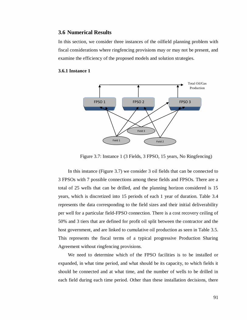
91


In this section, we consider three instances of the oilfield planning problem with

fiscal considerations where ringfencing provisions may or may not be present, and

examine the efficiency of the proposed models and solution strategies.

3.6.1 Instance 1

In this instance (Figure 3.7) we consider 3 oil fields that can be connected to

3 FPSOs with 7 possible connections among these fields and FPSOs. There are a

total of 25 wells that can be drilled, and the planning horizon considered is 15

years, which is discretized into 15 periods of each 1 year of duration. Table 3.4

represents the data corresponding to the field sizes and their initial deliverability

per well for a particular field-FPSO connection. There is a cost recovery ceiling of

50% and 3 tiers that are defined for profit oil split between the contractor and the

host government, and are linked to cumulative oil production as seen in Table 3.5.

This represents the fiscal terms of a typical progressive Production Sharing

Agreement without ringfencing provisions.

We need to determine which of the FPSO facilities is to be installed or

expanded, in what time period, and what should be its capacity, to which fields it

should be connected and at what time, and the number of wells to be drilled in

each field during each time period. Other than these installation decisions, there

FPSO 1 FPSO 3

Field 1

Field 3

Field 2

Total Oil/Gas

Production

FPSO 2

Figure 3.7: Instance 1 (3 Fields, 3 FPSO, 15 years, No Ringfencing)

92

are operating decisions involving the flowrate of oil, water and gas from each

field in each time period. The problem is solved to maximize the NPV of the

contractor’s share after paying taxes, and corresponding optimal investment and

operations decisions over the planning horizon.

Table 3.4: Field characteristics for instance 1

Fields Field Size

(MMbbl)

Initial Oil derivability per well (kstb/d)

FPSO 1 FPSO 2 FPSO 3

Field 1 230 16 18 16

Field 2 280 - 18 20

Field 3 80 15 - 12

Table 3.5: Sliding scale Contractor’s profit oil share for instance 1

Tiers Cumulative Oil Produced Contractor’s Share in Profit

Oil

Tier 1 0-150 MMbbl 50%

Tier 2 150-325 MMbbl 40%

Tier 3 >325 MMbbl 20%

The models are implemented in GAMS 23.6.3 and run on Intel Core i7, 4GB

RAM machine using CPLEX 12.2. The optimal solution of this problem is

presented in Table 3.6, that corresponds to Model 3F involving detailed

connections, suggests installing only FPSO 3 with a capacity 297.75 kstb/d and

161.90 MMSCF/d for liquid and gas, respectively, at the beginning of year 1. It

takes 3 years for this FPSO to be available for production. Fields 1 and 2 are

connected to this FPSO at the beginning of year 4, where 7 wells are drilled in

Field 1 and 6 wells are drilled in Field 2 to start the production. These fields are

preferred compared to Field 3 due to their large sizes and deliverabilities. Liquid

capacity of FPSO 3 facility is expanded by 103.93 kstb/d in year 5 that becomes

available in year 6 due to 1 year of lead time involved. Field 3 that is smaller in

size comes online at the beginning of year 6 when deliverability of fields 1 and 2

decreases, where 3 wells are drilled in this field with an additional well in year 9

when production goes down. There are no further expansions and well drillings

after year 9. Notice that most of the investments occur in early stages of the

93

project. The total NPV of this project is $ 1497.69M after paying government

share.

Table 3.6: Optimal Installation and Drilling Schedule for instance 1

Year 1 2 3 4 5 6 7 8 9 10-15

Facility

Installations

Install

FPSO3

- - - Expand

FPSO3

- - - - -

Field 1

- - - Drill

7 wells

- - - - - -

Field 2 - - - Drill

6 wells

Drill

1 well

Drill

2 wells

- - - -

Field 3 - - - - - Drill

3 wells

- - Drill

1 well

-

Figures 3.8-3.9 represent the total oil and gas flow rates for the FPSO facility

during the planning horizon considered. Given that the timing of the particular tier

activation depends upon the cumulative oil production for this instance (Table

3.5) Tier 2 becomes active after fifth year while Tier 3 is active after the eighth

year involving less share in profit oil for contractor, see Figure 3.10.

In contrast, the sequential approach that first maximizes NPV i.e. Model 3,

without considering the impact of the fiscal terms, and then calculates the

contractor share based on these decisions and fiscal rules, yields a very different

solution. The optimum in this case suggests installing FPSO3 with a large

capacity (liquid 445.54 kstb/d and gas 211.65 MMSCF/d) at the beginning of the

0

50

100

150

200

250

0 1 2 3 4 5 6 7 8 9 10 11 12 13 14 15

x (

kst

b/d

)

Year

Oil Flowrate for FPSO 3

0

50

100

150

200

0 1 2 3 4 5 6 7 8 9 10 11 12 13 14 15

g(M

MS

CF

/d)

Year

Gas Flowrate for FPSO 3

Figure 3.8: Total oil flowrate for FPSO 3 Figure 3.9: Total gas flowrate for FPSO 3

94

planning horizon without any future expansions. The drilling decisions are also

front ended compared to the solution of the fiscal model, Model 3F. However, the

total NPV of the contractor’s share in the sequential case turns out to be $

1362.67M, which is significantly lower than the optimal solution ($ 1497.69M) of

the model with fiscal considerations (Model 3F). These results represent the

optimistic nature of the sequential approach that tries to generate as much revenue

as possible at the beginning of the planning horizon neglecting the trade-offs that

are associated to the fiscal part. Therefore, it may lead to the decisions that can

incur large losses in the long term after considering the impact of the fiscal

calculations.

Table 3.7: Comparison of the computational performance of various models for

instance 1

Model

Solver # of

constraints

# of

continuous

variables

# of

discrete

variables

NPV

($Million)

Time

(s)

Model 2F

(MINLP)

BARON

9.0.6 3,557

2,236

345

1,198.44

(<60% gap)

>36,000

Model 3F

(MILP)

CPLEX

12.2 5,199 3,668 399 1,497.69 3,359

Model 3RF

(MILP)

CPLEX

12.2 5,147 3,570 322 1,497.69 337

0

50

100

150

200

250

300

350

400

450

500

550

600

650

0 1 2 3 4 5 6 7 8 9 10 11 12 13 14 15

Cu

mu

lati

ve

Oil

pro

du

ced

(M

Mbbl)

Year

Tier 1 Tier 2 Tier 3

Figure 3.10: Cumulative Oil Produced vs. Timing of Tier activation

95

Table 3.7 compares the computational performance of the various models. In

particular, Model 3RF which is obtained after binary reduction from Model 3F

yields the same solution in an order of magnitude less time (337s vs. 3,359s),

when solved to optimality. In contrast, solving the corresponding MINLP

formulation Model 2F with BARON 9.0.6 can only provide a solution having

NPV of $ 1198.44M with a 60% gap in more than 10 hours. Moreover, we

observe that solving Model 2F directly with DICOPT requires a good

initialization due to the additional binary variables and constraints that are added

in this fiscal model compared to Model 2. Therefore, the optimal solution from

corresponding MILP formulations (Model 3F and Model 3RF) provides a way to

obtain a near optimal solution of the original Model 2F. We fixed the design

decisions in Model 2F from the optimal solution of Model 3RF and solved the

resulting NLP problem that yields an NPV of $1496.26 M, which shows that the

accuracy of the MILP solution is within 0.1% of the MINLP formulation.

Therefore, the proposed MILP formulations are computationally efficient and

provide near optimal solutions. In the next section, we will use these MILP

models as the basis and examine the performance of the proposed computational

strategies for the larger instances.

3.6.2 Instance 2

(i) PSA without ringfencing provisions for Instance 2

Figure 3.11: Instance 2 (5 Fields, 3 FPSOs, 20 years, No ringfencing)

96

In this instance, we consider 5 oilfields that can be connected to 3 FPSOs

with 11 possible connections, see Figure 3.11. There are a total of 31 wells that

can be drilled in these 5 fields, and the planning horizon considered is 20 years.

There is a cost recovery ceiling of 50% and 4 tiers (see Fig. 3.3) that are defined

for profit oil fraction between the contractor and host government based on the

cumulative oil production. The problem is solved to maximize the NPV of the

contractor’s share after paying taxes and the corresponding optimal

investment/operations decisions.

Table 3.8 compares the performance of the MILP (Model 3F) involving

detailed connections and reduced MILP model (Model 3RF) that are the extension

of the Models 3 and 3R, respectively, with progressive PSAs. The models are

implemented in GAMS 23.6.3 and run on Intel Core i7, 4GB RAM machine using

CPLEX 12.2. We can observe that there is significant increase in the

computational time with fiscal consideration for the MILP formulation Model 3F

with this larger instance, which takes more than 10 hours with a 14% of

optimality gap as compared to the reduced MILP model (Model 3RF), which

terminates the search with a 2% gap in reasonable time.

Table 3.8: Computational Results for Instance 2 (Model 3F vs. Model 3RF)

Model

# of

constraints

# of

continuous

variables

# of

discrete

variables

NPV

($Million)

Time (s) Optimality

Gap

Model 3F 9,474 6,432 727 2,183.63 >36,000 <14%

Model 3RF 9,363 6,223 551 2,228.94 1,164 <2%

0

50

100

150

200

250

0 5 10 15 20

MM

SC

F/d

Year

0

100

200

300

400

500

600

700

0 5 10 15 20

kst

b/d

Year

Figure 3.12. Optimal liquid and gas capacities of FPSO 3 facility for Instance 2

(a) Liquid capacity (b) Gas capacity

97

The optimal solution from Model 3RF suggests installing 1 FPSO facility

(FPSO3) with expansions in the future (see Fig. 3.12), while Fig. 3.13 represents

the well drilling schedule for this example. The tiers 2, 3 and 4 for profit oil split

become active in years 6, 8 and 12, respectively, based on the cumulative oil

production profile during the given planning horizon. Notice that the optimal

solution of this problem fails to develop field 1, which is not intuitive. The reason

for not developing field 1 is that the size of the field 1 is quite small as compared

to the other fields and the superstructure we consider does not allow connecting

field 1 to FPSO 3, which is the only FPSO that is installed. Therefore, based on

the superstructure and field size, it is not worth to install an additional FPSO to

produce from this field after paying government share. In contrast, the solution

from the sequential approach suggests exploring field 1 as well since it is worth in

that case to install 2 small FPSO facilities and also produce from field 1 given that

the trade-offs due to fiscal rules are neglected. Whereas, the total NPV of the

contractor’s share in this case is lower than the optimal solution of Model 3RF

($1,914.71M vs. $2,228.94M ).Therefore, we can observe that incorporating fiscal

terms within development planning can yield significantly different investment

and operations decisions compared to a simple NPV based optimization.

Note that fiscal terms without tier structure, for instance fixed percentage of

profit share, royalty rates, often reduces the computational expense of solving the

deterministic model directly without any fiscal terms instead. Surprisingly, the

problem with flat 35% of the profit share of contractor is solved in 73s which is

0

2

4

6

8

10

0 5 10 15 20

Num

ber

of

Wel

ls

Year

f1

f2

f3

f4

f5

Figure 3.13. Optimal well drilling schedule for Instance 2

98

even smaller than the solution time for deterministic case without any fiscal terms

(190s). On the other hand, the problem with 2 tiers instead of 4 as considered

above is solved in 694s which is more than the model without fiscal terms and

less than the model with 4 tiers as can be seen in Table 3.9. Therefore, the

increase in computational time while including fiscal rules within development

planning, is directly related to the number of tiers (levels) that are present in the

model to determine the profit oil shares or royalties.

Table 3.9: Comparison of number of tiers vs. solution time for Model 3RF

# of tiers Time (s)

4 1,164

2 694

1 73

No fiscal rules 190

Table 3.10 compares the further improvements in the solution time for

Model 3RF (1,164s) after using the reformulation/approximation techniques and

strategies that are proposed. In particular, the tighter formulation Model 3RF-L

that is obtained after including logic constraint and valid inequalities, (3.65)-

(3.67), is solved in one fourth of the time than Model 3RF. Notice that these

MILP models are solved with a 2% of optimality tolerance yielding a slightly

different objective values for Model 3RF and Model 3RF-L. Model 3RI, which

relaxes the disjunction (3.30), can be solved more than 20 times faster than the

original Model 3RF. Although the solution obtained is a relaxed one (upper bound

of 2,591.10), it gives the optimal investment decisions that result in the same

solution as we obtained from solving Model 3RF directly. The approximate

version of this Model 3RI-A, takes only 82s as compared to Model 3RF (1164s)

and yields the optimal solution after we fix the decisions from this model in the

original one. Notice that the quality of the approximate solution itself is very good

(~1.5% accurate) and both relaxed/approximate models are even ~3 times faster

than the model without any fiscal terms (Model 3R) that takes 190s.

99

Table 3.10: Results for Instance 2 after using various solution strategies

Model # of

constraints

# of

continuous

variables

# of

discrete

variables

NPV

($Million)

NPV after

fixing

decisions in

Model 3RF

($Million)

Time (s)

Model 3RF 9,363 6,223 551 2,228.94 - 1,164

Model 3RF-L 11,963 6,223 551 2,222.40 - 275

Model 3RI-A 8,803 5,903 471 2,197.63 2,228.94 82

Model 3RI 8,803 5,903 471 2,591.10 2,228.94 48

(ii) PSA with ringfencing provisions for Instance 2

In this case, we consider two ringfences for the above Instance 2 (see Figure

3.4) where progressive PSA terms are defined for each of these ringfences

separately. Based on the computational performance of the Model 3RF as

compared to Model 3F in the previous case, we only show the results for Model

3RF, which is more efficient.

Table 3.11: Results for Instance 2 with ringfencing provisions

Model # of

constraints

# of

continuous

variables

# of

discrete

variables

NPV

($Million)

NPV

after

fixing

decisions

in Model

3RF

($Million)

Time

(s)

%

gap

Model 3RF 14,634 9,674 651 2,149.39 - >36,000 <15.4%

Model 3RF-L 19,834 9,674 651 2,161.27 - 3,334 <2%

Model 3RI-A 13,514 9,034 491 2,148.90 2,142.75 134 <2%

Model 3RI 13,514 9,034 491 2,533.06 2,151.75 112 <2%

Table 3.11 compares the results for various models for this case. We can

observe that including ringfencing provisions makes Model 3RF expensive to

solve (>10 hrs), compared to the previous instance without any ringfences that

required only 1,164s. This is due to the additional binary variables that are

required in the model for each of the two ringfences, their trade-offs and FPSO

cost disaggregation. In contrast, since Models 3RI and 3RI-A do not need binary

variable for the sliding scale in disjunction (3.30), they solve much faster than

Model 3RF (>300 times faster) and Model 3RF-L (~30 times faster). Notice that

even after including ringfencing provisions, these two models are faster than the

100

simple NPV based Model 3R. This is due to the trade-off from the fiscal part in

the simple NPV based model without binary variables for the sliding scale.

Notice that Model 3RI and 3RI-A are solved here in one of the most general

forms of the fiscal terms where the solutions may not be the global optimal, but

the relaxed Model 3RI, which provides a valid upper bound, also allows to

compare the solution quality. The optimal NPV after ringfencing provisions is

lower as compared to the earlier case without ringfencing provisions due to the

additional restrictions it imposes on the revenue and cash flows.

In addition, we also consider a bi-level decomposition approach (see

Appendix G) to solve this ringfencing instance. The algorithm considers an

aggregate fiscal model at upper level by neglecting the ringfencing provisions that

yields an upper bound ($2,222.40 M) as can be seen in Table 3.12. The lower

level detailed fiscal model is solved for the infrastructure selected from the upper

level problem to yield the feasible solution ($2,161.27 M). In the next iteration,

the upper level problem is solved with additional integer cuts that avoid the same

investment decisions to be selected. The objective value of this model ($2,040.23

M) becomes smaller than the lower bound obtained during the first iteration and

the algorithm stops. The MILP models are solved in this instance with a 2% of

optimality tolerance and total solution time is 869s. Based on these preliminary

results, the algorithm can be considered as an alternative to solve the oilfield

problems involving ringfencing provisions. However, the efficiency of the

algorithm relies on the efficiency of solving the lower and upper level problems

which may itself become expensive to solve for the large instances and/or may

need several iterations to close the gap.

Table 3.12: Bi-level decomposition for Instance 2 with ringfencing provisions

Iteration UB

($Million)

LB

($Million)

Optimality

gap

(%)

1 2,222.40 2,161.27 2.75%

2 2,040.23 - 0.00%

101

3.6.3 Instance 3

(i) PSA without ringfencing provisions for Instance 3

In this case, we consider a larger instance of the oilfield planning problem

with fiscal considerations. There are 10 oil fields (Figure 3.14) that can be

connected to 3 FPSOs with 23 possible connections. There are a total of 84 wells

that can be drilled in all of these 10 fields and the planning horizon considered is

20 years. There is a cost recovery ceiling of 50% and 4 tiers are defined for profit

oil split between the contractor and host government that are linked to cumulative

oil production. The objective is to maximize the NPV of the contractor’s share

after paying taxes and corresponding optimal investment/operations decisions.

Table 3.13: Results for Instance 3 after using various solution strategies

Model # of

constraints

# of

continuous

variables

# of

discrete

variables

NPV

($Million)

NPV after

fixing

decisions

in Model

3RF

($Million)

Time

(s)

%

gap

Model 3RF 17,640 11,727 963 6,440.58 - >72,000 <22%

Model 3RF-L 20,240 11,727 963 6,498.45 - 22,500 <10%

Model 3RI-A 17,080 11,407 883 6,355.00 6,452.36 2,035 <10%

Model 3RI 17,080 11,407 883 7,319.60 6,484.12 1,569 <10%

Field-9

FPSO-2 FPSO-3

Field-2

Field-1

Field-3 Field-5

FPSO-1

Field-4

Total Oil/Gas

Production

Field-10

Field-6

Field-8Field-7

Figure 3.14: Instance 3 with 10 Fields, 3 FPSO, 20 years

102

Table 3.13 compares the solution time required for Model 3RF with the

proposed reformulation/approximation techniques. We can observe that even

Model 3RF without any ringfences becomes expensive to solve for this larger

instance as compared to instance 2. Moreover, it takes more than 20hrs to reach

within 22% of optimality for Model 3RF, whereas the relaxed Model 3RI can be

solved in less than half an hour within 10% of optimality. The solution that is

obtained after fixing the design decisions in the original formulation is also better

than Model 3RF. Model 3RI-A, which is an approximation, also performs similar

to the relaxed model and gives an even improved solution than Model 3RF with a

~2% of accuracy. Both models are more than 20 times faster than even the tighter

formulation Model 3RF-L involving logic constraints and valid inequalities.

Surprisingly, these models perform again better than the model without any fiscal

terms, i.e. the simple NPV based model (Model 3R) takes more than 12,000s to

reach within 10% of optimality gap due to the trade-off that is missing between

production and fiscal part.

Notice that the times reported in Table 3.13 for Model 3RI-A and 3RI are the

times to solve Models 3RI-A and 3RI only. We did not include the time required

to solve Model 3RF with fixed decisions in all the examples considered since it

was negligible as compared to solution time of Models 3RI-A, 3RI and 3RF. For

instance, it is ~2 orders of magnitude smaller than the solution time required for

Model 3RI-A (25s vs. 2035s) for this case. It is due to the fact that the critical

discrete variables that represent the infrastructure and well drilling are fixed in the

model and most of the remaining decisions correspond to the continuous

operational decisions.

(ii) PSA with ringfencing provisions for Instance 3

In this case, we consider three ringfences for the above Instance 3 with 10

fields (see Figure 3.14) where Table 3.14 and 3.15 represent data corresponding

to the field sizes, ringfencing provisions and sliding scale profit oil divisions.

103

Table 3.14: Field Sizes and Ringfencing Provisions for Instance 3

Field F-1 F-2 F-3 F-4 F-5 F-6 F-7 F-8 F-9 F-10

Field Size

(MMbbl)

60 100 170 230 280 80 200 320 400 500

Corresponding

Ringfence

RF-1 RF-1 RF-1 RF-2 RF-2 RF-2 RF-3 RF-3 RF-3 RF-1

Table 3.15: Fiscal data for Instance 3 with ringfencing provisions

(i) Sliding scale Contractor’s Profit (ii) Tax rates and Cost Oil Ceilings

Oil share

Table 3.16 compares the computational results of various models for this

case of instance 3. It can be observed that including ringfencing provisions for

this largest instance makes even both Model 3RF and Model 3RF-L very

expensive compared to the previous case without any ringfences. This is due to

the additional binary variables that are required in the model for each of the three

ringfences separately and resulting weak relaxations.

Table 3.16: Results for Instance 3 with Ringfencing provisions

Model # of

constraints

# of

continuous

variables

# of

discrete

variables

NPV

($Million)

NPV after

fixing

decisions

in Model

3RF

($Million)

Time

(s)

%

gap

Model 3RF 33,403 22,150 1,163 6,382.46 - >72,000 <57%

Model 3RF-L 41,203 22,150 1,163 6,469.30 - >72,000 <22%

Model 3RI-A 31,723 21,190 923 6,273.59 6,442.68 3,383 <10%

Model 3RI 31,723 21,190 923 7,166.70 6,349.99 4,003 <10%

Ringfence

Income Tax Rate

( % of

Contractor's

Profit Oil Share)

Cost Recovery

Ceiling

(% of Gross

Revenues from

the Ringfence)

RF-1 30% 50%

RF-2 30% 50%

RF-3 30% 50%

Ringfences: RF-1, RF-2, RF-3

Cumulative oil

Produced

Contractor's

Profit Oil Share

Tier-1 0 - 200 MMbbl 50%

Tier-2 200 - 400 MMbbl 40%

Tier-3 400 - 600 MMbbl 30%

Tier-4 > 600 MMbbl 20%

104

In contrast, since Models 3RI and 3RI-A do not require binary variables for

sliding scales, they perform much better than Model 3RF and its tighter version

Model 3RF-L as observed in the earlier cases. Model 3RI is a relaxation and

yields a reasonable upper bound, while Model 3RI-A yields an approximate

solution within 3% of accuracy.

Figure 3.15 represents the optimal installation and connections between

fields and FPSO for this problem, where we can observe that each of the installed

FPSO (1 and 3) is connected to a total of 5 fields that do not belong to the same

ringfence. The optimal cumulative oil production profile for various ringfences is

shown in Figure 3.16, and the sliding scale rules in Table 3.15(i), results in the

different times of higher tier activations for these three ringfences as shown in

Table 3.17. Notice that ringfence 3, which involves larger size fields, enters into

higher tier (Tier 4) sooner as compared to the other ringfences. Moreover, in

ringfence 2 which has smaller fields, only 3 tiers become active.

Table 3.17: Optimal timings of Tier activations for various Ringfences

FPSO-3FPSO-1

Total Oil/Gas

Production

Field-2

Field-1

Field-3

Field-10

Field-8

Field-9Field-7

Field-5

Field-4

Field-6

Ringfence-1

Ringfence-2

Ringfence-3

Ringfence Tier-1 Tier-2 Tier-3 Tier-4

RF-1 Year 1- Year 6 Year 7- Year 8 Year 9- Year 12 Year 13- Year 20

RF-2 Year 1- Year 6 Year 7- Year 10 Year 11- Year 20 -

RF-3 Year 1- Year 6 Year 7- Year 8 Year 9- Year 11 Year 12- Year 20

Figure 3.15: Optimal Solution for Instance 3 with Ringfencing provisions

105

It is important to note that the performance of Models 3RI and 3RI-A is

independent of the number of ringfences that are present in the fiscal terms, as it

can be seen that the increase in solution time is negligible compared to the

previous case without ringfencing provisions. This is due to the fact that

increasing ringfences in these models only increases the number of continuous

variables and linear constraints, except a few binary variables that are required for

cost oil recovery calculation. In contrast, the complexity of Models 3RF and 3RF-

L that rely on disjunction (3.30) increases exponentially with an increase in the

number of ringfences or tiers. Moreover, it is also interesting to note that even

after including one of the extreme cases of the fiscal term (progressive PSA with

ringfencing) for a large instance involving 10 fields, the proposed

relaxed/approximate models still perform extremely well, and they are in fact

even 3-4 times better than the simple NPV based Model 3R without fiscal

considerations.

3.7 Conclusions

In this chapter, we have introduced the fiscal aspects within offshore oil and gas

field planning problem. These fiscal considerations are usually either ignored or

0

100

200

300

400

500

600

700

800

900

0 1 2 3 4 5 6 7 8 9 10 11 12 13 14 15 16 17 18 19 20

Cu

mu

lati

ve O

il P

ro

du

ced

(M

Mb

bl)

Year

Cumulative Oil Production Profile for various Ringfences

Ringfence-1

Ringfence-2

Ringfence-3

Figure 3.16: Optimal Cumulative Oil production for Instance 3 with Ringfencing provisions

106

considered in an ad-hoc manner, which may have a very large impact on the

planning decisions. In particular, we have proposed a general model for the multi-

field site problems that accounts for the fiscal calculations in the objective

functions and constraints explicitly. The model is an extension of the

strategic/tactical planning model presented in the previous chapter to progressive

PSAs involving ringfencing provisions. Few simpler cases of the fiscal contracts

have also been derived from the proposed general model as an illustration. The

model yields investment and operating decisions that are not only optimal in the

sense of NPV after taxes for the project at hand, but also provides a more

appropriate basis to compare a portfolio of different projects involving different

fiscal contracts and other details. However, as the computational expense can be a

serious issue with the incorporation of fiscal terms for some particular contract,

we have also proposed a tighter formulation using additional logic constraints and

valid inequalities, two heuristic approaches yielding good solutions to the large

instances, and a bi-level decomposition approach. Numerical results in realistic

examples show that these models and solution strategies are quite efficient, and

reduce the solution time orders of magnitude than using the MILP for the

disjunctive formulation. We hope that this work has shown that explicit

consideration of the fiscal rules is important for oilfield infrastructure planning,

and that the models/methods described here can serve as the basis for further

extensions and improvements in the computational effort.

107

Chapter 4

Solution strategies for multistage

stochastic programming with

endogenous uncertainties in the

planning of process networks

4.1 Introduction

In this chapter, we consider a general multistage stochastic mixed-integer linear

programming model for multiperiod planning problems where optimization

decisions determine the times when the uncertainties in some of the parameters

will be resolved, i.e. decision-dependent uncertainty (Jonsbraten et al., 1998; Goel

and Grossmann, 2006; and Tarhan and Grossmann, 2008). To address the issue of

computational expense in solving these endogenous uncertainty problems, we also

present several solution strategies and apply them to process network examples

having uncertainty in the process yields which can only be revealed once an

investment is made in the process.

The outline of this chapter is as follows. First, in sections 4.2 and 4.3 we

present the problem statement for the endogenous uncertainty problems under

consideration and the corresponding multistage stochastic programming model,

respectively. In section 4.4, three theoretical properties are identified for the

model and used to formulate a reduced model in the subsequent section. To solve

the large instance of the problems in this class a k-stage constraint solution

approach, NAC relaxation strategy, and a Lagrangean decomposition algorithm

108

are proposed in section 4.6. The proposed models and solution strategies are then

applied to two process network problems under uncertain yields in section 4.7 to

illustrate the advantages of these approaches.


In the class of problems under consideration, the time horizon is represented by

the discrete set of time periods T = {1, 2, . . . . }. Set I = {1, 2, . . . .} represents the

set of “sources” of endogenous uncertainty, while θi represents the endogenous

uncertain parameter associated with source . The discrete set of possible

realizations for θi is represented by Φi. The resolution of uncertainty in θi depends

on the binary decision variables bi,t. Specifically, the uncertainty in θi will be

resolved in time period t if binary decision bi,t = 1 and bi,τ = 0, τ < t. Note that

the parameters θi represent intrinsic properties of source i and are assumed to be

independent and time invariant. Besides the decisions represented by variables bi,t,

other decisions to be made in time period t are represented by variables yt and xt

where these are decisions made at the beginning and end of the corresponding

time period t.

The sequence of events in each time period is as follows. Decisions yt and bi,t

are implemented at the beginning of time period t . This is followed by the

resolution of uncertainty in the endogenous parameter θi for source i if bi,t = 1 and

bi,τ = 0 τ < t. The state variables ( tw ) are calculated based on the decision

variables that are selected, while the recourse variables ( tx ) are decisions

implemented at the end of each period.

In general, the variables bi,t may represent investment decisions associated

with source i. In the gas field problem considered by Goel et al. (2006), these

variables represent whether or not investment is made at field i in time period t.

The uncertainty associated with a field is resolved in time period t only if

investment is carried out at that field in time period t, while no investments have

been made at that field in the past. Similarly, for capacity expansion planning

problems these decisions represent whether or not unit i is installed in time period

t. However, in this case we assume that the uncertainty associated with a process

109

gets resolved as soon as initial investment is made in that process and it is

independent of the plant capacity.

Note that for ease of exposition, we assume that there is only one

endogenous uncertain parameter associated with source i for all . Thus, θi is a

scalar for all . Moreover, the problem statement presented here is the specific

case of the one that is described in Goel and Grossmann (2006).

4.3 Model

The multistage stochastic programming model (MSSP0) with endogenous

uncertainty can be represented as a mixed-integer linear disjunctive programming

model as described in Goel and Grossmann (2006).

(MSSP0)

Tt Ii

s

ti

bs

ti

s

t

ys

t

s

t

xs

t

s

t

ws

t

Ss

s bcycxcwcp ,,min

(4.1)

s

t

tT Ii

s

i

bs

ti

sys

t

sxs

t

sws

t abAyAxAwAts

,

,,,,,,.. TtSs , (4.2)

s

i

s

i bb

1,1, ',,, ssIiSss (4.3a)

ss yy

11 ',', ssSss (4.3b)

',,, ssTtSss (4.4)

}1,0{,,, , s

ti

s

t

s

t

s

t

s

t

s

t

s

t bYyXxWw IiTtSs ,,

},{', FalseTrueZ ss

t TtSss ,,

The objective function (4.1) in the above model (MSSP0) minimizes the

expectation of an economic criterion. For a particular scenario, inequality (4.2)

represents constraints that govern decisions in time period t and link decisions

across time periods. First time period non-anticipativity (NA) constraints are

(4.5) ',

11

1,1,

',

ss

t

s

t

s

t

s

ti

s

ti

s

t

s

t

ss

t

Z

yy

Iibb

xx

Z

)( ,1)',(

', s

i

t

ssDi

ss

t bZ

',,, ssTtSss

110

given by equations (4.3a) and (4.3b), while conditional NA constraints that are

written for the later time periods in terms of decisions s

tib , are given by (4.4) and

(4.5). Note that the set D(s,s’) that is used in the equation (4.4) is defined as

follows:

',)',( s

i

s

iIiissD

The idea of non-anticipativity is that the decisions at time t can only be

affected by the decisions ( s

ti

s

t by ,, ) made before time period t. These constraints

state that if two scenarios s and s’ are indistinguishable in time period t (i.e. they

are the same), then decisions for these scenarios in time period t should be the

same. It should also be noted that problem (MSSP0) can be reformulated as an

MILP as described in Goel and Grossmann (2006) by replacing the equations

(4.4) and (4.5) with integer and mixed-integer constraints, respectively.

4.4 Model Reduction Scheme

NA constraints like the ones in (4.3a), (4.3b) and (4.5) are essential in multistage

stochastic programming to ensure that our current decisions do not anticipate

future outcomes. When the model (MSSP0) is reformulated as an MILP problem,

the difficulty is that the NA constraints typically represent around 80% of the total

constraints and grow quadratically in the number of scenarios, making real-world

size problems intractable. To overcome this limitation, we present three

theoretical properties that allow us to formulate significantly reduced MSSP

models.

Let us assume that there are p uncertain parameters (θ1, θ2, θ3,.........., θp)

each of which has k realizations (l1, l2, l3,.........., lk ). Then the total number of

combinations of realizations of these parameters will be pk each of which will

define a scenario s. For these pkS scenarios there will be a total of )1( SS

scenario pairs (s, s’) each of which corresponds to a NA constraint in each time

period t. The following properties significantly reduce the problem size by

reducing the number of these scenario pairs (s, s’) and the corresponding NA

111

constraints. The first two properties were proposed by Goel and Grossmann

(2006).

Property 1. If scenario pair (s, s’) is indistinguishable at stage t, so is (s’, s).

Therefore, we have to consider only one of these scenario pairs (i. e. (s, s’) such

that s < s’).

Proof. See Goel and Grossmann (2006).

Property 2. It is sufficient to express NA constraints for the pairs of scenarios (s,

s’) that differ in the outcome of only one uncertain parameter.

Proof. See Goel and Grossmann (2006).

Property 1 is based on the symmetry of the scenario pairs (s, s’) and prevents

duplication of the NA constraints for the same pair of scenarios (s, s’) in the

model. On the other hand, Property 2 exploits the fact that the NA constraints

between those scenarios which differ in the realizations of more than one

uncertain parameter is implicitly enforced by considering the NA constraints for

the one that differ in realization of only one uncertain parameter. Therefore, it is

sufficient to include a subset of scenario pairs corresponding to those that differ in

realization of one uncertain parameter. Properties 1 and 2 are further illustrated by

a small example in the next section. Although, these two properties significantly

reduce the number of scenario pairs for the NA constraints, there are still many of

these scenario pairs that are connected implicitly and that can be removed. This

motivates us to find these scenario pairs systematically to further reduce the size

of the problem and establish a new Property 3.

Property 3 basically exploits transitivity relationship among scenario pairs (s,

s’) that results after applying Properties 1-2, and is an extension of Property 2 to

those cases where uncertain parameters have more than two realizations (i.e. k

>2). In that case, according to the Property 2 all the scenario pairs that differ in

just one uncertain parameter will be included in the model for the NA constraints

and there will be multiple links among those scenarios pairs that corresponds to a

single uncertain parameter. Some of these multiple links among scenarios are not

needed because of the fact that many of these scenarios that corresponds to a

single uncertain parameter are such that they can be only realized at the same time

112

irrespective of any decisions taken during the planning horizon and hence, we can

take advantage of the transitivity relation among these scenarios.

Therefore, the new property establishes that for an endogenous uncertainty

problem with p uncertain parameters and each having k realizations, it is

sufficient to express NA constraints only for those scenario pairs (s, s’) such that

,),....,,()',( 21 ksssss where pk Lsss ),....,,( 21 for each uncertain parameter θp

and s, s’ are the consecutive elements in this set. The required set pL is defined as

follows:

pssssspssD

sssSssssssL

k

kkk

p

),...,,()',(}{)',(

,...,,...,,),...,,(

21

212121

The k scenarios within each of these ),....,,( 21 ksss sets can only be realized at

the same time irrespective of the other realizations during the given time horizon

because they differ in the realization of the same uncertain parameter θp.

Therefore, unique linking among only these scenarios will be sufficient to enforce

non-anticipativity. Specifically, Property 3 can be stated as follows:

Property 3. For an endogenous uncertainty problem having p uncertain

parameters and S scenarios, the maximum number of scenario pairs (s, s’)

required to represent the non-anticipativity are )(/1 pp

SSp

.

Proof. Suppose that for an endogenous uncertainty problem,

p is the number of uncertain parameters = (θ1, θ2, θ3,.........., θp)

k is the number of realizations of each uncertain parameter

= (l1, l2, l3,.........., lk )

Therefore, the total number of scenarios are S = pk

For each uncertain parameter θp, there will be a total of 1pk number of

scenario sets ),....,,( 21 ksss , i.e.1 p

p kL , each having k scenarios. The

characteristic of these k scenarios within a set pk Lsss ),....,,( 21 is that uncertainty

in these scenarios can be realized at the same time irrespective of the other

realization during the specified time horizon because these scenarios have the

same realizations for all the uncertain parameters except for that particular

113

uncertain parameter θp. In other words, the k scenarios in a set pk Lsss ),....,,( 21

differ only in the realization of the uncertain parameter θp and can be realized at

the same time irrespective of other realizations. Also, according to Property 2, it is

sufficient to express NA constraints for those scenario pairs that differ in the

realization of only one uncertain parameter. Therefore, we do not need to include

scenario pairs (s, s’) that differ in realization of more than one uncertain

parameter. As the uncertainty in these k scenarios in a set ),....,,( 21 ksss is realized

at same time, it is sufficient to express non-anticipativity uniquely in these k

scenarios only. Hence, 1k scenario pairs (s, s’) will be required to link k

scenarios in each of these sets ),....,,( 21 ksss , i.e. 1k equations are required to

represent non-anticipativity for each of these 1pk number of sets for a particular

uncertain parameter θp. Therefore, the total number of scenario pairs (s, s’)

required for non-anticipativity are )1(1 kpk p

or )(/1 pp

SSp

. □

The proposed Property 3 can be used in addition to earlier Properties 1 and 2

to reduce the model size as explained in the next section with a small example.

Qualitatively, the end result of using these 3 properties is that they lead to the

minimum number of independent links between the scenarios to represent the NA

constraints.

4.5 Reduced Model Formulation

In this section we apply the three properties described above in order to reduce the

size of the model (MSSP0). Let us define,

P: Set of scenario pairs (s, s’) for NACs in the model (MSSP0)

P1: Set of scenario pairs (s, s’) for NACs after applying Property 1

P2: Set of scenario pairs (s, s’) for NACs after applying Properties 1 and 2

P3: Set of scenario pairs (s, s’) for NACs after applying Properties 1,2 and 3

Therefore,

',',)',( ssSssssP

',',)',(1 ssSssssP

1)',(,',',)',(2 ssDssSssssP

114

pLsssssssssP pkkk ),...,,(),(),....,,(),,( 21132213

The relation between these sets can be stated as, PPPP 123 .

The reduced model (MSSPR) that is formulated from the original model

(MSSP0) by considering NA constraints for scenario pairs (s, s’) within the set P3

for the equations (4.3a), (4.3b), (4.4) and (4.5) is given as follows:

(MSSPR)

Tt Ii

s

ti

bs

ti

s

t

ys

t

s

t

xs

t

s

t

ws

t

Ss

s bcycxcwcp ,,min (4.1)

s

t

tT Ii

s

i

bs

ti

sys

t

sxs

t

sws

t abAyAxAwAts

,

,,,,,,.. TtSs , (4.2)

IiPss ,),( 3 (4.6a)

3),( Pss (4.6b)

TtPss ,),( 3 (4.7)

(4.8)

IiTtSs ,,

TtSss ,,

Theorem 4.1. The optimum solution of the Reduced model (MSSPR) is the same

as the optimum solution of the Original Model (MSSP0).

The proof follows trivially from applying Properties 1-3. To illustrate the

effect of the proposed properties on the problem size, we consider a case of

endogenous uncertainty problem having 2 uncertain parameters, i.e. (θ1, θ2). Each

of these uncertain parameters has three realizations (l1, l2, l3) which give rise to a

total of 9 scenarios shown in Table 4.1.

)( ,1)',(

', s

i

t

ssDi

ss

t bZ

',

11

1,1,

',

ss

t

s

t

s

t

s

ti

s

ti

s

t

s

t

ss

t

Z

yy

Iibb

xx

Z

},{

}1,0{,,,

',

,

FalseTrueZ

bYyXxWw

ss

t

s

ti

s

t

s

t

s

t

s

t

s

t

s

t

TtPss ,),( 3

s

i

s

i bb

1,1,

ss yy

11

115

According to the original model (MSSP0), a total of 72 scenario pairs will be

required to represent non-anticipativity in the above problem as shown in Table

4.2(a) where each element in the table represent the indices of uncertain

parameters, (θ1, θ2) that differentiate the corresponding scenarios s and s’, i.e. set

D(s, s’).

However, if we use Property 1 (i.e. (s, s’) such that s < s’) the number of

scenario pairs reduces to 36 from 72 due to the symmetry of the scenario pairs as

seen in Table 4.2(b). Now, if we apply Property 2 (i.e. consider the scenario pairs

which differ in realization of only one uncertain parameter) then (s, s’) becomes

18 by removing those scenario pairs have more than one element in the set D(s,

s’) as seen in Table 4.2(c). But out of these 18 scenario pairs, only 12 are

sufficient as seen in Table 4.2(d) to uniquely define the non-anticipativity that

also satisfies the requirement of Property 3. This is due to the transitivity relation

among the scenarios pairs corresponding to a single uncertain parameter and their

characteristic of being realized at the same time irrespective of the other decisions

as explained in the previous section. Hence, there is 83.33% reduction (i.e. from

72 to 12) in the scenario pairs (or problem size) on using the three theoretical

properties. Note that for this example L1 = {(s1, s2, s3), (s4, s5, s6), (s7, s8, s9)} and

L2 = {(s1, s4, s7), (s2, s5, s8), (s3, s6, s9)} according to the definition of these sets

described earlier.

Scenario (s) 1 2 3 4 5 6 7 8 9

θ1 l1 l2 l3 l1 l2 l3 l1 l2 l3

θ2 l1 l1 l1 l2 l2 l2 l3 l3 l3

Table 4.1: 9 Scenarios for the given example

116

Table 4.2: Scenario pairs and corresponding differentiating set D(s, s’) for the 9 scenario example

D(s,s’) 1 2 3 4 5 6 7 8 9

1 1 1 2 1,2 1,2 2 1,2 1,2

2 1 1 1,2 2 1,2 1,2 2 1,2

3 1 1 1,2 1,2 2 1,2 1,2 2

4 2 1,2 1,2 1 1 2 1,2 1,2

5 1,2 2 1,2 1 1 1,2 2 1,2

6 1,2 1,2 2 1 1 1,2 1,2 2

7 2 1,2 1,2 2 1,2 1,2 1 1

8 1,2 2 1,2 1,2 2 1,2 1 1

9 1,2 1,2 2 1,2 1,2 2 1 1

D(s,s’) 1 2 3 4 5 6 7 8 9

1 1 1 2 1,2 1,2 2 1,2 1,2

2

1 1,2 2 1,2 1,2 2 1,2

3

1,2 1,2 2 1,2 1,2 2

4

1 1 2 1,2 1,2

5

1 1,2 2 1,2

6

1,2 1,2 2

7

1 1

8

1

9

D(s,s’) 1 2 3 4 5 6 7 8 9

1 1 1 2 2

2 1 2 2

3 2 2

4 1 1 2

5 1 2

6 2

7 1 1

8 1

9

D(s,s’) 1 2 3 4 5 6 7 8 9

1 1 2

2 1 2

3 2

4 1

2

5 1 2

6 2

7 1

8 1

9

(a) 72 Scenario pairs in the original model (MSSP0)

(b) 36 Scenario pairs after using Property 1

(c) 18 Scenario pairs after using Properties 1-2 (d) 12 Scenario pairs after using Properties 1-3

117

The graphical illustration of the model reduction scheme for the above 9

scenario example can be seen in Figure 4.1. Property 1 basically removes one of

the two links between scenarios 1 and 2 in the figure. Scenarios 1 and 5 differ in

both the uncertain parameters and due to the implicit connection between these

scenarios through links 1-2 and 2-5 each of which corresponds to a single

uncertain parameter, Property 2 can be used to remove the link 1-5. Because

scenarios 1, 4 and 7 differ in the realization of just the second uncertain parameter

θ2 and can only be realized simultaneously, they can be expressed by unique link

among them. Therefore, Property 3 removes the link 1-7 and still allowing

scenarios 1 and 7 to take non-anticipative decisions through the links 1-4 and 4-7.

The other similar links removed by these properties are not shown in the figure

for clarity.

Property 3 can be easily extended to the cases where there is a different

number of realizations for each uncertain parameter. In that case, we need to

create some dummy realizations for some of the uncertain parameters to make the

same number of realizations for all the uncertain parameters and apply Property 3

to find out the least number of scenario links required for this new scenario set.

Figure 4.1: Model Reduction Scheme for 9 scenario example

118

Finally, we can remove those scenario pairs from the NA constraints set that

involve dummy realizations of the uncertain parameters leading to the least

number of NA constraints for the given realizations.

Note that the number of scenario pairs using Properties 1-3 will be smaller

compared to using Properties 1-2 only if the number of realization of uncertain

parameters is more than two. Otherwise we will get the same number of scenarios

in both cases. Therefore, in contrast to the earlier properties by Goel and

Grossmann (2006), the proposed Property 3 can be regarded as the extension of

the Property 2 to the cases where uncertain parameters have more than two

realizations. Moreover, the effect of these properties on the problem size and

solution time becomes very significant for the problems having large number of

scenarios and/or having many realizations of each uncertain parameter.

4.6 Solution Strategies

Although the model formulation in the previous section greatly reduces the size of

the multistage stochastic programs with endogenous uncertainties, given the

exponential increase in the problem size with the number of uncertain parameters

and its realizations, these problems may not be solvable in reasonable

computational time. Hence, we may need some special solution techniques to

solve large-scale problems in this class as discussed in this section.

4.6.1 k-stage Constraint Strategy

We know that NA constraints play a major role in the size of any multistage

stochastic program and most of them are inactive at the optimum solution of the

problem, particularly in the later time periods since investments tend to take place

in the earlier periods. This observation motivates us to include only the subset of

these constraints, corresponding up to the first k-stages of the problem which are

assumed to be critical for defining the optimum solution of the problem. By

defining ST as the set of k initial stages for which NA constraints are to be

included, the proposed k-stage constraint formulation that is obtained from the

reduced model by replacing the set T with ST in equations (4.7) and (4.8) is as

follows:

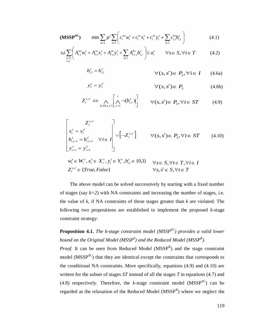
119

(MSSPSC

)

Tt Ii

s

ti

bs

ti

s

t

ys

t

s

t

xs

t

s

t

ws

t

Ss

s bcycxcwcp ,,min (4.1)

s

t

tT Ii

s

i

bs

ti

sys

t

sxs

t

sws

t abAyAxAwAts

,

,,,,,,.. TtSs , (4.2)

IiPss ,),( 3 (4.6a)

3),( Pss (4.6b)

STtPss ,),( 3 (4.9)

STtPss ,),( 3 (4.10)

The above model can be solved successively by starting with a fixed number

of stages (say k=2) with NA constraints and increasing the number of stages, i.e.

the value of k, if NA constraints of those stages greater than k are violated. The

following two propositions are established to implement the proposed k-stage

constraint strategy:

Proposition 4.1. The k-stage constraint model (MSSPSC

) provides a valid lower

bound on the Original Model (MSSP0) and the Reduced Model (MSSP

R).

Proof. It can be seen from Reduced Model (MSSPR) and the stage constraint

model (MSSPSC

) that they are identical except the constraints that corresponds to

the conditional NA constraints. More specifically, equations (4.9) and (4.10) are

written for the subset of stages ST instead of all the stages T in equations (4.7) and

(4.8) respectively. Therefore, the k-stage constraint model (MSSPSC

) can be

regarded as the relaxation of the Reduced Model (MSSPR) where we neglect the

',

11

1,1,

',

ss

t

s

t

s

t

s

ti

s

ti

s

t

s

t

ss

t

Z

yy

Iibb

xx

Z

},{

}1,0{,,,

',

,

FalseTrueZ

bYyXxWw

ss

t

s

ti

s

t

s

t

s

t

s

t

s

t

s

t

)( ,1)',(

', s

i

t

ssDi

ss

t bZ

IiTtSs ,,

TtSss ,,

s

i

s

i bb

1,1,

ss yy

11

120

conditional NA constraints for the stages that are not the elements of the set ST.

Hence, the k-stage constraint model (MSSPSC

) provides a valid lower bound on

the Reduced Model (MSSPR). As models (MSSP

R) and (MSSP

0) are equivalent,

the k-stage constraint model (MSSPSC

) also provides a valid lower bound on the

Original Model (MSSP0). □

Proposition 4.2. The k-stage constraint model (MSSPSC

) provides the optimum

solution to the Original Model (MSSP0) and the Reduced Model (MSSP

R), if there

is no realization of any of the endogenous uncertain parameter after specified

stages in the solution that is obtained.

Proof. The proof follows from the fact that if there is no realization of any of the

uncertain parameter after specified stage k in the solution, then there will be no

new information available to any scenario from period k +1 to end of the planning

horizon T. Therefore, the state of the system corresponding to each scenario will

be the same from period k to T. Moreover, the scenario pairs that have already

being distinguished within the first k stages according to the logic condition of the

non-anticipativity, there will not be any need to include NA constraints for these

scenario pairs. On the other hand, if there are some scenario pairs that have not

been distinguished until stage k, and as there in no further realization of

uncertainty, these scenarios will have the same information from period 1 to T and

will have the same decisions. Hence, the NA constraints from period k+1 to T

will automatically be satisfied for these scenario pairs. Given that the reduced

model (MSSPR) and the stage constraint model (MSSP

SC) are identical except the

conditional NA constraints that were relaxed, i.e. from period k+1 to T in the

stage constraint model, and because the NA from period k+1 to T are satisfied in

the solution of k stage constraint model if there is no realization of uncertain

parameter after stage k as discussed earlier, the solution of the stage constraint

model corresponding to the current stage k will be the optimum solution for the

reduced model (MSSPR). As models (MSSP

R) and (MSSP

0) are equivalent, the k-

stage constraint model (MSSPSC

) also provides an optimal solution to the Original

Model (MSSP0) if the above condition is satisfied. □

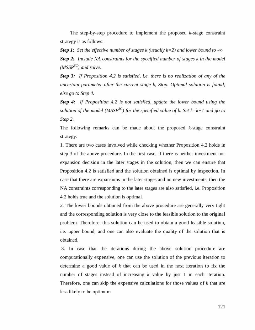
121

The step-by-step procedure to implement the proposed k-stage constraint

strategy is as follows:

Step 1: Set the effective number of stages k (usually k=2) and lower bound to -∞.

Step 2: Include NA constraints for the specified number of stages k in the model

(MSSPSC

) and solve.

Step 3: If Proposition 4.2 is satisfied, i.e. there is no realization of any of the

uncertain parameter after the current stage k, Stop. Optimal solution is found;

else go to Step 4.

Step 4: If Proposition 4.2 is not satisfied, update the lower bound using the

solution of the model (MSSPSC

) for the specified value of k. Set k=k+1 and go to

Step 2.

The following remarks can be made about the proposed k-stage constraint

strategy:

1. There are two cases involved while checking whether Proposition 4.2 holds in

step 3 of the above procedure. In the first case, if there is neither investment nor

expansion decision in the later stages in the solution, then we can ensure that

Proposition 4.2 is satisfied and the solution obtained is optimal by inspection. In

case that there are expansions in the later stages and no new investments, then the

NA constraints corresponding to the later stages are also satisfied, i.e. Proposition

4.2 holds true and the solution is optimal.

2. The lower bounds obtained from the above procedure are generally very tight

and the corresponding solution is very close to the feasible solution to the original

problem. Therefore, this solution can be used to obtain a good feasible solution,

i.e. upper bound, and one can also evaluate the quality of the solution that is

obtained.

3. In case that the iterations during the above solution procedure are

computationally expensive, one can use the solution of the previous iteration to

determine a good value of k that can be used in the next iteration to fix the

number of stages instead of increasing k value by just 1 in each iteration.

Therefore, one can skip the expensive calculations for those values of k that are

less likely to be optimum.

122

The proposed k-stage constraint strategy can be quite effective for the

investment planning models because the trend in problems of this class is that

their optimum solution involves investments in the earlier stages of the project.

The reason behind this is the effect of economies of scale, as in general, it pays to

make investments only once and earlier because of the fixed cost charges. Second,

if one expands the capacity, it is better to do it early as otherwise one will not take

full advantage of the investment. This implies that the investment and operation

decisions in the early stages of planning horizon are critical for these problems

and require enforcing the NA constraints in these stages, while the ones for later

stages can be ignored making the large-scale investment planning problems easier

to solve. Specific examples for these problems are process network planning, or

oil and gas fields infrastructure planning problems.

4.6.2 NAC Relaxation Strategy

The k-stage constraint strategy presented in the previous section involves the

solution of the reduced model for the specified number of stages iteratively and

has advantage for the investment planning problems where only first few stages

involve uncertainty realization. This is due to the economies of scale in these

problems as explained earlier. On the other hand, if there are endogenous

uncertainties that are revealed later in the planning horizon, then the stage

constraint approach can become expensive for finding the optimal solution due to

the solution of MILP problems for multiple times, although a strong lower bound

to the problem can still be obtained.

Therefore, for the more general problems we propose a NAC relaxation

strategy. This strategy is motivated by the fact that very few inequality NA

constraints become active at the optimal solution of the problem (e.g. see Colvin

and Maravelias, 2010). In this strategy (Figure 4.2), we divide the solution

procedure in two phases, Phase I and Phase II. Phase I involves removing all

inequality NA constraints from the reduced model (MSSPR) and solving its LP

relaxation (LP-MSSPR). Then we check the feasibility of the NA constraints and

add the violated NA constraints in the LP relaxation and solve iteratively until

there is no violation of the NA constraints in the LP relaxation. In Phase II of the

123

NAC relaxation strategy, the resulting model from Phase I with the added cuts is

solved as an MILP problem to obtain a lower bound that is usually very tight. The

upper bound is obtained by fixing the binary decisions in the reduced model

(MSSPR) using the solution of the lower bounding MILP problem such that NA

constraints are not violated and solving the problem in fullspace. If the gap

between lower and upper bounds is more than the specified tolerance, we check

the feasibility of the NA constraints for the MILP solution in the current iteration

and solve the new MILP problem with violated NA constraints that serve as

added cuts in the next iteration. The procedure of solving lower and upper

bounding problems in Phase II continues until the gap between upper and lower

bound is within the specified optimality tolerance.

Note that in comparison to the branch and cut solution method by Colvin and

Maravelias (2010), the proposed NAC relaxation strategy is much easier to

implement directly using the available commercial solvers, although there might

be some trade-offs between these solution strategies in terms of the solution

times. Furthermore, it has been observed that very few inequality NA constraints

(~6-7% of the total inequality NA constraints in the reduced model) are added as

cuts in the complete solution procedure and most of the violated NA constraints

Figure 4.2: NAC Relaxation Strategy

No

Yes

Yes

No

Phase II

Phase I

Solve LP-MSSPR

NAC feasible

Solve MILP with added

NAC’s and update LB

Solve Reduced Model (MSSPR)

with fixed 0-1 variables

Feasible Solution

Solve Reduced Model (MSSPR) with fixed

0-1 variables such that NAC’s are feasible

Yes

No

Add violated

NAC’s

Add violated

NAC’s

Update UB and check

if UB-LB < ɛ

Stop

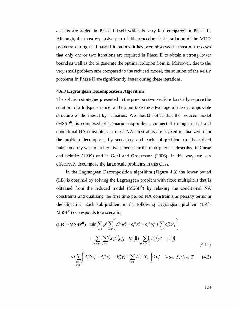
124

as cuts are added in Phase I itself which is very fast compared to Phase II.

Although, the most expensive part of this procedure is the solution of the MILP

problems during the Phase II iterations, it has been observed in most of the cases

that only one or two iterations are required in Phase II to obtain a strong lower

bound as well as the to generate the optimal solution from it. Moreover, due to the

very small problem size compared to the reduced model, the solution of the MILP

problems in Phase II are significantly faster during these iterations.

4.6.3 Lagrangean Decomposition Algorithm

The solution strategies presented in the previous two sections basically require the

solution of a fullspace model and do not take the advantage of the decomposable

structure of the model by scenarios. We should notice that the reduced model

(MSSPR) is composed of scenario subproblems connected through initial and

conditional NA constraints. If these NA constraints are relaxed or dualized, then

the problem decomposes by scenarios, and each sub-problem can be solved

independently within an iterative scheme for the multipliers as described in Carøe

and Schultz (1999) and in Goel and Grossmann (2006). In this way, we can

effectively decompose the large scale problems in this class.

In the Lagrangean Decomposition algorithm (Figure 4.3) the lower bound

(LB) is obtained by solving the Lagrangean problem with fixed multipliers that is

obtained from the reduced model (MSSPR) by relaxing the conditional NA

constraints and dualizing the first time period NA constraints as penalty terms in

the objective. Each sub-problem in the following Lagrangean problem (LRR-

MSSPR) corresponds to a scenario:

(LRR -MSSP

R)

(4.11)

s

t

tT Ii

s

i

bs

ti

sys

t

sxs

t

sws

t abAyAxAwAts

,

,,,,,,.. TtSs , (4.2)

33 )',(

'

11

',

1,

'

1,1,

',

1,,

)',(

,,min

Pss

ssss

y

Ii

s

i

s

i

ss

ib

Pss

Tt Ii

s

ti

bs

ti

s

t

ys

t

s

t

xs

t

s

t

ws

t

Ss

s

yybb

bcycxcwcp

125

1,0,,, , s

ti

s

t

s

t

s

t

s

t

s

t

s

t bYyXxWw

IiTtSs ,,

The upper bound (UB) is generated by using a heuristic based on the solution

of the Lagrangean problem. In this heuristic, we fix the decisions obtained from

the above problem (LRR- MSSP

R) in the reduced problem (MSSP

R) such that

there is no violation of NA constraints and solve it to obtain the upper bound. The

sub-gradient method by Fisher (1985) is used during each iteration to update the

multipliers for the Lagrangean problem. The algorithm stops when either a

maximum iteration limit is reached, or the difference between the bounds LB and

UB is less than a pre-specified tolerance.

The major advantage with the above Lagrangean decomposition algorithm

for endogenous uncertainty problems is that it provides good bounds on the

optimal solution at the root node by taking advantage of the decomposable

structure of the problem. Notice that in contrast to the method presented by Goel

and Grossmann (2006), no branch and bound method is performed here with

which the dual gap may not be closed for the problem. Therefore, if the gap

between lower and upper bounds is large then in principle we would have to also

Initial Multipliers (λ0)

and iteration no. k = 0

LB = -∞

UB = ∞

Yes

Solve Lagrangean subproblem

with fixed multipliers to get LB

Gap < ε

or k > kmax

Stop

Find UB (Feasible Solution)

by using a heuristic

No

Update Lagrangean multipliers

using Sub-gradient method

Figure 4.3: Lagrangean Decomposition algorithm

126

incorporate a branch and bound procedure to reduce this gap. In our experience,

however, we have observed for problems in this class that a good feasible solution

within a small optimality tolerance is often found at the root node with this

algorithm.

It should be noted that as opposed to the k-stage constraint method described

earlier, in both the NAC relaxation strategy and Lagrangean decomposition

algorithm, it is possible to assess the quality of the solution obtained (UB) with

the lower bound at each iteration. On the other hand, in the k-stage constraint

strategy we obtain the solution with optimal number of stages k.


In this section we apply the proposed solution strategies to two process network

examples and examine their performance compared to the original and reduced

models.

4.7.1 Example 1

To illustrate the application of the various solution strategies for multistage

stochastic programming with endogenous uncertainties, we consider the following

problem from Goel and Grossmann (2006). Given is a process network (Figure

4.4) that is used to produce product A. Currently, the production of A takes place

only in Process III with installed capacity of 3 tons/hour that consumes an

intermediate product B that is purchased. If needed, the final product A can also

be purchased so as to maintain its inventory. The demand for the final product,

which is known, must be satisfied for all time periods over the given time horizon.

Two new technologies (Process I and Process II) are considered for producing the

intermediate B from two different raw materials C and D. These new technologies

have uncertainty in the yields. The yield of Process I and Process II can be

(0.67,0.69,0.81,0.83,0.84) and (0.62,0.65,0.85,0.88,0.89), respectively, with equal

probability of 0.2. These five realizations of yield for each of Process I and

Process II give rise to a total of 25 scenarios.

The problem consists of finding the optimum expansion and operation

decisions for this process network for a 10 year planning horizon to minimize the

127

Figure 4.4: Process Network Example 1

total expected cost of the project. Applying the original model (MSSP0) and

solving it with XPRESS 20.00, we obtain the results shown in Figures 4.5(a)-(e).

The total expected cost is $369,124 and the solution suggests to install

Process II with a capacity of 1 tons/hr and expand the existing Process III from a

capacity of 3 tons/hr to 6.914 tons/hr in the first year. If the yield of Process II

turns out to be low, i.e. 0.65 (Figure 4.5-a) or 0.62 (Figure 4.5-b), then in the

second year it is not expanded and the new Process I is installed. On the other

hand, if yield of Process II turns out to be high, i.e. 0.89, (Figure 4.5-c), 0.88

(Figure 4.5-d) or 0.85 (Figure 4.5-e), then Process II is expanded in the second

year to slightly different capacities close to 8 tons/hr in each of these three cases

and there is no installation of Process I. There are no further installations or

expansions of any of the processes.

It is interesting to note that the solution of the two-stage stochastic model of

this example that considers no expansions, i.e. no recourse actions for the

investment decisions of the processes, yields an expected cost of $379,706 or

about 3% higher than the multistage model. In this case the solution suggests to

install Process I and Process II with capacities of 4.246 tons/hr, and 4.541 tons/hr

respectively, and expand Process III to a capacity of 7.384 tons/hr in the first year.

The savings in the expected cost using the multistage stochastic model are due to

the fact that multistage stochastic solution takes advantage of favorable scenarios

corresponding to the high yields of Process II, while minimizing the losses due to

the low yield of Process II by taking appropriate recourse action in the future on

the basis of the outcome of the yield of Process II. It can be seen from the Figures

4.5 (c)-(e), that there is no investment made in Process-I for the scenarios

corresponding to the high yields of Process II and from Figures 4.5(a)-(b), that

ratey1

ratew1

ratey2

ratew2

ratew4

ratew5

ratey3

A B

B

B

B

C Process I

Process II

Process III

D

Purchases A

Sales A

Inventory A

128

Figure 4.5: Installation Schedule for the Process Network Example 1

there is installation of Process I for the scenarios corresponding to low yields of

Process II.

0

2

4

6

8

10

-2 0 2 4 6 8 10

Cap

acit

y t

ons/

hr

Time Period

Process-I

Process-II

Process-III

0

2

4

6

8

10

-2 0 2 4 6 8 10

Cap

acit

y t

ons/

hr

Time Period

0

2

4

6

8

10

-2 0 2 4 6 8 10

Cap

acit

y t

ons/

hr

Time Period

0

2

4

6

8

10

-2 0 2 4 6 8 10

Capac

ity t

ons/

hr

Time Period

0

2

4

6

8

10

-2 0 2 4 6 8 10

Cap

acit

y t

ons/

hr

Time Period

(c)If Process II yield is 0.89

(b)If Process II yield is 0.62 (a)If Process II yield is 0.65

(d)If Process II yield is 0.88

(e)If Process-II yield is 0.85

129

Table 4.3: Comparison of the various solution strategies for Example 1

If we reformulate the original (MSSP0) and reduced (MSSP

R) models into

MILP problems (see Goel and Grossmann, 2006) for this example, the

comparison of problem sizes and solution times between these models using

XPRESS 20.00 solver is given in Table 4.3. It can be seen that problem size has

reduced approximately 90% using Properties 1-3. Therefore, the advantage of

including the new Property 3 with the earlier Properties 1 and 2 is very significant

for this problem.

*Size of the last MILP with NA constraints in Phase II.

** Solved using XPRESS 20.00 solver in GAMS 23.0 on an Intel Pentium-IV machine with 3 GB

of RAM.

The comparison of the k-stage constraint strategy with the original (MSSP0)

and the reduced (MSSPR) models for this 3 process network is also given in Table

4.3 where it can be seen that the global optimum is obtained using the k-stage

constraint strategy and the solution time is greatly decreased to only 8.4s. We

should note that the problem was solved with 2-stages initially and was stopped

after the first iteration itself because there was no installation in time periods after

k=2, and therefore Proposition 4.2 is satisfied. When the NAC relaxation strategy

is applied to this problem, it provides the optimal solution significantly faster

compared to the fullspace model as seen in Table 4.3, and its performance is

slightly slower than the k-stage constraint strategy. The problem size of the MILP

in the last iteration with this strategy after adding the violated NA constraints is

also comparable to the size of the k-stage model.

Problem Type

Expected

Cost

($103)

Number of

Constraints

Continuous

Variables

Binary

Variables

Solution

Time(s)

Original Model (MSSP0) 369.12 192,376 11,026 750 243.33

Reduced Model: Property 1 369.12 98,576 8,026 750 224.79

Reduced Model: Properties 1-2 369.12 32,376 6,026 750 56.76

Reduced Model (MSSPR):

Properties1-3

369.12 15,816 5,426 750 35.94

k-stage constraint Model for

k=2

369.12 7,096 5,106 750 8.36

NAC Relaxation Strategy 369.12 8,187* 5,426* 750* 12.00

130

The Lagrangean decomposition algorithm was also used for solving the

process network Example 1 using the reduced model. The results in Table 4.4

show that with the Lagrangean decomposition algorithm the problem can be

solved within 1% of optimality at the root node in just 27 s compared to 243 s in

the case of the original model. Note that the global optimum is also obtained in

this case. To further reduce the gap one may have to incorporate a branch and

bound method.

*Problems are solved in fullspace.

Sub-gradient

Iteration No.

Lower

Bound

($103)

Upper

Bound

($103)

%

Gap

1* 360.408 369.124 2.361

2* 362.594 369.124 1.769

3* 363.795 369.124 1.444

4 363.795 369.124 1.444

5* 364.244 369.124 1.322

6 364.789 369.124 1.174

7* 364.816 369.124 1.167

8 364.883 369.124 1.149

9 364.883 369.124 1.149

10* 365.374 369.124 1.016

27 366.135 369.124 0.810

Time(s) 21.95 5.18 0.810

Number of

Scenarios

Solution Time(s)

Original Model*

Solution Time(s)

Reduced Model*

% Optimality

Gap

4 1.30 0.96 0

9 19.38 4.98 0

16 133.09 14.71 0

25 243.33 35.94 0

36 731.37 42.26 < 0.5%

64 2516.709 102.04 < 0.5%

81 NA 105.03 < 0.5%

100 NA 120.19 < 0.5%

Table 4.4: Iterations during Lagrangean Decomposition

*problem solved for upper bound generation

Table 4.5: Comparison of the original and reduced models for Example 1

considering different scenarios

131

Figure 4.6: Comparison of constraints in Original and Reduced Models for Example 1

considering different scenarios

Furthermore, to investigate the impact of the model reduction using

Properties 1-3, we also consider other cases for this example where the number of

realization of uncertain yields are changed for Process I and Process II from 2 to

10, and the results are shown in Table 4.5. It is clear that the problem size is

reduced significantly and hence the solution time for all the cases. Also, note that

we can solve all the problems with the reduced model, while the larger ones

cannot be solved with the original model. The main reason is the much smaller

size of the reduced model as can be seen in Figure 4.6.

0

500,000

1,000,000

1,500,000

2,000,000

2,500,000

3,000,000

3,500,000

0 10 20 30 40 50 60 70 80 90 100

Original Model

Reduced Model

0

10,000

20,000

30,000

40,000

50,000

60,000

70,000

80,000

0 10 20 30 40 50 60 70 80 90 100

Nu

mber

of

Const

rain

ts

Number of Scenarios

Total Constraints

Total NACs

Inequality NACs

Cuts Added

Number of Scenarios

Number of

Constraints

Figure 4.7: Cuts Added vs. Total Constraints in the Reduced Model for

NAC Relaxation Strategy

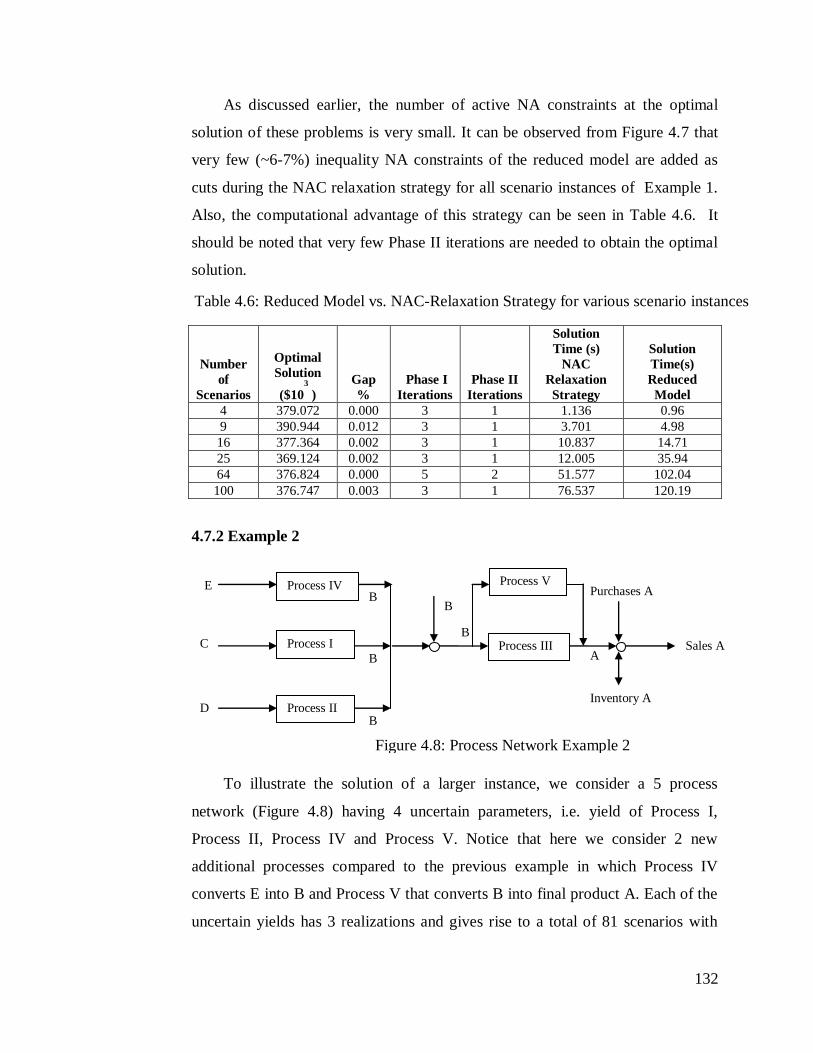
132

As discussed earlier, the number of active NA constraints at the optimal

solution of these problems is very small. It can be observed from Figure 4.7 that

very few (~6-7%) inequality NA constraints of the reduced model are added as

cuts during the NAC relaxation strategy for all scenario instances of Example 1.

Also, the computational advantage of this strategy can be seen in Table 4.6. It

should be noted that very few Phase II iterations are needed to obtain the optimal

solution.

4.7.2 Example 2

To illustrate the solution of a larger instance, we consider a 5 process

network (Figure 4.8) having 4 uncertain parameters, i.e. yield of Process I,

Process II, Process IV and Process V. Notice that here we consider 2 new

additional processes compared to the previous example in which Process IV

converts E into B and Process V that converts B into final product A. Each of the

uncertain yields has 3 realizations and gives rise to a total of 81 scenarios with

Number

of

Scenarios

Optimal

Solution

($103

) Gap

% Phase I

Iterations Phase II

Iterations

Solution

Time (s)

NAC

Relaxation

Strategy

Solution

Time(s)

Reduced

Model 4 379.072 0.000 3 1 1.136 0.96

9 390.944 0.012 3 1 3.701 4.98

16 377.364 0.002 3 1 10.837 14.71

25 369.124 0.002 3 1 12.005 35.94

64 376.824 0.000 5 2 51.577 102.04

100 376.747 0.003 3 1 76.537 120.19

B

B

B

C Process I

Process II D

Process IV E

A

B

B

Purchases A

Sales A

Inventory A

Process III

Process V

Figure 4.8: Process Network Example 2

Table 4.6: Reduced Model vs. NAC-Relaxation Strategy for various scenario instances

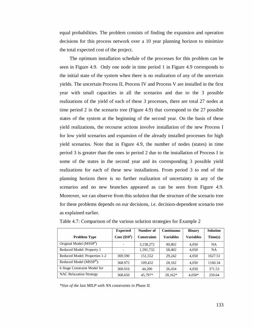
133

equal probabilities. The problem consists of finding the expansion and operation

decisions for this process network over a 10 year planning horizon to minimize

the total expected cost of the project.

The optimum installation schedule of the processes for this problem can be

seen in Figure 4.9. Only one node in time period 1 in Figure 4.9 corresponds to

the initial state of the system when there is no realization of any of the uncertain

yields. The uncertain Process II, Process IV and Process V are installed in the first

year with small capacities in all the scenarios and due to the 3 possible

realizations of the yield of each of these 3 processes, there are total 27 nodes at

time period 2 in the scenario tree (Figure 4.9) that correspond to the 27 possible

states of the system at the beginning of the second year. On the basis of these

yield realizations, the recourse actions involve installation of the new Process I

for low yield scenarios and expansion of the already installed processes for high

yield scenarios. Note that in Figure 4.9, the number of nodes (states) in time

period 3 is greater than the ones in period 2 due to the installation of Process I in

some of the states in the second year and its corresponding 3 possible yield

realizations for each of these new installations. From period 3 to end of the

planning horizon there is no further realization of uncertainty in any of the

scenarios and no new branches appeared as can be seen from Figure 4.9.

Moreover, we can observe from this solution that the structure of the scenario tree

for these problems depends on our decisions, i.e. decision-dependent scenario tree

as explained earlier.

Table 4.7: Comparison of the various solution strategies for Example 2

*Size of the last MILP with NA constraints in Phase II.

Problem Type

Expected

Cost ($103)

Number of

Constraints

Continuous

Variables

Binary

Variables

Solution

Time(s)

Original Model (MSSP0) - 3,158,272 90,802 4,050 NA

Reduced Model: Property 1 - 1,591,732 58,402 4,050 NA

Reduced Model: Properties 1-2 369.590 151,552 29,242 4,050 1627.51

Reduced Model (MSSPR):

Properties 1-3

368.972 109,432 28,162 4,050 1160.34

k-Stage Constraint Model for

k=2

368.916 44,200 26,434 4,050 371.53

NAC Relaxation Strategy 368.650 45,797* 28,162* 4,050* 250.64

134

Figure 4.9: Optimal Solution (Example 2)

The results for this problem are compared in Table 4.7 for the original

(MSSP0), reduced (MSSP

R), k-stage constraint (MSSP

sc) models and NAC

relaxation strategy. The problem was solved within 0.5% optimally tolerance in

all the cases which gives slightly different optimal values. It can be seen that the

problem cannot be solved in the fullspace for the original model and even after

using Property 1, while using the reduced model with Properties 2 and 3, we can

solve it. The solution time for only considering Properties 1-2 is 1.5 times more

than the solution time from considering Properties 1-3, which is expected due to a

factor of around the same order in the number of scenario pairs included in these

models.

The k-stage constraint model was initially solved for two stages (k =2) and it

gives the optimal solution to the problem as there was no realization of any

uncertain parameter after k=2. Because of the inherent property of these

problems, the proposed k-stage constraint model does not need many iterations

and performs better than the reduced model. On the other hand, the NAC

relaxation strategy works well in all the cases because of its generality. As it can

be seen in Table 4.7, the optimal solution obtained from the NAC relaxation

strategy has a slightly lower cost than the other strategies, and it is also

significantly faster than the reduced model and comparable to the k-stage model.

135

The Lagrangean decomposition algorithm was also applied to this 5 process

network problem using the reduced model. The results in Table 4.8 show that

using Lagrangean decomposition algorithm with the reduced model, the problem

can be solved within about 3.5% of optimality gap at the root node after 30

iterations. The solution obtained (UB) at the root node has a higher cost than the

solution obtained from the NAC relaxation strategy ($371,579 vs. $368, 650). On

the other hand, it is faster than the NAC relaxation strategy (181s vs. 251s).

The Lagrangean decomposition strategy has the advantage that if the

problem size is too large to be generated for all the scenarios at once, the model

can be decomposed by scenarios. The k-stage constraint and NAC relaxation

strategies will not work in this case as they need to be solved for all scenarios at

once. It is only in smaller to moderate size problems that the k-stage constraint

strategy and the NAC relaxation strategy may perform better than Lagrangean

decomposition strategy because of the tight lower bounds and corresponding

better solutions obtained in these cases. These trends can be clearly seen from the

two examples considered.

Sub-gradient

Iteration No.

Lower Bound

($103)

Upper Bound

($103)

%

Gap

1* 351.577 371.579 5.383

2* 352.517 371.579 5.130

3* 354.426 371.579 4.616

4* 354.426 371.579 4.616

5* 354.869 371.579 4.497

6* 354.869 371.579 4.497

7* 354.929 371.579 4.481

8* 354.929 371.579 4.481

9 355.235 371.579 4.399

10 355.235 371.579 4.399

30 358.361 371.579 3.557

Time(s) 167.19 13.63 3.557

*problem solved for upper bound generation

Table 4.8: Iterations during Lagrangean Decomposition

algorithm

136

It is also interesting to note that the two-stage stochastic model

corresponding to this example gives about 5% higher total expected cost

($387,421 vs. $368,650) and suggests to invest in all the processes in period 1.

Similar to the Example 1, in the two-stage case the higher cost occurs due to the

absence of appropriate recourse for the investment decisions in the model.

Furthermore, the larger savings compared to the previous example indicate the

advantage of using the multistage stochastic model. Also, note that the total

expected cost is about 3-6 % higher for the expected value problem (EVP) in

comparison to the multistage stochastic programming model for all the cases

considered.

The numerical results presented in this section are very encouraging to solve

multistage stochastic programming problems with endogenous uncertainty using

the proposed solution strategies in reasonable computational time. Although there

are several trade-offs involved in using a particular solution strategy for a

particular class of the problems under uncertainty, the proposed solution strategies

are fairly general and can be applied to many problems classes, specifically to all

the problems that involve endogenous uncertain parameters.

4.8 Conclusions

In this chapter, we have proposed several solution strategies for multistage

stochastic programming problems with endogenous uncertainty. We have

identified a new Property 3 for the models in this class that together with two

properties previously presented by Goel and Grossmann (2006), significantly

reduce the problem size and the solution time. To solve the large instance of these

problems, we have proposed a k-stage constraint strategy that yields the global

optimum in particular cases and is useful for problems where endogenous

uncertainty is revealed during the first few time periods of the planning horizon.

To solve the more general problems of large size, we also proposed a NAC

relaxation strategy based on relaxing the NA constraints and adding them if they

are violated. Finally, we described a Lagrangean Decomposition algorithm that

can predict the rigorous lower bounds for the solution obtained. The proposed

137

solution strategies have been successfully applied to two process network

problems. Moreover, these strategies are applicable to a wide range of problems

having endogenous uncertainty in some of the parameters.

138

Chapter 5

Multistage stochastic programming

approach for offshore oilfield

infrastructure planning under

production sharing agreements and

endogenous uncertainties

5.1 Introduction

In this chapter, we present a general multistage stochastic programming model for

multiperiod investment and operations planning of offshore oil and gas field

infrastructure. The model considers the deterministic models proposed in chapter

2 and 3 as a basis to extend to the stochastic programming using the modeling

framework presented in chapter 4 for endogenous (decision-dependent)

uncertainty problems. In terms of the fiscal contracts, we consider progressive

production sharing agreements, whereas the endogenous uncertainty (type 2) in

the field parameters i.e. field size, oil deliverability, water-oil ratio and gas-oil

ratio is considered, that can only be revealed once an investment is made in the

field and production is started in it. Compared to the conventional models where

either fiscal rules or uncertainty in the field parameters are taken into account, the

proposed model is the first one in the literature that also allows considering both

of these complexities simultaneously. To solve large instances of the problem, the

Lagrangean decomposition approach similar to chapter 4, allowing parallel

139

solution of the scenario subproblems, is implemented in the GAMS grid

computing environment.

The outline of this chapter is as follows. First, in section 5.2 we present a

detailed problem description for offshore oilfield development planning under

production sharing agreements and endogenous uncertainties. The corresponding

multistage stochastic programming model is presented in extensive as well as

compact forms in sections 5.3 and 5.4, respectively. The Lagrangean

decomposition algorithm adapted from chapter 4 is explained in section 5.5 to

solve large instances of the stochastic oilfield planning model. The proposed

model and solution approach are then applied to multiple instances of the two

oilfield development problems in section 5.6 to illustrate their performances.

5.2 Problem statement

Figure 5.1: A typical offshore oilfield infrastructure representation

In this chapter, we consider the development planning of an offshore oil and gas

field infrastructure under complex fiscal rules and endogenous uncertainties. In

particular, a multi-field site, F = {1,2,…}, with potential investments in floating

production storage and offloading (FPSO) facilities, FPSO = {1,2,…} with

Field 1

Field 2

FPSO 2 FPSO 3FPSO 1

Field 3

Field 4Field 5

Ringfence 1

Ringfence 2

Total Oil/Gas

Production

140

continuous capacities and ability to expand them in the future is considered

(Figure 5.1), as in the previous chapters. The connection of a field to an installed

FPSO facility and a number of wells need to be drilled to produce oil from these

fields for the given planning horizon. The planning horizon is discretized into T

time periods, typically each with one year duration. The location of each FPSO

facility and its possible connections to the given fields are assumed to be known.

Notice that each FPSO facility can be connected to more than one field to produce

oil, while a field can only be connected to a single FPSO facility due to

engineering requirements and economic viability of the project. For simplicity, we

only consider FPSO facilities. The proposed model can easily be extended to

other facilities such as tension leg platforms (TLPs). The water produced with the

oil is usually re-injected after separation, while the gas can be sold in the market.

In this case, we consider natural depletion of the reserves, i.e. no water or gas re-

injection. Notice that for convenience to the reader, we included the detailed

problem statement and model in this chapter which contain few common elements

from the previous chapters.

There are three major complexities in the problem considered here:

5.2.1 Nonlinear Reservoir Profiles: We consider three components (oil,

water and gas) explicitly during production from a field. Field deliverability, i.e.

maximum oil flowrate from a field, water-oil-ratio (WOR) and gas-oil-ratio

(GOR) are approximated by cubic equations (a)-(c) (see Figure 5.2), while

cumulative water produced and cumulative gas produced from a field are

represented by fourth order separable polynomials, eqs. (d)-(e), that are derived in

Appendix A. The motivation for using the polynomials for cumulative water

produced and cumulative gas produced in eqs. (d)-(e) as compared to WOR and

GOR in eqs. (b)-(c) is to avoid bilinear terms, eqs. (f)-(g), in the formulation and

allow converting the resulting model into an MILP formulation using piecewise

linear approximations. All the wells in a particular field f are assumed to be

identical for the sake of simplicity leading to the same reservoir profiles, eqs. (a)-

(g), for each of these wells.

141

1,1

2

,1

3

,,1 )()(ˆ dfccfcbfcaQ fffftff

d

f

f (a)

ffffffff dfccfcbfcarow ,2,2

2

,2

3

,2 )()(ˆ

f (b)

ffffffff dfccfcbfcarog ,3,3

2

,3

3

,3 )()(ˆ

f (c)

fffffffff fcdfccfcbfcacw ,4

2

,4

3

,4

4

,4 )()(ˆ

f (d)

fffffffff fcdfccfcbfcacg ,5

2

,5

3

,5

4

,5 )()(ˆ

f (e)

fff xroww .ˆ

f (f)

fff xrogg .ˆ

f (g)

Figure 5.2: Nonlinear Reservoir Characteristics for field (F1) for 2 FPSOs

(FPSO 1 and 2)

0.0

2.0

4.0

6.0

8.0

10.0

12.0

14.0

0.0 0.2 0.4 0.6 0.8 1.0

Oil

del

iver

abil

ity p

er w

ell

(kst

b/d

)

Fractional oil Recovery (fc)

F1-FPSO1

F1-FPSO2

0.0

0.5

1.0

1.5

2.0

2.5

3.0

0.0 0.2 0.4 0.6 0.8 1.0

wat

er-o

il-r

atio

(st

b/s

tb)


F1-FPSO1

F1-FPSO2

0.0

0.2

0.4

0.6

0.8

1.0

1.2

0.0 0.2 0.4 0.6 0.8 1.0

gas

-oil

-rat

io (

ksc

f/st

b)


F1-FPSO1

F1-FPSO2

(a) Oil Deliverability per well for field (F1)

(b) Water to oil ratio for field (F1) (c) Gas to oil ratio for field (F1)

142

5.2.2 Production Sharing Agreements: There are fiscal contracts with the

host government that need to be accounted for during development planning. In

particular, we consider progressive (sliding scale) production sharing agreements

with ringfencing provisions, which are widely used in several countries. The

revenue flow in a typical production sharing agreement (PSA) can be seen as in

Figure 5.3 (World Bank, 2007). First, in most cases, the company pays royalty to

the government at a certain percentage of the total oil produced. After paying the

royalties, some portion of the remaining oil is treated as cost oil by the oil

company to recover its costs. There is a ceiling on the cost oil recovery to ensure

revenues to the government as soon as production starts. The remaining part of

the oil, called profit oil, is divided between oil company and the host government

at a certain percentage. The oil company needs to further pay income tax on its

share of profit oil. Hence, the total contractor’s (oil company) share in the gross

revenue is comprised of cost oil and contractor’s profit oil share after tax.

In this work, we consider a sliding scale profit oil share of the contractor

linked to the cumulative oil produced. For instance, if the cumulative production

(in MMbbl) is in the range of first tier, 2000 txc , the contractor receives 50%

of the profit oil, while if the cumulative production (in MMbbl) reaches in tier 2,

400200 txc , the contractor receives 40% of the profit oil, and so on (see Figure

5.4). Notice that this tier structure is a step function, which requires additional

Income

Tax

Production

Cost Oil Profit Oil

Contractor’s

Share

Government’s

Share

Total Government’s Share Total Contractor’s Share

Contractor’s

after-tax Share

Royalty

Figure 5.3: Revenue flow for a typical Production Sharing Agreement

143

binary variables to model and makes the problem harder to solve. Moreover, the

cost recovery ceiling is considered to be a fraction of the gross revenues in each

time period t. For simplicity, the cost recovery ceiling fraction and income tax

rates are assumed to be a fixed percentages (no sliding scale), and there are no

explicit royalty provisions which is a straightforward extension.

Figure 5.4: Progressive profit oil share of the contractor

A set of ringfences RF = {1,2,…} among the given fields is specified (see

Figure 5.1) to ensure that fiscal calculations are to be done for each ringfence

separately (see chapter 3 for details). For example, the fiscal calculations for

Fields 1-3 (Ringfence 1) and Field 4-5 (Ringfence 2) in Figure 5.1 cannot be

consolidated in one place. These ringfences may or may not have the same fiscal

rules. Qualitatively, a typical ringfencing provision states that the investment and

operational costs for a specified group of fields or block can only be recovered

from the revenue generated from those fields or block. Notice that in general a

field is associated to a single ringfence, while a ringfence can include more than

one field. In contrast, a facility can be connected to multiple fields from different

ringfences for producing oil and gas.

5.2.3 Endogenous Uncertainties:

(a) Uncertain Field Parameters: We consider here the uncertainty in the

field parameters, i.e. field size, oil deliverability per well, water-oil ratio and gas-

oil ratio. These are endogenous uncertain parameters since investment and

operating decisions affect the stochastic process (Jonsbraten et al., 1998; Goel et

al., 2006; Tarhan et al., 2009; and Gupta and Grossmann, 2011a). In particular,

0%

20%

40%

60%

80%

100%

0 200 400 600 800 1000

% P

rofi

t oil

Sh

are

of

Con

trac

tor

Cumulative Oil Production (MMbbl)

144

the uncertainty in the field parameters can only be resolved when an investment is

made in that field and production is started in it. Therefore, optimization decisions

determine the timing of uncertainty realization, i.e. decision-dependent

uncertainty (type 2).

Figure 5.5: Oil deliverability per well for a field under uncertainty

The average profile in Figure 5.5 represents the oil deliverability per well for

a field as a nonlinear polynomial in terms of the fractional oil recovery (eq. (a))

under perfect information. However, due to the uncertainty in the oil

deliverability, the actual profile is assumed to be either the lower or upper side of

the average profile with a given probability. In particular, eq. (h) represents the oil

deliverability per well for a field under uncertainty where parameter oilf , is used

to characterize this uncertainty.

d

foilf

d

f QQ ˆ,

f (h)

For instance, if 1, oilf , then we have a higher oil deliverability than

expected ( 1, oilf ), whereas for 1, oilf a lower than expected oil deliverability

is observed. Since, the uncertain field size (recoverable oil volume, fREC ) is an

0

5

10

15

20

25

0.0 0.1 0.2 0.3 0.4 0.5 0.6 0.7 0.8 0.9 1.0

Qd(k

stb

/d)

Fractional Oil Recovery(fc)

Average

High

Low

Uncertainty in the field size

Low Fractional

Recovery (high size)

High Fractional

Recovery (low size)

Uncertainty in the

oil deliverability

High

Low

H,L

H,H

L,H

L,L

fRECfc

1

145

inverse function of the fraction oil recovery, a higher field size will correspond to

the low fractional oil recovery, whereas a small field size will correspond to the

higher fractional oil recovery for a given amount of the cumulative oil production.

Similarly, eqs. (i) and (j) correspond to the uncertain field profiles for water-

oil-ratio and gas-oil-ratio that are characterized by the uncertain parameters

worf , and gorf , , respectively. Notice that since the cumulative water produced

(eq. (d)) and the cumulative gas produced (eq. (e)) profiles are used in the model,

instead of water-oil-ratio (eq. (b)) and gas-oil-ratio (eq. (c)), the uncertainty in the

parameters worf , and gorf , can be transformed into the corresponding

uncertainty in the parameters wcf , and gcf , as in eqs. (k) and (l), respectively.

In particular, we use the correspondence among the coefficients of these two sets

of the polynomials (see Appendix A) for this transformation.

fworff rowwor ˆ,

f (i)

fgorff roggor ˆ,

f (j)

fwcff cwwc ˆ

,

f (k)

fgcff cggc ˆ,

f (l)

Moreover, the uncertain parameters for every field, i.e.

gorfworfoilfff REC ,,, ,,, are considered to have a number of possible

discrete realizations k

f~

with a given probability. Therefore, all the possible

combinations of these realizations yield a set of scenarios supSs where each

scenario has the corresponding probabilitysp .

(b) Correlation among the uncertain parameters: If the uncertain

parameters are considered to be independent, the total number of scenarios in set

supS grows exponentially with the number of uncertain parameters and their

possible realizations, which makes the problem intractable. For instance, if there

are only 2 fields, then 4 uncertain parameters for each field having 2 realizations

will require 256 scenarios. Therefore, it becomes difficult to solve a multi-field

146

site problem with independent uncertainties in the set

gorfworfoilfff REC ,,, ,,, . Since in practice normally uncertainties are

not independent, we can overcome this limitation by considering that there are

correlations among the uncertain parameters for each individual field. In

particular, the uncertain parameters for a field gorfworfoilfff REC ,,, ,,, are

considered to be dependent. Therefore, only a subset of the possible scenarios

supSS is sufficient to represent the uncertainty. For instance, based on the

practical considerations, we can assume that if a field is of lower size than

expected, then the oil deliverability is also lower ( 1, oilf ). Therefore, the

scenarios with a combinations of higher oil deliverability ( 1, oilf ) and lower

field size are not included in the reduced scenario set and vice-versa. Similarly,

correlations for the water-oil ratio and gas-oil ratio can be considered to

substantially reduce the original scenario set supS . Therefore, the problem can be

considered as selecting a sample of the scenarios for each field, where a scenario

for that field will be equivalent to the selected combinations of the realizations of

the uncertain parameters gorfworfoilfff REC ,,, ,,, .

In the computational experiments, we only consider the extreme cases of the

scenarios assuming perfect correlations, i.e. all uncertain parameters for a field

have either low, medium or high realizations. Note that these assumptions on

correlation among the field parameters are flexible and can be modified

depending on the problem at hand. In addition to the correlation among the

uncertain parameters for each individual field, one can also take into account the

correlation among the fields based on the available information for a particular

oilfield development site to further reduce the total number of scenarios. Notice

also that the model and solution method presented in the chapter is irrespective of

whether a reduced scenario set S is considered or the complete one (supS ).

(c) Uncertainty Resolution Rules: Instead of assuming that the

uncertainties are resolved as soon as a well is drilled in the field, i.e. immediate

resolution, we assume that several wells need to be drilled and production has to

147

be started from the field for this purpose. Moreover, since the uncertain

parameters for a field gorfworfoilfff REC ,,, ,,, are assumed to be

correlated as described above, the timing of uncertainty resolution in these

parameters is also considered to the same. This allows solving much larger multi-

field site instances without losing much in terms of the quality of the solution.

In contrast, Tarhan et al. (2009) considered a single field at a detailed level

where no correlations among the uncertain parameters of the field were

considered, and these parameters were allowed to be revealed independently at

different time periods in the planning horizon. However, the resulting scenario

tree even for a single field became very complex to model and solve. Therefore,

we assume that the uncertainty in all the field parameters

gorfworfoilfff REC ,,, ,,, is resolved if at-least N1 number of wells have

been drilled in the field, and production has been performed from that field for a

duration of at-least N2 years. Notice that these assumptions on uncertainty

resolution rules are flexible and can be adapted depending on the field

information that is available. Moreover, the model can also be extended to the

case where each parameter for a field is allowed to be revealed in different years

based on the work of Tarhan et al. (2009) that will result in a significant increase

in the computation expense.

(d) Decision-dependent scenario trees: The multiperiod planning horizon

and the discrete set of the selected scenarios for each field with given probabilities

can be represented by scenario trees. However, since the timing of the uncertainty

realization for a field (or its corresponding scenarios) depends on the drilling and

operating decisions, the resulting scenario tree is also decision-dependent as was

seen in chapter 4. For instance, if we consider a set of two uncertain fields

2,1F and the selected scenario set based on the parameter correlations for

each field has 2 elements, }~

,~

{ 21

ff , with equal probability. Therefore, the problem

involves the following 4 scenarios each with a probability of 0.25:

)}~

,~

(:4);~

,~

(:3);~

,~

(:2);~

,~

(:1{ 2

2

2

1

1

2

2

1

2

2

1

1

1

2

1

1 S

148

Notice that each of these elements, }~

,~

{ 21

ff , is equivalent to a selected

combination of the realization of the corresponding uncertain parameters, for

example },,,{~ 1

,

1

,

1

,

11

gorfworfoilfff REC . Figure 5.6 represents the scenario tree

for this problem, where the uncertainty in the first field is resolved at the end of

first year, since we drill N1 wells in the field at the beginning of year 1 and

produce from this field during that year (N2 =1). The system can be in two

different states in year 2 depending on the realized value of the uncertain

parameterk

1

~ . Similarly, uncertainty in the field 2 is resolved in year 4 under the

scenarios 3 and 4 due to drilling and operating decisions, whereas it remains

uncertain in the scenarios 1 and 2. Therefore, the resulting scenario tree depends

on the optimization decisions, which are not known a priori, requiring modeling a

superstructure of the all possible scenario trees that can occur based on our

decisions. Notice that the scenario-tree also allows considering the cases where

the number of wells drilled in a field is less than the one required for the

uncertainty resolution (i.e. N1 wells), and therefore, the corresponding scenarios

remain indistinguishable.

Figure 5.6: Decision-dependent scenario tree for two fields

An alternate representation of the decision-dependent scenario-tree (chapter

4) is used to model the problem as a multistage stochastic program in which the

Drill N1 wells in field 1 Year 1

Year 2

Year 5

Year 3

Year 4

1

1

~ 2

1

~

1

2

~ 2

2

~

Drill N1 wells in field 2

1,2 3 4

149

scenarios are treated independently and related through the non-anticipativity

constraints for states of different scenarios that are identical (see Goel and

Grossmann, 2006; and Gupta and Grossmann, 2011a).

The problem is to determine the optimal investment and operating decisions

to maximize the contractor’s expected NPV for a given planning horizon

considering the above production sharing agreements and endogenous

uncertainties. In particular, investment decisions in each time period t and

scenario s include FPSO facilities installation or expansion, and their respective

installation or expansion capacities for oil, liquid and gas, fields-FPSO

connections, and the number of wells that need to be drilled in each field f given

the restrictions on the total number of wells that can be drilled in each time period

t over all the given fields. Operating decisions include the oil/gas production rates

from each field f in each time period t under every scenario s.

It is assumed that the installation and expansion decisions occur at the

beginning of each time period t, while operations take place throughout the time

period. There is a lead time of l1 years for each FPSO facility initial installation,

and a lead time of l2 years for the expansion of an earlier installed FPSO facility.

Once installed, we assume that the oil, liquid (oil and water) and gas capacities of

a FPSO facility can only be expanded once. These assumptions are made for the

sake of simplicity, and both the model and the solution approaches are flexible

enough to incorporate more complexities. In the next section, we propose a

multistage stochastic programming model for oilfield development planning with

production sharing agreements and decision-dependent uncertainty in the field

parameters as described.

5.3 Multistage Stochastic Programming Model

In this section, we present a general multistage stochastic programming model for

offshore oilfield development planning. The proposed model considers the trade-

offs involved between investment and operating decisions, uncertainties in the

field parameters and profit share with the government while maximizing the

overall expected NPV for the contractor. Notice that the model is intended to be

150

solved every year in a rolling horizon manner with updated information, not just

once for the entire planning horizon. The constraints involved in the model are as

follows:

(i) Objective Function: The objective function is to maximize the total expected

NPV of the contractor as in (5.1), which is the summation of the NPVs over all

the scenarios having probabilitiessp . The NPV of a particular scenario s is the

difference between discounted total contractor’s gross revenue share and total cost

over the planning horizon (5.2). The total contractor’s share in a particular time

period t and scenario s is the sum of the contractor’s share over all the ring-fences

(rf) as given in equation (5.3). Similarly, constraints (5.4) and (5.5) represent the

total capital and operating expenses for each scenario s in time period t.

ENPVMax (5.1)

t

stot

t

stot

t

stot

tt

s

s OPERCAPTotalConShdispENPV )( ,,,

(5.2)

rf

s

trf

stot

t TotalConShTotalConSh ,

,

st, (5.3)

rf

s

trf

stot

t CAPCAP ,

,

st, (5.4)

rf

s

trf

stot

t OPEROPER ,

,

st,

(5.5)

(ii) Cost Calculations: The total capital expenses in scenario s for a ring-fence rf

contains two components as given in equation (5.6). One is field specific (eq. 5.7)

that accounts for the connection costs between a field and a FPSO facility, and

cost of drilling the wells for each of the field in that ring-fence rf. The other cost

component is FPSO specific (eq. 5.8) that includes the capital expenses for the

corresponding FPSO facilities. Eq. (5.9) calculates the total cost of an FPSO

facility in time period t for scenario s which is disaggregated in eq. (5.10) over

various fields (and therefore ring-fences as in (5.11)). The cost disaggregation is

done on the basis of the field sizes to which the FPSO is connected (eq. (5.12)-

(5.14)), where set Ffpso is the set of all the fields that can be connected to FPSO

151

facility fpso and the binary variable son

fpsofb ,

, represents the potential connections.

Notice that there is an uncertainty in the recoverable oil volume of the field (

s

fREC ) used in eq. (5.14) that multiplies the binary variable son

fpsofb ,

, . To linearize

the bilinear terms in eq. (5.14), we use exact linearization technique (Glover,

1975) by introducing the positive variables (sfield

tfpsoff

sfield

tfpsoff ZDZD ,

,,,'

,

,,,' 1, ) and

)1,( ,,,,

s

tfpsof

s

tfpsof ZDZD that results in the constraints (5.15)-(5.23).

s

trf

s

trf

s

trf CAPCAPCAP ,,, 21

strf ,, (5.6)

rf r fF fpso F

swell

tf

well

tf

s

tfpsoftfpsof

s

trf IFCbFCCAP ,

,,,,,,,1 strf ,, (5.7)

fpso

s

tfpsorf

s

trf DFPSOCCAP ,,,2

strf ,, (5.8)

)()( ,

,

,

,,

,

,

,

,,

,

,,,

sgas

tfpso

sgas

tfpso

gas

tfpso

sliq

tfpso

sliq

tfpso

liq

tfpso

sFPSO

tfpso

FPSO

tfpso

s

tfpso QEQIVCQEQIVCbFCFPSOC

strf ,, (5.9)

fpsoF

sfield

tfpsof

s

tfpso DFPSOCFPSOC ,

,,,

strf ,, (5.10)

r fF

sfield

tfpsof

s

tfpsorf DFPSOCDFPSOC ,

,,,,

stfpsorf ,,, (5.11)

t

s

tfpsof

son

fpsof bb ,,

,

,

sfpsof ,, (5.12)

son

fpsof

sfield

tfpsof bMDFPSOC ,

,

,

,,

stfpsof ,,, (5.13)

s

tfpso

Ff

s

f

son

fpsof

s

f

son

fpsofsfield

tfpsof FPSOCRECb

RECbDFPSOC

fpso

,

'

'

,

',

,

,,

,,

stfpsof ,,,

(5.14)

s

f

s

tfpsof

s

f

Ff

sfield

tfpsoff RECZDRECZDfpso

,,'

'

,

,,',

stfpsof ,,, (5.15)

sfield

tfpsof

sfield

tfpsoff

sfield

tfpsoff DFPSOCZDZD ,

,,

,

,,',

,

,,', 1

sFftfpsof fpso ,',,, (5.16)

152

son

fpsof

sfield

tfpsoff bUZD ,

,'

,

,,,'

sFftfpsof fpso ,',,,

(5.17)

)1(1 ,

,'

,

,,,'

son

fpsof

sfield

tfpsoff bUZD


01,0 ,

,,,'

,

,,,' sfield

tfpsoff

sfield

tfpsoff ZDZD


s

tfpso

s

tfpsof

s

tfpsof FPSOCZDZD ,,,,, 1

stfpsof ,,, (5.20)

son

fpsof

s

tfpsof bUZD ,

,,,

stfpsof ,,, (5.21)

)1(1 ,

,,,

son

fpsof

s

tfpsof bUZD

stfpsof ,,, (5.22)

01,0 ,,,, s

tfpsof

s

tfpsof ZDZD

stfpsof ,,, (5.23)

The total operating expenses for scenario s in time period t for ring-fence rf ,

eq. (5.24), are the operation costs corresponding to the total amount of liquid and

gas produced.

stot

trf

gas

trf

stot

trf

stot

trf

liq

trft

s

trf gOCwxOCOPER ,

,,

,

,

,

,,, )(

strf ,, (5.24)

(iii) Total Contractor Share Calculations: The total contractor share in scenario

s for ring-fence rf in time period t, eq. (5.25), is the sum of contractor’s after-tax

profit oil share for that ring-fence and the cost oil that it keeps to recover the

expenses. The contractor’s profit oil share after tax in scenario s is the difference

of the contractor’s profit oil share before tax and income tax paid as in constraint

(5.26). The tax paid by the contractor on its profit oil share depends on the given

tax rate (tax

trff , ) as in constraint (5.27).

s

trf

saftertax

trf

s

trf COConShTotalConSh ,

,

,,

strf ,,

(5.25)

s

trf

sbeforetax

trf

saftertax

trf TaxConShConSh ,

,

,

,

,

strf ,,

(5.26)

153

sbeforetax

trf

tax

trf

s

trf ConShfTax ,

,,,

strf ,,

(5.27)

The contractor’s share before tax for scenario s in each time period t is some

fraction of the total profit oil during that period t for ring-fence rf. Note that we

assume here that this profit oil fraction,po

irff , , is based on a decreasing sliding scale

system that is linked to the cumulative amount of oil produceds

trfxc , , where i is

the index of the corresponding tier. Therefore, for possible levels i (i.e. tiers) of

cumulative amount of oil produced by the end of time period t in scenario s, the

corresponding contractor’s profit oil share can be calculated using disjunction

(5.28) where the boolean variable tirfZ ,, is true if the cumulative oil produced lies

between the tier i threshold. This disjunction (5.28) can further be rewritten as

integer and mixed-integer linear constraints (5.29)-(5.36) using the convex-hull

formulation (Raman and Grossmann, 1994).

oil

irf

s

trf

oil

irf

s

trf

PO

irf

sbeforetax

trf

s

tirf

i

UxcL

POfConSh

Z

,,,

,,

,

,

,,

strf ,, (5.28)

i

sbeforetax

tirf

sbeforetax

trf DConShConSh ,

,,

,

,

strf ,, (5.29)

i

s

tirf

s

trf DPOPO ,,,

strf ,, (5.30)

i

s

tirf

s

trf Dxcxc ,,,

strf ,, (5.31)

s

tirf

po

irf

sbeforetax

tirf DPOfDConSh ,,,

,

,,

stirf ,,,

(5.32)

s

tirf

sbeforetax

tirf ZMDConSh ,,

,

,,0

stirf ,,,

(5.33)

s

tirf

s

tirf ZMDPO ,,,,0

stirf ,,,

(5.34)

s

tirf

oil

irf

s

tirf

s

tirf

oil

irf ZUDxcZL ,,,,,,,,

stirf ,,, (5.35)

154

1,, i

s

tirfZ

strf ,,

(5.36)

}1,0{,, s

tirfZ

The cumulative amount of oil produced from a ring-fence rf by the end of

time period t in scenario s is calculated as the sum of the cumulative amount of oil

produced by that time period from all the fields associated to that ring-fence, eq.

(5.37). Constraint (5.38) represents the total profit oil in time period t for a ring-

fence rf as the difference between gross revenue and the cost oil for scenario s.

The gross revenues (5.39) in each time period t for a ring-fence rf in scenario s,

are computed based on the total amount of oil produced and its selling price,

where total oil flow rate in a time period t for ring-fence rf, is calculated as the

sum of the oil production rates over all the fields in that ring-fence, i.e. set Frf , in

equation (5.40). For simplicity, we only consider the revenue generated from the

oil sales, which is much larger in general as compared to the revenue from gas.

rfF

sfield

tf

s

trf xcxc ,

,,

strf ,, (5.37)

s

trf

s

trf

s

trf COREVPO ,,,

strf ,,

(5.38)

stot

trftt

s

trf xREV ,

,,

strf ,, (5.39)

r fF

s

tf

stot

trf xx ,

,

,

strf ,, (5.40)

The cost oil in time period t for a ring-fence rf, constraint (5.41), is

calculated as the minimum of the cost recovery in that time period and maximum

allowable cost oil (cost recovery ceiling) in scenario s. Eq. (5.41) can further be

rewritten as mixed-integer linear constraints (5.42)-(5.47). Cost recovery in time

period t for a ring-fence rf in scenario s, constraint (5.48), is the sum of capital

and operating costs in that period t and cost recovery carried forward from

previous time period t-1. Any unrecovered cost (that is carried forward to the next

period) in time period t for a ring-fence rf, is calculated as the difference between

the cost recovery and cost oil in time period t for a scenario s (eq. (5.49)).

155

),min( ,,,,

s

trf

CR

trf

s

trf

s

trf REVfCRCO

strf ,,

(5.41)

)1( ,

,,,

sco

trf

s

trf

s

trf bMCRCO

strf ,,

(5.42)

)1( ,

,,,

sco

trf

s

trf

s

trf bMCRCO

strf ,,

(5.43)

sco

trf

s

trf

CR

trf

s

trf bMREVfCO ,

,,,,

strf ,,

(5.44)

sco

trf

s

trf

CR

trf

s

trf bMREVfCO ,

,,,,

strf ,,

(5.45)

s

trf

s

trf CRCO ,, strf ,,

(5.46)

s

trf

CR

trf

s

trf REVfCO ,,, strf ,,

(5.47)

s

trf

s

trf

s

trf

s

trf CRFOPERCAPCR 1,,,,

strf ,,

(5.48)

s

trf

s

trf

s

trf COCRCRF ,,,

strf ,,

(5.49)

(iv) Tightening Constraints: The logic constraints (5.50) and (5.51) that

defines the tier sequencing are included in the model to tighten its relaxation.

These constraints can be expressed as integer linear inequalities, (5.52) and

(5.53), respectively, (Raman and Grossmann, 1991). In addition, the valid

inequalities (5.54), are also included that bounds the cumulative contractor’s share

in the cumulative profit oil by the end of time period t based on the sliding scale

profit oil share and cost oil that has been recovered (see chapter 3 for details).

s

irf

T

t

s

tirf ZZ

,',,,

stiiirf ,,',,

(5.50)

s

irf

ts

tirf ZZ

,',1

,,

stiiirf ,,',,

(5.51)

1,',,, s

irf

s

tirf ZZ sTttiiirf ,,,',,

(5.52)

1,',,, s

irf

s

tirf ZZ sttiiirf ,1,,',,

(5.53)

156

)/()()()/( ,,

'

1'

',,1',',

,

,

t

s

rf

PO

irf

ii

i

irf

s

trf

PO

irf

PO

irf

t

sbeforetax


stirf ,,, (5.54)

(v) Reservoir Constraints: Constraints (5.55)-(5.58) predict the reservoir

behavior for each field f in each time period t for a scenario s. In particular,

constraint (5.55) restricts the oil flow rate from each well for a particular FPSO-

field connection in time period t to be less than the deliverability of that field per

well in scenario s. Equation (5.56) represents the field deliverability per well in

scenario s at the beginning of time period t+1 for a particular FPSO-field

connection as the cubic equation in terms of the fractional oil recovered by the

end of time period t from that field. In particular, (5.56a) corresponds to the oil

deliverability in time period 1, while (5.56b) corresponds to the rest of the time

periods in the planning horizon. Notice that the uncertainty in the oil

deliverability profile is characterized by the uncertain parameter s

oil . Constraints

(5.57) and (5.58) represent the separable polynomials for the cumulative water

and cumulative gas produced by the end of time period t for a specific field-FPSO

connection in scenario s, where s

wc and s

gc are the respective uncertain

parameters. The motivation for using polynomials for cumulative water produced

and cumulative gas produced as compared to WOR and GOR is to avoid bilinear

terms in the formulation, and allow converting the resulting MINLP model into an

MILP formulation as explained in the chapter 2.

swelld

tfpsof

swell

tfpsof Qx ,,

,,

,

,,

stfpsof ,,, (5.55)

fpsof

s

oil

swelld

fpsof dQ ,,1

,,

1,,

sfpsof ,, (5.56a)

])()([ ,,1,,,1

2

,,,1

3

,,,1

,,

1,, fpsof

s

tffpsof

s

tffpsof

s

tffpsof

s

oil

swelld

tfpsof dfccfcbfcaQ

sTtfpsof ,,,

(5.56b)

])()()([ ,,,2

2

,,,2

3

,,,2

4

,,,2

,

,,

s

tffpsof

s

tffpsof

s

tffpsof

s

tffpsof

s

wc

swc

tfpsof fcdfccfcbfcaQ

stfpsof ,,, (5.57)

157

])()()([ ,,,3

2

,,,3

3

,,,3

4

,,,3

,

,,

s

tffpsof

s

tffpsof

s

tffpsof

s

tffpsof

s

gc

sgc

tfpsof fcdfccfcbfcaQ

stfpsof ,,, (5.58)

Notice that variables swc

tfpsofQ ,

,, and sgc

tfpsofQ ,

,, will be non-zero in equations

(5.57) and (5.58) ifs

tffc , is non-zero even though that particular field-FPSO

connection is not present. Therefore, additional constraints (5.59)-(5.66) need to

be included to equate the actual cumulative water produced (s

tfpsofwc ,, ) and

cumulative gas produced (s

tfpsofgc ,, ) for a field-FPSO connection by the end of

time period t to the corresponding dummy variables swc

tfpsofQ ,

,, and sgc

tfpsofQ ,

,, only if

that field-FPSO connection is present in time period t, else it is zero. Note that the

motivation for using dummy variables (swc

tfpsofQ ,

,, and

sgc

tfpsofQ ,

,, ) for cumulative

water and cumulative gas flows in equations (5.57)-(5.58) followed by big-M

constraints (5.59)-(5.66), instead of using disaggregated variables for the

fractional recovery in equations (5.57)-(5.58) directly, is to avoid large number of

SOS1 variables while MILP reformulation of this model, as explained in chapter

2.

t

s

fpsof

swc

fpsof

swc

tfpsof

s

tfpsof bMQwc1

,,

,

,

,

,,,, )1(

stfpsof ,,, (5.59)

t

s

fpsof

swc

fpsof

swc

tfpsof

s

tfpsof bMQwc1

,,

,

,

,

,,,, )1(

stfpsof ,,, (5.60)

t

s

fpsof

swc

fpsof

s

tfpsof bMwc1

,,

,

,,,

stfpsof ,,, (5.61)

t

s

fpsof

swc

fpsof

s

tfpsof bMwc1

,,

,

,,,

stfpsof ,,, (5.62)

t

s

fpsof

sgc

fpsof

sgc

tfpsof

s

tfpsof bMQgc1

,,

,

,

,

,,,, )1(

stfpsof ,,, (5.63)

t

s

fpsof

sgc

fpsof

sgc

tfpsof

s

tfpsof bMQgc1

,,

,

,

,

,,,, )1(

stfpsof ,,, (5.64)

158

t

s

fpsof

sgc

fpsof

s

tfpsof bMgc1

,,

,

,,,

stfpsof ,,, (5.65)

t

s

fpsof

sgc

fpsof

s

tfpsof bMgc1

,,

,

,,,

stfpsof ,,, (5.66)

Eq. (5.67) and (5.68) compute the water and gas flow rates in time period t

from a field to FPSO facility in scenario s as the difference of cumulative amounts

produced by the end of current time period t and previous time period t-1 divided

by the time duration of that period.

t

s

tfpsof

s

tfpsof

s

tfpsof wcwcw /)( 1,,,,,,

stfpsof ,,, (5.67)

t

s

tfpsof

s

tfpsof

s

tfpsof gcgcg /)( 1,,,,,,

stfpsof ,,, (5.68)

(vi) Field-FPSO flow constraints: The total oil flow rate in (5.69) from each

field f in time period t for a scenario s is the sum of the oil flow rates that are

directed to FPSO facilities in that time period t, whereas oil that is directed to a

particular FPSO facility from a field f in scenario s is calculated as the

multiplication of the oil flow rate per well and number of wells available for

production in that field (eq. (5.70)). Eq. (5.71) computes the cumulative amount

of oil produced from field f by the end of time period t in scenario s, while (5.72)

represents the fractional oil recovery by the end of time period t. The cumulative

oil produced in scenario s is also restricted in (5.73) by the recoverable amount of

oil from the field. Eqs. (5.74)-(5.76) compute the total oil, water and gas flow

rates into each FPSO facility, respectively, in time period t from all the given

fields in each scenario s. The total oil, water and gas flowrates in each time period

t for scenario s are calculated as the sum of the production rate of these

components over all the FPSO facilities in equations (5.77)-(5.79), respectively.

fpso

s

tfpsof

s

tf xx ,,,

stf ,, (5.69)

swell

tfpsof

swell

tf

s

tfpsof xNx ,

,,

,

,,,

stfpsof ,,, (5.70)

159

)(1

,,

t

s

f

s

tf xxc

stf ,, (5.71)

s

f

s

tfs

tfREC

xcfc

,

,

stf ,, (5.72)

s

f

s

tf RECxc , stf ,,

(5.73)

f

s

tfpsof

s

tfpso xx ,,,

stfpso ,, (5.74)

f

s

tfpsof

s

tfpso ww ,,,

stfpso ,, (5.75)

f

s

tfpsof

s

tfpso gg ,,,

stfpso ,, (5.76)

fpso

s

tfpso

stot

t xx ,

,

st, (5.77)

fpso

s

tfpso

stot

t ww ,

,

st, (5.78)

fpso

s

tfpso

stot

t gg ,

,

st, (5.79)

(vii) FPSO Capacity Constraints: Eqs. (5.80)-(5.82) restrict the total oil, liquid

and gas flow rates into each FPSO facility to be less than its corresponding

capacity in each time period t, respectively. These three different kinds of

capacities of a FPSO facility in time period t are computed by equalities (5.83)-

(5.85) as the sum of the corresponding capacity at the end of previous time period

t-1, installation capacity at the beginning of time period t-l1 and expansion

capacity at the beginning of time period t-l2, where l1 and l2 are the lead times for

FPSO installation and expansions, respectively.

160

soil

tfpso

s

tfpso Qx ,

,, stfpso ,,

(5.80)

sliq

tfpso

s

tfpso

s

tfpso Qwx ,

,,,

stfpso ,, (5.81)

sgas

tfpso

s

tfpso Qg ,

,, stfpso ,,

(5.82)

soil

ltfpso

soil

ltfpso

soil

tfpso

soil

tfpso QEQIQQ ,

,

,

,

,

1,

,

, 21

stfpso ,, (5.83)

sliq

ltfpso

sliq

ltfpso

sliq

tfpso

sliq

tfpso QEQIQQ ,

,

,

,

,

1,

,

, 21

stfpso ,, (5.84)

sgas

ltfpso

sgas

ltfpso

sgas

tfpso

sgas

tfpso QEQIQQ ,

,

,

,

,

1,

,

, 21

stfpso ,, (5.85)

(viii) Logic Constraints: Inequalities (5.86) and (5.87) restrict the installation

and expansion of a FPSO facility to take place only once, respectively, while

inequality (5.88) states that the connection between a FPSO facility and a field

can be installed only once during the whole planning horizon. Inequality (5.89)

ensures that a field can be connected to at most one FPSO facility in each time

period t, while (5.90) states that at most one FPSO-field connection is possible for

a field f during the entire planning horizon under each scenario s. Constraints

(5.91) and (5.92) state that the expansion in the capacity of a FPSO facility and

the connection between a field and a FPSO facility, respectively, in time period t

can occur only if that FPSO facility has already been installed by that time period.

1, Tt

s

tfpsob

sfpso, (5.86)

1,

, Tt

sex

tfpsob

sfpso, (5.87)

1,

,, Tt

sc

tfpsofb

sfpsof ,, (5.88)

1,

,, fpso

sc

tfpsofb

stf ,, (5.89)

1,

,, Tt fpso

sc

tfpsofb

sf ,

(5.90)

161

t

s

fpso

sex

tfpso bb1

,

,

,

stfpso ,, (5.91)

t

s

fpso

sc

tfpsof bb1

,

,

,,

stfpsof ,,, (5.92)

(ix) Upper bounding constraints: Inequality (5.93) states that the oil flow rate

per well from a field f to a FPSO facility in time period t will be zero if that

FPSO-field connection is not available in that time period in a scenario s.

Constraints (5.94)-(5.99) are the upper-bounding constraints on the installation

and expansion capacities for FPSO facilities in time period t for each scenario s.

The additional upper bounds on the oil, liquid and gas expansion capacities of

FPSO facilities, (5.100)-(5.102), come from the fact that these expansion

capacities should be less than a certain fraction (µ) of the initial built capacities,

respectively.

t

sc

fpsof

oilwell

fpsof

swell

tfpsof bUx1

,

,,

,

,

,

,,

stfpsof ,,, (5.93)

s

tfpso

oil

fpso

soil

tfpso bUQI ,

,

, stfpso ,,

(5.94)

s

tfpso

liq

fpso

sliq

tfpso bUQI ,

,

, stfpso ,,

(5.95)

s

tfpso

gas

fpso

sgas

tfpso bUQI ,

,

, stfpso ,,

(5.96)

sex

tfpso

oil

fpso

soil

tfpso bUQE ,

,

,

, stfpso ,,

(5.97)

sex

tfpso

liq

fpso

sliq

tfpso bUQE ,

,

,

, stfpso ,,

(5.98)

sex

tfpso

gas

fpso

sgas

tfpso bUQE ,

,

,

, stfpso ,,

(5.99)

soil

tfpso

soil

tfpso QQE ,

1,

,

,

stfpso ,, (5.100)

sliq

tfpso

sliq

tfpso QQE ,

1,

,

,

stfpso ,, (5.101)

sgas

tfpso

sgas

tfpso QQE ,

1,

,

,

stfpso ,, (5.102)

(x) Well drilling limitations: The number of wells available for production from

a field in scenario s is calculated from (5.103) as the sum of the wells available at

the end of previous time period and the number of wells drilled at the beginning

162

of time period t. The maximum number of wells that can be drilled over all the

fields during each time period t and in each field f during complete planning

horizon are restricted by the respective upper bounds in (5.104) and (5.105).

swell

tf

swell

tf

swell

tf INN ,

,

,

1,

,

, stf ,, (5.103)

well

t

f

swell

tf UII ,

,

st,

(5.104)

well

f

swell

tf UNN ,

, stf ,, (5.105)

(xi) Initial Non-anticipativity Constraints: In addition to the above constraints

(5.1)-(5.105) that are equivalent to the constraints for the deterministic model

with fiscal rules for each scenario s as in chapter 3, we need the initial non-

anticipativity constraints, eqs. (5.106)-(5.115), for time periods TTI where the

set IT may include only first or few initial time periods. These constraints ensure

that we make the same decisions (FPSO installations, expansions and their oil,

liquid, gas capacities; well drilling schedule and field-FPSO connections) in

scenarios s and s’ until uncertainty in the any of the parameters cannot be

revealed.

I

sFPSO

tfpso

sFPSO

tfpso Ttssfpsobb ,',,',

,

,

,

(5.106)

I

sex

tfpso

sex

tfpso Ttssfpsobb ,',,',

,

,

,

(5.107)

I

s

tfpsof

s

tfpsof Ttssfpsofbb ,',,,'

,,,,

(5.108)

I

swell

tf

swell

tf TtssfII ,',,',

,

,

,

(5.109)

I

soil

tfpso

soil

tfpso TtssfpsoQIQI ,',,',

,

,

,

(5.110)

I

sliq

tfpso

sliq


,

,

,

(5.111)

I

sgas

tfpso

sgas


,

,

,

(5.112)

I

soil

tfpso

soil

tfpso TtssfpsoQEQE ,',,',

,

,

,

(5.113)

I

sliq

tfpso

sliq


,

,

,

(5.114)

I

sgas

tfpso

sgas


,

,

,

(5.115)

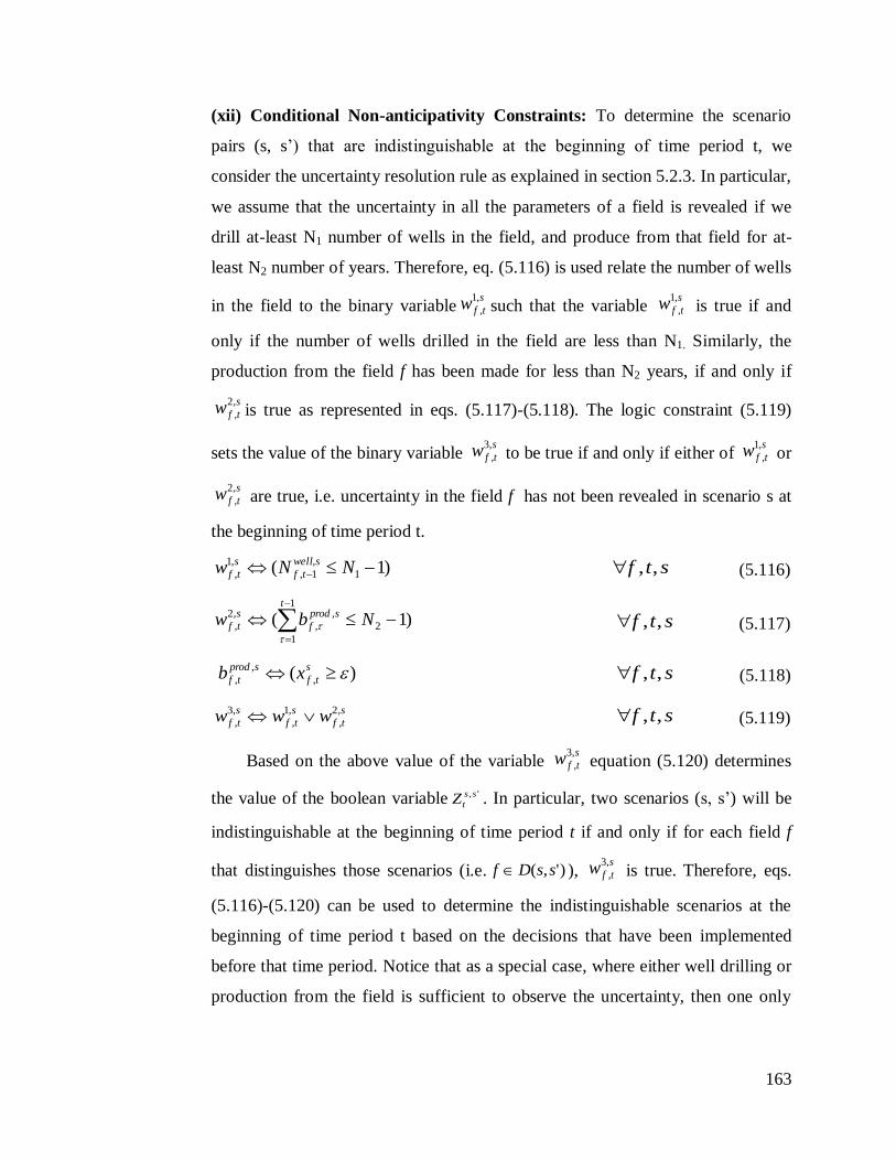
163

(xii) Conditional Non-anticipativity Constraints: To determine the scenario

pairs (s, s’) that are indistinguishable at the beginning of time period t, we

consider the uncertainty resolution rule as explained in section 5.2.3. In particular,

we assume that the uncertainty in all the parameters of a field is revealed if we

drill at-least N1 number of wells in the field, and produce from that field for at-

least N2 number of years. Therefore, eq. (5.116) is used relate the number of wells

in the field to the binary variables

tfw ,1

, such that the variable s

tfw ,1

, is true if and

only if the number of wells drilled in the field are less than N1. Similarly, the

production from the field f has been made for less than N2 years, if and only if

s

tfw ,2

, is true as represented in eqs. (5.117)-(5.118). The logic constraint (5.119)

sets the value of the binary variable s

tfw ,3

, to be true if and only if either of s

tfw ,1

, or

s

tfw ,2

, are true, i.e. uncertainty in the field f has not been revealed in scenario s at

the beginning of time period t.

)1( 1

,

1,

,1

, NNw swell

tf

s

tf stf ,, (5.116)

)1( 2

1

1

,

,

,2

,

Nbwt

sprod

f

s

tf

stf ,, (5.117)

)( ,

,

, s

tf

sprod

tf xb

stf ,,

(5.118)

s

tf

s

tf

s

tf www ,2

,

,1

,

,3

,

stf ,,

(5.119)

Based on the above value of the variable s

tfw ,3

, equation (5.120) determines

the value of the boolean variable ',ss

tZ . In particular, two scenarios (s, s’) will be

indistinguishable at the beginning of time period t if and only if for each field f

that distinguishes those scenarios (i.e. )',( ssDf ), s

tfw ,3

, is true. Therefore, eqs.

(5.116)-(5.120) can be used to determine the indistinguishable scenarios at the

beginning of time period t based on the decisions that have been implemented

before that time period. Notice that as a special case, where either well drilling or

production from the field is sufficient to observe the uncertainty, then one only

164

needs to consider eq. (5.116) or eqs. (5.117)-(5.118), respectively, and eq. (5.120)

without introducing the additional variable s

tfw ,3

, .

s

tfssDf

ss

t wZ ,3

,)',(

',

tss ,',

(5.120)

The conditional non-anticipativity constraints in disjunction (5.121) equate

the decisions in scenarios s and s’ for the later time periods TTC , if these

scenarios are indistinguishable at the beginning of time period t, i.e. for which

',ss

tZ is true calculated in eq. (5.120).

C

ss

t

sgas

tfpso

sgas

tfpso

sliq

tfpso

sliq

tfpso

soil

tfpso

soil

tfpso

sgas

tfpso

sgas

tfpso

sliq

tfpso

sliq

tfpso

soil

tfpso

soil

tfpso

swell

tf

swell

tf

s

tfpsof

s

tfpsof

sex

tfpso

sex

tfpso

sFPSO

tfpso

sFPSO

tfpso

ss

t

TtssZ

fpsoQEQE

fpsoQEQE

fpsoQEQE

fpsoQIQI

fpsoQIQI

fpsoQIQI

fII

fpsofbb

fpsobb

fpsobb

Z

,',

,

'.

',

,

,

,

',

,

,

,

',

,

,

,

',

,

,

,

',

,

,

,

',

,

,

,

',

,

,

,

'

,,,,

',

,

,

,

',

,

,

,

',

(5.121)

The multistage stochastic mixed-integer nonlinear disjunctive programming

model (MSSP-ND) for offshore oilfield investment and operations planning

involves constraints (5.1)-(5.13), (5.15)-(5.27), (5.29)-(5.40), (5.42)-(5.49),

(5.52)-(5.121) that consider endogenous uncertainty in the field parameters and

sliding scale production sharing agreements with ringfencing provisions. In

particular, constraints (5.56b)- (5.58) and (5.70) are nonlinear and non-convex

constraints in the model. These constraints can be linearized using exact

165

linearization and piecewise linear approximation techniques described in chapter

2 to convert the nonlinear model (MSSP-ND) to a linear one (MSSP-LD). Notice

that the resulting model will be an extension of the deterministic MILP fiscal

model (Model 3F) in chapter 3 to the stochastic case using the modeling

framework presented in chapter 4.

5.4 Compact representation of the multistage stochastic model

The proposed multistage stochastic mixed-integer linear disjunctive programming

model (MSSP-LD) in the previous section can be represented in the following

compact form:

(MD)

Ss Tt

s

tt

s xcpzmax (5.122)

staxAts s

t

t

ss ,..

(5.123)

SssTtxx I

s

t

s

t ',,' (5.124)

SssTtxxxFZ C

s

t

ssss

t ',,)....,( 121

', (5.125)

SssTtZ

xx

Z

C

ss

t

s

t

s

t

ss

t

',,',

'

',

(5.126)

',, JjstIxs

jt (5.127)

'\,, JJjstRxs

jt (5.128)

The objective function (5.122) in the above model (MD) maximizes the

expectation of an economic criterion over the set of scenarios Ss , and over a set

of time periods Tt , which is equivalent to eq. (5.1). For a particular scenario s,

inequality (5.123) represents constraints that govern decisions s

tx in time period t

and link decisions across time periods. These individual scenario constraints

correspond to the eqs. (5.2)-(5.13), (5.15)-(5.27), (5.29)-(5.40), (5.42)-(5.49) and

(5.52)-(5.105), where the nonlinear and non-convex constraints (5.56b)- (5.58)

166

and (5.70) have been linearized using exact linearization and piecewise linear

approximation techniques described in chapter 2.

Non-anticipativity (NA) constraints for initial time periods TTI are given

by equations (5.124) for each scenario pair (s,s’) to ensure the same decisions in

all the scenarios, which are the compact representation for constraints (5.106)-

(5.115). The conditional NA constraints are written for the later time periods

TTC in terms of logic propositions (5.125) and disjunctions (5.126). Notice

that the set of initial time periods IT may include first few years of the planning

horizon until uncertainty cannot be revealed, while CT represents the rest of the

time periods in the planning horizon. The function )....,( 121

s

t

ss xxxF in eq. (5.125)

is an uncertainty resolution rule for a given pair of scenarios s and s’ that

determines the value of the corresponding boolean variable ',ss

tZ based on the

decisions that have been implemented so far as shown in eqs. (5.116)-(5.120). The

variable ',ss

tZ is further used in disjunction (5.126) to ensure the same decisions in

scenarios s and s’ if these are still indistinguishable in time period t, which is

similar to the disjunctions (5.121). Equations (5.127)-(5.128) define the domain of

the discrete and continuous variables in the model.

Notice that the model with a reduced number of scenario pairs (s,s’) that are

sufficient to represent the non-anticipativity constraints can be obtained from

model (MD) after applying the three properties presented in chapter 4. These

properties are defined on the basis of symmetry, adjacency and transitivity

relationship among the scenarios. The reduced model (MDR) can be formulated

from (MD) as follows, where 3P is the set of minimum number of scenario pairs

that are required to represent non-anticipativity in each time period t,

(MDR)

Ss Tt

s

tt

s xcpzmax (5.122)

staxAts s

t

t

ss ,..

(5.123)

3

' )',(, PssTtxx I

s

t

s

t (5.129)

167

3121

', )',(,)....,( PssTtxxxFZ C

s

t

ssss

t (5.130)

3

',

'

',

)',(, PssTtZ

xx

Z

C

ss

t

s

t

s

t

ss

t

(5.131)

',, JjstIxs

jt (5.127)

'\,, JJjstRxs

jt (5.128)

The mixed-integer linear disjunctive model (MDR) can be further converted

to a mixed-integer linear programming model (MLR). First, the logic constraints

(5.130) are re-written as the mixed-integer linear constraints eq. (5.132) based on

the uncertainty resolution rule where ',ss

tz is a binary variable that takes a value of

1 if scenario pair (s,s’) is indistinguishable in time period t, else it is zero. The

disjunction (5.131) can then be converted to mixed-integer linear constraints

(5.133) and (5.134) using the big-M formulation. The resulting mixed-integer

linear model (MLR) includes constraints (5.122), (5.123), (5.129), (5.132),

(5.133), (5.134), (5.127) and (5.128).

3

', )',(, PssTtdzCxB C

s

t

ss

t

s

t

s

t

s

t (5.132)

3

'', )',(,)1( PssTtxxzM C

s

t

s

t

ss

t (5.133)

3


s

t

s

t

ss

t (5.134)

Figure 5.7 represents the block angular structure of model (MLR), where we

can observe that the initial (eq. (5.129)) and conditional (eqs. (5.132), (5.133) and

(5.134)) non-anticipativity constraints link the scenario subproblems. Therefore,

these are the complicating constraints in the model. However, this structure

allows decomposing the fullspace problem into smaller subproblems by relaxing

the linking constraints as in chapter 4. It should be noted that the NACs

(especially conditional NACs) represent a large fraction of the total constraints in

the model. For clarity, we use this compact representation (MLR) in the next

section to describe the solution approach instead of the detailed model (MSSP-

LD) presented in the previous section.

168

Figure 5.7: Structure of a typical Multistage Stochastic Program with Endogenous

uncertainties

5.5 Solution Approach

The reduced model (MLR) is composed of scenario subproblems connected

through the initial (eq. (5.129)) and conditional (eqs. (5.132), (5.133) and (5.134))

non-anticipativity (NA) constraints. If these NA constraints are either relaxed or

dualized using Lagrangean decomposition, then the problem decomposes into

smaller subproblems that can be solved independently for each scenario within an

iterative scheme for the multipliers as described in Carøe and Schultz (1999) and

in Gupta and Grossmann (2011a). In this way, we can effectively decompose and

solve the large-scale oilfield development planning instances. The Lagrangean

decomposition algorithm of Figure 5.8 for MSSP with endogenous uncertainties

as proposed in chapter 4 involves obtaining the upper bound (UB) by solving the

Lagrangean problem (L1-MLR) with fixed multipliers',ss

t . The Lagrangean

problem (L1-MLR) is formulated from the mixed-integer linear reduced model

(MLR) by relaxing all the conditional NA constraints (5.132), (5.133) and

(5.134), and dualizing all the initial NA constraints (5.129) as penalty terms in the

objective function. This gives rise to the subproblems for each scenario Ss ,

(L1-MLRs) that can be solved in parallel.

Scenario Constraints

Initial NACs

Conditional NACs

169

(L1-MLR)

1 3)',(

'', )(maxTt Pss

s

t

s

t

ss

t

Ss Tt

s

tt

s xxxcp (5.135)

staxAts s

t

t

ss ,..

(5.136)

',,}1,0{ Jjstxs

jt (5.137)

'\,, JJjstRxs

jt (5.138)

(L1-MLRs)

1 3 3

')',(

'),'(

,'', )(maxTt

ssPss

ssPss

ss

t

ss

t

s

t

Tt

s

tt

s xxcp (5.139)

taxAts s

t

t

ss

.. (5.140)

',}1,0{ Jjtxs

jt (5.141)

'\, JJjtRxs

jt (5.142)

The lower bound (LB) or feasible solution is generated by using a heuristic

based on the solution of the Lagrangean problem (L1-MLR). In this heuristic, we

fix the decisions obtained from the above problem (L1-MLR) in the reduced



LB = -∞

UB = ∞

Yes

Solve Lagrangean subproblem with fixed multipliers to get UB

Gap < ε

or k > kmax

Stop

Find LB (Feasible Solution)


No




170

problem (MLR) such that there is no violation of NA constraints and solve it to

obtain the lower bound. The sub-gradient method by Fisher (1985) is used during

each iteration to update the Lagrangean multipliers. The algorithm stops when

either a maximum iteration/time limit is reached, or the difference between the

lower and upper bounds, LB and UB, is less than a pre-specified tolerance.

Notice that the extended form of this method relying on duality based branch

and bound search, has also been proposed in Goel and Grossmann (2006), Tarhan

et al. (2009), and Tarhan et al. (2011) to close the gap between the upper and the

lower bounds. Moreover, a new Lagrangean decomposition algorithm is proposed

in the next chapter 6 to further improve the quality of the dual bound at the root

node.

5.6 Numerical results

In this section, we present computational results for the offshore oilfield

development planning examples under endogenous uncertainty in the field

parameters, which resolves as a function of investment and operating decisions as

described before. Moreover, we consider a case where progressive production

sharing agreements are also present. The multistage stochastic MILP model

(MLR) presented in section 5.4 is considered that maximizes the expected NPV

value over the given planning horizon. The model is implemented in GAMS

23.6.3 and run on an Intel Core i7, 4GB RAM machine using CPLEX 12.2 solver

for all the instances.

5.6.1 3 Oilfield Planning Example

Case (i): Uncertainty in the field size only (4 scenarios)

In this instance, we consider 3 oilfields and 3 potential FPSO’s that can be

installed. There are a total of 9 possible connections among field-FPSO (Figure

5.9), and 30 wells can be drilled in the fields over the planning horizon of 10

years. Field 3 has a recoverable oil volume (field size) of 500 MMbbls. However,

there is uncertainty in the size of fields 1 and 2, where each one has two possible

realizations (low, high) with equal probability. Therefore, there are a total of 4

scenarios each with a probability of 0.25 (see Table 5.1). Notice that for

171

simiplicity we only consider the cases with same probabilities for all the scenarios

thoughout this chapter. In our future paper, if it would be possible, we will

include more realistic probability values for the examples.

Figure 5.9: 3 oilfield planning example

Table 5.1: 3 oilfield planning example, case (i)

Scenarios s1 s2 s3 s4

Field 1 Size (MMbbls) 57 403 57 403


Scenario Probability 0.25 0.25 0.25 0.25

It is assumed that the uncertainty in field 1 size is revealed after drilling 3

wells (N1= 3) in the field and producing for 1 year (N2= 1) from it. Whereas, field

2 needs at-least 4 wells to be drilled (N1= 4) and one year of production (N2= 1)

for this purpose. The problem is to determine the optimum investment (FPSO

installations and expansions, field-FPSO connections and well drilling) and

operating decisions (oil production rate) with an objective to maximize the total

expected NPV (ENPV) over the planning horizon.

Table 5.2: Model statistics for the 3 oilfield example, case (i)

FPSO 1 FPSO 3

Field 1

Field 3

Field 2

Total Oil/Gas Production

FPSO 2

Problem Type

Number of

Constraints

Continuous

Variables

Discrete

Variables

SOS1

Variables

Reduced Model (MLR) 16,473 9,717 876 240

Individual Scenario 3,580 2,390 179 60

172

Figure 5.10: Optimal solution for 3 oilfield example, case (i)

The optimal ENPV for the problem is $11.50 x109 when the reduced model

(MLR) is solved in fullspace using CPLEX 12.2 solver requiring 1184s. Table 5.2

presents the model statistics for this instance. The solution suggests installing only

FPSO 3 in the first year (see Figure 5.10) with a capacity of 500 kstb/d and 333.5

MMSCF/d for liquid and gas, respectively. The facility is available to produce at

the beginning of year 4 due to a lead time of three years. Then, we drill 3, 5 and

12 wells in fields 1,2 and 3, respectively, given the drilling-rig limitation of a total

20 wells in a year. Since, fields 1 and 2 have uncertainties, based on the

realization of the uncertainty in their field sizes, more wells are drilled in these

fields in the future for the favorable scenarios compared to the unfavorable

outcomes, whereas no more wells are drilled in field 3. In particular, the favorable

scenarios for field 1 are scenarios 2 and 4, where a total of 7 wells are drilled in

the field. On the other hand, field 2 has favorable scenarios 3 and 4, where a total

of 11 wells are drilled in the field. Due to the different drilling and production

decisions in different scenarios based on the uncertainty realizations, the capacity

L,L H,H

drill (3,5,12)

drill (1,0) (4,0) (0,6) (4,6)

H,L L,HUncertainty

Revealed

Year 1

Year 4

Year 5

Year 6

Year 7

Year 8

Year 9

Year 10

Build FPSO 3 (500, 333.5)

drill (0,2) (0,4) (3,0)

173

of FPSO3 is expanded in year 5 for scenarios 2, 3 and 4, whereas no expansion is

made in the FPSO3 capacity in scenario 1. We can observe that the optimal

scenario-tree is decision-dependent which is not known a-priori (Figure 5.10).

Figure 5.11: Lagrangean decomposition results for 3 oilfield example, case (i)

The multistage stochastic model (MLR) is also solved using the Lagrangean

decomposition algorithm presented in the previous section that relies on dualizing

the initial NACs and removing the conditional NACs. Figure 5.11 demonstrates

the progress of the bounds obtained at the root node using this decomposition

approach. A termination criterion of either 1% gap or 20 sub-gradient iterations is

used. We can observe that the problem can be solved in ~1% optimality tolerance

in only 466s for the sequential implementation compared to the fullspace model

that takes 1184s. Moreover, the parallel implementation of the Lagrangean

decomposition algorithm in GAMS with 8 processors only takes 259s. Therefore,

the proposed strategy reduces the solution time for this 4 scenario instance by

more than 75% compared to the fullspace model. It is also important to note that

the reformulation of the MINLP model (Model 2) to MILP approximation (Model

3) in chapter 2 allows us to use this decomposition strategy with valid upper and

11.45

11.50

11.55

11.60

11.65

11.70

11.75

11.80

11.85

0 2 4 6 8 10 12 14 16 18 20

EN

PV

(bil

lion

doll

ars)

Iterations

LB

UB

174

lower bounds on the objective function value, without solving the non-convex

MINLP model to global optimality which is quite expensive. Notice that the

solution of the expected value problem considering the mean value of the field

sizes is $11.28 x109. Therefore, the value of the stochastic solution for this case is

$220 x106 or ~2%.

Case (ii): Uncertainty in the field size, oil deliverability, WOR and GOR (4

scenarios)

In this case, we consider uncertainty in the field size, oil deliverability, water-oil

ratio (WOR) and gas-oil-ratio (GOR) for oilfields 1 and 2. Notice that oil

deliverability, WOR and GOR are represented by the univariate polynomials in

terms of the fractional oil recovery as shown in equations (5.143)-(5.145),

respectively.

)( fcgQ o

d (5.143)

)( fcgwor w (5.144)

)( fcggor g (5.145)

The uncertainty in oil deliverability, WOR and GOR is characterized by the

uncertainty in corresponding parameters o , w and g . We assume that the

uncertain parameters for a field are correlated, and that uncertainty in these

parameters is resolved at the same time as explained earlier. This allows us to

reduce a large number of scenarios in the problem. The two possible

combinations of these parameters for each field results in a total of 4 scenarios

each with a probability of 0.25 as can be seen in Table 5.3. The data for the rest of

the problem are as in case (i) presented above.

Table 5.4 summarizes the computational results for this case, and we can

observe the similar trends as in the previous case. In particular, the fullspace

multistage stochastic model using CPLEX 12.2 takes >10,000s to solve the

problem to optimality and it yields an expected NPV value of $11.95x109. The

sequential and parallel implementations (8 processors) of the proposed

175

Lagrangean decomposition approach provide a solution of $11.94x109 with more

than an order of magnitude reduction in solution times. To further reduce the gap

between the upper and the lower bounds, the algorithm can be extended to the

duality based branch and bound search procedure as proposed in Goel and

Grossmann (2006). In addition, an improved Lagrangean decomposition approach

that yields a tighter dual bound at the root node is also presented in the next

chapter.

Table 5.3: 3 oilfield planning example, case (ii)


Field 1

Size (MMbbls) 57 403 57 403

o 0.75 1.25 0.75 1.25

w 0.75 1.25 0.75 1.25

g 0.75 1.25 0.75 1.25

Field 2

Size (MMbbls) 80 80 560 560

o 0.75 0.75 1.25 1.25

w 0.75 0.75 1.25 1.25

g 0.75 0.75 1.25 1.25


Table 5.4: Computational results for 3 oilfield example, case (ii)

Fullspace Lagrangean Decomposition

Sequential Parallel

UB ($109) 11.95 12.14 12.14

LB ($109) 11.95 11.94 11.94

Solution Time (s) 10390 438 257

% Gap 0% 1.66% 1.66%

Subgradient iterations - 20 20

Case (iii): Uncertainty in the field size and progressive production sharing

agreements

We also extend the 3 oilfield example to the case where we include the

progressive production sharing agreements and a planning horizon of 15 years.

176

Table 5.5 represents the sliding scale profit share of the contactor involving 3 tiers

that are defined on the basis of the cumulative oil production. The cost recovery

ceiling of 50% of the gross revenue every year and an income tax rate of 30% is

also considered. There is uncertainty in the field sizes (field 1 and 2) with a total

of 4 scenarios as described in Table 5.1.

Table 5.5: Sliding scale contractor’s profit oil share for the 3 oilfield example,

case (iii)

Tiers Cumulative Oil Produced Contractor’s Share in Profit

Oil

Tier 1 0-350 MMbbl 50%

Tier 2 350-700 MMbbl 40%

Tier 3 >700 MMbbl 20%

Table 5.6: Computational results for 3 oilfield example, case (iii)

Fullspace Model Lagrangean Decomposition

#

Constraints

#

Dis.

Var.

#

Cont.

Var.

ENPV

($109)

Time

(s)

ENPV

($109)

Sequential

Time (s)

Parallel

Time

(s)

27,113 1,536 15,857 $2.97

(>21%)

>36,000 $3.04

(0.7%)

8,990 4,002

The multistage stochastic model becomes very difficult to solve for this

instance in fullspace due to the complexities introduced in the model by the non-

anticipativity constraints, and the disjunction for representing the sliding scale

fiscal rules. In particular, the best solution obtained after 10 hours in fullspace

using CPLEX 12.2 solver is $2.97x109

with more than 21% of optimality gap (see

Table 5.6). On the other hand, the proposed Lagrangean decomposition can solve

this problem in approximately 2 hrs for the sequential implementation of the

scenario subproblem solutions, and in about 1 hr for the parallel implementation

(8 processors). Both the cases yield a higher ENPV $3.04x109 within a 0.7% of

optimality tolerance. Therefore, this example illustrates the importance of the

177

decomposition algorithm, and its parallel implementation, as more complexities

are added to the problem, such as the progressive fiscal rules.

5.6.2 5 Oilfield Planning Example



This is a larger example for oilfield planning problem under uncertainty than

the previous one, where we consider 5 oilfields that can be connected to 3 FPSOs

with 13 possible connections (Figure 5.12). A total of 51 wells can be drilled in

the fields over the planning horizon of 20 years. There is uncertainty in the size of

fields 1, 3 and 5, where each one has two possible realizations (low, high) with

equal probability. Therefore, there are a total of 8 scenarios each with a

probability of 0.125 (see Table 5.7). Fields 2 and 4 have known recoverable oil

volumes of 200 and 400 MMbbls, respectively.

It is assumed that the uncertainty in field 1 size is revealed after drilling 3

wells (N1= 3) in the field and producing for 1 year (N2= 1) from it. Fields 3 and 5

need at-least 4 wells to be drilled (N1= 4) and one year of production (N2= 1) for

this purpose. The problem is to determine the optimum investment (FPSO


operating decisions (oil production rate) with an objective to maximize the total

expected NPV (ENPV) over the planning horizon.

FPSO-2 FPSO-3

Field-4

Field-1

Field-3 Field-5

FPSO-1

Field-2

Total Oil/Gas

Production

178

Table 5.7: 5 oilfield planning example, case (i)

Scenarios s1 s2 s3 s4 s5 s6 s7 s8

Field 1 Size

(MMbbls)

57 403 57 403 57 403 57 403

Field 3 Size

(MMbbls)

80 80 560 560 80 80 560 560

Field 5 Size

(MMbbls)

125 125 125 125 875 875 875 875

Scenario

Probability

0.125 0.125 0.125 0.125 0.125 0.125 0.125 0.125

Table 5.8: Model statistics for the 5 oilfield example, case (i)

Table 5.8 compares the size of the fullspace multistage stochastic MILP

model with the individual scenario where a significant number of constraints and

variables can be observed in the former. Therefore, the fullspace model becomes

very difficult to solve directly using CPLEX 12.2 which takes more than 10 hours

to reach 32% of the optimality tolerance with an expected NPV value of

$20.27x109. The solution of the sequential implementation of the proposed

Lagrangean decomposition approach also becomes expensive, but provides a

solution with 3.1% higher ENPV than the fullspace model ($20.91x109 vs.

$20.27x109) in 31,350s with 2.1% of the optimality gap. The parallel

implementation is the most efficient, and takes only 9,340s to yield the same

objective function value as the sequential approach. Table 5.9 summarizes the

computational results for this case, and we can observe that the impact of

decomposition becomes more prominent for the larger instances. To further

reduce the gap between the upper and the lower bounds, the algorithm can be

Problem Type

Number of

Constraints

Continuous

Variables

Discrete

Variables

SOS1

Variables

Reduced Model (MLR) 94,837 54,537 5,144 1600


179

extended to the duality based branch and bound search procedure as proposed in

Goel and Grossmann (2006).

Table 5.9: Computational results for 5 oilfield example, case (i)


Sequential Parallel

UB ($109) 26.78 21.37 21.37

LB ($109) 20.27 20.91 20.91

Solution Time (s) >36,000 31,350 9,340

% Gap >32% 2.1% 2.1%



scenarios)

In this case, we consider uncertainty in the field size, oil deliverability, water-oil

ratio (WOR) and gas-oil-ratio (GOR) for oilfields 1, 3 and 5 in Figure 5.12. The

uncertainty in oil deliverability, water-oil ratio (WOR) and gas-oil-ratio (GOR) is

characterized by the corresponding parameters, o , w and g in equations

(5.143)-(5.145), respectively. Two possible combinations of these parameters for

each uncertain field results in a total of 8 scenarios, each with a probability of

0.125 as can be seen in Table 5.10. The data for the rest of the problem are similar

to the case (i) presented above for 5 oilfield example.

Table 5.11 represents the computational results for this case. The fullspace

multistage stochastic model can only provide a solution with ENPV of

$21.26x109 in 10hrs when solved using CPLEX 12.2. The sequential as well as

parallel implementation of the proposed Lagrangean decomposition approach

provide a higher ENPV $21.78x109 and a significantly tighter upper bound than

the fullspace model (2.5% gap vs. >28% gap) in less time. Overall, the results in

this case also emphasize the efficiency of the proposed Lagrangean

decomposition compared to the fullspace model solved with a state-of-art

commercial solver.

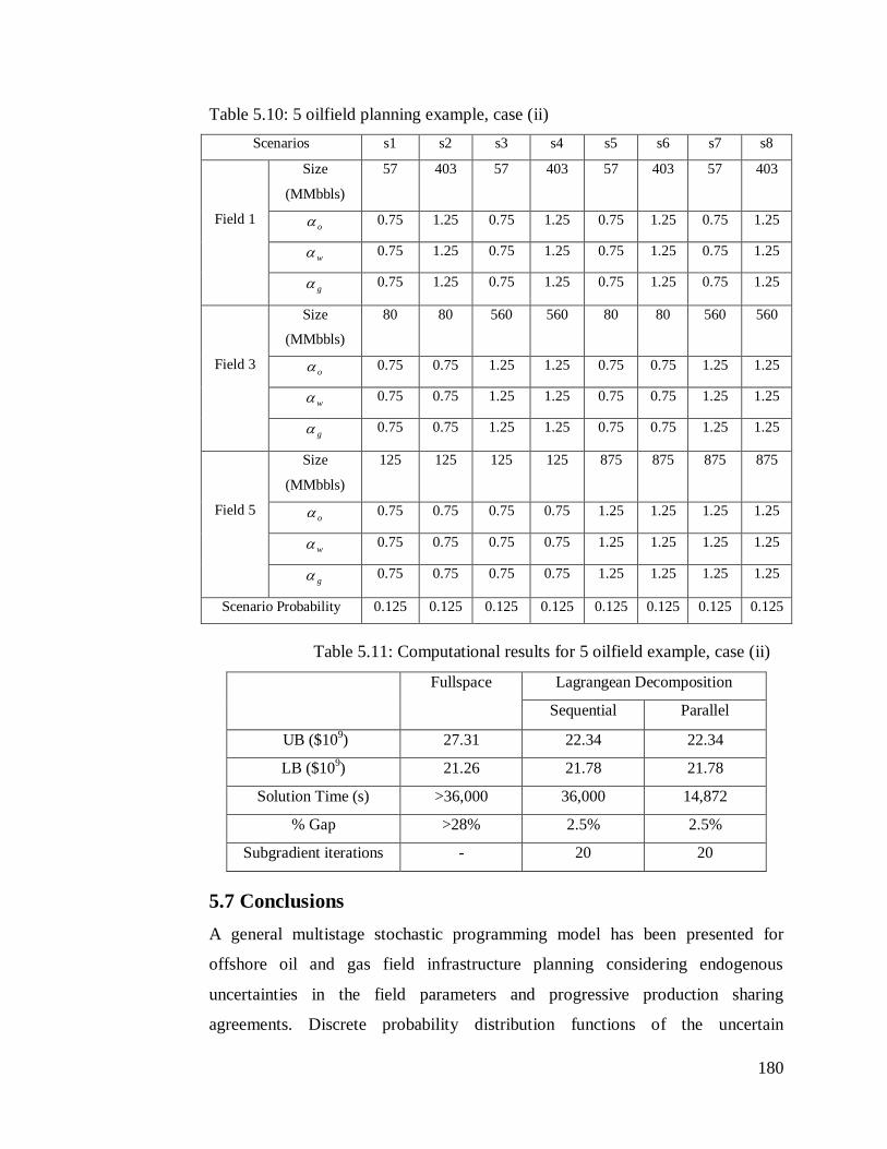
180

Table 5.10: 5 oilfield planning example, case (ii)

Scenarios s1 s2 s3 s4 s5 s6 s7 s8

Field 1

Size

(MMbbls)

57 403 57 403 57 403 57 403

o 0.75 1.25 0.75 1.25 0.75 1.25 0.75 1.25

w 0.75 1.25 0.75 1.25 0.75 1.25 0.75 1.25

g 0.75 1.25 0.75 1.25 0.75 1.25 0.75 1.25

Field 3

Size

(MMbbls)

80 80 560 560 80 80 560 560

o 0.75 0.75 1.25 1.25 0.75 0.75 1.25 1.25

w 0.75 0.75 1.25 1.25 0.75 0.75 1.25 1.25

g 0.75 0.75 1.25 1.25 0.75 0.75 1.25 1.25

Field 5

Size

(MMbbls)

125 125 125 125 875 875 875 875

o 0.75 0.75 0.75 0.75 1.25 1.25 1.25 1.25

w 0.75 0.75 0.75 0.75 1.25 1.25 1.25 1.25

g 0.75 0.75 0.75 0.75 1.25 1.25 1.25 1.25

Scenario Probability 0.125 0.125 0.125 0.125 0.125 0.125 0.125 0.125

Table 5.11: Computational results for 5 oilfield example, case (ii)


Sequential Parallel

UB ($109) 27.31 22.34 22.34

LB ($109) 21.26 21.78 21.78

Solution Time (s) >36,000 36,000 14,872

% Gap >28% 2.5% 2.5%


5.7 Conclusions

A general multistage stochastic programming model has been presented for

offshore oil and gas field infrastructure planning considering endogenous

uncertainties in the field parameters and progressive production sharing

agreements. Discrete probability distribution functions of the uncertain

181

parameters, i.e. field size, oil deliverability, water-oil-ratio and gas-oil ratio, are

considered to represent the scenarios where uncertainty in these parameters can

only be revealed once an investment is made in the field. The resulting decision-

dependent scenario tree is modeled using initial and conditional non-anticipativity

constraints considering the basic oilfield models developed in chapters 2 and 3.

The model yields optimum investment and operating decisions while maximizing

the expected NPV. Correlations among the endogenous uncertain parameters of a

field are considered, which reduce the dimensionality of the model for large

instances. The Lagrangean decomposition algorithm proposed in chapter 4 is

adapted to the corresponding multistage stochastic model for oilfield development

with parallel solution of the scenario subproblems. Numerical results on the two

oilfield development planning examples show that the proposed Lagrangean

decomposition algorithm, either sequential or parallel implementation, is efficient

as compared to the fullspace method, and allows the solution of intractable

instances of the problem. The model and solution approach can be further used as

a basis to incorporate additional complexities such as exogenous uncertainties in

oil/gas prices.

182

Chapter 6

A new decomposition algorithm for

multistage stochastic programs with

endogenous uncertainties

6.1 Introduction

In this chapter, we focus on type 2 of endogenous uncertainty for the multiperiod

planning problems where decisions are used to gain more information, and

resolve uncertainty either immediately or in a gradual manner. Therefore, the

resulting scenario tree is decision-dependent that requires modeling a

superstructure of all possible scenario trees that can occur based on the timing of

the decisions as observed in chapters 4 and 5. In this context, we focus here on a

general multistage stochastic programming framework to model the problems in

this class in which special disjunctive constraints with propositional logic are

considered to enforce the conditional non-anticipativity constraints that define the

decision-dependent scenario tree.

In general, these multistage stochastic programs (MSSP) become very

difficult to solve directly as deterministic equivalent since the problem size

(constraints and variables) increases with the number of scenarios, whereas the

solution time increases exponentially. Therefore, special solution techniques are

used to solve problems in this class. Several fullspace based approaches for the

medium-size problems exploiting the properties of the model and the optimal

solution have been proposed. In particular, Colvin and Maravelias (2010)

developed a branch-and-cut framework, while in chapter 4 we proposed a NAC

183

relaxation strategy to solve these MSSP problems under the assumption that only

few non-anticipativity constraints be active at the optimal solution.

Lagrangean decomposition is a widely used technique to solve large-scale

problems that have decomposable structure as in stochastic programs (Fisher,

1985; Ruszczynski, 1997; Carøe and Schultz, 1999; Guignard, 2003; Conejo et al.

2006). It addresses problems where a set of constraints links several smaller

subproblems. If these constraints are removed by dualizing them, the resulting

subproblems can be solved independently. In the case of multistage stochastic

programs with endogenous uncertainty initial and conditional non-anticipativity

constraints are the linking constraints, while each subproblem corresponds to the

problem for a given scenario. Therefore, the model has the decomposable

structure that is amenable to Lagrangean decomposition approaches. In this

context, a Lagrangean decomposition algorithm based on dualizing all the initial

NACs and relaxing all the conditional NACs that allow parallel solution of the

scenario subproblems has been proposed in chapter 4. An extended form of this

decomposition approach relying on the duality based branch and bound search is

also presented in Goel and Grossmann (2006), Tarhan et al. (2009), and Tarhan et

al. (2011) to close the gap between the upper and lower bounds. Solak (2007)

used a sample average approximation method for solving the problems in this

class, where the sample problems were solved through Lagrangean relaxation and

heuristics. However, there are several limitations with these methods including a

weak dual bound at the root node, a large number of iterations to converge at each

node, and many nodes that may be required during the branch and bound search

to close the gap depending on the branching rules and variables. Moreover, the

number of subproblems to be solved during each iteration at every node grows

linearly with the number of scenarios. In this chapter, we propose a new

decomposition scheme for solving these multistage stochastic programs that

overcomes some of the limitations of the standard approaches.

The outline of this chapter is as follows. First, in section 6.2 we introduce the

problem statement with particular focus on the problems where timing of

uncertainty realization depends on the optimization decisions. Then, a general

184

multistage stochastic mixed-integer linear disjunctive programming model for

endogenous uncertainty problems is presented in section 6.3. Several Lagrangean

decomposition approaches that have been used and their limitations are identified

next. To overcome these limitations, in section 6.5 we propose a new Lagrangean

decomposition scheme that relies on the concept of scenario group partitions. In

section 6.6, we present the computational results on process network and oilfield

planning problems adapted from chapters 4 and 5, respectively, to compare the

various decomposition approaches.


We consider multiperiod planning problems that have endogenous uncertainty in

some the parameters (type 2), i.e. where timing of uncertainty realization depends

on optimization decisions. In particular, the time horizon is represented by the

discrete set of time periods T = {1, 2, . . . . }. The set of endogenous uncertain

parameters ,....},{ 21 is considered where each parameter has a discrete set

of possible realizations. Therefore, a scenario s represents the possible

combination of the realizations of these uncertain parameters with a probability

sp . Note that when some of the parametersp are correlated as they may belong

to a particular uncertainty source, then the resulting scenario set will be smaller

(see chapter 5). The timing of uncertainty resolution in each uncertain parameter

depends on the decisions s

tx (both discrete and continuous) that have been

implemented so far. Furthermore, the uncertainty resolution rule can be

immediate (Goel and Grossmann, 2006) or gradual (Tarhan et al., 2009)

depending on the problem at hand. Therefore, the resulting scenario tree is

decision-dependent, and hence we need to use a superstructure of all possible

scenario-trees that can occur based on the decisions. In particular, we use logic

propositions and disjunctions as in chapter 4 (Goel and Grossmann, 2006; and

Gupta and Grossmann, 2011a) to represent the scenario-tree for the problems in

this class. The uncertainty realizations for each parameter p are assumed to be

time invariant. In the next section, we present a MSSP model corresponding to

this description.

185

6.3 Model

A multistage stochastic mixed-integer linear disjunctive program with

endogenous uncertainties can be represented in the following compact form:

(MD)

Ss Tt

s

tt

s xcpzmin (6.1)

staxAts s

t

t

ss ,..

(6.2)

SssTtxx I

s

t

s

t ',,' (6.3)

SssTtxxxFZ C

s

t

ssss

t ',,)....,( 121

', (6.4)

SssTtZ

xx

Z

C

ss

t

s

t

s

t

ss

t

',,',

'

',

(6.5)

',,}1,0{ Jjstxs

jt (6.6)

'\,, JJjstRxs

jt (6.7)

The objective function (6.1) in the above model (MD) minimizes the

expectation of an economic criterion over the set of scenarios Ss , and over a set

of time periods Tt . For a particular scenario s, inequality (6.2) represents

constraints that govern decisions s

tx in time period t and link decisions across

time periods. Non-anticipativity (NA) constraints for initial time periods TTI

are given by equations (6.3) for each scenario pair (s,s’) to ensure the same

decisions in all the scenarios. The conditional NA constraints are written for the

later time periods TTC in terms of logic propositions (6.4) and disjunctions

(6.5). Notice that the set of initial time periods IT may include the first few years

of the planning horizon until uncertainty cannot be revealed, while CT represents

the rest of the time periods in the planning horizon. The function )....,( 121

s

t

ss xxxF

in eq. (6.4) is an uncertainty resolution rule for a given pair of scenarios s and s’

that determines the value of the corresponding boolean variable ',ss

tZ based on the

186

decisions that have been implemented so far. The variable ',ss

tZ is further used in

disjunction (6.5) to ensure the same decisions in scenarios s and s’ if these are still

indistinguishable in time period t. Eqs. (6.6)-(6.7) define the domain of the

discrete and continuous variables in the model.

Notice that the model with reduced number of scenario pairs (s,s’) that are

sufficient to represent the non-anticipativity constraints can be obtained from

model (MD) after applying the three properties presented in the chapter 4. These

properties are defined on the basis of symmetry, adjacency and transitivity

relationship among the scenarios. The reduced model (MDR) can be formulated

as follows, where 3P is the set of minimum number of scenario pairs that are

required to represent non-anticipativity in each time period t,

(MDR)

Ss Tt

s

tt

s xcpzmin (6.1)

staxAts s

t

t

ss ,..

(6.2)

3

' )',(, PssTtxx I

s

t

s

t (6.3a)

3121

', )',(,)....,( PssTtxxxFZ C

s

t

ssss

t (6.4a)

3

',

'

',

)',(, PssTtZ

xx

Z

C

ss

t

s

t

s

t

ss

t

(6.5a)

',,}1,0{ Jjstxs

jt (6.6)

'\,, JJjstRxs

jt (6.7)

We then define the following sets,

p

k

kkk

p

ssssspssD

sssSssssssL

),...,,()',(}{)',(

,...,,...,,),...,,(

21

212121

(6.8)

'ˆˆ,)',( s

p

s

pppssD (6.9)

187

ppkkk LsssssssssP ),...,,(),(),....,,(),,( 21132213 (6.10)

Notice that the minimum scenario pair set 3)',( Pss can be obtained by first

defining a scenario group set pk Lsss ),....,,( 21 for each uncertain parameter p

with k realizations (eq. 6.8) such that the k scenarios in each of these

),....,,( 21 ksss set can only be realized at the same time irrespective of the other

realizations during the given time horizon. The basic idea to identify such

scenario sets ),....,,( 21 ksss is that all the scenarios in each of these sets only differ

in the realization of the uncertain parameter θp for which the corresponding set is

defined. Therefore, for any scenario pair ),....,,()',( 21 ksssss , the value of

pssD )',( where )',( ssD represents the index of the uncertain parameter

p in eq. (6.9) that distinguish the two scenarios s and s’ having values s

p

and 'ˆ s

p , respectively. The required minimum scenario pair set 3P (eq. 6.10) then

corresponds to the consecutive elements in the scenario group sets

pk Lsss ),....,,( 21 for each uncertain parameter p . The cardinality of the set 3P

is )(/1

SS as shown in chapter 4. For instance, if there are 2 uncertain

parameters, i.e. (θ1, θ2). Each of these uncertain parameters has three realizations

(L, M, H) which give rise to a total of 9 scenarios. The original model (MD)

requires a total of 72 scenario pairs to represent the non-anticipativity, while the

reduced model (MDR) only requires 12 scenario pairs, i.e. 123 P in each time

period t (see Gupta and Grossmann (2011a) for details).

The mixed-integer linear disjunctive model (MDR) can further be converted

to a mixed-integer linear programming model (MLR). First, the logic constraints

(6.4a) are re-written as the mixed-integer linear constraints eq. (6.4b) based on the

uncertainty resolution rule, where ',ss

tz is a binary variable that takes a value of 1

if scenario pair (s,s’) is indistinguishable in time period t, and zero otherwise. The

disjunction (6.5a) can then be converted to mixed-integer linear constraints (6.5b)

and (6.5c) using the big-M formulation. The resulting mixed-integer linear model

188

(MLR) includes constraints (6.1), (6.2), (6.3a), (6.4b), (6.5b), (6.5c), (6.6) and

(6.7).

3


s

t

ss

t

s

t

s

t

s

t (6.4b)

3


s

t

s

t

ss

t (6.5b)

3


s

t

s

t

ss

t (6.5c)

Figure 6.1: Structure of a typical Multistage Stochastic Program with Endogenous

uncertainties

Figure 6.1 represents the block angular structure of model (MLR), where we

can observe that the initial (eq. (6.3a)) and conditional (eqs. (6.4b), (6.5b) and

(6.5c)) non-anticipativity constraints link the scenario subproblems (eq. (6.2)), i.e.

these are the complicating constraints in the model. However, this structure

allows decomposing the fullspace problem into smaller subproblems by relaxing

the linking constraints. It should be noted that the NACs (especially conditional

NACs) represent a large fraction of the total constraints in the model.

6.4 Conventional Lagrangean Decomposition Algorithms

The reduced model (MLR) is composed of scenario subproblems connected

through initial (eq. (6.3a)) and conditional (eq. (6.4b), (6.5b) and (6.5c)) NA

constraints. If these NA constraints are either relaxed or dualized using

Scenario Constraints

Initial NACs

Conditional NACs

189

Lagrangean decomposition, then the problem decomposes into smaller

subproblems that can be solved independently for each scenario within an

iterative scheme for the multipliers as described in Carøe and Schultz (1999) and

in chapter 4. In this way, we can effectively decompose the large scale problems

in this class. However, there are several decomposition schemes that can be used

for this structure (Figure 6.1) as described below:

6.4.1 Lagrangean Decomposition based on relaxing conditional NACs

(Standard approach): In the decomposition algorithm of Figure 6.2 for MSSP

with endogenous uncertainties as proposed in chapter 4, the lower bound (LB) is

obtained by solving the Lagrangean problem with fixed multipliers',ss

t ,

(L1-MLR)

1 3)',(

'', )(minTt Pss

s

t

s

t

ss

t

Ss Tt

s

tt

s xxxcp (6.1a)

staxAts s

t

t

ss ,..

(6.2)

',,}1,0{ Jjstxs

jt (6.6)

'\,, JJjstRxs

jt (6.7)

which gives rise to the subproblems for each scenario Ss ,

(L1-MLRs)

1 3 3

')',(

'),'(

,'', )(minTt

ssPss

ssPss

ss

t

ss

t

s

t

Tt

s

tt

s xxcp (6.1b)

taxAts s

t

t

ss

.. (6.2a)

',}1,0{ Jjtxs

jt (6.6a)

'\, JJjtRxs

jt (6.7a)

In particular, the Lagrangean problem (L1-MLR) is formulated from the

mixed-integer linear reduced model (MLR) by relaxing all the conditional NA

constraints (6.4b), (6.5b) and (6.5c) and dualizing all the initial NA constraints

(6.3a) as penalty terms in the objective function. Figure 6.3 represents the

structure of the resulting model (L1-MLR). Notice that the each sub-problem

190

(L1-MLRs) in the Lagrangean problem (L1-MLR) corresponds to a scenario that

can be solved in parallel.

The upper bound (UB) is generated by using a heuristic based on the solution

of the Lagrangean problem (L1-MLR). In this heuristic, we fix the decisions

obtained from the above problem (L1-MLR) in the reduced problem (MLR) such

that there is no violation of NA constraints and solve it to obtain the upper bound.

The sub-gradient method by Fisher (1985) or an alternative update scheme (see

Mouret et al., 2011; Oliveira et al., 2013; and Tarhan et al. 2013) is used during

each iteration to update the Lagrangean multipliers. The algorithm stops when

either a maximum iteration/time limit is reached, or the difference between the

lower and upper bounds, LB and UB, is less than a pre-specified tolerance. Notice

that the extended form of this method relying on duality based branch and bound

search has also been proposed in Goel and Grossmann (2006); Tarhan et al.

(2009), and Tarhan et al. (2011) to close the gap between the upper and the lower

bounds.



LB = -∞

UB = ∞

Yes

Solve Lagrangean subproblem

with fixed multipliers to get LB

Gap < ε

or k > kmax

Stop

Find UB (Feasible Solution)


No




191

Figure 6.3: Lagrangean Decomposition based on relaxing conditional NACs

Limitations: We can observe from Figure 6.3 that the major limitation of this

Lagrangean Decomposition algorithm for endogenous uncertainty problems

(Gupta and Grossmann, 2011a; Goel and Grossmann, 2006; Tarhan et al., 2009;

and Tarhan et al., 2011) is that all the conditional non-anticipativity constraints

(6.4b), (6.5b) and (6.5c) are removed while formulating the scenario subproblems

at the root node. These constraints represent a large fraction of the total

constraints in the model and can have significant impact on the decisions. For

instance, in Figure 6.4, the scenario tree for the later time periods CT (conditional

NACs) can be constructed in several ways even though the initial NACs (for time

periods IT ) are satisfied.

Figure 6.4: Impact of conditional NACs on the scenario tree structure

Scenario

Subproblems

Dualize all

Initial NACs

Remove all

Conditional NACs

TI

TC

1 2 3,4 3,41,2 1,2 3 4 1 2 3 4

192

Therefore, there can be several undesired consequences that can occur with

this relaxation approach:

1. The dual bound at root node can be significantly weaker since a large amount

of information from the conditional NACs is ignored. In particular, only the

initial NAC are considered (dualized) while formulating the subproblems at

the root node, which represent only a first few time periods in the model. This

means that the dynamics of the problem corresponding to the later periods is

completely relaxed.

2. It is theoretically impossible to obtain a dual bound that is stronger than the

optimal solution of the model without all conditional NACs at the root node.

3. The total number of nodes in the branch and bound search tree and the number

of iterations required at each node can be very large.

4. Since many constraints are relaxed form the model, a good heuristic is needed

to generate a feasible solution based on the solution of the dual problem.

5. The number of subproblems grows with the number of uncertain parameters

and their realizations in an exponential manner.

6. It is problem specific and non-intuitive to define the branching rules/variables

in the tree search since there are several alternatives.

6.4.2 Lagrangean Decomposition based on dualizing all the NACs:

(i) In this decomposition approach, we dualize all the NACs (both initial

(6.3a) and conditional (6.5b) and (6.5c)) in the objective function directly while

formulating the lower bounding Lagrangean problem (L2-MLR), which is still

decomposable into individual scenarios. Notice that since (6.5b) and (6.5c) are

inequality constraints, the corresponding Lagrangean multipliers ',ss

tg and ',ss

tl

need to be non-negative.

(L2-MLR)

C

C

Tt Pss

ss

t

s

t

s

t

ss

tl

Tt Pss

ss

t

s

t

s

t

ss

tg

Tt Pss

s

t

s

t

ss

t

Ss Tt

s

tt

s

zMxx

zMxx

xxxcp

3

3

1 3

)',(

','',

)',(

','',

)',(

'',

))1((

))1((

)(min

(6.1c)

193

staxAts s

t

t

ss ,..

(6.2)

3


s

t

ss

t

s

t

s

t

s

t (6.4b)

',,}1,0{ Jjstxs

jt (6.6)

'\,, JJjstRxs

jt (6.7)

Figure 6.5 represents the structure of the model (L2-MLR) where L2-MLRs

correspond to the scenario sub-problems in this decomposed model.

(L2-MLRs)

C

C

Ttss

Pss

ss

tl

ss

tg

ss

t

ssPss

ss

tg

ss

tl

Ttss

Pss

ss

tg

ss

tl

s

t

Ttss

Pssss

Pss

ss

t

ss

t

s

t

Tt

s

tt

s

Mz

x

xxcp

')',(

',',',

'),'(

,','

')',(

',',

')',(

'),'(

,'',

3

33

1 3 3

)).).(1[(

])()([

)(min

(6.1d)

taxAts s

t

t

ss

.. (6.2a)

',)',(, 3

', ssPssTtdzCxB C

s

t

ss

t

s

t

s

t

s

t (6.4c)

',}1,0{ Jjtxs

jt (6.6a)

'\, JJjtRxs

jt (6.7a)

It is important to observe that we assign the shared binary variable ',ss

tz and

its corresponding constraints (6.4b) and objective function term to the scenario

problem s for all 3)',( Pss where (s < s’). This allows to decompose the problem

into independent scenarios. For instance in the case of 4 scenarios, the minimum

scenario pair set )}4,3(),4,2(),3,1(),2,1{(3 P and, therefore, the corresponding

shared variables 3,12,1 , tt zz are assigned to scenarios 1;

4,2

tz to scenario 2; and 4,3

tz

to scenario 3. As an alternative, one can also create a copy of the shared variable

',ss

tz as ss

tz ,' and its corresponding constraints (6.4b), (6.5b) and (6.5c) for all

194

3)',( Pss that will allow to keep these variables in both the sub-problems s and

s’. However, the performance of the two alternative decomposition approaches

should not be very different.

Figure 6.5: Lagrangean Decomposition based on dualizing all NACs directly

(ii) Another way to decompose the model (MLR) while considering all the

NACs, is based on first reformulating the constraints (6.3a), (6.5b) and (6.5c) as

(6.3b), (6.5d) and (6.5e) respectively, where ',~ ss

tx represents the value of the

variable 's

tx for 3)',(, PssTt .

3

', )',(,~ PssTtxx I

ss

t

s

t (6.3b)

3

',', )',(,~)1( PssTtxxzM C

ss

t

s

t

ss

t (6.5d)

3

',', )',(,~)1( PssTtxxzM C

ss

t

s

t

ss

t (6.5e)

',)',(,~3

',' ssPssTtxx ss

t

s

t (6.5f)

In addition, eq. (6.5f) is required to ensure that all the copy variables ',~ ss

tx for

's

tx have the same values in all the scenario pairs it occurs. Notice that the

reformulated model (MLRC) includes constraints (6.1), (6.2), (6.3b), (6.4b),

Scenario

Subproblems

Dualize all

Initial NACs

Dualize all

Conditional NACs

195

(6.5d), (6.5e), (6.5f), (6.6) and (6.7). Model (MLRC) can now be decomposed into

individual scenarios by dualizing only constraints (6.5f) as can be seen in Figure

6.6. L3-MLRC and L3-MLR

Cs represent the Lagrangean problem and scenario

sub-problems for this indirect decomposition approach, respectively.

Figure 6.6: Structure of the Reduced Model after reformulation (MLRC)

(L3-MLRC)

Tt

ssPss

ss

t

s

t

ss

t

Ss Tt

s

tt

s xxxcp

')',(

','',

3

)~(min (6.1e)

staxAts s

t

t

ss ,..

(6.2)

3

', )',(,~ PssTtxx I

ss

t

s

t (6.3b)

3

',', )',(,~)1( PssTtxxzM C

ss

t

s

t

ss

t (6.5d)

3

',', )',(,~)1( PssTtxxzM C

ss

t

s

t

ss

t (6.5e)

3


s

t

ss

t

s

t

s

t

s

t (6.4b)

',,}1,0{ Jjstxs

jt (6.6)

'\,, JJjstRxs

jt (6.7)

Scenario constraints

with corresponding NACs

((6.3b),(6.5d),(6.5e))

Equality

constraints (6.5f)

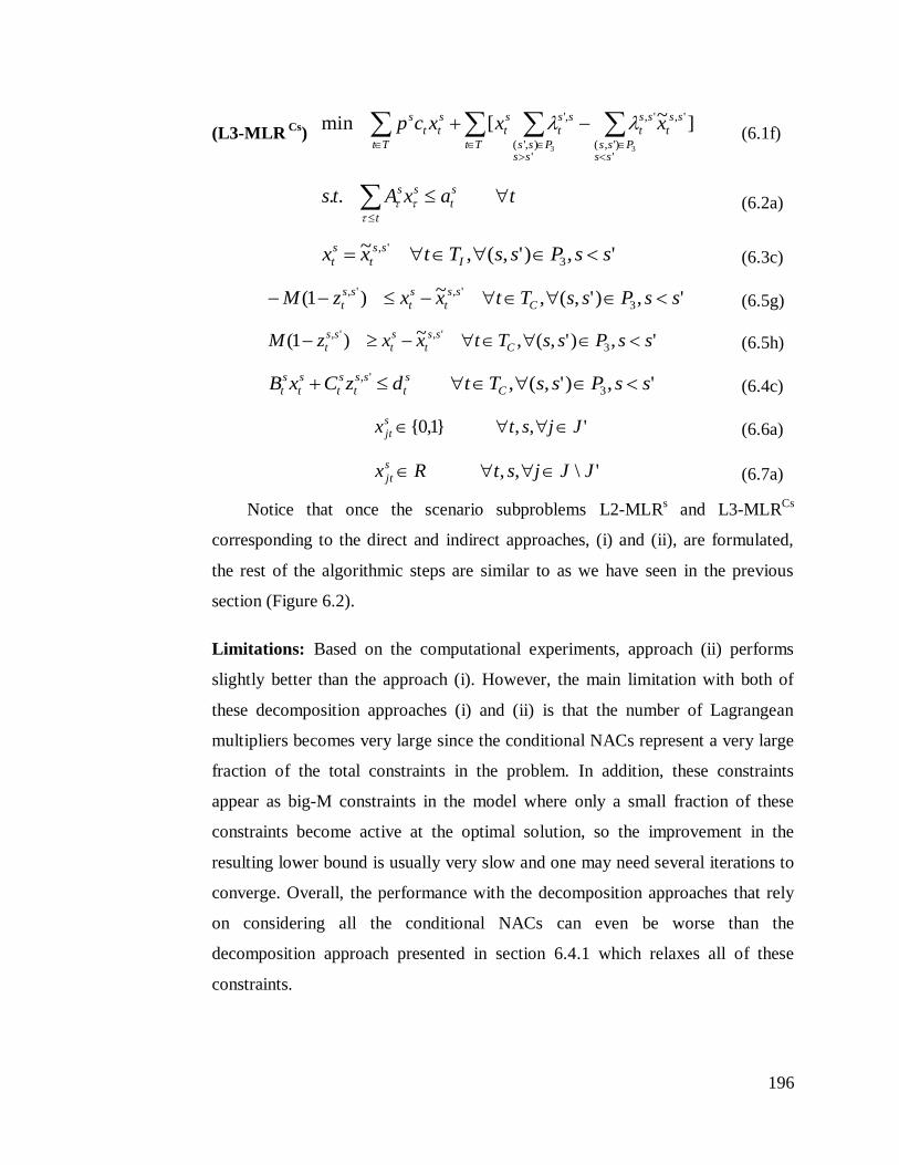
196

(L3-MLR Cs

) ]~[min

')',(

',',

'),'(

,'

33

ssPss

ss

t

ss

t

Ttss

Pss

ss

t

s

t

Tt

s

tt

s xxxcp (6.1f)

taxAts s

t

t

ss

.. (6.2a)

',)',(,~3

', ssPssTtxx I

ss

t

s

t (6.3c)

',)',(,~)1( 3

',', ssPssTtxxzM C

ss

t

s

t

ss

t (6.5g)

',)',(,~)1( 3

',', ssPssTtxxzM C

ss

t

s

t

ss

t (6.5h)

',)',(, 3

', ssPssTtdzCxB C

s

t

ss

t

s

t

s

t

s

t (6.4c)

',,}1,0{ Jjstxs

jt (6.6a)

'\,, JJjstRxs

jt (6.7a)

Notice that once the scenario subproblems L2-MLRs and L3-MLR

Cs

corresponding to the direct and indirect approaches, (i) and (ii), are formulated,

the rest of the algorithmic steps are similar to as we have seen in the previous

section (Figure 6.2).

Limitations: Based on the computational experiments, approach (ii) performs

slightly better than the approach (i). However, the main limitation with both of

these decomposition approaches (i) and (ii) is that the number of Lagrangean

multipliers becomes very large since the conditional NACs represent a very large

fraction of the total constraints in the problem. In addition, these constraints

appear as big-M constraints in the model where only a small fraction of these

constraints become active at the optimal solution, so the improvement in the

resulting lower bound is usually very slow and one may need several iterations to

converge. Overall, the performance with the decomposition approaches that rely

on considering all the conditional NACs can even be worse than the

decomposition approach presented in section 6.4.1 which relaxes all of these

constraints.

197

However, for the problems with exogenous uncertainties, there is no big-M

involved in the NACs. Therefore, on dualizing these NACs (all time periods) for

scenario decomposition, the quality of the lower bound is usually strengthened.

6.5 Proposed Lagrangean Decomposition Algorithm

The decomposition approaches presented in the previous section may perform

reasonably well for a certain class of problems with a given set of data. However,

as we mentioned these methods also have some limitations. To overcome them,

we propose a new decomposition scheme that neither relaxes nor dualizes all the

conditional NACs. The basic idea relies on decomposing the fullspace model into

scenario group subproblems instead of individual scenarios. This allows keeping a

subset of the NACs in the subproblems as constraints, while dualizing and

relaxing the rest of the NACs. Therefore, it can be considered as a partial

decomposition approach. Since, the formulation of the scenario groups is a key

element in the proposed decomposition algorithm, we first describe the

methodology to construct these scenario groups for the MSSP with endogenous

uncertainties.

6.5.1 Formulating the Scenario Groups: The proposed algorithm divides the

reduced model (MLR) into scenario group subproblems as explained in this

section. Let us consider that there are two endogenous uncertain parameters

},{ 21 where each one has 2 possible realizations (L, H). Therefore, there are 4

scenarios (1: LL, 2: HL, 3: LH, 4: HH). The scenario pairs (s,s’) required to

represent the NA constraints in each time period t based on the three properties

in chapter 4 are {(1,2),(1,3),(2,4),(3,4)} as can be seen in Figure 6.7(a). Notice

that the double line between scenario pairs is used to emphasize the fact that

there are initial as well as conditional NACs between each of these scenario

pairs, whereas each node represents the index of an individual scenario. The

dash lines correspond to the dualized NA constraints.

198

Figure 6.7: An illustration for the 4 Scenarios and its scenario group

decomposition (top view)

Figure 6.8: An illustration for the 4 Scenarios and its scenario group

decomposition (front view)

The Lagrangean decomposition scheme corresponding to the section 6.4.1 is

represented by Figure 6.7(b) where we remove all the conditional NACs and

dualize all the initial NACs. Figure 6.7(c) corresponds to the scenario

1

3

2

4

1

3

2

4

(a) (b) (c)

1

3

2

4

(e)

1

3

2

4

(d)

g1:(1,2)

g2:(3,4)

1

3

2

4

g2:(2,4)g1:(1,3)

TI

TC

s1 s2 s3 s4 s1 s2 s3 s4 s1 s2 s3 s4

s1 s2 s3 s4 s1 s2 s3 s4

TI

TC

(b)(a) (c)

(d) (e)

g1:(1,2) g2:(3,4) g1:(1,3) g2:(2,4)

199

decomposition scheme presented in section 6.4.2 that relies on dualizing all the

NACs (initial and conditional) either directly (i) or after reformulation (ii). In

contrast, the proposed algorithm decomposes the fullspace model into scenario

groups as shown in Figures 6.7(d) or 6.7(e). In particular, Figure 6.7(d)

corresponds to the two scenario group problems {g1: (1,2), g2: (3,4)} where

6.7(e) represents the scenario group problems { g1: (1,3), g2: (2,4)}. Notice that

Figures 6.7(a)-(e) correspond to the top view of the scenario-tree representation in

Figures 6.8(a)-(e), respectively. Each node in Figures 6.8(a-e) represents the state

of the system in a given time period t while the linking lines correspond to the NA

constraints.

The rules to formulate the scenario groups for the proposed algorithm are as

follows:

1. Each scenario s occurs in only one of the scenario group gS and every

scenario is included in at-least one of the groups G . All the scenario groups

GSg have equal number of scenarios. Therefore, the total number of

scenarios equal to the number of scenario groups times the number of

scenarios in each group i.e., gSGS . Notice that here we assume the

symmetry of the scenario groups to formulate the subproblems that have

almost similar complexity. However, we can always consider an asymmetric

approach as shown in Figure 6.9 for the 4 scenario instance described above.

Specifically, Figure 6.9(a) and 6.9(b) decompose the problem into two

scenario groups {g1: (1,2,3), g2: (4)} and {g1: (1,3,4), g2: (2)}, respectively,

where the subproblems with 3 scenarios should be more expensive to solve

than the one with a single scenario.

Figure 6.9: Asymmetric scenario group decomposition

(b)

1

3

2

4

(a)

g1:(1,2,3)

g2:(4)

1

3

2

4

g2:(2)

g1:(1,3,4)

200

2. Scenario groups gS are formulated by first selecting an endogenous uncertain

parameter and then taking those scenarios in a group which differ in the

realization of only that particular uncertain parameter. For instance, in Figure

6.7(a), we first select parameter }{ 1 and write only those scenario groups that

differ in the realization of this uncertain parameter, i.e. {(1,2),(3,4)} which

results in the scenario groups as in Figure 6.7(d). Similarly, the uncertain

parameter }{ 2 leads to the scenario groups {(1,3),(2,4)} in Figure 6.7(e).

Notice that these scenario groups are nothing but the scenario sets

pk Lsss ),....,,( 21 (eq. 6.8) that are required to formulate the reduced model

(MLR).

3. Since there can be many uncertain parameters }{ p each with its own

scenario set pk Lsss ),....,,( 21 , the selection of a particular set of scenario groups

is not unique.

(i) Ideally, one may consider selecting a scenario group set that provides

the tightest initial bound compared to the others. However, in general

unless all the combinations are tested, it is not obvious how to select

such a scenario group set.

(ii) A relatively simpler approach can be to first solve each scenario

independently, and selecting the scenario group set corresponding to

that uncertain parameter, which has the largest total difference in the

objective function values of the corresponding scenarios. This is due to

the fact that most likely the corresponding NACs for those scenarios

will be active at the optimal solution. Therefore, keeping these NACs

in the subproblem as constraints should yield a tighter bound. For

instance, select 7(e) if scenario group set corresponding to 2 exhibits

larger total variation in the objective function value than the scenario

group set for uncertain parameter 1 . In other words, this idea relies on

the sensitivity of the objective function value for an uncertain

parameter and its possible realizations.

201

Notice that for simplicity we only consider the cases with same

probabilities for all the scenarios during this work. If it would be possible, the

impact of different scenario probability values on scenario group partitions

will be addressed in our future paper.

4. Even after selecting a scenario group set that corresponds to an uncertain

parameter }{ p , it may still be difficult to solve the resulting scenario group

subproblems. For instance if a parameter has many realizations, then each

scenario group subproblem will have that many scenarios which may increase

the computational expense. Therefore, one may further divide the scenario

groups into subgroups and solve the resulting smaller problems.

Figure 6.10: 2 parameters, 16 scenarios and its scenario/scenario group

decomposition

As an example, say if we have 2 uncertain parameters and 4 realizations of

each parameter, there are a total of 16 scenarios. There are two possibilities of

the scenario groups {(1,2,3,4), (5,6,7,8), (9,10,11,12), (13,14,15,16)} (Figure

6.10(c)) and {(1,5,9,13), (2,6,10,14), (3,7,11,15), (4,8,12,16)} (Figure 6.10

(d)) according to the rules 1-3. Based on the problem characteristics, it may

be difficult to solve each scenario group subproblem with 4 scenarios.

Therefore, these groups can be further decomposed into a total of 8 scenario

(a) (b)

(c)

1

5

2

6

9 10

3

7

11

4

8

12

13 14 15 16

1

5

2

6

9 10

3

7

11

4

8

12

13 14 15 16

1

5

2

6

9 10

3

7

11

4

8

12

13 14 15 16

(d)

1

5

2

6

9 10

3

7

11

4

8

12

13 14 15 16

202

groups each with 2 scenarios, respectively (Figure 6.11(a) and 11(b)).

However, the quality of the bound may deteriorate since the corresponding

conditional NACs need to be relaxed. Therefore, there is a trade-off between

the quality of the bound and the complexity of solving a scenario group

problem.

Figure 6.11: Decomposition of the scenario groups into subgroups

5. In general, if the problem is expensive to solve for each scenario, it is better to use

scenario groups each with only few scenarios. On the other hand, if individual

scenarios are not expensive to solve, then one may consider more scenarios in

each group to improve the quality of the bound.

The above rules are general and can be applied to a problem with any

number of uncertain parameters and many realizations of each uncertain

parameter. For instance, Figure 6.12(a) represents the extension to three uncertain

parameter case where each parameter has 2 realizations (total 8 scenarios).

There are 6 possibilities to formulate the scenario groups in symmetric form:

(a) Taking 4 scenarios in each group:

{(1,2,3,4), (5,6,7,8)} i.e. Figure 6.12(c)

{(1,2,5,6), (3,4,7,8)} i.e. Figure 6.12(d)

{(1,3,5,7), (2,4,6,8)} i.e. Figure 6.12(e)

(b) Taking 2 scenarios in each group:

{(1,2),(3,4), (5,6),(7,8)} i.e. Figure 6.12(f)

{(1,5),(2,6), (3,7),(4,8)} i.e. Figure 6.12(g)

{(1,3),(2,4), (5,7),(6,8)} i.e. Figure 6.12(h)

1

5

2

6

9 10

3

7

11

4

8

12

13 14 15 16

1

5

2

6

9 10

3

7

11

4

8

12

13 14 15 16

(a) (b)

203

Figure 6.12: 3 parameters, 8 scenarios and its scenario/scenario group

decomposition

6.5.2 Decomposition Algorithm: Based on the scenario groups that are

constructed in the previous section, we now first present the corresponding

reformulated Reduced (MILP) model. Notice that these scenario group partitions

will be used to decompose the resulting reduced model into scenario group

subproblems during the proposed Lagrangean decomposition algorithm.

Let us consider that G is the set of scenario groups GS g that are selected

based on the rules presented in the previous section, where each of these scenario

groups gS may have 1 or more scenarios. The reduced model (MLR) can now be

represented as an equivalent model (MLRG) in terms of the scenario groups

GS g where we disaggregate the total NACs for the scenario pairs that

corresponds to the same scenario group gSss )',( (i.e. eqs. (6.3i),

(6.4i),(6.5i),(6.5j)) with those which belong to the different scenario groups

)'()( gg SsSs (i.e. eqs. (6.3j), (6.4j),(6.5k),(6.5l)).

(MLRG)

GS Ss Tt

s

tt

s

g g

xcpmin (6.1i)

2

1

4

3

5

6

7

8

2

1

4

3

5

6

7

8

2

1

4

3

5

6

7

8

2

1

4

3

5

6

7

8

2

1

4

3

5

6

7

8

2

1

4

3

5

6

7

8

2

1

4

3

5

6

7

8

(f)

(b) (c)(a) (d)

(g) (h)

2

1

4

3

5

6

7

8

(e)

204

GSstaxAts g

s

t

t

ss

,..

(6.2i)

GSssPssTtxx gI

s

t

s

t ',,)',(, 3

' (6.3i)

GSssPssTtdzCxB gC

s

t

ss

t

s

t

s

t

s

t ',,)',(, 3

', (6.4i)

GSssPssTtxxzM gC

s

t

s

t

ss

t ',,)',(,)1( 3

'', (6.5i)

GSssPssTtxxzM gC

s

t

s

t

ss

t ',,)',(,)1( 3

'', (6.5j)

GSSsSsPssTtxx gggI

s

t

s

t ),'()(,)',(, 3

' (6.3j)

GSSsSsPssTtdzCxB gggC

s

t

ss

t

s

t

s

t

s

t ),'()(,)',(, 3

', (6.4j)

GSSsSsPssTtxxzM gggC

s

t

s

t

ss

t ),'()(,)',(,)1( 3

'',

(6.5k)

GSSsSsPssTtxxzM gggC

s

t

s

t

ss

t ),'()(,)',(,)1( 3

'',

(6.5l)

',,}1,0{ JjGSstx g

s

jt (6.6i)

'\,, JJjGSstRx g

s

jt (6.7i)

The Lagrangean problem (L4-MLRG) corresponding to the model (MLR

G)

can be formulated by dualizing only those initial NAC constraints for the pairs of

scenarios (s,s’) that link the two scenario groups, i.e. eq. (6.3j), and removing the

corresponding conditional NACs (eqs. (6.4j),(6.5k) and (6.5l)). Therefore, the

initial and conditional NACs (eq. 6.3(i), 6.4(i), 6.5(i) and 6.5(j)) among the

scenario pairs (s,s’) that belong to the same scenario group remain in the

Lagrangean problem as explicit constraints.

(L4-MLRG)

GS Tt

SsSstsPss

s

t

s

t

ss

t

Ss Tt

s

tt

s

g

gg

g

xxxcp1 3

)'()(..)',(

'', )(min (6.1j)

205

GSstaxAts g

s

t

t

ss

,..

(6.2i)

GSssPssTtxx gI

s

t

s

t ',,)',(, 3

' (6.3i

GSssPssTtdzCxB gC

s

t

ss

t

s

t

s

t

s

t ',,)',(, 3

', (6.4i)

GSssPssTtxxzM gC

s

t

s

t

ss

t ',,)',(,)1( 3

'', (6.5i)

GSssPssTtxxzM gC

s

t

s

t

ss

t ',,)',(,)1( 3

'', (6.5j)

',,}1,0{ JjGSstx g

s

jt (6.6i)

'\,, JJjGSstRx g

s

jt (6.7i)

In contrast to the previous approaches, we can observe that the main idea in

the proposed decomposition approach is that instead of removing all the

conditional NACs from the model (as in section 6.4.1) or dualizing all the

conditional NACs either directly or in an indirect manner (as in section 6.4.2), we

only remove a subset of conditional NACs from the model and dualize a subset of

the initial NACs in the objective function instead of dualizing all the initial NACs

while formulating the Lagrangean problem (L4-MLRG). This results in the

decomposition of the reduced model (MLR) into scenario group subproblems

(L4-MLRGs

) rather than individual scenarios in the previous cases. Therefore, we

also refer it as a partial decomposition approach.

(L4-MLRGs

)

)(min

)'()(..',),'(

,'

)'()(..',)',(

',

31 3

gggg

g

SsSstsssPss

ss

t

TtSsSsts

ssPss

ss

t

s

t

Ss Tt

s

tt

s xxcp (6.1k)

g

s

t

t

ss SstaxAts

,..

(6.2k)

gI

s

t

s

t SssPssTtxx ',,)',(, 3

' (6.3k)

gC

s

t

ss

t

s

t

s

t

s

t SssPssTtdzCxB ',,)',(, 3

', (6.4k)

gC

s

t

s

t

ss

t SssPssTtxxzM ',,)',(,)1( 3

'', (6.5m)

gC

s

t

s

t

ss

t SssPssTtxxzM ',,)',(,)1( 3

'', (6.5n)

206

',,}1,0{ JjSstx g

s

jt (6.6k)

'\,, JJjSstRx g

s

jt (6.7k)

The structure of model (L4-MLRG) can be seen in Figure 6.13, where each

scenario group subproblem that contains its corresponding initial and conditional

NACs can be solved independently, and where only a small fraction of the total

initial and conditional NACs are dualized and removed, respectively. Since, the

resulting subproblems capture the more relevant information, i.e. the one

corresponding to the later time periods, the dual bound should be tighter.

Figure 6.13: Scenario decomposition approach in the proposed Lagrangean

Decomposition

We can then state the following proposition:

Proposition 6.1: The dual bound obtained from the proposed Lagrangean

problem (L4-MLRG) at root node is at-least as tight as the dual bound obtained

from the standard Lagrangean decomposition approach (L1-MLR) i.e. the

model (L1-MLR) is a relaxation of the model (L4-MLRG).

Proof: To prove this proposition it is sufficient to establish that,

(a) The feasible region of the proposed Lagrangean problem (L4-MLRG) is

contained within the feasible region of the model L1-MLR.

Scenario Group

Subproblems having

corresponding NACs

Dualize remaining

Initial NACs

Remove remaining

Conditional NACs

207

(b) The objective function value of the proposed Lagrangean problem (L4-

MLRG) over its feasible solutions

s

tx is at-least as large (assuming

minimization case) as the objective function value of the model L1-MLR.

For (a), since scenario constraints (6.2) in L1-MLR are equivalent to constraints

(6.2i) in L4-MLRG. Therefore, the only difference between both of these models

is that L4-MLRG has the additional constraints (6.3i), (6.4i), (6.5i) and (6.5j) in

the model. Hence, the feasible region of the model L4-MLRG

is contained within

the feasible region of the standard Lagrangean problem L1-MLR which has more

feasible solutions.

For (b), we first rewrite the model L1-MLR as L1-MLR’ where 0', ss

t

represent the Lagrangean multipliers corresponding to the dualized inequalities

)0( ' s

t

s

t xx and multipliers 0', ss

t correspond to the inequalities

)0( ' s

t

s

t xx . We use the inequality format of the initial NACs (eq. (6.3a)) to

dualize them in the objective function.

(L1-MLR’)

1 31 3 )',(

'',

)',(

'', )()(minTt Pss

s

t

s

t

ss

t

Tt Pss

s

t

s

t

ss

t

Ss Tt

s

tt

s xxxxxcp (6.1l)

s.t. (6.2), (6.6) and (6.7)

Similarly, model L4-MLRG can be rewritten as follows:

(L4-MLRG’

)

GS Tt

SsSstsPss

s

t

s

t

ss

t

TtSsSsts

Pss

s

t

s

t

ss

t

Ss Tt

s

tt

s

g

gggg

g

xxxxxcp1 31 3

)'()(..)',(

'',

)'()(..)',(

'', )()(min (6.1m)

s.t. (6.2i), (6.3i), (6.4i), (6.5i), (6.5j), (6.6i) and (6.7i)

On subtracting the objective functions (6.1l) and (6.1m), we have the following

summation,

GS Tt

SsSstsPss

s

t

s

t

ss

t

TtSsSsts

Pss

s

t

s

t

ss

t

g

gggg

xxxx1 31 3

)'()(..)',(

'',

)'()(..)',(

'', )()( (6.1n)

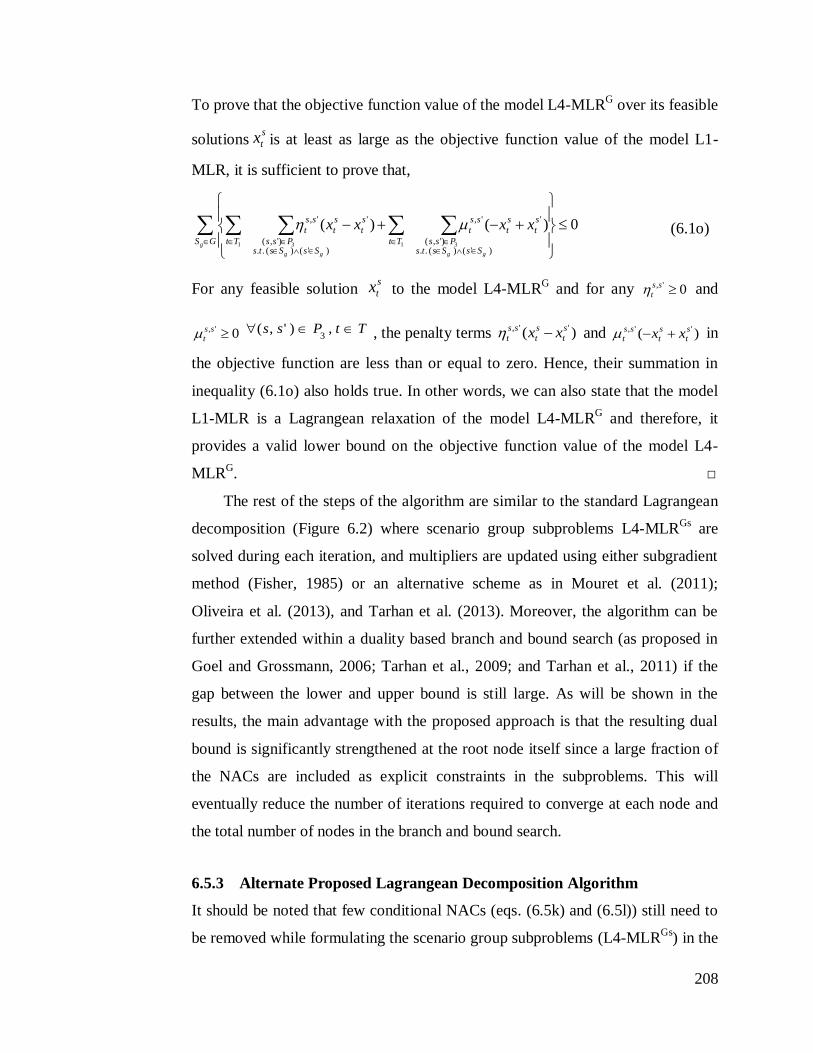
208

To prove that the objective function value of the model L4-MLRG over its feasible

solutionss

tx is at least as large as the objective function value of the model L1-

MLR, it is sufficient to prove that,

0)()(1 31 3

)'()(..)',(

'',

)'()(..)',(

'',

GS Tt

SsSstsPss

s

t

s

t

ss

t

TtSsSsts

Pss

s

t

s

t

ss

t

g

gggg

xxxx (6.1o)

For any feasible solution s

tx to the model L4-MLRG and for any 0', ss

t and

0', ss

tTtPss ,)',(

3 , the penalty terms )( '', s

t

s

t

ss

t xx and )( '', s

t

s

t

ss

t xx in

the objective function are less than or equal to zero. Hence, their summation in

inequality (6.1o) also holds true. In other words, we can also state that the model

L1-MLR is a Lagrangean relaxation of the model L4-MLRG and therefore, it

provides a valid lower bound on the objective function value of the model L4-

MLRG. □

The rest of the steps of the algorithm are similar to the standard Lagrangean

decomposition (Figure 6.2) where scenario group subproblems L4-MLRGs

are

solved during each iteration, and multipliers are updated using either subgradient

method (Fisher, 1985) or an alternative scheme as in Mouret et al. (2011);

Oliveira et al. (2013), and Tarhan et al. (2013). Moreover, the algorithm can be

further extended within a duality based branch and bound search (as proposed in

Goel and Grossmann, 2006; Tarhan et al., 2009; and Tarhan et al., 2011) if the

gap between the lower and upper bound is still large. As will be shown in the

results, the main advantage with the proposed approach is that the resulting dual

bound is significantly strengthened at the root node itself since a large fraction of

the NACs are included as explicit constraints in the subproblems. This will

eventually reduce the number of iterations required to converge at each node and

the total number of nodes in the branch and bound search.

6.5.3 Alternate Proposed Lagrangean Decomposition Algorithm

It should be noted that few conditional NACs (eqs. (6.5k) and (6.5l)) still need to

be removed while formulating the scenario group subproblems (L4-MLRGs

) in the

209

above method. Therefore, the best lower bound at the root node cannot be better

than the optimal solution of the model without these conditional NACs. To further

close the gap at the root node, we also propose an alternate Lagrangean

decomposition approach that may provide a stronger bound at the root node.

However, it involves solving more subproblems, and it may be computationally

more expensive than the proposed approach in the previous section. Therefore, it

is only useful for a certain class of problems.

The main idea is that we select all the scenario groups instead of a subset of

the scenario groups as we did in the previous section 6.5.1. However, since a

scenario can appear in more than one of these scenario groups, we need to equate

the decisions for this scenario in all of these scenario groups where it occurs. In

other words, we create a copy of each scenario for every scenario group problem

where it can appear and equating the decisions corresponding to all time periods

for that scenario for each of these scenario groups. The resulting model (Figure

6.14(b)) will be equivalent to the reduced model (MLR) (Figure 6.14(a)) where

{1’,2’,3’,4’} are the copy of the scenarios {1,2,3,4} and the connections between

them are the added equality constraints.

Therefore, to decompose the resulting problem (Figure 6.14(b)) into 4

scenario group subproblems {(1,2),(1’,3’),(2’,4’), (3,4)}, we dualize the equality

constraints correspond to each scenario and its copy variables, instead of

dualizing or removing the NAC constraints. This yields a set of 4 scenario group

subproblems (Figure 6.14(c)) i.e. {(1,2),(1’,3’),(2’,4’), (3,4)}. Since, none of the

conditional and initial NAC constraints are removed from the subproblems, the

bound is in general stronger. We can compare this decomposition with the

proposed one in Figure 6.7 where we obtain 2 scenario group problems.

Figure 6.14: Alternate proposed Lagrangean decomposition approach for 4

scenario problem

1

3

2

4

(a)

1

3

2

4

1’

3’ 4’

2’ 1

3

2

4

1’

3’ 4’

2’

(b) (c)

210

Qualitatively, this decomposition can be considered as the decomposition of

the reduced model (Figure 6.14(a)) at vertices as compared to the arcs in

standard/proposed decomposition described earlier. Notice that although this

alternate decomposition is computationally expensive since more subproblems are

involved than in the previous method, it can however be used in a hybrid scheme

with the proposed decomposition to improve the quality of lower bound. For

instance in Figure 6.10, we can first select the 4 scenario groups based on the

rules that are defined earlier, and then use this approach to further decompose

each group into subgroups by creating a copy of the scenarios in each of these

groups instead of the partitions used in Figure 6.11.


6.6.1 Process network planning under uncertain yield

Figure 6.15: 3 Process Network Example

Case (i): Planning of 3 process network over 10 years

To illustrate the application of the various decomposition approaches for

multistage stochastic programming with endogenous uncertainties, we consider

the following problem from Goel and Grossmann (2006). Given is a process

network (Figure 6.15) that is used to produce product A. Currently, the production

of A takes place only in Process III with installed capacity of 3 tons/hour and

yield of 0.70, that consumes an intermediate product B which is purchased. If

needed, the final product A can also be purchased so as to maintain its inventory.

The demand for the final product, which is known, must be satisfied for all time

periods over the given time horizon. Two new technologies (Process I and

Process II) are considered for producing the intermediate B from two different

ratey1

ratew1

ratey2

ratew2

ratew4

ratew5

ratey3

A B

B

B

B

C Process I

Process II

Process III

D

Purchases A

Sales A

Inventory A

211

raw materials C and D. These new technologies exhibit uncertainty in the yields.

The yield of Process I and Process II can take 2 discrete values each with equal

probability of 0.5. These two realizations of yield for each of Process I and

Process II give rise to a total of 4 scenarios (Table 6.1).

The problem consists of finding the expansion and operation decisions for

this process network for a 10 year planning horizon so as to minimize the total

expected cost of the project. The size of the resulting fullspace model (MLR) and

each individual scenario can be seen in Table 6.2 where the optimal expected cost

of the problem is $379,070. Notice that there is a significant increase in the total

number of constraints for the fullspace MSSP model due to the non-anticipativity

requirements.

Table 6.1: 3 Process Network Example (4 Scenarios)

Scenario s1 s2 s3 s4

Process I yield 0.69 0.81 0.69 0.81

Process II yield 0.65 0.65 0.85 0.85


Table 6.2: Model statistics for the 3 Process Network Example

After applying the various decomposition approaches, we obtain the results

shown in Figure 6.16 and Table 6.3, where an optimality tolerance of 1% and

maximum of 30 subgradient iterations (whichever comes first) are used as the

termination criteria. It can be observed that the proposed approach (section 6.5.2)

using SG2 scenario groups {(1,3),(2,4)} outperforms the other approaches since it

yields the tightest lower bound ($378,710) within 2 iterations (see Table 6.3). The

lower bound at the root node from the standard approach (section 6.4.1) after

many iterations is worse than the initial bound with the proposed approach

($375,880 vs. $377,290). In addition, the best upper bound from the proposed

Problem Type

Number of

Constraints

Continuous

Variables

Binary

Variables

Reduced Model (MLR) 1,869 845 120

Individual Scenario 192 202 30

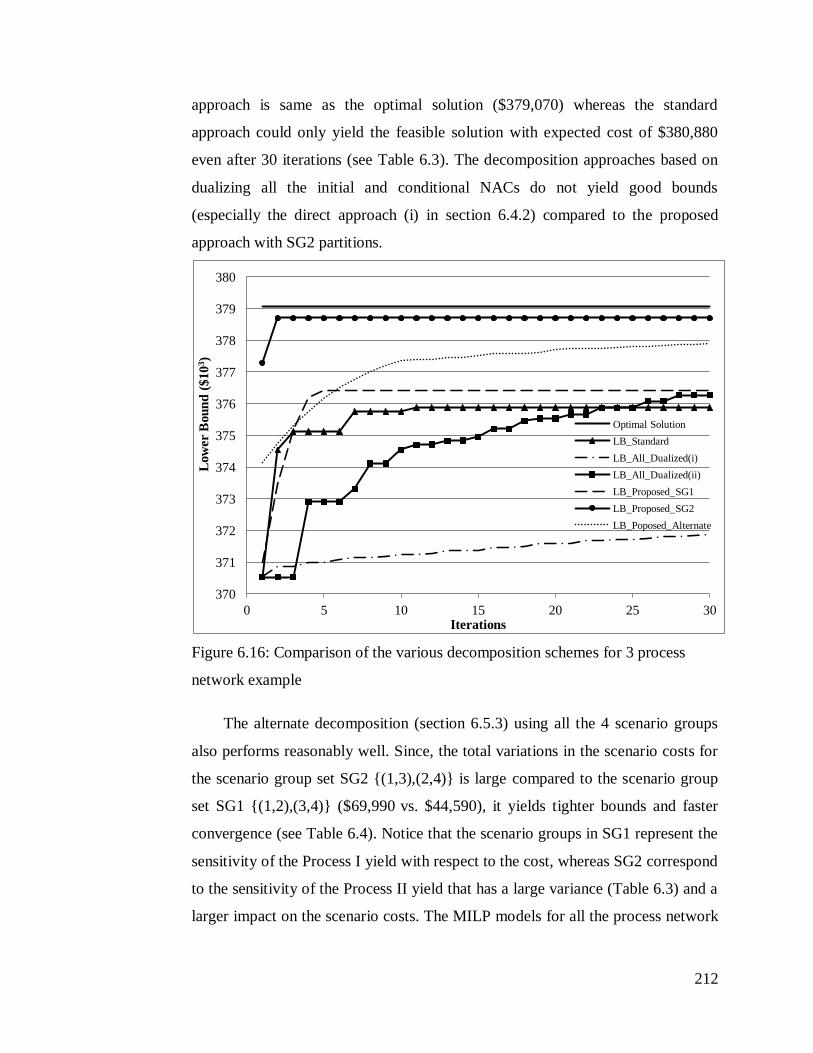
212

approach is same as the optimal solution ($379,070) whereas the standard

approach could only yield the feasible solution with expected cost of $380,880

even after 30 iterations (see Table 6.3). The decomposition approaches based on

dualizing all the initial and conditional NACs do not yield good bounds

(especially the direct approach (i) in section 6.4.2) compared to the proposed

approach with SG2 partitions.

Figure 6.16: Comparison of the various decomposition schemes for 3 process

network example

The alternate decomposition (section 6.5.3) using all the 4 scenario groups

also performs reasonably well. Since, the total variations in the scenario costs for

the scenario group set SG2 {(1,3),(2,4)} is large compared to the scenario group

set SG1 {(1,2),(3,4)} ($69,990 vs. $44,590), it yields tighter bounds and faster

convergence (see Table 6.4). Notice that the scenario groups in SG1 represent the

sensitivity of the Process I yield with respect to the cost, whereas SG2 correspond

to the sensitivity of the Process II yield that has a large variance (Table 6.3) and a

larger impact on the scenario costs. The MILP models for all the process network

370

371

372

373

374

375

376

377

378

379

380

0 5 10 15 20 25 30

Low

er B

ou

nd

($

10

3)

Iterations

Optimal Solution

LB_Standard

LB_All_Dualized(i)

LB_All_Dualized(ii)

LB_Proposed_SG1

LB_Proposed_SG2

LB_Poposed_Alternate

213

examples are implemented in GAMS 23.6.3 and run on Intel Core i7, 4GB RAM

machine using XPRESS 21.01 solver.

Table 6.3: Comparison of the various decomposition schemes for 3 Process

Network Example

Table 6.4: Variations in the objective function value with uncertain parameters(a)

Individual Scenario Costs (b) Scenario groups cost variations

Case (ii): Planning of 5 process network over 10 years

In this instance, we consider a 5 process network (Figure 6.17) having 3

uncertain parameters, i.e. yield of Process I, Process II, and Process V. Here we

consider 2 new additional processes compared to the previous example in which

Standard All Dualized

(i) direct

All Dualized

(ii) indirect

Proposed

SG1

Proposed

SG2

Proposed

Alternate

UB ($103) 380.88 380.88 380.88 380.88 379.07 379.07

LB ($103) 375.88 371.88 376.27 376.42 378.71 375.75

Solution Time (s) 8.89 5.24 9.51 5.86 0.94 2.12

% Gap 1.33% 2.42% 1.22% 1.19% <1% <1%

# iterations 30 30 30 30 2 4

Cost ($103)

s1 410.32

s2 365.73

s3 353.03

s4 353.03

SG1 SG2

s1-s2 44.59 -

s3-s4 0 -

s1-s3 - 57.29

s2-s4 - 12.70

Total cost

variations ($103) 44.59 69.99

B

B

B

C Process I

Process II D

Process IV E

A

B

B

Purchases A

Sales A

Inventory A

Process III

Process V

Figure 6.17: 5 Process Network Example

214

Process IV converts E into B with a yield of 0.75, and Process V that converts B

into final product A. Each of the uncertain yields has 2 realizations and gives rise

to a total of 8 scenarios with equal probabilities as shown in Table 6.5. The

problem consists of finding the expansion and operation decisions for this process

network over a 10 year planning horizon to minimize the total expected cost of

the project (see chapter 4 for details).

Table 6.5: 5 Process Network Example (4 Scenarios)

Scenario s1 s2 s3 s4 s5 s6 s7 s8

Process I yield 0.69 0.81 0.69 0.81 0.69 0.81 0.69 0.81

Process II yield 0.65 0.65 0.85 0.85 0.65 0.65 0.85 0.85

Process V yield 0.60 0.60 0.60 0.60 0.80 0.80 0.80 0.80

Scenario Probability 0.125 0.125 0.125 0.125 0.125 0.125 0.125 0.125

To use the proposed decomposition approach for this 8 scenario problem, we

partition the scenarios into scenario groups where each one has either 2 or 4

scenarios as in Figure 6.12. These scenario groups are denoted as follows:

(a) SG1: {(1,2),(3,4), (5,6),(7,8)}; SG2: {(1,5),(2,6), (3,7),(4,8)}; SG3:

{(1,3),(2,4), (5,7),(6,8)};

(b) SG4: {(1,2,3,4), (5,6,7,8)}; SG5: {(1,2,5,6), (3,4,7,8)}, and SG6: {(1,3,5,7),

(2,4,6,8)}

After applying the proposed decomposition approach (section 6.5.2) to these

6 scenario group sets, we can see from Figure 6.18 that the quality of the lower

bound improves from $357,920 (SG1) to $361,500 (SG6) as the total cost

variations for the corresponding scenario group set increases from $41,000 to

$224,810 as in the previous instance. Moreover, the bound obtained from the

larger subproblems having 4 scenarios (SG4, SG5, SG6) is tighter as compared to

the subproblems having 2 scenario each as in SG1, SG2 and SG3. This is due to

the fact that larger subproblems need only few conditional NACs to be relaxed

compared to the smaller subproblems. Table 6.6 and Figure 6.19 compare the

progress of the lower bounds, number of iterations and solution time required to

reach within 1% of optimality tolerance (or 30 iterations) for the standard and

proposed approaches with different scenario partitions. We can observe that

215

scenario group set SG6 outperforms other approaches since it provides the

strongest lower bound ($361,500) in just 2 iterations within 8.9s. Moreover, there

is a trade-off between the computational cost per iteration and the quality of the

bound obtained. It is interesting to note that in most of the cases, even the initial

bound using proposed scenario decompositions is much better than the final

bound from the standard approach ($355,180) and the rate of convergence to the

best possible dual bound is faster.

Table 6.6: Comparison of the standard vs. proposed approach for 5 process

network example

Figure 6.18: Variations in the scenario costs vs. bound obtained for different

scenario partitions

0

50

100

150

200

250

356

357

358

359

360

361

362

SG1 SG2 SG3 SG4 SG5 SG6

Tota

l C

ost

Varia

tion

s($

10

3)

Low

er B

ou

nd

($1

03)

Lower Bound

Total Cost

Variations

Standard Proposed

SG1

Proposed

SG2

Proposed

SG3

Proposed

SG4

Proposed

SG5

Proposed

SG6

UB ($103) 364.12 364.12 364.12 364.12 364.12 364.12 364.12

LB ($103) 355.18 357.92 358.08 358.62 360.82 361.35 361.50

Solution

Time (s)

16.32 24.59 15.38 20.40 7.63 12.44 8.9

% Gap 2.52% 1.73% 1.69% 1.53% <1% <1% <1%

# iterations 30 30 30 30 2 5 2

216

Figure 6.19: Comparison of the standard vs. proposed approach for 5 process

network example

6.6.2 Oilfield development planning under uncertain field parameters


346

348

350

352

354

356

358

360

362

364

366

0 5 10 15 20 25 30

Low

er B

ou

nd

($10

3)

Iterations

Optimal Solution

LB_Standard

LB_Proposed_SG1

LB_Proposed_SG2

LB_Proposed_SG3

LB_Proposed_SG4

LB_Proposed_SG5

LB_Proposed_SG6

FPSO 1 FPSO 3

Field 1

Field 3

Field 2

Total Oil/Gas Production

FPSO 2

217


In this instance, we consider 3 oilfields, 3 potential FPSO’s and 9 possible

connections among field-FPSO (Figure 6.20). A total of 30 wells can be drilled in

the fields and the planning horizon is 10 years. Field 3 has a recoverable oil

volume (field size) of 500 MMbbls. However, there is uncertainty in the size of

fields 1 and 2 where each one has two possible realizations (low, high) with equal

probability. Therefore, there are a total of 4 scenarios each with a probability of

0.25 (see Table 6.7). The problem is to determine the investment (FPSO


operating decisions (oil production rate) for this infrastructure with an objective to

maximize the total expected NPV (ENPV) over the planning horizon.

We consider the multistage stochastic MILP model presented in chapter 5 for

this oilfield development planning problem, which is an extension of the previous

deterministic model presented in chapter 2. The model for all the oilfield planning

instances are implemented in GAMS 23.6.3 and run on Intel Core i7, 4GB RAM

machine using CPLEX 12.2 solver. The optimal ENPV for this problem is $11.50

x109 when the reduced model (MLR) is solved in fullspace, and requires 1184s.

Table 6.8 represents the model statistics for this instance.

Table 6.7: 3 Oilfield Example (4 Scenarios), case (i)





Table 6.8: Model statistics for the 3 Oilfield Example, case (i)

Problem Type

Number of

Constraints

Continuous

Variables

Discrete

Variables

SOS1

Variables

Reduced Model (MLR) 16,473 9,717 876 240


218

Figure 6.21: Comparison of the various decomposition schemes for oilfield

example, case (i)

Figure 6.21 compares the performance of the upper bounds obtained at the

root node using standard Lagrangean decomposition based on dualizing the initial

NACs and removing the conditional NACs (section 6.4.1) with the decomposition

approaches proposed in section 6.5. A termination criterion of either 1% gap or 20

iterations is used. The proposed algorithm based on scenario groups SG1:

{(1,2),(3,4)} and SG2: {(1,3),(2,4)} yield stronger upper bounds, $11.59 x109 and

$11.56 x109 respectively, than the standard Lagrangean decomposition (section

6.4.1) ($11.62 x109). Additionally, the total computational effort is less with the

proposed approach since only 2 subproblems need to be solved at each iteration,

and only few iterations are needed to satisfy a 1% of optimality tolerance (Table

6.9). SG2 performs better than SG1 as can be observed from the total variations in

the scenario NPVs with respect to the change in the field sizes as calculated in

Table 6.10 ($6.63 x109 vs. $4.77 x10

9). This result is similar to the process

network example in the previous section. We can also observe that the alternate

proposed approach that considers 4 scenario groups (Figure 6.14(c)) performs

well but it is more expensive to solve (429s). It is important to see that the quality

11.45

11.50

11.55

11.60

11.65

11.70

11.75

11.80

11.85

0 5 10 15 20

Up

per B

ou

nd

($10

9)

Iterations

Optimal ENPV

UB_Standard

UB_Proposed_Alternate

UB_Proposed_SG1

UB_Proposed_SG2

219

of upper bound from SG2 is similar in the first iteration with the quality of UB

obtained from the scenario subproblems (section 6.4.1) after 20 iterations (see

Figure 6.21). Moreover, for clarity we only plotted the progress of the upper

bounds with iterations and the optimal NPV in Figure 6.21.

Table 6.9: Comparison of the various decomposition schemes for oilfield

example, case(i)

Standard Proposed SG1 Proposed SG2 Proposed Alternate

UB ($109) 11.62 11.59 11.56 11.58

LB ($109) 11.50 11.50 11.50 11.50

Solution Time

(s)

466 382 172 429

% Gap 1.02% <1% <1% <1%

# iterations 20 5 2 3

Table 6.10: Variations in the objective function value with uncertain parameters,

case (i)

(a) Individual Scenario NPV (b) Scenario groups NPV variations


scenarios)

In this case we consider uncertainty in the field size, oil deliverability, water-oil

ratio (WOR) and gas-oil-ratio (GOR) for oilfields 1 and 2. Notice that oil

deliverability, WOR and GOR are represented by the univariate polynomials in

terms of the fractional oil recovery as shown in equations (6.11)-(6.13)

respectively. The uncertainty in these parameters is characterized by the

corresponding parameters o , w and g . We assume that the uncertain

NPV ($109)

s1 8.95

s2 11.39

s3 12.32

s4 14.65

SG1 SG2

s1-s2 2.44 -

s3-s4 2.33 -

s1-s3 - 3.37

s2-s4 - 3.26

Total NPV

variations ($109) 4.77 6.63

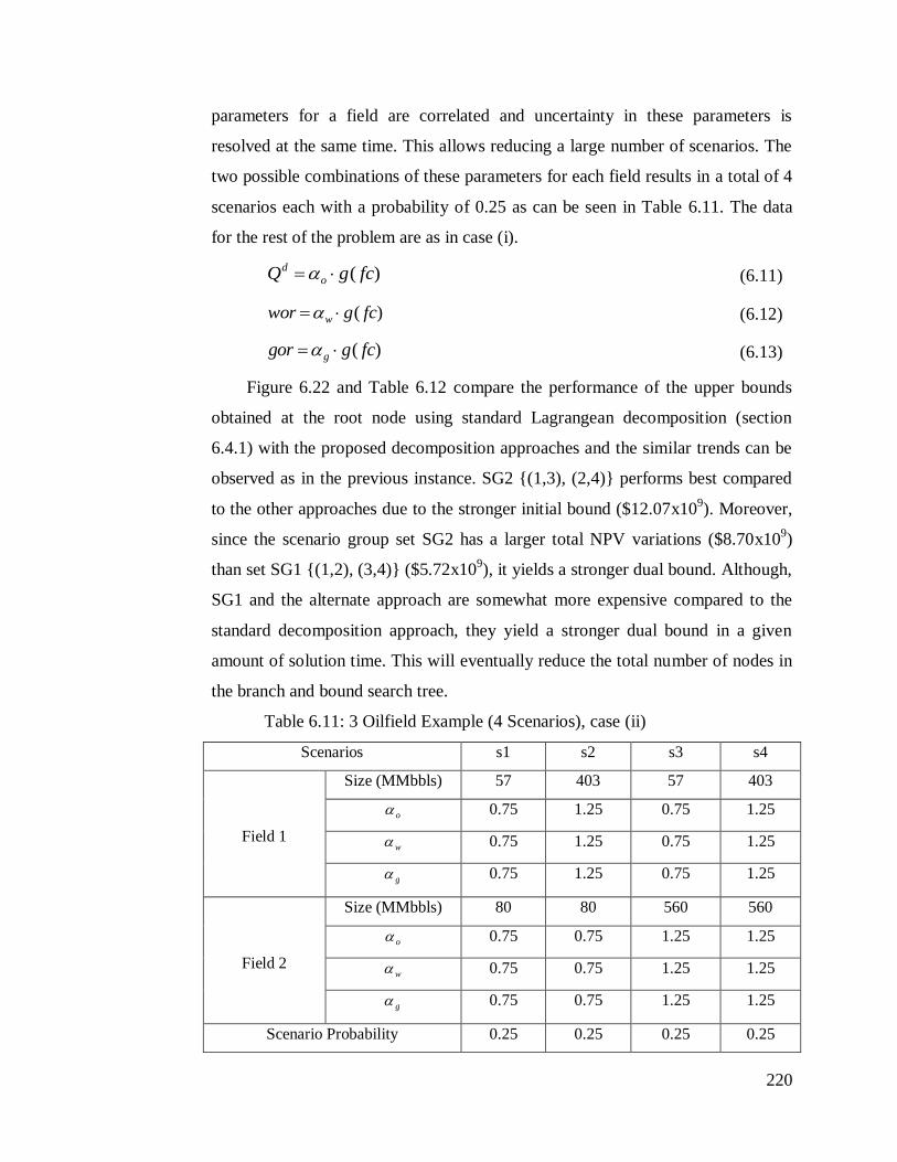
220

parameters for a field are correlated and uncertainty in these parameters is

resolved at the same time. This allows reducing a large number of scenarios. The

two possible combinations of these parameters for each field results in a total of 4

scenarios each with a probability of 0.25 as can be seen in Table 6.11. The data

for the rest of the problem are as in case (i).

)( fcgQ o

d (6.11)

)( fcgwor w (6.12)

)( fcggor g (6.13)

Figure 6.22 and Table 6.12 compare the performance of the upper bounds

obtained at the root node using standard Lagrangean decomposition (section

6.4.1) with the proposed decomposition approaches and the similar trends can be

observed as in the previous instance. SG2 {(1,3), (2,4)} performs best compared

to the other approaches due to the stronger initial bound ($12.07x109). Moreover,

since the scenario group set SG2 has a larger total NPV variations ($8.70x109)

than set SG1 {(1,2), (3,4)} ($5.72x109), it yields a stronger dual bound. Although,

SG1 and the alternate approach are somewhat more expensive compared to the

standard decomposition approach, they yield a stronger dual bound in a given

amount of solution time. This will eventually reduce the total number of nodes in

the branch and bound search tree.

Table 6.11: 3 Oilfield Example (4 Scenarios), case (ii)


Field 1

Size (MMbbls) 57 403 57 403

o 0.75 1.25 0.75 1.25

w 0.75 1.25 0.75 1.25

g 0.75 1.25 0.75 1.25

Field 2

Size (MMbbls) 80 80 560 560

o 0.75 0.75 1.25 1.25

w 0.75 0.75 1.25 1.25

g 0.75 0.75 1.25 1.25


221


example, case (ii)

Table 6.12: Comparison of the various decomposition schemes for oilfield

example, case(ii)

Case (iii) and (iv): Extension of the cases (i) and (ii), respectively, for 9

scenarios

In these instances we consider 3 realizations for each uncertain parameter (low,

medium, high) compared to two realizations (low, high) in the previous cases (i)

and (ii) of oilfield development problem. This results in the corresponding 9

scenario cases (iii) and (iv). Figures 6.23 and 6.24 compare the performance of

11.90

11.95

12.00

12.05

12.10

12.15

12.20

12.25

12.30

12.35

12.40

0 5 10 15 20

Up

per B

ou

nd

($

10

9)

Iterations

Optimal ENPV

UB_Standard

UB_Proposed_SG1

UB_Proposed_SG2

Standard Proposed SG1 Proposed SG2 Proposed Alternate

UB ($109) 12.14 12.10 12.07 12.06

LB ($109) 11.94 11.94 11.94 11.94

Solution Time (s) 438 1780 84 1045

% Gap 1.66% 1.28% <1% <1%

# iterations 20 20 1 5

222

the dual bounds at the root node from various decomposition schemes for these 3

oilfield and 9 scenario instances, whereas Table 6.13 summarizes the

computational results. Since the alternate decomposition (section 6.5.3) is very

expensive to solve for these cases, we only compare the proposed approach

relying on the scenario groups SG1 {(1,2,3),(4,5,6),(7,8,9)} and SG2

{(1,4,7),(2,5,8),(3,6,9)} with the standard approach (section 6.4.1). We can

observe that the initial bound with the proposed strategy ($11.93 x109) is much

better as compared to the final bound obtained from the standard Lagrangean

decomposition at the root node ($11.96 x109) for case (iii). It takes only 2 and 1

iterations in cases (iii) and (iv), respectively, for the proposed approach using set

SG2 to reach within 1% of optimality tolerance. On the other hand, the standard

and the proposed approach with set SG1 cannot reach within this gap even after

20 iterations or a given time limit of one hour.


example, case (iii)

11.60

11.70

11.80

11.90

12.00

12.10

12.20

12.30

12.40

0 5 10 15 20

Up

per B

ou

nd

($

10

9)

Iterations

Optimal ENPV

UB_Standard

UB_Proposed_SG1

UB_Proposed_SG2

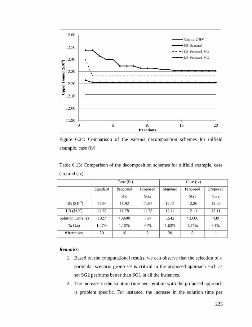
223


example, case (iv)

Table 6.13: Comparison of the decomposition schemes for oilfield example, case

(iii) and (iv)

Case (iii) Case (iv)

Standard Proposed

SG1

Proposed

SG2

Standard Proposed

SG1

Proposed

SG2

UB ($109) 11.96 11.92 11.88 12.31 12.26 12.23

LB ($109) 11.78 11.78 11.78 12.11 12.11 12.11

Solution Time (s) 1327 >3,600 764 1542 >3,600 439

% Gap 1.47% 1.15% <1% 1.62% 1.27% <1%

# iterations 20 10 2 20 8 1

Remarks:

1. Based on the computational results, we can observe that the selection of a

particular scenario group set is critical in the proposed approach such as

set SG2 performs better than SG1 in all the instances.

2. The increase in the solution time per iteration with the proposed approach

is problem specific. For instance, the increase in the solution time per

11.90

12.00

12.10

12.20

12.30

12.40

12.50

12.60

0 5 10 15 20

Up

per B

ou

nd

($10

9)

Iterations

Optimal ENPV

UB_Standard

UB_Proposed_SG1

UB_Proposed_SG2

224

iteration for the process networks examples is not that significant as in the

oilfield planning problem. Therefore, if the solution time per iteration for a

given problem increases drastically using the proposed decomposition,

then one may want to use the standard scenario based approach to explore

more nodes quickly in the branch and bound search tree or use

subproblems with smaller sizes in the proposed approach.

3. In general, for a given amount of the solution time the proposed approach

yields better dual bound and feasible solution as can be seen from the

numerical experiments. This is due to the fact that the increase in the

solution time per iteration is offset by the significant reduction in the total

number of iterations resulting in the lesser total solution time.

4. It should be noted that although the initial gap between lower and upper

bounds for the examples presented is not very large for the given data set.

However, based on Proposition 6.1 and computational experiments, we

can conclude that the performance of the proposed approach should be

similar for the large gap problems given that we select the scenario group

sets as described.

6.7 Conclusions

In this chapter, we have proposed a new approach for solving multistage

stochastic programs (MSSP) with endogenous uncertainties using Lagrangean

decomposition. The proposed approach relies on dividing the fullspace model into

scenario groups. Since the number of these scenario groups can be large, there are

several alternatives to select a particular set of scenario groups. Therefore, we also

presented few rules to identify and formulate a reasonable scenario group set that

can be used for the proposed partial decomposition approach within an iterative

scheme to update the multipliers. Specifically, the resulting subproblems involve

a subset of the NACs as explicit constraints while dualizing and relaxing the rest

of these constraints, which enhances the overall performance. An alternate

decomposition scheme that may even yield a tighter bound, but usually becomes

more expensive for the large cases, is also proposed.

225

The results on the process network and oilfield planning problems show that

the dual bound obtained at the root node from the proposed approaches are

stronger than the standard one used in chapters 4 and 5 since the impact of the

later time periods is also considered in the subproblems. Moreover, there is a

significant reduction in the number of iterations required to converge within a

specified tolerance. In most of the cases, even the initial bound with the proposed

approach is stronger than the corresponding final bound in the standard approach.

Given the tighter bound at the root node, the total number of potential nodes that

will be required in the branch and bound search should be smaller and branching

rules will be easier to identify. However, the solution time required per iteration

in the proposed approach is usually larger as compared to the standard approach,

but the difference is problem specific. Therefore, the comparison between the

qualities of the bounds obtained within a given amount of solution time should

also be considered while selecting a particular decomposition approach for the

problems in this class.

226

Chapter 7

Improving dual bound for

stochastic MILP models using

sensitivity analysis

7.1 Introduction

In this chapter, based on the previous work by Tarhan (2009), we introduce a

method to improve the dual bound during the solution of a general two-stage

stochastic mixed-integer linear programming model using dual decomposition

(Carøe and Schultz, 1999) and integer programming sensitivity analysis

(Dawande and Hooker, 2000). In particular, the method extracts the relevant

sensitivity information from the branch and bound tree of every scenario

subproblem, and uses that information to update the Lagrange multipliers and

improve the dual bound.

The outline of the chapter is as follows: In section 7.2, we introduce the two-

stage stochastic programming model under consideration and the standard

Lagrangean decomposition procedure to solve the model in the subsequent

section. To overcome the limitations of the standard approach, integer or mixed-

integer programming sensitivity analysis methods that will be used are introduced

in section 7.4. Sections 7.5 and 7.6 outline the procedure to combine the

sensitivity analysis with Lagrangean decomposition to improve the dual bounds of

stochastic integer or mixed-integer programming. Section 7.7 illustrates the

proposed method with numerical examples and compares it with the conventional

subgradient method.

227

7.2 Two-stage Stochastic programming

The main idea behind two-stage stochastic programming (see Figure 7.1) is that

we take some decisions (stage 1) here and now based on the possibility of future

outcomes of the uncertain parameters. While the rest of the decisions are stage -2

(recourse actions) decisions that are taken after uncertainty in those parameters is

revealed (e.g. low, medium or high scenarios). The objective is to minimize the

total cost of the first stage decisions and expected cost of the second stage

decisions.

Figure 7.1: Scenario tree for a two-stage stochastic programming

A typical two-stage stochastic mixed-integer linear (MILP) model (P-MILP)

involves discrete and continuous decisions in the first and/or second stages where

all the constraints and objective function are in linear or mixed-integer linear

form. Objective function (7.1) is the minimization of the expected cost over all

the scenarios s where sp is the probability of scenario s. First stage decisions sx

are taken here and now, while second stage decisions sy are taken after the

uncertainty is revealed. Constraints (7.2) and (7.3) correspond to each scenario

separately. To ensure that the first stage decisions are same for all the scenarios,

non-anticipativity (NA) constraints (7.4) are introduced in the model, which

makes the problem harder to solve since it couples all the scenarios. Constraints

(7.5)-(7.8) define the domain of the first and second stage variables. Reader

should refer to the nomenclature section at the end of this chapter.

Medium HighLow

Stage-1 decisions are

taken here and now

Scenario 1 Scenario 2 Scenario 3

Stage-2 decisions are

taken after uncertainty

gets revealed

228

(P-MILP) )(min ss

Ss

ss ydcxpz

(7.1)

SsaAxts s .. (7.2)

SsbTxyB ssss (7.3)

',',' ssSssxx ss (7.4)

', JjSsxs

j

(7.5)

'\, JJjSsRxs

j

(7.6)

', KkSsys

k

(7.7)

'\, KKkSsRys

k (7.8)

In general industrial planning, scheduling, supply-chain etc. problems under

uncertainty are formulated as a two-stage stochastic MILP shown above. These

problems become difficult to solve directly in practice since the problem size

increases (constraints and variables) with the number of scenarios, whereas the

solution time increasers exponentially. Therefore, special solution techniques are

used to solve the problems in this class.

Figure 7.2: Decomposable MILP model structure

Lagrangean decomposition is a widely used technique to solve the problems

that have similar decomposable structure as two-stage stochastic MILPs (see

Figure 7.2). It exploits the fact that there are certain set of constraints that make

subproblem 1

subproblem n

subproblem 2

Scenario

constraints are

in blocks

Non-anticipativity

constraints link the scenarios

(complicating constraints)

229

the problem harder to solve since it links the different small subproblems. If these

constraints are removed the resulting subproblems can be solved independently in

an efficient manner. In the case of two-stage stochastic MILPs, non-anticipativity

constraints (7.4) are the difficult constraint and each subproblem corresponds to

the scenario problem. Therefore, model (P-MILP) has the decomposable structure

that is required for the Lagrangean decomposition. In the next section we briefly

outline the conventional Lagrangean decomposition procedure.

7.3 Lagrangean Decomposition

Figure 7.3: Lagrangean Decomposition Algorithm (standard)

The standard Lagrangean decomposition approach involves three steps (see

Figure 7.3):

(a) Dualize complicating constraints in the objective function using

Lagrangean multipliers )( to decompose the problem into subproblems

(b) Solve each subproblem independently to obtain the lower bound (LB) on

the original problem and use a heuristic procedure to generate the feasible

solution i.e. an upper bound (UB)

Solve Lagrangean Problem

to obtain LB

Stop

UB

LB

Find UB by using a heuristic

Update Multipliers using

nonsmooth optimization

(e.g. subgradient method)

Initial Multipliers (0 )

k=0

No

Yes

Gap < ε or

k > kmax

230

(c) Based on the subproblem solutions and UB update the Lagrangean

multipliers )( using a non-smooth optimization (e.g. subgradient method)

for the next iteration

The procedure is repeated until the gap between upper and lower bound is

within a specified tolerance or a maximum iteration limit is reached. Due to the

presence of discrete variables, a duality gap may exist. Notice that if we dualize

the non-anticipativity constraints (7.4) in the objective function (7.1), problem (P-

MILP) decomposes into scenario subproblems (SP-MILP) and we can solve it

using Lagrangean decomposition.

(SP-MILP)

)])[(min'

,'

'

', sss

ss

sss

Ss ss

sss ydpxcpz

(7.9)

s.t. (7.2), (7.3), (7.5)-(7.8).

The main drawback of the above nonsmooth optimization approach used

within Lagrangean decomposition algorithm for MILPs (e.g. 2-stage stochastic) is

that only the optimal solution of each subproblem is considered while updating

the multipliers in each iteration. All the relevant information generated during

branch and bound algorithm while solving each subproblem is discarded. This

information could be useful to improve the lower bound efficiently. Therefore, the

total number of iterations required to reach convergence within the tolerance limit

is usually very large using the standard nonsmooth optimization approach such as

subgradient method (Fisher, 1985). In addition, it needs a heuristic procedure to

update the step size and an upper bound during each iteration. Overall, it may

result in slow convergence of the Lagrangean decomposition algorithm. There has

been some work done in this direction e.g. Bundle methods (Lemaréchal, 1974),

Volume algorithm (Barahona and Anbil, 2000), etc. However, the improvement in

the number of iterations is not very significant using these approaches. Our work

is motivated by using more information from each subproblem solution to

improve the performance of the Lagrangean decomposition algorithm. The main

goals of this work can be summarized as follow:

231

1. Extract the useful information from the branch and bound tree of each

subproblem during Lagrangean decomposition and use it to improve the

lower bound efficiently

2. Propose a new Lagrangean decomposition algorithm for MILP models

with decomposable structure (e.g. 2-stage stochastic) and benchmark the

results against the subgradient method

In the next section, we show that how the integer programming (IP)

sensitivity analysis can be used to extract useful information from the branch and

bound tree of each subproblem, and how it can further be used in the context of

Lagrangean decomposition algorithm to update the multipliers in each iteration.

Although we introduce the idea as a possible improvement over current stochastic

programming solution methods, the method is fairly general and can be applied to

a majority of the problems where Lagrangean decomposition is applicable.

7.4 Integer Programming (IP) Sensitivity Analysis

IP sensitivity Analysis (Primal Analysis and Dual Analysis) allow us to find valid

tight bounds for the objective function value when the objective function

coefficients are perturbed, using the information coming from the branch and

bound solution tree.

To understand this, let us consider that ( P ) is the original MILP model

whereas ( P ) is the perturbed problem after changing the objective function

coefficients from ( c ) to ( cc ). Given that ( P ) is an MILP, it is solved with a

branch and bound (or cut) method. The IP sensitivity analysis can be used to

calculate the range of the objective function value of the perturbed problem ( P )

without resolving this model. In particular, IP sensitivity analysis involves two

parts: Primal analysis and Dual analysis, which provide the upper and lower

bounds, respectively, on the perturbed problem ( P ).

Original Problem ( P ):

cxz min (7.10)

aAxts .. (7.11)

'Jjx j (7.12)

232

'\ JJjRx j

(7.13)

JjUxL jjj

(7.14)

Perturbed Problem ( P ):

xccz )(ˆmin (7.15)

s.t. (7.11) - (7.14)

Bounds on the perturbed problem using IP sensitivity analysis:

UBzLB ˆ

(7.16)

Dual Primal

Analysis Analysis

7.4.1 Primal Analysis

When the IP or MIP problem is solved using the branch and bound method, each

leaf node belongs to one of the following three sets of nodes (Figure 7.4):

N1: Set of nodes pruned by optimality (feasible integer solutions. e.g. node 3)

N2: Set of nodes pruned by bound (non-integer feasible solutions. e.g. node 1)

N3: Set of nodes pruned by infeasibility (leaf nodes pruned by infeasibility.

e.g. node 4)

Figure 7.4: A typical branch and bound solution tree for MILP

Primal Analysis says that the feasible solutions at any node in N1 stays

feasible (but not necessarily optimal) when the objective function coefficients

change to ( cc ). The best feasible solution is the minimum of the available

solutions. Therefore, the tightest upper bound on the objective function value of

+INF

+INF

-15

-15

+INF

-14.412

x3 = 1

+INF

-16.4

+INF

-17.364

x4 = 1x4 = 0

x3 = 0

0

1 2

3 4

233

the perturbed problem ( P ) can be obtained by solving the following optimization

problem (PA-LP) that uses the information from the feasible nodes (N1) of the

branch and bound solution tree of the original problem ( P ).

(PA-LP)

UBmax

(7.17)

Jj

j

n

jn NncvzUBts 1..

(7.18)

In particular, for the given optimal values of the variables jx at node n (i.e.

n

jv ) and perturbations jc the problem can be solved for the tightest upper bound

(UB ) on the perturbed problem. However, it should be noted that during the

proposed method jc will be treated as a variable instead of a parameter to obtain

the desired perturbations.

7.4.2 Dual Analysis

Dual analysis involves a set of linear constraints (DA-LP) that give the maximum

amount of decrease in the objective function value ( 0z ) when the objective

function coefficients are perturbed from c to cc , see Dawande and Hooker

(1998) for details. In particular, the analysis states that the lower bound on the

objective function value of the perturbed problem ( P ), i.e. LBzzz ˆ ,

remains valid if we can find free variables nr and n

js that satisfy the constraints

(7.19)-(7.24).

(DA-LP) 21)( NNnrvvsvc n

n

j

n

j

n

j

Jj

n

jj

(7.19)

1Nnzzavqr n

nn

j

Jj

n

jn

(7.20)

2Nnzzavqr n

nn

j

Jj

n

jn

(7.21)

21, NNnJjcs j

n

j

(7.22)

21, NNnJjqs n

j

n

j

(7.23)

234

where

cAq nn

j

(7.24)

Notice that the parameters n

jv (lower bound on variables), n

jv (upper bound

on variables) n (shadow price of the constraints), nz (objective value) and nz

(incumbent solution) at node n are obtained from the branch and bound solution

tree of the original problem ( P ). In addition to calculating the possible decrease

in the objective function value ( 0z ) for a given change in the objective

function coefficients ( c ), the analysis also allows us to find the possible

perturbations c that are allowed for a given value of z .

7.5 Application of IP Sensitivity Analysis for Multiplier Updating

in Two-stage Stochastic Programs

In this section, we explain how we combine the above integer programming

sensitivity analysis to extract the information from the branch and bound solution

tree of each scenario subproblem, and then update the multipliers during

Lagrangean decomposition for a two-stage stochastic MILP program. Notice that

here we consider two-stage stochastic MILPs having decomposable structure to

illustrate the proposed approach, but the method is general and can be applied to

any MILP model involving similar structure such as multistage stochastic, large

scale MILPs.

First, we can observe that in each iteration of the Lagrangean decomposition

algorithm (Figure 7.3) we update the multiplier values that only appear in the

objective function coefficients and resolve the resulting subproblems. Therefore,

eventually only the objective functions coefficients are perturbed during each

iteration (e.g. eq. (7.9)). This perturbation in the objective function coefficients

has direct correspondence to the perturbation that is explained in the IP sensitivity

analysis section above. For instance eq. (7.9) and (7.15) yield eq. (7.25).

ss

ss

ss

sssc'

,'

'

',

(7.25)

235

In addition, we also know that the integer programming sensitivity analysis

provides LB and UB on the perturbed problem objective value without resolving

it, by using the information from branch and bound tree of the original problem.

Based on these observations we extract the information required for

sensitivity analysis from the branch and bound tree of each subproblem during

Lagrangean decomposition. This additional information, rather than just the

optimal solution, can be used to construct a linear program that allow us to search

for those perturbations in the objective function coefficients (i.e. sc ) for the next

iteration that can potentially give us better directions and step size. The resulting

perturbations from such a linear program can therefore improve the lower bound

in an efficient manner than a simple nonsmooth optimization method.

(SA-LP) LBwUBw 21max

(7.26)

s

sUBUBts ..

(7.27)

Jj

kss

j

ksn

j

ks

ns kkNnSscvzUB }...3,2,1{,, ,

1

,,,

(7.28)

s

ss zzLB )(

(7.29)

sss

n

sn

j

sn

j

sn

j

Jj

sn

j

s

j NNnSsrvvsvc 21

,,,,,)(

(7.30)

sss

n

snsn

j

Jj

sn

j

s

n NnSszzavqr 1

,,, ,

(7.31)

sss

n

snsn

j

Jj

sn

j

s

n NnSszzavqr 2

,,, ,

(7.32)

sss

j

sn

j NNnJjSscs 21

, ,,

(7.33)

sssn

j

sn

j NNnJjSsqs 21

,, ,,

(7.34)

where cAq snsn

j ,,

(7.35)

SsJjcc s

jJj

s

j

,max

(7.36)

236

Therefore, the main idea now is to formulate such a multiplier updating

linear program (SA-LP) that maximizes a weighted sum of upper and lower

bounds generated by primal and dual analysis (7.26), while taking into account

the branch and bound tree information of the subproblem solutions from the

previous iteration. The reason for maximizing the sum of tightest possible upper

bound for each scenario is to move in the direction that overall improves the

lower bound on the original problem based on the feasible nodes that have been

explored so far. The idea to maximize the sum of lower bounds is to reduce the

possibility of decrease ( 0z ) in the current lower bound on the original

problem. This corresponds to minimizing the risk of finding a worse solution

when the model is re-optimized after the objective function coefficients are

changed to the values proposed by the method.

The proposed linear program (SA-LP) involves linear constraints (7.27)-

(7.28) and (7.29)-(7.35) that correspond to the primal and dual analysis,

respectively. The additional restriction (7.36) on the search space for the

perturbations is included to keep the LP solution bounded considering the fact that

all the feasible solutions for each subproblem are usually not explored in branch

and bound method and therefore the search space may be too relaxed. In

particular, we bound the s

jc value to be less than or equal to a fraction ( ) of

the maximum of the absolute value of objective function coefficients s

jc

corresponding to the duplicated variables to keep the search space neither very

restrictive nor relaxed.

Notice that the accumulation of the feasible nodes (N1) generated during the

previous iterations (k=1,2,….k-1) in the form of additional cuts (i.e. constraints

(7.28)) ensures that the search space for the new perturbations is restricted to only

to what has not been explored so far. It may potentially reduce the oscillations in

the lower bounds in successive iterations and reduce the number of iterations

required, while ensuring convergence. Notice that both sc and sz are variables

in the model that allow us to obtain the optimal multipliers values considering the

trade-offs associated with the potential improvement in the lower bound on the

237

original problem while minimizing the risk of deteriorations in the current lower

bound for these perturbations. The subjective parameters values ( ,, 21 ww ) are

explained in the results section.

7.6 Proposed Lagrangean Decomposition Algorithm

In comparison to the standard nonsmooth optimization method for multiplier

updating, the proposed Lagrangean decomposition algorithm for two-stage

stochastic programming involves solution of the linear program (SA-LP) during

each iteration as can be seen from Figure 7.5. Particularly, the proposed algorithm

allows us to extract the information from the branch and bound solution tree of

each subproblem using IP sensitivity analysis, and uses that information

constructively in the LP problem so that a better estimate of the Lagrangean

multipliers can be obtained as compared to a simple nonsmooth optimization

method.

Figure 7.5: Lagrangean Decomposition Algorithm (proposed)

Therefore, the algorithm has the potential to reduce the number of iterations

and the corresponding solution time, especially when each subproblem solution

(MILPs) is expensive. Moreover, it can also be applied to other decomposable

Solve Lagrangean Problem

to obtain LB

Stop

UB

LB

Find UB by using a heuristic

Update Multipliers using

proposed linear program

(SA-LP)

Initial Multipliers (0 )

k=0

No

Yes

Gap < ε or

k > kmax

238

MILPs. In the next section, we investigate the performance of the proposed

algorithm as compared to the subgradient method for two examples of two-stage

stochastic MILP models. Notice that we are not focusing on feasible solution

(UB) generation during this work since the idea is to improve the lower bound

efficiently. The upper bound can be calculated by using an efficient heuristic

procedure. In addition, comparison of the algorithm performance is in terms of

number of iterations since a basic branch and bound implementation is used for

subproblem solutions.


7.7.1 Example 1

We consider a two-stage stochastic integer program (7.37)-(7.42) from Carøe and

Schultz (1999) with uncertainty in the right-hand side of the constraints, i.e.

parameters ),( 21 . Two instances of the problem involving 3 and 50 scenarios

are generated based on the values of the uncertain parameters. The sizes of the

deterministic equivalent models are presented in Table 7.1. In the 3 scenario

instance, it is assumed that the uncertainty is represented by the three scenarios

)}12,15(),7,10(),8,5{(),( 21 with each one being equally likely. The optimal

solution of the problem with 3 scenarios is -64.33. For the larger instance having

50 scenarios, parameters have been sampled randomly and each scenario is

assumed to have equal probability.

),(45.1min 2121 xxQpxxSs

ss

(7.37)

]5,0[),(.. 21 xxts (7.38)

sssss yyyyxxQ 432121 28231916min),( (7.39)

114321 5432.. xyyyyts sssss (7.40)

224321 2316 xyyyy sssss (7.41)

}1,0{,,, 4321 ssss yyyy (7.42)

239

Table 7.1: Model statistics (deterministic equivalent) for Example 1 instances

Scenarios Discrete

Variables

Continuous

Variables

Constraints First Stage

Variables

Second Stage

Variables

3 18 0 12 6 12

50 300 0 2,550 100 200

In the proposed method, the sensitivity problem (SA-LP) is used to update

the multipliers during each iteration of the Lagrangean decomposition. In

particular, after solving each scenario independently all the necessary data (

snsnsn

j

sn

j

sn

nj

s

n

s

n

sss qvvvzzzNN ,,,,,

,,21 ,,,,,,,, ) for the sensitivity problem are extracted

and used in the model (SA-LP) to optimize. The result of the sensitivity problem

(SA-LP) proposes the multipliers (',ss ) and the resulting objective function

coefficients (s

jc ) that improve the dual bound. After some experience with the

method on a number of instances, we have set using the weights in the objective

function as 21 10ww and the value of parameter sp in eq. (7.36) throughout

all the examples.

On the other hand, during the subgradient iterations, a step length is

calculated using the solutions of scenario subproblems and prediction of the

optimal objective function value. Since we try to make the comparison between

methods as fair as possible, we have employed the optimal solution of the

example as predicted solution during the calculation of the stepsize in the

subgradient optimization. This gives subgradient method an advantage, but if the

proposed method performs better even under these conditions, then it will be a

clear evidence for potentially better performance in actual situations.

Both the methods are implemented in AIMMS 3.11 and problems are solved

using CPLEX 12.2 solver for all the instances. The initial multipliers are assumed

to be zero for both the approaches. The first subgradient iteration corresponds to

solving each scenario subproblem individually, which is also required for

generating the data for the model SA-LP. The methods have been compared over

iterations instead of solution time. The main reason is that during the time of

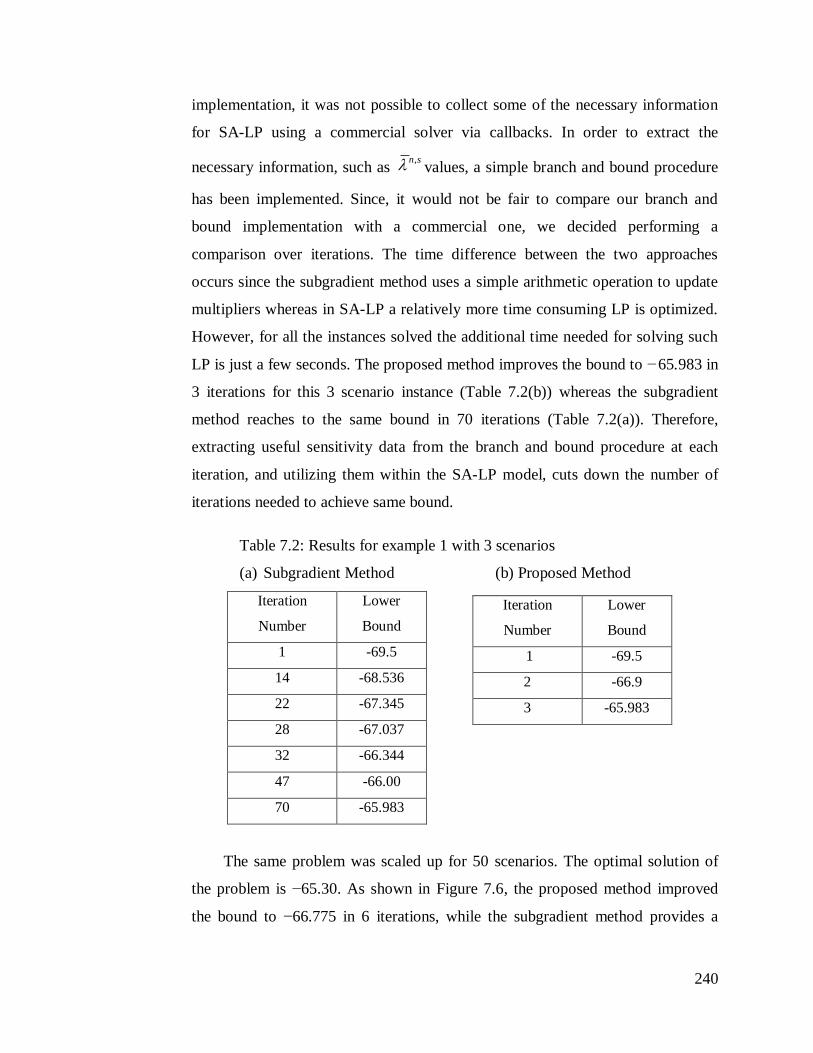
240

implementation, it was not possible to collect some of the necessary information

for SA-LP using a commercial solver via callbacks. In order to extract the

necessary information, such as sn, values, a simple branch and bound procedure

has been implemented. Since, it would not be fair to compare our branch and

bound implementation with a commercial one, we decided performing a

comparison over iterations. The time difference between the two approaches

occurs since the subgradient method uses a simple arithmetic operation to update

multipliers whereas in SA-LP a relatively more time consuming LP is optimized.

However, for all the instances solved the additional time needed for solving such

LP is just a few seconds. The proposed method improves the bound to −65.983 in

3 iterations for this 3 scenario instance (Table 7.2(b)) whereas the subgradient

method reaches to the same bound in 70 iterations (Table 7.2(a)). Therefore,

extracting useful sensitivity data from the branch and bound procedure at each

iteration, and utilizing them within the SA-LP model, cuts down the number of

iterations needed to achieve same bound.

Table 7.2: Results for example 1 with 3 scenarios

(a) Subgradient Method (b) Proposed Method

Iteration

Number

Lower

Bound

1 -69.5

14 -68.536

22 -67.345

28 -67.037

32 -66.344

47 -66.00

70 -65.983

The same problem was scaled up for 50 scenarios. The optimal solution of

the problem is −65.30. As shown in Figure 7.6, the proposed method improved

the bound to −66.775 in 6 iterations, while the subgradient method provides a

Iteration

Number

Lower

Bound

1 -69.5

2 -66.9

3 -65.983

241

dual bound of −66.761 in 75 iterations. Therefore, the method outperforms the

subgradient method in terms of the number of iterations.

Figure 7.6: Results for example 1 with 50 scenarios (Proposed vs. Subgradient

method)

7.7.2 Example 2 (Dynamic Capacity Allocation Problem (DCAP))

We investigate the performance of the proposed algorithm on Dynamic Capacity

Allocation Problem (DCAP) which is formulated as a two-stage stochastic MILP.

Data and problem details are adapted from Ahmed and Garcia (2003). This

problem has mixed-integer first-stage variables, pure binary second-stage

variables, and discrete distributions of the uncertain parameters. Uncertainty is in

the coefficient matrix of the constraints. Table 7.3 represents the sizes of the

deterministic equivalents for 2 problem instances (10 and 200 scenarios). Notice

that the fullspace problem is modeled in the extensive form considering NA

constraints (7.4).

Both instances (10 and 200 scenarios) are initially solved as fullspace

problems that yield the solutions 1571.682 and 1756.592, respectively. Given the

decomposable structure of this two-stage stochastic MILP problem, it is also

-230

-210

-190

-170

-150

-130

-110

-90

-70

-50

1 10 100

Dua

l Bou

nd

Iterations

Proposed Method (after Update 1 and 2)

Fullspace Solution

Subgradient Method

242

solved using the subgradient method as well as the proposed method. The results

in Figures 7.7 (a)-(b) show that the convergence of the subgradient method is

relatively slow and it takes more than 200 iterations to converge to the best

possible lower bound for both the instances.

Table 7.3: Model statistics (deterministic equivalent) for Example 2 (DCAP)

instances

Scenarios Discrete

Variables

Continuous

Variables

Constraints First Stage

Variables

Second Stage

Variables

10 330 60 840 120 270

200 6,600 1,200 2,44,800 2,400 5,400

In contrast, the proposed method converges in less than 10 iterations to yield

the solution of similar quality as the subgradient method for both the instances.

This more than an order of magnitude reduction in the number of iterations, is due

to the fact that during the subgradient method only the optimal solution of the

scenario subproblems is used to update the multipliers, whereas the proposed

method solves a linear program formulated using the information from the branch

and bound tree of each subproblem solution and search in the space of multipliers.

Notice that we use a higher weight on primal analysis as compared to the dual

analysis ( 101 w and 12 w ) and restrict the search space for perturbation based

on the probability of the scenario (i.e. sp ) during the proposed method as in

the previous example.

Remarks:

The solution time of the proposed linear program is negligible as compared

to the solution time of MILP subproblem. Therefore, the reduction in the number

of iterations using the proposed method dominates the additional cost of solving

the LP problem at each iteration. Moreover, for the models where each

subgradient iteration is expensive to perform due to many MILP subproblems to

be solved at each iteration, the proposed method can potentially decrease the total

solution time significantly since it reduces the number of iterations.

243

(a) 10 Scenario instance

(b) 200 Scenario instance

Figure 7.7: Results for example 2 (Proposed vs. Subgradient method)

1300

1350

1400

1450

1500

1550

1600

1 10 100

Dual

Boun

d

Iterations

10 Scenarios

Fullspace Solution

Subgradient Method

Proposed Method

(after Update 1 and 2)

1100

1200

1300

1400

1500

1600

1700

1800

1 10 100

Dual B

oun

d

Iterations

200 Scenarios

Fullspace Solution

Subgradient Method

Proposed Method

(after Update 1 and 2)

244

However, similar to other nonsmooth optimization methods, the proposed

method has some arbitrary components such as the weights assigned to primal (

1w ) and dual ( 2w ) bound in the objective function of SA-LP. The value of these

weights depends on the user’s experience with the proposed method. As explained

during the numerical examples, these weights were fixed as 21 10ww . Our

experience shows that the method performs well for various instances with

weights fixed at those values. We believe although such values are a good starting

point, more insight will be gained as the method is applied to other problems.

Moreover, there is a direct relation between the relative weight assigned to

the dual bound and the fraction of all feasible solutions explored in search tree. If

most of the feasible solutions are explored during the search process, then the

weight on dual bound can be much lower than weight on primal. In such a case,

for any value of ( s

jc ) the optimal solution is most likely be one of the feasible

solutions already explored in the search tree. Since in practice we do not

enumerate all possible solutions during the branch and bound search, we need a

nonnegative value for the dual weight and some bounds on ( s

jc ).

7.8 Conclusions

In this chapter, we have proposed a method for improving the dual bound of

decomposable MILP models using IP sensitivity analysis. In particular, a new

linear program is proposed based on the ideas of primal and dual analysis that

uses the information from branch and bound tree of each subproblem solution

during Lagrangean decomposition, and yields improved multipliers that results in

faster convergence of the algorithm. Based on the computational experiments on

two-stage stochastic MILPs, the method outperforms standard subgradient

method in terms of number of iterations (more than an order of magnitude

reduction). Given that a large number of subproblems (MILPs) are solved during

each iteration of the Lagrangean decomposition algorithm, the reduction in the

number of iterations can result in significant potential computational savings

where optimizing each of these subproblem takes a long time. Moreover, the

245

algorithm can be applied to more general classes of MILPs such as multistage

stochastic models, and MILPs with decomposable structure.

Nomenclature

A : matrix of constraint coefficients.

a : vector of right-hand-side coefficients.

c : vector of objective function coefficients.

jc : change in the objective function coefficient corresponding to variable jx

J : set of variables.

j : element of set J .

S : set of scenarios.

',ss : element of the set S .

LB : lower bound for the optimal solution of problem ( P ).

1N : set of leaf nodes pruned by optimality in branch and bound tree.

2N : set of leaf nodes pruned by bound in branch and bound tree.

3N : set of leaf nodes pruned by infeasibility in branch and bound tree.

n : element of sets 321 NNN .

nr : free variable.

n

js : free variable.

UB : upper bound for the optimal solution of problem ( P ).

n

jv : optimal value of variable jx at node n .

n

jv : upper bound for variable jx at node n .

n

jv : lower bound for variable jx at node n .

jx : continuous or discrete variable.

x : vector of variable jx .

nz : objective function value of node n in branch and bound tree.

nz : incumbent solution used for pruning node n .

246

z : optimal objective function value of the original model ( P ).

z : optimal objective function value of the perturbed model ( P ).

z : maximum allowable change in the objective function value. ( z ≥ 0)

n : vector of Lagrange multipliers found at node n during branch and bound

algorithm.

: parameter used for setting a bound on the change in the objective

function coefficients.

247

Chapter 8

Conclusions

In this thesis, we have developed new mixed-integer optimization models and

solution strategies for optimal development planning of offshore oil and gas field

infrastructure. Particularly, we considered a multi-field site with realistic

information in the planning such as fiscal rules of the agreements with the host

government and endogenous uncertainties in the field parameters. In chapters 2

and 3, we have proposed the deterministic models for the problem with/without

fiscal considerations. In chapter 4, we have presented a general multistage

stochastic programming framework and solution approaches for the endogenous

uncertainty problems, where timing of uncertainty realization is decision-

dependent. The deterministic oilfield planning models are then extended in

chapter 5 to include uncertainty in the field parameters relying on the ideas from

chapter 4. To improve the quality of the bounds during Lagrangean

decomposition in chapters 4 and 5, a new decomposition scheme is proposed in

chapter 6. Finally, in chapter 7 we introduced a new method for improving the

dual bound generated during the solution of a general two-stage stochastic mixed-

integer linear program.

8.1 An efficient multiperiod MINLP model for optimal planning

of offshore oil and gas field infrastructure

In chapter 2 we presented a novel deterministic mixed-integer nonlinear

programming (MINLP) model for offshore oil and gas infrastructure planning. As

compared to the previous work, the proposed realistic model considers multiple

fields, three components (oil, water and gas) explicitly in the formulation, facility

248

expansions decisions in the future, drilling rig limitations and nonlinear reservoir

profiles with an objective to maximize the net present value for the enterprise.

The decisions involve installation and expansion schedule of FPSO facilities and

respective oil, liquid and gas capacities, connection between the fields and

FPSO’s, well drilling schedule, and production rates of oil, water and gas in a

multiperiod setting to consider a long-term planning horizon incorporating several

economic trade-offs.

The major nonlinearities in the model are univariate polynomials and bilinear

terms (both involving continuous and discrete variables). In order to solve the

problem reliably, especially for the instances when more complex features are

incorporated into the model such as fiscal rules or uncertainties in the following

chapters, we first proposed to reformulate the MINLP formulation (Model 1)

using two new properties (see Appendix A). Using integration, the properties

allow representing the reservoir profiles in terms of the cumulative water and

cumulative gas produced as univariate polynomials rather than water-oil ratio and

gas-oil ratio and corresponding bilinear terms. Therefore, the new MINLP (Model

2) has nonlinearities only in term of the univariate polynomials and bilinear terms

involving discrete variables. The reformulation allows converting the MINLP

model to an MILP approximation (Model 3). In particular, the Model 2 has been

reformulated into an MILP using piecewise linearization and exact linearization

techniques with which the problem can now be solved to global optimality in a

more consistent manner. The proposed MINLP and MILP formulations are

further improved by using a binary reduction scheme based on the assumption

that the connection costs are relatively small compared to the other costs.

In terms of the numerical experiments on the proposed models, we

considered 3 realistic oilfield development instances involving up to 10 fields, 3

FPSO’s and 20 years planning horizon. The models were implemented in GAMS

23.6.3 and run on Intel Core i7 machine. In the first instance, we considered 3 oil

fields, 3 FPSOs, a total of 25 wells and the planning horizon of 10 years. Based

on the computational results, we observed that DICOPT performs best among

other MINLP solvers (e.g. SBB) in terms of computational time for Models 1 and

249

2. The number of OA iterations required was approximately 3-4 in both cases, and

solving Model 2 was slightly easier than solving Model 1 directly with this solver.

However, the solutions obtained were not guaranteed to be the global solution.

The global solver BARON 9.0.6 took more than 36,000s to be within ~10% of

optimality gap even for this small instance. The binary reduction scheme allowed

one third reduction in the number of binary variables for both models and a

significant decrease in the solution time. In contrast, the MILP Model 3 and its

binary reduction Model 3R that are formulated from Model 2 and Model 2R,

respectively, solved with CPLEX 12.2 and results showed the significant

reduction in the solution time after binary reduction (6.55s vs. 37.03s), while both

the models gave the same optimal NPV i.e. $7030.90M. Notice that the

approximate MILP models are solved to global optimality in few seconds, while

global solution of the original MINLP formulations is much more expensive to

obtain. The MILP solution was further used to improve the quality of local

solutions obtained from the MINLP formulations. Similar trends were observed

for the other two larger instances.

Therefore, it can be concluded that while the proposed MINLP models may

sometimes lead to near optimal solutions, the MILP approximation is an effective

way to consistently obtain these solutions. These MILP solutions also provide a

way to assess the quality of suboptimal solutions from the MINLPs, or finding

optimal or near optimal solutions by using the discrete decisions from this model.

None of the MINLP solvers could find better solutions than the ones obtained

using the MILP solution within a certain amount of time. Moreover, the solutions

from the convex MINLP solvers can be sub-optimal when we extend it to more

complex cases (chapter 3), and they cannot provide any guarantees of the valid

upper bound in the Lagrangean decomposition unless each subproblem is solved

to global optimality (chapter 5). Therefore, we used the MILP model for including

complex fiscal rules and/or uncertainties in the subsequent chapters.

The results of the chapter led to many challenges that need to be addressed.

The global solution of the proposed MINLP models is expensive using a state-of-

the-art solver directly. Therefore, the models can be used as a basis to develop

250

global optimization based approaches even though the MINLP solvers that rely on

convexity assumption can yield good solutions in an ad-hoc manner. The MILP

approximate model can be solved to global optimality using more reliable

commercial MILP solvers. However, the solution time for the realistic instances is

still large, especially if we consider many point estimates for the polynomials.

Therefore, a more reliable approximation scheme or a decomposition approach

such as a bi-level decomposition algorithm can be investigated to reduce the total

computational effort while maintaining the solution quality.

8.2 Modeling and computational strategies for optimal

development planning of offshore oilfields under complex

fiscal rules

In chapter 3, we extended the deterministic models presented in chapter 2 for

offshore oil and gas field infrastructure planning to incorporate complex fiscal

rules of the agreements with the host government. In particular, we considered

progressive production sharing agreements with ringfencing provisions in the

proposed general model so that it can be used as a basis to represent a variety of

contracts used in the industry. The fiscal model considers the trade-offs between

optimal investment and operating decisions and resulting NPV for the oil

company after paying government share, and yields improved decisions compared

to a simple NPV based optimization used in chapter 2. However, the major

challenge with this extension is that the computational expense increases

significantly mainly due to the progressive nature of the profit share, and the

ringfencing provisions. In particular, additional binary variables need to be

introduced to represent the tiers that define the progressive terms, and the

relaxation of the model is generally weak due to the absence of the good bounds

on the variables. Therefore, we have also proposed a tighter formulation (Model

3RF-L) by introducing additional logic constraints and valid inequalities in the

model that improve the relaxation and reduce the branch and bound search tree.

Heuristic approaches that relax and approximate the sliding scale terms, Model

251

3RI and Model 3RI-A, respectively, in the form of simple linear inequalities are

also proposed to obtain the reasonable solutions for the large instances.

To illustrate the impact of the fiscal terms and the proposed approaches, we

considered three instances of the realistic oilfield planning problem involving

progressive production sharing agreements. The models were implemented in

GAMS 23.6.3 and run on Intel Core i7, 4GB RAM machine using CPLEX 12.2.

Instance 1 did not involve ringfencing provisions, while instances 2 and 3 were

solved with and without ringfencing provisions to illustrate the additional

computational cost associated to these provisions. The first instance considered 3

fields, 3 FPSOs, a total of 25 wells that can be drilled, and 15 years planning

horizon. The sequential approach that first maximizes NPV, i.e. Model 3, and

then calculates the contractor share based on these decisions and fiscal rules

yields a total NPV of $1362.67M, which is significantly lower than the optimal

solution ($1497.69M) of the model with fiscal considerations (Model 3F). In

addition, investment and operating decisions were also very different, i.e. mostly

front ended in the case of sequential approach. This is due to the optimistic nature

of the sequential approach that tries to generate as much revenue as possible at the

beginning of the planning horizon, neglecting the trade-offs that are associated to

the fiscal part. Therefore, it may lead to the decisions that can incur large losses in

the long term after considering the impact of the fiscal calculations since higher

tiers (higher tax rates) become active in the earlier years during the planning

horizon. Model 3RF which is obtained after binary reduction from Model 3F

yields the same solution in an order of magnitude less time (337s vs. 3,359s). In

contrast, solving the corresponding MINLP formulation Model 2F with BARON

9.0.6 could only provide a solution having NPV of $1198.44M with a 60% gap in

more than 10 hours. Moreover, we observed that solving Model 2F directly with

DICOPT requires a good initialization due to the additional binary variables and

constraints that are added in this fiscal model compared to Model 2. Therefore,

the optimal solution from the corresponding MILP formulations (Model 3F and

Model 3RF) provides optimal or near optimal solutions of the original Model 2F.

We fixed the design decisions in Model 2F from the optimal solution of Model

252

3RF, and solved the resulting NLP problem that yields an NPV of $1496.26 M,

which shows that the accuracy of the MILP solution is within 0.1% of the MINLP

formulation. Therefore, the proposed MILP formulations performed very

efficiently and provided near optimal solutions.

Similarly, significant savings and different decisions were obtained with

fiscal considerations during planning for instance 2 having 5 fields and 20 years

of time horizon. The tighter formulation Model 3RF-L is solved in one fourth of

the time than Model 3RF. The relaxed Model 3RI was solved more than 20 times

faster than the original Model 3RF, while the approximate Model 3RI-A took

only 82s as compared to Model 3RF (1164s), and yielded the optimal solution

after we fixed the decisions from this model in the original one. Both the relaxed

and approximate models were even ~3 times faster than the model without any

fiscal terms (Model 3R) that took 190s. We also considered two ringfences for

instance 2 where progressive PSA terms were defined for each of these ringfences

separately. We observed that including ringfencing provisions made Model 3RF

expensive to solve (>10 hrs) compared to the one without any ringfences that

required only 1,164s. This is due to the additional binary variables that were

required in the model for each of the two ringfences, their trade-offs and FPSO

cost disaggregations. In contrast, since Models 3RI and 3RI-A did not require

binary variables for the sliding scale in disjunction (3.30), they solved much faster

than Model 3RF (>300 times faster) and Model 3RF-L (~30 times faster).

Preliminary results on a bi-level decomposition approach were also presented for

this instance that provided the rigorous bounds on the objective function value for

the fiscal model involving ringfencing provisions. The largest instance we solved

involves 10 oil fields, 3 FPSOs, a total of 84 wells, 20 years planning horizon, and

3 ringfences.

The main conclusion that can be drawn from this chapter is that the explicit

consideration of the fiscal rules is important for the oilfield infrastructure

planning instead trying to solve a simple NPV based model to global optimality,

since it may yield a completely different solution and significant improvement in

the net present value. This is due to the fact that the royalties and/or government

253

profit oil share that result from a particular contract can represent a significant

amount of the gross revenues (~50% or more). Therefore, it is critical to consider

these contracts explicitly during the oilfield planning phase to assess the actual

economic potential of such a project. Moreover, the mathematical programming

model presented in this chapter is the first one in the literature that considers

progressive fiscal terms with ringfencing provisions and can serve as a basis to

further develop more efficient solution approaches.

8.3 Solution strategies for multistage stochastic programming

with endogenous uncertainties in the planning of process

networks

In chapter 4, we presented a general multistage stochastic mixed-integer linear

programming model for multiperiod planning problems where optimization

decisions determine the times when the uncertainties in some of the parameters

will be resolved, i.e. decision-dependent uncertainty (Jonsbraten et al., 1998; Goel

and Grossmann, 2006; and Tarhan and Grossmann, 2008). The model involves

initial and conditional non-anticipativity constraints in terms of the equalities and

disjunctions, respectively, to enforce the same decisions among the scenarios in

time period t if they are in the same state. Since, the number of NACs increases

exponentially with the number of uncertain parameters and/or their realizations,

realistic problem instances becomes intractable to solve. To reduce the required

NACs in the model, we have identified a new Property 3 that together with two

properties previously presented by Goel and Grossmann (2006), significantly

reduces the problem size and the solution time. In particular, the property exploits

the transitivity relation among the scenarios and can be considered as an extension

to the previous properties to those cases where each uncertain parameter has more

than two realizations.

The resulting reduced model still may be too large to solve directly.

Therefore, we have proposed a k-stage constraint strategy that yields the global

optimum in particular cases, and is useful for problems where endogenous

uncertainty is revealed during the first few time periods of the planning horizon.

254

To solve more general problems of large size, we also proposed a NAC relaxation

strategy based on relaxing the NA constraints and adding them if they are

violated. It has been observed that very few inequality NA constraints (~6-7% of

the total inequality NA constraints in the reduced model) are added as cuts in the

complete solution procedure that involves two phases. As compared to the

branch-and-cut solution method by Colvin and Maravelias (2010), the proposed

NAC relaxation strategy is much easier to implement using the available

commercial solvers directly, although there might be some trade-offs between

these solution strategies in terms of the solution times. Finally, we described a

Lagrangean decomposition algorithm that relaxes the conditional NACs and

dualize the initial NACs to decompose the model into individual scenarios, and

predicts rigorous lower bounds for the optimal solution. Notice that in contrast to

the method presented by Goel and Grossmann (2006), no branch and bound

method is performed here with which the dual gap may not be closed for the

problem. Therefore, if the gap between lower and upper bounds is large then in

principle we would have to also incorporate a branch and bound procedure to

reduce this gap. In our experience, however, we have observed that for problems

in this class a good feasible solution is often found at the root node itself.

The proposed solution strategies have been applied to two process network

problems having uncertainty in the process yields that can only be revealed once

an investment is made in the process. The first problem that involves 3 processes

is taken from Goel and Grossmann (2006) but with more realizations for the

uncertain parameters, i.e. a total of 25 scenarios. The second larger example has 5

processes and there are 4 uncertain parameters with 81 scenarios. This problem

could not be solved in the fullspace for the original model and even after using

Property 1. The solution time with only considering Properties 1-2 (Goel and

Grossmann, 2006) is 1.5 times more than the solution time from using Properties

1-3 proposed in the chapter since the model has fewer NACs. The k-stage

constraint model and the NAC relaxation strategy take significantly less time

(~70% less) than the reduced model. The Lagrangean decomposition strategy is

most efficient in terms of the solution time but terminates with a gap of ~3.5%.

255

However, it is only up to moderate size problems that the k-stage constraint

strategy and the NAC relaxation strategy may perform better than Lagrangean

decomposition strategy because of the tight lower bounds and corresponding

better solutions obtained in these cases. However, for realistic instances

Lagrangean decomposition has the advantage that it allows solving each scenario

independently. The two-stage stochastic model corresponding to this example

gives about 5% higher total expected cost ($387,421 vs. $368,650) due to the

absence of appropriate recourse for the investment decisions in the model. The

total expected cost is about 3-6 % higher for the expected value problem (EVP) in

comparison to the multistage stochastic programming model for all the cases

considered. Notice that the proposed solution strategies are fairly general and can

be applied to a wide range of problems having endogenous uncertainty in some of

the parameters such as oilfield development planning.

8.4 Multistage stochastic programming approach for offshore


agreements and endogenous uncertainties

In chapter 5, we presented a multistage stochastic programming model for

offshore oil and gas field development planning that maximizes the expected

NPV for the given planning horizon. The model is an extension of the

deterministic models presented in chapters 2 and 3 considering decision-

dependent uncertainty in the field parameters, which resolves as a function of

investment and operating decisions as ones in chapter 4. As compared to the

conventional models in the literature where either fiscal rules or uncertainty in the

field parameters are considered, the proposed model is the first one that includes

both of these complexities simultaneously in an efficient manner. In particular, a

tighter formulation for the production sharing agreements based on chapter 3, and

correlation among the endogenous uncertain parameters (field size, oil

deliverability, water-oil ratio and gas-oil ratio) are considered that reduce the total

number of scenarios in the resulting multistage stochastic formulation. To solve

large instances of the problem, the Lagrangean decomposition approach proposed

256

in chapter 4 was implemented with parallel solution of the scenario subproblems

with up to 8 processors. Notice that in practice the model needs to be solved not

just once for the entire planning horizon, but multiple times in a rolling horizon

manner with updated information.

The model was implemented in GAMS 23.6.3 and ran on Intel Core i7, 4GB

RAM machine using CPLEX 12.2 solver. Computational results on a variety of

oilfield development planning examples with/without fiscal considerations have

been presented to illustrate the efficiency of the model and the proposed solution

approach. In particular, the first example considered 3 oilfields, 3 potential

FPSO’s and 9 possible connections among field-FPSO. A total of 30 wells could

be drilled in the fields and the planning horizon was 10 years. However, there was

uncertainty in the sizes of 2 fields that resulted in a total of 4 scenarios each with

a probability of 0.25. The optimal scenario-tree from the proposed model was

decision-dependent, which was not known a-priori. In particular, more wells were

drilled in the favorable scenarios compared to the unfavorable ones. We also

observed that the problem solved to ~1% optimality tolerance within only 466s

using Lagrangean decomposition compared to the fullspace model that takes

1184s. However, the solution of the expected value problem, considering mean

value of the field sizes, is $11.28 x109

with which the value of stochastic solution

for this case is $220 x106 or ~2%. We also considered the extension of 3 oilfield

instance to the case where we included the progressive production sharing

agreements with 15 years of planning horizon. The resulting fullspace model

became very difficult to solve with CPLEX 12.2 since the best solution obtained

after 10 hours is $2.97x109

with more than 21% of optimality gap. On the other

hand, Lagrangean decomposition could solve this problem in approximately 2 hrs

for sequential implementation of the scenario subproblem solutions and in about 1

hr for a parallel implementation involving 8 processors, and yielded a higher

ENPV $3.04x109 within 0.7% optimality tolerance.

Therefore, the importance of the decomposition algorithm, especially the one

with parallel solution of the scenario subproblems, increases as more complexities

are added to the deterministic problem such as fiscal contracts. Similar trends

257

were also obtained for the large instance involving 5 fields and 20 years of

planning horizon. In particular, only the parallel implementation could solve the

problem within a limit of 10hrs of solution time. Notice that the MILP model

allows using robust and advanced commercial solvers to solve the problem

globally, and also to use the Lagrangean decomposition with valid bounds which

may have been difficult if one considers the original MINLP formulation.

However, based on the computational results, it is still challenging to solve the

large instances involving many scenarios or fiscal contracts with progressive

terms and ringfencing provisions.

8.5 A new decomposition algorithm for multistage stochastic

programs with endogenous uncertainties

The Lagrangean decomposition approach presented in chapters 4 and 5 may

perform reasonably well for a certain class of problems with a given set of data.

However, due to the limitations of the quality of the dual bound obtained at root

node with this approach, since conditional NACs are relaxed, we have proposed a

novel decomposition approach in chapter 6 for solving a general multistage

stochastic mixed-integer linear programming model with endogenous

uncertainties. In particular, we considered type 2 endogenous uncertainty

problems where decisions are used to gain more information, and resolve

uncertainty either immediately or in a gradual manner. Therefore, the resulting

scenario tree is decision-dependent and requires modeling a superstructure of all

possible scenario trees that can occur based on the timing of the decisions as can

be seen in chapters 4 and 5. In contrast to the standard approaches that either relax

or dualize all conditional NACs that appear as big-M constraints in the model, the

proposed approach relies on dividing the fullspace model into scenario groups.

Due to the several possible alternatives to formulate the scenario groups, we

presented few rules to identify and formulate a reasonable scenario group set that

can be used for the proposed partial decomposition approach within an iterative

scheme to update the multipliers. In particular, the resulting subproblems involve

a subset of the NACs as explicit constraints, while dualizing and relaxing the rest

258

of these constraints, which enhances the overall performance. An alternate

decomposition scheme that may even yield a tighter bound, but usually becomes

more expensive for the large cases, has also been proposed.

The computational results have been presented on two process network

examples (chapter 4) and four instances of an oilfield planning problem (chapter

5). The process networks examples involve 3 and 5 processes with 4 and 8

scenarios, respectively. The results show that the dual bound obtained at the root

node from the proposed approach are significantly stronger than the standard one

used in chapter 4 since the impact of the later time periods is also considered in

the subproblem formulations. Moreover, there is a significant reduction in the

number of iterations required to converge within a specified tolerance. In both the

cases, even the initial bound with the proposed approach is stronger than the

corresponding final bound in the standard approach. We also observed that the

selection of a particular scenario group set is critical in the proposed approach

such as set SG2 performs better than SG1 in both instances since it involves large

variations in the corresponding scenario costs. The results on the oilfield problem

having 3 oilfield and scenarios ranging from 4 to 9 in cases (i)-(iv), also showed

similar trends.

Since, we obtained a tighter bound at the root node with the proposed

approach, the total number of potential nodes that will be required in the branch

and bound search should be smaller and branching rules should be easier to

identify. However, the solution time required per iteration in the proposed

approach is usually larger as compared to the standard approach, but the

difference is problem specific. For instance, the increase in the solution time per

iteration for the process networks examples is not that significant as in the oilfield

planning problem. Therefore, if the solution time per iteration for a given problem

increases drastically using the proposed decomposition, then one may want to use

the standard scenario based approach to explore more nodes quickly in the branch

and bound search tree or use subproblems with smaller sizes in the proposed

approach. In general, for a given amount of the solution time the proposed

approach yields better dual bound and feasible solution as can be seen from the

259

numerical experiments in the chapter. This is due to the fact that the increase in

the solution time per iteration is offset by the significant reduction in the total

number of iterations resulting in lower total solution time. Overall, the

comparison between the qualities of the bounds obtained within a given amount

of solution time should also be considered while selecting a particular

decomposition approach for the problems in this class.

8.6 Improving dual bound for stochastic MILP models using

sensitivity analysis

In chapter 7, based on the previous work by Tarhan (2009), we have introduced a

method to improve the dual bound during the solution of a general two-stage

stochastic mixed-integer linear programming model that appears in several

planning, scheduling and supply-chain problems. Combining the idea of dual

decomposition (Carøe and Schultz, 1999) and integer programming sensitivity

analysis (Dawande and Hooker, 2000), the method extracts the relevant sensitivity

information from the branch and bound tree of every scenario subproblem, and

uses that information to update the Lagrange multipliers and improve the dual

bound. In particular, a new linear program has been proposed that involves

constraints from the primal and dual sensitivity analysis using the information

from branch and bound tree of each subproblem solution during Lagrangean

decomposition. The objective function is to maximize the weighted sum of the

upper and lower bounds from these analysis, and the model yields improved

multipliers which result in the faster convergence of the algorithm.

Several instances of the two-stage stochastic MILPs have been considered

for the computational experiments, and to compare the method with the standard

subgradient approach. The method was implemented in AIMMS 3.11 and

problems were solved using the CPLEX 12.2 solver. The first example was

adapted from Carøe and Schultz (1999) involving 3 and 50 scenarios, while the

second one was from Ahmed and Garcia (2003) and involved 10 and 200

scenarios. The results for both the examples showed that the subgradient method

takes approximately an order of magnitude more iterations to converge to the best

260

possible lower bound compared to the proposed method that converges in less

than 10 iterations in most of the instances. This is due to the fact that during the

subgradient method only the optimal solution of the scenario subproblems is used

to update the multipliers, where the proposed method solves a linear program

formulated using the information from the branch and bound tree of each

subproblem solution and search in the space of multipliers.

Notice that for the models where each subgradient iteration is expensive to

perform due to many MILP subproblems to be solved in each iteration, the

proposed method can potentially decrease the total solution time very

significantly by reducing the number of iterations, since the solution time for the

proposed LP is negligible. However, the method should not be considered a

substitute for the non-smooth optimization methods, but a viable alternative for

the cases in which optimizing each scenario subproblem takes a long time, thus

preventing the use of non-smooth optimization methods for large number of

iterations. In addition, there are still many implementation challenges to overcome

such as efficient data gathering and storage for large scale systems, integrating the

commercial solvers for the subproblem solutions, application to a variety of

problems, etc.

8.7 Contributions of the thesis

The main contributions of the thesis can be summarized as follows.

1. A new realistic and general MINLP model is proposed in chapter 2 for

offshore oil and gas field infrastructure planning considering multiple

fields, three components (oil, water and gas) explicitly in the formulation,

facility expansions decisions, drilling rig limitations and nonlinear

reservoir profiles.

2. Two theoretical properties are proposed in chapter 2 for the above model

to reformulate the water-oil ratio and gas-oil ratio profiles in terms of

cumulative water produced and cumulative gas produced, respectively. It

allows removing the bilinear terms from the model and further converting

the resulting non-convex MINLP into an MILP using piecewise linear

261

approximations and exact linearization techniques with which the problem

can be solved to global optimality. Realistic instances involving 10 fields,

3 FPSO’s and 20 years planning horizon have been solved in reasonable

times.

3. A new model for multi-field site problems is proposed in chapter 3 that

accounts for the fiscal calculations in the objective functions and

constraints explicitly. A variety of the fiscal contracts have also been

derived from the proposed general model. It is shown that the model

yields an optimal NPV significantly higher than the case where fiscal

considerations are not accounted for.

4. Logic constraints and valid inequalities are derived to be included in the

above fiscal model to tighten the relaxation and improve the solution time.

In addition, to solve large-scale instances with orders of magnitude less

CPU times compared to a state-of-art commercial solver, heuristic

approaches are also proposed that relax and approximate the sliding scale

fiscal rules using inequalities avoiding the disjunctions.

5. Efficient solution strategies are proposed in chapter 4 for general

multistage stochastic mixed-integer linear programming problems with

endogenous uncertainties, where timings of uncertainty realizations

depend on the optimization decisions. In particular, we have identified a

new Property 3 to reduce the model size; a k-stage constraint strategy that

is useful for problems where endogenous uncertainty is revealed during

the first few time periods; a NAC relaxation strategy based on the fact that

only few inequality NA constraints are active at the optimal solution; and

a Lagrangean decomposition algorithm that can predict the rigorous lower

bounds for the solution obtained.

6. A multistage stochastic programming model for offshore oil and gas field

infrastructure planning is presented in chapter 5 that considers nonlinear

reservoir profiles, progressive production sharing agreements, and

endogenous uncertainty in the field parameters. Correlations among the

endogenous uncertain parameters for a field such as field size, oil

262

deliverability, water-oil ratio and gas-oil ratio are also considered that

reduce the model size significantly. In order to solve large instances of this

model, a Lagrangean decomposition algorithm with parallel solution of the

scenario subproblems in the GAMS grid computing environment is

implemented, which outperforms the sequential approach and the direct

solution using a commercial solver.

7. A novel partial decomposition approach for solving multistage stochastic

programs with endogenous uncertainties is proposed in chapter 6 that

relies on dividing the fullspace model into certain scenario groups. The

method yields a tighter dual bound at root node and requires fewer

iteration to converge within a specified tolerance compared to the standard

approach. An alternate decomposition scheme that may even yield a better

bound, but usually becomes more expensive for the large cases, is also

proposed.

8. A new method for improving the dual bound of decomposable MILP

models using integer programming sensitivity analysis has been

investigated. In particular, a new linear program is proposed that uses the

information from branch and bound tree of each subproblem solution

during Lagrangean decomposition, and yields improved multipliers which

result in faster convergence of the algorithm. Based on the computational

results on two-stage stochastic MILPs, the method outperforms standard

subgradient method in terms of number of iterations (more than an order

of magnitude reduction), which can result in potential significant

computational savings.

8.8 Recommendations for future work

1. The oilfield development planning model presented in chapter 2 assumes

that there is no water or gas re-injection i.e. natural depletion of the

reserves. It may be useful to extend the model to include this flexibility so

that more realistic investment and operating decisions can be made. In

addition, the model is formulated considering approximate reservoir

263

profiles in terms of the polynomials (for MINLPs) and piecewise linear

functions (for MILPs). Integrating reservoir simulators such as ECLIPSE

(Schlumberger, 2008) with the optimization model more tightly using a

specific response surface methodology (Myers and Montgomery, 2002) to

approximate the output of the simulator should yield decisions with a

higher quality. An improved piecewise linear approximation scheme for

polynomials such as based on logarithmic number of binary variables can

also be investigated (Vielma et al., 2010).

2. In chapter 3, we have primarily focused on modeling and solving the

oilfield problem assuming that the fiscal parameters are known. It may be

more interesting for an oil company to analyze the sensitivity of the

objective function value for different values of fiscal parameters such as a

range of cost oil recovery limits, tier thresholds and profit oil fractions

(Tordo, 2007) so that better contract terms can be negotiated. The impact

of the crude oil price and discounting factors on optimization decisions

should also be analyzed. However, few sliding scale parameters, e.g. rate

of return may introduce nonlinearities in the model and require expensive

global optimization approaches to solve the problem. Therefore, further

investigation is required to develop efficient models and solution

strategies to overcome the computational expense for the fiscal models

relying on these parameters.

3. The proposed multistage stochastic models and algorithms in chapters 4, 5

and 6 only consider endogenous uncertain parameters. Therefore, it would

be interesting to extend the methods to incorporate exogenous uncertain

parameters such as oil price to be applicable to more general class of

problems. Moreover, the objective functions in the proposed stochastic

models are based on an expectation criterion neglecting the risk due to the

potential additional computational effort. Therefore, there is an

opportunity to incorporate various risk management strategies, e.g.

variance reduction, downside risk, probabilistic financial risk, etc. (You et

264

al., 2009) in the proposed model especially that allow decomposing the

fullspace model, and analyze their impact on the solution.

4. The total number of scenarios for multistage stochastic oilfield planning

model in chapter 5 increases exponentially with the number of fields.

Therefore, it may be interesting to investigate the correlations among the

parameters for a single field and among the fields to reduce the number of

scenarios in the model while maintaining the quality of the solution.

Scenario reduction techniques (Heitsch and Römisch, 2003) and Monte

Carlo sampling procedures (Shapiro, 2003) that are tailored for the

endogenous uncertainty problems also need to be developed so that

realistic problem instances can be solved.

5. During the proposed Lagrangean decomposition algorithm (chapters 4, 5

and 6), the subproblems at any iteration differs from the subproblems at

the previous iteration only in terms of the coefficients in the objective

function. Therefore, the branch and bound trees generated during the

subproblem solutions can be used to provide a warm start for solving the

subproblems in the next iteration that can significantly reduce the total

solution time (Ralphs and Guzelsoy, 2006). In addition, as compared to

the subgradient method to update the Lagrangean multipliers, alternative

schemes as in Mouret et al. (2011), Oliveira et al. (2013), etc. should also

be investigated to improve the efficiency of the proposed algorithm. We

consider the GAMS grid computing facility for solving scenario problems

independently on a CPU with multiple processors (chapter 5), there is an

opportunity to take advantage of the more advanced parallel and grid

computing facilities to solve the realistic problems instances (Linderoth

and Wright, 2003).

6. In chapter 3, we have included the preliminary results on a bi-level

decomposition approach for solving fiscal model that involves ringfencing

provisions. The method can further be tested on a variety of examples. In

addition, there is a potential to incorporate this approach with the

Lagrangean decomposition algorithm in chapter 5 to develop a hybrid

265

scheme as in Terrazas-Moreno and Grossmann (2011) for solving

multistage stochastic oilfield planning models with fiscal contracts

involving ringfences.

7. Given the impact of the fiscal contracts on the optimization decisions and

the profit as seen in chapter 3, it would be interesting to incorporate the

relevant financial elements in the planning models for a variety of

applications, rather using a simple objective function such as NPV or cost.

For instance, modeling of purchase and sales contracts in supply chain

optimization (Park et al., 2006, and Lanez et al., 2009), capacity

expansions planning using internal rate of return or return on investments

rather NPV (Bagajewicz, 2008), etc. In addition, the proposed multistage

stochastic model and algorithms for endogenous uncertainty problems can

be applied to several other interesting applications such as project

portfolio optimization problem (Solak, 2007), open pit mine production

scheduling problem (Boland et al., 2008), new drug development (Colvin

and Maravelias, 2008), or it can be used as a basis to introduce new

applications in this area.

8. Although the multistage stochastic model for endogenous uncertainties

provides decisions with higher quality, the exponential increase in the

model size with uncertain parameters and their realizations is still an issue.

Alternate approaches to incorporate this uncertainty more efficiently and

their impact on the solution need to be investigated. For example, there

have been some real options approaches for oilfield development projects

(Lund, 2000; and Dias, 2002) that can be compared with stochastic

programming methods. In addition, Vayanos et al. (2011) recently

considered an approximation scheme for multistage problems with

decision-dependent information discovery based on robust optimization

techniques. The authors presented a mixed-binary linear program by

restricting the spaces of measurable binary and real-valued decision rules

to those that are representable as piecewise constant and linear functions

of the uncertain parameters, respectively. A further investigation can

266

provide a better insight about the advantages and limitations of this

approach for the large instances of oilfield development projects.

9. The sensitivity based multiplier updating method of chapter 7 can be

applied to more general class of MILPs (e.g. multistage stochastic models,

MILPs with decomposable structure) to investigate its performance and

scaling. Since, a basic branch and bound implementation is used for the

computational study during this thesis, the integration of the procedure

with branch-and-cut solvers may be the next step to improve the

implementation efficiency of the method. After this integration, it will

allow the solution of larger instances taking advantage of the

commercial/open source MIP solvers. Finally, the decomposable structure

of the problems in this class can further be exploited by potential

parallelization of the subproblem solutions in HPC environment during

each iteration.

267

Appendices

Appendix A

Derivation of the Reservoir Profiles for Model 2 from

Model 1 in Chapter 2

Model 1 involves nonlinearities in the form of three polynomials for oil

deliverability, water-oil ratio (WOR) and gas-oil ratio (GOR), (A.1)-(A.3), and

two bilinear equations for water and gas flow rates, (A.4)-(A.5), respectively.

fffffff

d

f dfccfcbfcaQ ,1,1

2

,1

3

,1 )()(

f

(A.1)


2

,2

3

,2 )()(

f (A.2)


2

,3

3

,3 )()( f (A.3)

fff xworw

f (A.4)

fff xgorg

f (A.5)

To derive the reservoir profile for Model 2 from the above equations of

Model 1 we consider the following two properties:

1. The area under the curve GOR vs. cumulative oil produced for a field

yields the cumulative amount of gas produced.

2. The area under the curve WOR vs. cumulative oil produced for a field

yields the cumulative amount of water produced.

Explanation of Property 1

From equation (A.3) we have GOR for a field as a cubic function in terms of

fractional oil recovery, i.e. (A.6), or alternatively in terms of the cumulative oil

produced fxc and recoverable oil volume fREC as in eq. (A.7) that corresponds to

Model 1.

268


2

,3

3

,3

(A.6)

f

f

f

f

f

f

f

f

f

ff dREC

xcc

REC

xcb

REC

xcagor ,3,3

2

,3

3

,3 )()()(

(A.7)

A differential change in the cumulative oil produced multiplied by the GOR

yields the corresponding fractional change in the cumulative amount of gas

produced, fgc , as seen in Figure A.1 and corresponding equation (A.8).

)(.)( fff xcdgorgcd

(A.8)

We should note that Figure A.1 corresponds to GOR vs. fc but it is easy to

convert it to GOR vs. fxc given that the reservoir size ( fREC ) is known.

Integrating in (A.8) both sides from zero, i.e. area under the curve between GOR

and fxc , that yields eq. (A.9) and hence we can obtain equations (A.10)-(A.14).

ff xc

ff

gc

f xcdgorgcd00

)(.)(

(A.9)

)(.)()()()(0

,3,3

2

,3

3

,3

0

f

xc

f

f

f

f

f

f

f

f

f

f

gc

f xcddREC

xcc

REC

xcb

REC

xcagcd

ff

(A.10)

0

0.2

0.4

0.6

0.8

1

1.2

0 0.2 0.4 0.6 0.8 1

GO

R (

ksc

f/st

b)

fc

gas-oil-ratio vs. fractional recovery

Figure A.1: GOR profile for field (F1) and FPSO (FPSO 1) connection

269

)()(2

)(3

)(4

,3

2

,3

2

3

,3

3

4

,3

ff

f

ff

f

ff

f

ff

f xcdREC

xcc

REC

xcb

REC

xcagc

(A.11)

)(.)(2

.)(

3

.)(

4

.,3

2,33,34,3

f

f

ff

f

fff

f

fff

f

fff

fREC

xcRECd

REC

xcRECc

REC

xcRECb

REC

xcRECagc

(A.12)

)(.)(2

.)(

3

.)(

4

.,3

2,33,34,3

ffff

ff

f

ff

f

ff

f fcRECdfcRECc

fcRECb

fcRECa

gc

(A.13)

)()()()( '

,3

2'

,3

3'

,3

4'

,3 fffffffff fcdfccfcbfcagc

(A.14)

Eq. (A.14) is the desired expression for the cumulative gas produced as a

function of fractional oil recovery (or cumulative oil produced), i.e. area under the

curve GOR vs. fractional oil recovery (or cumulative oil produced) that is used in

Model 2. We can see that the order of the polynomial for fgc expression (4th

order) is one more than the order of the polynomial corresponding to the GOR

expression in (A.6). Also, there is a direct correspondence between the

coefficients of the both of these polynomials. The fgc vs. fc curve (4th order

polynomial) corresponding to the Figure A.1 (GOR vs. fc) that represents

expression (A.14) is shown in Figure A.2.

0

50000

100000

150000

200000

250000

300000

0 0.2 0.4 0.6 0.8 1

gc

fc

Cumulative gas produced vs. fractional recovery

Figure A.2: gc profile for field (F1) and FPSO (FPSO 1) connection

270

Similarly, we can derive the following expression (A.15) for cumulative

water produced fwc as a function of fractional oil recovery (or cumulative oil

produced) using corresponding WOR expression (A.2), i.e. Property 2.

)()()()( '

,2

2'

,2

3'

,2

4'

,2 fffffffff fcdfccfcbfcawc

(A.15)

Notice that using the same procedure we can derive the expressions

(polynomial or any other functions) from the existing model of GOR and WOR to

fgc and fwc in terms of fractional oil recovery (or cumulative oil produced),

respectively, and vice-versa.

271

Appendix B

Comparison of the models based on (GOR, WOR) and

(gc, wc) functions, i.e. Model 1 and 2, in Chapter 2

1. Model 1 (GOR and WOR as a function of cumulative oil produced) requires

the bilinear equations (B.1) and (B.2) for gas and water flow rates while

Model 2 does not need these equations as these flowrates can be expressed as

equations (B.3) and (B.4) given that the polynomials for cumulative gas

produced ( fgc ) and cumulative water produced ( fwc ) are available. Hence,

Model 2 involving only univariate separable polynomials should

computationally perform better.

tftftf xgorg ,,, tf ,

(B.1)

tftftf xworw ,,, tf , (B.2)

ttftftf gcgcg /)( 1,,, tf , (B.3)

ttftftf wcwcw /)( 1,,, tf , (B.4)

2. The WOR and GOR functions in (A.2) and (A.3) introduce a large number of

non-convexities in Model 1 as compared to the fwc and fgc functions in

(A.15) and (A.14), respectively, that are univariate monotonically increasing

functions. Hence, these functions will be better to approximate using

0

0.2

0.4

0.6

0.8

1

1.2

1.4

0 0.2 0.4 0.6 0.8 1

GO

R (

ksc

f/st

b)

fc

gas-oil-ratio vs. fractional recovery

gor(F2-FPSO2)

gor(F2-FPSO3)

0

0.2

0.4

0.6

0.8

1

0 0.2 0.4 0.6 0.8 1

gc/

RE

C*1

00

0

fc

cumulative gas produced vs.

fractional recovery

gc(F2-FPSO2)

gc(F2-FPSO3)

Figure B.1: GOR and gc profiles for 1 field and 2 FPSO connections

272

piecewise linearization techniques. As an example the GOR and

corresponding fgc functions for a field are shown in Figure B.1.

3. In Model 1 we assume that the WOR and GOR equations (B.5) and (B.6) used

in time period t are calculated in terms of the fractional oil recovery by the

end of previous time period t-1, i.e. point estimates are used. Therefore, WOR

and GOR essentially perform as constants in current time period t, and the oil

flowrate does not account for the variability in WOR and GOR values during

that time period.

ftfftfftfftf dfccfcbfcawor ,21,,2

2

1,,2

3

1,,2, )()( tf , (B.5)

ftfftfftfftf dfccfcbfcagor ,31,,3

2

1,,3

3

1,,3, )()( tf , (B.6)

tftftf xworw ,,, tf , (B.7)

tftftf xgorg ,,, tf , (B.8)

However, equations (B.9) and (B.10) for fwc and fgc explicitly predicts

the cumulative amount of water and gas produced, respectively, by the end of

period t as a function of cumulative oil produced by the end of period t, and

hence also accounts for the variability of the WOR and GOR values during

current period t. In other words these profiles consider the average values of

WOR and GOR over the time period t. Therefore, Model 2 is also better in

terms of representing the physical reservoir characteristics.

tfftfftfftfftf fcdfccfcbfcawc ,

'

,2

2

,

'

,2

3

,

'

,2

4

,

'

,2, )()()( tf , (B.9)

tfftfftfftfftf fcdfccfcbfcagc ,

'

,3

2

,

'

,3

3

,

'

,3

4

,

'

,3, )()()( tf , (B.10)

Notice that equations (B.5) and (B.6) for Model 1 could also be represented

as a function of fractional oil recovery by the end of time period t instead of time

period t-1, however, the model will still consider the WOR and GOR values based

on the point estimate instead average values over the time period t as used in

Model 2.

273

Appendix C

Nomenclature for the Fiscal Model in Chapter 3

Indices

t, τ time periods, Tt ,

f field

fpso FPSO facility

rf ringfence

i tier

Integer Variables

well

tfI , Number of wells drilled in field f at the beginning of time

period t

Binary Variables

FPSO

tfpsob , whether or not FPSO facility fpso is installed at the

beginning of time period t

tfpsofb ,, whether or not a connection between field f and FPSO

facility fpso is installed at the beginning of time period t

on

fpsofb , whether or not a connection between field f and FPSO

facility fpso is installed

tirfZ ,, whether or not tier i is active in time t for ringfence rf

co

trfb , whether or not cost ceiling is active in time period t for

ringfence rf

Continuous Variables

NPV net present value

tot

tTotalConSh

total contractor share in time period t

tot

tCAP

total capital costs in time period t

274

tot

tOPER

total operating costs in time period t

trfTotalConSh , contractor share in time period t for ringfence rf

trfCOST , total capital and operating costs in time period t for

ringfence rf

trfCAP , capital costs in time period t for ringfence rf

trfCAP ,1 field specific capital costs in time period t for ringfence rf

trfCAP ,2 FPSO specific capital costs in time period t for ringfence rf

trfOPER , operating costs in time period t for ringfence rf

tfpsoFPSOC , total cost of FPSO facility fpso in time period t

tfpsorfDFPSOC ,, disaggregated cost of FPSO facility fpso in time period t for

ringfence rf

field

tfpsofDFPSOC ,, disaggregated cost of FPSO facility fpso in time period t for

field f

trfREV , total revenues in time period t for ringfence rf

field

tfpsoffZD ,,,' auxiliary variable for

field

tfpsof

on

fpsof DFPSOCb ,,',

field

tfpsoffZD ,,,'1

auxiliary variable for field

tfpsof

on

fpsof DFPSOCb ,,',

tfpsofZD ,, auxiliary variable for tfpso

on

fpsof FPSOCb ,,

tfpsofZD ,,1

auxiliary variable for tfpso

on

fpsof FPSOCb ,,

tot

trfx , total oil production rate from ringfence rf in time period t

tot

trfw , total water production rate from ringfence rf in time t

tot

trfg , total gas production rate from ringfence rf in time period t

trfxc , cumulative oil produced from ringfence rf by the end of

time period t

tfx , oil production rate from field f in time period t

275

tfw , water production rate from field f in time period t

tfg , gas production rate from field f in time period t

field

tfxc , cumulative oil produced from field f by the end of time

period t

tfpsofwor ,, water-to-oil ratio for field-FPSO connection in time t

tfpsofgor ,, gas-to-oil ratio for field-FPSO connection in time period t

tfpsofwc ,, cumulative water produced from field f to FPSO facility

fpso by the end of time period t

tfpsofgc ,, cumulative gas produced from field f to FPSO facility fpso

by the end of time period t

tffc , fraction of oil recovered from field f by the end of time

period t

welld

tfpsofQ ,

,, field deliverability (maximum oil flow rate) per well for

field f and FPSO facility fpso combination in time period t

liq

tfpsoQI , liquid installation capacity of FPSO facility fpso at the


gas

tfpsoQI , gas installation capacity of FPSO facility fpso at the


liq

tfpsoQE , liquid expansion capacity of FPSO facility fpso at the


gas

tfpsoQE , gas expansion capacity of FPSO facility fpso at the

beginning of time t

trfCO , cost oil in time period t for ringfence rf

trfPO , profit oil in time period t for ringfence rf

trfCR , cost recovery in time period t for ringfence rf

276

trfCRF , cost recovery carried forward in time t for ringfence rf

trfTax , income tax in time period t for ringfence rf

beforetax

trfConSh , contractor before tax share in profit oil in time period t for

ringfence rf

aftertax

trfConSh , contractor after tax share in profit oil in time period t for

ringfence rf

tirfDPO ,, disaggregated profit oil for tier i in time period t for

ringfence rf

beforetax

tirfDConSh ,, disaggregated contractor before tax share in profit oil for

tier i in time period t for ringfence rf

tirfDxc ,, disaggregated cumulative oil produced from ringfence rf by

the end of time period t for tier i

trfRoyalty , amount of royalty in time period t for ringfence rf

trfSV , sliding scale variable in time period t for ringfence rf

Parameters

FPSO

tfpsoFC , fixed capital cost for installing FPSO facility fpso at the


tfpsofFC ,, fixed cost for installing the connection between field f and

FPSO facility fpso at the beginning of time period t

well

tfFC , fixed cost for drilling a well in field f at the beginning of

time period t

liq

tfpsoVC , variable capital cost for installing or expanding the liquid

(oil and water) capacity of FPSO facility fpso at the


277

gas

tfpsoVC , variable capital cost for installing or expanding the gas

capacity of FPSO facility fpso at the beginning of time

period t

liq

trfOC , operating cost for per unit of liquid (oil and water)

produced in time period t for ringfence rf

gas

trfOC , operating cost for per unit of gas produced in time period t

for ringfence rf

fREC total amount of recoverable oil from field f

tax

trff , income tax rate in time period t for ringfence rf

CR

trff , cost recovery ceiling fraction in time t for ringfence rf

PO

irff , profit oil fraction of the contractor in tier i for ringfence rf

royal

trff , royalty rate in time period t for ringfence rf

taxrateeff

trff ,

, effective tax rate in time period t for ringfence rf

taxprofit

trff , profit tax rate in time period t for ringfence rf

oil

irfL , lower threshold for profit oil split in tier i for ringfence rf

oil

irfU , upper threshold for profit oil split in tier i for ringfence rf

l1 lead time for initial installation of a FPSO facility

l2 lead time for expansion of an earlier installed FPSO facility

αt price of oil in time period t

dist discounting factor for time period t

δt number of days in time period t

M, U big-M parameters

a( ),b( ),c( ),d( ) coefficients for polynomials used for reservoir models

278

Appendix D

Proof of the Propositions in Chapter 3

Proposition 3.1: If the sliding scale variable for profit oil share of the contractor

is cumulative oil produced, the following inequalities are satisfied at the optimal

solution of Model 3RF:

)/()()()/( ,,

'

1'

',,1',',,

t

rf

PO

irf

ii

i

irftrf

PO

irf

PO

irf

t

beforetax


tirf ,, (D.1)

Proof. The proof follows from bounding the cumulative contractor’s share in each

time period for every ringfence. We know that the revenue generated from a

ringfence rf in time period t, equation (D.2), is the total oil produced from this

ringfence in that time period times the price of oil )( t . From Figure 3.2, we can

observe that the total profit oil for a ringfence in time period t is the difference

between revenue and cost oil for that ringfence, where we consider no royalty

provisions that yields equation (D.3).

tot

trfttrf xREV ,,

trf , (D.2)

trftrftrf COREVPO ,,,

trf , (D.3)

If tier i(t) is active in time period t for ringfence rf, then the contractor share

in the profit oil for that ringfence can be calculated in eq. (D.4) as the

corresponding profit oil times the tier fraction which is active in the current period

t, PO

tirff )(, . Equation (D.4) can be re-written as eq. (D.5) using eq. (D.3), and

dividing the both sides of the resulting equation by price of oil to represent the

contractor’s share in terms of oil volume instead of price.

trf

PO

tirf

beforetax

trf POfContSh ,)(,,

, where tier i(t) is active for rf in time period t

trf , (D.4)

ttrf

tot

trf

PO

tirft

beforetax

trf COREVfContSh /)(/ ,,)(,, , where tier i(t) is active for rf in

time t trf , (D.5)

279

The cumulative contractor’s share by the end of time period t can be

obtained in equation (D.6) by summing (D.5) from period 1 to current period t,

which can further be re-written as equation (D.7) using revenue definition form

equation (D.2).

t

rf

tot

rf

PO

irf

tbeforetax

rf COREVfContSh1

,,)(,

1

, /)(/

trf , (D.6)

t

rf

PO

irf

ttot

rf

PO

irf

tbeforetax

rf COfxfContSh1

,)(,

1

,)(,

1

, //

trf , (D.7)

The first term in RHS of equation (D.7) can be written as in equation (D.8)

for an active tier i(t) for ringfence rf in time period t, where, t1, t2 and so on are the

time periods until previous tiers 1, 2, 3, etc. were active, respectively, for the

corresponding ringfence. Equation (D.9) represents (D.8) in terms of cumulative

oil produced in each tier until tier i(t).

t

t

tot

rf

PO

tirf

t

t

tot

rf

PO

irf

t

t

tot

rf

PO

rf

ttot

rf

PO

rf

ttot

rf

PO

irf

i

i

i

xfxfxfxfxf1

,)(,

1

,1,

1

,2,

1

,1,

1

,)(,

1

1

2

2

1

1

...

trf , (D.8)

121121 ,)(,,1,,2,,1,

1

,)(, ...

iii ttrf

PO

tirfttrf

PO

irfttrf

PO

rftrf

PO

rf

ttot

rf

PO

irf xcfxcfxcfxcfxf

trf , (D.9)

The maximum amount of cumulative oil produced during each tier that lies

before tier i(t) as in (D.10), will be the difference between the lower thresholds of

the corresponding consecutive tiers as represented in inequality (D.11) and can be

seen in Figure 3.5.

0....... )(,1,2,1,

PO

tirf

PO

irf

PO

rf

PO

rf ffff

(D.10)

)()(...)()( ,,)(,1,,1,2,3,2,1,2,1,

1

,)(, irf

tot

trf

PO

tirfirfirf

PO

irfrfrf

PO

rfrfrf

PO

rf

ttot

rf

PO

irf LxcfLLfLLfLLfxf

trf ,

(D.11)

Inequality (D.11) can further be rewritten as (D.12), which by reformulating

the last term as in (D.13) and rearranging the corresponding terms for each tier

gives inequality (D.14).

280

tot

trf

PO

tirf

PO

irf

PO

irfirf

PO

rf

PO

rfrf

PO

rfrf

ttot

rf

PO

irf xcfffLffLfLxf ,)(,1,,,1,2,2,1,1,

1

,)(, )(.....)(

trf , (D.12)

PO

rf

PO

rf

PO

rf

PO

irf

PO

irf

PO

irf

PO

tirf

tot

trf

PO

irf

PO

irfirf

PO

rf

PO

rfrf

PO

rfrf

ttot

rf

PO

irf

fffffffxc

ffLffLfLxf

1,1,2,2,1,1,)(,,

1,,,1,2,2,1,1,

1

,)(,

).....()()(

)(.....)(

trf , (D.13)

))(()()()('

1'

',,1',',

1

,)(, tiRHSLxcffxftii

i

irftrf

PO

irf

PO

irf

ttot

rf

PO

tirf

trf , (D.14)

As it is unknown a priori which tier i gets active at what time, we need to

write constraint (D.14) for each tier i in each time t. For those tiers that are not

active in current period t, i.e. )(tii , (D.14) must be relaxed to be a valid

inequality. Therefore, for )(tiib , RHS of inequality (D.14) becomes:

bii

i

irftrf

PO

irf

PO

irf

b LxcffiRHS'

1'

',,1',', )()()(

trftiib ,),(

(D.15)

Furthermore, on subtracting RHS of eq. (D.14) and (D.15), it gives (D.16),

and therefore, we obtain (D.17):

bii

i

irftrf

PO

irf

PO

irf

tii

i

irftrf

PO

irf

PO

irf

b LxcffLxcffiRHStiRHS'

1'

',,1',',

)('

1'

',,1',', )()()()()())((

trftiib ,),( (D.16)

)('

1'

',,1',', )()()())((tii

ii

irftrf

PO

irf

PO

irf

b

b

LxcffiRHStiRHS

trftiib ,),( (D.17)

)0()0( ',,1',', irftrf

PO

irf

PO

irf Lxcffas

rftii ),('

Therefore, (D.17) yields (D.18) and hence we get (D.19) which say that the

first term in equation (D.7) will be relaxed for all )(tiib compared to an active

tier i(t).

0)())(( biRHStiRHS

trftiib ,),( (D.18)

281

)())(( biRHStiRHS

trftiib ,),( (D.19)

For those tiers that lies after active tier i(t), i.e. )(tiia , then RHS of

inequality (D.14) becomes:

aii

i

irftrf

PO

irf

PO

irf

a LxcffiRHS'

1'

',,1',', )()()(

trftiia ,),(

(D.20)

On subtracting RHS of eq. (D.14) and (D.20), it gives (D.21), which reduces

to (D.22):

aii

i

irftrf

PO

irf

PO

irf

tii

i

irftrf

PO

irf

PO

irf

a LxcffLxcffiRHStiRHS'

1'

',,1',',

)('

1'

',,1',', )()()()()())((

trftiia ,),(

(D.21)

aii

tii

irftrf

PO

irf

PO

irf

a LxcffiRHStiRHS'

1)('

',,1',', )()()())(( trftiia ,),( (D.22)

)0()0( ',,1',', irftrf

PO

irf

PO

irf Lxcffas

rftii ),('

Therefore, (D.22) yields (D.23) and hence we get (D.24) which say that the

first term in equation (D.7) will be relaxed for )(tiia as compared to i(t).

0)())(( aiRHStiRHS

trftiia ,),( (D.23)

)())(( aiRHStiRHS

trftiia ,),( (D.24)

Therefore, for any tier i which may be an active tier in time t, the first term in

eq. (D.7) can be represented as inequality (D.14).

Equation (D.25) represents the second term of RHS for equation (D.7) in

disaggregated form for each tier as explained above for total oil produced, i.e.

equation (D.8). However, here we do not have any predefined threshold for the

cost oil in each tier in contrast to the cumulative oil produced, we need to

represent this term in the relaxed form to be valid for all tiers. Given that profit oil

fraction decreases as we move to higher tier, eq. (D.10) and 0, trfCO , 0t , we can

replace the profit oil fractions for the previous tiers )(tiib with the profit oil

fraction of the current tier i(t) that ensures a lower bound on the LHS of equation

(D.25). Using this relaxation idea we obtain equation (D.26) which on further

aggregation yields equation (D.27) and (D.28).

282

//

...///

1

1

2

2

1

1

,,,1,

,2,

1

,1,

1

,)(,

t

t

rf

PO

irf

t

t

rf

PO

irf

t

t

rf

PO

rf

t

rf

PO

rf

t

rf

PO

tirf

i

i

i

COfCOf

COfCOfCOf

trf , (D.25)

//

...///

1

1

2

2

1

1

,)(,,)(,

,)(,

1

,)(,

1

,)(,

t

t

rf

PO

tirf

t

t

rf

PO

tirf

t

t

rf

PO

tirf

t

rf

PO

tirf

t

rf

PO

tirf

i

i

i

COfCOf

COfCOfCOf

trf , (D.26)

t

rf

PO

tirf

t

rf

PO

tirf COfCOf1

,)(,

1

,)(, //

trf , (D.27)

t

rf

PO

tirf

t

rf

PO

tirf COfCOf1

,)(,

1

,)(, //

trf , (D.28)

Similarly, for other tiers )(tii , we have:

t

rf

PO

irf

t

rf

PO

irf COfCOf1

,,

1

,, //

)(,, tiitrf

(D.29)

However,

t

rf

PO

irf

t

rf

PO

tirf

t

rf

PO

rf

t

rf

PO

rf COfCOfCOfCOf end

1

,,1

,)(,

1

,2,

1

,1, /..../......//

Therefore, for equation (D.27) guaranteed to be valid for any tier i , we can

use the last tier endi fraction instead which has minimum value, that yields

equation (D.30):

t

rf

PO

irf

t

rf

PO

irf COfCOf end

1

,,1

,, //

itrf ,, (D.30)

Substituting (D.14) and (D.30) back in equation (D.7) for any active tier i in

time t, we can obtain (D.31) which is same as the desired expression (D.1).

)/()()()/( ,,

'

1'

',,1',',,

t

rf

PO

irf

ii

i

irftrf

PO

irf

PO

irf

t

beforetax


tirf ,, (D.31)

283


is daily oil production, the following inequalities are satisfied at the optimal

solution of Model 3RF:

)/()()()/( ,,

'

1'

',,1',',, trf

PO

irf

ii

i

irf

tot

trf

PO

irf

PO

irft

beforetax

rf COfLxffContsh end

tirf ,, (D.32)

Proof. The proof follows similarly as for Proposition 3.1. However, in this case as

the daily oil produced is the sliding scale variable, we do not apply the summation

over time as we did for equation (D.5). In addition, it is also assumed that the

incremental tax is applicable only on the amount of oil production rate that is

above the given tier threshold of the previous tier which is usually the case in

practice. However, this type of tier structure is more popular for sliding scale

royalties than profit oil described here.

284

Appendix E

Sliding scale fiscal terms without binary variables in

Chapter 3

Proposition 3.3: Any sliding scale (either appearing in PSA, Concessionary

system, etc.) where the sliding scale variable (e.g. cumulative oil, daily oil

produced) and portion of oil that needs to split between oil company and

government can be represented in terms of a fraction of the current revenues

(production) or cumulative revenue (cumulative production), and the sliding scale

is incremental, then we can represent the sliding scale fiscal terms without binary

variables.

For example, in the following cases, we do not need any binary variable for

representing the sliding scale fiscal terms:

(a) A concessionary/PSA system where the sliding scale is defined only for

royalties based on the production. Eq. (E.3(a))

(b) A concessionary/PSA system where the sliding scale is defined only for profit

oil where royalty is a given fraction of the revenue and there is no cost oil.

Eq. (E.3(b))

(c) A concessionary/PSA system where the sliding scale is defined only for profit

oil where royalty and cost oil are a given fraction of the revenues. Eq. (E.3(c))

irftrfirf

tot

trf

eff

irftrf

tirf

i

USVL

REVfConSh

Z

,,,

,,,

,,

trf , (E.1)

trftrftrf xorxcSV ,,, trf , (E.2)

)().1(

)()1(

)()1(

,

,

,

,

cfff

bff

af

fPO

irf

CO

rf

royal

rf

PO

irf

royal

rf

royal

irfeff

irf

irf , (E.3)

285

Proof. The proof follows directly as in Proposition 3.1 where we use eff

irff ,in place

of irff , . However, here we consider those cases (a)-(c) where the contractor’s

share can be represented directly as a fraction of revenue generated, the term that

corresponds to the cost oil in RHS of equation (D.5) will not appear as eff

irff , has

accounted for the cost oil and/or royalty if these are present. Therefore, we have

(E.4) instead, that reduces to the simpler version of equation (D.1), i.e. (E.5) in

the case of cumulative oil produced as the sliding scale variable. Whereas, if the

sliding scale variable is daily oil produced then corresponding eq. (D.32) reduced

to (E.6) instead of eq. (E.5)

t

tot

trf

eff

tirft

beforetax

trf REVfContSh // ,)(,, , where tier i(t) is active for rf in time t

trf , (E.4)

ii

i

irftrf

eff

irf

eff

irf

t

beforetax

rf LxcffContsh'

1'

',,1',',, )()()/(

trf , (E.5)

ii

i

irf

tot

trf

eff

irf

eff

irft

beforetax

rf LxffContsh'

1'

',,1',',, )()()/(

tirf ,, (E.6)

In general, at-least one of the equation that corresponds to the active tier in

(E.5) or (E.6) will be active in the optimal solution as contractor’s share appears

in the objective function. Therefore, the solution that it yields is usually the

optimal for these cases, else it can serve as the valid inequality to generate the

tight upper bound. This represents the sliding scale fiscal terms without binary

variables.

286

Appendix F

Proposition used for the Approximate Model in

Chapter 3


is cumulative oil produced, the following inequalities will provide a good

approximation of the optimal solution of Model 3RF:

)/()()()/( ,1,

'

1'

',,1',',,

t

rf

PO

rf

ii

i

irftrf

PO

irf

PO

irf

t

beforetax

rf COfLxcffContsh

tirf ,, (F.1)

Proof. Notice that in equation (D.7), we use a relaxation of the second term in

RHS as we do not know a priori when a tier i(t) becomes active and there is no

limits that are available for cost oil for each tier which were available for

cumulative oil produced. Ideally, it should be PO

rff 1,for the years until first tier is

active and then PO

rff 2, for the duration of second tier and so on, to represent the

second term accurately. Therefore, to obtain a better approximation of the second

term, we can use the practical aspects of the problem. We know that most of the

investments, cost oil recoveries take place in the initial years when low tier (1 or

2) are active, so it is better to use that fraction which approximate at-least the

initial tiers as close the exact one as possible when costs are high. In the later

years, cost oil values are small, so the approximation for the later years will not

have significant impact on the solution quality. Therefore, fraction PO

rff 1, is the best

choice to use as an approximation in equation (D.30) for the second term in

equation (D.7).

t

rf

PO

rf

t

rf

PO

irf COfCOf1

,1,

1

,, //

tirf ,, (F.2)

On substituting (F.2) in equation (D.7) for any active tier i in current period t

and using (D.1), we can obtain equation (F.1).

287

Appendix G

Bi-level decomposition approach for the Fiscal Model in

Chapter 3

The fiscal Model 3RF involving ringfencing provisions becomes expensive to

solve directly using commercial MILP solvers such as CPLEX as can be seen in

the results section 3.6.2. Even the tighter formulation Model 3RF-L obtained after

adding logic constraints and valid inequalities takes significant amount of time to

close the gap if ringfencing provisions are present in the problem. This is due to

the additional binary variables and constraints required to incorporate these

provisions in the model and resulting in weak LP relaxations. Therefore, we

propose a bi-level decomposition strategy to solve the fiscal model having

ringfencing provisions in a more efficient manner that can be used for either of

the proposed MILP formulations. However, we consider here Model 3RF-L as a

basis to present the algorithm.

The proposed bi-level decomposition strategy involves two levels (see

Figure G.1):

(a) Upper Level: At the upper level, an aggregate fiscal model (MILP) is

solved that is formulated from the detailed fiscal Model 3RF-L by neglecting the

ringfencing provisions. This is equivalent to a specific case of the model with

only 1 ringfence that involves all the fields in it. Therefore, constraints (3.1)-

(3.50) are written without index for ringfence rf in the aggregate model.

Moreover, costs and revenues over various ringfences need not be disaggregated.

Therefore, constraints (3.6)-(3.24) reduce to the simple total capital cost equation

(3.52) as explained in section 3.4. The tier thresholds over various ringfences are

also aggregated in disjunctions (3.30). The resulting aggregate fiscal model

represents a relaxation of the original problem since it allows revenue and cost

sharing among the ringfences, and yields an upper bound on the objective

function value.

288

(b) Lower Level: At the lower level, the detailed fiscal model (Model 3RF-

L) involving ringfencing provisions is solved as an MILP for the selected FPSO

installations and field-FPSO connection decisions from the upper level problem.

The model yields a feasible solution to the original problem in the restricted space

and a lower bound on its objective function value. In particular, the remaining

investment decisions such as well drilling, FPSO expansions and their capacities,

and operating decisions, e.g. oil production rates are obtained at this level.

If the gap between the upper and lower bounds coming from the aggregate

and detailed fiscal models, respectively, is less than the pre-specified tolerance,

the procedure stops. Otherwise, an integer cut is added to the upper level problem

in the next iteration that eliminates the selection of the same investment decisions

that have already been explored in the previous iterations.

Figure G.1: Bi-level Decomposition Approach for the Fiscal model with

Ringfencing provisions

Upper Level:

Solve Aggregate Fiscal model

(all fields in a single ringfence)

Lower Level:

Solve Detailed Fiscal model

(multiple-ringfences) with fixed binaries for

FPSO installation and field-FPSO connections

If UB- LB < ɛ

Add Integer cuts

Stop

UB, Design Decisions

LB, Capacities, Well Drilling Schedule,

Operational decisions

Yes

No

289

Notice that the efficiency of the proposed bi-level decomposition approach

depends on the efficiency of solving the upper and lower level problems. If the

original problem size is large, even these individual models can become

expensive to solve and/or may require several iterations to close the gap.

However, the approach can still be used to generate “good” feasible solutions to

these ringfencing problems. Moreover, it can be considered as a basis to solve the

medium-size instances in reasonable time and can further be extended to improve

the computational efficiency. Preliminary results on an oilfield instance are

presented in section 3.6.2 based on this approach.

290

Bibliography

Ahmed, S., 2000. Strategic planning under uncertainty: Stochastic integer

programming approaches. Ph.D. thesis, University of Illinois at Urbana-

Champaign.

Ahmed, S., Garcia, R., 2003. Dynamic capacity acquisition and assignment under

uncertainty. Ann. of Oper. Res. 124, 267–283(17).

Ahmed, S., Tawarmalani, M., Sahinidis, N., 2004. A finite branch-and-bound

algorithm for two-stage stochastic integer programs. Mathematical Programming,

100(2), 355–377.

Aronofsky J. S., Williams A. C., 1962. The use of linear programming and

mathematical models in underground oil production. Manage. Sci., 8, 394–407.

Aseeri, A., Gorman, P., Bagajewicz, M. J., 2004. Financial risk management in

offshore oil infrastructure planning and scheduling. Ind. Eng. Chem. Res., 43,

3063–3072.

Babusiaux, D., Favennec, J. P., Bauquis, P. R., Bret-Rouzaut, N., Guirauden, D.,

2007. Oil and Gas Exploration and Production: Reserves, costs, contracts;

Technip edition.

Bagajewicz, M. J., 2008. On the use of net present value in investment capacity

planning models. Ind. Eng. Chem. Res., 47, 9413–9416.

Bailey, W. J., Couet, B., Wilkinson, D., 2005. Field Optimization Tool for

Maximizing Asset Value. SPE Reservoir EVal. Eng., 8 (1), 7–21.

Barahona, F., Anbil, R., 2000. The volume algorithm: Producing primal solutions

with a subgradient method. Math. Programming 87(3), 385–399.

Barnes, R., Linke, P., Kokossis, A., 2002. Optimization of oil-field development

production capacity. European symposium on computer aided process

engineering, Vol. 12 (p. 631).

Barnes, R.J., Kokossis, A., Shang, Z., 2007. An integrated mathematical

programming approach for the design and optimisation of offshore fields.

Computers and Chemical Engineering, 31, Issues 5-6, 612-629.

291

Begg, S. H., Bratvold, R., Campbell, J. C., 2001. Improving Investment Decisions

Using A Stochastic Integrated Asset Model Presented at the SPE Annual

Technical Conference and Exhibition, New Orleans, LA, Sep 30-Oct 3, Paper

SPE 71414.

Behrenbruch, P., 1993. Offshore oilfield development planning. J. Pet. Technol.,

45 (8), 735–743.

Birge, J. R., Louveaux, F., 1997. Introduction to stochastic programming. New

York, NY: Springer.

Blake, A. J., Roberts, M. C., 2006. Comparing petroleum fiscal regimes under oil

price uncertainty. Resources Policy, 31(2), 95–105.

Bohannon J., 1970. A linear programming model for optimum development of

multi-reservoir pipeline systems. J. Petrol Tech., 22, 1429–1436.

Boland, N., Dumitrescu, I., Froyland, G., 2008. A multistage stochastic

programming approach to open pit mine production scheduling with uncertain

geology. http://www.optimizationonline.org/DBHTML/2008/10/2123.html.

BP Statistical Review of World Energy, 2011.

Carøe, C.C., Schultz, R., 1999: Dual decomposition in stochastic integer

programming. Oper. Res. Lett. 24, 37–45.

Carvalho, M., Pinto, J. M., 2006a. A bilevel decomposition technique for the

optimal planning of offshore platforms. Brazilian J. Chem. Eng., 23, 67–82.

Carvalho, M., Pinto, J. M., 2006b. An MILP model and solution technique for the

planning of infrastructure in offshore oilfields. J. Pet. Sci. Eng., 51, 97–110.

Clay, R. L., Grossmann, I. E., 1997. A disaggregation algorithm for the

optimization of stochastic planning models. Computers and Chemical

Engineering 21 (7),751-774.

Colvin, M., Maravelias, C. T., 2008. A stochastic programming approach for

clinical trial planning in new drug development. Computers and Chemical

Engineering 32, 2626–2642.

Colvin, M., Maravelias, C.T., 2010. Modeling methods and a branch and cut

algorithm for Pharmaceutical Clinical Trial Planning using Stochastic

Programming, European Journal of Operational Research, 203, 205–215.

http://www.optimizationonline.org/DBHTML/2008/10/2123.html

292

Conejo, A., Castillo, E., Minguez, R., Garcia-Bertrand, R., 2006. Decomposition

Techniques in Mathematical Programming. New York: Springer.

Cullick, A. S., Heath D., Narayanan K., April J., Kelly J., 2003. Optimizing

Multiple-Field Scheduling and Production Strategy with Reduced Risk. Presented

at the SPE Annual Technical Conference and Exhibition, Denver, CO, Oct 5-8,

Paper SPE 84239.

Cullick, A. S., Cude, R., and Tarman, M., 2007. Optimizing Field Development

Concepts for Complex Offshore Production Systems, Paper SPE 108562-MS

presented at Offshore Europe, Aberdeen, Scotland, U.K., 4-7 September.

Dawande, M. W., Hooker, J. N., 2000. Inference-based sensitivity analysis for

mixed integer/linear programming. Operations Research 48 (4), 623–634.

Dias, M., 2002. Investment in information in petroleum, real options and

revelation. In: Proceedings of the 6th Annual International Conference on Real

Options. Real Options Group at Cyprus, Cyprus.

Elgsæter, S. M., Slupphaug O., Johansen T. A., 2010. A structured approach to

optimizing offshore oil and gas production with uncertain models. Comput.

Chem. Eng., 34(2), 163-176.

Ettehad, A., Jablonowski, C. J., Lake, L. W., 2011. Stochastic Optimization and

Uncertainty Analysis for E&P Projects: A Case in Offshore Gas Field

Development, Offshore Technology Conference.

Fisher, M. L., 1985. An Applications Oriented Guide to Lagrangian Relaxation.

Interfaces 15, 10-21.

Frair, L. C., 1973. Economic Optimization of Offshore Oilfield Development.

PhD Dissertation, University of Oklahoma, Tulsa, OK.

Glover, F., 1975. Improved Linear Integer Programming Formulations of

Nonlinear Integer Problems. Manage. Sci., 22, 455.

Goel, V., Grossmann, I. E., 2004. A stochastic programming approach to planning

of offshore gas field developments under uncertainty in reserves. Computers and

Chemical Engineering 28 (8), 1409–1429.

Goel, V., Grossmann, I. E., 2006. A class of stochastic programs with decision

dependent uncertainty. Mathematical Programming 108 (2-3, Ser. B), 355-394.

293

Goel, V., Grossmann, I. E., El-Bakry, A. S., Mulkay, E. L., 2006. A novel branch

and bound algorithm for optimal development of gas fields under uncertainty in

reserves. Computers and Chemical Engineering 30, 1076-1092.

Grossmann, I. E., 2002. Review of nonlinear mixed-integer and disjunctive

programming techniques for process systems engineering. Optim. Eng., 3 (3),

227-252.

Grothey, A., McKinnon, K., 2000. Decomposing the optimization of a gas lifted

oil well network. Tech Rept. MS 00-005, Department of Mathematics and

Statistics, University of Edinburgh.

Guignard, M., 2003. Lagrangean relaxation. Top, 11(2), 151–200.

Gunnerud, V., Foss, B., 2010. Oil production optimization – A piecewise linear

model, solved with two decomposition strategies. Computers and Chemical

Engineering, 34, 1803–1812.

Gupta, V., Grossmann, I. E., 2011a. Solution Strategies for Multistage Stochastic

Programming with Endogenous Uncertainties. Computers and Chemical

Engineering 35, 2235–2247.

Gupta, V., Grossmann, I. E., 2011b. Offshore Oilfield Development Planning

under Uncertainty and Fiscal Considerations. Optimization and Analytics in the

Oil and Gas Industry, Part I; Springer Edition, submitted for publication.

Gupta, V., Grossmann, I. E., 2012a. An Efficient Multiperiod MINLP Model for

Optimal planning of Offshore Oil and Gas Field Infrastructure. Industrial and

Engineering Chemistry Research 51 (19), 6823–6840.

Gupta, V., Grossmann, I. E., 2012b. Modeling and Computational Strategies for

Offshore Oilfield Development Planning under Complex Fiscal Rules. Industrial

and Engineering Chemistry Research 51, 14438−14460.

Gupta, V., Grossmann, I. E., 2013a. Multistage Stochastic Programming

Approach for Offshore Oilfield Infrastructure Planning under Production Sharing

Agreements and Endogenous Uncertainties, manuscript in preparation.

Gupta, V., Grossmann, I. E., 2013b. A new Decomposition Algorithm for

Multistage Stochastic Programs with Endogenous Uncertainties, submitted for

publication.

294

Haugen, K. K., 1996. A stochastic dynamic programming model for scheduling of

offshore petroleum fields with resource uncertainty. Eur. J. Oper. Res., 88 (1),

88–100.

Haugland, D., Hallefjord, A., Asheim, H., 1988. Models for petroleum field

exploitation. Eur. J. Oper. Res., 37 (1), 58–72.

Heitsch, H., Römisch, W., 2003. Scenario reduction algorithms in stochastic

programming, Computational Optimization and Applications, 24, 187–206.

Held, H., Woodruff, D. L., 2005. Heuristics for multi-stage interdiction of

stochastic networks. Journal of Heuristics 11 (5-6), 483-500.

Ierapetritou, M. G., Pistikopoulos, E. N., 1994. Novel optimization approach of

stochastic planning models. Industrial and Engineering Chemistry Research 33,

1930-1942.

Iyer, R. R., Grossmann, I. E., 1998. A bilevel decomposition algorithm for long-

range planning of process networks. Industrial and Engineering Chemistry

Research 37 (2), 474-481.

Iyer, R. R., Grossmann, I. E., Vasantharajan, S., Cullick, A. S., 1998. Optimal

planning and scheduling offshore oilfield infrastructure investment and

operations. Ind. Eng. Chem. Res., 37, 1380–1397.

Johnston, D., 1994. Petroleum Fiscal Systems and Production Sharing Contracts;

PennWell Publishing Co.: Tulsa, Oklahoma.

Jonsbraten, T. W., 1998a. Oil-field optimization under price uncertainty. Journal

of the Operational Research Society, 49, 811.

Jonsbraten, T. W., 1998b. Optimization models for petroleum field exploitation.

PhD thesis, Norwegian School of Economics and Business Administration.

Jonsbraten, T. W., Wets, R. J. B., Woodruff, D. L., 1998. A class of stochastic

programs with decision dependent random elements. Ann. Oper. Res., 82, 83–

106.

Kaiser, M.J., Pulsipher, A.G., 2004. Fiscal System Analysis: Concessionary and

Contractual Systems Used in Offshore Petroleum Arrangements. US Department

of the Interior Mineral Management Services MMS 2004-016, 1-78.

295

Kosmidis, V., Perkins, J., Pistikopoulos, E., 2002. A mixed integer optimization

strategy for integrated gas/oil production. In: European Symposium on Computer

Aided Process Engineering. Vol. 12.

Kosmidis, V. D., Perkins, J. D., Pistikopoulos, E. N., 2005. A mixed integer

optimization for the well scheduling problem on petroleum fields. Computers &

Chemical Engineering Journal, 29, 1523–1541.

Laínez, J. M., Puigjaner, L., Reklaitis, G. V., 2009. Financial and financial

engineering considerations in supply chain and product development pipeline

management. Comput. Chem. Eng., 33, 1999–2011.

Lee A. S., Aronofsky J. S., 1958. A linear programming model for scheduling

crude oil production. J. Petrol Tech., 10, 51–54.

Lemaréchal, C., 1974. An algorithm for minimizing convex functions. In: IFIP

Congress. pp. 552–556.

Li, Z., Ierapetritou, M., 2012. Capacity expansion planning through augmented

Lagrangian optimization and scenario decomposition. AIChE Journal, 58(3), 871–

883.

Lin, X., Floudas, C. A., 2003. A Novel Continuous-Time Modeling and

Optimization Framework for Well Platform Planning Problems. Optim. Eng., 4

(1-2), 65–95.

Linderoth, J., Wright, S., 2003. Decomposition algorithms for stochastic

programming on a computational grid. Computational Optimization and

Applications 24 (2-3), 207–250.

Lund, M. W., 2000. Valuing Flexibility in Offshore Petroleum Projects. Ann.

Oper. Res., 99 (1-4), 325–349.

Meister, B., Clark, J. M. C., Shah, N., 1996. Optimisation of oilfield exploitation

under uncertainty. Computers and Chemical Engineering 20, S1251–S1256,

suppl. B.

Mouret, S., Grossmann, I. E., Pestiaux, P., 2011. A new Lagrangian

decomposition approach applied to the integration of refinery planning and crude-

oil scheduling. Computers and Chemical Engineering 35, 2750-2766

Oliveira, F., Gupta, V., Hamacher, S., Grossmann, I. E., 2013. A Lagrangean

Decomposition Approach for Oil Supply Chain Investment Planning under

296

Uncertainty with Risk Considerations. Computers and Chemical Engineering 50,

184–195.

Ortiz-Gomez, A., Rico-Ramirez, V., Hernandez-Castro, S., 2002. Mixed-integer

multiperiod model for the planning of oil-field production. Comput. Chem. Eng.,

26(4–5), 703.

Park, M., Park, S., Mele, F.D., Grossmann, I.E., 2006. Modeling of purchase and

sales contracts in supply chain optimization. Industrial and Engineering

Chemistry Research, 45, 5013.

Pflug, G. Ch., 1990. Online optimization of simulated markovian processes.

Mathematics of Operations Research Res. 15, No.3, 381-395.

Ralphs, T., Guzelsoy, M., 2006. Duality and warm starting in integer

programming. In: Proceedings of the 2006 NSF Design, Service, and

Manufacturing Grantees and Research Conference.

Raman, R., Grossmann, I. E., 1991. Relation between MILP Modeling and

Logical Inference for Chemical Process Synthesis. Comput. Chem. Eng., 15 (2),

73-84.

Raman, R., Grossmann, I. E., 1994. Modeling and Computational Techniques for

Logic-Based Integer Programming. Comput. Chem. Eng., 18, 563-578

Ruszczynski, A., 1997. Decomposition methods in stochastic programming.

Math. Programming (Ser. B) 79, 333-353.

Sahinidis, N.V., 2004. Optimization under uncertainty: State-of-the-art and

opportunities. Comput. Chem. Eng. 28 (6–7), 971–983.

Schlumberger, 2008. Eclipse 2008.1 reservoir engineering software.

http://www.slb.com/content/services/software/reseng/index.asp.

Schultz, R., 2003. Stochastic programming with integer variables. Mathematical

Programming 97 (1–2), 285–309.

Shapiro, A., 2003. Monte Carlo sampling methods. In: Ruszczynski, A., Shapiro,

A. (Eds.) Stochastic Programming, Handbook in OR & MS, Vol. 10, North-

Holland Publishing Company, Amsterdam.

Solak, S., 2007. Efficient solution procedures for multistage stochastic

formulations of two problem classes. PhD thesis, Georgia Institute of Technology.

http://www.slb.com/content/services/software/reseng/index.asp

297

Stensland, G., Tjøstheim, D., 1991. Optimal decisions with reduction of

uncertainty over time - an application to oil production. In: Lund, D., øksendal, B.

(Eds.), Stochastic Models and Option Values. pp. 267-291.

Sullivan J., 1982. A computer model for planning the development of an offshore

gas field. J. Petrol Tech., 34, 1555–1564.

Sunley, E. M., Baunsgaard T., Simard D., 2002. Revenue from the Oil and Gas

Sector: Issues and Country Experience. IMF Conference Paper.

Tarhan, B., Grossmann, I. E., 2008. A multistage stochastic programming

approach with strategies for uncertainty reduction in the synthesis of process

networks with uncertain yields. Computers and Chemical Engineering 32, 766-

788.

Tarhan, B., 2009. Stochastic programming approaches for decision-dependent

uncertainty and gadual uncertainty resolution. Ph.D. thesis, Carnegie Mellon

University, Pittsburgh.

Tarhan, B., Grossmann, I. E., Goel, V., 2009. Stochastic programming approach

for the planning of offshore oil or gas field infrastructure under decision-

dependent uncertainty. Industrial and Engineering Chemistry Research 48 (6),

3078-3097.

Tarhan, B., Grossmann, I. E., Goel, V., 2011. Computational strategies for non-

convex multistage MINLP models with decision-dependent uncertainty and

gradual uncertainty resolution. Annals of Operations Research,

http://dx.doi.org/10.1007/s10479-011-0855-x.

Tarhan, B., Gupta V., Grossmann, I. E., 2013. Improving Dual Bound for

Stochastic MILP Models using Sensitivity Analysis, to be submitted.

Terrazas-Moreno, S. and Grossmann, I.E., 2011. A multiscale decomposition

method for the optimal planning and scheduling of multi-site continuous

multiproduct plants, Chemical Engineering Science, 66, 4307-4318.

Tordo, S., 2007. Fiscal Systems of Hydrocarbons: Design Issues.Working Paper

123/07, World Bank, Washington, D.C.

Tsarbopoulou, C., 2000. Optimization of oil facilities and oil production. M.Sc.

Dissertation, University College London, London, U.K..

298

Ulstein, N. L., Nygreen, B., Sagli, J. R., 2007. Tactical planning of offshore

petroleum production. Eur. J. Oper. Res., 176, 550–564.

van den Heever, S. A., Grossmann, I. E., 2000. An iterative

aggregation/disaggregation approach for the solution of a mixed integer nonlinear

oilfield infrastructure planning model. Ind. Eng. Chem. Res., 39, 1955–1971.

van den Heever, S. A., Grossmann, I. E., Vasantharajan, S., Edwards, K., 2000.

Integrating complex economic objectives with the design and planning of offshore

oilfield infrastructures. Comput. Chem. Eng., 24, 1049–1055.

van den Heever, S. A., Grossmann, I. E., 2001. A Lagrangean Decomposition

Heuristic for the Design and Planning of Offshore Hydrocarbon Field

Infrastructures with Complex Economic Objectives. Ind. Eng. Chem. Res., 40,

2857–2875.

Vayanos, P., Kuhn, D., Rustem, B. 2011. Decision rules for information discovery

in multistage stochastic programming. IEEE Conference on Decision and Control

and European Control Conference, Orlando, USA.

Vielma, J., Ahmed, S., and Nemhauser, G., 2010. Mixed-Integer Models for

Nonseparable Piecewise Linear Optimization: Unifying Framework and

Extensions. Operations Research, 58,303-315.

Viswanath, K., Peeta, S., Salman, S. F., 2004. Investing in the links of a stochastic

network to minimize expected shortest path length. Tech. rep., Purdue University.

World Bank, 2007. Contracts for Petroleum Development – Part 1-3. Petroleum

Sector Briefing Note No. 7.

You F., Wassick J. M., Grossmann I. E., 2009. Risk management for global

supply chain planning under uncertainty: models and algorithms. AIChE Journal,

55, 931-946.

Zabalza-Mezghani, I., Manceau, E., Feraille, M., Jourdan, A., 2004. Uncertainty

management: From geological scenarios to production scheme optimization. J.

Pet. Sci. Eng., 44, 11–25.

Modeling and Computational Strategies for Optimal Oilfield ...

Documents

Transcript of Modeling and Computational Strategies for Optimal Oilfield ...