A Computational Model of Optimal Merger Policy
41
Internal versus External Growth in Industries with Scale Economies: A Computational Model of Optimal Merger Policy Ben Mermelstein Bates White Volker Nocke University of Mannheim and Center for Economic and Policy Research Mark A. Satterthwaite Northwestern University Michael D. Whinston Massachusetts Institute of Technology and National Bureau of Economic Research We study merger policy in a dynamic computational model in which firms can reduce costs through investment or through mergers. Firms invest or propose mergers according to the profitability of these strate- gies. An antitrust authority can block mergers at some cost. We examine the optimal policy for an antitrust authority that cannot commit to its fu- ture policy and approves mergers as they are proposed. We find that the optimal policy can differ substantially from a policy based on static wel- fare. In general, antitrust policy can greatly affect firms’ investment be- havior, and firms’ investment behavior can greatly affect the optimal an- titrust policy. We thank the editor and referees, John Asker, Dennis Carlton, Alan Collard-Wexler, Uli Doraszelski, Ariel Pakes, and Patrick Rey for their comments, as well as seminar audiences at Bates White, the University of Chicago, the European Center for Advanced Research, Electronically published December 17, 2019 [ Journal of Political Economy, 2020, vol. 128, no. 1] © 2019 by The University of Chicago. All rights reserved. 0022-3808/2020/12801-0005$10.00 301 This content downloaded from 018.030.008.127 on June 07, 2020 05:37:59 AM All use subject to University of Chicago Press Terms and Conditions (http://www.journals.uchicago.edu/t-and-c).
-
Upload
khangminh22 -
Category
Documents
-
view
0 -
download
0
Transcript of A Computational Model of Optimal Merger Policy

Internal versus External Growth in Industrieswith Scale Economies: A ComputationalModel of Optimal Merger Policy
Ben Mermelstein
Bates White
Volker Nocke
University of Mannheim and Center for Economic and Policy Research
Mark A. Satterthwaite
Northwestern University
Michael D. Whinston
Massachusetts Institute of Technology and National Bureau of Economic Research
WeDoraat Ba
Electro[ Journa© 2019
All us
We study merger policy in a dynamic computational model in whichfirms can reduce costs through investment or through mergers. Firmsinvest or propose mergers according to the profitability of these strate-gies. An antitrust authority can block mergers at some cost. We examinethe optimal policy for an antitrust authority that cannot commit to its fu-ture policy and approves mergers as they are proposed.We find that theoptimal policy can differ substantially from a policy based on static wel-fare. In general, antitrust policy can greatly affect firms’ investment be-havior, and firms’ investment behavior can greatly affect the optimal an-titrust policy.
thank the editor and referees, John Asker, Dennis Carlton, Alan Collard-Wexler, Uliszelski, Ariel Pakes, and Patrick Rey for their comments, as well as seminar audiencestes White, the University of Chicago, the European Center for Advanced Research,
nically published December 17, 2019l of Political Economy, 2020, vol. 128, no. 1]by The University of Chicago. All rights reserved. 0022-3808/2020/12801-0005$10.00
301
This content downloaded from 018.030.008.127 on June 07, 2020 05:37:59 AMe subject to University of Chicago Press Terms and Conditions (http://www.journals.uchicago.edu/t-and-c).

302 journal of political economy
All
I. Introduction
Most analyses of optimal horizontal merger policy in the economics liter-ature are static and focus on the short-run price effects of mergers.1 Butmany real-world mergers occur in markets in which dynamic issues are acentral feature of competition among firms. As a result, antitrust authori-ties are regularly confronted with the need to consider likely future effectsof a merger on an industry’s evolution when deciding whether to approvethe merger.2
In this paper, we study optimal merger policy in a dynamic setting inwhich investment plays a central role, as the presence of economies ofscale presents firms with the opportunity to lower their average and mar-ginal costs through capital accumulation. These scale economies are alsothe source ofmerger-related efficiencies, as a combination of firms’ capitalthrough merger lowers average and marginal costs. In such a setting, anantitrust authority’s merger approval decisions must weigh any increasesin market power against the changes in productive efficiency caused bya merger. Approval of the merger will lower production costs immediatelyby increasing the scale of themerged firm (“external growth”), whichmaymean that there is an immediate increase inwelfare.However, if themergeris rejected, the firms that wished to merge might instead invest individu-ally to gain scale and lower their costs over time (“internal growth”).More-over, rivals’ investments may change as a result of the merger, alteringtheir efficiency and pricing. Finally, while approval or disapproval of a par-ticular merger may affect welfare, merger policy can alter firms’ premergerinvestment behaviors, since those behaviors may be affected by the likeli-hood that mergers will be approved in the future.
1 For example, see the classic papers by Williamson (1968) and Farrell and Shapiro(1990).
2 The US Horizontal Merger Guidelines, e.g., devote considerable attention to discussionsof entry, investment, and innovation.
Harvard University, New YorkUniversity, the University of Pennsylvania, StanfordUniversity,Tilburg University, the University of Toulouse, the University of California, Los Angeles, the2012Northwestern Searle AntitrustConference, the 2012 SciencesPoWorkshoponDynamicModels in Industrial Organization, the 2013 Competition and Regulation Summer Schooland Conference, the 2013 National Bureau of Economic Research Industrial OrganizationSummer Institute, the 2013 European Association for Research in Industrial EconomicsConference, the 2013 Sonderforschungsbereich Transregio 15 (SFB TR 15) Meeting, andthe 2017 Paris Information and Communication Technologies Conference. Mermelsteinand Satterthwaite thank the General Motors Research Center for Strategy andManagementat Northwestern University’s Kellogg School of Management for financial support. Nockegratefully acknowledges financial support from the European Research Council (ERC Start-ing Grant 313623) and the German Research Foundation (DFG) through Collaborative Re-search Center Transregio 224 (CRC TR 224). Whinston thanks the National Science Foun-dation and the Toulouse Network for Information Technology for financial support. Theviews expressed in this article are solely those of the authors and do not necessarily reflectthe opinions of Bates White or its clients. We thank Ruozhou Yan for research assistance.
This content downloaded from 018.030.008.127 on June 07, 2020 05:37:59 AM use subject to University of Chicago Press Terms and Conditions (http://www.journals.uchicago.edu/t-and-c).

internal versus external growth 303
As one example, consider the 2011 attempted merger between AT&Tand T-Mobile USA.3 Themerger would have combined the network infra-structure of the two firms. Proponents of themerger argued that this com-binationwould greatly improvebothfirms’ service, creating amorepotentrival to Verizon. Opponents countered that the merger would increasemarket power, and that absent the merger the two firms would each haveincentives to independently increase their networks. Thus, the FederalCommunications Commission and Department of Justice faced the ques-tion of whether themerger would result in a sufficient efficiency improve-ment (which in this case would be realized on the demand side throughenhanced service quality) to offset the increase in market power, takinginto account not only any immediate service improvement but also any in-duced change in the merging firms’ future investments. Moreover, themerger would also likely change the investments of the merging firms’ ri-vals, Verizon and Sprint, and possibly potential entrants. Lastly, the invest-ments of firms like T-Mobile could in the future be affected by their expec-tations of whether mergers such as this would be approved. Similar issuesare present in the currently proposed Sprint/T-Mobile USA merger,where the central question is whether the merger would enhance compe-tition by creating a stronger third firm.4
Ourmodel builds on the computational literature on industry dynamics,pioneeredby Pakes andMcGuire (1994) andEricson andPakes (1995), butwith some important differences that make the model more attractive forstudying mergers. In that literature, each firm can add 1 unit of capital ineach period, so a merger reduces the investment opportunities both forthemerging firms and for the economy.Wemodify the investment technol-ogy to make itmerger neutral, so that mergers do not change the investmentopportunities that are available in the market. Our investment technologyalso allows for significantly richer investment dynamics, as firms can in-crease their capital stocks by multiple units, and new entrants can chooseendogenously how many units of capital to build when entering.In addition, we introduce the possibility of firms merging, as well as an
antitrust authority that can block proposed mergers. The decision to pro-pose a merger is endogenous and determined through a bargaining pro-cess. We model the authority as a player that cannot commit to its futurepolicy.5 Perhaps surprisingly, issues of policymakers’ time consistency have
3 See Pittman andLi (2013) andDeGraba andRosston (2014), and the references therein.4 See, e.g., “T-Mobile and Sprint: How Fewer Competitors Could Increase Competition,”
NewYork Times, July 30, 2018. In theEuropeanUnion, similar examples include theHutchisonand Orange Austria, the Hutchison and Telefonica Ireland, the Telefonica Germany andEPlus, the TeliaSonera and Telenor, the Hutchison 3G and Telefonica UK, and the H3G Italyand Wind merger cases.
5 Despite the existence ofmerger guidelines inmany jurisdictions, antitrust authoritiesmaychoose not to follow themwhen confronted with particularmergers. This was widely viewed tobe the case in the years following the release of the 1992DOJ/FTCHorizontalMerger Guidelines
This content downloaded from 018.030.008.127 on June 07, 2020 05:37:59 AMAll use subject to University of Chicago Press Terms and Conditions (http://www.journals.uchicago.edu/t-and-c).
304 journal of political economy
All
received scant attention in the antitrust literature. We consider both max-imization of discounted expected consumer surplus (“consumer value”)anddiscounted expected aggregate surplus (“aggregate value”) as possibleobjectives of the authority, and refer to the policy that emerges as aMarkovperfect policy.We begin in section II by describing our model. In each period, firms
first bargain over merger proposals. If a merger is proposed, the authoritydecides whether to allow it and, if so, a new entrant arrives with no capital.Then, the incumbent firms compete in a Cournot fashion. Finally, firms—including any new entrants—decide on capital investment.In section III we study duopolymarkets. A significant challenge in study-
ing optimalmerger policy is the lack of a well-accepted canonical model ofbargaining in the presence of externalities.While a relatively small share ofmarkets are duopoly markets, and mergers to monopoly are rarely pro-posed and approved, a significant advantage of examining the behaviorof our model in such settings is that the merger bargaining process weadopt for these settings—bilateral Nash bargaining—is well acceptedand easily understood. Throughout most of the section we focus on a sin-gle market parameterization so that we can describe equilibrium firm be-havior and its interaction with antitrust policy in detail; we discuss after-ward how outcomes vary across a wide range of parameters. When nomergers are allowed, thismarket spendsmost of the time in duopoly statesand a merger would often increase current-period aggregate surplus.Our analysis first examines how firm behavior responds when all merg-
ers are allowed or when the antitrust authority implements a static policythat considers only welfare effects in the current period. Not surprisingly,the steady state when all mergers are allowed involves a monopoly or near-monopolymarket structuremuchmore often than whenmergers are pro-hibited. It also involves a lower average level of capital. This arises becausetotal investment is lower in monopoly and near-monopoly states. Invest-ment behavior also changes when mergers are allowed. Particularly strik-ing is significantly greater investment by small firms in states in whichone firm is very dominant, a form of “entry for buyout” (Rasmusen 1988).Their investments, made in anticipation of being acquired, are done athigh cost and substitute for lower cost investment by larger incumbents,dissipating a great deal of both industry profit and aggregate surplus. Be-cause in this market a merger would increase current-period aggregatesurplus in many states, firm behavior with a static aggregate-surplus-basedpolicy is essentially equivalent to when allmergers are allowed. In contrast,a static consumer-surplus-based policy allows almost no mergers.
in the United States. For example, in announcing the release of the 2010 DOJ/FTCHorizontalMerger Guidelines, then Assistant Attorney General Christine Varney commented that “the re-vised guidelines better reflect the agencies’ actual practices” (August 19, 2010, press release).In the appendix, which is available online, we also study the optimal commmitment policy.
This content downloaded from 018.030.008.127 on June 07, 2020 05:37:59 AM use subject to University of Chicago Press Terms and Conditions (http://www.journals.uchicago.edu/t-and-c).

internal versus external growth 305
We then endogenize merger policy by identifying the Markov perfectpolicy.With a consumer value objective, theMarkovperfect policy basicallyallows no mergers, just as with the static consumer surplus criterion. Withan aggregate value objective, however, the Markov perfect policy allowsmany fewer mergers than the optimal aggregate-surplus-based static pol-icy. The reason is that the inefficient entry-for-buyout behavior greatly re-duces theantitrust authority’sdesire toapprovemergers.The resultingpol-icy significantly reduces the frequency of monopoly and near-monopolystates, and increases both consumer and aggregate value compared to al-lowing all mergers or following the static aggregate-surplus-based policy.Strikingly, it nevertheless results in a lower steady state aggregate valuethan prohibiting all mergers, or equivalently, having an antitrust author-ity that seeks to maximize either consumer value or current-period con-sumer surplus.In section IV, we turn our attention to triopolymarkets using a variant of
the bargaining model of Burguet and Caminal (2015), a model of mergerbargaining in the presence of externalities with a number of desirable fea-tures. We first confirm that our earlier duopoly results in section III are ro-bust to the possibility of entry of a third firm. We then consider two ways ofincreasing demand from that considered in section III. This increase in de-mand leads to markets that spend much of the time as a triopoly whenmergers are not allowed. Interestingly, the effects of allowing mergers dif-fer markedly between these two markets. In one market this results in amerger to duopoly, followed by a stable duopoly that almost never attractsentry. In the other, entry of a third firmoccurs with regularity, followed by amerger of the entrant with the smaller of the two incumbents, and a repeatof this cycle. Because mergers confer large positive externalities on non-merging firms, allowing mergers creates strong investment incentives inthis second market for the duopolist incumbents as they seek to positionthemselves to be the beneficiaries of these externalities. The strong invest-ment by incumbents also reduces the entry-for-buyout incentives of poten-tial entrants. With the harm arising from entry for buyout either not pres-ent or reduced, the aggregate-value-based Markov perfect policy is quitepermissive in both of these markets; for example, it always allows a mergerby symmetric firms that are smaller than their nonmerging rival. Overall,compared to not allowingmergers thisMarkov perfect policy lowers steadystate aggregate value in the first market, but leads to little change in aggre-gate value (despite a strong reduction in consumer value) in the second.Section V concludes and summarizes our insights.In addition, as supplementarymaterial online we have posted the follow-
ing: (i) an appendix containing our model’s formal details along with sev-eral analyses that we reference at various points in the text below, (ii) theMATLAB programs that we used to calculate equilibria, and (iii) the Excelworkbooks that contain data describing the equilibria we calculated.
This content downloaded from 018.030.008.127 on June 07, 2020 05:37:59 AMAll use subject to University of Chicago Press Terms and Conditions (http://www.journals.uchicago.edu/t-and-c).
306 journal of political economy
All
The paper is related to several strands of literature. The first is theoret-ical work on dynamic merger policy, most notably Nocke and Whinston(2010).6 In that paper, the dynamics arise from merger opportunities oc-curring stochastically over time; there is no investment. Additional relevanttheoretical literature studies the welfare effects of mergers in static modelswith investment (Bourreau, Jullien, and Lefoulli 2018; Federico, Langus,and Valletti 2018; Motta and Tarantino 2018).A second related strand of literature examines mergers in computa-
tional dynamicmodels of industry equilibriumwith investment.7 The clos-estpapertooursisGowrisankaran(1999),whichintroducesanendogenousmerger bargaining game into the Pakes-McGuire/Ericson-Pakes frame-workandexamines industry evolutionwhenfirmscanchoosewhether,when,and with whom to merge. As noted above, the assumed investment technol-ogy implies that a merger reduces the merging firms’ abilities to make fu-ture investments, making it unattractive for modelingmergers. There areno scale economies; instead, merger-related efficiencies are assumed tobe one-time random benefits. Finally, the model includes a bargainingprocess whose general properties are unknown; when specialized to thecase of two firms, however, it gives the smaller firm the right to make atake-it-or-leave-it offer to the larger firm.8 Hollenbeck (2017) builds onthe approach in our paper, but examines instead settings with investmentin quality in an industry with differentiated product price competition. Un-like our paper, he simply compares the outcomes arising when all mergersare allowed to those when a static consumer-surplus-based policy is insteadfollowed. Finally, Jeziorski (2015) studies the radio broadcasting industry.He specifies a dynamicmodel of endogenousmergers with a particular ran-dom proposer bargaining process and endogenous station format reposi-tioninginvestments,andconductsanempiricalexercisetoestimatehismod-el’s parameters. He then simulates the effects of commitments to fourspecificcounterfactualmergerpolicies.Hedoesnotexamineoptimalpolicy.Given our focus ononly duopoly and triopolymarkets,motivated by the
plethora of possible approaches to bargaining with externalities withmore than two firms, we regard the paper as only a first step in studyingoptimal merger policy in industries in which investment is a central con-cern. Our results show how optimal policy in dynamic settings with invest-ment can differ in significant ways from what would be statically optimal
6 Nilssen and Sorgard (1998), Matsushima (2001), and Motta and Vasconcelos (2005)analyze static models of competition in which two mergers between two nonoverlappingpairs of firms can take place sequentially.
7 Berry and Pakes (1993), Cheong and Judd (2000), and Benkard, Bodoh-Creed, andLazarev (2010) examine the effects of one-time mergers on industry evolution.
8 In unpublished work, Gowrisankaran (1997) introduces antitrust policy into theGowrisankaran (1999) model. Specifically, he examines the effect of commitments toHerfindahl-based policies that block mergers if they result in a Herfindahl index abovesome maximum threshold and finds little effect of varying the threshold on welfare.
This content downloaded from 018.030.008.127 on June 07, 2020 05:37:59 AM use subject to University of Chicago Press Terms and Conditions (http://www.journals.uchicago.edu/t-and-c).

internal versus external growth 307
and provide insights into the factors that affect optimal merger policy insuch environments.
II. The Model
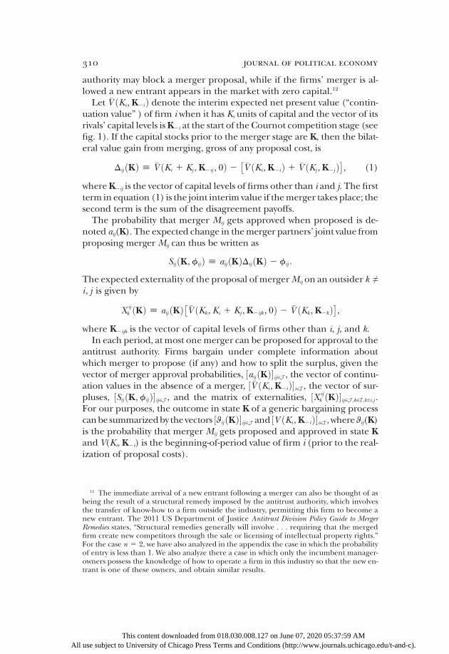
We study a dynamic industry model in which a set of n ≥ 2 firms, I ;f1,… , ng, may invest in capacity, or alternatively merge, to increase theircapital stocks and harness scale economies. The model follows in broadoutline Pakes andMcGuire (1994) and Ericson and Pakes (1995), but withsome important differences in its investment technology, as well as in theintroduction of mergers and merger policy. We focus on symmetric Mar-kov perfect equilibria of our model.Within each period, the sequence of events is as shown in figure 1:
The firms begin each period observing each others’ capital stocks K ;ðK1,… , KnÞ (themodel’s state variable), which affect thefirms’productioncosts. The firms then bargain over which merger, if any, to propose to theantitrust authority. If no merger agreement is reached, the firms proceedto the Cournot competition phase with their current capital levels. If amerger agreement is reached, the merger partners propose their mergerto the antitrust authority, which may then decide to block it. If the mergeris allowed, the firms combine their capital, and a new entrant appears withno initial capital stock. Following thesemerger-bargaining,merger-decision,and entry phases, the active firms engage in Cournot competition giventheir capital stocks, and earn profits on their sales. Following this Cournotcompetition stage, the firms choose their capital investments. Finally, de-preciation may make obsolete some of a firm’s capital. The resulting cap-ital levels after depreciation become the starting values in the next period.We begin by describing the demand and production costs the firms face
(the latter as a function of their capital stocks), and the static Cournot com-petition that occurs in each period.We then detail howmerger bargainingworks, themerger policy of the antitrust authority, and the investment, en-try, and depreciation processes. The appendix contains a more formal de-scription of our model and computational methods.
A. Static Demand, Costs, and Competition
In each period, active firms produce a homogeneous good in a market inwhich the demand function is Q ðpÞ 5 BðA 2 pÞ. The production technol-ogy, which requires capital K and labor L, is described by the productionfunction ðK bLð12bÞÞv, where b ∈ ð0, 1Þ is the capital share and v > 1 the scaleeconomy parameter. Normalizing the price of labor to be 1, for a fixed levelof capital, this production function gives rise to the short-run cost function
This content downloaded from 018.030.008.127 on June 07, 2020 05:37:59 AMAll use subject to University of Chicago Press Terms and Conditions (http://www.journals.uchicago.edu/t-and-c).

FIG.1.—
Sequen
ceofeven
tsin
asingleperiod.
This content downloaded from 018.030.008.127 on June 07, 2020 05:37:59 AMAll use subject to University of Chicago Press Terms and Conditions (http://www.journals.uchicago.edu/t-and-c).

CðQ jK Þ 5 Q 1=½ð12bÞv�
K b=ð12bÞ
with marginal cost
CQ ðQ jK Þ 5 1
ð1 2 bÞv� �
Q 1=½ð12bÞv�f g21
K b=ð12bÞ :
With this technology, amerger that combines the capital of two identicalfirms reduces both average andmarginal cost if their joint output remainsunchanged. This effect will be the source of merger-related efficiencies inour model. Letting R measure the extent of this cost reduction, we have
R ;CQ ð2Q j2K ÞCQ ðQ jK Þ 5
Cð2Q j2K Þ=2QCðQ jK Þ=Q 5 2 1= 12bð Þ½ � 12vð Þ=v½ �:
Note in particular that the marginal cost reduction depends on the scaleeconomyparameter v and capital shareb, but is independent of the outputlevel (and hence demand). In our computations we will focus on a casein which b 5 1=3 and v 5 1:1.9 Given these values, R is .91; that is, amerger of two equal-sized firms results in a 9% efficiency gain.In each period, active firms engage in Cournot competition given their
capital stocks (a firmwith no capital produces nothing), resulting in profitp(Ki,K2i) for a firmwith capital stockKiwhen the vector of its rivals’ capitalstocks is K2i ; ðK1,… , Ki21, Ki11,… , KnÞ.10
internal versus external growth 309
B. Mergers and Bargaining
A mergerMij, which involves the combining of the merging firms’ capital,is feasible between any pair ij ∈ J ; fij ji, j ∈ I , i ≠ jg of firms. Propos-ing merger Mij for approval to the antitrust authority involves a cost fij,which is independent and identically distributed (i.i.d.), both across pairsof firms as well as over time, drawn from a continuous distribution functionFwith support [f, �f].We introduce these proposal costs primarily for tech-nical reasons to ensure existence of (pure strategy) equilibrium; in the realworld, they may represent legal costs.11 As shown in figure 1, the antitrust
9 A capital coefficient of 1/3 is routinely assumed in the macroeconomic literature; see,e.g., Jones (2005). The scale economy parameter of 1.1 is selected so that mergers are stat-ically aggregate surplus increasing in a substantial proportion of industry states.
10 A firm’s short-run cost function is strictly convex if ð1 2 bÞv < 1, in which case there isa unique Cournot equilibrium if the demand function is weakly concave. In our analysis,these conditions are satisfied.
11 See Doraszelski and Satterthwaite (2010) for a discussion of introducing random pri-vate payoffs as a means of ensuring existence.
This content downloaded from 018.030.008.127 on June 07, 2020 05:37:59 AMAll use subject to University of Chicago Press Terms and Conditions (http://www.journals.uchicago.edu/t-and-c).
310 journal of political economy
All
authority may block a merger proposal, while if the firms’ merger is al-lowed a new entrant appears in the market with zero capital.12
Let �V ðKi ,K2iÞ denote the interim expected net present value (“contin-uation value” ) of firm i when it has Ki units of capital and the vector of itsrivals’ capital levels isK2i at the start of the Cournot competition stage (seefig. 1). If the capital stocks prior to the merger stage are K, then the bilat-eral value gain from merging, gross of any proposal cost, is
DijðKÞ ; �V ðKi 1 Kj ,K2ij , 0Þ 2 �V ðKi,K2iÞ 1 �V ðKj , K2jÞ� �
, (1)
whereK2ij is the vector of capital levels of firms other than i and j. The firstterm in equation (1) is the joint interim value if themerger takes place; thesecond term is the sum of the disagreement payoffs.The probability that merger Mij gets approved when proposed is de-
noted aij(K). The expected change in themerger partners’ joint value fromproposing merger Mij can thus be written as
SijðK, fijÞ ; aijðKÞDijðKÞ 2 fij :
The expected externality of the proposal ofmergerMij on an outsider k ≠i, j is given by
Xijk ðKÞ ; aijðKÞ �V ðKk , Ki 1 Kj ,K2ijk , 0Þ 2 �V ðKk ,K2kÞ
� �,
where K2ijk is the vector of capital levels of firms other than i, j, and k.In each period, atmost onemerger can be proposed for approval to the
antitrust authority. Firms bargain under complete information aboutwhich merger to propose (if any) and how to split the surplus, given thevector of merger approval probabilities, ½aijðKÞ�ij∈J , the vector of continu-ation values in the absence of a merger, ½�V ðKi ,K2iÞ�i∈I , the vector of sur-pluses, ½SijðK, fijÞ�ij∈J , and the matrix of externalities, ½X ij
k ðKÞ�ij∈J ,k∈I ,k≠i,j .For our purposes, the outcome in state K of a generic bargaining processcanbe summarizedby thevectors ½ϑijðKÞ�ij∈J and ½V ðKi ,K2iÞ�i∈I , whereϑij(K)is the probability that merger Mij gets proposed and approved in state Kand V(Ki, K2i) is the beginning-of-period value of firm i (prior to the real-ization of proposal costs).
12 The immediate arrival of a new entrant following a merger can also be thought of asbeing the result of a structural remedy imposed by the antitrust authority, which involvesthe transfer of know-how to a firm outside the industry, permitting this firm to become anew entrant. The 2011 US Department of Justice Antitrust Division Policy Guide to MergerRemedies states, “Structural remedies generally will involve . . . requiring that the mergedfirm create new competitors through the sale or licensing of intellectual property rights.”For the case n 5 2, we have also analyzed in the appendix the case in which the probabilityof entry is less than 1. We also analyze there a case in which only the incumbent manager-owners possess the knowledge of how to operate a firm in this industry so that the new en-trant is one of these owners, and obtain similar results.
This content downloaded from 018.030.008.127 on June 07, 2020 05:37:59 AM use subject to University of Chicago Press Terms and Conditions (http://www.journals.uchicago.edu/t-and-c).

internal versus external growth 311
In section III, we focus on the case of two firms (n 5 2) and assumeNash bargaining. In that case, merger M12 gets proposed if and only ifthe bilateral surplus S12(K, f12) is positive. The probability that the mergeroccurs in state K is therefore given by
ϑ12ðKÞ 5 a12ðKÞw12ðKÞ,where w12ðKÞ ; Fða12ðKÞD12ðKÞÞ is the probability of the merger beingproposed. Firm i’s beginning-of-period value in state K includes its possi-ble share of any merger surplus, and equals
V ðKi, K2iÞ 5 �V ðKi , K2iÞ 1 1
2
ð�f
f
S112ðK, f12ÞdFðf12Þ,
where S112ðK, f12Þ ; maxf0, S12ðK, f12Þg. In section IV, we explore situa-
tions with three firms using an adaptation of the bargaining process ofBurguet and Caminal (2015), which we describe there.
C. Merger Policy
The antitrust authority has the ability to block mergers. Blocking a pro-posed merger Mij involves a cost bij ∈ ½b, �b� drawn each period in an i.i.d.fashion fromadistributionH.We introduce these blocking costs primarilyfor technical reasons to ensure existence of (pure strategy) equilibrium;in the real world, they may represent the opportunity costs of an in-depthmerger investigation (which is required for blocking a merger but not forapproving a merger) or possible litigation costs.In our analysis, we focus on a situation in which the antitrust authority
cannot commit to its policy.13 In that case, in any state K, it will decidewhether to block a merger by comparing the increase in its welfare crite-rion from blocking to its blocking cost realization bij. As welfare criteria,we will consider both consumer value (CV) and aggregate value (AV), theexpected net present values of consumer surplus and aggregate surplus,respectively. A Markovian strategy for the antitrust authority is a state-contingent andhistory-independent threshold b̂ijðKÞdescribing thehigh-est blocking cost at which it will block merger Mij in a given state K.Equivalently, this can be translated into a merger acceptance probabilityaijðKÞ ∈ ½0, 1�. As we previously noted, we call the equilibrium policy thatemerges a Markov perfect policy (MPP). In practice, an antitrust author-ity may well lack an ability to commit to its future approval policy. While theDepartment of Justice and Federal Trade Commission in the United Statesperiodically issueHorizontal Merger Guidelines, whichmay partially commit
13 In the appendix, we also consider the case of an antitrust authority that can commit toa deterministic policy ½aijð�Þ�ij∈J that specifies whether a proposed merger would be ap-proved [aijðKÞ 5 1] or not [aijðKÞ 5 0] in each state K.
This content downloaded from 018.030.008.127 on June 07, 2020 05:37:59 AMAll use subject to University of Chicago Press Terms and Conditions (http://www.journals.uchicago.edu/t-and-c).
312 journal of political economy
All
these agencies, over time their actual policy often comes to deviate sub-stantially from the Guidelines’ prescriptions.
D. Investment, Entry, and Depreciation
In Pakes andMcGuire (1994) andEricson andPakes (1995) a firmchoosesin each period how much money to invest, with the probability of success-fully adding 1 unit of capital increasing in the investment level. We departfrom this technology because in a model of mergers it would impose a sig-nificant inefficiency onmergers. In particular, it would restrict the mergedfirm to adding 1 unit of capital each period while, if they had not merged,the firms could have each added 1 unit of capital for a total addition of2 units.14 Instead, we specify an investment technology that ismerger neutralat a market level. By that we mean that a planner who controlled the firmsand wanted to achieve at least cost any fixed increase in themarket’s aggre-gate capital stock would be indifferent about whether the firms merge.With this assumption we isolate the market-level technological effects ofmergers fully in the scale economies of the production function. Thesetechnological effects on production costs, combinedwith firms’ behavioralresponses in investment, will determine the efficiency benefits of mergersin our model.We imagine that there are two ways that a firm can invest. The first is cap-
ital augmentation: each unit j of capital that a firm owns can be doubled atsome cost cj ∈ ½ c, �c � drawn from a distribution F. The draws for differentunits of capital are i.i.d. Thus, for a firm that has K units of capital, thereareK cost draws. Given these draws, if the firm decides to augmentm ≤ Kunits of capital it will do so for the capital units with the cheapest costdraws. Note that capital augmentation is completely merger neutral:when two firms merge, collective investment possibilities do not change.The second is greenfield investment: a firm can build as many capital
units as it wants at a cost cg ∈ ½�c, �cg � drawn from a distribution G. Green-field investment allows a firm whose capital stock is zero to invest, albeitat a cost that exceeds that of capital augmentation. We also choose therange of greenfield costs [�c, �cg] to be small so that this investment tech-nology is approximately merger neutral. (It would be fully merger neu-tral if �cg 5 �c; in our computations we introduce uncertain greenfield in-vestment costs to ensure existence of equilibrium.)As we noted earlier, our model allows for entry. In contrast to Pakes and
McGuire (1994) and Ericson and Pakes (1995), we endow an entrant withthe same investment technology as incumbents. The entrant, however,starts with no capital, so it must use greenfield investment.
14 Alternatively, if the merged firm kept both investment processes we would need tokeep track, as a separate state variable, of how many investment processes a firm possesses,which has no natural bound.
This content downloaded from 018.030.008.127 on June 07, 2020 05:37:59 AM use subject to University of Chicago Press Terms and Conditions (http://www.journals.uchicago.edu/t-and-c).
internal versus external growth 313
Note that with our assumptions investment opportunities will be (ap-proximately)merger neutral at themarket level. The assumptions also im-ply the following two properties of investment costs at the firm level:
1. Holding the firm’s current capital stock K fixed, the expected perunit cost of addingDK units of capital is increasing in the investmentsize DK.15
2. Holding the firm’s investment size DK fixed, the expected invest-ment cost is decreasing in the size of its current capital stock K.16
Both properties are consistent with the large literature on capital adjust-ment costs that Abel (1979) and Hayashi (1982) initiated.17 The secondproperty is also in line with the large (theoretical and empirical) literatureon entry in industrial organization, where it is commonly assumed that po-tential entrants have to incur a setup cost before entering, implying thatnew entrants have to incur higher costs than incumbents if they want toadd the same amount of productive capital.18
Put together, the capital augmentation and greenfield investment pro-cesses allow for significantly richer investment dynamics than in the typicaldynamic industry model. Firms can expand their capital by multiple unitsat a time through either investment method, and new entrants can decideendogenously how far to jump up in their capital stock.Capital also depreciates: in each period each unit of capital has a prob-
ability d > 0 of becoming worthless (including for any future capital aug-mentation).Depreciation realizations are independent across units of cap-ital. This depreciation process is also merger neutral.19 Finally, the firmsdiscount the future according to discount factor d < 1.
15 For a firm with no capital, the unit cost of adding DK units of capital is constant assuch a firm has access to only the greenfield technology.
16 This implies that investment opportunities—while merger neutral at the market level—are not merger neutral at the firm level.
17 Most of the literature on capital adjustment costs assumes that adjustment costs are aconvex function of the proportional change in the firm’s capital stock.With that formulation,the cost of a given sized increase in capital is strictly decreasing in firm size. More recent work,such as Cooper and Haltiwanger (2006), has introduced nonconvex components of adjust-ment costs. But even in those models small firms have very large investment costs.
18 New entrants may also face higher financing costs than established firms. Indeed, thereare many empirical studies finding a positive effect of cash flow on investment, pointing tocredit constraints; see the influential paper by Fazzari, Hubbard, and Petersen (1988) andthe survey by Bond and van Reenen (2007). However, these findings cannot easily bemappedonto ourmodel as cash flow is likely to be related to retained earnings, which in turn dependonownpast capital stocks aswell as rivals’past capital stocks. In the appendix,we also examinethe effects of requiring a minimum scale of greenfield investment.
19 This is in contrast to Ericson and Pakes (1995), Gowrisankaran (1997, 1999), and manyother papers in the computational industrial organization literature. There, depreciation ismodeled as a perfectly correlated industry-wide shock, following which each firm loses 1 unitof capital, independently of its size. That is, these papers assume that the expected deprecia-tion rate is decreasing with firm size.
This content downloaded from 018.030.008.127 on June 07, 2020 05:37:59 AMAll use subject to University of Chicago Press Terms and Conditions (http://www.journals.uchicago.edu/t-and-c).
314 journal of political economy
All
Inour computations firmswill be restricted to an integer number of pos-sible capital levels, with themaximal capital level �K chosen to be nonbind-ing. We define S ; f0, 1, 2,… , �Kg to be the admissible values of Ki andSn 5 S � ⋯� S to be the state space.
III. Merger Policy in Duopoly Markets
In this section we study duopoly markets. While a relatively small share ofmarkets are duopoly markets, and mergers to monopoly are rarely pro-posed and approved, a significant advantage of examining the behaviorof our model in such settings is that the merger bargaining process weadopt for these settings—bilateral Nash bargaining—is well accepted andeasily understood. Throughout most of this section we focus on a singlemarketparameterization so thatwecandescribeequilibriumfirmbehaviorand its interaction with antitrust policy in detail; we discuss afterward howoutcomes vary across a wide range of parameters. We begin in section III.Aby describing the parameters of the market we focus on. In section III.Bwe examine how firms’ behaviors and market performance depend onmerger policy, and in section III.C we study the Markov perfect antitrustpolicy and its positive and normative features. In section III.D we turn tooutcomes for other parameters.
A. Parameterization
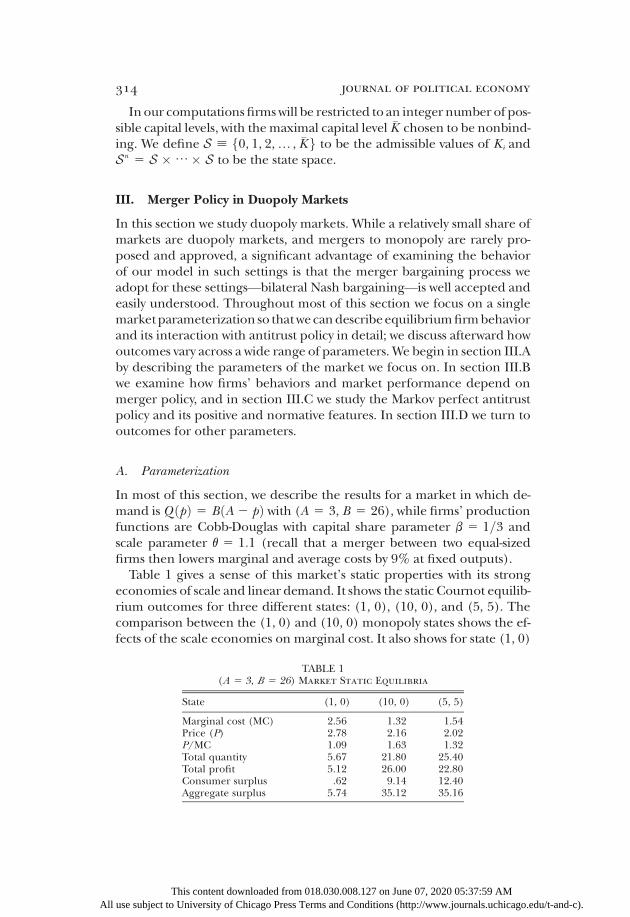
In most of this section, we describe the results for a market in which de-mand is Q ðpÞ 5 BðA 2 pÞ with (A 5 3, B 5 26), while firms’ productionfunctions are Cobb-Douglas with capital share parameter b 5 1=3 andscale parameter v 5 1:1 (recall that a merger between two equal-sizedfirms then lowers marginal and average costs by 9% at fixed outputs).Table 1 gives a sense of this market’s static properties with its strong
economies of scale and linear demand. It shows the static Cournot equilib-rium outcomes for three different states: (1, 0), (10, 0), and (5, 5). Thecomparison between the (1, 0) and (10, 0) monopoly states shows the ef-fects of the scale economies on marginal cost. It also shows for state (1, 0)
Th use subject to U
TABLE 1(A 5 3, B 5 26) Market Static Equilibria
State (1, 0) (10, 0) (5, 5)
Marginal cost (MC) 2.56 1.32 1.54Price (P) 2.78 2.16 2.02P/MC 1.09 1.63 1.32Total quantity 5.67 21.80 25.40Total profit 5.12 26.00 22.80Consumer surplus .62 9.14 12.40Aggregate surplus 5.74 35.12 35.16
is content downloaded from 018niversity of Chicago Press Term
.030.008.127s and Condit
on June 07, 2ions (http://ww
020 05:37:59 AMw.journals.uchicago.edu/t-and-c).

internal versus external growth 315
the effect of linear demandwhen price is high and quantity small: demandis quite elastic causing a small price-cost markup. Aggregate surplus in themonopoly (10, 0) state is almost identical to that in the duopoly (5, 5) statebecause the strong scale economies almost exactly offset the inefficientmonopoly pricing. The distribution of the surplus, however, tilts stronglyaway from consumers and toward producers.Turning to investment costs, the capital augmentation cost for a given
unit of capital is independently drawn from a uniform distribution on[3, 6], while the greenfield investment cost cg is drawn from a uniform dis-tribution on [6, 7].20 Firms’ discount factor is d 5 0:8, corresponding to aperiod length of about 5 years. We chose this to reflect the time to buildnew capital. Each unit of capital depreciates independently with probabil-ity d 5 0:2 per period. We take the state space to be {0, 1, . . . , 20}2, so eachactivefirmcan accumulate up to 20units of capital. In thismarket (and theones considered in section III.D) firms almost never end up outside thequadrant {0, 1, . . . , 10}2; we allow for capital levels up to 20 so that wecan calculate values for mergers and avoid boundary effects. We assumethat proposal and blocking costs are uniformly distributed on [0, 1].21
We focus on these parameter values to highlight the tension betweenthe goals of achieving cost reductions immediately through a merger, pre-venting increased exercise of market power, andmaintaining desirable in-vestment behavior.Finally, as noted at the end of section II, we assume thatmerger bargain-
ing, which occurs between the two active firms, is described by the bilateralNash bargaining solution.
B. Investment and Merger Incentivesunder Fixed Merger Policies
In this section we examine the Markov perfect equilibrium for three typesof fixedmerger policies: (i) the case in whichmergers are prohibited—the“no mergers allowed” case, (ii) the case in which firms are permitted tomerge in any state inwhich it is profitable for them todo so—the “allmerg-ers allowed” case, and (iii) the case of “static”merger policy in whichmerg-ers are blocked if and only if they would result in lower current-period wel-fare. In the third case, we consider both current-period consumer surplusand aggregate surplus as possible welfare measures. For each policy, we
20 The large spread of the capital augmentation cost distribution reflects empirical re-sults showing large variation in firms’ costs within an industry. See, e.g., Bernard et al. (2003)and Syverson (2004). The appendix includes an extension with a smaller variation in firms’costs.
21 We know of no empirical literature on proposal and blocking costs. We chose these widespreads to help ensure convergence of the numerical algorithm. See Doraszelski and Sat-terthwaite (2010).
This content downloaded from 018.030.008.127 on June 07, 2020 05:37:59 AMAll use subject to University of Chicago Press Terms and Conditions (http://www.journals.uchicago.edu/t-and-c).

316 journal of political economy
All
report its long-run steady state distribution over the state spaceS 2, the con-sumer, incumbent, entrant, and aggregate values it generates (the dis-counted expected value of consumer, incumbent, entrant, and aggregatesurpluses, respectively), the investment incentives it creates, and the fre-quency of mergers it induces.
1. Equilibria with No Mergers Allowed
We begin by examining the equilibrium when no mergers are allowed.22
Figure 2A shows the beginning-of-period steady state equilibrium distribu-tion under a no-mergers-allowed policy. (The other panels of fig. 2 showthe steady state distributions for other cases discussed below.) Column 1of table 2 lists some measures of the no-mergers equilibrium.23 As can beseen, under the no-mergers policy the industry spends most of its timein duopoly states in which both firms are active, but also spends roughly18% of the time inmonopoly states. If the industry finds itself in amonop-oly state, it can stay there a long time. For example, figure 3A shows theone-period transition probabilities starting from state (5, 0); it illustratesthe weak entry behavior that allows this monopoly persistence. In fact,starting in state (5, 0), the probability that the industry is a monopoly fiveperiods later is .84.There are two cost-based reasons why it is so hard for an entrant starting
in state (5, 0) to catch up. First, the entrant pays much more per unit ofcapital purchased: the large firm can add a unit of capital using the lowestof its five cost draws from the uniform distribution on [3, 6], whereas theentrant draws from the uniform distribution on [6, 7]. Second, the largefirm’s scale economies give it a marginal cost of 1.70 when setting a mo-nopoly price of 2.35. If the potential entrant should enter with 2 units ofcapital, then at state (5, 2) the dominant firm sells quantity 14.6 at a priceof 2.18 with marginal cost 1.62. The entering firm sells 6.7 units with mar-ginal cost 1.92. Profits are 14.5 and 5.1, respectively.
2. Equilibria with All Mergers Allowed
Under an all-mergers-allowed policy, equilibrium is quite different. Fig-ure 2B shows the beginning-of-period steady state equilibrium distribu-tion under an all-mergers-allowed policy, as well as the probability that a
22 We have assembled the data that we have generated into large Excel workbooks thateach contain for each equilibrium, first, a detailed description of the equilibrium strategiesof the firms and, for Markov perfect merger policies, of the antitrust authority, and second,a full set of performance statistics. These workbooks are provided as supplementary mate-rial online. They enable the reader to explore our results much as we have explored them.
23 For comparison, in the first-best solution (with price equal to marginal cost and aggre-gate value-maximizing investment), the aggregate value is 164.7 and the average total cap-ital level is 10.6.
This content downloaded from 018.030.008.127 on June 07, 2020 05:37:59 AM use subject to University of Chicago Press Terms and Conditions (http://www.journals.uchicago.edu/t-and-c).
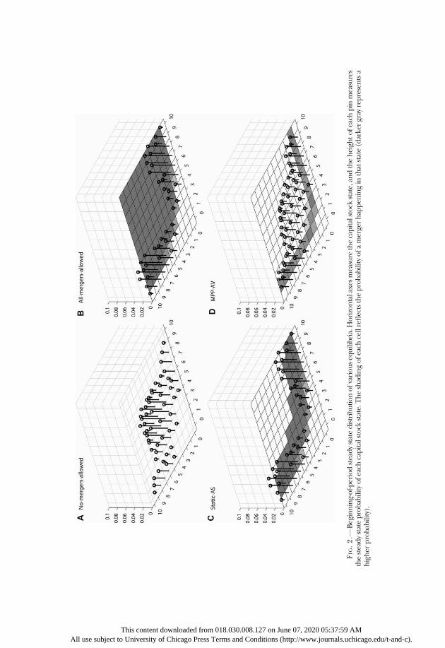
FIG.2.—
Beginning-of-p
eriodsteadystatedistributionofvariousequilibria.Horizontalaxesmeasure
thecapitalstock
state,an
dtheheigh
tofeachpin
measures
thesteadystateprobabilityofeachcapitalstock
state.Theshadingofeachcellreflectstheprobabilityofa
mergerhappen
ingin
thatstate(darkergray
representsa
higher
probability).
This content downloaded from 018.030.008.127 on June 07, 2020 05:37:59 AMAll use subject to University of Chicago Press Terms and Conditions (http://www.journals.uchicago.edu/t-and-c).

318 journal of political economy
All
merger actually happens in each state. Shading shows states inwhichmerg-ers occur with a darker shade representing a higher probability of amergerhappening; cells inwhichmergers never occur are unshaded: for example,a merger happens with probability 1 in state (3, 3), with probability zero instate (2, 2), and with probability .59 in state (2, 3). Observe that firms donot always merge in nonmonopoly states. The reason is that if both firms’capital stocks are low, then merging attracts a new entrant that dissipatesthe merger’s gains.Column 2 of table 2 shows the properties of the all-mergers-allowed
equilibrium.Mergers happen 37.7% of the time, which results in themar-ket being in amonopoly state (at the time of Cournot competition) 86.0%of the time, and in a near-monopoly state 99.1% of the time. As a result ofallowingmergers, average output falls from 22.2 to 19.2, while the averageprice rises from 2.15 to 2.26. Average total capital falls from 8.0 to 7.0. Notsurprisingly, the change in policy leads to substantial negative changes inconsumer value, which falls from 48.1 to 35.8. More surprisingly, averageincumbent value falls even though the firms are now allowed to mergewhenever they want. This is despite firms’ success in raising price, reduc-ing quantity, and limiting total capital. Even once one accounts for future
TABLE 2Performance Measures for the (A 5 3, B 5 26)
Market under Various Policies
Performance Measure
No Mergers/Static CS/MPP CV All Mergers Static AS MPP AV
(1) (2) (3) (4)
Average consumer value 48.1 35.8 35.9 43.3Average incumbent value 69.4 68.1 68.5 69.9Average entrant value 0 1.9 1.8 .5Average blocking cost 0 0 0 2.1Average aggregate value 117.5 105.8 106.2 113.6Average price 2.15 2.26 2.26 2.19Average quantity 22.2 19.2 19.2 21.0Average total capital 8.0 7.0 7.0 7.7Merger frequency (%) 0 37.7 37.9 16.1Percentage in monopoly 18.6 86.0 88.0 49.4Percentage ofmin{K1, K2} ≥ 2 75.7 .9 .7 44.2
State (0, 0) CV 30.3 23.9 24.1 25.6State (0, 0) AV 36.7 34.0 34.1 35.5
This content dow use subject to University of Ch
nloaded from 018.030.008.1icago Press Terms and Cond
27 on June 07, 2itions (http://ww
020 05:37:59w.journals.u
Note.—All values are ex ante (beginning ofperiod) values except percentage inmonopolyand minfK1, K2g ≥ 2 (showing the percentages of the time that industry capital is in eachtype of state), which are at the Cournot competition stage. “No Mergers” and “All Mergers”refer to the no-mergers-allowed and all-mergers-allowed policies, respectively. “Static CS”and “Static AS” refer, respectively, to the equilibria under the optimal static consumer-surplus-based and aggregate-surplus-based merger policies. “MPP CV” and “MPP AV” refer, respec-tively, to the equilibria when the antitrust authority cannot commit (resulting in a Markovperfect policy) under consumer value and aggregate value welfare criteria. “State (0,0) CV”and “State (0,0) AV” are the values of CV and AV, respectively, for a new industry that startswith no capital.
AMchicago.edu/t-and-c).

FIG. 3.—One-period transition probabilities from state (5, 0). Horizontal axes measurethe capital stock state, and the height of each pin measures the transition probability fromstate (5, 0).
This content downloaded from 018.030.008.127 on June 07, 2020 05:37:59 AMAll use subject to University of Chicago Press Terms and Conditions (http://www.journals.uchicago.edu/t-and-c).

320 journal of political economy
All
entrants’ value, producer value (the sum of incumbent and entrant val-ues) barely rises. Combinedwith the reduction inCV, aggregate value fallsfrom 117.5 to 105.8.To explore the reasons behind these results, consider first the reduction
in total capital. Allowing mergers does two things. First, it changes thestates in which investments are taking place by moving the market to mo-nopoly and near-monopoly states. Second, firms’ investment policieschange. Table 3 summarizes these effects. Holding investment behaviorfixed, average capital addition decreases when weighted by the all-mergers-allowedsteadystateratherthantheno-mergers steadystate.However,hold-ing the steady stateweightingfixed, average capital addition increases wheninvestment behavior is that of the all-mergers-allowed equilibrium ratherthan the no-mergers equilibrium. Together, these opposite effects reducethe average capital addition moving from the no-mergers-allowed policyto all mergers allowed.What drives the increased investment incentive? If amerger is certain to
occur next period, a firm i’s marginal return to investment is ∂�V ðKi, KjÞ=∂Ki 1 ð1=2Þ∂DijðKi, KjÞ=∂Ki , where ∂DijðKi, KjÞ=∂Ki is the marginal effectof Ki on the gain from merger as defined in equation(1).24 Each firm isin a state where ∂DijðKi, KjÞ=∂Ki is positive 97.5% of the time in the no-mergers steady state and 100%of the time in the all-mergers-allowed steadystate; the fact that a firm’s gains from a merger are increasing in its capitalstock tends to make allowing mergers increase investment incentives.25
In the all-mergers-allowed equilibrium the steady state distribution isconcentrated in monopoly and near-monopoly states. The increased in-vestment incentive is particularly large and detrimental to producer valuein such states. An entrant with zero capital frequently invests in the hopeofbeing bought out: there is a great deal of “entry for buyout” behavior(Rasmusen 1988).26 For example, figure 3B shows the one-period transi-tion probabilities in state (5, 0) when all mergers are allowed, which canbe compared to figure 3A, where nomergers are allowed. The probabilitythat the entrant invests and has nonzero capital after depreciation is .57in the former case, versus .04 in the latter. Further, the probability of amerger is .49 in the first period after the entrant invests when all mergers
24 This abstracts away from the discrete nature of capital additions.25 The change from the no-mergers-allowed to the all-mergers-allowed policy also changes
the interim value function �V ð�Þ.26 While we are unaware of any formal empirical studies that document the frequency of
entry-for-buyout behavior, Rasmusen (1988) gives a number of examples of entry for buy-out in homogeneous-goods industries. In the literature on start-ups, acquisition is consid-ered to be one of the primary ways of capturing a start-up’s value (see, e.g., Gans and Stern2003). Although start-ups frequently introduce product innovations and do not literally fitour homogeneous-goods model, we can reinterpret the capital in our model as “knowledgecapital” and the resulting cost reductions are enabled to be consumer value enhancementsthat increase the firm’s profit.
This content downloaded from 018.030.008.127 on June 07, 2020 05:37:59 AM use subject to University of Chicago Press Terms and Conditions (http://www.journals.uchicago.edu/t-and-c).

internal versus external growth 321
are allowed, and .85 within two periods. Figure 3B also shows that the en-trant’s increased investment lowers the incentive of the incumbent to in-vest in state (5, 0).This entry-for-buyout behavior reduces producer value as the entrants’
investments are made at high cost and displace lower cost investments bythe incumbent monopolist. Figure 4 illustrates the destructiveness of thisbehavior for producer value. It shows for each state the change in the rowfirm’s (firm 1) beginning-of-period value that a switch from a no-mergers-allowed to an all-mergers-allowed policy induces. In most states the rowfirm’s value is enhanced but in monopoly states in which the monopolisthas at least 3 units of capital, themonopolist’s value falls dramatically. Thisbehavior is also highly detrimental for aggregate value: In both the no-mergers and all-mergers-allowed equilibria, dominant firms generallyhave insufficient incentives, while entrants have excessive incentives.27
The entry-for-buyout phenomenon therefore causes a shift in investmentaway from thedominant firm, whose incentives are already insufficient, to-ward the entrant, whose incentives are excessive.
3. Equilibria with Static Policies
We next consider optimal static merger policy, as in Williamson (1968)and Farrell and Shapiro (1990). These policies block a merger if and onlyif it decreases welfare (either consumer surplus or aggregate surplus, de-pending on the criterion) due to production and consumption in the pe-riod in which the merger occurs.28
Mergers lower consumer surplus in all but state (1, 1), so the staticconsumer-surplus-based policy is essentially equivalent to allowing nomergers.In contrast, figure 5 shows that many mergers increase aggregate sur-
plus. In general, these tend to be states in which the total capital in the in-dustry is not more than 10, though in some asymmetric states with total
27 Thecentives
28 Anoner contput decimerger
All use s
TABLE 3Average Capital Addition in the (A 5 3, B 5 26) Market
Investment Behavior
Steady State Distribution
No Mergers All Mergers Allowed
No mergers 2.0 1.5All mergers allowed 2.2 1.8
appendix contains tables showand the benefits to social welfarther possible benchmark is therols firms’merger decisions as wesions. This benchmark is analyzpolicy is very similar to the optim
This content downloaded frubject to University of Chicago Pre
ing the difference be from investment.second-best dynamill as their investmened in the appendixal static aggregate-
om 018.030.008.127ss Terms and Conditi
etween firms’ investment in-
c problem in which the plan-t decisions, but not their out-
. It turns out this second-bestsurplus-based policy.
on June 07, 2020 05:37:59 AMons (http://www.journals.uchicago.edu/t-and-c).

322 journal of political economy
All
capital above 10 there is also a gain.29 The gains in aggregate surplus aregenerally smaller the larger the total capital in the industry.30 An increasein the asymmetry of capital positions, holding total capital fixed, has vary-ing effects on the static gains in aggregate surplus fromamerger. This gaingets smaller with increased asymmetry at low levels of total capital, butgrows larger with increased asymmetry at greater levels of total capital.Figure 2C shows the beginning-of-period steady state equilibrium distri-
bution under the aggregate-surplus-based static merger policy and table 2shows equilibrium performance statistics under this policy. As can be seenin the figure and table, the outcomewith the aggregate-surplus-based staticpolicy is very close to the all-mergers-allowed outcome.
C. Equilibria with Markov Perfect Merger Policy
We now introduce an optimizing antitrust authority that cannot committo its future policy, determine its Markov perfect policy, and examine
FIG. 4.—Beginning-of-period value of the row firm (firm 1) in the all-mergers-allowed equi-librium minus its value in the no-mergers equilibrium. Negative numbers are in parentheses.
29 The only exception is state (5, 5), in which the static gain in aggregate surplus is ap-proximately zero.
30 To understand this result, observe that the change in aggregate surplus from amergerin a symmetric state is approximately
QDQ
Q
� �ðP 2 MCÞ 2 1 1
DQ
Q
� �DACM
ACM
� �ACM
� �,
where P 2 MC is the premerger price-cost margin, ACM is the average cost if no mergeroccurs but the output level changes to its postmerger level, and DACM is the change in av-erage cost at the postmerger output level due to the combination of capital. At larger cap-ital levels, P 2 MC and FDQ=QF are both greater, DACM=ACM is unchanged, and ACM issmaller, making the sign of the effect on aggregate surplus more likely to be negativefor an output-reducing merger. For example, P 2 MC is 0.32 at state (2, 2) and 0.45 at state(4, 4), DQ=Q is20.065 at (2, 2) and20.126 at (4, 4), and ACM is 21% lower at (4, 4) than at(2, 2).
This content downloaded from 018.030.008.127 on June 07, 2020 05:37:59 AM use subject to University of Chicago Press Terms and Conditions (http://www.journals.uchicago.edu/t-and-c).

internal versus external growth 323
the outcome it induces. In this setting the antitrust authority, like each ofthe firms, is a player in a dynamic stochastic game; Markov perfection re-quires that in each state the policy survive the one-stage-deviation test.31
As with the static consumer-surplus-based policy, the Markov perfectpolicy outcome when the antitrust authority seeks to maximize consumervalue (CV) is essentially equivalent to the no-mergers-allowed outcome(see table 2). For the rest of this section, we therefore focus on an authoritythat seeks to maximize aggregate value (AV).For an antitrust authority following the AV criterion, neither the no-
mergers-allowed nor the all-mergers-allowed policy survives the one-stage-deviation test given the firm behavior it induces: assuming future behaviorfollowing the no-mergers equilibrium, the antitrust authority would allowmanymergers in a one-stage deviation; assuming future behavior followingthe all-mergers-allowed equilibrium, the antitrust authority would allowvery few mergers.Figure 2D’s shading shows the probability that amerger occurs in various
states under theMarkov perfect policy. The policy differs markedly from allof the policies we have previously considered. The authority approves a pro-posed merger with positive probability in near-monopoly states in whichminfK1, K2g 5 1, as well as in states (2, 2), (3, 2), and (2, 3). Given this pol-icy,mergers are proposedwith probability 1 in all these states, except in state(1, 1), where a merger is never proposed, and in states (2, 1) and (1, 2),where amerger is proposedwith less than full probability. This policy inducesan even higher merger probability following entry than the all-mergers-allowed policy: For example, the probability of a merger is .69 in the first
FIG. 5.—Static change in aggregate surplus from a merger in the (A 5 3, B 5 26) mar-ket. Negative numbers are in parentheses.
31 In the appendix we discuss as well the case in which the antitrust authority can committo its future policy.
This content downloaded from 018.030.008.127 on June 07, 2020 05:37:59 AMAll use subject to University of Chicago Press Terms and Conditions (http://www.journals.uchicago.edu/t-and-c).

324 journal of political economy
All
period after entry in state (5, 0), compared to .49 in the all-mergers-allowedequilibrium. Firms are more likely to merge in the first period under theMarkov perfect policy because if the entrant grows further they are unlikelyto be allowed to merge in the second period.Figure 2D also shows the steady state distribution arising under theMar-
kov perfect policy, while table 2 shows its performance statistics. The indus-try is in a monopoly state at the Cournot competition stage 49.4% of thetime, and in near-monopoly states 55.8% of the time. Compared to thesteady state induced when no mergers are allowed, the economy spendsmuch more time in such states. In addition, the average aggregate capitallevel is lower (7.7 vs. 8.0). The reason is the shift in the steady state distri-bution toward more asymmetric states, in which investments are lower.However, because a new entrant and the incumbent are not always allowedto merge, monopoly states are less frequent and average capital is greaterthan under the all-mergers-allowed and static aggregate-surplus-basedpolicies.The Markov perfect policy with the AV criterion is much better for con-
sumers and aggregate value than allowing all mergers or following thestatic aggregate-surplus-based policy. However, it results in a level of steadystate AV that is about 3% lower than with the no-mergers policy: AV is113.6 compared to 117.5 when no mergers are allowed.32 Firms are onlyslightly better off—harmed again by the entry-for-buyout behavior themerger policy induces—while consumers are much worse off: CV is 43.3(vs. 48.1) and producer value is 70.4 (vs. 69.4). Consumers are harmedfrom both the monopoly pricing and the reduction in capital. Strikingly,observe that a commitment to maximizing CV or to the static consumer-surplus-based policy would be better here for aggregate value than the pol-icy that results when the antitrust authority seeks to maximize AV but can-not commit.33
D. Results for Other Demand Parameters
Up to this point we have limited our discussion to a single market param-eterization. While this focus allowed us to discuss in detail the outcomesand strategies that arise in this case, it naturally leaves open the questionof how our results extend to other market conditions. Here we examine
32 The finding that the Markov perfect policy with the AV criterion performs worse thanthe no-mergers policy but better than the all-mergers-allowed policy holds not only for thesteady state averages of AV and CV but also for a “new” industry: as shown in table 2, at state(0, 0) the AV (resp. CV) value of the Markov perfect policy is 35.5 (25.6), that of the no-mergers policy 36.7 (30.3), while that of the all-mergers-allowed policy is only 34.0 (23.9).
33 This conclusion is reminiscent of Lyons (2002), but arises for different reasons.
This content downloaded from 018.030.008.127 on June 07, 2020 05:37:59 AM use subject to University of Chicago Press Terms and Conditions (http://www.journals.uchicago.edu/t-and-c).

internal versus external growth 325
the extent to which several of the features of the equilibria discussed ex-tend across a wider range of demand parameters.34
We first examine how the no-mergers-allowed and all-mergers-allowedequilibria differ. Figure 6A reports on the difference in aggregate value be-tween these two policies for linear demand functions Q ðpÞ 5 BðA 2 pÞ,whereA is the chokeprice andB is themarket size parameter (e.g., numberof consumers). The figure depicts contour lines showing the demand pa-rameters at which the aggregate value difference, ðAVNo 2 AVAllÞ=AVNo,achieves a given percentage value. Also shown in the figure are three dots.The middle one is the (A 5 3, B 5 26) market that our discussion abovefocused on. The other two dots represent a “smaller” and a “larger”marketwhose equilibria we discuss in greater detail in the appendix, parallelingour discussion above of the (A 5 3, B 5 26)market. In the figure, dashedlines showmarkets that spend 5%, 20%, and 60% of the time inmonopolystates when nomergers are allowed. Market parameters to the upper rightin thefigure are largemarketswith low levels ofmonopoly, whilemarkets tothe lower left are small markets with high monopoly levels. As can be seenin the figure, aggregate value with nomergers allowed is greater than withall mergers allowed provided that the market is large enough, with aggre-gate value approximately equal for these twomerger policies formarkets inwhich the no-mergers-allowed equilibrium spends about 70% of the timein monopoly states.For the same range of demandparameters, figure 6B shows the percent-
age difference in entry probabilities in the no-mergers-allowed and all-mergers-allowed equilibria, ½Pr ðEntryÞAll 2 Pr ðEntryÞNo�= Pr ðEntryÞAll.35Consistent with the entry for buyout we observed earlier, the level of entryis always weakly greater in the all-mergers-allowed equilibrium, althoughthe difference declines to zero in very large markets where the probabilityof entry rises to 1 under either merger policy.
34 In the appendix we also consider the effect of varying the production scale parameterv. The results show similar patterns to those we discuss here, with outcomes closely relatedto the percentage of time spent in monopoly states when no mergers are allowed. We alsoexamine there the following modeling extensions: allowing the probability of entry follow-ing a merger to be less than 1; modifying our greenfield investment technology (used pri-marily by entrants) to require a minimum scale of investment greater than 1 unit of capital;reducing the gap of investment costs faced by incumbents and entrants; having bargainingpower proportional to capital stocks; allowing a planner to control investment behaviorand merger decisions taking as given only Cournot competition; and assuming new en-trants are the owners of the firms purchased in mergers.
35 Pr(Entry)x is calculated by weighting the probability of entry in eachmonopoly state un-der merger policy x by the probability of that state in the all-mergers-allowed equilibrium. Inthe lower right region of the figure, the no-mergers equilibrium has no entry in states thatarise with positive probability in the all-mergers-allowed equilibrium, leading the percentagedifference in entry probabilities to be 100%.
This content downloaded from 018.030.008.127 on June 07, 2020 05:37:59 AMAll use subject to University of Chicago Press Terms and Conditions (http://www.journals.uchicago.edu/t-and-c).

All
FIG. 6.—A, Contour lines of the percentage difference between the steady state aggre-gate value of the no-mergers and all-mergers-allowed equilibria, ðAVNo 2 AVAllÞ=AVNo.B, Contour lines of the percentage difference between the entry probabilities of the no-mergers and all-mergers-allowed equilibria, ½Pr ðEntryÞAll 2 Pr ðEntryÞNo�= Pr ðEntryÞAll�.In both panels A and B, the dashed lines show markets that spend 5%, 20%, and 60%of the time in monopoly states when no mergers are allowed.
This content downloaded from 018.030.008.127 on June 07, 2020 05:37:59 AM use subject to University of Chicago Press Terms and Conditions (http://www.journals.uchicago.edu/t-and-c).

internal versus external growth 327
Figure 7 focuses on theMarkov perfect policy. Figure 7A shows the per-centage difference in aggregate value between the Markov perfect policyand the no-mergers-allowed equilibria, ðAVMPP 2 AVNoÞ=AVMPP. Insmall markets, the Markov perfect policy leads to higher aggregate valuethan when no mergers are allowed. Similarly to the comparison betweenthe no-mergers and all-mergers-allowed policies, the no-mergers policyoutperforms the Markov perfect policy provided the market is largeenough. However, for the largest markets in the upper right corner, theMarkov perfect policy leads to the same equilibriumas the no-mergers pol-icy becausemergers are never consummated. Figure 7B shows the sameAVcomparison but relative to the outcome with the static aggregate-surplus-based policy, ðAVMPP 2 AVStaticÞ=AVMPP. The figure shows that the Markovperfect policy outperforms the static aggregate-surplus-based policy pro-vided the market is large enough.
IV. Merger Policy in Triopoly Markets
In this section, we extend our framework by introducing a third firm. Thekey novelty in the triopoly case is that a bilateralmergermay now induce anexternality on the nonmerging firm, which in turn introduces some newinvestment incentives not present in our earlier duopoly markets. Ouranalysis here should be viewed as giving a glimpse of the new effects thiscan introduce, as we do this for one particular three-party bargaining pro-cess amongmany possible ones. Triopolymarkets also allow us to study op-timal policy toward mergers that combine two weaker (i.e., lower capitalstock) firms that face a stronger rival, an issue that arises frequently inmerger cases (such as the AT&T/T-Mobile USA and Sprint/T-Mobile USAmergers).We first examine the robustness of our previous two-firm results to the
possibility of a third firm. We show that the (A 5 3, B 5 26) market thatwe studied in section III is a “natural duopoly” in the sense that a third firmdoes not wish to enter when nomergers are allowed, although whenmerg-ers are allowed the entry-for-buyout motive sometimes leads a third firmto enter temporarily. Nonetheless, our previous conclusions continue tohold. We then examine merger policy in two “natural triopoly” markets,wherewhennomergers are allowed themarket usually has three firmswithpositive levels of capital. The presence of externalities on nonmergingfirms introduces a new effect on incumbent investment that impacts opti-mal merger policy significantly in one of these markets.To proceed, we consider a three-firm version of the general model of
section II. The bargaining stage in each period is a static version of the bar-gaining protocol in Burguet and Caminal (2015): One firm, say i, is ran-domly selected as the proposer, with each firm equally likely to be selected.
This content downloaded from 018.030.008.127 on June 07, 2020 05:37:59 AMAll use subject to University of Chicago Press Terms and Conditions (http://www.journals.uchicago.edu/t-and-c).

All
FIG. 7.—A, Contour lines of the percentage difference between the steady state aggre-gate value of the MPP-AV and no-mergers equilibria, ðAVMPP 2 AVNoÞ=AVMPP. B, Contourlines of the percentage difference between the steady state aggregate value of the MPP-AVand static aggregate-surplus-based policy equilibria, ðAVMPP 2 AVStaticÞ=AVMPP. In both pan-els A and B, the dashed lines show markets that spend 5%, 20%, and 60% of the time inmonopoly states when no mergers are allowed.
This content downloaded from 018.030.008.127 on June 07, 2020 05:37:59 AM use subject to University of Chicago Press Terms and Conditions (http://www.journals.uchicago.edu/t-and-c).
internal versus external growth 329
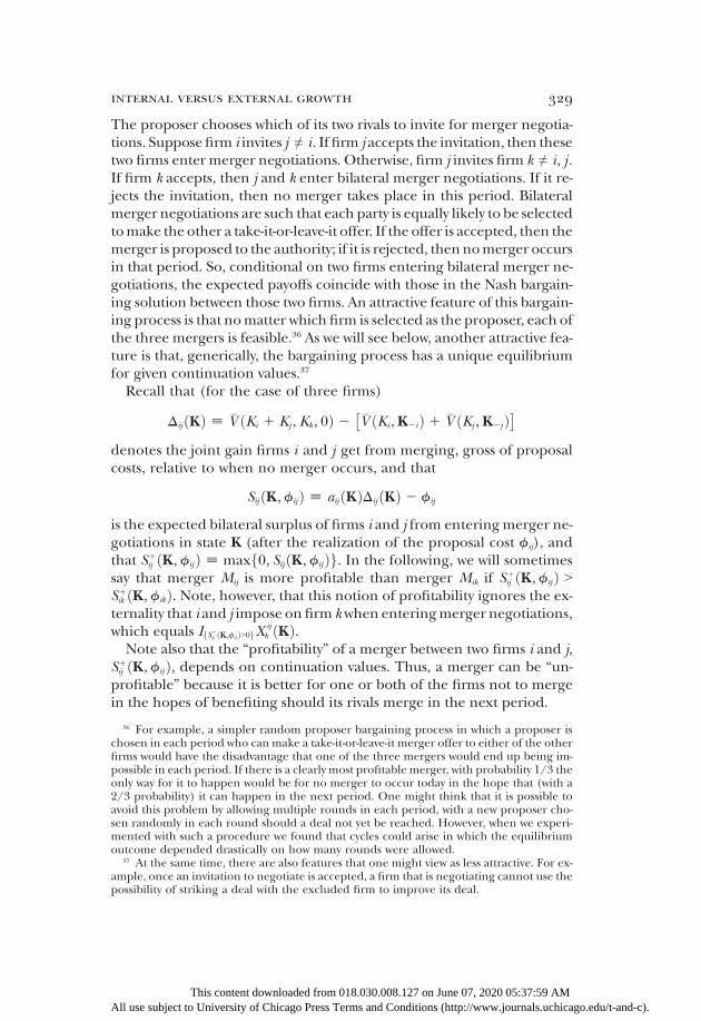
The proposer chooses which of its two rivals to invite for merger negotia-tions. Supposefirm i invites j ≠ i. If firm j accepts the invitation, then thesetwo firms enter merger negotiations. Otherwise, firm j invites firm k ≠ i, j .If firm k accepts, then j and k enter bilateral merger negotiations. If it re-jects the invitation, then no merger takes place in this period. Bilateralmerger negotiations are such that each party is equally likely to be selectedtomake the other a take-it-or-leave-it offer. If the offer is accepted, then themerger is proposed to the authority; if it is rejected, thennomerger occursin that period. So, conditional on two firms entering bilateral merger ne-gotiations, the expected payoffs coincide with those in the Nash bargain-ing solution between those two firms. An attractive feature of this bargain-ing process is that nomatter which firm is selected as the proposer, each ofthe three mergers is feasible.36 As we will see below, another attractive fea-ture is that, generically, the bargaining process has a unique equilibriumfor given continuation values.37
Recall that (for the case of three firms)
DijðKÞ ; �V ðKi 1 Kj , Kk , 0Þ 2 �V ðKi ,K2iÞ 1 �V ðKj ,K2jÞ� �
denotes the joint gain firms i and j get from merging, gross of proposalcosts, relative to when no merger occurs, and that
SijðK, fijÞ ; aijðKÞDijðKÞ 2 fij
is the expected bilateral surplus of firms i and j from entering merger ne-gotiations in state K (after the realization of the proposal cost fij), andthat S1
ij ðK, fijÞ ; maxf0, SijðK, fijÞg. In the following, we will sometimessay that merger Mij is more profitable than merger Mik if S1
ij ðK, fijÞ >S1ik ðK, fikÞ. Note, however, that this notion of profitability ignores the ex-ternality that i and j impose on firm kwhen enteringmerger negotiations,which equals IfS1
ij ðK,fij Þ>0gXijk ðKÞ.
Note also that the “profitability” of a merger between two firms i and j,S1ij ðK, fijÞ, depends on continuation values. Thus, a merger can be “un-profitable” because it is better for one or both of the firms not to mergein the hopes of benefiting should its rivals merge in the next period.
36 For example, a simpler random proposer bargaining process in which a proposer ischosen in each period who can make a take-it-or-leave-it merger offer to either of the otherfirms would have the disadvantage that one of the three mergers would end up being im-possible in each period. If there is a clearly most profitable merger, with probability 1/3 theonly way for it to happen would be for no merger to occur today in the hope that (with a2/3 probability) it can happen in the next period. One might think that it is possible toavoid this problem by allowing multiple rounds in each period, with a new proposer cho-sen randomly in each round should a deal not yet be reached. However, when we experi-mented with such a procedure we found that cycles could arise in which the equilibriumoutcome depended drastically on how many rounds were allowed.
37 At the same time, there are also features that one might view as less attractive. For ex-ample, once an invitation to negotiate is accepted, a firm that is negotiating cannot use thepossibility of striking a deal with the excluded firm to improve its deal.
This content downloaded from 018.030.008.127 on June 07, 2020 05:37:59 AMAll use subject to University of Chicago Press Terms and Conditions (http://www.journals.uchicago.edu/t-and-c).

330 journal of political economy
All
The following proposition completely characterizes the equilibriumoutcome of the merger process.Proposition 1. Suppose firm i is selected as the proposer in state K.
Then the following hold:
i. If S1jk ðK, fjkÞ > maxfS1
ij ðK, fijÞ, S1ik ðK, fikÞg, then firm i invites either
firm j or firm k, and merger Mjk gets proposed.ii. If S1
ij ðK, fijÞ > S1ik ðK, fikÞ ≥ S1
jk ðK, fjkÞ, then firm i invites firm j , andmerger Mij gets proposed.
iii. If S1ij ðK, fijÞ > S1
jk ðK, fjkÞ > S1ik ðK, fikÞ and S1
ij ðK, fijÞ=2 > Xjki ðKÞ,
then firm i invites firm j, and merger Mij gets proposed.iv. If S1
ij ðK, fijÞ > S1jk ðK, fjkÞ > S1
ik ðK, fikÞ and S1ij ðK, fijÞ=2 < X
jki ðKÞ,
then firm i invites firm k, and merger Mjk gets proposed.v. If S1
ij ðK, fijÞ 5 S1jk ðK, fjkÞ 5 S1
ik ðK, fikÞ 5 0, thennomergeroccurs.
In case i, even though firm i is the proposer, mergerMjkmust be the out-come as both firms j and k prefer their half of the surplus frommergerMjk,S1jk ðK, fjkÞ, to what they can get bargaining with firm i. In contrast, in case ii,both j and k prefer to split the bargaining surplus available in a deal withfirm i to bargaining with each other. So firm i can get either mergerMij ormergerMik, andprefers the former. In cases iii and iv, firm i will getmergerMij if it proposes bargainingwith firm j ( jprefers to split surplus withfirm irather than with firm k), but can induce the second-most profitablemergerMjkby proposing tobargainwithfirm k (kprefers to bargainwith j); whichofthese options firm i prefers depends on comparing its split of the bargain-ing surplus with firm j to the externality it experiences when merger Mjk
happens. In case v, nomerger has a positive surplus, so nomerger occurs.38
A formal proof is in the appendix. Observe that mergerMjk will happen intwo circumstances when firm i is the proposer: whenMjk is the most profit-ablemerger, andwhenMjk ismoreprofitable thanMik and firm i gainsmorewhen merger Mjk occurs than its half of merger Mij’s surplus.
A. Allowing a Third Firm in the ðA 5 3, B 5 26Þ Market
When no mergers are allowed in the (A 5 3, B 5 26) market, introduc-ing a third firm has almost no impact as triopoly states are very rare: stateswith three active firms are visited only about 0.5% of the time. That is, thetwo-firm equilibrium outcome we studied in section III when no mergers
38 We assume that firms i and j do not merge if aijðKÞDijðKÞ 2 fij 5 0; however, in case vthis is a measure-zero event: generically we have aijðKÞDijðKÞ 2 fij < 0 for all i and j. Noteas well that since the surplus measures the bilateral gain from a merger relative to nomerger occurring, one reason that a merger may have negative surplus is that one or bothfirms anticipate the possibility of experiencing a positive externality should rivals merge ina subsequent period.
This content downloaded from 018.030.008.127 on June 07, 2020 05:37:59 AM use subject to University of Chicago Press Terms and Conditions (http://www.journals.uchicago.edu/t-and-c).
internal versus external growth 331
are allowed approximates well the outcome of a “free entry” equilibrium.(Equilibrium statistics when we allow a third firm are displayed in the ap-pendix.) In this sense, it is a “natural duopoly” market.39
When mergers are allowed, however, the prospect of entry for buyoutcan lead both a second and a third firm to enter for the prospect of beingacquired.40 When this happens a subsequent merger induces a duopolyrather than a monopoly outcome. As a result, introducing the possibilityof a third active firm reduces the steady state frequency of a monopolystate from 86.0% to 85.4%, but increases the probability of a merger from37.7% to 50.8%.41
Despite these quantitative changes in the equilibrium outcome, ourprevious insights carry over to the three-firm case. Allowing all mergers in-duces entry for buyout and implies that the industry spends much moretime in amonopoly state: the steady state frequency ofmonopoly increasesfrom 18.0% under the no-mergers policy to 85.4% under the all-mergers-allowed policy. Since firms invest on average less in such monopoly statesthan inmore symmetric states, the average total capital level is lower underthe all-mergers-allowed policy.42 Because the industry spendsmore time inmonopoly and firms invest less, consumers are much worse off when allmergers are allowed: consumer value decreases from 48.3 to 38.0. Despitethe large increase in the frequency of monopoly, firms collectively do notgain much from allowing all mergers because of the distortions in firms’investment behavior associated with entry for buyout. As a result, averageAV falls from 117.6 to 107.7 when all mergers are allowed.Turning to theMarkov perfect policy, when the authority uses theAV cri-
terion the steady state probability that the industry finds itself in a duopolystate before merger is high (77.6%), and the likelihood of triopoly is low(2.2%). In duopoly states, the antitrust authority approves a merger onlywhen at least one of the incumbents is very small, and is more restrictivethan would be statically optimal; a merger happens 13.3% of the time
39 The same is true in the “small” (A 5 3, B 5 22) and “large” (A 5 3, B 5 30) marketsdiscussed in the appendix.
40 For example, with two firms the probability that the entrant invests in state (5, 0) was58%. With three firms, in state (5, 0, 0), the probability that each entrant invests is onlyslightly smaller, namely 51%. This implies that, starting from state (5, 0, 0), the probabilitythat there are three firms with capital at next period’s merger stage is equal to 16.7% (theprobability that both entrants invest times the probability that neither entrant’s capital de-preciates). At the same time, the probability that no entry (and therefore no merger) oc-curs in state (5, 0, 0) is considerably lower than in state (5, 0), namely, 35.0% rather than53.6%. Note, however, that our restriction to symmetric strategies implies that in state (5, 0,0) either both firms invest or neither one does. There could be an asymmetric equilibriumin which the entrants invest asymmetrically, perhaps even with one entrant not investing atall.
41 With three firms, the industry does not spend any time in a triopoly state at the outputcompetition stage.
42 The average total capital level decreases from 8.0 to 7.6 when all mergers are allowed.
This content downloaded from 018.030.008.127 on June 07, 2020 05:37:59 AMAll use subject to University of Chicago Press Terms and Conditions (http://www.journals.uchicago.edu/t-and-c).
332 journal of political economy
All
versus 50.2% if a static aggregate-surplus-based policy were instead fol-lowed. The performance measures (such as CV, AV, merger frequency,and probability of monopoly) under the Markov perfect policy with theAV criterion all lie between those of the no-mergers policy and the all-mergers-allowed policy.43 In particular, the simple commitment policy ofnever allowing a merger induces again a higher average AV than the Mar-kov perfect policy with the AV criterion.
B. Two Natural Triopoly Markets
We now examine merger policy in two “natural triopoly” markets. In thefirst, we proportionally increase market size by examining a market with(A 5 3,B 5 70), while in the secondwe increase the chokeprice by setting(A 5 4, B 5 20); all other parameters remain the same as in section III.In these markets the industry spends, respectively, 75.5% and 99.4% ofthe time in a triopoly state when no mergers are allowed. The (A 5 3,B 5 70)market spends long periods of time in roughly symmetric triopolystates with each firm having about 9 units of capital, but in the unlikely oc-currence that one firm depreciates to zero, the industry stays in duopolyfor a long time, generating entry only if the capital of one of the duopolistsdepreciates to a very low level.44 In the (A 5 4, B 5 20) market, on theother hand, the depreciation of one firm to zero capital is soon followedby entry and a return to symmetric triopoly with each firm having roughly5 units of capital. Indeed, in the (A 5 4,B 5 20)market there is a positiveprobability of entry against symmetric duopolists (i.e., a third firm withzero capital investing a positive amount) as long as the incumbents eachhave less than 11 units of capital; in contrast, in the (A 5 3, B 5 70) mar-ket an entrant will not enter unless the incumbents each have 3 units ofcapital or less.
1. Merger Bargaining with Three Firms
Tounderstand someof the effects ofmerger policy that we observe in thesemarkets it is useful to first examine some features of themerger bargainingprocess. To do so, we look at the case in which all mergers are allowed.
43 The only exception is that the average total capital level under the Markov perfect pol-icy is larger than in the no-mergers policy. As we have seen in the two-firm case, allowingmergers tends to lead to more investment state by state but increases the relative frequencyof monopoly states in which investment is lower. With only two firms, the second effect out-weighs the first. Here, the first effect outweighs the second because introducing a thirdfirm reduces the frequency of monopoly states under the Markov perfect policy (for thesame reason that it does under the all-mergers-allowed policy).
44 We increase the state space to allow up to 30 units of capital for eachfirm for thismarket.
This content downloaded from 018.030.008.127 on June 07, 2020 05:37:59 AM use subject to University of Chicago Press Terms and Conditions (http://www.journals.uchicago.edu/t-and-c).

internal versus external growth 333
Tables 4 and 5 show the probability that amerger occurs, the bargainingsurplus, and themerger externality in symmetric states that are around thetypical triopoly states in these markets.45 As in our duopoly markets, amerger occurs with certainty in these symmetric triopoly states unlessthe capital stocks are low. Notably, however, the gain for the firm not in-volved in the merger far exceeds the gain for the firms that merge, espe-cially in the (A 5 4, B 5 20) market.Next, consider asymmetric states. In the all-mergers-allowed steady states
of thesemarkets, mergers tend to happen when there are two large incum-bents and a small recent entrant. Generally, amerger between the two larg-est firms generates a negative surplus for themerger partners, as it leads tofurther entry. But amerger betweenoneof the incumbents and the entrantis worthwhile. Given the large positive externalities on the nonmergingfirm in these markets, when each large firm is the proposer the resultingmerger is between the small firm and the other incumbent.46 Thus, the rel-ative likelihoods of the two possible mergers is determined by the prefer-ence of the smaller firm, which prefers to split surplus with the incumbentthat generates the largest merger surplus (net of the proposal costs).In the (A 5 4, B 5 20) market, the firms that merge when all mergers
are allowed are highly likely to be the two smallest ones. For example, ifinstead of being at state (5, 5, 5) the firms are at (5, 5, 6), then the likeli-hood that the smaller firms merge is 67%, while 33% of the time one ofthe smaller firmsmerge with the larger firm. At state (5, 5, 7) the likelihoodof the twosmallestfirmsmergingrises to97%,and it is 100%at state (5,5,8).Similarly, at (1, 7, 8), the likelihood that the two smallestfirmsmerge is 89%,and this increases to 100% at (1, 7, 9). Overall, conditional on amerger oc-curring in a state with a unique largest firm, the steady state likelihood thatthe two smallest firmsmerge is 97%. The averagemerger surplus when the
TABLE 4Merger Bargaining Outcomes in Symmetric States When All Mergers
Are Allowed [(A 5 3, B 5 70) Triopoly Market]
Capital Stock for Each Firm
3 4 5 6 7 8 9 10
Pr(Merger) .00 .61 1.00 1.00 1.00 1.00 1.00 1.00Bargaining surplus Sij(K, 0) 22.64 .27 5.73 7.86 8.71 9.19 9.59 9.98Externality X ij
k ðKÞ 21.13 5.12 10.04 12.47 14.06 15.41 16.66 17.85
45 In these symmetric statemerger should one occur. In linwill be proposed if Sij(K, 0) is lporates any change in continumerging firms because of the
46 The chosen incumbent pinvites the small firm to barga
This content doAll use subject to University of
s each fie with prarger thation pair mergeroposerin.
wnloadedChicago P
rm haopositan fij foyoff, inr.make
from ress T
s a two-ion 1, inr somecluding
s an offe
018.030.erms and
thirds chany of thmergerexpect
r to the
008.127 Conditi
ance oese symMij. Reced futur
other i
on June ons (http
f beingmetric sall thate extern
ncumbe
07, 2020://www.
involvetates, amSij(K, 0)alities,
nt, who
05:37:5journals.
d in aergerincor-to the
then
9 AMuchicago.edu/t-and-c).
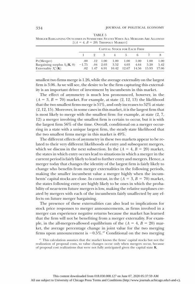
334 journal of political economy
All
smallest two firmsmerge is 1.26, while the average externality on the largestfirm is 3.06. As we will see, the desire to be the firm capturing this external-ity is an important driver of investment by incumbents in this market.The effect of asymmetry is much less pronounced, however, in the
(A 5 3, B 5 70) market. For example, at state (2, 12, 13) the likelihoodthat the two smallest firmsmerge is 51%, and only increases to 52%at state(2, 12, 15).Moreover, in some cases in thismarket, it is the largest firm thatis most likely to merge with the smallest firm: for example, at state (2, 7,12) a merger involving the smallest firm is certain to occur, but it is withthe largest firm 56% of the time. Overall, conditional on a merger occur-ring in a state with a unique largest firm, the steady state likelihood thatthe two smallest firms merge in this market is 49%.The different effects of asymmetry in these twomarkets appear to be re-
lated to their very different likelihoods of entry and subsequent mergers,which we discuss in the next subsection. In the (A 5 4, B 5 20) market,the states in which entry occurs lead to situations in which a merger in thecurrent period is fairly likely to lead to further entry andmergers.Hence, amerger today that changes the identity of the largest firm is fairly likely tochange who benefits from merger externalities in the following periods,making the smaller incumbent value a merger highly when the incum-bents’ capital stocks are close. In contrast, in the (A 5 3, B 5 70)market,the states following entry are highly likely to be ones in which the proba-bility of near-term future mergers is low, making the relative surpluses cre-ated by mergers with each of the incumbents fairly unaffected by any ef-fects on future merger bargaining.The presence of these externalities can also lead to implications for
stock price responses to merger announcements, as firms involved in amerger can experience negative returns because the market has learnedthat the firm will not be benefiting from a merger externality. For exam-ple, in the all-mergers-allowed equilibrium of the (A 5 4, B 5 20) mar-ket, the average percentage change in joint value for the two mergingfirms upon announcement is 20.5%.47 Conditional on the two merging
TABLE 5Merger Bargaining Outcomes in Symmetric States When AllMergers Are Allowed
[(A 5 4, B 5 20) Triopoly Market]
Capital Stock for Each Firm
1 2 3 4 5 6 7 8
Pr(Merger) .00 .12 1.00 1.00 1.00 1.00 1.00 1.00Bargaining surplus Sij(K, 0) 21.75 .04 2.03 3.52 4.03 4.64 5.20 5.42Externality X ij
k ðKÞ .02 1.47 6.91 10.42 12.67 14.56 15.93 17.06
47 This calculation assumesrealization of proposal costs,of proposal cost realizations t
This content downl use subject to University of Chic
that theso valuehat were
oaded froago Pres
markechangnot fu
m 018.s Terms
t knowes occully anti
030.008 and C
s the firr onlycipated
.127 on onditions
ms’ capwhen mgiven th
June 07, (http://w
ital stockergers oe capita
2020 05:ww.jour
s but nccur, bel state K
37:59 Anals.uch
ot thecause.
Micago.edu/t-and-c).

internal versus external growth 335
firms being unequal in size, the average percentage change in value forthe larger merging firm is20.6%, while it is 0.1% for the smaller mergingfirm.48 The small value change for the small firm occurs because in moststates in which mergers occur a merger is certain to occur and involvethe small firm. In such cases, the only surprise can involve which firm itmerges with, and often this is fully anticipated as well.
2. Effects of Fixed Merger Policies
Table 6 reports the outcomes in these twomarkets when all mergers are al-lowed. As in our previous two-firm analysis, in bothmarkets switching fromthe no-mergers-allowed policy to the all-mergers-allowed policy has a signif-icant negative impact on steady state consumer value, here due to the in-dustry spendingmuch less time in triopoly andmore time induopoly stateswhen allmergers are allowed.However, in other respects, when allmergersare allowed these two markets display some important differences fromeach other and from the outcomes we discussed in section III.In the (A 5 3, B 5 70) market, mergers almost never happen when all
mergers are allowed. The reason is that the industry settles into a roughlysymmetric duopoly in which each firm has roughly 12 units of capital, andin which entry is very unlikely.49 For entry to happen with positive proba-bility one or both incumbents need to experience a great deal of depreci-ation. For example, with symmetric incumbents entry only starts to have apositive probability once bothhave depreciated to 8 units of capital or less.As in section III, the prospect of entry for buyout incents entry (when nomergers are allowed entry would not happen unless both symmetric in-cumbents had less than 3 units of capital), but still not enough for entryto be more than a rare occurrence. Compared to the no-mergers-allowedsteady state, the shift from triopoly to duopoly states reduces investment,causing the level of capital and AV to fall, although in contrast to the du-opoly situation in section III producer value does increase.Allowing all mergers in the (A 5 4, B 5 20) market instead leads to a
27.5% likelihood of entry. This happens because the industry convergesto a duopoly outcome in which two active firms each have roughly 8 unitsof capital and in each period there is approximately a 25% chance of an
48 In such cases, the large firm has on average 6.96 units of capital, while the small firmhas 2.07 units of capital. Positive value changes occur for the large firm only 1.5% of thetime and only when the observed merger was the only merger with positive probabilitybut that probability was less than 1. Negative returns occur for the small firm only 2.4%of the time and only when there are positive probabilities of it merging with each of twodifferently sized larger firms.
49 For example, starting from a symmetric state in which three firms each have 5 units ofcapital, a merger is certain to happen; after that, the two remaining firms converge over anumber of periods to having roughly 12 units of capital each, until another entry eventoccurs.
This content downloaded from 018.030.008.127 on June 07, 2020 05:37:59 AMAll use subject to University of Chicago Press Terms and Conditions (http://www.journals.uchicago.edu/t-and-c).

336 journal of political economy
All
entrant building 1 unit of capital.50 When this happens, the entrant is ac-quired by one of the two incumbents, investments again lead to a situationin which the two firms each have roughly 8 units of capital, and the processrepeats itself. In contrast to what we have seen in the duopoly markets ofsection III and the (A 5 3, B 5 70) market, producer value increasesenough to make steady state AV almost identical to that when no mergersare allowed, and the average total capital level is higher (14.3 rather than14.0). The greatly improved relative AV performance of the all-mergers-allowed policy is largely driven by the incumbents’ investment responsesto the bargaining externality. When there are two incumbent firms withcapital levels that are not too far apart and an entrant with no capital, thisexternality incents each incumbent to investmore in an attempt tobecomethe largest firm in the industry, and then benefit from its rival acquiring theentrant. Moreover, this enhanced incumbent investment incentive alsocurbs the amount of entry-for-buyout behavior. For example, in state (0,
TABLE 6Performance Measures for the Triopoly Markets
Performance Measure
(A 5 3, B 5 70) (A 5 4, B 5 20)
NoMergers/MPP CV/Static CS
AllMergers/MPP AV
StaticAS
NoMergers/MPP CV/Static CS
AllMergers/MPP AV
StaticAS
Average consumer value 209.9 180.0 180.2 161.9 145.1 146.4Average incumbent value 199.3 221.7 221.7 126.7 143.0 142.2Average entrant value .0 .0 .0 .0 .5 .7Average blocking costAverage aggregate value 409.2 401.7 401.7 288.7 288.6 289.3Average price 1.91 1.99 1.99 2.20 2.30 2.29Average quantity 76.6 71.0 70.9 36.0 34.0 34.2Average total capital 26.1 23.2 23.2 14.0 14.3 14.6Merger frequency .4 .4 27.5 29.4Percentage in monopoly .0 .0 .0 .0 .0 .0Percentage in duopoly 24.5 99.6 99.6 .6 97.9 96.7Percentage with oneAV/AS-enhancing merger .0 .0 46.0 .0 5.8 1.0
Percentage with twoAV/AS-enhancing mergers .7 .4 .0 .0 23.8 31.7
Percentage with threeAV/AS-enhancing mergers 74.8 .0 .4 .0 .0 .3
State (0, 0, 0) CV 136.4 132.3 132.5 111.0 111.5 111.8State (0, 0, 0) AV 143.4 147.6 147.8 134.4 124.3 125.7
50 For example, starting fromcapital, a merger is certain tonumber of periods toward havoccurs.
This content downl use subject to University of Chic
a symmetric state in which thhappen; after that the two reming roughly 8 units of capital e
oaded from 018.030.008.127 on Jago Press Terms and Conditions
ree firms eaaining firmach, until an
une 07, 202(http://www
ch have 5 us convergeother entr
0 05:37:59 A.journals.uc
Note.—All values are ex ante (beginning of period) values, except the percentage inmonopoly, percentage in duopoly, and state (0, 0, 0) CV and AV, which are at the Cournotcompetition stage.
nits ofover ay event
Mhicago.edu/t-and-c).

internal versus external growth 337
7, 7), the vector of expected investments is (0.6, 1.2, 1.2) and (0.3, 1.7, 1.7)under the no-mergers and all-mergers-allowed policies, respectively.51
In bothmarkets a static aggregate-surplus-basedpolicy allowsmanymerg-ers. For example, in the (A 5 3, B 5 70) market, when a merger is pro-posed between symmetric firms the merger is always approved if the firmsare each smaller than the nonmerging rival, and is often approved even ifthey are larger than the rival. The static policy is not quite so lenient in the(A 5 4, B 5 20) market, but is still very permissive: for example, when amerger is proposed between symmetric firms facing a rival with 10 unitsof capital, themerger will be approved if and only if themerging firms eachhave nomore than 5 units of capital. As a result, the outcomes in thesemar-ketswhen the authority follows a static aggregate-surplus-basedpolicy is veryclose to that when all mergers are allowed. In contrast, a static consumer-surplus-based policy essentially allows no mergers in these markets.
3. Markov Perfect Merger Policy
Because entry against duopolists is very unlikely in the (A 5 3, B 5 70)market, with anAV criterion theMarkov perfect policy’s treatment of a pro-posedmerger of two of three active firms is largely unaffected by any entry-for-buyout concerns. Without such concerns, this Markov perfect policy isquite permissive.52 For example, like the static aggregate-surplus-based pol-icy it always allows two symmetric firms to merge when each is no largerthan their nonmerging rival, and often allows them to merge even whenthey are larger.Given this leniency, the steady stateoutcomeunder theMar-kov perfect policy with an AV criterion is essentially identical to that whenall mergers are allowed. As with allowing all mergers, the Markov perfectpolicy therefore lowers steady state AV compared to a policy of allowingno mergers.53
51 Still, much of the entrant’s investment incentive comes from the prospect of beingacquired; e.g., in state (0, 7, 7) it would not invest at all if the incumbents were followingtheir all-mergers-allowed investment policies but no mergers were allowed.
52 The remaining factors tend to favor a permissive policy here: First, combining twofirms’ capital stocks increases aggregate surplus in many states. Second, the combinationreduces investment costs since investment costs are decreasing in firm size. Third, sinceinvestment by small firms in triopoly is often socially excessive (much as in duopoly), merg-ers of small firms that reduce their investments can be beneficial for aggregate value. TheMarkov perfect policy is, however, somewhat more stringent than the static policy whenthe nonmerging firm is not large; e.g., when the nonmerging rival has 4 units of capital,the Markov perfect policy allows a merger of symmetric firms as long as they have no morethan 6 units of capital, while the static policy would allow the merger even if they each have10 units of capital. The two policies become quite similar when the nonmerging firm hasmore than 8 units of capital.
53 Observe in table 6, however, that starting at state (0, 0, 0) the Markov perfect policyyields a higher AV than allowing no mergers. The Markov perfect policy outcome has allthree firms’ capital quickly reach a point at which a merger does not result in entry; thena merger occurs, followed by a future with a very low likelihood of entry. Note that the
This content downloaded from 018.030.008.127 on June 07, 2020 05:37:59 AMAll use subject to University of Chicago Press Terms and Conditions (http://www.journals.uchicago.edu/t-and-c).

338 journal of political economy
All
In the (A 5 4,B 5 20)market, entry happens but the investment incen-tives noted above curtail the extent of the investment inefficiency followinga merger. Overall, the Markov perfect policy with an AV criterion is againfairly lenient and allows two symmetric firms to merge whenever they areeach smaller than their nonmerging rival. Indeed, in thismarket it ismuchmore lenient than the static aggregate-surplus-based policy. As a result, thesteady state outcomeunder theMarkov perfect policy with the AV criterionis again very similar to that under the all-mergers-allowed policy.54
In summary, firms respond very differently in these two triopoly marketsto policies allowing mergers, driven by the differing likelihoods of entry inthese markets. In both markets, however, the negative effects of entry forbuyout are either not present or limited, resulting in an AV-based Markovperfect policy that is fairly lenient, a contrast to our finding for duopoly insection III. Like the duopoly case, the resulting steady state outcome is notonly bad for consumers but fails to raise AVrelative to allowing nomergers,although the difference is minimal in the (A 5 4, B 5 20) market.
V. Conclusion
We have studied optimal merger policy in a dynamic industry model inwhich scale economies can be achieved through either investment (“inter-nal growth”) or merger (“external growth” ). In such a setting, an antitrustauthority’s merger approval decisions must weigh any increases in marketpower against the changes in productive efficiency caused by a merger,which are affected not only by the immediate cost reductions of the merg-ing parties due to their increased scale, but also by the investments of boththe merging parties and rivals following the merger.To shed light on this complicated problem we have developed and com-
putationally solved a dynamic model in which forward-looking Cournotfirms invest in capital to produce a homogeneous product. Our modelhas three significant innovations relative to previous computational dy-namic industry models. First each firm in each period can flexibly decidehowmany additional units of capital it wishes to purchase. Second, this in-vestment technology is (approximately) merger neutral in the sense thatthe investment opportunities available in the market are unchanged fol-lowing amerger, offering amuchmore attractive setting for studyingmerger
antitrust authority’s lack of commitment in this market is not very important because oncethe first merger occurs, future mergers are rare. Also, as in the (A 5 3, B 5 26) duopolymarket, in both of these triopoly markets the Markov perfect policy with a CV criterionyields a steady state equilibrium equivalent to the no-mergers-allowed policy.
54 In contrast to the results for the (A 5 3, B 5 70) market and the (A 5 3, B 5 26) du-opoly market of sec. III, here a commitment to the static aggregate-surplus-based policyinduces a slightly higher steady state aggregate value than the no-mergers-allowed policy,the all-mergers-allowed policy, and the Markov perfect policy.
This content downloaded from 018.030.008.127 on June 07, 2020 05:37:59 AM use subject to University of Chicago Press Terms and Conditions (http://www.journals.uchicago.edu/t-and-c).
internal versus external growth 339
policy than the original Pakes and McGuire (1994)/Ericson and Pakes(1995)model. Third, we introduce an antitrust authority as an active, max-imizing player that cannot commit to its future merger approval policy. Be-cause of the time inconsistency difficulties that arise in dynamic games theauthority is unable to achieve as high a level of welfare as an authority thatcan commit would be able to achieve.55
Inmuch of ourmain analysis, we have focused onmarkets with two firmsso as to be able to use the familiar and well-accepted Nash bargaining solu-tion. In addition, we have studied markets with three firms, using one par-ticular model of multifirm bargaining with externalities. Our analysis ofthese markets provides insights into the factors affecting optimal mergerpolicy when investment behavior and firm scale are critical determinantsof welfare, and shows how optimal policy in dynamic settings with invest-ment can differ in significant ways from what would be statically optimal.Specifically, we make five key observations.First, the desirability of approving a merger can depend importantly on
the investment behavior that will follow if it is or is not approved. However,this involvesmore than just the behavior of themerging firms, as the invest-ment behavior of outsiders to themerger (here, new entrants) can have sig-nificant welfare effects. In particular, when entrants (or, more generally,small firms) have higher investment costs than large established incum-bents, entry-for-buyout behavior can impose significant welfare losses andmake merger approvals much less attractive for an antitrust authority.Second, in theother direction, investment behaviors canbe greatly influ-
enced by firms’ beliefs about future merger policy. Importantly, when theantitrust authority adopts a less restrictive policy, this may spur entry-for-buyout behavior by firms seeking to be acquired.Third, the inability to commit may be costly for an antitrust authority. In
fact, in cases in which aggregate value is the true social objective, it can of-ten be better to endow the antitrust authority with a consumer value objec-tive (which roughly corresponds to the objective of most antitrust author-ities, including those in the United States and European Union).Fourth, the optimal antitrust policy formaximizing aggregate value in our
model can differ significantly from the optimal static policy that considers amerger’s effects only at the time it would be approved, although it may beeither more or less permissive than the static policy.Finally, externalities on rivals arising frommergers inmarkets withmore
than two firms can have significant effects on firms’ investment incentivesand thereby shape the antitrust authority’s optimal policy.At a more general level, the existing literature modeling merger policy
has largely neglected dynamic concerns. In a world in which the antitrust
55 In the appendix, we have also analyzed the case of an antitrust authority that can com-mit to its future merger approval rule.
This content downloaded from 018.030.008.127 on June 07, 2020 05:37:59 AMAll use subject to University of Chicago Press Terms and Conditions (http://www.journals.uchicago.edu/t-and-c).
340 journal of political economy
All
authority cannot commit fully to its future actions, analyzing such issues re-quiresmodeling the authority as a player who acts dynamically. The presentpaper is a first step in doing so in a truly dynamic setting. By proposing amerger-neutral investment technology that allows for complexmultiunit in-vestment choices and yet is tractable, it also contributes to the computa-tional industrial organization literature more generally.
References
Abel, A. 1979. Investment and the Value of Capital. New York: Garland.Benkard, C. L., A. Bodoh-Creed, and J. Lazarev. 2010. “Simulating the Dynamic Ef-
fects of Horizontal Mergers: U.S. Airlines.”Working paper, Dept. Econ., StanfordUniv.
Bernard, A., J. Eaton, J. B. Jensen, and S. Kortum. 2003. “Plants and Productivity inInternational Trade.” A.E.R. 93:1268–90.
Berry, S., and A. Pakes. 1993. “Applications and Limitations of Recent Advances inEmpirical Industrial Organization: Merger Analysis.” A.E.R. 83:247–52.
Bond, S., and J. van Reenen. 2007. “Microeconometric Models of Investment andEmployment.” In Handbook of Econometrics, vol. 6A, edited by J. J. Heckman andE. E. Leamer. Amsterdam: North Holland.
Bourreau, M., B. Jullien, and Y. Lefouilli. 2018. “Mergers and Demand-EnhancingInnovation.” TSE Working Paper no. 18-907, Toulouse School Econ.
Burguet, R., andR.Caminal. 2015. “BargainingFailures andMerger Policy.” Internat.Econ. Rev. 56:1019–41.
Cheong, K.-S., andK. L. Judd. 2000. “Mergers andDynamicOligopoly.”Working pa-per, Hoover Inst., Stanford Univ.
Cooper, R. W., and J. C. Haltiwanger. 2006. “On the Nature of Capital AdjustmentCosts.” Rev. Econ. Studies 73:611–33.
DeGraba, P., and G. L. Rosston. 2014. “The Proposed Merger of AT&T and T-Mobile: Rethinking Possible.” In The Antitrust Revolution: Economics, Competition,and Policy, 6th ed., edited by J. Kwoka. New York: Oxford Univ. Press.
Doraszelski, U., and M. Satterthwaite. 2010. “Computable Markov-Perfect IndustryDynamics.” RAND J. Econ. 41:215–43.
Ericson, R., and A. Pakes. 1995. “Markov-Perfect Industry Dynamics: A Frameworkfor Empirical Work.” Rev. Econ. Studies 62:53–82.
Farrell, J., and C. Shapiro. 1990. “Horizontal Mergers: An Equilibrium Analysis.”A.E.R. 80:107–26.
Fazzari, S. M., R. G. Hubbard, and B. C. Petersen. 1988. “Financing Constraints andCorporate Investment.” Brookings Papers Econ. Activity (1): 141–206.
Federico, G., G. Langus, and T. Valletti. 2018. “Horizontal Mergers and Product In-novation.” Internat. J. Indus. Org. 59:1–23.
Gans, J., and S. Stern. 2003. “The Product Market and the Market for ‘Ideas’: Com-mercialization Strategies for Technology Entrepreneurs.” Res. Policy 32:333–50.
Gowrisankaran,G. 1997. “Antitrust Policy Implications of aDynamicMergerModel.”Working paper, Dept. Econ., Univ. Minnesota.
———. 1999. “A Dynamic Model of Endogenous Horizontal Mergers.” RAND J.Econ. 30:56–83.
Hayashi, F. 1982. “Tobin’s Marginal q and Average q: A Neoclassical Interpretation.”Econometrica 50:213–24.
Hollenbeck, B. 2017. “Horizontal Mergers and Innovation in Concentrated Indus-tries.”Workingpaper,AndersonSchoolManagement,Univ.California,LosAngeles.
This content downloaded from 018.030.008.127 on June 07, 2020 05:37:59 AM use subject to University of Chicago Press Terms and Conditions (http://www.journals.uchicago.edu/t-and-c).

internal versus external growth 341
Jeziorski, P. 2015. “Empirical Model of Dynamic Merger Enforcement: ChoosingOwnership Caps in U.S. Radio.”Working paper, Haas School Bus., Univ. Califor-nia, Berkeley.
Jones, C. I. 2005. “The Shape of Production Functions and the Direction of Techni-cal Change.” Q.J.E. 120:517–49.
Lyons, B. 2002. “Could Politicians Be More Right than Economists? A Theory ofMerger Standards.” CCP Working Paper no. 02-01, Univ. East Anglia.
Matsushima,N. 2001. “HorizontalMergers andMergerWaves in a LocationModel.”Australian Econ. Papers 40:263–86.
Motta, M., and E. Tarantino. 2018. “The Effect of Horizontal Mergers, When FirmsCompete in Prices and Investments.”Working paper, Dept. Econ. and Bus., Univ.Pompeu Fabra.
Motta,M., andH.Vasconcelos. 2005. “EfficiencyGains andMyopicAntitrustAuthor-ity in a Dynamic Merger Game.” Internat. J. Indus. Org. 23:777–801.
Nilssen, T., and L. Sorgard. 1998. “Sequential Horizontal Mergers.” European Econ.Rev. 42:1683–1702.
Nocke, V., andM.D.Whinston. 2010. “DynamicMerger Review.” J.P.E. 118:1200–51.Pakes, A., andP.McGuire. 1994. “ComputingMarkov PerfectNashEquilibrium:Nu-
merical Implications of a Dynamic Differentiated Product Model.” RAND J. Econ.25:555–89.
Pittman, R., and Y. Li. 2013. “AT&T and T-Mobile: Economies as an Antitrust De-fense Applied.” J. Competition Law and Econ. 9:49–63.
Rasmusen, E. 1988. “Entry for Buyout.” J. Indus. Econ. 36:281–300.Syverson, C. 2004. “Market Structure and Productivity: A Concrete Example.” J.P.E.
112:1181–1222.Williamson, O. E. 1968. “Economies as an Antitrust Defense: The Welfare Trade-
offs.” A.E.R. 58:18–36.
This content downloaded from 018.030.008.127 on June 07, 2020 05:37:59 AMAll use subject to University of Chicago Press Terms and Conditions (http://www.journals.uchicago.edu/t-and-c).