Market Optimism and Merger Waves

Klaus Guglera

Dennis C. Muellerb

Michael Weichselbaumerc

B. Burcin Yurtoglud

Abstract

One of the most conspicuous features of mergers is that they come in waves, and that these

waves are correlated with increases in share prices and price/earnings ratios. We argue that

stock market booms and merger waves are both driven by increases in optimism in financial

markets, and discuss two behavioral hypotheses about mergers – the managerial discretion

and overvaluation hypotheses – that claim that merger waves are driven by market optimism.

We also develop the hypothesis and present evidence that optimism in bond markets can

cause mergers. We also briefly consider and reject two neoclassical hypotheses that claim to

account for mergers waves. Empirical support for the managerial theory is provided by

evidence that the amounts of assets acquired by companies increase as optimism in financial

markets increases, and that the returns to acquiring companies’ shareholders are inversely

related to market optimism at the time of mergers. Our measures of market optimism are

also shown to explain managerial choices of finance for mergers. Thus, we find that

optimism in financial markets explains the amount of assets acquired through mergers at a

point in time, the choice of means for financing the mergers, and the returns to the acquirers’

shareholders following the mergers.

a

WU Vienna University of Economics and Business, Department of Economics, Augasse 2-

6, 1090 Vienna, Austria; E-Mail: klaus.gugler@wu.ac.at. b

University of Vienna, Department of Economics, BWZ, Bruennerstrasse 72, 1210, Vienna,

Austria, E-Mail: dennis.mueller@univie.ac.at. c

Vienna University of Technology, Institute of Management Science, Theresianumgasse 27,

1040 Vienna, Austria, E-Mail: michael.weichselbaumer@tuwien.ac.at. d

WHU – Otto Beisheim School of Management, Burgplatz 2, 56179 Vallendar, Germany, E-

Mail: burcin.yurtoglu@whu.edu.

The research in this article was supported in part by the Austrian National Bank’s Jubiläumsfond, Project

8861.

1

Two well-established stylized facts about mergers in the United States are that they

come in waves, and that these waves occur during major advances in share prices.1 The first

major wave occurred at the end of the 19th

century. Subsequent waves occurred at the ends

of the 1920s and 1960s. Each of these waves was accompanied by dramatic surges in stock

prices. Each wave came to a close when stock prices plummeted. This pattern has been

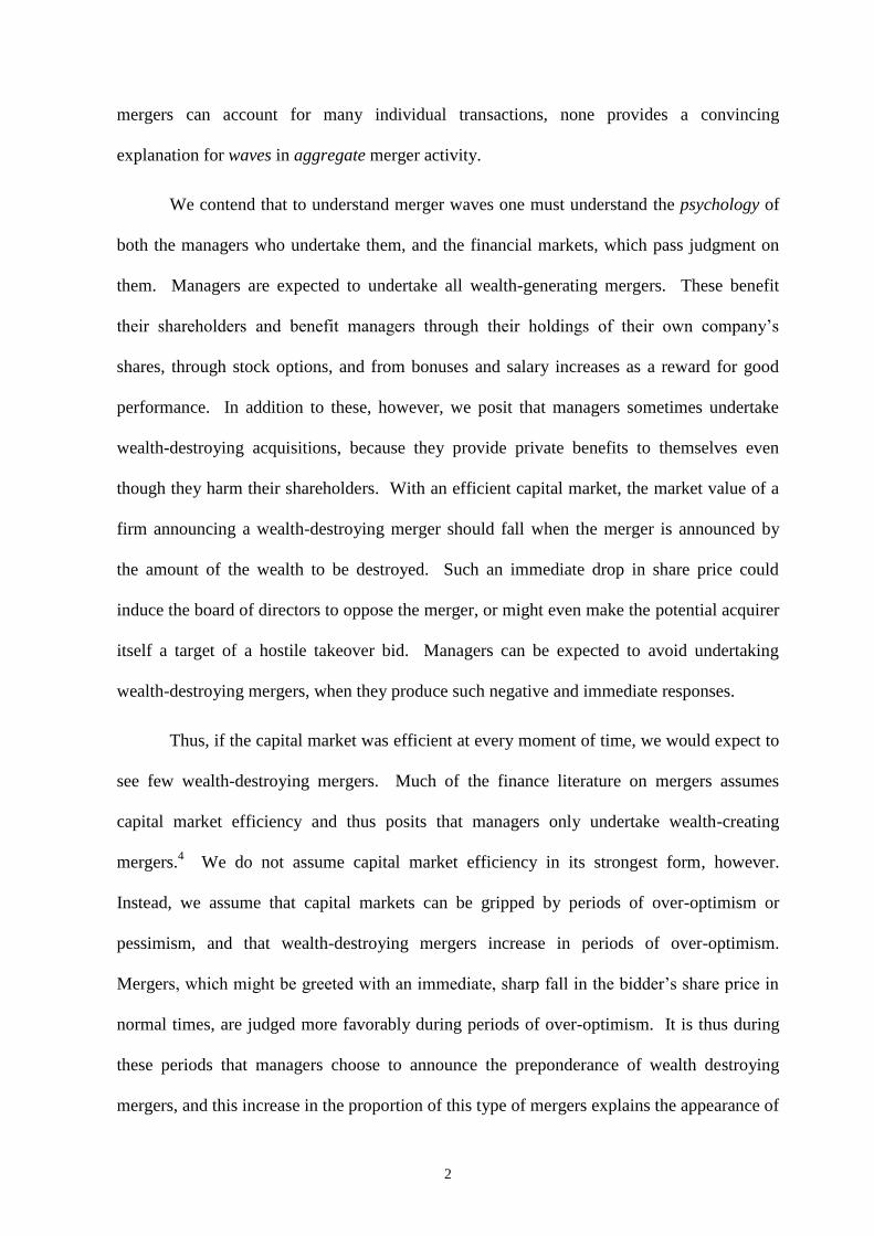
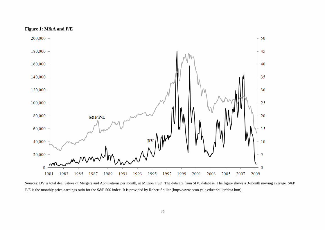
repeated in the two most recent waves. Figure 1 presents a three-month moving average of

the amounts of assets acquired since the beginning of the 1980s and Shiller’s aggregate price-

earnings ratio (P/E).2 A steady rise in the aggregate P/E is apparent until its peak in 2000.

This rise is matched by the rise in merger activity. Some students of mergers interpret the

blips in mergers during the 1980s as a wave, but it seems obvious to us that the rise in

mergers during the 1980s was part of the long wave that culminated at the end of the century,

and not a separate wave. The 21st century begins with a sharp fall in both share prices and

merger activity, but starting around 2003 both indexes begin to rise reaching new peaks in

2007. As the financial crisis takes hold, both share prices and mergers decline precipitously.

Any general theory of mergers must account for both their wave pattern and the association

of the peaks in merger activity with peaks in share prices and price-earnings ratios. We offer

such an account.

An enormous number of hypotheses have been advanced to explain mergers. They

typically do not purport to explain merger waves, however, but rather specific sorts of

mergers – horizontal mergers to achieve economies of scale or market power, vertical

mergers to reduce transaction costs or raise entry barriers, and so on.3 Why should the

acquisition of market power become particularly attractive when share prices rise, and lose its

attraction when they fall? Why is the pursuit of efficiency through cost-reducing mergers not

more attractive during recessions, when competitive pressures are intense, than in times of

economic prosperity when share prices are high? Although traditional explanations for

2

mergers can account for many individual transactions, none provides a convincing

explanation for waves in aggregate merger activity.

We contend that to understand merger waves one must understand the psychology of

both the managers who undertake them, and the financial markets, which pass judgment on

them. Managers are expected to undertake all wealth-generating mergers. These benefit

their shareholders and benefit managers through their holdings of their own company’s

shares, through stock options, and from bonuses and salary increases as a reward for good

performance. In addition to these, however, we posit that managers sometimes undertake

wealth-destroying acquisitions, because they provide private benefits to themselves even

though they harm their shareholders. With an efficient capital market, the market value of a

firm announcing a wealth-destroying merger should fall when the merger is announced by

the amount of the wealth to be destroyed. Such an immediate drop in share price could

induce the board of directors to oppose the merger, or might even make the potential acquirer

itself a target of a hostile takeover bid. Managers can be expected to avoid undertaking

wealth-destroying mergers, when they produce such negative and immediate responses.

Thus, if the capital market was efficient at every moment of time, we would expect to

see few wealth-destroying mergers. Much of the finance literature on mergers assumes

capital market efficiency and thus posits that managers only undertake wealth-creating

mergers.4 We do not assume capital market efficiency in its strongest form, however.

Instead, we assume that capital markets can be gripped by periods of over-optimism or

pessimism, and that wealth-destroying mergers increase in periods of over-optimism.

Mergers, which might be greeted with an immediate, sharp fall in the bidder’s share price in

normal times, are judged more favorably during periods of over-optimism. It is thus during

these periods that managers choose to announce the preponderance of wealth destroying

mergers, and this increase in the proportion of this type of mergers explains the appearance of

3

merger waves. We present evidence linking merger activity to measures of optimism in both

equity and bond markets.

The importance of the psychology of managers and financial markets in our theory

places it among the behavioral theories of economics and finance.5 Shleifer and Vishny

(2003) (hereafter S&V) have offered an alternative behavioral theory of mergers, which

makes some of the same predictions as ours does. Although some of the evidence we present

is consistent with the S&V theory, some is not. We discuss their theory below along with the

tests to discriminate between them.

Our behavioral theory and that of S&V can be contrasted with the neoclassical

theories of merger waves of Jovanovic and Rousseau (2002, J&R) and Harford (2005). J&R

extend the q-theory of investment to mergers. Mergers occur during stock market booms,

because average qs are higher then. Harford posits that industry shocks cluster at certain

times producing merger waves. Being neoclassical, both theories assume that managers

maximize their shareholders’ wealth, and thus implicitly that they increase this wealth. This

prediction is at odds with much of the literature on the effects of mergers on acquirers’

shareholders, and with the results of the effects of mergers presented in this article. We do

not, therefore, explicitly test these neoclassical theories, but only comment upon them from

time to time where our evidence pertains to them.

We proceed as follows. Because of the important role it plays in our theory, we begin

with a review of the literature on the psychology of financial markets. In Section II, we

present the logic underlying the managerial theory of mergers. S&V’s overvaluation

hypothesis is discussed in Section III. Section IV develops the main hypotheses to be tested.

The data and methodologies employed are discussed in Section V. Section VI presents the

results for the tests of the theory. Conclusions are drawn in the final section.

4

I. The Psychology of Financial Markets

A. Stock Markets

If it is firm i’s profits in period t, ki its cost of capital, and i’s managers either pay out

its profits as dividends and interest or reinvest them at returns equal to ki, then the value of

the firm at time zero is given by

0

0 (1 )

iti t

t i

Vk

(1)

Thus, today’s share price should have a definite relationship to a firm’s future earnings and

dividends. In a pioneering study, Robert Shiller (1981) showed that swings in stock prices in

the United States over the 20th

century were far greater than could be accounted for by

subsequent movements in earnings and dividends.6 During the late 1920s shareholders were

far more optimistic about future earnings and dividends than was warranted by both the

actual dividends and earnings that were to come, and those that one might have expected

based on past dividends and earnings experience. During the 1930s shareholders became far

more pessimistic than would prove to be warranted.

The extent to which this over-optimism and pessimism can go is dramatically

revealed by the data from the late 1990s. Assuming an average rate of growth of gi from now

to infinity, (1) becomes

0

0

(1 )

(1 )

t

io i ioi t

t i i i

gV

k k g (2)

if ki > gi. This implies a price/earnings ratio for firm i equal to 1/(ki - gi). As can be seen

from Figure 1, at the peak of the 1990s stock market boom, the aggregate P/E topped 40. If

we assume a ki of 0.12, roughly the average return on stocks over the period 1928-2004,7 then

a P/E of 40 implies an expected, perpetual growth rate of 0.095 – more than four times the

5

average growth rate over the same period. At the 1990s stock market peak, shareholders

appeared to believe that the average firm’s profits would grow indefinitely at a rate far above

any that had ever been seen before.

This extreme optimism typifies stock market booms. Galbraith (1961, p. 8) observed

that an “indispensable element of fact” during stock market bubbles is that individuals “build

a world of speculative make-believe. This is a world inhabited not by people who have to be

persuaded to believe but by people who want an excuse to believe.” These excuses to believe

take the form of “theories” as to why share prices should rise to unprecedented levels, why

the economy has entered a “new era” (Shiller, 2000, Ch. 5). Prominent among these are

“theories” about wealth increases from mergers. Shiller gives an example from the stock

market boom and merger wave at the beginning of the 20th

century. “The most prominent

business news in the papers in recent years had been about the formation of numerous

combinations, trusts, and mergers in a wide variety of businesses, stories such as the

formation of U.S. Steel out of a number of smaller steel companies. Many stock market

forecasters in 1901 saw these developments as momentous, and the term community of

interest was commonly used to describe the new economy dominated by them” (Shiller,

2000, p. 101, italics in original). Shiller quotes a New York Times’ editorial from April 1901,

which prophesizes that the U.S. Steel merger will avoid “much economic waste” and effect

“various economies coincident to consolidation.” It predicts similar benefits from mergers in

railroads. Such optimism explains why U.S. Steel’s share price soon soared to $55 from the

$38 it was floated at in 1901. By 1903 it had plunged to $9 (Economist, 1991, p. 11).

Similar over-optimism appears to have been a major cause of the first great merger wave.

The literature provides convincing evidence that the abnormally large volume of

mergers formed in 1897-1900 stemmed from a wave of frenzied speculation in asset

values. Several students of the early merger movement agree that the excessive demand

for securities was an impelling force in the mass promotion of mergers after 1896

(Markham, 1955, p. 162).

6

A second example of the over-optimism that can feed merger waves comes from the

1960s. During this wave, the so-called conglomerates undertook a series of diversification

mergers. Each new merger announcement was greeted by an increase in the conglomerate’s

share price. One explanation for this given in both the popular and academic literatures was

that the conglomerates were engaging in “P/E magic.”8 Because of the market’s optimism,

conglomerates traded at P/Es as high as 30. A conglomerate would announce that it was

acquiring, say a steel company, with a P/E of 10. The steel company’s low P/E obviously

suggests that the market anticipated slower future earnings growth than for the conglomerate.

Upon the merger announcement, however, the market would reevaluate the earnings of the

steel company using the conglomerate’s P/E. Thus, if the steel company had earnings of $10

million and a market value of $100 million, these earnings would create $300 million in

value for the conglomerate, easily allowing it to buy the steel company at a hansom premium

and still have a positive gain from the transaction. The obvious question to be asked is

whether the conglomerates would be able to generate growth in the steel firm’s earnings to

justify a P/E of 30. The conglomerates’ performance once the stock market bubble burst

indicates that they were not able to generate this growth.9 The conglomerates’ P/E magic of

the sixties resembles the kind of Ponzi scheme that Shiller (2000, pp.64-66) claims

characterizes all stock market bubbles.

The over-optimism of stock market booms figures prominently, but in somewhat

different ways in the two behavioral theories of mergers discussed later.

B. Bond Markets

Bonds carry commitments for fixed payments to bondholders, and they must receive

their interest payments before funds are distributed to shareholders. Bonds thus entail less

risk than stocks. Periods of optimism or pessimism can also affect bond markets, however.

Optimistic bond holders will perceive less risk in corporate securities, and be willing to

7

accept less of a premium over the Federal Funds Rate to hold a particular bond. Thus, the

Spread between the Federal Funds Rate and the Commercial & Industrial Loan Rate (the

interest rate blue chip companies pay to borrow funds, hereafter C&ILR) can be regarded as a

measure of the degree of optimism, or the degree of perceived risk in the bond market.

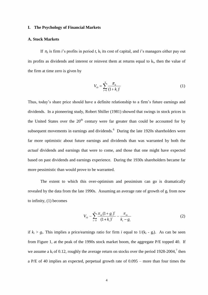
Figure 2 plots merger activity, the real, i.e. CPI adjusted, C&ILR and the Spread

since 1980. Although it exhibits a secular downward trend, the C&ILR rises during both

merger waves. Thus, these waves cannot be explained by a fall in borrowing costs. In

contrast, the Spread rises during the first wave, but then falls and remains relatively constant

during the second indicating continuing optimism in the bond market toward the end of the

decade. This optimism in the bond market, we believe, reinforced the optimism apparent in

the equity market and helps explain the second merger wave. It also explains the greater use

of debt to finance mergers in the second wave, which we document below. Consistent with

our interpretation of the Spread as a measure of optimism, it climbs steeply once the financial

crisis hits in 2008, while the Federal Funds Rate (not shown) falls just as precipitously.10

That the two variables appear to measure different phenomena is also evidenced by the

correlation coefficient between them of -0.71, significant at the 1% level.

Companies must pay the C&ILR to borrow funds or something higher, if they are

perceived to have higher risk. By this measure financing costs actually rose during both of

the recent waves as can be seen in Figure 2. Harford (2005) argues that merger waves occur

when many industries experience simultaneous shocks, and borrowing costs fall. However,

Harford did not use the C&ILR or some similar measure of interest rates to measure

borrowing costs, but rather the Spread with the Federal Funds Rate – our measure of

optimism in the bond market. Thus his tests of the neoclassical industry shocks hypothesis

actually incorporate some of the behavioral elements included in our theory.

8

II. The Managerial Theory of Mergers

Robin Marris (1964, 1998) was the first to posit growth as an objective for managers,

and presented considerable evidence that managers’ pecuniary and “psychic” incomes were

both linked to the growth of their firm. Recent evidence has confirmed the link between

managerial compensation and growth specifically with respect to growth through mergers.11

One study of bank mergers found that managerial incomes increased following mergers even

when their share prices fell (Bliss and Rosen, 2001).

The constraint on managers’ pursuit of growth is the threat of takeover, which can be

assumed to be inversely related to Tobin’s q. Thus, managers’ utility can be expressed as a

function of the growth of their firms, g, and q, ,U U g q , where 0U g ,

22 0U g , 0U q , and 22 0U q .

12 Defining M as the assets acquired through

mergers, setting g = g(M), and maximizing ,U g q with respect to M yields the following

first order condition:

( / )( / ) ( / )( / )U g g M U q q M (3)

Since 0U g , / 0g M , and 0U q , (3) cannot be satisfied if 0q M . For

any merger that increases q no tradeoff between growth and security from takeovers exists.

Growth-maximizing managers undertake all mergers that increase q. Their behavior differs

from managers who maximize shareholder wealth only with respect to mergers that decrease

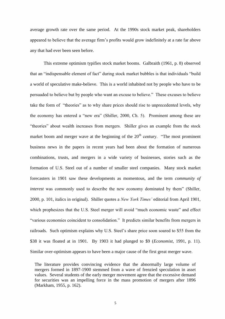
q. Figure 3 (left panel) depicts the relationship in eq. 3 for mergers that lower q. When no

mergers of this type are undertaken, q is at its maximum and the risk of takeover is

minimized. When - 0N

U q q M , managers undertake MN of value destroying

mergers.

9

During a stock market boom investors are more willing to accept new news as good

news. Merger announcements, that would under normal conditions result in large declines in

acquirers’ share prices, produce only modest declines during a stock market boom, or even

share price increases. Thus, the relationship between q and M shifts from its normal level,

say line N in Figure 3 (right panel), to something like B in a boom. This shifts

U q q M to the right, as in Figure 3. The firm acquires more assets through

mergers, MB, since q does not drop by as much or perhaps even rises when a wealth-

destroying merger is announced.

III. The Overvalued Shares Hypothesis (OVH)

Our main focus is on the managerial theory of mergers. Because both it and the

overvaluation theory of S&V (2003) relax the assumptions that mergers create wealth and

capital markets are efficient, however, we briefly describe their theory here so that later we

can point out where the predictions of the two differ.

Some firms’ share prices are assumed to be overvalued in stock market booms. Their

managers know their shares are overvalued, and wish to protect their shareholders from the

wealth loss that will come when the market lowers its estimates to their warranted levels.

They accomplish this by exchanging their overvalued shares for the real assets of another

company. Targets’ managers are assumed to have short time horizons, so they too gain by

“cashing in” their stakes in their firms at favorable terms. Under the S&V theory, mergers do

not destroy wealth they merely transfer it from the unlucky shareholders who wind up

holding the acquirers’ overvalued shares, when the market corrects its mistake, to the

acquirers’ shareholders.

The same is true of the explanation for merger waves put forward by Rhodes-Kropf

and Viswanathan (2004, hereafter RKV). While S&V emphasize the motivation of the

10

managers of the acquiring companies, RKV focus on the shareholders of the targets. They

are willing to accept the overvalued shares of bidders during a wave, according to RKV,

because during a stock market boom targets’ shareholders have difficulty distinguishing

whether a bidder’s shares have a high price because they are overvalued or because of

possible synergies from the merger. RKV devote little space to the motivations of the

bidders’ managers claiming only that they expect synergies form the mergers, but “make

mistakes” (RKV, 2004, p. 2709). Given all of the evidence that mergers on average destroy

wealth, it is difficult to believe that bidders’ managers are unaware of the risks they are

taking on behalf of their shareholders when they offer high premiums to acquire companies

during a merger wave.

IV. Testing the Managerial Theory of Mergers

A. The Causes of Mergers

The managerial theory assumes that managers can always obtain private benefits from

increasing their firm’s size of through mergers. In times of normal optimism, when financial

markets come close to exhibiting rational expectations, announcements of wealth destroying

acquisitions are greeted with sharp declines in share price and are either not attempted or

cancelled soon after the announcements. When optimism in financial markets is high,

wealth-destroying mergers increase in frequency, because they do not elicit such negative

responses from the market.

Optimism in financial markets can be thought of as taking two forms – firm-specific

optimism about the prospects of particular firms, and general optimism that prevails across

the entire market. Thus, in normal times, a given firm may be overvalued because of great

optimism about its prospects or management, and the announcement of a wealth-destroying

merger is greeted favorably. Alternatively, a company may not be overvalued, but great

optimism in the market exists, and the announcement of a wealth-destroying merger is again

11

greeted favorably. During stock market booms many individual firms are overvalued and

general optimism prevails across the equity market. During such times wealth-destroying

mergers appear in great numbers.

We employ two measures of general optimism in financial markets, the aggregate P/E

and the Spread between the Federal Funds Rate and the C&ILR. At any point in time, there

will be a level of the S&P 500 that is warranted by the future growth in profits and dividends.

Values of the S&P 500 above this level represent general over optimism, values below

pessimism (negative optimism). As discussed above, the Spread captures attitudes toward

risk in bond markets and thus measures optimism in bond markets.

When constructing a measure of a firm’s overvaluation, we encounter a

methodological difficulty. If we can identify overvalued firms, so too presumably can the

capital market and the firms cease to be overvalued. This conundrum notwithstanding,

several studies have constructed measures of overvaluation (Verter, 2002; Ang and Cheng,

2003; Dong, Hirshleifer, Richardson and Teoh, 2005; and Rhodes-Kropf, M., David. T.

Robinson, and S. Viswanathan, 2005, hereafter RKRV). These measures typically involve

ratios of market to book value of equity or their reciprocal. We assume that all firms in an

industry13

have the same costs of capital and expected growth rates, and use equation 2 to

estimate 1/( ki - gi) for a typical firm by regressing the market values of all firms in the

industry on their profits for a period of time when, based on the aggregate S&P P/E ratio,

shares in aggregate do not appear to be overpriced. Call this estimate of 1/( ki - gi), . Using

this we predict firm i’s market value in year t as

it itV (4)

We then create a measure of a firm’s overvaluation in any year, Oit , as

it it itO V V (5)

12

We use this measure of overvaluation to test the overvaluation theory of mergers.

In addition to Oit , the P/E, and the Spread (S), several control variables are included

in our model of acquisitions. The dependent variable is defined as the amount of assets

acquired in period t by firm i, Mit , measured as the amount paid for the target. Holding Mit

constant, the larger the size of a potential acquirer, the less impact the acquisition has on its

market value. Thus, the curve relating q to M in Figure 3 should be flatter, the larger the size

of the acquiring firm (TA) relative to the target, M. We measure the size of the acquirer as

the natural log of the lagged value of its total assets, ln(TAit-1). A second justification for

including size in the equation is that the costs of taking over a firm and replacing its

managers should grow with the size of the company. Managers of large companies have

more discretion, therefore, to make bad acquisitions. For these reasons, we expect assets

acquired through mergers to vary positively with firm size.

For a firm that over invests, the marginal return on investment is below its

neoclassical cost of capital. Raising funds externally, therefore, will seem more expensive

than using internal cash flows. Cash flow has, therefore, been a key variable in tests of

managerial theories of the determinants of corporate investment and R&D.14

Lagged cash

flow, CFit-1, is thus included as an additional explanatory variable.

Cash flow is unlikely to be large enough to finance large acquisitions, and thus these

companies must resort to equity and bond markets. A company is likely to have more

difficulty floating bonds to finance a merger, the larger its leverage is. We thus include

lagged leverage, Lit-1, in the model.

J&R’s q-theory of mergers assumes that the market correctly evaluates a firm’s

market value based on its expected future profits, that Tobin’s q proxies for managerial

talent, and thus companies with high qs undertake more mergers. Alternatively, if the market

13

may overvalue a company’s shares, q might serve as an alternative measure of overvaluation

to the one we construct. As we shall see below, Tobin’s q and our measure of overvaluation

are highly correlated. When both are included in the determinants equation, our measure is

significant and with the correct sign, q is insignificant. Thus, we did not include q in the

model.

We thus come up with the following model to explain the amount of asserts acquired

through mergers.

Mit = a + bOit + cP/Et + dSt + e ln(TAit-1) + fCFit-1 + gLit-1 + μit (6)

with predictions, b > 0, c > 0, d < 0, e > 0, f > 0, and g < 0.

Because the Spread is part of the borrowing costs of firms, a negative coefficient on

this variable might simply be interpreted as evidence that firms invest less in mergers, when

borrowing costs are high. To test whether the Spread in (6) really is capturing something

other than borrowing costs, we estimate it adding the Federal Funds Rate in t, FFt.

Mit = a + bOit + cP/Et + dSt + e ln(TAit-1) + fCFit-1 + gLit-1 + hFFt + μit (7)

If the Spread is merely measuring a firm’s cost of capital, then St and FFt should have the

same coefficients, d = h, since both are parts of a firm’s borrowing costs and sum to C&ILR.

A firm should be indifferent between a one percentage point rise in the Federal Funds Rate

and in the Spread, if it is only concerned with borrowing costs. If Spread also measures

optimism in the bond market, however as we assume, d should be greater than h.

B. The Choice of Finance

Having decided to undertake an acquisition, a firm’s managers must decide how to

finance it. There are three options – issue shares, increase debt by selling bonds or borrowing

from banks, or use internally available cash. Issuing shares is attractive, if the firm is

overvalued by the equity market, and the managers recognize that it is. The overvaluation

14

will correct itself someday, and by issuing shares today the managers can effectively lower

their costs of buying another firm. Increasing debt is less attractive, if the company is already

highly levered, because of the possible negative reaction from financial markets to an

increase in the leverage risk of the firm. If ample cash is available, firms can be expected to

use it to finance an acquisition. Thus, several of the variables that predict whether a company

undertakes a merger, are expected to explain how it finances it.

To test these hypotheses, we use EFit, the fraction of assets acquired by i in t by

issuing new shares, as the dependent variable. Using this scaled dependent variable suggests

also scaling overvaluation and cash flows. An overvaluation of $100 million will have a

greater effect on the choice of finance for a firm with total assets of $1,000 million than for a

firm with total assets of $50,000 million. Thus, we employ (O/TA)it, the ratio of the dollar

amount of an acquirer’s overvaluation to its total assets in t, and (CF/MV)it, the ratio of the

acquirer’s cash flow to its market value in t, to explain EFit.

A company with an assets value of $50 billion will have less difficulty financing a

$100 million acquisition out of cash flow than a $10 billion acquisition. Very large

acquisitions must entail resort to equity or debt markets. Thus, the size of the target relative

to the total assets of the acquirer, (M/TA)it, is also included in the model. We also include

lagged leverage, Lit-1, as an explanatory variable on the grounds that more levered firms

are viewed as being riskier investments, and thus face higher costs of equity implying a

smaller use of equity to finance acquisitions.

Finally, we also include two macro variables to explain the volume of assets acquired.

The more optimism there is in the equity market, the more equity will be favored as a source

of finance. The aggregate P/E should be positively related to the use of equity, as should

borrowing costs, C&ILR. The higher interest rates on debt are, the more attractive is the use

of equity. These considerations give us the following model:

15

EFit = a’ + b’(O/TA)it + c’P/Et + d’ C&ILRt + e’(M/TA)it + f’CFit-1 + g’Lit-1 + εit (8)

with predictions b’ > 0, c’ > 0, d’ > 0, e’ < 0, f’ < 0, and g’ < 0.

C. The Consequences of Mergers

The managerial theory predicts that wealth-destroying mergers increase in frequency

during periods of high optimism in financial markets. Since some mergers increase wealth,

this prediction alone does not imply that mergers on average will be wealth destroying at any

particular point in time. The only strong prediction is that mergers taking place during

periods of high financial market optimism should be worse for shareholders than those

occurring in more normal times.

The finance literature has measured the effects of mergers on shareholder wealth by

estimating returns to acquiring and target shareholders. The literature is unanimous in

finding positive abnormal returns to target shareholders, but disagrees over the effects of

mergers on the acquirers’ shareholders.15

One group of studies estimates returns for very

short windows around merger announcements and finds near zero returns for acquirers.

These studies conclude that mergers are wealth creating, because the targets’ shareholders

obtain positive returns.16

A second group also estimates very small abnormal returns to

acquirers over short windows, but finds acquirers experiencing negative returns, and

concludes that some non-neoclassical hypothesis explains mergers.17

Here it should be noted

that small positive movements in acquirers’ returns around merger announcements can reflect

continued over optimism on the part of the market. The mergers would be wealth destroying

and thus consistent with the managerial theory, if long run returns were negative.

The third group estimates abnormal returns over event windows spanning two to five

years after the mergers. Agrawal, Jaffe and Mandelker (1992, AJM) is of particular interest.

From 1955-87, the cumulative abnormal return to acquirers over five-year windows was a

significant -10 percent. Significant negative post-merger returns were estimated for the

16

1950s, 1960s and 1980s, but insignificantly positive returns were estimated for the 1970s.

This pattern is consistent with the hypothesis that merger waves are fueled by stock market

speculation and that acquiring companies undertake more wealth-destroying mergers during

periods of market optimism. The depressed share prices of the 1970s imply a period without

over optimism, or perhaps market pessimism and the number of wealth-destroying mergers

declined dramatically. Other studies finding negative abnormal returns for acquirers during

periods of rising stock prices, but not in other periods, include Loderer and Martin (1992)

(negative returns for mergers during the conglomerate merger wave of 1966-1969); Higson

and Elliott (1998) (UK mergers between 1975-1980, and 1985-1990, when share prices were

rising); and Gregory (1997) (UK mergers between 1984 and 1992, another period of

generally rising share prices).

All in all, these findings are quite consistent with the predictions of the managerial

theory. At merger announcements acquirers’ shareholders experience little or no gains. As

the market learns more about the acquirers and the mergers, they often earn significant

negative returns. This is particularly likely for mergers announced when stock prices are

high and climbing. Only a couple of studies have reported positive post-merger abnormal

returns for acquirers, and these are always for mergers announced when the market is not

advancing or for tender offers – mergers that are unlikely to fit the managerial theory.18

Our test of the managerial theory follows the existing literature and estimates returns

to acquirers’ stock holders at merger announcements, and for post-announcement windows of

one, two and three years using non-merging companies in the same industry with similar size

and market to book ratios as the control group. The managerial theory predicts that the

returns to acquirers over long windows are significantly lower for mergers completed during

wave periods when financial markets are highly optimistic than in normal periods. We thus

predict that the abnormal return, ARit+n , for firm i over the period t+n, where n is at least one

17

year, is a function of our two measures of market optimism at the time of the acquisition, the

aggregate P/E, P/Et, and the interest rate spread, St. In contrast, at the time the mergers are

announced, we expect no relationship between acquirers’ returns and these variables.

Acquirers might earn negative abnormal returns following mergers undertaken during

a merger wave either because their shares were overvalued at the time of the merger or

because the mergers created inefficiencies that destroyed shareholder wealth, or both. To

separate these two effects, we must take into account the impact of overvaluation on

shareholder returns. We do this by including our measure of overvaluation for firm i at the

time of the acquisition, (O/TA)it. We also include leverage, Lit-1 as an additional control

variable which gives us

ARit+n = f(P/Et, St, O/TAit, Lit-1 )+ μit (9)

with predictions for long windows of ∂AR/∂P/E < 0, ∂AR/∂S > 0, and ∂AR/∂(O/TA) < 0.

No predictions are made for the effect of leverage.

V. Methodology and Data Description

Our principal data source is Global Mergers and Acquisitions from Thompson

Financial Securities Data. It contains merger and spin-off data from a variety of sources such

as Reuters Textline, the Wall Street Journal, Dow Jones etc. The database covers all

transactions valued at $1 million or more. We define a merger as a transaction where more

than 50 percent of the target’s equity is acquired. Balance sheet and income statement data

come from the Osiris database by Bureau Van Dyck and are complemented by Compustat

Global Vantage.

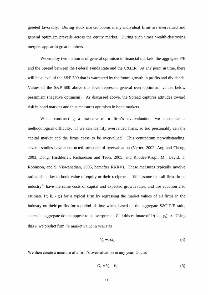
The first column in Table 1 presents the total numbers of mergers and acquisitions

(M&As) in our sample from 1985 to 2008. Consistent with Figure 1, the number of

transactions increases steadily from 1985 to 2000 (with a slight decline in 1999). A relatively

18

dormant period can be observed over 2001-2003. M&A activity increases again to high

levels over the 2004-2007 period and declines in 2008.

The second column in Table 1 reports the average values of our measures of

overvaluation deflated by company total assets for the acquiring companies in our sample.

They begin negative and rise during the first wave peaking at a value of 1.67 in 1999. Thus,

at the peak of the first merger wave, over half of the market value of an acquiring company

was, by our estimates, due to an overvaluation by the market. Average overvaluation falls

precipitously as the first merger wave ends reaching around 0.5 in 2002. It then rises again,

but does not regain the level reached at the peak of the first wave.

Our data source reports the fraction of each acquisition financed by issuing equity. It

attributes most of the rest of the finance of a merger to cash. This is misleading. When a

company wishes to finance a merger by issuing debt, it typically first sells bonds and then

uses the cash raised to finance the merger. To get a better estimate of the relative amounts of

debt and cash used to finance mergers we thus assumed that the proceeds from issuing debt

raised by a company making an acquisition in a given year were used to finance the merger,

so long as the amount of debt issued was not greater than the amount left to be financed after

taking account of the use of stock. Thus, if a company acquired another firm with a deal

value of $100 million, financed half of the acquisition by issuing equity, and also issued $40

million in bonds in the same year, we assume that the fraction financed by stock was 0.5, the

fraction financed by debt was 0.4, and the remaining 0.1 fraction was financed out of cash. If

this company had issued $60 million in debt in the year of the merger, we assume that the

fractions are: stock = 0.5, debt = 0.5, and cash = 0.

The last three columns of Table 1 report our estimates of the sources of finance for

mergers using this method of estimation starting in 1985, the first year for which we have

data. During the 1980s debt was the most preferred source of finance. These were the years

19

of the leveraged buyout, and the time when Michael Milken became famous and rich by

inventing the “junk bond.” Our estimates reflect the popularity of debt finance for mergers in

the 1980s. During the years of the first merger wave, the fractions of acquisitions financed

by issuing equity rose peaking at over 52 percent in 2000. In the second wave, however,

equity finance again gave way to debt for financing mergers with debt finance peaking in

2007 at over 50 percent.

The shifting importance of debt and equity as a means of finance for M&As revealed

in Table 1 suggests that any general theory of merger waves should be consistent with the use

of either source of finance at different points in time. We view this as another plus for the

managerial theory vis-à-vis the S&V overvaluation theory, which can only account for

mergers financed by issuing shares, since it is only equity that is assumed to be overvalued.

Our hypotheses predict the signs on the relevant variables, but not the functional form

of the relationship. We experimented with polynomials up to the third order, but report

results for the higher order terms, only when they are significant. The models are estimated

using the Tobit procedure, since we postulate that they explain not only whether or not a

company makes an acquisition, but also the acquisition’s size. More discretion leads

managers to undertake bigger mergers. Results from probit regressions differed from the

Tobit results only with respect to the sizes of the variables’ coefficients – the same variables

that explain whether or not a firm undertakes a merger explain the amount of assets acquired.

The close similarity between the probit and Tobit results also implies that there was little to

gain from adopting Heckman’s (1976) two-stage estimation procedure for censored data.

Here it is perhaps also worth reminding the reader that the two behavioral hypotheses

are not assumed to explain all mergers, but rather the increases in mergers during stock

market booms. The error term in the model can be assumed, therefore, to capture other

causes of mergers that are not part of the two behavioral hypotheses.

20

Summary statistics are presented in Table 2a. The variables are as follows. DV is the

deal value, the total consideration paid by the acquirer excluding fees and expenses. We

divide DV by the total assets of the acquirer and call this variable Assets Acquired. Tobin’s q

is a firm’s market value divided by its total assets. Market value is the sum of the market

value of its common stock, the book values of total short and long term debt (9+34,

Compustat numbers for the items appear in parentheses), and preferred stock, defined as

available, as redemption value (56), liquidating value (10), or par value (130). The market

value of common stock is the end-of-fiscal year number of shares (54) times end-of-fiscal

year share price (199). Leverage, L, is the ratio of total debt to total assets. Cash flow, CF, is

after tax profits before extraordinary items (18) plus depreciation (14). All variables are

deflated by the CPI (1985=1.00).

The average deal value was $359.5 million. This corresponds to almost 25 percent of

the total assets of the acquiring company in the average transaction. Acquiring companies

are larger than companies in our control group (with total assets amounting to almost $3.6

billion versus $1.2 billion). Mean Tobin’s q for acquirers is equal to 1.95, and is slightly

lower than the average q for the control group (2.13). Acquirers have higher levels of cash

flows than non-acquirers, and their average is slightly higher than for the control group.

Table 2b presents correlation coefficients for the main variables. Assets acquired are

significantly positively correlated with q, OV/TA, P/E, and significantly negatively

correlated with the spread, S, cash flows and leverage. Tobin’s q is highly correlated with

overvaluation as expected, r = 0.95. Somewhat unexpectedly, q is negatively correlated with

cash flows. It also has large negative correlations with company size and leverage.

VI. Results of the Tests

A. The Determinants of Mergers

21

The first equation in Table 3 presents the results for the basic, determinants model.

The three key variables of the behavioral theories – the P/E, Spread, and overvaluation – are

all highly significant with the predicted signs.19

Leverage and log size are also highly

significant. Highly levered firms tend to acquire fewer assets. The positive coefficient on

size can be regarded as support for the managerial theory, under the assumption that large

size offers more protection to managers undertaking wealth destroying mergers. Cash flow is

also highly significant with the predicted positive coefficient.

The second equation in Table 3 adds the Federal Funds Rate. Its coefficient is

negative and significant as expected, if it acts as a measure of borrowing costs. As noted

above, the coefficient on Spread should be equal to that on FF, if Spread was also serving

solely as a measure of borrowing costs. Spread’s coefficient is twelve times that of FF (in

absolute terms), however, indicating that Spread measures something different, like optimism

in the bond market. The signs and significance of the other variables in the model are

unaffected by the addition of the Federal Funds Rate. The results in Table 3 indicate that

significantly more assets are acquired when optimism in both the bond and stock markets is

high, and that firms with overvalued shares acquire significantly more assets than companies

with correctly priced shares.

B. The Determinants of the Means of Finance

Table 4 reports the estimated coefficients of equation 8. As predicted, optimism in

the equity market, as measured by the aggregate P/E ratio, is associated with greater reliance

on the use of equity to finance mergers, and high borrowing costs, C&ILR, also lead

managers to prefer equity to debt. Firm specific optimism as measured by the ratio of

overvaluation to total assets, OV/TA, is also highly significant with the predicted sign.

22

We obtain a significantly positive coefficient on the size of the target relative to the

total assets of the acquirer, M/TA, which indicates that acquirers resort more heavily to

issuing equity to finance relatively large mergers. The coefficient on cash flow is negative as

predicted and highly significant. Companies with high cash flows rely on equity to a lesser

extent. Leverage also has a negative and significant coefficient, as it did in Table 3. Taken

together these two results imply that highly levered companies tend to acquire smaller

amounts of assets, and once they decide to merge they shy away from using equity,

reflecting the constraints they face in the financial markets.

The results in Table 4 confirm our hypothesis about the importance of optimism in the

stock market affecting the choice of finance for acquisitions. They might also be regarded as

consistent with the overvaluation theory. Overvalued companies favor the use of equity to

finance M&As. The results for cash flows and interest rates also meet expectations.

Companies with large cash flows use less equity to finance mergers, and high interest rates

lead to a greater use of equity.

C. The Effects of Market Optimism on Shareholder Returns

We expect the same measures of optimism within equity and bond markets and about

individual firms that determine the amount of assets that firms acquire through mergers to

also affect the success of the mergers. To test this prediction we first calculate the abnormal

returns to acquiring companies’ shareholders as the difference between the buy-and-hold

returns of acquirers and those of a control group, defined as non-acquiring firms belonging to

the same two-digit industry as the acquirer, which are of similar size (the same size-decile)

and of similar market-to-book ratio (same market-to-book decile). We estimated abnormal

returns for four windows – the month of the merger, and one, two and three years after the

merger. If the equity market is efficient, it should not be possible to predict the future

abnormal returns of a company. None of the variables we use to predict the abnormal returns

23

of acquirers should be significant. In fact all of them are when the abnormal returns are

estimated over the longer windows.

The inclusion of quadratic terms in the P/E and spread variables gave the best fit for

the one-, two- and three-year windows. We also included them in the equation estimated for

the one-month window, although none of the four variables was significant for this short

window (see Table 5, eq. 1). Indeed, only the overvaluation variable is significant for the

short window. This finding supports both of the behavioral theories. Under each, managers

expect that the market will not react unfavorably to the announcement of a merger, even

though the merger is not wealth-creating or even wealth-destroying. The fact that companies,

which are overvalued at the time they announce mergers, make higher returns at the

announcements indicates that the market’s (over)optimism persists, at least for a while, after

the mergers are announced.

The overvaluation variable continues to pick up a positive and significant coefficient

in the equation estimating one-year returns after the merger. It becomes negative and

significant, however, for the two- and three-year windows with the coefficient for the three-

year window more than double the size of the two-year coefficient. Thus, our results imply

that it takes the market more than a year after mergers are announced to begin to correct its

overvaluation of the acquirers at the merger announcements, and that the correction process

is continuing (at least) three years later.

Both the linear and quadratic terms for our two measures of market optimism are

significant and consistent with our hypotheses. The returns to acquirers’ shareholders fall as

optimism in the stock market at the time of the acquisitions, as measured by the

price/earnings ratio, rises. They also decline as optimism in the bond market grows (the

interest rate spread declines). The opposite signs on the squared terms for both of these

variables indicate that these effects taper off as optimism in the two markets increases. The

24

implied differences in returns to acquirers are large. After one year, acquirers earn 7 percent

lower abnormal returns when the P/E is 30 at the time of an acquisition than when it is 15.

After 2 or 3 years, the difference is around 30 percent. The negative coefficients on

overvaluation for the two- and three-year windows indicate that some of the wealth loss to

acquiring companies’ shareholders following mergers is due to the market’s correction of its

overvaluation of them at the time of the mergers. The significant coefficients on the P/E and

spread reveal, however, that overvaluation of acquirers does not account for all of the wealth

losses to acquirers’ shareholders. Mergers when optimism in the stock and bond markets is

high result in wealth losses to acquirers’ shareholders over and above any market corrections

of firm-specific overvaluation.

We saw in Table 3 that highly levered firms tend to be less active in the M&A

market. The results in Table 5 indicate that when highly levered firms do undertake a

merger, they are more successful than less levered acquirers.

VII. Conclusions

Three prominent “stylized facts” about mergers in the United States are that they

come in waves, the crests of the waves are associated with stock market rallies, and the

shareholders of acquiring companies suffer significant wealth losses over long post-merger

windows from mergers undertaken during merger waves. This article explains the links

among these three phenomena by emphasizing the importance of optimism. Optimism in

financial markets drives share prices and price/earnings ratios to levels that are unsustainable

at historic growth rates. Aggressive managers take advantage of the market’s optimism to

undertake unprofitable mergers. Mergers that in normal times would be met with sharp share

price declines are greeted more favorably, because of the market’s optimism. We have

presented evidence that the amount of assets acquired by companies increases with increasing

25

optimism in both the equity and bond markets. Individual companies that are overvalued

also engage in more M&A activity than other firms.

During the merger wave at the end of the 20th

century, when optimism in the equity

market and company overvaluations were at record highs, the favored source of finance for

mergers was equity. During the 1980s, however, issuing debt to raise cash to finance

mergers was more common. The same was true during the merger wave of the 1960s, when

the companies that became “conglomerates” through unrelated acquisitions expanded their

debt by far greater amounts than companies that were less active in acquiring other firms

(Weston and Mansinghka, 1971). New debt was also preferred to new equity during the

merger wave from 2004 to 2008. This was a period of low interest rates and, by our measure,

high optimism in debt markets. These developments fueled not only this merger wave, but,

of course, speculation in the housing market, and eventually produced the financial crisis and

a collapse in housing prices and M&A activity. Our models of assets acquired through

mergers and the choice of finance illuminate the links among these developments.

Additional evidence for the managerial theory of mergers was provided by the model

to explain abnormal returns to acquiring companies. Mergers undertaken when optimism in

equity and bond markets is high are followed by significantly lower returns to shareholders of

acquiring companies than for mergers undertaken in more normal times. Thus, our results

demonstrate that optimism in financial markets explains the amount of assets acquired

through mergers at different points in time, the means for financing them, and the returns to

the acquirers’ shareholders following the mergers.

These findings are inconsistent with recent “neoclassical” theories of merger waves.

These theories assume that capital markets are efficient and thus, by assumption, rule out

over optimism in financial markets and the overvaluation of individual companies as causes

26

of mergers and merger waves. Our findings of negative returns to acquirers’ shareholders are

also inconsistent with the assumption that managers maximize shareholder wealth.

Some of our findings are consistent with the S&V overvaluation theory of mergers.

Company overvaluations are positively related to assets acquired, and negatively related to

post-merger returns after two and three years. An advantage of the managerial theory over

the overvaluation theory is, however, that it can also account for mergers financed by debt or

cash. We also show that the wealth losses to acquirers are greater not only for firms that are

overvalued, but also when there is optimism in the equity and bond markets – the key

determinants of mergers under the managerial theory.

The wealth destruction following mergers can be quite large. Moeller, Schlingemann,

and Stulz (2005) estimated abnormal returns to acquirers during the 1998-2001 merger wave

of -12 percent, producing a wealth loss to acquirers of some $240 billion. For the two merger

waves that we cover the average abnormal returns to acquirers after two years were almost

-18 percent. Moreover, it is not only the shareholders of acquirers who suffer from bad

mergers. The entire economy suffers to the extent that managers in the pursuit of growth

through mergers avoid other avenues of growth like R&D and innovations that have positive

social benefits.

27

References:

Agrawal, Anup and Jeffrey F. Jaffe. (2000). “The Post-Merger Performance Puzzle.” in

Advances in Mergers and Acquisitions, 1, Amsterdam: Elsevier, 7-41.

Agrawal, Anup, Jeffrey F. Jaffe and G. N. Mandelker. (1992). “The Post-Merger

Performance of Acquiring Firms: A Re-examination of an Anomaly.”Journal of

Finance, 47(4), 1605-21.

Andrade, Gregor, and Erik Stafford. (2004). “Investigating the Economic Role of Mergers.”

Journal of Corporate Finance, 10, 1-36.

Ang, J. and Y. Cheng. (2003). “Direct Evidence on Stock Market Driven Acquisitions

Theory.”Florida University Working Paper.

Asquith, Paul. (1983). “Merger Bids, Uncertainty, and Stockholder Returns.”Journal of

Financial Economics, 11 (1-4), 51-83

Barsky, Robert and Bradford De Long. (1993). “Why Does Stock market Fluctuate?”

Quarterly Journal of Economics, 108(2), 291-311.

Becher, D. (2000). “The Valuation Effects of Bank Mergers.” Journal of Corporate Finance,

6, 189–214.

Bhagat, Sanjai, Dong, Ming, Hirshleifer, David and Robert Noah. (2005). “Do Tender Offers

Create -Value? New Methods and Evidence.” Journal of Financial Economics, 76(1),

3-60.

Bhagat, Sanjay, Andrei Shleifer and Robert W. Vishny. (1990). "Hostile Takeovers in the

1980s: The Return to Corporate Specialization." Brookings Papers on Economic

Activity, 1-84.

Bliss, R. T. and R. J. Rosen (2001). “CEO Compensation and Bank Mergers.” Journal of

Financial Economics, 61, 107-38.

Bradley, M., Desai, A. and E.H. Kim. (1988). “Synergistic Gains from Corporate

Acquisitions and Their Division between the Stockholders of Target and Acquiring

Firms.” Journal of Financial Economics, 21(1), 3-40.

Caves, R. E. (1989). “Mergers, Takeovers, and Economic Efficiency.” International Journal

of Industrial Organization, 7, 151-174.

28

Chappell, H. W. and D. C. Cheng. (1984). Firms, Acquisition Decisions and Tobin’s q

Ratio,” Journal of Economics and Business, 36, 29-42.

Clarke, Roger and Christos Ioannidis. (1996). “On the Relationship between Aggregate

Merger Activity and the Stock Market: Some Further Empirical Evidence.”

Economics Letters, 53: 349-356.

Damodaran, Aswath. (2005). “Estimating Equity Risk Premiums.” Working Paper, Stern

School of Business.

Datta, Deepak K., George E. Pinches and V.K. Narayanan. (1992). “Factors Influencing

Wealth Creation From Mergers and Acquisitions: A Meta Analysis.” Strategic

Management Journal, 13, 67-84.

Denis Debra K. and John J. McConnell. (1986). “Corporate Mergers and Security Returns.”

Journal of Financial Economics, 16, 143-87.

Dodd, Peter and Richard Ruback. (1977). “Tender Offers and Stockholder Returns: An

Empirical Analysis.” Journal of Financial Economics, 5, 351-74.

Dong, Ming, David Hirschleifer, Scott Richardson, Siew Hong Teoh. (forthcoming). “Does

Investor Misvaluation Drive the Takeover Market?” Journal of Finance.

Doukas, John. (1995). “Overinvestment, Tobin's Q and Gains from Foreign Acquisitions.”

Journal of Banking and Finance, 19, 1285-1303

Eckbo, Espen and Karin S. Thorburn. (2000). “Gains to Bidder Firms Revisited: Domestic

and Foreign Acquisitions in Canada.” Journal of Financial and Quantitative Analysis

35, 1-25.

Economist. (1991). “A Survey of International Finance (From Morgan’s Nose to Milken’s

Wig).” April 27th

.

Economist. (2000). “How Mergers Go Wrong”, July 20th

.

Economist. (2005). “Love is in the Air.” February 3rd

.

Ellert, James. (1976). “Mergers, Antitrust Law Enforcement and Stockholder Returns.”

Journal of Finance, 31, 2, 715-732.

Erard, B. and H. Schaller. (2002). “Acquisitions and Investment.” Economica, 69, 391-414.

29

Fama, Eugene and Kenneth French. (1997). “Industry Costs of Equity.” Journal of Financial

Economics 43, 153–193.

Fama, Eugene. (1998). “Market Efficiency, Long-Term Returns and Behavioral Finance.”

Journal of Financial Economics 49, 283-306.

Fisher, A. B. (1984). “The Decade's Worst Mergers.” Fortune, April 30, 1984, pp. 262- 270.

Geroski, Paul A. (1984). “On the Relationship between Aggregate Merger Activity and the

Stock Market.” European Economic Review, 25, 223-33.

Golbe, Devra L., and Lawrence J White. (1993). “Catch a Wave: The Time Series Behavior

of Mergers.” The Review of Economics and Statistics, 75, 493-499.

Grabowski, Henry and Dennis C. Mueller. (1972). “Managerial and Stockholder Welfare

Models of Firm Expenditures.” Review of Economics and Statistics 54, 9-24.

Gregory, A. (1997). “An Examination of the Long Run Performance of UK Acquiring

Firms.” Journal of Business Finance and Accounting, 24, 971-1002.

Gugler, Klaus, Dennis C. Mueller and B. Burcin Yurtoglu (2005). “Tests of Neoclassical

Theories of Merger Waves.” Working Paper, University of Vienna.

Gugler, Klaus, Dennis. C. Mueller and B.Burcin Yurtoglu. (2004). “Marginal q, Average q,

Cash Flow and Investment.” Southern Economic Journal, 70, 512–531.

Harford, Jarrod (2005). “What Drives Merger Waves?” Journal of Financial Economics,

Journal of Financial Economics, 77(3), 529-560.

Harford, Jarrod. (1999). “Corporate Cash Reserves and Acquisitions.” Journal of Finance,

54, 1969-97.

Harford, Jarrod and K. Li. (2007). “Decoupling CEO Wealth and Firm Performance: The

Case of Acquiring CEOs.” Journal of Finance, 62, 917-49.

Hay, Donald A. and Guy S Liu. (1998). “When Do Firms Go in for Growth by

Acquisitions?”Oxford Bulletin of Economics and Statistics, 60(2), 143-64.

Heckman, J. (1976). “The Common Structure of Statistical Models of Truncation, Sample

Selection, and Limited Dependent Variables and a Simple Estimator for such

Models.” The Annals of Economic and Social Measurement 5: 475-492.

30

Higson, C. and J. Elliott. (1998). “Post-takeover Returns: The UK Evidence.” Journal of

Empirical Finance, 5 (1), 27-46.

Houston J.F. and M.D. Ryngaert. (1994). “The Overall Gains from Large Bank Mergers.”

Journal of Banking and Finance, 18 (6), 1155-1176

Hubbard, Robert Glenn and Darius Palia. (1995). “Benefits of Control, Managerial

Ownership, and the Stock Returns of Acquiring Firms.” Rand Journal of Economics,

26, 782-792.

Jarrell Gregg. A and A. B. Poulsen. (1989). “The Returns to Acquiring Firms in Tender

Offers: The Empirical Evidence since 1980.” Financial Management, 18, 371-407.

Jarrell, Gregg. A., James A. Brickley and Jeffrey M. Netter. (1988). “The Market for

Corporate Control: The Empirical Evidence Since 1980.” Journal of Economic

Perspectives, 2(1), 49-68.

Jensen, Michael C. and R.S. Ruback. (1983). “The Market for Corporate Control: The

Scientific Evidence.” Journal of Financial Economics, 11, 5-50.

Jovanovic Boyan and Peter L. Rousseau. (2002). “The Q-Theory of Mergers.” American

Economic Review Papers and Proceedings, May, 198-204.

Kang, Jun-Koo. (1993). “The International Market for Corporate Control: Mergers and

Acquisitions of U.S. Firms by Japanese Firms.” Journal of Financial Economics, 34,

345-71.

Khorana, Ajay and Marc Zenner. (1998). “Executive Compensation of Large Acquirors in the

1980s.” Journal of Corporate Finance, 4, 209-240.

Lang, Larry H. P., René M. Stulz and Ralph Walking. (1989). “Managerial Performance,

Tobin's q, and the Gains from Successful Tender Offers.” Journal of Financial

Economics 24, 137-54.

Langetieg, T. (1978). “An Application of a Three-Factor Performance Index to Measure

Stockholder Gains from Merger.” Journal of Financial Economics 6, 365-384.

LeRoy and Porter (1981). “The Present-Value Relation: Tests Based on Implied Variance

Bounds.” Econometrica, 27, 555-74.

LeRoy, Stephen. (1989). “Efficient Capital Markets and Martingales.” Journal of Economic

Literature, 27, 1583-1622.

31

Linn, Scott C. and Zhen Zhu. (1997). “Aggregate Merger Activity: New Evidence on the

Wave Hypothesis.” Southern Economic Journal, 64, 130-46.

Lintner, John. (1971). “Expectations, Mergers and Equilibrium in Purely Competitive

Securities Markets.” American Economic Review, 61, 101-11.

Loderer, Claudio and K. Martin. (1997). “Executive Stock Ownership and Performance:

Tracking Faint Traces.” Journal of Financial Economics 45 (2), 223-255.

Magenheim, Ellen B. and Dennis C. Mueller. (1987). “On Measuring the Effect of

Acquisitions on Acquiring Firm Shareholders, or are Acquiring Firm Shareholders

Better off after an Acquisition Than They Were Before?” in John C. Coffee, Jr., Louis

Lowenstein, and Susan Rose-Ackerman, eds., Takeovers and Contests for Corporate

Control, Oxford: Oxford University Press, 171-93.

Malatesta, P.H. (1983). “The Wealth Effect of Merger Activity and the Objective Functions

of Merging Firms.” Journal of Financial Economics, 11, 155-81.

Mandelker, G., (1974). “Risk and Return: The Case of Merging Firms.” Journal of Financial

Economics, 1, December, 303-35.

Manne, Henry G. (1965). “Mergers and the Market for Corporate Control.” Journal of

Political Economy, 73, 110-120.

Maquieira, Carlos P., William L. Megginson and Nail, Lance. (1998). “Wealth Creation

versus Wealth Redistributions in Pure Stock-for-Stock Mergers.” Journal of

Financial Economics, 48(1), 3-33.

Markham, Jesse W. (1955). “Survey of the Evidence and Findings on Mergers.” in Business

Concentration and Price Policy, N.B.E.R., Princeton University Press, Princeton.

Marris, Robin. (1963). “A Model of the ‘Managerial’ Enterprise.” Quarterly Journal of

Economics, 77, 185-209.

Marris, Robin. (1964). The Economic Theory of Managerial Capitalism, Glencoe: Free Press.

Marris, Robin. (1998). Managerial Capitalism in Retrospect. Palgrave-Macmillan, London.

Mead, W. J. (1969). “Instantaneous Merger Profit as Conglomerate Merger Motive,” Western

Economic Journal, 7, 295-306.

Melicher, R. W., J. Ledolter, and L. J. D’Antonio. (1983). “A Time Series Analysis of

Aggregate Merger Activity.” Review of Economics and Statistics 65, 423-430.

32

Melicher, Ronald W. and David F. Rush. (1973). “The Performance of Conglomerate Firms:

Recent Risk and Return Experience.” Journal of Finance, 28, 381-88.

Melicher, Ronald W. and David F. Rush. (1974). “Evidence on the Acquisition-Related

Performance of Conglomerate Firms.” Journal of Finance, 29, 141-49

Mitchell, M. L. and E. Stafford. (2000). “Managerial Decisions and Long-Term Stock

Performance.” Journal of Business 73, 287-320.

Mitchell, Mark L., and J. Harold Mulherin. (1996). “The Impact of Industry Shocks on

Takeover and Restructuring Activity.” Journal of Financial Economics, 41(2), 193-

229.

Moeller, Sara B., Frederik P. Schlingemann and René M. Stulz. (2005). “Wealth Destruction

on a Massive Scale? A Study of Acquiring-Firm Returns in the Recent Merger

Wave.” Journal of Finance, 60 (2), 757-782.

Mueller, Dennis C. (1969). “A Theory of Conglomerate Mergers.” Quarterly Journal of

Economics, 83, November, 643-59.

Mueller, Dennis C. (1977). "The Effects of Conglomerate Mergers: A Survey of the

Empirical Evidence," Journal of Banking and Finance, 1, 315-47. Reprinted in

Cheng-few Lee, ed., Financial Analysis and Planning: Theory and Application, A

Book of Readings, Reading, Mass.: Addison-Wesley, 1983, pp. 450-82. Reprinted in

G. Marchildon, ed., Mergers and Acquisitions, London: Edward Elgar, 1991.

Mueller, Dennis C. (2003). The Corporation: Investment, Mergers, and Growth, Routledge,

London.

Mueller, Dennis C. and Mark L. Sirower. (2003). “The Causes of Mergers: Tests Based on

the Gains to Acquiring Firms' Shareholders and the Size of Premia.” Managerial and

Decision Economics, 24 (5), 373-416.

Mulherin, J.H. and A. Boone. (2000). “Comparing Acquisitions and Divestitures.” Journal of

Corporate Finance 6, 117-139.

Nelson, Ralph, L. (1959). Merger Movements in American Industry, 1895-1956, Princeton:

Princeton University Press.

33

Nelson, Ralph L. (1966). “Business Cycle Factors in the Choice Between Internal and

External Growth.” in W. Alberts and J. Segall, eds., The Corporate Merger, Chicago:

University of Chicago Press.

Pautler, Paul A. (2003). “Evidence on Mergers and Acquisitions.” The Antitrust Bulletin,

Spring, 48 (1), 119-221.

Perfect, S.B. and K.W. Wiles. (1994). “Alternative Constructions of Tobin's q: An Empirical

Comparison.” Journal of Empirical Finance, 1, 313-341.

Philippatos, George C. and Philip L. Baird, III. (1996). “Postmerger Performance,

Managerial Superiority and the Market for Corporate Control.” Managerial and

Decision Economics, 17, 45-55.

Rau, R., and Theo Vermaelen. (1998). “Glamour, Value and the Post-acquisition

Performance of Acquiring Firms.” Journal of Financial Economics, 49, 223-253.

Resende, Marcelo. (1999). “Wave Behaviour of Mergers and Acquisitions in the UK: A

Sectoral Study.” Oxford Bulletin of Economics and Statistics, 61(1), 85-94.

Rhodes-Kropf, M. and S. Viswanathan. (2004). “Market Valuation and Merger Waves.”

Journal of Finance, 59, 2685–2718.

Rhodes-Kropf, M., David. T. Robinson, and S. Viswanathan. (2005). “Valuation Waves and

Merger Activity: The Empirical Evidence.” Journal of Financial Economics, 77 (3),

561-603.

Roe, Mark J. (1993). “Takeover Politics.” in: Margaret M. Blair (Ed.) The Deal Decade, The

Brookings Institution, Washington, D.C.

Röller, Lars-Hendrik, Johan Stennek and Frank Verboven. (2001). “Efficiency Gains from

Mergers.” European Economy, 5, 31-128.

Scherer, F.M. and David Ross. (1990). Industrial Market Structure and Economic

Performance, 3rd ed., Boston: Houghton Mifflin.

Schwartz, S. (1984). “An Empirical Test of A Managerial, Life-Cycle, and Cost of Capital

Model of Merger Activity.” Journal of Industrial Economics, 32(3), 265-75.

Schwert, G.W. (2000). “Hostility in Takeovers: In the Eyes of the Beholder?” Journal of

Finance, 55 (6), 2599-2640.

34

Schwert, William G. (1996). “Markup Pricing in Mergers and Acquisitions.” Journal of

Financial Economics, 153-192.

Shiller, Robert J. (1981). "Do Stock Prices Move Too Much to be Justified by Subsequent

Changes in Dividends?" American Economic Review, 71(3), 421-36.

Shiller, Robert J. (2000). Irrational Exuberance, Princeton: Princeton University Press.

Shleifer, Andrei. (2000). Inefficient Markets: An Introduction to Behavioral Finance, Oxford:

Oxford University Press.

Shleifer, Andrei and Robert W. Vishny. (2003). “Stock Market Driven Acquisitions.”

Journal of Financial Economics, 70 (3), 295-489.

Smith, Richard, and Kim, Joo-Hyun. (1994). “The Combined Effects of Free Cash Flow and

Financial Slack on Bidder and Target Stock Returns.” Journal of Business 67, 281-

310.

Steiner, P. O. (1975). Mergers: Motives, Effects, Control, Ann Arbor: University of Michigan

Press.

Summers, Lawrence. (1986). “Does the Stock Market Rationally Reflect Fundamental

Values?” Journal of Finance, 41(3), 591-601.

Thaler, Richard H. (1991). Quasi-Rational Economics, New York: Russell Sage Foundation.

Thaler, Richard H., ed. (1993). Advances in Behavioral Finance, New York: Russell Sage

Foundation.

Verter, Geoffrey . (2002). “Timing Merger Waves.” Working Paper, Harvard University.

Vogt, S. C. (1994). “The Cash Flow/Investment Relationship: Evidence from U.S.

Manufacturing Firms.” Financial Management, 23, 3-20.

Weston, J. Fred and S. K. Mansinghka. (1971). “Tests of the Efficiency Performance of

Conglomerate Firms.” Journal of Finance, 26(Sept.), 919-36.

Wooldridge, J. M. (2002). “Econometric Analysis of Cross Section and Panel Data”, MIT

Press.

Zweig, Phillip L. (1995). “The Case Against Mergers.” Business Week (October 30), 122-30.

35

Figure 1: M&A and P/E

Sources: DV is total deal values of Mergers and Acquisitions per month, in Million USD. The data are from SDC database. The figure shows a 3-month moving average. S&P

P/E is the monthly price-earnings ratio for the S&P 500 index. It is provided by Robert Shiller (http://www.econ.yale.edu/~shiller/data.htm).

36

Figure 2: M&A, real Commercial and Industrial Loan Rate (C&ILR), and Spread

Sources: DV is total deal values of Mergers and Acquisitions per month, in Million USD. The data are from SDC database. Real C&ILR is the CPI-inflation-adjusted

Commercial and Industrial Loan Rate. Spread is the difference between C&ILR and the Federal Funds Rate. Spread and C&ILR are from http://www.federalreserve.gov.

37

Figure 3: The managerial trade-off

38

Table 1: Number of M&A, Overvaluation and Means of Finance

Means of Finance

M&A O/TA Stock Debt Cash

1985 68 0.056 0.192 0.651 0.157

1986 154 0.086 0.224 0.553 0.223

1987 146 -0.163 0.410 0.377 0.213

1988 183 -0.075 0.229 0.564 0.207

1989 252 0.068 0.307 0.450 0.243

1990 261 -0.132 0.387 0.398 0.214

1991 314 0.481 0.416 0.345 0.239

1992 411 0.515 0.402 0.379 0.219

1993 472 0.572 0.381 0.376 0.243

1994 583 0.267 0.358 0.464 0.177

1995 634 0.585 0.433 0.390 0.177

1996 806 0.622 0.429 0.365 0.206

1997 939 0.781 0.406 0.397 0.197

1998 1,070 0.822 0.400 0.428 0.172

1999 1,011 1.665 0.465 0.366 0.169

2000 1,017 0.772 0.523 0.306 0.170

2001 850 0.847 0.435 0.320 0.245

2002 803 0.534 0.279 0.417 0.304

2003 847 1.460 0.285 0.440 0.274

2004 1,038 1.435 0.226 0.468 0.306

2005 1,171 1.216 0.238 0.453 0.309

2006 1,264 1.279 0.207 0.486 0.307

2007 1,224 1.236 0.211 0.506 0.283

2008 979 0.338 0.169 0.458 0.373

Total 16,497 0.636 0.334 0.432 0.234

Note: The number of mergers and acquisitions is from the SDC database and includes all transaction where

more than 50 percent of the target’s equity is acquired. O is overvaluation as described in section IV. A. (see

equation (5)). O/TA is overvaluation relative to the total assets of the firm. Stock refers to the average fraction

of the deal value paid in shares, Debt refers to the average fraction of the deal value financed by debt. Cash

refers to the average fraction of the deal value paid in cash.

39

Table 2a: Summary statistics, mean values

Acquirers Controls

Deal Value (DV, Thsd USD) 359,515

Assets Acquired (DV/TA) 0.247

Total Assets (TA, Thsd USD) 3,656,185 1,266,801

ln(TA) 12.68 11.18

Tobin's q 1.95 2.13

Cash Flow (CF/TA) 0.0769 0.0565

Leverage 0.26 0.24

N 10,729 50,495

Note: Only firm years with deals are used to calculate mean values for acquirers. Cash Flow is net income plus

depreciation divided by total assets (TA). Leverage is the ratio of total debt to total assets. Overvaluation is Oit

from equation (5) expressed as a fraction of market value (O/MV). DV is the deal value (i.e. the total amount

paid for the target). Assets acquired is the Deal Value divided by total assets.

Table 2b: Correlation Coefficients

Assets A. O P/E S ln(TA) CF L q

O 0.061 1

0.000

P/E 0.066 0.082 1

0.000 0.000

S -0.026 0.030 -0.124 1

0.000 0.000 0.000

ln(TA) -0.008 -0.322 -0.032 0.056 1

0.049 0.000 0.000 0.000

CF -0.023 -0.378 -0.049 -0.076 0.393 1

0.000 0.000 0.000 0.000 0.000

L -0.014 -0.121 -0.014 0.013 0.339 0.044 1

0.000 0.000 0.001 0.001 0.000 0.000

q 0.057 0.951 0.072 0.022 -0.302 -0.342 -0.127 1

0.000 0.000 0.000 0.000 0.000 0.000 0.000

FF 0.010 -0.050 0.069 -0.706 -0.039 0.066 -0.004 -0.040

0.010 0.000 0.000 0.000 0.000 0.000 0.370 0.000

Note: Only firm years with deals are used to calculate mean values for acquirers. Cash Flow (CF) is net income

plus depreciation divided by total assets (TA). Leverage is the ratio of total debt to total assets. Overvaluation is

itO from equation (5) expressed as a fraction of the total assets (O/TA). DV is the deal value (i.e. the total

amount paid for the target). Assets acquired is the Deal Value divided by total assets. P/E is the value of the

Standard and Poor’s 500 price-earnings ratio. S is the spread between the Federal Funds Rate (FF) and the

Commercial & Industrial Loan Rate. The p-values are reported below the correlation coefficients.

40

Table 3: Explaining the Amounts of Assets Acquired

Table 3 reports the Tobit estimates of the coefficients of Eq. 6 and Eq. 7. The dependent variable is the Assets

acquired (Deal Value divided by total assets). Overvaluation (O) is Oit from equation (5) expressed as a fraction

of total assets. P/E is the value of the Standard and Poor’s 500 price-earnings ratio. S is the spread between the

Federal Funds Rate (FF) and the Commercial & Industrial Loan Rate. Ln(TA) is the natural logarithm of total

assets. Cash Flow (CF) is net income plus depreciation divided by total assets (TA). Leverage (L) is the ratio of

total debt to total assets. Industry dummies according to the SIC (2-digit) are included and the table shows the F-

test result for being jointly different from zero. Acquirers are excluded from the control group two years before

and two years after the deal.

(6) (7)

Coeff. (t-value) Coeff. (t-value)

O 0.0183 (12.8) 0.0180 (12.6)

P/E 0.0092 (19.8) 0.0093 (19.9)

S -0.1200 (-9.4) -0.2018 (-11.5)

ln(TA) 0.0799 (43.6) 0.0796 (43.4)

CF 0.1165 (6.0) 0.1190 (6.1)

L -0.0501 (-3.1) -0.0501 (-3.1)

FF -0.0168 (-6.9)

constant -1.0900 -(8.6) -1.0367 (-20.5)

Industry dummies F(67, 44,962) = 23.1 F(67, 44,961) = 23.0

N (Mit>0) 45,035 (10,465) 45,035 (10,465)

R2 0.1108 0.1119

41

Table 4: Explaining the Choice of Finance

Table 4 presents the Tobit estimates of the coefficients of equation 8. The dependent variable is EFit, the fraction

of assets acquired by i in t by issuing new shares. C&ILR is the Commercial and Industrial Loan Rate (from

http://www.federalreserve.gov/releases/E2/e2chart.htm). M is the size of the target relative to total assets of the

acquirer. The remaining variables are defined in the notes to Table 3.

(8)

Coeff. (t-value)

O 0.088 (9.2)

P/E 0.018 (6.8)

C&ILR 0.093 (8.1)

M 0.949 (18.4)

CF -1.099 (-10.6)

L -0.631 (-7.8)

constant -1.384 (-14.2)

N 7,681

R2 0.0800

42

Table 5: Explaining Abnormal Returns

Table 5 shows the estimates for equation 9 for the cases of abnormal returns after one month, one, two and three

years after the merger announcement date. The average abnormal returns for acquirers for the four windows are

calculated against a control group of all companies which did not make an acquisition in the year prior to the

month of the acquisition and over the length of the window, i.e. ,,

noningi t ti tAR R R . where ,i tAR is the

abnormal return of acquiring firm i during period t; ,ing

i tR is the total return of acquiring firm i during period t,

and non

tR is the average total return of all non-acquiring firms during period t. We use the total return index

from Datastream, which is adjusted for dividend payments and share splits. The explanatory variables are

defined as in Table 3. P/E2 and S

2 are P/E squared and S squared, respectively.

(9) 1 month (9) 1 year (9) 2 years (9) 3 years

Coef. t-value Coef. t-value Coef. t-value Coef. t-value

P/E -0.0004 (-0.4) -0.0162 (-4.1) -0.0720 (-12.0) -0.0902 (-11.6)

P/E2 0.0000 (-0.4) 0.0002 (3.0) 0.0012 (11.6) 0.0016 (12.1)

S -0.0064 (-0.2) 0.5894 (2.5) 2.2546 (6.2) 1.9370 (4.1)

S2 0.0047 (0.5) -0.2114 (-3.6) -0.6479 (-7.4) -0.6147 (-5.4)

O 0.0010 (2.1) 0.0044 (2.4) -0.0165 (-5.8) -0.0324 (-8.9)

L 0.0065 (1.5) 0.0863 (4.8) 0.1678 (6.1) 0.2345 (6.6)

constant 0.0086 (0.2) -0.0958 (-0.4) -0.9361 (-2.4) -0.3018 (-0.6)

N 15,001 14,350 13,315 12,248

R2 0.003 0.0263 0.0489 0.0677

43

Notes: 1 Ralph Nelson (1959, 1966) was the first to document the link between merger activity and share

prices, and numerous subsequent studies have confirmed this finding. See, for example, Melicher,

Ledolter and D’Antonio (1983), Geroski (1984) for the US, and Geroski (1984) and Clarke and

Ioannidis (1996) for the UK.

2 Shiller’s index is constructed from P/E data for the S&P 500 (see Shiller, 2000, and the data section

on his webpage, http://www.econ.yale.edu/~shiller). A very similar pattern exists if we substitute the

Dow Jones Industrials Index or the S&P 500 Index.

3 For surveys of this literature, see Steiner (1975), Scherer and Ross (1990, pp. 153-198), Mueller

(2003, ch. 8), Weston, Chung and Hoag (1990), and Röller, Stennek and Verboven (2001), and

Pautler (2003).

4 See the survey by Jensen and Ruback (1983).

5 See, Thaler (1991, 1993) and Shleifer (2000). 6 For additional evidence see, LeRoy and Porter (1981), Summers (1986), Barsky and De Long

(1993). LeRoy (1989) offers a survey.

7 See, Damodaran (2005).

8 For an account of the hypothesis by an academic, see Mead (1969).

9 Several studies have traced the relative performance of the conglomerates during and after the stock

market boom of the 1960s. See, for example, Melicher and Rush (1973, 1974). We discuss

additional evidence below based on share performance over long windows.

10 When testing his industry shocks theory of merger waves, Harford (2005) uses the Spread as a

measure of the ease of financing mergers. This is partly an alternative interpretation of the variable,

partly an overlapping one. Borrowing funds may be more readily available due to greater optimism in

the bond market.

11 See, Khorana and Zenner (1998) and Harford and Li (2007).

12 A further justification for including q in the managers’ utility function would be that managers own

shares in the firm.

13 We assign each firm to one of the 48 industry groupings. These are the same groupings used by

Fama and French (1997) and by Harford (2005).

14 See, Grabowski and Mueller (1972), Vogt (1994), Hay and Liu (1998), and Gugler, Mueller and

Yurtoglu (2004).

15 For surveys, see Mueller (1977, 2003), Jensen and Ruback (1983), Jarrell, Brickley and Netter

(1988), Caves (1989), Jarrell and Poulsen (1989), Scherer and Ross (1990, pp. 167-174), Datta et al.

(1992) and Agrawal and Jaffee (2000).

16 This is generally true of the early literature reviewed in Jensen and Ruback (1983). More recent

studies reaching this conclusion include, Dennis and McConnell (1986), Bradley, Desai and Kim

(1988), Bhagat, Shleifer and Vishny (1990), Kang (1993), Doukas (1995), Bhagat, Hirshleifer and

Noah (2005), and Eckbo and Thorburn (2000).

17 See, for example, Lang, Stulz and Walking (1989), Houston and Ryngaert (1994), Smith and Kim

(1994), Hubbard and Palia (1995), Maquieira, Megginson and Nail (1998) and Becher (2000).

Moeller, Schlingemann and Stulz (2005), however, report huge short-run losses to acquirers for the

1990s merger wave.

18 For a discussion of why “friendly” mergers will be favored over hostile takeovers by managers

pursuing growth, see Mueller and Sirower, (2003). 19

Visual inspection of Figures 1 and 2 shows that some of our independent variables seem to be non-

stationary. However, because we are referring to a fixed-T, large-N asymptotics the time series

44

properties of the variables are irrelevant as long as our model is correctly specified. See for instance

Wooldridge (2002), p.175.