A theory of mergers and merger waves∗

Bingyong Zheng†

July 4, 2008

Abstract

We consider a model of horizontal mergers in a market consisting of Cournot firms pro-

ducing a homogeneous good with quadratic costs. High cost-savings froma merger or a

small slope for inverse market demand are both predicted to increase the incentive to merge.

The profitability of any merger is predicted to increase with the number of mergers having al-

ready taken place. Thus, an implication of this model is that mergers tend to occur in waves.

Another implication is that some mergers that are not profitable for the merged firms in the

short-run may take place in the early stage of a wave. The model helps to reconcile some of

the most important stylized facts about merger and acquisition activities in the USeconomy

over the last century.

Keywords: horizontal mergers; merger waves; Cournot oligopoly.

JEL classification codes: D43; L41.

1 Introduction

Mergers and acquisitions (M&A) in the US often occur in cyclical patterns: periods of intense

merger activity are followed by periods of relative calm. For example, 1998–2000 witnessed over

$1.5 trillion worth of announced deals each year while 2001 saw only half as much, as the dotcom

∗I am indebted to Al Slivinski for his help and suggestions at all stages of this project. I also thank Jimmy Chan

and Jacques Cremer for insightful comments. Of course, remaining errors are my own.†School of Economics, Shanghai University of Finance and Economics, 777 Guoding Rd., Shanghai, China

200433 Tel 86-21-6590-3124 Fax 86-21-6590-4198 E-mailbingyongzheng@yahoo.com.

era came to an end. After a short period of repose, nevertheless, M&A activities reached another

high in 2006; for the first time, the announced value of M&A reached $4 trillion in one year.1

The trend continued in mid-2007 until the subprime loan crisis in U.S. put an end to this wave.

Yet, the value of M&A in the first two quarters of 2007 still reached $2.7 trillion, 58% higher

than the first half of 2006.2 In this paper, we provide a simple model of horizontal mergers to

explain merger waves and related stylized facts from the empirical literature.

This literature (e.g.,Mitchell and Mulherin 1996, Andrade et al. 2001) has uncovered several

important facts about mergers and acquisitions over the 20th century. The first stylized fact is

the wave phenomenon mentioned above. Historians and M&A specialists have identified five

merger waves in the United States, not including the most recent flurry of M&A in 2006 to 2007.

These periods of intense merger activity are: 1897–1907; 1916–1929; 1965–1969;1981–1989;

and 1993–2000.

The second stylized fact identified by empirical studies is that mergers concentrate in indus-

tries that are subject to exogenous shocks. These shocks include: technological innovations;

supply shocks or changed market demand; and deregulation. The third stylized fact is that ac-

quirers’ returns are, on average, negative (seeBradley et al. 1988, Jennings and Mazzeo 1991,

Banerjee and Owers 1992, Byrd and Kickman 1992).3

These stylized facts are puzzling and hard to reconcile theoretically. Currently, there are two

1The Economist,Economic and financial indicators, Jan 23, 2007.2The Economist,Economic and financial indicators, Jul 7, 2007.3The statistical evidence on whether mergers create value for shareholders is based primarily on short-window

event studies. There are two frequently used event windows.The shorter one is from one day before to one day

after the announcement of merger, and the longer window begins several days before the announcement and ends at

the close of the merger. In a recent work,Andrade et al.(2001) have argued that the empirical finding of average

negative return could be due to negative stock market reaction to equity issue for acquisitions involving at least some

stock financing. According to them, stock financing mergers actually consist of two simultaneous transactions: a

merger and an equity issue. Various empirical studies have consistently shown that equity issue on average results

in negative abnormal returns of around -2 to -3 percent during the few days surrounding the announcement. Hence,

the finding of negative returns to acquirers on average couldbe a result of equity issuing as many mergers involve

some sort of stock financing. They then show that mergers solely financed by cash have average normal return that

is indistinguishable from zero.

2

approaches to explain the empirical findings: the behavioral approach and the neoclassical ap-

proach. To explain merger waves, theories following behavioral approach have assumed either

that the market is inefficient or that managers care about something other than firm profits. For

example, the managerial discretion hypothesis ofMorck, Schleifer, and Vishny(1990) attributes

mergers to managers’ self-interest or desire to manage a larger firm, while another hypothesis,

Gorton, Kahl, and Rosen(2005) argues that mergers occur as a defense again takeovers. Accord-

ing to Gorton et al., because larger size firms are less likely to be acquired, managers who prefer

their firms to stay independent have incentives to acquire smaller firms. The stock-market-driven

merger theory ofSchleifer and Vishny(2003) andRhodes-Kropf and Viswanathan(2004), on the

other hand, assumes that financial markets are not efficient.According to them, mergers and ac-

quisitions are driven by stock market overvaluations of merging firms. When some firms are

valued incorrectly in the market, rational managers can take advantage of the situation through

merger decisions.

While being able to explain the negative acquiring firms’ return, however, the behavioral

approach has difficulties explaining other empirical findings. First, why merger activities con-

centrated in industries exposed to the greatest exogenous shock? Second, how can the theories

explain mergers that are primarily financed by cash instead of stock? AsHarford(2005) points

out, the overvaluation hypothesis would predict that the method of payment in a wave should be

overwhelmingly stock. However, the fourth wave in 1981–1989 and the most recent merger activ-

ities in 2006 and 2007 are mainly debt-financed, which can notbe explained by the overvaluation

hypothesis.

In contrast with the behavioral approach, the neoclassicaltheories argue that mergers are

an efficient response to exogenous shocks by profit-maximizing managers. These studies (e.g.,

Mitchell and Mulherin 1996, Andrade et al. 2001, Andrade and Stafford 2004) have found evi-

dences that mergers cluster by industry and that industriesexperiencing the greatest amount of

merger activities are those exposed to the greatest fundamental shocks. They assume that the

structure of an industry, including the number of firms and firm size, is determined by factors

such as technology, government policy, and demand and supply conditions. In addition, M&A is

3

the least cost way to alter industry structure. Hence, mergers are an efficient response to regime

shifts. However, these neoclassical theories face difficulties reconciling the findings of nega-

tive acquirers return. Further, they offer no foundation for the presumption that merger is an

efficient response to an exogenous shock. Hence, a theoretical model is needed to explain how

profit-maximizing firms react to exogenous shocks through merger decisions.

This paper is an attempt to fulfill this task. The model developed here is a standard Cournot

model with homogeneous products and quadratic cost function. We believe the focus on hor-

izontal mergers is without loss of generality, as horizontal mergers are the most common in

practice. For example, all merger waves in the 20th century except the conglomerate merger

wave in 1965–1969 were primarily mergers of firms in the same market in attempt to increase

scale. In our model, the market initially consists of N identical firms with quadratic cost function.

In the pre-merger market, firms engage in standard Cournot competition. In face of exogenous

shocks, such as supply shock, changed market demand or a morefriendly antitrust policy toward

mergers, firms react optimally through merging and acquisitions to increase operation scale and

market power. After merger, firms, both merged and non-merged ones, engage in Cournot com-

petition and maximize profit. In the post-merger equilibrium, the merged firm will be different

from non-merged firms, as it is “larger” in the sense that it combines the production capacity of

member firms. As a result, the merged firm necessarily enjoys lower production cost than an

outside firm at any given output.

Even this simple model brings forth several interesting results. The first prediction is on

profitability of mergers. There is an incentive to merge whenthe cost saving advantage is large

or the slope of inverse market demand is low. This is different from previous researches on

horizontal mergers, for example,Salant, Switzer, and Reynolds(1983). In a standard Cournot

setting,Salant et al.have showed that merger is generally unprofitable unless more than 80% of

firms merged into one.4

4When products are differentiated,Deneckere and Davidson(1985) have shown that any merger is profitable

when firms engage in price competition. A recent work byBanal-Estanol (2005) shows that in an uncertain envi-

ronment when firms have independent private information, the information-sharing advantage may increase firm’s

incentives to merge.

4

The second prediction is on the pattern of merger activities. The model predicts that, in the

absence of entry, mergers and acquisitions always take place in waves. Whenever it is profitable

for the first merger, subsequent mergers becomes increasingly profitable; and waves of mergers

will take place. In addition, our model predicts that some mergers may take place even if they are

not profitable by themselves. Here, what the initially unprofitable mergers have accomplished is

simply to get the bandwagon of mergers started. As the wave ofmergers move on, ultimately,

all mergers become profitable. Hence, while retaining the assumptions of market efficiency and

profit-maximization, our model can explain negative returns for acquiring firms as well as merger

waves.

The last prediction is that market can be fully monopolized when entry is not allowed and

there were no outside intervention from the antitrust authority. This is so as, after the first wave

of mergers in which every two oligopolists have merged into alarger oligopolist, they will have

further incentives to consolidate in the post-merger market, well until the market is fully monop-

olized. Therefore, our work also contribute to the debate oneffectiveness of antitrust policy and

enforcement. In a recent work,Crandall and Winston(2003) have questioned the effectiveness of

antitrust policy and whether its enforcement increases competition to the benefit of consumers.

They argue that the antitrust policy is ineffective as the antitrust authorities have difficulties sort-

ing out mergers that may stifle competition.Baker(2003), on the other hand, argues that it is

hard to gauge the gain from antitrust enforcement as its primary benefit comes from the deter-

rence on anticompetitive conduct that is never observed. Our model provides support toBaker

on the deterring effect of antitrust policy and enforcement. In intervening merger cases that may

significantly alter market concentration and stifle competition, the antitrust authority may help

to prevent monopolization in many industries, which might have happened without the threat of

antitrust interventions.

We do not claim our model can explain all merger activities ormerger waves, nor do we intend

it to replace current theories. Instead, we believe our model is a complement to existing theories.

Previous neoclassical theories have found amble evidence that mergers are an efficient response

to exogenous shocks, in the form of changed demand and supply, or deregulation. We provide

5

a model on the possible mechanism that makes merger an efficient response to the exogenous

shocks for profit-maximizing firms. Thus, it contributes to our understanding of mergers and

merger waves, and is an useful addition to the literature.

Our work is related toPerry and Porter(1985) andKamien and Zang(1991) that show merger

could be profitable when firms have a quadratic form cost function. A more closely related work

is Heywood and McGinty(2007) who show that for reasonable degree of convexity of firms’ cost

functions, merger becomes profitable even when the market ishighly segmented. However, the

Heywood and McGintymodel is more restricted than ours, as they only analyze the convexity of

cost on profitability of mergers but abstain from any discussion of the slope of market demand.

The remaining part of this paper is developed as follows. Section 2 introduces the basic

model. In Section3, we discuss firms’ incentives to merge in a market with no entry, while

in Section4, we extend the model by allowing entry into the market. We show that the threat

of entry may halt an otherwise irresistible trend toward monopolization, even in the absence of

antitrust interventions. Section5 concludes with a summary of the main findings.

2 Basic model

We consider a standard Cournot oligopoly model with quadratic costs. The industry initially

consists ofN identical firms producing a homogeneous good. We assume thatentry is not al-

lowed, but will relax this assumption in Section4. Firms have identical cost functionsC(q) that

are increasing and strictly convex. For tractability, we assume in particular that

C(qi) = αq2i +βqi +θ ,

whereθ ≥ 0 is a fixed cost each firm incurs to produce any output.5

Firms face a demand functionP(Q), whereQ denotes the total output supplied by all firms,

and

P(Q) = A−bQ.

5Whenα = 0, this becomes the constant marginal cost model ofSalant et al.(1983). Thus, our model incorpo-

rates theirs as a special case.

6

We assumeα > 0, β > 0 andA > β . The model is similar to that ofHeywood and McGinty

(2007), however, unlike in that paper, we put no restrictions onb, as we wish to examine the

effect of changes inb on firms’ incentives to merge.

With N firms and no mergers, the unique symmetric Cournot equilibrium is as follows. Each

firm produces output

q∗ =A−β

b(N+1)+2α,

and the market price is given by

P∗ =bA+2αA+bNβ

b(N+1)+2α.

Each firm’s profit in equilibrium is

π0(N) =(A−β )2(b+α)

[b(N+1)+2α]2−θ .

Next, we look at the Cournot equilibrium when the market becomes asymmetric due to a

single merger. A merger ofm firms results in an equilibrium withN−m smaller firms and one

large firm (denoted Firm C) withm plants. As each plant of Firm C has an identical strictly

convex cost function, the optimal allocation of productionacross its plants is a symmetric one.

That is, each of them plants produces an output ofqC/m, whereqC denotes the total output of

Firm C. Thus, Firm C has the total cost function

C(qC) =αm

q2C +βqC +θc(m).

HereθC(m) denotes the post-merger fixed cost of Firm C, which was formed from m smaller

firms. Clearly, the value ofθC(m) relative tomθ will influence the value of any merger. As we

are interested in the impact of production cost-savings on merger activity, we will concentrate on

the case in which there is no fixed cost saving, soθC(m) = mθ . We characterize the circumstances

under which merger is profitable in this restricted situation, while keeping in mind that allowing

fixed-cost saving will increase incentives to merge.

Let n = N−m be the number of outside firms (also referred to as non-mergedfirms) who

haven’t merged with any other firm. Letπ1C(m) (respectively,π1

ni(m)) denote the profit of Firm

7

C (respectively, a non-merged firm), in an equilibrium with this single merger ofm firms. When

there is no risk of confusion, we may simply useπ1C andπ1

n. After anm firm merger, Firm C

maximizes profitπ1C by choosing the outputqC, where

π1C =

[

A−b

(

n

∑j=1

q j +qC

)]

qC−[α

mq2

C +βqC +θC

]

.

Each outside firmi maximizes profitπ1n by choosing outputqi , where

π1n =

[

A−b

(

n

∑j=1

q j +qC

)]

qi −[

αq2i +βqi +θ

]

Solving for the Cournot equilibrium gives output quantitiesof:

qC =(A−β )(2α +b)

nb2 +2b2 +4αb+ 2αm (bn+b+2α)

, (1)

qi =(A−β )(2α

m +b)

[nb2 +2b2 +4αb+ 2αm (bn+b+2α)]

,

and an equilibrium price of:

P =(2α +b)(Ab+βb+ 2Aα

m )+nβb2 + 2nαβbm

[nb2 +2b2 +4αb+ 2αm (bn+b+2α)]

.

Plugging the price and output into the profit function, we getthe profit for Firm C as

π1C =

(A−β )2(2α +b)(b2 +2αb+ αbm + 2α2

m )

[nb2 +2b2 +4αb+ 2αm (bn+b+2α)]2

−θC, (2)

and the profit for an outside firms as

π1i =

(A−β )2(2αm +b)(b2 +αb+ 2αb

m + 2α2

m )

[nb2 +2b2 +4αb+ 2αm (bn+b+2α)]2

−θ . (3)

It is worth pointing out that whenm= 1 andn = N−1, the two profit functions are identical and

are the same as the pre-merger equilibrium profit function,

π0C = π0

n = π0(N) =(A−β )2(b+α)

[b(N+1)+2α]2−θ .

8

To determine whether there is an incentive form firms to merge, we examine the difference

in total profits for an m-plant firm before and after the merger, D1(m) = π1C−mπ0, whereπ0 is

the profit for one firm in the pre-merger Cournot equilibrium. That is,

D1(m) =(A−β )2(2α +b)(b2 +2αb+ αb

m + 2α2

m )

[nb2 +2b2 +4αb+ 2αm (bn+b+2α)]2

− m(A−β )2(b+α)

[b(N+1)+2α]2+mθ −θC.

WhenD1(m) > 0, total profit for the merged firm is greater than total profit of member firms

before merger, and there is an incentive to merge. Otherwise, it is not profitable to merge.

3 Two-firm mergers

3.1 First merger

Whenm= 2, the profit difference is:

D1(2) =(A−β )2(2α +b)(b2 + 5αb

2 +α2)

[Nb2 +Nαb+3αb+2α2]2− 2(A−β )2(b+α)

[b(N+1)+2α]2+2θ −θC

As noted above, we assume there is no fixed-cost saving, so 2θ −θC = 0. If, in addition, firms

had a constant marginal cost, so thatα = 0, the profit difference would be

D1(2) =(A−β )2

b

[

1N2 −

2(N+1)2

]

.

ThenD1(2) > 0 requires thatN < 12√2−1

= 2.4142, so there would no incentives to merge unless,

there were only two firms in the market initially and a merger would result in full monopolization.

However, once increasing marginal costs are allowed for, wehave the following result, which

is proved in the Appendix:

Proposition 1. For any market size, N, there is a valueε2(N) such that a 2-firm merger is prof-

itable if and only ifαb

> ε2(N).

Hence, firms’ incentives to merge depend on two factors: the quadratic cost parameterα

and the slope of the inverse market demand curveb. It is not surprising that the cost parameter

9

α affects the incentives to merge, as one would expect cost-savings to increase the profitability

of mergers, andα determines how fast plant-level costs rise with output, andhence how much

cost-saving there is from being able to spread output over several plants. It is less obvious how

the slope of market demand curve plays a role, but the intuition turns out to be fairly simple.

A merged firm can increase its markup of price over marginal cost either by increasing price or

reducing marginal cost. When market demand is highly price elastic,b is low, output reduction

by the merged firm helps reduce its marginal cost but does not increases market price much. The

little changed price in turn gives non-merged firms less incentives to expand their outputs, thereby

reducing the negative effect of free-riding by non-merged firms.

An implication of this result is that any exogenous changes that increase the ratioα/benhance

firms’ incentives to merge, and may lead to mergers that wouldnot have been profitable prior to

the change. This is consistent with empirical evidences. For example,Mitchell and Mulherin

(1996) have showed that deregulation, oil price shocks, foreign competition, and financial inno-

vations can explain most takeover activities in the 1980s. Arecent article on Airline mergers

appearing in The Economist also cited “DARKENING economic clouds, oil at $114 a barrel” as

the main cause that results in the proposed merger between Delta and Northwest, and may lead

to more mergers in the industry.6

In the post-merger equilibrium, the profits of non-merged firms strictly increase. In the pre-

merger equilibrium, each of the N firms has gross profit of

π0(N) =(A−β )2(b+α)

[b(N+1)+2α]2−θ ,

while after the merger, each non-merged firm has a profit of

π1n =

(A−β )2(b+α)3

[Nb2 +(N+3)αb+2α2]2−θ > π0(N). (4)

The prediction is consistent with previous results inStigler (1950) and Kamien and Zang

(1990), and the reasons are obvious. After a merger, the merged firmusually produces less than

the total output its member firms produced before the merger,which typically results in a price

6The Economist “Business: Trouble in the air; Airline mergers” April 19, 2008. Vol.387, Iss.8576; pg.75

10

increase. This, however, gives non-merged firms an incentive to expand output and profit from

the output reduction by the merged firm. Thus, mergers that would increase total industry profits

may not occur due to this “free-rider” problem.Kamien and Zang(1990) have made a similar

point in their decentralized merger model.

3.2 Subsequent mergers and merger wave

In above, we have showed the profitability of the first two-firmmerger depends on production

cost-savings and the slope of inverse market demand. This raises the question of whether further

mergers are profitable, given that an initial two-firm mergeris profitable. One obvious way to

pursue this question is to ask: If the market has already seenh≥ 1 two-firm mergers occur, does

it imply that a further merger by two previously independentfirms is profitable?

To answer this question, we first derive some more general results on Cournot equilibria in

asymmetric markets. Consider then an asymmetric market in which h mergers have occurred,

with each merged firm consisting ofm previously independent single firms (i.e., ‘plants’). For

the discussion to be of relevance, we assumeN ≥ 4; there are at least four firms initially. Hence

the market now consists ofh m-plant firms andN−hmsingle-plant firms. Optimal production

allocation in a merged firm implies the total cost function is:

C(qC) =αm

q2C +βqC +θC.

For notational purposes, letnh = N−hmbe the number of single-plant firms that have not merged

yet. We denote a merged firm by FirmC, its profit byπhC and output byqC, and denote the output

and profit of a non-merged firm byqni andπhni. At times when there is no risk of confusion, we

simply writeqCi asqC, andqni asqn.

A merged firm withmplants choosesqci to maximize

πhC(qci;qC,qn) =

[

A−b(

nhqn +qci +(h−1)qC

)]

qci −[α

mq2

ci +βqci

]

,

while a single-plant firm choosesqhni to maximize

πhn(qh

ni;qC,qn) =[

A−b(

(nh−1)qn +qni +hqC

)]

qni −[

αq2ni +βqni

]

.

11

The Cournot equilibrium output for an m-plant firm and a single-plant firm can then be derived

as:

qhC =

(A−β )(2α +b)

[(nh +h+1)b2 +2(h+1)αb+ 2(nh+1)αbm + 4α2

m ](5)

qhn =

(A−β )(2αm +b)

[(nh +h+1)b2 +2(h+1)αb+ 2(nh+1)αbm + 4α2

m ]

The equilibrium market price is:

Ph =(b+2α)(Ab+ 2Aα

m +hβb)+ 2nαβbm +nhβb2

[(nh +h+1)b2 +2(h+1)αb+ 2(nh+1)αbm + 4α2

m ].

In the asymmetric Cournot equilibrium, the profit for anm-plant firm is

πhC =

(A−β )2(2α +b)(b2 +2αb+ αbm + 2α2

m )

[(nh +h+1)b2 +2(h+1)αb+ 2(nh+1)αbm + 4α2

m ]2−θC,

while the profit for a single-plant firm is

πhn =

(A−β )2(2αm +b)(b2 +αb+ 2αb

m + 2α2

m )

[(nh +h+1)b2 +2(h+1)αb+ 2(nh+1)αbm + 4α2

m ]2−θ .

Note that whenh = 1, nh = N−m= n, πhC equalsπ1

C as in (3) andπhn equalsπ1

n as in (2).

We now focus our attention on the case ofm = 2. That is, we examine the incentives for

any two remaining non-merged firms to merge when there have already beenh previous 2-firm

mergers. Note that whenm= 2, nh = N−2h andnh+1 = N−2(h+1).

Before determining the profitability of mergers, it is instructive to look at the effect of addi-

tional mergers on firms’ output and market price in equilibrium. For anyh≥ 0, nh decreases in

h. In this case,

qhC =

(A−β )(2α +b)

[(N−h+1)b2 +(N+3)αb+2α2],

qhn =

(A−β )(α +b)

[(N−h+1)b2 +(N+3)αb+2α2],

Ph =(2α +b)(Ab+Aα +hβb)+(N−2h)(αβb+βb2)

[(N−h+1)b2 +(N+3)αb+2α2].

Clearly, both a merged firm’s outputqhC and a non-merged firm’s outputqh

n are increasing inh.

Further, we have that:

12

∂Ph

∂h=

b2(2α +b)(α +b)(A−β )

[(N−h+1)b2 +(N+3)αb+2α2]2> 0 (6)

due to our assumption thatA > β .

Now denote the profit differenceπh+1C −2πh

n by Dh+1, so that

Dh+1 =(A−β )2(2α +b)(b2 +2.5αb+α2)

[(N−h)b2 +(N+3)αb+2α2]2− 2(A−β )2(α +b)3

[(N−h+1)b2 +(N+3)αb+2α2]2.

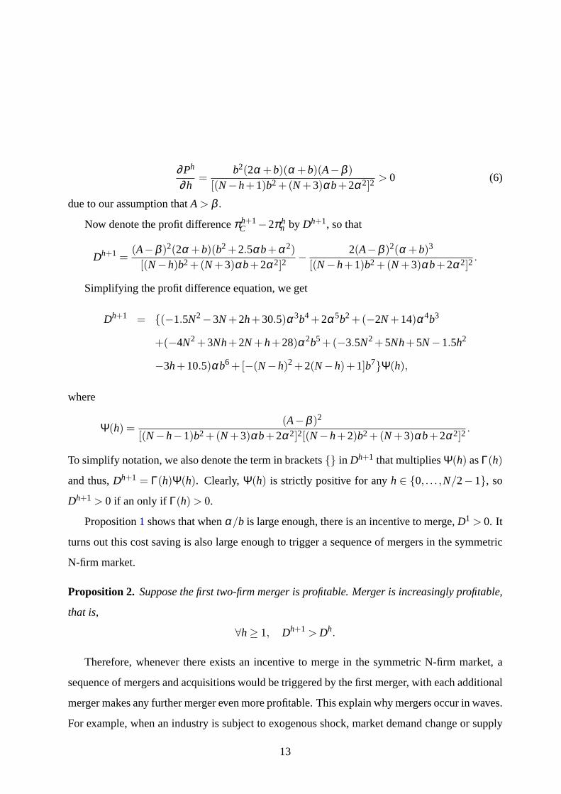
Simplifying the profit difference equation, we get

Dh+1 = {(−1.5N2−3N+2h+30.5)α3b4 +2α5b2 +(−2N+14)α4b3

+(−4N2 +3Nh+2N+h+28)α2b5 +(−3.5N2 +5Nh+5N−1.5h2

−3h+10.5)αb6 +[−(N−h)2 +2(N−h)+1]b7}Ψ(h),

where

Ψ(h) =(A−β )2

[(N−h−1)b2 +(N+3)αb+2α2]2[(N−h+2)b2 +(N+3)αb+2α2]2.

To simplify notation, we also denote the term in brackets{} in Dh+1 that multipliesΨ(h) asΓ(h)

and thus,Dh+1 = Γ(h)Ψ(h). Clearly,Ψ(h) is strictly positive for anyh ∈ {0, . . . ,N/2−1}, so

Dh+1 > 0 if an only if Γ(h) > 0.

Proposition1 shows that whenα/b is large enough, there is an incentive to merge,D1 > 0. It

turns out this cost saving is also large enough to trigger a sequence of mergers in the symmetric

N-firm market.

Proposition 2. Suppose the first two-firm merger is profitable. Merger is increasingly profitable,

that is,

∀h≥ 1, Dh+1 > Dh.

Therefore, whenever there exists an incentive to merge in the symmetric N-firm market, a

sequence of mergers and acquisitions would be triggered by the first merger, with each additional

merger makes any further merger even more profitable. This explain why mergers occur in waves.

For example, when an industry is subject to exogenous shock,market demand change or supply

13

shock that affects production costs, in our model,b decreases, orα increases, firms will have an

incentive to merge with each other. As each additional merger makes subsequent mergers more

profitable, we would expect a wave of merger activities in response to exogenous shocks that

changed firms’s cost, or market demand.

In addition, our model has another implication, that is, mergers may take place even if a two-

firm merger strictly reduce the total profit of merged firms. Tosee this, it is helpful to treat a wave

of mergers as a sequential-move game. Each additional merger makes previous mergers as well

as subsequent mergers more profitable. This is true as the reduced number of firms after mergers

will reduce competition in the market, pushing up market price and increasing firms’ profit.

We consider a market with N firms with each pair of firms separately making merger deci-

sions. Without loss of generality, assume N is an even number. As before, we focus on two-

firm mergers. In the sequential-move game of mergers, firms first make merger decisions and

then compete in output to realize their profits. Figure 1 shows the timing of events. We de-

note theM1,M2 . . . ,MN/2 as two-firms mergers in the sequence. Forj = 1,2, . . . ,N/2, let firms

(2M j − 1,2M j) be the two single-plant firms that can choose whether to “merge” or “not” to

merge into firmM j . Firms take turns to make choices, with firms 1,2 being the first to move and

firms N−1,N the last to move. Whenever two firms(2M j −1,2M j) play “not”, the game ends,

with M j−1 merged firms in the market while the rest of firms 2M j −1,2M j , . . . ,N remaining as

single plant firms. After the merging game ends, firms engage in Cournot competition to maxi-

mize profits. For example, if firm 1,2 choose not to merge, no merger would take place and the

game ends with no mergers and each firm would get a profit ofπ0(N). On the other hand, if all

pairs of firms, firms 1 and 2,. . ., and firmsN−1 andN choose “merge”, the game ends withN/2

mergers and each merged firm realizing a profit ofπN/2C .

We already know thatDh+1 = Γ(h)Ψ(h) andΨ(h) > 0 for all h, and will also show in the

appendix thatΓ(h) is strictly increasing inh. Thus, for some parameters(N,α,b), it may be the

case that mergerM j is not profitable,D j < 0, while mergerMk (k > j) is profitable given mergers

1, . . . ,Mk−1 have occurred. The extreme case of this scenario is thatDN/2 > 0 (or Γ(N/2−1) >

0), whileD j < 0 (orΓ( j −1) < 0) for j < N/2. The following result shows that even in this case,

14

Firm 1&2 merge

not

competitionπ0(N)/firm

3&4 merge

not

competition

realize profit

· · · · · · N-3&N-2 merge

not

competition

realize profit

N-1&N merge (πN/2C /firm)

not

competition

realize profit

Figure 1: Timing of events

merger wave may still take place.

Proposition 3. Suppose DN/2 > 0, all firms play “merge” in the unique subgame perfect Nash

equilibrium of the sequential-move game.

The conditionDN/2 > 0 implies that, conditional on all the other firms in the market have

merged, it is profitable for firmN−1 andN to play “merge.” However, the condition does not

state that the two-firm mergers between firm 1 and 2, between firm 3 and 4, etc., are profitable

by themselves. Suppose thatD1 < 0 but DN/2 > 0; the first two-firm merger is not profitable,

but the last merger would be profitable had all the previous pairs played “merge.” In this case,

we would expect a sequence of mergers to take place with everypair of firms (2M j − 1, 2M j )

choose “merge.” In fact, as long as the last two-firm merger isprofitable,DN/2 > 0, every pair of

firms playing “merge” is the unique subgame perfect Nash equilibrium of the sequential merger

game, even ifDh < 0 for all h < N/2. Hence, mergers and merger wave can take place even

if the mergers at the early stage of the wave are not profitableby themselves. This is true as

firms understand that, as the wave complete and competition is reduced, all merged firms will get

higher total profit than in the pre-merger market. This explains the puzzle that the announcement

period abnormal returns to acquirers are negative on average.

15

Schleifer and Vishny(2003) suggest that merger and acquisitions are driven by stock market

valuations. According to them, financial market is inefficient and thus, some firms may be valued

incorrectly. Managers of firms understand the market inefficiencies, and take advantage of them

through mergers and acquisitions. In their model, acquiring firm may be overvalued by the stock

market before the acquisition while the target firm may be undervalued. Another theory pro-

posed byGorton et al.(2005) suggest that mergers and merger waves can occur when managers

prefer to their firms to remain independent rather than acquired. They have assumed that large

firms are less likely to be acquired. Therefore, managers mayengage in unprofitable defensive

acquisitions, thereby reducing the chance of being acquired by another firm.

In contrast to the behavioral theories, none of the existingneoclassical theories can explain

the stylized fact of average negative announcement period returns. Therefore, the empirical ev-

idence seems to be in favor of the managerial incentive explanation. However, this need not be

so, as negative abnormal return does not have to contradict profit-maximization by firms, as the

current model shows. Our model predicts that there are casesin which the exogenous shock is

not sufficiently large to make early mergers profitable, but merger wave can still take place. This

means that some mergers, especially those at the early stageof the wave, may reduce the merged

firms’ total profit initially, while at the same time, profit for outside firms strictly increase. This

may result in a negative announcement period return for the acquiring firm, as an efficient stock

market reacts to the short-run unprofitable mergers. However, as the wave moves on, merged

firms’ profit gradually increase. Thus, our model also predicts that operation performance would

improve over time, whereas the behavior theories predict nosuch improvement in operating per-

formance post-merger.

This prediction of improved performance over time is consistent with the empirical findings

by some recent works on firms’ post-merger performance. One hypothesis of these studies is

that if mergers truly create value for shareholders, the gains would eventually show up in the

firms’ operating cash flows. Using samples from the U.S.,Healy, Palepu, and Ruback(1992)

and Switzer (1996) have reported statistically significant improvement in the post-acquisition

industry-adjusted operating cash flows.Linn and Switzer(2001) also find evidence of significant

16

improvements in industry-adjusted, operating cash flows post-takeover from a sample of U.S.

mergers. Using a sample of takeovers in the UK over the period1985–1993,Powell and Stark

(2005) report modest improvements in operating performance. Hence, the empirical evidence

suggest that mergers and acquisitions do increase firms’ performance and are profitable for firms

involved in the mergers.

3.3 Full-monopolization

For exposition purpose, we suppose that there are 2k (k∈ Z++) number of firms in the market

before any merger has happened,N = 2k. Also suppose there is an incentive to merge in the

symmetric pre-merger market,D1 > 0. Proposition2 indicates that the first merger triggers a

sequence of mergers, in which two firms form a two-plant firm. After the first wave of mergers,

the market is symmetric withN/2 larger firms, each of which now consists of 2 plants and has

the cost function

C(qC) =α2

q2C +βqC +θC.

What will happen in the post-merger market? Will there be any further incentives to merge? The

answer is yes. There is definitely an incentive for further mergers and acquisitions in the market.

Without any outside intervention, a second wave of mergers would ensue. Furthermore, new

waves of merger will take place after the second wave, well until the market is fully monopolized.

This result is summarized as follows.

Proposition 4. In a Cournot oligopoly market with N firms, where N= 2k, if a two-firm merger

is profitable, then N/2 round of mergers can take place until the market is fully monopolized.

Thus, if there ever exists an incentive to merge in a symmetric N-firm market, then, unless

blocked by the antitrust authority, the consolidation process could continue till there is only one

firm left in the market. Of course, this does not imply that full monopolization will take place in

real world, as antitrust authorities can block large mergers in concentrated market.

In the U.S., firms have been required to notify the antitrust authorities of all mergers above

a certain size since 1976. The antitrust enforcement agencymay require additional informa-

17

tion concerning the merger for further investigation. In some cases, the antitrust authority can

challenge the merger and prevent it from being completed. For example, recently, the Federal

Trade Commission has blocked Pepsi’s planned acquisition of7UP and Coca Cola’s acquisition

of Dr Pepper. In 2001, the U.S. Department of Justice blockedGeneral Dynamics’ merger with

Newport News Shipbuilding, the only other nuclear submarine builder for the U.S. Navy (Baker

2003). Therefore, there is probably little risk of monopolization with the existence of antitrust

policy. However, our analysis does show that one needs to take into account the benefits from

deterrence of antitrust law in quantifying the effect of antitrust policy on consumer welfare.

4 Merger and entry

In above we assume that entry is not possible and thus, any mergers necessarily reduces the

number of firms and with it competition in the market. This maybe appropriate for industries

in which there are barriers that make new entry too costly, but may not be realistic for many

industries in which entry barrier is not prohibitive. In what follows, we extend the basic model

by allowing entry by outside firms into the market under consideration.

To model firms’ entry and merger behavior, we assume that there are many but finite potential

entrepreneurs who might start a firm in this market. Entrepreneurs may have different abilities

operating a firm and this will have effect on firms total cost. We assume that the total costs of any

firm i in the market that is operatingmplants and producing outputqi are given by:

C(qi) =αq2

i

m+βqi +θi +Ei.

Each entrepreneur gets a draw ofEi from some distributionF with support[e,∞) wheree> 0. If

we think now about the original Cournot-Nash equilibrium with no mergers but entry, there will

be some number of firms, N, that are operating in the market, and these will be operated by the

N potential entrepreneurs who got the N lowest draws from thedistribution.

All firms in the no merger Cournot equilibrium will earn the samegross profitπi, where

πi =(A−β )2(b+α)

[b(N+1)+2α]2−θi.

18

But firms’ economic profitsΠi (net ofEi) will vary. Without loss of generality, we number the

firms 1,2, ....,N in order of increasingEi values, then firm N will be the marginal firm, in that it

is making just enough to keep its entrepreneur in this industry,

EN = π0(N).

Fact 1. No firm will exit the market after any mergers.

This is obvious as incumbent firms profits can not decrease in any merger equilibria. First,

the merged firm will not exit the market. For two firms to have anincentive to merge, their total

profit after the merger must be greater than before the mergerand thus, the merged firm should

not exit. Second, in the absence of entry, profit for each of the non-merged firms strictly increases

after any merger. This implies no incumbent will exit the market after any mergers.

A merger involves one entrepreneuri paying the other entrepreneurj to exit, with the merged

firm being operated by the remaining entrepreneuri. We assume that the entrepreneurj who sold

his firm can not enter the market again and thus, entry decision only involves entrepreneurs not

currently in the market. This assumption is made without loss of generality as in real world, any

buying-out contract always includes exclusive clause preventing the entrepreneur from entering

the same market in some period of time.

If the N-firm is marginal before the merger,

π0(N) = EN,

it turns out that allowing entry will have no effect on the incentive for the first merger.

Proposition 5. If firm N with EN has zero profit in the pre-merger equilibrium, then the incentive

for the first merger remains unchanged with or without entry.

Consider a N-firm market with (α,b) and entry barrier due to government regulations. Sup-

pose initially firm N breaks even and (α,b) is such thatα/b> ε2(N) and thus merger is profitable.

Now suppose the government deregulate and the entry barrieris removed, Proposition5 says that

merger remains profitable even when potential entrant mightenter the market. In fact, no entry

19

would occur after the first two-firm merger. The reason is simple. Prior to the merger, the N

firms are identical in technology, have same marginal cost atany given output. The firm with

the highest E breaks even. If a new firm enters the market afterthe first two-firm merger, the

post-merger post entry market would have N firms with one firm more efficient than the other

N-1 firms. This merged firm would produce more than the other N-1 firms. The profit for each

of the N-1 firm can not be greater than a firm’s profit before any merger and entry. This would

imply the firm with the highest E would have a loss in the post-merger post entry equilibrium.

Therefore, no entry would occur even if in post-merger market, all firms make positive profits.

Proposition 1 still holds, even if entry is allowed.

Of course, this result relies upon the assumption that in thepre-merger equilibrium, firm N

is marginal. This may not be true if we allowed the possibility that in the original no-merger

equilibrium,

π0(N) > EN but π0(N+1) < EN+1.

In this case, a two-firm merger may induce subsequent entry byfirm N+1 into the market. How-

ever, the first merger does not induce entry only ifEN+1 is large, for example, if

EN+1 ≥ π0(N),

that is, firm N+1 could not profitably enter the pre-merger market when there were only N-1

firms.

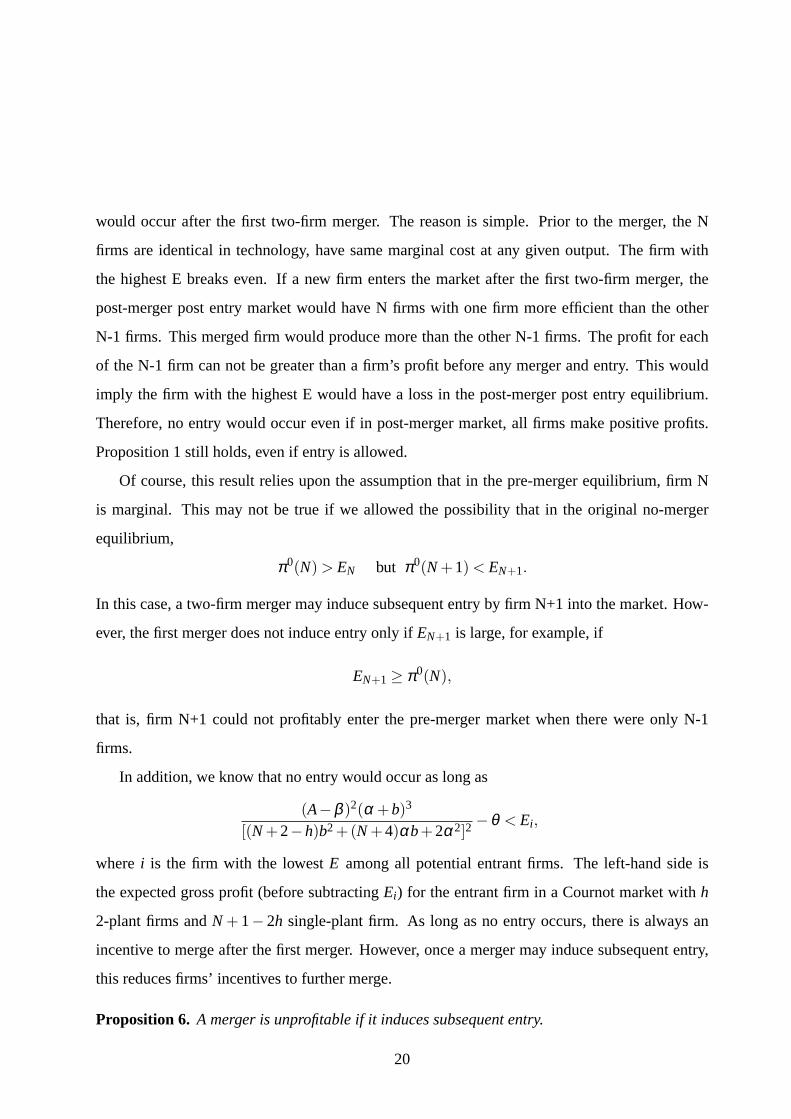
In addition, we know that no entry would occur as long as

(A−β )2(α +b)3

[(N+2−h)b2 +(N+4)αb+2α2]2−θ < Ei,

where i is the firm with the lowestE among all potential entrant firms. The left-hand side is

the expected gross profit (before subtractingEi) for the entrant firm in a Cournot market withh

2-plant firms andN + 1−2h single-plant firm. As long as no entry occurs, there is alwaysan

incentive to merge after the first merger. However, once a merger may induce subsequent entry,

this reduces firms’ incentives to further merge.

Proposition 6. A merger is unprofitable if it induces subsequent entry.

20

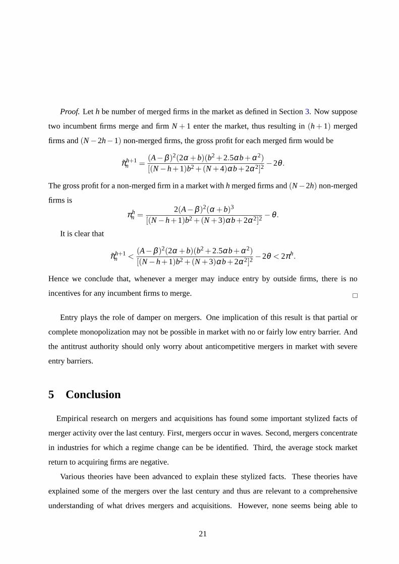
Proof. Let h be number of merged firms in the market as defined in Section3. Now suppose

two incumbent firms merge and firmN + 1 enter the market, thus resulting in(h+ 1) merged

firms and(N−2h−1) non-merged firms, the gross profit for each merged firm would be

πh+1n =

(A−β )2(2α +b)(b2 +2.5αb+α2)

[(N−h+1)b2 +(N+4)αb+2α2]2−2θ .

The gross profit for a non-merged firm in a market withh merged firms and(N−2h) non-merged

firms is

πhn =

2(A−β )2(α +b)3

[(N−h+1)b2 +(N+3)αb+2α2]2−θ .

It is clear that

πh+1n <

(A−β )2(2α +b)(b2 +2.5αb+α2)

[(N−h+1)b2 +(N+3)αb+2α2]2−2θ < 2πh.

Hence we conclude that, whenever a merger may induce entry byoutside firms, there is no

incentives for any incumbent firms to merge.

Entry plays the role of damper on mergers. One implication ofthis result is that partial or

complete monopolization may not be possible in market with no or fairly low entry barrier. And

the antitrust authority should only worry about anticompetitive mergers in market with severe

entry barriers.

5 Conclusion

Empirical research on mergers and acquisitions has found some important stylized facts of

merger activity over the last century. First, mergers occurin waves. Second, mergers concentrate

in industries for which a regime change can be be identified. Third, the average stock market

return to acquiring firms are negative.

Various theories have been advanced to explain these stylized facts. These theories have

explained some of the mergers over the last century and thus are relevant to a comprehensive

understanding of what drives mergers and acquisitions. However, none seems being able to

21

reconcile all stylized facts. Therefore, there is room for an alternative model as we present in this

paper.

We consider a model of horizontal mergers between Cournot firms that have quadratic costs.

While retaining the assumptions of profit-maximizing firms and efficient stock market, it can still

accommodate all three stylized facts. According to our model, both high cost-savings from a

merger or a small slope for inverse market demand increase the incentive to merge. In addition,

the profitability of any merger increases with the number of mergers having already taken place.

One implication following the increasing profitability prediction is that mergers tend to occur in

waves. Another implication is that some mergers not profitable for the merged firms in the short-

run may take place at the early stage of a wave, which explainsthe findings of negative average

return without violating the profit-maximization paradigm.

Appendix

Proof of Proposition 1.

First, note that the profit differenceD(2) can be written as

(A−β )2[(−1.5N2 +N+8.5)αb4 +(10−2N)α2b3 +2α3b2 +(−N2 +2N+1)b5]

[Nb2 +Nαb+3αb+2α2]2[b(N+1)+2α]2(A.1)

The sign ofD(2) is determined by its numerator, and this is strictly positive if and only if

(−1.5N2 +N+8.5)αb4 +(10−2N)α2b3 +2α3b2 +(−N2 +2N+1)b5 > 0, (A.2)

which can be re-written as:

2α3b2 > K(N)αb4 +L(N)α2b3 +M(N)b5

with K(N) = 1.5N2−N+8.5, L(N) = 2N−10 andM(N) = N2−2N−1. Note that all three of

these functions are increasing inN for N ≥ 2. Now, divide this expression byα2b3 to get:

2αb

> K(N)bα

+L(N)+M(N)(bα

)2

22

Now, note that the LHS is increasing inε ≡ α/b, while the RHS is decreasing inε. Thus, for any

value ofN, it is possible to find a value ofε large enough that the inequality holds.

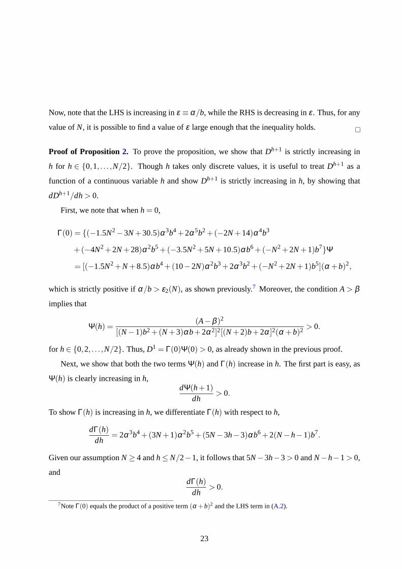
Proof of Proposition 2. To prove the proposition, we show thatDh+1 is strictly increasing in

h for h ∈ {0,1, . . . ,N/2}. Thoughh takes only discrete values, it is useful to treatDh+1 as a

function of a continuous variableh and showDh+1 is strictly increasing inh, by showing that

dDh+1/dh> 0.

First, we note that whenh = 0,

Γ(0) = {(−1.5N2−3N+30.5)α3b4 +2α5b2 +(−2N+14)α4b3

+(−4N2 +2N+28)α2b5 +(−3.5N2 +5N+10.5)αb6 +(−N2 +2N+1)b7}Ψ

= [(−1.5N2 +N+8.5)αb4 +(10−2N)α2b3 +2α3b2 +(−N2 +2N+1)b5](α +b)2,

which is strictly positive ifα/b > ε2(N), as shown previously.7 Moreover, the conditionA > β

implies that

Ψ(h) =(A−β )2

[(N−1)b2 +(N+3)αb+2α2]2[(N+2)b+2α]2(α +b)2 > 0.

for h∈ {0,2, . . . ,N/2}. Thus,D1 = Γ(0)Ψ(0) > 0, as already shown in the previous proof.

Next, we show that both the two termsΨ(h) andΓ(h) increase inh. The first part is easy, as

Ψ(h) is clearly increasing inh,dΨ(h+1)

dh> 0.

To showΓ(h) is increasing inh, we differentiateΓ(h) with respect toh,

dΓ(h)

dh= 2α3b4 +(3N+1)α2b5 +(5N−3h−3)αb6 +2(N−h−1)b7.

Given our assumptionN ≥ 4 andh≤ N/2−1, it follows that 5N−3h−3> 0 andN−h−1> 0,

anddΓ(h)

dh> 0.

7NoteΓ(0) equals the product of a positive term(α +b)2 and the LHS term in (A.2).

23

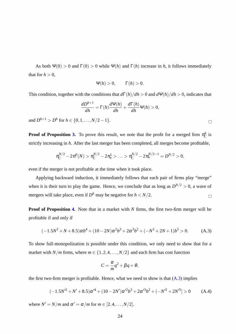
As bothΨ(0) > 0 andΓ(0) > 0 while Ψ(h) andΓ(h) increase inh, it follows immediately

that forh > 0,

Ψ(h) > 0, Γ(h) > 0.

This condition, together with the conditions thatdΓ(h)/dh> 0 anddΨ(h)/dh> 0, indicates that

dDh+1

dh= Γ(h)

dΨ(h)

dh+

dΓ(h)

dhΨ(h) > 0,

andDh+1 > Dh for h∈ {0,1, . . . ,N/2−1}.

Proof of Proposition 3. To prove this result, we note that the profit for a merged firmπhC is

strictly increasing inh. After the last merger has been completed, all merges becomeprofitable,

πN/2C −2π0(N) > πN/2

C −2π1n > .. . > πN/2

C −2πN/2−1n = DN/2 > 0,

even if the merger is not profitable at the time when it took place.

Applying backward induction, it immediately follows that each pair of firms play “merge”

when it is their turn to play the game. Hence, we conclude thatas long asDN/2 > 0, a wave of

mergers will take place, even ifDh may be negative forh < N/2.

Proof of Proposition 4. Note that in a market withN firms, the first two-firm merger will be

profitable if and only if

(−1.5N2 +N+8.5)αb4 +(10−2N)α2b3 +2α3b2 +(−N2 +2N+1)b5 > 0. (A.3)

To show full-monopolization is possible under this condition, we only need to show that for a

market withN/mfirms, wherem∈ {1,2,4, . . . ,N/2} and each firm has cost function

C =αm

q2 +βq+θ ,

the first two-firm merger is profitable. Hence, what we need to show is that (A.3) implies

(−1.5N′2 +N′ +8.5)α ′4 +(10−2N′)α ′2b3 +2α ′3b2 +(−N′2 +2N′5] > 0 (A.4)

whereN′ = N/mandα ′ = α/m for m∈ [2,4, . . . ,N/2].

24

Whenm= 2, the condition in (A.4) becomes

18

[

(−1.5N2 +2N+34)αb4 +(20−2N)α2b3 +2α3b2 +(−2N2 +8N+8)b5]]

=18

[

(−1.5N2 +N+8.5)αb4 +(10−2N)α2b3 +2α3b2 +(−N2 +2N+1)b5+

+ (N+25.5)αb4 +10α2b3 +(−N2 +6N+7)b5]

For the discussion to be meaningful, there should be at least4 firms in the market,N ≥ 4. In

this case,

(−1.5N2 +2N+8.5) < (−N2 +2N+1) < 0, (10−2N) ≤ 2.

Clearly, (A.3) implies thatα > b. WhenN = 4, (−N2 + 6N + 7) > 0 and thus, (A.3) implies

(A.4). WhenN > 4, (A.3) would also implies that

2α3b+(−1.5N2 +N+8.5)αb4 > 0.

But

(N+25.5)αb4 +10α2b3 +(−N2 +6N+7)b5

> (N+25.5)αb4 +8α2b3 +bα

[2α3b2 +(−1.5N2 +N+8.5)αb4]

> 0

Consequently, whenN > 4, (A.3) implies that (A.4) holds. Thus we can conclude that if the first

two-firm merger is profitable in market withN firms, the subsequent two-firm merger between

merged firm withm≥ 2 plants is also profitable.

Proof of Proposition5. When firm N is marginal, it breaks even in the pre-merger Cournot

equilibrium,

EN = π0(N) =(A−β )2(b+α)

[b(N+1)+2α]2+2θi −θi.

Now suppose firm N+1 enters the market, gross profit for each ofthe non-merged firm would be

π1(N) =(A−β )2(b+α)3

[(N+1)b2 +(N+4)αb+2α2]2−θi < Π0(N).

This implies thatEN+1 > π1(N) and firm N+1 suffers a loss by entering the market.

25

References

Andrade, G., M. Mitchell, and E. Stafford (2001). New evidence and perspectives on mergers.

Journal of Economic Perspectives 15, 103–20.

Andrade, G. and E. Stafford (2004). Investigating the economic role of mergers.Journal of

Corporate Finance 10, 1–36.

Baker, J. B. (2003). The case for antitrust enforcement.Journal of Economic Perspective 17,

27–50.

Banal-Estanol, A. (2005). Information-sharing implications of horizontal mergers. working

paper.

Banerjee, A. and J. Owers (1992). Wealth reduction in white knight bids. Financial Manage-

ment 21, 48–57.

Bradley, M., A. Desai, and H. Kim (1988). Synergistic gains from corporate acquisition and

their division between stockholders of target and acquiring firms. Journal of Financial Eco-

nomics 21, 3–40.

Byrd, J. and K. Kickman (1992). Do outside directors monitor managers.Journal of Financial

Economics 32(2), 195–221.

Crandall, R. W. and C. Winston (2003). Does antitrust policy improve consumer welfare? As-

sessing the evidence.Journal of Economic Perspective 17(4), 3–26.

Deneckere, R. and C. Davidson (1985). Incentives to form coalition with Bertrand competition.

Rand Journal of Economics 16.

Gorton, G., M. Kahl, and R. Rosen (2005). Eat or be eaten: a theory of mergers and merger

waves. working paper, the Wharton School.

Harford, J. (2005). What drives merger waves?Journal of Financial Economics 77(3), 529–60.

26

Healy, P., K. Palepu, and R. Ruback (1992). Does corporate performance improve after mergers?

Journal of Financial Economics 31, 135–75.

Heywood, J. S. and M. McGinty (2007). Convex costs and the merger paradox revisited.Eco-

nomic Inquiry 45, 342–349.

Jennings, R. and M. Mazzeo (1991). Stock price movements around acquisition announcements

and management’s response.Journal of Business 64(2), 139–63.

Kamien, M. I. and I. Zang (1990). The limits of monopolization through acquisition.Quarterly

Journal of Economics 5, 323–338.

Kamien, M. I. and I. Zang (1991). Competitively cost advantageous mergers and monopolization.

Games and Economic Behavior 5, 323–338.

Linn, S. and J. Switzer (2001). Are cash acquisitions associated with better better post combi-

nation operating performance than stock acquisitions?Journal of Banking and Finance 25,

1113–38.

Mitchell, M. and J. H. Mulherin (1996). The impacts of industry shocks on takeover and restruc-

turing activity. Journal of Financial Economics 41, 193–229.

Morck, R., A. Schleifer, and R. Vishny (1990). Do managerial incentives drives bad acquisitions.

Journal of Finance 45, 31–48.

Perry, M. K. and R. H. Porter (1985). Oligopoly and the incentive for horizontal merger.Ameri-

can Economic Review 75, 219–27.

Powell, R. G. and A. W. Stark (2005). Does operating performance increase post-takeover for

uk takeovers? A comparison of performance measures and benchmarks.Journal of Corporate

Finance 11, 293–317.

Rhodes-Kropf, M. and S. Viswanathan (2004). Market valuation and mergers.Journal of Fi-

nance 59(6), 2685–2718.

27

Salant, S., S. Switzer, and R. Reynolds (1983). Losses due to merger: the effects of an exogenous

change in industry structure on Cournot-Nash equilibrium.Quarterly Journal of Economics 98.

Schleifer, A. and R. Vishny (2003). Stock market driven acquisitions. Journal of Financial

Economics 70, 295–311.

Stigler, G. J. (1950). Monopoly and oligopoly by merger.American Economics Review Proceed-

ings 40, 23–34.

Switzer, J. (1996). Evidence of real gains in corporate acquisitions. Journal of Economics and

Business 48, 443–460.

28