Mixing of non-Newtonian fluids in time-periodic cavity flows

J. Non-Newtonian Fluid Mech. 93 (2000) 265–286

Mixing of non-Newtonian fluids in time-periodic cavity flows

Patrick D. Anderson∗, Oleksiy S. Galaktionov, Gerrit W.M. Peters, Frans N. van de Vosse,Han E.H. Meijer

Materials Technology, Dutch Polymer Institute, Eindhoven University of Technology,P.O. Box 513, WH 0.117, 5600 MB Eindhoven, The Netherlands

Received 25 October 1999; received in revised form 7 March 2000

Abstract

Fluid mixing in two- and three-dimensional time-periodic cavity flows as a function of rheological fluid param-eters is studied. Computational methods are applied to obtain accurate descriptions of the velocity fields, whichform the basis of the mixing analysis. In addition to some classical techniques, like Poincaré maps and the analysisof periodic points, a recently developed mapping method is used to determine mixing efficiency over a wide rangeof different flow parameters. Within this framework, different mixing protocols can be evaluated with respect totheir long term mixing behaviour and compared quantitatively. It is shown that local ‘optimal’ parameter settingsfor mixing of Newtonian fluids can result in a considerable worse mixing behaviour for non-Newtonian fluids, andvice versa, illustrating the importance of taking the rheology of the fluid into account. © 2000 Elsevier Science B.V.All rights reserved.

Keywords:Mixing; Chaotic advection; Cavity flow

1. Introduction

Many fluids in nature and industrial processes show a non-Newtonian fluid behaviour. The viscositycan depend on the shear-rate, or the stresses can depend on the history of the deformation, or both. Despitethe fact that the importance of non-Newtonian fluids in industrial processes is recognised in a wide rangeof studies, only a few studies have been published on mixing of non-Newtonian fluids. Early venturesto describe and understand mixing processes are by Spencer and Wiley [28], Danckwerts [9], and Biggand Middleman [6]. Recently, mixing of viscous liquids has been associated with the chaotic behaviourof a dynamical system. Aref [4] studied thechaotic advectionof passive tracers by the flow of twoalternatively rotating point vortices, called theblinking vortex flow. During mixing in such deterministicchaotic flows, complex structures of folds are observed which could be well-defined by considering the

∗ Corresponding author. Tel.:+31-4024-79111; fax:+31-4024-47355.E-mail address:[email protected] (P.D. Anderson)

0377-0257/00/$ – see front matter © 2000 Elsevier Science B.V. All rights reserved.PII: S0377-0257(00)00120-8

266 P.D. Anderson et al. / J. Non-Newtonian Fluid Mech. 93 (2000) 265–286

flow as a Hamiltonian dynamical system. Soon these ideas were adopted for other types of flow, as forexample thejournal bearing flow[7], and thelid-driven cavity flow[8].

The studies involving non-Newtonian fluids are roughly divided into two parts; one concerning purelyelastic non-Newtonian fluids, the other dealing with inelastic non-Newtonian fluid behaviour. Niederkornand Ottino [22] reported on chaotic advection in the journal bearing flow for shear-thinning, fluids, andLing and Zhang [18] examined the influence of the deformation-rate-dependent viscosity onmixingwindows— regions in the parameter space where mixing systems are nearly chaotic. These studiesdescribe a decrease in the quality of mixing for the inelastic fluids compared to Newtonian fluids, bothin rate and in extent. Noteworthy is that already significant effects are observed with less than 5%difference in the velocity field (in theL∞ norm) compared to the Newtonian results. It was observed thatshear-thinning reduces the strength of vortices and weakens the link between high and low shear-rateregions. Hence, the mixing performance degrades.

For a particular class of viscoelastic fluids some results have been presented in the literature. If therelaxation time of the fluid is small compared to the characteristic time of the period of a time-periodicflow, the Deborah number is small and quasi-stationary flow can be assumed. Leong and Ottino [16]experimentally studied the effect of addition of polymer to a Newtonian fluid undergoing chaotic advec-tions in a two-dimensional time-periodic cavity flow. Two different mixing protocols were applied, oneflow that is discontinuous in time consisting of an alternating moving top and bottom wall, the other acontinuous (sinusoidal) wall movement. In both cases they observed large effects of the Deborah numberon the mixing behaviour at relatively low Deborah numbers (defined as the ratio of fluid relaxation timeand duration of a flow period) in the order of 0.5. Niederkorn and Ottino [21] presented experiments andsimulations in the journal bearing flow involving planar creeping flow between eccentric cylinders. Eachcylinder boundary has an angular velocity that behaves like a square wave as a function of time, creatingrectangular pulses, and thus the flow possesses a characteristic period. Their experiments show that thearea of the flow domain containing chaotic fluid particle trajectories can either increase or decrease,compared to the Newtonian case, depending on the periods associated with the boundary motion. Theseeffects occur for a Weissenberg number (defined as the product of a fluid relaxation time and a charac-teristic shear rate) as low as 0.04. Another more recent study on chaotic advection in creeping flow ofviscoelastic fluids in the journal bearing flow is by Kumar and Homsy [15]. They used perturbation theoryfor low levels of elasticity to determine semi-analytically the viscoelastic correction to the Newtonianflow field, based on the Oldroyd-B constitutive model. Their goal was to predict how elasticity affectschaotic advection in quasi-steady flows. It was found that elasticity can act to either increase or decreasethe area over which chaotic advection occurs, depending on the boundary motion.

For more realistic viscoelastic mixing flows, the analyses are more complicated because of the memoryof the fluids. In general, for viscoelastic flows, the transition of the flow between time intervals can not beneglected when external excitations are changed. Generally, viscoelastic computations in complex flowsat high Weissenberg numbers has proven to be a tremendous challenge, in particular for systems wheresingularities are present. Examples include cavity flows with a steadily moving lid, and only a limitednumber of computational methods provide satisfactory results [5]. The development of stable algorithmswhich can handle time-dependent problems (with or without singularities) is even a harder task; seefor example, the work of Grillet et al. [11] who studied elastic effects in cavity flows. Another issue ofimportance in viscoelastic flow computations is the choice of a proper constitutive model, which describesthe fluid well both under shear and elongation. Although a variety of constitutive models are available,the choice of the model and the choice of the linear and non-linear fluid parameters is a difficult task

P.D. Anderson et al. / J. Non-Newtonian Fluid Mech. 93 (2000) 265–286 267

[24,26]. Due to these difficulties associated with viscoelastic flow modelling, this paper only considersfluids with an inelastic non-Newtonian rheological fluid behaviour, and future work will cope with theventure of viscoelastic mixing flows at high Weissenberg numbers.

The paper discusses the influences of a shear-rate-dependent viscosity on mixing in two- and three-dimensional prototypical mixing flows, and the Carreau model is used. Results presented here can beused in the future as a reference for viscoelastic mixing flows exhibiting shear-thinning. The goal of thepaper is two-fold. First, details of mixing are studied using Poincaré maps, periodic points, and advectionof fluid elements. Second, optimisation of the mixing protocol is investigated using a ‘mapping’ method.In all cases, the influence of rheological parameters (the power-law index and the Carreau number) onthe mixing process is studied.

2. Mathematical formulation and numerical techniques

The rheological model used throughout this paper is the Carreau model with zero infinite-shear-rateviscosity

η = η0(1 + (λγ )2

)(n−1)/2, (1)

wheren is the power-law parameter,λ the time constant andη0 is the zero shear-rate viscosity. Thismodel has advantages over the more simple power-law model, since most fluids exhibit a low shear-rateNewtonian plateau and a transition region into the power law regime. The Carreau model accounts forboth aspects. The shear-rateγ used in Eq. (1) is defined asγ = √

II2DDD, whereIIDDD = (1/2)(Tr2(DDD) −Tr(DDD2)) is the second invariant of the rate of deformation tensorDDD = (1/2)(∇uuu+ (∇uuu)c). The followingdimensionless numbers characterise the shear-thinning nature of the flow:• the shear-thinning index or power-law parametern,• the Carreau number, Cr= λU/L, which can be regarded as a dimensionless shear-rate.The dimensionless form of the conservation equations read

St∂uuu

∂t+ uuu · ∇uuu = −∇p + 1

Re∇ · 2η∗DDD, η∗ = η

η0, ∇ · uuu = 0. (2)

The Reynolds number, Re= ρUL/η0, is defined here using the zero shear-rate viscosityη0, and St=L/UT is the Strouhal number.L is the characteristic length,U the characteristic velocity,T the charac-teristic time, andρ is the density of the fluid.

The time-periodic flows considered are such that Re and St are small and, as a result, the transientbehaviour of the velocity field during switching of cavity wall motions can be neglected, see Fig. 1.The flows are, therefore, approximated as piece-wise steady, and to obtain a solution of Eq. (2) withappropriate boundary conditions, the quasi-stationary Stokes equations are solved to obtain the velocityfield. Since no analytical solutions are available for the generalised Newtonian Stokes flow in a lid-drivencavity, numerical techniques are required, like boundary integral methods, finite difference, or finiteelement methods. As small changes in the velocity field will give rise to different advection patterns, thenumerical integration of chaotic particle trajectories requires an accurate approximation of the velocityfield. For this reason a spectral element method [19] has been used. The main advantage of a high-orderspectral method is that, in comparison with classical low-order finite element, finite volume, and finitedifference methods, far less degrees of freedom are required to achieve a desired level of high accuracy.


The time discretisation is based on an approximate pressure correction scheme for Newtonian fluids [29],and was extended for shear-rate dependent fluids [1]. It essentially reformulates the original problem intoa Helmholtz equation for the velocity, and a Poisson equation for a pressure-related quantity.

3. Mixing in two-dimensional cavity flows

The key to effective mixing lies in producing repetitive stretching and folding, an operation referred to asa horseshoe map in the mathematics literature. The existence of horseshoe maps indicates that the systemis chaotic (see [23] for definitions of chaos in dynamical systems). If we consider a two-dimensionalsteady velocity field, then the velocity field is integrable and the mixing cannot be chaotic [12,23]. Fluidtravels over closed streamlines and the mixing is thus poor: stretching is linear and no folds are created.On the other hand, if the velocity field is time-dependent, for example time-periodic, there is a goodchance that the system is chaotic; particles initially close are spread through the whole flow domain. Anecessary condition for chaos is the crossing of streamlines. A well-known example of a two-dimensionalchaotic flow is a time-periodic cavity flow generated by alternately moving the upper and lower wall fora fixed time period.

The objective here is to analyse the influence of shear-thinning on mixing in a two-dimensional cavitywith a time-periodic motion using the so-called TB protocol, see Fig. 1, thus applying a consecutivemovement of the top (front) and bottom (back) walls. This flow configuration is extensively studied, bothexperimentally and theoretically, in the literature for Newtonian fluids, see for example [2,17,23], is usedas a prototype flow. In Section 4 a three-dimensional extension of the two-dimensional cavity flow isconsidered, see Fig. 1. Since a quasi-static steady velocity field is assumed, only one single velocity fieldcomputation for the motion of a single wall is required, and the other field, as a result of a constant motionof the opposite wall, is simply found by a coordinate transformation.

The aspect ratio of the two-dimensional cavity is chosen to be the same as in previous studies byLeong and Ottino [17] and others, and equals 5:3. The flow domain�, depicted in Fig. 1, ish < x <

h, (h = 5/3) − 1 < y < 1, is subdivided into 15× 9 spectral elements of 12th order, the mesh being

Fig. 1. Schemes of the two- and three-dimensional cavity, In both protocols during the first half of the period the top (back)wall is moved from left to right, and in the second half of the period the opposite (front) wall is moved from right to left. Thisprotocol is denoted as the TB protocol.


refined near the moving top wall. The Newtonian velocity field is computed and taken as an initialcondition, and the time integration of the pressure correction scheme is continued until a steady statefor the non-Newtonian fluid is reached. The criterion used to terminate the integration is based on therelative differenceε = ‖uuui+1 − uuui‖∞/‖uuui+1‖∞, whereuuui denotes the velocity field afteri iterations,and‖ . . . ‖∞ denotes the maximum norm. The toleranceε to terminate the integration was set equal to10−6.

Mixing in this cavity is studied forn = 0.2, 0.4, 0.6, 0.8, and 1.0 in Eq. (1), leading to four shear-thin-ning fluids and the Newtonian fluid (n = 1), which spans the range of shear-thinning behaviour forpractical fluids. In the remainder of this section the Carreau number, Cr, is fixed at Cr= 5, meaning thatshear-thinning behaviour is clearly present in the flow, and the fluid behaves like a power-law fluid. First,the influence of the shear-rate-dependent viscosity on the velocity field is studied. Second, the impacton mixing is analysed using Poincaré maps, chaotic advection of fluid elements, and determination anddiagnosing first-order periodic points. Finally, the mapping method is used to study mixing for a widerange of dimensionless wall displacements.

3.1. Velocity field

Fig. 2 shows the velocity profiles (Re= 0) along two lines in the cavity, when the top wall has aconstant dimensionless velocityu = 1. The lines on the left show the result for thex component of thevelocity atx = −1.5; the other lines are results for the velocity at the centre linex = 0. Only smalldeviations from the Newtonian velocity field are detectable near the stationary side walls of the cavity, butin the centre of the cavity the differences are more significant and increase asn decreases: shear-thinningreduces the influence of the moving top wall in the core of the cavity. A typical viscosity distributionin the cavity for the Carreau fluid with parametersn = 0.6 and Cr= 5 is given in Fig. 3, showing thesymmetry of the viscosity and the range of viscosities spanned.

3.2. Poincaré maps

The Poincaré map is one of the most simple methods to analyse chaotic mixing flows and is a powerfulway to reveal zones of regular and chaotic motion. Once the velocity field has been computed, the analysis

Fig. 2. Thex component of the velocity along the linesx = −1.5 andx = 0.


Fig. 3. The normalised viscosity distribution in a cavity with a moving top wall for a Carreau fluid with parametersn = 0.6 andCr = 5. The viscosity is symmetrical with respect to the vertical centre line.

of the chaotic dynamics is based on integration of material points coordinates

dxxx

dt= uuu(xxx, t), (3)

and the time dependence ofuuu is the source of any chaotic behaviour in the system. The integration ofEq. (3) with the initial conditionxxx = X0X0X0 at t = 0 for a time lengthT gives the position of particlexxx att = T . The flow can be represented by the motion

xxx = 888t(XXX), XXX = 888t=0(XXX), (4)

mapping particleXXX to the positionxxx after a timet . The Poincaré section allows a systematic reduction incomplexity of problems by reduction of the number of dimensions [12]. Successive intersections of orbitsof a pointxxx1 after a timet = T define a mapxxxn+1 = 8(xxxn). The pointxxx1 is mapped toxxx2 = 8(xxx1),the pointxxx2 is mapped toxxx3 = 8(xxx2) = 82(xxx1), and so on. The Poincaré map is constructed byplotting all intersections. Note that this viewpoint is purely kinematic and all the complexities in solvingthe dynamical system are associated with obtaininguuu(xxx, t). The dynamical system (3) is numericallyintegrated using an adaptive Runge–Kutta scheme, see [25], and errors in the trajectories of particles aremainly imposed by discretisation errors of the numerical velocity field [27]. It should be noted that theparticles are passive markers within the fluid, i.e. there is no diffusion of particles.

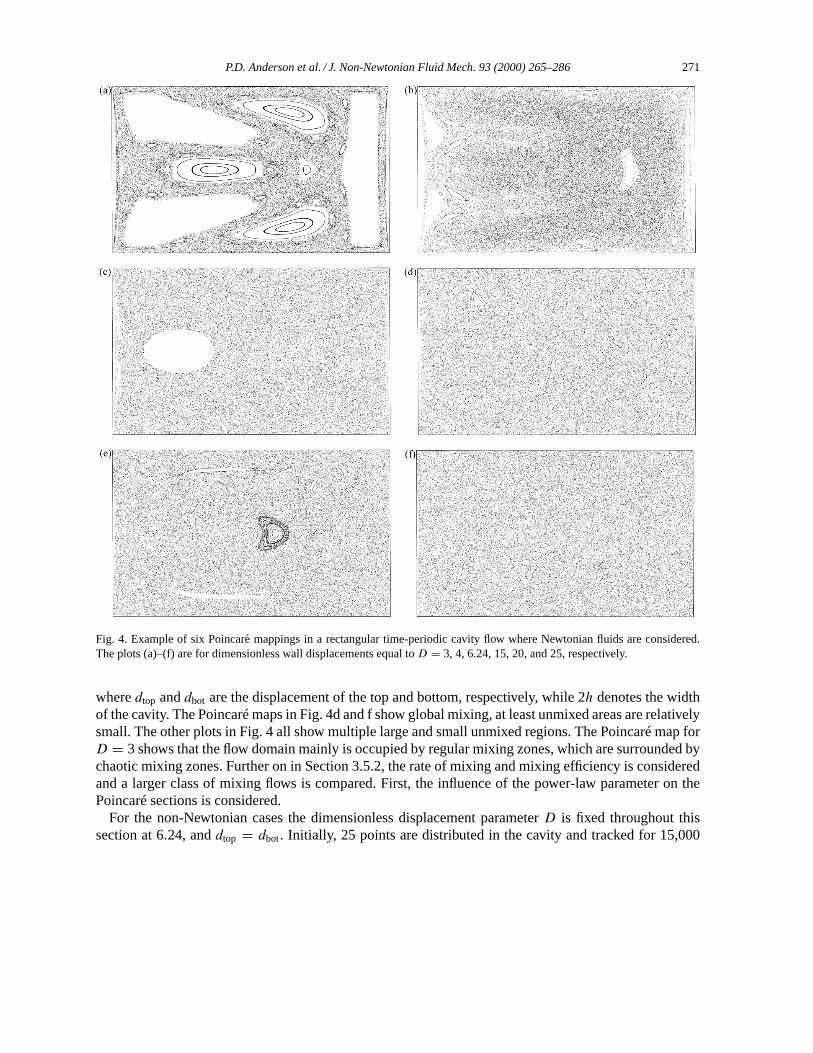
In Fig. 4 six examples of Poincaré sections for a Newtonian fluid in a time-periodic cavity flow, inducedby consecutive motion of top and bottom wall, are presented for a dimensionless wall displacementD = 3,4, 6.24, 15, 20, and 25, defined as

D = ‖dtop‖ + ‖dbot‖2h

, (5)


Fig. 4. Example of six Poincare mappings in a rectangular time-periodic cavity flow where Newtonian fluids are considered.The plots (a)–(f) are for dimensionless wall displacements equal toD = 3, 4, 6.24, 15, 20, and 25, respectively.

wheredtop anddbot are the displacement of the top and bottom, respectively, while 2h denotes the widthof the cavity. The Poincaré maps in Fig. 4d and f show global mixing, at least unmixed areas are relativelysmall. The other plots in Fig. 4 all show multiple large and small unmixed regions. The Poincaré map forD = 3 shows that the flow domain mainly is occupied by regular mixing zones, which are surrounded bychaotic mixing zones. Further on in Section 3.5.2, the rate of mixing and mixing efficiency is consideredand a larger class of mixing flows is compared. First, the influence of the power-law parameter on thePoincaré sections is considered.

For the non-Newtonian cases the dimensionless displacement parameterD is fixed throughout thissection at 6.24, anddtop = dbot. Initially, 25 points are distributed in the cavity and tracked for 15,000


Fig. 5. Poincare maps for Carreau fluids with (a)n = 0.8, (b) 0.6, (c) 0.4, and (d) 0.2, where the flow consists of a consecutivemotions of the top and bottom walls. The dimensionless wall displacementD equals 6.24. Compare with the Newtonian casen = 1 in Fig. 4c.

periods. The positions of these points after each period are plotted in the figure. These (asymptotic)pictures show that for increasingD the regions of chaotic and regular mixing change. A comparisonof the Poincaré map for the Newtonian fluid, presented in Fig. 4c, and the Carreau fluid, presented inFig. 5 withn = 0.8, shows that the main island is still present, but its size has decreased. For two lowervalues of the power law parametern, i.e. n = 0.6 and 0.4, the asymptotic pictures show more globalmixing. Forn = 0.2 a large number of islands, mainly around high-order elliptic periodic points (seealso forthcoming sections), is observed. These resultsappearto show that the mixing is improved forstronger shear-thinning fluids whenD = 6.24. However, while the parametersn = 0.6 and 0.4 display amore uniform asymptotic mixture, it will be shown that the rate of mixing is considerably lower than foreither the Newtonian fluid or the Carreau fluid withn = 0.8. More details of the chaotic behaviour of theflow are revealed by analysing the chaotic advection of fluid elements and studying the periodic points.This is the subject of the following paragraphs.

3.3. Chaotic advection

Further indication of the rate of mixing can be obtained by examining the advection of a fluid strip inthe cavity. Tracking of strongly deforming fluid elements is efficiently performed by application of anadaptive front tracking technique [10,31]. An initial strip, shown in Fig. 6, is tracked for two periods for


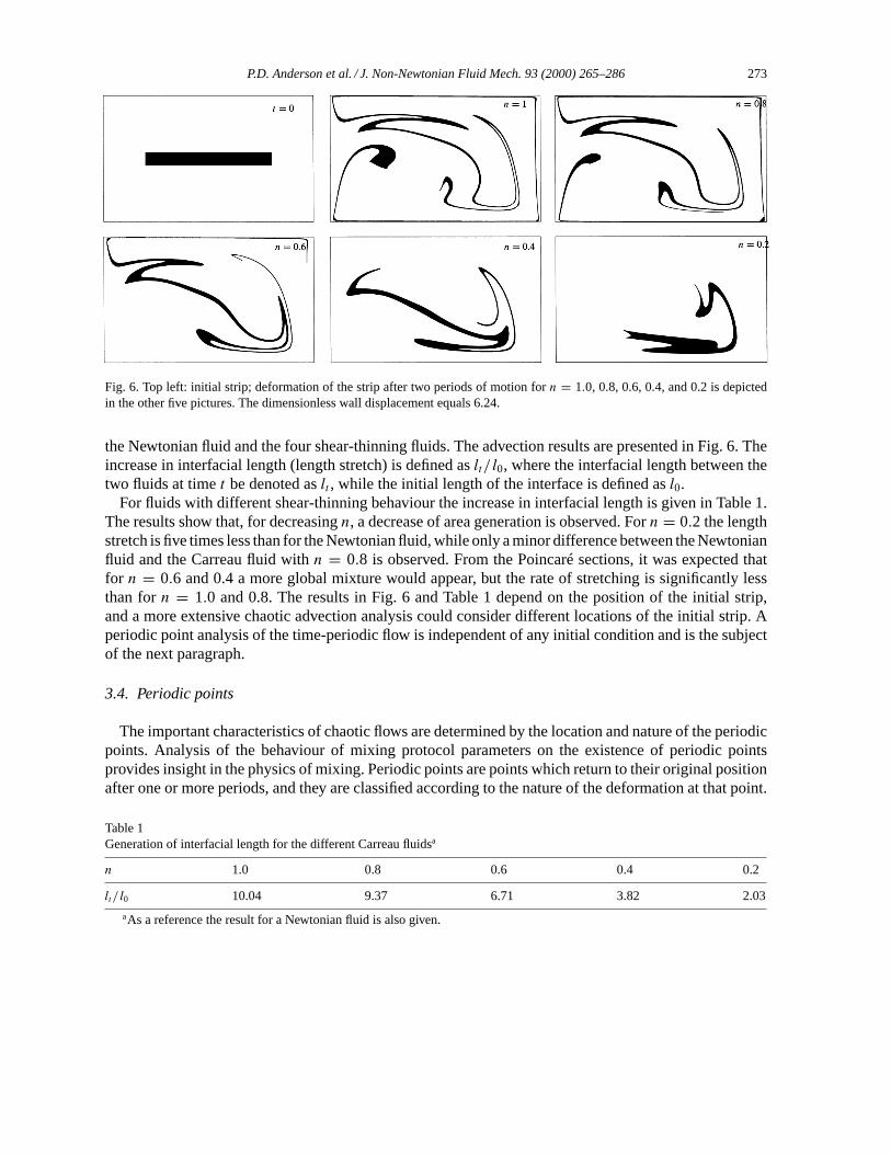
Fig. 6. Top left: initial strip; deformation of the strip after two periods of motion forn = 1.0, 0.8, 0.6, 0.4, and 0.2 is depictedin the other five pictures. The dimensionless wall displacement equals 6.24.

the Newtonian fluid and the four shear-thinning fluids. The advection results are presented in Fig. 6. Theincrease in interfacial length (length stretch) is defined aslt / l0, where the interfacial length between thetwo fluids at timet be denoted aslt , while the initial length of the interface is defined asl0.

For fluids with different shear-thinning behaviour the increase in interfacial length is given in Table 1.The results show that, for decreasingn, a decrease of area generation is observed. Forn = 0.2 the lengthstretch is five times less than for the Newtonian fluid, while only a minor difference between the Newtonianfluid and the Carreau fluid withn = 0.8 is observed. From the Poincaré sections, it was expected thatfor n = 0.6 and 0.4 a more global mixture would appear, but the rate of stretching is significantly lessthan forn = 1.0 and 0.8. The results in Fig. 6 and Table 1 depend on the position of the initial strip,and a more extensive chaotic advection analysis could consider different locations of the initial strip. Aperiodic point analysis of the time-periodic flow is independent of any initial condition and is the subjectof the next paragraph.

3.4. Periodic points

The important characteristics of chaotic flows are determined by the location and nature of the periodicpoints. Analysis of the behaviour of mixing protocol parameters on the existence of periodic pointsprovides insight in the physics of mixing. Periodic points are points which return to their original positionafter one or more periods, and they are classified according to the nature of the deformation at that point.

Table 1Generation of interfacial length for the different Carreau fluidsa

n 1.0 0.8 0.6 0.4 0.2

lt / l0 10.04 9.37 6.71 3.82 2.03

aAs a reference the result for a Newtonian fluid is also given.


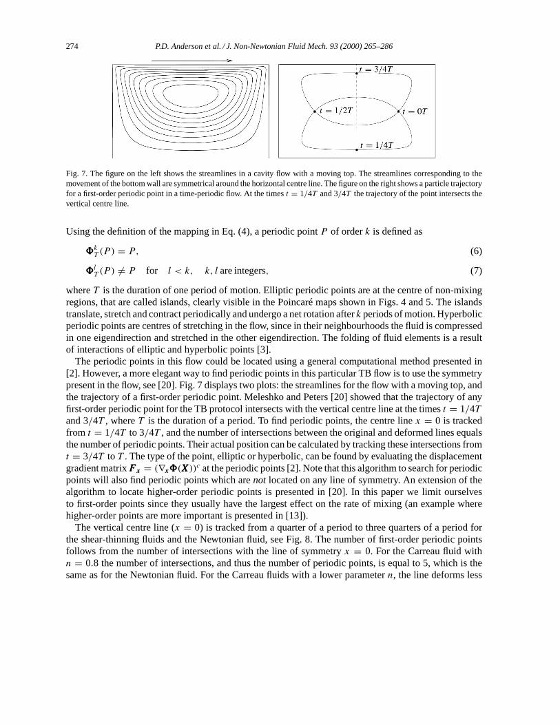
Fig. 7. The figure on the left shows the streamlines in a cavity flow with a moving top. The streamlines corresponding to themovement of the bottom wall are symmetrical around the horizontal centre line. The figure on the right shows a particle trajectoryfor a first-order periodic point in a time-periodic flow. At the timest = 1/4T and 3/4T the trajectory of the point intersects thevertical centre line.

Using the definition of the mapping in Eq. (4), a periodic pointP of orderk is defined as

888kT (P ) = P, (6)

888lT (P ) 6= P for l < k, k, l are integers, (7)

whereT is the duration of one period of motion. Elliptic periodic points are at the centre of non-mixingregions, that are called islands, clearly visible in the Poincaré maps shown in Figs. 4 and 5. The islandstranslate, stretch and contract periodically and undergo a net rotation afterk periods of motion. Hyperbolicperiodic points are centres of stretching in the flow, since in their neighbourhoods the fluid is compressedin one eigendirection and stretched in the other eigendirection. The folding of fluid elements is a resultof interactions of elliptic and hyperbolic points [3].

The periodic points in this flow could be located using a general computational method presented in[2]. However, a more elegant way to find periodic points in this particular TB flow is to use the symmetrypresent in the flow, see [20]. Fig. 7 displays two plots: the streamlines for the flow with a moving top, andthe trajectory of a first-order periodic point. Meleshko and Peters [20] showed that the trajectory of anyfirst-order periodic point for the TB protocol intersects with the vertical centre line at the timest = 1/4T

and 3/4T , whereT is the duration of a period. To find periodic points, the centre linex = 0 is trackedfrom t = 1/4T to 3/4T , and the number of intersections between the original and deformed lines equalsthe number of periodic points. Their actual position can be calculated by tracking these intersections fromt = 3/4T to T . The type of the point, elliptic or hyperbolic, can be found by evaluating the displacementgradient matrixFFFxxx = (∇xxx888(XXX))c at the periodic points [2]. Note that this algorithm to search for periodicpoints will also find periodic points which arenot located on any line of symmetry. An extension of thealgorithm to locate higher-order periodic points is presented in [20]. In this paper we limit ourselvesto first-order points since they usually have the largest effect on the rate of mixing (an example wherehigher-order points are more important is presented in [13]).

The vertical centre line (x = 0) is tracked from a quarter of a period to three quarters of a period forthe shear-thinning fluids and the Newtonian fluid, see Fig. 8. The number of first-order periodic pointsfollows from the number of intersections with the line of symmetryx = 0. For the Carreau fluid withn = 0.8 the number of intersections, and thus the number of periodic points, is equal to 5, which is thesame as for the Newtonian fluid. For the Carreau fluids with a lower parametern, the line deforms less


Fig. 8. Deformation of the linex = 0 from t = 1/4T to 3/4T for five different fluids. The number of intersections with theoriginal line reveals the number first-order periodic points. Note that, for computational reasons, the initial centre line does nottouch the upper and lower walls.

and, as a result, the number of periodic points is only three. Obviously periodic points ‘collapse’ ifn

is decreased fromn = 0.8 to 0.6. For the flow with fluid parametern = 0.2 only one single (elliptic)periodic point remains. The decrease in number of first-order periodic points, caused by reduction inshear-rate magnitude, usually results in a decrease of local mixing efficiency, since hyperbolic periodicpoints, which account for repetitive high stretching in mixing flows, may be lost.

A similar effect as shown in Fig. 8 is observed when the rheology of the fluid is fixed and the dimen-sionless displacement parameterD is decreased. However, the differences in mixing behaviour for theNewtonian and shear-thinning fluids cannot be all attributed to a reduction of an effective dimensionlessdisplacement parameter. This will become clear in the following Section 3.5.

3.5. Application of the ‘mapping’ method

The methods applied in the previous sections discuss details of mixing, and have proven to be eleganttools to analyse the chaotic behaviour of mixing flows. In principle it is possible to obtain all the relevantinformation on the behaviour of a mixing protocol, and analyse whether it may lead to (global) chaoticmixing. Since these techniques are relatively expensive, it is computationally impossible to qualitativelyor quantitatively compare a large number of different mixing protocols, or even a single mixing protocolfor different dimensionless displacements. Optimisation of mixing is thus impractical. To answer thisquestion a more flexible and efficient technique is necessary and introduced in the next sub-section.

3.5.1. The techniqueThe ‘mapping’ method is proposed based on the original ideas of Spencer and Wiley [28], and the idea

is not to track each material volume in the flow domain separately, but to create a discretised mappingfrom a reference grid to a deformed grid. Instead of tracking the boundaries of material volumes a setof distribution matrices are used to advect concentration in the flow. Within the mapping method a flowdomain�� is subdivided intoN non-overlapping sub-domains��i with boundaries∂��i . The boundaries


Fig. 9. (Left) Initial sub domain discretisation (10× 6 grid) and (right) deformed grid after displacement of the top wall by twotimes its length. During the actual computations a finer 200× 120 grid was used.

∂��i of these sub-domains, represented by polygons, are tracked in a flow fromt = t0 to t0 + 1t usingan adaptive front tracking model [10], and result in deformed polygons. The subdivision of�� into ��i ’sis not related to any finite differences, or finite element discretisation used to solve the velocity fieldin �. Next, a discretised mapping from the initial grid to the deformed grid is constructed, see Fig. 9.The distribution of, for example, fluid concentration in the original grid is then mapped to obtain a newdistribution.

The area of the intersections of the deformed sub-domains with the original ones, determine the elementsof the mapping (or distribution) matrix9, where9ij equals the fraction of the deformed sub-domain��j

at timet = t0 + 1t that is found in the original (t = t0) sub-domain��i

9ij =∫��j |t=t0+1t∩��i |t=t0

d��∫��j |t=t0

d��. (8)

The polygonal descriptions of the sub-domains are used to determine the matrix elements9ij , and theaccuracy of these elements is determined by the accuracy of the velocity field and the error tolerancesdefined in the adaptive front tracking procedure. Note that the matrix9 is essentially sparse if1t is nottoo large [14].

The computation of the matrix elements9ij is time consuming (more than 100 h using a 12 CPUmultiprocessor 225 MHz R10K Silicon GraphicsTM) for the shear-thinning examples presented laterin this section. However, once the matrices are obtained, matrix–vector multiplications are extremelyfast (less than 1 s on a single CPU 100 MHz PentiumTM). The combination of a number of matricesfor different wall displacement parametersD are used in [14] to compare different Newtonian mixingprotocols. For potential ‘optimal’ mixing protocols, mixing efficiency diagrams are created, which canbe used to choose an optimal dimensionless displacement parameter. Here this technique is appliedto investigate the influence of shear-thinning behaviour on mixing for a wide range of the flow para-meterD.

The quantity being mapped here, as an example, is the averaged concentration of a marker fluid, whichis rheologically identical to the matrix fluid. The distribution of the marker fluid is described by a columnvectorCCC, and its componentsCi are the locally averaged concentrations in each sub-domain��i . If the


initial distribution att0 = 0 is described by the concentration vectorCCC0, the concentration after time1t can be computed asCCC1t = 9CCC0. An initial condition can be a strip of fluid like in Fig. 6, or forexample, the cavity is filled with half white and half black fluid. If the same flow is continued (repetitivemixing), the concentration afterk steps isCCCk1t = 9kCCC0. Spencer and Wiley [28] suggested to analysemixing behaviour by studying9k. However, this is not feasible for high spatial resolution. In this casethe matrix9k will not be sparse for largek, because fluid from every sub-domain is advected into most,or even all, of the other sub-domains. Instead of studying9k, the evolution of the vectorCCCk is studied.The concentration vectorCCCk is computed in a sequence

CCCi+1 = 9CCCi, (9)

without a direct evaluation of9k. A simple quantitative criterion to characterise the degree of ‘mixedness’is needed to describe the mixed state. A useful characteristic, which is called ‘discrete intensity ofsegregation’, is defined as

I = 1

c(1 − c)

1

A

N∑

i=1

(ci − c)2ai, where c = 1

A

N∑

i=1

ciai, A =N∑

i=1

ai. (10)

The sum is computed over all internal cells,N is the number of cells,ci the concentration of the markerfluid in the celli that has the areaai , A the total area of all cells taken into account, andc is the averageconcentration of marker fluid in��. As the grids used in this work are regular and all their cells have equalvolumes, formula (10) can be simplified to

I = 1

c(1 − c)

1

N

N∑

i=1

(ci − c)2, with c = 1

N

N∑

i=1

ci. (11)

The definition of the mixing measureI is similar to the standardintensity of segregationas introducedby Danckwerts [9]. Similar measures were used by Tucker [30]. Unlike the intensity of segregation, thediscrete intensity of segregation is defined through the concentration averaged in the finite sized cells,and not via the integral over point-wise values of concentration. Note that 0≤ I ≤ 1 and forI = 0 themixture is ideal;I = 1 represents an unmixed state.

3.5.2. Mapping results for two-dimensional flowThe mapping technique was applied for the top–bottom, i.e. TB mixing protocol as studied earlier.

The mapping matrix is constructed on the 200× 120 grid defined on the domain��m : δ × h ≤ x ≤δ × h, −δ ≤ y ≤ δ, where the factorδ = 0.985 is used for computational reasons. The geometric cornerand boundary singularities of the cavity flow result in infinite polymer stresses, and particle paths close tothe corners lead to unacceptable long program runs (ifδ → 1). Therefore, the excluded domain�� \ ��m

is treated as a single cell in the mapping matrix. Mapping matrices are constructed withD = 0.25, 1, 2,and 4, whereT is again the duration of one period of motion. It should be noted that numerical diffusionis introduced as a side effect of the mapping method, and the amount of diffusion is determined by thegrid size, the size of the domain�� \ ��m, and the number of subsequent mapping steps needed. As aresult the minimum intensity of segregation is here of the order 10−3. In [14] some modifications in thecomputation of the mapping matrix are proposed, which makes it possible to use finer grids and as aresult significantly lower values of the intensity of segregation are reached.


The initial distribution of fluid which is mixed is as follows: black fluid (C = 1) is placed in the left halfof the cavity, while in the other half of the cavity white fluid (C = 0) is placed. The fluids are mixed usingthe mixing protocol TB for a large number of values of the mixing parameterD. Discrete intensity ofsegregation, as introduced in Eq. (11), is used as a mixing measure. For some dimensionless displacementsresults are presented in Fig. 10 for the Newtonian fluid and the Carreau fluids with power-law parametern = 0.6 and 0.2. The Carreau number, Cr, is fixed and equals 5. The total number of wall movements, adirect measure for the energy input, is equal for all these plots and equals 32, i.e. we compare 16 timesa D = 2 wall displacement, with eight timesD = 4, four timesD = 8, two timesD = 16, and onestep ofD = 32. Horizontally the influence of the power-law parameter is compared. For this relativelysmall number of wall movements it is observed that the Newtonian fluid mixes better than the Carreaufluid with n = 0.6, which again mixes better than the Carreau fluid withn = 0.2. Moreover, further onin Figs. 11 and 12 it is, however, concluded that if more wall displacements are applied, shear-thinningbehaviourcan lead to better mixing.

For the same three fluids (n = 1, 0.6, 0.2) mixing efficiency plots are computed. These plots areconstructed by considering fluid mixing for a large number of combinationsk×D, wherek is the numberof wall movements, and plotting the discrete intensity of segregation. The maximum dimensionlessdisplacement was equal to 16, and the number of wall movements is limited to 32. To construct each ofthe mixing efficiency diagrams presented in Fig. 11, a total of 8192 mixing simulations are performedusing the mapping approach. The picture on the top of Fig. 11 shows the results for the Newtonian fluid,while the other two plots shows the results for the Carreau fluids. White regions correspond to parametersubsets leading to efficient mixing; dark regions correspond to poor mixing parameter settings.

The Newtonian results in Fig. 11 show a number of intervals forD of low and high intensity ofsegregation. For 0≤ D ≤ 4 the plot shows that the mixing quality is poor, and even for an extreme largenumber of wall movements, beyond the range of this figure, mixing remains poor. For a somewhat largerdimensionless displacement ofD, where 4≤ D ≤ 5.5, mixing becomes considerably more efficient. Inthe range of 5.5 ≤ D ≤ 9 a poorer mixing quality results, but again increasing the parameterD to 10leads to more efficient mixing zone again. BetweenD = 10 and 12 a third zone of less efficient mixingis visible, which transfers to the chaotic zone 12≤ D ≤ 16.

As a result of the shear-thinning behaviour of the Carreau fluidsn = 0.6 and 0.2 shifts in the corre-sponding mixing efficiency diagrams are observed. Decreasing the power-law parametern enlarges theminimum dimensionless displacement required to obtain a nearly global chaotic mixing flow. For thestrongest shear-thinning fluid, displacement steps ofD = 8 are required to get good mixing. The zonesof good and bad mixing as found for the Newtonian fluid are also observed for the non-Newtonian fluids,but the streaks appear to be wider.

A more clear comparison of the mixing behaviour of the three fluids is given in Fig. 12. Here intensity ofsegregation is plotted as a function of number of wall displacements for afixeddimensionless displacementparameter. ForD = 2 mixing quality is very poor for all three fluids, as expected from the (morequalitative) results shown in Fig. 11. ForD = 6 it is first observed that shear-thinning fluids can leadto better mixing than in the Newtonian case. Here, the curve forn = 0.6 is below the Newtonian curve,which again is below then = 0.2 curve. In this case a large island is present for the Newtonian fluid(see Fig. 4), and obviously also forn = 0.2. If D is increased toD = 8 results are inverted and theCarreau fluid withn = 0.2 leads to the most efficient mixing. Already after 30 wall displacements theintensity of segregation is orders lower than for the fluids withn = 0.6 and 1.0. ForD = 12 the weakershear-thinning fluid leads to better mixing, where for the strong shear-thinning fluid the intensity of


Fig. 10. Mixing patterns for the Newtonian (left) and the two shear-thinning fluids (middle and right). The initial distributionof fluid is as follows: black fluid (C = 1) is placed in the left half of the cavity, while in the other half of the cavity white fluid(C = 0) is placed.


Fig. 11. Mixing quality plots for a Newtonian (top) and shear-thinning Carreau fluid withn = 0.6 (middle) and a Carreau fluidwith power-law parametern = 0.2 (bottom). The Carreau number equals five in all cases. Grey values denote different valuesfor (1 − I); black represents bad mixing. The dashed hyperbolic contours represent lines of equal energy input.


Fig. 12. Mixing quality plots for the Newtonian and two shear-thinning fluids for a constant dimensionless wall displacement.

segregation is bounded by approximately 1× 10−3. Increasing toD = 14 shows that the Newtonianfluids has the largest rate of mixing, and only after eight wall displacements the lower limit of intensityof segregation is reached. Note that in Fig. 12, the total energy input in the mixing process is, at a fixednumber of wall displacements, linearly proportional toD.


4. Three-dimensional cavity flows

As far as known to the authors, no studies have been reported in the literature on the analysis ofthree-dimensional non-Newtonian mixing flows focusing on the behaviour of periodic points. The mixingprotocol studied here is a straightforward extension of the protocol for the two-dimensional cavity usedin the preceding section, and consists of a time-periodic motion of the front and back wall. All other wallsare stationary. As a result of the lid and bottom of the cavity, three-dimensional effects are expected. Thedimensionless displacementD equals 7, similar to the Newtonian results presented in [2].

Similar computational techniques as used for the two-dimensional problem are applied to obtain thevelocity field in the three-dimensional cavity. The flow domain is subdivided in 6× 8 × 6 spectralelements each of sixth order. The computed Newtonian velocity is again taken as an initial field toobtain the shear-thinning velocity fields. In principle it is possible to construct a Poincaré map for athree-dimensional cavity flow, and analyse the mixing behaviour similar as done for the two-dimensionalproblems. However, the outcome is less simple to use since the resulting set of points is located in thethree-dimensional cavity and regions of bad mixing are less easy detected. Therefore, we will go directlyto the core of the problem and study the influence a shear-rate dependent viscosity on first-order periodicpoints for the TB protocol.

Periodic points are located for three different Carreau fluids with power-law parametersn = 0.9, 0.7,and 0.6 (this range is considered here, since an interesting transition in mixing quality is observed aroundn = 0.65). The technique applied to locate the periodic points is similar to the two-dimensional case with

Fig. 13. Periodic lines from shear-thinning fluids with power-law parametersn = 1.0, 0.9, 0.7, and 0.6.


the difference that here a two-dimensional plane located at the plane of symmetry is tracked from a quarterto three quarters of a periodic. The intersection of the deformed and the original plane determines the setof periodic points. The type of the first-order periodic points is determined by studying the eigenvaluesof the displacement gradient matrix at the periodic points.

Similar to results discussed in [2] the sets of periodic points form periodic lines, and the nature of theperiodic points can change along each line. The results are displayed in Fig. 13, where the set of linescorresponding to the Newtonian fluid are added as a reference. The thin lines are of hyperbolic type,whereas the thick lines are of elliptic type. Symmetry, which is present for this flow, is also revealed bythe periodic points. The planes of symmetry are the mid-planez = 0.5 and the planey = 0. It appearsthat within this range periodic points collapse (for decreasingn) and that the type of a periodic point maychange. The front view of Fig. 13 shows that forn = 0.9 periodic lines are still present in the left halfof the cavity; for the lowern parameters these lines disappear. The side view picture clearly shows that,for a decreasingn, the length of the lines decreases and the type changes along the line. Forn = 0.6 thelines are almost completely elliptic. From these results it is expected that the mixing in this cavity flowwill be poorer for shear-thinning fluids. If the power-law indexn would be decreased further, the set ofthree periodic lines would eventually collapse and a single (elliptic) periodic line remains.

To demonstrate the influence of the parametern on mixing, a blob is advected in the flow for fourperiods of motion. The initial blob is located such that it touches the periodic lines forn = 0.6 and 0.7,

Fig. 14. Deformation after four periods of a blob positioned between periodic lines belonging to different shear-thinning pa-rameters. The centre of the blob lies on the periodic line forn = 0.65, while the radius of the blob is chosen such that the blobtouches the periodic lines forn = 0.6 and 0.7.


see Fig. 14. A large difference in the advection of the blob is observed. For the Carreau fluid withn = 0.7the blob is stretched and folded more extensively than forn = 0.6. Such an outcome is not surprising,since the periodic points in this region are hyperbolic forn = 0.7 but elliptic forn = 0.6. These resultsshow that the mixing behaviour can locally be very sensitive to the rheological properties of the fluid. Anatural route to extend the three-dimensional analysis would be the development and application of themapping method, and to study the influence of dimensional wall displacement on the mixing quality forthe different shear-thinning fluids. This is the subject of future research.

5. Summary and conclusions

This paper deals with a Carreau shear-thinning viscosity model to study mixing characteristics ofnon-Newtonian fluids. To obtain the corresponding velocity fields for a two- and three-dimensionalcavity flow, computational methods are used to study the inelastic non-Newtonian effects. Even thoughthe deviations from the Newtonian flow of steady-state velocity fields are relatively small, large effects areobserved in the chaotically advected patterns in the time-periodic two- and three-dimensional flows. Ingeneral, for the systems studied in this work, the overall effect of a shear-thinning viscosity is a decreasein the rate and extent of mixing. The shear-thinning viscosity results in a decrease of stretching in theflow, a primary route to efficient mixing.

For the two-dimensional flows, it is shown that hyperbolic (unstable) periodic points disappear ifshear-thinning is increased, or they transform into elliptic (stable) periodic points. For the three-dimensionalflows, similar effects are observed for the set of periodic lines present in the cavity. The length of thelines decreases if shear-thinning is increased, and the nature of parts of these lines change from hy-perbolic to elliptic. The overall effect is again a decrease in the rate of mixing. Shear-thinning be-haviour of the fluid can, however, lead to a more global mixture (also observed by Niederkorn and Ottino[22]), and for the two-dimensional system several examples are provided. Similarly, mixing behaviour inthree-dimensional shear-thinning flows can be (locally) very sensitive to rheological fluid parameters, andfuture work is focused to study global effects on mixing using a three-dimensional version of the mappingmethod.

The application of the two-dimensional mapping method for different fluids, makes a comparison ofmixtures possible for a much larger variation of parameters. In mixing efficiency diagrams the resultsare easily quantitatively compared and parameter zones of good and bad mixing are separated. From theplots it is immediately clear that zones of good mixing found for a Newtonian fluid, can be zones ofbad mixing for a shear-thinning fluid or vice versa. The non-Newtonian behaviour of the fluid not onlyleads to a shift of these zones, since some of them increase in width, while other zones become morenarrow. Hence, the differences cannot be only attributed to a reduced shear-rate magnitude. The resultssummarised in this paper clearly show the (possible) influence of changes in the rheology of the fluid onthe mixing properties. Moreover, examples are given where mixing may become either better or worsecompared to the Newtonian system.

Future research will study elastic effects in mixing. For Boger fluids we can study pure elastic effects andcompare with the Newtonian results. For viscoelastic flows with shear-thinning behaviour a comparisonwith the shear-thinning results presented in this paper is possible. Moreover, an experimental setup ofa three-dimensional cavity flow is currently built in our laboratory and will be used to validate resultspresented here.


Acknowledgements

The authors would like to acknowledge support by the Dutch Foundation of Technology (STW), GrantNo. EWT44.3453, and the Dutch Polymer Institute (DPI), Project No. 161.

References

[1] P. Anderson, Computational Analysis of Distributive Mixing, Ph.D. thesis, Eindhoven University of Technology, TheNetherlands, 1999.

[2] P. Anderson, O. Galaktionov, G. Peters, F. van de Vosse, H. Meijer, Analysis of mixing in three-dimensional time-periodiccavity flows, J. Fluid Mech. 386 (1999) 149–166.

[3] P. Anderson, O. Galaktionov, G. Peters, F. van de Vosse, H. Meijer, Chaotic fluid mixing in non-quasi-static time-periodiccavity flows, Int. J. Heat Fluid Flow 21 (2) (2000) 176–185.

[4] H. Aref, Stirring by chaotic advection, J. Fluid Mech. 143 (1984) 1–21.[5] F. Baaijens, Mixed finite element methods for viscoelastic flow analysis: a review, J. Non-Newtonian Fluid Mech. 79 (1998)

361–385.[6] D. Bigg, S. Middleman, Mixing in a screw extruder: a model for residence time distribution and strain, Ind. Eng. Chem.

Fundam. 13 (1974) 66–71.[7] J. Chaiken, R. ad Chevray, M. Tabor, Q. Tan, Experimental study of Lagrangian turbulence in Stokes flow, Proc. R. Soc.,

London A408 (1986) 165–174.[8] W. Chien, H. Rising, J. Ottino, Laminar mixing and chaotic mixing in several cavity flows, J. Fluid Mech. 170 (1986)

355–377.[9] P. Danckwerts, The definition and measurement of some characteristics of mixtures, Appl. Sci. Res. Sec. A (1952).

[10] O. Galaktionov, P. Anderson, G. Peters, F. van de Vosse, An adaptive front tracking technique for three-dimensional transientflows, Int. J. Numer. Meth. Fluids 32 (2) (2000) 201–217.

[11] A. Grillet, B. Yang, B. Khomami, E. Shaqfeh, Modeling of viscoelastic lid driven cavity flow using finite element simulations,J. Non-Newtonian Fluid Mech. 88 (1/2) (2000) 99–132.

[12] M. Hirsch, S. Smale, Differential Equations, Dynamical Systems, and Linear Algebra, Academic Press, London, 1974.[13] S. Jana, G. Metcalfe, J. Ottino, Experimental and computational studies of mixing in complex Stokes flows: the vortex

mixing flow and multicellular cavity flows, J. Fluid Mech. 269 (1994) 199–246.[14] P. Kruijt, O. Galaktionov, P. Anderson, G. Peters, H. Meijer, Analyzing fluid mixing in periodic flows by distribution

matrices, AIChE J., 2000, submitted for publication.[15] S. Kumar, G. Homsy, Chaotic advection in creeping flow of viscoelastic fluids between slowly modulated eccentric cylinders,

Phys. Fluids 8 (1996) 1774–1787.[16] C. Leong, J. Ottino, Increase in regularity by polymer addition during chaotic mixing in two-dimensional flows, Phys. Rev.

Lett. 64 (8) (1990) 874–877.[17] C. Leong, J. Ottino, Experiments on mixing due to chaotic advection in a cavity, J. Fluid Mech. 209 (1989) 463–499.[18] F. Ling, X. Zhang, Mixing of a generalized Newtonian fluid in a cavity, J. Fluids Eng. 117 (1995) 75–117.[19] Y. Maday, A. Patera, Spectral element methods for the incompressible Navier–Stokes equations, in: A. Noor (Ed.),

State-of-the-Art Surveys on Computational Mechanics, ASME, New York, 1989.[20] V. Meleshko, G. Peters, Periodic points for two-dimensional Stokes flow in a rectangular cavity, Phys. Lett. A 216 (1996)

87–96.[21] T. Niederkorn, J. Ottino, Mixing of a viscoelastic fluid in a time-periodic flow, J. Fluid Mech. 256 (1993) 243–268.[22] T. Niederkorn, J. Ottino, Chaotic mixing of shear-thinning fluids, AIChE J. 40 (11) (1994) 1782–1793.[23] J. Ottino, The Kinematics of Mixing: Stretching, Chaos and Transport, Cambridge University Press, Cambridge, 1989.[24] G.P.J. Schoonen, F. Baaijens, H. Meijer, On the performance of enhanced constitutive models for polymer melts in a

cross-slot flow, J. Non-Newtonian Fluid Mech. 82 (1999) 387–427.[25] W. Press, S. Teukolsky, W. Vetterling, B. Flannerly, Numerical Recipes infortran, 2nd Edition, Cambridge University

Press, Cambridge, 1992.[26] J. Schoonen, Determination of rheological constitutive equations using complex flows, Ph.D. thesis, Eindhoven University

of Technology, The Netherlands, 1998.


[27] A. Souvaliotis, S. Jana, J. Ottino, Potentialities and limitations of mixing simulations, AIChE J. 41 (7) (1995) 1605–1621.[28] R. Spencer, R. Wiley, The mixing of very viscous liquids, J. Colloid Sci. 6 (1951) 133–145.[29] L. Timmermans, P. Minev, F. van de Vosse, An approximate projection scheme for incompressible flow using spectral

elements, Int. J. Numer. Meth. Fluids 22 (1996) 673–688.[30] C. Tucker, Principles of mixing measurement, in: C. Rauwendaal (Ed.), Mixing in Polymer Processing, Plastics Engineering,

Marcel Dekker, New York, 1991.[31] S. Unverdi, G. Tryggvason, A front-tracking method for viscous, incompressible multi-fluid flows, J. Comp. Phys. 100

(1992) 25–37.

Mixing of non-Newtonian fluids in time-periodic cavity flows

Documents

Transcript of Mixing of non-Newtonian fluids in time-periodic cavity flows