Minimizing the Delta Testfor Variable Selection inRegression Problems

A. Guillen*Department of Computer Architecture and Technology,University of Granada, SpainE-mail: aguillen@atc.ugr.es*Corresponding author

D. SoviljDepartment of Information and Computer Science,Helsinki University of Technology, FinlandE-mail: dusans@cis.hut.fi

F. MateoInst. of Applications of Information Technology and Advanced Communications,Polytechnic University of Valencia, SpainE-mail: fermaji@upvnet.upv.es

I. Rojas and A. LendasseDepartment of Computer Architecture and Technology,University of Granada, SpainE-mail: irojas@atc.ugr.esDepartment of Information and Computer Science,Helsinki University of Technology, FinlandE-mail: lendasse@hut.fi

Abstract: The problem of selecting an adequate set of variables from a given dataset of a sampled function, becomes crucial by the time of designing the model thatwill approximate it. Several approaches have been presented in the literature althoughrecent studies showed how the Delta Test is a powerful tool to determine if a subset ofvariables is correct. This paper presents new methodologies based on the Delta Testsuch as Tabu Search, Genetic Algorithms and the hybridization of them, to determinea subset of variables which is representative of a function. The paper considers aswell the scaling problem where a relevance value is assigned to each variable. The newalgorithms were adapted to be run in parallel architectures so better performances couldbe obtained in a small amount of time, presenting great robustness and scalability.

Keywords: Variable selection; delta test; forward-backward search; tabu search; ge-netic algorithms; hybrid algorithms; parallel architectures.

Reference to this paper should be made as follows: Guillen, A., Sovilj, D., Mateo, F.,Rojas, I. and Lendasse, A. (200?) ‘New methodologies based on delta test for variableselection in regression problems’, Int. J. High Performance Systems Architecture, Vol.?, No. ?, pp.?–?.

Biographical notes: Fernando Mateo is a MSc researcher pursuing his PhD at theInstitute of Applications of Information Technology and Advanced Communications,in the Polytechnic University of Valencia, Valencia, Spain. He obtained his M.Sc. fromthe Polytechnic University of Valencia in 2005. Since then, he has been researchingin machine learning methods and their applications, namely: Position estimation inPET detectors, prediction of contaminants in food and variable selection techniquesfor high-dimensional problems.

1 INTRODUCTION

In many real-life problems it is convenient to reduce thenumber of involved features (variables) in order to reducethe complexity, especially when the number of features islarge compared to the number of observations (e.g. fi-nance problems, weather forecast, electricity load predic-tion, medical or chemometric information, etc.). There areseveral criteria to tackle this variable reduction problem.Three of the most common are: maximization of the mu-tual information (MI) between the inputs and the outputs,minimization of the k-nearest neighbors (k-NN) leave-one-out generalization error estimate and minimization of anonparametric noise estimator (NNE).

The problem of regression or function approximationconsists in, given a set of input vectors with their corre-sponding output, it is desired to build a model that learnsthe relationship between the input variables and the out-put variable. The designed model should also have theability to generalize, so when new input vectors that werenot in the original training data set are given to the model,it is able to generate the correct output for those values.Formally this problem can be enunciated as, given a set ofobservations {(~xj ; yj); j = 1, ..., N} with yj = F (~xj) ∈ R

and ~xj ∈ Rd, it is desired to obtain a function G so yj = G

(~xj) ∈ R with ~xj ∈ Rd.

There exists a wide variety of models that are able toapproximate any function such as Radial Basis FunctionNeural Networks (Poggio and Girosi, 1989), MultilayerPerceptrons (Rosenblatt, 1958), Fuzzy Systems (Kosko,1994), Gaussian Process (Rasmussen, 2004), Support Vec-tor Machines (SVM) and Least Square SVM (Lee andVerri, 2002), etc. however, they all suffer from the Curseof Dimensionality (Herrera et al., 2006). As the number ofdimensions d grows, the number of input values requiredto sample the solution space increases exponentially, thismeans that the models will not be able to set their param-eters correctly if there are not enough input vectors in thetraining set. Many real life problems present this draw-back since they have a considerable amount of variablesto be selected in comparison to the few number of obser-vations. Thus, efficient and effective algorithms to reducethe dimensionality of the data sets are required. Anotheraspect that is improved by selecting a subset of variables isthe interpretability of the designed systems (Guyon et al.,2006).

The literature presents a wide number of methodologiesfor feature or variable selection ((Punch et al., 1993; Ohet al., 2004, 2002; Raymer et al., 2000; Saeys et al., 2007))although they have been focused on classification prob-lems. Regression problems differ from classification since:

• the output of the problem is continuous, not likein classification, where a finite number of classes isdefined a priori. For example, the output of thefunction could be in the interval [0,1] meanwhile aclassification could consist in the distinction between

Copyright c© 200x Inderscience Enterprises Ltd.

(table, chair, library).

• There is a proximity between different outputs, notlike in classification, where classes (in general) cannotbe related. For example, it is possible to determinethat the output value 0.45 is closer to 0.5 than thevalue 0.35 but it is not possible to determine a prox-imity between the class table and the class chair orlibrary.

Therefore, specific algorithms for this kind of problemmust be designed. Recently, it has been demonstrated in(Eirola et al., 2008) how the Delta Test (DT) is a quitepowerful tool to determine the quality of a subset of vari-ables. The latest work related to feature selection using theDT consisted in the employment of a local search techniquesuch as Forward-Backward. However, there are other alter-natives that allow to perform a global optimization of thevariable selection like Genetic Algorithms (GA) (Holland,1975) and Tabu Search (TS) (Glover and Laguna, 1997).One of the main drawbacks of using global optimizationtechniques is their computational cost. Nevertheless, thelatest advances in computer architecture provide powerfulclusters without requiring a large budget, so an adequateparallelization of these techniques might ameliorate thisproblem. This is quite important in real life applicationswhere the response time of the algorithm must be accept-able from the perspective of a human operator. This pa-per presents several new approaches to perform variableselection using the DT as criterion to decide if a subsetof variables is adequate or not. The new approaches arebased in local search methodologies, global optimizationtechniques and the hybridization of both. The rest of thepaper is structured as follows: Section 2 introduces the DTand its theoretical framework, then, Section 3 describes theprevious methodology to perform the variable selection aswell as the new developed algorithms. Section 4 presentsa complete experimental study analyzing the behavior ofthe algorithms and, in Section 5, conclusions are drawn.

2 THE DELTA TEST

The Delta Test (DT), firstly introduced by Pi and Peter-son for time series (Pi and Peterson, 1994) and proposedfor variable selection in (Eirola et al., 2008), is a tech-nique to estimate the variance of the noise, or the meansquared error (MSE), that can be achieved without over-fitting. Given N input-output pairs (xi, yi) ∈ R

d × R, therelationship between xi and yi can be expressed as

yi = f(xi) + ri, i = 1, ..., N

where f is the unknown function and r is the noise. TheDT estimates the variance of the noise r.

The DT is useful for evaluating the nonlinear correlationbetween two random variables, namely, input and outputpairs. The DT can be also applied to input variable selec-tion: the set of input variables that minimizes the DT is

2

the one that is selected. Indeed, according to the DT, theselected set of input variables is the one that representsthe relationship between input variables and the outputvariable in the most deterministic way. DT is based onhypothesis coming from the continuity of the regressionfunction. If two points x and x′ are close in the inputvariable space, the continuity of regression function im-plies the outputs f(x) and f(x′) will be close enough inthe output space. Alternatively, if the corresponding out-put values are not close in the output space, this is due tothe influence of the noise.

The DT can be interpreted as a particularization of theGamma Test (Jones, 2004) considering only the first near-est neighbor. Let us denote the first nearest neighbor of apoint xi in the R

d space as xNN(i). The nearest neighborformulation of the DT estimates Var[r] by

Var[r] ≈ δ =1

2N

N∑

i=1

(yi − yNN(i))2,

with Var[δ] → 0 for N → ∞

where yNN(i) is the output of xNN(i).

3 VARIABLE SELECTION METHODOLOGIES

This Section presents the previous methodology proposedto compute the minimum value for the DT, the Forward-Backward search. Then, it presents an adaptation of theTabu search for the minimization of the DT. Finally, a newalgorithm that combines the Tabu Search and the globaloptimization capabilities of GA is introduced.

The methodologies described below are applied to theproblem of variable selection from two perspectives: binaryand scaled. The binary approach considers a solution as aset of binary values that indicate if that variable is relevantor not. The scaled approach assigns a weighting factorto each variable according to its importance. The scalingproblem is more challenging because the solution spacegrows considerably.

3.1 Forward-backward search

To overcome the difficulties and the high computationaltime that an exhaustive search would entail (i.e. 2d − 1input variable combinations, being d the number of vari-ables), there are several other search strategies. Thesestrategies are affected by local optima because they do nottest every input variable combination, but they are pre-ferred over an exhaustive search if the number of variablesis too large.

Among the typical search strategies, there are three thatshare similarities:

• Forward search

• Backward search (or pruning)

• Forward-backward search

The difference between the first two is that the forwardsearch starts from an empty set of selected variables andadds variables to it according to the optimization of asearch criterion, while the backward search starts from aset containing all the variables and removes those for whichthe elimination optimizes the search criterion.

Both forward and backward search suffer from incom-plete search. The Forward-Backward Search (FBS) is acombination of them. It is more flexible in the sense thata variable is able to return to the selected set once it hasbeen dropped, and vice versa, a previously selected vari-able can be discarded later. This method can start fromany initial input variable set: empty set, full set, customset or randomly initialized set. If we consider a set of Ninput-output pairs (xi, yi) ∈ R

d×R, the forward-backwardsearch algorithm can be described as follows

1. Initialization:

Let S be the selected input variable set, which cancontain any input variables, and F the unselectedinput variable set, which contains the variables notpresent in S. Compute Var[r] using Delta Test on theset S.

2. Forward-Backward selection step:

Find the variable xS to include or to remove from theset S to minimize Var[r]:

xS = arg minxi,xj{(Var[r]|S ∪ xj) ∪ (Var[r]|S \ xi)},

xi ∈ S, xj ∈ F

3. If the old value of Var[r] on the set S is lower thanthe new result, stop; otherwise, update set S and savethe new Var[r]. Repeat step 2 until S is equal to anyformer selected S.

4. The selected input variable set is S

3.2 Tabu search

Tabu Search (TS) is a metaheuristic method designed toguide local search methods to explore the solution spacebeyond local optimality. The first most successful usagewas by Glover (Glover, 1986, 1989, 1990) for combinatorialoptimization. Later TS was successfully used in schedul-ing (DellAmico and Trubian, 1993; Mantawy et al., 2002;Zhang et al., 2007), design (Xu et al., 1996a,b), routing(Brandao, 2004; Scheuerer, 2006) and general optimiza-tion problems (Glover, 2006; Hedar and Fukushima, 2006;Al-Sultan and Al-Fawzan, 1997). The TS has become apowerful method with different components tied together,that is able to obtain excellent results in different problemdomains.

In general, the problem is in form of an objective orcost function f(v), given the set of solutions v ∈ V . Inthe context of TS, the neighborhood relationship betweensolutions, denoted Ne(v), plays the central role. While

3

there are other neighborhood based methods, such as de-scent/ascent methods widely used, the difference is thattabu uses memory in order to influence which parts of theneighborhood are going to be explored. A memory is usedto record various aspects of the search process and thesolutions encountered, such as recency, frequency, qual-ity and influence of moves. Instead of storing whole solu-tions in memory, which is impractical in some problems,the common thing is to store attributes of solutions ormoves/operations used to transition from one solution tothe next one.

The most important aspect of the memory is to forbidsome moves to be applied, or in other words, to prevent thesearch to go back to solutions that were already visited.This also allows the search to focus on such moves thatguide the search toward unexplored areas of the solutionsspace. This part of the memory is called a tabu list, andthe moves in this list are then considered tabu, and thusforbidden to use. The size of the tabu list as well as thetime each move is kept in the list are important issues inTS. These parameters should be set up so that the searchis able to go through two distinct, but equally importantphases: intensification and diversification.

As far as we know, no implementation of the TS to min-imize the DT has ever been done, so it was implementedin this work as an improvement over the FBS, which doesnot have any memory enhancement. Due to the fact thatthis paper considers the variable selection and the scal-ing problem, two different algorithms had to be designed.Both algorithms use only short-term recency based mem-ory to store reverse moves instead of solutions to speedupthe exploration of the search space.

3.2.1 TS for pure variable selection

In the case of variable selection, a move was defined as a flipof the status of exactly one variable in the data set. Thestatus is excluded (0) or included (1) from the selection.For a data set of dimensionality d, a solution is then avector of zeros and ones v = (v1, v2, . . . , vd), where vk ∈{0, 1} , k = 1, ..., d, are indicator variables representing theselection status of k-th dimension.

The neighborhood of a selection (solution) v is a setof selections u which have exactly one variable that hasdifferent status. This can be written as

Ne(v) = {u | ∃1q ∈ {1, . . . , d} vq 6= uq ∧ vi = ui, i 6= q}

With this setup, each solution has exactly the sameamount of neighbors, which will be equal to d.

3.2.2 TS for the scaling problem

The first modification that requires the adaptation to thescaling problem is the definition of the neighborhood of asolution. A solution v is now a vector with scaling val-ues from a discretized set vk ∈ H = {0, 1/k, 2/k, . . . , 1},where k is discretization parameter. Two solutions areneighbors if they disagree on exactly one variable, same as

for variable selection, but the disagreement is the small-est possible value. Ne(v) is defined in a same way asfor variable selection, but with an additional constraintof |vq − uq| = 1/k. For example, for k = 10 and d = 3, thesolutions v1 = (0.4, 0.2, 0.8) and v2 = (0.3, 0.2, 0.8) wouldbe neighbors, but not the solution v3 = (0.1, 0.2, 0.8). Themove between solutions is defined as a change of value forone dimension, which can be written as a vector (dimen-sion, old value, new value).

3.2.3 Setting the tabu conditions

The tenure for a move is defined as the number of iter-ations that it is considered as tabu. This value is deter-mined empirically when the TS is applied to solve a con-crete problem. For the variable selection problem, thispaper proposes a value which is dependent on the num-ber of dimensions so it can be applied to several problems.In the experiments, two tabu lists, and thus two tenures,were used. The first list is responsible for preventing thechange along certain dimension for d/4 iterations. The sec-ond one prevents the change along the same dimension andfor specified scaling value for d/4 + 2 iterations. The com-bination of these two lists gave better results than wheneach of the conditions was used alone.

For example, for k = 10, if a move is performed alongdimension 3 from value 0.1 to 0.2, which can be writ-ten as a vector m = (3; 0.1, 0.2), then its reverse movem−1 = (3; 0.2, 0.1) is stored in the list. The search will beforbidden to use any move along dimension 3 for d/4 + 2iterations, and after that time, it will be further 2 itera-tions restricted to use the move m−1, or in other words togo back from 0.2 to 0.1.

With these settings, in the case of variable selection, twoconditions are then implicitly merged into one condition:restrict a flip of the variable for d/4 + 2 iterations. This isbecause there are only two values 0,1 as possible choices.

3.3 Hybrid Parallel Genetic Algorithm

The benefits and advantages of the global optimization andlocal search techniques have been hybridized in the pro-posed algorithm. The idea is to be able to have a globaloptimization, using a GA, but still being able to makea fine tune of the solution, using the TS. The followingparagraphs describe the different elements that define thealgorithm.

3.3.1 Encoding of the individuals and initial pop-

ulation

Deciding how a chromosome encodes a solution is one ofthe most decisive design steps since it will influence therest of the design (De Jong, 1996; Mitchell and Forrest,1995; Michalewicz, 1996). The classical encoding used forvariable selection has been a vector of binary values where1 represents that the variable is selected and 0 that thevariable is not selected. As it has been commented above,

4

this paper is considering the variable selection using scal-ing in order to determine the importance of a variable.Therefore, instead of using binary values, other encodingmust be chosen. If instead of using 0 and 1, the algorithmuses real numbers to determine the weight of a variable,the GA could fall into the category of Real Coded GeneticAlgorithms (RCGA). However, the number of scales hasbeen discretized in order to bound the number of possiblesolutions making the algorithm a classical GA where thecardinality of the alphabet for the solutions is increased ink values. For the sake of simplicity in the implementation,an individual is a vector of integers where the number 1represents that the variable was selected and k + 1 meansthat the variable is not selected.

Regarding the initial population, some individuals areincluded in the population deterministically to ensure thateach scaling value for each variable exists in the population.These individuals are required if the classical GA crossoveroperators (one/two-points, uniform) are applied so all thepossible combinations can be reached. For example, if thenumber of scales is 4 in a problem with 3 variables, theindividuals that are always included in the population are:1 1 1, 2 2 2, 3 3 3, and 4 4 4.

3.3.2 Selection, crossover and mutation operators

The algorithm was designed in order to be as fast as pos-sible so when several design options appeared, the fastestone (in terms of computation time) was selected, as longas it was reasonable. The selection operator chosen wasthe binary tournament selection as presented by Goldbergin (Goldberg, 1989) instead of the Baker’s roulette wheeloperator (Baker, 1987) or other more complex operatorsexisting in the literature (Chakraborty et al., 1996). Thereason for this is because the binary tournament does notrequire the computation of any probability for each in-dividual, thus, a considerable amount of operations aresaved on each iteration. This is specially important forlarge populations. Furthermore, the fact that the binarytournament does not introduce a high selective pressure isnot as traumatic as it might seem. The reason is becausethe huge solution space, that arises as soon as the numberof scales increases, should be deeply explored to avoid lo-cal minima. Nevertheless, the algorithm incorporates theelitism mechanism, keeping the 10% of the best individualsof the population, so the convergence is still feasible.

Regarding the crossover operator, the algorithm imple-mented the classical operators for a binary coded GA, theseare: one-point and two-point crossovers and the uniformcrossover (De Jong, 1975; Holland, 1975; Sywerda, 1989).The behavior of the algorithm using these crossovers wasquite similar and acceptable. Nonetheless, since the algo-rithm could be included into the Real Coded GA class, anadaptation of the BLX-α (Eshelman and Schaffer, 1993)was implemented as well. The operator consists in, giventwo individuals I1 = (i11, i

12, ...i

1d) and I2 = (i21, i

22, ...i

2d)

with (i ∈ R), a new offspring O = (o1, ..., oj , ..., od)can be generated where oj , j = 1...d is a random value

chosen from an uniform distribution within the interval[imin − α · B, imax + α · B] where imin = min(i1j , i

2j),

imax = max(i1j , i2j), B = imax − imin and α ∈ R. The

adaptation only required to round the absolute value as-signed to each gene and also the modification of the valuein case it is out of the bounds of the solution space.

The mutation operates at a gene level, so a gene has thechance to get any value of the alphabet.

3.3.3 Parallelization

The algorithm has been parallelized so it is able to take ad-vantage of the parallel architectures, like clusters of com-puters, that are easy available anywhere. The main rea-son to parallelize the algorithm is to be able to exploremore solutions in the same time, allowing the populationto reach a better solution. There is a wide variety of possi-bilities when parallelizing a GA (Cantu-Paz, 2000; Albaand Tomassini, 2002; Alba et al., 2004), however, as afirst approach, the classical master/slave topology has beenchosen (Grefenstette, 1981).

As the previous subsection commented, the algorithmwas designed to be as fast as possible, nonetheless, the fit-ness function still remains expensive in comparison withthe other stages of the algorithm (selection, crossover, mu-tation, etc.). At first, all the stages of the GA were par-allelized, but the results showed that the communicationand synchronization operations could be more expensivethan performing the stages synchronously and separatelyon each processor 1. Hence, only the computation of theDT for each individual is distributed between the differ-ent processors. As it is proposed in the literature (Cantu-Paz, 2000), the master/slave topology uses one processorto perform the sequential part of the GA and then, sendsthe individuals to different processors that will computethe fitness function. Some questions might arise at thispoint like: Are the processors homogeneous?, How manyindividuals are sent at a time?, Is the fitness computationtime constant?

The algorithm assumes that all processors are equal withthe same amount of memory and speed. If they were not,it should be considered to send the individuals iterativelyto each processors as soon as they were finished with thecomputation of the fitness of an individual. This is equiv-alent to the case where the fitness function computationaltime might change from one individual to another. How-ever, the computation of the DT does not significantly varyfrom one individual to another, despite the number of vari-ables they have selected. Thus, using homogeneous pro-cessors and constant time consuming fitness function, theamount of individuals that each processor should evaluateis size of population/number of processors.

The algorithm has been implemented so the number ofcommunications (and their number of packets) is mini-mized. To achieve this, all the processors execute exactly

1This paper considers that a processor will execute one process ofthe algorithm.

5

the same code so, when each one of them has to evalu-ate its part of the population, it does not require to getthe data from the master because it already has the cur-rent population. The only communications that have to bedone during the execution of the GA are, after the eval-uation of the individuals, to send and receive the valuesof the DT, but not the individuals themselves. To makepossible that all processors have the same population allthe time considering that there are random elements, atthe beginning of the algorithm the master processor sendsto all the others the seed for their random number gener-ators. This implies that they all produce the same valueswhen calling the function to obtain a random number. Inthis way, when the processors have to communicate, onlythe value of the DT computed will be sent, saving the com-munications that would require to send each individual tobe evaluated. This is specially important since some prob-lems require large individuals, increasing the traffic in thenetwork and retarding the execution of the algorithm.

3.3.4 Hybridization

The combination of local optimization techniques with GAhas been studied in several papers (Ishibuchi et al., 2003;Deb and Goel, 2001; Guillen et al., 2008). Furthermore,the inclusion of a FBS in a stage of an algorithm for vari-able selection was recently proposed in (Oh et al., 2004)but, the algorithm was oriented to classification problems.The new approach that this paper proposes is to perform alocal search at the beginning and at the end of the GA. Thelocal search will be done by using the TS described in theSection 3.2, so it does not stop when it finds a local min-imum. Using a good initialization as a start point for theGA, it is possible to find good solutions with smaller pop-ulations (Reeves, 1993). This is quite important becausethe smaller the population is, the faster the algorithm willcomplete a generation. Therefore, the algorithm incorpo-rates an individual generated using the TS, so there is apotential solution which has a good fitness. Since the algo-rithm i s able to use several processors, several TSs can berun on each processor. The processors will communicatesending each other the final individual once the TS is over.Afterwards, they will start the GA using the same randomseed. Thus, if there are p processors, p individuals of thepopulation will be generated using the TS. Thanks to theuse of the binary tournament selection, there is no need toworry about converging too fast to a local minimum nearthese individuals. The GA will then explore the solutionspace and when it finishes, each processor will take an in-dividual using it as the starting point for a new TS. In thisway, the exploitation of a good solution is guaranteed. Thefirst processor takes the best individual, the second, takesthe second best individual and so on. As the GA maintainsdiversity in the population, the best result after applyingthe TS does not always come from the best individual inthe population. This fact shows how important is to keep exploring the solution space instead of letting the GAconverge too fast.

Figure 1: Algorithm scheme. Dashed line represents one toone communication, dotted lines represent collective com-munications.

Figure 1 shows how the algorithm is structured as wellas the communications that are necessary to obtain thefinal solution.

4 EXPERIMENTS AND RESULTS

This Section will show empirically that all the elements de-scribed in the previous Section, when they are combinedtogether, could improve the performance. First, the datasets that have been used are introduced. Then, the effect ofthe parallelism applied over the GA will be analyzed. Af-terwards, more experiments with the parallel version willbe done in order to show how the addition of the BLX-α crossover and the TS can improve the results. Finally,the new proposed algorithm will be compared against thelocal search technique used so far, demonstrating how theglobal optimization, in combination with the local search,leads to better solutions. Nothing was commented so farabout the stopping criterion of the algorithm. In the exper-iments, a time limit of 600 seconds for all the algorithmswas used. The decision to set this time limit is becausethe experience when working with industries says that 10minutes is the maximum amount of time that an operatoris willing to wait. Furthermore, this value has been widelyused in the literature as time limit (Wang and Kazmierski,2005; Zhang et al., 2006). Two different clusters were usedin the experiments but, due to the lack of space, only theresults of the better one will be showed. Nonetheless, thealgorithms had a similar performance in both of them. Aremarkable fact was that the size of the cache was crucialby the time of computing the DT. Due to the large size ofthe distances matrix, the faster computer had a worse per-formance because it did not have as much cache memory

6

as the other. Further research must be done regarding thedistribution of the samples between the processors so lessmemory accesses have to be done. The processors in thecluster used had the following characteristics:

Cpu family : 6Model : 15Model name : Intel(R) Xeon(R) CPU E5320 @ 1.86GHzStepping : 7Cpu MHz : 1595.931Cache size : 4096 KBCpu cores : 2Bogomips : 3723.87Clflush size : 64Cache alignment : 64Address sizes : 40 bits physical, 48 bits virtual

The algorithms were implemented in MATLAB and, inorder to communicate the different processes, the MPImexToolBox presented in (Guillen et al., 2008) was used.

4.1 Data sets used in the experiments

To assess the presented methods, several experiments wereperformed, using the following data sets:

1. The Housing data set2: The housing data set is re-lated to the estimation of housing values in suburbsof Boston. The value to predict is the median value ofowner-occupied homes in $1000’s. The data set con-tains 506 instances, with 13 input variables and oneoutput.

2. The Tecator data set3: The Tecator data set aims atperforming the task of predicting the fat content ofa meat sample on the basis of its near infrared ab-sorbance spectrum. The data set contains 215 usefulinstances for interpolation problems, with 100 inputchannels, 22 principal components (which will remainunused) and 3 outputs, although only one is going tobe used (fat content).

3. The Anthrokids data set4: This data set representsthe results of a three-year study on 3900 infants andchildren representative of the U.S. population of year1977, ranging in age from newborn to 12 years of age.The data set comprises 121 variables and the targetvariable to predict is children’s weight. As this dataset presented many missing values, a prior sample andvariable discrimination had to be performed to builda robust and reliable data set. The final set5 withoutmissing values contains 1019 instances, 53 input vari-ables and one output (weight). More information onthis data set reduction methodology can be found in(Mateo and Lendasse, 2008).

2http://archive.ics.uci.edu/ml/data sets/Housing.3http://lib.stat.cmu.edu/data sets/tecator.4http://ovrt.nist.gov/projects/anthrokids.5http://www.cis.hut.fi/projects/tsp/index.php?page=timeseries.

4. The Finance data set5: This data set contains infor-mation of 200 French industries during a period of5 years. The number of samples is 650. It contains35 input variables, related to balance sheet, incomestatement and market data, and one output variable,called ”return on assets” (ROA). This is an indicatorof how profitable a company is relative to its total as-sets. It is usually calculated by dividing a company’sannual earnings by its total assets.

5. The Santa Fe time series competition data set6: TheSanta Fe data set is a time series recorded from labora-tory measurements of a Far-Infrared-Laser in a chaoticstate, and proposed for a time series competition in1994. The set contains 1000 samples, and it was re-shaped for its application to time series prediction us-ing regressors of 12 samples. Thus, the set used inthis work contains 987 instances, 12 inputs and oneoutput.

6. The ESTSP 2007 competition data set5: This timeseries was proposed for the European Symposium onTime Series Prediction 2007. It is an univariate setcontaining 875 samples but has been reshaped using aregressor of 55 variables, producing a final set of 819samples, 55 variables and one output.

All the data sets were normalized to zero mean and unitvariance, so the DT values obtained are normalized by thevariance of the output.

4.2 Parallelization of the GA

This subsection will show the benefits that are obtained byadding parallel programming to the sequential GA. Thesequential version was designed exactly in the same waythat was described in Section 3, using the same operators,however, the evaluation of the individuals was performeduniquely in one processor. For these experiments, the TSwas not incorporated to the algorithms so the benefits ofthe parallelism could be more easily appreciated.

For these initial tests, the GA parameters were adjustedto the following values:

• Crossover Type: One point crossover

• Crossover Rate: 0.85

• Mutation Rate: 0.1 7.

• Generational elitism: 10%

The results were obtained from three of the data sets,namely Anthrokids, Tecator and ESTSP competition dataset. The performances are presented in Table 1, includinga statistical analysis of the values of DT and the num-ber of generations evaluated. Figures 2, 3, 4, 5, 6 and

6http://www-psych.stanford.edu/∼andreas/Time-Series/SantaFe.html

7This is the same rate used in (Oh et al., 2004), also for a featureselection application

7

7 show the effect of increasing the number of processorsin the number of generations done by the algorithms fora constant number of individuals. As it was expected, ifthe number of individuals increases, the number of gen-erations is smaller. This effect is compensated with theintroduction of more processors that increase almost lin-early the number of generations completed. The linearityis not that clear for small populations with 50 individualssince the communication overheads start to be significant.However, larger population sizes guarantee a quite goodscalability for the algorithm.

Once the superiority of the parallel approach was proved,the next sections will only consider the parallel implemen-tations of the GA.

4.3 Hybridization of the pGA with the TS and

using the BLX-α crossover

Once it has been demonstrated how important is the par-allelization of the algorithm, the benefits of adapting theBLX-α operator to the parallel version used in the previ-ous subsection will be shown. Furthermore, the compari-son will also consider the hybridization with the TS at thebeginning and at the end of the algorithm to make a finetune of the solution provided by the GA. This hybrid algo-rithm has received the name of pTBGA. The time limit of600 seconds was divided into three time slices that were as-signed to the three different stages of the algorithm: tabuinitialization, GA, and tabu refinament.

The goal was to find the best trade-off in terms of timededicated to explore the solution space and to exploit it.When assigning the time slices to each part it was con-sidered that, for the initialization using the TS, just afew evaluations were willed in order to improve slightlythe starting point for the GA. Several combinations wheretried but always keeping the time for the first TS smallerthan the GA and the second TS.

The results are listed in Table 2. The Tables presenta comparison between pRCGA, pTBGA using only TS atthe end, and pTBGA using TS at the beginning and atthe end, both with and without scaling. The populationsize was fixed to 150 individuals based on previous exper-iments where no significant difference was observed over200 individuals if the number of processors is fixed to 8.The configuration of pTBGA is indicated in Table 2 astTS1

/tGA/tTS2where tGA is the time (in seconds) dedi-

cated to the GA, tTS1is the time dedicated to the first

tabu step, and tTS2the time dedicated to the last.

The values of DT obtained show how the applicationof the adapted BLX-α crossover improves the results forpRCGA. Regarding the hybridization, there is no doubtthat introducing the TS to the algorithm improves the re-sults significantly. The effect of introducing the TS beforethe start of the GA improves the results in some cases,although the improvement is not too significant. However,it is possible to appreciate how the application of the TSat the beginning and at the end reduces the standard de-viation making the algorithm more robust.

4.4 Comparison against the classical methodolo-

gies

This last Subsection performs a comparison of the finalversion of the proposed algorithm in this paper with theclassical local search methodology already proposed in theliterature to minimize the value of the DT. The pTBGAwith optimal settings running on 8 processors was com-pared in terms of performance (minimum Delta Test andnumber of solutions evaluated) with other widely used se-quential search methods such as FBS and the TS presentedin this paper, both running on single processors of the grid.As FBS converged rather quickly (always before the timelimit of 10 minutes), the algorithm was run with severalinitializations, until the time limit was reached. The re-sults of these tests appear listed in Table 3.

For the pTBGA, a fixed population of 150 individualswas selected. The crossover probability was 0.85 in allcases.

When comparing the two local search techniques, thisis, TS and FBS, it is remarkable the good behavior of FBSagainst the TS. This is not surprising since the FBS, assoon as it converged, it was reinitialized starting from an-other random position. On the other hand, the TS startedat one random point and explored the neighborhood of itduring the time frame specified, making it more difficultto explore other areas. The new hybrid approach improvesthe results of the FBS in average for both pure selectionand scaling, being more robust than the FBS which doesnot always provide a good result.

5 CONCLUSIONS

This paper has presented a new approach to solve the prob-lem of simple and scaled variable selection. The majorcontributions of the paper are:

• The development of a TS algorithm for both, pureselection and scaling, based on the Delta Test. A firstinitialization of the parameters required by the shorttime memory was proposed as well

• The design of a Genetic Algorithm whose fitness func-tion is the Delta Test and that makes a successfuladaptation of the BLX-α crossover to adapt the dis-cretized scaling problem as well as the pure variableselection.

• The parallel hybridization of the two previous algo-rithms that allows to keep the compromise betweenthe exploration/exploitation allowing the algorithm tofind smaller values for the Delta Test than the previ-ous methodology does.

The results showed how the synergy of different paradigmscan lead to obtain better results. It is also important tonotice how necessary is the addition of parallelism in themethodologies since the increasing size of the data sets will

8

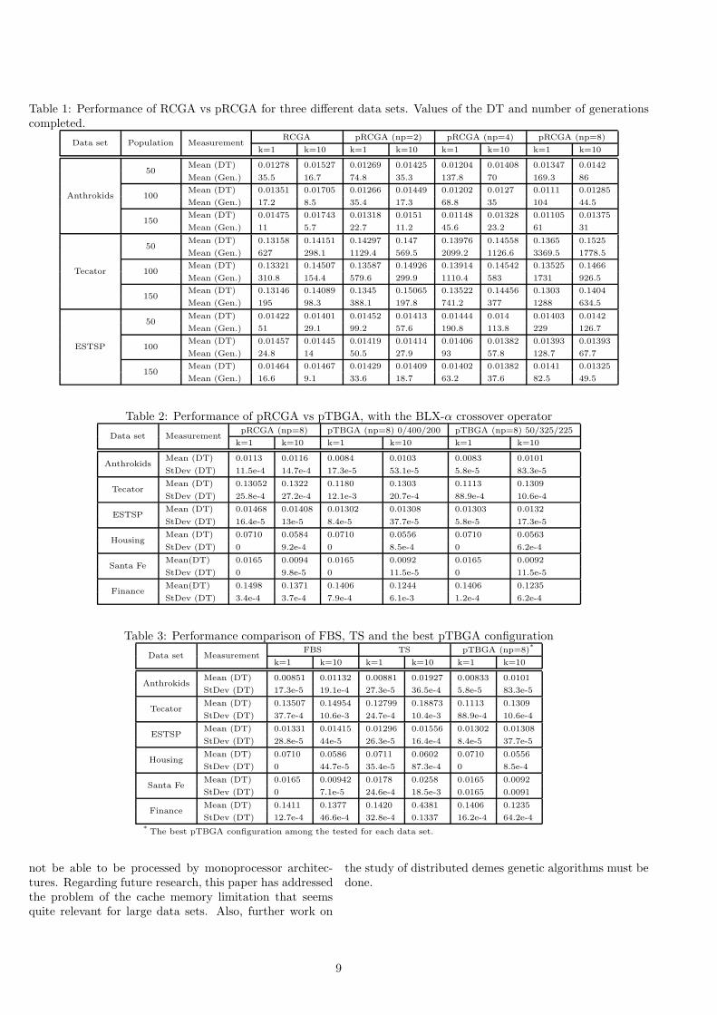
Table 1: Performance of RCGA vs pRCGA for three different data sets. Values of the DT and number of generationscompleted.

Data set Population MeasurementRCGA pRCGA (np=2) pRCGA (np=4) pRCGA (np=8)

k=1 k=10 k=1 k=10 k=1 k=10 k=1 k=10

Anthrokids

50Mean (DT) 0.01278 0.01527 0.01269 0.01425 0.01204 0.01408 0.01347 0.0142

Mean (Gen.) 35.5 16.7 74.8 35.3 137.8 70 169.3 86

100Mean (DT) 0.01351 0.01705 0.01266 0.01449 0.01202 0.0127 0.0111 0.01285

Mean (Gen.) 17.2 8.5 35.4 17.3 68.8 35 104 44.5

150Mean (DT) 0.01475 0.01743 0.01318 0.0151 0.01148 0.01328 0.01105 0.01375

Mean (Gen.) 11 5.7 22.7 11.2 45.6 23.2 61 31

Tecator

50Mean (DT) 0.13158 0.14151 0.14297 0.147 0.13976 0.14558 0.1365 0.1525

Mean (Gen.) 627 298.1 1129.4 569.5 2099.2 1126.6 3369.5 1778.5

100Mean (DT) 0.13321 0.14507 0.13587 0.14926 0.13914 0.14542 0.13525 0.1466

Mean (Gen.) 310.8 154.4 579.6 299.9 1110.4 583 1731 926.5

150Mean (DT) 0.13146 0.14089 0.1345 0.15065 0.13522 0.14456 0.1303 0.1404

Mean (Gen.) 195 98.3 388.1 197.8 741.2 377 1288 634.5

ESTSP

50Mean (DT) 0.01422 0.01401 0.01452 0.01413 0.01444 0.014 0.01403 0.0142

Mean (Gen.) 51 29.1 99.2 57.6 190.8 113.8 229 126.7

100Mean (DT) 0.01457 0.01445 0.01419 0.01414 0.01406 0.01382 0.01393 0.01393

Mean (Gen.) 24.8 14 50.5 27.9 93 57.8 128.7 67.7

150Mean (DT) 0.01464 0.01467 0.01429 0.01409 0.01402 0.01382 0.0141 0.01325

Mean (Gen.) 16.6 9.1 33.6 18.7 63.2 37.6 82.5 49.5

Table 2: Performance of pRCGA vs pTBGA, with the BLX-α crossover operator

Data set MeasurementpRCGA (np=8) pTBGA (np=8) 0/400/200 pTBGA (np=8) 50/325/225

k=1 k=10 k=1 k=10 k=1 k=10

AnthrokidsMean (DT) 0.0113 0.0116 0.0084 0.0103 0.0083 0.0101

StDev (DT) 11.5e-4 14.7e-4 17.3e-5 53.1e-5 5.8e-5 83.3e-5

TecatorMean (DT) 0.13052 0.1322 0.1180 0.1303 0.1113 0.1309

StDev (DT) 25.8e-4 27.2e-4 12.1e-3 20.7e-4 88.9e-4 10.6e-4

ESTSPMean (DT) 0.01468 0.01408 0.01302 0.01308 0.01303 0.0132

StDev (DT) 16.4e-5 13e-5 8.4e-5 37.7e-5 5.8e-5 17.3e-5

HousingMean (DT) 0.0710 0.0584 0.0710 0.0556 0.0710 0.0563

StDev (DT) 0 9.2e-4 0 8.5e-4 0 6.2e-4

Santa FeMean(DT) 0.0165 0.0094 0.0165 0.0092 0.0165 0.0092

StDev (DT) 0 9.8e-5 0 11.5e-5 0 11.5e-5

FinanceMean(DT) 0.1498 0.1371 0.1406 0.1244 0.1406 0.1235

StDev (DT) 3.4e-4 3.7e-4 7.9e-4 6.1e-3 1.2e-4 6.2e-4

Table 3: Performance comparison of FBS, TS and the best pTBGA configuration

Data set MeasurementFBS TS pTBGA (np=8)*

k=1 k=10 k=1 k=10 k=1 k=10

AnthrokidsMean (DT) 0.00851 0.01132 0.00881 0.01927 0.00833 0.0101

StDev (DT) 17.3e-5 19.1e-4 27.3e-5 36.5e-4 5.8e-5 83.3e-5

TecatorMean (DT) 0.13507 0.14954 0.12799 0.18873 0.1113 0.1309

StDev (DT) 37.7e-4 10.6e-3 24.7e-4 10.4e-3 88.9e-4 10.6e-4

ESTSPMean (DT) 0.01331 0.01415 0.01296 0.01556 0.01302 0.01308

StDev (DT) 28.8e-5 44e-5 26.3e-5 16.4e-4 8.4e-5 37.7e-5

HousingMean (DT) 0.0710 0.0586 0.0711 0.0602 0.0710 0.0556

StDev (DT) 0 44.7e-5 35.4e-5 87.3e-4 0 8.5e-4

Santa FeMean (DT) 0.0165 0.00942 0.0178 0.0258 0.0165 0.0092

StDev (DT) 0 7.1e-5 24.6e-4 18.5e-3 0.0165 0.0091

FinanceMean (DT) 0.1411 0.1377 0.1420 0.4381 0.1406 0.1235

StDev (DT) 12.7e-4 46.6e-4 32.8e-4 0.1337 16.2e-4 64.2e-4* The best pTBGA configuration among the tested for each data set.

not be able to be processed by monoprocessor architec-tures. Regarding future research, this paper has addressedthe problem of the cache memory limitation that seemsquite relevant for large data sets. Also, further work on

the study of distributed demes genetic algorithms must bedone.

9

ACKNOWLEDGMENT

This work has been partially supported by the projectsTIN2007-60587, P07-TIC-02768 and P07-TIC-02906, andby research grant BES-2005-9703 from the Spanish Min-istry of Science and Innovation.

REFERENCES

Al-Sultan, K. S. and Al-Fawzan, M. A. (1997). A tabusearch hooke and jeeves algorithm for unconstrained op-timization. European Journal of Operational Research,103(1):198–208.

Alba, E., Luna, F., and Nebro, A. J. (2004). Advances inparallel heterogeneous genetic algorithms for continuousoptimization. Int. J. Appl. Math. Comput. Sci., 14:317–333.

Alba, E. and Tomassini, M. (2002). Parallelism and evolu-tionary algorithms. IEEE Trans. on Evolutionary Com-putation, 6(5):443–462.

Baker, J. E. (1987). Reducing bias and inefficiency in theselection algorithm. In Grefenstette, J. J., editor, Pro-ceedings of the Second International Conference on Ge-netic Algorithms, pages 14–21, Hillsdale, NJ. LawrenceErlbaum Associates.

Brandao, J. (2004). A tabu search algorithm for the openvehicle routing problem. European Journal of Opera-tional Research, 157(3):552–564.

Cantu-Paz, E. (2000). Markov chain of parallel geneticalgorithms. IEEE. Trans. Evolutionary Computation,4:216–226.

Chakraborty, U. K., Deb, K., and Chakraborty, M. (1996).Analysis of selection algorithms: A markov chain ap-proach. Evol. Comput., 4(2):133–167.

De Jong, K. A. (1975). An analysis of the behavior of aclass of genetic adaptive systems. PhD thesis, Universityof Michigan.

De Jong, K. A. (1996). Evolutionary computation: Re-cent developments and open issues. In Goodman, E. D.,Punch, B., and Uskov, V., editors, Proceedings of theFirst International Conference on Evolutionary Compu-tation and Its Applications, pages 7–17, Moscow.

Deb, K. and Goel, T. (2001). Controlled elitist non-dominated sorting genetic algorithms for better con-vergence. In First International Conference on Evo-lutionary Multi-Criterion Optimization, pages 67–81.Springer-Verlag.

DellAmico, M. and Trubian, M. (1993). Applying tabusearch to the job-shop scheduling problem. Ann. Oper.Res., 41(1-4):231–252.

Eirola, E., Liitiainen, E., Lendasse, A., Corona, F., andVerleysen, M. (2008). Using the delta test for variableselection. In ESANN 2008, European Symposium on Ar-tificial Neural Networks, Bruges (Belgium), pages 25–30.

Eshelman, L. and Schaffer, J. (1993). Real-coded geneticalgorithms and interval schemata. In Darrell Whitley,L., editor, Foundation of Genetic Algorithms 2, pages187–202. Morgan-Kauffman Publishers, Inc.

Glover, F. (1986). Future paths for integer programmingand links to artificial intelligence. Comput. Oper. Res.,13(5):533–549.

Glover, F. (1989). Tabu search part i. ORSA Journal onComputing, 1(3):190–206.

Glover, F. (1990). Tabu search part ii. ORSA Journal onComputing, 2:4–32.

Glover, F. (2006). Parametric tabu-search for mixed inte-ger programs. Comput. Oper. Res., 33(9):2449–2494.

Glover, F. and Laguna, F. (1997). Tabu Search. KluwerAcademic Publishers, Norwell, MA, USA.

Goldberg, D. E. (1989). Genetic algorithms in search,optimization and machine learning. Addison Wesley.

Grefenstette, J. J. (1981). Parallel adaptive algorithms forfunction optimization. Technical Report TCGA CS-81-19, Department of Engineering Mechanics, University ofAlabama, Vanderbilt University,.

Guillen, A., Pomares, H., Gonzalez, J., Rojas, I., Herrera,L. J., and Prieto, A. (2008). Parallel multi-objectivememetic rbfnns design and feature selection for functionapproximation problems. In Neurocomputing, In press.

Guillen, A., Rojas, I., Rubio, G., Pomares, H., Herrera,L., and Gonzalez, J. (2008). A new interface for mpi inmatlab and its application over a genetic algorithm. InProceedings of the European Symposium on Time SeriesPrediction, pages 37–46.

Guyon, I., Gunn, S., Nikravesh, M., and Zadeh, A. (2006).Feature extraction: Foundations and applications (Stud-ies in fuzziness and soft computing). Springer-VerlagNew York, Secaucus, NJ, USA.

Hedar, A.-R. and Fukushima, M. (2006). Tabu search di-rected by direct search methods for nonlinear global op-timization. European Journal of Operational Research,170(2):329–349.

Herrera, L., Pomares, H., Rojas, I., Verleysen, M., andGuillen, A. (2006). Effective input variable selection forfunction approximation. Lecture Notes in Computer Sci-ence, 4131:41–50.

Holland, J. J. (1975). Adaption in natural and artificialsystems. University of Michigan Press.

10

Ishibuchi, H., Yoshida, T., and Murata, T. (2003). Balancebetween genetic search and local search in memetic algo-rithms for multiobjective permutation flowshop schedul-ing. IEEE Trans. on Evolutionary Computation, 7:204–223.

Jones, A. (2004). New tools in non-linear modellingand prediction. Computational Management Science,1(2):109–149.

Kosko, B. (1994). Fuzzy systems as universal approxima-tors. Computers, IEEE Transactions on, 43(11):1329–1333.

Lee, S.-W. and Verri, A., editors (2002). Pattern recog-nition with support vector machines, First InternationalWorkshop, SVM 2002, Niagara Falls, Canada, August10, 2002, Proceedings, volume 2388 of Lecture Notes inComputer Science. Springer.

Mantawy, A. H., Soliman, S. A., and El-Hawary, M. E.(2002). A new tabu search algorithm for the long-termhydro scheduling problem. Power Engineering 2002Large Engineering Systems Conference on, LESCOPE02, pages 29–34.

Mateo, F. and Lendasse, A. (2008). A variable selectionapproach based on the delta test for extreme learningmachine models. In Proceedings of the European Sym-posium on Time Series Prediction, pages 57–66.

Michalewicz, Z. (1996). Genetic algorithms + Data struc-tures = Evolution programs. Springer-Verlag, 3rd edi-tion.

Mitchell, M. and Forrest, S. (1995). Genetic algorithmsand artificial life. Artificial Life, 1(3):267–289.

Oh, I.-S., Lee, J.-S., and Moon, B.-R. (2002). Local search-embedded genetic algorithms for feature selection. Pat-tern Recognition, 2002. Proceedings. 16th InternationalConference on, 2:148–151 vol.2.

Oh, I.-S., Lee, J.-S., and Moon, B.-R. (2004). Hy-brid genetic algorithms for feature selection. IEEETrans. on Pattern Analysis and Machine Intelligence,26(11):1424–1437.

Pi, H. and Peterson, C. (1994). Finding the embedding di-mension and variable dependencies in time series. NeuralComputation, 6(3):509–520.

Poggio, T. and Girosi, F. (1989). A theory of networks forapproximation and learning. Technical Report AI-1140,MIT Artificial Intelligence Laboratory, Cambridge, MA.

Punch, W. F., Goodman, E. D., Pei, M., Chia-Shun, L.,Hovland, P., and Enbody, R. (1993). Further researchon feature selection and classification using genetic al-gorithms. In Forrest, S., editor, Proc. of the Fifth Int.Conf. on Genetic Algorithms, pages 557–564, San Ma-teo, CA. Morgan Kaufmann.

Rasmussen, C. E. (2004). Gaussian processes in machinelearning, volume 3176 of Lecture Notes in Computer Sci-ence, pages 63–71. Springer-Verlag, Heidelberg. Copy-right by Springer.

Raymer, M., Punch, W., Goodman, E., Kuhn, L., andJain, A. (2000). Dimensionality reduction using geneticalgorithms. Evolutionary Computation, IEEE Transac-tions on, 4(2):164–171.

Reeves, C. R. (1993). Using genetic algorithms with smallpopulations. In Forrest, S., editor, Proceedings of theFifth International Conference on Genetic Algorithms,pages 92–99. Morgan Kaufmann.

Rosenblatt, F. (1958). The perceptron: A probabilisticmodel for information storage and organization in thebrain. Psychological Review, 65:386–408.

Saeys, Y., Inza, I., and Larranaga, P. (2007). A review offeature selection techniques in bioinformatics. Bioinfor-matics, 23(19):2507–2517.

Scheuerer, S. (2006). A tabu search heuristic for thetruck and trailer routing problem. Comput. Oper. Res.,33(4):894–909.

Sywerda, G. (1989). Uniform crossover in genetic algo-rithms. In Proceedings of the third international confer-ence on Genetic algorithms, pages 2–9, San Francisco,CA, USA. Morgan Kaufmann Publishers Inc.

Wang, L. and Kazmierski, T. (2005). Vhdl-ams based ge-netic optimization of a fuzzy logic controller for auto-motive active suspension systems. Behavioral Modelingand Simulation Workshop, 2005. BMAS 2005. Proceed-ings of the 2005 IEEE International, pages 124–127.

Xu, J., Chiu, S., and Glover, F. (1996a). A probabilistictabu search for the telecommunications network design.Journal of Combinatorial Optimization, Special Issue onTopological Network Design, 1:69–94.

Xu, J., Chiu, S., and Glover, F. (1996b). Using tabu searchto solve steiner tree-star problem in telecommunicationsnetwork design. Telecommunication Systems, 6:117–125.

Zhang, C., Li, P., Guan, Z., and Y. Rao, Y. (2007). Atabu search algorithm with a new neighborhood struc-ture for the job shop scheduling problem. Computers &Operations Research, 34(11):3229–3242.

Zhang, J., Li, S., and Shen, S. (2006). Extracting minimumunsatisfiable cores with a greedy genetic algorithm. InProc. ACAI06, pages 847–856.

11

���

���

���

���

���

Gen

era

tio

ns

Anthrokids (k=1)

�

��

��

��

��

� � � � � � �

Gen

era

tio

ns

Number of processors

Population=50 Population=100 Population=150

Figure 2: Generations evaluated by the GA vs the numberof processors used. Anthrokids without scaling.

����

����

����

����

����

Gen

era

tio

ns

Tecator (k=1)

�

���

����

����

����

� � � � � � �

Gen

era

tio

ns

Number of processors

Population=50 Population=100 Population=150

Figure 3: Generations evaluated by the GA vs the numberof processors used. Tecator without scaling.

���

���

���

���

Gen

era

tio

ns

ESTSP (k=1)

�

��

��

���

� � � � � � �

Gen

era

tio

ns

Number of processors

Population=50 Population=100 Population=150

Figure 4: Generations evaluated by the GA vs the numberof processors used. ESTSP without scaling.

��

��

��

��

��

���

Gen

era

tio

ns

Anthrokids (k=10)

�

��

��

�

�

��

� � � � � �

Gen

era

tio

ns

Number of processors

Population=50 Population=100 Population=150

Figure 5: Generations evaluated by the GA vs the numberof processors used. Anthrokids with scaling.

����

����

����

����

����

����

Gen

era

tio

ns

Tecator (k=10)

�

���

���

���

���

����

� � � � � � �

Gen

era

tio

ns

Number of processors

Population=50 Population=100 Population=150

Figure 6: Generations evaluated by the GA vs the numberof processors used. Tecator with scaling.

��

���

���

���

Gen

era

tio

ns

ESTSP (k=10)

�

��

��

��

� � � � � � �

Gen

era

tio

ns

Number of processors

Population=50 Population=100 Population=150

Figure 7: Generations evaluated by the GA vs the numberof processors used. ESTSP with scaling.

12