On-line production cost optimization in high

performance machining operations for mould and die

manufacturing

‡Jorge A. Silva A., †José Vicente Abellán-Nebot,

‡Hector R. Siller, ‡Federico Guedea Elizalde

‡ Center for Innovation in Design and Technology, Tecnológico de Monterrey,

Monterrey, México.

Address: Av. Eugenio Garza Sada #2501 Sur, 64849.

Tel.: +52 (81) 8358 2000 ext. 5149

† Dept. of Industrial Systems Engineering and Design, Universitat Jaume I.

Castellón, Spain.

Address: Av. Sos Baynat s/n, 12071.

Tel.:+34-964-728186, Fax:+34-964-728170.

* Corresponding author: hector.siller@itesm.mx

On-line production cost optimization in high

performance machining operations for mould and die

manufacturing

Abstract— This paper proposes an on-line adaptive

control with optimization (ACO) methodology for

optimizing the production cost subjected to quality

constraints in high performance machining operations

of hardened steel (58-62HRC). Unlike traditional

approaches for optimizing production cost, this paper

deals with optimizing the cutting operation

considering the current state of the cutting-tool.

Artificial intelligence techniques for modeling

(Artificial Neural Networks) and optimizing (Genetic

Algorithms and Mesh Adaptive Direct Search algorithms)

are applied for this purpose. As a result, the

production cost estimation from the proposed approach

is 13% lower than the one obtained by the traditional

approach with 76% less uncertainty.

Keywords: Artificial Neural Networks; machining cost;

Adaptive Control with Optimization (ACO); Genetic

Algorithms; Mesh Adaptive Direct Search algorithms;

high performance machining.

1. Introduction

The machining of hardened steels (58-62HRC) for moulds and

dies requires costly and time-consuming operations such as

electrical discharge machining (EDM) and grinding

operations in order to meet part quality specifications.

Recently, the emerging field of hard cutting to avoid these

inefficient operations is gaining popularity. In hard

cutting, high-performance machining centres with special

cutting-tools such as Cubic Boron Nitride (CBN) tools are

used to meet quality specifications without conducting

subsequent grinding operations. In this field, first

introductory steps have been made in automotive, gear,

bearing, tool and die making industry (Tönshoff 2000).

Cutting parameter selection for minimizing production

cost in hard cutting operations requires the evaluation of

cutting-tool costs and non-quality costs. Current practices

(traditional approach) for selecting optimal cutting

parameters are based on minimizing the production cost

assuming that the estimation of cutting-tool life and

surface roughness from empirical well-known models are

reliable. Furthermore, the surface roughness is commonly

assumed independent from the cutting-tool wear so the

cutting parameters selection is done off-line. However, for

hard cutting operations these assumptions may be not true

(Siller 2008).

In (Benardos 2002) some examples in which the

increased cutting-tool wear may influence the surface

roughness are stated. First, the cutting edge

irregularities will leave visible traces on the surface

during machining. Second, cutting-tool wear is able to

produce vibrations and to alter cutting conditions and

forces, which does not favour good surface roughness.

Considering that face milling is a multi-point cutting

process, the problem becomes even more complicated. In (Dae

Kyun Baek 1997), it is suggested that both static (cutting

speed, feed, depth of cut) and dynamic variables (dynamic

behaviour of the cutting tool-workpiece system through the

measurement of cutting forces) of the milling process

should be included in the surface roughness model. (Figure

1.1) shows a set of factors that can affect the surface

roughness.

[Insert Figure 1.1 about here]

In the literature, the adaptation of cutting

parameters according to the state of the machining

operation has been successfully implemented. Three major

strategies are identified:

Adaptive Control with Constraints (ACC),

Geometric Adaptive Control (GAC).

Adaptive Control with Optimization (ACO)

In the ACC systems, process parameters are manipulated

in real time to maintain a specific process variable, such

as force or power, at a constraint value (Zuperl 2005). In

the GAC systems, process parameters are modified to

maintain product quality such as dimensional accuracy

and/or surface finish (Coker 1996). In ACO systems the

controller adjusts the operating parameters to maximize a

given performance index under various constraints whereas

in ACC systems the operating parameters are adjusted to

regulate one or more output parameters to their limit

values (Liang 2004). Traditionally, ACO systems have dealt

with adjusting cutting parameters (feed rate, spindle speed

and depth of cut) to maximize material removal rate subject

to constraints such as surface roughness, power

consumption, cutting forces, etc (Gopal 2003). In (Billatos

1991) an ACO system was researched to determine the optimum

feed rate and spindle speed in order to maximize the

material removal rate. In (Ulsoy 1989) an ACO system for

maximizing an economic index on-line was developed, based

on the measurement of cutting forces (Yanming Liu 1999)

(Zuperl 2011), cutting torque, tool temperature and the

machine tool thermal errors (Yang 2005). However, none of

these strategies have been implemented for adapting cutting

parameters to minimize production cost updating it

according to the current state of the cutting operation.

In this paper an ACO method for product cost

optimization of hard cutting operations is presented. The

proposed system adjusts cutting parameters during the

cutting-tool life cycle every time a tool pass is over in

order to minimize on-line the cutting tool pass cost.

2. Traditional cutting parameters optimization

The traditional machining economics problem consists in

determining the optimal cutting parameters in order to

maximize or minimize an objective function based on a

desired economic criterion and subjected to the constraints

applicable to the machining system. Three economic criteria

are commonly applied: production time, production cost and

profit rate. The maximum production objective (minimum

production time) seeks to identify the cutting conditions

that best balance the material removal rate (MRR) and tool

life to produce the highest output. The production cost

objective seeks to find a balance between MRR and tool life

to produce at the lowest cost. For the case of the maximum

rate of profit criteria, there is a balance between the

contributions of both minimum production cost and

production time criteria into the objective function. For

practical purposes it has been found that unless the profit

margin is very high, the optimum conditions predicted by

the maximum profit rate criterion tends to lie close to the

minimum production cost (Stephenson 1997). In this paper,

without loss of generality, the economic criterion analyzed

is the minimum production cost.

2.1. Production Cost

In machining systems, the time to produce a part lot (Tu)

can be defined by Equation (1):

(1)

Where

ts is the set up time,

tm the machining time,

ttc the tool change time and

T the expected cutting tool life.

For milling operations, the machining time is defined by

Equation (2) (Stephenson 1997):

(2)

where D is the rotary cutting-tool diameter, L the

workpiece length to be machined, Vc the cutting speed, fz

the feed per tooth, np the number of parts to be machined,

z the number of teeth, ε the over-travel of the milling

cutter on the workpiece, e the thickness of the workpiece

to be machined, and ap the axial depth of cut. Denoting Dt

as the workpiece diameter and fr as the feed per

revolution, the machining time equation for turning

operations is defined as Equation (3):

(3)

The production cost for a part lot (Cu) can be

formulated as Equation (4):

(4)

where cmat is the cost of the raw material per part, c1 is

the labour cost, c0 is the overhead cost and ct is the cost

of the cutting tool.

Additionally, in hard cutting operations the cost of

quality loss due to the deviation of the part surface

quality (measured as the surface roughness -Ra-) from its

desired value should be considered. For this purpose, the

Taguchi’s loss quality function can be added as an

additional cost. This quality loss cost is formulated as

Equation (5) (M.H. 2000):

(5)

where β2 is the mean square deviation of Ra and Δ2 is the

maximum admissible square deviation of Ra from

specifications, which are expressed respectively as

Equation (6) and Equation (7):

(6)

(7)

From previous equations, Ramax is the maximum Ra

defined by the specifications; Ratgt is the desired Ra; Raavg

is the expected Ra of the machined workpiece; and Arw is

the part cost if the part is outside of specifications.

Therefore, the minimum production cost will be

obtained by optimizing the following equation:

(8)

Ctot being the total cost, Cu the production cost and Cq the

quality loss cost.

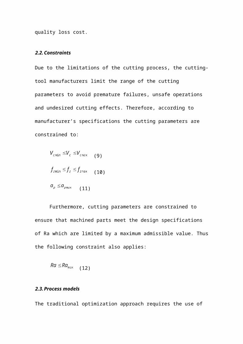
2.2. Constraints

Due to the limitations of the cutting process, the cutting-

tool manufacturers limit the range of the cutting

parameters to avoid premature failures, unsafe operations

and undesired cutting effects. Therefore, according to

manufacturer’s specifications the cutting parameters are

constrained to:

(9)

(10)

(11)

Furthermore, cutting parameters are constrained to

ensure that machined parts meet the design specifications

of Ra which are limited by a maximum admissible value. Thus

the following constraint also applies:

(12)

2.3. Process models

The traditional optimization approach requires the use of

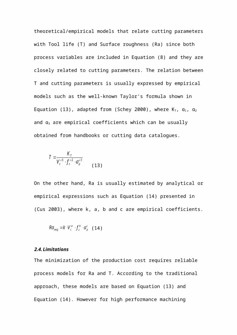
theoretical/empirical models that relate cutting parameters

with Tool life (T) and Surface roughness (Ra) since both

process variables are included in Equation (8) and they are

closely related to cutting parameters. The relation between

T and cutting parameters is usually expressed by empirical

models such as the well-known Taylor‘s formula shown in

Equation (13), adapted from (Schey 2000), where KT, α1, α2

and α3 are empirical coefficients which can be usually

obtained from handbooks or cutting data catalogues.

(13)

On the other hand, Ra is usually estimated by analytical or

empirical expressions such as Equation (14) presented in

(Cus 2003), where k, a, b and c are empirical coefficients.

(14)

2.4. Limitations

The minimization of the production cost requires reliable

process models for Ra and T. According to the traditional

approach, these models are based on Equation (13) and

Equation (14). However for high performance machining

operations these models tend to generate inaccurate

estimations. Firstly, the use of Taylor’s equation for

estimation of tool life in cutting tool materials such as

CBN tools may not provide accurate estimations as reported

in (Trent 2000). Secondly, surface roughness generation is

influenced by additional mechanisms such as vibrations,

engagement of the cutting tool, built up edge and tool wear

among others, especially in high performance machining

operations (Siller 2008). So Equation (14) may be

inadequate to model Ra.

Additionally, even if these models were accurate

enough, the traditional optimization methods cannot

consider the current state of the cutting tool during the

operation since this optimization procedure fixes the

cutting parameters for the whole cutting tool life. It

seems that a more efficient approach would result if the

cutting conditions can be modified according to the current

state of the cutting tool and the actual surface roughness

values.

3. Proposed adaptive control optimization system

The proposed Adaptive Control Optimization (ACO) system

overcomes the limitations of traditional optimization

approaches using in-process sensor measurements as well as

robust and reliable artificial intelligent (AI) process

models.

The proposed ACO system is described in (Figure 3.1)

and its operation is described as follows. After each

cutting-tool pass, the ACO system obtains information of

the operation by sensors installed in the machine-tool.

After conditioning the signals and extracting their

descriptors (significant values such as average, root mean

square -RMS-, etc.), these values are used by the process

models to estimate the current performance of the machining

(current tool wear -Tw-, Ra, etc.). The process models are

based on AI techniques and were previously learnt from

experimental data. Using the estimations from the AI

models, the objective function is optimized by a

combination of optimization techniques for black box models

such as genetic algorithms (GA) and mesh adaptive direct

search (MADS) algorithms (Shan 2010). The optimization

provides the optimal cutting parameters for the next

cutting-tool pass, which are sent to the numerical control

system of the machine-tool.

[Insert Figure 3.1 about here]

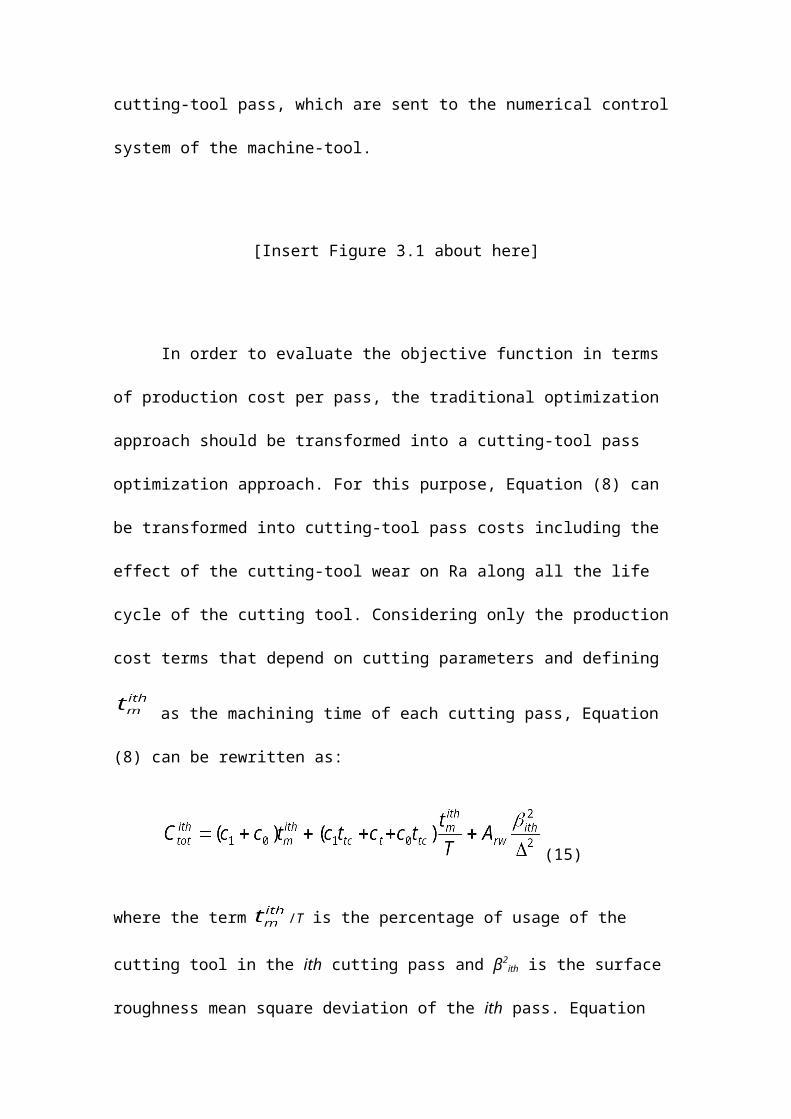
In order to evaluate the objective function in terms

of production cost per pass, the traditional optimization

approach should be transformed into a cutting-tool pass

optimization approach. For this purpose, Equation (8) can

be transformed into cutting-tool pass costs including the

effect of the cutting-tool wear on Ra along all the life

cycle of the cutting tool. Considering only the production

cost terms that depend on cutting parameters and defining

as the machining time of each cutting pass, Equation

(8) can be rewritten as:

(15)

where the term /T is the percentage of usage of the

cutting tool in the ith cutting pass and β2ith is the surface

roughness mean square deviation of the ith pass. Equation

(15) is the objective function to be minimized every

cutting-tool pass in the ACO system.

3.1. Selection of AI technique for process modelling

A machining process is non-linear and time-dependant;

therefore it’s difficult to provide an accurate model

utilizing a traditional identification method. For this

reason, the introduction of new techniques such as the ones

based in artificial intelligence has had a great impact in

this field. Artificial Neural Networks (ANN) have received

considerable and increasing interest over the past decade.

Compared to the traditional computing methods, an ANN is

robust and global. It can be used to learn any non-linear

function and can be used for any non-linear optimization

problem. ANNs are widely used for system modelling, machine

learning, function optimizing, image processing and

intelligent control. In the field of part quality

prediction in machining systems, ANNs represent almost the

60% of AI approaches applied in the literature (Abellan-

Nebot 2010) (Abellan-Nebot & Romero 2010). Research works

in Refs. (Liu 1999), (Azlan 2010) and (Aguilar 2006) show

some previous works that have successfully applied ANN to

model and predict Ra in milling and turning operations.

ANNs give a kind of implicit relationship between the

inputs and outputs by learning from a data set that

represents the behaviour of a system (El-Mounayri 2005). In

(Briceno 2002) two commonly used ANN structures are

compared for measuring their accuracy and efficiency in

modelling a milling system, one of them being a Back

Propagation (BP) ANN using the Levenberg-Marquardt

algorithm with one hidden layer (given White’s theorem

which states that “one layer with non-linear activation

functions is sufficient to map any non-linear functional

relationship with a reasonable level of accuracy”) and a

minimum of two neurons in the hidden layer. The study

concludes that the BP ANN with the mentioned configuration

can be trained to model the system using a full factorial

design of experiments and offer a good generalization

methodology and a fast convergence.

4. Experimental case study

4.1. Experimental setup

A manufacturing process of moulds for the tile industry was

analyzed to implement the ACO system proposed in this

paper. The workpiece material are squared plates of AISI D3

steel (250 x 250 mm; 60 HRC) and the cutting-tool used is a

CBN round insert with an effective cutting diameter of 40

mm. For manufacturing a part, eight face milling cutting-

tool passes are conducted under a vertical machining centre

suited for mould components manufacturing. The fixed

cutting conditions, part specifications and cost constants

are shown in (Table 4.1).

Table 4.1 Constants.

Cutting Conditions Cost Constants

Radial depthof cut

ae

31.25

mmTool Cost Ct 90€

Axial Depthof Cut

ap 0.4 mm Overhead Cost C0

10

€/hr

Part Specifications Labor Cost C1

40

€/hr

SurfaceRoughness

Ra <0.2 µmPiece Rework

CostArw 75 €

Tool Constants Lot Size np50 pcs

Tool ChangeTime

ttc 10 sec

For this application, the cutting parameters Vc and fz

have to be selected for minimum production cost. In order

to model the process variables, a full factorial design of

experiments (DoE) was conducted. Three levels per each

factor were considered to acquire lineal and quadratic

effects. The factor combinations used are shown in (Table

4.2). For each experiment the face milling operation was

carried out until the cutting tool edge was worn (VB > 0.3

mm, usual value for face milling finishing operations

according to ISO standards (ISO 1989)) or the Ra was out of

specifications. For each cutting-tool pass, detailed

measurements of surface roughness and machining forces were

obtained. Ra was measured using a Mitutoyo ™ Surftest 301

profilometer using a sampling length λ = 0.8 mm and a

number of spans n = 5. Cutting forces were acquired from a

piezoelectric dynamometer installed on the machine-tool

table and the descriptor analyzed was the RMS value of the

cutting force. After the experimentation, a data-set of 160

samples was obtained due to the tool wear reaching its

limit value for each combination of cutting conditions. The

full data on Ra is shown in (Table 4.3).

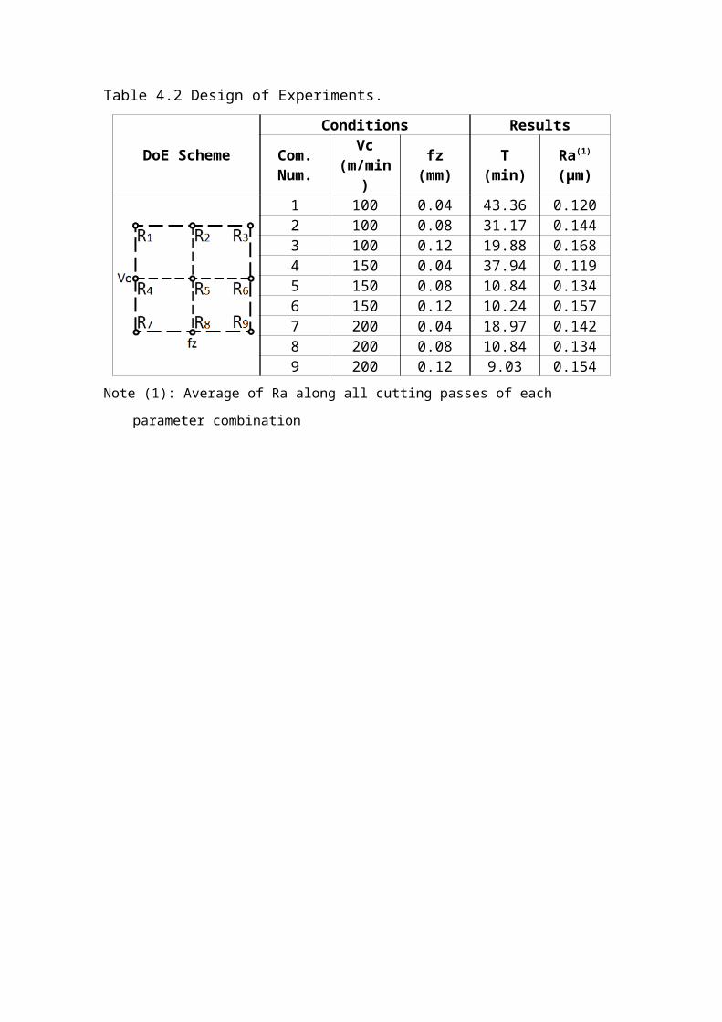
Table 4.2 Design of Experiments.

DoE Scheme

Conditions Results

Com.Num.

Vc(m/min

)

fz (mm)

T (min)

Ra(1)

(μm)

1 100 0.04 43.36 0.1202 100 0.08 31.17 0.1443 100 0.12 19.88 0.1684 150 0.04 37.94 0.1195 150 0.08 10.84 0.1346 150 0.12 10.24 0.1577 200 0.04 18.97 0.1428 200 0.08 10.84 0.1349 200 0.12 9.03 0.154

Note (1): Average of Ra along all cutting passes of each

parameter combination

Table 4.3 Ra [µm] results of training samples.Pass

Condition 1 2 3 4 5 6 7 8 9 10 11 12

1 0.10

0.08

0.09

0.09

0.12

0.14

0.13

0.13

0.11

0.1

0.13

0.12

2 0.11

0.11

0.11

0.11

0.11

0.13

0.14

0.13

0.11

0.12

0.15

0.14

3 0.13

0.14

0.13

0.12

0.13

0.15

0.15

0.16

0.16

0.18

0.15

0.18

4 0.09

0.11

0.11

0.11

0.12

0.13

0.11

0.12

0.14

0.11

0.12

0.10

5 0.11

0.12

0.11

0.12

0.18

0.14

0.14

0.15

0.14

0.14

0.14

0.12

6 0.14

0.14

0.15

0.14

0.16

0.15

0.18

0.15

0.15

0.15

0.16

0.16

7 0.15

0.12

0.11

0.13

0.13

0.15

0.17

0.16

0.13

0.15

0.14

0.15

8 0.11

0.11

0.14

0.11

0.13

0.12

0.14

0.15

0.13

0.12

0.14

0.15

9 0.11

0.13

0.15

0.17

0.17

0.17

0.17

0.17

0.15

0.14

0.13

0.14

PassCondition 13 14 15 16 17 18 19 20 21 22 23

1 0.16

0.15

0.15

0.14

2 0.16

0.17

0.17

0.18

0.17

0.17

0.17

0.17

0.16

0.17

0.18

3 0.19

0.18

0.21

0.21

0.18

0.20

0.20

0.21

0.19

0.20

4 0.13

0.13

0.13

0.13

0.12

0.12

0.12

0.12

0.14

5

6 0.18

0.17

0.17

0.18

7 0.13

0.18

8 0.14

0.14

0.16

0.16

9 0.15

0.15

0.16

0.17

0.15

0.15

0.17

0.20

4.2. Traditional optimization results

In order to conduct the traditional optimization procedure,

the process models of T and Ra, defined by Equation (13)

and Equation (14) respectively, were fitted from

experimental data. The T model was fitted with a

coefficient of determination of R2 = 90% and a standard

deviation of the error between the model and the

experimental results σT = 0.2 min; and the Ra model was

fitted with R2 = 67.4% and σRa = 0.0221 µm. (Table 4.4) and

(Table 4.5) show the results of the analysis of variances

for both models. The Ra model was not very accurate as

indicated by the low value of R2 which is an important

limitation for the reliability of the production cost

estimation.

Table 4.4. Analysis of variances for Tool-life (T).

SourceDegrees

offreedom

Sum ofSquare

s

Mean ofthe Sum

ofSquares

F P-value

Regression 2 0.5034

7 0.25173 26.94 0.001

Residual Error 6 0.0560

6 0.00934

Total 8 0.55953 R2=90%

Table 4.5. Analysis of variances for surface roughness

(Ra).

SourceDegrees

offreedom

Sum ofSquare

s

Mean ofthe Sum

ofSquares

F P-value

Regression 2 0.0141

37 0.007068 6.21 0.035

Residual Error 6 0.0068

32 0.001139

Total 8 0.020969

R2=67.4%

The resulting process models of T and Ra are:

(16)

(17)

For the traditional method, the optimization of Equation

(15) is conducted through any conventional optimization

technique. The resulting optimal parameters were Vc = 200

m/min and fz = 0.089 mm/tooth, which determines a

production cost per part of 79.1 €. (Figure 4.1) shows the

resulting model and the location of the optimal point.

[Insert Figure 4.1 about here]

4.3. Proposed ACO system optimization results

The ACO system implemented is composed of three process

models: a cutting-tool wear model for diagnosing the state

of the cutting tool (percentage of effective cutting

machining life time); a surface roughness model for

predicting the Taguchi’s quality loss; and a cutting tool-

life model. All models were developed using Back-

Propagation Artificial Neural Networks (BP ANN) to model

the non-linear relationships in machining processes. The

characteristics of the ANN models are described in (Table

4.6).

Table 4.6. ANN Models description

ANN Models

Cutting ToolWear Model

SurfaceRoughness

Model

Tool LifeModel

Type Backpropagation

Backpropagat

ion

Backpropagat

ion

Inputs Vc, fz, , Fc

(RMS)

Vc, fz,TB

Vc, fz

Outputs Tw Ra THiddenLayers 1 1 1

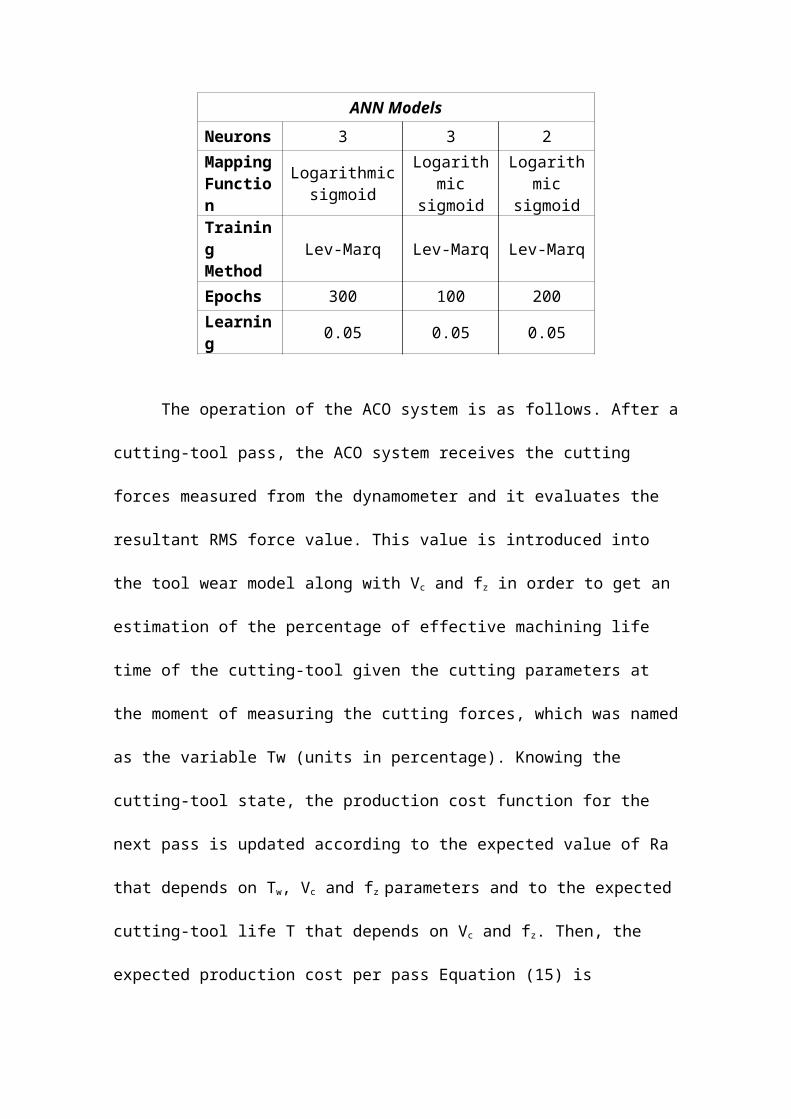
ANN ModelsNeurons 3 3 2MappingFunction

Logarithmicsigmoid

Logarithmic

sigmoid

Logarithmic

sigmoidTraining Method

Lev-Marq Lev-Marq Lev-Marq

Epochs 300 100 200Learning 0.05 0.05 0.05

The operation of the ACO system is as follows. After a

cutting-tool pass, the ACO system receives the cutting

forces measured from the dynamometer and it evaluates the

resultant RMS force value. This value is introduced into

the tool wear model along with Vc and fz in order to get an

estimation of the percentage of effective machining life

time of the cutting-tool given the cutting parameters at

the moment of measuring the cutting forces, which was named

as the variable Tw (units in percentage). Knowing the

cutting-tool state, the production cost function for the

next pass is updated according to the expected value of Ra

that depends on Tw, Vc and fz parameters and to the expected

cutting-tool life T that depends on Vc and fz. Then, the

expected production cost per pass Equation (15) is

optimized applying sequentially a Genetic Algorithm (GA)

and a Mesh Adaptive Direct Search (MADS) algorithm.

Basically, the GA is firstly applied to find the general

region where the objective function is a minimum. Then, the

MADS refines the search using the GA solution as the

starting point of the mesh. The optimization results are

the optimal parameters for the next machining pass (Vc and

fz), as well as the expected values for Ra and Ctotith. The

procedure is repeated until the cutting-tool wear (Tw) is

estimated by the model to be higher than 95% of the tool

lifetime, when a cutting-tool replacement is conducted. The

characteristics of the GA and MADS algorithm are shown in

(Tables 4.7) and (Table 4.8) respectively, followed by the

flowchart for both algorithms in (Figure 4.2) and

(Figure4.3).

Table 4.7. Optimization algorithms description

Genetic AlgorithmVariables to optimize

Vc, fz

Elite count 2

Population size 10 Mutation funct. Gaussian

Stall generations 7 Selection

funct. Stochastic

Stall time 6 sec Generations 15

Crossover frac. 0.8 Initial Vc=[100, 200]

Genetic Algorithmranges fz=[0.04, 0.12]

[Insert Figure 4.2 about here]

Table 4.8. Optimization algorithms description

Mesh Adaptive Direct SearchVariables to optimize

Vc, fz

Contraction 2

Initial mesh size 0.05 Poll method Positive basis

2N

Max. mesh size Inf Polling order Consecutive

Min. mesh size Inf Stop criterion

Tolerance mesh: 5x10-4

ExpansionFactor 2

[Insert Figure 4.3 about here]

The error standard deviation of the models for T and

Ra were found to be σT = 0.006 min and σRa = 0.0155 µm. An

example of the optimization results from the ACO system is

shown in (Figure 4.4) and (Figure 4.5). (Figure 4.4) shows

the production cost per pass when Tw = 24% of the tool life

time, with optimal parameters Vc = 116 m/min and fz = 0.087

mm/tooth; (Figure 4.5) shows the production cost per pass

for a Tw =84%, where the optimal parameters Vc = 195 m/min

and fz = 0.115 mm/tooth.

[Insert Figure 4.4 about here]

[Insert Figure 4.5 about here]

4.4. Experimental validation results

For validation purposes two plates were machined: one using

the parameters obtained from the ACO system and a second

one using the parameters from the traditional approach.

(Figure 4.6) shows the comparison of the production cost

per pass obtained for each case and (Figure 4.7) shows the

surface roughness expected results from the optimization

procedures (simulated) and the actual results after

machining (experimental).

For the first plate, the proposed optimization

approach resulted in an expected production cost of 61.41

€; and experimentally the production cost was 64.17 €. For

the second plate, the traditional approach resulted in an

expected production cost of 79.15 €, and experimentally the

production cost was 73.46 €. Therefore, the proposed

optimization approach reduces the cost in a 12.64 %

experimentally. It is worth mentioning that the Ra was also

well contained within the limits of its specification (Ra <

0.2 µm) at all times (see Figure 4.6).

[Insert Figure 4.6 about here]

[Insert Figure 4.7 about here]

4.5. Uncertainty of Production Cost Estimation

It should be noted that the cost estimation is subjected to

an uncertainty since models are not perfect. In order to

estimate the range in which the real cost of the production

will lie due to the models’ uncertainty, the derivative of

Equation (15) should be analyzed. Equation (18) shows the

derivative of Equation (15) with respect to T and Ra. The

values for dT and dRa represent the error of the estimation

of T and Ra and are calculated as ±2σ, for a 95 %

confidence of the resulting value being in this range,

obtained from the standard deviation of the error of the T

and Ra models.

(18)

(19)

(20)

Evaluating Equation (20) using the traditional and the

proposed approach, the uncertainties of the production cost

estimation per part are ±44.32 € and ±10.76 € respectively.

Therefore, the uncertainty of the cost estimation is

greatly reduced (75.7 %) which is mainly explained by the

better performance of ANN models to estimate the machining

process variables.

5. Conclusion and future work

An ACO system based on AI techniques and a dynamometer for

minimizing production cost every cutting-tool pass

considering the effect of tool wear on surface roughness

was presented in this paper. Unlike traditional

optimization techniques, this methodology allows the system

to adapt the cutting parameters according to the cutting-

tool state. The proposed ACO system was experimentally

compared with the traditional optimization procedure on a

high performance machining process with CBN tools.

The expected optimal cutting conditions by the

traditional approach were Vc = 200 m/min and fz = 0.089 mm

with a total production cost per part of 73.46 €. On the

other hand, the proposed ACO system decreases the final

production cost per part to 64.17 € by adapting the cutting

conditions each cutting pass, which means a decrease of

12.64 % in the production cost. Furthermore, the

uncertainty of the production cost estimation was 75.7 %

lower with the proposed approach than with the traditional

one. The better performance of the proposed approach was

mainly due to two reasons. First, the ANN process models

showed a more accurate estimation than empirical regression

models so the optimal parameters are closer to the reality.

Secondly, the on-line nature of the ACO system allows

adapting the cutting parameters every cutting pass so the

system is more flexible to adapt to any change in the

objective function during the cutting-tool life-cycle,

minimizing the total production cost per part considerably.

As future work, the authors suggest to investigate the

implementation of ACO systems based on other non-intrusive

sensor systems such as current sensors or accelerometers.

The use of the presented ACO system based on dynamometer

has limited industrial applicability due to the intrusive

nature on the process. Furthermore, for the case study

analyzed, the high impact of workpiece hardness on surface

roughness should be investigated in more detail to ensure a

real optimal production cost.

6. Acknowledgment

The authors would like to express their gratitude to the

Department of Engineering Systems and Design of the

Universitat Jaume I, to the Intelligent Machines Research

Group at Tecnológico de Monterrey, to CONACYT exchange

scholarship program for its support, and to Miguel Aymerich

for his help in gathering the experimental data.

References

Abellan-Nebot, J.V, 2010. A review of artificial

intelligent approaches applied to part accuracy prediction,

Int. J. Machining and Machinability of Materials, Vol. 8, Nos. 1/2,

pp.6–37.

Abellan-Nebot, J.V. and Romero, F., 2010. A review of

machining monitoring systems based on artificial

intelligence process models. Int. Journal Advanced Manufacturing

Technology, Vol. 47, Nos. 1-4, pp.237–257.

Aguilar Martinez, Sheyla Yael, 2006. Surface roughness modeling

in machining pocesses. MS thesis. ITESM, Monterrey.

Azlan Mohd Zain, Habibollah Haron and Safian Sharif, 2010.

Prediction of surface roughness in the end milling

machining using Artificial Neural Network. Expert Systems with

Applications, 37: 1755-1768.

Benardos, P.G. and Vosniakos, G.C., 2002. Prediction of

surface roughness in CNC face milling using neural networks

and Taguchi’s design of experiments. Robotics and Computer

Integrated Manufacturing, 18:343-354.

Benardos, P.G. and Vosniakos, G.C., 2003. Predicting

surface roughness in machining: A review. International Journal

of Machine Tools & Manufacture, 43: 833-844.

Billatos, S.B. and Tseng, P.C., 1991. Knowledge-based

optimization for intelligent machining. Journal of Manufacturing

Systems. 10(6):464-475.

Briceno, Jorge F., El-Mounayri, H. and Mukhopadhyay, S.,

2002. Selecting an artificial neural network for efficient

modeling and accurate simulation of the milling process.

International Journal of Machine Tools & Manufacture, 42:663–674.

Coker, S.A. and Shin, Y.C., 1996. In-process control of

surface roughness due to tool wear using a new ultrasonic

system. International Journal of Machine Tools and Manufacture, 36(3):

411-422.

Cus, F. and Balic, J., 2003. Optimization of cutting

process by GA approach. Robotics and Computer-Integrated

Manufacturing, 19(1):189-199.

Dae Kyun Baek, Tae Jo Ko and Hee Sool Kim, 1997. A dynamic

surface roughness model for face milling. Precision Engineering,

20(3):171-178.

El-Mounayri, H., Kishawy, H. and J. Briceno, 2005.

Optimization of CNC ball end milling: a neural network-

based model. Journal of Materials Processing Technology, 166: 50–62.

Gopal, A.V. and Rao, P.V., 2003. Selection of optimum

conditions for maximum material removal rate with surface

finish and damage as constraints in sic grinding.

International Journal of Machine Tools and Manufacture, 43(13):1327-

1336.

ISO. Tool life test in milling, part 1: Face milling.

International standard Organization (ISO), 1989.

Koren, Y., 1983. Adaptive Control Systems. Computer Control of

Manufacturing Systems. New York: Macgraw-hill. Page: 193-219.

Liang, S.Y., Hecker, R.L. and Landers, R.G., 2004.

Machining Process monitoring and Control: The State-of-the-

Art. Journal of Manufacturing Science and Engineering- Transactions of the

ASME, 126(2):297-310.

Liu, Y.M. and Wang, C.J., 1999. Neural network based

adaptive control and optimization in the milling process.

International Journal of Advanced Manufacturing Technology, 15(11):791-

795.

M.H., and Li, C., 2000. Quality loss function based

manufacturing process setting models for unbalanced

tolerance design. International Journal of Advanced Manufacturing

Technology. 16:39–45.

Schey, J.A. Machining, 2000. Introduction to manufacturing

processes (pp. 639-643). McGraw-Hill Higher Education.

Shan, S. and Wang, G.G., 2010. Survey of modeling and

optimization strategies to solve high-dimensional design

problems with computationally-expensive black-box

functions. Structural and Multidisciplinary Optimization, 41:219-241.

Siller, H.R., Vila, C., Rodriguez, C.A. and Abellan, J.V.,

2008. Study of face milling of hardened AISI D3 steel with

a special design of carbide tool. International Journal of Advanced

Manufacturing Technology.

Stephenson, D. and Agapiou, J., 1997. Metal cutting theory and

practice. New York. Marcel Dekker, Inc. Page: 801-848.

Tönshoff, H.K., Arendt, C. and Amor, R.B., 2000. Cutting of

hardened steel. CIRP Annals - Manufacturing Technology, 49(2):

547-566.

Trent, E.M. and Wright, P.K., 2000. Metal cutting.

Butterworth/heinemann, fourth edition.

Ulsoy, A.G. and Koren, Y., 1989. Application of adaptive

control to machine tool process control. Control system

Magazine, IEEE., 9(4):33-37.

Yang, H. and Ni, J., 2005. Adaptive model estimation of

machine-tool thermal errors based on recursive dynamic

modeling strategy. International Journal of Machine Tools and

Manufacture, 45: 1-11.

Yanming Liu, Li Zuo and Chaojun Wang, 1999. Intelligent

adaptive control in milling processes. International Journal of

Computer Integrated Manufacturing, 12: 453-460.

Zuperl, U. and Cus, F., 2011. System for off-line feedrate

optimization and neural force control in end milling.

International Journal of Adaptive Control and Signal Processing. Volume 26,

Issue 2: 105–123.

Zuperl, U., Cus, F. and Milfelner, A., 2005. Fuzzy control

strategy for an adaptive force control in end-milling.

Journal of Materials Processing Technology. 164: 1472-1478.