Middle and Late Pleistocene paleoscape modeling along the southern coast of South Africa

This article appeared in a journal published by Elsevier. The attachedcopy is furnished to the author for internal non-commercial researchand education use, including for instruction at the authors institution

and sharing with colleagues.

Other uses, including reproduction and distribution, or selling orlicensing copies, or posting to personal, institutional or third party

websites are prohibited.

In most cases authors are permitted to post their version of thearticle (e.g. in Word or Tex form) to their personal website orinstitutional repository. Authors requiring further information

regarding Elsevier’s archiving and manuscript policies areencouraged to visit:

http://www.elsevier.com/copyright

http://www.elsevier.com/copyright

Author's personal copy

Middle and Late Pleistocene paleoscape modeling along the southern coast ofSouth Africa

Erich C. Fisher a,*, Miryam Bar-Matthews b, Antonieta Jerardino c, Curtis W. Marean d

a Department of Anthropology, University of Florida, Gainesville, FL 32611-7305, USAb Geological Survey of Israel, 30 Malchei Israel Street, Jerusalem 95501, Israelc Catalan Institute for Research and Advanced Studies (ICREA)/GEPEG, Department of Prehistory, Ancient History and ArchaeologyArcheology, University of Barcelona, c/Montalegre,6-8, E-08001 Barcelona, Spaind Institute of Human Origins, School of Human Evolution and Social Change, Arizona State University, Tempe, AZ 85287-2402, USA

a r t i c l e i n f o

Article history:Received 26 August 2009Received in revised form26 January 2010Accepted 27 January 2010

a b s t r a c t

Changing climates, environment, and sea levels during the Middle and Late Pleistocene must have hadsignificant impacts on early modern humans and their behavior. However, many important archaeologicalsites occur along the current coastline of South Africa where the gradual slope of the offshore Agulhas Bankmeant that small changes to sea level height potentially caused significant shifts in coastline position. Thegeographic context of these currently coastal sites would have been transformed by sea level shifts fromcoastal to near-coastal to fully terrestrial. To understand human adaptations as reflected in the archaeo-logical deposits of these now-coastal sites we need to accurately model coastline position through time.Here, we introduce a Paleoscape model as a conceptual tool to ground the records for human behavioralevolution within a dynamic model of paleoenvironmental changes. Using integrated bathymetric datasets,GIS, and a relative sea level curve we estimate the position of the coastline at 1.5 ka increments over the lastw420,000 years. We compare these model predictions to strontium isotope ratios from speleothems as anindependent test and then compare the coastline predictions to evidence for shellfish exploitation throughtime. Both tests suggest our model is relatively robust. We then widen our paleoscape model to most of theCape region and compare the predictions of this broadened model to evidence from Blombos cave.

� 2010 Elsevier Ltd. All rights reserved.

1. Introduction

Sea caves around the world often contain rich archaeologicalrecords of human occupation. Along the south coast of South Africathis is well illustrated by a set of caves (e.g. Die Kelders Cave 1,Blombos, Pinnacle Point 13B, Nelson Bay Cave, and Klasies River) thatcontain sedimentary and archaeological sequences that span the lateMiddle Pleistocene to the Holocene (Fig. 1). These sequences havefigured prominently in our understanding of the evolution of modernhumans (Grine, 1998; Henshilwood et al., 2002, 2004; Marean et al.,2004, 2007; Rightmire et al., 2006) and paleoenvironmental change(Klein, 1972, 1976; Klein et al., 1983; Deacon and Lancaster, 1988).

Central to paleoanthropological research is an understanding ofhuman land use and foraging behavior in the past. However,throughout the Middle and Late Pleistocene sea levels fluctuateddramatically making the modern coastal setting of these caves a pooranalog for their time of Stone Age occupation. This is particularly true

along the south coast of South Africa where the gradual slope of theAgulhas Bank means that when seas receded new land was exposedseaward of the caves (Van Andel, 1989) and ocean was replaced bylandscapes of unknown floral and faunal character (Fig. 2).

The diverse array of environmental conditions likely experi-enced during the Middle and Late Pleistocene at these now-coastalcaves provides compelling case studies to explore the relationshipbetween human behavior and paleoenvironmental change acrossthe South African landscape. But, terms like ‘landscape’ or‘seascape’ impose epistemological limitations both thematically(i.e. land and sea) and also chronologically because without clari-fication these terms are often either derived from, or describedirectly, the current environmental conditions. In places such as thesouthern coast of South Africa it is difficult to conceptualize the‘landscape’ other than the now-coastal setting. Whether inten-tional or not, we believe that these terms (e.g. landscape andseascape) do introduce some bias into the perception of the area inthe past, especially when the research focuses on times when thecoastline differed from present conditions. Therefore, in this paperwe rely on the ‘paleoscape’ as a heuristic research concept to situatethe records for human evolution within a dynamic model of

* Corresponding author. Tel.: þ1 480 965 1077.E-mail address: [email protected] (E.C. Fisher).

Contents lists available at ScienceDirect

Quaternary Science Reviews

journal homepage: www.elsevier .com/locate/quascirev

0277-3791/$ – see front matter � 2010 Elsevier Ltd. All rights reserved.doi:10.1016/j.quascirev.2010.01.015

Quaternary Science Reviews 29 (2010) 1382–1398


paleoenvironmental changes. This concept is especially usefulwithin our research area because it helps researchers to associatethe existing terrestrial and submerged environments into a singleentity, independent of the current coastline configuration, uponwhich numerous elements, including sea level fluctuations, can berendered dynamically to model past environments and to testhypotheses of environment – human behavioral interactions.

Here, we present a beginning paleoscape model at PinnaclePoint, South Africa (Western Cape Province) where a large numberof caves and rockshelters contain a rich record of human occupa-tion currently dated back to 174 ka and a sedimentary record thatcontains important geological evidence for paleoclimatic andpaleoenvironmental change exceeding 800 ka. Pinnacle Point iscurrently a focus of the South African Coast Paleoclimate, Paleo-environment, Paleocology, and Paleoanthropology Project (SACP4).SACP4 seeks to develop a high-resolution and continuous paleo-climatic and paleoenvironmental reconstruction of the south coastof South Africa from marine isotope stage (MIS) 11 through MIS 3and contextualize within that reconstruction a detailed record ofhuman adaptive change across the origins of modern humans.Developing a paleoscape model is a key component of that effort.

We are in the formative phase of developing the paleoscapemodel and one of our first goals is to accurately model how far thecoastline is from our archaeological sites at relatively smalltemporal increments. This is because the coastline, and the CapeFloral Region (Goldblatt, 1997; Goldblatt and Manning, 2002;Cowling and Proches, 2005) that hugs that coastline, affordeda wide set of highly favorable food resources for ancient people. Tounderstand the contribution of these resources to the humanadaptive system during the crucial period of the origins of modernhumans we need to understand the advance and retreat of thecoast relative to the human foraging radius from the archaeolog-ical sites under investigation. We begin our focus at Pinnacle Pointwhere we are concentrating our research, and compare thecoastline predictions of the paleoscape coastline-distance modelagainst an independent indicator of distance to the sea arguingthat the changes in 87Sr/86Sr of speleothems and tufa depend onthe distance of the caves from the shoreline. We then compare themodel predictions against evidence for human coastal resourceexploitation from MIS 6 through 5 at Pinnacle Point. Finally, wepresent an expanded, but lower resolution, paleoscape model andcompare its predictions against the record for human occupation

Fig. 1. Selected coastal MSA sites in South Africa that contain sedimentary and archaeological sequences that span the late Middle Pleistocene to the Holocene.

E.C. Fisher et al. / Quaternary Science Reviews 29 (2010) 1382–1398 1383


at Blombos cave (Western Cape Province). Our work builds on priorseminal studies in South Africa on the relation between sea level,topography and human occupation by Hendey and Volman (1986)and Van Andel (1989).

2. The climatic and environmental context for the Africanorigins of modern humans

The genetic and anatomical evidence suggests that Homosapiens and the modern human genetic lineage arose sometimebetween 200 and 150 ka in Africa (Ingman et al., 2000; Whiteet al., 2003; McDougall et al., 2005; Fagundes et al., 2007;Gonder et al., 2007). The technological phase during this eventis known as the Middle Stone Age (MSA) in Africa and occursbetween 300 and w30 ka (McBrearty and Brooks, 2000; Mareanand Assefa, 2005). Current archaeological evidence supports thehypothesis that a modern behavioral adaptation arose well priorto 40 ka in Africa and not as part of a late punctuated ‘‘HumanRevolution’’ (McBrearty and Brooks, 2000; Marean and Assefa,2005). At about 70 ka in South Africa several precocious formsof material culture appear including bone tools such as points(Henshilwood et al., 2001a; d’Errico and Henshilwood, 2007;Backwell and d’Errico, 2008), beads (Henshilwood et al., 2004;d’Errico et al., 2005), large quantities of worked and unworkedpigments (Watts et al., 1999; Watts, 2002), decorated ochre(Henshilwood et al., 2002; Mackay and Welz, 2008), and heattreatment of lithics (Brown et al., 2009). There is now a resettingof the research focus to determine where, when, and why modernhumans evolved, and much of that effort targets the intervalbetween 200 and 50 ka, and coastal South Africa plays a prom-inent role in that endeavor.

In coastal areas, such as in South Africa, sea level changes duringthe Pleistocene not only affected the local environments and theirhuman inhabitants (Van Andel, 1989), but it also served to alter thearchaeological record (Hendey and Volman, 1986; Bailey andFlemming, 2008). Along the south coast of South Africa, a gently

sloping and broad continental shelf (the Agulhas Bank) causes rapidcoastline changes with even small vertical shifts in sea level height(Fig. 2b). Low sea stands during cold periods, therefore, would haveproduced substantial amounts of new land for habitation andpotentially altered the flora and faunal resources of now-coastalareas. For much of the period from the origin point of themodern human lineage to the end of the MSA sea levels were lower(Jouzel et al., 2002; Waelbroeck et al., 2002), and thus the coastlinewas further from now-coastal sites than it is today. Populationswere, undoubtedly, present out on exposed areas, likely drawn bythe rich shellfish beds at the coast and the terrestrial faunal andfloral communities on the exposed shelf. In other areas along theeastern and western South African coastlines a narrower conti-nental shelf meant that less area was revealed during regressionsand the amplitude of shifts on coastline change was reduced(Fig. 2a).

Conversely, high sea stands during warmer periods would havepushed sea levels higher up the current cliffs that abut the Holo-cene coastline, washing out the sedimentary records in caves sit-uated below the mean sea level, inundating low-lying coastalplains, and relocating estuaries (Haas and Harrison, 1977; Hendeyand Volman, 1986). The erosion of the sedimentary and archaeo-logical records would have been enhanced further by high springtides and storm surges during these times adding at least 2 m to theerosion zone. The MIS 5e (w128–110 ka) sea level was a likelycandidate for intense erosion of sediments in low-lying caves androckshelters (Hendey and Volman, 1986), as was the MIS 11(w400 ka) high sea level (Olson and Hearty, 2009). Many depositspre-dating these periods were likely substantial and some caves,such as Die Kelders Cave 1 (Marean, 2000) and the PP13 SiteComplex (Marean et al., 2004, 2007), preserve remnants of thesedeposits cemented to their walls, cliff faces, and ceilings. The effectis that the sedimentary sequence can be, for the most part, reset tozero. The dual resetting by MIS 5e and MIS 11 partially explains therelative rarity of pre-120 ka and Acheulean cave and rockshelteroccupations in coastal South Africa.

Fig. 2. The relationship between seafloor topography and changes in relative sea level height. The gradual sloping Agulhas Bank, off the coast of South Africa, means that large tractsof submerged land along the southern and western coastlines were exposed during sea level regressions.

E.C. Fisher et al. / Quaternary Science Reviews 29 (2010) 1382–13981384


2.1. Pinnacle point

Pinnacle Point is a small promontory on a southward facingcliffed coast on the Indian Ocean, approximately 6 km west of theMossel Bay point (Fig. 3). From Pinnacle Point to the Mossel Baypoint, the heavily dissected coastal cliff displays caves, gorges,arches, and stacks that signal cliff dissection and retreat, a processenhanced by repeated high sea levels (Bird, 2000; Woodroffe,2003). There are some small embayments along the rocky stretch,but nothing larger than a few hundred meters across. On theeasternmost point of the cliffed coast is the point of Mossel Bay,a half-moon bay well protected from the prevailing southwesterlywinds. Pinnacle Point is directly exposed to the sea.

The coastal cliffs are highly folded and faulted exposures of theSkurweberg Formation of the Paleozoic Table Mountain SandstoneGroup. This formation comprises coarse-grained, light-grayquartzitic sandstone, with beds of varying thickness and consoli-dation, often covered with lichens. The dip varies strongly along thecoast, ranging from 10 to 75� (South African Geological Series3422AA 1993). Shear zones with boudinage features cut throughthe Table Mountain Sandstone (TMS), fault breccias of varyingthickness fill these zones, and the caves and rockshelters are foundin these eroded fault breccias. Unlithified dunes, aeolianites, cal-carenites, and calcretes of the Bredasdorp Group cap the TMSthroughout the area, and are mostly referable to the shallow marineMiddle and Late Quaternary Klein Brak, and aeolian deposits of theWaenhuiskrans and Strandveld Formations (Malan, 1987, 1991).These are found in extant caves, in the remnants of collapsed caves,cemented to the cliff walls, and on the landscape. Sonar studieshave shown that these dune systems are partially preserved on thesubmerged continental shelf and likely connected to the better

preserved terrestrial systems at Sedgefield and Wilderness (Birchet al., 1978; Flemming, 1983; Flemming et al., 1983).

At Pinnacle Point, a large number of coastal caves (>20) occur inthe nearly vertical cliffs in the thicker shear zones wheresubstantial fault breccias have formed, and the caves typicallycoincide with less steeply dipping beds (10–40�). The primarymechanisms for cave development include the formation of theshear zones, followed by movement along these shear zones anderosion at the contact, cementation of the breccia, mechanicalerosion by high sea levels, and in some cases collapse. The cavefloors cluster at two heights; þ3–7 m above mean sea level (amsl)and þ12–15 m amsl. SACP4 has focused on the Pleistocene humanoccupation of several of these caves and rockshelters at PinnaclePoint (Marean et al., 2004, 2007).

3. Sea level modeling

During the Quaternary, cyclical variations of the orbit and rotationof the Earth created large-scale shifts in temperature that resulted inadvances and retreats of polar ice (Bradley,1999). When the climatesare cooler more of the hydrosphere is trapped in the polar ice capsand sea levels drop (Shackleton and Opdyke, 1973). The oppositeoccurs during warmer periods. Eustatic changes in relative sea level(RSL) can be inferred from isotopic records from deep sea cores andice cores (Chappell and Shackleton, 1986; Chappell et al., 1996).Continuous RSL curves developed for long time spans are mostcommonly built from isotopic methods, while onshore geologicalfeatures provide more discrete snap-shots of ancient sea levels. All ofthese methods have their limitations and potential error (Caputo,2007). The greatest weakness of the use of onshore geologicalfeatures is the common inability of sea level modeling to accurately

Fig. 3. Location of caves at Pinnacle Point where speleothem samples were taken for this study. The cliffs at Pinnacle Point are approximately 50 m high. Areas at the base of thecliffs can be inundated by sea water during high tide but none of the caves are ever beyond w10 m from the water line.



measure past uplift, or even the constancy of the uplift rates requiringassumptions to be made of the data (Caputo, 2007).

3.1. Glacio-isostatic influences

Given its latitudinal position, glacio-isostatic influence is highlyunlikely for the south coast of South Africa. There is no evidence forCenozoic volcanic activity and no deep seated heat source (de Wit,2007) that would cause uplift. As Van Andel (1989) notes, the MIS5e beach has been measured at approximately þ4–6 m amslthroughout the South African coast (see also, Marker, 1984, 1987)which is in accord with more recent estimates of the MIS 5e highsea stand (Lambeck et al., 2002; Ramsay and Cooper, 2002; Heartyet al., 2007). This would suggest that along the coast of South Africathere appears to have been relatively little vertical crustal motion inat least the last several hundred thousand years.

3.2. Oxygen isotope RSL curves

Oxygen isotope ratios provide the most common source of RSLcurves. Oceanic water is composed primarily of two of three stableoxygen isotopes, 16O and 18O. 16O is lighter atomically than 18O and ispreferentially evaporated. Likewise, as oceanic water is consolidatedinto ice sheets during cooler periods the ice is primarily composed oflighter 16O. The remaining sea water is more saline and enrichedwith the 18O. The sea levels are also effectively lower therebyproviding the link between the isotopes and sea level changes.

Once a relationship can be made between isotopic change andsea levels then the oxygen isotope data can be translated into rela-tive sea level height. A common relationship is 0.1& d18O per 10 msea level (Shackleton and Opdyke, 1973; Chappell and Shackleton,1986; Shackleton, 1987; Jouzel et al., 2002). However, variability inthe source data is a limitation in the use of oxygen isotope ratios andthe localized nature of these data means that similarly timed oxygenisotope ratio data can produce different RSL curves, which maypotentially alter interpretations made from those data (Caputo,2007). Deep sea and ice core data are also orbitally tuned and thisadds another substantial potential error between the age model ofthe RSL curve relative to observations in archeology and geology thatare dated with techniques such as uranium–thorium (U–Th) andoptically stimulated luminescence (OSL).

4. GIS modeling of RSL height and coastline morphology

It is important to first draw a distinction between modeling sealevel heights, such as in RSL curves, and modeling coastlinedistance and morphology. The former is only a modeled measure ofthe vertical position of a mean sea level at a particular time. Thelatter is extrapolated from the vertical interlocation of RSL heightsagainst bathymetry and terrestrial topography. In the past, manyresearchers relied on modeled RSL heights of low sea levels, whichwere plotted onto offshore topography, to estimate ancient shore-line positions and configurations. Van Andel (1989), for instance,focused on the �40 m, �75 m, and �120 m sea level heights asillustrative of major sea level regressions in the late Quaternary.

However, others have referred to RSL heights independently asa gauge for inferring coastline location without due considerationfor the local offshore topography. Bailey (2007), for example, refersto a sea level curve spanning the last 140,000 years to denote thelikely visibility of marine resources during the þ5 m MIS 5e highsea stand (w120 ka) and�20 m low sea stand (w80 ka) at the now-coastal South African MSA sites of Blombos and Klasies River,among others. But, by disregarding the local terrestrial and bathy-metric topography adjacent to those sites their approach mustassume the topology between the site as a fixed point on land, the

coastline, and the seafloor. The danger in this approach is as notedprior: as RSL height changes the slope of the offshore topographycan profoundly affect coastline movements or hardly affect thecoastline location at all (Fig. 2).

We build on prior approaches to coastline modeling in severalways. First, our goal is to create a dynamic computer model basedwithin a GIS framework that allows us to model coastline distanceand configuration at user-defined increments and free us frombeing tied to more static estimates. For example, if our archaeo-logical ages reveal site occupation at about 110 ka, we want to input110 ka and get an immediate result.

Second, we want a model that is organic in that as the input dataimproves (bathymetry, the sea level curve, regional sea level esti-mates from geological features, etc.) those improvements can berapidly added to the model. Used in tandem, these features providethe framework for our model and they can be experienced morefully in the accompanying Supplementary Video. Productioninformation for the Supplementary Video can be found in theSupplementary Materials, section 5.

Our current paleoscape model is founded on a dynamic model ofthe coastline relative to the current local bathymetry over thelength of our problem orientation (w430–30 ka). We have used thismodel to interpolate an array of distances to the coastline from sitePP13B. To accomplish this, we started with a reconstructed RSLcurve developed by Waelbroeck et al. (2002) to model sea levels atPinnacle Point during the Pleistocene. We chose this curve becauseit is the most recent, complete, and lengthy of the published RSLcurves, though our model could be constructed with any curveavailable.

4.1. The RSL curve

The reconstructed RSL curve developed by Waelbroeck et al.(2002) was extrapolated from oxygen isotope ratios from benthicforaminifera in the north Atlantic, south Indian, and equatorialPacific oceans and spans the last 430,000 years in 1500-yearincrements. Core samples <40 ka were dated by 14C while samples>40 ka were correlated to the Imbrie et al. (1984) and Martinsonet al. (1987) SPECMAP reference stacks (Waelbroeck et al., 2002).At the MIS 5–6 transition, the SPECMAP ages were adjusted toconform to U–Th aged RSL data. Dating errors range between 1 and4 ka prior to 40 ka and decrease to 500–800 years during the lastdeglaciation. RSL error is <�13 m, but within the last 200 ka it islikely to be much less. We have begun to correlate this compositesea level curve to our field measurements of local geological indi-cators of prior high sea stands (MIS 5e and 11) to fine tune theglobally-designed model of Waelbroeck et al. (2002) to our locality.While we have noted some minor vertical disagreement, in general,Waelbroeck et al. (2002) reconstructed RSL curve accords well withour local geological data.

4.2. Elevation models

All elevation data were transformed into the South AfricanNational Grid system (Lo.23) to accommodate the geodetic formatof most locally available mapping data in South Africa. Projectionand geographic coordinate system parameters for the South AfricaNational Grid are provided in the Supplementary Materials, section1.1. Base terrestrial elevations are a combination of mosaickedregional WRS-2 C-band unfilled and unfinished SRTM 90 m digitalelevation data1 (USGS, 2004) and local discrete point data which

1 Data was acquired from the Global Land cover change Facility (GLCF),www.landcover.org.



were derived from 1:5000 scale aerial photographs of the PinnaclePoint area2 taken during a planning phase for a local development.These data are further supplemented by nearly 100,000 totalstation shots taken by SACP4 personnel with centimetric accuracyof the cliff faces around Pinnacle Point.

Bathymetry elevations are a compilation of digitized 5 m vertical-interval contour maps up to 100 km from Pinnacle Point3 supple-mented with a systematic grid of 340 m horizontally spacedside-scanning SONAR data points within 20 km of the Pinnacle Pointshoreline.4 The lowest resolution bathymetry data (340 m) isconsidered here to be the minimum expected error within thecoastline model predictions. But, whenwe compare the actual currentmean sea level coastline against our modeled current mean sea levelcoastline we find there is w85 m horizontal difference between thetwo. We therefore consider 85 m to be our working horizontal posi-tional error within our coastline models. Since these estimates areeach less than 0.5 km, the influence of these errors upon our coastlinespredictions is considered negligible to any conclusions derived therefrom and is thus not included in the distances described below.

We used the ESRI ArcGIS 9.3 Geostatistical Analyst to generatethe bathymetric elevation model and cross-validation statistics. Theelevation model is based on the ordinary kriging method, whichwas employed because it offers robust statistics to explore the fit ofthe model against the input data point set. The multiple datasources, their various collections methods, inherent errors, andresolutions, however, meant that a perfect fit of our model to theinput points was highly unlikely. We estimated that a maximummean error of 5 m between the original and derived bathymetricpoint locations was within the tolerance limits of the data andoffered sufficient minimum resolution for our purposes.

The bathymetric point set was best fit using an exponentialsemivariogram. Adjustments to the lag size, anistrophy, andnumber of neighbors were able to resolve a model with a meanprediction error of �0.035 m between the original and derivedmodel elevation values. The standard deviation (i.e. RMS) of themean prediction error was 2.56 m. The full array of the modelvalidation results are provided in the Supplementary Materials,section 2.1. The bathymetric and terrestrial elevations models weresubsequently mosaicked into a single, continuous comprehensiveelevation model.

4.3. GIS processing the paleoscape model

By correlating each vertical sea level value from Waelbroeck et al.(2002) reconstructed RSL curve to our comprehensive elevationmodel around Pinnacle Point, we were able to model sea levels andtheir shorelines in the past. Thus if each vertical sea level heightwithin the RSL curve represents a level plane then the intersection ofthis plane against local bathymetric and terrestrial elevation dataprovides a generalized location of the coastline at that period in thepast.

We used a custom Python 2.5 script to batch geo-process each ofthe 288 1500-year increment vertical sea level values provided byWaelbroeck et al. (2002). The script iterates by line within

a predefined list of sea levels and corresponding ages and performsthe following processes in order:

1. Extracts raster values less than the predefined sea level value.2. Reclassifies each of the extracted raster values to the original

sea level value.3. Converts the raster data into a new Z-aware (3D) polygon

where the polygon Z-value is set to the sea level height.4. Names each new Z-aware polygon file based on the sea level

height and age (e.g. file s167k-49_53.shp represents the�49.53 m asl sea level at 167.0 ka).

In this manner each final Z-aware polygon is pre-calibrated tothe exact sea level height, clipped precisely against the originalelevation data, and shows where the coastlines likely were locatedin the past. All derived data within the GIS conform to the SouthAfrican National Grid system (Lo.23).

We then used a calibrated route (a linear feature with a pre-defined measurement system) to calculate Euclidian distancesbetween cave PP13B at Pinnacle Point (cf Marean et al., 2004, 2007)and each modeled coastline within the GIS. The route was oriented150�, which is approximately perpendicular to the cliff aspectaround Pinnacle Point, and it stretched from PP13B to slightlybeyond the farthest modeled coastline, 124 km distant. Distancedata reported upon here is provided in tables described belowbased on the 150� bearing; the full array of mean, maximum, andminimum coastline distances is provided in the SupplementaryMaterials, section 3.1.

It should be noted, however, that 150� is really only an arbitrarybearing, and because of surface variations across the Agulhas Bank,it may not reflect the actual nearest or farthest extent of eachcoastline from PP13B. To determine the amount of potential vari-ation in our model we also mapped coastline distances alonga profile route extending due south (180�) from PP13B. The pairedarray of data values (150� and 180�, respectively) was comparedusing a one-tailed Spearman’s rho correlation. The results of thistest show that the two models share 99.2% of their ranked variation(p < .01). This is due to the similar near-shore topography of theAgulhas Bank. It is only beyond 30–50 km from PP13B whentopographical differences appear to effect �10 km differences incoastline predictions.

5. 87SR/86SR isotope ratio data

The use of 87Sr/86Sr isotope ratios in speleothems has beenshown to provide important information about atmosphericcirculation, the origin of dust, and weathering processes (Banneret al., 1996; Goede et al., 1998; Ayalon et al., 1999; Bar-Matthewset al., 1999; Verhyden et al., 2000; Frumkin and Stein, 2004; Mus-grove and Banner, 2004). In this study we explore the use of87Sr/86Sr isotope ratio data as a potentially effective proxy forcoastline distance over time. We test the hypothesis that 87Sr/86Srratio values closer to that of sea water characterize speleothemsthat were deposited when sea levels were higher and thus locatedcloser to the sample location of the cave. This relationship isfounded in the contribution of sea-derived spray, mist, and fog tothe seepage water from which the speleothems are formed.Modern sea water has a 87Sr/86Sr ratio value of 0.7092 and devia-tion from this value in the speleothem indicates a less dominantcontribution of sea-derived spray to the seepage waters, likelybecause of increased distance between the speleothem and thecoastline. At Pinnacle Point, for example, the 87Sr/86Sr isotope ratiosof speleothems deposited during the last 300 ka have valuesranging between 0.7092 (modern sea water value) and 0.7095.Since the speleothem samples are also precisely dated we are able

2 The aerial survey was conducted in 2002 by Photosurveys (Cape) Pty Ltd. Thephotography was collected at an elevation of 2,500 feet using a Zeiss RMK Topcamera (focal length 152.346 mm), digitized with a Vexel photogrammetric scanner(25 m), and adjusted using ‘‘PAT B’’ aerial triangulation software. Points werederived from these images using a manually operated Soft Copy Photogrammetrywork station with field-checked accuracy of the points being within 0.10 m.

3 Data provided by T. van Andel4 Data provided by C. Bosman, Council for Geoscience, South Africa: Marine Geo-

science Unit



to further statistically compare the modeled coastline outputgenerated from our paleoscape model to the measured and dated87Sr/86Sr ratios from 320 ka to the present.

5.1. Speleothem sample locations

All speleothem samples described here are from well studiedcaves around Pinnacle Point (Fig. 3). The timing of speleothemdeposition at these sites is well constrained by U–Th dating andd18O and d13C isotope compositions of each sample were furtheranalyzed for additional paleoclimatic research (Bar-Matthews et al.,2008). All of the caves are within 1 km of one another, within 50 mof the current high tide mark, and their mouths face the sea.Descriptions of the caves are provided below.

At various times the caves were closed or partially closed bydunes that formed against the cliff face and in some cases theselithified into aeolianites cemented against the cliffs. Our definitionof ‘‘closed’’ thus includes situations when the opening wascompletely or nearly completely blocked by sand or cemented sand.These conditions are diagnosed when the speleothem that isformed is clean and detritus-free. During times when the caves areopen, tufa is formed. The tufa and clean speleothem diagnoses weredone from the chemistry and optical microscope analyses at theGeological Survey of Israel. Remnants of these aeolianites and theirsurfaces are preserved at many locations. At other times the caveswere open or partially open, at which time some were inhabited bypeople and others by animals (Marean et al., 2004, 2007). We notebelow when we estimate that caves were open and closed, and thisis based on geological reconstructions derived from field studies,petrography, 3D modeling of studied and dated features (speleo-thems and sediments), optically stimulated luminescence dating,and U–Th dating of clean speleothems and tufas.

5.1.1. Crevice caveThis cave, currently open, has no archaeological remains, but has

remnant aeolianite as well as thick flowstones, stalagmites, andstalactites. The Lower cave has been the focus of an intensive d18Oand d13C study, and was closed between w90 ka and 53 ka (Bar-Matthews et al., 2008). There are deposits on the cliff face abovethat we call Crevice Cave Upper because the formation of speleo-them clearly shows the ancient presence of caves, now eroded tosmall pockets and fissures.

5.1.2. PP9This large cave, currently open, includes archaeological deposits,

extensive dunes, as well as speleothem.

5.1.3. PP13BThis cave, currently open, has a rich archaeological record of

human habitation, but also several phases of closure and nearclosure when speleothem grew. It was closed between w90 andw40 ka and there appears to have been an earlier phase of closureor partial closure w220 ka, but of uncertain duration.

5.1.4. PP13FThis cave, currently open, has no clear archaeological remains,

but remnant features of speleothem and aeolianite show clearlythat this cave also had periods of closure and near closure. It wasclosed between w90 ka and w28 ka.

5.1.5. Staircase caveThis now-collapsed cave is visible only by small remnant

deposits of cave sediments, aeolianite, and speleothem adhering tothe cliff face. This is one of the oldest caves at Pinnacle Point and ithad phases of closure and speleothem formation from before the

limit of U–Th dating (w500 ka) to w155 ka, sometime after which itcollapsed.

5.2. Methods

The speleothem samples were taken by various methods (core,rock hammer, diamond chain saw, and angle grinder) between 2000and 2008. All U–Th and strontium analyses were conducted at theGeological Survey of Israel. 230Th–U dating was performed on allspeleothem samples using multicollector inductively coupledplasma mass spectrometer (MC-ICP-MS) Nu Instruments Ltd (UK)equipped with 12 Faraday cups and 3 ion-counters. The sample wasintroduced to the MC-ICP-MS through an Aridus� micro-concentricdesolvating nebulizer sample introducing system. The instru-mental mass bias was corrected (using exponential equation) bymeasuring the 235U/238U ratio and correcting with the natural235U/238U ratio. The calibration of ion-counters relative to Faradaycups was performed using several cycles of measurement withdifferent collector configurations in each particular analysis. The agedetermination was possible due to the accurate determination of234U and 230Th concentrations by isotope dilution analysis using the236U–229Th spike.

For strontium analyses w50–100 mg of each Sr isotope samplewas dissolved in HNO3 with the strength of the nitric acid depen-dent upon the Sr concentration. The final concentration was 3.5 NHNO3. This was loaded onto a 0.5 cc resin column containingEichrom-Sr-spec Resin (50–100 mesh). The matrix was rinsed with3 portions of 1 ml 3.5 M HNO3 and one portion of 0.5 ml 3.5 MHNO3. Sr was eluted by 3�1 ml 0.05 M HNO3. The 87Sr/86Sr isotopiccomposition was measured following published protocols (Ehrlichet al., 2001; Halicz et al., 2008). 5 Faraday collectors were usedfor measurements of masses: 83 (Kr), 85 (Rb) and 86, 87, 88 (Sr).83Kr was measured in order to correct for 86Kr interference due toKr contamination in the Ar gas. 85Rb was measured in order tocorrect for 87Rb interference. 87Rb was calculated from the ratio of87Rb ¼ 0.3860 � 85Rb, after mass bias discrimination correctionwith the exponential law. The correction factor is calculated fromthe measured 87Sr/86Sr ratio, employing the exponential law massbias correction using the 87Sr/86Sr natural ratio of 0.1194. Error on Srisotopic ratios is 0.00001–0.00002 at 2-sigma. All separationprocedures were performed in an ultra clean lab, using standardsand blanks to verify that there is no contamination. The completedata set of U–Th and strontium data are provided in theSupplementary Materials, section 4.1.

5.3. Analysis of 87Sr/86Sr isotope ratio data

Our composite sequence is derived from 132 coeval 87Sr/86Srmeasurements and U–Th ages spread between 1.5 ka and 325 ka.The 87Sr/86Sr ratios vary between 0.70921 and 0.70965. Descriptivestatistics of the 87Sr/86Sr ratio data as well as summaries of the87Sr/86Sr measurements from each study site, and also grouped by10 ka classes, can be found in the Supplementary Materials, section4.2. Our record has its densest set of measurements between 140and 40 ka when conditions were optimal for clean speleothemgrowth in the various caves. Beyond this range the analyses arespread much thinner due to the absence of available speleothem.

The uneven spread of the Sr data required that we smooth (loesstechnique, sampling proportion ¼ 0.1) to scale the Sr data similarlyto the coastline distance output of the paleoscape model. Weemployed the loess method as it performs well with unevenlyspaced data. Fig. 4 shows our modeled coastline distances fromPP13B compared to the loess smoothed 87Sr/86Sr ratio. Overall, thepattern of 87Sr/86Sr ratios tracks closely to the pattern in thedistance to the coastline. There are clear offsets between the peaks



and troughs, but it is important to note that the majority of thecoastline distance curve is globally tuned while our 87Sr/86Sr ratioscurve is directly dated and there could be substantial dating offsetsby that fact alone. We are not yet at the stage where we can correctthe ages of the paleoscape model based on the terrestrial data, butwe hope to do that in the future.

Using the output of the loess smoothed 87Sr/86Sr ratios, weinvestigated the correlation between the coastline distance and theSr data. While there is clearly a tendency for the 87Sr/86Sr ratios toincrease with distance from the coast (Fig. 4), a visual inspection ofthe scatter (Fig. 5a) shows that a linear regression model is prob-ably inappropriate. Furthermore, while the relationship is signifi-cant, the r2 is also rather low (r2¼ 0.1986, p< .0001). To explore thisresult, we conducted the regression analysis on the clean speleo-them only. Our reason for doing so was to explore the potential thatthe Sr of clean speleothem and tufa may be responding differentlybecause tufa is forming when the caves are at least partially open,and thus subject to direct sea spray input. Eliminating tufa fromclean speleothem results in a better fit to the regression model(Fig. 5b) as the 87Sr/86Sr ratios of the clean speleothem showsa compelling tendency to increase with distance from coast(r2 ¼ 0.3281, p < .0001).

An analysis of residuals did not reveal any age-related pattern inpredicted 87Sr/86Sr ratios relative to coast distance. However, aninspection of the standardized residuals (Fig. 6) does indicate thatthe highest deviations from predicted values (both negative andpositive) occur during periods of rapid regression or transgression.

This is what would be expected if the globally-tuned paleoscapemodel is offset from the U–Th based age model: large deviationswould occur at periods of rapid change and then the relationshipwould fall into sync, and residuals drop, during periods of relativestasis. Overall, the 87Sr/86Sr ratios and distance to coastline for cleanspeleothem correlate well and will be eventually improved byrefinement of the globally tuned age model used for the paleoscapemodel.

5.4. Summary of 87Sr/86Sr isotope ratio data and coastline distance

The patterns in 87Sr/86Sr ratios and coastline distance can besummarized as follows, starting at w290 ka when the strontiumrecord begins to increase in detail:

1. 87Sr/86Sr ratios increase from 0.70928 at w288 ka to 0.70961 atw271 ka. At approximately the same time the paleoscapemodel shows the coastline entering a regressive phase thatshifts the coastline from nearer to the cliffs at 290 ka to 38–65 km distant by 272–245 ka.

2. From 258 ka to 200 ka 87Sr/86Sr ratios remain rather low andstable – varying between 0.70922 and 0.70936 – while thepaleoscape model shows a broad transgressive phase at thesame time. The synchrony of the records during this time ispunctuated by a brief regressive spike centered at 225 ka whichis visible in the paleoscape model but is not reflected in the

Fig. 4. a and b. The smoothed 87Sr/86Sr ratios compared to the coastline distance. The upper graph (4a) shows the fluctuation of coastline distance at Pinnacle Point within the last323 ka, which is the lower limit of the 87Sr/86Sr data. MIS Stages (Bradley, 1999:212, following Shackleton and Opdyke, 1973) are superposed for reference. The lower graph (4b)shows the Crevice Cave 87Sr/86Sr loess curve with the original 87Sr/86Sr points. Tufa speleothem samples are identified as triangles and clean speleothem as circles.



87Sr/86Sr ratios record. After 250 ka, changes in the 87Sr/86Srratio values typically lead the paleoscape model by w6–12 ka.

3. Between 190 and 150 ka (MIS 6), the 87Sr/86Sr ratio recordshows two minor regressive events, centered at 189.7 ka and173 ka, but given the uncertainties in age and the low numberof measurements in this time span, it is difficult to directlycorrelate the two events. These may be independent eventsconsidering that the paleoscape model also shows thecoastline regressing twice beyond 20 km from Pinnacle Pointduring this time with maxima centered at 184.5 ka and151 ka.

4. The coastline-distance model shows a brief transgressive eventat w167 ka that moves the coastline within 10 km of PinnaclePoint. The Sr data also shows a shift that indicates a shorttransgression at this same time. As note previously, thearchaeological evidence shows that PP13B is reoccupied bypeople exploiting coastal resources at this time (cf Mareanet al., 2007).

5. The 87Sr/86Sr ratio data and the paleoscape model each recorda major regressive event associated with the end of MIS 6. Thepaleoscape model records two regressive peaks (maxima at150.5 ka and 134 ka) with coastline distances nearly in excess of100 km from Pinnacle Point. The 87Sr/86Sr ratio record showsonly a single, broad maximum between 150.5 and 155 ka withthe most radiogenic 87Sr/86Sr ratio values in the data set

occurring at w152 ka (0.70967). Despite the lack of corre-spondence in resolved peaks, the overall correspondence isoutstanding.

6. By w130 ka, the paleoscape model shows that the coast hadmoved within 1 km of Pinnacle Point, meaning that the averagespeed of this transgression was over 20 km per millennia.A maximum transgression velocity of 40 km per millennia waslikely reached between 135 and 136 ka.

7. Both records display the rapid rise in sea levels associated withMIS 5 and the paleoscape model and 87Sr/86Sr ratios each showthe coast at or near the cliffs. At w72 ka, the paleoscape modeland the 87Sr/86Sr ratios each show a regression, followed bya short transgression at w60 ka. The records are in sync untilabout 40 ka, after which the resolution of the 87Sr/86Sr declinesand the massive LGM regression shown by the paleoscapemodel is not captured.

In summation, there are subtle differences in the timing and thecharacter of the fluctuations within each data set. The 87Sr/86Srrecords often lead the paleoscape model by 6–12 ka. Furthermore,the paleoscape model appears to be more sensitive to short-termsea level changes that appear as broader events within the87Sr/86Sr record. Despite these differences, which we considernegligible and prone to refinement, the 87Sr/86Sr sequence doesappear to correspond to changes in the distance of the coastline

Fig. 5. a and b. Linear regression results of the smoothed Sr ratio samples and coastline distances. a. (upper) includes all Sr ratio samples. b. (lower) only includes Sr ratio dataderived from clean speleothem samples when PP13B was closed.



from the sample location. This would indicate a robust fit betweenthe 87Sr/86Sr sequence and the paleoscape coastline model.

6. Shellfish exploitation and radiometric age estimates

Studies of hunter-gatherer mobility show that it is useful todistinguish between the annual home range (the area used bya group within a year), the daily foraging radius (the areasurrounding a residential site that can be exploited in one dailytrip), and a logistical foraging radius (that area exploited froma residential site with functionally specific sub-groups for tripslonger than one night) (Binford, 1980, 1982; Kelly, 1983, 1995).Hunter-gatherers living in environments similar to the Cape regionof South Africa (i.e. warm and dry) typically do not practice longdistance logistical forays, so the use of space around a residentialsite is dominated by single-day foraging trips with a radius distancedefined by what a person can walk out and back in one day, typi-cally 8–10 km (Binford, 1980, 1982; Kelly, 1995). This is well illus-trated in Khoi San ethnography (Lee et al., 1968; Lee, 1972; Tanaka,1980; Silberbauer, 1981).

According to ethnographic observations (Meehan, 1982) anddata gathered from Later Stone Age (LSA) sites along the West Coastof South Africa (Buchanan et al., 1984; Parkington et al., 1988;Jerardino, 2003) and other locations worldwide (Erlandson,2001), shellfish collecting rounds tend to follow the daily foragingradius pattern. Thus, people travel to the coast to collect shellfishand then transport the catch back to the residential site when thedistance is within 5 km, with a few rare cases exceeding 10 km

(Bailey and Craighead, 2003; Jerardino, 2003). Furthermore, thelonger the trip, the more likely that shellfish will be field processed(shucked) in close proximity to the beach. In this situation, theshellfish may be either eaten on location or the flesh could bepossibly dried and transported to the residential site therebyleaving no physical remains at the residential location(Henshilwood et al., 1994; Bird and Bliege-Bird, 1997; Bird et al.,2002). It is likely that similar movement and transport distancescharacterized shellfish collectors during MSA times and here weassume that is the case given the consistency above betweenethnography, LSA foraging strategy, and anthropological theory.The implication being that the presence of reasonably well-devel-oped shellfish deposits in coastal MSA sites is an indication that thecoastline was within sufficient distance (i.e. 5–10 km) that madeshellfish collection and transport an activity worth pursuing fromthat location for MSA groups.

6.1. Radiometric age precision and accuracy

Current radiometric techniques that cover the MSA time span,and are regularly applied in South Africa, include thermo-luminesence (TL) (Tribolo et al., 2006, 2009), optically stimulatedluminescence (OSL) (Jacobs and Roberts, 2007; Jacobs et al., 2008),and electron spin resonance (ESR) (Grun et al., 2003). U–Th datingis not regularly applied in coastal South Africa, though someapplications show its great potential when speleothem is interca-lated with archaeological deposits (Vogel et al., 2001; Marean et al.,2007). With the exception of U–Th applied to clean calcite froma closed system (e.g. speleothem), the typical reported 1-sigmaerror on the former three techniques can be a significant time span,often on the order of 10% of the reported age. However, many ofthese techniques have still not been systematically applied to MSAsites so many of the coastal MSA South African sites remainessentially undated. Furthermore, many of these techniquescontinue to be subject to difficult modeling of past dose rates andmoisture levels, and particularly TL and ESR continue to regularlyprovide age estimates that are often highly variable even within thesame strata. Independent checks of these dates remain a highpriority. We suggest that modeling sea level changes aroundspecific locations of coastal MSA sites and the presence of well-developed shell lenses in their sequences can act as an indepen-dent check on chronometric determinations on shell-bearing MSAdeposits. We provide an example below.

6.2. LC-MSA deposits at PP13B

The archaeological deposits at PP13B allow us to illustrate thisapproach. The cave is currently þ13 m amsl at the mouth, anda rocky inter-tidal zone of the Indian Ocean is just below the mouth.Excavations and results are reported elsewhere (Marean et al.,2004, 2007). The entire set of deposits with anthropogenic mate-rial dates between w174 and 91 ka, at which time the site wasclosed by a dune forming against the cliff face. Excavations wereconducted in the north-eastern, eastern, and western areas of thecave. Shellfish are well represented in 4 major stratigraphic units,while many other stratigraphic units lack shellfish or have them invery low frequencies. The four units with significant amounts ofshellfish include the LC-MSA Lower, LC-MSA Middle, LC-MSA Upper(reported on in Marean et al., 2007), and the Upper Roof Spall/Shelly Brown Sand unit (Jerardino and Marean, in press). Theformer 3 units are uniformly dominated by brown mussel (Pernaperna), a rocky inter-tidal species common to the south coast. TheUpper Roof Spall/Shelly Brown Sand is dominated by the sandmussel (Donax serra), a denizen of calm sandy beaches, but also

Fig. 6. Standardized residual values for the 87Sr/86Sr data by age derived from samplesfrom Pinnacle Point caves, by age. The highest deviations in standardized residualvalues from predicted values (both negative and positive) occur during periods of rapidregression or transgression.



contains P. perna and small frequencies of limpets and Turbo sar-maticus (Jerardino and Marean, in press).

The chronology of the PP13B sediments is developed from OSLand U–Th dating. The OSL results are described in Jacobs (submittedfor publication) and Marean et al. (2007, in press), while the U–Thresults are described in Marean et al. (2007, in press), and thefollowing summary is developed from those data. A conservativeage spread is provided by taking the minimum and maximum OSLages from each stratigraphic unit, and adding 1 sigma to each, andthen adjusting these for U–Th ages that are intercalated. Forexample, the more precise U–Th ages on clean speleothems directlycontacting the top of the archaeological sediments shows us thatthe cave closed no later than 91 ka, so that age is used to adjust theage span of underlying OSL-dated sediments to no younger than91 ka. The LC-MSA Lower conservative age spread is 174–153 ka, theLC-MSA Middle is 130–120 ka, the LC-MSA Upper is 133–115 ka, andthe Upper Roof Spall/Shelly Brown Sand is 98–91 ka.

6.3. Discussion

Of the four stratigraphic aggregates (LC-MSA Lower, Middle,Upper, and Upper Roof Spall/Shelly Brown Sand), it is the LC-MSALower that provides the greatest challenge to the paleoscapemodel. This is because the LC-MSA Lower falls within MIS 6 whenpublished sea level curves predict very low sea levels. In fact, ourpaleoscape model suggests that the coastline would have been toofar from PP13B for shellfish exploitation during nearly 98% of theapproximately 67,000 year duration of MIS 6. This leaves 2% of thetime period, approximately 1300 years, that the coastline waswithin 8 km of PP13B. Thus, to say that PP13B was consistently‘‘many kilometers inland’’ during MIS 6, like Bailey and Flemming(2008:2156) have suggested,5 is too generalized because it doesnot take into account sea level and coastline fluctuations that likelydid occur during this time, which we can test through our model.

Table 1 provides the numerical distance from PP13B to theshoreline at each modeled 1.5 ka increment, including the modeleddistances for the upper and lower sea level height errors given inthe isotopes curve. In order to be concordant with the expectedrange of shellfish exploitation, the mean coastline distance, at least,must be within a maximum of 8 km from PP13B within the 2-sigmaspan of the age estimate as the dated deposits in question containmarine shell.

The results of our comparison show that sea levels regress at theend of MIS 7 (w195 ka) and continue to regress until 137 ka whenaverage coastline distance to PP13B was nearly 100 km. However,the paleoscape model does record a brief transgression starting by171.5 ka, and reaching a maximum 167 ka, which is concordantwith the LC-MSA Lower. At this time (167 ka) the average distanceto the coastline is 4.81 km, according to the 150� route calculations.The 180� route calculations suggest that the average coastline isonly 1.38 km farther (6.19 km). Thus both routes model the averagecoastline distance within the 8 km daily foraging radius for shellfishexploitation at 167 ka and this likely lasted between168.5 ka and165.5 ka. Coastline distances derived from the maximumisotopically-derived sea level heights6 during this brief period,however, never fall below the 8 km limit,7 but the maximum

distance at 167 km (9.16 km) would only require a�2 m drop in sealevels to be within 8 km of PP13B. Coastline distances within the8 km foraging radius that are derived from the minimumisotopically-derived sea level heights cover a much broader span oftime between 177.5 and 164 ka.

As for the LC-MSA Upper in MIS 5e and the subsequent UpperRoof Spall/Shelly Brown Sand in MIS 5c-d, average distance fromPP13B to the coastline never exceeded 4 km and likely rangedwithin 1 km most of the time. Sea levels were lower at the begin-ning of the LC-MSA Middle but the coastlines had transgressed towithin 1 km average distance to PP13B by w131 ka. Interestingly,the shellfish species composition and overall shellfish frequenciesbetween the deposits can also be explained with our paleoscapemodel. Current observations on the PP13B marine shell assemblageshow that the highest shell densities for the entire occupationalsequence occur within MIS 5 when the coastline is predictably at itsclosest to the site as a result of highest sea levels (Jerardino andMarean, in press). Furthermore, sea levels were unstable duringMIS 5c–d and there appears to be a brief, and rapid, regressiveevent starting w99 ka and centered at 87.5 ka. Throughout thisregressive event, the coastlines moved on average >0.5 km/1.5 kaand by 90.5 ka, these movements peak at nearly 1.2 km/1.5 ka.These predicted rapid regressive coastline movements are likely tohave promoted the formation of dunes and exposed sandy beaches,the latter being the particular environment where D. serra pop-ulations thrive. The shellfish species composition of the Upper RoofSpall/Shelly Brown Sand is dominated by D. serra, an observationentirely congruent with our paleoscape model.

These results provide independent confirmation of the radio-metric age estimates and suggest that the evidence for shellfishexploitation documented within the LC-MSA Lower dates to a briefsea level transgression centered at w167 ka. This brief transgressionis also clearly visible in the high-resolution 87Sr/86Sr ratio records.Following a peak of 0.70935 at 171.5 ka strontium values rapidlydecrease to a low of 0.70925 at 167 ka within a 4.5 ka period beforesteadily climbing up to the highest radiogenic 87Sr/86Sr values of theentire record (0.70967) at 152 ka signaling a major regression at theend of MIS 6. We have argued here and elsewhere (Marean et al.,2007) that these early modern humans focused their settlementon the coast and followed it as it regressed and transgressed throughMIS 6. With the LC-MSA Lower deposit we seem to have interceptedthe very ephemeral physical signature of this population.

7. Expanding the paleoscape model

Our paleoscape model currently targets the Pinnacle Point area.Correlation of our model to other data, such as strontium isotopes,and evidence for marine resource use at PP13B, supports the localaccuracy and relevance of our model in our study area. Guaranteeingthe terrestrial (tectonic and geomorphic) and marine (bathymetry)conditions, we suggest that our current paleoscape model can beexpanded conservatively along the southern coast of South Africaparallel to the Agulhas Bank using similar methodology.

7.1. Methods

We used bathymetric data derived from satellite altimetry andship soundings distributed by the GEODESY project8 to expand ourpaleoscape model along the South African coast. Unlike our bathy-metric data around Pinnacle Point, which was collected usingSONAR soundings, GEODESY topography data are derived using ship

5 The output of the paleoscape model, documenting the distance to the coastduring MIS 6 time, was noted in the main text of the paper (Marean et al., 2007)and fully provided in the online Supplementary Information (doi: 10.1038/nature06204).

6 The minimum and maximum sea level heights described here rely on the 150�

route.7 However, sea levels between 166 and 169 ka are within the 10 km maximum

distance. 8 http://topex.ucsd.edu/WWW_html/mar_topo.html


User

Highlight


Table 1The average, minimum, and maximum modeled coastlines distances from PP13B in 1.5 ka increments during the LC-MSA. Boundaries for the LC-MSA equate to 2-sigmaweighted mean error. This chart also includes the relative sea level heights after Waelbroeck et al. (2002). The results suggest that the coastline would have been within 8 km ofPinnacle Point throughout the entirety of the LC-MSA Upper and much of the LC-MSA Middle. During the LC-MSA Lower, the model results suggests that there was likely onlya narrow time period, from 168.5 to 164 ka, when the coast would have been within 8 km of Pinnacle Point.

Age, ka Average distances Minimum distances Maximum distances

RSL, meters Distance, km RSL, meters Distance, km RSL, meters Distance, km

No Occupation PP13B83.0 �22.30 0.50 �9.34 0.50 �35.34 1.6884.5 �32.06 1.68 �19.11 0.50 �45.11 2.8786.0 �41.87 2.07 �28.93 1.27 �54.93 7.1187.5 �48.63 4.43 �34.43 1.68 �61.71 9.1389.0 �48.29 3.73 �35.37 1.68 �61.37 9.1390.5 �47.19 3.25 �34.26 1.68 �60.26 8.78

Upper Roof Spall/Shelly Brown Sand92.0 �42.20 2.07 �29.27 1.27 �55.27 7.1893.5 �34.74 1.68 �21.79 0.50 �47.79 3.6395.0 �27.02 1.27 �14.07 0.50 �40.07 2.0796.5 �27.59 1.27 �14.64 0.50 �40.64 2.0798.0 �27.81 1.27 �14.85 0.50 �40.85 2.07

No Occupation PP13B99.5 �23.84 1.06 �10.87 0.50 �36.87 1.71101.0 �20.86 0.50 �7.89 0.08 �33.89 1.68102.5 �21.18 0.50 �8.22 0.08 �34.22 1.68104.0 �27.79 1.27 �14.83 0.50 �40.83 2.07105.5 �31.61 1.68 �18.66 0.50 �44.66 2.87107.0 �38.03 1.71 �25.09 1.27 �51.09 5.23108.5 �44.62 2.87 �31.69 1.68 �57.69 7.98110.0 �44.72 2.87 �31.79 1.68 �57.79 7.98111.5 �40.94 2.07 �28.00 1.27 �54.00 6.80113.0 �26.69 1.27 �13.74 0.50 �39.74 2.07114.5 �17.10 0.50 �4.12 0.08 �30.12 1.27

LC-MSA Upper116.0 �11.42 0.50 1.56 0.08 �24.44 1.06117.5 �5.45 0.08 7.54 0.08 �18.46 0.50119.0 �1.16 0.08 11.84 0.08 �14.16 0.50

LC-MSA Middle121.4 2.20 0.08 15.20 0.08 �10.80 0.50123.9 6.30 0.08 19.31 0.08 �6.69 0.08126.3 4.91 0.08 17.92 0.08 �8.08 0.08128.8 �1.25 0.08 11.75 0.08 �14.66 0.50

LC-MSA Upper131.2 �29.39 1.27 �16.43 0.50 �47.65 3.63132.7 �68.43 12.51 �55.54 7.18 �81.54 28.64

No Occupation PP13B133.8 �84.62 29.64 �71.75 14.53 �109.87 68.27134.9 �111.46 70.25 �98.63 55.52 �124.63 92.71135.9 �125.54 93.48 �112.73 72.30 �138.73 102.56137.0 �128.94 96.51 �116.14 82.46 �142.14 103.92138.1 �127.05 94.66 �114.25 77.34 �140.25 103.27139.1 �121.41 91.91 �108.60 67.09 �134.60 101.25140.2 �117.27 84.44 �104.45 61.18 �130.45 97.82141.3 �113.29 73.67 �92.85 46.19 �126.46 94.28142.4 �108.60 67.09 �82.57 29.26 �121.77 91.91143.4 �105.02 64.34 �73.14 14.69 �118.18 86.00144.5 �103.84 60.79 �71.92 14.53 �117.00 84.41146.0 �105.02 64.34 �79.46 25.33 �118.18 86.00147.5 �113.28 73.67 �87.13 33.98 �126.45 94.28149.0 �118.79 87.57 �92.37 44.63 �131.97 99.24150.5 �119.99 91.11 �94.96 50.92 �133.17 100.19152.0 �118.94 87.79 �94.31 49.74 �132.12 99.39

LC-MSA Lower153.5 �111.98 71.02 �89.18 39.51 �125.15 93.09155.0 �95.63 52.10 �82.78 29.26 �108.78 67.09156.5 �76.94 22.59 �64.06 10.34 �90.06 41.46158.0 �85.45 30.66 �71.98 14.53 �98.58 55.52159.5 �89.35 40.03 �69.17 12.71 �102.49 59.61161.0 �79.08 24.91 �66.20 11.14 �92.20 44.63162.5 �78.58 24.53 �65.65 11.14 �91.70 43.83164.0 �64.06 10.34 �51.16 5.23 �77.16 22.96165.5 �51.41 5.23 �38.49 1.71 �64.49 10.49167.0 �49.53 4.81 �36.61 1.68 �62.61 9.16168.5 �57.44 7.76 �44.53 2.87 �70.53 13.81170.0 �66.06 11.14 �53.16 6.41 �79.16 25.26171.5 �76.51 22.16 �63.63 10.34 �89.63 40.70173.0 �77.72 23.35 �64.84 10.72 �90.84 42.64174.5 �72.70 14.69 �59.81 8.48 �85.81 30.82176.0 �67.91 11.91 �55.01 7.11 �81.01 28.64


soundings and also marine gravity anomalies measured with theERS-1 and Geosat spacecrafts. Marine gravity anomalies are closelyrelated to oceanic topography within the 15–200 km wavelength.Discussion of the methods and theory to derive seafloor topographyfrom satellite altimetry can be found in Dixon et al. (1983), Smithand Sandwell (1997), and Sandwell and Smith (2000).

We used the GEODESY 1-arc minute topography data to expandour paleoscape model because of data availability along the SouthAfrican coast. The GEODESY data provide a global, relatively high-resolution, systematic-produced combined topography andbathymetry data set. We find that there is a high correlationbetween the coastline distances derived using our higher-resolution SONAR data and the GEODESY data around PinnaclePoint; the array of coastline distances derived using each data setshare 94.28% of the ranked variation (Spearman rho, p < .01). Thereare some differences between these coastline estimates, however,but the largest errors (>2.5 km) only occur beyond 10 km distancefrom Pinnacle Point. Therefore, we believe that the GEODESY dataare satisfactory for modeling coastline estimates where we do nothave the higher-resolution data that we have for Pinnacle Point, butwe concede that whenever possible the highest resolution dataavailable should be used.

GEODESY data are provided in 1-arc minute ASCII XYZ coordi-nate pairs. At mean sea level along the equator, 1-arc minute isapproximately 1.86 km (i.e. 1 nautical mile). However, the distancewithin 1 minute of arc (MOA) varies based upon the radius of theearth at specific latitude. This distance can be calculated using thefollowing formula,

d [ 2ðPrcosðqÞÞ=21;600

where:

d ¼ distance of 1 MOA at latitude q

r ¼ radius of the earth at the equator (6378.137 km)q ¼ angle of latitude

Our GEODESY data are distributed from 35� 300 south latitude to38� south latitude. This means that the point distance within 1MOA varies from 1.56 km (35� 300S) to 1.46 km (38� S). To accountfor this range of distances, we chose to use the averaged 1 MOAdistance across our selected data range, which was calculated to1.51 km. This value was then applied as our raster cell size duringthe interpolation of the elevation model.

The longitudinal extent of our GEODESY data selection alsorequired the use of a different projection system. The South AfricaNational Grid uses a Gauss–Kruger projection and subdivides theearth into 2� belts centered on an odd-numbered longitude oforigin (Lo.). Distortion is absent along the Lo but it increasesoutward toward the belt peripheries. Thus if the projected data fallstoo far beyond the Lo then the distortion may become so extremethat the data will not project back to the same position. OurGEODESY data selection spans 22.75� longitude and it wouldrequire 5 Lo belts to project the data properly. To be used properlywithin a continuous model, these data would need to be subset,projected into the appropriate Lo belt, and then merged backtogether to create a single elevation model. However, any spatialdistortion across the individual Lo belts would be retained in themerged model and, most importantly, the spatial distortion wouldbe distributed unsystematically across the model making it unre-liable. Therefore, we chose to project the data instead using theUniversal Transverse Mercator (UTM) projection (zone 34S). UTMbelts are wider (6�) and because of the 0.996 scaling factor andsystem of false eastings, there is actually a 500 km buffer to eitherside of the central meridian where distortion is still minimal

(Fenna, 2007:423). Projection and geographic coordinate systemparameters for UTM zone 34S are provided in the SupplementaryMaterials, section 1.2.

We found that ordinary kriging using an exponential semi-variogram provided a mean prediction error of 6.07 � 10�4 anda standard deviation of the mean prediction error (RMS) of 30.79.Full model parameter and validation results are provided in theSupplementary Materials, section 2.2. The raster cell size of ourfinal elevation model was 1.51 km, which is based on the averageddistance within 1 MOA across the latitudinal range out our data.This value is also representative of the expected error within ourmodeling results. Since this value exceeds 0.5 km we believe it canalso affect our interpretations of marine resource transportationand we have included the error in the distances modeled below.

7.2. Blombos cave

Blombos cave (BBC) is located w100 m inland within a wave cutcliff face at an elevation of þ35 m (Henshilwood et al., 2001a). Thesite contains in situ stratified MSA deposits capped by a sterile dunewhich is overlaid by in situ stratified LSA deposits (Henshilwoodet al., 2001a,b; Jacobs et al., 2003a,b, 2006).

The MSA deposits are subdivided into three facies: M1, M2, andM3,9 with a sterile dune capping the sequence. The dune is tightlydated to w70 ka using OSL (Jacobs et al., 2003a,b). The uppermostM1 deposits are dated by OSL (75.6 � 3.4 ka) (Henshilwood et al.,2004; Jacobs et al., 2006) and TL dating on burnt lithics(74 � 5 ka) (Tribolo et al., 2006). The M1 deposits are well knownfor engraved pigment (Henshilwood et al., 2002) and perforatedNassarius kraussianus shells (Henshilwood et al., 2004; d’Erricoet al., 2005) recovered during excavations which have implica-tions for the development of modern human behavior. Theunderlying M2 deposits are dated by OSL to between 84.6 � 5.8 kaand 76.8 � 3.1 ka. The M3 deposits are the lowermost of the MSAsequence. One single-grain OSL age taken from the top of the M3sequence provides a minimum date of 98.9 � 4.5 ka (Jacobs et al.,2006).

Shellfish collected by people are present in each of the MSAfacies at Blombos (Henshilwood et al., 2001b). To date, the pub-lished densities of shellfish are: M1 (17.5 kg per m3), M2 (31.8 kgper m3) and M3 (68.4 kg per m3) (Henshilwood et al., 2001b). Rockyshore species T. sarmaticus (alikreukal/tuban shell), Perna perna,and three species of limpets are the most abundant. Drawing fromthese analyses, Jacobs et al. (2006) have proposed that occupationof the cave was dependent upon the distance to the coastline.Provided that MSA people gathered from very similar shore envi-ronments (e.g. substrate, exposure and slope gradient, seeBustamante et al., 1995) throughout the BBC sequence, changingdistances to the shoreline (i.e. the foraging radius) appear to haveaffected the frequencies of shellfish brought back to the cave duringperiods when sea levels were already sufficiently high to encouragemarine resource use. Using coastline distance data generated fromour paleoscape model we can now quantitatively test theseobservations.

7.3. Discussion

Coastline distances from BBC described below are provided inTable 2 and the full array of distances from BBC is provided in theSupplementary Materials, section 3.2. During late MIS 6 (�135 ka)the coastline was as much as 130 � 2 km away from BBC, accordingto our expanded paleoscape model. By w133 ka, the coastline

9 These facies are termed BBC 1, BBC 2, and BBC 3 in Henshilwood et al. (2001b).



began to transgress rapidly and by w130 ka the coastline waswithin sufficient distance of BBC to facilitate marine resourcecollection.

From 104 to 95 ka, which includes the deposition time of the M3facies at w100 ka, the average coastline distance was at all timesw2 � 2 km of BBC. The maximum calculated coastline distancesduring this time do not exceed 4.1 � 2 km of BBC. M3 is known tohave the highest densities of shellfish at BBC, with more limpets(particularly of the kind with heavier shells) and highest ratio ofshell weight to operculum weight for the large turban snail T. sar-maticus in the entire sequence. These findings are consistent withthe relatively close coastline projected by our model.

Moderate coastline retreat during M1 and M2 is also predictedby the paleoscape model. The average coastline distance predictedduring early M2 (w90–78 ka) is w7.5 � 2 km distant from the site.After w85 ka, the coastline becomes unstable and from then until77 ka, the coastline was within w2 � 2 km of BBC. After 77 ka, ourmodel predicts that the coastline regressed slightly, up tow4 � 2 km from BBC, and continued to regress into MIS 4. The M1deposits, which are currently dated 75.6 � 3.4 ka contain shellfishand Still Bay artifacts. More recent age estimates for the Still Bayargue for a narrower timeframe centered at 71 ka (Jacobs et al.,2008). Within the time range for the M1 deposits, our coastlinemodel suggests that the coast was within range of BBC �74 ka.Given the potential divergence between the globally tuned agesand the error on the OSL ages, we still consider these resultsconcordant.

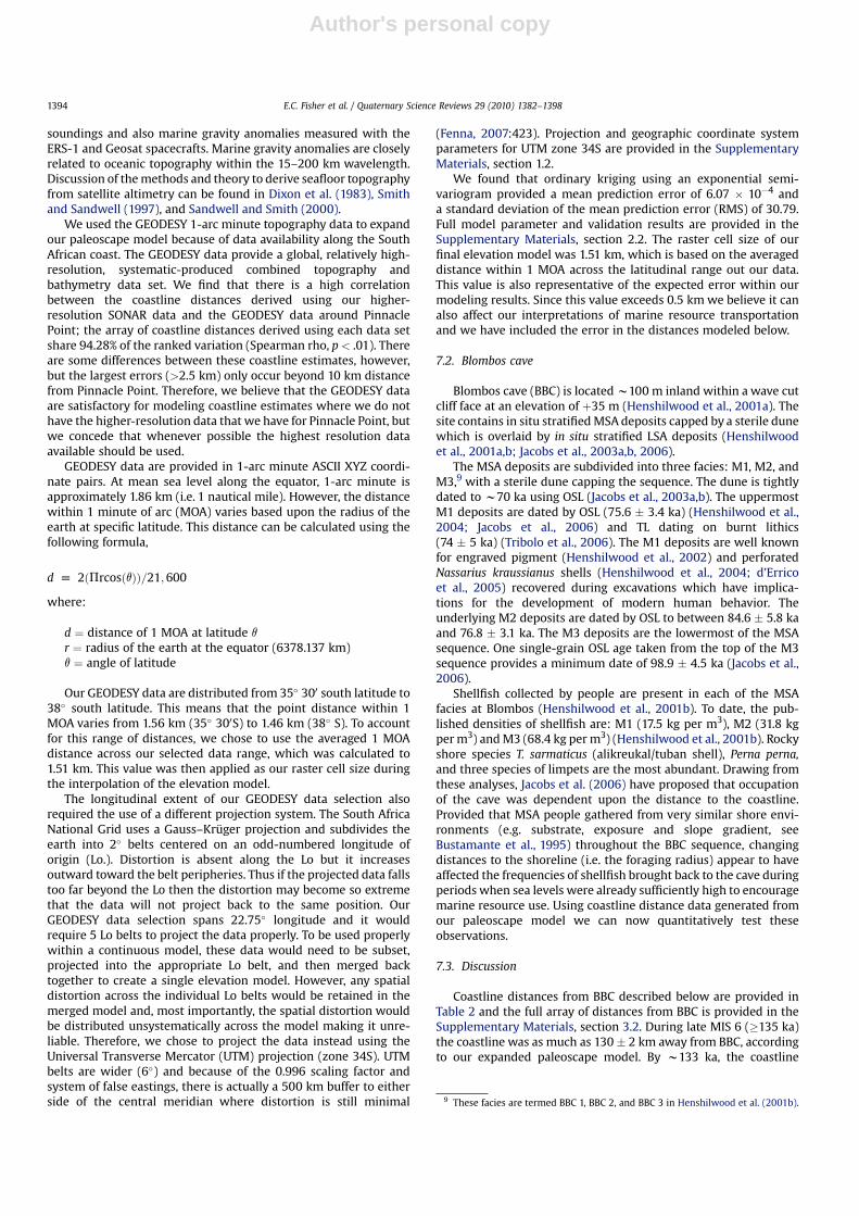
In summary, the paleoscape model accords well with thearchaeological evidence from Blombos. The correlation betweencoastline distance to the coastline and shellfish densities proposedby Jacobs et al. (2006) is also supported for the M1 and M2 faciesthrough our model results. Moreover, our results support anotherobservation made by Henshilwood et al. (2001b:442) that thecoastline must have been farther from Blombos during M1 and M2times because of the markedly higher mussel frequencies during

the accumulation of both of these facies than during M3. Musselshave been shown to be transported farther than limpets and otherspecies through both archaeological and ethnographic case studies(they keep better because they are a bivalve) (Meehan, 1982;Parkington et al., 1988). Accordingly, the greater frequencies ofshellfish seen in the M3 facies are possibly due to a nearby coast-line. A minor regression during M2 times still situated the coastlinewithin 8 km of BBC, but despite a slightly longer overall distance tothe coast a longer exposure to the coastline still can account for thefrequencies of shellfish seen in these deposits. The M1 deposits,with the least amount of shellfish may be due, in part, to a morelimited exposure to the coast only prior to 74 ka.

8. Conclusions

Recently, Bailey and Flemming (2008) have called for a morerigorous approach to studying coastal adaptations and currentlycoastal landscapes that were, in the past, significantly altered bychanging sea levels. We agree. We contend that as part of a morerigorous approach to the study of now-coastal archaeological sites thetarget should be a paleoscape model that begins with accurate andprecise reconstructions of coastline distance and configuration overtime at increments useful to understanding ancient human land use.

In the past, researchers have relied on laborious and staticapproaches to estimate coastline distance and coastline configu-ration. While our approach requires substantial time investment inthe construction of the model, once the model is created thengenerating output is easy and straightforward. Importantly, themodel is dynamic and developments in GIS, computer 3Dmodeling, and construction of sea level curves allow us to improvedramatically on prior approaches with accurate and precise coast-line distance estimates. Our model is also organic in that as ageestimates change, bathymetric data improves, and the sea levelcurves become better resolved, we can quickly improve the model.This framework provides a means to render, view, and analyze ourdata in a geometric construct more similar to the physical world inwhich we live, rather than just through tables and static figures. Butof equal importance, this framework, the model itself, and also eachdata source, can be tested, refined, and rejected, if necessary. Wethus move beyond purely graphic modeling toward a moreengaging, sensible, and modern way to understand our world, pastand present (for further, see the Supplementary Video).

Paleoscape modeling may also contribute new understanding ofthe limitations and possibilities that were likely experienced byhumans living astride coastal shelves like the Agulhas Bank duringthe Middle and Late Pleistocene. Importantly, joining the model togeophysical data could allow us to model soil, sediment, andtopography on the Agulhas Bank at specific time slices. Variation inthe current Cape Flora is strongly conditioned by rainfall amount,season of rainfall, topography, and soil conditions (Goldblatt andManning, 2002; Proches et al., 2006; Cowling et al., 2008). If wejoin our model to reconstructions of rainfall season and amount(Chase and Meadows, 2007; Lewis, 2008), we have the possibility ofmodeling floral zones on the ancient exposed continental shelf atspecific slices through time. This is the next step in our effort.

Here, we have demonstrated our beginning paleoscape modelfor Pinnacle Point and how it can relate to, and inform upon, otherindependent approaches. Our example from Blombos cave is onlyto illustrate the wide-ranging application of this model along theSouth African coast and, effectively, beyond. At present we havealso modeled coastline distances for other important MSA sitesfrom the East and West coasts of South Africa where changes in thecontinental shelf provide widely varying scenarios. These resultswill be published in the future as we continue to expand anddevelop our existing paleoscape model.

Table 2Modeled coastline distances at Blombos cave. These results accord well with faunalevidence from Blombos Cave that indicates marine resource use and support theconclusions of Jacobs et al., (2006) that shellfish collection was directly related to thedistance of the site to the coastline.

Age, ka Average distances Minimum distances Maximum distances

RLS,meters

Distance,km

RLS,meters

Distance,km

RLS,meters

Distance,km

M1 Deposits72.50 �67.31 15.56 �53.92 7.65 �80.41 43.7874.00 �44.38 7.65 �31.45 2.33 �57.45 9.4275.50 �39.62 4.10 �26.68 2.33 �52.68 7.6577.00 �36.31 2.33 �23.37 2.33 �49.37 7.6578.50 �25.43 2.33 �12.47 1.45 �38.47 4.10

M2 Deposits80.00 �19.70 2.33 �6.73 1.45 �32.73 2.3381.50 �18.67 2.33 �5.70 1.45 �31.70 2.3383.00 �22.30 2.33 �9.34 1.45 �35.34 2.3384.50 �32.06 2.33 �19.11 2.33 �45.11 7.6586.00 �41.87 4.10 �28.93 2.33 �54.93 7.6587.50 �48.63 7.65 �34.43 2.33 �61.71 9.4289.00 �48.29 7.65 �35.37 2.33 �61.37 9.4290.50 �47.19 7.65 �34.26 2.33 �60.26 9.4292.00 �42.20 7.65 �29.27 2.33 �55.27 7.6593.50 �34.74 2.33 �21.79 2.33 �47.79 7.65

M3 Deposits95.00 �27.02 2.33 �14.07 1.45 �40.07 4.1096.50 �27.59 2.33 �14.64 1.45 �40.64 4.1098.00 �27.81 2.33 �14.85 1.45 �40.85 4.1099.50 �23.84 2.33 �10.87 1.45 �36.87 2.33101.00 �20.86 2.33 �7.89 1.45 �33.89 2.33102.50 �21.18 2.33 �8.22 1.45 �34.22 2.33



Acknowledgements

The authors would like to acknowledge SAHRA and HeritageWestern Cape for providing permits to conduct excavations at theaforementioned sites and export of specimens for analysis. Wewould also like to thank the Mossel Bay community, Mossel Baymunicipality, the staff of the Dias museum, and the Cape NatureConservation.

SACP4 is funded by the National Science Foundation (US) (grants# BCS-9912465, BCS-0130713, and BCS-0524087 to Marean), theHyde Family Trust, the Institute of Human Origins at Arizona StateUniversity, and Arizona State University.

Additionally, we want to thank Dr. Tjeerd H. van Andel and Dr.Charl Bosman for providing bathymetric data around Mossel Bay,Dr. Claire Waelbroeck for providing the reconstructed RSL curvedata, and Dr. Richard Wonnacott (Director of Survey Services, ChiefDirectorate for Surveys and Mapping, South Africa) and Dr. Gren-ville Barnes (University of Florida) for providing useful geomaticinformation and suggestions relating to this study. The authors arealso very appreciative of the Institute of Social Science Research atASU for providing facilities and Jong-Geun Kim, also of the ISSR,who developed the sea level slider toolbar plugin for ESRI ArcMap.Finally, we would like to extend our appreciation to the entire MAPand SACP4 research team.

Appendix. Supplementary information

Supplementary information associated with this article can befound, in the online version, at doi:10.1016/j.quascirev.2010.01.015.

References

Ayalon, A., Bar-Matthews, M., Kaufman, A., 1999. Petrography, strontium, bariumand uranium concentrations, and strontium and uranium isotope ratios inspeleothems as palaeoclimatic proxies: Soreq Cave, Israel. The Holocene 9,715–722.

Backwell, L., d’Errico, F., 2008. Early hominid bone tools from Drimolen, SouthAfrica. Journal of Archaeological Science 35, 2880–2894.

Bailey, G.N., 2007. Coastlines, submerged landscapes, and human evolution: the RedSea Basin and the Farasan Islands. The Journal of Island and Coastal Archaeology2, 127–160.

Bailey, G.N., Craighead, A.S., 2003. Late Pleistocene and Holocene coastal palae-oeconomies: a reconsideration of the molluscan evidence from Northern Spain.Geoarchaeology 18, 175–204.

Bailey, G.N., Flemming, N.C., 2008. Archaeology of the continental shelf: marineresources, submerged landscapes and underwater archaeology. QuaternaryScience Reviews 27, 2153–2165.

Banner, J.L., Musgrove, M., Asmerom, Y., Edwards, R.L., Hoff, J.A., 1996. High-reso-lution temporal record of Holocene ground-water chemistry: tracing linksbetween climate and hydrology. Geology 24, 1049–1053.

Bar-Matthews, M., Marean, C.W., Karkanas, P., Jacobs, Z., Fisher, E., Herries, A.I.R.,Ayalon, A., Schilman, B. 2008. A high-resolution and continuous isotopic spe-loethem record of paleoclimate and paleoenvironment from 92–55 ka fromPinnacle Point, South Africa. The Annual Meeting of the PaleoanthropologySociety. Vancouver, British Columbia, March 25–March 26, 2008.

Bar-Matthews, M., Ayalon, A., Kaufman, A., Wasserburg, G.J., 1999. The EasternMediterranean paleoclimate as a reflection of regional events: Soreq cave,Israel. Earth and Planetary Science Letters 166, 85–95.

Binford, L.R., 1980. Willow smoke and dogs tails: hunter-gatherer settlementsystems and archaeological site formation. American Antiquity 45, 4–20.

Binford, L.R., 1982. The archaeology of place. Journal of Anthropological Archae-ology 1, 5–31.

Birch, G.F.D.P.A., Du Plessis, A., Willis, J.P., 1978. Offshore and onland geological andgeophysical investigations in the Wilderness Lakes region. Transactions of theGeological Society of South Africa 81, 339–352.

Bird, E.C.F., 2000. Coastal Geomorphology: An Introduction. John Wiley, Chichester.Bird, D.W., Bliege-Bird, R.L., 1997. Contemporary shellfish gathering strategies

among the Meriam of the Torres Strait Islands, Australia: testing predictions ofa central place foraging model. Journal of Archaeological Science 24, 39–63.

Bird, D.W., Richardson, J.L., Veth, P.M., Barham, A.J., 2002. Explaining shellfishvariability in middens on the Meriam Islands, Torres Strait, Australia. Journal ofArchaeological Science 29, 457–469.

Bradley, R.S., 1999. Paleoclimatology: Reconstructing Climates of the Quaternary.Academic Press, San Diego.

Brown, K.S., Marean, C.W., Herries, A.I.R., Jacobs, Z., Tribolo, C., Braun, D.,Roberts, D.L., Meyer, M.C., Bernatchez, J., 2009. Fire as an engineering tool ofearly modern humans. Science 325, 859–862.

Buchanan, W.F., Parkington, J.E., Robey, T.S., and Vogel, J.C., 1984. Shellfish, subsis-tence and settlement: some western Cape Holocene observations, 121–130.

Bustamante, R.H., Branch, G.M., Eekhout, S., Robertson, B., Zoutendyk, P.,Schleyer, M., Dye, A., Hanekom, N., Keats, D., Jurd, M., McQuaid, C.D., 1995.Gradients of intertidal productivity around the coast of South Africa and theirrelationship with consumer biomass. Oecologia 102, 189–201.

Caputo, R., 2007. Sea-level curves: perplexities of an end-user in morphotectonicapplications. Global and Planetary Change 57, 417–423.

Chappell, J., Omura, A., Esat, T., McCulloch, M., Pandolfi, J., Ota, Y., Pillans, B., 1996.Reconciliation of late Quaternary sea levels derived from coral terraces at HuonPeninsula with deep sea oxygen isotope records. Earth and Planetary ScienceLetters 141, 227–236.

Chappell, J., Shackleton, N.J., 1986. Oxygen isotopes and sea level. Nature 324,137–140.

Chase, B.M., Meadows, M.E., 2007. Late Quaternary dynamics of southern Africa’swinter rainfall zone. Earth Science Reviews 84, 103–138.

Cowling, S.A., Cox, P.M., Jones, C.D., Maslin, M.A., Peros, M., Spall, S.A., 2008.Simulated glacial and interglacial vegetation across Africa: implications forspecies phylogenies and trans-African migration of plants and animals. GlobalChange Biology 14, 827–840.

Cowling, R.M., Proches, S., 2005. Patterns and evolution of plant diversity in theCape Floristic Region. Biologiske Skrifter 55, 273–288.

Deacon, J., Lancaster, N., 1988. Late Quaternary Paleoenvironments of SouthernAfrica. Clarendon Press, Oxford.

Dixon, T.H., Naraghi, M., McNutt, M.K., Smith, S.M., 1983. Bathymetric predictionfrom SEASAT Altimiter data. Journal of Geophysical Research-Oceans andAtmospheres 88, 1563–1571.

Ehrlich, S., Gavrieli, I., Dor, L.B., Halicz, L., 2001. Direct high-precision measurementsof the Sr-87/Sr-86 isotope ratio in natural water, carbonates and relatedmaterials by multiple collector inductively coupled plasma mass spectrometry(MC-ICP-MS). Journal of Analytical Atomic Spectrometry 16, 1389–1392.

Erlandson, J.M., 2001. The archaeology of aquatic adaptations: paradigms for a newmillennium. Journal of Archaeological Research 9, 287–350.

d’Errico, F., Henshilwood, C., Vanhaeren, M., van Niekerk, K., 2005. Nassariuskraussianus shell beads from Blombos cave: evidence for symbolic behaviour inthe Middle Stone Age. Journal of Human Evolution 48, 3–24.

Fagundes, N.J.R., Ray, N., Beaumont, M., Neuenschwander, S., Salzano, F.M.,Bonatto, S.L., Excoffier, L., 2007. Statistical evaluation of alternative models ofhuman evolution. Proceedings of the National Academy of Sciences 104,17614–17619.

Fenna, D., 2007. Cartographic Science: a Compendium of Map Projections withDerivations. CRC Press, New York.

Flemming, B.W., 1983. Sediment dynamics on the inner Agulhus bank. SouthAfrican Journal of Science 79, 160–160.

Flemming, B.W., Martin, A.K., Rogers, J., 1983. Onshore and offshore coastal aeo-lianites between Mossel Bay and Knysna. University of Cape Town MarineGeoscience, Unit Technical Report No. 14, pp. 151–160.

Frumkin, A., Stein, M., 2004. The Sahara-East Mediterranean dust and climateconnection revealed by strontium and uranium isotopes in a Jerusalem spe-leothem. Earth and Planetary Science Letters 217, 451–464.

Goede, A., McCulloch, M., McDermott, F., Hawkesworth, C., 1998. Aeolian contri-bution to strontium and strontium isotope variations in a Tasmanian speleo-them. Chemical Geology 149, 37–50.

Goldblatt, P., 1997. Floristic diversity in the Cape flora of South Africa. Biodiversityand Conservation 6, 359–377.

Goldblatt, P., Manning, J.C., 2002. Plant diversity of the Cape region of southernAfrica. Annals of the Missouri Botanical Garden 89, 281–302.

Gonder, M.K., Mortensen, H.M., Reed, F.A., de Sousa, A., Tishkoff, S.A., 2007. Whole-mtDNA genome sequence analysis of ancient African lineages. MolecularBiology and Evolution 24, 757–768.

Grine, F.E., 1998. Additional human fossils from the Middle Stone Age of Die KeldersCave 1, South Africa:1995 excavation. South African Journal of Science 94,229–235.

Grun, R., Beaumont, P., Tobias, P.V., Eggins, S., 2003. On the age of Border Cave 5human mandible. Journal of Human Evolution 45, 155–167.

Haas, J.D., Harrison, G.G., 1977. Nutritional anthropology and biological adaptation.Annual Review of Anthropology 6, 69–101.

Halicz, L., Segal, I., Fruchter, N., Stein, M., Lazar, B., 2008. Strontium stable isotopesfractionate in the soil environments? Earth and Planetary Science Letters 272,406–411.

Hearty, P.J., Hollin, J.T., Neumann, A.C., O’Leary, M.J., McCulloch, M., 2007. Global sea-level fluctuations during the Last Interglaciation (MIS 5e). Quaternary ScienceReviews 26, 2090–2112.

Hendey, Q.B., Volman, T.P., 1986. Last interglacial sea levels and coastal caves in theCape Province, South Africa. Quaternary Research 2, 189–198.

d’Errico, F., Henshilwood, C.S., 2007. Additional evidence for bone technology in thesouthern African Middle Stone Age. Journal of Human Evolution 52, 142–163.

Henshilwood, C.S., Nilssen, P., Parkington, J., 1994. Mussel drying and food storage inthe late Holocene, SW Cape, South Africa. Journal of Field Archaeology 21,103–109.

Henshilwood, C.S., D’Errico, F., Marean, C.W., Milo, R.G., Yates, R.J., 2001a. An earlybone tool industry from the Middle Stone Age, Blombos Cave, South Africa:



implications for the origins of modern human behaviour, symbolism andlanguage. Journal of Human Evolution 41, 631–678.

Henshilwood, C.S., Sealy, J.C., Yates, R.J., Cruz-Uribe, K., Goldberg, P., Grine, F.E.,Klein, R.G., Poggenpoel, C., van Niekerk, K., Watts, I., 2001b. Blombos cave,southern Cape, South Africa: preliminary report on the 1992–1999 excavationsof the Middle Stone Age levels. Journal of Archaeological Science 28, 421–448.

Henshilwood, C.S., d’Errico, F., Yates, R., Jacobs, Z., Tribolo, C., Duller, G.A.T.,Mercier, N., Sealy, J.C., Valladas, H., Watts, I., Wintle, A.G., 2002. Emergence ofmodern human behavior: Middle Stone Age engravings from South Africa.Science 295, 1278–1280.

Henshilwood, C., d’Errico, F., Vanhaeren, M., van Niekerk, K., Jacobs, Z., 2004. MiddleStone Age shell beads from South Africa. Science 304, 404.

Imbrie, J., Hays, J.D., Martinson, D.G., McIntyre, A., Mix, A.C., Morley, J.J., Pisias, N.G.,Prell, W.L., Shackleton, N.J., 1984. The orbital theory of Pleistocene climate:-support from a revised chronology of the marine d18O record. In: Palisades, N.Y.,Berger, A., Imbrie, J., Hays, H., Kukla, G., Saltzman, B. (Eds.), Milankovitch andClimate: Understanding the Response to Astronomical Forcing. Proceedings ofthe NATO Advanced Research Workshop Held 30 November–4 December, 1982.D. Reidel Publishing, Dordrecht.

Ingman, M., Kaessmann, H., Paabo, S., Gyllensten, U., 2000. Mitochondrial genomevariation and the origin of modern humans. Nature 408, 708–713.

Jacobs, Z. An OSL chronology for the sedimentary deposits from Pinnacle Point Cave13B – a punctuated presence. Journal of Human Evolution, submitted forpublication.

Jacobs, Z., Duller, G.A.T., Wintle, A.G., 2003a. Optical dating of dune sand fromBlombos Cave, South Africa: II–single grain data. Journal of Human Evolution44, 613–625.

Jacobs, Z., Wintle, A.G., Duller, G.A.T., 2003b. Optical dating of dune sand fromBlombos Cave, South Africa: I–multiple grain data. Journal of Human Evolution44, 599–612.

Jacobs, Z., Duller, G.A.T., Wintle, A.G., Henshilwood, C.S., 2006. Extending thechronology of deposits at Blombos Cave, South Africa, back to 140 ka usingoptical dating of single and multiple grains of quartz. Journal of HumanEvolution 51, 255–273.

Jacobs, Z., Roberts, R.G., Galbraith, R.F., Deacon, H.J., Grun, R., Mackay, A.,Mitchell, P., Vogelsang, R., Wadley, L., 2008. Ages for the Middle Stone Age ofSouthern Africa: implications for human behavior and dispersal. Science 322,733–735.

Jacobs, Z., Roberts, R.G., 2007. Advances in optically stimulated luminescence datingof individual grains of quartz from archaeological deposits. EvolutionaryAnthropology 16, 210–223.

Jerardino, A., 2003. Pre-colonial settlement and subsistence along sandy shoressouth of Elands Bay, West Coast, South Africa. South African ArchaeologicalBulletin 58, 53–62.

Jerardino, A., Marean, C.W. Shellfish gathering, marine palaeoecology and modernhuman behavior: perspectives from cave PP13b, Pinnacle Point, South Africa.Journal of human evolution, in press.

Jouzel, J., Hoffmann, G., Parrenin, F., Waelbroeck, C., 2002. Atmospheric oxygen 18and sea-level changes. Quaternary Science Reviews 21, 307–314.

Kelly, R.L., 1983. Hunter-gatherer mobility strategies. Journal of AnthropologicalResearch 39, 277–306.

Kelly, R.L., 1995. The Foraging Spectrum. Smithsonian Institution Press, Washington,DC.

Klein, R.G., 1972. The late quaternary mammalian fauna of Nelson Bay Cave (CapeProvince, South Africa): its implications for megafaunal extinctions and envi-ronmental and cultural change. Quaternary Research 2, 135–142.

Klein, R.G., 1976. The mammalian fauna of the Klasies River mouth sites, southernCape Province, South Africa. South African Archaeological Bulletin 31, 75–98.

Klein, R.G., Deacon, H.J., Hendey, Q.B., Lambrechts, J.J.N., 1983. Palaeoenvironmentalimplications of Quaternary large mammals in the fynbos region. In:Deacon, H.J., Hendey, Q.B., Lambrechts, J.J.N. (Eds.), Fynbos Palaeoecology:a Preliminary Synthesis. South African National Scientific Programmes, CSIR, pp.116–138. SANSP Report 75.

Lambeck, K., Esat, T.M., Potter, E.K., 2002. Links between climate and sea levels forthe past three million years. Nature 419, 199–206.

Lee, R.B., 1972. Kung spatial organization: an ecological and historical perspective.Human Ecology 1, 73–97.

Lee, R.B., Lee, R.B., DeVore, I., 1968. What hunters do for a living, or, how to makeout on scarce resources. In: Lee, R.B., DeVore, I. (Eds.), Man the Hunter. Aldine,Chicago, pp. 30–48.

Lewis, C.A., 2008. Late Quaternary climatic changes, and associated humanresponses, during the last w45,000 yr in the Eastern and adjoining WesternCape, South Africa. Earth Science Reviews 88, 167–187.

Mackay, A., Welz, A., 2008. Engraved ochre from a Middle Stone Age context at KleinKliphuis in the Western Cape of South Africa. Journal of Archaeological Science35, 1521–1532.

Malan, J.A., 1987. The Bredasdorp group in the area between Gans Bay and MosselBay. South African Journal of Science 83, 506–507.

Malan, J.A., 1991. Lithostratigraphy of the Klein Brak formation (Bredarsdorp group).In: South African Committee for Stratigraphy: Lithostratigraphic Series.Department of Mineral and Energy Affairs, Geological Survey, pp. 1–13.

Marean, C.W., 2000. The Middle Stone Age at Die Kelders Cave 1, South Africa.Journal of Human Evolution 38, 3–5.

Marean, C.W., Assefa, Z., 2005. The middle and upper Pleistocene African record for thebiological and behavioral origins of modern humans. In: Stahl, A. (Ed.), African

Archaeology: a Critical Introduction. Blackwell Publishing Ltd, New York, pp. 93–129.

Marean, C.W., Nilssen, P.J., Brown, K., Jerardino, A., Stynder, D., 2004. Paleoanthro-pological investigations of Middle Stone Age sites at Pinnacle point, Mossel Bay(South Africa): archaeology and hominid remains from the 2000 field season.Paleoanthropology 2, 14–83.

Marean, C.W., Bar-Matthews, M., Bernatchez, J., Fisher, E., Goldberg, P., Herries, A.I.R.,Jacobs, Z., Jerardino, A., Karkanas, P., Minichillo, T., Nilssen, P.J., Thompson, E.,Watts, I., Williams, H.M., 2007. Early human use of marine resources and pigmentin South Africa during the Middle Pleistocene. Nature 449, 905–908.

Marean, C.W., Bar-Matthews, M., Fisher, E.C., Goldberg, P., Herries, A., Karkanas, P.,Nilssen, P., Thompson, E.. The stratigraphy of the Middle Stone Age sediments atPinnacle Point Cave 13B (Mossel Bay, western Cape Province, South Africa).Journal of Human Evolution, in press.

Marker, M.E., 1984. Marine benches of the Eastern Cape, South Africa. Transactionsof the Geological Society of South Africa 87, 11–18.

Marker, M.E., 1987. A note on marine benches of the southern Cape. South AfricanJournal of Geology 90, 120–123.

Martinson, D.G., Pisias, N., Hays, J.D., Imbrie, J., Moore Jr., T.C., Shackleton, N.J., 1987.Age dating and the orbital theory of the ice ages: development of a high-resolution 0–300,000-year chronostratigraphy. Quaternary Research 27, 1–29.

McBrearty, S., Brooks, A.S., 2000. The revolution that wasn’t: a new interpretation ofthe origin of modern human behavior. Journal of Human Evolution 39,453–563.

McDougall, I., Brown, F.H., Fleagle, J.G., 2005. Stratigraphic placement and age ofmodern humans from Kibish, Ethiopia. Nature 433, 733–736.

Meehan, B., 1982. Shell Bed to Shell Midden. Australian Institute of AborginalStudies, Atlantic Highlands.

Musgrove, M., Banner, J.L., 2004. Controls on the spatial and temporal variability ofvadose dripwater geochemistry: Edwards aquifer, central Texas. Geochimica etCosmochimica Acta 68, 1007–1020.

Olson, S.L., Hearty, P.J., 2009. A sustained þ21 m sea-level highstand during MIS 11(400 ka): direct fossil and sedimentary evidence from Bermuda. QuaternaryScience Reviews 28, 271–285.

Parkington, J., Poggenpoel, C., Buchanan, W., Robey, T., Manhire, T., Sealy, J.,Bailey, G., Parkington, J., 1988. Holocene coastal settlement patterns in theWestern Cape. In: Bailey, G., Parkington, J. (Eds.), The Archaeology of PrehistoricCoastlines. Cambridge Univ. Press, NY, pp. 22–41.

Proches, S., Cowling, R.M., Goldblatt, P., Manning, J.C., Snijman, D.A., 2006. Anoverview of the Cape geophytes. Biological Journal of the Linnean Society 87,27–43.

Ramsay, P.J., Cooper, J.A., 2002. Late Quaternary sea-level change in South Africa.Quaternary Research 57, 82–90.

Rightmire, G.P., Deacon, H.J., Schwartz, J.H., Tattersall, I., 2006. Human foot bonesfrom Klasies River main site, South Africa. Journal of Human Evolution 50,96–103.

Sandwell, D.T., Smith, W.H.F., 2000. Bathymetric estimation. In: Fu, L.-L.,Cazenave, A., Holton, G.A. (Eds.), Satellite Altimetry and Earth Sciences:a Handbook of Techniques and Applications. International Geophysics Series.Academic Press, San Diego, pp. 441–456.

Shackleton, N.J., 1987. Oxygen isotopes, ice volume and sea level. QuaternaryScience Reviews 6, 183–190.

Shackleton, N.J., Opdyke, N.D., 1973. Oxygen isotope and palaeomagnetic stratig-raphy of equatorial pacific core V28–238: oxygen isotope temperatures and icevolumes on a 10/5 year and 10/6 year scale. Quaternary Research 3, 39–55.

Silberbauer, G.B., 1981. Hunter and Habitat in the Central Kalahari Desert. Cam-bridge University Press, Cambridge.

Smith, W.H.F., Sandwell, D.T., 1997. Global sea floor topography from satellitealtimetry and ship depth soundings. Science 277, 1956–1962.

Tanaka, J., 1980. The San Hunter-Gatherers of the Kalahari: a Study in EcologicalAnthropology. University of Tokyo Press, Tokyo.

Tribolo, C., Mercier, N., Selo, M., Valladas, H., Joron, J.L., Reyss, J.L., Henshilwood, C.,Sealy, J., Yates, R., 2006. TL dating of burnt lithics from Blombos Cave (SouthAfrica): further evidence for the antiquity of modern human behaviour.Archaeometry 48, 341–357.

Tribolo, C., Mercier, N., Valladas, H., Joron, J.L., Guibert, P., Lefrais, Y., Selo, M.,Texier, P.J., Rigaud, J.P., Porraz, G., Poggenpoel, C., Parkington, J., Texier, J.P.,Lenoble, A., 2009. Thermoluminescence dating of a Stillbay-Howiesons Poortsequence at Diepkloof Rock Shelter (Western Cape, South Africa). Journal ofArchaeological Science 36, 730–739.

USGS, 2004. Shuttle Radar Topography Mission, 3 Arc Seconds SceneSRTM_u03_p172r084, Unfilled Unfinished 2.0. In: Global Land Cover ChangeFacility. University of Maryland, College Park, Maryland.

Van Andel, T.H., 1989. Late Pleistocene sea levels and the human exploitation of theshore and shelf of southern south Africa. Journal of Field Archaeology 16,133–155.

Verhyden, S., Keppens, E., Fairchild, I.J., McDermott, F., Weis, D., 2000. Mg, Sr and Srisotope geochemistry of Belgian Holocene speleothems: implications for pale-oclimate reconstructions. Chemical Geology 169, 131–144.

Vogel, J.C., Tobias, P.V., Raath, M.A., Maggi-Cecchi, J., Doyle, G.A., 2001. Radiometricdates for the Middle Stone age in South Africa. In: Tobias, P.V., Raath, M.A.,Maggi-Cecchi, J., Doyle, G.A. (Eds.), Humanity from African Naissance to ComingMillennia. Florence University Press, Florence, pp. 261–268.

Waelbroeck, C., Labeyrie, L., Michel, E., Duplessy, J.C., McManus, J.F., Lambeck, K.,Balbon, E., Labracherie, M., 2002. Sea-level and deep water temperature



changes derived from benthic foraminifera isotopic records. Quaternary ScienceReviews 21, 295–305.

Watts, I., 2002. Ochre in the Middle Stone Age of southern Africa: ritualized displayor hide preservative? South African Archaeological Bulletin 57, 1–14.

Watts, I., Dunbar, R., Knight, C., Power, C., 1999. The origin of symbolic culture. In:Dunbar, R., Knight, C., Power, C. (Eds.), The Evolution of Culture. EdinburghUniversity Press, Edinburgh, pp. 113–146.

White, T.D., Asfaw, B., DeGusta, D., Gilbert, H., Richards, G.D., Suwa, G., Howell, F.C.,2003. Pleistocene Homo sapiens from middle Awash, Ethiopia. Nature 423,742–747.

de Wit, M., 2007. The Kalahari epeirogeny and climate change: differentiating causeand effect from core to space. South African Journal of Geology 110, 367–392.

Woodroffe, C.D., 2003. Coasts: Form, Process, and Evolution. Cambridge UniversityPress, New York.


Middle and Late Pleistocene paleoscape modeling along the southern coast of South Africa

Documents

Transcript of Middle and Late Pleistocene paleoscape modeling along the southern coast of South Africa