JOURNAL OF GEOPHYSICAL RESEARCH, VOL. 100, NO. C8, PAGES 16,029-16,044, AUGUST 15, 1995

Buoy observations of the atmosphere along the west coast of the United States, 1981-1990

Clive E. Dorman and Clinton D. Winant

Center for Coastal Studies, Scripps Institution of Oceanography, University of California, San Diego, La Jolla

Abstract. The distribution of statistical properties of the meteorological and sea surface temperature fields along the west coast of the United States is described based on 10-yearlong observations from buoys deployed by the National Data Buoy Center. The observations suggest that properties vary differently in each of three different regions along the coast: the Southern California Bight which remains sheltered from strong wind forcing throughout the year; the central and northern California coast up to Cape Mendocino, the site of persistent equatorward winds; and the Oregon-Washington coast, where traveling cyclones and anticyclones produce vigorous and variable forcing. Over most of the region the variance in the wind speed is roughly equally divided between the annual cycle and the synoptic forcing, corresponding to periods between 5 and 50 cycles per year. Two seasons, summer and winter, are sufficient to describe the annual cycle. During the summer, two distinct wind speed maxima occur along the coast, one near Point Conception and the other off northern California, between Point Reyes and Point Arena. In the winter a single maximum occurs, located near Point Conception. The atmospheric pressure generally increases with latitude along the coast, but the annual cycle of atmospheric pressure has a different phase, depending on location; off the coast of California, highest pressures are found during the winter, while off Oregon and Washington, the highest pressures occur during the summer. Fluctuations in air and sea temperature are highly correlated, and the sea temperature is usually higher than the air temperature, in the winter. Examination of vertical soundings of the atmosphere at Oakland, Vandenberg Air Force Base and San Diego during the same period of time reveals that a well-defined inversion separates the marine boundary layer (MBL) from the free atmosphere above nearly 90% of the time during the summer and half the time during the winter. Station soundings consistently overestimate the MBL thickness, but the results do suggest that the MBL is supercritical part of the time in the vicinity of the three sites. An attempt is made to examine the interannual variability and compare it to the Southern Oscillation index, although the results are limited because the record length is short compared with interannual timescales. Spatially averaged temperature anomalies increase during winter 1982-1983, coincident with the large E1 Nifio event.

1. Introduction

The western seaboard of the continental United States has

been described as a classical upwelling area. It is located at midlatitudes and is under the influence of the North Pacific

subtropical high, over the eastern Pacific, and is also influenced by the thermal low which develops over the southwestern United States during the summer. Neiburger et al. [1961] have described the vertical structure of the summer

atmosphere in this area as being characterized by a strong temperature inversion between cool and moist air in a marine boundary layer (MBL)and the subsiding dry and warmer air in the free atmosphere above. The thickness of the MBL ranges between 300 and 400 m along the Pacific coast, depending on location, and rises toward the west, reaching an altitude of

Copyright 1995 by the American Geophysical Union.

Paper number 95JC00964. 0148-0227/95/95 JC- 00964505.00

2000 m near Hawaii. During the summer the MBL thickness has been observed to vary between 50 and 800 m.

Nelson [1977] provided the first detailed description of surface wind stress over the coastal waters adjacent to the west coast of the continental United States based on surface marine

observations provided by ships. Most observations were collected after 1950, although some date back to the mid- 19th century. During the months of June and July, maximum wind stresses in excess of 0.15 Pa are found in the area between Cape Mendocino and Point Reyes (Figure 1) and extending several hundred kilometers offshore. In this area the stress is directed

equatorward and thus is favorable to upwelling during the spring and summer. Along the coast of southern and Baja California the wind stress is described as favorable for

upwelling throughout the year, but with weaker amplitudes than along the northern California coast.

Halliwell and Allen [1987] (hereinafter referred to as HA)

examined the large-scale coastal wind field along the west coast of North America for the summer of 1981 and 1982 and

16,029

16,030 DORMAN AND WINANT: BUOY OBSERVATIONS ALONG THE U.S. WEST COAST

B41

B29

B40

B27

B22

B30

B14

B13

B26

B12

B42

B28

Bll

B23

B25

B24

N

••F• cape

ttery - Washington _

• Oregon _ ( Cape -

,( Cape_

-•ndocino _ • Northern

ß •:, Arena California - ß '•g. IF't• Reyes - •'•Oakland -

•._•-- San

ß "•Francisco - Central •, Sur _ California ß •

ß • Vandenberg -

ß _t••ception

Southern . % '• California ß ß •San - "'"_' ....... I•Diego

Bight •:--- - I I I I I I I I I I Mex' 32 ø

126 ø 124 ø 122 ø 120 ø 118 ø

48 ø

46 ø

44 ø

42 ø

40 ø

38 ø

36 ø

34 ø

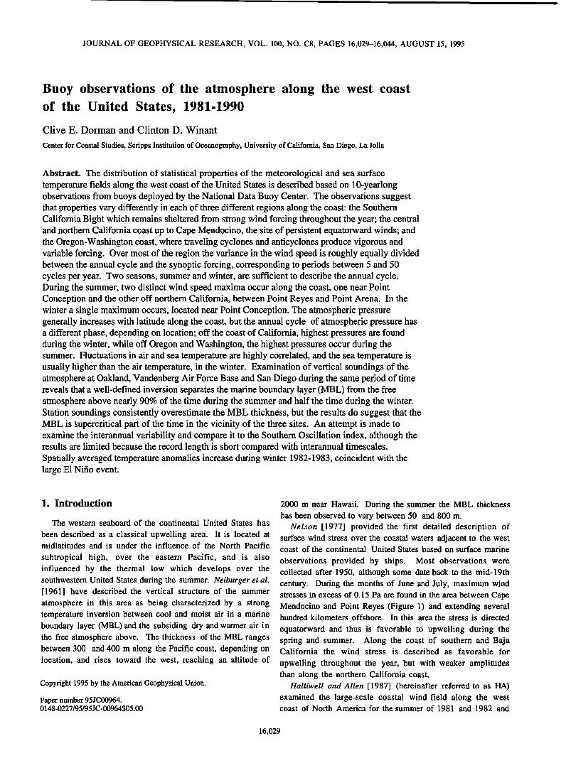
Figure 1. The west coast of the continental United States, showing the location of the National Data Buoy Corporation (NDBC) buoys and free balloon release sites.

the intervening winter, using observed and computed winds. In this analysis, summer wind fluctuations were found to be driven by the combined North Pacific high and the southwest thermal low, with some influence exercised by propagating atmospheric systems to the north of the area. In the winter, wind fluctuations are driven primarily by the propagating cyclones and anticyclones and have larger variance and space scales than in the summer. Wind fluctuations are reported to

propagate equatorward during the winter and poleward during the summer.

At times during the summer, when the upwelling favorable winds are interrupted, the marine layer thickens. Intrusions of dense air have been observed to propagate up the coast confined vertically by the inversion and laterally by the Coriolis trapping against the coastal mountain range [Dorman, 1985, 1987, 1988; Mass and Allbright, 1987, 1988]. The scale analysis of Overland [1984] demonstrates that for such an . vicinity of Point Conception.

event the momentum balance in the direction parallel to the coast is expected to be ageostrophic and the momentum balance in the direction perpendicular to the coast is expected to be geostrophic. These equations can result in either linear or nonlinear solutions. Reason and Steyn [1992] use a nonlinear semigeostrophic theory to show that propagating events correspond to an alongshore ageostrophic downgradient flow, and that either solitary Kelvin waves or shock Kelvin waves are associated with the intrusion. Typical propagation speeds range between 4.0 and 6.5 m s -]. Mass and Allbright [1987] also suggest that in some cases the transitions can be associated with synoptic scale changes and lee-troughing due to the synoptic scale flow.

During the summer months the stable MBL and the free atmosphere above can be represented as a one and a half layer reduced gravity hydraulic flow. Winant et al [1988] have noted that after equatorward winds have been established for a few days the Froude number which characterizes the MBL can exceed one and the MBL behaves as a supercritical layer, accelerating when the flow boundaries expand and generating hydraulic jumps when the flow is compressed. Sarnelson [1992] proposed a numerical model consisting of a homogeneous rotating fluid layer, forced by upper level pressure gradients and including the effect of surface friction. The results suggest that supercritical features such as expansion fans are to be expected when the flow is supercritical, although they may be altered by frictional effects. Hydraulic jumps are shown to weaken rapidly with distance offshore, consistent with the increasing MBL height, upstream of the jump.

Regional climatological descriptions are available which describe the circulation over shorter timescales. Between

Point Arena and San Francisco, Beardsley et al. [1987} describe the structure of the atmospheric boundary layer during the summer months. The MBL is capped by a strong inversion, and the vertical structure of the lower atmosphere is stable. The North Pacific high and the thermal low that develops over the southwestern United States during late spring and summer combine to produce steady equatorward winds over this area. At the same time the MBL is very thin, typically in the range between 30 and 150 m. Periods of weak or reversed winds occur when trapped disturbances propagate poleward along the coast. The MBL thickness then increases to between 600 and 800 m. These wind relaxations are not

normally associated with a weakening of the large-scale pressure systems. During the winter, Domtan et al. [1995] have shown that the inversion is not well defined, the

atmosphere is more frequently unstable, and the wind direction can be either up- or downcoast.

Near Point Conception, at the border between central and southern California, the properties of the lower atmosphere during the spring and summer have been described by Brink and Muench [1986] and by Caldwell et al. [1986]. This is an area characterized by large spatial gradients in the wind field, as the strong equatorward flow which occurs along the coast of northern and central California separates from the coast in the

Within the Santa Barbara

DORMAN AND WINANT: BUOY OBSERVATIONS ALONG THE U.S. WEST COAST 16,031

Channel area, diurnal variability is important, but the amplitude of the diurnal fluctuations depends on the synoptic conditions.

The lower atmosphere off southern California, between Point Conception and San Diego, is described by the U.S. Navy [1971] and by Dorman [1982]. During the spring and summer this is an area which is sheltered from the equatorward winds that characterize the rest of the California coast. During the winter the area is also sheltered from the cyclones which

produce vigorous winds along the coast, north of Point Conception. In the summer the MBL is capped by a stable inversion, generally at a higher altitude than off northern California. During the winter the inversion is not as well defined as in the summer, but the atmosphere is usually stable. Santa Ana winds, directed offshore, occur from fall through

spring, resulting from the combined influence of the large- scale high-pressure system which develops at that time over the great basin (Colorado and Nevada)and a low which develops to the west of southern California.

The existence of 10 years of observations of meteorological variables as well as sea surface temperature (SST) data from buoys moored in the ocean, far from the obstacles which characterize land stations, makes it possible to describe the distribution of mean atmospheric flow properties and SST along the coast. Previous descriptions have been based on ship observations, with attendant sampling problems, or relatively short records at a fixed station.

Table 1. Location of Observation Stations and Orientation

of the Coastline

Station Latitude Longitude Coast N W Orientation

deg

NDBC 41 47ø24 ' 124ø30 ' 150

NDBC 29 46ø12 ' 124ø12 ' 173

NDBC 40 44ø48 ' 124ø18 ' 175

NDBC 27 41 o48' 124o24 ' 165

NDBC 22 40ø48 ' 124ø30 ' 177

NDBC 30 40ø24 ' 124ø30 ' 170

NDBC 14 39ø12 ' 124ø00 ' 153

NDBC 13 38o12 ' 123o18 ' 130

NDBC 26 37o48 ' 122o42 ' 130

NDBC 12 37o24 ' 122o42 ' 153

NDBC 42 36o48 ' 122o24 ' 150

NDBC 28 35o48 ' 121 o54' 145

NDBC 11 34o54 ' 120o54 ' 147

NDBC 23 34ø18' 120o42 ' 147

NDBC 25 33ø42 ' 119ø06 ' 110

NDBC 24 32048 ' 119012 ' 138

2. The Observations

In 1981 the first elements of an array of meteorological buoys on the west coast of the continental United States were deployed by the National Data Buoy Center (NDBC) under the sponsorship of the Minerals Management Service (MMS). This array of platforms provides the first opportunity to describe the atmospheric field over the coastal ocean free from questions associated with effects of land obstacles. Accordingly, the results included here are based solely on measurements from the buoys and exclude any land-based observations. The buoys are located within a Rossby radius of deformation from the coast and thus feel the steering effect of

coastal topography, but they are sufficiently far from the coast that the observations are not affected by microscale land features.

The position of the NDBC buoys [National Oceanic and Atmospheric Administration 1992] used in this study is listed in Table 1 and illustrated in Figure 1. The buoys were distributed irregularly along the coast, with a higher density of buoys deployed along the central and northern California coast than along the coasts of Washington-Oregon or in the Southern California Bight (SCB). While, in general, the buoys were moored over the continental shelf, neither the water depth nor the distance from the coast was maintained constant. The orientation of the coastline closest to the buoy is included in

Table 1, as previous analyses (e.g., HA) have shown that the wind is usually polarized in a direction parallel to the coast.

The buoys were all instrumented to measure wind speed and direction, atmospheric pressure, and air and sea temperature

measured 1 m beneath the surface. The accuracy of the wind

speed sensor, as reported by Hamilton [1980] is +1 m s -1, the accuracy of the direction sensor is +10 ø, the accuracy of the barometric pressure sensor is +1 hPa, and the air and sea temperature observations have an accuracy of +1 øC.

The height at which the wind observations were made depends on the buoy and payload configuration used, varies from location to location, and varies in time at any location,

as different buoys were moved to a given location in the course of the deployment. The different platforms deployed off the west coast include 3-m discuss buoys, 6-m Navy Oceanograph- ic and Meteorological Automated Device (NOMAD) buoys, and 10- and 12-m discuss buoys [Hamilton, 1980]. Individual observations of wind speed and direction provided by NDBC include the height at which the measurement was made, ranging between 5 and 13.8 m. In order to compare these observa- tions, a standard height of 10 m above sea level was selected, and 10-m observations were computed from the measure. ments assuming a logarithmic wind profile as given by Panofsky and Dutton [1984]

U. Z

u = • In--- (1) Zo

where u is the wind speed at height z, u. is the friction

velocity, k a is the von Karman constant, taken to be 0.41, and

zo is reference height. The friction velocity is given by taken

to be 0.41, and zo is reference height. The friction velocity is

given by

16,032 DORMAN AND WINANT: BUOY OBSERVATIONS ALONG TIlE U.S. WEST COAST

B13

B41

B29

B40

B27

B22

B30

B14

B26

B12

B42

B28

Bll

B23

B25

B24

1981 82 83 84 85 86 87 88 89 90 91 Year

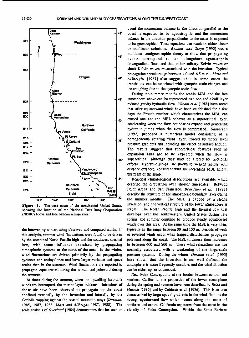
Figure 2. Data coverage for the various buoys deployed along the U.S. west coast by NDBC, 1981-1990.

2

U* 2 = C D UlO (2)

where U]o is the speed at 10 m. Given the speed at any height

z, (1) and (2) can be solved iteratively, given the drag coefficient CD. It should be noted that the constant z 0 does not

enter in the computation of the ratio of wind amplitude at

different heights. Values of CD given by Large and Pond

[1981 ] for a neutral atmosphere were used. Over the period of deployment, several gaps of varying

lengths occurred at each station. In the case when gaps were shorter than 2 days, observations were estimated by linear interpolation. For longer gaps, no effort was made to replace the missing observations, except to estimate spectral properties as described in section 3. The resulting coverage for each station, after filling in the short gaps, is illustrated in Figure 2. In all cases, hourly observations are used, although at different stages of the analysis, higher-frequency fluctuations are removed, either by means of filtering or by eliminating periodic (annual) components.

3. Means and Variance Spectra

Statistical properties of the 10-m winds, the barometric pressure, and the air and sea temperature at the 16 locations are summarized in Table 2 and illustrated in Figure 3. Average values are computed using all observations, excluding the gaps described earlier.

Two options are available to describe the statistics of a vector quantity such as the horizontal wind over some time period. The wind can be described by amplitude (speed) and direction relative to some arbitrary direction, say north, and the means and higher-order moments of the speed and direction can be computed. Alternatively, the horizontal wind can be described in terms of two components in a coordinate system

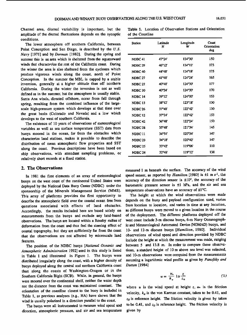
Table 2. Mean and Standard Deviation Statistics for the Wind, Atmospheric Pressure, Air and Sea Temperature Observed at the Different Buoy Locations Along the U.S. West Coast, 1981-1990

,

Mean Wind Wind Principal Axes Atmospheric Pressure, Air Temperature, Sea Temperature, hPa 'C 'C

Station ' ' Speed, Direction, Direction, Major Minor Mean Standard Mean Standard Mean Standard ms-] 'T North øT North Deviation Deviation Deviation

,

NDBC 41 0.6 48 144 5.4 3.0 1017.8 6.7 10.7 2.8 11.6 2.2

NDBC 29 0.6 1 174 5.3 4.2 1017.4 7.7 10.4 3.1 10.9 2.5

NDBC 40 0.6 97 174 6.0 3.2 1019.0 5.9 11.5 2.7 12.0 2.1

NDBC 27 1.5 159 162 6.8 2.8 1018.5 5.5 10.8 2.0 10.8 1.5

NDBC 22 1.3 158 176 6.3 2.5 1018.0 5.6 11.6 2.0 11.8 1.5

NDBC 30 2.3 161 164 6.6 2.3 1018.0 5.2 10.8 1.9 10.8 1.3

NDBC 14 3.0 151 151 6.4 2.1 1017.1 5.1 11.9 1.8 12.2 1.6

NDBC 13 4.5 129 128 6.0 2.5 1017.4 4.7 11.9 1.9 11.8 1.7

NDBC 26 2.9 113 127 4.7 2.9 1017.3 4.7 12.1 2.0 12.7 1.7

NDBC 12 3.0 139 152 5.1 2.3 1017.4 4.7 12.9 1.8 13.5 1.5

NDBC 42 4.3 146 146 4.9 2.3 1017.7 4.4 12.6 1.8 13.2 1.5

NDBC 28 5.5 142 143 5.3 1.7 1017.6 4.1 13.5 1.7 13.9 1.6

NDBC 11 4.8 144 144 4.4 2.1 1016.2 4.0 13.6 1.9 14.1 1.8

NDBC 23 6.5 145 145 4.8 2.0 1016.0 3.8 14.2 1.9 14.5 1.9

NDBC 25 2.3 114 116 3.5 2.5 1015.3 3.8 16.2 2.4 17.3 2.4

NDBC 24 5.4 128 136 3.9 1.9 1014.8 3.5 15.7 2.3 16.8 2.3 ß

DORMAN AND WINANT: BUOY OBSERVATIONS ALONG THE U.S. WEST COAST 16,033

t > E 5 ß •

Pt. Cape Conception Mendocino

(a)

(b)

150

IO0

5O

0 (c)

'•' 1020

• 1018

: 1016

• 1014

,• 2o

. 15

E

• 10 32

i i i i ! i

34 36 38 40 42 44 46 Latitude (øN)

(d)

(e) 48

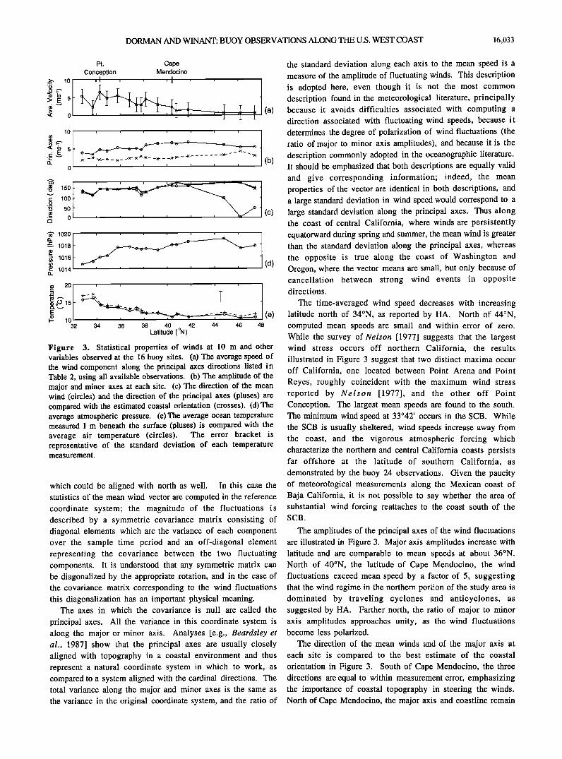
Figure 3. Statistical properties of winds at 10 m and other variables observed at the 16 buoy sites. (a) The average speed of the wind component along the principal axes directions listed in Table 2, using all available observations. (b) The amplitude of the major and minor axes at each site. (c) The direction of the mean wind (circles) and the direction of the principal axes (pluses) are compared with the estimated coastal orientation (crosses). (d)The average atmospheric pressure. (e)The average ocean temperature measured 1 m beneath the surface (pluses) is compared with the average air temperature (circles). The error bracket is representative of the standard deviation of each temperature measurement.

which could be aligned with north as well. In this case the statistics of the mean wind vector are computed in the reference coordinate system; the magnitude of the fluctuations is described by a symmetric covariance matrix consisting of diagonal elements which are the variance of each component over the sample time period and an off-diagonal element representing the covariance between the two fluctuating components. It is understood that any symmetric matrix can be diagonalized by the appropriate rotation, and in the case of the covariance matrix corresponding to the wind fluctuations this diagonalization has an important physical meaning.

The axes in which the covariance is null are called the

principal axes. All the variance in this coordinate system is along the major or minor axis. Analyses [e.g., Beardsley et al., 1987] show that the principal axes are usually closely aligned with topography in a coastal environment and thus represent a natural coordinate system in which to work, as compared to a system aligned with the cardinal directions. The total variance along the major and minor axes is the same as the variance in the original coordinate system, and the ratio of

the standard deviation along each axis to the mean speed is a measure of the amplitude of fluctuating winds. This description is adopted here, even though it is not the most common description found in the meteorological literature, principally because it avoids difficulties associated with computing a

direction associated with fluctuating wind speeds, because it determines the degree of polarization of wind fluctuations (the ratio of major to minor axis amplitudes), and because it is the description commonly adopted in the oceanographic literature. It should be emphasized that both descriptions are equally valid and give corresponding information; indeed, the mean properties of the vector are identical in both descriptions, and a large standard deviation in wind speed would correspond to a large standard deviation along the principal axes. Thus along the coast of central California, where winds are persistently

equatorward during spring and summer, the mean wind is greater than the standard deviation along the principal axes, whereas the opposite is true along the coast of Washington and Oregon, where the vector means are small, but only because of cancellation between strong wind events in opposite directions.

The time-averaged wind speed decreases with increasing latitude north of 34øN, as reported by HA. North of 44øN, computed mean speeds are small and within error of zero. While the survey of Nelson [1977] suggests that the largest wind stress occurs off northern California, the results

illustrated in Figure 3 suggest that two distinct maxima occur off California, one located between Point Arena and Point

Reyes, roughly coincident with the maximum wind stress reported by Nelson [1977], and the other off Point

Conception. The largest mean speeds are found to the south. The minimum wind speed at 33042 ' occurs in the SCB. While the SCB is usually sheltered, wind speeds increase away from the coast, and the vigorous atmospheric forcing which characterize the northern and central California coasts persists far offshore at the latitude of southern California, as

demonstrated by the buoy 24 observations. Given the paucity of meteorological measurements along the Mexican coast of Baja California, it is not possible to say whether the area of substantial wind forcing teattaches to the coast south of the SCB.

The amplitudes of the principal axes of the wind fluctuations are illustrated in Figure 3. Major axis amplitudes increase with latitude and are comparable to mean speeds at about 36øN. North of 40øN, the latitude of Cape Mendocino, the wind fluctuations exceed mean speed by a factor of 5, suggesting that the wind regime in the northern port:'on of the study area is dominated by traveling cyclones and anticyclones, as suggested by HA. Farther north, the ratio of major to minor axis amplitudes approaches unity, as the wind fluctuations become less polarized.

The direction of the mean winds and of the major axis at each site is compared to the best estimate of the coastal orientation in Figure 3. South of Cape Mendocino, the three directions are equal to within measurement error, emphasizing the importance of coastal topography in steering the winds. North of Cape Mendocino, the major axis and coastline remain

16,034 DORMAN AND WINANT: BUOY OBSERVATIONS ALONG THE U.S. WEST COAST

parallel, even though the mean direction does not. As the mean wind speed is much less than the amplitude of the major axis, the direction of the mean wind is probably not significant north of 42øN.

Mean atmospheric pressure generally increases with latitude, and the steepest gradient is located between southern California and 36øN. While average and fluctuating pressure differences between the buoys are significant, their in{erpration in terms of gradients is difficult, since the locations of the different buoys do not correspond to any natural coordinate system. These pressure differences probably result from a varying combination of along- and across- streamline gradients.

Time averages of the air and sea temperature decrease with increasing latitude. The sea temperature exceeds the air temperature, implying a sensible heat flux from the ocean toward the atmosphere. The difference varies with location along the coast; it is largest in the SCB and smallest off northern California, where the upwelling process, driven by the equatorward wind during spring and summer, brings cold water to the surface.

The long time series analyzed here provide the opportunity to describe the spectral characteristics of the wind field over a wide range of frequencies. Observations from the buoy NDBC 13, located between San Francisco and Point Arena, are

selected since that station is about midway along the span of coast resolved bY the measurements and is exposed to some of the largest mean winds. Given the polarization of the wind field in the direction parallel to the coast, attention is restricted to wind fluctuations along the major axis.

Wind observations at NDBC 13 constitute a nearly continuous record, although some gaps exist. Spectral estimates are easier to estimate from continuous records, and

for these analyses, gaps in the NDBC 13 major axis wind record were filled using major axis wind observations from the closest buoy, NDBC 14. The amplitude of the latter fluctuations were adjusted by using the regression coefficient computed from periods when measurements were available at both stations. During the month of March 1990, neither station provided wind measurements. The gap in NDBC

10 0 ..-

10-4

10.2

10 .3

10-4

10-s 10-4 10 ø 10 • 10 :• 10 3 1 O n

Frequency (cpy)

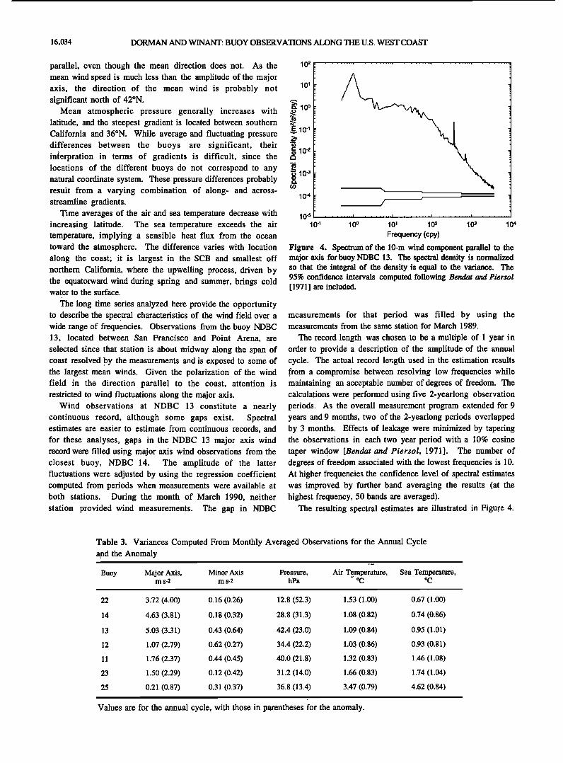
Figure 4. Spectrum of the 10-m wind component parallel to the major axis for buoy NDBC 13. The spectral density is normalized so that the integral of the density is equal to the variance. The 95% confidence intervals computed following Bendat and Piersol [1971 ] are included.

measurements for that period was filled by using the measurements from the same station for March 1989.

The record length was chosen to be a multiple of 1 year in order to provide a description of the amplitude of the annual cycle. The actual record le-,gth used in the estimation results .from a compromise between resolving low frequencies while maintaining an acceptable number of degrees of freedom. The calculations were performed using five 2-yearlong observation periods. As the overall measurement program extended for 9 years and 9 months, two of the 2-yearlong periods overlapped by 3 months. Effects of leakage were minimized by tapering the observations in each two year period with a 10% cosine taper window [Bendat and Piersol, 1971]. The number of degrees of freedom associated with the lowest frequencies is 10. At higher frequencies the confidence level of spectral estimates was improved by further band averaging the results (at the highest frequency, 50 bands are averaged).

The resulting spectral estimates are illustrated in Figure 4.

Table 3. Variances Computed From Monthly Averaged Observations for the Annual Cycle and the Anomaly

Buoy Major Axis, Minor Axis Pressure, Air Te•mperature, Sea Temperature, m $-2 m s-2 hPa øC øC

22 3.72 (4.00) 0.16 (0.26) 12.8 (52.3) 1.53 (1.00) 0.67 (1.00)

14 4.63 (3.81) 0.18 (0.32) 28.8 (31.3) 1.08 (0.82) 0.74 (0.86)

13 5.03 (3.31) 0.43 (0.64) 42.4 (23.0) 1.09 (0.84) 0.95 (1.01)

12 1.07 (2.79) 0.62 (0.27) 34.4 (22.2) 1.03 (0.86) 0.93 (0.81)

11 1.76 (2.37) 0.44 (0.45) 40.0 (21.8) 1.32 (0.83) 1.46 (1.08)

23 1.50 (2.29) 0.12 (0.42) 31.2 (14.0) 1.66 (0.83) 1.74 (1.04)

25 0.21 (0.87) 0.31 (0.37) 36.8 (13.4) 3.47 (0.79) 4.62 (0.84)

Values are for the annual cycle, with those in parentheses for the anomaly.

DORMAN AND WINANT: BUOY OBSERVATIONS ALONG THE U.S. WEST COAST 16,035

The spectrum is normalized so that the integral under the spectrum is equal to the variance of the major axis wind fluctuations. The spectrum exhibits a significant peak at one cycle per year (cpy), corresponding to the annual cycle. The existence of this peak is consistent with previous descriptions of the atmosphere in this area [Strub et al., 1987]. This spectrum is similar to the spectra wind stress modulus observation at weather station C [Willebrand, 1978], which is also characterized by a significant peak at the annual period and an energetic continuum at periods between 100 and 10 days. In the present case the spectrum is relatively flat in the range of frequencies between 5 and 50 cpy, corresponding to synoptic forcing and longer periods. Over these frequencies the spectral estimates are characteristic of a wideband random process. Estimates of the amplitude of the seasonal component of the wind described in section 8 and Table 3 suggest that the total variance in the major axis wind fluctuations is approximately equally divided between the annual cycle and the extended synoptic band. This motivates the following description of the fluctuations: the annual cycle is characterized in section 4, and synoptic changes are reported in section 5. At higher frequencies, distinct peaks appear at the diurnal (one cycle in 24 hours) and semidiurnal (one cycle in 12 hours) frequencies. While all observed variables fluctuate on a daily basis, the variance associated with the diurnal band is small compared to the total variance resolved by these observations. Remaining analyses of the time series are based on observations filtered using the PL64 low-pass filter [Limeburner, 1985] which removes almost all the energy at periods shorter than 38 hours.

4. The Annual Cycle and Seasons

Spectra of 10-yearlong time series of wind fluctuations suggest that about half the variance in the wind field is accounted for by the annual cycle. In order to describe this cycle for the different locations, monthly averaged values for each variable are computed as the average for each calendar month during tb.e period of available observations. Thus the average and standard deviation of all pressure observations during the month of February at NDBC 13 in the course of the 10-year span are used to form an average and a standard deviation of pressure at that site for February. Wind vectors were projected along the direction of the principal axes listed in Table 2, and the average and standard deviation of each component was computed as for a scalar.

The monthly averaged wind vectors for each site and for each month are illustrated in Figure 5. North of Cape Blanco (buoys 41, 29, and 40), monthly averaged winds are weak, as most of the variability occurs on synoptic timescales, shorter than 1 month, but the directions follow a consistent pattern, generally equatorward and parallel to the coast during the summer and poleward during the winter. South of Cape Mendocino, the amplitude of the summer monthly averages increases with decreasing latitude under the persistent influence of the North Pacific high. South of Point Sur (buoys 24, 25, 23, 11, and 28), the direction of the monthly averaged wind

•5 m/s

i i i i i i I i i i i .

Jan Mar May July Sep Month

Figure 5. Annual cycle of the wind.

Nov

B41 l/

B29 •

B40 •

B27 Iil

B22 {I

B30 I I

B14 I/

B13 I•

B26 I•'

B12 If I

B42 I/

B28 I/

Bll l/

B23 i•

B25 L•,

B 24

For each location the

vertical direction corresponds to the direction of the principal axes listed in Table 2. The relative orientation of that direction

from north is sketched on the right-hand side, with the vector pointing toward north. The locations of the buoys are given in Table 1.

vector remains equatorward throughout the year. The largest monthly averaged speeds are observed at Point Conception. The weak monthly averages observed in the SCB (buoy 23) are consistent with the year-round sheltering described previously. Strub et al. [1987] described the seasonal cycles of currents, temperature, winds, and sea level in the same area based on observations spanning the period 1981-1983 and report a similar latitudinal progression of seasonal wind stresses, although the yearlong average wind stress computed off the Washington coast for the 1981-1983 period is large and directed toward the north, whereas the results presented here suggest that the yearly averaged wind stress off Washington is small compared with fluctuations, and the direction is not well defined. This disagreement could be due to the different selection of observation stations. The Strub et al. [1987]

study was based, for the most part, on land-based measurements or could reflect atypical conditions for 1981-1983.

Principal axes of the wind fluctuations over a month are illustrated in Figure 6. The variability of the wind field over a month is always greater in wintertime, when weather is governed by traveling systems. This progression is

16,036 DORMAN AND WINANT: BUOY OBSERVATIONS ALONG THE U.S. WEST COAST

5m/s

IT

T / T I I

I I I I I I I I

I m i z

B41 •

B29 i•

B40 •

B27 •

B22 •

B30 •

B14 •

B13 •'

B26 L.•

B12 •

B42 •

B28 •

Bll IX

B23 •

B25 L•'

B24 l ,• , I , I , I , I , I , I , I ! I , I , I , I ,

Jan Mar May July Sep Nov Month

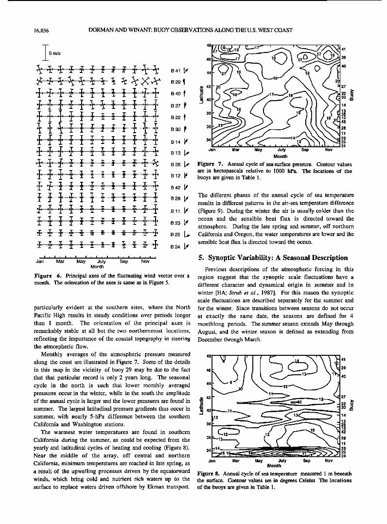
Figure 6. Principal axes of the fluctuating wind vector over a month. The orientation of the axes is same as in Figure 5.

particularly evident at the southern sites, where the North Pacific High results in steady conditions over periods longer than 1 month. The orientation of the principal axes is remarkably stable at all but the two northernmost locations, reflecting the importance of the coastal topography in steering the atmospheric flow.

Monthly averages of the atmospheric pressure measured as along the coast are illustrated in Figure 7. Some of the details in this map in the vicinity of buoy 29 may be due to the fact as that that particular record is only 2 years long. The seasonal cycle in the north is such that lower monthly averaged 44 pressures occur in the winter, while in the south the amplitude

ß 42

of the annual cycle is larger and the lower pressures are found in •

summer. The largest latitudinal pressure gradients thus occur in • n0 summer, with nearly 5-hPa difference between the southern California and Washington stations. as

The warmest water temperatures are found in southern California during the summer, as could be expected from the as yearly and latitudinal cycles of heating and cooling (Figure 8). an Near the middle of the array, off central and northern California, minimum temperatures are reached in late spring, as a result of the upwelling processes driven by the equatorward winds, which bring cold and nutrient rich waters up to the surface to replace waters driven offshore by Ekman transport.

46 • 1 29

• 42 27 = , 1•8 • 17 22 •' .• 40 30 I•

14

13 38 26

12 42

36 28 11

34 23 25

' ' ' ' ' ' 24 Jan Mar May July Sep Nov

Month

Figure 7. Annual cycle of sea surface pressure. Contour values are in hectopascals relative to 1000 hPa. The locations of the buoys are given in Table 1.

The different phases of the annual cycle of sea temperature results in different patterns in the air-sea temperature difference (Figure 9). During the winter the air is usually colder than the ocean and the sensible heat flux is directed toward the

atmosphere. During the late spring and summer, off northern California and Oregon, the water temperatures are lower and the sensible heat flux is directed toward the ocean.

5. Synoptic Variability: A Seasonal Description

Previous descriptions of the atmospheric forcing in this region suggest that the synoptic scale fluctuations have a different character and dynamical origin in summer and in winter [HA; Strub et al., 1987]. For this reason the synoptic scale fluctuations are described separately for the summer and for the winter. Since transitions between seasons do not occur

at exactly the same date, the seasons are defined for 4 monthlong periods. The summer season extends May through August, and the winter season is defined as extending from December through March.

41

29

40

27

22 0

30 m 14

13 26 12 42

28

11

23 25 24

Jan Mar May July Sep Nov Month

Figure 8. Annual cycle of sea temperature measured 1 m beneath the surface. Contour values are in degrees Celsius The locations of the buoys are given in Table !.

DORMAN AND WINANT: BUOY OBSERVATIONS ALONG THE U.S. WEST COAST 16,037

•40

27

12

42

28

-- 23 34 5 25

24 Jan Mar May July Sep Nov

Month

Figure 9. Annual cycle of monthly averaged difference between sea and air temperatures. Contour values are in degrees Celsius. The locations of the buoys are given in Table 1.

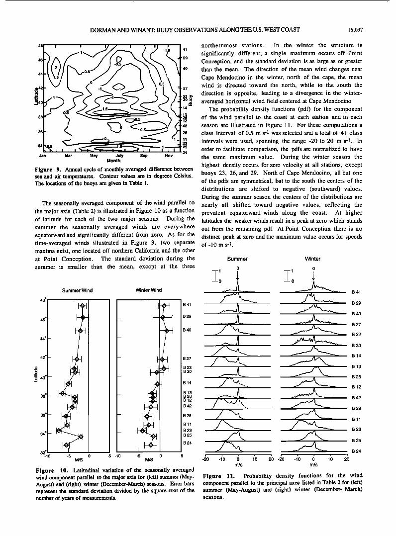
The seasonally averaged component of the wind parallel to the major axis (Table 2) is illustrated in Figure 10 as a function of latitude for each of the two major seasons. During the summer the seasonally averaged winds are everywhere equatorward and significantly different from zero. As for the time-averaged winds illustrated in Figure 3, two separate maxima exist, one located off northern California and the other at Point Conception. The standard deviation during the summer is smaller than the mean, except at the three

Summer Wind Winter Wind

48 ø

-- -- I '• 3 I I

44 ø -- _

42 ø -- -- I

I'•11

I I I I

32 ø • -10 -5 0 5 -10 -5 0 5

M/S M/S

B41

B 29

B 40

B 27

B 22 B 30

B14

B13 B 26 B12

B 42

B 28

Bll

B 23 B 25

B 24

Figure 10. Latitudinal variation of the seasonally averaged wind component parallel to the major axis for (left) summer (May- August) and (right) winter (December-March) seasons. Error bars represent the standard deviation divided by the square root of the number of years of measurements.

northernmost stations. In the winter the structure is

significantly different; a single maximum occurs off Point Conception, and the standard deviation is as large as or greater than the mean. The direction of the mean wind changes near Cape Mendocino in the winter, north of the cape, the mean wind is directed toward the north, while to the south the

direction is opposite, leading to a divergence in the winter- averaged horizontal wind field centered at Cape Mendocino.

The probability density functions (pdf) for the component of the wind parallel to the coast at each station and in each season are illustrated in Figure 11. For these computations a class interval of 0.5 m s -1 was selected and a total of 41 class

intervals were used, spanning the range -20 to 20 m s-1. In order to facilitate comparison, the pdfs are normalized to have the same maximum value. During the winter season the highest density occurs for zero velocity at all stations, except buoys 23, 26, and 29. North of Cape Mendocino, all but one of the pdfs are symmetrical, but to the south the centers of the distributions are shifted to negative (southward)values. During the summer season the centers of the distributions are nearly all shifted toward negative values, reflecting the prevalent equatorward winds along the coast. At higher latitudes the weaker winds result in a peak at zero which stands out from the remaining pdf. At Point Conception there is no distinct peak at zero and the maximum value occurs for speeds of-10 m s-•.

Summer Winter

o o

; ; B41

B 29

B 40

B 27

B 22

b 30

B14

B13

B 26

B12

B 42

B 28

Bll

B 23

B 25

B 24

-•0 -1'0 (• 1'0 '•'0 -:•0 -1'0 (• 1;3 2•) m/s m/s

Figure 11. Probability density functions for the wind component parallel to the principal axes listed in Table 2 for (left) summer (May-August) and (fight) winter (December- March) seasons.

16,038 DORMAN AND WINANT: BUOY OBSERVATIONS ALONG • U.S. WEST COAST

Sea Temperature

48 ø

44 ø -

40 ø -

36 ø -

32 ø 6

Ii .... * .... Winter • Summer

- B41

- B29

- B40

- B27

- B22

- B30

- B14

- B13 - B26 - B12

- B42

- B28

- Bll

- B23

- B25

- B24

I I I

14 22

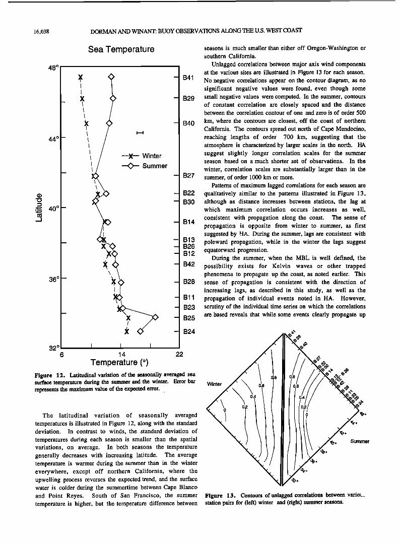
Temperature (o) Figure 12. Latitudinal variation of the seasonally averaged sea surface temperature during the summer and the winter. Error bar represents the maximum value of the expected error.

seasons is much smaller than either off Oregon-Washington or southern California.

Unlagged correlations between major axis wind components at the various sites are illustrated in Figure 13 for each season. No negative correlations appear on the contour diagram, as no significant negative values were found, even though some small negative values were computed. In the summer, contours of constant correlation are closely spaced and the distance between the correlation contour of one and zero is of order 500

kin, where the contours are closest, off the coast of northern

California. The contours spread out north of Cape Mendocino, reaching lengths of order 700 km, suggesting that the atmosphere is characterized by larger scales in the north. HA suggest slightly longer correlation scales for the summer season based on a much shorter set of observations. In the

winter, correlation scales are substantially larger than in the summer, of order 1000 km or more.

Patterns of maximum lagged correlations for each season are qualitatively similar to the patterns illustrated in Figure 13, although as distance increases between stations, the lag at which maximum correlation occurs increases as well,

consistera with propagation along the coast. The sense of propagation is opposite from winter to summer, as first suggested by HA. During the summer, lags are consistent with poleward propagation, while in the winter the lags suggest equatorward progression.

During the summer, when the MBL is well defined, the possibility exists for Kelvin waves or other trapped phenomena to propagate up the coast, as noted earlier. This sense of propagation is consistent with the direction of increasing lags, as described in this study, as well as the propagation of individual events noted in HA. However, scrutiny of the individual time series on which the correlations are based reveals that while some events clearly propagate up

Winter

The latitudinal variation of seasonally averaged temperatures is illustrated in Figure 12, along with the standard deviation. In contrast to winds, the standard deviation of

temperatures during each season is smaller than the spatial variations, on average. In both seasons the temperature generally decreases with increasing latitude. The average temperature is warmer during the summer than in the winter everywhere, except off northern California, where the upwelling process reverses the expected trend, and the surface water is colder during the summertime between Cape Blanco and Point Reyes. South of San Francisco, the summer temperature is higher, but the temperature difference between

0.2

Summer

Figure 13. Contours of un!agged correlations between vatlot__ station pairs for (left) winter and (fight) summer seasons.

DORMAN AND WINANT: BUOY OBSERVATIONS ALONG TI-IE U.S. WEST COAST 16,039

the coast, in many cases, no sense of propagation can be ccnsistently determined. The pattern of increasing lags thus represents an average picture which does not correspond closely to any individual realization. The different nature of fluctuation patterns along the coast during the summer can be explained, at least in part, by the fact that the usually equatorward winds which characterize this area may relax to weak winds in at least two different ways. Trapped disturbances in the marine layer are expected to progress poleward. Synoptic disturbances such as upper level anticyclones or offshore flows aloft can also cause the winds to weaken. Under

some conditions these synoptic conditions may propagate, although not necessarily in a direction parallel to the coast.

During the winter the lags for which maximum correlation occurs between pairs of buoy observations establish a pattern of southern propagation. As the subsidence which characterizes the summertime high-pressure system is absent, the MBL is not as well defined, and fluctuations in the wind

field are driven by propagating cyclones and anticyclones. The most energetic events are commonly associated with

6. Relationships Between Parameters

The long time series obtained by NDBC provide the opportunity of defining the transfer function between the various parameters measured at each station, as a function of frequency. Cross spectra between the various observations from buoy 13 are used to define these transfer functions. For

this analysis the gaps in buoy 13 measurements longer than 2 days were filled with measurements from buoy 14, as described for the wind major axis observations in section 3. The coherence, phase, and gain functions between pairs of time series were computed following Bendat and Piersol [1971]. The spectral estimations were derived using the sampling windows described in section 3.

The transfer function relating air and sea temperature is illustrated in Figure 14a. The coherence between this pair of variables is significantly different from zero at all frequencies resolved up to the semidiurnal frequency. The phase between the two signals •.s wi•,hin error of zero for all frequencies where the coherence is significant. The gain function, computed

cyclonic disturbances which originate in the Gulf of Alaska and using the sea temperature as input, is unity for periods near 1 propagate toward the east or southeast. year and decreases to about a half that in t•e synoptic band.

0.8

0.4 0.2

Air-Sea Temp. Wind-Sea Temp. Wind-Air Temp.

(a) i I i

(b) (c)

0

100

50

-50 -100

-150

1.5

0.5

.

I i I I

. --

..

I i I

I i t i t I

1 10 100 1000

Frequency (½py) 1 10 100 1000 1 10 100 1000

Figure 14. Frequency dependent transfer functions for three pairs of observations at buoy 13. The step line in the coherence frame indicates the coherence level above which true coherence is different from zero at the 95%

confidence level. (a) Air temperature-sea temperature, with a positive phase indicating the air temperature leads the sea temperature. (b) Wind-sea temperature, with a positive phase indicating the wind leads the sea temperature. (c) Wind-air temperature, with a positive phase indicating wind fluctuations lead the air temperature fluctuations.

16,040 DORMAN AND WINANT: BUOY OBSERVATIONS ALONG TIlE U.S. WEST COAST

Thus when the ocean temperature changes by IøC in the synoptic band, the air temperature changes by 0.5øC in response to that input.

The transfer function relating wind fluctuations along the major ax•s to sea temperature changes is illustrated in Figure 14b. The coherence between these observations is significant

at the annual period and in the synoptic band, where it exceeds the coherence between the other two pairs of measurements. At the annual period the water temperature leads the wind by 80 ø (corresponding to 80 days). The annual cycle of winds and temperature, described above, suggests that the wind reaches maximum negative values during the summer and the water temperature reaches minimum values at the same time. However, the temperature increases rapidly thereafter, as soon as the upwelling favorable winds relax, and the heat due to solar radiation is retained in the coastal zone. Maximum water

temperatures are attained in early fall, whereas maximum monthly averaged winds (in the poleward direction)occur during the winter. This timing difference explains the phase lag noted at the annual period.

In the synoptic band the phase difference is approximately 60 ø, with wind leading the temperature. The gain function computed using wind as the input paramater varies with frequency. The amplitude is such that a 0.2øC change would result from a 1 m s -1 change in the wind. These results and the high coherence between the wind and the water temperature suggest that temperature changes are directly forced by the wind, through the upwelling mechanism, in this band of frequencies.

The major axis wind fluctuations and the air temperature fluctuations are significantly coherent at the annual period and in the synoptic band of frequencies (Figure 14c), but the coherence between the two variables is significantly less than in either of the other two cases. These results suggest that the

air temperature is not directly related to wind, but rather, that the wind determines the sea temperature by means of the upwelling process and that local exchanges between the air and surface waters account for a significant amount of the air temperature variability.

7. Soundings

Vertical soundings of temperature are reported twice a day from three stations in the same area covered by the buoys. The stations are located at San Diego, at Vandenberg Air Force Base, near Point Conception, and at Oakland, near San Francisco. The soundings are made twice each day using free balloon radiosondes. The observations include pressure, wind

speed and direction, air temperature and dew point as a function of altitude. The heights for which measurements are available consist of a number of mandatory altitudes as well as other significant levels.

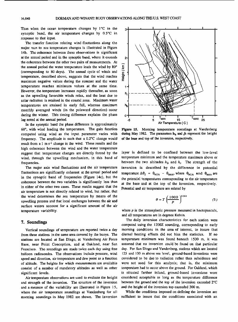
Air temperature observations are used to evaluate the height and strength of the inversion. The structure of the inversion and a measure of the variability are illustrated in Figure 15, where the air temperature soundings at Vandenberg for all morning soundings in May 1982 are shown. The inversion

I 3 I I I

2

1

ht

i , , -5 5 TMON 15

! I

' I

TMAX 25 Air Temperature ( C )

Figure 15. Morning temperature soundings at Vandenberg during May 1982. The parameters h b and t h represent the height of the base and top of the inversion, respectively.

layer is defined to be confined between the low-level

temperature minimum and the temperature maximum above or between the two altitudes h b and ht. The strength of the

inversion is described by the difference in potential

temperature AO i = 0mi n - 0max, where 0atin and 8atax are

the potential temperatures corresponding to the air temperature at the base and at the top of the inversion, respectively. Potential and air temperature are related by

1000 )0.286 o=r (3) P

where p is the atmospheric pressure measured in hectopascals, and all temperatures are in degrees Kelvin.

The daily inversion characteristics for each station were computed using the 1200Z sounding, corresponding to early morning conditions in the area of interest, to insure that diurnal heating effects did not bias the statistics. If no temperature minimum was found beneath 1500 m, it was assumed that no inversion could be found on that particular day. For San Diego and Vandenberg, stations which are located 125 and 100 m above sea level, ground-based inversions were considered to be due to radiation rather than subsidence and

were not used for this analysis; that is, the minimum temperature had to occur above the ground. For Oakland, which is situated farther inland, ground-based inversions were considered acceptable as long as the temperature difference between the ground and the top of the inversion exceeded 2øC and the height of the inversion top exceeded 300 m.

While the conditions imposed on defining the inversion are sufficient to insure that the conditions associated with an

DORMAN AND WINANT: BUOY OBSERVATIONS ALONG THE U.S. WEST COAST 16,041

lOOO

.•. 5oo

._•

ß ß

ß ß

I I 500 1000

Inversion Height at Oakland (rn)

1500

Figure 16. Corresponding values of the thickness of the marine boundary layer, as determined from free balloon soundings at Oakland (abcissa) and from aircraft soundings over the ocean in the vicinity of buoy 13.

inversion are, in fact, due to subsidence rather than an artifact

of radiation, they also preclude finding subsidence-induced low-level inversion, as described by Zernba and Friehe [1987]. The methods used here to describe the inversion are thus biased

to higher inversion heights. During the Coastal Ocean Dynamics Experiment an instrumented aircraft was used to map the properties of the MBL and to profile the atmospheric boundary layer. Observations of the vertical structure of the MBL near buoy 13 as measured by the aircraft, are presented by Friehe and Winant [1983]. The height of the MBL, as determined from the aircraft soundings, is compared with the height determined from the free balloons released at Oakland in Figure 16. The regression between 15 pairs of observations suggests that the MBL height at Oakland is always greater than over the water; the ratio of the two varies between two and three.

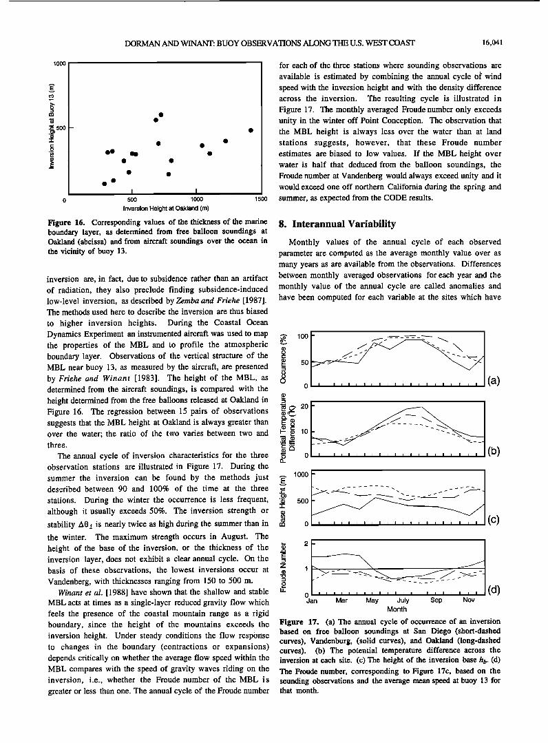
The annual cycle of inversion characteristics for the three observation stations are illustrated in Figure 17. During the

summer the inversion can be found by the methods just described between 90 and 100% of the time at the three

stations. During the winter the occurrence is less frequent,

although it usually exceeds 50%. The inversion strength or stability A0i is nearly twice as high during the summer than in the winter. The maximum strength occurs in August. The height of the base of the inversion, or the thickness of the inversion layer, does not exhibit a clear annual cycle. On the basis of these observations, the lowest inversions occur at

Vandenberg, with thicknesses ranging from 150 to 500 m. Winant et al. [1988] have shown that the shallow and stable

MBL acts at times as a single-layer reduced gravity flow which feels the presence of the coastal mountain range as a rigid boundary, since the height of the mountains exceeds the inversion height. Under steady conditions the flow response to changes in the boundary (contractions or expansions) depends critically on whether the average flow speed within the MBL compares with the speed of gravity waves riding on the inversion, i.e., whether the Froude number of the MBL is

greater or less than one. The annual cycle of the Froude number

for each of the three stations where sounding observations are available is estimated by combining the annual cycle oJ' wind speed with the inversion height and with the density difference across the inversion. The resulting cycle is illustrated in Figure 17. The monthly averaged Froude number only exceeds unity in the winter off Point Conception. The observation that the MBL height is always less over the water than at land stations suggests, however, that these Froude number estimates are biased to low values. If the MBL height over water is half that deduced from the balloon soundings, the Froude number at Vandenberg would always exceed unity and it would exceed one off northern California during the spring and summer, as expected from the CODE results.

8. Interannual Variability

Monthly values of the annual cycle of each observed parameter are computed as the average monthly value over as many years as are available from the observations. Differences between monthly averaged observations for each year and the monthly value of the annual cycle are called anomalies and have been computed for each variable at the sites which have

lOO

50

'• 20

OF. lO

ci:5 '• 0

1 ooo

500 •

0 i , • ,

(a)

(b)

(c)

ot,, ,,,, ,, ,,, Jan Mar May July Sep Nov

Month

Figure 17. (a) The annual cycle of occurrence of an inversion based on free balloon soundings at San Diego (short-dashed curves), Vandenburg, (solid curves), and Oakland (long-dashed curves). (b) The potential temperature difference across the inversion at each site. (c) The height of the inversion base hb. (d) The Froude number, corresponding to Figure 17c, based on the sounding observations and the average mean speed at buoy 13 for that month.

16,042 DORMAN AND WINANT: BUOY OBSERVATIONS ALONG THE U.S. WEST COAST

5

! !

i i

I , i//,4 , , , ,[// i i i

ß , l/ /i •1 i , , i1/ / , , i '• ' i 1981 82 83 84 85 86 87 88 89 90 91

Year

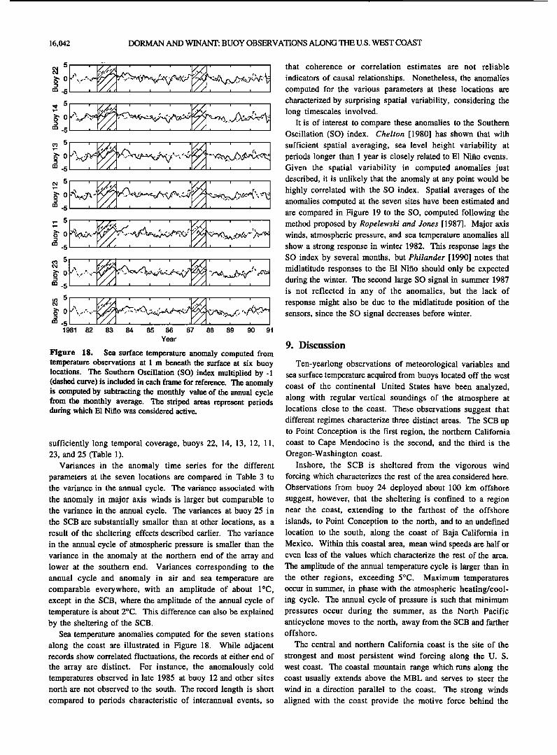
Figure 18. Sea surface temperature anomaly computed from temperature observations at 1 m beneath the surface at six buoy locations. The Southern Oscillation (SO) index multiplied by -1 (dashed curve) is included in each frame for reference. The anomaly is computed by subtracting the monthly value of the annual cycle from the monthly average. The striped areas represent periods during which El Nifio was considered active.

sufficiently long temporal coverage, buoys 22, 14, 13, 12, 11, 23, and 25 (Table 1).

Variances in the anomaly time series for the different parameters at the seven locations are compared in Table 3 to the variance in the annual cycle. The variance associated with the anomaly in major axis winds is larger but comparable to the variance in the annual cycle. The variances at buoy 25 in the SCB are substantially smaller than at other locations, as a result of the sheltering effects described earlier. The variance in the annual cycle of atmospheric pressure is smaller than the variance in the anomaly at the northern end of the array and lower at the southern end. Variances corresponding to the annual cycle and anomaly in air and sea temperature are comparable everywhere, with an amplitude of about IøC, except in the SCB, where the amplitude of the annual cycle of temperature is about 2øC. This difference can also be explained by the sheltering of the SCB.

Sea temperature anomalies computed for the seven stations along the coast are illustrated in Figure 18. While adjacent records show correlated fluctuations, the records at either end of

the array are distinct. For instance, the anomalously cold temperatures observed in late 1985 at buoy 12 and other sites north are not observed to the south. The record length is short compared to periods characteristic of interannual events, so

that coherence or correlation estimates are not reliable

indicators of causal relationships. Nonetheless, the anomalies computed for the various parameters at these locations are characterized by surprising spatial variability, considering the long timescales involved.

It is of interest to compare these anomalies to the Southern Oscillation (SO) index. Chelton [1980] has shown that with

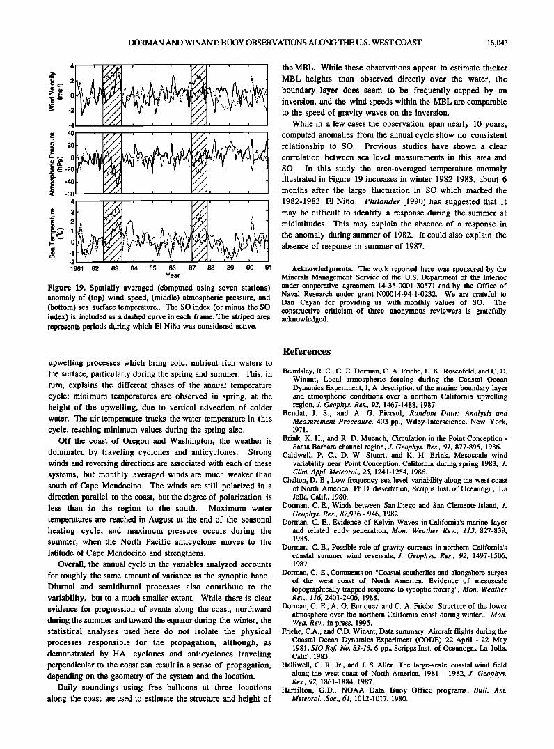
sufficient spatial averaging, sea level height variability at periods longer than 1 year is closely related to E1 Nifio events. Given the spatial variability in computed anomalies just described, it is unlikely that the anomaly at any point would be highly correlated with the SO index. Spatial averages of the anomalies computed at the seven sites have been estimated and are compared in Figure 19 to the SO, computed following the method proposed by Ropelewski and Jones [1987]. Major axis winds, atmospheric pressure, and sea temperature anomalies all show a strong response in winter 1982. This response lags the SO index by several months, but Philander [1990] notes that midlatitude responses to the E1 Nifio should only be expected during the winter. The second large SO signal in summer 1987 is not reflected in any of the anomalies, but the lack of response might also be due to the midlatitude position of the sensors, since the SO signal decreases before winter.

9. Discussion

Ten-yearlong observations of meteorological variables and sea surface temperature acquired from buoys located off the west coast of the continental United States have been analyzed, along with regular ve•'tical soundings of the atmosphere at locations close to the coast. These observations suggest that different regimes characterize three distinct areas. The SCB up to Point Conception is the first region, the northern California coast to Cape Mendocino is the second, and the third is the Oregon-Washington coast.

Inshore, the SCB is sheltered from the vigorous wind forcing which characterizes the rest of the area considered here. Observations from buoy 24 deployed about 100 km offshore suggest, however, that the sheltering is confined to a region near the coast, extending to the farthest of the offshore islands, to Point Conception to the north, and to an undefined location to the south, along the coast of Baja California in Mexico. Within this coastal area, mean wind speeds are half or even less of the values which characterize the rest of the area.

The amplitude of the annual temperature cycle is larger than in the other regions, exceeding 5øC. Maximum temperatures occur in summer, in phase with the atmospheric heating/cool- ing cycle. The annual cycle of pressure is such that minimum pressures occur during the summer, as the North Pacific anticyclone moves to the north, away from the SCB and farther offshore.

The central and northern California coast is the site of the

strongest and most persistent wind forcing along the U.S. west coast. The coastal mountain range which runs along the coast usually extends above the MBL and serves to steer the

wind in a direction parallel to the coast. The strong winds aligned with the coast provide the motive force behind the

DORMAN AND WINANT: BUOY OBSERVATIONS ALONG THE U.S. WEST COAST 16,043

'• •' '4 ••i , ' •, ,• . ; , , ' ,!'• > 0 • i' ,•;'/ ' ; '"

•'-' -2

• 20 • ,-,. ., E ß

• v

0

E • 60 ' ' '

4 .... •;.•, , , ;'"'""' "

m -1

-2 lg81 82 83 84 85 86 87 88 8g go gl

Year

Figure 19. Spatially averaged (domputed using seven stations) anomaly of (top) wind speed, (middle) atmospheric pressure, and (bottom) sea surface temperature.. The SO index (or minus the SO index) is included as a dashed curve in each frame. The striped area represents periods during which El Nifio was considered active.

the MBL. While these observations appear to estimate thicker MBL heights than observed directly over the water, the boundary layer does seem to be frequently capped by an inversion, and the wind speeds within the MBL are comparable to the speed of gravity waves on the inversion.

While in a few cases the observation span nearly 10 years, computed anomalies from the annual cycle show no consistent relationship to SO. Previous studies have shown a clear correlation between sea level measurements in this area and

SO. In this study the area-averaged temperature anomaly filustrated in Figure 19 increases in winter 1982-1983, about 6 months after the large fluctuation in SO which marked the 1982-1983 E1 Nifio. Philander [1990] has suggested that it may be difficult to identify a response during the summer at midlatitudes. This may explain the absence of a response in the anomaly during summer of 1982. It could also explain the absence of response in summer of 1987.

Acknowledgments. The work reported here was sponsored by the Minerals Management Service of the U.S. Department of the Interior under cooperative agreement 14-35-0001-30571 and by the Office of Naval Research under grant N00014-94-1-0232. We are grateful to Dan Cayan for providing us with monthly values of SO. The constructive criticism of three anonymous reviewers is gratefully acknowledged.

upwelling processes which bring cold, nutrient rich waters to the surface, particularly during the spring and summer. This, in turn, explains the different phases of the annual temperature cycle; minimum temperatures are observed in spring, at the height of the upwelling, due to vertical advection of colder water. The air temperature tracks the water temperature in this cycle, reaching minimum values during the spring also.

Off the coast of Oregon and Washington, the weather is dominated by traveling cyclones and anticyclones. Strong winds and reversing directions are associated with each of these systems, but monthly averaged winds are much weaker than south of Cape Mendocino. The winds are still polarized in a direction parallel to the coast, but the degree of polarization is less than in the region to the south. Maximum water temperatures are reached in August at the end of the seasonal heating cycle, and maximum pressure occms during the summer, when the North Pacific anticyclone moves to the latitude of Cape Mendocino and strengthens.

Overall, the annual cycle in the variables analyzed accounts for roughly the same amount of variance as the synoptic band. Diurnal and semidiurnal processes also contribute to the variability, but to a much smaller extent. While there is clear evidence for progression of events along the coast, northward during the summer and toward the equator during the winter, the statistical analyses used here do not isolate the physical processes responsible for the propagation, although, as demonstrated by HA, cyclones and anticyclones traveling perpendicular to the coast can result in a sense of propagation, depending on the geometry of the system and the location.

Daily soundings using free balloons at three locations along the coast are usexl to estimate the structure and height of

References

Beardsley, R. C., C. E. Dorman, C. A. Friehe, L. K. Rosenfeld, and C. D. Winant, Local atmospheric forcing during the Coastal Ocean Dynamics Experiment, I, A description of the marine boundary layer and atmospheric conditions over a northern California upwelling region, J. Geophys. Res., 92, 1467-1488, 1987.

Bendat, J. S., and A. G. Piersol, Random Data: Analysis and Measurement Procedure, 403 pp., Wiley-Interscience, New York, 1971.

Brink, K. H., and R. D. Muench, Circulation in the Point Conception - Santa Barbara channel region, J. Geophys. Res., 9], 877-895, 1986.

Caldwell, P. C., D. W. Stuart, and K. H. Brink, Mesoscale wind variability near Point Conception, California during spring 1983, J. Clim. Appl. Meteorol., 25, 1241-1254, 1986.

Chelton, D. B., Low frequency sea level variability along the west coast of North America, Ph.D. dissertation, Scripps Inst. of Oceanogr., La Jolla, Calif., 1980.

Dorman, C.E., Winds between San Diego and San Clemente Island, J. Geophys. Res., 87,936 - 946, 1982.

Dorman, C. E., Evidence of Kelvin Waves in California's marine layer and related eddy generation, Mon. Weather Rev., ]]3, 827-839, 1985.

Dorman, C. E., Possible role of gravity currents in northern California's coastal summer wind reversals, J. Geophys. Res., 92, 1497-1506, 1987.

Dorman, C. E., Comments on "Coastal southerlies and alongshore surges of the west coast of North America: Evidence of mesoscale

topographically trapped response to synoptic forcing", Mon. Weather Rev., ]]6, 2401-2406, 1988.

Dorman, C. E., A. G. Enriquez and C. A. Friehe, Structure of the lower atmosphere over the northern California coast during winter., Mon. Wea. Rev., in press, 1995.

Friehe, C.A., and C.D. Winant, Data summary: Aircraft flights during the Coastal Ocean Dynamics Experiment (CODE) 22 April - 22 May 1981, SIO Ref. No. 83-]3, 6 pp., Scripps Inst. of Oceanogr., La Jolla, Calif., 1983.

Halliwell, G. R., Jr., and J. S. Allen, The large-scale coastal wind field along the west coast of North America, 1981 - 1982, J. Geophys. Res., 92, 1861-1884, 1987.

Hamilton, G.D., NOAA Data Buoy Office programs, Bull. Am. Meteorol. .Soc., 6], 1012-1017, 1980.

16,044 DORMAN AND WINANT: BUOY OBSERVATIONS ALONG THE U.S. WEST COAST

Large, W.G., and S. Pond, Open ocean momentum flux measurements in moderate to strong winds, J. Phys. Oceanogr., 11, 324-336, 1981.

Limeburner, R. (Ed.), CODE-2: Moored array and large-scale data report, WHOI Tech. Rep. 85-35, CODE Tech. Rep. 38, 220 pp., Woods Hole Oceanogr. Inst., Woods Hole, Mass., 1985.

Mass, C.F., and M.D. Allbright, Coastal soutl',erlies and alongshore surges of the west coast of North America: Evidence of mesoscale topographically trapped response to synoptic forcing, Mon. Weather Rev., 115, 1707-1738, 1987.

Mass, C.F., and M.D. Allbright, Reply, Mon. Weather Rev., 116, 2407-2410, 1988.

National Oceanic and Atmospheric Administration, NDBC Data Availability Summarg, Nat. Data Buoy Cent. Rep. 1801-24-02, rev. G, 13 pp., U.S. Dept. of Commer., Washington, D.C., August 1992.

Neiburger, M., D. S. Johnson, and C. Chien, Studies of the structure of the atmosphere over the eastern Pacific Ocean in Summer, I, The inversion over the eastern North Pacific Ocean, Univ. Calif. Publ. Meteorol., 1, 1-94, 1961.

Nelson, C. S., Wind stress curl over the California current, NOAA Tech. Rep. NMFS SSRF- 714, 87 pp., 1977.

Overland, J.E., Scale analysis of marine winds in straits and along mountainous coasts, Mon. Weather Rev., 112, 2530-2534, 1984.

Panofsky, H.A., and J.A. Dutton, Atmospheric Turbulence, 397 pp., Wiley-Interscience, New York, 1984.

Philander, G., El Nino, La Nina and the Southern Oscillation, 293 pp., Academic, San Diego, Calif., 1990.

Reason, C. J. C., and D. G. Steyn, The dynamics of coastally trapped mesoscale ridges in the lower atmosphere, J. Atmos. Sci., 49, 1677-1692, 1992.

Ropelewski, C. F., and P. D. Jones, An extension of the Tahiti-Darwin southern oscillation index, Mon. Weather Rev., 115, 2161- 2165, 1987.

Samelson, R.M., Supercritical marine-layer flow along a smoothly varying coastline, J. Atmos.. Sci., 17, 1571-1584, 1992.

Strub, P. T., J. S. Allen, A. Huyer, R. L. Smith, and R. C. Beardsley, Seasonal cycles of currents, temperatures, winds and sea level over the northeast Pacific continental shelf: 35øN to 48øN, J. Geophys. Res., 92, 1507-1526, 1987.

U.S. Dept. of Commerce, NDBC Data Availability Summary, National Oceanic and Atmospheric Administration, National data Buoy Center Rept. No. 1801-24-02, rev. G, 133 pp., August 1992.

U.S. Navy, Climatological study of the southern California operating area, Nav. Weather Serv. Command, NWSED, Asheville, N.C., 1971.

Willebrand, J., Temporal and spatial scales of the wind field over the North Pacific and North Atlantic, J. Phys. Oceanogr., 8, 1080-1094, 1978.

Winant, C., C. Dorman, C. Friehe, and R. Beardsley, The marine layer off northern California: An example of supercritical channel flow, J. Atmos. Sci., 45, 3588-3605, 1988.

Zemba, J., and C. A. Friehe, The marine atmospheric boundary layer jet in the Coastal Ocean Dynamics Experiment, J. Geophys. Res., 92, 1489-1496, 1987.

C. E. Dorman and C. D. Winant, Center for Coastal Studies, 0209, Scripps Instititution of Oceanography, University of California, San Diego, La Jolla, CA 92093-0209. (e-mail: clive@coast.ucsd.edu; cdw @ coast.ucsd.edu)

(Received June 7, 1994; revised November 22, 1994; accepted November 28, 1994.)