VARIETY IN BUOY TECHNOLOGY AND DATA APPLICATIONS

PRESENTATIONS AT THE DBCP TECHNICAL WORKSHOP

(Marathon, Florida, October 1998)

INTERGOVERNMENTAL OCEANOGRAPHIC COMMISSION COF UNESCO)

OAT A BUOY CO-OPERATION PANEL

VARIETY IN BUOY TECHNOLOGY AND DATA APPLICATIONS

PRESENTATIONS AT THE DBCP TECHNICAL WORKSHOP

(Marathon, Florida, October 1998)

DBCP Technical Document No. 14

1999

WORLD METEOROLOGICAL ORGANIZATION

NOTES

The designations employed and the presentation of material in this publication do not imply the expression of any opinion whatsoever on the part of the Secretariats of the Intergovernmental Oceanographic Commission (of UNESCO), and the World Meteorological Organization concerning the legal status of any country, territory, city or area, or of its authorities, or concerning the delimitation of its frontiers or boundaries.

Editorial note: This publication is for the greater part an offset reproduction of typescripts submitted by the authors and has been produced without additional revision by the Secretariats.

FOREWORD

The success of technical workshops at the eleventh, twelfth and thirteenth sessions of the Data Buoy Cooperation Panel (DBCP) (respectively Pretoria, Henley-on-Thames and La Reunion, see DBCP Technical Publication No. 12) encouraged the panel to make such workshops a regular feature of its annual session, as a practical means of promoting cooperation and information exchange amongst all sections of the global buoy community, including buoy deployers, data users and communication systems providers.

Consequently, a technical workshop on Variety in buoy technology and data applications took place during the first day and a half of the fourteenth session of the panel, held in, Marathon, Florida, USA, in October 1998. Around 20 papers were read to more than 50 participants during the workshop, and the texts of 15 and abstracts of 4 of these are included in this DBCP technical publication. In all cases the papers have been reprinted as received, without additional editorial intervention.

TABLE OF CONTENTS

FOREWORD

TABLE OF CONTENTS

AGENDA

PRESENTATIONS

1. D.W. Jones and A.N. Bentley, UK Meteorological Office, United Kingdom Open-Ocean Data Buoy . . . . . . . . . . . . . . . . . . . . . . . . . . . . . . . . . . . . . . . . . . . . . . . . . . . . 1

2. Peter Thomas, Central Institute of Technology, New Zealand Issues Involved in the Design of an Autonomous Solar Electric Research Vessel for 9 Gathering Surface from Remote Areas ....................................... .

3. David B. Gilhousen, National Data Buoy Center, USA Dial-A Buoy Reaches Mariners . . . . . . . . . . . . . . . . . . . . . . . . . . . . . . . . . . . . . . . . . . . . . . 19

4. David Meldrum, Dunstaffnage Marine Laboratory, UK Recent Drifter Developments at Dunstaffnage: the Smart Buoy and the Mini Drifter . . . . 27

5. Mark Bushnell, NOAAIAOML-GDC, USA Recent Progress Using Orbcomm and Iridium for Drifting Buoy Data Transmission . . . . 31

6. Ngoc Huang and Jeff Wingwroth, TECHNOCEAN, NAL Research, USA Data Relay Systems for Drifting Buoys Utilizing Low-Earth Orbit Satellites . . . . . . . . . . . . . 33

7. Hal Brown, Ralph Cambre, Joel Chaffin and Charles Bond, National Data Buoy Center and Computer Sciences Corporation, Stennis Space Center, USA A Buoy-Mounted Air Traffic Control Radio Relay System . . . . . . . . . . . . . . . . . . . . . . . . . . 35

8. M. Blaseckie, S.G.P. Skey, K. Berger-North, J. Ploeg and PA. Bolduc, Axys Environmental Consulting Ltd., DFO/Canadian Coast Guard, Marine Environmental Data Service, Canada 41 The Cape Mudge Wave Experiments: Early Results ............................ .

9. David Wang and David Gilhousen, Computer Sciences Corporation and National Data Buoy Center, Stennis Space Center, USA Separation of Sea and Swell from NDBC Buoy Wave Data . . . . . . . . . . . . . . . . . . . . . . . . 53

10. Stephen E. Pazan and Peter P. Niiler, Ocean Prospects and Scripps Institution of Oceanography, USA Recovery of Near Surface Velocity from Undrogued Drifters . . . . . . . . . . . . . . . . . . . . . . . 61

11. John Stadler, Atlantic Oceanographic and Meteorological Laboratory, USA Development of a Drifting Buoy Metadata File at the Global Drifter Center . . . . . . . . . . . . 107

12. M. Taillade, CLS/Service Argos, France Preliminary Analysis of Argos 2 on NOAA K Perfonnances . . . . . . . . . . . . . . . . . . . . . . . . 109

13. Christine M. Caruso, National Oceanic and Atmospheric Administration, National Weather Service and National Centers for Environmental Prediction Central Operations, USA Interactive Real-time Quality Control of Surface Marine Data at the National Centers for Environmental Prediction . . . . . . . . . . . . . . . . . . . . . . . . . . . . . . . . . . . . . . . . . . . . . . . . . . . 123

14. Sveng-Aage Malmberg and Hedinn Valdimarsson, Marine Research Institute, Iceland Long Distance Drift from Icelandic Waters into the Labrador and Norwegian Seas 1995-1998 . . . . . . . . . . . . . . . . . . . . . . . . . . . . . . . . . . . . . . . . . . . . . . . . . . . . . . . . . . . . . . . . . . . . 131

15. Mark Swenson and Donald V. Hanson, National Oceanic and Atmospheric Administration/AOML, USA Mixed Layer Heat Budget in the Cold Tongue Region . . . . . . . . . . . . . . . . . . . . . . . . . . . . 133

16. David Cotton, Satellite Observing Systems, United Kingdom The Global Inter-Calibration of Satellite and Buoy Measurements of Winds and Waves . 135

17. D.W. Jones and H.M. Tanner, UK Meteorological Office, United Kingdom An Assessment of the Uncertainty in NWP Background Field Data Based on Duplicate Observations from Moored Buoys . . . . . . . . . . . . . . . . . . . . . . . . . . . . . . . . . . . . . . . . . . . . 143

18. Robert Molinari, Atlantic Oceanographic and Meteorological Laboratory, NOAA, USA Profiling-ALACE Floats in the Atlantic Circulation and Climate Experiment . . . . . . . . . . . . 155

19. H. Paul Freitag, Unda· J. Mangum, Nathan C.M. Franzen and Michael J.McPhaden, National Oceanic and Atmospheric Administration, Pacific Marine Environmental Laboratory, USA TAO Array Enhancements and Expansions ~ . . . . . . . . . . . . . . . . . . . . . . . . . . . . . . . . . . . 157

LIST OF PARTICIPANTS

AGENDA FOR SCIENTIFIC AND TECHNICAL WORKSHOP OF THE DATA BUOY COOPERATION PANEL

VENUE: Marathon, Florida DATE: October 12-13,1998

THEME: Variety in Buoy Technology and Appllcations

WORKSHOP CHAIR: Eric Meindl, National Data Buoy Center (NWS/NOAA), U.S.A.

Monday, October 12, 1998

Session I

Session II

Innovative Concepts in Moored and Drifting Buoy Design and Appllcatlon Chair- D. Wynn Jones, UK Meteorological Office, U.K.

Open-Ocean Data Buoy D. W. Jones and A. N. Bentley, United Kingdom Meteorological Office, U.K.

Issues Involved in the Design of an Autonomous Solar Electric Research Vessel for Gathering Surface Data from Remote Areas Peter Thomas, Central Institute of Technology, New Zealand

Dial-A-Buoy Reaches Mariners David B. Gilhousen, National Data Buoy Center (NWS/NOAA), U.S.A.

Recent Drifter Developments at Dunstaffnage: the Smart Buoy and the Mini Drifter David Meldrum, Dunstaffnage Marine Laboratory, Scotland- U.K.

Recent Progress Using Orbcomm and Iridium for Drifting Buoy Data Transmission Mark Bushnell, Atlantic Oceanographic and Meteorological Laboratory (OAR/NOAA), U.S.A.

Data Relay Systems for Drifting Buoys Utilizing Low-Earth Orbit Satellites Dr. Ngoc Huang (and Jeff Wingwroth, TECHNOCEAN), NAL Research, U.S.A.

An Air Traffic Control System Utilizing Moored Buoys Hal Brown, National Data Buoy Center (NWS/NOAA), U.S.A.

Applications of and Scientific Results Deriving from Buoy Data in Research or Operations Chair- Ellzabeth Horton, U.S. Naval Oceanographic Office, U.S.A.

The Cape Mudge Wave Experiment: Early Results M. Blaseckie, S.G.P Skey, K. Berger-North, J. Ploeg and P.A. Bolduc, Axys Environmental Consulting Ltd, DFO/Canadian Coast Guard, and Marine Environmental Data Service, Canada

Estimating Swell Information for NDBC's Web Site David Gilhousen and Dr. David Wang, National Data Buoy Center (NWS/NOAA) and Computer Sciences Corporation, U.S.A.

Recovery of Near Surface Velocity from Undrogued Drifters Dr. Stephen Pazan and Dr. Peter Niiler, Ocean Prospects and Scripps Institution of Oceanography, U.S.A.

Development of a Drifting Buoy Metadata File at the Global Drifter Center John Stadler, Atlantic Oceanographic and Meteorological Laboratory (OAR/NOAA), U.S.A.

Preliminary Analysis of Argos 2 on NOAA K Performances M. Taillade, Service Argos, Inc., France

Interactive Real-time Quality control of Surface Marine Data at the National Centers for Environmental Prediction Christine M. Caruso, NOAA/NWS/NCEP/Central Operations, U.S.A.

Long Distance Drift from Icelandic Waters into the Labrador and Norwegian Seas 1995-1998 Svend-Aage Malmberg and Heoinn Valdimarsson, Marine Research Institute, Reykjavik, Iceland

Mixed Layer Heat Budget in the Cold Tongue Region • Mark.Swanson and Donald V. Hanson

Tuesday, October 13, 1998

Sessionm Buoy Data as a Complement to Remote Sens~g, Modeling, and Other Discipllnes Chair- Ron McLaren, Environment Canada

The Global Inter Calibration of SateiUte and Buoy Measurements of Winds and Waves David Cotton, Southampton Oceanography Centre, U.K.

An Assessment of the Uncertainty in NWP Background Field Data Based on Duplicate Observations from Moored Buoys D. W. Jones and H. M. Tanner, United Kingdom Meteorological Office, U.K.

Profillng-ALACE Floats in the Atlantic Circulation and Climate Experiment Dr. Robert Molinari, Atlantic Oceanographic and Meteorological Laboratory (OAR/NOAA), U.S.A.

TAO Arr~y Enhancements and Expansions "Paul Freitag, Pacific ·Marine Environmental Laboratory (OAR/NOAA), U ~S.A .

• No written material submitted for the proceedings.

1. Abstract

- 1 -

OPEN-OCEAN DATA BUOY By D W Jones and A N Bentley

Based on many years operational experience, The UK Meteorological Office (Met Office) has developed an Open-ocean Meteorological Data Buoy capable of continuous extended operation in the severe environment of the north-east Atlantic Ocean. The buoys are equipped with duplicated sensors and data collection systems. Each buoy also has two Meteosat DCP transmission systems, each of which transmits both sets of collected data every hour. This redundancy significantly reduces the potential for data loss due to any sensor failure, or failure of either of the data collection or transmission systems. The duplicate data sets also enable quality control and selection of the ' best' before coding and dissemination on the GTS. The paper includes a description of the main design features, the sensors and data acquisition systems. It also describes some of the enhancements, to both the buoys and the network, planned for implementation within the next year.

2. Introduction

IQ

' tUM

Sole

KEY:

.,. · Shipping arus

- 'f Moored buoya

• Platf- Md btad• 1 UShtshlp'

Figure 1 UK Met Office (UKMO) Network of Marine Automatic Weather Stations

Figure 1 shows the UK Met Office (UKMO) network of manne automatic weather stations and their associated World Meteorological Organisation (WMO) numbers.

This paper describes the moored buoy part of this network with particular reference to the open­ocean buoy design which is used at all buoy stations except Lyme Bay, Aberporth and Luce Bay.

The buoys are also in use at the Brittany and Gascogne Stations as collaborative projects with Meteo France.

- 2 -

3. The Open-Ocean and Inshore Buoys

' • !

Figure 2 Inshore Design

Figure 3 Open Ocean Buoy

Figures 2 and 3 show the UKMO lnsho:r;e and Open­Ocean Buoys.

The inShore design {figure 2) is a 2..5 metre diameter toroidal buoy using a singie electronics payload and sensor suite with .a UHF, line-of-site, communications link to a local shore station. These buoys are generally deployed in relatively shallow waters, up to 50 metres and have the advantage that in addition to providing automatic hourly reports they can also be interrogated.

The open-ocean buoy (Figure 3) has been designed to operate in virtually any water depth from 30 metres to 6,000 metres, in all sea conditions, at least all those encountered in the North- Eastern Atlantic.

It has a hull diameter of 2.8 metres, an overall height of 6.0 metres and it weights 4. 1 tonnes, in its operational state.

Buoyancy is provided by a closed cell foam floatation collar protected by self-coloured elastomer skin approximately 10 mm thick. The total reserve buoyancy of the buoy is 5 tonnes which enables it to carry the entire mooring system without being submerged, for example, if the buoy is dragged out of its mooring depth. The hull has a cylindrical steel foot, which allows it to be free standing when out of the water, and fins which reduce rotational motion when it is at sea.

- 3 -

The superstructure is 3.0 metres high and manufactured from marine grade stainless steel; it is free standing when separated from the hull. It incorporates a single point lifting eye and is stressed to safely take the weight of the buoy and mooring during deployment and recovery. The superstructure incorporates a 'crow' s nest' arrangement with a 1.5 metre diameter ring at its top, made from 1 inch stainless steel tube, on which wind sensors and antennae are mounted; this is 4 metres above nominal sea level when deployed. There are also lower bars for the mounting of barometric pressure, air temperature and humidity sensor housings.

The sensors and antennae are mounted by means of quick release clamps which are easy to operate in rough sea conditions and without the use of special tools. The superstructure also incorporates access ladders, solar panels, radar reflectors, and a single navagation lamp to meet the safety provision of ODAS Aids and Devices published by the Inter-Governmental Marine Consultative Organisation (IlviCO).

In addition to the meteorological and oceanographic variables the buoys also report location using the GPS, plus house keeping data such as electronics supply voltage, electronics pod humidity and temperature, navigation lamp status, battery charge and discharge currents, transmission count and hull dry or flooded.

4. Sensors

All sensors, except the wave sensor, are duplicated and all except the wave and sea temperature are mounted externally and can be exchanged at sea. The variables reported and sensor types are given in Table 1. All sensors are calibrated at the UKMO test and calibration facility, before being used operationally. This includes a purpose built, vertical, wave sensor calibration rig which is capable of simulating sinusoidal and complex waves of up to 4 metres peak to trough and periods in the range 3 to 30 seconds. Check observations are also taken on station before and after sensors are exchanged.

Variable Reported Value SeusorTvue

Wind Speed The ten minute average preceding the observation time Rotating cup anemometer.

Maximum Gust The maximum 3 second value since the last synoptic Rotating cup anemometer. observation.

Wmd Direction Averaged as for wind speed Self referencing wind vane.

Barometric A ten second average not colTected to mean sea l~'lel. Aneroid capsule or vibrating cylinder. Pressure

Relative Humidity An instantaneous value. taken at the observation time. Electrical conductors set in a wafer of a chemically treated styrene copolymer with an integral non conducting substrate. Protected against salt water contamination.

Air Temperature A ten second average. Platinum resistance thermometer in an ODAS radiation screen.

Sea Surface A ten second average at a nominal depth of 1 metre:. Platinum resistance thermometer mounted in a hull Temperature contact housing.

Significant Wave 4 x RMS value of the wave hc:ight, and the aveDge An accelerometer the output of which is doubl~ Height and Wave crossing interval of the wave through the mean watc:r integrated to produce hc:ave.

Period levc:I. for 17.5 minutes preceding th~ observation time.

Table 1 Variable, Reported Value and Sensor Type

- 4 -

5. The Electronics Payload

A schematic diagram of the open-ocean buoy electronics system can be seen at Figure 4. It is fully duplicated, with the exception of the wave sensor, with crossover interconnections for increased system integrity whenever possible.

'WINO DUEcnOH 'WIN0Sf£ED AIR TEMP SEA TEMP KJMili1Y FRESSUI'I:

B.£CJAONICS MIMDTY DM.I+t2V NAVUOHT MOHJTOR A.O REFERI:NCE HUU. FLOODED SYSTEM almi:N1' (HOIRYTOTAI.)

~

W!HDDCRECnOH WIHDSf'EED AIR TEMP SEA TEMP KJMDTY FRESSUfE

. B.ECffiONICS KJMili1Y IWI+12V NAVUOHT

· MONITOR M) f8'ERENCE HUU.R.OOCIED SY5TEit aJmi:N1' eta.RYTOW.)

DA~

~TA CONBlHER

11

ACQUISITION pCIOIFUTER

~8'lllfl~ullDI~' P!!:::VI u: J======~ n (CR10)

Figure 4 Schematic Diagram

Each data acquisition system is based upon a PC programmable, proprietary data logger, The CRIO, manufactured by Campbell Scientific. The logger output is then converted to a unique marine automatic weather station (MAWS) code, within a programmable·, single board microcomputer, which takes in position data directly from the GPS.

The data from each of the two microcomputers are then united within two data combiners, the outputs of both combiners are then passed to two DCP satellite transmitters. Consequently each transmission contains data from both suites of sensors and both data acquisition systems.

The power output of the DCP transmitter is 25 Watts. This has proved to be sufficient to ensure reliable operations for latitudes up to at least 60°. To ensure timely availability of the data, both for NWP models and forecasters, DCP transmission slots between HH-8 and HH +10 have been selected. Data are received at the ESOC reception facility at Darmstadt from where they are forwarded to the UKMO Communications Centre at Bracknell, for data selection and recoding into WMO FM13 Ship Code for retransmission on ·the Global Telecommunications System (GTS).

- 5 -

6. Location

Being moored, the nominal location of the buoy is known, at least within the circle of movement which results from the inverse catenary mooring (see Section 10). However the activities of fishing boats and other unwarranted interference does occasionally result in buoys going adrift Consequently two Global Positioning System (GPS) receivers are installed on the buoy and the location data are included in the transmitted message. As a backup, in the event of a buoy suffering major damage to the superstructure, an Argos PTI, with an independent power supply, is incorporated into the hatch cover of the hull.

7. Power Supply

Each of the two independent sensor and electronic systems on the buoy have their own battery packs, each charged by two solar panels, one on each side of the superstructure. In the unlikely event of the total failure of the solar charging system, a fully charged set of the lead acid gel batteries have sufficient capacity to power the buoy for at least three months. Even at 60° north the solar panels supply sufficient charge to maintain the buoy throughout the winter.

8. The servicing of Open-Ocean Buoy stations

The present practice is for a servicing visit to each station every six months for a routine change of external sensors. The upper moorings are inspected every 12 months and the complete buoy is exchanged every two years. The mooring is changed at three yearly intervals.

9. Data

9.1. Data Coding

Under nonnal circumstances, four sets of observational data are available every hour (two transmissions each containing data from both sets of sensors) at the UKMO Communications Centre. Clearly only one set of data is needed to compile an observation and so a selective process has to be implemented. Nonnally the FM13 coded observations are made from sensor suite 1 data via transmission 1. However, if the transmitter or data acquisition system or individual sensors in the sensor suite fail, the FM13 message is compiled from the best available data.

9.2. Data Quality Control

In addition to reducing the potential data loss due to sensor failure, the duplication of sensors provide an opportunity to compare data, and thereby give enhanced confidence in the data quality. There are three levels of quality control used at present:

- 6 -

• WMO FM13 Synoptic Observations are routinely compared against data from the Background Field by the Met Office Quality Evaluation Section. In addition to identifying individual gross errors their process also produces monthly statistics of biases and variances.

• Snapshot checks of the meteorological and oceanographic data are undertaken daily by internal comparison of the duplicated sensor data. Any anomalies are checked immediately against synoptic charts and/or background fields and, if appropriate, changes to the preferred sensor data are made. These daily checks also include monitoring of buoy location and the engineering housekeeping data.

• Data received at UKMO Marine Operations facility, via a Meteosat Retransmission Link, enable the duplicated data to be checked for individual observations and graphically as a time series.

10. The Mooring

In water depths of 30 to 100 metres an all chain mooring is used, with a sub-surface float where appropriate.

The mooring used in deeper water is an inverse catenery type (see Figure 5) with a.1 tonne reserve buoyancy sub-surface float Moorings based on this principle are in widespread use by, for example, the NDBC and Environment Canada. The principle difference with the UKMO design is the use of a 1 tonne reserve buoyancy sub- surface float and an acoustic release; although the continued use of these is currently under review .

11. The Future

As with all operational programmes, enhancements aimed at improving the perfonn~ce and/or the cost effectiveness are continually being sought Developments now on trial are:-

• An alternative digital pressure sensor offering high accuracy and long term stability at much reduced cost.

• An improved static pressure head with a Goretex filter, to prevent water ingress, similar to that used on the WOCE drifting buoys.

• An active radar enhancer.

• A solid state wave sensor based on multiple accelerometer and tilt sensors. In addition to significant wave height. This will provide spectral and wave direction data, is a much smaller unit than the Datawell Heave Meter, presently in use, and if successful will permit the use of duplicate wave sensors.

• An Acoustic Doppler Current Pro tiler (ADCP).

- 7 -

12. Conclusion

14

13 12

11

The Met Office Open-Ocean Buoy is a successful design, having proved itself over many years as capable of providing reliable observations in the severe conditions encountered in the Northeast Atlantic. To date however, the buoys have been deployed to meet a meteorological operational requirements but as components of a long term operational programme they offer an opportunity to be developed as platforms for other oceanographic and environmental measurements.

18

13

17 1&

18

1&

14

15

8

10

0

E: SPLICE

~~ SEABED

t=·

MOORING DEPTH UP TO 6000m

MATERIALS ;:--;-'i'ONNE IRON SINKER OR EQUIVALENT

2. 3anm ANCHOR SHACKLE CLENCH

3. 38l1lm OEL X 27.&n

4. 3anm .JOINING SHACKLE CLENCH

&. ACOUSTIC RI!LEASE WITH RELEASE RING

8. 3anm BOX SWIVEL

7. 4Bmm 8 STRAND MULTIPLAIT POLVOLEOFIN PENDANT

8. GALVANISED THIMBLE AND LINK ASSEMBLY

o. 38l1lm BOX SWIVEL

10. SUB SURFACE FLOAT (MAXIMUM WORI<INQ DEPTH 1.5Km • RESERVE BUOYANCY 1 TONNE)

11. PENDANT x 1211m COMPRISINQ 4Bmm 8 STRAND NYLON MULTPLAIT x 1135m SPLICED INT04enm 8 STRANO MULIPLAIT POL'f'OLEOFIN X 138m

12. GALVANISED TUBULAR THIMBl..E (PROTECTED BY POLYURETHANE ENCAPSULATION) AND LINK ASSEMBlY

13. 2&mm ANCHOR SHACKLE CLENCH

14. 2&nm0Elx27.&n

15. 25mm .JOINIHG SHACKLE CLENCH

Ul. 2&nm BOX SWIVEL

17. 2&nm OELx 2m

18. OATABUCW

.!:!2!!':·

QTY --,-1

2 OR MORE (SEE NOTE 4)

5 OR MORE (SEE NOTE 4)

1 OR MORE (SEE NOTE 2)

3 OR MORE (SEE NOTES 2 6 3)

1 (SEE NOTE 5)

2

2

3

1. ALL STEELWORK IN THE t.IIOORINQ SHALL BE FORGED STEEL MANUFACTURED IN ACCORDANCE WITH ISO 1704 (1073) AND BS 070 EN14A

2. THE LENQTH OF ITEM7 IS 11001n FOR A MOORING DEPTH OF 2000m.IF THE MOORING DEPTH IS INCREASED AOOtTlONAL ITEM rs OF 11001n OR LESS, WITH APPROPRIATE NUMBER'S OF ITEM a, SHALL BE USED AS REOUIRI!O.

3. POL'f'OLEOFIN TO BE PROTECTED BY CANVAS OR NYLON SERVING /IJ ITEM 8 Cc::INIIECTIONS.

4. FOR MOORlNG DEPTHS GREATER THAN 200Cim. EXTRA ITEM'S 3 AND 4 MAYBE RI!QU!REO TO COMPENS/IJE FOR THE BUOYANCY OF THE EXTRA ITEM 7'8.

5. ITEM10 HAS THROUGH STEEL WITH 2& TONNE SWl. PAD EYES AT EACH END.

lilT 4 3 2 1

Figure 5 Inverse C&tenery Type Mooring

- 9 -

ISSUES INVOLVED IN THE DESIGN OF AN AUTONOMOUS SOLAR ELECTRIC RESEARCH VESSEL FOR GATHERING SURFACE DATA FROM REMOTE AREAS.

AUTHOR: PETER THOMAS

ABSTRACT

This paper outlines the major parameters involved in the design of the

smallest conceivable autonomous solar electric research vessel capable of

staying at sea for long periods. The design considerations are broken down

into three main interrelated areas. These are: Hull Design, Navigation,

Energy Management and Propulsion.

During this decade a· number of technical innovations have matured to make it possible

to produce an unmanned research vessel, powered by photo voltaic cells.

The specification for these unmanned vessels requires them to be capable of leaving their

home port under their own power, navigating to a required destination, maintaining

station at that location and eventually returning to their home port for a refit.

During their period at sea they radio back the data which they have gathered.

This paper discusses the issues involved in the design of the smallest conceivable vessel

capable of performing these tasks. It is concerned only with the vessel as an ocean going

research platform, it does not consider what instrumentation research workers may wish

to install in it.

The problems involved can be divided into three (interrelated) areas. These are:

1. Hull design

2.

3.

Navigation

Energy Management and Propulsion

- 10 -

Hull Design

Initial calculations showed a vessel4 metres (13 feet) long should be capable of converting

enough solar energy into electricity to b~ capable of powering itself over long periods. The

vessel needs to be self righting under all conditions (this requirement ruled out the use of

multihulls ). If about Y3 of the vessel's weight were to be dedicated to sealed deep cycle

lead acid batteries, the vessel would be able to run through the night by consuming the

surplus energy generated the previous day.

The positioning of the solar panel became a critical part of the hull design. The panels

form an inverted V over the hull, with the angle of the apex 90°. There are a number of

reasons for this.

1. More solar energy can be obtained when the sun is low in the sky.

2. The volume of air enclosed by the solar panels enables the vessel to meet its self

righting requirements.

3. The steepness of the sides facilitates rapid salt water run off and does not allow the

water to evaporate from the surface of the panels leaving behind pools of salt.

4. The slope is too steep and slippery-for sea birds to stand on and foul the panels.

5. Wind striking the surface of the 45° panel produces equal capsizing and righting

moments.

Keeping the vessel as small and low cost as possible means the energy equations for the

vessel are tight. Most of the energy consumed by the vessel is consumed by the propulsion

system. As a result the hull needs to be as efficient as we can make it.

The wetted surface has been reduced to a minimum by making the vessel round bilged.

This reduced the frictional resistance to a minimum. Optimum prismatic coefficient and

almost ideal angle of entry reduce the wave making losses as far as possible. There will be

days when heavy cloud cover results in significantly reduced solar electric generation.

- 11 -

When this happens it is advisable to prevent the vessel drifting too far off course. This is

achieved by a special rudder design.

The rudder is made in two halves. (Rather like a book). Under normal operation the

rudder is turned as a book would be turned about its spine.

If the boat is required to maintain station the two halves of the rudder open up (like a

book opening up) and the rudder acts as a drogue. When the drogue facility is no longer

required two halves of the rudder close and the rudder operates normally.

The vessel is powered by a single permanent magnet brushed DC motor with direct drive

via a maganese bronze log tube. The log tube is part of a single casting incorporating a

bronze skeg and the sea water inlets for the cutlass bearing and the bottom bearing for

rudder.

- 12 -

Navigation

The vessel is self guided not radio controlled.

The required route is pre programmed into the GPS with all appropriate waypoints. The

bearing to the next waypoint is calculated. This is the magnetic bearing and the boat takes

into account variation due to the fact the magnetic poles are different from the true poles.

The vessel uses a fluxgate (electronic) compass to determine the vessel's magnetic bearing.

The compass takes into account the vessel magnetic deviation. So the bearings are

magnetic bearings with both variation and deviation corrections made. Drift is also taken

care of as the GPS recognises only the course over the ground, not the course through the

water.

In addition to steering towards the next waypoint, the vessel also considers the cross track

error (which is integral control). This cross track error is included to get the vessel rapidly

back on course should it have been driven off course by adverse weather conditions.

Should the vessel temporarily lose satellite coverage, the magnetic bearing to the next

waypoint is stored in memory and the vessel continues to steer on its existing course until

satellite coverage returns.

The steering servo system takes into account the fact that larger rudder movements are

required when the vessel is moving slowly through the water than when the vessel's water

speed is high. It does this by changing the gain of the servo system. If this was not done,

the vessel would be underdamped at high speeds and overdamped at low speeds.

- 13 -

Energy Management and Propulsion

Most of the energy consumed by the boat is used for propulsion. This provides a method

of controlling energy consumption. The amount of electrical energy produced by the photo

voltaic cells is weather dependent. The vessel carries sealed deep cycle lead acid batteries,

which account for about % of the vessel's weight. This provides enough battery storage

for the boat to run through the night. The weight of the batteries significantly lowers the

centre of gravity of the boat to make it self righting under all conditions.

The vessel contains two battery systems. There is a 24 volt system and a 12 volt system.

The 24 volt system runs everything on the boat. The output of this battery supplies the

power for a 10 kHz 1 OOV AC regulated sinusoidal supply. This supply uses class C push

pull amplification running in parallel resonance. AC power is then reticulated round the

vessel and each electrical system has its own ferrite transformer and rectifier. This

provides electrical isolation between systems. In most cases, further DC analogue

regulation is not required because the AC supply is already regulated. Also as it is run in

parallel resonance which is fed from an above resonance series resonant circuit, the system

is short circuit (and student) proof, thus eliminating the need for additional fault protection.

It has a very high efficiency. The PWM supply for the main motor drive however runs

directly from the 24 volt battery system. This is fitted with electronic over current

limitation.

The 12 volt system normally does nothing. This is the uninterruptiable power supply

(UPS) which will maintain all essential services should adverse weather conditions result

in failure of the 24 volt system. The essential services do not include the propulsion

system and, without the main motor running, there is no point in running the steering

system servo. However, services like the radio, energy management system. GPS,

navigation lights, will run for weeks if necessary, even if the vessel were to obtain no solar

energy at all.

- 14 -

The vessel carries six nitride treated, laser grooved monocrystaline silicon solar panels.

Four panels are dedicated to the 24 volt system and two are dedicated to the 12 volt

UPS system. Under normal circumstances the UPS cattery will be fully charged on

standby. In this situation the surplus energy from the two UPS solar panels is diverted

into the 24 volt system. So the usual situation is to have a fully charged 12 volt UPS

system and all six solar panels feeding the 24 volt system which supplies all the vessel's

power.

The solar panels are fitted with auto tracking electronics. This ensures the panels are

always running at maximum theoretical efficiency. For example a 36 cell solar panel may

·deliver maximum power when its output is 18 volts and say 5 amps (90w). Ifthis solar

panel were to be fed into a 12 volt battery the panel would still deliver only 5 amps but

with a terminal voltage of 12 volts (60w) (current flowing is proportional to the number

of photons striking the panels).

·unfortunately the nominal 18 volt panel output and the nominal battery terminal voltage

are both variables. The vessel's auto tracking system ensures the panel is always running

at· max power output regardless ofthe panel and battery voltage. It is always tuned to

peak power.

The· vessel has. two energy management. systems. One .system predicts how much energy

should be available taking into account the latitude and longitude of the vessel, the

vessel's course, the date and time. It· assumes clear conditions and predicts how much

energy should be available taking into account the air mass (the path length the sun's

rays take through the atmosphere). The vessel measures how much energy it is receiving

and compares this with the theoretical maximum. It then pre~umes this ratio of actual to

optimum will continue until dusk. The programme continuously updates. From this

ratio the vessel works out how much power it should be using so that it will not run out

of energy before the next dawn.

In addition to this the vessel has a hardware back up system. This takes control initially,

when the boat is first turned on, and remains in control until one hour after the next

- 15 -

dawn. Or it takes control if the vessel has an energy management crisis, ie. the main 24

volt battery system is either running flat or is getting overcharged. In which case, it

provides rapid response to the crisis. It determines the degree of severity of the problem.

It contains a self learning system so that the average values it proposes are based on what

happened yesterday, which in turn was a response to what happened the day before, and so

on. In this way it adjusts to changing latitudes and changing seasons.

- 16 -

SOLAR BOAT SPECIFICATIONS

Mechanical specifications

Name:

Length (LOA):

Length water line (LWL):

Beam:

Self righting:.

Draft:

Displacement:

Hull material:

Antifouling coating:

Maximum speed:

Cruising speed:

Motive power:

Solar Electric Research Vessel "GOODWILL"

4.0 metres (13 feet)

3.85 metres

0.860 metres

All positions

340mm

200Kgs

Fibre reinforced plastic

Copper within the gel coat

5.5 knots (II Kmlhr)

4 knots (8 Kmlhr)

Electricity

- 17 -

SOLAR BOAT SPECIFICATIONS

Electrical specifications

Motor:

Maximum power:

Cruising power:

Number of solar cells:

Total area of solar panels:

Maximum power generated per panel:

Electrical storage:

Power reticulation:

24 Volt DC, permanent magnet

280 watts

100 watts

6 monocrystaline laser grooved silicon panels

3.8 sq. metres

85 watts

3 x 65 Ah 12 volt sealed deep cycle lead acid batteries

100v AC 10kHz

- 18 -

SOLAR BOAT

On board systems

• Primary energy management (software)

• Backup energy management electronics

• Battery charging and monitoring electronics

• Global positioning system (Garmin GPS45 Personal Navigator)

• Fluxgate compass (Azimuth 1000 Digital Compass)

• Satellite radio (Argos satellite system for tracking and communicating with the boat)

• Bilge pump electronics

• Navigation light and drogue motorelectronics

• Main motor electronics

• Steering motor electronics

• Microcontroller network

• 1 OOv 1OOKHz AC inverter

- 19 -

DATA

How to Hear Our Observations on the Phone

How Does Dial-A-Buoy

Work'!

What Should I Dolt' ... ?

What is Dial - A-Buoy?

Mariners can now hear the latest coas tal a nd offshore weather observations t hrough a new telephone service called Dial-A-Buoy. Dial-A-Buoy provides wind and wave measurements taken within t he last hour at 65 buoy and 54 Coastal- Marine Automated Network (C-MAN) stations . The stations are located in the Atlantic, Paci fi c , Gulf of Mexico , and t he Grea t Lakes and are operated by the National Data Buoy Center (NDBC). NDBC, a part of the National Weather Service (NWS) , created Dial-A-Buoy to give mariners an eas y way to obtain the report s via a cell phone.

Large numbers of boaters use the observatio ns , in combination with forecasts , to make decisions on whether it i s sa fe to ventu r e out. Some even claim t hat t he reports have saved lives. Surfers use the reports to see if wave conditions are, or will soon be, promising . Many of these boaters and surfers live well inland, and knowing the conditions has saved them many wasted trips to the coast .

An i ncreasingly popular way to obtain the observations has been through the Internet . In fact , NDBC ' s web site has received

- 20 -

more than a million hits a month. "Dial-A-Buoy is a logical extension to the Internet," states NDBC's David Gilhousen. "It will allow the mariner a way to get the conditions while offshore, at the marina, or away from the Internet.~

Buoy reports include wind direction, speed, gust, significant wave height, swell and wind-wave heights and periods, air temperature,. water temperature,. and sea level pressure. Some buoys report wave directions. All C-MAN stations report the winds, air temperature, and pressure; some also report wave information, water temperature, visibility, and dew point.

How do I use DiaL-A-Buoy? To access Dial-A-Buoy, dial (228} 688-1948 using any touch tone or cell phone. Assuming you know the identifier of the station whose report you need, enter 1. Then, enter the five-digit (or character) station identifier, followed by the # sign, in response to the prompt. The s.ystem will ask you. to confirm that your entry was correct by pressing 1. After a few seconds, you will hear the. latest buoy or C-MAN observation read. via computer­generated voice. Characters are entered simply by pressing the key containing the character. For Q, press "7~F and for z~ presses "'9·". Please be patient and wait for the system to finish prompting you; Dial-A~Buoy will not understand your entry if you are too fast.

Dial-A-Buoy also can read the latest NWS marine forecast for most station locations. If this option is available, the system will prompt you to press the i key after the obs.ervation is read. Wait to hear the· tone at the end of the prompt before pressing the # key.

When you are finished with Dia~-A-Buoy, simply hang-up!

There are several ways to find the station locations and identifiers. For Internet usersr .maps showing buoy locations are given at http: //www.ndbc •. noaa.gov/ .. Telephone users have several options·.. . They can enter a fa·x.. number to. receive. a location map by following the prompts. Or, they can enter a latitude and longitude and receive the closest station locations and identifiers.

How Does Dia.l-A-~oy Work? The Dial-A-Buoy system does not actually dial into a buoy or C-MAN station. The phone calls are answered by a computer at the Stennis Space Center iri Mississippi, where NDBC is located. The computer runs Web-on-Call software to control the dia·log and read the forecasts and observations from NDBC's web site. Web-on-Call, a commercial product from.General Magic Corporation of Sunnyvale, California, controls the reading of Web pages over the phone ..

Dial-A-Buoy is a proof-of-concept system that seeks involvement from the private sector. The eight-line system could be expanded through sponsorship by a private corporation such as a boating or meteorological organization. Alternatively, these organizations could offer a similar service at another location. This could easily be accomplished by running Web-on-Call software that would obtain the observations from NDBC's web site.

What are some prob1ems with Dia1-A-Buoy?

Dial-a-Buoy Introduction - 21 -

I entered a station identifier, but heard a response "Sorry, I did not recognize that selection. " You entered the station identifier too soon . Wait until the system finishes asking you for the identifier .

How do I enter characters for a Station Identifier? Characters are entered simply by pressing the key containing the character . For Q, press "7 ", and for Z, presses " 9" . For example, to enter CHLV2 , press the keys 24582 followed by the # sign .

I entered a valid station identifier, but heard a response saying that the topic was unavailabl e after about 6 second delay. Occasionally, the Internet ge ts very busy here at Stennis Space Center . The Web- On-Call software, which runs Dial- A- Buoy, has been programmed to give this response if it cannot obtain our web page to read in about 5 seconds . So , unfortunately, the answer is : Try again later .

I pressed the pound sign to get a marine forecast but heard the response , " Sorry I did not recognize that selection . " You entered the pound sign too early . Wait until you hear a tone to press the pound sign. How do I quit Dial-A-Buoy? Simply hang - up . Ho w do I hear the observations for another station? When you are finished hearing the observations or forecasts , the system will begin a long prompt saying , "To listen to this topic again, press 1 ..... . " If you press 6 at this point , Dial - A- Buoy will take you back to the beginning of the dialog .

This page was last modified on Monday, 10-Aug-98 12:53:20 CDT

_.,,.,' J=----• "/:")IIJ:J :•o:·---''J1"'''f :Jftl ''·--'"'••:l:•o•'•'•''--?"'"r-r ...11'_::"_ J #• .. ,.:,.11 • .,., • ' ~ ' "-I .. J;J . . J)J•. .... "__» :. I

Home I Webmaster I Disclaimer I Guest Book I FAQ

NDBC'S DIAL-A-BUOY SYSTEM

COMPUTER VOICE RESPONSE SYSTEM THAT

• READS LATEST OBSERVATION

- COASTAL-MARINE FORECASTS - CLOSEST STATIONS GIVEN POSITION

• FAXES STATION LOCATION MAPS

98-054(2)

N N

DIAL-A-BUOY SYSTEM

1. ENTERS STATION

4. READS PAGE 0 8 PENTIUM PC

WEB-ON-CALL SOFTWARE

5. OPTIONAL FAX

2. REQUESTS PAGE

3. OBTAINS DATAl ~ ITIJ I: :~I

D

OF STATION MAPS

WEB SERVER

98-054(2)

1\.)

w

DIAL-A-BUOY REACTION

• AVERAGES 700 CALLS A DAY

• REACHES MANY WHO CANNOT TRAVEL IN CYBERSPACE

• ONE USER COMMENT: "DIAL-A-BUOY IS A GREAT IDEA! AND "COOL" TOO. I ·,

WILL BE SURE TO TELL THE WIND-SURFING CROWD ABOUT IT • •• IT IS GREAt TO SEE··A TRUL.Y USEFUL EXPENDITURE OF tAX DOLLARS." . . . . . .

• PAIVATE SECTOR INTEREST: NEW JERSEY COMPANY TO START 1•900 NUMBER BOAT iUS INTER.ESTED IN OFFERING SERVICE IN: SELECTED AREAS

• l ,... r '' • · • '

! .

98-062(1)

1\J ~

WEB-ON-CALL, VERSION 2 IMPROVEMENTS

• USERS CAN ENTER STATION IDENTIFIER BEFORE THE PROMPT HAS FINISHED

• SYSTEM QUICKLY RECOGNIZES LINES WHERE THE USER HAS HUNG UP TO GIVE GREATER CAPACITY

• NDBC CAN TAILOR THE PROMPT AT THE END ALLOWING USERS TO EASILY REQUEST A SECOND STATION

• SYSTEM WILL ALLOW NDBC TO INCREASE THE TIME THAT WEB-ON-CALL WILL WAIT FOR A STATION PAGE TO BE OBTAINED FROM THE NDBC WEB SITE

98·062(1)

tv Ul

- 27 -

Recent Drifter Developments at Dunstaffnage: the Smart Buoy and the Mini Drifter

David Meldrum Centre for Coastal and Marine Sciences

Dunstaffhage Marine Laboratory Oban PA37 IQA

Scotland

INTRODUCTION

The increasing military requirement for rapid environmental assessment (REA} has stimulated the development of a number of expendable oceanographic sensor systems. At Dunstaffnage we have developed a 'smart' drifter for REA which evaluates the data from its sensor suite (thermistor string plus GPS receiver), according to user-specified criteria, and only transmits profiles which it considers will be of interest to the user. Currently, Argos is used as the communications channel. Satellite over-passes are predicted by the on board processor and data uploads scheduled accordingly. This approach optimises data transfer and minimises the risk of detection.

In a separate development, a mini-drifter has been produced for near-shore studies. Bi-directional UHF telemetry is used to receive DGPS corrections from a shore station. Corrected DGPS locations are broadcast over the return link and displayed in real time on a navigation chart using commercially available ship navigation software. The drifter has been used to study pollution trajectories close to fish farms.

THE ADAPTIVE SAMPLING 'SMART' TZ BUOY

Adaptive Sampling

A basic belief in oceanography is that the oceans contain too much data for the entirety to be measured, recorded and processed in any simple-minded fashion. This is particularly true if the goals of operational ocean observation in support of climate modelling and prediction are to be realised cost-effectively. Even if enough ocean platforms (moored instruments and buoys, drifters, profilers, autonomous submersibles, ships) could be deployed to make measurements at the required accuracy and density, the data communications and processing burden would be overwhelming. Furthermore, much of these data would be uninteresting and of little or no impact on the analysis, and would only serve to consume valuable energy, communications bandwidth and data processing resources. The costs of this profligacy are even more damaging in the military case of 'Rapid Environmental Assessment' (REA), where unnecessary data transmissions increase the risk of detection and countermeasures, and impose additional burdens on an increasingly stressed communications system (Meldrum and Peppe, 1998).

Adaptive sampling aims to make the most efficient use of the energy and communications resource by selecting significant data at the point of measurement (by autonomous decision on board the measurement platform) and by transmitting these data alone. Data selection criteria are loaded into the platform prior to deployment, but may be updated via a two-way communications link if deemed necessary. From an energy point of view, the penalty resulting from the increased processing power that must be installed on the platform to drive the data selection process is more than offset by savings in the communications budget. If we add to these savings the decreased likelihood of detection, and the increased quality and relevance of the condensed data stream, the concept of adaptive sampling becomes even more compelling.

The Prototype Adaptive Sampling Buoy (ASB)

Under a study sponsored by the UK Defence Evaluation and Research Agency (DERA}, DML has investigated the implementation of adaptive sampling using a number of artificial intelligence techniques. While some approaches, such as the NASA-developed CLIPS, looked promising, the compiled code sizes were in general considered too large for a small, low-power drifter. However, results of a case study were sufficiently encouraging for work to proceed to the construction of a prototype ASB.

For this practical case of the first prototype ASB at least, it was decided to write the adaptive sampling algorithm, as well as other parts of the firmware, in C. The code was then implemented on a low-power DML processor board featuring the SOC 186EB processor, essentially a PC on a small card. This approach confers a number of benefits: in particular, the code can be developed and fully tested on a conventional PC before embedding in the target processor. For the prototype, the following rather arbitrary sampling rules were chosen to trigger 'significant' data selection:

• 1 sensor has changed by > 0.50 C since last logged value;

• 2 sensors have changed by > 0.35 C since last logged value;

• 3 sensors have changed by > 0.30 C since last logged value;

• 4 sensors have changed by > 0.25 C since last logged value;

• 5 sensors have changed by > 0.20 C since last logged value;

• the drifter has moved by > 200 m since last logged value;

• no data have been selected in the last 2 hours.

- 28 -

The firing of any of these rules is sufficient to cause the sampled sensor va lues to be added to the stack of significant data for transmission to the user.

In addition to the processor card, the prototype ASB sensor package included a low-power GPS receiver, a string of five thermistors and an Argos satellite transmitter. The prototype hardware and software was extensively exercised prior to trial deployments using a purpose-built hardware simulator which mimicked sensor inputs arising from simulated trajectories through both real and synthetic ocean datasets. These bench trials showed that the adaptively sampled dataset accurately reproduced the significant temperature structure of the source data, whi le considerably reducing the amount of data that needed to be transmitted (Figures I and 2).

Data telemetry for this phase of the project used the Argos system carried by the polar-orbiting NOAA satellites. Data transmission efficiency was significantly enhanced through the implementation on the ASB of an orbit-prediction routine to adapt the transmission schedule to satellite availabi lity. The complete prototype system was packaged in a modified WOCE-pattem buoy hull (Sybrandy and N iiler, 199 1) and successfully tested in inshore waters close to Dunstaffnage (Figure 3).

The Sonobuoy-Sized ASB

The next phase of the project has been to repackage the above hardware in a much smaller A-s ize sonobuoy hul l. This hull , and other elements of the hardware such as the thermistor string, flotation and antennae, were supplied by Metocean Ltd as part of a collaborative approach to the design of sonobuoy-sized drifters for REA. The DML electronics and fi rmware were redesigned and hulls in Canada in Aug ust 1997. Two A-size ASBs were successfully deployed in Octo ber 1997 alongside more conventional A-size Metocean drifte rs during a trial in the central Mediterranean (Figures 4 and 5).

A I though the buoys are capable of being air-deployed us ing an integral parachute and pyro-triggered inflatable flotation, this feature was not required for the trial and fixed solid flotation was used. Data analysis from th is and more recent tria ls has now been completed, and wi ll be reported in more deta il at a later date.

THE MINI DRIFTE R

In response to a requirement for the accurate tracking of pollutants emanating from fish farms, notably the drugs used in the eradication of sea lice, DML has developed a small DGPS dri ftet for inshore use. The value of the exercise has been enhanced by recruiting science students from our local h igh school to produce and evaluate the prototypes as a project within the Royal Society's Eng ineering Education Scheme.

SOURCI DATA H _lOAPRU

-Figure I. Temperature data at five depths for a simulated track through a real dataset.

_...., Figure 2. The much smaller adaptively sampled dataset successfully reproduces the salient features of the original data.

Figure 3. The prototype adaptive sampling drifter used in the first trials at Dunstaffnage.

- 29 -

Figure 4. Prototype ASBs are programmed prior to deployment. In this case, the thermistor string is wound around the buoy hull.

The dri fter consists simply of a plastic shipping container housing a battery, GPS receiver and UHF packet transceiver. A short mast carries both GPS and UHF antennae, and the complete assembly is attached to a drogue. A vehicle tyre inner tube is added for buoyancy. Both window-blind and holey-sock patterns have been used in the evaluation process (Figure 6).

In our application, differential GPS corrections have been genera ted at an onshore base station and transmitted to the dri fter over the UHF link, thus a llowing the on board G PS receiver to compute fixes with accuracies of better than I 0 m. The fix data are then relayed to the shore station over the return UHF path.

A key feature of the mini drifter is the exploitation of commercially available navigation software (SeaPro, by Euronav Ltd) for data logging and real-time display. This is implemented rather eas ily by programming the GPS receiver to transmit its fixes in the NMEA format that is un iversally used by ship navigational equipment. The incoming NMEA data stream is then assimilated by the navigation package as though it were coming from a ship's receiver, and displayed accordingly.

Figures 7 and 8 show early trials of two mini drifters in Dunstaffnage Bay and the drift tracks that were recorded by the shore-based navigation package. TI1e mini drifters have since been used extensively to complement existing

Figure 5. A protot)pe ASB is reco\·ered after deployment in the .\1/editerranean.

Figure 6. Pupils from Oban High School prepare a mini drifter for deployment in Dunstaffnage Bay.

techniques for the study of pollutant trajectories in the vicinity of fish farms ..

ACKNOWLEDGEMENTS

The underpinning work on drifters was supported by the UK Natural Environment Research Council. The 'smart' buoy studies were carried out under DERA contracts

- 30 -

A Dunstaffnage ~Marine ~ Laboratory

I ...... CENTRE FOR ~COASTAL & ,........._ _ _ ,.,..- MARINE

~ SCIENCES <:::::::>

Figure 7. The mini drifters are deployed for their firs/lrial in Duns/Q.fjnage Bay. Oban. Sc01/and.

PDN la/340, SSDW I/24 and SSDWI/505. The mini drifter was realised through collaboration with the pupils of Oban High School. All of the above has depended heavily on the painstaking effort of a number of colleagues here at DML and at DERA. In particular the invaluable and cheerful help given by Neil MacDougall of DML before his tragic death in a car accident is gratefully acknowledged.

REFERENCES

Meldrum, D T and Peppe, 0 , 1998. An adaptive sampling dri fter for rapid environmental assessment. In: Proceedings of Oceanology International 98, Brighton, 2, 25-30. Spearhead Exhibitions Ltd, Kingston upon Thames, UK.

Sybrandy, A L and Nii ler, P P, 1991. WOCErrOGA Lagrangian drifter construction manual. WOCE Report No 63, Scripps Institution of Oceanography, La Jolla, California.

Figure 8. Drift tracks of two mini drifters are superimposed on a navigation chart of Dzmsta.!Jnage Bay, using the SeaPro navigation package. The drifters were drogued at 2 and 5 m.

- 31 -

Recent Progress Using Orbcomm and Iridium for Drifting Buoy Data Transmission

Presented at DBCP-14, Marathon, Florida, October 1998 by

Mark Bushnell, NOAA/AOML-GDC

Oceanographers lack the resources to establish the array of drifting buoys needed to satisfy GOOS, GCOS and other program requirements. Drifter data transmission presently costs as much as the drifter, and so it is wise to examine the possibility of alternative data paths. Oceanographers have also promoted the use of drifting buoys amoung meteological agencies by placing barometers and wind sensors on drifters. While this has resulted in additional deployments, it has also required more immediate data transmission, and again an alternative data collection system may reduce data latency.

A wide variety of satellite systems are presently proposed, and several are approaching or already claiming an operational status. Over 800 communication satellites are proposed for launch by the year 2000, and over 1300 by 2005. During the period 1990-1997, 17 companies filed applications for Low Earth Orbiting (LEO) or Mid-altitude Earth Orbiting (MEO) FCC licenses in the US alone. Three of the most promising systems are Orbcomm, Iridium, and Teledesic, and they are respectively thought of as paging, cell phone, and internet satellite services. The Global Drifter Center at AOML has efforts in place to examine both Orbcomm and Iridium.

On 02 August 1998 Orbcomm launched an additional 8 satellites using a L-1 011 aircraft to deploy the Pegasus rocket, for a total of 20 satellites launched. After these eight achieve an operational status, globally a satellite will be available instantly about 70% of the time (17 hours/day). The planned constellation will consist of 48 satellites, a recent increase over the initial plan of 36. The next launch is scheduled for September 1998. Orbcomm satellites are capable of direct drifter-satellite-ground station data links, and store-and-forward messaging (Orbcomm Globalgrams) where the satellite records the data and later re-transmits it when passing a ground station.

Iridium completed the full deployment of it's constellation of 66 satellites and 6 spare satellites (72 total) on 17 May 1998. Once the ground segment is completed, the system will claim an operational status on 23 September. Iridium satellites are capable of satellite-to-satellite communications, eliminating the orbital delays found in the Argos and Orbcomm systems. Each Iridium satellite projects 48 beams onto the earth to form 48 cells, which operate much like a conventional cellular phone system.

Four standard SVP type drifters fitted with Orbcomm/GPS transceivers have been obtained from Seimac, Inc. and tested at the GDC. The tests were carried out with the drifter in the water as well as ashore. Seimac has tested another 2 Orbcomm drifters, and the GDC has received over 600 data messages via Orbcomm satellites. Unfortunately, the transceivers used in the Seimac drifters were hard-wired for bent-pipe data transmissions only. As such, they are not capable of global deployment and would only function in regions close to a ground station.

- 32 -

Foretunately, Dr. Olson at the University of Miami had obtained 4 Orbcomm/GPS drifters built by Metocean, Inc. These were to be deployed in the US coastal waters to test US Coast Guard search and rescue current studies, yet their transceivers were configured for both bent-pipe and Globalgram transmissions. Dr. Olson agreed to swap drifters with the GDC, and so a second test using was the Metocean drifters began.

During the course of the Metocean test, a potential problem with the GPS receiver was discovered. In order to reduce battery consumption, the controller only allows the GPS 6 minutes to acquire a position, and if it fails it shuts the GPS down and tries again one hour later. Most GPS receivers require a longer period of uninterrupted signal acquisition to obtain empheris and almanac data following a cold start. The concern was that if the drifter was shipped to a remote location, the GPS would fail to start, which in tum would disable the Orbcomm satellite pass predictions used aboard the drifter. Following the drifter tests, one of the Metocean drifters was placed aboard the RfV SEWARD JOHNSON while active, hoping to avoid the cold start problem. The SEWARD JOHNSON carried the active drifter on an open deck to the equatorial Pacific Ocean, and then deployed it.

Almost 600 data messages were obtained from the Metocean drifters during the course of the test and thefollowing deployment. Most of these messages were bent-pipe messages, which is the default whenever possible, but 3 7 Globalgram messages from seven different Orbcomm satellites were obtained. The drifter performance after deployment was poor. The GPS position only updated about once per week, and the drifter only reported for about one month.

During the course of the Seimac and Metocean tests, the GDC received almost 200 Orbcomm Customer Service messages. Most often, these reported a brief service outage for one or more of the satellites.

- 33 -

Data Relay Systems for Drifting Buoys Utlllzlng Low-Earth Orbit Satellites Dr. Ngoc Huang (and Jeff Wingwroth, TECHNOCEAN) NAL Research U.S.A.

ABSTRACT ONLY SUBMITIED

Increased demands for land mobile and personal communication services, coupled with advances in antenna design, digital compression techniques, on-board switching and on-board processing have changed approaches to satellite design. Satellite providers are moving away from deploying a few large geosynchronous (GEO) satellites to deploying tens, even hundreds of smaller satellites at low-Earth orbit (LEO) and medium-Earth orbit (MEO). A variety of commercial LEOIMEO satellite communications systems produced by the private sector for voice and data relay of all types are now in, or will soon achieve, operational status. They will offer considerable opportunity for drifting buoy applications in remote regions including two-way communications, real-time data transmissions, global coverage and reduced costs. They are much closer to Earth; therefore, low-power lightweight transmitters and receivers and omni-antennas can be used. NAL Research Corporation is planning to develop a satellite data relay system for drifting buoys utilizing commercial LEO satellite transceivers. The system will allow real-time data collection. In addition, drifting buoys can be monitored, adjusted and re-calibrated by scientists at their home laboratories or institutions. This paper presents a thorough study of various commercial LEO/MEO network capabilities and identifies the most applicable LEO system(s) for drifting buoy applications.

- 35 -

A BUOY-MOUNTED AIR TRAFFIC CONTROL RADIO RELAY SYSTEM

Hal Brown,1 Ralph Cambre, 1 Joel Chaflin,2 and Charles Bond2

National Data Buoy Center and Computer Sciences Corporation2

Stennis Space Center, Mississippi, USA 39529-6000

1.0 INTRODUCTION

The National Data Buoy Center (NDBC) and the Federal Aviation Administration (FAA) have entered into an interagency agreement to implement the Gulf of Mexico Project (GOMP), a program to extend air/ground communications capabilities to presently uncovered areas ofthe GulfofMexico. The GOMP uses Large Navigational Buoy (LNB) hulls modified to accommodate air/ground communications equipment

The Buoy Communications System (BCS) serves as a radio relay between the FAA Air Route Traffic Control Center (ARTCC) in Houston, TX, and aircraft flying over the Gulf of Mexico that are out of range of direct radio contact The system provides direct voice communications between aircraft and the ARTCC in virtual real-time.

2.0 BACKGROUND

At the present time, foreign and domestic aircraft flying over a large portion of the Gulfhave no radio contact with air traffic control (ATC) systems of the United States or other countries around the Gulf.

This lack of communications in some areas of the Gulf requires that aircraft be spaced at distances which ensure safety during passage through these areas. The present spacing requirements have resulted in the inability to increase the volume of air traffic in this area and in delays and cancellations for existing flights. Air traffic over the Gulf is projected to increase dramatically in the future, and the North American Free Trade Agreement (NAFT A) ensures that this will happen. The GOMP, by extending air/ground communications to these uncovered areas ofthe Gulf, will enable the closer spacing of aircraft over the Gulf, resulting in a higher traffic volume and the accompanying economic benefits of this traffic.

The primary means of air/ground communications is very high frequency/amplitude modulation (VHF/AM) radio, which is basically a line-of-sight system; that is, an unobstructed direct path must be between the aircraft and ground station to maintain radio contact. Aircraft flying at an altitude of 5,486 m (18,000 ft), for example, have line-of-sight contact with points at sea level to a distance of 117 Ian (189 mi). Some aircraft are equipped with high frequency (HF) communications equipment, which enable them to communicate with ground stations far beyond the line-of-sight limitations due to the nature of HF radio waves. However, while HF systems are capable of two-way communications over great distances, this equipment is not available on most foreign and domestic aircraft and is not available at FAA A TC Centers. In addition to its unavailability, HF systems are also adversely affected by weather and other conditions, resulting in an availability factor that is deemed unacceptable.

2.1 Proposed Solutions

Solutions were sought that were transparent to the existing A TC system (i.e., that required no changes in existing communications equipment and procedures). Several proposals, such as tall towers, permanent platforms, shore stations equipped with 1 ,000-watt transmitters and high-gain antennas, and buoy-mounted systems were studied.

The tall towers solution calls for placing VHF/AM antennas on top of existing television/microwave towers, which are approximately 61 0-m {2,000-ft) tall. There are several such towers located in the United States around the Gulf. Tests showed that the increased elevation of the antennas did not result in an appreciable increase in range, and this solution was rejected.

The permanent platform solution was studied and rejected. The platforms require a water depth of 150 ft

- 36 -

or less, severely limiting the deployment areas, and are prohibitively expensive.

The high power shore stations, while not achieving complete coverage, significantly extend the range of shore-based stations under optimum conditions. However, in certain climatic conditions, the performance is considerably degraded.

A combination of shore-based stations and Buoy Communications Systems (BCS) was selected as the most economically and technically feasible solution.

3.0 SYSTEM DESCRIPTION

The BCS consists of three major components: the buoy, communications equipment, and power system. The BCS, as do all NDBC-deployed buoys, has a meteorological system which reports hourly through the Geostationary Operational Environmental Satellite (GOES) system.

3.1 Buoy Hull

The buoy hull is a U.S. Coast Guard (USCG) 12-m discus LNB. The hull is made of steel, and, after ballasting, weighs approximately 90,720 kg (200,000 lb). Several of these hulls were obtained by

NDBC for the FAA. The buoys were declared salvage material by the USCG.

3.2 Communications System

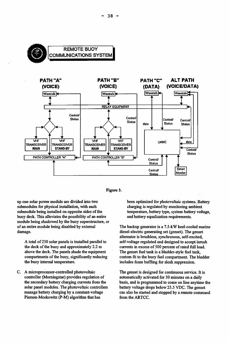
The communications system consists of four Park Air Electronics Model3070 VHF/AM transceivers for communications between the buoy and aircraft, four Westinghouse Wavetalk® L-Band satellite phones for communications between the buoy and the ARTCC, and the required voice relay (interface) equipment The communications path between the buoy and aircraft is VHF/AM radio; between the buoy and the satellite earth station, L-Band satellite; and between the earth station and the AR TCC, telephone land lines (Figure 1).

The communications channel on the primary satellite is a dedicated circuit. When a pilot or air traffic controller keys the microphone, dialogue can be initiated with no delay. The buoy-located radio relay function is virtually transparent to users, with a 500 ms propagation delay being the only difference between this and a direct air-to-ground radio contact

System status is transmitted as X.25 packet data via a dial-up L-Band satellite channel to the ARTCC and to NDBC. System status data are automatically

;;~~~J!daddad Z

kf ·::~~:··············································· .. ···········:.~ndaddad 1

~M~~~ i

VOICE PATH ATC <> AIRCRAFT

Main Satell~e: Dedicated Une Backup Satellite: Dial-up Une

j Sky Planet J _ _ _ ~

l ,kr-~~---------~ :.~MSAT, ~ : ~ Ottawa, CA : l ' .. -::·· :

i ,' (Skys~o) f ~ '' ,.·<.:::;}/ / \

I / I l .... / .. :~::::>< : \ Houston

FAA Communications ~uoy

Figure 1.

- 37 -

transmitted at predetermined intervals, or can be obtained at any time by an interrogation command from the ARTCC (Figure 2).

Tests have shown that the Wavetalk® antenna can maintain a lock on the satellite with buoy motion of up to 50° /s angular velocity and 28 o /s2 angular acceleration.

Redundancy is provided for all BCS equipment. There are two paths of communication with the primary satellite. Each path consists of one satellite phone, two transceivers, and other associated equipment. A third satellite phone can provide communications via a backup satellite. The data path and the local maintenance monitoring and control (LMMC) system also have redundancy (Figure 3).

3.3 BCS Power System

NDBC has designed and tested a buoy-mounted direct current (DC) power system capable of providing the large amounts of average and peak power required by the BCS. The primary power system consists of a photovoltaic array, photovoltaic charge controllers, secondary batteries, and a power system monitor and

control unit. A backup power capability is provided by a 7.5-kW auxiliary diesel engine generator set. The primary power system provides continuous average power in excess of 800 watts at 24 VDC and satisfies peak demands up to 5,000 watts without the support of the diesel generator. A block diagram of the entire power system is shown in Figure 4.

The primary power system is designed for graceful degradation in case of component failure or damage. The system is divided into 14 separate diode isolated 24-VDC sources. Each of the sources consists ofthe following:

A. Sixteen 12-V batteries (Sonnenschein Model 212/80A). Two 12-Vbatteries are connected in series to provide a 24-VDC unit, then eight of these 24-VDC units are connected in parallel.

B. Sixteen solar panels (Type M55J), each of which, at peak power, produces 3 .I amperes at 17.5 VDC. To produce the nominal 24 VDC required to charge the batteries, two panels, called a set, are connected in series, and eight sets are connected in parallel. Each set is diode isolated from the others. The eight sets that make

::~~LNOJHH z

!\y ·:::~::"""·············-·····················-·-····-·····:.~tsalldaridad1

DATA PATH RMMC <> LMMC

S Mexico City f

~~\ SkyP~Ianet ------------1---.,. X1P.~ SWitched-. TMI : ; "' ' .MSAT \ ~ ,

Data \ Ottawa, CA _,_ ; : , I \ (Skysite) ; ; f ' I ... _,_, :, I

~. , i' \ fl'!; ': I \. " x.25 ~ f I . , :

--.---_...r--~ .... \~~~r-"'1 ' j I

X.251' I , - - - - - .I Houston ,

" ,

NDBC sse. IllS

, i I , : , .

Figure 2.

Main: X.25 Packet Switched Data thN primary satellite Backup: RS-232 Modem line thru backup satellite

- 38 -

- REMOTE BUOY - COMMUNICATIONS SYSTEM

PATH .. B .. (VOICE)

ControV Status

PATH .. c•• (DATA)

data

ALT PATH (VOICE/DATA)

ControV Status

ControV Status

LMMC

ControV Status

ControV

ControV Status

Figure 3.

up one solar power module are divided into two submodules for physical installation, with each submodule being installed on opposite sides of the buoy deck. This alleviates the possibility of an entire module being shadowed by the buoy superstructure, or of an entire module being disabled by external damage.

A total of230 solar panels is installed parallel to the deck of the buoy and approximately 2.2 m above the deck. The panels shade the equipment compartments of the buoy, significantly reducing the buoy internal temperature.

C. A microprocessor-controlled photovoltaic controller (Morningstar) provides regulation of the secondary battery charging currents from the solar panel modules. The photovoltaic controllers manage battery charging by a constant-voltage Pierson-Moskowitz (P-M) algorithm that has

been optimized for photovoltaic systems. Battery charging is regulated by monitoring ambient temperature, battery type, system battery voltage, and battery equalization requirements.

The backup generator is a 7.5-kW keel-cooled marine diesel-electric generating set (genset). The genset alternator is brushless, synchronous, self -excited, self-voltage regulated and designed to accept inrush currents in excess of 500 percent of rated full load. The genset fuel tank is a bladder-style fuel tank, custom fit to the buoy fuel compartment The bladder includes foam baffling for slosh suppression.

The genset is designed for continuous service. It is automatically activated for 30 minutes on a daily basis, and is programmed to come on line anytime the battery voltage drops below 23.5 VDC. The genset can also be started and stopped by a remote command from the ARTCC.

- 39 -

MODULE ,

MODULE: 2.

MODULE: 14

NOTES:

1. lHE J MODULES SHOWN ME TYPIC'L OF A TOTAL OF 14 MODULES REQUIRED fOR 800 WATT CONTINUOUS LOAD.

[;:> lHESE SIGNALS (MODULE CHARGE CURRENTS, LOAD VOLTAGE) ME DIGITIZED BY "SMART• MONITOR AND SENT TO w.RS SERLA.L PoRT TO PROVIDE HOURLY POWER SYSTEM DATA.

Figure 4.

A BCS primary power system (without the diesel generator) has been tested at sea. The system was installed aboard a 12-m LNB, which was then deployed in the Gulf at Main Pass Block 163, which is approximately 40 miles south of Pascagoula, MS. The test was conducted using a load bank sized to draw 880 watts (1 0 percent above the required system power output) and ran for approximately 5 months, from June 24 through November 20, 1996. The system satisfied all test requirements with no exceptions and no failures.

An auxiliary power system which uses excess power generated by the BCS system (available during periods of low BCS use) charges five 24-V secondary batteries in parallel, each consisting of two 12-V batteries in series. This power is available to operate fan ventilation for the BCS compartment.

The NDBC meteorological package on the buoy is powered by a separate 12-VDC power system

consisting of five solar panels, one controller, and six secondary batteries.

The operational status of the BCS power system is monitored by an NDBC-designed smart monitor that measures system battery voltage, charging currents, and other related parameters and reports these values through a Multifunction Acquisition and Reporting System (MARS)-based meteorological data system via the GOES to NDBC. Power system data will also be transmitted with the remote maintenance monitoring and control (RMMC) system data through the BCS viaL-Band communications satellite to the ARTCC in Houston, TX.

The smart monitor will also control operation of the genset. It is programmed to run the genset on a predetermined daily operation schedule. The smart monitor will also start the genset anytime the system voltage drops below 23.5 VDC. The genset can be controlled remotely from the ARTCC in Houston via the communications satellite and through the NDBC

- 40 -

Operations desk via the GOES command receiver located on the buoy.

4.0 METEOROLOGICAL DATA SYSTEM

NDBC installs meteorological (Met) packages on all buoys deployed by the Center. The Met package on this buoy consists of dual, sonic (no moving parts) anemometers, air temperature sensor, barometric pressure sensor, a directional wave system, and a MARS data collection platform. The system reports on an hourly basis through the GOES data collection system.

5.0 BUOY COMMUNICATIONS SYSTEM STATUS

Factory acceptance testing of preproduction BCS No. 1 is now under way at NDBC. This system will be deployed at a site located in Main Pass Block 163 in

the Gul( The location is approximately 25 km ( 40 mi) due south of Biloxi, MS, with a water depth of approximately 46 m (150 ft).

Preproduction BCS No. 2 is now being built. This system will use Cubic Communications ATC-1 OOA transceivers. The tranceiver uses digital signal processing as opposed to analog, and costs only about 20 percent of what analog transceivers cost. The FAA will study the feasibility of using such transceivers in the future. Digital VHF transceivers have not been certified for use in the ATC system.

When the system is declared operational, two or three FAA buoys will be deployed in the Gulf of Mexico at a latitude of26°30', which is about 186 km (300 mi) south of the U.S. Gulf Coast, with one or two buoys located in the West Flight Information Region (FIR), and one in the East FIR (Figure 5). The water depth at these locations is approximately 3,124 m (10,250 ft) .

.,., BUOY 1 93• 42'W 26• 30'N BUOY 2 go• 42'W 26• 30'N BUOY 3 87• 22'W 26• 30'N KEY WEST RCAG SITE CORPUS CHRISTl RCAG SITE

Current NDBC Moored Buoys 42001 89° 65'W 25° 93'N 42002 93o 57'W 25° 89'N 42003 aso 91'W 25° 94'N

Figure 5.

- 41 -

The Cape Mudge Wave Experiments: Early Results by

M. Blaseckiet, S.G.P. Skey1, K. Berger-North1

, J. Ploegl and P.A. Bolducl

1.0 Background

On the West Coast of Canada between the northeastern end of Vancouver Island and the mainland, there is an important shipping route for all vessels (commercial and recreational) travelling up and down the coast. The southern end of this route is a narrow passage called Discovery Passage. To the north of Discovery Passage are Johnstone Strait and Queen Charlotte Strait, leading out into Queen Charlotte Sound, and to the south is the Strait of Georgia.

The tidal currents in Discovery Passage are extremely high, well known and predictable. They can reach speeds of 10 knots or so on the flood tide (southward flow) and slightly less on the ebb tide (northward flow). When a strong south wind coincides with a flood tide, an extreme wind-against-tide situation occurs, creating very hazardous wave conditions for all marine users. Slightly less extreme, but no less dangerous, conditions exist when northerly winds occur with an ebb tide.

In an attempt to monitor the wave conditions more specifically, and to provide round the clock accurate sea-states, in January 1997 a directional 0.9m diameter Datawell waverider buoy was installed near the southern e~ of the Discovery Passage in an area known as Wilby Shoals. The buoy was located 1/2 mile to the east of the entrance to Discovery Passage in a water depth of 30 m, with good open exposure to the south and south west, but limited exposure to the east and north. Figure 1 shows the location of the wave experiments. The reason that the waves were measured at Wilby Shoals and not in Discovery Passage itself are given below.

The wave data were transmitted to a meteorological station at Tyee Spit (on Vancouver Island about 5 miles to the west) where they were integrated with meteorological data gathered at Tyee Spit. The integrated data were then formatted for Environment Canada who accessed the data on an hourly basis via telephone modem. These data were then used in the Environment Canada and Canadian Coast Guard bulletins. All of these data were downloaded and archived by the Marine Environmental Data Service of the Department of Fisheries and Oceans.

Although the wave measurement program at the edge of Wilby Shoals was successful, and the buoy remained on station till the end of the project funding in May 1998, the wave conditions were very different from those experienced at the entrance to Discovery Passage. This was because the waves measured at the Wilby Shoals site were not affected by the strong tidal currents found in Discovery Passage.

1 Axys Environmental Consulting Ltd., Sidney, B.C., Canada.

2 Formerly with DFO/Canadian Coast Guard, Vancouver, B.C., Canada.

3 Marine Environmental Data Service, Ottawa, Ontario, Canada.

- 42 -

.~ · ~p

- 43 -

To research this and provide a solution two supplementary studies were carried out. The first was to validate the data being gathered at Wilby Shoals with the data gathered at a buoy at Sentry Shoal 8 miles to the south. A second study was to modify the directional wave spectra gathered at Wilby Shoal by taking into account the tidal currents in the Discovery Passage.

2.0 Measurement of Waves in Discovery Passage

There are only three ways to measure waves. These are from the surface, from the subsurface and remotely. Each of these options is examined below.

2.1 Measurement from the surface

Traditional measurements of directional wave spectra from the surface use a small buoy (approximately 1 m diameter) in which a series of accelerometers are mounted. The motion of the buoy is assumed to represent the motion of the waves, and these motions are sensed by the accelerometers. Analysis of the accelerometer data lead to formation of directional wave spectra and information about wave height, period and direction. However these buoys are limited to working in maximum currents of no more than 6 knots (3 mls) because in larger currents the strain on the mooring line is so great that it affects the ability of the buoy to move freely with the waves. In very high currents the buoy may be pulled under the surface. This is a severe limitation in Discovery Passage where the currents are much higher than the maximum practical values for a surface following buoy.

A further difficulty with measurement of waves from the surface in Discovery Passage is that with the high volume of marine traffic through the narrow passage, the buoy is very likely to get hit and destroyed. A significant problem for a proposed permanent wave monitoring program.

2.2 Measurement from Sub-Surface

In relatively shallow waters (<50 m) it is possible to measure waves by sensing the pressure differences on the bottom. Unfortunately Discovery Passage is too deep for this method being approximately 90 m. In some circumstances it is possible to mount a pressure sensor at mid depth on a mooring. However this method is not practical in areas with extremely high currents, because of the difficulty in maintaining the mooring. Also in Discovery Passage the presence of large numbers of tugs and barges with hanging towlines are likely to destroy any shallow sub-surface mooring.

2.3 Remotely Sensed measurements

Although shore based radar (CODAR) are mainly used for measuring currents through Doppler shift technology, they can measure waves. However since the primary returns indicate current speed and direction, in a high current regime the signal for the wave heights would be swamped.

A shore-based wave radar is also not suitable since the actual wave heights rely on a downward looking altimeter.

- 44 -

Given the above it is clear that it is not practically possible to physically measure the waves in Discovery Passage.

3.0 Wave Calibration and Validation

3.1 Field Verification

3.1.1 Verification of waves measured on Wilby Shoals

Axys installed the Datawell directional wave rider buoy on Wilby shoals near Cape Mudge at the entrance to discovery Channel in late January 1997 in 20 m of water ( 49°59'N 125°09W). The wave data and sea temperature data are transmitted via VHF to the Canadian Helicopters hangar at Campbell River. At the hangar, wind speed and air temperature are also measured. The wind and temperature data are combined with the wave and sea temperature data and made available to Environment Canada and Coast Guard.

The Environment Canada Sentry Shoal ODAS weather buoy is located in Georgia Strait eight miles to the SE of Discovery Channel in 18 m of water. The following report gives a brief comparative analysis for data sampled in February and March 1998 for Discovery Channel (DISCO) and Sentry Shoal (46131).

3.1.1.1 Data

The data are gathered as follows:

3.1.1.2

• Winds: Wind speeds are calculated from a ten-minute mean, both at the Sentry Shoal buoy and at Discovery ChanneL

• Waves: The sensor in the waverider buoy is comprised of 3 vertically stabilised accelerometers. The sensor in the 3 m buoy is a strap-down accelerometer. It does not measure wave direction. The significant wave height is calculated from a twenty minute record every hour. The significant wave can be regarded as the mean height of the highest third of the waves. This correlates with the "visual" appearance of the sea state. The value of the significant wave is a standard calculation from the spectral variance.

• Temperature: The air temperatures are calculated over a ten-minute mean.

Data Plots

Figure 2.1 shows time series data for wind speed (m/s) and direction (0), and significant wave height

(m) for both Discovery Channel (DISCO) and Sentry Shoals (46131) for the period ofanalysis in February. Figure 2.2 shows similar parameters for March. The tidal current shown is for Discovery Passage.

- 45 -

Mid February 1998 Wind Speed

20 .... ····-·-·········-···· ............ _, ....... -..................................... _, __ , .................. --.. ---·--·--·-·---·---·--· .... -.......... -...... ___ ,,,_ .. _ .. ___ , ................ ___________________________ , ___ ,,.,,.,, ___ _

5~-------;~7ft~~--------~--~~~----~~~~------~~~~~

O~mm~mmmm~mmmmmmmmmmmm~mmmmmmmmmm~mmmm~~~mm~mmmmmm~

400 350 300

... ---·- -·-·-.. ---·----......

Mid February 1998 Wind Direction

--- .

fl) 250 ~ 200 f 150

• l\ A A

JiNVI

100 50 0

IJ\ I"\.

~"-1,1~·-..,~ ----o-

.... CX)

}. ',.,, .. "'-. ---~ ,,.,_ ....:. .rv'1· --·- ~.-

·~

Mid February 1998 Hs

. ... .,. ,, ,. ·r:""' ~v'¥

~ \)

3.5 ------------------------------------------------------~ 3+---------------------~~------------------------------------~

2.5+---------------------~~------------------------------------~

2+-------4T----------~~~------------------------------------~ E1.5+-----~~~------~~~~~r---------------------------------~

1 +-~~~~~--~~~~----~~~--~~~~~~------------~~~ 0.5~~--~--~~~----------------~~------~~~------~~~~~

o~~~~~~~~~~~~~~~~~~~~~~~~~~

9 17 25 33 41 49 57 65 73 81 89 97 105 113 121 129 137 145 153 161

Mid February 1998 Tidal Current (Flood+)

10 8 6 4

.!!! 2 E 0

-2 -4

-6

-8 Hourly Data

Figure 2.1

••••• ·46131 --DISCO

, «5' c: ca 1\)

N

:c 0 c ~ c &

mls Q,(nj..~ON~cnc:o

3: a: 3: m ~ ::r

'3~ OCD 0· co t::t -a.

!!. 0 c a :I -

31

43

49

55

61

67

73

79

85

91

97

103

109

115

121

127

133

139

145

151

157

163

m oooo ~~

oN~mi»~N~

z

.. ,

3: a: 3: m

~ -CD CD co

if

1

7

13

19

25

31

37

43

49

55

61

67

73

79

85

91

97

103

109

115

121

127

133

139

145

151

157

163

·degrees ~-1'\)1'\)(a)(a)~

U\OU\OU\OU\0 000000000

28; rn~ ow 0 ~

mJs - ~ 0 N ~ en CO 0 N

1 ~ I RJ I I 7

13

19

25

31

37

43

49

55

61

!! 67

3: a. 73 a: 3: m 79 3: ~ m ::r ~ - 85 ::r .a:=. CD - 0'\ U) CD C!O 91 CD

~ co

:I 97 ~ a. :I c 103 a. a (/) , ~ 109 .. : 0 a. :I 115

121

127

133

139

145

151

157

163

- 47 -

3.1.1.3 Analysis

a) Wind

The wind data do not show any surprises. The wind speed is generally higher at Sentry Shoals by a few metres/sec. The patterns for the wind speed are similar for both locationS.

b) Waves

The wave heights from both sites are similar and display similar patterns. In particular it is important to compare the wave heights with the wind speed as well as the wind direction. When the wind direction is from the south or southeast, the wave heights at Discovery Channel are proportionally larger than for a similar wind speed from other directions. This is because the waverider is partially sheltered from winds from the west, north and northeast.

c) Sea Surface Temperature (SST);

The SST values (not shown here) from the buoy at Discovery Channel show a relationship with the tidal cycles. It appears that during the northerly flowing ebb tides the SST rises slightly. This might be explained by the movement of the warmer surface waters of the Georgia Strait.

d) Air Temperature

The air temperature values (not shown here) match each other quite well. The greater variability at Discovery Channel can be explained by the fact that these values are not over water values. They are measured on land at an elevation of 10 metres. The buoy-measured winds are at an elevation of approximately 5 m.

3.1.1.4 Surmruuy

The data show that there is little substantive difference between the two sites, especially when the winds are from the southern sectors. The SST values may differ more markedly during the summer season, and are typically ~ore variable at Discovery Channel on a diurnal basis.

3.2 Modification of Waves According to the Currents

It is known that a wave field is modified in the presence of currents. Recent research (Nwogu, 0. 1993) has indicated that it is possible to predict how the directional wave spectra will change if the current speed and direction is known. At Discovery Passage the magnitude and direction of the currents are known and predictable, since tidal forces drive them. Also the directional wave spectra within 112 mile of Discovery Passage at Wilby Shoals are known. Thus by modifying the known wave spectra with known currents it may be possible to estimate the existing wave conditions in the passage.

- 48 -

This following section describes the modification of the Wilby Shoals directional wave spectra with Discovery Passage currents. It also describes an attempt to verify these modified waves with actual measured waves from a dedicated vessel over a flood tide event.

3.2.1 Discovery Passage Tidal Currents

The current speed and direction values for Discovery Passage were obtained from Fisheries and Oceans at the Institute of Ocean Sciences, Sidney, BC. The scientists there have modelled the entire Georgia Strait and are in the process of verifying the modeL However at the time that the present work was taking place the verification process had not been completed. So in the meantime the known currents modelled from Seymour Narrows (a mile or so to the north of Discovery Passage) were modified for Discovery Passage. This modification, which took into account both height and temporal modifications was only approximate. However the opinion was that for this pilot project stage it would give a reasonable account of $e currents at Discovery Passage.

The modifications for Discovery were a reduction from the Seymour Narrows predictions. of a factor of 111.75 for flood speeds and of 1/2.20 for ebb speeds. The times were not adjusted since observed currents at both sites suggest time adjustment is small if not zero.

The outcome of this work was a database of hourly data for a whole year of current speed and direction at the entrance to Discovery Passage.

3.2.2 Modification Algorithm

The software required to modify the directional spectra was developed at the CHC of the NRC. Dr. Okey Nwogu's research both theoretical and in model tests in the wave tank at the NRC in Ottawa, indicated how the effects of current speed and direction modify wave spectra. The algorithm was made available to the project. These modifications include an algorithm that limits the steepness of the waves.

3.2.3 Integration of Current Speed and Direction Database and Wave Modification Algorithm.

The wave analysis software of NRC and the current speed and direction database was integrated with the existing system installed in place at the Base Station at Tyee Spit. The Base Station software took the hourly measured spectra from Wilby Shoals, and the predicted current speed and direction for the same hour from the database and then modified the spectra in accordance with the NRC algorithm. The resulting spectra were then analysed to provide a value of the "simulated" significant wave height. This wave height was then inserted into the hourly message that was formatted for Environment Canada and Canadian Coast Guard.

3.2.4 Real Time System

The system was installed and operated in real time for three months from January to the end of March

1998.

- 49 -

3.2.5 Verification

Once the system was operating, we planned to carry out a verification program. As discussed above since it was not possible to measure waves in Discovery Passage with any automatic systems, we had to use a dedicated vessel following a free-floating waverider.

3.3 Measurement of waves in Discovery Channel

The wave model validation trials were completed on Wednesday January 14/1998. The weather forecast for Tuesday pm was for gale to storm force SE winds in the northern Strait of Georgia continuing into Wednesday. The equipment used for the trial was a Datawell 0.7 m Waverider buoy with DIW AR radio receiver, autotrack GPS receiver and PC computer data logger/processor. The Waverider was prepared for a fiee floating deployment with 2 ballast chains secured beneath the buoy and a 15m pickup line terminated with a Scotsman float. A portable autotrack GPS receiver was attached to the head of the buoy and programmed to log a position once a minute. All data was transmitted form the buoy to a logging station on the research vessel

The timing of the currents at Discovery Passage was such that the turn of the tide was at 13:05 with the maximum flood current predicted for 15:41 hours. The predicted current speeds for the times of the trials, namely 13:30, 14:30 and 15:30 were approximately 0, 3.5 and 4.3 m/s (See Figure 3).

There were a total of three drift deployments run during the afternoon. The maximum currents as calculated from the GPS data were 3.5 knots at approximately 15:30. The weather for the first two tracks was clear with 15 knot SE winds. The weather for the third track deteriorated with winds gusting to 25 knots, rain squalls reducing visibility and coupled with maximum flood currents. Plots of the three buoy tracks are shown in Figure 4.

~ Discussion

The following observations from the field evaluation were made:

• The current regime in the area was quite complex with a high degree of variability both spatially and temporally,

• High occurrence and rapid generation of potentially dangerous waves;

• Although the conditions the trials were not run under most serious wind/wave conditions likely to occur in the area, it would have been dangerous to consider the operations in much more than was encountered. The waves in the rip area although not large tend to be very steep and breaking.

1/)

C'tl 'i: ..,_ r::: 0 .. C'tl

"'0

C'tl > C) r::: 'i:

:::::1

0 Q) C) C'tl 1/) 1/) C'tl a. ~ Q)

> 0 0 1/)

0 '-.2 1/) -r::: ~ '­:::I ()

C'tl "'0 ~

l{) 0 l{)

- 50 -

(/)

c - (]) ~ t: ...... ::J ...... ()

8 ~ (/) ~ !': 0 0 L) t: (/) ro 0 z ...... -c ::J (]) 0 t5 E :0 >. (]) (]) ......

II

0

SJW

0 l{) .,.... .,....

I I

- 51 -

Observations from Drift Deployments

Trial Run Time Waverider WUby Shoals Sentry Shoals Discovery (0.7 m) Waverider (3 m Discus Buoy) Passage

(0.9 m) measured (simulated)

13:30/21:30 UTC 0.47m/5.9s 1.2m/3.9s 1.5m/5s

14:30/22:30 UTC 1.02m/5.1s 1.3m/4.1s 1.0m/5s

15:30/23:30 UTC 1.36m/4.9s 1.2m/4.9s l.Om/4s

3.3.2 Wave Modification Algorithm

The algorithm used (Nwogu, 1993) to modify the spectra was successful for situations where the currents were in the same direction as the winds, but only partially successful in true wind-versus-current situations. When the current values exceeded -1 rn/s, the higher frequency end of the spectra reduced to zero. As the current speed increased to -2 or -3 rn/s this end of the spectra shrank toward the lower frequency end such that at -3 rn/s there was no spectra left at all.

The reason for this is that with adverse currents, there is maximum current speed at which the waves cannot propagate into the currents and will be reflected. Based on kinematic considerations alone, the maximum current speed is equal to the local group velocity. In deep water,

U_block = -0.25 Phase Velocity (without currents).

As you approach that speed, however, there will be significant non-linear interactions and wave breaking. To properly study such steep waves in adverse currents, a fully non-linear wave current interaction model with wave breaking is required.

4.0 Summary and Conclusions

This program was unique and had a number of unique challenges. The observations from the field during moderate wind versus tide conditions underscored the difficulties is monitoring wave. conditions in these situations, either from a research vessel or remotely via instrumentation.

The methodology used to simulate the actual spectra had a number of source errors. These were:

• No knowledge of the actual current speed and direction in the area. The data used was taken from an uncalibrated model which seemed to provide reasonable numbers;

• The current speeds and directions in the area were highly variable both temporally and spatially;

• The algorithm used (Nwogu, 1993) to modify the spectra was not a fully non-linear wave current interaction model with wave breaking.

- 52 -

As such, wave accuracy could not be expected to be within the 3% estimated by the waverider. From pragmatic considerations wave height values (Hs) within 0.5 m would be considered acceptable.

Unfortunately the project funding was terminated before the analysis could be completed and modification model assessed further. However there was definitely enough infonnation and positive results from this program to give a cautious thumbs-up for this pragmatic and possible method of trying to provide real-time values of wave heights within acceptable error limits in situations where strong currents and deep water prevent the waves from being measured directly.

5.0 References

Nwogu, 0. 1993. Effect of steady currents on Directional Wave Spectra, OMAE, Volume l, Offshore Technology, ASME.

Note: The above desaibed wak was sponsored by the DRJ/Canadian Coost Guard and Axys Environmental Systems, with assistance from the Canadian Hydraulics Centre (CHC) of the National Research Council.

. . . . . . . .... .

'\23:43:42

Figure 4: Buoy Tracks

- 53 -

SEPARATION OF SEA AND SWELL FROM NDBC BUOY WAVE DATA

David W an'i and David Gilhousen2

Computer Sciences Corporation1 and National Data Buoy Center Stennis Space Center, Mississippi, USA 39529-6000

1.0 INTRODUCTION

The National Data Buoy Center (NDBC) operates more than 50 buoy stations reporting wave spectral data hourly. From these spectra, real­time reports of significant wave height and dominant wave period were posted on several Internet home pages for the last 2 years. One frequent request from the maritime public using these postings was to add swell height and period measurements. Indeed, wind seas and swells have different characteristics that are important for seakeeping safety, small boat operation, ship passages over harbor entrance, and surfing forecasting (Earle, 1984). The statistical description of individual wind sea and swell wave system provides information needed to investigate the influence of swell on wind sea growth and dissipation in open ocean (Hanson, 1996). The presence of swell could also affect the relationship between wind stress and sea state (Dobson, et al. 1994).

A wave identifying and tracking scheme was formulated for directional wave spectra (Gerling, 1992; Kline and Hanson, 1995; Hanson, 1996). This approach requires information of both directional wave and wind data that may not always be available. Earle (1984) proposed that the frequency separating wind seas and swells are related to the peak frequency of the Pierson-Moskowitz (P-M) spectral model, which can be determined for a given local wind speed. This approach is conceptually similar in that wind sea is part of the wave spectrum for which the wave phase velocity is less than the wind velocity component in the direction of wave propagation (TheW AMDI Group, 1981; Dobson, et al. 1994). Vartdal and Barstow (1987) developed an algorithm, based on the shape of mean JONSWAP spectral model, to separate

wind seas and swells for a given wave spectrum that does not require wind data.

In this study, in addition to algorithms by Earle (1984) and Vartdal and Barstow (1987), a new algorithm for separating wind sea and swell based on wave steepness was introduced. Three algorithms were examined using directional wave and wind data collected from a buoy station off the Alabama coast in the Gulf of Mexico.

2.0 ALGORITHMS FOR SEPARATION OF WIND SEA AND SWELL

The separation of wind sea and swell is carried out by estimating separation frequency,/51 for the wave spectra. Wave energy at frequencies higher than fs is considered generated by local winds; wave energy at frequencies lower than fs is considered generated by swell. Three algorithms for estimatingf5 are introduced.

2.1 P-M Algorithm

According to the P-M spectral model, the peak frequency of a fully developed sea is related to the local wind speed by

f. = 1.25 p u (1)

where /p in Hz is the frequency of maximum spectral density and U in m/ s is wind speed at the 10-m height. Earle (1984) recommended the separation frequency Is as

fs = CJ, (2)

where C is an empirically determined constant. A value of0.8 is used by Earle (1984). A similar approach with additional consideration of the wind and wave direction difference was developed by Vartdal and Barstow (1987).

Submitted by the co-author for the presentation "Estimating Swell Infonnation for NDBC's Web Site." Paper originally prepared for 5th International Workshop on Wave Hindcasting and Forecasting.

- 54 -

Equation (2) with a value of 0.8 for C can be expressed as the relation of wave phase velocity, V 51 at Is and wind speed, which is

Vs = 1.56U (3)

This suggests that Earle's algorithm is similar to the concept that wind seas are reflected in a specific frequency range of the wave spectrum.

2.2 Spectral Shape Algorithm (SPSH)

The spectral shape algorithm, denoted as SPSH, was developed by Vartdal and Barstow (1987). This algorithm is based on the shape of the mean JONSW AP spectrum. The first step is to determine the lowest frequency .fi of wind-generated equilibrium range that has

sif)*f5 > 2.5*10-4(m 2Hz 4) (4)

where slfJ is the measured wave spectral density in m2/Hz andfis frequency in Hz. The value 2.5*104 is half the asymptotic value of the P-M spectrum multiplied byf5

• The second step is to determine the wind sea peak,fwil that is the frequency of maximum SlfJ in the range

0.75ft < f < 1.25ft (5)

and takes

f. = c~ s :lwi (6)

as the separation frequency between swells and wind seas. C is an empirically determined constant. A value of 0.75 is used by Vartdal and Barstow (1987).

2.3 Wave Steepness Algorithm (STPN)

The wave steepness algorithm, denoted as STPN, is based on the assumption that wind seas have higher steepness and swells have a lower wave steepness. A representative parameter describing the steepness of random waves is defined as

Hs 21Cils steepness = L = --

2 (7)

gTz

where H5 is the significant wave height, L is the

wave length associated with Tv and T z is the average wave period computed from the nth moment of wave spectrum by

H,=4Fo, T,=~~ m = fi"Jnslf)df

n J1i

(8)

where fu and .fi are usually the upper and lower frequency limits of measured wave spectra, respectively. In this study, 0.03 and 0.4 Hz were used for the lower and upper limits, respectively. A frequency-dependent parameter representing wave steepness over frequencies ranging from a specified f to the upper limit fu is defined as

~(f) = 21tH/f) gT/f)2

where H5(/) and TzlfJ are computed from

(9)

1-71\ ~ "'olf) ~(f)=~"~VJ' ~(/)= -----"'-lif) (10)

m (f) = fi"Jns(f)df n Jf

The separation frequency fs is estimated by

fs = Cfx (11)

where fx is the frequency of maximum ((fJ, and C is an empirically determined constant. A value of 0.95 is used in this study. This method does not require wind data and any assumption concerning wave spectrum.

3.0 FIELD DATA TESTINGOFTHE SEPARATION METHODS

The validity and reliability of the algorithms were examined using hourly measured wind and directional wave data measured from an NDBC buoy station during a meteorological frontal passage accompanied by rapid wind speed and direction shifts. The buoy was moored off the Alabama coast at a water depth of approximately 30m. The buoy was equipped with an NDBC directional wave measurement system to estimate wave directions using the buoy's heave,

- 55 -

pitch, and roll motions. Winds were measured by an R.M. Young propeller-type anemometer mounted at the top of the buoy mast at approximately 5 m above the waterline. The 5-m measured wind speed was converted to wind speed at a 10-m height using a multiplication factor of 1.2.

As the wind direction remained approximately 140 degrees during the first 26 hours from December 13-15,1995, the wind speed gradually increased from 5 to 15 m/ s (see Figure la). The significant wave height increased from 0.5 to 4 m as the dominant wave period increased from approximately 4 to 8 s (see Figure lb). The wave condition during this period was dominated by wind seas caused by the long-fetch southeasterly winds over the Gulf of Mexico. In the early hours of December 14, the wind speed quickly dropped to less than 4 m/ s as wind direction shifted to approximately 290 degrees. Wind speed then increased to approximately 10 m/s, and both the wind speed and direction remained relatively steady for the

-speed o direction

rest of the period. The wave conditions during this period consisted of southerly swell and a newly developed wind sea generated by the fetch-limited northwesterly winds.

Figure 2a shows a selected wave spectrum with significant wave height of 4.135 m and wind speed of 15.3 m/s before the frontal passage, which are the highest wave height and wind speed of the entire period. Figure 2b shows frequency-dependent mean wave direction that aligned well with the local wind direction as indicated by the horizontal dashed line. The separation frequencies derived from the P-M, SPSH, and STPN algorithms are indicated by the vertical dashed, dash-dotted, and solid lines, respectively. The vertical dotted line shows the frequency above which the deep-water wave phase velocity is less than the wind velocity component in the mean wave direction. As shown, separation frequencies from the above algorithms are lower than peak frequency at 0.13 Hz, indicating wave energy is mainly generated by the local wind.

150

100

o~--~----~----~--~----~----~--~----~--------~50 13 13.2 13.4 13.6 13.8 14 14.2 14.4 14.6 14.8 15

December, 1993

_5~~~========~---------------------------------------------.10 .§. (b)

0

-height o period

0 00 0

oooo

0 000 oooooo

00

0000 00 0 0 0 0000 00 0

000 -() (J) (/J -

- 56 -

Station 42016 93/12/14, 2 UTC, HS= 4.135 m, U= 15.3 m/s

(a) --P-M

·-·- SPSH -STPN

oL-----WL--dGL---~----L~~~~~--~----~---~---~ 0 0.05 0~ 1 0.15 0.2 0.25 .o.3 0.35 0.4 0.45 0.5

frequency (Hz)

c; CD -c

300

1-

. I

(b)

I

. '

-- winddir . 0 wavedir

. I . 0 0 0 i: lo o o oo o o o .P

I i#: -~---· eot:>-ooo~oooe-aOn-crooo--- -e-o-a.--- -or>c:o . :

~200 0 = !

0 I I . I :

I : =a 100

I I :

- 'I : .. I t t t ' "" 0

0 0.05 0.1 0.15 0.2 0.25 0.3 0.35 0.4 0.45 0.5 frequency (Hz)

Figure 2. A selected (a) wave spectrum and (b) mean wave and wind directions before the frontal passage. The separation frequencies derived from the three algorithms are indicated by the vertical dashed, dash-dotted, and solid lines. The vertical dotted line indicates the frequency above which the wave phase velocity is less than the wind velocity component in the mean wave direction.

Figure 3 shows the selected wave spectrum and mean wave direction of a bimodal sea after the frontal passage. As indicated by the mean wave direction and local wind direction, wave energy at frequencies lower than 0.17 Hz has a major peak at 0.13 Hz, which was caused by swells coming from 160 degrees. Wave energy at frequencies higher than 0.17 Hz has a peak at 0.21 Hz, which was from wind seas generated by the local winds. The separation frequency derived from the STPN algorithm is 0.16 Hz, which properly separates the wind seas and swells. However, the separation frequencies from the P-M and SPSH algorithms do not separate the two energy sources properly. Using separation frequencies from these two algorithms for this bimodal wave spectrum overestimates wind sea energy and underestimates swell energy. Examinations of wave spectra from the rest of the period show similar results as the two examples discussed.

The significant wave height and average wave period for wind seas and swells can be computed

from Equation (8) by replacing.fi with Is for wind seas and replacingfu with Is for swells, respectively. Figures 4 and 5 show the time series of wind sea significant wave height, H5w, and swell significant wave height, H55, obtained using the separation frequencies by the three algorithms. For comparison, reference significant wave heights for wind sea and swells are also shown. The reference wave heights are obtained by considering.fs as the frequency above which the wave phase velocity is less than the local wind velocity component in the mean wave direction. This separation frequency is indicated by the dotted vertical line in Figures 2 and 3.

As shown in Figure 4, when wave field was dominated by the growing wind seas before the frontal passage, the Hsw derived from the three algorithms all agree well with the reference Hsrv. During coexistence of wind seas and swells after the frontal passage, the H5w by the P-M and SPSH algorithms is significantly higher than the reference Hsw· The Hsw by the STPN

- 57 -

Station 42016 93/12/14, 13 UTC, Hs= 2.398 m, U= 11 m/s 10r----.----.----.---,----,---~----.---r=======~~

'Na

~ 6 .§.

~4 c -8 2

300

! ~200• :8

~ 100fo

(a)

0.05 0.1

--P-M

·-·- SPSH -STPN

0.15 0.2 0.25 0.3 0.35 0.4 0.45 0.5 frequency (Hz)

(b) ol I !' , . I I --~!- - --- - :_ - -a;- - :'Ot)O'OOO~ JJ_ C) -D- Q _p_ & _OJ 'b 1"" ! ¢ 0 oo o0oo o

oo ol Oi o;

: ! 0 : p ooo0c

I I I I I I

-- winddlr o wave dlr

oL-~~--~~~~~------~·WL~-L------~·---~------~·~==~====~==~ 0 0.05 0.1 0.15 0.2 0.25 0.3 0.35 0.4 0.45 0.5

frequency (Hz)

Figure 3. A selected (a) wave spectrum and (b) mean wave and wind directions after the frontal passage. The separation frequencies derived from the three algorithms are indicated by the vertical dashed, dash-dotted, and solid lines. The vertical dotted line indicates the frequency above which the wave phase velocity is less than the wind velocity component in the mean wave direction.

significant wave height of wind seas 5~---~------~---~------~------~---~------~---~-----~---~

--P-M

·-·- SPSH -STPN

o reference

I \.. ,, I \·I' I \- \

I \,"-""·-1 ~ ~ 1 'v""-'v,.\' I .. I " I I I

I I

I I OoO I I ., 00

0

oo o~----L------~---~------~------~----L------~---~-----~---~ 13 13.2 13.4 13.6 13.8 14 14.2 14.4 14.6 14.8 15

December, 1993 Figure 4. Time series of significant wave height of wind seas using the separation frequencies by the three algorithms. The reference significant wave heights for wind seas are obtained by using the separation frequency above which the wave phase velocity is less than the wind velocity component in the mean wave direction.

- 58 -

algorithm agrees well with the reference Hsw, except for a few hours when both wind speed and direction changed rapidly during the frontal passage.

As shown in Figure 5, when wave fields were dominated by the growing wind seas, the swell significant wave height, H55, by the three algorithms and the reference H55 are generally less than 1 m, and the differences among them are insignificant. When the wave fields consisted of wind seas from fetch-limited wind seas and swells, H55 by the STPN algorithm agrees well with the reference HSSI while H55 by the P-M and SPSH algorithms are significantly lower than the H55 by the STPN and the reference H55•

Figures 6 and 7 show the time series of significant wave height and average wave period of wind seas and swells·by the STPN algorithm, respectively. When wave conditions were dominated by wind seas before the frontal passage, the significant wave height and average wave period are almost the same as those of wind seas. During coexistence of wind seas and

swells after the passage on December 14, the separation algorithm provided a detailed description of the evolution of wave conditions. It shows the gradually decreasing significant wave height H5, in fact, consisted of a growing Hsw and a decaying H55 with an average wave period of approximately 4 s for wind seas and 7.5 s for swells.

4.0 SUMMARY

Three empirically developed algorithms for separation of wind seas and swells were examined based on directional wave and wind data from an NDBC buoy station during a meteorological frontal passage. All three algorithms provide similar estimation of separation frequency when wave conditions were dominated by wind seas from a uniform and long-fetch wind field before the passage. However, when wave conditions were contributed by both wind seas and swells after the passage, only the algorithm based on wave steepness {STPN) provided proper and

significant wave height of swells

0.

--P-M

·-·- SPSH -STPN o reference

0

9~ I 10 I I I I 0 I 1 0 I 1 I I

13.2 13.4 13.6 13.8 14 14.2 14.4 14.6 14.8 15 December, 1993

Figure 5. Time series of significant wave height of swells using the separation frequencies by the three algorithms. The reference significant wave height for swells are obtained by using the separation frequency below which the wave phase velocity is greater than the wind velocity component in the mean wave direction.

- 59 -

significant wave height by STPN method

4.5 -- seas & swells

0.

4 o seas

+ swells

+ + + +

+++ + + + +++++++++++++ +

+ +

+

o~-~~-~--_.--~--~--._--~-~~-~--~ 13 13.2 13.4 13.6 13.8 14 14.2 14.4 14.6 14.8 15

December, 1993 Figure 6. Time series of significant wave height of wind seas and swells by the wave steepness algorithm (STPN).

- seas & swells

o seas

+ swells

+

+

average wave period by STPN method

+

o~-~---L----~--._-~ ____ _. ____ ~ ___ ._ ____ ~--~ 13 13.2 13.4 13.6 13.8 14 14.2 14.4 14.6 14.8 15

December, 1993 Figure 7. Time series of average wave period of wind seas and swells by the wave steepnessalgorithm(STPN).

- 60 -

consistent separations for wind seas and swells. The other two algorithms overestimated wind seas and underestimated swells.

The STPN algorithm, without the requirements of wave direction, wind data, and wave spectrum shape assumptions, shows the spectral­related steepness parameter can be used to separate wind seas and swells effectively. This simple algorithm can be easily implemented to report wave height and period of wind seas and swells in real time for operational purposes.

5.0 REFERENCES

Dobson F.W., S.D. Smith, and R.J. Anderson, 1994: Measuring the relationship between wind stress and sea state in the open ocean in the presence of swell. Atmosphere-Ocean 32 (1), pp. 237-236.

Earle, M.D., 1984: Development of algorithms for separation of sea and swell. Technical Report MEC-87-1, National Data Buoy Center, pp. 53.

Gerling, T.W., 1992: Partitioning sequences and arrays of directional ocean waves spectra into component wave systems. Journal of Atmospheric and Oceanic Technology, Vol. 9, pp. 444-458.

Hanson, J.L., 1996: Wave spectral partitioning applied to the analysis of complex wave conditions in the north Pacific Ocean, in Proceedings, 8th Conference on Air-Sea Interaction and Symposium on Goals, America Meteorological Society.

Kline, S.A., and J.L. Hanson, 1995: Wave identification and tracking system. Technical Report STD-R-2436, The Johns Hopkins University, Applied Physics Laboratory; Laurel, MD.

Vartdal, L., and S.F. Barstow, 1987: A separation algorithm for wind sea and swell for applications to directional Metocean data buoy. Technical Report, Oceanographic Center, SINTEF Group, Trondheim, Norway, pp. 104.

TheW AMDI Group, 1988: The WAM model-A third-generation ocean wave prediction model. Journal of Physical Oceanography, Vol. 18, pp. 1775~ 1810.

- 61 -

Recovery of Near Surface Velocity from Undrogued Drifters

Stephen E. Pazan

Ocean Prospects, Encinitas, California

Peter P. Niiler

Scripps Institution of Oceanography, La Jolla, California

ABSTRACT

We have quality conttolled a global dataset of wind and buoy ~ made comparisons of 15 m drogued mJ

undrogued buoy observations, and developed both 1-D and 2-D linear regression models of the difference

between drogued and Wldrogued drifter velocity as a function of wind and Coriolis parameter. Meridional

and zonal surface wind velocity components from the global synoptic fNMOC model and the global

synoptic ECMWF model were interpOlated to each naval ANIWSQ-6 and WOCFJfOGA buoy position alXl

date/time in the datasets. Seven 1-D linear regression models were evaluated for both the Navy vs. WOCE

drogue-on dataset and the WOCE drogue-off vs. WOCE drogue-on dataset. Principal results from this

analysis were: the constant tenn in the regression analysis was zero; the Navy buoys behaved like WOCE

drogue-df buoys; either FNMOC or ECMWF winds were sufficient The 2-D regression analysis on

selected synoptic data was:

U unJrogwd - U drogued = B · W'

where U wtdnJped- U droruetJ was ensemble mean buoy velocity difference and W was wind velocity; the real am

imaginary pans of these quantities were the zonal and meridional components, respectively. B was the

complex valued regression coefficient We found that the absolute value of B was a function of the

reciprocal of the square root of the Coriolis parameter, f, giving:

8/28/98:9:33 AM

Submitted for publication to the Journal of Atmospheric and Oceanic Technology.

- 62 -

where the best fit gives Bo=-0.003, and 8 1=0.00016 (sec112). A dataset assembled from undrogued (Navy)

and drogued buoy pairs was. analyzed and results confinn the amplitude of the mean coefficient. The

analysis also found that the angle, J\, of the velocity difference with respect to the wi~ was a function of

the. surface wind and the CorioliS }maDlCtel':.·

ll= Phas(Bl= (A,.+ A, ·-twr· /-112),

where A. ranged from 20° to 35° to the. left (right) of the wind nortli (south) of the equator from 111' to srr

in latitude;· it is best fit by Ao =IS' am A.,= O. 75 (degrees ~/m).

A pammetric model of the Ekman spiral plus a leeway was used to evaluate the observed velocity·

differences. The parameters derived from non-linear regression analysis were consistent with Ralph & Niller

(1998),.developed independently by analysis of diogued drifter data alone. We developed and evalua100 a

pammetric model of buoy velocity differmce:

Buoy Velocity Difference= u41gerece= &I.E cost; +u, COS A.,

where· &Jr. is the Ekman velocity differenoo between the smface mt 15m depth, us is leeway drift. t;·is the

angle the buoy velocity difference makes with respect to &Je, and A. is the angle the velocity difference

makes with. respect to. uJ'! Buoy velocity difference is a function of the model' parameters. a, fJ~ y., 900 where:

us= a ·u..,

where 14 is the. wind friction velocity. In the limit of small current rotation between the smface and 15m:

liuE = y/fz = ~· · z .

Current rotation with depth is parameterized by y; 90 is the complement of the angle of surface current

relative to the wind. We found· broad. maxima in. the reduction of variance of u4 for 3< a <6,. 0.070< fJ

<0.075 sec·l/2.: J-l.l, 3Jld:]0°<90<9«r.

8/28/98:9:33 AM ii

- 63 -

1. Introduction

In the past ten· years oceanographers, meteorologists and the US Navy deployed a large

number of ARGOS-tracked drifters into all of the major ocean basins. Data from these

drifters has accumulated at Meteorological and Environmental Data Service (MEDS),

Canada, which is the world responsible center for drifting buoy data. Between 1987 and

1994, location data is available from principally two very different types of drifters: the

WOCFJTOGA Surface Velocity Program (SVP) drifter (1632 SVPs) (Sybrandy and Niiler,

1991) and the naval AN/WSQ-6 meteorological (WSQ) drifter (704 WSQs) (Selsor, 1993).

This data is potentially a rich source of information on the circulation of the upper ocean,

provided the drifter displacements can be interpreted as being caused by the horizontal

movement of water at some known depth. Because of the complex action of the wind and

waves on the drifter float the drogue tether causes a "leeway" of the drifter through the

water, floating objects in the upper ocean can drift in very different manner frOm the

movement of the water and leeway is not always well understood or documented. This is a

study of the difference of the movement of drogued SVPs (called SVP hereinafter), whose

water following characteristics are well documented (Niiler et al., 1995) and the movement

of WSQs and SVPs that have lost their drogues (called SVPL hereinafter). The gobal near­

surface velocity data set would be approximately doubled if the WSQand the SVPL data

could be combined with the SVP data.

The SVP is drogued to 15m depth with a drogue that has a drag area ratio of drogue area to

the tether and surface float area greater than 40. When the drogue is attached to the SVP it

follows the water to within ±.01 rnlsec in 10 rnlsec winds. This drogue is so large that it

often drags the surface float under water (Niiler et al., 1995); its status is monitored by a

sea-water switch which does not close if the drogue falls off. The WSQ has a much smaller

drogue, the surface float does not submerge and the drogue status is not known.

8/28/98:9:33 AM 1

- 64 -

Two principal physical effects determfue the relative movement of objects strongly

anchored to the water at 15m depth and objects at the smface on which the water has a

weak purchase. First, there is the effect of a wind-driven Ekman current that rotates into the

direction of the wind from 15 m depth to the surface (Chereskin~ 1995). The structure and

strength of this rotation has been parametrized as a function of wind and Coriolis parameter

from SVP drifter measurements in the tropical Pacific (Ralph and Niiler, 1998). Secondly,

the direct action of the wind and waves can result in a relative movement, or "leeway", of

an object through water either down-wind or sometimes even up-wave, depending upon

the·very specific conditions that prevail (Davis, ··1984). We will use these basic principles

in the analysis of the relative motion of the drifters tbat are drogued and the floats moving

more fteely on the smface. We focus on interpretations in terms of the surface wind from

several operational products~ as these are global and readily available for many years in the

past and in the future. The data and methods are discussed in Section 2. In Section 3 the

Flnnan theory is reviewed and the statistical results of the analysis are in Section 4. Section

S presents the statistical interpretation in tenns of the Ekman spiral and a leeway.

2. Data and . Procedures

2. 1 SVP Lagrangian Drifter Data

The World Ocean Circulation Experiment (WOCE) and the Tropical Ocean and

Global Atmosphere (fOGA) Program have established a long tenn ocean observing system

for monitoring ocean currents; this program., called the Swface Velocity Program (SVP),

coordinates global deployment of Lagrangian drifters. In the United States, this is done

principally from the Global Drifter Center (GDC) at the~ Atlantic Oceanographic and

Meteorological Laboratory (AOML). The SVP has been deploying over 300 drifters per

year since about 1991., principally in the global tropics (Niiler et alia., 1991). The WOCE

8/28/98:9:33 AM 2

- 65 -

and TOGA projects deployed 2013 SVP Lagrangian drifters altogether during the period

1990-1994.

Considerable effort has gone into designing a Lagrangian drift buoy used in SVP

(Niiler et alia, 1987). The SVP Global Drifter Program Lagrangian drifter, shown in

Figure l (left), is light-weight, constructed of low-cost sea water compatible plastics; it is

composed of a surface float, a tether and a drogue. Plastic impregnated wire rope tethers

the surface float to the drogue. Its physical characteristics, including its drag area ratio, are

tabulated in Table l ~iller et al., 1991). It has a mean time before failure of about one

year, and it is easy to deploy from Volunteer Observing Ships (VOS). It is designed to

follow water parcels vertically averaged over a drogue of height 6-7 m, centered 15 m

below the surface (W~-26); the drag area ratio is an order of magnitude greater than the

Naval AN/WSQ-6 buoys, as can be seen in Table 1. There were two principal design

considerations: 1. the drogue leeway drift should be predictable; 2. the drifter should have a

mean time to failure of many months in an open ocean environment As a consequence, the

final design incorporates the following features: 1. three dimensionally symmetric float; 2.

thin and stiff wire tether; 3. dimensionally stable drogue with a high drag coefficient, the

holey sock drogue, and 4. drag area ratio greater than 40. These features act to reduce the

steady tension and eliminate any shock stress between surface and subsmface elements of

the drifter, minimize surface wave effects, and reduce the drag of the tether and submerged

floats relative to the drag of the drogue. During tests, a Velocity Measuring Current Meter

(VMCM) attached to the top and bottom of the SVP drogue did not measure leeway drift

greater than 0.01 mlsec in conditions of 10m/sec winds.

We archived these data and data from 1632 SVP drifting buoys after they lost their

drogues, a dataset comprising 1,844,144 drogued buoy observations and 848,416

undrogued buoy observations at synoptic time intervals; the quality conttol of these data

8/28/98:9:33 AM 3

- 66 -

has been described in Poulain and Hansen ( 1996). Global monthly summaries of the

WOCFJTOGA Lagrangian drifting buoy dataset are shown in Figure 2.

Each of the TOOAIWOCE Lagrcmgian drifters had a drogue on/drogue off sensor

that determined whether the spherical surface float was out of water or underwater. So

long as the drogue is attached, the swface float tended to submerge; if the surface float is

continuously out of the water, the buoy was assumed to have lost its drogue. In 400 days

of deployment about half of the WOCE. buoys lost their drogues, consistent with previous

findings, although the time to drogue loss might have been shorter in harsher environments

(Poulain et al., 1996), and after accounting for buoys which become inoperative due to

other causes. The decline in drogued buoy population was highly variable; the decay was

not exponential nor is it clearly linear. It can be said that it was consi&1ent with a "noisy"

linear decline, implying that a fixed number of buoys, not a fixed proportion of buoys, lose

their drogues in any time interval; this was equivalent to the probability of drogue failure

increasing with time. N"tiler and Sybrandy (personal communicatio~ 1998) have found,

for six recovered drifters in the tropical P.dCific of the same design and manufaL1ure as those

study herein that the tether connecting the buoy with its drogue was bitten by fish and

appeared to be severed just above the subsurface float carrot.

2. 2 SVP Lsgrangian Drifter Dtllll QIUility Control

Quality control procedures developed by the Buoy Data Center at AOML have

already examined the SVP data records for internal consistency, positioning. errors and

outliers. MEDS has done similar internal consistency, and made positioning error checks

in the Navy buoy dataset, but there were problems in the Navy dataset which did not occur

· · · in the SVP dataset. Sometimes positions do not change from one observation to the next

. and at the end of a record there were often several observations from a single position;

these were not included in the analysis. Each record was examined, occasionally revealing

large shifts in position within a few hours. This was apparently because a new buoy had

8/28/98:9:33 AM 4

- 67 -

been deployed with the same ARGOS ID after the old buoy deployment had terminated.

Although the only buoy identifiers were the ARGOS identification numbers, the first

observation of the new buoy deployment was identified by the large time and space interval

between the last observation of one deployment and the first observation of the next

deployment. Sometimes the day and month changed from December 31 to January 1 but

the year didn't. This was rectified by resetting the year to the next year.

2.3 Naval AN/WSQ-6 Drifter Data

MEfOCFAN Data Systems, Ltd., of Halifax, Nova Scotia, Canada manufactured

the Naval ANIWSQ-6 drifter shown in Figure l. The Naval Research Laboratory's (NRL)

Tactical Oceanographic Warfare Support (fOWS) Program has managed and evaluated

development of the Naval ANIWSQ-6 buoys (Selsor, 1993). They are self-contained

drifters designed with power for a minimum of 90 days unattended collection of sea level

pressure, SST and air temperanue data from the open ocean; the deployed physical

dimensions of the Naval AN/WSQ-6 5 drifter appear in Table 1. This study included data

from the two principal manufacturer's versions of the Naval AN/WSQ-6, the <:MOD and

CMOD-1, although heavily weighted towards the former. For a more detailed discussion

of the Navy drifters see Pazan and Niiler, 1998.

An important factor in Lagrangian drifter design is the "drag area ratio," which is

the ratio of the drag area of the drogue to the sum of the drag areas of the tether system,

submerged floats, and hull. Drag area is the frontal area of a buoy component times its

drag coefficient A drag area ratio larger than 40 is needed for small "leeway drift", the

difference of velocity of the drifter and vertically integrated_ current velocity across the

drogue; drag areas of each component of the Naval ANIWSQ-6 drifter and the drag area

ratio of the drifter are tabulated in Table 1. Although the Naval AN/WSQ-6 drag area ratio

is insufficient for a Lagrangian drifter, it is adequate for a Naval AN/WSQ-6 buoy designed

8/28/98:9:33 AM 5

- 68 -

to be influenced by surface wind and wave forcing, as it was designed for meteorological

observations.

Naval AN/WSQ-6 drifters are air deployed from P-3 aircraft, S-3· patrol aircraft,

and various helicopter platfonns (Selsor, 1993). The Naval AN/WSQ-6 buoy is drogued,

usually with the aluminum cylindrical container used for packaging prior to deployment A

short wire cable connects the drogue to the nylon tether which is attached in tum to a

toroidal surface flotation collar surrounding the spar shaped float. Over 95% of the total

number constructed conform to this plan, although several variants have been proposed and

built (ibid., 1993); moreover, buoys deployed by the Navy conform to this plan even more

consistently.

All Naval AN/WSQ-6 buoys are adaptable to several configurations (Selsor, 1994).

For our data, the float assembly in each of these is the same, but the drogue, antenna and

sensor arrangements differ;· the configurations are further complicated by the presence or

absence of protective netting on the tether and surface float variants.

·During the period 1989-1994, 706 METOCFAN Naval AN/WSQ-6 buoys were

deployed in the Atlantic, Pacific and Indian Ocean; these buoys returned 334,944

observations through the ARGOS satellite, shown in figure 2. Data from 704 Navy buoys

have been linearly interpolated to 196,885 synoptic 4-daily time intervals for consistency

with both SVP datasets. A linear interpolation to synoptic times was used.

2. 4 Wind and W a11e Data

FNMOC produces marine synoptic six-hourly wind and wave analyses on a global

.. grid; ECMWF produces marine synoptic 12-hourly wind analyses, also on a global grid.

Since the buoy data positions either are archived at synoptic six-hourly intervals or

interpolated to synoptic six-hourly intervals, we linearly interpolated synoptic wind and

wave values to the location of individual buoy observations from the four surrounding

8/28/98:9:33 AM 6

- 69 -

FNMOC or ECMWF grid field values. Wind or wave data w~re also interpolated in time

when data were missing at any particular synoptic time or at every 06 GMT and 18 GMf

synoptic time for ECMWF data.

2. 5 Wind DattJ Quality Control

We found occasional inconsistencies within the FNMOC wind and wave dataset.

The FNMOC winds sometimes had the incorrect century, but this was trivial to correct.

There have been other fonnatting errors, inconsistent with the official GRIB system, the

WMO format for the storage of weather product information and the exchange of product

messages in gridded binary form, which did not affect the data and were easy to manage.

The FNMOC wind fonnat was inadequately documented and changed between 1992 and

1993; the longitude and latitude axes were swapped between 1991 and 1992; and the

longitude origin was displaced from the prime meridian by different amounts before and

after 1992. There were also several GRIB encoding errors. After solving these problems,

the FNMOC and ~ wind fields compared well. Correlations of FNMOC and

ECMWF fields were tabulated in Table 2.

TABLE 2. ECMWF-FNMOC CORRELATION

ZONAL MERIDIONAL

SVP/SVPL 96% 89%

SVPINAVY 96% 94%

Wherever FNMOC and ECMWF wtnds disagreed by more than 1 m/s, the data

report was disregarded in the final analysis; comparison of the wind datasets provides an

extra quality control check on the wind data.

8/28/98:9:33 AM 7

- 70 -

2. 6 Data Selection Criteria

There were three important considerations in the selection of potential study areas:

1. the buoys to be intercompared should have been close enough to be in the same ocean

current; 2. the ocean region should have been one of low horizontal shear; 3. the ocean

region should have relatively steady· wind velocity and wave energy. These considerations

generally excluded use of data from boundary currents or equatorial, currents. The trade

wind regions were favorable to this study because of the relatively large decorrelation

scales and low horizontal shear of mean currents. Four selected regions of relatively low

wind speed variability and wave height variability have been selected and shown as the

boxed regions· in Figure 3. Climatological horizontal shear in the upper ocean was low

and observational density was relatively high in these regions, with the exception of the

tropical Pacific, which was· chosen to provide some insight into processes near the equator,

although in fact our final selection process removed data in the tropical Pacific from

consideration.

2. 7 Statistical Procedures

We have made statistical summaries of buoy drift velocity, ECMWF and fNMOC

wind velocity and fNMOC wave height in ? latitude x SO lol)gitude x 1 month bins.

Binning generally removed mesoscale eddy variance through averaging, and therefore

revealed underlying relationships which might otherwise be obscured by large incoherent

motions. Because these statistical summaries included standard deviations as well as mean

quantities, they were used to remove bias in the regression and estimate confidence limits.

The summaries were of two kinds: first, separate drogued and SVPL (Navy) statistics were

computed of all quantities associated with selected buoys; second, combined statistics were

computed of all quantities associated with selected pairs of drogued and SVPL (Navy)

buoys. The distribution of the first type of summary bins was roughly equivalent to the

8/28/98:9:33 AM 8

- 71 -

distribution of observations. The second type of summary had a more restricted

distribution; there were about 3001 of these bins in the SVP/SVPL buoy pair dataset, and

about 565 of these bins in the SVP/Navy buoy pair dataset; eliminating null and suspect

values, bins with less than 5 observations, reduced the numbers of bins actually used in the

buoy pair analyses to 19, all from the SVP/SVPL buoy pair dataset.

In Figure 4 (right) residuals of buoy velocity difference have been plotted against

the so-called "normal score." Residuals have been computed from a simple 1-D regression

of global mean buoy drifter velocity differences on wind. No attempt was made to restrict

the analysis to a subset of the data. The purpose of this initial analysis was to discover if

different regions have statistically distinct populations. Residuals drawn from a Gaussian

Normal population will describe a straight line if plotted against the "nonnal score"; this is

not troe of any other distribution. Figure 4 (bottom right) for the SVP/Navy Dataset looks

very much like a bimodal distribution, being composed of two straight-line segments, and

Figure 4 (top right) for the SVP/SVPL Dataset is also clearly not nonnally distributed. In

each case, the segment at normal scores > 1.5 is gray shaded. In Figure 4(left)the gray­

shaded residuals occupied areas in the Kuroshio, the Kuroshio Extension, the North

Equatorial Current and the Gulf Stream, all areas of high shear which we predicted might

prove difficult to model. The "normal score" plots confirm that drift in high-shear areas

was statistically distinct from that in low-shear areas, and that a population drawn from

low-shear geographic areas may have satisfied assumptions of statistical nonnality even if

the global population didn't. The conclusion is that the regression analysis could be done

best with a selected sub-population of either dataset and operational models of buoy drift

should take geographical restrictions into account. However, it should be noted that this

does not mean that the applicability of the regression is limited to the low-sear areas; the

problem arises only when comparing data which may be drawn from statistically distinct

samples. With this caveat in mind the results of the global models will be examined below.

8/28/98:9:33 AM 9

- 72 -

3. Models of Drogued and Undrogued Buoy Drift

3.1 Wind Driven Upper Ocean Circulation

In order to develop a model of the latitudinal dependence of the relationship

between velocity difference and wind stress, it is useful to examine some theoretical

relationships between near swface currents. The momentum balance of the large spatial

scale, time-mean near surface circulation of the ocean is a linear relationship between the

Coriolis force, pressure gradient and the vertical convergence of the turbulent stress due to

the winds (Pedlosky, 1982).

(1)

When the local pressure gradient is not statistically or dynamically related to the

local wind (Niiler et al., 1993; Luther et al., 1990) and it can be estimated from sea level or

hydrographic measurements (Ralph and Niiler, 1998), it is, in principle, possible to

estimate the vertical convergence of the wind-produced turbulent stress from the

ageostrophic component of the directly measured current. This convergence of stress

depends upon the processes by which vertical turbulence transports of momentum occur on

time scales shorter than the time scale at which the Ekman balance ensues. Ralph and

Niiler ( 1998) have made an analysis of the ensemble mean ageostrophic circulation

measured by WOCE drifters at 15m depth in the tropical Pacific. They found that the best

statistical model (49% of variance explained) was one in which both the amplitude of the

current and its vertical scale were proportional to wind speed and inversely proportional to

the square root of the Coriolis parameter, f=l.454x10- 4(sec:•) sin(latitude). When the

ageostrophic currents at 15m depth were plotted as functions of a non-dimensional depth

equal to 15m, divided by the scale depth, an increasing rotation to the right of the wind was

observed as a function of this scaled, non-dimensional depth. In the discussion which

8/28/98:9:33 AM 10

- 73 -

follows, let u. be the wind friction velocity, where l'tl=p0 u. 2, A be the Austausch

coefficient, q be the Ekman velocity scale and L the scale of the turbulent eddies.

The scale depth (L) is in general a very complex functional of the generation,

transport, and dissipation of mechanical and potential energy. However, an examination of

scale depth in various limits provides a conceptual guide for the development of a statistical

model. In the presence of strong winds non-stratified turbulence scales apply (e. g.

Caldwell et al., 1972): q- u.; L- u.lf; A=qL-u.2/f. In the presence of strong buoyancy

fluxes, B, Monin-Oubokov scalings are appropriate (McPhee, 1995) L- u.3/-B. From

these limiting scaling arguments it can be shown, viz. ( 1 ), that for non-stratified, turbulent

layers the Ekman currents, uE, are proportional to wind speed and the Ekman layer scale

depth, HE is proportional to wind speed divided by the Coriolis parameter: uE - u.; HE -

u./f. This is the limiting case during the winter season in sub-polar gyres. During times of

strong heating and light winds, as occur in spring and early summer for the establishment

of the seasonal thermocline, the length scale is proportional to Monin-Oubokov scale.

These results imply the remarkable result that the Ekman currents are independent of wind

and their depth scale is proportional to the wind speed squared: uE- (-B/f), HE- u.2/(-Bt);

under these special conditions the model for wind driven currents may not work. The

physics that lead to the most statistically useful scaling in the tropical and mid-latitude ocean

is a third limit In this limit mixing of a negative buoyancy flux is done by shear of the

near-inertial currents, as would occur in late summer conditions in the mid-latitude oceans,

where a weak stratification, N, is maintained (Niiler and Krauss, 1976):

UE- u. ·(fl Nf112;

HE- u. ·( N/)112' (2)

In summary, in the most generally applicable model, Ekman currents proportional

to wind speed and inversely proportional to the square root of the Coriolis parameter. This

analysis is appropriate for the computation of long term mean Ekman currents, although in

8/28/98:9:33 AM ll

- 74 -

cases of strong negative buoyancy fluxes, the linear dependence of current on wind speed

will weaken and be difficult to establish statistically.

4. Results and Discussions

4. 1 One-dimensional Regression

In order to connect the results of this study with those of earlier studies, and to test

certain statistical assumptions, a one-dimensional linear regression model following

Poulain et al. (1996) has been used to detennine the buoy velocity difference between

U5v., the velocity (mlsec) of the buoy with a drogue, and UsVPL' the velocity (rnlsec) of the

buoy without a drogue (or Navy buoy with small drogue), in terms of W, the wind velocity

(rnlsec):

(3)

The A (rnlsec), C (sec) and B coefficients were chosen to minimize the calculated

residual variance estimates.

Results from an earlier study which was confined to the Norwegian Sea can be

compared with results from this study; this earlier regression (Poulain et al., 1996)

assumed the constant term was equal to 0 and was made for the period 1 August, 1991-31

December 1993 in the area 15°W-2QOE, 60°N-74°N. The buoy drift velocity dataset was

drawn from 461 pairs of six-hourly krigged drogued and SVPL drifter observations within

10 km radius of each other; the regression of these velocities was done upon UK

Meteorological Office six-hourly winc;l products. The results the Norwegian Sea study

were:

Modell: U5VPL::0.84:t0.04 U5VP+O.Ol05±0.0007Wx• R2=67%

VSVI'L::O.SS:tO.OS VSVP + 0.0119±0.0008Wy• R2=S4%

8/28/98:9:33 AM 12

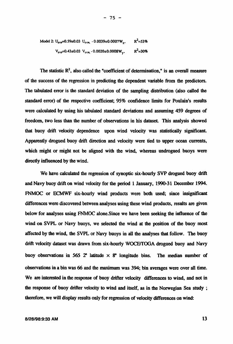
- 75 -

Model2: U5v..=O.S9±0.03 Us\"1'1 .. • 0.0039:t0.0007Wx• R2=53%

V5vv={).43:t0.03 V5,"1'L • 0.0020:t0.0008Wy• R2=30%

The statistic R2, also called the "coefficient of detennination," is an overall measure

of the success of the regression in predicting the dependent variable from the predictors.

The tabulated error is the standard deviation of the sampling distribution (also called the

standard error) of the respective coefficient; 95% confidence limits for Poulain's results

were calculated by using his tabulated standard deviations and assuming 459 degrees of

freedom, two less than the number of observations in his dataset This analysis showed

that buoy drift velocity dependence upon wind velocity was statistically significant.

Apparently drogued buoy drift direction and velocity were tied to upper ocean currents,

which might or might not be aligned with the wind, whereas undrogued buoys were

directly influenced by the wind.

We have calculated the regression of synoptic six-hourly SVP drogued buoy drift

and Navy buoy drift on wind velocity for the period 1 January, 1990-31 December 1994.

FNMOC or ECMWF six-hourly wind products were both used; since insignificant

differences were discovered between analyses using these wind products, results are given

below for analyses using FNMOC alone.Since we have been seeking the influence of the

wind on SVPL or Navy buoys, we selected the wind at the position of the buoy most

affected by the wind, the SVPL or Navy buoys in all the analyses that follow. The buoy

drift velocity dataset was drawn from six-hourly WOCF/fOGA drogued buoy and Navy

buoy observations in 565 ? latitude x SO longitude bins. The median number of

observations in a bin was 66 and the maximum was 394; bin averages were over all time.

We are interested in the response of buoy drifter velocity differences to wind, and not in

the response of buoy drifter velocity to wind and itself, as in the Norwegian Sea study ;

therefore, we will display results only for regression of velocity differences on wind:

8/28/98:9:33 AM 13

- 76 -

~AVY-Usvp=-0.0361±0.0144 + 0.0166±0.0029Wy•

VNAvv-V svp=-0.0148±0.0110 + 0.0145±0.0034Wx.

R2 = 9% df= 331 s=26

R2=5% df=357 s=21

We have included values for the degrees of freedom, df, and the standard deviation

of the residual, a. The former has been used to detennine the 95% confidence limits of the

regression coefficients. The percent of variance tabulated above is considerably less than

the percent of variance explained in the North Atlantic. Reasons to expect this are: buoy

observations in the 1-D analysis above were separated by up to 800 kilometers zonally,

200 kilometers meridionally and weeks in time. Additionally, the North Atlantic analysis

was restricted to 14° of latitude in the Arctic, whereas the SVP/Navy data ranged from the

tropics to f:lr N, and as we will show later that the relationship between the velocity

difference and wind is dependent on the Coriolis parameter. Fmally, when stricter

selection criteria were applied to the data and the binned means used in this analysis, the

percent of variance explained increased.

The same model was tested with the binned SVP and SVPL dataset; this dataset

was drawn from 3001 pairs of 'Z' latitude by SO longitude binned SVP and SVPL velocity

observations. The median number of observations in a bin was 75 and the maximum was

1679:

UsVPL-Usvr0-0009±0.0004 + 0.0135±0.0009Wx,

VSVPL-Vsvr0-0015±0.0034 +0.0120±0.0012Wy•

R2=13% df=l710 s= 1.5

R2=5% df=l835 s=14.

The percent of variance explained in this dataset by the first two models was very

nearly the same as explained in the SVP and Navy dataset. . The constant tenn evaluated. fa

zero within 95% confidence. Agreement· between the SVP/Navy Dataset ·and the

SVP/SVPL Dataset is good. The regression coefficient of buoy drift on wind velocity was

in agreement for any particular model regardless of dataset.

8/28/98:9:33 AM 14

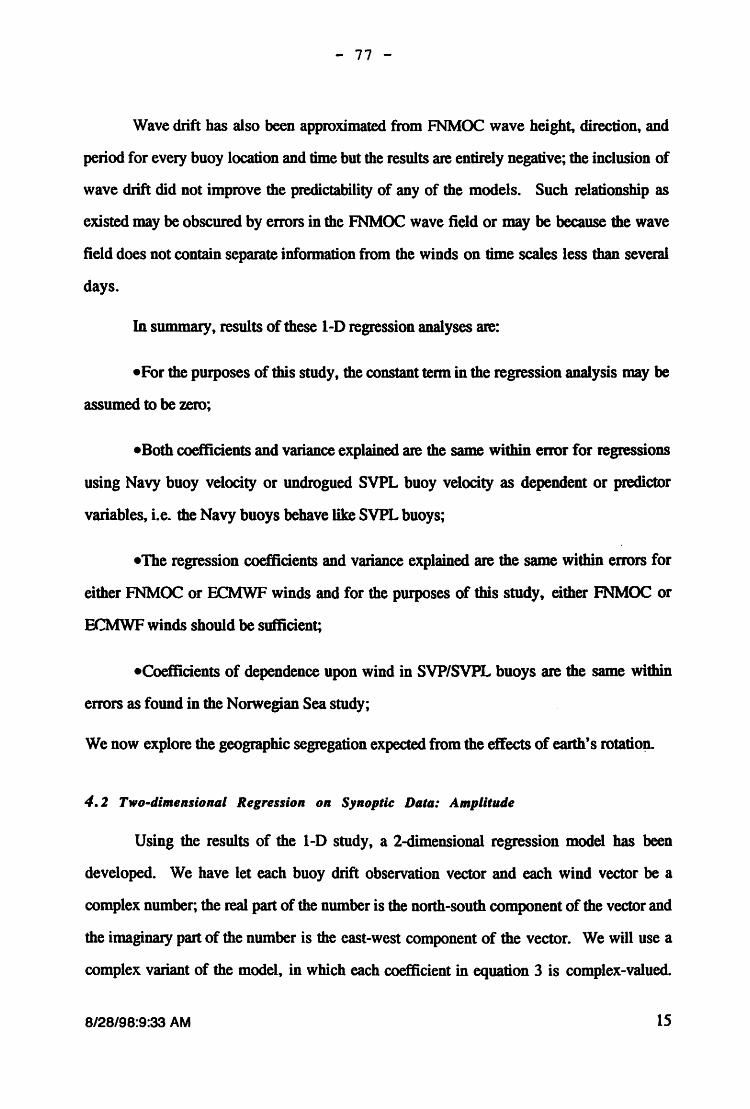
- 77 -

Wave drift has also been approximated from FNMOC wave height, direction, and

period for every buoy location and time but the results are entirely negative; the inclusion of

wave drift did not improve the predictability of any of the models. Such relationship as

existed may be obscured by errors in the FNMOC wave field or may be because the wave

field does not contain separate infonnation from the winds on time scales less than several

days.

In summary, results of these l-D regression analyses are:

• For the purposes of this study, the constant tenn in the regression analysis may be

assumed to be zero;

• Both coefficients and variance explained are the same within error for regressions

using Navy buoy velocity or undrogued SVPL buoy velocity as dependent or predictor

variables, i.e. the Navy buoys behave like SVPL buoys;

•The regression coefficients and variance explained are the same within errors for

either FNMOC or ECMWF winds and for the purposes of this study, either FNMOC or

ECMWF winds should be sufficient;

•Coefficients of dependence upon wind in SVP/SVPL buoys are the same within

errors as found in the Norwegian Sea study;

We now explore the geographic segregation expected from the effects of earth's rotatio~

4. 2 Two-dimensional Regression on Synoptic Data: Amplitude

Using the results of the 1-D study, a 2-dimensional regression model has been

developed. We have let each buoy drift observation vector and each wind vector be a

complex number; the real part of the number is the north-south component of the vector and

the imagiruuy part of the number is the east-west component of the vector. We will use a

complex variant of the model, in which each coefficient in equation 3 is complex-valued.

8/28/98:9:33 AM 15

- 78 -

Following the results of the 1-D study in the previous section, the coefficient A was set

equal to zero. Having confirmed the dependence of undrogued drift upon drogued drift in

the 1-D study, the regressions of undrogued(drogued) drift on drogued (undrogued) drift

were eliminated. The 2-d regression analyses were done on two scales; first, the data in

each ? latitude by SO longitude bin was used to calculate a regression of either six-hourly

synoptic drogued or six-hourly synoptic undrogued buoy drift on synoptic undrogued

wind:

UsvPL= BsvPL • WsvPL'

Usvp= BsvP • Wsvp

(4.1)

(4.2)

Since we have been seeking the influence of the wind on SVPL or Navy buoys, we

selected the wind at the position of the buoy most affected by the wind, SVPL or Navy.

However, the average wind at the position of the SVPL buoy was constrained to be within

1 m/s of the wind at the SVP buoy; results should be nearly independent of the choice of

wind, W svPL or W svp- The phase angle of the complex linear regression coefficient was the

angle of the response of the buoy drift to the wind.

In order to find the underlying relationship between the buoy drift and wind

forcing, it was necessary a priori to reduce the noise created by eddies and shears of strong

currents. From the many bins, 27 were found which met the following criteria:

• The wind should explain over 60% of the variance of the SVPL buoy drift,

e.g., there was a wind-driven circulation;

• The number of 5-day observations in a bin were ~least 15 or more;

• The percent of observations contributed by one buoy could not be more than

20% of the total. · The latter criterion was suggested by previous experience

with drifting buoy data analysis;

8/28/98:9:33 AM 16

- 79 -

• In rare instances where the SVP buoy drift was highly correlated with the wind

the velocity difference relationship is obscured - velocity difference becomes a

small difference between two large numbers - and these instances were also

rejected;

• Any instance of retrograde motion of an SVPL buoy was rejected on the

grounds that such a dynamics was unphysical and probably represented an error

in wind or buoy drift or both.

The distribution of these bins is displayed as open circles in Figure 3; the selected

bins were extra-tropical, ranging 1ff to nearly (:U in latitude away from the equator. The

number of observations/ bin in exceeded 15 and often exceeded 100. Each bin yielded an

estimate of the complex coefficient B of the vector regression equation using singular-value

decomposition and assuming a Gaussian normal error distribution for binned mean drifter

velocity differences: Since each bin extended over only ? of latitude, it was not necessary

for this equation to have a term which depends upon the latitude. As will be explained

later, the dependence on wind is best examined in terms of the phase and amplitude of the

complex coefficients, rather than the real and imaginary parts. The results of this analysis

are displayed in in terms of amplitude and phase of Bdifl'ereace rather than real and imaginary

components. Taking the difference of equation 4.1 and equation 4.2, we have:

Udlfl•r•nc•= USVPL- UsvPt

= Bdlfferenci WSVPD

ID I 'J.td)J 360 = r' d(ffereac~. e . WSVPL

(5)

The complex coefficient BdiffeteDCe is the difference between the coefficients B5v,.. and

BsVP. A is the phase of BdlfTereace in degrees. Figure 5 (bottom) displays a scatterplot of

amplitudes of Bdl«ereace vs. latitude for 27 selected bins; a least-squares best fit to a linear

Beman model of latibldinal variation of the amplitude of BcU«ereace explains 34% of the

8/28/98:9:33 AM 17

- 80 -

variance in Bdifference· The model is explained in the next section. Estimates of the 95%

confidence limits of Bdiffereac:e are shown in this figure; the mean confidence limit so

estimated is approximately 0.001 m/sec. We also computed the regression of binned mean

udiffereac:e on wind and a function of the Coriolis parameter, which solved the problem on a

global scale, instead of the sub-bin scale for which equation 4.1 and equation 4.2 were

solved as discussed above. Data was summarized by computing the mean and standard

deviation of buoy drift and wind, W, in the every bin; the first !-dimensional regression

results were derived from such summaries. The 2-dimensional analyses used similar

summaries, which differ in that buoy drift and wind were complex quantities. These

results explained over 47% of the variance in the amplitude of udiffereace if a tenn explaining

variability with the Coriolis parameter was included In order to explain these results more

completely it is now necessary to examine the nature of variability with the Coriolis

parameter in more detail.

4.3 Undrogued-Drogued Buoy Velocity Differences

Following the above analysis the equations for the latitudinal dependence of the

coefficient B in equation 5 can be rewritten:

( -112) 21dAJ360 w "difference= Bo + Bl. f . e . SVPL' (6.1)

(6.2)

. .

where udiffereac:e and WsvPL are complex valued, but all other parameters are real valued. . .

Observed amplitudes of B are plotted versus latitude in Figure 5 (bottom) and can be used

to solve for the amplitude of the coefficients in equation 6, assuming the complex phases

8/28/98:9:33 AM 18

- 81 -

(A.) of B0 and B1 are identical. This is essential since the theoretical analysis above bas

shown that A. varies inversely with the scale depth, and the scale depth is a linear function

of both the wind speed, W svPL' and the reciprocal of the square root of the Coriolis

parameter, f 112• Unear regression returns 8 0=-0.003 , 8 1=0.00016 (sec112

), where f is the

Coriolis parameter. There was evidence that the standard error of the coefficients returned

by this regression overestimates the error over much of the latitude range because the

envelope of points in Figure 5 (bottom) expands from lower to higher latitudes. Taking

this into account and disregarding five extreme outliers of 8, more than 3a from the model

curve of 8 derived from 8 0 and 8 1, above, the values of 8 converge to an amplitude of 2 at

2ff latitude and are enveloped by a lower curve (upper curve for absolute latitudes less

than Y) described by 8 0=-.017, 8 1=0.00026 (sec112) and an upper curve (lower curve for

absolute latitudes less than 2()0) described by 8 0=0.009, 8 1=0.00009 (sec112). The

envelope enclosed over 80% of the data and was used to make an estimate of co~dence

limits for the amplitude of the wind coefficient The difference in the lower and upper

bounds of the wind coefficient IBI defined the longitudinal axis of an error ellipse:

est= p.026- 0.00017· r1 '2 ~ ifest~ .1 e81 = .001; otherwise

(7)

fwis constrained by the mean 95% confidence limit on IBI values shown in Figure 5

(bottom). It follows that the longitudinal axis of the velocity difference error ellipse (along

the direction of Uo) was:

(8)

The error will be discussed further in Section 4.5, below.

8/28/98:9:33 AM 19

- 82 -

4. 4 Two-dimensional Regression on Binned Means: Amplitude

A regression was also made of binned mean drifter velocity difference on binned

mean buoy wind; this analysis assumes equation 6.1 and equation 6.2 held for mean buoy

drift and mean wind, just as it did for synoptic buoy drift and synoptic wind. A scatterplot

of the mean buoy velocity difference vs. the mean SVPL buoy wind for the same selected .

bins as .used in the analysis above is· shown in figure 5(top ); because no latitudinal

dependence is included, the plot shows a trend equivalent to a low absolute B-value of

0.87. Including latitudinal dependence would require a 3-dimensional graph; the complex

multiple regression equation is:

(9)

Solutions to equation 9 are limited because the complex B, and B1 coefficients in

this equation cannot reproduce the variation in A· which can be explained by equation 6.2 .

The full solution of equation 9 for binned means is displayed in Figure 5(bottom) as the

dashed line indicating the regression on binned means (A=O). As can be seen, the solution

is very close to the best fit to the regression coefficients computed frOm six-hourly .synoptic

data. As a check on the assumption of no constant term in equation 9, we have also plotted

the regression on binned means assuming A;f(). These-regressions explain over 47% of the

variance.

4. 5 Two-dimensional Regression: Angle of Response

The angle of response, A, of SVPL and Navy buoy drifter velocity. difference to

vector wind is shown in Figure 6. The angle· of response is the phase angle of the complex

B coefficient, given by

A.= ArcTan(lmaginary( B) /Real( B)), (10)

8/28/98:9:33 AM 20

- 83 -

For heuristic reasons, we have displayed the scatterplot of the response angle

derived from synoptic data vs. latitude in Figure 6 (top); no relationship can be seen

between the phase angle and latitude. However, as implied in the discussion in section

3.1, the angle depends upon both the Ekman depth and the inverse square-root of the

Coriolis parameter. The relationship in equation 2 suggested dependence of the response

angle upon the product of the wind and the reciprocal of the square root of the sine of the

latitude, shown in Figure 6 (bottom). This quantity, 1;, is proportional to the Ekman depth,

HE, defined in equation 2. Scatter is still great and the percent of variance explained in this

figure is low, but a Student's T -test shows that the ttend exists with greater tban 95%

confidence. Deviation from the trend in this figure may be because the relationship does

not hold under all ocean conditions. No clear estimate of the variation of the angle of

response with latitude could be obtained from the binned mean regression analyses; this is

not surprising since it is obvious this complex regression would only show a clear

relationship if there were a clear trend in Figure 6 (top). The best estimate of a fixCd angle

of response from this analysis is approximately 25°, in the middle of the range of observed

angles.

The range of the angles of response shown in Figure 6 at any latitude was 100; the

precision of this estimate could be improved but not the accuracy. The transverse axis of

the error ellipse for 8 is:

e,_. = o.l74S·IB ~ (11)

Therefore the transverse axis of the velocity difference error ellipse was:

(12)

8128198:9:33 AM 21

- 84 -

4. 6 The Most Likely Exponent of the Corlolis Parameter

As bas been discussed earlier we expect the buoy velocity difference to be

proportional to the reciprocal of the square-root of the Coriolis parameter. We have tested

the assumption that the exponent should be -112 and show the results in Figure 7. The

amplitude of the regression coefficients, IBI, obtained from the synoptic analyses are

modeled by the equation

(13)

where values of IBI were taken from the observed coefficients for selected bins

(section 4.2). Rearranging tenns and taking the natural logarithm of both sides of the

equation reveals a regression equation which can be solved for B and e:

In (B- B0 ) = In B1 + e In (sin (latitudq) • (14)

8 0 is set to -1, which is greater than its lower bound and the equation is solved for

e, a process equivalent to finding the best straight-line fit to the scatterplot in Figure 7 .. The

results indicated e=-.53 was an optimal fit

5. Model of Ekman Surface Current and Leeway Drift

5.1 Model Theory

The drift velocity of a SVPL or Navy buoy is composed of the wind forced leeway drift

plus the Ekman and geostrophic currents. ··Since' the geostrophic current can be taken

constant fro~ the ocean surface t9 _the. d~~ue. ~epth, the geostrophic co~nent of SVPL

or Navy buoy drift can be taken equal to the geostrophic component of SVP buoy drift and ... . .. )

~~oved from consideration. A plan view, of SW-and .. SVPL or Navy buoy drift vectors

are shown in Figure 8, in which wind is directed towards the top of the figure by

convention. In this figure the Ekman current vector of the SVPL or Navy buoy, Do" and

8/28/98:9:33 AM 22 ·' •.'·

- 85 -

of a buoy drogued at 15 m, u15, approximately have absolute value equal to (Ralph &

Niiler, 1998):

u_- U - fJu. --u- 15- J1' (15)

where the coefficient P parameterizes the effects of a vertical density gradient We use an

empirical expression for the friction velocity,

(16)

where Co is the stress drag coefficient, set equal to 1.2x10-3, P. is air density, Pw is water

density, and W is the wind velocity. The figure shows tbat the difference between SVPL

or Navy buoy drift and SVP buoy drift, the total buoy velocity difference, is equal to the

sum of the vectors .duE and Us· Leeway drift is parameterized by the coefficient, a, in an

expression which states tbat there is a drift of flotsam down wind,

Us=au. (17)

The FJanan velocity difference , .duE, is the vector difference between Do and u15• We

derive an expression for 4ue, starting with the geomettic identities:

(18.1)

(18.2)

(18.3)

8+48= Bo =8+~. (18.4)

8128198:9:33 AM 23

- 86 -

where ' = AB . The rotation, A9, of the Ekman current vector with depth is parameterized 2 .

by a constant 'Y (Ralph & Niiler, 1998):

AB= r z/z.o, (19)

Applying the definition of Zo as the scale depth !iJ. Combining 18.1 and 18.3 and

eliminating .Ao, then using 18.2 to eliminate A,:

(20)

where 6 + A9 = 90 by definition. Then by trigonometry and the above results, we find:

(21)

which implicitly relates AuE and lJs, and an expression for AuE:

(22)

For small ~' and using equation 15, this expression becomes

(23)

where ~ is here defined as yp2•

The line DB represents the total buoy drifter yelocity difference vector in Figure 8, identical

to the quantity udifrereac:e in equation 5. Using trigonometric identities to find BE and DE and .....

stimming these segments to find DB: ··

Buoy VelocityDiffert:nc~~;- udlfferellce= fluE co gp +au. coM. (24) .-· .... '

We:w_ill first demonstrate that ~erence .~s .a f.t:u:tcu~n~ of the parameters a, p, 'Y, and e()t and

then discover the statistically optimal values of these parameters in that order. By

B/28/98:9:33 AM

- 87 -

examination, equations 15, 22 and 23 determine the first term AuE to be a function of f, a,

P and 'Y (or~). When calculating values for AuE, l1w and fare detennined by the data and

values for· Co, Pa, and Pware selected from published values. The coefficients a, P and 'Y

are unknown and must be determined from the SVP and SVPL or Navy buoy drift data

The factor coscp must be calculated; using trigonometric identities, an expression for the

unknown «1» can be derived from equation 21. l; is proportional to 'Y by definition, making

«1» a function of e0 and y. The velocity difference angle , A, is implicidy determined by

equation 20 if the angles ct», ~, and e are known. Since e is a function of 'Y, eo and

observables, the assertion that ucHflema is a function of a, p, eo and 'Y alone is

demonstrated. Detennining the values of these parameters which minimize the model error,

(25)

is the object of our analysis. We used the same selected, binned, mean dalaset for the

analysis as was used in Section 4.

5.2 Mtnkl PtuiiiiUter Results

The flanan current vectors of SVP buoys in three typical ocean conditions are shown in the

left panel of Figure 9. The model equations, depending as they do on solutions of

equations containing ttanscendentals, so the model solution for udifCereace was determined

by implicitly solving equation 24 for optimal values of a, p, e0 andy, using the selected

datapoints shown in Figure 5 and discussed in Section 4. 2. The minimum variance of the

difference between the modelled values of Dcurrereace and the observed values of u.naereace' X2

'

was mapped against the unknowns. Since equation 23 suggests tbat the parameter ~

8128198:9:33 AM 2S

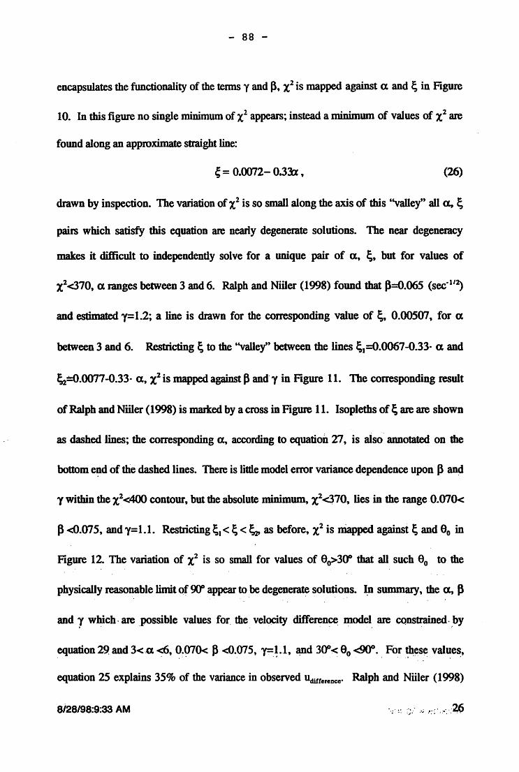
- 88 -

encapsulates the functionality of the tenns y and 1}, X2 is mapped against a. and ~ in Figure

10. In this figure no single minimum of X2 appears; instead a minimum of values of 1,2 are

found along an approximate straight line:

~ = 0.0072- 0.3lx ' (26)

drawn by inspection. The variation of '1} is so small along the axis of this ''valley" all a, l;

pairs which satisfy this equation are nearly degenerate solutions. The near degeneracy

makes it difficult to independently solve for a unique pair of a., ~, but for values of

X2<370, a. ranges between 3 and 6. Ralph and Niiler (1998) found that p=0.065 (sec- 11~

and estimated y=l.2; a line is drawn for the corresponding value of~, 0.00507, for a.

between 3 and 6. Restricting~ to the ''valley" between the lines ~1=0.0067-0.33· a. and

~=0.0077-0.33· a, X2 is mapped against I} and· y in Figure 11. The corresponding result

of Ralph and Niiler (1998) is marked by a cross in Figure 11. Isopleths of l; are are shown

as dashed lines; the corresponding a, according to equation 27, is aiso· annotated on the

bottom e~d of the dashed lines. There is little model error variance dependence upon f} and

1 within the X2<400 contour, but the absolute minimum, X2470, lies in the range 0.070<

p <0.075, and y=l.l. Restricting l;1 < l; <~as before, 1,2 is niapped against l; and 90 in

Figure 12. The variation of X2 is so small for values of 90>300 that all such 90 to the

physically reasonable limit of 9Cr appear to be degenerate solutions. ~ summary, the a, P . ' . . . .

and y w~ch. are .possible values for. the. velQCity differen~ ~odel. are CQns~ed. ,bY

equation 29 and 3<.a <6, 0.070< P <0.075, y=l.l, ~d 300< 90 <!JOO. For ~ese values, • • .·" • •• • ! • • ,, • • ..

equation 25 explains 35% of the variance in observed udifterence· Ralph and Niiler ( 1998)

8i28/98:9:33 AM

- 89 -

found that equation 15 explained 49% of the variance of U1s; given that We are attempting to

explain the variance of the difference of two velocities, ~i«ereace' not the variance of a single

velocity, u1 s, the lesser amount of variance explained is expected

Acknowledgements. This work has been supported by the Naval Research

Laboratory, contract N00014-95-C-6002. We wish to thank Harry Selsor, the corR for

this contract, deserves thanks for his constant encouragement and help. Thanks to Harley

Hurlburt, Charlie Barron Joseph Metzger, Steve Piacsek and Alex Wam-Vamas for

infonnative discussions. Thanks to Andre Bolduc (MEDS), Dennis Laws (FNMOC), and

Roy Lowry (Bidston UK) for their help with data issues. Thanks to Andy Sybrandy, Elise

Ralph, Sharon Lukas and Judy Gauke of SIO for their help with the SVP dataset.

REFERENCES

Caldwell, D., C. W. Van A~ and K. Holland, A laboratory study of the turbulent Ekman

boundary layer, Geophys. Fluid Dyn., 3, 123-160, 1972.

Chereskin, T ., 1995, Direct evidence for an Ekman balance in the California Current, J.

Geophys. Res., 100, 18261-18269.

Davis, R.E., Drifter observations of coastal swface currents during CODE: The statistical

and dynamical views, J. Geophys. Res., 9 0, 4756-4772, 1985.

Ekman, V. W., On the influence of the Earth's rotation on ocean-currents, Ark. Mat. Ast.

Fys., 2, 1-52, 1905.

Luther, D., A. Chave, J. filloux, and P. Spain, Evidence for local and non-local

barotropic responses to atmospheric forcing during 8~ Geophys. Res.

Letts., 1 7. 949-95~ 1990.

8128198:9:33 AM

- 90 -

McPhee, M.G.,.l995. On the turbulent mixing length in the ocean boundary layer, J.

Phys. Ocean., 2 4, 2014-2031.

Niiler, P.P., and E.B. Kraus. One-dimensional models of the upper ocean. In:

Modelling and Predication of the Upper Layers of the Ocean, edited by E.B.

Kraus. Pergamon Press, 1CJ77, pp. 143-172.

~iller, P.P., R.E. Davis; and H.J.White, 1987. Water-following characteristics of a

mixed-layer drifter. Deep-Sea Research, 3 4, 1867-1881.

Niiler, P.P., J.D. Paduan, A.L. Sybrandy and L. Sombardier, 1991. The WOCEfiOGA

Lagrangian surface drifter. Proceedings of Oceans 91, Hawaii, October 91, 839-

843.

N"Iiler, P.P., J. Filloux, W.liu, R.M. Samuelson, 1993. Wind forced variability of the

deep eastern North Pacific: Observations of sea floor pressure and abyssal currents.

J. Geophys. Res., 98, 22589-22602~

Niiler, P.P., A.L. Sybrandy, :K Bi, P. Poulain, and D. Bitterman, 1995. Measurements

of the water-following capability of holey-sock and TRIST AR drifters. Deep-Sea

Research, 4 2, No. 11/12: 1951-1964.

Pazan, S.E. and P.P. Niiler, 1998. Final report on Comparison ofDrogued and

Undrogued Drift Buoys, Naval Research Laboratory, Code 7406, Stennis Space

Center, MS 39529-5004. 51 pp.

Pedlosky, J., Geophysical Fluid Dynamics. New York:Springer-Verlag, 1982.623 pp.

Poulain, P.-M. and D.V.HUsen, 1996. Qllality'control and interpolation of

WoCF.rrooA drifter data. J. Atm.Oc.Tech. 13, 900-909.

PoulainJ».-M., A.. W~-v8mas, ~d P.P. Niner, t996. Near-surface cirCulation Of the

Noidic seas .as m~urCd by' taP.gian drif~rs •. JGR, fo l, No~· C8:' i8~37-

18,259.

8128198:9:33 AM

- 91 -

Ralph, E.A., and P.P. Niiler, Wind driven currents in the tropical Pacific, J. Phys. Ocean.,

in press, 1998.

Selsor, H.D., 1993. Data from the sea: Navy drift buoy program. Sea Technology.

December, 1993, 53-58.

Sybrandy, Andrew L. and Peam P. Niiler, 1991. The WOCEITOGASVP Lagrangian

drifter construction manual. La Jolla, Calif. : University of California, San

Diego, Scripps Institution of Oceanography, Scripps Institution of Oceanography

reference; 91-6,58 p.

8/28/98:9:33 AM 29

- 92 -

METOCEAN CMOD (AN/WSQ-6) DRIFfER

Figure 1 (right) AN/WSQ-6 drifter buoy design; this schematic is after ARGOS 61532, deployed February 9, 1992. Its manufacturer's designation is CMOD I, a multi-parameter, satellite reporting mini buoy series for Tactical Oceanographic Warfare Support. (from MEI'OCEAN Ltd.) CMOD II is much the same except for a larger flotation collar.

- 93 -

TECHNOCEAN LAGRANGIAN HOLEYSOCK DRIFrER

/ 0.20m

0.46m

Figure 1 (left) SVP Technocean Holeysock drifter buoy design; this is after ARGOS buoy 1425, deployed January 12, 1994. Note the enormous size of the drogue relative to that of the Metocean AN/WSQ-6 (CMOD). It has a subsurface float and Urethane carrots at all float-tether connections mediating the stress on the tether. The exploded 4x view of the swface float is included in order to enable a better intercomparison with other buoy schematics.

- 94 -

GLOBAL DRIFTING BUOY DATABASE 1988-1994

~00~--------------------------------~

= li1 i 30000

i s 20000 ~ ~

110000 • 0

0 1988 1990 1992

YEAR

1994

Figure 2. Global monthly summary of the number of drifting buoy observations per month in the Ocean Prospects data archive. The SVP and SVPL datasets are comprised of Lagrangian drifters deployed by the WOCFJTOGA scientific programs. Observations from a Lagrangian drifter are counted among the SVPL (undrogued) drifters after an on-board sensor indicates the buoy's drogue has been lost The Navy dataset is comprised of AN/WSQ-6 drifters.

- 95 -

DISTRil3UTION OF BINNED MEANS .AND REGRESSIONS

1 80oE LONGITUDE

Figure 3. Distribution of binned means and regressions where both SVPL or Navy buoy data and SVP buoy velocity data exist in a single 2° latitude by go longitude bin; selected bins are black circles (SVP/SVPL) and crosses (SVP/NA VY).

- 96 -

PROBABILITY DISTRIBUTION OF SVP /NAVY BUOY VELOCITY DIFFERENCES FROM MODEL

GO'N

~ 30'N ::J 1-

3 o· .. .-~-

/ /'

' I

• ·1.5 0.0 1.5

180'E LONGffi.JOE

90"W

N:IUoW. SCCRfS

o·

PROBABILITY DISTRIBUTION OF SVP/SVPL BUOY VELOCITY DIFFERENCES FROM MODEL

GO' N

~ 30'N

~ j

o·

180'E LONGm.DE

90'W o·

>-g (/) .5 m...J o<i w::J ::::~Q 8 [l 0 o::O:: 0 ...J t..s <i2 ~0 N

.•

·2 0.0 z IoCR loW. SCCRES

Figure 4. (RIGHT) The graph of residuals vs. the normal score statistic is a straight line if the assumption that the distribution of residuals from the regression are normal is true. (LEFT) Spatial distribution of 2° latitude by go longitude by 1 month summaries used in the regression analysis. Light shades denote regions where an anomalous relationship holds between wind and zonal SVP buoy drifter velocity.

0.15

........ (/)

' :E ._, 0.1 c UJ

~ (/)

- 97 -

DRIFTER VELOCITY DIFFERENCE VS. WIND SPEED

WIND SPEED (MIS)

REGRESSION COEFFICIENT vs.

LATITUDE

LATITUDE

~ Q ...

0

• SVP/SVPL

SVPINAVY

0 SVPISVPL

• SVPINAVY

B = 0.016*sin0atitudc)'•rz - 0.0026

REGRESSION ON BINNED MEANS (A::I) 8 = O.OlS*sin(latitudc)lrz

REGRESSION ON BINNED MEANS (.ul) B = 0.022*sin(ladtude)'lfl - 0.0011

Figure 5 (fOP) SVP/SVPL (circle) and SVP/Navy (diamond) buoy drifter velocity difference on wind; error bars are 95% confidence limits. (B01TOM) SVP/SVPL (circle) and SVP/Navy (diamond) regression coefficients of vector buoy drifter velocity difference on vector wind vs. latitude; error bars are 95% confidence limits. The model assumes an inverse square-root dependence upon the Coriolis parameter.

- 98 -

ANGLE OF RESPONSE DEPENDENCE ON LATITUDE

AP -0.078LATITUDEi- 28.0

LATITUDE

ANGLE OF RESPONSE DEPENDENCE ON SCALE DEPTH

0~----~~----~----~------~ 10 15 20 25

~-w. <sm (latitu de~12

0 SVP/SVPL

• SVPINAVY

0 SVP/SVPL

• SVPINAVY

Figure 6. SVP/SVPL (circle) and SVP/Navy (diamond) angle of response of vector buoy drifter velocity diff~ to vector wind vs. latitude; error bars are 95% confidence limits. The angle is left (right) of the wind in the northern (southern) hemisphere. There is no significant trend of A vs. latitude (top), but there is a significant trend of A vs. the scale depth ; (bottom) with 98% confidenre.

- 99 -

e = -o.53 N = 16 (14 degrees of freedom)

1.05 •• • ........ • 0 0.90 ~ • "0 m 0.75 • ....... .6

0.60 • • I I I

-0.90 -0.60

ln(sin(latitude))

Figure 7. Given observed regression coefficients, B, of difference velocity on wind at different latitudes, the least-squares solution for the exponent of sin(latitude) is -0.53, supporting the choice of an exponent of -1/2 in the difference velocity model.

- 100 -

~ w ,,ol

1\ Figure 8. SVPL (undrogued) buoy drift, u.., and SVP (drogued) buoy drift at 15m. depth, U1, relative to the wind vector, W. The buoy drift difference vector, Do. is the vector difference U15 - Du· The SVPL drift vector is the vector sum of the Ekman drift, ~' and the

leeway drift, u,. A is the difference velocity drift response angle with respect to the wind.

- 101 -

~~ DAFTER I:A:);UEO AT 1S MCEPTH

UtDOGUED· ao:;UED mfT VB.oart DFFEI&CES

&~---=~--~~~--~ ·~----------------~

I I

I u.

)-

t:

8 I ..J

~ I

~ il-0

~ A ~

Q Z' i

~ c

J.. ~ -~ ~.L CRX&WNl HORW' llRllillDYVB.a:ITY

Figure 9. Buoy drift nonnalized by the Ekman velocity scale in three extreme upper ocean states representing the range of validity of the model: A. Ekman depth of 1OOm, strong winds very close to the equator; B. Ekman depth of 30 m, strong winds at high latitudes; C. Ekman depth of 15m, weak winds in the tropics. (LEFT) normalized Ekman velocity, u15, displaying the range of rotations with respect to the wind; (MIDDLE) the SVPL buoy velocity is a summation of surface layer Ekman velocity, tJo, and along wind leeway drift, Us; (RIGHf) total difference, Dt, between SVPL (undrogued) and SVP (drogued) buoy drift.

' \ I \

- 102 -

0.007 ----------------------------.,

X X

X X

• • • • ~ (sec-1)

X X

X

• • • • •

Figure 10. Error variance as a function of model parameters. The straight dashed line, ~=.0072-.32a, follows the minimum in the model error variance. The parameter ~ is defined as the product of the model prameters, yp2• The horizontal line in the lower left is

the range of~' a from Ralph & Niiler, 1998.

1.4

13

L2

1

- 103 -

DEPENDENCE OF MODEL ERROR VARIANCE ON MODEL PARAMETERS

\ ' ' • (X)55 . aJ8=( . CfJ£6

\ ' \ \ \ \ \ \ \ \

\ .aJ7

\ \ \ \ x\

\ \ \ \ \ \

\ \ \

600

\ \ \ \

\ \ \ \ \ \ ~ \ X\

\ \ \ \ .tc5 \ \ \\

~ '400

\ \

\ \ \ \ \

\ \ \ \ \ \ \ \ \

_ _.... ...... _\ X\ \\ X

\ \ \ \ \\ \

\ \

\ \ \ \ 40d\ \\ \ '\

\ \

\

\ \ '\ \ \ \ '\ X\ \ X \

\ \

\ \

' ' ' \ \ ' \ ' \ ' " \ ' \ \ \

X

X

\ \ \ ' \ \ \ \ X \.6,•7 \'\.X '\. X '\2.1

_, 62 3.7&:01 \ \ ' \ \ "

\ '\ ' \ \ \

\ ' ' '\ ' ~~--------------~--~----~--~----_.--~--~~--~

~ 0

~ (sec-1rl) Figure 11. Model error variance, X2

, near the dashed line in Figure 10; isopleths of l; are shown as dashed lines here. Derived values of a are assigned to each isopleth (see text). The cross ( +) is located at a reported value of P and 'Y (Ralph & Niiler, 1998). There is

little model error variance dependence upon P and 'Y for X2<400.

- 104 -

DEPENDENCE OF MODEL ERROR VARIANCE ON9o o.a:n

-~- ~ ....... X ' X X X

--~ ~ ' .,.. -..

" I ' ' ) I ( ' _?./ I ~ I ~ ' ~ I " ./

I \ ' / X X '

X x, I I

400 375 ' 450 425 \ ....... Q(X)S

I lx \ X X X

\ ( (

~ (sec-1) \ ' \ X

~ X ....... X X

'"" - - ~ ""._ -... X ' X X

' - .,.J

X ./ X 'X ./

' ' '\. \.

' ~ - "' ' ~

X X "'

X QCDS / ., _, _, -- ~ /" -- X X X X

\ .......

' X x, X X

'-

' "" " ~ ....... ~ ....... ........

QCD4

2~ 5(7

So

Figure 12. Model error variance as a function of 80 and ~ near the optimal values of a, P and y. Gradients in model error variance is small but there is a slight tendency towards larger9o-

'-"'

-

""" 7~

- 105 -

able 1. Drag area ratio of the AN/WSQ-6 (CMOD-11 variant) (from data supplied by ETOCEAN Data Systems) and rag area ratio of the TOGA/WOCE SVP Lagrangian Drifter (from iiler et al., 1991 ). rtier models of the AN/WSQ-6 buoy had a smaller float collar, frontal area, and therefore

aF1 er dra ratio.

ull loatation Collar

R H-30 fish netting ether

60.6 19

UNKNOWN 400

10.2 35.5

0.5

618 674

200

0.471 0.47

1.4

91.45 12.4 1134 0.4-1.0

tio of Drogue Drag Area to ether Ora Area rag area ratio of the TOGA/WOCE SVP Lagrangian Drifter (from iiler et al., 1991 ) urface Float n/a 34.29 923.5 0.47 ubsurface Float n/a 20.32 324.3 0.47 rethane below Surface Float 40 n/a 220.3 1 rethane above Subsurface Float 25 n/a 220.3 1 rethane below Subsurface Float 40 3.81 152.4 1 mall Hydraulic Hose 163.6 1.49 243.8 1.4 ether 856.06 . 0.56 475.6 1.4

rogue Section: rethane above Drogue rogue

tio of Drogue Area to Tether ra Area

40 644

4/-4 92

161/5 59248

1 1.4

38

- 107 -

Development of a Drifting Buoy Metadata File at the Global Drifter Center John Stadler Atlantic Oceanographic and Meteorological Laboratory (OAR/NOAA) U.S.A.

ABSTRACT ONLY SUBMITTED

The Global Drifter Center at the Atlantic Oceanographic and Meteorological Laboratory maintains a database on drifting buoys deployed worldwide. The metadata component of this database includes technical specifications, program information, deployment information and shipping history, for more than 5200 drifting buoys. Historically, this metadata included drifting buoys of many different designs, and maintenance of the information was inconsistent During the past year, a concerted effort has been made to update the metadata and fill in gaps in the data. Several significant changes have been made in the way in which the metadata is maintained: 1) the metadata was redesigned to take advantage of the relational capabilities of the software being used, resulting in a more compact database; 2) a unique identification number was created for each drifter; 3) criteria were established for inclusion of new drifters into the metadata; and 4) a standardized specification sheet, to be filled out by the manufacturer, was developed to provide a complete technical description of each new drifter. The goal of this presentation is to provide an overview of the structure of the metadata and the types of data that it contains.

- 109 -

Preliminary analysis of Ar2os 2 on NOAA K pertormanC'es

M. Taillade CLS I Service Argos

taillade@cls.cnes.fr

1. Space segment status and performance

1.1. Status

Fi~e 1 shows the status of the Argos space segment: - before May 1998, data wer~J~rocessed m global and regional mode from three satellites ~-NOAA 14 and 12 operational, NOAA 11 as backur third satellite), data from NOAA 10 being received from loca user terminals (LUTs) only; - between May and December 1st 1998, Oa.ta werMrocessed in 2lobal and regional mode from four satellites OAA 15 unaertest NOAA 14 and 12 operational, NOAA 1 as backlli> third satellite), data from NOAA 10 being received from ~UTs only· - from December 1st 1998, data will again be :Qrocessed in global and regional mode from three satellites (NOAA 15 and 14 operational, NOAA 12 as backup third satellite), data from NOAA 10 and 11 being received from LUTs only.

Satellite status Before After May98 December 1st 98

Under Test 15NOAAK

Operational 14- NOAA J 14-NOAAJ 15 NOAA K 12-NOAAD 12- NOAA D 14- NOAAJ

Back up Third satellite 11- NOAA H 11- NOAA H 12- NOAA D

10- NOAAG 10-NOAAG 11- NOAA H 10-NOAAG

Decornmissioned 9- NOAA F 9- NOAA F 9 -NOAAF

figure 1: Argos space segment status

- 110 -

1.2. Data collection performance Performance in terms. of passes per day and with respect to latitude for two-, three- and four-satellite service is shown in figure 2 below.

Number of Satellite passes per day

Latitude of the transmitter Mean number of passes per 24 hours in degrees with 2 satellites with 3 satellites with 4

satellites

0 7 10 14

±15 8 12 16

±30 9 13 18

±45 11 16 22

±55 16 24 32

±65 22 33 44

±75 28 42 56

±90 28 42 56

The number of satellite passes depends on the latitude of the transmitter

figure 3: Data collection performances

1.3. Data collection processing performance

Figure 3 shows the total messages received by each satellite from each orbitography beacon ourin_g August 1998. Results v~ by a few P-er cent from one satellite to another. Thts confirms that whatever the mode-under test, operational or backup-the four satellites offer similar data collection processing performance.

,_ 111 -

Nb of messages per month 15 12 11 14 15 12 11 14

PTT ID K D H J K D H

117 2979 2952 2976 3051 1% 1% 3% 110 3800 3788 3884 3980 0% 3% 5% 119 5278 5274 5423 5721 0% 3% 8% 111 3474 3488 3596 3459 0% 3% -1 % 108 5699 5765 5789 5929 -1 % 0% 3% 1 3397 3450 3484 3563 . -2% 1% 3% 118 3766 3874 3760 4252 -3% -3% 10% 109 2788 2899 2693 3108 -4% -7% 7% 149 2719 2838 2644 2934 -4% -7% 3% 112 3961 4137 3961 4250 -4% -4% 3%

Total 37861 38465 38210 40247 -2% -1% 5 figure 4: Data collection processing performances for orbitography platforms

2. Second-generation Argos instrument NOAAK was launched in May 1998 canyingArgos 2, the first second-generation Argos instrument. The mam enhancements to this new instrument are: - more receivin\channels (increased from four to eigh8; - wider receiver andwidth (increased from 24kHz to 8 kHz -see figure 4); - greater receiver sensitivity (increased by 2 dB).

~-... ·~

·· ''· 30kHz·.

High data-rate transmitters

4,5 kbits/s

ARGOS 3 110kHz

~ ARGOS 1 .... .. ~. . . 24kHz·

First-generation transmitters

400 bits/s

Low power transmitters

400 bits/s

tigure 4: Argos 1, Argos 2 and Argos 3 receiver bandwith comparison

~ > 0

..0 co: N ...... l..o ~ -....

- 112 -

These enhancements have brought two main improvements for users over the Argos 1 instrument: - a) more transmitters (PTTs) are within view of a satellite at any one time (factor-of-three-to-four increase); - b) messages are more easily received from low-power PTTs, and more messages can be received from a single PTT.

3. Increased receiving capacity

90000

80000

70000

60000

50000

40000

30000

20000

10000

0

3.1 . Current situation

•

Figure 5 shows the Argos 2 frequency band occupation during the satellites' 10 ~ -minute orbit period (each point on the grapli re~resents a received message). AllmessagesarewithintheArgos 1 band, i.e., 12kHzeitherside of 401.650 MHz. We should note: -That the group ofPTTs belonging to the Brazilianprogram is operating m the Argos 2 band with the Brazilian SCD 1 satellite and Argos 2. These two spa~e systems are compa_tible. -The curve of messages received by test PTT N° 1 m Toulouse, · France (see paragrapb .. . ).

Frequency band occupation during

••

• • •

• • • •

1000 2000 3000 4000 5000 6000 7000

se-

figure 5: Current frequency band occupation during an Argos 2 orbit

- 113 -

3.2.Capacity verification

0

Figure 6 shows occupation in the Argos 2 band for a satellite pass within view from Toulouse (lasting about 800 seconds) with a number of PTTs simulating Argos 2's maximum expected capactty.

200 400 600 800 1000

secondcs

figure6: Simulation of Argos 2 maximum occupation in visibility of Toulouse

This simulation is based on a transmitter and a P.rocessor that generates a set of virtual PTTs that behave like real PTTs during a satellite _pass. Analysis fOcused on the number of messages transmitted by the simulat9r and received by the location system (satellite and Q_rocesstng). This analysis showed that Argos 2 technical operating specifications were satisfied under maximum load.

1200

- 114 -

3.3. Strategy for widening range of PIT frequencies in the Argos 2 band 3.4. Test Two Argos transmitters were activated during NOAAK passes. The transmitters could send the same number of messages simultaneously--one operating in the Argos 1 frequency bancl the other in the Argos 2 bano-using the same power and repetition period. Message content was identical in each case.

Power Transm. power dBm

2 watts 33 31

1 watt 30 500mW 27 500mW 27

26

Transmitter 1 Received msg nb.

90 94 115 59 119 274

Inside Argos 1 Bandwith

Transmitter 2 Received msg nb.

99 104 132 110 182 414

Outside Argos 1

Band with

table 7: Transmission tests during NOAA K passes

Messages nb. difference

10% 11% 15% 86% 53% 51%

Table 7 (transmission tes~ during NOAA K p3;5ses) spo~s the . number of messages received from each transnntter, with signal ~9wers varying from 500 milliwatts to two watts. The last column shows the difference, in per cent, in number of messages received. . These results demonstrate that low-_power PTTs work better transmitting in a clear frequency bancf (here Argos 2) than when they share the same band with many other, mo~e _pgwerful PTTs all operating at the same frequency (401.650 MHz). 3.5. Approach These results support the approach decided by the Argos Operations Committee in Ancliorage in July 1998:

"The Argos Operations Committee, recognizing the need to optimize the use of the frequency bandwidth currently allocated to the Argos System (401.650 MHz +/-12kHz) resolves: - that the central frequency to be used by future A._!.-gos Data Collection Platforms be 401.650 MHz, 401.648 MHz and 401.652 MHz. All three frequencies being egually used, - that CLS shall take the necessary measures fur manufacturers to develoQ_ corresQonding Argos DCPs, - that CLS shoulo undertake the necessary studies to further optimiz~, the utilization of the band allocated to the Argos System.

- 115 -

4. Argos 11 Argos 2 comparative sensitivity analysis

4.1. Principle To analyze sensitivity, we need to compare PTT performance ~hen transmitting to satellites flying Argos 2 and Argos 1 mstruments. Unfortunately, a PTT is never in the same position relative to the satellite during each successive pass, so si~al attenuation is well above tlie difference in sensitivity (2 dB) normally ~bserved between the two instruments under laboratory condi­tions. To eliminate propagation errors and thus be able to analyze the performance of each satellite when receiving from the same PTT, we compiled a list of parameters for eacli PTT active over a one-month period (see table 8- some of these parameters will serve to re:firie our analysis later).

IList of parameters for each platform

Platform data Platform ID number Programm ID number Program name Type of processing (loc123, loc 1230, .... ,data collection.) Type of Service (Standard, Limited, Back up) Repetition period Type of platform (marine, terrestrial animal, bird, buoy ... ) Platform latitude Platform longitude

General data collection performances Monthly total number of day with data collection for all satellites Monthly total number of passes with data collection for all satellites

Data collection performances for satellite (i) Satellite identification (i) Monthly total number of day with data collection for satellite (i) Monthly total number of passes with data collection for satellite (i) Monthly total number of passes with location for satellite (i) Monthly total number of messages for satellite (i) Monthly mean number of message per pass for satellite (i)

table 8: List of parameters compiled each month for each platform

- 116 -

4.2. Theoretical visibility Our analysis is based on a PIT located at a latitude of 45°. Satellite );?asses with an elevation angle of under 3 ° were eliminatea. Using real orbit parameter data, we calculated the theoretical total time each satellite was within view of the PTf during the month. Results are given in the table 9 below.

K D H J Satellites NOAA 15 NOAA 12 NOAA 11 NOAA 14

Visibilite cumulee (Heure) 32:10:49 32:12:11 33:52:25 34:00:40

-0,07% 5,19% 5,61%

table 9: Platform visibility theoretical total time from each satellite

NOAA 11 and 14 are nearly 20 kilometers higher, and their total visibility is 5% better than NOAA 12 and 15. · Plese ffgtJJes giye us some .idea oftpe d~~e.e.oftheoretical error Introduced by differences In satellite vtstbthty. ·

4.3. Satellite petformance .. We comp!J.fed the performance of satellites D~_J and H to that of NOAA K, on the basis of the mean numoer of messages received per pass by each satellite from the same. PTT dunng August 1998. ·

This parameter is a very ggod indicator of system performance, because it significantly affects both data collection and location results (at least four messages must be received during a pass to attempt type 1, 2, 3 or 0 location, at least three for type A. location, and at least two for type B location).·

4.4. Orbitography beacon performance The orbit~aphy network comprises high-power beacons that offer a ht level of performance. Because ese beacons are more powerful,., the mean number of messages received per pass by each satellite is not a significant indicator of sensitivity. However, results do give an overall indication of performance with a uniform set of reference beacons.

- 117 -

Table .. shows for each orbitography beacon: - the mean number Ni of messages received per pass by each satellite (i) during August 1998; -the difference in per cent between satellites K and D, K and H, and K and J, where:

d(K-j) = (NK-Ni)/Ni fori= D, H, J. ·

Orbitography 12 11 14 15 platforms IDs D H J K d(K-D) d(K-H) d(K-J)

Nd Nh NJ Nk

Canberra 11 2 23,3 23,8 23,8 23,3 0% -2% -2% ? 11 7 21,5 22,7 22,5 23,2 7% 2o/o 3o/o Hartbees 1 1 1 22,5 22,8 22,5 22,0 -2 o/o -3% -2% Kuerguelen 11 9 21,9 22,7 22,9 22,0 0% -3% -4% Mojave 11 0 22,2 21,4 23,0 21,2 -5% -1% -8% Kourou 109 21,5 19,5 22,0 20,4 -5% 5% -7% Wallops 11 8 21,4 20,3 21,9 19,6 -9% -3% -10% Gilmore 1 0 8 18,1 18,3 18,8 17,8 -1% -3% -5% Toulouse 1 18,0 17,5 18,4 17,0 -6% -3% -8% Perth 149 17,2 16,5 17,1 16,3 -6% -1% -5%

Total 208 205 213 203 -2% -1 0,4 -5%

table 10: Mean number of messages received per pass from orbitography network

The difference in the mean number of messages received ~er pass does not exceed 1 0% from one satellite to another over the entire network. As expected, these results show that NOAA K generally does not provide better performance than the other satellites with high­powerPTTs.

- 118 -

5. Analysis based on low-power PTTs Here, our analysis covered a set of303 bird-tracking transmitters 9_Qerating with three satellites during August 1998. We only considered PTTs for which messages were received from at least 24 passes during the month (thus eliminating transmitters yielding abnormal results).

5.1. Analysis of d(K-j) as a function ofPTI latitude

We plotted the parameters d(K-D), d(K-H) and d~-J)·on the figures 11 ,12 and 13. These parameters measure the _Qerfor­mance of each satellite in comparison with NOAA K as a function of latitude. ·

We can see from these curves that: - performance is a_pparently unaffected by PTT latitude; - results are significantly better with NOAA K, i.e., Argos 2 as opposed to Argos 1 on NOAA D, J and H. ·

J.. : • :. I ••• , : ...... . . ..... l .................. •-4-o ,-o . .

: . ~· ! •

• . • • • • • • • • •••.••••• 2'() ,-o

........ ~ ........ 4 ..

; .. :·• . . . . •••• • • • • • .. .A.... . . . • •· . • '! ............ :. : . ; ..... ....... . . . .. . . . :~ :. . '· : . .. . : : . ~ . .. . . . . .

. ... :•-.:- -~-~--. ··~- ........ : .....•.. : ........ -~ ......... : ........ . . . . . . . . . .;··-- . . . v: ~ • ; : : • . ~-·-. !.! .. ~ ......... ~ ......... : ......... ~ ........ -~ ......... : .. '~ ..... · . ••

- - - -· .. - •••••• - .: • - - • - •••• J .. - ••••••• .:. .......... - - - ... - - - - - - .. - .. ·- - - - ••••• -·- - - - - ••• - •

I t • t 1

· ................ ; .................. ~ ......... :. ......... : ......... . Mean number of messages per pass .. Difference between K and J

table 11: K (Argos 2) and J (Argos 1) comparison for low power platforms function of latitude

- 119 -

"'"'•'-' •• • • • •·I• .. : • • . _.,.~~···· ... : . :

. • 60~·~a~J' ; • • : •

. . . ~· ~ ···~··... . .. . . ' ----------------~t----~-----.40~~~:t:!.£.:; .. ~--~-------~~--i .... : ....... ~----

• ~J ~. .... • • : • • • . ~. . . ' • • • • • • • • • • • • • • • • • • • :· • • • • • • • • • • • • • 20 ~~ I ~ •• • • •• • • • • • • • • • • -. • • • • • • • • • • • • • • • • • • • .. • • • • • • • • • • • • • • • • • • • •

' . .

-50% • . , 0~ . 50%

. 100% • 15)%

-20,0•

. ' ... -.- •.. -.---- ••• ·:--.- ..... ---·4~ ............... --- .•• ---.-- ••• -.-.- ~-- _._ ••• --.-- •• --.- •

....... ... mean number of messages per pass • difference between K and D

table 12: K (Argos 2) and D (Argos 1) comparison for low power platforms function of latitude :.. . .......... . ' . . .. ... . . . . . .

~- ...... ;~- .... ~~~i ~t:P~: ... ~~~- .. ---:- -.-~- .. ;--·:·. -~- ....... -:-- ...... . •. • .. ·-4~~~ ···~·· • . • . . . • . . ,.. ~ ..... ' ' .. ' .......... ~· ... ' :· ' ·- · · ----;--- ---- -4eie .. ~ ·'W;.f---- -•r- ·•-- :¥- •• ·- • .. ~ ···--- · ·: • • • ·- -- :----- ·-- -:· ·-------... :.~ ...... :. . : . ' . . .. ' . . . . '

: ... : . : : : : : • • • .... •; • ...... ·28i8"~ .. • .,. -# .• Y., •••• • •. • ., •• • • • • • • • r • • • • • • • • • • • • • • ·- • .. • • • • • • • • .,. • • • • • • • •

• ... . :. : :

-5 )% 1SP%

. . . . . ' . • I I I t I I

· · · · · · -· ~ · -· ----.zo; a .. . -- -~- - ----.. -·- -.... -.. ~- --.. ---. ~ . -. -- --- ~ .... - .. - - ~ . -----.. -~- -- -.. -- -

···--····-•---~0 ... 1 ......... •-:·•-... ·--··•····•···-~·-·-····~·-····--~---······ . .

..........

Mean number of messages per pass - Difference between K and H

table 13: K (Argos 2) and H (Argos 1) comparison for low power platforms function of latitude

c ca G)

==

- 120 -

5.2. Analysis of d(K-i) as a function of number of P1Ts

90%

-20%

-30%

-40%

-50%

5.2.1. Analysis To plot curves 14 we:

a) created a three-column table for each {K- i) P-air; b) entered values of d(K- i) in decreasmg oraer in the first column; · c) entered the corresponding cumulative number ofPTTs in the second col~ starting with the highest d(K- i) values; d) converted this number into a percentage of the full set ofPTTs in the third column. Curves 14 allow us to compare the performance of Argos 2 (on NOAAK) and Argos 1 (on the other satellites) directly in terms of mean number of messages per pass.

. . . . . . . - • - ... - • - • - - .. - ........... - -·- - • - ••• - - , .. - - - - ..... -r - - - • - - .. - • - - - - - - - - .. - - - - - - - - •••• - - - - - - - ~ - - • - - - - -

I I I I I 0 0 I 41

. . .. : ........ ~ ........ ·:· ........ ~ . --..... ~ .. -.... - ~ ... --... ~ .. -..... -:· ..... --. ~ .. -.... . . . . . . . . .

- . -- --.. -- .. -.. -- - .. - . ------··- .... -- .. --- -- ........ -- -- .. ---... ---------- ---- .. ---·- ... -- ----.. - -- - -- .. -1 1 I I I I ' I I

I t I I 1 I I

- .. - - - - - ~ ........ - ••• - - - - - • - ••••• - - - - - .. ~ - - - ••• - - •• - - - .... - 4 - • - - - - - - -·- - - - - - - - - ._ - - - - - - - -

1 1 1 1 I I I

I I I t I I I ··-···········---------------············--·-··········----- --------·-·-········ . . . . Difference between K and J :

- - - - - •• - f ••••• - ... -........... ·,· - ....... - -.- - • - ....... t' - ... - ..... ~ • - .. - ..... ., - • - - - - - - -.· - • - - •• - • - •. • -

1 1 I f I I I

I I I I I o• f

-·······-·······························-····----·······--·······----------·------ -----• I I I . .

Cumulative number of platforms in %

figure 14: Argos 2 on K sensitivity compared to Argos 1 on H, D and J

- 121 -

6 Preliminary results

We can conclude from this preliminary study on a set of low­power PTTs thatArgos 2 performs better than Argos 1 with 70% of transmitters in tlie sample (70% with respect to NOAA H, 80% with respect to NOAA D and 85% with respect to NOAA

BOmparative values for each transmitter and each satellite with respect to NOAA K are given by curves 14.

For e?'ample, we can see that the mean number of messages per pass mcreases by:

- at least 50% for 10% of transmitters; -35% for 20% of transmitters; - and 10% for 50% of transmitters.

This s~dy should be pursued as soon as NOAA K switches to operational status.

By having a larger data set of platforms we should then be able to explore:

- why PTT performance varies from one satellite to another; - why some transmitters perform less well; - how far location accuracy improves; - variations in location classes; - performance with other types of transmitter samples.

- 123 -

Interactive Real-time Quality Control of Surface Marine Data at the National Centers for Environmental Prediction

Christine M. Caruso

National Oceanic and Atmospheric Administration National Weather Service (NWS}

National Centers for Environmental Prediction (NCEP) NCEP Central Operations (NCO} Camp Springs, Maryland, USA

1. Introduction

The accuracy of numerical prediction models which produce meteorological and oceanographic forecasts are dependent on; (1) the models• skill at sufficiently describing the physics of the atmo­sphere/ocean, and (2} the quality and quantity of the data used in their analyses and initializations. Al­though ever increasing numbers of marine observa­tions are being transmitted, the ocean observing network for providing operational measurements on a routine basis is still very sparse both spatially and temporally when compared to observations over land. Therefore, considerable effort is made to quality control (QC) those available surface synoptic observa­tions over the oceans. These quality-assured data must also be delivered to the numerical prediction models in a timely manner in order to be useful.

National weather and oceanographic centers are faced with two tasks which greatly affect their marine operations; ( 1) the time-critical QC of marine observations available for ingestion into numerical prediction models, and (2) the timely dissemination of both the QC'ed data and the forecast guidance based on the output from these numerical models (Richardson and Feit, 1990). This paper describes the Quality Improvement Performance System (QUIPS) being used by the NWS/NCEP!Marine Prediction Center (MPC) for the real-time QC of global surface marine observa­tions collected by ships, buoys, and Coastal Marine Automated Network (CMAN) stations. Also described are the next-generation interactive QC system cur­rently under development by NCO and the importance of buoy observations to weather forecasting.

2. Background

QUIPS was developed in 1987 by Compass Systems, Inc. for the National Ocean Service's Ocean Products Branch (OPB). The first version of QUIPS only allowed for the QC of sea-level pressure (SLP) reported by ships, moored and drifting buoys, and

CMAN stations. This version ran on a Micro VAX 3100 workstation using the VMS operating system. The ability to QC air temperature (AT), wind direction and speed (WD and WS), and sea surface temperature (SST) was added into the second version of QUIPS in 1991, and the software was moved to a VAX.station 4000 workstation, also running under VMS. Using QUIPS, OPB meteorologists performed real-time QC of all surface marine data received from ships, moored and drifting buoys, and CMAN stations. In October 1995, OPB was disestablished and the QC function, including personnel, hardware, and software, was transferred to the NWS. The meteorologists who perform the real-time QC are employed by MPC and the QUIPS software and hardware are maintained by NCO.

3. Data Collection, Coverage, and Use

Conventional surface marine data reported by ships, moored and drifting buoys, and CMAN stations are transmitted to NCEP via radio, satellite, and the Global Telecommunications System (GTS). In addi­tion, observations from the Navy and Coast Guard are sent via the Automated Weather Network. These data are used by MPC and NWS field office meteorologists and by NWS numerical models to produce analyses and forecasts. The data are also used to validate satellite-derived measurements and are used in climate and global change studies. Upon arrival at NCEP, the raw bulletins containing surface marine data are decoded and stored into BUFR (Binary Universal Form for the Representation of meteorological data) format files on NWS Cray supercomputers.

The spatial and temporal coverage of the existing conventional ocean network is sparse when compared to equivalent measurements over land (Waters et al., 1993). Additional marine platforms have increased the number of observations received, and the number of observations which may be stored in the NWS database has increased, so that the number of surface marine observations stored each month has

- 124 -

risen from 140,000 observations in 1993 to 355,000 observations in 1998 (these numbers don't include duplicate observations or observations from ships identified by the callsign 'SHIP'). However, the additional observations are primarily seen in the North Atlantic and North Pacific Oceans, and many of the drifting buoys reports only include SST measurements. With the exception of observations from ATLAS buoys moored in the tropical Pacific, all surface marine reports must include a sea-level or surface pressure observation in order to be assimilated by NWS' s Global Data Assimilation System (GDAS). A standard atmosphere pressure of 1013.25 mb is attached to reports from ATLAS buoys so that other measured parameters from these buoys may be used by NWS assimilation schemes and numerical models. Reports that include SST only are used in production of a one­week SST analysis which is updated daily and pro­duced by the Climate Modeling Branch of NCEP's Environmental Modeling Center (Reynolds and Smith, 1994). This SST analysis is used to provide boundary conditions to NWS's Aviation (A VN)/Medium Range Forecast (MRF) model.

4. Surface Data QC

Given the sparse nature of surface marine data, every effort must be made to ensure that these data will be used by the NWS assimilation schemes and numerical models. The accuracy of surface marine reports must also be known if marine forecast­ers are to produce accurate analyses and forecasts. As such, considerable effort is made to QC surface marine data. MPC meteorologists QC surface marine data via QUIPS throughout the day. Several times each synop­tic period, real-time surface marine data are retrieved from the Cray BUFR files and downloaded to the V AXstations. At the beginning of each synoptic period, 6 hour forecasts (valid for the current synoptic period) of SLP, AT, SST, and u- and v-wind compo­nents from either NWS's GDAS or A VN model are downloaded from the Cray to the V AXstations. In QUIPS's preprocessing step, the surface marine data are compared to the first guess fields (first guess u- and v-winds are converted to WD and WS and the first guess fields are interpolated to the platform locations, but no time interpolation is performed). Data that vary from the first guess fields by predetermined threshold values (see Table 1) are flagged for review by the QC meteorologist. An average of 3200 surface marine reports (including duplicate observations and reports from callsign 'SHIP') are received on the V AXstations for QC each synoptic period (in 1993, the average number of surface marine reports received per synoptic

period was 1300). Of these reports, approximately 10 percent are flagged for manual review via QUIPS.

Table 1. Flagging Criteria used by QUIPS

Parameter SLP AT

-WD ws SST

Threshold +/-4mb +!- 8 deg C 140 degrees +/- 15 kts +/- 6 deg C

Upon activation of QUIPS, a color-coded world map allows the meteorologist to select any flagged reports for QC. Menu driven commands, activated by a mouse, assist the meteorologist in determining the accuracy of the flagged data. QUIPS can display a map centered on the flagged report, which shows station plots of the flagged report and all neighboring platforms (see Figure 1 ). The background first guess fields (contours, vectors, and grid point data) can be overlaid on this map. These features allow the meteorologist to buddy-check the flagged report and make an initial determination as to whether the report or the first guess is correct. The meteorolo­gist can check the history of each platform (up to 8 days of history are saved on the V AXstations for each platform) to see if there's a bias for the parameter in question. If the platform history indicates there may be a position error, the meteorologist can display the cruise track of the platform over the last 8 days (see Figure 2) and correct position errors via this display. The meteorologist can also display a line graph show­ing the platform's SLP, AT, WD, WS, and SST over the last 8 days versus the first guess fields interpolated to the platform's location. This line graph also indi­cates whether there's a bias with any of the observed parameters. Every effort is made to correct manual errors in reports sent . by ships, such as transposed digits, incorrect signs on temperatures, bad callsigns, and incorrect hemisphere on the ship's location. If a report is determined to be a duplicate, the report may be manually flagged as such so that it won't be used by the data assimilation schemes and numerical models (due to the number of duplicate reports received from drifting buoys, duplicate buoy observations are auto­matically flagged to ease the meteorologist's work­load). Finally, the meteorologist has near-global coverage of satellite imagery (visible, infrared, and water vapor) available on nearby monitors for addi­tional comparisons as necessary.

Once the meteorologist has determined the quality of a flagged report, keep or reject flags may be

- 125 -

set on the SLP, AT, WD, WS, and SST (see Figure 3), or observations may be corrected when obvious errors are detected. Upon completion of QC, all QC flags and corrections are written to an ASCll text file which is then uploaded to the Cray. Whenever any computer program retrieves data from the Cray BUFR. database, the QC flags and corrections will be applied, so that the program, whether it is a data assimilation scheme, numerical model, forecast product, or code that just plots data on a map, will include the QC'ed data. A manual reject flag set on a platform's observed SLP will force the GD AS to exclude that entire report, whereas a manual keep flag on SLP will force the GO AS to use the SLP and any other parameters that have keep flags set on them. If no flag is set on a particular parameter, the GD AS has automated QC codes which will decide whether to keep or reject a particular parameter. Automated QC decisions have lower weight in the GDAS than do manual QC deci­sions.

5. Monthly statistics

Surface platform statistics (differences be­tween observations and first guesses) are computed each synoptic period for the 5 parameters listed in Table 1 and are saved, along with the observed param­eters, into an archive on the Cray. At the beginning of each month, monthly statistics are produced for the previous month using the archived data and statistics, with separate statistics compiled for buoys. The monthly buoy statistics are broken down by WMO identification and parameter (wind vector and the 5 listed in Table 1) and include the number of reports received, number possibly used by the GD AS, number of gross errors, and other statistics. These statistics are posted to the Data Buoy Cooperation Panel's (DBCP) bulletin board for automatic distribution to representa­tives on the DBCP mailing list. Another set of monthly statistics (forwarded to the United Kingdom Meteorological Office (UKMO)) includes information on all 4 types of marine platforms (ships, moored and drifting buoys, and CMAN stations) and is also broken down by callsign!WMO identification and parameter. For platforms to be included on this list, NCEP must have received at least 20 observations for the month for a particular parameter and either have at least 25% of the observations for a particular parameter be gross errors (GE) or meet one of the criteria for bias or standard deviation (std. dev.) (see Table 2 (bias and GE criteria are absolute values)). NCO plans to include these statistics on an Internet web site in the near future to allow for wider dissemi­nation.

Table 2: Criteria for UKMO statistics

SLP AT ws WD SST

Bias 4.0mb 4.0degC 5.0 mls 30.0 deg. 4.0degC

Std. Dev. 6.0mb 6.0 deg C

80deg 6.0degC

6. QUIPS - The Next Generation

GE 15.0mb 15.0 deg C 15.0 m/s 100 deg 15.0degC

The increasing volume of surface marine data, along with the need to have these data QC'ed before they are used by forecasters and numerical models, requires that a fast, reliable QC system be available for real-time operational use. The current syste~ QUIPS, runs on VMS V AXstations that are 7-8 years old and not powerful when compared to the newer Unix-based Hewlett-Packard (HP) workstations used by MPC. The preprocessing step for QUIPS takes too long to run on the V AXstations, resulting in a very limited amount of time available for the meteorologist to QC the data before the first numerical model starts during the 0000 UTC and 1200 UTC synoptic periods. The V AXsta­tions have limited active memory, which puts a limit on how much data can be stored for any one synoptic period (for QUIPS, this limit is curre~tly 4000 re­ports). If QUIPS reaches this data limit, it hangs and can't be used until the next synoptic period when the V AXstation' s memory is cleared. This rarely happens but is a concern due to the ever increasing volume of data. Also, memory limitations have delayed imple­mentation of satellite image overlays and loops in QUIPS. Because of these concerns, a new interactive QC system to replace QUIPS is being developed by NCO on a Unix HP workstation. The increased memory on the HP will allow overlaying and looping of satellite images and a faster run-time for the prepro­cessing step, thus providing more time for QC of surface marine data. HP memory allocation is handled dynamically, so there is no limit to the number of reports received each synoptic period. The new QC system has graphical displays similar to QUIPS and has the same functionality as QUIPS, but should be easier to use. Buttons that allow the user to process data are displayed at all times on a toolbar at the top of the graphical display, whereas QUIPS has pop-up menus and requires the use of 2 mouse buttons to activate the menus and correct data. A prototype for the new QC system is currently undergoing testing and evaluation.

- 126 -

7. The Advantages ofBuoy Data

Surface marine meteorological and oceano­graphic data, as measured by moored and drifting buoys, are invaluable for several reasons. Not only are the data used to initialize numerical forecast models (atmospheric, oceanographic, and coupled air-sea), but they are vital to the forecasters trying to determine initial conditions over oceanic areas. An accurate analysis of synoptic data is absolutely necessary if one is to develop an accurate forecast. Buoys provide data at times when other surface marine data aren't avail­able. Ships usually send reports only at synoptic times, whereas moored and drifting buoys and CMAN stations send reports much more frequently. Ships send reports from the usual shipping lanes, which are primarily in the North Atlantic and North Pacific Oceans, but buoys can be placed anywhere on the globe to take measurements. Perhaps most importantly, buoys don't move out of the way to avoid oncoming severe weather. Ship captains paying attention to the marine forecasts will steer around intense cyclones and tropical systems, although there have been a few notable exceptions to this (lucky for those who desire surface marine data near the storm center, but unlucky for the unfortunate crew aboard the ship!). Moored and drifting buoys lying in the path of severe weather stay there on the ocean's surface and send valuable data as the storms pass overhead. While the ability of satellite-based instruments to see through clouds and precipitation to measure data is improving, buoys still provide the most reliable data when storms pass over them.

8. Acknowledgments

The author expresses her appreciation to the following people who have provided input and feed­back for this paper: James Partain, for providing input on the importance of buoy data; Bill Woodward, Cynthia Nelson, and Joseph Irwin, for helping con­vince the powers that be to send the author to the DBCP meeting, and Marshall Waters and Cynthia Nelson for proofreading and reviewing the paper. QUIPS was developed under contract to Compass Systems, Inc.

9. References

Richardson, W.S. and D.M. Feit, 1990: Expert Sys­tems for Quality Control and Marine Forecast Guid­ance. Third workshop on Operational Meteorology, Montreal, Canada.

Waters, M.P., C.M. Caruso, W.H. Gemmill, W.S. Richardson, and W.G. Pichel, 1993: An Interactive Information and Processing System for the Real-Time Quality Control ofMarine Meteorological and Oceano­graphic Data. Ninth International Conference on Interactive Information and Processing Systems for Meteorology, Oceanography, and Hydrology, Ana­heim, California, USA.

Reynolds, R.W. and T.M. Smith, 1994: Improved global sea surface temperature analyses. J. Climate, 7, 929-948.

' CO NTOUR FROM 948.00 TO 1004.0 CONTOUR INTERVAL OF 4.0000 PT(3, 3) = 970.70

Figure 1. Map centered on platform in question (ship LDWR). SLP contours and gridpoints are displayed along with station plots of neighboring platforms. This map is displayed simultaneously with the 2 windows in Figure 3.

f-" N ~

- 128

CRUISE PLOT. 6.00

Figure 2. Cruise track showing position of ship DEDI over 8 days (latest observation is at New York Harbor).

- 129 -

. . . . ; . ; . ·. . ·. ; .;. . : . .

5 413 DATE/TIME: 1993 01 12 1200 R~+ ·~ CAL L LETTERS : LDWR 5

LDWR

LAT ITUDE : 66 .00N

LONGITUDE : 2 .00E REJ KEP

PRESSURE DIFFERENCE: ·B . 2 0 • AIR TEMP DIFFERENCE: -2.2 0 0

WIND DIR DIFFERENCE: 46. 0 0

WI ND SPD DIFFERENCE: 7. 0 0

SEA TEMP DIFFERENCE: -0.9 0 0

NAME: POLAR FRONT REJ ALL DUP

( DIFF=OBS-MODEL FIELD) 0 0

{.. . . ·' : :- - - · . • _ . r r:J

File Edit Commands .~_Ptions ~int

STATION EDIT PROCESS 6.04 <MIDDI E MOUSE BIITION TO OISPI AX MEN!! AT ANY TIME>

<liSE OFF-PICK lEFT MDIISE BIJIION TO ENTER KEY BOARD- SCREEN MOTIF> ON POINT= 96 OF 149 SELECTED. LOOKING AT 91 OUT OF 857 REPORTS

PRIORITY POIIIT NODE-- u:E LEFT 1··10U5E BUTTOII TO SELEC REPORT TYPE PRIORITY

CALL SIGN

LATITUDE

SURF PRES/FCST

VISIBILITY

AIR TEMP/FCST

WIND DI R /FCST

SEA TEMP/ FCST

0000020A 96

i9JI!i

~

lmli om

HE

949.5

6.9

148

6.3

EDIT FLAG 00000400 EDIT CHANGE 00000000 RECEIPT GMT 1993 01 12 1200

OBSERV GMT 1993 01 E 120C

LONGITUDE --..w3 PRESS CHANGE e PRESS TENDENCY -WEATHER IIW CLOUD COVER 11m DEW POINT .. WINO SPO /FCST 1m 11

!!elp

~LL STHTI OIIS DETECTHB

Figure 3. Top: Keep/reject flag set and differences between observed data and first guess values. Bottom: Platform data and first guess values.

- 131 -

Svend-Aage Malmberg and HeDinn Valdimarsson Marine Research Institute, Reykjavik, Iceland

Long distance drift from Icelandic waters into the Labrador and Norwegin Seas 1995-1998

The drift of three selected SVP WOCE drifters is described, all deployed in Icelandic waters in August/September 1995 and still operating in late August 1998. These drifters are Clearwater drifters made available by prof. Peter Niiler and Mark Bushnell through the 1325 Scripps Institution of Oceanography (SIO), La Jolla programme which was carried out in co­operation with the 1119 Marine Research Institute, Reykjavik (MR.l-R) programme. All together 120 drifters were deployed seasonally in Icelandic waters during the years 1995-1998, 60 Clearwater drifters and 60 Technocean drifters. Justa few drifters had a lifetime exceeding one year not to speak about three years as those described in the present report.

Ftrst, a drifter deployed in August 1995 off West-Iceland is considered (23508 Fig. 1). It drifted westwards to Greenland and followed the East and West Greenland Currents along Greenland and around Cap Farwell during 90 days. From there it drifted after some eddy drift in the Labrador Sea southwards to 46°N off Newfoundland where it in August 1997 after 360 days drift bent eastwards again. It crossed the Mid-Atlantic Ridge 1998 after 600 days just south of the Charlie-Gibbs Fracture Zone at about 52°N and continued northwards in the Iceland Basin up to 58°N; 28°W after 870 days, i.e. on the eastern side of the Reykjanes Ridge, there trapped in eddy circulation for a while. From there it crossed the Reykjanes Ridge and continued northwards on the western side of the ridge to 65°N (June 1998) closing the loop of the "Sub Polar Gyre". There it turned again southwards with the East Greenland Current and around Cap Farwell into theW est Greenland Current (August 1998) just along the same paths as almost 1000 days or 32 months before, which corresponds to about 6 km per day or 6-7 em/sec. in overall average. The East and West Greenland Currents and the Labrador Current show the highest velocities or 20-30 em/sec.

Secondly, two other long distance drifters considered in this report drifted eastwards into the Norwegian Sea and Norwegian waters (Fig. 2). They (23525, 23577) were deployed in the waters west of Iceland in August/September 1995 and drifted with the North Icelandic Irminger Current into North Icelandic waters in three to six months. From there they continued eastwards and southwards with the East Icelandic Current into the Faroe Current north of the Faroes (1996-1997) and further eastwards into Norwegian waters at 63-64 °N. They continued northwards along Norway with the Norwegian Atlantic Current and further into the waters west of Spitzbergen after 1000-1100 days (August 1998). One of these drifters was for a time captured by eddies in the Lofot Basin. The overall mean drift speed corresponds to 3.6 km per day or 4.0 em/sec., but the highest velocities were obtained in the East Icelandic Current north of the Faroes and in the Norwegian Atlantic Current or up to 15 em/sec.

These results of drifters deployed in Icelandic waters in August/September 1995 reveal at least two exiting items, i.e. a long lifetime and a drift around the Sub-Polar Gyre in the Irminger and Labrador Seas in about 1000 days as well as into the Norwegin Sea northwards to Spitsbergen, also in about 1000 days. This drift was along known pathways of ocean circulation in the area. The steering by the bottom topography is also very evident

At last, comparing the drift velocity of the drifters with the "Great Salinity Anomalies" in the northern North Atlantic in the seventies (Dickson et al. 1988) and eighties (Belkin et al. 1998) a good agreement is observed for those drifters deployed in Icelandic waters and drifting into Norwegian waters in 2-3 years. This may be due to an advective nature of the circulation in general. The drifter drifting around the Irminger and Labrador Seas reveal a much higher velocity than the salinity anomalies or 2-3 years against up to 8 years respectively. This may be due to the diffusive nature of the salinity anomalies in general vs. an advection nature of the drifter.

References: Dickson, R.R., J. Meincke, S .A. Malmberg, A. Lee, 1988. "The Great Salinity Anomaly" in the northern North Atlantic, 1968-

1982. Progress in Oceanography, 20 (2), 103-151.

Belkin, I.M., S. Levitus, 1. Antanov, S.A. Malmberg, 1998 ... Great Salinity Anomalies" in the North Atlantic. Progress in Oceanography, 41, 1-68.

-133-

Mixed Layer Heat Budget in the Cold Tongue Region Mark Swenson and Donald V. Hanson

PRESENTED AT THE WORKSHOP, HOWEVER, NO WRITTEN MATERIAL SUBMITTED.

-. 135 -

The Global Inter-Calibration of Satellite and Buoy Measurements of Winds and Waves

David Cotton Satellite Observing Systems, Godalming, Surrey GU7 lEL, UK

d. cotton@ satobsys.co.uk http://www .satobsys.co.uk

Abstract

The main purpose of this paper is to propose an international co-operative programme for the calibration/validation of altimeter and buoy sea state data (wave height, wind speed wave period). The principal objective of this programme is to apply a consistent calibration procedure across all altimeter and buoy measurements of winds and waves, generate a series of calibration corrections, and so provide users of wave data with the means to achieve consistent measurements of sea state across all altimeter and buoy data sets. We propose that this objective be achieved through a co-operative agreement for data exchange and that the results made freely available to users .

Through this paper we hope to initiate discussion and we invite expressions of interest in the co-operation proposal. The author would welcome any comments from readers.

A feasibility study for such a calibration programme was funded under the UK BNSC "ENVISAT Exploitation Programme". Results from this study can be found under" http://www.soc.soton.ac.uk/JRD/SAT/envisat/envexp_html"

Introduction - An Ideal Global Wave Data Set?

When formulating this proposal, the author first considered what qualities an "ideal" global scale wave data set (of significant wave height and wave period) might have. It is clear that any· such list of desired qualities would be highly subjective and dependant upon the required uses of the data set. However, some requirements can be regarded. as more or less universal and the list below summarises the more important of these:

1 . Full global coverage. 2. Data available in near real time 3. Accuracy/reliability independent of location, conditions or time. 4. Long term, continuous data set. 5. Accuracy of significant wave height- < 0.5 m (in range 0.5 - 20.0 m). 6. Accuracy of wave period < 0.5 s. 7. Resolution in time and space variable according to need.

The possible uses of such a· data set include ship routeing, local wave forecasts/hindcasts, assimilation into local and global wave models, climate studies including estimation of extreme values.

Reprinted with permission of the American Society of Civil Engineers.

- 136 -

These requirements cannot all be ·met by any existing individual -wave data set, but they could be achieved through a combination of satellite altimeter and buoy data, if they were properly inter-calibrated. This paper therefore proposes an international co-operation by which wave buoy and satellite altimeter data could be merged to generate such a data set. The proposal is initially restricted to buoy comparisons with a satellite altimeter derived data set of significant wave height, wind speed, and wave period, and does not include at this stage directional and spectral parameters, which can be derived, with the help of models, from Synthetic Aperture Radar (SAR) measurements. This is because, whilst the procedures and principles of this proposal could equally be applied to SAR wave spectra data, the radar altimeter data set (covering 1985-89, 1991 to the present day, and assured into the next decade - see table 1) can be considered as a truly independent data set, and the altimeter can be regarded as a ~ontinuous and long term operational instrument. In contrast the processing of satellite borne SAR data to produce directional spectra requires a first guess from model output, so that SAR data cannot be regarded as truly independent from models. Neither can the satellite SAR yet be regarded as an operational instrument for continuous long term monitoring of the global ocean.

In the remaining sections of the paper we first consider the separate characteristics of satellite altimeter and wave buoy data, before providing more specific detail of the proposal for a co-operative calibration programme and discussing the benefits and likely costs of this programme

Characteristics of Satellite Altimeter Wave Data

Satellite radar altimeters have been shown to provide accurate and reliable measurements of significant wave height, with r.r.m.s. values, min comparisons with buoy measurements (Cotton eta/., 1997), of 0.3. Recent work (Davies et al., 1997) has also demonstrated that a zero upcrossing wave period can be extracted from altimeters, with r. r.m.s. values from-comparisons with buoys of 0.5 s to 0.8 s. Satellite altimeters have been providing near continuous global measurements of ocean waves since early 1985 (table 1), enabling researchers to look at wave climate on a global scale. Although satellites cannot provide continuous coverage at a particular point, they provide genuine global coverage and, after suitable averaging, these data can be used to generate global climatological wave charts.

However, satellite altimeter wave measurements require correction in order to bring them into agreement with in situ data, and the coefficients for these corrections vary from satellite to satellite (Carteret a/, 1992; Cotton and Carter, 1994; Gower, 1996; Cotton, 1998). Moreover it has not been possible to validate these corrections for the full range of data recorded by the altimeter. There also remains some uncertainty as to whether the accuracy of the altimeter measurements may be dependent upon the nature of the sea surface (P. Janssen, ECMWF, pers comm.). Consequently there does not exist a single agreed set of corrections which could be applied with absolute confidence by the users.

- 137 -

Altimeter Satellite (Scheduled) Dates Agencies Responsible for Data

GEOS-3 1976-79 NOAA SEASAT 1978 NOAA GEOSAT 1985-89 NOAA ERS-1 1991-96 ESA ERS-2 1996-> ESA TOPEX/Poseidon 1992-> CNES/NASA GEOSAT Follow On 1998-> US Navy/NOAA JASON (2000) CNES/NASA ENVISAT (2000+) ESA

Table 1. Past, present (and future) satellite radar altimeter data sets. (NOAA - US National Oceanic and Atmospheric Administration, ESA - European Space Agency, CNES - Centre National d' Etudes Spatial, France, NASA - US National Aeronautic and Space Administration)

A limitation of altimeter data is that some locations are never visited, and those that are are only revisited infrequently (e.g. once every 10, 17 or 35 days, depending upon the orbital cycle). Moreover altimeter measurement may be degraded in certain conditions (e.g. heavy rain) and cannot make wave measurements close to coastlines (within 10-35 km, depending on whether the satellite track is moving on, or off, the land). As noted before, the altimeter can only measure significant wave height, now wave period, and wind speed. It cannot provide further spectral or directional information.

Characteristics of Offshore Buoy Wave Data

A number of open ocean instrumental wave buoy programmes are currently in operation over the world's oceans. Wave buoys have provided vital data to meteorological and other agencies for many years. They are able to provide continuous time series of data at important locations (some for periods of over 25 years), are regularly maintained and carefully calibrated with known errors. There is, however, an uneven distribution of buoys, with a large concentration in coastal/shelf areas, and very sparse coverage in the Southern Hemisphere. Buoys cannot therefore be used to provide spatial picture of wave fields on a global scale.

A further potential problem follows from the fact that the global network of buoys is deployed, maintained and calibrated by a number of different national agencies. It is possible therefore, that calibration differences may exist between buoys operated by the various agencies.

A Proposal for a Co-operative Inter-calibration Programme

We therefore propose a practical and valuable co-operative programme of cross-calibration between satellite altimeter and open ocean buoy wave data, whereby co-located and contemporaneous altimeter and buoy data are extracted,

- 138 -

quality tested, and compiled into data sets which are then inter-compared using rigorous statistical techniques. The results will provide calibration corrections which enable all satellite wave data to be bought into agreement with chosen in-situ data sets. The differences between the individual in situ data sets will be. established through the separate comparisons with the satellite data.

The programme could be established through a partnership between satellite agencies, buoy operators and scientific institutes (the last responsible ·for carrying out the calibrations. These partners would come to an agreement on "data exchange between each other, and on dissemination of results and data sets to the larger scientific community.

Proposed Operational Strategy

The programme is straight forward in concept, and simple in terms of operational requirements. We would suggest that co-operating buoy networks and satellite agencies make their data available to the co-ordinating/calibrating institute(s) by electronic file transfer ( ftp). Quality tested altimeter data from each satellite would be extracted at every buoy location. Buoy data for the times of the satellite passes would then be extracted from the buoy data sets and merged with the satellite data. We would envisage maintaining separate merged sets for each buoy network, for the use of the individual operators. At regular intervals the accumulated altimeter and buoy wind and wave data for each network would be intercompared using principle components regression techniques, to establish accuracies and calibration coefficients. Results would be analysed to provide information for both users of satellite data and buoy data, which would be presented on a regularly up-dated web page. Access to results and co-located data sets would ideally be open to all, but could if necessary be restricted for commercially sensitive data. A trial version of this strategy has now been successfully operating for a period of 10 months, under a co-operation between Southampton Oceanography Centre (SOC) and the UK Meteorological Office.

Benefits

The chief beneficiaries of this programme would be four scientific communities: climate researchers, users of satellite data, users of buoy data, and wave modellers. The benefit to the first community is the generation of a consistent global data set, enabling researchers to look for local and global signatures of climate change, confident in the accuracy of their data, and their relationship to other data sets. The users of satellite data would gain calibration corrections for each satellite data set, bringing them into agreement with the standard in situ data set, a check for drift on these calibration corrections throughout the lifetime of the mission, and a data set for testing for dependencies of accuracy upon local environmental conditions (sea state, air/sea temperature). The data set would also be invaluable for those trying to generate improved altimeter wind speed algorithms, or to develop new algorithms to measure other sea state parameters (e.g. wind stress, wave slopes). As discussed above, this programme would also benefit users of buoy data, providing a cross check between the calibrations of buoys within different networks, or buoys of different designs. They would also potentially provide a link between time series of wave data at a single point to variability at different locations. Finally, wave modellers would benefit, through gaining access

- 139 -

to a globally consistent in situ data set, against which to validate their model output. Without such geographical consistency, it is not possible for them to be certain that their models are accurately representing conditions in all oceanic regions.

Costs

Assuming that data could be freely exchanged between the co-operating partners, then the overall cost of the programme would be minimal. If funding were available to support the programme, it could be used to cover the expense of a central scientific officer responsible for administration and co-ordination, and for the maintenance of a central WWW site. Further funding could support coordination meetings, ftp facilities and/or web sites to encourage agencies to participate where resources are limited.

Conclusions

There is considerable scope for a useful co-operation between data buoy operators and satellite wind/wave data users. Satellite data provide global coverage, but not continuous time series. Each satellite must be separately calibrated by reference to sea truth data, and these calibrations must be repeated throughout the life of the satellite to check for calibration drift. However, when calibrated, they can be expected to provide geographically consistent accuracy over all of the world's oceans. In contrast, buoy data provide poor spatial coverage, but temporal continuity. Buoys from each network are regularly maintained and calibrated, but they are independently calibrated and so it is possible that calibration differences may exist between buoy data from different networks. Satellite data can be used as a reference to make this link. Thus satellite and buoys can be used together in a mutually beneficial cross calibration exercise. Different satellite data sets can be calibrated and tested for drift by comparison against reliable buoy data, buoy data from different sources can be cross checked by reference to satellite data which can be expected to be globally consistent.

The benefits of such a programme would be significant. Wind and wave data from satellites and buoys have an important role to play in monitoring climate, as well as routine input to global models. However, whilst individual data sets continue to be calibrated independently, applying different techniques and using different reference data, it is not possible to combine these data into a consistent single data set. This programme would generate such a consistent data set, enabling researchers to look for local and global signatures of climate change, confident in the accuracy of their data, and their relationship to other data sets.

If the aims of this proposal are to be achieved, the support of buoy, satellite data and calibrating institutes/ agencies, and data users is required. To this end, details of this proposal have been presented to the Data Buoy Co-operation Panel, to the CEOS (Committee of Earth Observing Satellites) working group on calibration and validation, and to a number of satellite and buoy agencies. Calibration proposals have also been submitted in response to Announcements of Opportunity issued for forthcoming altimeter satellites, JASON and ENVISAT.

- 140 -

Comments, suggestions and expressions of interest to the. author would be most welcome. The appendix at the end of the paper includes a questionnaire which interested parties are invited to complete.

References

Carter D.J.T., P. G. Challenor, and M.A. Srokosz, 1992, An assessment of Geosat wave height and wind speed measurements, J. Geophys. Res., 97, No C7, 11,383-11,392.

Cotton P.D. and Carter·n.J.T., 1994, Cross calibration of Topex, ERS-1 and Geosat wave heights, J. Geophys. Res., 99, No C12, 25,025-25,033.

Cotton, P.D., P.G. Challenor, and D. J. T. Carter, 1997, An assessment of the accuracy and reliability of Geosat, ERS-1, ERS-2 and Topex altimeter measurements of significant wave height and wind speed, Proceedings of CEOS Wind and Wave Validation Workshop, 3-5 June 1997, ESA WPP-147, ESTEC, Noordwijk, The Netherlands.

Cotton, P.D., 1998, A feasibility study for a global satellite buoy intercalibration experiment - A report for the BNSC ENVISAT exploitation programme, Southampton Oceanography Centre Research and Consultancy Report no. 27, Southampton SO 14 3ZH, UK.

Davies, C.G., P.G. Challenor and P.D. Cotton, 1997, Measurements of wave period from radar altimeters, in Ocean Wave Measurement and Analysis, proceedings of the third international symposium "WAVES 97', editors B.L. Edge, and J .M. Hemsley, American Society of Civil Engineers, Virginia, USA.

Gower, J .F .R, 1996 Intercalibration of wave and wind data from TOPEX/Poseidon and moored buoys off the west coast of Canada, J. Geophys. Res., 101, No C2, 3817-3829.

- 141 -

Appendix

Satellite/Buoy Wave Calibration Proposal Data Buoy Co-operation Panel, Scientific and Technical Workshop, October 1998,

Marathon, Florida, USA,

Questionnaire

Please return to David Cotton, Satellite Observing Systems, 15, Church Street, Godalming, Surrey GU7 1EL, UK (phone +44 1483 421213, fax +44 1483 428691, or email d.cotton@satobsys.co.uk)

1. Name and Institute/Company (full address), plus email

2. Would you be interested in joining a satellite/buoy wave calibration programme? In what way could you participate?

3. Are you responsible for data that you would be prepared to make available? Please give details.

4. Would you be prepared to send a letter of support, to support applications for funding?

5. Can you suggest possible sources for funding?

6. Can you suggest other possible data sources?

7. Any other comments?

Many thanks for your help!

- 143 -

An Assessment of the Uncertainty in NWP Background Field Data Based on Duplicate Observations from Moored Buoys

D.W. Jones and H.M.Tanner

Abstract

Numerical Weather Prediction Background and First Guess Field data are universally accepted as an invaluable tool in data quality evaluation and control, particularly for the data sparse regions of the world's oceans. Comparisons of buoy observation data with the BGFs fonn the basis of the routine statistics produced world-wide by a number of Principal Meteorological and Oceanographic Centres and on which data are accepted or rejected and changes ofplatfonn status requested. However, whilst the BGFs represent our best estimate of the 'truth' over long periods, at any one time they may deviate significantly from the actual 'true' value. An assessment of the variance of the BGF data has been made based on comparisons with the duplicated sensors deployed on the UK Open Ocean Buoys. The data from both sensors usually agree much more closely with each other than they do with the BGF, and an analysis of the variances of the respective differences gives estimates of the uncertainty in the individual sensor values and of theBGF. This analysis is also extended to give estimates of the uncertainty in drifting buoy data computed using the estimates of the BGF variances derived from the moored buoys.

Introduction

The UK Meteorological Office has for many years operated a network of Marine Automatic Weather Stations in the waters around the British Isles. Details of this network and the Open Ocean Buoy that forms a major component of it is described in "Open Ocean Data Buoy" by D W Jones and AN Bentley, DBCP XIV Scientific and Technical Workshop, October 1998.

With the exception of the wave measurements these buoys are all equipped with duplicated sensors, data acquisition, and telemetry systems, providing two independent measurements of each of the variables recorded.

1. MSL Pressure Observations - Monthly Quality Control

Assessing the accuracy of observational data, particularly those from the data sparse regions of the world's oceans, is very difficult because of the lack of knowledge the 'true' value. Numerical Weather Prediction (NWP) Background and First Guess Field (BGF) data are therefore universally accepted as an invaluable tool in data quality evaluation and control. Comparison of buoy observations with the BGF form the basis of the routine statistics produced world-wide by a number of Principal Meteorological and Oceanographic Centres. The observations, e.g. pressure, from the two systems on the Open Ocean Buoys can be compared with the BGF for any period. The differences between the two systems on the buoys and the difference between either system on the buoy and the BGF can be computed. Figures 1 - 3 show data from June 1998 from the Open Ocean Buoy station, K3, about 550kM west of Ireland. Figure 1 shows the differences between the observations made by the two pressure measurement systems on the buoy. The graph shows that the differences are small, ranging from +0.6 to -0.6 hPa. Figures 2 and 3 show the differences between each system on the buoy and the BGF. These differences are much larger, ranging from +1.7 to -1.7 hPa. These three graphs clearly show that uncertainties exist within the BGF. This study attempts to quantify these uncertainties.

Figure 1

Figure 2

Figure 3

- 144 -

MSL Pressure Observations : K3 Buoy : June 1998 System 1 -System 2

2.50 .-------------------, 2.00 ·1----_..;:..___;..:;..:.____;. __ __:_ ________ --1

1.50 +--------'-..,...-..-----------; 2! 'i 1.00 ·1-----------------'-----l

~ ::_ 0.50 ··1-:-:---;;---::::---;-;~:-:-*1:;-;t-;-~;-;--;-;--;tt---;---:ltH;-;t Ill Ill 2! ~ 0.00 ··r-1\..ai.-PJl&U.....,Y.P'Pr"'W.__WIUIIIIj,_...¥-'Y'"T-~MI'._.....Il-Dr a. c ..J 2! -0.50 -rn G~ ~ !1:-1 .00 +---------------- - ---1

0 -1 .50 +---------'------------; -2.00 -1-----=--'--------- -----j

-2.50 ..1-.------------------' Time Series : June 1998

MSL Pressure Observations: K3 Buoy : June 1998 System 1 -Background Field

2.50 .--------------------,

2.00 +-----------------+--; 1.50 +-----f---t----y------.,.----.----t,rt--i

f ~ 1 .00 +f-:--+.JI-+---t--l---l--l-lf-l---l--+-:----l~---:+-::--l-liHl-lf.-4

~ ::_ 0.50 +f-f..-t--HII-=1-+-f.._......_.,HH~-tl---i..-H-IHI--ifl-1 Ill Ill 2! ~ 0.00 a. c ..J 2! -0.50 +-..LfA'"---1-il'flf----~HI-tf--...... P-...... -F-lt--.... f-...L-...:....j

rn G~ :: !I: -1.00 +-----tl----"f--'-1--- ..J+- --"- -+-----i

0 -1.50 +-----t--------------; -2.00 -1------'------'---------------t -2.50 ---·-----··--·-·-----·-----------.. ·-··-·---·-·--------

Time Series :June 1998

MSL Pressure Observations: K3 Buoy: June 1998 System 2 - Background Field

2.50 .,--------------------. 2.00 -1--------------------i

1.50 +-----:-~t------------,.---,--1

Gl ~ 1.00 -H-- -+--f-- 1---l-++-t--lo-+--.---:--l--::---h-- l-t-lt=l-..-1

~ ::.o.5o +n+rt-f-tr+.....-<t-11--+-~­"' Ill 2! ~ 0.00 -Wi!W.,..W'a'fWI,.., a. c ..J !"0.50 -I+'-P=---f4Lfll.....:.; rn G~ :: !1:-1.00 +-----11---t--1-t--......:.J:+---+--+-'..:.....---l

0 -1 .50 +--------ii--1------------'-----i

-2.00 -1------''-----------------i

-2.50 -'-----------------------'

Time Series :June 1998

- 145 -

In order to make an overall assessment of the quality of observations, data are compared with NWP Background Fields, but this does not identify uniquely where the errors, implied by the differences, lie. However by calculating the variances of the differences between the data from two independent measurement systems and between each system and the BGF we can estimate the uncertainties in each.

The UK Open Ocean buoys are equipped with two identical and independent observing systems; this allows a comparison of three independent sets of data. The calculation assumes that the data are a sample of the entire population.

The Variance of data is calculated by:

where: . "'. ,,"";:.;~· ""t: ''""'

~ x = tndividual item.· ~ n = number pf items ·

The variance is calculated for the differences between system 1 - system 2, system 1 - BGF and system 2 - BGF. Variances are additive so by solving the system of three equations illustrated below, the isolated variance against 'truth' for system 1, system 2 and BGF can be computed

. lc;r~l ~a,~~qce (~Y.~~~'.U-,:t,f~~Gf~· ==. Y,~r,ianc~pl~Y.~~~::;~ t*:.':"'r~~~o~.e.9l:S.~f ....................... , · Total Variance (System ·~ ·;.;· aGF) ::.Varianc~ of Systen(~ :+.V.f:ll"ian~··or BGF· . ..1\i',:r-. . Total V~ance (SySte~ J.~~ $.y~em ~) = Varia~c~ ot:~y5teil); ... 1:+ Vari~ce of .. ~Yste .. ~·1..,;

The main assumption is that the mean BGF value over the month represents our best estimate of the 'true' atmospheric value. This theory also assumes that all three systems are completely independent and are therefore given equal weighting. This methodological approach was devised and implemented by Jones & Bentley, September 1993, 2"d Data Collection System Users' Conference, Athens.

This process has been performed for MSL Pressure observations in the North Atlantic. Periods have been chosen for analysis when the buoys have been recently deployed or serviced, and are therefore equipped with newly calibrated sensors:

November 1997 June 1998 . ~ .

.. August.1s97· ·· · Febru~i,Y .. ~:S$8

Aprll:19$8. . · . ~·'·Ocmbtt~.ii-9&"": ·:r.· '~'li;?·\:

Octotier4997

- 146 -

Assumptions:

A number of assumptions exist within this methodology.

1. NWP Background Field represents the best estimate of 'truth', at least when averaged over a period of a month. 2. Observations from the two sets of sensors on the moored buoys are independent measurements. 3. Both sets of pressure sensors are working correctly, and no faults identified in the measurement process. 4. The uncertainties in the BGF and the buoys' measurement systems are stable in space and time.

2. Regional Variation in Variance of MSL Pressure Observations

It is important to determine whether there are any regional differences in variance of the BGF, and of the buoys' measurement systems. This can be assessed as the Open Ocean stations extend from 47° 32'N (Brittany) to 59°05' N (K5); any regional differences in variance across this range of latitudes, will be seen from a comparison of the estimated variance from each individual buoy station. The statistically estimated variances of the buoy measurement systems 1 and 2 and the BGF, versus 'truth', for barometric pressure for all buoy stations in the Northeast Atlantic, are shown in Table 1, and in Figure 4:

Table 1

Systam1 ': System2 J ;. BGF -Buoy $tatiort · T 1-:. t.atitu• of .

-~~~· ~:r .. - ··,~-4~~~ SbltiOri- ..::!:' f Brittany ___ J 47 32 N 0.002 0.058 0.610 -----·---- H-·-·-

K1 I 4842 N 0.004 0.037 0.515 K2 I 51 01 N 0.002 0.089 0.681 K3 I 53 30 N -0.007 0.067 0.661 !----·--·--··-------·---·-----·--·· -· --- --K4 55 25 N -0.011 0.049 0.513

i RARH 57 00 N 0.006 0.023 0.410 K5 59 05 N 0.008 0.046 0.458

Average 0.001 0.053 0.550 Variance

- 147 -

Figure 4

Regional variation In the variance of MSL Pressure

0.7 Observations

0.6

0.5

• 0.4 u c::

0.3 = ·c ~ 0.2

0.1

0

-0.1

Latitude (Deg N)

~Variance in System 1 ~Variance in System2 -..-Variance in BGF

Table 1 and Figure 4 dearly show that the variance of the BGF and the variances of either measurement system differ by up to an order of magnitude, indicating that much of the uncertainty lies with the BGF. Although some degree of variation in space is evident from Table 1 and Figure 4, the general trend appears to suggest that the variance in MSL Pressure does not show any significant regional variation. Therefore, variance can be assumed to be spatially stable. The average variances for the two systems on the buoys and the BGF are therefore assumed to represent the Open Ocean Buoy estimate of variance for the North Atlantic.

Figure 4 and Table 1 show two limitations with the methodology. The computed values would indicate that system 1 variance is always smaller than the variance in system 2. This could be a consequence of the fact that, as a default, it is the observations made by system 1 that are incorporated into the NWP Model run. system 2 is only induded in the NWP Model run if a pressure measurement failure has occurred. Therefore, some bias towards the observations made by system 1 may exist. The variances also show that in two instances, negative values are calculated. When calculating variances for sets of data, negative variances cannot exist, as t he calculation uses squares and square roots, which inherently do not produce negative figures. However, the approach used in this study is a simple arithmetic operation. Inevitably there will be residual 'noise' within the measurements. and hence within the computed differences, which do not fully comply with the assumptions listed in section1. Consequently negative values may result from the subtraction of two numbers of similar magnitude. However, the negative values are very small (averaging just -0.009) and only account for 2 out of the 21 values.

The systematically lower values produced for system 1 may also be an indication that the assumption that we are dealing with three independent measurements is not entirely robust; the model may be slightly biased by the observation data themselves. However, the differences between the variances in the BGF and the variances in either measurement system are so large that it is concluded that these methodological uncertainties are minimal.

- 148 -

3. Variation in Variance of MSL Pressure Observations over time

As stated previously, for the periods chosen for analysis, all the buoys have either been recently deployed or recently serviced with new sensors. It is important to assess whether the variance in BGF varies significantly over time, and test the assumption that variance in MSL Pressure is temporally stable. Each of the seven buoys are assessed for changes in variance for both the sensor systems and the BGF, from the time of deployment or servicing visit, until the next sensor change. Average variances are calculated in monthly groups and the results are shown below in figures 5 to 11.

Figure 5

Figure 6

Brittany Buoy : Variation In variance In MSL Pressure Observations over time 0.8·---0.7

0.6

0.5 ~

g 0.4

·! 0.3 > 0.2

0.1

-0.~ 11[1]1'~~~~~!1111!1-E!II Nov-97 Dec-97 Jan-98 Feb-98 Mar-98 Apr-98

l-+-System 1 ~ System2 .........._Background Fteld I

K1 Buoy : Variation In variance In MSL PreS9Ure Observations over time

o.8 ummm~~~mmmmm~~~00 0.7

~

0.6

0.5

g 0.4

·i 0.3 >o.2

0.1

0

1-+-System 1 -+-System2 .........._Background Reid I

Figure 7

Figure 8

Figure 9

- 149 -

0.8 .,.,---;.....:..:=-::::::=.:.:::....;:=,::::..;...:.=.=..;.:..:.::.~:=;,~~-~,.,-.....="""'

0.7 ~.:,:.:.::.~~rr;-~=-;:;~

Gl

0.6

0.5

::l 0.4 ca ·~ 0.3

>o.2 0.1 .............. -.-... ..... :.::..:

0+-----~~====~~----+-~~~~~~~

-0.1 -'---'---'--..;...;.._.;_"----'-'-~------'--'---~~

Gl u c ·l'! ~

Aug-97 Sep-97 Oct-97 flk>v-97 Dec-97

1-+-System 1 -System 2 -1r- Baclq)round F1ek:l I

K3 Buoy : Variation in variance in MSL Pressure Observations over time

0. 7 ..._ ____ --,~..._

0.6 0.5

0.4

0.3

0.2

o.~ t:~~~t:~~~:;~~~~~~~~~;d -0.1 .L..::;.::..:;;;...:;;._:: ____ ~:=....__..;__;_ __ _..:...:;.:;__~_.;.:;.~:::;::;;_.:...J

Feb-98 1\Aar-98 Apr-98 llllay-98 Jun-98

j-+-System 1 --System 2 -1r- Baclq)round Field I

K4 Buoy : Variation In variance in MSL Pressure Observations over time 0.8 ..-:-----_;_ _ __ -~~-_..:.-,.,.....,...,_,......,

0.7

0.6

0.5

0.4

0.3

0.2

0.1

o ~~~:d~~==~~~~~ -0.1 .t__ __________ ______ _.J

Apr-98 llllay-98 Jun-98 Jul-98

1-+-System 1 ---System 2 -1r- Background Fiek:l j

Figure 10

Figure 11

2.5

2

81.5 c -! ~ 1

0.5

0

- 150 -

RARH Buoy : Variation In variance In MSL Pressure Observations over time

Oct-97 t<iw-97 Oec-98 Jan-98 Feb-98

0.8

0.7

0.6 8 c 0.5

'! 0.4 >o.a

0.2

0.1

0

-0.1

I~System1 ----System2 --lr-Bac~Ground Faeld I

K5 Buoy : Variation In variance In MSL Pressure Observations over time

10/1/97 11/1197 12/1/97 1/1/98 2/1/98 3/1198 4/1/98

I~ System 1 ---System2 __._..Background Reid I

If any major changes in the variance occur in these tables, then this would indicate that the variances in the two systems and_the BGF cannot be assumed to be stable over time. Figures 5 - 11 show that there is some degree of change in variance over time for each buoy, however, there is no significant trend of either increasing or decreasing variance. The variation typically amounts to differences of 0.2 in variance about the mean for most buoy data. The only exception is RARH (Figure 1 0), which obviously had sensor problems on system 2. Therefore, although changes in variance do occur, the differences over time do not possess a clear trend and can therefore be considered stable.

Figures 5 - 11 also show the uncertainties within the method and the assumptions as noted in Section 2. The variances in system 1 observations were always lower than the variance in system 2, with the exception of six occurrences. The graphs also show the presence of some negative values, all of which were for system 1. However, the negative values only acoounted for 3.2% of the cases and averaged just -0.007.

- 151 -

4. Average Variance for NWP Background Field

As there appears to be no evidence of either a regional variation in variance or any evidence of the variation in variance over time, an average estimated individual variance for NWP Background Field can be assumed to represent the average variance in BGF for the Northeast Atlantic region. The average variance for BGF is calculated to be 0.550 with a standard deviation of 0.103.

5. Estimating the Variance of Drifting Buoy Observations from the variance of Monthly Buoys QC Statistics

Now, that we have computed an average BGF variance, and we have determined that the variance in the BGF does not vary significantly in space and time, we can extend the study to include Drifting Buoy observations. The source of the date is the Monthly Statistics for EGOS Drifting Buoys in the North Atlantic, from November 1996 - August 1998. Any drifting buoy data that have been observed to be 'suspect' by Quality Control, have been excluded from the calculations. The Monthly Statistics provide standard deviations of the differences between the Drifter observations and the BGF, from which variances can be derived. The average calculated variance for the BGF has been subtracted from this total variance, to leave the individual variance for the Drifting Buoy observations. The average variance for all Drifting Buoy observations from November 1996 -August 1998 was computed to be 0.770. The annual variation in the variance in Drifting Buoy observations is shown in Figure 12.

Figure12,_-----------------------------------------------,

.. 41 u c tV "I: tV 0.8 +---> 41

~ ~ - Ill tV Ill E ~ 0.6 +---­

·.;:; a. 1/l..J WCI)

~~ iii 0.4 ~---u ~ ·~

s (/) 0.2 +----

Average Variance in Isolated Drifting Buoy Observations : 1996 - 1998

Calender Year

Statist ically Estimated

Average Variance in Drifting

Buoy Observations = 0. 77

- 152 -

Figure 12 initially shows a trend of reducing variance in time from 1996 to1998. However, 1996 only consists of two months worth of data, so this is misleading. The graph clearly shows that the variance in Drifting Buoy observations is always greater than the variance in BGF, shown by the red line. A more effedive display of the variance in Drifting Buoy observations is shown by examining the monthly calculated variances shown in Figure 13.

Figure 13

.5 1.2 Ci) eft u c ; 0 ·c ;:s 1 ~ ~ 'a CD s J 0.8 aso .5 I! 1ii :::1 0.6 w en >a en 3l. 0.4

ici i :IE 02 en

Average Monthly Statistically Estimated Isolated Variance In Drifting Buoy Observations: 1998 - 1998

,... ~ c (U ..,

,... ,... ! ~

CD ~ 0 z

Month /Year

co

~ (U ..,

Figure 13 shows the monthly variation of the variance in the Drifting Buoy observations. A seasonal trend is evident from the graph. Higher variance is shown in winter time from January to March, and lower variances are shown in the summer, from June to August. The lower variances are comparable with the calculated average variance in BGF. This seasonal trend is plausible, as in the winter, the weather would be stormier producing a larger wave regime, which could reduce the accuracy of averaged pressure observations. Also, pressure systems develop and migrate more rapidly in winter, which would again effect the quality of pressure observations.

Figure 13 also shows that the variance in Drifting Buoy observations never fall to values near the variance in the Open Ocean Buoy observations. A reason for this could be related to the accuracy of matching observations to the NWP Model Run. Open Ocean Buoys report hourly observations and have a well-defined location. They will therefore be well matched with the model runs in space and time. Drifting Buoys, however, do not report at frxed times and it is possible for the model and the observation to be offset in time. Drifting Buoys also have a varying location and therefore, the model and the observation may be offset in space. The seasonal effed of winter storms, larger waves and dynamic pressure systems would exaggerate the problems of matching the model with the drifting buoy observations, in space and time, thereby increasing the variances.

- 153 -

6. Comparing the Differences between the Moored Buoy Observations and Background Field with the Differences between Drifting Buoy Observations and Background Field.

In June 1998, an Open Ocean Buoy, K3, and a Drifting Buoy, 44771, were in very close proximity in the North Atlantic. K3 is moored at 53°50'N, 19°30'W and Drifter 44771 was located at 54°00'N, 19°01 W at the end of June 1998. The close proximity of these two types of meteorological buoy provides an opportunity to compare the pressure observations at the same point in space and time. Figure 14

MSL Pressure Observations : Drifter 44771 : June 1998 Drifter Observation - BGF

4 ~----------~~~-+--~;r~~---4

3 ~------~~~~~-+~+-;r~~~~

~ 2 ~~--~~~r4----~~+-~--~~~ ~ ll.

~=-1 ~~--a.-:tt-.:-11 ... ---111 Ill ~ B o ll. c ..J ~ -1 en Ql :E !E -2 +-'--~1---tl--r-tH

c -3 ~~-L~R-~~~--~~~~~--~~

~ ~--~--1-~~~----~~~~~~~

-s ~--~-~4---~--------~--~~==~ Time Series :June 1998

Figure 14 shows the differences between the Drifting Buoy observations and the Background Field. The differences generally range from +4.8 to -5 hPa, with a few anomalous differences of up to 30 hPa. The latter have been excluded from the statistics Figure 15

MSL Pressure Observations : K3 Buoy : June 1998 System 1 - BGF

Sr---- ----------------------------. 4 +---~--------------------~~---~

Ql 'l2 ~-----------------~-'--'-:7i".,.-.'-~ ~ =- 1 ft-'-,,.--...-..-t---t-;:t-:--t-f-t-JI:-!1-tr-r----.-+r-~h-:+-fltttlrrl ~~~ ~~~ ~~~~MU~~JI~~LU~UlJt~~~~~ ~ B o -1-1 ll. c ..J !-1 +-----~~~~~~--~-~--~~~~ en~ :E ·--2 ~-7~~~~--~--+---~-~ c

-3 ~------~--------------~~

-4 ~~--~~~--~--------~~ -5 ~----------------------------Time Series :June 1998

Figure 15 shows the differences between the Open Ocean Buoy observations and the Background Field. The differences generally range from +2.2 to -1 .8 hPa.

- 154 -

These two graphs clear1y show that improved pressure observations are available from the Moored Buoys compared with those from the Drifting Buoys. The range of differences between the Open Ocean Buoy observations and the BGF are half the value of the differences between the Drifting Buoy observations and the BGF. This observation supports the analysis with the computed variances in Section 5, that the average variance for Drifting Buoy observations was significantly higher than the average variance for the Open Ocean Buoy observations.

7. Summary

1. An assessment has been made of the quality of MSL Pressure observations in the Northeast Atlantic from Open Ocean Buoys, Drifting Buoys and the NWP Background Field.

2. The differences between the two pressure measurement systems on the Open Ocean Buoy are significantly smaller than the differences between either system and the Background Field.

3. The uncertainties can be quantified by using a series of equations to calculate the individual variances in data from system 1, s~stem 2 and the Background Field.

4. Assumptions are made that the BGF represents the best estimate of 'truth', that the three observations are independent, and that any uncertainties that do exist are small.

5. The average variance in Background Field is calculated to be 0.550, which is an order of magnitude greater than the average variance in system 1 and 2, at 0.001 and 0. 053 respectively.

6. There is no evidence that there is any regional variation in variance, or that there is any variation in variance over time. Therefore, the average variance in BGF is assumed to be stable in space and time.

7. The individual variances of Drifting Buoy observations are computed, and average 0.770. Regional variations in the variance are observed, with higher variance in the winter months and lower variance in the summer months. This is probably a consequence of meteorological and oceanographic influences.

8. Open Ocean Buoy observations have significantly lower variances than the Drifting buoy observations.

- 155 -

Profillng-ALACE Floats in the Atlantic Circulation and Cllmate Experiment Dr. Robert Molinari Atlantic Oceanographic and Meteorological Laboratory (OAR/NOAA) U.S.A.

ABSTRACTONLYSUBMnnED

The Atlantic Circulation and Climate Experiment (ACCE) represents the last field phase of the World Ocean Circulation Experiment (WOCE). The objectives of ACCE are to obtain a better understanding of the dynamics of the circulation of the Atlantic and how this circulation interacts with the atmosphere to generate climate variability. A Profiling-ALACE (PALACE) float array is a major component of ACCE. The main objective of this component is to characterize the internal oceanic processes that impact on sea-surface temperature variability. To achieve this objective, a basin-wide deployment of floats from 6S to the subpolar Atlantic was begun in 1997. The complete array will be in place in the fall of 1998. PALACE floats are designed to remain at a resting depth for some 10 to 14 days. For ACCE the depth was typically 1000m. After this preset time, the float ascends to the surface obtaining a temperature proitle (in addition many of the floats were equipped with salinity sensors). The float remains at the surface for one-day transmitting its data through ARGOS. The float then returns to its resting depth to begin the cycle again. Thus, in addition to the proitles, float trajectories are available to characterize the circulation at 1000m. The resulting data will be used (1) to test hypotheses on the forcing mechanisms for temperature, salinity and current structure, (2) for ground truthing of satellite altimetry data and (3) for operational climate forecasting.

Introduction

- 157 -

DBCP Scientific and Technical Workshop 12-13 October 1998

Marathon, FL

TAO Array Enhancements and Expansions

H. Paul Freitag Linda J. Mangum

Nathan C. M. Franzen ~haelJ. McPhaden

National Oceanic and Atmospheric Administration Pacific Marine Environmental Laboratory

7600 Sand Point WayNE Seattle, WA 98115

The Tropical Atmosphere-Ocean (TAO) Array consists of approximately 70 deep-ocean moorings spanning the equatorial Pacific Ocean between 8~ and 8°S from 95°W to 137°E (Figure l). The purpose of the array is to provide high quality, in-situ, real-time data in the equatorial Pacific Ocean for short-term climate studies, most notably those relating to the El Nino/Southern Oscillation (ENSO) phenomenon. It is also a component of the Global Ocean Observing System (GOOS) and the Global Climate Observing System (GCOS). TAO measurements consist primarily of surface winds, sea surface temperature, upper ocean temperature, air temperature, and relative humidity. At a few selected sites, upper-ocean currents are measured from surface moorings instrumented with mechanical current meters and from subsurface moorings with Acoustic Doppler Current Profilers (ADCP). Daily-mean. data and the most recent hourly surface data are telemetered in real time via Service Argos several (typically 2 or 3) times per day. The data are placed on the Global Telecommunications System (GTS) for distribution to operational centers where they are assimilated into weather and climate forecast models. No ocean velocity data are telemetered in real time, but are available after the moorings are recovered. The focus of this report is to review several enhancements and expansions to the TAO Array which are underway.

Enhancements to ATLAS Moorings

Since it's beginning in 1984, the TAO Array has been mainly comprised of standard ATLAS moorings. Measurements from these moorings include surface winds, air temperature, humidity, sea surface temperature (SST} at hourly intervals, and daily mean subsurface temperatures. Subsurface measurements are made along a 500m temperature cable which runs parallel to the mooring line.

- 158 -

Newly designed ATLAS moorings~ known as Next Ge~eration ATLAS moorings, have been enhanced to include additional surface apd subsurface measurements, increased sampling rates and elimination of the subsurface electromechanical conducting cable for temperature measurement. Options to the standard suite of measurements include shortwave radiation, rainfall rate and surface salinity. Daily mean, standard deviation and maximum shortwave radiation values are telemetered in real time (Figure 2a). These statistics are based upon 2-min average values which are stored onboard ~d available .when the moorings_ are recovered. Telemetered rainfall data include daily mean and standard deviation rainfall rates and daily percent time raining (Figure 2b). These statistics are based upon 1-min average rainfall accumulation values which are stored onboard and available when the moorings are recovered. Daily mean conductivity values are telemetered in real time, and when combined wi~h mean temperatures provide mean salinity values (Figure 2c ). Conductivity and .ocean temperature are sampled and recorded on board at . . 1 0-min intervals (Figure 3). Two-minute averages of wind vectors, air temperature and relative humidity are also recorded. onboard at .~ 0-min intervals. Although not available at this time, optionallongwave radiation and telemeter~ current velocity measurements are being developed.

The elimination of the subsurface_temper~ture cable is made possible by inductive coupling of subsurface temperature and conductivity modules to surface instrumentation via the mooring cable itself. This advancement affords several advantages over the standard ATLAS moo(il)g: lower drag on the mooring, which increases the reliability of the mooring system; decreased mooring weight and volume which lowers shipping costs; and decreased time required to deploy a mooring, which saves research vessel time. ·

. . · At present, nearly all TAO moorings are taut-line design, but reverse catenary (or

slack-line) moorings are being tested along side the traditional moorings at a few sites. Reverse catenary moorings have the advantage of being able to adjust to higher .current regimes, and can be deployed. for longer. periods, since the instrumentation in the upper 500m can be serviced without replacing the entire mooring: A disadvantage of reverse catenary moorings is that subsurface sensors, in particular the deeper sensors, may experience large vertical excursions as the mooring reacts to varying currents. . Next Generation ATLAS moorings are deployed with high accuracy pressure sensors at the deepest 2 (on taut-line moorings) or 3 (on reverse catenarY moorings) subsurface temperature modules. Vertical excursions at 500m on a taut-~e mooring are typically 10m or less, but can be as large as 15m on a reverse catenary mooring~ Efforts are underway to develop dept~ and/or temperature algorithms for real-time correction of subsurface data (Figure 4). Before reverse catenary moorings can be deployed on a regular basis within the TAO Array, it will be necessary for Service Argos to include these algo~~ in their. pro.cessing to insure that TAO subsurface temperature data put on the GTS are reported at correct depths.

Expansions ofTAO Mooring Technology

Since 1997, TAO has been involved with several new measurement programs. (Figure 5). The ~ilot Research Moored Array jn .the Tropical Atlantic (PIRATA) is a coll~bo:r;a~ion betw~en TAO, . Brazil (Instituto Nacional de Pesguisas Espacials ~ INPE)., and Directoria de Hidr<;>grafia ~ Navegacao - DHN)) and France (L~Institut Francais de Recherche p_o~u )e Qeveloppem~n~ en Cooperation - ORSTOM). The focus of PIRA T A is to study ocean-atmosphere interactions in the tropical Atlantic that are relevant to regional climate variability on seasonal, interannual and

- 159 -

longer time scales. At present, 5 Next Generation ATLAS moorings are deployed in PIRATA. When completed in 1999, the array will consist of 12 ATLAS moorings, each of which will measure, radiation, rainfall, and salinity at the surface and 3 subsurface depths, in addition to the standard TAO measurements.

Three Next Generation ATLAS moorings were deployed in 1998 as an element of the South China Sea Monsoon Experiment (SCSMEX) in collaboration with the National Taiwan University (NTU). SCSMEX is a large scale international monsoon experiment, the objective of which is improved understanding of the key physical processes responsible for the onset, maintenance and variability of the monsoon over Southeast Asia and southern China.

The addition of shortwave radiation measurement from ATLAS buoys was a collaborative effort between TAO and the US Department of Energy Atmospheric Radiation Measurements (ARM) Ocean Project. Seven TAO moorings along the 165°E meridian are providing long time series of surface insolation in support of ARM's research objective of understanding the surface radiation budget and cloud forcing in the tropical western Pacific.

Rainfall and surface salinity measurements are being made from a subset of the TAO Array in cooperation with NASA's Tropical Rainfall Measuring Mission (TRMM). These data will be used to address TRMM objectives of characterizing the time and space scales of rainfall variability in the tropical Pacific, for documenting and understanding the impact of rainfall on the ocean, and for better understanding the role of the hydrologic cycle in the climate system. Measurements are currently being made at 13 mooring sites, primarily along the 165°E meridian and along the equator. By boreal spring 2000, the array of rainfall and surface salinity measurements may be expanded to include all equatorial sites as well as all along the 140°W and 95°W meridians.

Moored bio-optical, nutrient and chemical sensors have been deployed at a few sites within the TAO array. This collaborative effort between PMEL and the Monterey Bay Aquarium Research Institute supports both NOAA's Ocean Atmosphere Carbon Exchange Studies (OACES) Program in the understanding of primary productivity and the exchange of carbon dioxide between ocean and atmosphere, and the NASA SeaWifs (ocean color) satellite program, providing sea surface pigment distributions for verification of satellite measurements.

The Japan Marine Science and Teclmology Center (JAMSTEC) has deployed prototype moorings of their Triangle Trans-Ocean buoy network(TRITON), which have been designed to mirror TAO measurements. Initial ATLASffRITON comparisons from 4 collocated sites along the 156°E meridian over the 4-month long deployments were very good. Beginning in 1999, most TAO sites west of the 165°E meridian will have collocated ATLAS and TRITON moorings for a comparison period of about 1 year. After continuity of measurements has been assured, JAMSTEC will assume primary responsibility for these sites. Data will continue to be available on the GTS and via the TAO web site.

A high-latitude version of an ATLAS mooring was deployed by PMEL in September 1998 at Ocean Weather Station PAPA (50~ 145°W) in the northeast Pacific as a component of the National Ocean Partnership Program (NOPP) in September 1998. This mooring features a mooring system designed to withstand the harsher environment of the north Pacific, duplication of

- 160 -

surface sensors, and the addition of long wave radiation· and barometric pressure measurements. The development of subsurface acoustic· telemetty between this surface mooring and a nearby subsurface. mooring is ··also being tested from this platform. The higher data telemetry rate from the NOPP mooring, which consists of continuous 3-hour mean and latest spot samples, is supported via GOES telemetry. TAO plans to have operational data put onto the GTS and is seeking help and advice from DBCP members who may be able to perform this task.

Summary

The TAO Project is improving and expanding measurements made within the tropical Pacific moored array. New technologies are actively being explored to increase the reliability of measurements, add optional measurements, and to increase the volume of data telemetered in real time. At the same time, new research opportunities in other climatic regions are being pursued.

oo

1o•s

20°S

12oeE

- 161 -

,·

(/

, MOORING TYPES - TAO AR

0 Standard ATLAS, Taut Une • Standard ATLAS, Slack • Standard ATLAS, Reverse Catenary

140°E

x Standard ATLAS, Unoccupied Site :J Next Generation ATLAS with Current Meter * Subsurface AOCP .-:. Next Generation ATLAS, Tout Une -:·· Next Generation A~. Reverse Catenary

"··

\

160•£

0 0 0

'

180°

0

1600W Longitude

140-w

0 •;.;)

1200W 100-'N

Figure 1: Location and types of moorings within the TAO Array.

tQ I

600

a 4oo !;::

200.

400

tQ 300 Ia . -~ 200

100

1600

1200 02" I a 800 IS=

400

- 162 -

ATLAS IT Radiation Data for 5n165e

Mean Radiation (6am - 6pm)

J J AS 0 N D J.F MAY J J AS 0 N

·J J A S · 0 N D J F M A 1l J l A. S 0 ·; N

J J A S 0 N D J F M A K J l A S 0 N 1997 1998

TAO Project Office/PMEL/NOAA Nov 12 1998

Figure 2a: Daily shortwave radiation data telemetered from a Next Generation ATIAS mooring.

... 4.0 I .... ::1 3.0

.8 Ei 2.0

a 1.0

- 163 -

ATLAS II Rainfall Data for 5n165e

Daily Mean Rain Rate

TAO Project Offlee/PUEL/NOAA Nov 12 1998

Figure lb: DaUy rainfall data telemetered from a Next Generation ATLAS mooring.

- 164 -

ATLAS II Salinity (psu) for On35w Depths (m): 1

I I . I I .I I

35.5-

-35.3 -1---r--..,.-, ---r-, --..------r------r------r-, --..---..-, --. --. ......;.....__~

J F A M J J A . S 0 N

1998

TAO Project Office/PMEL/NOAA · Nov 12 1998

Figure·2c: DaUy,saUnlty data telemetered from a Next Generation ATLAS mooring •

... ' . ~ .. : :

- 165 -

Next Generation ATLAS

2 ·m·in avg (2 2 ·m·in av·g (2 2 min a.vg (2

.... ·-:-~;.'5~~-...... ~·~- <'"··~:-v~~~l sa·m:p.le ()ees:n Oeea·o C Rain Radia:tinn

~a:m:p:l~

H.ourly*

Figure 3: Data sample rates and transmitted data from Next Generation ATLAS moorings.

- 166 -

ATLAS NextGen Corrections (°C) for 5n140w

,.cl

0

100

200

~ 300

~ 400

500

0

~ 100 e '--" 200 ,.c:: ~ 300

~ 400

500

Mean

-2 0

Mean

Tuncor - Tcor (ac) St. Dev RMS

2 -2 0 2 -2 0

Delta-Z (m)

St. Dev

2

0 20 40 0 20 40 0 20 40 Figure 4: Lower panels: Mean standard deviation and RMS depth variation of ATLAS modules on a reverse

catenary mooring. Pressure was measured at 180m, 300m, and SOOm, and extrapolated upward. Alternate depth prorues were computed for cases when one or more measured pressures were not available.

Upper panel: Temperature corrections computed from depth profiles and vertical temperature gradients.

- 167 -

120"E teo· 12o·w

so · s4-----4-----4-----4-~--+-----+-----~----r-~~~--~~--_,----~-----+ ro · s so·E 120· E 180 12o·w EO"W o· so· E

Figure 5: Expansions of TAO mooring technology.

- 1..68 -

99-005

MOORING TYPES - T.AO

0 Standard ATLAS. Taut Une • Standard ATLAS. Slack • Standard ATLAS. Reverse Catena!)' 'l< Standard ATLAS. Unoccupied Site o Next Generation ATlAS with Current Ueter -cr Subsurface ADCP .:; Next Generation A~ Tout Une <;~ Next ~nerqtion ATlAS. Reverse CatenOf)'

.f. 0 0 0 0 0 0 ~ 0 0 ~ ',;:;) 0

0 • 0

0 0 0 0 0 0 0 0

1CJ-S 0 0 0

~~--~-,~~--~~--~~~~--~-,--~~~~--~-,--,-~r

120-£ tao- 1&0-W 1.WW 120"W 10o-¥1 Longitude

Figure 1: Location and types of moorings within the TAO Array.

- 169 -

ATLAS n RadJaUon Data for 5n 185e

-..... ~ _,, ...

Figure 2a: Daily shortwave radiation data telemetered tiom a Next Generation AUAS mooriJ1s.

:~IJ;~J:~ J:~~l 1\l~;-:·1 :~~:~1

& I A S 0 • D I ~ W A • I I A S 0 S . ~--~

• T •e .. o~edlfl~li..M ........... , --..u,

. & I A • a a D I r a A a & I A S 0 » 188'1 1898

- llO. -

......... ~ .. 12_

.. . ;

Figure 2b: Daily rainfall data telemetered from a Next Generation ATI..AS mooring.

- 171 -

ATLAS 0 Salinity (psu) for Oo36w ~C-t-1 ........ '"t·:>-:t;,.,.. ·, ••

~~--------------~ 1 ,. a •' 1 a 1 o• 1998

... q_

- 172 -

Next Generation ATLAS

rate, o/e time 6 am-6 pm (local), max. 2 minute value, st. • ,f t

* Most reeentijJao1Jrly value (minute 00) reeeived on each satellite pass. Complete resolution record only available after huqy is reconred.

Figure 3: Data sample rates and transmitted data from Next Generation A 1LAS moorings.

- 173 -

ATLAS NextGen CorrecUons (°C) for 5n140w

0 +--'--+-.&.....+

8 100 ~ -200 .d ~300

~ 400 500 +--r ....... ...-+

-2 0 2 -2 0 2 -2 0

0 .......... .....L-"'-f-

e 100 -200 .d ~300

~ 400 500 +--r ......... ...-+

Delta-Z (m)

st. Dn

2

0 20 400 20 400 20 40

.. •• 6:

Figure 4: Lower panels: Mean standard deviation and RMS depth variation of ATI.AS modules on a reverse catenary mooring. Pressure was measured at 180m, 300m and SO()m. and extrapolated upward. Alternate depth

profiles were computed for cases when one or more measured pressures were not available. Upper panel: Temperature corrections computed from depth proflles and vertical temperature gradients.

- 174 -

60"E 120"E 180" 120"W so·w o· 60"E

60 N T-:<7k-:lf:i'l;7-t-~-n~~r.:-2~-'IIIQ~~~H~i!!'t~-~-~b!lr.'!'~:--'~'1- SO"N

sos+---~--+--4-~-r---+--1---~~~-~4---~--+---+ so· s SO"E 120"E 180" 120"W so·w o· 60" E

Figure 5: Expansions ofTAO mooring technology.

10"5

- 175 -

, , ' MOORING TYPES - TAO AR

0 Standard ATLAS. Taut Une • Standard ATLAS, Slack • Standard ATLAS, Reverse Catenary x Standard ATLAS, Unoccupied Site n Next Generation ATLAS with Current Meter '* Subsurface ADCP .-j Next Generation ATU\S, Taut Une ·:·· Next Generation An.ks. Reverse Catenary

0 0 0

0 •;Q

20°S~--~--~~~~--~---r--,---r-~~~---r--,---r-~~~------4-

120•E 1SOOW 140-\¥ Longitude

- 176 -

ATLAS II ·Radiation Data for 5n165e

800 M .. )an Rac]ation (fl!U:C.r. - 6:pm)

600

~ ro I s 400 . . t;:

r 200

0 J J A s 0 N D J F M A M J J A S· 0 N

4QO

t\! - ·soo · I ~r :

ti= 200

100

0 J J A s 0 N D J F M A M J J A s 0 N

1600

1200 N I a 800 ~

400

0 J J A s 0 N D J F M A M J J A s 0 N

1997 1998

TAO Project Office/PMEL/NOAA Nov 12 1998

Figure 2a: Daily shortwave radiation data telemetered from a Next Generation A 1LAS mooring.

..... 4.0 I s... ::s 3.0 0 .d 9 2.0

1.0

- 177 -

ATLAS II Rainfall Data for 5n165e

Daily Mean Rain Rate

TAO Project Office/PUEL/NOAA Nov 12 1998

Figure 2b: Daily rainfall data telemetered from a Next Generation ATLAS mooring.

36.3

36.1

.......... ::::t fll Pt -35.9 $ ...... s:: ...... ..-. ~ 35.7

35.5

- 178 -

ATLAS II Salinity {psu) for On35w Depths (m): 1

J.·'

\"J 'tr· J ~~ .lrtt ~ t JA .. , r·~ : ~ f\ ~a ~ f f 'P r ~ ! I : ~l ·: :f 1~ ·1 ~; . J: 1 t = ·· · .. ·t .L .. -~ t '

··············; . ~f~ - ·-~ ~ r i t~ i .. r-r~ ~--·········· . : ............ : i , ;; I~ J · . l ~ ~ 1 ,i : ~ · · ... t ~ · ..... ~.1 ...... ·· A ·;tiiJ lf

l :: . t :~· ,. ~ ( ~: i: ~ 1 i: 1 : ...... J· ...... ·····--·--·---..... : ! f : l. 1· . = ~ f .. ~ 1 ~r t • .• , ......... Teo \ • ' VI'·

• l. ............ :1'

1.1 ~- l l ~~ l~r· ~

. . . . ? ~ ,. • ll! fi

~ A

J F A M J J A s 0 N

1998

TAO Project Office/PMEL/NOAA Nov 12 1998

Figure 2c:. Daily .salinity data telemetered from a Next Generation ATLAS mooring.

- 179 -

Next Generation ATLAS d

rate, % time · ing, standard devia from 6 am-6 pm (local), max. 2 minute value, st.

recent3tourly value (minute 00) received on eacb satellite pass. resolution record only available after buoy is recovered.

Figure 3: Data sample rates and transmitted data from Next Generation ATLAS moorings.

- 180 -

ATLAS NextGen Corrections (°C) for 5n140w

,a

0

100

200

~ 300

~ 400

,.q

500

0

100

200

~ 300

~ 400

500

Mean

Tuncor - Tcor (ac) St. Dev RMS

-2 0 2 -2 0 2 -2 0 2

0

Mean

Delta-Z (m)

St. Dev

20 40 0 20 40 0

RMS

20 40

Figure 4: Lower panels: Mean standard deviation and RMS depth variation of ATLAS modules on a reverse catenary mooring. Pressure was measured at 180m, 300m and 500m, and extrapolated upward. Alternate depth

profiles were computed for cases when one or more measured pressures were not available. Upper panel: Temperature corrections computed from depth profiles and vertical temperature gradients.

60'E SON

120'E 160'

- 181 -

120'W 60'W o· so· E SO'N

o·

so· S -+---+---'f-----+---+---+---+---+---00-f--"-+---+---+----+- 60 'S so·E 120· E 1ao· 12o·w so·w o· so· E

Figure 5: Expansions ofTAO mooring technology.

w:: 5\lll

0

- 182 -

60W

Figure 5: Expansions of TAO mooring technology.

c· 150·:::: .. 6Ql~

o·

Data Buoy Co-operation Panel, Fourteenth Session Technical Workshop

(Marathon, Florida, USA, 12-13 October 1998)

LIST OF PARTICIPANTS

Mr Robert Bassett NOAA/NESDIS Direct Services Division E/SP3, Rm. 3320, FB-4 4200 Auth Road SUITLAND, MD 20746-4304 USA Telephone: + 1-301 457 5681 Telefax: + 1-301 457 5620 E-mail: rbassett@nesdis.noaa.gov

Mr A.N. Bentley The Meteorological Office London Road Beaufort Park, Easthampstead WOKINGHAM, Berkshire RG40 3DN United Kingdom Telephone: + 44-1344 855 603 Telefax: +44-1344 855 897 E-mail: anbentley@meto.gov .uk

Mr K. Berger-North Axys Consulting, Ltd. P.O. Box 2219 2045 Mills Road SIDNEY, B.C. V8L 3S8 Canada Telephone: + 1-205 656 0881 Telefax: + 1-205 656 4789 E-mail: kberger@axys.com

Dr Peter G. Black NOAA/AOML 4301 Rickenbacker Cswy MIAMI, FL 33149-1026 USA Telephone: + 1-305 361 4320 Telefax: + 1-305 361 4402 E-mail: Peter.Biack@noaa.gov

Mr Mark Blaseckie Meteorological Systems

- 1 -

Axys Environmental Systems 2045 Mills Road P.O. Box 2219 SIDNEY, BC Canada Telephone: + 1-250 656 0881 Telefax: + 1-250 656 0316 E-mail: mblaseckie@axys.com

Mr Paul-Andre Bolduc Marine Environment Data Service Department of Fisheries and Oceans 200 Kent Street OTTAWA, Ontario, K1A OE6 Canada Telephone: + 1-613 990 0231 Telefax: + 1-613 993 4658 E-mail: bolduc@ottmed.meds.dfo.ca

Mr Graeme Brough Chairman, DBCP Bureau of Meteorology G.P.O. Box 1289 K MELBOURNE, Vic. 3001 Australia Telephone: +61-3 9669 4163 Telefax: + 61-3 9669 4168 E-mail: g.brough@bom.gov .au

Mr Hal Brown National Data Buoy Center (NWS/NOAA) Bldg. 1100 STENNIS SPACE CENTER, MS 39529-6000 USA Telephone: + 1-228 688 2439 Telefax: + 1-228 688 3153 E-mail: hbrown@ndbc.noaa.gov

Mr Terry E. Bryan Chairman, JTA Argos JTA Program Manager

NOAA Office of Global Programs 1100 Wayne Avenue, Suite 1210 Sll VER SPRING, MD 2091 0-5603 USA Telephone: + 1-301 427 2089 ext. 147 Telefax: + 1-301 427 2222 E-mail: bryan@ogp.noaa.gov

Mr John Burman Measurements Standards Engineer MetService NZ ltd Tahi Road Extension PARAPARAUMU New Zealand

Mr Mark Bushnell Manager, Global Drifter Center R/E/AO/PHOD NOAA/AOML, R/E/AO/PHOD 4301 Rickenbacker Causeway Virginia Key MIAMI, Fl33149-1026 USA Telephone: + 1-305 361 4353 · Telefax: + 1-305 4582 E-mail: bushnell@aoml.noaa.gov

Ms Christine Ca.ruso NOAA/NWS/NCEP/Central Operations Data Management and Quality

Assessment Branch 5200 Auth Road, Room 100 CAMP SPRINGS~ MD 20746 USA Telephone: + 1-301 763 8000 ext. 7160 Telefax: + 1-301 763 8381 E-mail: ~hris.caruso@noaa.gov

Mr Etienne Charpentier Technical Coordinator, DBCP c/o CLS/Service Argos 8-1 0 rue Hermes Pare Technologique du Canal F-31526 RAMONVILLE SAINT-AGNE France Telephone: +33-5 61 39 47 82 Telefax: +33-5 61 75 10 14 E-mail: charpentier@cls.cnes. fr Web: http:/dbcp.nos.rioaa.gov/dbcp.

-2-

Ms Monique Ciccione Mateo-France Bolte postale 645 97 262 FORT DE FRANCE Cedex Martinique France Telephone: +596 63 99 65 Telefax: + 596 63 99 55 E-mail: monique.ciccione@meteo. fr

Dr P. David Cotton James Rennell Division Southampton Oceanography Centre European Way SOUTHAMPTON S014 3ZH United Kingdom Telephone: + 44-1703 596411 Telefax: +44-1703 596400 E-mail: d.cotton@soc.soton.ac.uk

Dr Peter E. Dexter Chief, Oceanic Affairs Division World Weather Watch Department World Meteorological· Organization 41 , avenue Giuseppe:..Motta Case postale No 2300 CH-1211 GENEVE 2 Switzerland Telephone: + 41-22 730· 82 37 Telefax: +41-22 733 02 42 E-mail: dexter@www. wmo.ch Telex: 41 41 99 OMM CH

Dr Rex J. Fleming· Program Manager, Climate Observations · · · NOAA/ERL 3300 Mitchell lane, Suite 175 BOULDER, CO 80301 USA Telephone: + 1-303 497 8165 Telefax: + 1-303 497 8158 E-mail: fleming@ncar.ucar.edu

Mr H. Paul Freitag NOAA/PMEL 7600 Sandpoint Way, NE BIN C15700 SEA TILE; WA 98115-0070

USA Telephone: + 1-206 526 6727 Telefax: + 1-206 526 6744 E-mail: Paul. H. Freitag@noaa.gov

Mr Franc;ois Gerard Vice-chairman, Joint IOC-WMO-UNEP Intergovernmental Committee for GOOS Chef du Departement "reseau" de Ia Direction generale des operations de Meteo-France 1 ,quai Branly 75340 PARIS Cedex 07 France Telephone: + 33-1 45 56 70 24 Telefax: + 33-1 45 56 70 05 E-mail: francois.gerard@meteo. fr Telex: 202876

Mr David B. Gilhousen National Data Buoy Center (NWS/NOAA) Bldg. 1100 STENNIS SPACE CENTER, MS 39529-6000 USA Telephone: + 1-228 688 2840 Telefax: + 1-228 688 3153 E-mail: dgilhousen@ndbc.noaa.gov

Mr A.T. Frank Grooters Observations and Modelling Department Royal Netherlands Meteorological Institute P.O. Box 201 3730 AE DE BILT Netherlands Telephone: +31-30 220 6691 Telefax: +31-30 221 0407 Telex: 47 096 nl E-mail: grooters@knmi.nl

Mr Jim Hanlon Vice President - Principal Seimac Limited 271 Brownlow Avenue DARTMOUTH, Nova Scotia Canada B3B 1W6 Telephone: + 1-902 468 3007 Telefax: + 1-902 468 3009 E-mail: jhanlon@seimac.com

-3-

Mr Paul Hill Instruments Sales Manager Seimac Limited 271 Brownlow Avenue DARTMOUTH, Nova Scotia Canada B3B 1 W6 Telephone: + 1-902 468 3007 Telefax: + 1-902 468 3009 E-mail: phill@seimac.com

Mr Hreinn Hjartarson Icelandic Meteorological Office Bustaoavegur 9 150 REYKJAVIK Iceland Telephone: + 354 560 0600 Telefax: +354 552 8121 E-mail: hreinn@vedur.is

Ms Elizabeth Horton U.S. Naval Oceanographic Office NAVOCEANO: N-31 Stennis Space Center sse, MS 39529-5001 USA Telephone: + 1-601 688 5725 Telefax: + 1-601 688 4589 E-mail: ehorton@navo.navy .mil

Dr Ngoc Huang NAL Research Corporation 14318 Montverd Ct CENTREVILLE; VA 20121 USA Telephone: + 1-703 803 1418 Telefax: + 1-703 803 7435 E-mail: hoang@bitmotel.com

Mr Michael Johnson NOAA OGP 1100 Wayne Avenue, Suite 1220 SILVER SPRING, MD 20910 USA Telephone: + 1-301 427 2089 ext. 62 Telefax: + 1-301 427 2073 E-mail: johnson@ogp.noaa.gov

Mr D. Wynn Jones Chairman, EGOS The Meteorological Office london Road Beaufort Park, Easthampstead WOKINGHAM, Berkshire, RG40 3DN United Kingdom Telephone: + 44-1344 855 603 Telefax: +44-1344 855 897 E-mail: dwjones@meto.gov.uk

Mr K. Prem Kumar Programme Director National Data Buoy Programme National Institute of Ocean Technology Department of Ocean Development IC & SR Building liT Campus CHENNAI-600 036 India Telephone: +91-44 230 0521 Telefax: +91-44 230 0537 E-mail: prem@niot.ernet.in

Dr Joao lorenzzetti National Institute for Space Research Av. Dos Astronautas 1758 J. Da Granja CEP 12227-010 SAO JOSE DOS CAMPOS, S.P. Brazil E-mail: loren@lagavulin .ltid. inpe.br

Mr Greg Maki Engineer Technocean, Inc. 820 NE 24th lane, Unit 112 CAPE CORAL, Fl 33909 USA Telefax: + 1-941 574 5613

Mr Svend-Aage Malmberg Marine Research Institute Skulagata 121 REYKJAVIK Iceland Telephone: + 354 552 0240 Telefax: + 354 562 3790 E-mail: svam@hafro.is

-4-

Mr Ron Mclaren Head, Marine Operations Atmospheric Environment Branch Pacific and Yukon Region Environment Canada Suite 700-1200 West 73rd Avenue VANCOUVER, B.C., V6P 6H9 Canada Telephone: + 1-604 664 9188 Telefax: + 1-604 664 9195 E-mail: ron.mclaren@ec.gc.ca

Mr Eric A. Meindl National Data Buoy Center Bldg. 1100 STENNIS SPACE CENTER, MS 39529-6000 USA Telephone: + 1-601 688 1717 Telefax: + 1-601 688 3153 E-mail: emeindl@ndbc.noaa.gov

Mr David Meldrum Vice-chairman, DBCP Dunstaffnage Marine Laboratory PO Box 3 OBAN, Argyll, PA34 4AD Scotland United Kingdom Telephone: +44-1631 567 87~ Telefax: +44-1631565 518 E-mail: dtm@dml.ac.uk

Dr Robert L. Molinari Physical Oceanography Division NOAA-AOML, R/E/AO/PHOD 4301 Rickenbacker Causeway Virginia Key MIAMI, FL 33149-1026 USA Telephone: + 1-305 361 4344 Telefax: + 1-305 361 4582 E-mail: molinari@aoml.noaa.gov

Dr Peter Niiler Scripps Institution of Oceanography LA JOLLA, CA 92093-0230 USA

Telephone: + 1-619 534 4100 Telefax: + 1-619 534 7931 E-mail: pniiler@ucsd .edu

Mr Christian Ortega CLS/Service Argos 8-1 0 rue Hermes 31526 RAMONVILLE ST AGNE France Telephone: +33-5 61 39 47 70 Telefax: +33-5 61 75 10 14 E-mail: ortega@cls.cnes.fr Telex: 531 752F

Mr Derek J. Painting DBCP Consultant 5 The Sycamores Darby Green Blackwater CAMBERLEY United Kingdom Telephone: + 44-1252 876804 Telefax: + 44-1252 645612 E-mail: 101527 .1533@compuserve.com Mobile: + 44-385 250377

Dr Stephen Pazan Ocean Prospects 204 N. El Camino Real, Suite 619 ENCINITAS, CA 92024 USA Telephone: + 1-760 753 9328 Telefax: + 1-760 436 0338 E-mail: spazan@cts.com

Mr Jack Ploeg 4696 Gail Crescent COURTENAY, B.C. Canada Telephone:+ 1-250 338 1604 E-mail: jjploeg@ireland. net

Mr Jean Rolland Mateo-France 13 rue du Chatellier 29273 BREST CEDEX France Telephone: + 33-2 98 22 18 53

-5-

Telefax: + 33-2 98 22 18 49 E-mail: jean.rolland@meteo.fr

Mr Simon Skey Axys Consulting, Ltd. P.O. Box 2219 2045 Mills Road SIDNEY, B.C. V8L 3S8 Canada Telephone: + 1-250 656 0881 Telefax: + 1-250 656 4789 E-mail: sskey@axys.com

Mr John Stadler NOAA/AOML 4301 Rickenbacker Cswy MIAMI, FL 33149-1026 USA Telephone: + 1-305 361 4322 Telefax: + 1-305 361 4442 E-mail: John.Stadler@noaa.gov

Dr Mark Swenson Chairman, GOP Director, Global Drifter Center NOAA - AOML - R/E/AO/PHOD 4301 Rieken backer Causeway MIAMI, FL 33149-1 026 USA Telephone: + 1-305 361 4363 Telefax: + 1-305 361 4582 E-mail: swenson@aoml.noaa.gov Telex: 6507457601

Mr Michel Taillade General Manager, CLS/Service Argos 8-10 rue Hermes Pare Technologique du Canal 31526 RAMONVILLE ST AGNE France Telephone: +33-5 61 39 47 02 Telefax: +33-5 61 75 10 14 E-mail: taillade@cls.cnes. fr

Mr H. Tanner The Meteorological Office London Road Beaufort Park, Easthampstead

WOKINGHAM, Berkshire RG40 3DN United Kingdom Telephone: +44-1344 855 603 Telefax: +44-1344 855 897 E-mail: htanner@meto.gov .uk

Mr Peter Thomas Principal Lecturer Department of Software & Electronic

Engineering Central Institute of Technology P.O. Box 40 740 UPPER HUTT New Zealand Telephone: + 64-4 527 6383 Telefax: + 64-4 527 6374 E-mail: BRENDA@ee2.ee.cit.ac.nz

Mr Yves Treglos Assistant Secretary Intergovernmental Oceanographic

Commission 1 , rue Miollis 75732 PARIS Cedex 15 France Telephone: +33-1 45 68 39 76 Telefax: +33-1 45 56 93 16 E-mail: y .treglo~@unesco.org .

Mr Hedinn Valdimarsson Marine Research Institute Skulagata 121 REYKJAVIK Iceland Telefax: + 354 562 3790

Mr W.C.M. van Dijk Vice-chairman, EGOS Observations and Modelling Department Royal Netherlands Meteorological Institute P.O. Box 201 . 3730 AE DE BILT Netherlands Telephone: + 31-30 220 6324 Telefax: +31-30 221 0407 Telex: 47 096 nl

-6-

Mr Louis Vermaak South African Weather Bureau Private Bag X97 PRETORIA 0001 South Africa Telephone: + 27-1 2 309 3834 Telefax: + 27-12 309 3020 E-mail: vermaak@cirrus.sawb.gov .za

Mr W. Gary Williams Clearwater Instrumentation Inc. 304 Pleasant Street WATERTOWN, MA 02472 USA Telephone: + 1-617 924 2708 Telefax: + 1-617 924 2724 E-mail: wgwill@clearwater-inst.com

Mr Jeffrey L. Wingenroth General Manager Technocean, Inc. 820 NE 24th lane, Unit 112 CAPE CORAL, Fl 33909 USA Telephone: + 1-941 772 9067 Telefax: + 1-941 574 5613 E-mail: jlwing@gate.net

Mr William E. Woodward Vice-chairman, DBCP NOAA/AOML, R/E SSMC #3, Room 11142 1315 East-West Highway SILVER SPRING, MD 20910·· USA Telephone: + 1-301 713 2790 ext. 180 Telefax: + 1-301 713 4499 E-mail: William.e. woodward@noaa:gov

TECHNICAL DOCUMENTS ISSUED WITHIN THE DATA BUOY COOPERATION PANEL SERIES

No. Title Year of issue

1 Annual Report for 1 994 1995

2 Reference Guide to the GTS Sub-system of the Argos Processing System 1995

3 Guide to Data Collection and Location Services using Service Argos 1995

4 WOCE Surface Velocity Programme Barometer Drifter Construction Manual 1995

5 Surface Velocity Programme- Joint Workshop on SVP Barometer Drifter 1996 Evaluation

6 Annual Report for 1995 1996

7 Developments in Buoy Technology and Enabling Methods -Technical 1996 Presentations Made at the Eleventh Session of the DBCP

8 Guide to Moored Buoys and Other Ocean Data Acquisition Systems 1997

9 Annual Report for 1996 1997

10 Developments in Buoy and Communications Technologies 1997

11 Annual Report for 1 997 1998

12 Developments in Buoy Technology and Data Applications 1998

13 Annual Report for 1998 1999

14 Variety in Buoy Technology and Data Applications 1999

These publications can be ordered from: Etienne Charpentier. Technical Coordinator of the DB~P. CLS/Service Argos. 8-10 rue Hermes. Pare Technologique du Canal. F-31526 Ramonvdle Saint-Agne. France - Internet mail: charpentier@cls.cnes.fr - Telefax: + 33-5 61 75 10 14 Telephone: + 33-5 61 39 47 82