Intertidal sand body migration along a megatidal coast,

Kachemak Bay, Alaska

Peter N. Adams,1,2 Peter Ruggiero,3,4 G. Carl Schoch,5,6 and Guy Gelfenbaum3

Received 27 February 2006; revised 11 September 2006; accepted 6 November 2006; published 19 April 2007.

[1] Using a digital video-based Argus Beach Monitoring System (ABMS) on the northshore of Kachemak Bay in south central Alaska, we document the timing and magnitudeof alongshore migration of intertidal sand bed forms over a cobble substrate during a22-month observation period. Two separate sediment packages (sand bodies) of 1–2 mamplitude and �200 m wavelength, consisting of well-sorted sand, were observed totravel along shore at annually averaged rates of 278 m/yr (0.76 m/d) and 250 m/yr(0.68 m/d), respectively. Strong seasonality in migration rates was shown by the contrast ofrapid winter and slow summer transport. Though set in a megatidal environment, dataindicate that sand body migration is driven by eastward propagating wind waves asopposed to net westward directed tidal currents. Greatest weekly averaged rates ofmovement, exceeding 6 m/d, coincided with wave heights exceeding 2 m suggesting acorrelation of wave height and sand body migration. Because Kachemak Bay is partiallyenclosed, waves responsible for sediment entrainment and transport are locally generatedby winds that blow across lower Cook Inlet from the southwest, the direction of greatestfetch. Our estimates of sand body migration translate to a littoral transport rate between4,400–6,300 m3/yr. Assuming an enclosed littoral cell, minimal riverine sedimentcontributions, and a sea cliff sedimentary fraction of 0.05, we estimate long-term local seacliff retreat rates of 9–14 cm/yr. Applying a numerical model of wave energy dissipation tothe temporally variable beach morphology suggests that sand bodies are responsible forenhancing wave energy dissipation by �13% offering protection from sea cliff retreat.

Citation: Adams, P. N., P. Ruggiero, G. C. Schoch, and G. Gelfenbaum (2007), Intertidal sand body migration along a megatidal

coast, Kachemak Bay, Alaska, J. Geophys. Res., 112, F02007, doi:10.1029/2006JF000487.

1. Introduction

[2] The spatial distribution and dynamics of beach sedi-ments are crucial to understanding coastal processes andevolution. Along cliffed coasts, beach sediments offer seacliffs a protective buffer from wave attack and along manybarrier island coasts the beach sediments themselves com-prise the only tangible real estate above sea level. Given theinherent mobility of beach sediment and the dynamic natureof nearshore forcing conditions, beach morphology is con-tinuously evolving. Observed morphological changes canonly be understood and ultimately predicted once the pro-cesses responsible are identified, quantified, and understood.[3] Much of the short- to medium-term morphological

change of sedimentary coasts is linked to gradients in long-

shore sediment transport as well as to the character of thebeach sediment itself. Numerous studies have documentedthe rates of gross and net longshore transport along well-sorted, sand-rich beaches [Komar and Inman, 1970; Duaneand James, 1980; Dean et al., 1982, 1987; Haas and Hanes,2004], resulting in a strong correlation between sedimenttransport rate and the longshore component of breaking wavepower, a relationship first proposed by Komar and Inman[1970]. The dynamics of mixed sediment beaches, however,have received relatively little attention in the scientificliterature [Mason and Coates, 2001] in spite of the estimatethat bimodal beaches represent approximately 80% of theworld’s nonrocky coastlines [Holland et al., 2004]. Under-standing the processes responsible for the sorting of hetero-geneous sediment, the shaping of intertidal bathymetry, andthe mechanisms of longshore sediment transport alongbimodal beaches will significantly aid in the managementof coastal development, preservation, and restoration.[4] Herein, we present an example of a bimodal beach

located in a megatidal (spring tide range greater than 8 m),sea-dominated setting in south central Alaska (Figure 1a).The mixture of beach sediment originates from two separatesources: (1) recent deglaciation has left behind a broadsubmarine bench composed of a cobble boulder nearshoresubstrate and (2) rapidly retreating sea cliffs, composed ofloosely consolidated sandstones and mudstones, contribute

JOURNAL OF GEOPHYSICAL RESEARCH, VOL. 112, F02007, doi:10.1029/2006JF000487, 2007ClickHere

for

FullArticle

1Scripps Institution of Oceanography, University of California, SanDiego, La Jolla, California, USA.

2Now at Department of Geological Sciences, University of Florida,Gainesville, Florida, USA.

3U.S. Geological Survey, Menlo Park, California, USA.4Now at Department of Geosciences, Oregon State University,

Corvallis, Oregon, USA.5Prince William Sound Science Center, Cordova, Alaska, USA.6Now at North Pacific Research Board, Anchorage, Alaska, USA.

Copyright 2007 by the American Geophysical Union.0148-0227/07/2006JF000487$09.00

F02007 1 of 19

a finer sedimentary component to the littoral system. Thisfine component is further sorted by nearshore processes; siltand clay is winnowed offshore, and the remaining fine tomedium sand reorganizes into discrete polygonal bodies(hereafter called sand bodies) that travel along shore ascoherent sedimentary masses (Figure 2).[5] In this paper, we focus our attention on the movement

of these discrete intertidal sand bodies, utilizing the semi-diurnal exposure of beach provided by the megatidalenvironment. Using an Argus Beach Monitoring System,we document the spatial and temporal patterns of sand bodymovement over the cobble/boulder substrate. In conjunction

with the Argus Beach Monitoring System (ABMS) data, weemploy a tidal-contouring method to track beach profilechanges resulting from alongshore sand body movement.Further, we use local wind and wave data to identify theenvironmental conditions responsible for driving thisunique style of littoral transport, which leads to a hypothesisfor the geomorphic evolution of the local littoral system.

2. Setting

[6] Kachemak Bay is located in the north central Gulf ofAlaska at latitude 59�350N on the western side of the Kenai

Figure 1. (a) Silhouette map of Alaska identifying the Kenai Peninsula in south central portion of thestate. (b) Map of Kenai Peninsula showing major geologic and physiographic features of the area. (c) Mapof Kachemak Bay and Homer region. Stars identify locations of data collection stations used in this study.(d) Air photo of Homer spit with coastal features identified.

F02007 ADAMS ET AL.: SAND BODY MOVEMENT, KACHEMAK BAY, ALASKA

2 of 19

F02007

Peninsula adjacent to lower Cook Inlet (Figure 1b). The bayand surrounding region display evidence of rock uplift bytectonics and sculpting by geomorphic processes of glaci-ation, fluvial incision, and coastal retreat. The north shore ofthe bay provides a unique natural laboratory for observingintertidal bed form migration and associated nearshoremorphological changes because of a highly bimodal beachsediment grain size distribution, strong seasonality in envi-ronmental conditions, a gently sloped intertidal bathymetry,and a large spring tidal range that exposes nearly 0.5 km ofbeach twice daily.

2.1. Location and Geologic/Geomorphic Setting

[7] Tertiary alluvial sandy siltstones with interbeddedcoal seams on the north shore of the bay differ lithologicallyfrom the Triassic to Cretaceous metasedimentary and meta-morphic rock units on the south shore [Bradley et al., 1997;Flores et al., 1997]. This lithologic contrast reflects thetectonic contact along the Border Ranges Fault (BRF) thatforms the boundary between the inboard Wrangellia com-posite terrane and the outboard Chugach terrane (Figure 1).The BRF trends subparallel to the long axis of KachemakBay [Bradley et al., 1997].[8] The cross-bay lithologic contrast is reflected in the

dramatically different geomorphic character of the north andsouth shores of the bay. The north shore has a gently slopingintertidal zone backed by a marine terrace of variableelevation, ranging from 5 to 25 m above sea level. Thesouth shore has abundant fjords, flooded embayments, andbedrock slopes that project steeply beneath sea level fromthe jagged, glaciated peaks of the Kenai Mountains.[9] The long axis of Kachemak Bay aligns with the pre-

sumed axis of the Kachemak Bay lobe of the Kenai Lowlandsice expanse of the Naptowne glaciation [Karlstrom, 1964;Reger and Pinney, 1997]. Associated recessional morainesexposed along the sea cliffs in the city of Homer provideglacially derived, strongly bimodal sediment to the littoralsystem along the north shore of the bay.[10] Shoreline change rates in the Homer area, estimated

from historical air photos during the interval from 1951 to

2003, average roughly 1 m/yr, but are as high as 1.7 m/yr inthe region of this study [Baird and Pegau, 2004]. Theserates presumably accelerated after the 1964 Good Fridayearthquake (Mw = 9.2) that caused local subsidence of asmuch as 2 m [Eckel, 1970]. This lowered the base of coastalbluffs, making them more prone to wave attack, undercut-ting, and episodic slumping. Sea cliff retreat and riverineinputs (though probably minor, given the relatively smallcoastal drainage basins) provide sediment to the intertidalzone, most of which is glacial in origin.[11] Southeastward movement of nearshore sediment is

responsible for constructing the most striking geomorphicfeature in the area: the 6-km long Homer spit (Figure 1)which is the site of a large harbor and numerous localbusinesses making the spit an economically valuable pieceof land of significant interest to the local community. Regerand Pinney [1997] hypothesize that the Homer spit formedas a submarine end-moraine complex by the partial ground-ing of a tidewater glacier, but no published studies haveverified an age for the construction of this feature. The spitis located at the eastern (downdrift) end of the Homerlittoral cell adjacent to a submarine trough present alongthe southern side of Kachemak Bay. This relatively deeptrough may be a local sink for sediment moving alongshore, limiting further growth/extension of the Homer spit.

2.2. Munson Point Study Site

[12] The morphological data presented in this study wascentered on the beach at Munson Point within the city ofHomer, Alaska (Figure 1c). The landform comprising thepoint is the lateral edge of a recessional moraine which nowforms a �5 m high sea cliff above the top of the bimodalbeach below. Landward (north) of Munson Point is BelugaSlough, a tidally influenced wetland whose inlet (updrift ofMunson Point) witnesses ebb tidal current velocities esti-mated to be greater than 1 m/s. The edge of Munson Point isapproximately 1.5 km from the landward base of the HomerSpit, a site referred to as Mariner’s Lagoon (Figure 1d).

2.3. Oceanographic Climate

[13] Kachemak Bay has an area of 1500 km2 and ashoreline length of over 540 km. Seven glaciers dischargefreshwater with high seasonal variability. Deep trenches andholes extending to depths of 200 m characterize the ba-thymetry. The benthic nearshore habitat of the north shoreconsists of a mixture of boulders, cobbles, and sand, andkelp forests dominate subtidal depths to 20 m. At Homer,the mean maximum semidiurnal tidal range is 5.6 m withextreme tides exceeding a 9 m tidal range. Mean maximumtidal currents range from 0.5 ms�1 on the ebb to 1.5 ms�1

on the flood and mean maximum tidal excursions vary from2 km during neap tides to 9 km during spring tides[Whitney, 1994]. Megatidal conditions coupled with thegentle slope of the intertidal zone on the north shore(�0.015) of Kachemak Bay expose a nearly 500 m widebeach at low tide in front of the city of Homer. This wideexposure allows for frequent documentation of changes tothe morphology and character of the intertidal zone.[14] The geostrophic (tidal) and baroclinic (density) cur-

rents driving the general circulation and water mass prop-erties of Kachemak Bay were described by Burbank [1977],Muench et al. [1978], and Okkonen [2005]. The presence of

Figure 2. Solitary sand body visible at low tide along theintertidal beach near Munson Point, Homer, Alaska.Direction of sand body movement is eastward toward theleft of photo.

F02007 ADAMS ET AL.: SAND BODY MOVEMENT, KACHEMAK BAY, ALASKA

3 of 19

F02007

density currents driven by the strong freshwater glacialdischarge alters the phase and duration of tidal currents[Okkonen, 2005]. Where mean density-driven flow is west-ward (along the northern shore), the onset of westward tidalflow (flood tide) occurs earlier and has longer duration thanthe onset and duration of eastward tidal flow. This results ina net westward excursion as shown by Lagrangian drifterexperiments [Schoch and Chenelot, 2004]. It can be inferredfrom the asymmetry of the tidal flow that, over the fort-nightly tidal cycle, tidal current velocities will be strongerduring the spring tide and weaker during the neap tide.Furthermore, it can be inferred from the seasonal cycle offreshwater inputs to Cook Inlet (high inputs in summer andlow inputs in winter) that density-driven currents will beweaker during winter than in summer. The general circula-tion pattern and drifter data are shown in Figure 3 anddescribed by Schoch and Chenelot [2004].[15] In the nearshore, at depths less than 20 m, the

currents are predominantly wave driven. Most waves thatapproach the north shore of Kachemak Bay are producedlocally within Lower Cook Inlet by winds that blow throughgaps in the topography on the western shore. The ‘‘Iliamnajet’’ is the name given to the wind stream that blows consis-tently from the west through the topographic gap betweenMt. Iliamna and Mt. Saint Augustine (see Figure 1), twovolcanic edifices within the Aleutian volcanic chain [Monaldo,2000; Olsson et al., 2003]. The Iliamna jet is of particularimportance because its overall mean direction is subparallelwith the direction of greatest fetch across lower Cook Inlet. Theresult is a strong dependence of wave height upon local winddirection. Since the waves are locally derived and the greatestfetch is on the order of 100 km (from a direction of �250�),

wave periods average �2.5 s and rarely exceed 8 s [CERC,1984]. Strong seasonal variations in wave height reflect thecontrast between the quiescent summer meteorological con-ditions and the stormy winter conditions that originate from thepressure differential between an atmospheric low over the Gulfof Alaska (i.e., the Aleutian low) and a high-pressure systemover the interior.

2.4. Nearshore Sediment Character and Distribution

[16] Intertidal beach sediments along the north shore ofKachemak Bay are strongly bimodal in their grain sizedistribution. The coarse component is glacial till, consistingof fist-sized cobbles (5–10 cm) to car-sized boulders (1–3 m), and comprises the rocky substrate that can only bemobilized by very large, infrequent, high-bed shear stressevents. The fine component is fine-to-medium, well-sortedsand that experiences rapid episodic transport duringdiscrete events.[17] The fine sediment moves over the coarse rocky

substrate as distinct, solitary sand bed forms (sand bodies,Figure 2), whose wavelengths range from �20 m to�200 m, and have a maximum thickness at their leadingedge crest of 1–2 m. The size of these sand bodies mightqualify them as large to very large subaqueous sand waves[Ashley, 1990]. However, because of their disarticulatedcharacter and semidiurnal exposure in this megatidal set-ting, we opt to use the general term ‘‘sand bodies’’ through-out this paper. At the Munson Point study site, the sandbodies range in surface area from 5,000–15,000 m2, and areroughly oval in plan view with straight leading edges(Figure 2). Assuming an average sediment thickness of0.37 m (on the basis of field measurements), this translatesto a volume of approximately 1,850–5,550 m3 of littoralsediment per sand body. From low-tide estimates, sandbodies cover approximately 20% of the intertidal zone atthe Munson Point site, but the distribution is not uniform:The majority of sand body cover is in the midtidal zone(between 1.5 m and 3.5 m above mean lower low water),and sand is present in intermittent patches at the vicinity ofthe mean high-water shoreline. The leading edge of eachsand body is typically steep and the trailing edge is gentlysloped, defining a surface that is nearly parallel with thegently sloped intertidal beach upon which the sand bodytravels. Bulk sediment is inflated, or loosely packed (bulkdensity �1,550 kg/m3, determined from a dried, weighedsample of known volume), and the top surface of each sandbody is often decorated with current and oscillation ripples,suggesting active sediment transport.[18] Notably, at Bishop’s Beach (updrift) and along

Homer Spit (downdrift), the sand bodies assume signifi-cantly different planform shapes from those at the MunsonPoint site (Figure 4). Both updrift and downdrift the sandbodies resemble the more commonly observed multipleelongate intertidal bars (‘‘ridge and runnel morphology’’)such as those described by Anthony et al. [2004] on coastswith a surplus of sand.

3. Methods

3.1. ABMS

[19] Argus Beach Monitoring Systems (ABMS) observeand quantitatively document the coastal environment

Figure 3. Schematic of the general Kachemak Baycirculation pattern. The Alaska Coastal Current enters fromthe Gulf of Alaska and is deflected toward the south shore.A strong northwesterly baroclinic current, set up byfreshwater runoff from melting glaciers and snowpack, isaccelerated by flow confinement around Homer Spit todominate the north shore. The track of drifter buoy 39994[Schoch and Chenelot, 2004], deployed off the coast of PortGraham, is shown by a dashed line with crosses represent-ing positions from 23–31 August 2003.

F02007 ADAMS ET AL.: SAND BODY MOVEMENT, KACHEMAK BAY, ALASKA

4 of 19

F02007

[Lippmann and Holman, 1989; Holman et al., 1991, 1993;Plant and Holman, 1997]. These systems typically employ agroup of digital video cameras mounted with overlappingfields of view at a remote fixed location, taking consistentlytimed images of the nearshore zone and storing them to anorganized database. These overlapping digital images aremerged and orthorectified, yielding map views of the studyregion that can be rendered at any frequency desired by theinvestigator (hourly photos during daylight hours in thisstudy). Field surveys of stable features result in geometricsolutions that provide a relationship between image coordi-nates (pixels) and real world locations [Holland et al., 1997].[20] While instantaneous snapshots are taken and stored,

perhaps more valuable are the time-averaged exposures(3 min averages in this study). These serve to ‘‘average-out’’ the moving objects (wildlife, vehicles, people, etc.)that pass through the field of view that are not relevant tothe goals of the project [Aarninkhof, 2003]. Most impor-tantly the time-averaged exposures smooth through individ-ual swash motions on the beach to delineate a time-averagedshoreline position. From the temporal sequence of mapview images (snapshots or time-averaged exposures), theinvestigator can make accurate measurements of the timingand magnitude of shoreline change, calculate rates ofsediment transport, and infer position of offshore sedimentfrom the wave breaking pattern, to name just a fewexamples [Lippmann and Holman, 1989, 1990].[21] At the Munson Point–Homer site (http://zuma.

nwra.com/homer/), we installed an ABMS system consist-

ing of eight cameras spanning a field of view of approx-imately 220� in February of 2003. To acquire geometrysolutions for the entire field of view, we surveyed thelocations of cameras and ground control points (oftenlarge boulders within the field of view) with traditionalmethods. This allowed for the conversion from an obliquemerged panoramic view to a merged planform view, suchas the example shown in Figure 4, where each pixel in theplanform view has true geographic coordinates. Using thespatial coordinates in each merged image, we trackedthe movement of two separate, consecutive, sand bodies(first body: 1 March 2003 to 24 March 2004, second body:24 January 2004 to 19 December 2004) and report theresults below. In addition, we utilized the megatidal settingto contour the beach thereby obtaining initial video-derived estimates of morphological changes. By knowingthe timing of tidal elevations at the Seldovia tide gage(discussed below), we were able to identify a known con-tour for each merged time-stamped ABMS image. Theresults of this ‘‘tidal-contouring’’ technique, presentedbelow, were used to estimate cross-shore beach profilesand thicknesses of the sand bodies.

3.2. Field Surveys

[22] During the summers of 2003 and 2004, we con-ducted kinematic differential GPS surveys of the beachwithin the region of our ABMS field of view. During bothyears, low-tide surveys were conducted on foot with GPS-mounted backpacks and during the 2003 campaign high-

Figure 4. Sample-merged Argus Beach Monitoring System (ABMS) images from eight individualcameras, showing the transformation from photos to nearshore geographic data. (a) Panoramic view ofintertidal beach. (b) Planform view after geometry solution has been applied. Sand bodies are outlined.

F02007 ADAMS ET AL.: SAND BODY MOVEMENT, KACHEMAK BAY, ALASKA

5 of 19

F02007

tide surveys were conducted from a small skiff outfittedwith GPS and an echo sounder at the same transectlocations, providing significant overlap of surveys to verifybeach morphology. Data from these surveys were used toconstruct high-resolution digital elevation maps of theintertidal beach which we use to ground truth the data fromthe ABMS.[23] During the summer 2004 field campaign we also

collected over 150 high-resolution digital still photographsof the sand component of the system using the ‘‘BeachballCamera,’’ an Olympus 5-megapixel digital camera fittedwith macro lenses housed in a waterproof plastic case[Rubin, 2004]. Grain size analysis from digital imagesrequires a calibration process in which sediments from thefield are sieved into quarter-phi size class intervals anddigitally photographed. A Matlab algorithm is then applied

to generate an autocorrelation curve for each known sizeclass resulting in grain size distribution data for each digitalimage requiring significantly less time and expense thantraditional sieve analysis [Rubin, 2004].

3.3. Environmental Conditions

[24] Local meteorological and oceanographic conditionswere obtained from three sources. Wind speed and directionwere recorded by the meteorological station (ID: FILA2) atFlat Island Light, Alaska, owned and operated by theNational Data Buoy Center (NDBC); the data were obtainedonline (http://www.ndbc.noaa.gov). Wave height, period,and local tide level were recorded by a Sea-Bird ElectronicsSBE 26plus SEAGAUGE wave and tide gage deployed onthe seabed, approximately 4 m below mean lower low water(MLLW) less than 1 km seaward of the approximate

Figure 5. Series of three oblique photographs (from ABMS camera 2) of intertidal beach along thenorth shore of Kachemak Bay showing sand migration. Leading edge of sand body is outlined andposition of large beach boulder is marked as a reference location. (a) 27 February 2003: Leading edge issubstantially west of beach boulder. (b) 30 July 2003: Leading edge is approaching beach boulder.(c) 29 November 2003: Sand body has overtaken boulder.

F02007 ADAMS ET AL.: SAND BODY MOVEMENT, KACHEMAK BAY, ALASKA

6 of 19

F02007

location of MLLW contour on the north shore of KachemakBay. Continuous tide levels were also recorded by a NOAAtide gage located at Seldovia, on the south shore ofKachemak Bay approximately 25 km south–southwest ofHomer, also available online at the NOAA website (http://tidesandcurrents.noaa.gov). Locations of the wind station,wave/tide recorder, and the Seldovia tide gage are providedin Figure 1.

4. Results

4.1. Patterns of Sand Body Migration

[25] Eastward sand body migration toward the landwardend of the Homer spit is evident from the oblique snapshotstaken with the individual ABMS cameras (Figure 5). Theseviews show a sand body overriding an intertidal boulder,conveniently located as a stationary object. Given thegenerous exposure of beach afforded by the large tidalrange, we are able to view and record the sand bodypositions directly while subaerially exposed. This differsfrom typical ABMS applications that infer subaqueousnearshore morphology through breaking wave patterns[Lippmann and Holman, 1989; Holman et al., 1991,1993; Holland et al., 1997; Plant and Holman, 1997].While these oblique views provide no quantitative informationabout sediment movement, the merged planform images,obtained by stitching together time-averaged digital imagesfrom the individual ABMS cameras and applying the geom-

etry solution from the field surveys, provide spatial cons-traints on the sand body positions through time (Figure 6).The correspondence of daylight hours and tide levels lowenough to expose the sand bodies limits the frequency atwhichwe can map locations of sand bodies. Also, adverse weatherconditions can fog up camera lenses for several days at a time,making daily sand body position documentation difficult.Given these logistical obstacles, our attempted daily mappinginterval, has some short gaps (several days at most) indicatingbreaks between clearly viewable images. Two example sandbodies, visible in Figure 4, show the variability of shape andsize during the observation period. These sand bodies do notappear to migrate in concert; the leading sand body movesapproximately twice the distance traveled by the trailing sandbody between September of 2003 andMarch of 2004. Later inthe study, however, the second sand body exhibits similartemporal pattern of travel as the first, when occupying a moredowndrift position.[26] Monthly mapped positions of the leading sand body,

shown on Figure 6, reveal that summer months see verylittle migration, whereas movement during the winter isquite rapid. This is further quantified by examining the firstsand body leading edge position through time (Figure 7).Three parallel alongshore transects (AT-1, AT-2, and AT-3)were selected as guides to track sand body leading edgeposition from the ABMS images. The three alongshoretransects represent approximate high-, mid-, and low-tideshorelines, respectively. Straight lines (on Figure 7) con-necting contemporaneous leading edge position points onthe three alongshore transects show the approximate posi-tion of the leading edge every 5 days. These lines are tightlyspaced during spring and summer of 2003, indicating slowsand movement, and are widely spaced during late fall andwinter of 2003–2004, indicating rapid sand body migration.Total migration rates for each sand body, computed over theduration of the study, are 278 m/yr (0.76 m/d) and 250 m/yr(0.68 m/d), respectively.[27] Cumulative movements of both sand bodies along

three shore parallel lines are plotted together in Figure 8.The cumulative movement analyses display two distinctlydifferent slopes for each sand body suggesting two distinctlydifferent intervals of sand body migration rates. Theseseasonal rates are reported as the slopes of lines shown onFigure 8. The period of most rapid transport is clearly the latefall and winter, when sustained sand body migration ratesaverage 1.41 m/d and 2.15 m/d, for the two sand bodiesrespectively. The quiescent period of slow transport duringthe late spring–summer–early fall witnesses sustained sandbody migration rates of 0.11 m/d and 0.07 m/d, for the twosand bodies respectively.

4.2. Sand Body Characteristics

[28] The average mean grain size estimated from theapproximately 150 digital sediment samples collected onseveral sand bodies present during the 2004 survey was0.29 mm (medium sand). While mean grain sizes rangedfrom 0.15 mm (fine sand) to 0.83 mm (coarse sand), 95% ofthe sample means were within the fine-to-medium sandrange. An example grain size analysis derived from sievingresulted in a normally distributed sample with a mean of0.34 mm, well within the range of grain sizes derived fromthe digital images. In general, the sand fraction along the

Figure 6. Twelve-panel diagram showing monthly posi-tions of leading sand body (outlined in white). Noteminimal change in position during summer months,followed by rapid migration and attendant change in shapebetween 30 October 2003 and 20 March 2004.

F02007 ADAMS ET AL.: SAND BODY MOVEMENT, KACHEMAK BAY, ALASKA

7 of 19

F02007

north shore of Kachemak Bay is well sorted, however, thereis a trend of coarsening toward the trailing edge of individualsand bodies with finer sands at the leading edge (not shown).[29] From the ABMS images, we obtain detailed infor-

mation about spatial and temporal distribution of sandbodies in the intertidal zone during the study, but individualABMS images alone do not directly provide informationabout the topography/bathymetry of these sand bodies. Toacquire information about sand body geometry in the cross-shore (height, thickness, slope, etc.), we employ the heightof tide during the time the images are taken as a knownelevation datum, following the methods described by Plantand Holman [1997] and Aarninkhof [2003]. The tide gagerecord provides a time series of water elevations, providingelevations for various shoreline positions visible on theABMS images, naturally contouring the intertidal bathym-etry. Typical problems associated with using this methodsuch as wave setup and runup are minimized in KachemakBay as it is relatively low energy in the summer. By notinghorizontal positions of the intersection between water andland at known tidal levels, we can construct cross-shoreintertidal beach profiles that display the shapes of the sandbodies in cross-sectional view. Subtracting a cross-shoreprofile at a given location in the absence of a sand bodyfrom a cross-sectional profile at the same location when asand body is present provides information on the thickness,and hence volume, of sand in the package.

[30] Detailed beach surveys within the ABMS field ofview provided ground truthing for the tidal-contouringtechnique. We compare a cross-shore beach profile derivedfrom the ABMS images in June of 2003 with a profileextracted from gridded differential GPS survey data collectedduring that same month, in Figure 9 . The agreement betweenthe two profiles is good above 1 m (MLLW) with a meandifference of 0.07 m and an RMS difference between the twotechniques of 0.13 m. The scatter of the ABMS inferredelevations below 1 m (MLLW) is caused by the distance andangle from the camera resulting in poor resolution of theimage pixels at long cross-shore distances.[31] Three cross-shore transects (CT-1, CT-2, and CT-3),

spaced 200 m apart were used at quarterly intervalsthroughout 2003 (March, June, September, and December)to evaluate seasonal changes in beach morphology due tosand body migration. The sand body moves eastwardthrough the temporal sequence of photos, leaving a recordof bathymetric evolution, which we document through the‘‘tidal-contouring’’ technique. Intertidal bathymetric data,derived by picking the shoreline positions at various knowntidal levels through approximately 5 days worth of tidalcycles, are shown on 10. Although some scatter exists forany quarterly profile, differences in intertidal beach morphol-ogy between June and December are clearly visible, particu-larly on line CT-2. Comparing September and December datanear the cross-shore position of 125 m on line CT-2 revealsnearly 1 m of vertical difference in the profiles. This reflectsthe presence of a sand body in September and its subsequentremoval by eastward migration as of December. As theoblique ABMS photographs show an exposed beach in thatvicinity in December, the vertical difference in profiles is infact the thickness of the sand body.

Figure 8. Time series plot of alongshore position for eachof the two sand bodies examined during this study.Asterisks, circles, and dots indicate positions of sand bodiesalong transects AT-1, AT-2, and AT-3, respectively. Dashedlines show rates of sand body migration during specific timeintervals.

Figure 7. Weekly positions of intersection of sand bodyleading edge with alongshore transects AT-1, AT-2, and AT-3.Black lines connect data points and crudely outlinemovement of leading edge through time. Closely spacedlines between 1 June and 1 September 2003 testify to theslow summer migration and widely spaced lines duringNovember and December 2003, illustrate the rapid wintermigration.

F02007 ADAMS ET AL.: SAND BODY MOVEMENT, KACHEMAK BAY, ALASKA

8 of 19

F02007

4.3. Changes in Beach Morphology

[32] GPS-derived gridded topographic intertidal surfacescollected in summer 2003 and summer 2004 illustrate themorphological change associated with sand body migration.Figures 11a and 11b presents beach contour maps con-structed from summer surveys in 2003 and 2004, respec-tively, superimposed on corresponding ABMS images takenon the same day. The location of sand body 1 (SB1) andsand body 2 (SB2) are indicated on both images, identifiedboth visually as well as by sand body influence on contourpositions. The difference between the intertidal surfaces(Figure 11c) reveals a morphological system dominatedby the migration of sand bodies. In the region of observa-tion, the rocky substrate remains relatively constant inelevation. In contrast, sand body migration explains beachsurface elevation gains and losses of up to 0.8 m in theregions where sand bodies travel. The topographic differ-ence plot also indicates that the sand bodies are predomi-nately migrating along shore, eastward toward the HomerSpit. However, in 2004 SB1 reached a higher elevation onthe beach profile than in 2003 indicating that cross-shoreprocesses also play a role in sand body migration.

4.4. Environmental Conditions

[33] We assembled data documenting the local environ-mental conditions that coincide with our ABMS time-averaged video images, in order to identify the factorsresponsible for shaping the coastal landscape along the northshore of Kachemak Bay. Variations in wind speed anddirection affect the strength of the local wave field. Wavescarry geomorphic energy to the coast, and tide levels dictatethe location of wave energy delivery within the beach–seacliff system. It is therefore critical to document and understandthe timing and magnitude of changes in environmental con-ditions to resolve the factors responsible for sediment trans-port and ultimately morphological change along the coast.[34] Time series of available data on wind, wave, and

tidal conditions are displayed on Figure 12. Wind speeds,

measured 34 m above MSL, during summer months arelow, rarely exceeding 10 m/s, but increase during the falland winter months with episodes reaching nearly 20 m/s.Wind direction is highly variable throughout the year, buthas a tendency toward southerly winds during the summer.Wave heights stay small, below 1.5 m during the summerand early fall (0.5 m summer mean wave height), whereasstorms in the early spring, late fall, and winter result in waveheights in excess of 2.5 m (0.8 m winter mean wave height).The spring tidal range is over 8 m, whereas the neap tidalrange can be as low as 2.5 m. Figure 12d illustrates the timeseries of water levels with respect to mean lower low tide.Sand bodies can be mobilized by nearshore processesduring intervals of submergence when water level is aboveapproximately 3.25 m (elevation of the crest of sand body 1,transect CT-2, Figure 10), and are stationary during intervalsof subaerial exposure when water level is below theelevation of the seaward extent of the sand body. Not shownare the wave period measurements, which average 2.4 s(standard deviation = 0.4 s) over the duration of the study.[35] Large wave heights correspond to strong winds, but

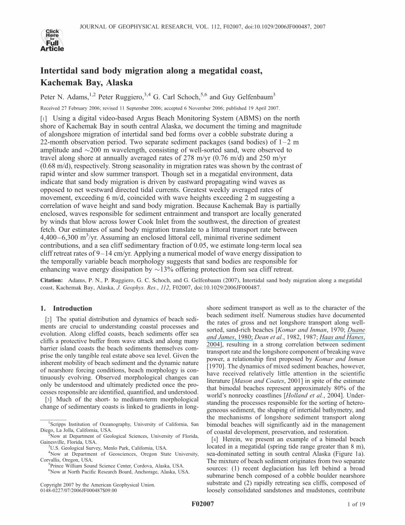
only during periods when the winds blow from the west(Figure 13), the orientation with near-maximum fetch.During a 4-day interval in late December 2003 (interval 1on Figure 13), strong winds (10–20 m/s) blew consistentlyfrom the west (260�–290�), forcing large wave heights witha daily moving average of approximately 2.5 m. Conversely,during a strong wind period in January 2004 (interval 2 onFigure 13), when 10–20 m/s winds blew from the northeast,wave heights did not respond because of the limited fetch,barely exceeding 0.5 m.

4.5. Sand Body Forcing

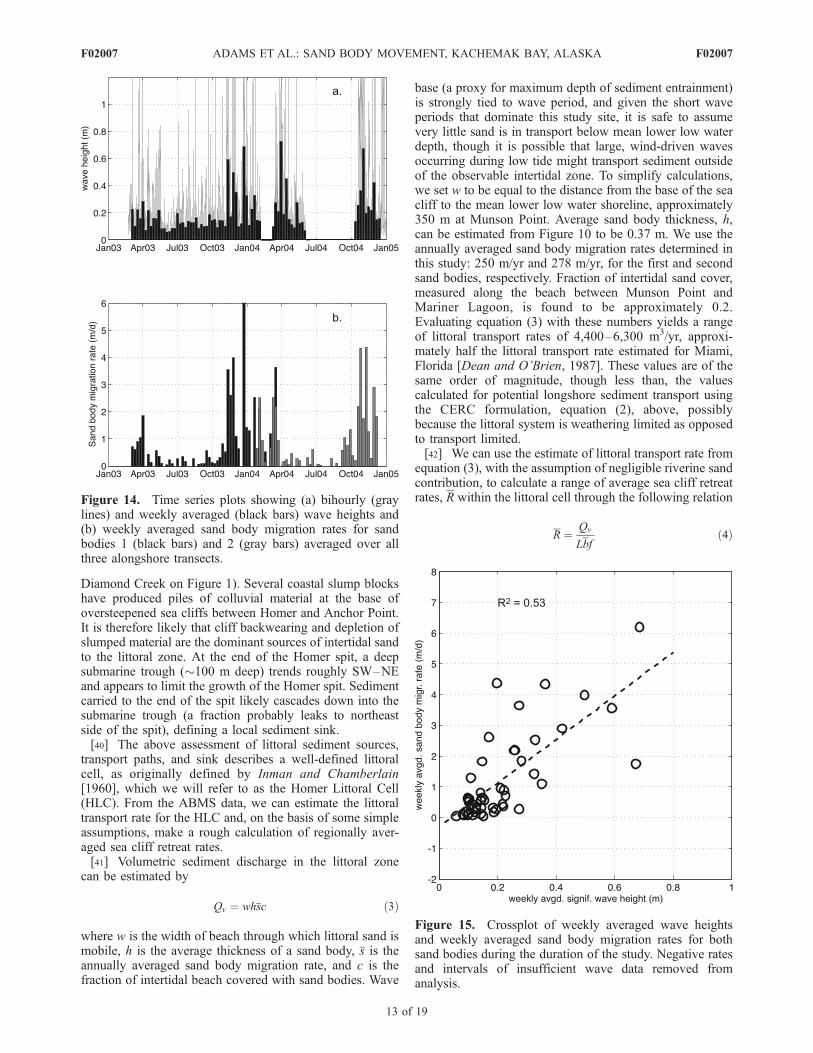
[36] To understand the relationship between the observedtemporal pattern of sand body migration and wave forcing,we plot weekly averaged sand body migration rates (aver-aged for each of the three shore parallel guide transects: AT-1,AT-2, and AT-3) against the time series of weekly averagedwave heights measured in Kachemak Bay (Figure 14).During intervals of high wave conditions in winter, sandbody migration rates are greatest, often exceeding 3 m/dduring several winter weeks of 2003 and 2004, reaching amaximum of >6 m/d in late December 2003. This forcingresponse relationship is further investigated on the corre-lation plot in Figure 15, where negative sand body migra-tion rates have been removed from the data set, as havedata collected during weeks where there were insufficientwave height measurement to accurately characterize thewave field (weeks in which fewer than 80 wave heightreadings were collected). The correlation is found to besignificant at the 95% confidence interval. Figure 15illustrates the general correlation between wave heightand sand body migration rate, but the scatter of datasuggests that there may be an uninvestigated variableinfluencing the migration rate. If the simple linear depen-dence of rate on wave height is assumed, the relationshiptakes the following form:

R ¼ 7:1H � 0:3 ð1Þ

where R is weekly averaged sand body migration rate(in meters/day) and H is weekly averaged wave height

Figure 9. Comparison of cross-shore profiles generatedwith Argus tidal-contouring method (gray data points) anddifferential GPS survey of June 2003 (black data points).Good agreement of data above elevations of 1 m (meanlower low water (MLLW)).

F02007 ADAMS ET AL.: SAND BODY MOVEMENT, KACHEMAK BAY, ALASKA

9 of 19

F02007

(in meters). The function given in equation (1) is not forcedthrough the origin of the correlation plot and the negativey-intercept value may be due to transport by currentsoriginating from other processes in a direction opposite towave-induced transport.[37] This simple relationship, equation (1), may underes-

timate the role played by incident wave direction as previous

studies have suggested a link between the longshore com-ponent of wave power and bed load sediment flux [Komarand Inman, 1970]. Because the correlation between migra-tion rate and wave height (Figure 15) is not particularlystrong, we explore the relationship between predicted long-shore sediment transport and observed sand body migration.To do so, we use the CERC equation presented in the

Figure 10. Cross-shore profiles generated by tidal-contouring method applied to Argus data for mid-March, mid-June, mid-September, and mid-December profiles along transects CT-1, CT-2, and CT-3.Note the vertical extent of the sand body visible on line CT-2.

F02007 ADAMS ET AL.: SAND BODY MOVEMENT, KACHEMAK BAY, ALASKA

10 of 19

F02007

Coastal Engineering Manual [U.S. Army Corps of Engi-neers, 2002]

QL ¼ Krf

ffiffiffig

p

16g1

�2 rs � rf� �

1� nð Þ

0B@

1CAH

5�2

b sin 2abð Þ ð2Þ

in which K is an empirical proportionality constant (set to0.6), g is the gravitational acceleration constant, g is the

breaker index (ratio of breaking wave height to breakingwave water depth, set to 0.78), rs and rf are sediment andfluid densities respectively, n is the in-place sedimentporosity (set to 0.4), Hb is the breaking wave height, and ab

is the breaking wave angle. Hb and ab are computedthrough a simple linear shoaling calculation. QL is correctedby multiplying by the fraction of beach covered by sandbodies (0.2) and the fraction of time within the tidal cyclethat sand bodies are submerged (0.44). Cumulative potentiallongshore sediment transport predicted by equation (2), and

Figure 11. High-resolution, differential GPS-derived, elevation contours of Munson Point–Homer beachdraped over ABMS-merged photos derived from June 2003 survey (a) and July 2004 survey (b). (c) Beachvolume change map. Note significant changes in beach volume associated with sand body migration.

F02007 ADAMS ET AL.: SAND BODY MOVEMENT, KACHEMAK BAY, ALASKA

11 of 19

F02007

corrected for fraction of cover and duration of submergence,for Kachemak Bay conditions starting in May 2003 isplotted with migration data for the first sand body observedin the study (Figure 16). Periods of high predicted potentialsediment transport coincide with times of rapid sand bodymigration, most notably in November and late December of2003. The total potential sediment transport calculated forthe period shown in Figure 16 (slightly less than one year) isapproximately 15,000 m3, a value that will be used forcomparison in an independent calculation of littoralsediment transport discussed below.

5. Discussion

[38] The unique combination of tidal range, gentle bathy-metric slope, bimodal size distribution of beach sediments,and strong seasonality makes the north shore of KachemakBay an ideal site to document the behavior of mobilenearshore bed forms within the intertidal zone. Data col-lected during this study affords the opportunity to speculateon (1) the local littoral sediment budget, (2) the physicalprocesses dominating littoral sediment transport in the area,and (3) the effect of migrating sand bodies on wave energyattenuation and sea cliff protection.

5.1. Littoral Sediment Budget

[39] The pattern of longshore sediment transport, asdocumented by the ABMS images in this study, is eastwardtoward the Homer spit. North of Anchor Point (Figure 1),coastal sedimentary landforms suggest northward longshoresediment transport up Cook Inlet. In agreement with thelandform evidence, the Iliamna Jet, an atmospheric phe-nomenon (low-level jet) responsible for strong winds fromthe west across Cook Inlet, has been imaged with syntheticaperture radar [Monaldo, 2000; Olsson et al., 2003]. Whenthe Iliamna Jet is active, strong winds from the mostadvantageous fetch direction (�250�) create waves whoserays approach Anchor Point, and split to drive longshorecurrents north of the point northward up Cook Inlet, andlongshore currents east of the point eastward toward Homer.This implies that the sands passing by the ABMS site atMunson Point, are derived from sources along the 30 kmstretch of coastline between Anchor Point and Homer, eitherfrom riverine inputs or bluff failures. We speculate that thereis very little riverine contribution of sediment to the littoralsystem from the small catchment area, low-discharge,coastal streams (Travers Creek, Troublesome Creek, and

Figure 12. Environmental conditions in Kachemak Bayfrom 1 January 2003 to 31 December 2005. (a) Wind speedsmeasured at Flat Island meteorological station (see Figure 1).(b) Wind direction measured at Flat Island. (c) Wave heightsmeasured by nearshore wave gage in 4 m water depthoffshore of Munson Point field site. (d) Tidal record asmeasured at Seldovia, across Kachemak Bay from Homer.Datum equals mean lower low water. Dark lines on windspeed and wave height time series are daily movingaverages.

Figure 13. Three month window of environmental con-ditions during the winter of 2003–2004 in Kachemak Bay.(a) Wind speeds measured at Flat Island meteorologicalstation (see Figure 1). (b) Wind direction measured at FlatIsland. (c) Wave heights measured by nearshore wave gagein 4 m water depth offshore of Munson Point field site (seeFigure 1). Dark lines on wind speed and wave height timeseries are daily moving averages. Note correspondence oflarge waves with strong westerly winds during interval 1and small waves in spite of strong winds during interval 2.

F02007 ADAMS ET AL.: SAND BODY MOVEMENT, KACHEMAK BAY, ALASKA

12 of 19

F02007

Diamond Creek on Figure 1). Several coastal slump blockshave produced piles of colluvial material at the base ofoversteepened sea cliffs between Homer and Anchor Point.It is therefore likely that cliff backwearing and depletion ofslumped material are the dominant sources of intertidal sandto the littoral zone. At the end of the Homer spit, a deepsubmarine trough (�100 m deep) trends roughly SW–NEand appears to limit the growth of the Homer spit. Sedimentcarried to the end of the spit likely cascades down into thesubmarine trough (a fraction probably leaks to northeastside of the spit), defining a local sediment sink.[40] The above assessment of littoral sediment sources,

transport paths, and sink describes a well-defined littoralcell, as originally defined by Inman and Chamberlain[1960], which we will refer to as the Homer Littoral Cell(HLC). From the ABMS data, we can estimate the littoraltransport rate for the HLC and, on the basis of some simpleassumptions, make a rough calculation of regionally aver-aged sea cliff retreat rates.[41] Volumetric sediment discharge in the littoral zone

can be estimated by

Qv ¼ whsc ð3Þ

where w is the width of beach through which littoral sand ismobile, h is the average thickness of a sand body, s is theannually averaged sand body migration rate, and c is thefraction of intertidal beach covered with sand bodies. Wave

base (a proxy for maximum depth of sediment entrainment)is strongly tied to wave period, and given the short waveperiods that dominate this study site, it is safe to assumevery little sand is in transport below mean lower low waterdepth, though it is possible that large, wind-driven wavesoccurring during low tide might transport sediment outsideof the observable intertidal zone. To simplify calculations,we set w to be equal to the distance from the base of the seacliff to the mean lower low water shoreline, approximately350 m at Munson Point. Average sand body thickness, h,can be estimated from Figure 10 to be 0.37 m. We use theannually averaged sand body migration rates determined inthis study: 250 m/yr and 278 m/yr, for the first and secondsand bodies, respectively. Fraction of intertidal sand cover,measured along the beach between Munson Point andMariner Lagoon, is found to be approximately 0.2.Evaluating equation (3) with these numbers yields a rangeof littoral transport rates of 4,400–6,300 m3/yr, approxi-mately half the littoral transport rate estimated for Miami,Florida [Dean and O’Brien, 1987]. These values are of thesame order of magnitude, though less than, the valuescalculated for potential longshore sediment transport usingthe CERC formulation, equation (2), above, possiblybecause the littoral system is weathering limited as opposedto transport limited.[42] We can use the estimate of littoral transport rate from

equation (3), with the assumption of negligible riverine sandcontribution, to calculate a range of average sea cliff retreatrates, R within the littoral cell through the following relation

R ¼ Qv

Lbfð4Þ

Figure 14. Time series plots showing (a) bihourly (graylines) and weekly averaged (black bars) wave heights and(b) weekly averaged sand body migration rates for sandbodies 1 (black bars) and 2 (gray bars) averaged over allthree alongshore transects.

Figure 15. Crossplot of weekly averaged wave heightsand weekly averaged sand body migration rates for bothsand bodies during the duration of the study. Negative ratesand intervals of insufficient wave data removed fromanalysis.

F02007 ADAMS ET AL.: SAND BODY MOVEMENT, KACHEMAK BAY, ALASKA

13 of 19

F02007

where L is the length of cliffed coast within the HLC, b isthe average cliff height and f is the fraction of unconsoli-dated cliff material that is immediately incorporated intolongshore littoral transport upon cliff failure. Using therange of littoral transport rates derived from equation (3),L = 30 km, b = 10 m, and an estimate of f = 0.05 (derivedfrom the observed thickness of unconsolidated sand coverdraped over the Upper Miocene to Pliocene Beluga andSterling Formations comprising the sea cliffs [Flores et al.,1997]) we obtain a range of temporally averaged sea cliffretreat rates from 9–14 cm/yr. Given the episodic nature ofsea cliff failure, however, retreat may occur as large (severalmeters) block failures every few centuries during anom-alously vigorous storm conditions. Our calculation of seacliff retreat rates is roughly an order of magnitude lower thanthose determined by Baird and Pegau [2004] (�1m/yr). Thismay reflect that our rates represent the present-day yearlyaveraged values, whereas the rapid rates determined byBaird and Pegau’s [2004] historical air photo analysisrepresent a transient response to the rapid subsidenceexperienced by the 1964 Good Friday earthquake.

5.2. Littoral Processes: Wave Dominated VersusCurrent Dominated

[43] ABMS camera monitoring of beach morphologywithin the intertidal zone reveals that sand bodies move atvariable rates, but in consistent directions. Rapid movementis well correlated to large waves, which are correlated tostrong winds blowing from the west–southwest. The tem-poral correlation of episodic sand body migration and largewave events in the bay suggests that littoral sedimenttransport is wave event driven, but other plausible sedimenttransport forcing mechanisms may be operating within thesystem and should be examined, particularly tidal currentsassociated with bay circulation, and wind-generated long-shore currents.[44] Cold, nutrient-rich water flows into Kachemak Bay

from the Gulf of Alaska along the southern shore, swirlsinto two surface gyres within the inner bay, and moves outof the bay along the north shore [Burbank, 1977]. Thiscirculation pattern, documented with drifter data by Schochand Chenelot [2004] and illustrated in Figure 3, wouldmove sediment westward along the north shore of the baytoward Cook Inlet, but the sand body migration data hereinshow only eastward movement. Furthermore, a typical sandbody occupies a vertical position on the beach profilebetween 1.75–3.25 m above mean lower low water, whichindicates complete subaerial exposure during 30% of thetime-integrated tidal elevation record and complete submer-gence during 44% of the time-integrated tidal elevationrecord (Figure 17). When the flooding or ebbing tidalcurrent velocity is at its maximum (at the inflection pointsof the tidal record curve), a typical sand body is notsubmerged, hence sediment is not accessible by the swiftesttidal currents. To examine the potential for transport by tidalcurrents when the sand body is submerged, we combine the‘‘law of the wall’’ logarithmic turbulent velocity profile

us;c

u*

¼ 1

kln

z

zo

� �ð5Þ

with the Shields criterion for sediment entrainment

qc ¼tb

rs � rf� �

gdð6Þ

Figure 16. (a) Time series of potential sediment transportat Munson Point site calculated using equation (2). (b) Timeseries of sand body position for first sand body observed instudy.

Figure 17. (a) Cross-shore profile of intertidal beach at CT-2 showing vertical extent of sand body.(b) Frequency distribution of hourly tidal elevation observations during this study. Dashed lines showelevation of mean higher high water (MHHW), mean sea level (MSL), mean lower low water (MLLW),sand body crest, and sand body base.

F02007 ADAMS ET AL.: SAND BODY MOVEMENT, KACHEMAK BAY, ALASKA

14 of 19

F02007

and the relationship between basal shear stress and shearvelocity

tb ¼ rf u2

*ð7Þ

to obtain

us;c �1

kln

z

zo

� � ffiffiffiffiffiffiffiffiffiffiffiffiffiffiffiffiffiffiffiffiffiffiffiffiffiffiffiffiffiqc rs � rf� �

gd

rf

vuut ð8Þ

us,c is the critical surface velocity required to entrainsediment of size d, within a flow depth of z, for a roughnessheight of zo, where k is von Karman’s constant (0.4 for clearwater), tb is the basal shear stress, u

*is the shear velocity,

qc is the Shields parameter, rs and rf are sediment and fluiddensities respectively, and g is the gravitational accelerationconstant. If us,c is greater than the right-hand side ofequation (8), then entrainment by a ‘‘steady’’ tidal current ispossible. An unknown quantity in equation (8) is theroughness height, zo, on the bed. A particularly ‘‘smooth’’

bed might have a roughness height controlled by the particlesize (zo = d/30), suggesting that a relatively sluggish tidalcurrent could provide sufficient basal shear stress to entrainthe sediment. However, if bed forms are present, theroughness height is substantially increased thereby slowingthe flow. The roughness height is similarly increased bywave-current interaction [Ribberink, 1998].[45] Figure 18 shows an analysis of potential entrainment

by tidal currents for typical spring tidal cycle along thenorth shore of Kachemak Bay using a value of 0.03 for theShields parameter and a sediment particle size of 0.29 mm.It is noted that this is the minimum value of the Shieldsparameter necessary for incipient grain motion, though weexpect a higher value should be used to mobilize the entirebed form. Figure 18a shows water level elevations at theMunson Point site on 14 June 2003. Figure 18b showsthe submergence depth, z in equation (8), over the crest ofthe sand body depicted in Figure 17a, during all times ofsubmergence during the chosen tidal cycle. Using ABMSimages taken with a frequency of 15 min over a complete

Figure 18. Analysis of tidal current potential for sediment entrainment. (a) Water surface elevationmeasurements during one complete spring tidal cycle from Kachemak Bay field site on 14 June 2003.(b) Submergence depth over crest of sand body shown in Figure 17a. (c) Surface velocity of tidal currentderived from ABMS shoreline position measurements throughout one tidal cycle. (d) Absolute value ofsurface velocity of tidal current (solid line) and critical entrainment surface velocity, us,c, calculated withequation (8).

F02007 ADAMS ET AL.: SAND BODY MOVEMENT, KACHEMAK BAY, ALASKA

15 of 19

F02007

tidal cycle we derive a time series of cross-shore currentvelocity estimated by temporal measurements of horizontaltidal inundation and use these data as a proxy for surfacetidal current velocity (Figure 18c), to evaluate times ofpotential entrainment by tidal currents in Figure 18d. Toobtain cross-shore tidal current velocities, shoreline posi-tions on each ABMS plan view photo were chosen alongthe same cross-shore transect. The linear difference inshoreline position divided by the difference in time stampsfor each ABMS photo (15 min) yielded the velocity.Therefore this method accounts for cross-shore variationin beach slope. The proxy tidal current velocities on thebeach are an order of magnitude slower than tidal currentvelocities in deeper water, as measured by drifter dataexperiments [Schoch and Chenelot, 2004]. Dashed lineson Figure 18d show calculations, using equation (8), of sur-face current velocities required to entrain sediment on the crest(highest elevation) of the sand body depicted in Figure 17a.The solid line shows the absolute value of the surfacevelocity of the ABMS-derived tidal current generated dur-ing the tidal cycle. Even at maximum estimated surfacevelocity, the tidal current on the beach at Munson Point doesnot generate a basal shear stress sufficient to entrain themedium-grained sand that comprises the sand bodies exam-ined in this study. This is not surprising given that the set-ting is a shallow water open beach environment where thetidal current is only a small fraction of wave generatedcurrents and swash velocities.[46] The potential for sediment transport by wind-gener-

ated currents is difficult to isolate at the Munson Point site,because the dominant wind direction coincides with thedominant wave approach direction. On the basis of the workof Whitford and Thornton [1993], we estimate that windforcing exceeds one-quarter of the wave forcing less than10% of the time during our study. Though it may be true thatmuch of the sand body migration occurs during the strongwind and wave events, longshore current augmentation bywind is unlikely to constitute the majority of longshoresediment transport forcing at the Munson Point site.[47] Because of (1) the observed direction of sand body

movement, (2) the temporal correlation of large waveevents with sand body migration rate, (3) the unfavorableconditions for sand entrainment by the tidal currents, and(4) the speculated small fraction of longshore currentaugmentation by wind, we posit that sand transport (sandbody migration) at the Munson Point site is dominated bywaves and wave-generated longshore currents.

5.3. Wave Energy Dissipation

[48] We hypothesize that the presence of intertidal sandbodies decreases the amount of wave energy delivered tosea cliffs and the upper beach face. To quantify thedissipative effects, we use a well-known model of surf zonewave energy dissipation [Thornton and Guza, 1983] tosimulate wave energy losses on the beaches at the MunsonPoint study site. A detailed numerical modeling study wasconducted for a range of wave conditions [Adams andRuggiero, 2005]. Below, we summarize the modeling workand interpret the results within the context of natural coastalbluff protection.[49] Several existing models that predict decay of wave

heights and wave energy dissipation due to frictional drag

and wave breaking within shallow water have been suc-cessfully tested against field data [e.g., Thornton and Guza,1983; Dally et al., 1985; Baldock et al., 1998; Battjes andJanssen, 1978]. The common starting point in the develop-ment of these models is the wave energy flux balance

@ ECg

� �@x

¼ �ef � eb ð9Þ

where E is wave energy density. Cg is wave group speeddefined by

Cg ¼C

21þ 2kh

sinh 2khð Þ

� �ð10Þ

ef is the loss of wave energy flux due to friction and eb is theloss of wave energy flux due to wave breaking, k is thewave number, defined as 2p/L (L is the wavelength), and his the local water depth. The majority of the energy is lost inwave breaking and the turbulence associated with thepropagation of broken surf bores.[50] We employ the model proposed by Thornton and

Guza [1983], in which the dissipation functions, for frictionand wave breaking, respectively, are defined as

ef ¼ rcf1

16ffiffiffip

p 2pf Hrms

sinh kh

� �3ð11Þ

and

eb ¼3

ffiffiffip

p

16rgB3f

H5rms

g2h31� 1

1þ Hrms=ghð Þ2� �5=2

264

375 ð12Þ

where cf is a bed friction coefficient, f is average frequencyof incident wave field, Hrms is the root-mean-square waveheight within the surf zone, B is a breaker coefficient(usually set to 1), and g is the depth-limited wave breakingcoefficient.[51] Sample model results for midtide and moderate wave

conditions (Ho = 1 m, T = 4 s) are illustrated in Figure 19and illustrate the effects of different intertidal bathymetry(presence versus absence of sand body) on the spatialpattern of wave energy dissipation through friction andbreaking. The intertidal profiles beneath the sand body areidentical for June and December of 2003 (Figure 19) as arethe input wave conditions for each of the two simulations.Therefore it can be inferred that any differences in thespatial pattern of wave energy dissipation are attributable tothe sand body. Maximum dissipation due to wave breakingis roughly 50 times greater than maximum dissipation dueto friction (Figure 19) justifying our focus, hereafter, solelyupon dissipation associated with wave breaking processes.Dissipation by wave breaking corresponds to steepness ofbathymetric profile; the sand body appears to offer a naturalprotection to the upper beach face and sea cliffs through twomechanisms: (1) by moving the locus of wave breakingseaward and (2) by increasing energy expenditure associatedwith the turbulence of wave breaking.[52] To assess the dissipative effects of the sand wave

over a range of tidal heights and wave conditions, we

F02007 ADAMS ET AL.: SAND BODY MOVEMENT, KACHEMAK BAY, ALASKA

16 of 19

F02007

evaluate the wave energy flux at cross-shore locationsmarking the seaward and landward extents of the sandbody, respectively (PS and PL, on Figure 19), approximately115 m apart. The difference in wave energy flux betweenthese two locations is equal to the quantity of wave energylost over the intervening cross-shore reach.[53] Figure 20 shows the results of 34 simulations of

cross-shore wave energy dissipation over both the June andDecember profiles at varying tide levels (2 m to 6 m abovemean lower low water) for extreme wave conditions inKachemak Bay (Ho = 2 m, T = 8 s). Figures 20a and 20bshow that wave height and wave energy flux, respectively,decrease shoreward and respond to the presence of theintertidal sand body. Figures 20c and 20d display thepercent wave height decrease and percent wave energy fluxloss between positions PS and PL, respectively. In thepresence of the sand body, wave heights and energy fluxesare lowered to greater proportions than in the absence of thesand body, irrespective of tide. The amount by which wavedissipation is enhanced (taken as the difference between theblack and gray curves on Figures 20c and 20d) is plotted inFigures 20e and 20f. Maximum dissipation enhancementsare 19% and 13% for wave height and wave energy flux,respectively, and occur at midtide to high tide for extremeKachemak Bay wave conditions.[54] As noted in previous work [Adams and Ruggiero,

2005] there is a positive feedback operating within the

intertidal zone; the existence of a sand body enhances waveenergy dissipation over the sand body, which in turnincreases the amount of turbulent energy used to entrainand mobilize the sediments, propagating the sand bodyalong shore, provided that there is an oblique componentto the incident wave field. As viewed from the perspectiveof the sea cliff, there is a potentially valuable negativefeedback; large waves attack the sea cliff, driving retreat,however the eroded material now in front of the sea clifflowers the assailing energy of future incoming waves,protecting the cliff from further retreat. Shutting off thissediment supply, by anthropogenically armoring the coast-line, could eventually remove the dissipative effect providedby the sediment and may foster more dramatic cliff erosionevents during anomalously large wave conditions.[55] Lastly, we note the interesting flow and sediment

transport mechanics that arise in a mixed sediment envi-ronment subject to the combined influence of waves andtides. The focus of our study has been to document themovement of discrete sand packages over a gravel/cobblesubstrate, and the consequences of the sand body migration.

Figure 19. (a) Bathymetric input conditions and (b) sampleoutput from numerical model of wave energy dissipationapplied to Munson Point study site for moderate waveconditions (Ho = 1 m, T = 4 s). Gray and black lines representJune 2003 and December 2003 results, respectively.

Figure 20. Wave energy dissipation modeling results forextreme Kachemak Bay wave conditions (Ho = 2 m, T = 8 s).(a) Wave heights through the surf zone for all 34 simulations.Gray lines computed for June profile (sand body present).Black lines computed for December profile (sand bodyabsent). (b) Simulated wave energy fluxes. (c) Percentagewave height loss between PS and PL. (d) Percentage waveenergy flux losses. (e) Dissipation enhancement for sandwave presence derived from wave height output (differenceof gray and black curves in Figure 20c). (f) Dissipationenhancement for sand wave presence derived from waveenergy flux output (difference of gray and black curves inFigure 20d).

F02007 ADAMS ET AL.: SAND BODY MOVEMENT, KACHEMAK BAY, ALASKA

17 of 19

F02007

We have not investigated in detail the self-organization of thesand bodies themselves, or the mechanics of sand bodymovement over gravel, but hypothesize that the two processesare coupled. Increased turbulence over the hydrodynamicallyrougher cobble substrate could lead to preferential advectionof sand grains toward areas of higher sediment concentration,e.g., sand bodies, and away from the interstitial spacesbetween individual cobbles. The discrete sand bodies result-ing from this hypothesized self-organization mechanism thenfeedback with the nearshore hydrodynamics by increasingwave breaking and wave-induced currents which in turnmobilize the sand bodies over the cobble substrate. Futurework will attempt to characterize and quantify, over varioustimescales, the coupled sediment transport dynamics andmorphological development of this prototypical mixed sed-iment system.

6. Conclusions

[56] This study documents a quantitative link betweenoceanic forcing and nearshore morphologic change. On thebasis of a 22 monthlong set of digital video imagery thatshow the migration of sand bodies over a cobble substrateand data documenting local environmental conditions, weconclude that seasonally variable migration of 20–200 mlong, �1 m thick, self-organized, intertidal sand bodies isdriven by episodes of high wave activity, and not driven bytidal or baroclinic circulation currents within KachemakBay. During the winter, these sand bodies move at weeklyaveraged rates of >2 m/d, and during large storms wedocument migration as fast as 6 m/d. Sufficient waves areonly generated within lower Cook Inlet, adjacent to Kache-mak Bay, during periods of strong sustained southwesterlywinds, a condition that occurs as a direct result of theIliamna Jet meteorological phenomenon. These measure-ments of sand body migration provide estimates of littoralsediment transport rates and sea cliff retreat rates within theHomer Littoral Cell. It is further quantified that sand bodiesprovide a natural buffer to sea cliff retreat through waveenergy dissipation.

[57] Acknowledgments. This research was made possible by fundingfrom the U.S. Geological Survey and a NOAA National Estuarine ResearchReserve Graduate Fellowship to P.N.A. Logistical support was provided bythe Kachemak Bay Research Reserve. Support for G.C.S. was provided bygrants from the Cook Inlet Regional Citizens Advisory Council and theCoastal Impact Assessment Program. Lagrangian drifter trajectories wereprovided by Mark Johnson through Minerals Management Service grant882 for the Coastal Marine Institute study of Cook Inlet water and icedynamics. Special thanks go to Paul Eneboe, Carey Meyer, the City ofHomer, Scott Pegau, Steve Baird, Jodi Harney, Jodi Eshleman, RyanCoppersmith, Joan Oltman-Shay, Michael Horgan, Chad Budworth, andNorthwest Research Associates. This manuscript benefited greatly fromcomments by Jon Warrick, Dave Rubin, Doug Inman, Bob Anderson,Patricia Wiberg, and two anonymous reviewers.

ReferencesAarninkhof, S. (2003), Nearshore Bathymetry Derived From Video Ima-gery, Delft Univ. Press, Netherlands.

Adams, P. N., and P. Ruggiero (2005), Wave energy dissipation by intertidalsand waves on a mixed-sediment beach, paper presented at Coastal Dy-namics ’05, Am. Soc. of Civ. Eng., Barcelona, Spain.

Anthony, E. J., F. Levoy, and O. Monfort (2004), Morphodynamics ofintertidal bars on a megatidal beach, Merlimont, northern France, Mar.Geol., 208, 73–100.

Ashley, G. M. (1990), Classification of large-scale subaqueous bed forms:A new look at an old problem, J. Sediment. Petrol., 60, 160–172.

Baird, S., and W. S. Pegau (2004), City of Homer coastal characterizationand change analysis, report, Coastal Impact Assistance Program, Homer,Alaska.

Baldock, T. E., P. Holmes, S. Bunker, and P. V. Weert (1998), Cross-shorehydrodynamics within an unsaturated surf zone, Coastal Eng., 34, 173–196.

Battjes, J. A., and J. P. F. M. Janssen (1978), Energy loss and set-up due tobreaking of random waves, in Proceedings of the 16th InternationalConference on Coastal Engineering, pp. 569–587, Am. Soc. of Civ.Eng., Hamburg, Germany.

Bradley, D. C., T. M. Kusky, S. M. Karl, and P. J. Haeussler (1997), FieldGuide to the Mesozoic Accretionary Complex Along Turnagain Arm andKachemak Bay, South-Central Alaska: Guide to the Geology of the KenaiPeninsula, Alaska, Alaska Geol. Soc., Anchorage, Alaska.

Burbank, D. C. (1977), Circulation Studies in Kachemak Bay and LowerCook Inlet, edited by L. L. Trasky, L. B. Flagg, andD. C. Burbank, 207 pp.,Alaska Dept. of Fish and Game, Anchorage.

CERC (1984), Shore Protection Manual, U. S. Army Corps of Eng., Vicksburg,Mississippi.

Dally, W. R., R. G. Dean, and R. A. Dalrymple (1985), Wave heightvariation across beaches of arbitrary profile, J. Geophys. Res., 90,11,917–11,927.

Dean, R. G., and M. P. O’Brien (1987), Florida’s east coast inlets, shorelineeffects, and recommendations for action, report, 65 pp., Coastal andOcean Eng. Dept. Univ. of Fla., Gainesville.

Dean, R. G., E. P. Berek, C. G. Gable, and R. J. Seymour (1982), Long-shore transport determined by an efficient trap, paper presented at the18th Coastal Engineering Conference, Am. Soc. of Civ. Eng., CapeTown, South Africa.

Dean, R. G., E. P. Berek, K. R. Bodge, and C. G. Gable (1987), NSTSmeasurements of total longshore transport, paper presented at CoastalSediments ’87, Am. Soc. of Civ. Eng., Gainesville, Fla.

Duane, D. B., and W. R. James (1980), Littoral transport in the surf zoneelucidated by an Eulerian sediment tracer experiment, J. Sediment. Pet-rol., 50, 929–942.

Eckel, E. B. (1970), The Alaska earthquake, March 27, 1964: Lessons andconclusions, U.S. Geol. Surv. Prof. Pap., 546, 57 pp.

Flores, R. M., et al. (1997), Stratigraphic Architecture of the Tertiary Allu-vial Beluga and Sterling Formations, Kenai Peninsula, Alaska: Guide tothe Geology of the Kenai Peninsula, Alaska, Alaska Geol. Soc., Anchorage,Alaska.

Haas, K. A., and D. M. Hanes (2004), Process based modeling of totallongshore sediment transport, J. Coastal Res., 20, 853–861.

Holland, K. T., R. A. Holman, T. C. Lippmann, J. Stanley, and N. Plant(1997), Practical use of video imagery in nearshore oceanographic fieldstudies, J. Oceanic Eng., 22, 81–92.

Holland, K. T., J. M. Kaihatu, and T. R. Keen (2004), The influence ofsediment heterogeneity on coastal hydrodynamics, Eos Trans. AGU,84(52), Ocean Sci. Meet. Suppl., Abstract OS41L-03.

Holman, R. A., T. C. Lippmann, P. V. Oneill, and K. Hathaway (1991),Video estimation of subaerial beach profiles, Mar. Geol., 97, 225–231.

Holman, R. A., A. H. J. Sallenger, T. C. Lippman, and J. W. Haines (1993),The application of video image processing to the study of nearshoreprocesses, Oceanography, 6, 78–85.

Inman, D. L., and T. K. Chamberlain (1960), Littoral sand budget along thesouthern California coast, paper presented at the 21st International Geo-logical Congress, Int. Union of Geol. Sci., Copenhagen.

Karlstrom, T. N. V. (1964), Quaternary geology of the Kenai Lowland andglacial history of the Cook Inlet region, Alaska, U.S. Geol. Surv. Prof.Pap., 443, 69 pp.

Komar, P. D., and D. L. Inman (1970), Longshore sand transport on bea-ches, J. Geophys. Res., 75, 5527–5914.

Lippmann, T. C., and R. A. Holman (1989), Quantification of sand-barmorphology—A video technique based on wave dissipation, J. Geophys.Res., 94, 995–1011.

Lippmann, T. C., and R. A. Holman (1990), The spatial and temporalvariability of sand-bar morphology, J. Geophys. Res., 95, 11,575–11,590.

Mason, T., and T. T. Coates (2001), Sediment transport processes on mixedbeaches: A review for shoreline management, J. Coastal Res., 17, 645–657.

Monaldo, F. (2000), The Alaska SAR demonstration and near-real-timesynthetic aperture radar winds, Johns Hopkins APL Tech. Dig., 21,75–79.

Muench, R. D., H. O. Mofjeld, and R. L. Charnell (1978), Oceanographicconditions in Lower Cook Inlet: Spring and summer 1973, J. Geophys.Res., 83, 5090–5098.

Okkonen, S. (2005), Observations of hydrography and currents in centralCook Inlet, Alaska during diurnal and semidiurnal tidal cycles, OCS Stud.MMS 2004-058, Inst. of Mar. Sci. Univ. of Alaska, Fairbanks.

F02007 ADAMS ET AL.: SAND BODY MOVEMENT, KACHEMAK BAY, ALASKA

18 of 19

F02007

Olsson, P. Q., H. Yi, and K. P. Volz (2003), Numerical simulations ofcoastal wind events in the north Gulf of Alaska, paper presented at the10th Conference on Mesoscale Processes, Am. Meteorol. Soc., Portland,Oreg.

Plant, N. G., and R. A. Holman (1997), Intertidal beach profile estimationusing video images, Mar. Geol., 140, 1–24.

Reger, R. D., and D. S. Pinney (1997), Last Major Glaciation of KenaiLowland: Guide to the Geology of the Kenai Peninsula, Alaska, AlaskaGeol. Soc., Anchorage, Alaska.

Ribberink, J. S. (1998), Bed-load transport for steady flows and unsteadyoscillatory flows, Coastal Eng., 34, 59–82.

Rubin, D. M. (2004), A simple autocorrelation algorithm for measuringsediment grain size in digital images, J. Sediment. Res., 74, 160–165.

Schoch, G. C., and H. Chenelot (2004), The role of estuarine hydrody-namics in the distribution of kelp forests in Kachemak Bay, Alaska,J. Coastal Res., 45, 179–194.

Thornton, E. B., and R. T. Guza (1983), Transformation of wave heightdistribution, J. Geophys. Res., 88, 5925–5938.

U.S. Army Corps of Engineers (2002), Coastal Engineering Manual, Eng.Manual 1110-2-1100, Washington, D. C.

Whitford, D. J., and E. B. Thornton (1993), Comparison of wind and waveforcing of longshore currents, Cont. Shelf Res., 13, 1205–1218.

Whitney, J. (1994), Past experience with spill response in Cook Inlet, report,ISCOI, NOAA, Hazard. Mater. Response and Assess. Div., Anchorage,Alaska.

�����������������������P. N. Adams, Department of Geological Sciences, 241 Williamson Hall,

P.O. Box 112120, University of Florida, Gainesville, FL 32611, USA.(adamsp@ufl.edu)G. Gelfenbaum, Coastal and Marine Geology, U.S. Geological Survey,

Menlo Park, CA 94025, USA. (ggelfenbaum@usgs.gov)P. Ruggiero, Department of Geosciences, Oregon State University,

104 Wilkinson Hall, Corvallis, OR 97331-5506, USA. (ruggierp@science.oregonstate.edu)G. C. Schoch, North Pacific Research Board, 1007 W. 3rd Avenue, Suite

100, Anchorage, AK 99501, USA. (cschoch@nprb.org)

F02007 ADAMS ET AL.: SAND BODY MOVEMENT, KACHEMAK BAY, ALASKA

19 of 19

F02007