Microphone Array System for Speech Enhancement in ... - DIVA
52
Microphone Array System for Speech Enhancement in a Motorcycle Helmet Per Cornelius Nedelko Grbic Ingvar Claesson Department of Signal Processing School of Engineering Blekinge Institute of Technology Blekinge Institute of Technology Research Report 2005:05
-
Upload
khangminh22 -
Category
Documents
-
view
0 -
download
0
Transcript of Microphone Array System for Speech Enhancement in ... - DIVA
Microphone Array System forSpeech Enhancement in a
Motorcycle Helmet
Per CorneliusNedelko Grbic
Ingvar Claesson
Department of Signal ProcessingSchool of Engineering
Blekinge Institute of Technology
Blekinge Institute of TechnologyResearch Report 2005:05
Microphone array system for speechenhancement in a motorcycle helmet
P. Cornelius, N. Grbic and I. Claesson
May, 2005
Research ReportDepartment of Signal Processing
Blekinge Institute of Technology, Sweden

Abstract
In this report a real case study of the sound environment within a helmet whiledriving motorcycle is investigated. A solution to perform speech enhancement isproposed for the purpose of mobile speech communication. A microphone array,mounted onto the face shield in front of the user’s mouth, is used to capture thespatio-temporal properties of the acoustic wave field inside the helmet. The powerof the spatially spread noise within the helmet is small when standing still whileit may heavily exceed the power of the speech when driving at high speeds. Thiswill result in dramatically reduced speech intelligibility in the communicationchannel. The highly dynamic noise level imposes a challenge for existing speechenhancement solutions.
We propose a subband adaptive system for speech enhancement which consistsof a soft constrained beamformer in cascade with a signal-to-noise ratio dependentsingle microphone solution. The beamformer make use of a calibration signalgathered in the actual environment from the speaker’s position. This calibrationprocedure efficiently captures the acoustical properties in the environment.
Evaluation of the beamformer and the single microphone algorithm, both aseither parts by them selves and as a cascaded structure, together with the optimalsubband Wiener solution is presented. It is shown that a cascaded combination ofthe calibrated subband beamforming technique together with the single channelsolution outperforms either one by it self, and provides near optimal results atall noise levels.

2
Contents
1 Introduction 5
2 Problem formulation 92.1 Signal model . . . . . . . . . . . . . . . . . . . . . . . . . . . . . . 92.2 Spatio-temporal correlation . . . . . . . . . . . . . . . . . . . . . 102.3 The Wiener solution . . . . . . . . . . . . . . . . . . . . . . . . . 11
3 Data evaluation 133.1 Data acquisition . . . . . . . . . . . . . . . . . . . . . . . . . . . . 133.2 Noise and speech analysis . . . . . . . . . . . . . . . . . . . . . . 14
3.2.1 Spectrum analysis . . . . . . . . . . . . . . . . . . . . . . . 143.2.2 SNR analysis . . . . . . . . . . . . . . . . . . . . . . . . . 153.2.3 Coherence and eigenvalue analysis . . . . . . . . . . . . . . 18
4 Implementation 234.1 The speech enhancement beamformer . . . . . . . . . . . . . . . . 23
4.1.1 Filterbank . . . . . . . . . . . . . . . . . . . . . . . . . . . 234.1.2 Spatially Constraind Calibrated weight RLS (SCCWRLS) 244.1.3 Adaptive gain equalizer . . . . . . . . . . . . . . . . . . . . 25
5 Evaluations 275.1 Parameters settings . . . . . . . . . . . . . . . . . . . . . . . . . . 275.2 Output SNR . . . . . . . . . . . . . . . . . . . . . . . . . . . . . . 275.3 Noise suppression and Speech distortion . . . . . . . . . . . . . . 29
5.3.1 Performance measures . . . . . . . . . . . . . . . . . . . . 295.3.2 Noise suppression . . . . . . . . . . . . . . . . . . . . . . . 305.3.3 Speech distortion . . . . . . . . . . . . . . . . . . . . . . . 32
6 Summary and conclusions 37
A Spectrograms 39
3

4
Chapter 1
Introduction
The use of helmets are essential and unavoidable in many situations. They maybe used to reduce the risk of head injuries as well as providing comfort in rowdyand noisy environments. In order to circumvent the restrictions of speech commu-nication imposed by wearing a helmet a reliable duplex communication channelneeds to be installed into the helmet. The feature of communication can be usedfor both distant human-to-human speech communication as well as human-to-machine communication where additional speech recognition devices may be usedto interpret voice commands. By using human voice commands to execute simplecontrol task or to retrieve environmental information, higher flexibility and safetycan be archived. However, surrounding noise severely degrades the performanceof such communication systems. For instance, within a helmet while drivinga motorcycle the noise is changing rapidly from almost a negligible level whenstanding still to become very high at high speeds, where the power of noise evenexceeds the power of speech. In order to provide a convenient communicationfeature in such environment, there is a need for successful speech enhancement.In this chapter, the sound environment within a helmet in a motorcycle scenariois analyzed and investigated for different driving conditions. Appropriate speechenhancement/noise reduction algorithms are proposed and evaluated.
With only one microphone available, the speech quality improvements havetraditionally been focused on the temporal/ spectral information. A commonlyused method, spectral subtraction, is a frequency domain approach which es-timates the background noise when the speaker is silent [1, 2]. The estimatedspectrum is subtracted from the noisy speech spectrum. The quality of the noiseestimate is crucial for the final result and a Voice Activity Detector (VAD) isneeded to detect speech pauses. This approach works well when the noise signalis reasonable stationary. Recently, the speech booster, a time-domain adaptivegain equalizer, was presented [3]. The input signal is divided into a number ofsubbands that are individually weighted according to the short time Signal-to-
5
6 Chapter 1. Introduction
Noise Ratio estimate (SNR) in each subband at every time instant. The methodis focusing on speech enhancement and offers low complexity, low delay and lowdistortion and operates without a VAD. As for most single channel methods, theperformance is heavily dependant on good SNR.
To overcome the limitations of single-microphone temporal processing meth-ods, spatial information can be exploited by using multiple microphones [4]. Theinterest of using microphone arrays for broadband speech and audio processinghave increased in recent years. There have been a lot of interesting researchpublished in applications using different beamforming techniques, for examplehands-free voice communication in cars, hearing-aids, teleconferencing and mul-timedia applications [4, 5, 6]. With multiple microphones, the spatial informationcan be used to form beams that may be fixed or they can adaptively change ac-cording to the environment. The General sidelobe canceller (GSC) [7] presents astructure that can be used to implement a variety of adaptive beamformers. Itconsist of a fix beamformer directed towards a desired location and an adaptivefilter matrix blocking the desired source signal. However, the desired signal maybe distorted or even cancelled due to super-resolution problems [5]. By turningof the adaptation process during activity from the source signal, determined bya VAD, this problem may be solved. GSC has shown to be sensitive to reverber-ation [8]. Many other suggested beamformers such as the subspace techniquesand optimal filtering concepts rely on voice activity detection, [9, 10].
The proposed solution for noise reduction and speech enhancement is a mi-crophone array positioned within the helmet. The array is controlled by a beam-former combined with a single channel algorithm, the speech booster. The posi-tion of a speaker is assumed to be fixed inside the helmet while the noise sourceare assumed to be nonstationary in both space and time. The environment withthe microphone placement and the speaker position is difficult to describe by apriori model, whereby sequences of calibration signals can be used effectively forthe design of the beamformer. The use of calibration signals from the actualacoustical environment may provide information about source position, reverber-ation and possible microphone displacements. A constrained subband adaptivebeamformer, proposed in [11], make use of these calibration signals gathered fromthe desired position. These signals contains all necessary statistical informationabout the source and the environment. By adding a spatial constraint based onthese signals, the source signal remain almost unaltered through the beamformer,while the background noise is suppressed, [12]. The adaptation process do notneed knowledge of speech activity.
In this chapter a speech signal together with the noise field correspondingto motorcycle speeds at 50, 70, 90, 110, 130 and 150 km/h is investigated. Anefficient polyphase structure filterbank implementation of a uniform DFT filter-
Chapter 1. Introduction 7
bank is used to transform the input signal into narrow-band sub-band signals.The design method, according to [13], reduces the in-band and reconstructionaliasing effects. Results from the proposed beamformer, the speech booster andboth algorithms combined in cascade, are presented for each motorcycle speed.The beamformer works most efficiently on suppressing the noise when the signal-to-noise ratio (SNR) decreases and consequently is works better at high speeds.The single microphone algorithm performance depends heavily upon good SNRand it therefor performs best at low speeds. When both method are placed incascade the resulting solution provides significant total SNR improvement at allmotorcycle speeds. While the noise suppression increases with the combinationof these two methods, the resulting sound quality is still maintained.
8 Chapter 1. Introduction
Chapter 2
Problem formulation
2.1 Signal model
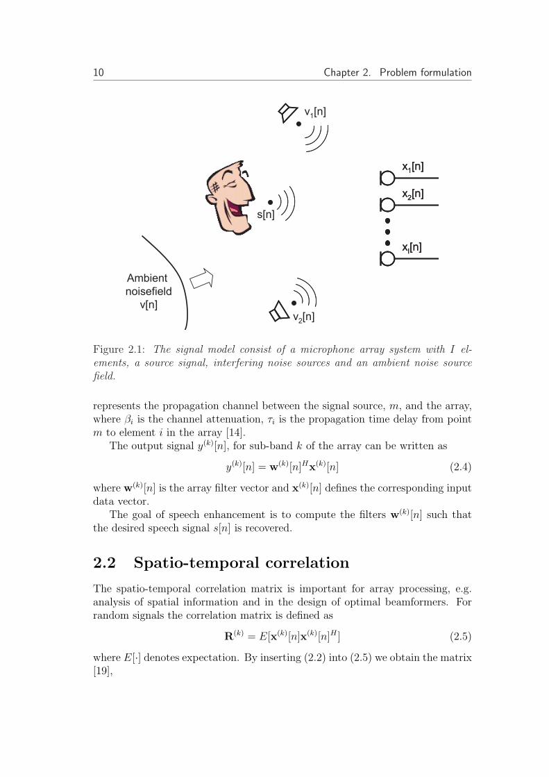
We consider a signal model where the source of interest, the speaker, is situated ina fixed position relative to the sensor array. The noise environment consists of acombination of directional noise sources, which will have changing positions, anda ambient noise field, see figure 2.1. The microphone array receive a componentfrom the speaker, s[n], and a sum of noise sources, vd[n], d = 1, . . . , D togetherwith the ambient noise field, v[n], as
xi[n] = si[n] +D∑
d=1
vdi[n] + vi[n] (2.1)
where si[n], vdi, d = 1, . . . , D and vi[n] are the i:th microphone observations ofthe signals, respectively.
The wide-band array processing is based on sub-band decomposition of theinput signals. Each sensor signal is decomposed by a filterbank, into K-complexvalued sub-band components. Each sub-band filter contains narrow-band, timedomain signals with essentially components at the central frequency fk (k =1, 2, . . . , K). Due to the sub-band decomposition we may use the well knownnarrow-band discrete-time array formulation. For a sub-band k with a certainfrequency fk, the array data vector received from M point sources, impinging ona I-element array in space, at time n, may be described by
x(k)[n] =M∑
m=1
u(k)m (t)a(f)
m + v[n] (2.2)
where v[n] is a received uncorrelated noise field vector, um[n] is the signal fromthe m point source and the array response vector (steering vector)
a(f)m (τ) = [β1e
i2πfτ1 β2ei2πfτ2 . . . βIe
i2πfτI ]T (2.3)
9
10 Chapter 2. Problem formulation
s[n]
x1[n]
x2[n]
xI[n]
x1[n]
x2[n]
xI[n]
v2[n]
Ambient
noisefield
v[n]
v1[n]
Figure 2.1: The signal model consist of a microphone array system with I el-ements, a source signal, interfering noise sources and an ambient noise sourcefield.
represents the propagation channel between the signal source, m, and the array,where βi is the channel attenuation, τi is the propagation time delay from pointm to element i in the array [14].
The output signal y(k)[n], for sub-band k of the array can be written as
y(k)[n] = w(k)[n]Hx(k)[n] (2.4)
where w(k)[n] is the array filter vector and x(k)[n] defines the corresponding inputdata vector.
The goal of speech enhancement is to compute the filters w(k)[n] such thatthe desired speech signal s[n] is recovered.
2.2 Spatio-temporal correlation
The spatio-temporal correlation matrix is important for array processing, e.g.analysis of spatial information and in the design of optimal beamformers. Forrandom signals the correlation matrix is defined as
R(k) = E[x(k)[n]x(k)[n]H ] (2.5)
where E[·] denotes expectation. By inserting (2.2) into (2.5) we obtain the matrix[19],
Chapter 2. Problem formulation 11
R = E
[M∑
m=1
|um[n]|2amaHm +
∑
l 6=m
ul[n]um[n]∗alaHm + σ2
vI
](2.6)
where σ2v is the variance of the noise field and where the sub-band index, k,
is omitted for simplicity. If the point sources are temporally uncorrelated, thematrix is reduced to
R = E
[M∑
m=1
|um[n]|2amaHm + σ2
vI
]. (2.7)
If the number of point sources M are smaller than the number of array elementsI and the response vectors are linearly independent, then the correlation matrixof eq (2.7) contains M eigenvalues. The eigenvalues are given by
λ1, λ2, . . . , λM = σ21, σ
22, . . . , σ
2M (2.8)
where σ2m is defined as
σ2m = |um[n]|2aH
mam (2.9)
The eigenvalues of any two signals, which increasingly becomes spatially (or tem-porally) coherent, tends towards providing a single eigenvalue. When the twosources have an unitary coherence, i.e. total spatial (or temporal) correlation,they add a single rank contribution to the correlation matrix of Eq. (2.6).
2.3 The Wiener solution
The optimal filter weight vector based on the Wiener solution for subband k isgiven by
w(k)opt =
[R(k)
]−1r(k)
s (2.10)
where the array weight vector, w(k)opt is arranged as
w(k)opt = [w
(k)1 , w
(k)2 , . . . , w
(k)I ] (2.11)
and where r(k)s is the cross-correlation vector defined as
r(k)s = E[x(k)[n]s(k)[n]] (2.12)
where s(k)[n] is the k:th sub-band signal corresponding to the source. It shouldbe noted that this signal is generally not accessible, while a modified Wienersolution (derived in section 4) is used instead. The output of the beamformer isgiven by
y(k) = w(k)H
opt x(k)[n]. (2.13)
These output sub-band signals are used to create a full-band output.
12 Chapter 2. Problem formulation
Chapter 3
Data evaluation
3.1 Data acquisition
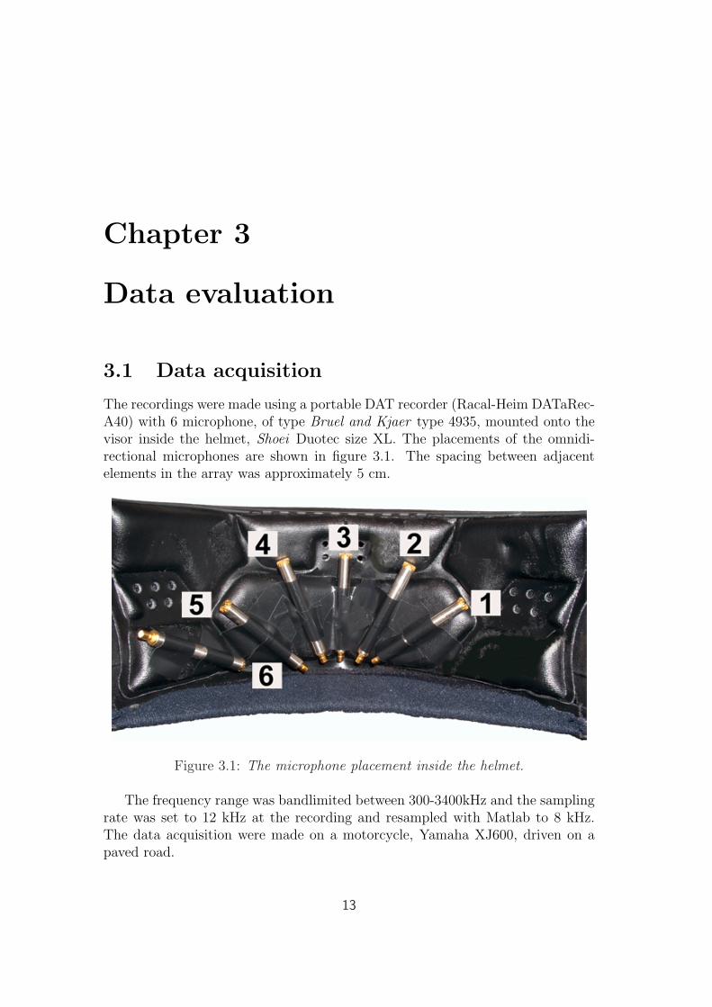
The recordings were made using a portable DAT recorder (Racal-Heim DATaRec-A40) with 6 microphone, of type Bruel and Kjaer type 4935, mounted onto thevisor inside the helmet, Shoei Duotec size XL. The placements of the omnidi-rectional microphones are shown in figure 3.1. The spacing between adjacentelements in the array was approximately 5 cm.
Figure 3.1: The microphone placement inside the helmet.
The frequency range was bandlimited between 300-3400kHz and the samplingrate was set to 12 kHz at the recording and resampled with Matlab to 8 kHz.The data acquisition were made on a motorcycle, Yamaha XJ600, driven on apaved road.
13
14 Chapter 3. Data evaluation
An utterance of the driver speaking was gartered in a quiet environment, with theengine turned off, helmet placed on the head, visor down and windshield open.This utterance was recorded at the array and the corresponding signals serve asthe desired sound source calibration signals in all of the following calculations.
Another speech signal is collected with the same conditions as above butwith the windshield closed. This signal will serve as an estimate of the speechwhile driving because a clean speech signal is not available during driving. Thecollected speech sequence is used for evaluation.
The recording was limited to six different speeds, 50, 70, 90, 110, 130 and 150km/h. While driving the motorcycle, the windshield was closed. For each fixedspeed the driver reads a number of prespecified sentences for approximately 25seconds. In order to make an analysis of the present noise at each velocity, aduration of 20 second is recorded when the driver is silence.
3.2 Noise and speech analysis
The helmet noise consist of a number of unwanted sound sources, mostly withbroad spectral content, e.g. wind, engine and tire noise. At high speeds the windnoise becomes dominant.
3.2.1 Spectrum analysis
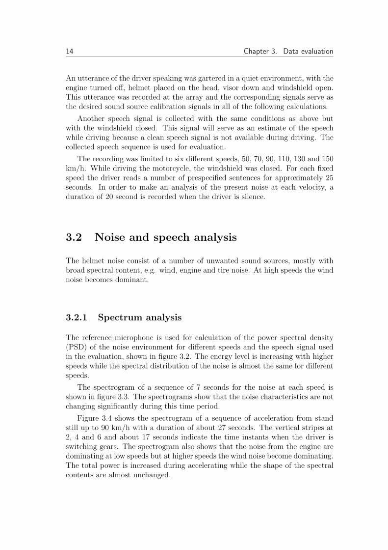
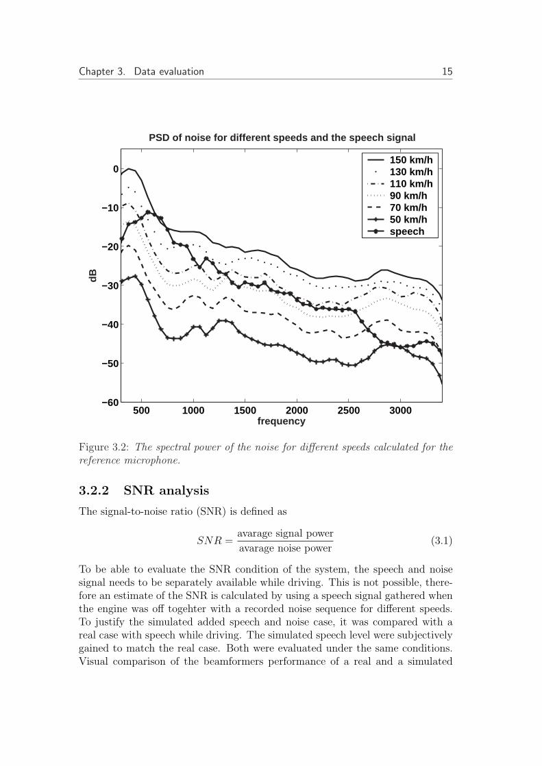
The reference microphone is used for calculation of the power spectral density(PSD) of the noise environment for different speeds and the speech signal usedin the evaluation, shown in figure 3.2. The energy level is increasing with higherspeeds while the spectral distribution of the noise is almost the same for differentspeeds.
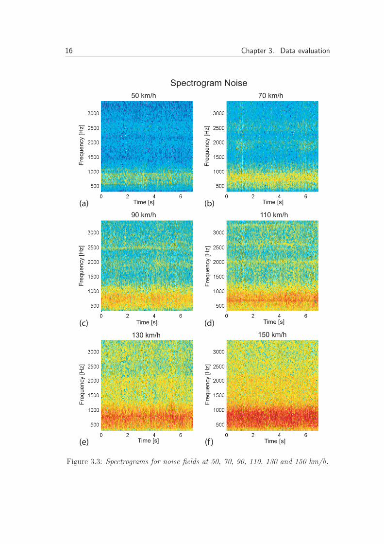
The spectrogram of a sequence of 7 seconds for the noise at each speed isshown in figure 3.3. The spectrograms show that the noise characteristics are notchanging significantly during this time period.
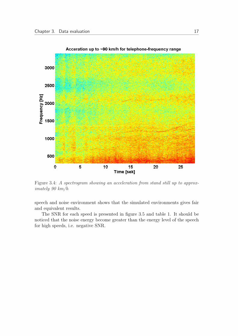
Figure 3.4 shows the spectrogram of a sequence of acceleration from standstill up to 90 km/h with a duration of about 27 seconds. The vertical stripes at2, 4 and 6 and about 17 seconds indicate the time instants when the driver isswitching gears. The spectrogram also shows that the noise from the engine aredominating at low speeds but at higher speeds the wind noise become dominating.The total power is increased during accelerating while the shape of the spectralcontents are almost unchanged.
Chapter 3. Data evaluation 15
500 1000 1500 2000 2500 3000−60
−50
−40
−30
−20
−10
0
frequency
dB
PSD of noise for different speeds and the speech signal
150 km/h130 km/h110 km/h90 km/h70 km/h50 km/hspeech
Figure 3.2: The spectral power of the noise for different speeds calculated for thereference microphone.
3.2.2 SNR analysis
The signal-to-noise ratio (SNR) is defined as
SNR =avarage signal power
avarage noise power(3.1)
To be able to evaluate the SNR condition of the system, the speech and noisesignal needs to be separately available while driving. This is not possible, there-fore an estimate of the SNR is calculated by using a speech signal gathered whenthe engine was off togehter with a recorded noise sequence for different speeds.To justify the simulated added speech and noise case, it was compared with areal case with speech while driving. The simulated speech level were subjectivelygained to match the real case. Both were evaluated under the same conditions.Visual comparison of the beamformers performance of a real and a simulated
16 Chapter 3. Data evaluation
50 km/h 70 km/h
90 km/h 110 km/h
130 km/h 150 km/h
Time [s] Time [s]
Time [s] Time [s]
Time [s] Time [s]
Fre
quency [H
z]
Fre
quency [H
z]
Fre
quency [H
z]
Fre
quency [H
z]
Fre
quency [H
z]
Fre
quency [H
z]
Spectrogram Noise
(d)
(b)
(f )(e)
(c)
(a)
Figure 3.3: Spectrograms for noise fields at 50, 70, 90, 110, 130 and 150 km/h.
Chapter 3. Data evaluation 17
Figure 3.4: A spectrogram showing an acceleration from stand still up to approx-imately 90 km/h
speech and noise environment shows that the simulated environments gives fairand equivalent results.
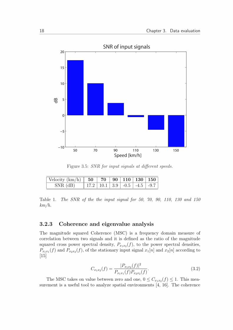
The SNR for each speed is presented in figure 3.5 and table 1. It should benoticed that the noise energy become greater than the energy level of the speechfor high speeds, i.e. negative SNR.
18 Chapter 3. Data evaluation
50 70 90 110 130 150−10
−5
0
5
10
15
20
Speed [km/h]
dB
SNR of input signals
Figure 3.5: SNR for input signals at different speeds.
Velocity (km/h) 50 70 90 110 130 150SNR (dB) 17.2 10.1 3.9 -0.5 -4.5 -9.7
Table 1. The SNR of the the input signal for 50, 70, 90, 110, 130 and 150km/h.
3.2.3 Coherence and eigenvalue analysis
The magnitude squared Coherence (MSC) is a frequency domain measure ofcorrelation between two signals and it is defined as the ratio of the magnitudesquared cross power spectral density, Px1x2(f), to the power spectral densities,Px1x1(f) and Px2x2(f), of the stationary input signal x1[n] and x2[n] according to[15]
Cx1x2(f) =|Px1x2(f)|2
Px1x1(f)Px2x2(f). (3.2)
The MSC takes on value between zero and one, 0 ≤ Cx1x2(f) ≤ 1. This mea-surement is a useful tool to analyze spatial environments [4, 16]. The coherence
Chapter 3. Data evaluation 19
of the received microphone signals depends on the amount of spatially correlatedsound energy and thus it depends on the amount of reverberation caused by theenclosure as well as the correlation between the sources. The directivity of themicrophones will also have an impact on the measured coherence. The dampingfactor is quite high due to the soft material used inside the helmet and togetherwith the small physical size of the helmet the reverberation time becomes short.Any significant spatial coherence that may be present probably has its originfrom reflections on the windshield or the visor.
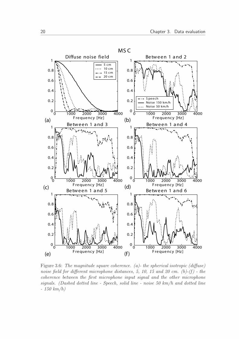
The space-time correlation functions for omnidirectional receivers in spher-ically isotropic (diffuse) noise field environments are well known, i.e. a largenumber of uncorrelated sources placed inside a hypothetic spherical shell at alarge radius. The coherence function of a diffuse noise field of two sampled sig-nals recorded with omnidirectional microphones is given by [17][18]
Cdifflm(f) =
sin2(2π fcdlm)
(2π fcdlm)2
(3.3)
where dlm denotes distance between the microphones indexed l and m, c thespeed of sound. In figure 3.6(a) the Cdiffuse are plotted for microphone distancesdlm of 5, 10, 15 and 20cm.
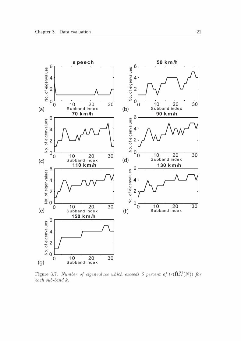
The speech signal, spacial close to the array, have a strong direct path signal.The coherence function for the speech signal in figure 3.6 (b)-(f), marked asdashed-dotted line, seems to have high correlation between the microphones.The speech signal impinging on the array should therefore have one dominatingeigenvalue as long as the space between each array element is sufficient. Figure3.7 shows the number of eigenvalue, for subband k, that exceeds 5 percent oftr(R
(k)xx (N)). The speech signal, shown i (a), have a dominated eigenvalue for
almost every sub-bands, and could be seen as a point source.From figure 3.6 (b)-(f) we may conclude that the noise field is incoherent,
close to a diffuse noise environment. At higher speeds, at frequencies between1-1.5kHz, the noise field become more diffuse. The spacial resolution is poorat low frequencies. Since the correlation is high at low frequencies there is fewdominating eigenvalues, see 3.7(b)-(g), while for higher frequencies the numberof eigenvalues increase.
It can be shown that the optimal weights for a near-field point source withthe array response vector a
(f)s in a diffuse noise situation are given by [19]
w(f)opt = R(f)−1
nn a(f)∗s (3.4)
where ∗ denotes a conjugation and Rnn is the correlation matrix of the spher-ical isotropic noise field where the correlation between element l and m can becalculated from
R(f)nlnm
= σ2nCdifflm
(f). (3.5)
20 Chapter 3. Data evaluation
0 1000 2000 3000 40000
0.2
0.4
0.6
0.8
1 Diffuse noise fie ld
F re que ncy [Hz ]0 1000 2000 3000 4000
0
0.2
0.4
0.6
0.8
1Be tw e e n 1 a nd 2
F re que ncy [Hz ]
0 1000 2000 3000 40000
0.2
0.4
0.6
0.8
1Be tw e e n 1 a nd 3
F re que ncy [Hz ]0 1000 2000 3000 4000
0
0.2
0.4
0.6
0.8
1Be tw e e n 1 a nd 4
F re que ncy [Hz ]
0 1000 2000 3000 40000
0.2
0.4
0.6
0.8
1Be tw e e n 1 a nd 5
F re que ncy [Hz ]0 1000 2000 3000 4000
0
0.2
0.4
0.6
0.8
1Be tw e e n 1 a nd 6
F re que ncy [Hz ]
5 cm
10 cm
15 cm
20 cm
S pe e ch
Noise 150 km/h
Noise 50 km/h
MS C
(a) (b)
(c) (d)
(e) (f )
Figure 3.6: The magnitude square coherence. (a)- the spherical isotropic (diffuse)noise field for different microphone distances, 5, 10, 15 and 20 cm. (b)-(f) - thecoherence between the first microphone input signal and the other microphonesignals. (Dashed dotted line - Speech, solid line - noise 50 km/h and dotted line- 150 km/h)
Chapter 3. Data evaluation 21
s peech 50 k m /h
70 k m /h 90 k m /h
110 k m /h
10 20 300
2
4
6130 k m /h
S ubband index
No
. o
f e
ige
nv
alu
es
150 k m /h
0
10 20 30
2
4
6
S ubband index
No
. o
f e
ige
nv
alu
es
00
10 20 30
2
4
6
S ubband index
No
. o
f e
ige
nv
alu
es
0
10 20 300
2
4
6
S ubband index
No
. o
f e
ige
nv
alu
es
0 10 20 300
2
4
6
S ubband index
No
. o
f e
ige
nv
alu
es
0
10 20 300
2
4
6
S ubband index
No
. o
f e
ige
nv
alu
es
0 10 20 300
2
4
6
S ubband index
No
. o
f e
ige
nv
alu
es
0(a)
(d)
(g)
(c)
(b)
(f )(e)
0
Figure 3.7: Number of eigenvalues which exceeds 5 percent of tr(R(k)xx (N)) for
each sub-band k.

22 Chapter 3. Data evaluation
Chapter 4
Implementation
4.1 The speech enhancement beamformer
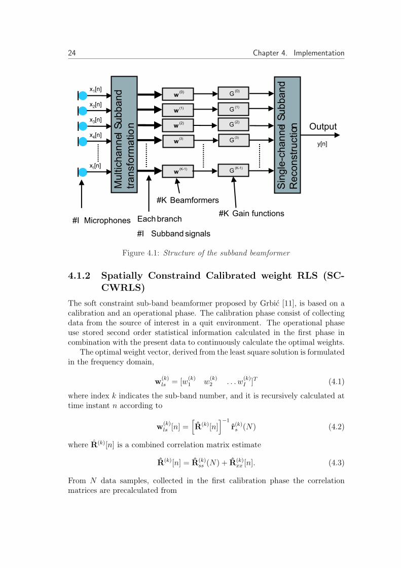
There are some consideration when designing a beamformer for the motorcyclehelmet environment. The placement of the microphones are limited inside thehelmet and depending on the driver the distance between the mouth and themicrophone array will differ but assumed to be fixed while driving. Describingthe environment by a priori model would be a very difficult task whereas amethod using a calibration signal is preferable. The beamformer algorithm needsto be able to adapt to the non-stationary noise field. An suitable algorithm is thespatially constraint sub-band beamformer [12] in a combination with the temporalspeech booster algoritm [3]. The overall speech enhancement beamformer systemare depicted in figure 4.1.
4.1.1 Filterbank
In this work a multichannel uniform over-sampled DFT filterbank is adopted.A modulated filterbank combined with the polyphase structure is used to re-duce the computational cost which also provides a great design simplicity. Inorder to reduce the aliasing effect the sub-band decomposition of K sub-bands ismade over-sampled by using a decimation factor of K
2. The transformation and
reconstruction filters are implemented by the method described in [13], whichminimizes the in-band and output aliasing errors that occurs in the analysis andsynthesis filter design. These aliasing effects are due to non-ideal frequency re-sponses of the filters in the filterbank.
23
24 Chapter 4. Implementation
Multic
hannelS
ubband
tra
nsfo
rma
tio
n
Each branch
#I Subband signals
#K Beamformers
Sin
gle
-channel
Subband
Re
co
nstr
uction
#I Microphones
Output
x1[n]
x2[n]
x3[n]
x4[n]
xI[n]
y[n]
w
w
w
w
w(K-1)
(3)
(2)
(1)
(0) G
G
G
G
G(K-1)
(3)
(2)
(1)
(0)
#K Gain functions
Figure 4.1: Structure of the subband beamformer
4.1.2 Spatially Constraind Calibrated weight RLS (SC-CWRLS)
The soft constraint sub-band beamformer proposed by Grbic [11], is based on acalibration and an operational phase. The calibration phase consist of collectingdata from the source of interest in a quit environment. The operational phaseuse stored second order statistical information calculated in the first phase incombination with the present data to continuously calculate the optimal weights.
The optimal weight vector, derived from the least square solution is formulatedin the frequency domain,
w(k)ls = [w
(k)1 w
(k)2 . . . w
(k)I ]T (4.1)
where index k indicates the sub-band number, and it is recursively calculated attime instant n according to
w(k)ls [n] =
[R(k)[n]
]−1
r(k)s (N) (4.2)
where R(k)[n] is a combined correlation matrix estimate
R(k)[n] = R(k)ss (N) + R(k)
xx [n]. (4.3)
From N data samples, collected in the first calibration phase the correlationmatrices are precalculated from
Chapter 4. Implementation 25
R(k)ss (N) =
1
N
N−1∑m=0
s(k)[m]s(k)[m]H (4.4)
r(k)s (N) =
1
N
N−1∑m=0
s(k)[m]s(k)[m]∗ (4.5)
wheres(k)[m] = [s
(k)1 [m] s
(k)2 [m] . . . s
(k)I [m]]T (4.6)
and where each signal, s(k)i [m], is the received data at the i:th microphone when
only the source signal of interest is active, for sub-band k.The observed data correlation matrix is given by
R(k)xx [n] =
n−1∑
l=0
λn−1−lx(k)[l]x(k)[l]H (4.7)
where x(k)[l] is the input vector for sub-band k, at time instant l and where λis a weighting factor. The inverse of (4.3) is effectively updated, recursively forevery time instant [11].
We propose the spatial constraints which make sure that sources originatingfrom the desired spatial location, calculated from the calibration data, maintainsa constant gain [12]. The weight vector then becomes
w(k)new[n] =
w(k)ls [n]∣∣∣w(k)
ls
H[n]r
(k)s (N)
∣∣∣P (k)(N) (4.8)
where P (k)(N) is a scalar to compensate for the power of the desired signal fromthe calibration phase
P (k)(N) =1
N
N−1∑m=0
s(k)[m]∗s(k)[m]. (4.9)
4.1.3 Adaptive gain equalizer
For each sub-band, an adaptive weighting function, called a gain function, amplifythe signal when speech is active. The gain function, G(k)[n], estimates a shorttime SNR, by calculating the ratio of a short term exponential magnitude averageA(k)[n], based on
∣∣x(k)[n]∣∣ and an estimate of the noise floor level, A(k)[n]. The
gain function for sub-band, k, is given by
G(k)[n] =
(A(k)[n]
A(k)[n]
)p
(4.10)
26 Chapter 4. Implementation
where p controls the amount of gain applied to each of the sub-band signals. Theshort term average in sub-band k, A(k)[n], is calculated as
A(k)[n] = (1− η(k))A(k)[n− 1] + η(k)|x(k)[n]| (4.11)
where η(k) is a smoothing factor and can be estimated by
η(k) =1
T(k)s Fs
(4.12)
where Fs is the sampling frequency and T(k)s is a time constant. A(k)[n], is calcu-
lated according to
A(k)[n] =
{(1 + ζ(k))A(k)[n− 1] if A(k)[n− 1] 6 A(k)[n]
A(k)[n] if A(k)[n− 1] < A(k)[n](4.13)
where ζ(k) is a small positive constant controlling how fast the noise floor levelestimate in sub-band k will adapt to changes in the noise environment. To ensurethat the gain function does not become excessively large a gain limiter is alsoincluded.
Chapter 5
Evaluations
5.1 Parameters settings
The uniform over-sampled DFT filterbank decompose the received array signalinto 64 sub-band signals. The length of the prototype filter is set to 512. Eachsub-band has one tap filters, recursively calculated by spatially constraint CW-RLS algorithm. The step-size are set to α = 0.005 and the weighting factorλ = 0.9. An evaluation of parameter settings for CW-RLS is found in [20].
For the speech booster a suitable time factor Ts is 30 ms and with the samplefrequency of Fs = 8000 Hz the smoothing factor η = 0.0042 is calculate by usingequation (4.12). The noise floor level is set to ζ = 1e−6, the exponential gainfactor constant p = 1 and the upper bound for the gain function G[n] is 10 dB.
5.2 Output SNR
In order to evaluate the performance of the system there are four solutions calcu-lated for each motorcycle speed. Each of the algorithms are either working alone,i.e. (1) the speech booster representing the single microphone solution and (2)the SCCWRLS representing the multi microphone array system, and (3) a com-bination of these two system working together and finally (4) the (non-adaptive)optimal subband wiener solution according to equation 2.10.
The signal to noise ratio for each of these four cases are shown in table 2. Theinput signal is the received signal from the reference microphone, i.e. the fourthmicrophone in the array. These results are also presented graphically in figure5.1.
27

28 Chapter 5. Evaluations
50 70 90 110 130 150−10
−5
0
5
10
15
20
25
SNR
speeds [km/h]
[dB
]
Input signal(1) SB (2) SCCWRLS(3) Combined(4) Wiener
Figure 5.1: SNR at different speeds for the received input signal on the referencemicrophone, (1) - Speech Booster, (2) - SCCWRLS, (3) - both methods combinedand (4) the subband Wiener soultion.
SNR [dB] Speed [km/h]
50 70 90 110 130 150
Input 17.2 10.1 3.9 -0.5 -4.5 -9.7(1) Speech Booster 20.2 13.0 6.7 2.0 -3.2 -9.0(2) SCCWRLS 19.7 13.0 8.4 3.9 2.6 -1.4(3) Combined 21.6 15.1 11.3 6.5 5.5 1.7(4) Wiener 21.3 14.9 10.9 8.1 6.8 3.7
Table 2. SNR at different speeds for the received input signal on the referencemicrophone, (1) the Speech Booster, (2) the SCCWRLS working alone and (3)both methods combined and (4) the subband Wiener solution
Chapter 5. Evaluations 29
For high SNR, i.e. low velocities, the Speech Booster enhances the speechsignal successfully. For negative SNR, which corresponds to speeds above 110km/h, the Speech Booster solution have a high noise floor and the difference issmoothed out which results in a reduced amplification of the signal. On the otherhand, the array based beamformer works more efficiently to suppress the noisefor low SNR and consequently it leads to an increased SNR.
By adding the Speech booster in cascade with the SCCWRLS as shown inthe system overview (figure 4.1) the working range of the Speech Boosters isincreased such that it operates successfully also at higher speeds, which can beseen in figure 5.1, and consequently the total SNR performance is significatlyincreased at all speeds.
5.3 Noise suppression and Speech distortion
The performance evaluation is based on two measures, the distortion caused bythe beamforming filters measured by the spectral deviation between the beam-former output and the source signal, and the noise suppression.
5.3.1 Performance measures
In order to measure the performance, the normalized distortion quantity, D, isintroduced as
D =1
2π
∫ π
−π
|CdPys(ω)− Pxs(ω)|dω (5.1)
where ω = 2πf , and f is normalized frequency. The constant, Cd, is defined as
Cd =
∫ π
−πPxs(ω)dω∫ π
−πPys(ω)dω
(5.2)
where Pxs(ω) is a PSD estimate of a single sensor observation and Pys(ω) isthe PSD estimate of the beamformer output, when the source signal is activealone. The constant Cd normalize the mean output spectral power to that ofthe single sensor spectral power. The single sensor observation is chosen as thereference microphone observation, i.e. microphone number four in the array.The mean output spectral power of the reference signal is normalized to one.The distortion measure in Eq. 5.1, is the mean output spectral power deviationfrom the observed single sensor spectral power. Ideally, the distortion is zero. Inorder to measure the noise suppression the normalized noise suppression quantity,N , is introduced as
N = CS
∫ π
−πPxN
(ω)dω∫ π
−πPyN
(ω)dω(5.3)
30 Chapter 5. Evaluations
where
CS =1
Cd
(5.4)
and where, PyN(ω) and PxN
(ω) are PSD of the beamformer output and the refer-ence sensor observation, respectively, when the surrounding noise is active alone.The noise suppression measures are normalized to the amplification/attenuationcaused by the beamformer to the reference sensor observation when the sourcesignal is active alone, i.e. if the beamformer attenuates the source signal bya specific amount, the noise suppression quantities are reduced with the sameamount.
5.3.2 Noise suppression
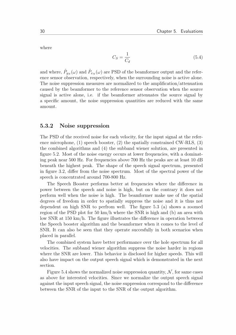
The PSD of the received noise for each velocity, for the input signal at the refer-ence microphone, (1) speech booster, (2) the spatially constrained CW-RLS, (3)the combined algorithms and (4) the subband wiener solution, are presented infigure 5.2. Most of the noise energy occurs at lower frequencies, with a dominat-ing peak near 500 Hz. For frequencies above 700 Hz the peaks are at least 10 dBbeneath the highest peak. The shape of the speech signal spectrum, presentedin figure 3.2, differ from the noise spectrum. Most of the spectral power of thespeech is concentrated around 700-800 Hz.
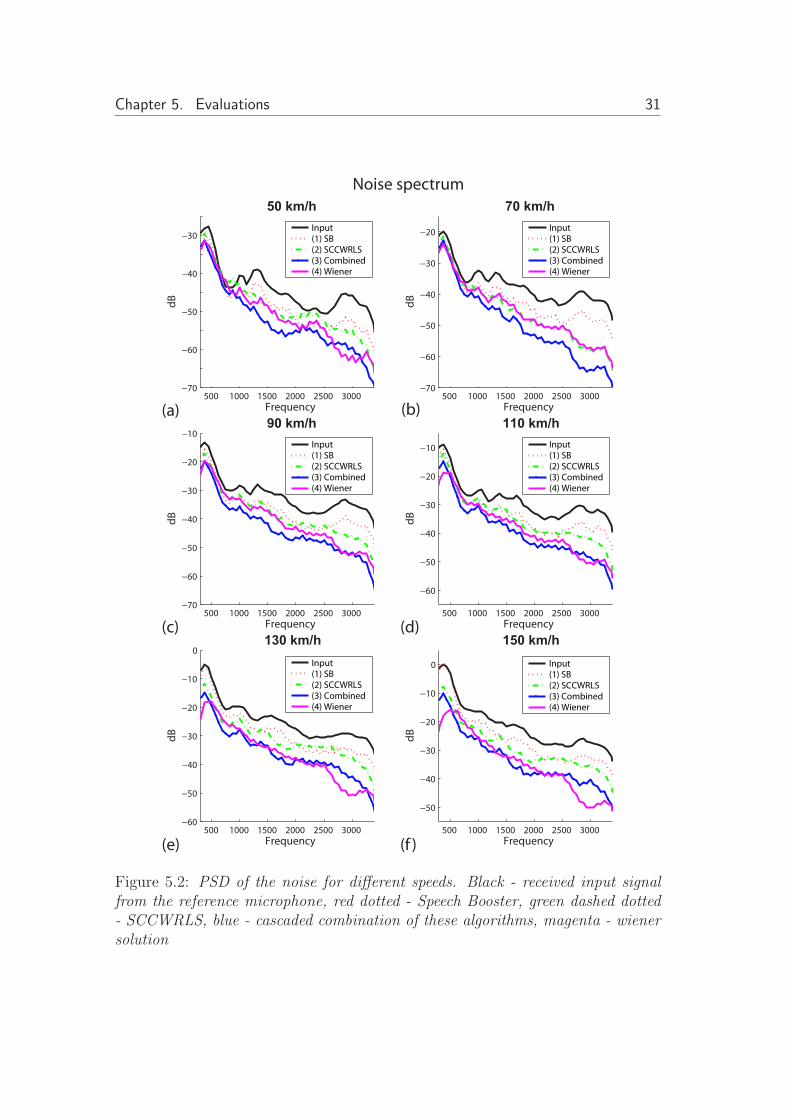
The Speech Booster performs better at frequencies where the difference inpower between the speech and noise is high, but on the contrary it does notperform well when the noise is high. The beamformer make use of the spatialdegrees of freedom in order to spatially suppress the noise and it is thus notdependent on high SNR to perfrom well. The figure 5.3 (a) shows a zoomedregion of the PSD plot for 50 km/h where the SNR is high and (b) an area withlow SNR at 150 km/h. The figure illustrates the difference in operation betweenthe Speech booster algorithm and the beamformer when it comes to the level ofSNR. It can also be seen that they operate succesfully in both scenarios whenplaced in parallel.
The combined system have better performance over the hole spectrum for allvelocities. The subband wiener algorithm suppress the noise harder in regionswhere the SNR are lower. This behavior is disclosed for higher speeds. This willalso have impact on the output speech signal which is demonstrated in the nextsection.
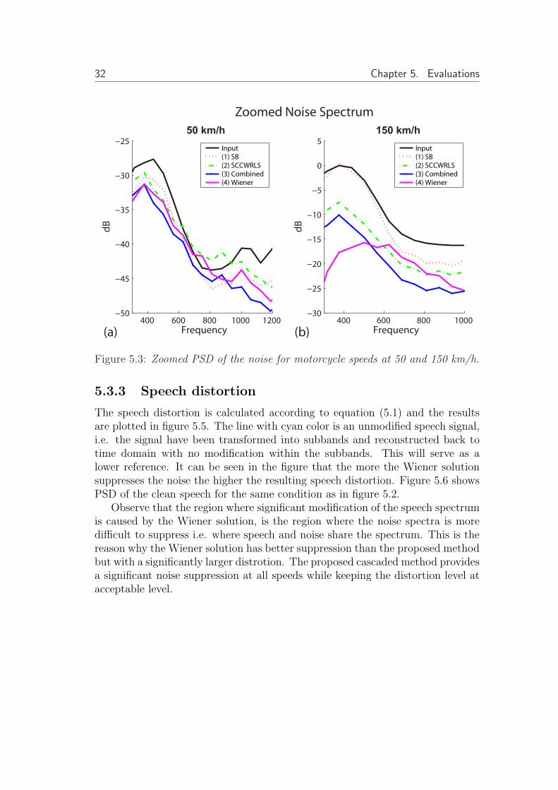
Figure 5.4 shows the normalized noise suppression quantity, N , for same casesas above for interested velocities. Since we normalize the output speech signalagainst the input speech signal, the noise suppression correspond to the differencebetween the SNR of the input to the SNR of the output algorithm.
Chapter 5. Evaluations 31
500 1000 1500 2000 2500 3000−70
−60
−50
−40
−30
Frequency
dB
50 km/h
500 1000 1500 2000 2500 3000−70
−60
−50
−40
−30
−20
Frequencyd
B
70 km/h
500 1000 1500 2000 2500 3000−70
−60
−50
−40
−30
−20
−10
Frequency
dB
90 km/h
500 1000 1500 2000 2500 3000
−60
−50
−40
−30
−20
−10
Frequency
dB
110 km/h
500 1000 1500 2000 2500 3000−60
−50
−40
−30
−20
−10
0
Frequency
dB
130 km/h
500 1000 1500 2000 2500 3000
−50
−40
−30
−20
−10
0
Frequency
dB
150 km/h
Noise spectrum
(a)
(c)
(b)
(f )(e)
(d)
Input
(1) SB
(2) SCCWRLS
(3) Combined
(4) Wiener
Input
(1) SB
(2) SCCWRLS
(3) Combined
(4) Wiener
Input
(1) SB
(2) SCCWRLS
(3) Combined
(4) Wiener
Input
(1) SB
(2) SCCWRLS
(3) Combined
(4) Wiener
Input
(1) SB
(2) SCCWRLS
(3) Combined
(4) Wiener
Input
(1) SB
(2) SCCWRLS
(3) Combined
(4) Wiener
Figure 5.2: PSD of the noise for different speeds. Black - received input signalfrom the reference microphone, red dotted - Speech Booster, green dashed dotted- SCCWRLS, blue - cascaded combination of these algorithms, magenta - wienersolution
32 Chapter 5. Evaluations
400 600 800 1000 1200−50
−45
−40
−35
−30
−25
Frequency
dB
50 km/h
400 600 800 1000−30
−25
−20
−15
−10
−5
0
5
Frequency
dB
150 km/h
Zoomed Noise Spectrum
(a) (b)
Input
(1) SB
(2) SCCWRLS
(3) Combined
(4) Wiener
Input
(1) SB
(2) SCCWRLS
(3) Combined
(4) Wiener
Figure 5.3: Zoomed PSD of the noise for motorcycle speeds at 50 and 150 km/h.
5.3.3 Speech distortion
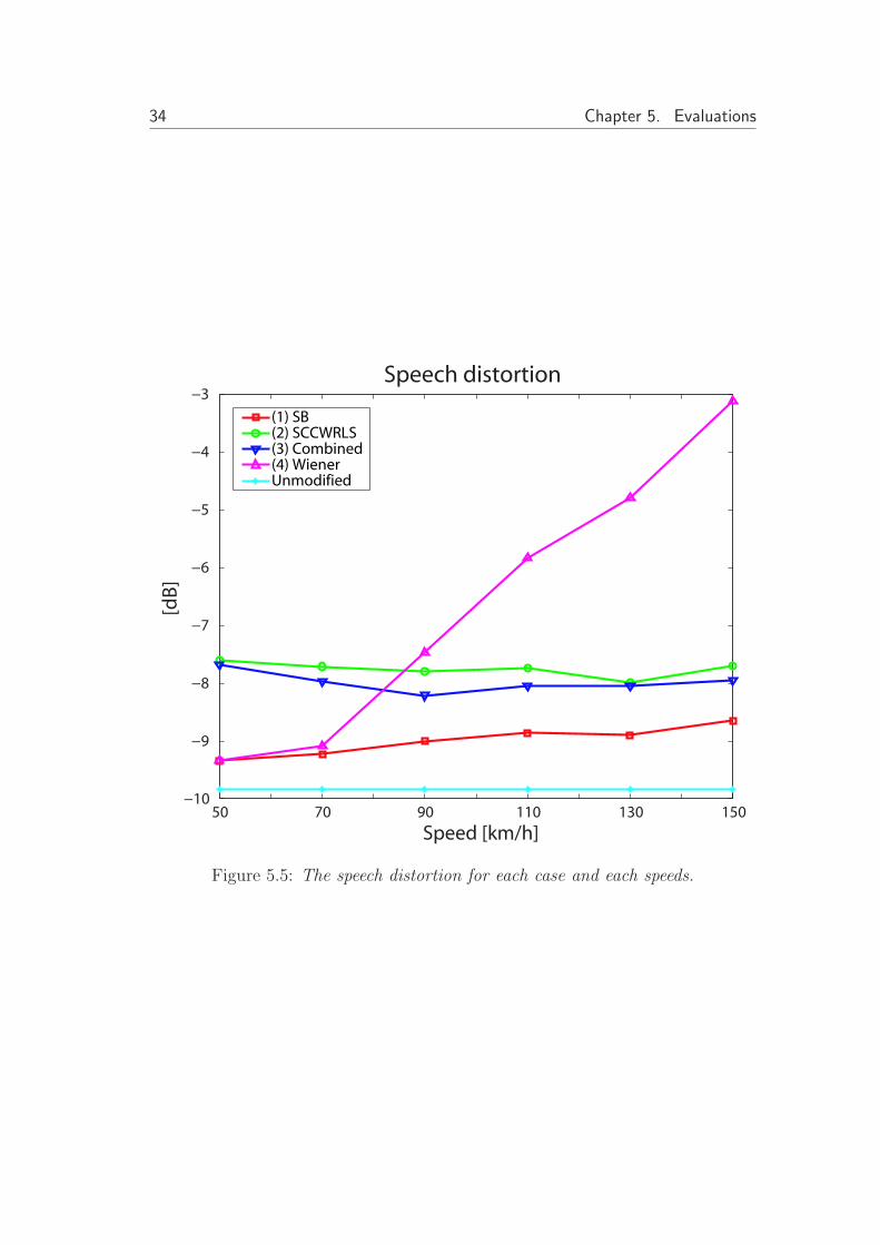
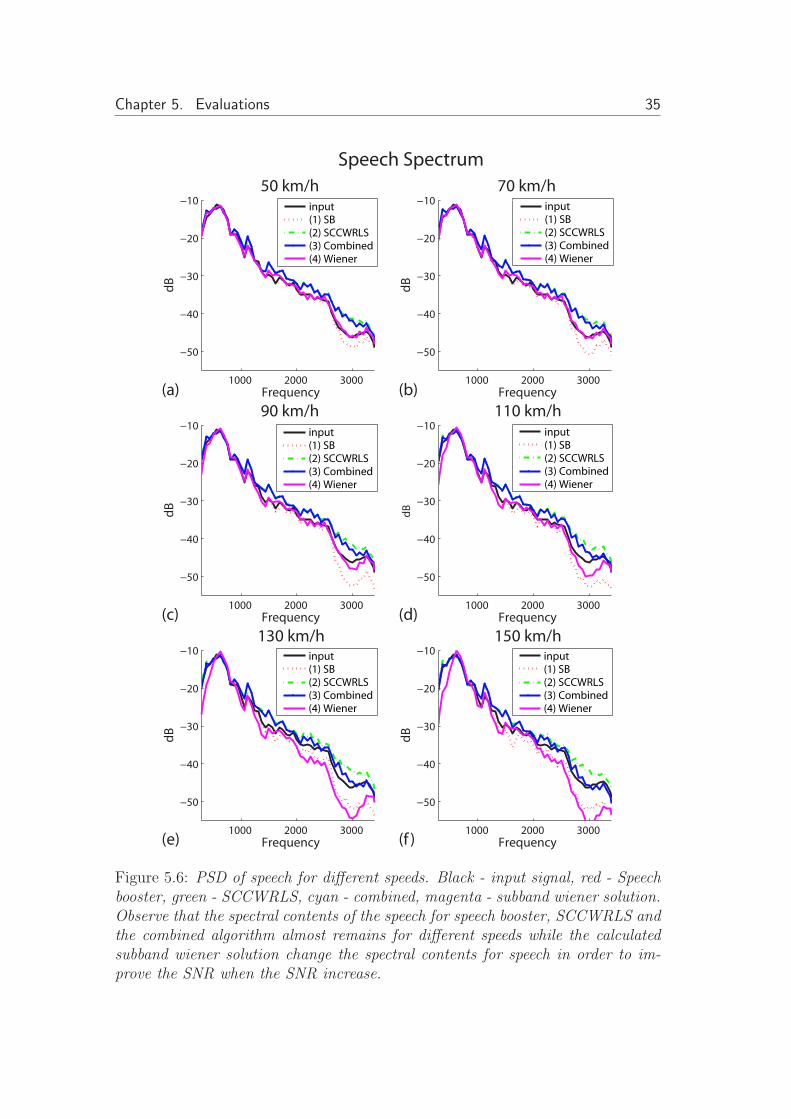
The speech distortion is calculated according to equation (5.1) and the resultsare plotted in figure 5.5. The line with cyan color is an unmodified speech signal,i.e. the signal have been transformed into subbands and reconstructed back totime domain with no modification within the subbands. This will serve as alower reference. It can be seen in the figure that the more the Wiener solutionsuppresses the noise the higher the resulting speech distortion. Figure 5.6 showsPSD of the clean speech for the same condition as in figure 5.2.
Observe that the region where significant modification of the speech spectrumis caused by the Wiener solution, is the region where the noise spectra is moredifficult to suppress i.e. where speech and noise share the spectrum. This is thereason why the Wiener solution has better suppression than the proposed methodbut with a significantly larger distrotion. The proposed cascaded method providesa significant noise suppression at all speeds while keeping the distortion level atacceptable level.
Chapter 5. Evaluations 33
50 70 90 110 130 1500
2
4
6
8
10
12
14
speeds [km/h]
[dB
]
Noise supression
(1) SB(2) SCCWRLS(3) Combined(4) Winer
Figure 5.4: Noise suppression for different velocities.
34 Chapter 5. Evaluations
50 70 90 110 130 150−10
−9
−8
−7
−6
−5
−4
−3Speech distortion
Speed [km/h]
[dB
]
(1) SB(2) SCCWRLS(3) Combined(4) WienerUnmodified
Figure 5.5: The speech distortion for each case and each speeds.
Chapter 5. Evaluations 35
1000 2000 3000
−50
−40
−30
−20
−10
Frequency
dB
50 km/hinput
(1) SB
(2) SCCWRLS
(3) Combined
(4) Wiener
1000 2000 3000
−50
−40
−30
−20
−10
Frequencyd
B
70 km/h
1000 2000 3000
−50
−40
−30
−20
−10
Frequency
dB
90 km/h
1000 2000 3000
−50
−40
−30
−20
−10
Frequency
dB
110 km/h
1000 2000 3000
−50
−40
−30
−20
−10
Frequency
dB
130 km/h
1000 2000 3000
−50
−40
−30
−20
−10
Frequency
dB
150 km/h
Speech Spectrum
(a) (b)
(c)
(e)
(d)
(f )
input
(1) SB
(2) SCCWRLS
(3) Combined
(4) Wiener
input
(1) SB
(2) SCCWRLS
(3) Combined
(4) Wiener
input
(1) SB
(2) SCCWRLS
(3) Combined
(4) Wiener
input
(1) SB
(2) SCCWRLS
(3) Combined
(4) Wiener
input
(1) SB
(2) SCCWRLS
(3) Combined
(4) Wiener
Figure 5.6: PSD of speech for different speeds. Black - input signal, red - Speechbooster, green - SCCWRLS, cyan - combined, magenta - subband wiener solution.Observe that the spectral contents of the speech for speech booster, SCCWRLS andthe combined algorithm almost remains for different speeds while the calculatedsubband wiener solution change the spectral contents for speech in order to im-prove the SNR when the SNR increase.

36 Chapter 5. Evaluations
Chapter 6
Summary and conclusions
A case study of speech enhancement in a helmet communication on a movingmotorcycle has been presented. A microphone array with 6 elements was placedonto the visor inside the helmet. Driving conditions at speeds of 50, 70, 90,110, 130 and 150 km/h have been analyzed and results show that the noisefield dominates at high speeds. The noise mainly consists of a spatially widelyspread wind noise penetrating through the helmet, together with engine andtire noise. The range of signal to noise ratios (SNR:s) reaches from about 17dB at 50 km/h to as low as -9 dB at 150 km/h. In order to provide meansfor a speech conversation at these high speeds, an adaptive system for speechenhancement/noise reduction have been proposed and evaluated.
A polyphase structure of a uniform DFT filterbank is used to transform theinput signals into 64 subband signals. A spatially soft constrained subband beam-former combined with a SNR dependent single microphone solution form theadaptive algorithm used to reduce the noise and the system thereby enhances thespeech signal. The beamformer makes use of a calibrated signal gathered in situfrom the speaker’s position. This calibration procedure efficiently captures theacoustical properties in the actual environment. The algorithm does not needto rely on any speech activity detection and therefore the problems of faultydetection are avoided.
Evaluation of the beamformer and the single microphone algorithm, bothas either parts by them selves and as a cascaded structure, together with theoptimal subband Wiener solution is presented. The beamformer works moreefficiently on suppressing the noise when the SNR is low while the single channelalgorithm success heavily depends upon a high SNR. It is shown that a cascadedcombination of the calibrated subband beamforming technique together with thesingle channel solution outperforms either one by it self, and provides good resultsat all noise levels. The Wiener solution increases the SNR at high speeds slightlymore than the proposed system but at the cost of an increased speech distortion.The proposed system suppresses the noise and enhances the speech signal whilekeeping the speech distortion low.
37
38 Chapter 6. Summary and conclusions
Appendix A
Spectrograms
39
40 Appendix A. Spectrograms
Fre
qu
en
cy
[H
z]
Fre
qu
en
cy
[H
z]
Fre
qu
en
cy
[H
z]
Fre
qu
en
cy
[H
z]
Time [s]
Time [s] Time [s]
Time [s]
Spectrogram - 50 km/h
Input signal Speech booster
SCCWRLS Combined
(a) (b)
(d)(c)
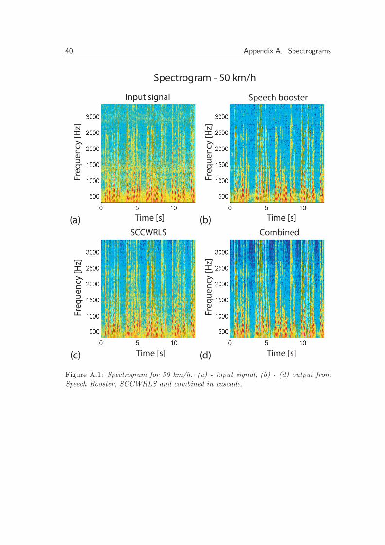
Figure A.1: Spectrogram for 50 km/h. (a) - input signal, (b) - (d) output fromSpeech Booster, SCCWRLS and combined in cascade.
Appendix A. Spectrograms 41
Fre
qu
en
cy
[H
z]
Fre
qu
en
cy
[H
z]
Fre
qu
en
cy
[H
z]
Fre
qu
en
cy
[H
z]
Time [s]
Time [s] Time [s]
Time [s]
Spectrogram - 70 km/h
Input signal Speech booster
SCCWRLS Combined
(a) (b)
(d)(c)
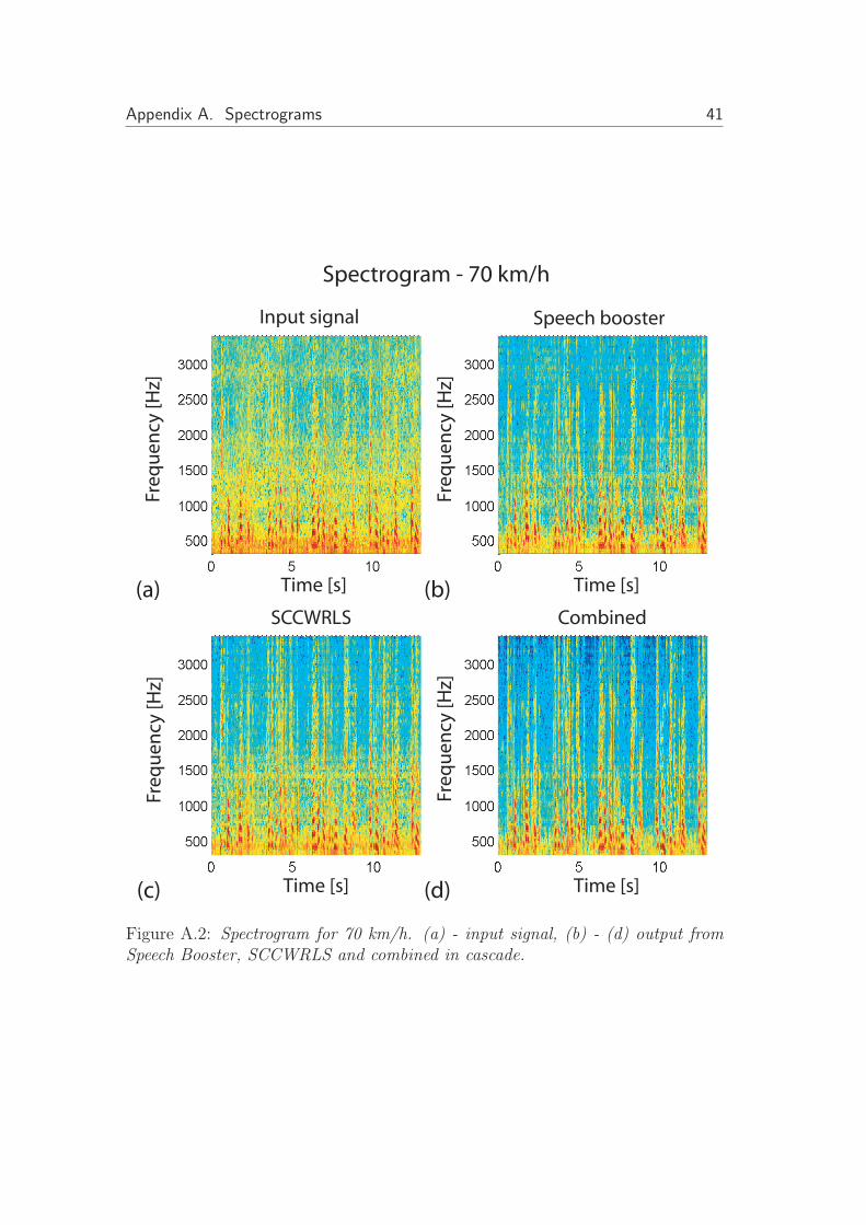
Figure A.2: Spectrogram for 70 km/h. (a) - input signal, (b) - (d) output fromSpeech Booster, SCCWRLS and combined in cascade.

42 Appendix A. Spectrograms
Fre
qu
en
cy
[H
z]
Fre
qu
en
cy
[H
z]
Fre
qu
en
cy
[H
z]
Fre
qu
en
cy
[H
z]
Time [s]
Time [s] Time [s]
Time [s]
Spectrogram - 90 km/h
Input signal Speech booster
SCCWRLS Combined
(a) (b)
(d)(c)
Figure A.3: Spectrogram for 90 km/h. (a) - input signal, (b) - (d) output fromSpeech Booster, SCCWRLS and combined in cascade.
Appendix A. Spectrograms 43
Fre
qu
en
cy
[H
z]
Fre
qu
en
cy
[H
z]
Fre
qu
en
cy
[H
z]
Fre
qu
en
cy
[H
z]
Time [s]
Time [s] Time [s]
Time [s]
Spectrogram - 110 km/h
Input signal Speech booster
SCCWRLS Combined
(a) (b)
(d)(c)
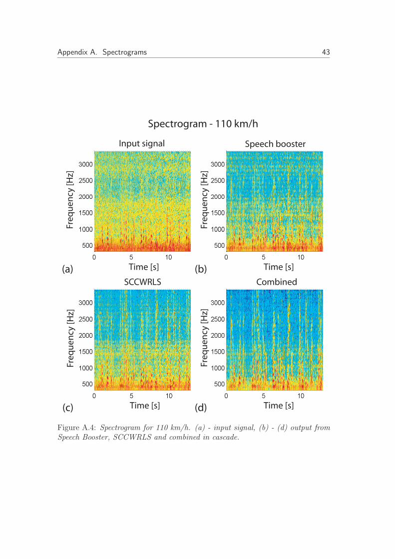
Figure A.4: Spectrogram for 110 km/h. (a) - input signal, (b) - (d) output fromSpeech Booster, SCCWRLS and combined in cascade.
44 Appendix A. Spectrograms
Fre
qu
en
cy
[H
z]
Fre
qu
en
cy
[H
z]
Fre
qu
en
cy
[H
z]
Fre
qu
en
cy
[H
z]
Time [s]
Time [s] Time [s]
Time [s]
Spectrogram - 130 km/h
Input signal Speech booster
SCCWRLS Combined
(a) (b)
(d)(c)
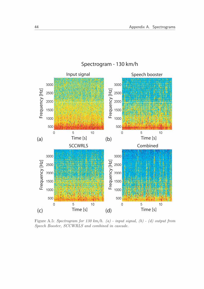
Figure A.5: Spectrogram for 130 km/h. (a) - input signal, (b) - (d) output fromSpeech Booster, SCCWRLS and combined in cascade.
Appendix A. Spectrograms 45
Fre
qu
en
cy
[H
z]
Fre
qu
en
cy
[H
z]
Fre
qu
en
cy
[H
z]
Fre
qu
en
cy
[H
z]
Time [s]
Time [s] Time [s]
Time [s]
Spectrogram - 150 km/h
Input signal Speech booster
SCCWRLS Combined
(a) (b)
(d)(c)
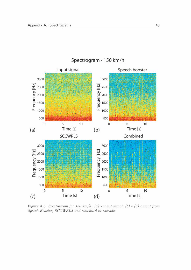
Figure A.6: Spectrogram for 150 km/h. (a) - input signal, (b) - (d) output fromSpeech Booster, SCCWRLS and combined in cascade.
46 Appendix A. Spectrograms
Bibliography
[1] S. F. Boll, “Suppression of accustic noise in speech using spectral subtrac-tion,” IEEE trans. Acoust. Speech and Sig. Proc.,, vol. ASSP-27, pp. 113-120,April 1979.
[2] J. R. Deller Jr., J. G. Proakis, and J. H. L. Hansen, Discrete time processingof speech signals, Macmillan Publishing Company, 1993.
[3] N. Wersterlund,“Applied Speech Enhancement for Personal Communication,Blekinge institute of Technology, ISBN 91-7295-020-x, Maj 2003.
[4] M. Brandstein and D. Ward, Eds., Microphone Arrays: Signal ProcessingTechniques and Applications, Berlin: Springer Verlag, 2001.
[5] S. Nordholm, I. Claesson, and B. Bengtsson, “Adaptive Array Noise Sup-pression of Handsfree Speaker Input in Car,” IEEE trans. Vehicular Tech.,vol. 42, no.4, pp. 514-518, Nov 1993.
[6] B. Widrow and F.L. Luo,“Microphone arrays for hearing aids: Anoverview,”Speech communication, vol. 39,Iss. 1-2, pp. 139-146, Jan 2003.
[7] L. J. Griffiths and C. W. Jim,“An alternative approach to linearly con-strained adaptive beamforming,”IEEE trans. Antennas and Propagation,vol. AP-30, pp. 27-34, Jan 1982.
[8] J. Bitzer, K.U. Simmer, and K.D. Kammeyer, “Theoretical Noise ReductionLimits of the Generalized Sidelobe Canceler (GSC) for speech enhancement,”in IEEE International Conference on Acoustics, Speech and Signal Process-ing, vol. 5, pp. 2965-2968, May 1999.
[9] S. Affes and Y. Grenier, “A Signal Subspace Tracking Algorithm for Mi-crophone Array Processing of Speech,” IEEE International Conference onAcoustics, Speech and Signal Processing, vol. 5, no. 5, pp. 425–437, Septem-ber 1997.
[10] D. A. Florencio, and H. S. Malvar, “Multichannel Filtering for OptimumNoise Reduction in Microphone Arrays,” in IEEE International Conferenceon Acoustics, Speech and Signal Processing, vol. 1, pp. 197–200, May 2001.
47
48 Bibliography
[11] N. Grbic, “Optimal and Adaptive Subband Beamforming, Principles andApplications,” Dissertation Series No 01:01, ISSN:1650-2159, Blekinge In-stitute of Technology, 2001.
[12] P. Cornelius, Z. Yermeche, N. Grbic and I. Claesson, “A spatially constrainedsubband beamforming algorithm for speech enhancement ,”in IEEE SensorArray and Multichannel Signal Processing Workshop, july 2004. 1999.
[13] J. M. de Haan, N. Grbic, I. Claesson, and S. Nordholm, “Design of oversam-pled uniform dft filter banks with delay specifications using quadratic opti-mization,” IEEE International Conference on Acoustics, Speech and SignalProcessing, vol. VI, pp. 3633-3636, May 2001.
[14] D. Johnson and D. Dudgeon,“ Array Signal Processing - Concepts and Tech-niques,” Prentice Hall, 1993
[15] J.S. Bendat and A.G. Piersol, Measurment and Analysis of random Data,Wiley, 2000.
[16] J. Meyer and K. U. Simmer,“Multi-channel speech enhancement in a carenvironment using wiener filtering and spectral subtraction,”IEEE Interna-tional Conference on Acoustics, Speech and Signal Processing, vol. 2, pp.1167-1170, April 1997.
[17] H. Kuttruff, Room Acoustics, Elsevier Science,3rd edn., 1990.
[18] B.F. Cron and C.H. Sherman, “Spatial-Correlated Functions for Varios NoiseModels,”J. Acoust. Soc. Am., vol. 34, no. 11,pp. 1732-1736, 1962
[19] N. E. hudson, “Adaptive array principles”, Peter Peregrinus Ltd., 1981,ISBN 0-86341-247-5
[20] Z. Yermeche, “Subband Beamforming for Speech Enhancement in Hands-Free Communiction,” Dissertation Series No 2004:13, ISSN:1650-2140,Blekinge Institute of Technology, 2004.

Microphone Array System for Speech Enhancement in a MotorcycleHelmet
Per Cornelius, Nedelko Grbic, Ingvar Claesson
ISSN 1103-1581ISRN BTH-RES--05/05--SE
Copyright © 2005 by individual authorsAll rights reserved
Printed by Kaserntryckeriet AB, Karlskrona 2005