Citation: Alsheibi, A.Z.; Valavanis,

K.P.; Iqbal, A.; Aman, M.N. Speech

Enhancement Framework with Noise

Suppression Using Block Principal

Component Analysis. Acoustics 2022,

4, 441–459. https://doi.org/

10.3390/acoustics4020027

Academic Editor: Jian Kang

Received: 28 March 2022

Revised: 16 May 2022

Accepted: 17 May 2022

Published: 20 May 2022

Publisher’s Note: MDPI stays neutral

with regard to jurisdictional claims in

published maps and institutional affil-

iations.

Copyright: © 2022 by the authors.

Licensee MDPI, Basel, Switzerland.

This article is an open access article

distributed under the terms and

conditions of the Creative Commons

Attribution (CC BY) license (https://

creativecommons.org/licenses/by/

4.0/).

acoustics

Article

Speech Enhancement Framework with Noise SuppressionUsing Block Principal Component AnalysisAbdullah Zaini Alsheibi 1,* , Kimon P. Valavanis 1, Asif Iqbal 2 and Muhammad Naveed Aman 3,*

1 Department of Electrical and Computer Engineering, University of Denver, Denver, CO 80208, USA;kimon.valavanis@du.edu

2 Department of Electrical and Computer Engineering, National University of Singapore,Singapore 119077, Singapore; aiqbal@nus.edu.sg

3 School of Computing, University of Nebraska-Lincoln, Lincoln, NE 68588, USA* Correspondence: alsheibi-6080@hotmail.com (A.Z.A.); naveed.aman@unl.edu (M.N.A.)

Abstract: With the advancement in voice-communication-based human–machine interface technologyin smart home devices, the ability to decompose the received speech signal into a signal of interest andan interference component has emerged as a key requirement for their successful operation. Thesedevices perform their tasks in real time based on the received commands, and their effectivenessis limited when there is a lot of ambient noise in the area in which they operate. Most real-timespeech enhancement algorithms do not perform adequately well in the presence of high amounts ofnoise (i.e., low input-signal-to-noise ratio). In this manuscript, we propose a speech enhancementframework to help these algorithms in situations when the noise level in the received signal is high.The proposed framework performs noise suppression in the frequency domain by generating anapproximation of the noisy signals’ short-time Fourier transform, which is then used by the speechenhancement algorithms to recover the underlying clean signal. This approximation is performed byusing the proposed block principal component analysis (Block-PCA) algorithm. To illustrate efficacyof the proposed framework, we present a detailed performance evaluation under different noiselevels and noise types, highlighting the effectiveness of the proposed framework. Moreover, theproposed method can be used in conjunction with any speech enhancement algorithm to improve itsperformance under moderate to high noise scenarios.

Keywords: speech enhancement; principal component analysis; MMSE filtering; Block-PCA

1. Introduction

With the widespread acceptance of smart home devices and wireless networks enabledby voice-communication-based human–machine interface technologies, the need to im-prove the intelligibility and overall quality of the speech signal has become indispensable.The very first step in such voice-communication-based devices is to extract the signal/voiceof interest from the noise-contaminated received signal [1]. The contamination could consistof background noise, echoes, acoustic reverberation, or speech-like interference [1]. This iswhere speech enhancement algorithms can help. The goal of such algorithms is to reducethe noise or distortion present in the speech signal, thus improving its overall quality.

The use of multiple recording microphones can help ease the difficulty of speechenhancement. However, in the case of small-scale devices, such as hearing aids, size andcost limitations can hinder the inclusion of multiple microphones. Similarly, pre-recordedsingle-channel audio streams cannot benefit from these techniques either. As a result,single-channel speech enhancement techniques are employed in the pre-processing stepin low-cost and small-scale devices. These techniques perform either noise estimationor signal estimation (or both) to infer the clean signal from a noisy observation. In [2,3],voice activity detectors (VAD) are used to approximate frames of signal where the speakeris silent, and these frames are then used to estimate the noise spectrum. Once the noise

Acoustics 2022, 4, 441–459. https://doi.org/10.3390/acoustics4020027 https://www.mdpi.com/journal/acoustics

Acoustics 2022, 4 442

estimate is obtained, its spectrum is subtracted from the noisy spectrum, thus reducingthe overall noise level. These techniques, however, inherit the shortcomings associatedwith VAD usage, that is, they may fail if the frame size of the input signal is large or if thesignal-to-noise ratio (SNR) is low. Authors in [4] have proposed a backward blind sourceseparation structure implemented in subband domain using a least mean square algorithm,which leads to a reduction in speech distortion while maintaining speech intelligibility.In [5], the authors have proposed a hybrid technique with the combination of two-step,harmonic regeneration noise reduction and a comb filter. The proposed technique is shownto achieve better speech enhancement results in terms of general performance metricssuch as mean opinion score (MOS), mean square error (MSE), average segmental SNR(ASSNR), perceptual evaluation of speech quality (PESQ), and diagnostic rhyme test (DRT).The authors in [6] propose a semisoft threshold-based speech enhancement algorithmbased on noise coefficients determined by Teager energy-operated wavelet packets. Intheir simulation results, they have been shown to achieve better performance in terms ofstandard performance metrics such as MOS, MSE, ASSNR, PESQ, and so on.

Similarly, many signal estimation techniques, such as spectral subtraction [7–11], weinerfiltering [12–14], and minimum mean square error (MMSE) estimation-based methods [15–20],have been proposed. Out of these, the spectral subtraction methods are the most computa-tionally efficient. They operate by estimating the noise spectrum from the noisy speech signaland then recovering the clean signal by subtracting the estimated noise spectrum from thenoisy one. These methods generally perform well; however, so-called musical noise mightappear in their recovered signal. On the other hand, the MMSE-based methods are free fromthe issue of musical noise. The authors in [15] derive and use a filter using the minimummean square error–short-time spectral amplitude (MMSE-STSA) estimator based on the costfunction minimizing the mean squared error of the short-time amplitude of the spectrum.The authors in [16] use a perceptually motivated cost function minimizing the mean squarederror between the logarithmic spectral amplitude of the clean and enhanced speech signal,whereas [17] proposes an adaptive β-order MMSE estimator to design a filter. The designedfilter is then used to enhance the signal frequencies, leading to a clean speech signal.

Based on our literature review, one key issue with most speech enhancement algo-rithms is their susceptibility to the input SNR levels. Under moderate to high SNR, theirenhancement results are objectively better; however, under low to poor SNR conditions,these methods fail altogether. Here, we consider SNR levels ≤ zero as low and those abovezero as medium. For example, most of the papers have reported their experimental resultsover the input SNR range of −5 dB onwards, as shown in Table 1. The method in [6] doesevaluate from−15 dB SNR and show slight improvement as the SNR is improved. However,they only report results on the ‘Car’ noise case from NOIZEUS [21], which is an easy-to-usedataset for speech quality improvement. In this manuscript, we aim to remedy this situationby introducing a pre-processing step implemented in the frequency domain that reduces theoverall noise level of the signal, resulting in improvement of SNR. This pre-processed signalcan then be passed to any other speech enhancement algorithms as usual, leading to superiorresults. The pre-processing step involves a variation of the principal component analysis(PCA) technique, termed Block-PCA, which operates on blocks of the short-time Fouriertransform (STFT) of the noisy signal to generate an STFT approximation by suppressing thenoise level present in the signal.

Acoustics 2022, 4 443

Table 1. Publications with performance evaluations on input SNR.

Reference Input SNR Range in dB

[3] −3 dB onwards[5] −5 dB onwards[6] −15 dB onwards

[10] 0 dB onwards[11] −5 dB onwards[20] −3 dB onwards[22] 1 dB onwards[23] 0 dB onwards[24] 0 dB onwards[25] 0 dB onwards

Principal component analysis (PCA) is one of the most utilized feature extraction anddimensionality reduction techniques in all of data science and engineering, particularlyin image and signal processing, pattern extraction and recognition, and machine learning,as well as other exploratory data analysis [26,27]. It has been extensively used in variousapplications, for example, image noise estimation [28], denoising [29], speech enhance-ment [25,30,31], video watermarking [32], video and image classification [33], analysis offunctional magnetic resonance imaging data [34,35], analysis of local growth policy in theperspective of institutional governance [36], and face recognition [37].

Consider a dataset consisting of p-dimensional variables y ∈ Rp sampled from anunknown p-dimensional subspace. For such a dataset, PCA can be used to generatean orthogonal projection onto a lower-dimensional subspace, typically named principalsubspace [38], which can explain most of the variance (statistical information) of the data.These orthogonal basis vectors spanning the principal subspace are called principal loadingvectors. Similarly, the data projection onto these principal loading vectors are calledprincipal components (PC).

The basis of PCA-based dimensionality reduction is that the first few principal compo-nents tend to capture most of the variability of the data. Thus, unless the data is sampledfrom a homoscedastic multivariate distribution, the principal components spanning the sub-space where the data variance is minimal can be discarded from the overall basis withoutmuch loss of information. A similar methodology can also be used for noise suppres-sion [29], that is, noise contamination dominates the signals coming from the subspace withlow variance as compared to signals spanned by the principal components explaining highvariance. Thus, by removing those principal components which span low-variance-signalsubspace, we can essentially suppress the overall noise level present in the data.

The novelty of the proposed method stems from its use case, that is, we have proposeda pre-processing method using Block-PCA that can be used to improve the input SNR byreducing the noise floor present in the signal of interest. The noise-suppressed signal canthen be forwarded to any speech enhancement algorithms as usual, without having tomodify these algorithms. By doing so, our method essentially enables these algorithms toperform well even in high-noise scenarios, as compared to the baseline (i.e., using thesealgorithms without our proposed pre-processing step).

The rest of the manuscript is organized as follows. In Section 2, we provide a briefoverview of PCA and discuss our motivation behind using PCA as our noise suppressiontechnique. A variant of PCA, termed Block-PCA, is introduced in Section 3, followed byan outline of the proposed speech enhancement framework in Section 4. The performanceanalysis is presented in Section 5, with the concluding remarks following in Section 6.

2. Background and Motivation2.1. Principal Component Analysis

Consider a signal matrix Y ∈ Rn×p of rank q ≤ min(n, p), with n observations andp variables. Let yi denote the ith row of Y, for i = 1, . . . , n with zero mean, and letΣ = Y>Y = cov(yi) be the positive definite covariance matrix of size p× p estimated fromthe data itself. Eigen-value decomposition of the matrix Σ (Gram matrix) is given by:

Acoustics 2022, 4 444

Σ =q

∑j=1

λjvjv>j (1)

where λ1 ≥ λ2 ≥ . . . λq > 0 are the eigenvalues, and vj ∈ Rp for j = 1, . . . , q are thecorresponding eigenvectors of Σ. The dimensionality of the data can then be reducedby replacing the original data with YV, where V =

[v1, v2, . . . , vq

]. The matrix V is an

orthonormal matrix, and each column vector Yvj is the respective principal component.The vectors vj are obtained by solving the following optimization problem:

vj = argmax var(Yv) s.t. v>j vj = 1 and v>j vk = 0 for k < j. (2)

The vector vj, here, is the jth principal loading vector, the data projection Yvj is thejth principal component, and the operator var(.) computes the variance. Each principalcomponent Yvj captures λj/(∑

qj=1 λj)× 100 percent of the total variance [38]. The strength

of PCA lies in its ability to provide a relatively simple explanation of the underlying datastructure if a small number of PCs (q� p) can be used to explain most of the data variance.

A simple, yet effective, way to compute PCA is to use the singular value decomposition(SVD) method. The SVD algorithm can be used to decompose a data matrix Y into threefactor matrices given by:

Y = U∆V> (3)

where U ∈ Rn×n, V ∈ Rp×p, and ∆ ∈ Rn×p. In the above decomposition, matrix V containsthe right singular vectors (the PC loadings), U contains left singular vectors, and ∆ is adiagonal matrix with ordered singular values δ1 ≥ δ2 ≥ . . . ,≥ δq > 0. The PC vectors of Yare present in the matrix U∆ . Moreover, U and V are unitary, that is, U>U = V>V = Iq.The SVD of a matrix Y provides its closest rank-q matrix approximation Yq, where thecloseness between Y and Yq is quantified by the squared Frobenius norm of their difference,that is, ‖Y− Yq‖2

F.

2.2. Motivation

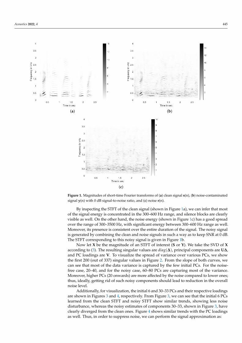
In this section, we discuss our motivation for using the PCA method for noise suppression.The idea becomes very intuitive if we can visualize the learned principal components, thesingular values, and their respective PC loadings. Thus, to do this, let s(n) be a single-channelclean time-domain speech signal, y(n) be the noise-contaminated signal with a specific signal-to-noise ratio, and r(n) be the corresponding noisy signal. Further assume that S(k,m), Y(k,m), andR(k,m) are their respective short-time Fourier transform (STFT) matrices with size 1025× 337.The magnitude of these STFTs are shown in Figure 1. To generate these STFTs, we usedHamming window of size 1024, signal overlap of 64 samples (to obtain a dense matrix forvisualization), and fast Fourier transform of size 2048. The sampling rate of the time-domainsignal was Fs = 8000 samples/s, leading to ∆ f ≈ 4 Hz. The signal-to-noise ratio was keptat 0 dB. The speech signal contained the voice of a male speaker saying “The birch canoe slidon the smooth planks”, acquired from the NOIZEUS corpus [21]. The noise (interference)signal used here was ‘Babble’ noise, also from the NOIZEUS corpus. We show these STFTs inFigure 1.

Acoustics 2022, 4 445

(a) (b)

(c)

Figure 1. Magnitudes of short-time Fourier transforms of (a) clean signal s(n), (b) noise-contaminatedsignal y(n) with 0 dB signal-to-noise ratio, and (c) noise r(n).

By inspecting the STFT of the clean signal (shown in Figure 1a), we can infer that mostof the signal energy is concentrated in the 300–600 Hz range, and silence blocks are clearlyvisible as well. On the other hand, the noise energy (shown in Figure 1c) has a good spreadover the range of 300–3500 Hz, with significant energy between 300–600 Hz range as well.Moreover, its presence is consistent over the entire duration of the signal. The noisy signalis generated by combining the clean and noise signals in such a way as to keep SNR at 0 dB.The STFT corresponding to this noisy signal is given in Figure 1b.

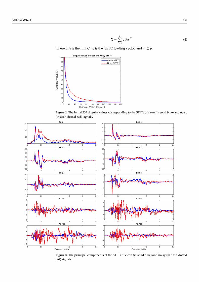
Now let X be the magnitude of an STFT of interest (S or Y). We take the SVD of Xaccording to (3). The resulting singular values are diag(∆), principal components are U∆,and PC loadings are V. To visualize the spread of variance over various PCs, we showthe first 200 (out of 337) singular values in Figure 2. From the slope of both curves, wecan see that most of the data variance is captured by the few initial PCs. For the noise-free case, 20–40, and for the noisy case, 60–80 PCs are capturing most of the variance.Moreover, higher PCs (20 onwards) are more affected by the noise compared to lower ones;thus, ideally, getting rid of such noisy components should lead to reduction in the overallnoise level.

Additionally, for visualization, the initial 6 and 30–33 PCs and their respective loadingsare shown in Figures 3 and 4, respectively. From Figure 3, we can see that the initial 6 PCslearned from the clean STFT and noisy STFT show similar trends, showing less noisedisturbance, whereas the noisy estimates of components 30–33, shown in Figure 3, haveclearly diverged from the clean ones. Figure 4 shows similar trends with the PC loadingsas well. Thus, in order to suppress noise, we can perform the signal approximation as:

Acoustics 2022, 4 446

X =q

∑i=1

uiδiv>i (4)

where uiδi is the ith PC, vi is the ith PC loading vector, and q� p.

0 20 40 60 80 100 120 140 160 180 200

Singular Value Index (i)

0

10

20

30

40

50

60

70

80

90

100S

ing

ula

r V

alu

es

iSingular Values of Clean and Noisy STFTs

Clean STFT

Noisy STFT

Figure 2. The initial 200 singular values corresponding to the STFTs of clean (in solid blue) and noisy(in dash-dotted red) signals.

0 0.5 1 1.5 2 2.5

0

20

40

60PC # 1

0 0.5 1 1.5 2 2.5

-40

-20

0

20

40

60PC # 2

0 0.5 1 1.5 2 2.5

-20

-10

0

10

20

30PC # 3

0 0.5 1 1.5 2 2.5

-20

-10

0

10

20PC # 4

0 0.5 1 1.5 2 2.5

-20

-10

0

10

20PC # 5

0 0.5 1 1.5 2 2.5

-20

-10

0

10

PC # 6

0 0.5 1 1.5 2 2.5

-4

-2

0

2

4PC # 30

0 0.5 1 1.5 2 2.5

-2

-1

0

1

2

PC # 31

0 0.5 1 1.5 2 2.5

Frequency in kHz

-2

-1

0

1

2

PC # 32

0 0.5 1 1.5 2 2.5

Frequency in kHz

-4

-2

0

2

4PC # 33

Figure 3. The principal components of the STFTs of clean (in solid blue) and noisy (in dash-dottedred) signals.

Acoustics 2022, 4 447

0.5 1 1.5 2 2.5

0.05

0.1

0.15

PC Loading # 1

0.5 1 1.5 2 2.5

-0.2

-0.1

0

0.1

PC Loading # 2

0.5 1 1.5 2 2.5

-0.1

0

0.1

0.2

0.3

PC Loading # 3

0.5 1 1.5 2 2.5

-0.2

-0.1

0

0.1

0.2

PC Loading # 4

0.5 1 1.5 2 2.5

-0.1

0

0.1

0.2

PC Loading # 5

0.5 1 1.5 2 2.5

-0.2

-0.1

0

0.1

0.2

PC Loading # 6

0.5 1 1.5 2 2.5

-0.1

0

0.1

PC Loading # 30

0.5 1 1.5 2 2.5

-0.1

0

0.1

0.2

PC Loading # 31

0.5 1 1.5 2 2.5

Time in sec

-0.2

-0.1

0

0.1

0.2

PC Loading # 32

0.5 1 1.5 2 2.5

Time in sec

-0.1

0

0.1

0.2

PC Loading # 33

Figure 4. The PC loadings of the STFTs of clean (in solid blue) and noisy (in dash-dotted red) signals.

Here, we would like to highlight two key issues with the aforementioned framework(i.e., PCA performed over the entire signal STFT). Firstly, in the signal under consideration,the noise component is present for the entire signal duration (see Figure 1c), whereas thesignal of interest, the speech signal, contains periods of silence corresponding to almost20–30% of the entire signal duration (see Figure 1a). Therefore, we can expect that thePCA computation might get biased towards learning such PCs and PC loadings, whichcan explain the entire duration of the signal. This is indeed the case, as this effect is clearlyvisible in PC 1 in Figure 3 and PC loading 1 in Figure 4. The first PC loading from the cleanSTFT (blue) clearly shows that the corresponding PC component has been able to capturethe signal variance during the time periods of voice activity. This, however, is not the casewith the first components learned from the noisy STFT, where these estimated componentshave ended up capturing a significant noise contribution as well.

Secondly, if at anytime during the signal recording, the energy of a few noisy frequen-cies gets higher than usual, then the PC and PC loading entries corresponding to thesefrequencies will become large (i.e., the corresponding singular value will get large). As aresult, these otherwise noisy components might get picked up for the STFT approximation,leading to a reduction in the effectiveness of the noise suppression.

Acoustics 2022, 4 448

In order to circumvent these issues, we propose performing noise suppression usingPCA on small subsets of STFT, instead of the complete STFT. The idea is to look at a smallnumber of time frames at a time and approximate them one by one, instead of looking atthe whole STFT. The advantage is that the SNR in each of these frames will be relativelyhigher than the SNR of the entire STFT; thus, the very few initial PCs will be able to capturemost of the data variance effectively. Additionally, the noise increase in a specific windowof time will be contained within that frame window and will not affect components in otheradjacent frames. The details of this framework are provided in the next section.

3. Block Principal Component Analysis

In this section, we formalize the block principal component analysis (termed Block-PCA) technique. Let X ∈ Rk×m be the STFT signal that we want to approximate with alow-noise version X. Here, k is the number of frequency points, and m is the number oftime frames. Let b < m be a scalar denoting the block-size, g = dm/be denote the numberof blocks, and frame-block assignment vector b = [1b, 2b, . . . , gb] ∈ Rm. Here, zb denotesa vector of size b containing z, where z ∈ Z : 1 ≤ z ≤ g. Let Xi be the matrix containingthe ith block of X, with indices coming from b. Then, we approximate Xi by first taking itsSVD, U∆V> = SVD(Xi), and doing the following:

Xi =q

∑j=1

ujδjv>j (5)

where ujδj is the jth PC, vj is the jth PC loading vector, and q� b. Thus, in this approxima-tion, we keep q most dominant components and discard the rest (b− q). We do this for alli = 1, 2, . . . , g blocks, and recreate the complete approximation matrix X =

[X1, X2, . . . , Xg

]by concatenating all block approximations.

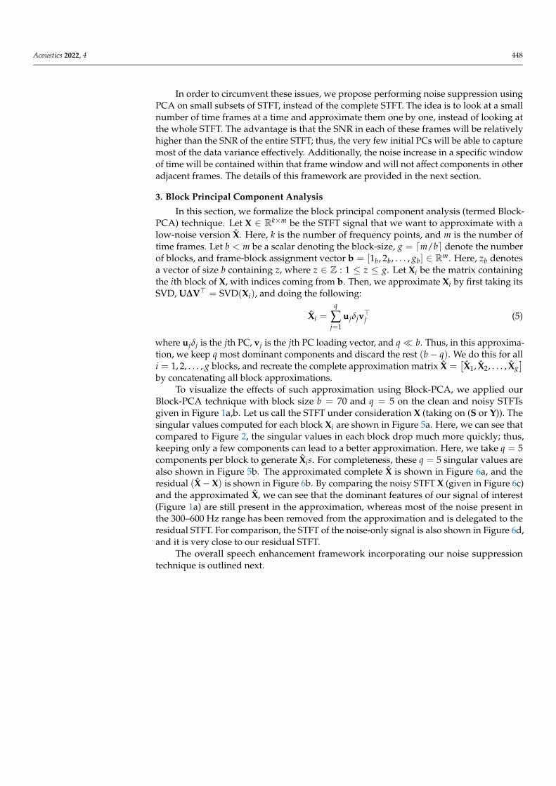
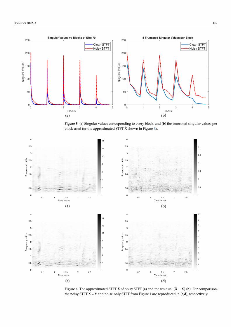
To visualize the effects of such approximation using Block-PCA, we applied ourBlock-PCA technique with block size b = 70 and q = 5 on the clean and noisy STFTsgiven in Figure 1a,b. Let us call the STFT under consideration X (taking on (S or Y)). Thesingular values computed for each block Xi are shown in Figure 5a. Here, we can see thatcompared to Figure 2, the singular values in each block drop much more quickly; thus,keeping only a few components can lead to a better approximation. Here, we take q = 5components per block to generate Xis. For completeness, these q = 5 singular values arealso shown in Figure 5b. The approximated complete X is shown in Figure 6a, and theresidual (X−X) is shown in Figure 6b. By comparing the noisy STFT X (given in Figure 6c)and the approximated X, we can see that the dominant features of our signal of interest(Figure 1a) are still present in the approximation, whereas most of the noise present inthe 300–600 Hz range has been removed from the approximation and is delegated to theresidual STFT. For comparison, the STFT of the noise-only signal is also shown in Figure 6d,and it is very close to our residual STFT.

The overall speech enhancement framework incorporating our noise suppressiontechnique is outlined next.

Acoustics 2022, 4 449

0 1 2 3 4 5

Blocks

0

50

100

150

200

250

Sin

gula

r V

alu

es

Singular Values vs Blocks of Size 70

Clean STFT

Noisy STFT

0 1 2 3 4 5

Blocks

0

50

100

150

200

250

Sin

gula

r V

alu

es

5 Truncated Singular Values per Block

Clean STFT

Noisy STFT

(a) (b)

Figure 5. (a) Singular values corresponding to every block, and (b) the truncated singular values perblock used for the approximated STFT X shown in Figure 6a.

(a) (b)

(c) (d)

Figure 6. The approximated STFT X of noisy STFT (a) and the residual (X− X) (b). For comparison,the noisy STFT X = Y and noise-only STFT from Figure 1 are reproduced in (c,d), respectively.

Acoustics 2022, 4 450

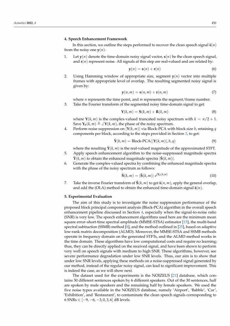
4. Speech Enhancement Framework

In this section, we outline the steps performed to recover the clean speech signal s(n)from the noisy one y(n).

1. Let y(n) denote the time-domain noisy signal vector, s(n) be the clean speech signal,and r(n) represent noise. All signals at this step are real-valued and are related by:

y(n) = s(n) + r(n) (6)

2. Using Hamming window of appropriate size, segment y(n) vector into multipleframes with appropriate level of overlap. The resulting segmented noisy signal isgiven by:

y(n, m) = s(n, m) + r(n, m) (7)

where n represents the time point, and m represents the segment/frame number.3. Take the Fourier transform of the segmented noisy time-domain signal to get:

Y(k, m) = S(k, m) + R(k, m) (8)

where Y(k, m) is the complex-valued truncated noisy spectrum with k = n/2 + 1.Save Yθ(k, m) , ∠Y(k, m), the phase of the noisy spectrum.

4. Perform noise suppression on |Y(k, m)| via Block-PCA with block size b, retaining qcomponents per block, according to the steps provided in Section 3, to get:

Y(k, m) = Block-PCA(|Y(k, m)|, b, q) (9)

where the resulting Y(k, m) is the real-valued magnitude of the approximated STFT.5. Apply speech enhancement algorithm to the noise-suppressed magnitude spectra

Y(k, m) to obtain the enhanced magnitude spectra |S(k, m)|.6. Generate the complex-valued spectra by combining the enhanced magnitude spectra

with the phase of the noisy spectrum as follows:

S(k, m) = |S(k, m)| ejYθ(k,m) (10)

7. Take the inverse Fourier transform of S(k, m) to get s(n, m), apply the general overlap,and add the (OLA) method to obtain the enhanced time-domain signal s(n).

5. Experimental Evaluation

The aim of this study is to investigate the noise suppression performance of theproposed block principal component analysis (Block-PCA) algorithm in the overall speechenhancement pipeline discussed in Section 4, especially when the signal-to-noise ratio(SNR) is very low. The speech enhancement algorithms used here are the minimum meansquare error–short-time spectral amplitude (MMSE-STSA) estimator [15], the multi-bandspectral subtraction (SSMB) method [8], and the method outlined in [25], based on adaptivelow-rank matrix decomposition (ALMD). Moreover, the MMSE-STSA and SSMB methodsoperate in frequency domain on the generated STFTs, and the ALMD method works inthe time domain. These algorithms have low computational costs and require no learning;thus, they can be directly applied on the received signal, and have been shown to performvery well on speech signals with medium to high SNR. These algorithms, however, seesevere performance degradation under low SNR levels. Thus, our aim is to show thatunder low SNR levels, applying these methods on a noise-suppressed signal generated byour method, instead of the regular noisy signal, can lead to significant improvement. Thisis indeed the case, as we will show next.

The dataset used for the experiments is the NOIZEUS [21] database, which con-tains 30 different sentences spoken by 6 different speakers. Out of the 30 sentences, halfare spoken by male speakers and the remaining half by female speakers. We used thefive noise types available in the NOIZEUS database, namely ‘Airport’, ‘Babble’, ‘Car’,‘Exhibition’, and ‘Restaurant’, to contaminate the clean speech signals corresponding to6 SNRs ∈ [−9,−6,−3, 0, 3, 6] dB levels.

Acoustics 2022, 4 451

The metrics used to evaluate the enhanced speech quality are segmental SNR(SSNR) [39] and the perceptual evaluation of speech quality (PESQ) [40]. In addition, wehave used the composite measures Csig, Cbak, and Covl [40] to rate the speech distortion,noise distortion, and the overall quality, respectively, of the enhanced speech signal.These composite measures are the linear combinations of PESQ, log likelihood ratio(LLR) [41], and weighted-slope spectral (WSS) distance [42] scores.

In all the experiments discussed next, the sampling rate of the speech signals wasfixed at Fs = 8000 Hz, and we used Hamming window of size 200 samples (25 msduration), with overlap of 80 samples (10 ms) to compute the short-time Fourier transformof the signal under analysis. The FFT size was set equal to the chosen window size. Lets(n) be the clean speech signal, and r(n) be the noise signal of a specific type. Wegenerate the noise-contaminated signal y(n) with a specific SNR level by adding r(n)with specific energy to s(n). We perform speech enhancement using the frameworkoutlined in Section 4 with and without performing noise suppression via Block-PCA toanalyze its effectiveness. As the ALMD algorithm operates in the time domain, afterperforming STFT approximation of the noisy signal using Block-PCA, we recreate thenoise-suppressed time-domain signal using inverse Fourier transform and the overlapand add method. This signal is then passed to the ALMD algorithm for enhancement. Westore the performance scores for the noisy input signal, MMSE-STSA only, MMSE-STSAwith Block-PCA, SSMB only, SSMB with Block-PCA, ALMD only, and ALMD with Block-PCA. We repeat this process for all 30 speech signals, all 6 SNR levels, and for all noisetypes, as discussed earlier. The block size (b) and components to retain (q) are selected byperforming a 2-D grid search over b = [40, 50, 60, 70] and q = [15, 16, . . . , 26] and choosingthe combination that leads to highest performance. These results are presented andanalyzed next.

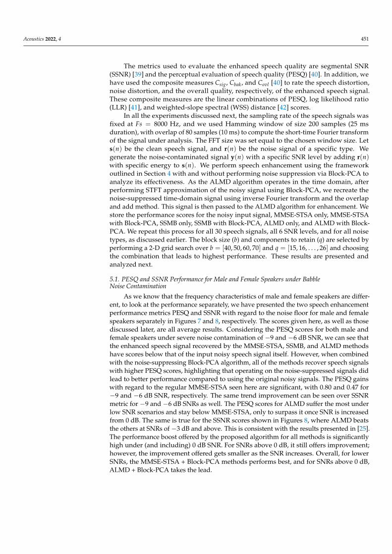
5.1. PESQ and SSNR Performance for Male and Female Speakers under BabbleNoise Contamination

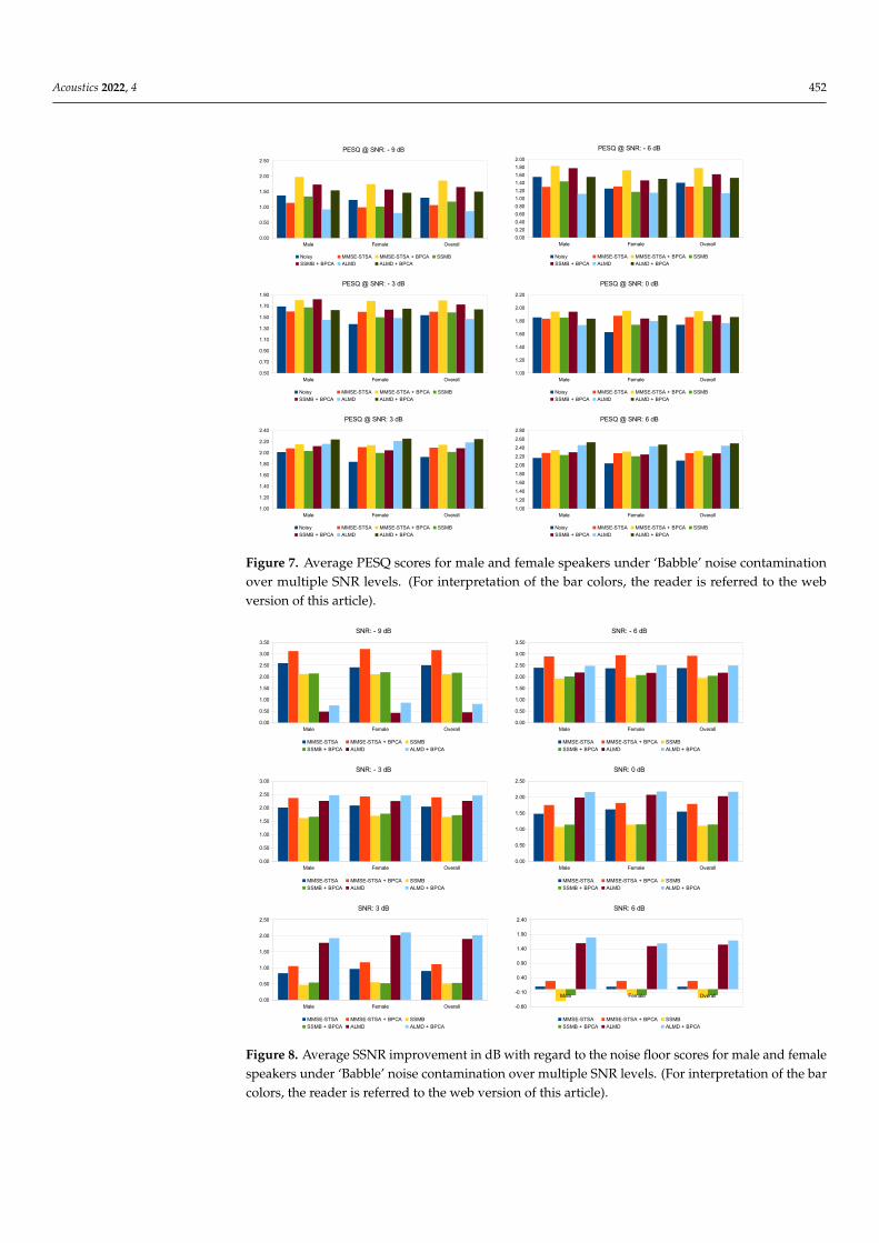
As we know that the frequency characteristics of male and female speakers are differ-ent, to look at the performance separately, we have presented the two speech enhancementperformance metrics PESQ and SSNR with regard to the noise floor for male and femalespeakers separately in Figures 7 and 8, respectively. The scores given here, as well as thosediscussed later, are all average results. Considering the PESQ scores for both male andfemale speakers under severe noise contamination of −9 and −6 dB SNR, we can see thatthe enhanced speech signal recovered by the MMSE-STSA, SSMB, and ALMD methodshave scores below that of the input noisy speech signal itself. However, when combinedwith the noise-suppressing Block-PCA algorithm, all of the methods recover speech signalswith higher PESQ scores, highlighting that operating on the noise-suppressed signals didlead to better performance compared to using the original noisy signals. The PESQ gainswith regard to the regular MMSE-STSA seen here are significant, with 0.80 and 0.47 for−9 and −6 dB SNR, respectively. The same trend improvement can be seen over SSNRmetric for −9 and −6 dB SNRs as well. The PESQ scores for ALMD suffer the most underlow SNR scenarios and stay below MMSE-STSA, only to surpass it once SNR is increasedfrom 0 dB. The same is true for the SSNR scores shown in Figures 8, where ALMD beatsthe others at SNRs of −3 dB and above. This is consistent with the results presented in [25].The performance boost offered by the proposed algorithm for all methods is significantlyhigh under (and including) 0 dB SNR. For SNRs above 0 dB, it still offers improvement;however, the improvement offered gets smaller as the SNR increases. Overall, for lowerSNRs, the MMSE-STSA + Block-PCA methods performs best, and for SNRs above 0 dB,ALMD + Block-PCA takes the lead.

Acoustics 2022, 4 452

Figure 7. Average PESQ scores for male and female speakers under ‘Babble’ noise contaminationover multiple SNR levels. (For interpretation of the bar colors, the reader is referred to the webversion of this article).

Figure 8. Average SSNR improvement in dB with regard to the noise floor scores for male and femalespeakers under ‘Babble’ noise contamination over multiple SNR levels. (For interpretation of the barcolors, the reader is referred to the web version of this article).

Acoustics 2022, 4 453

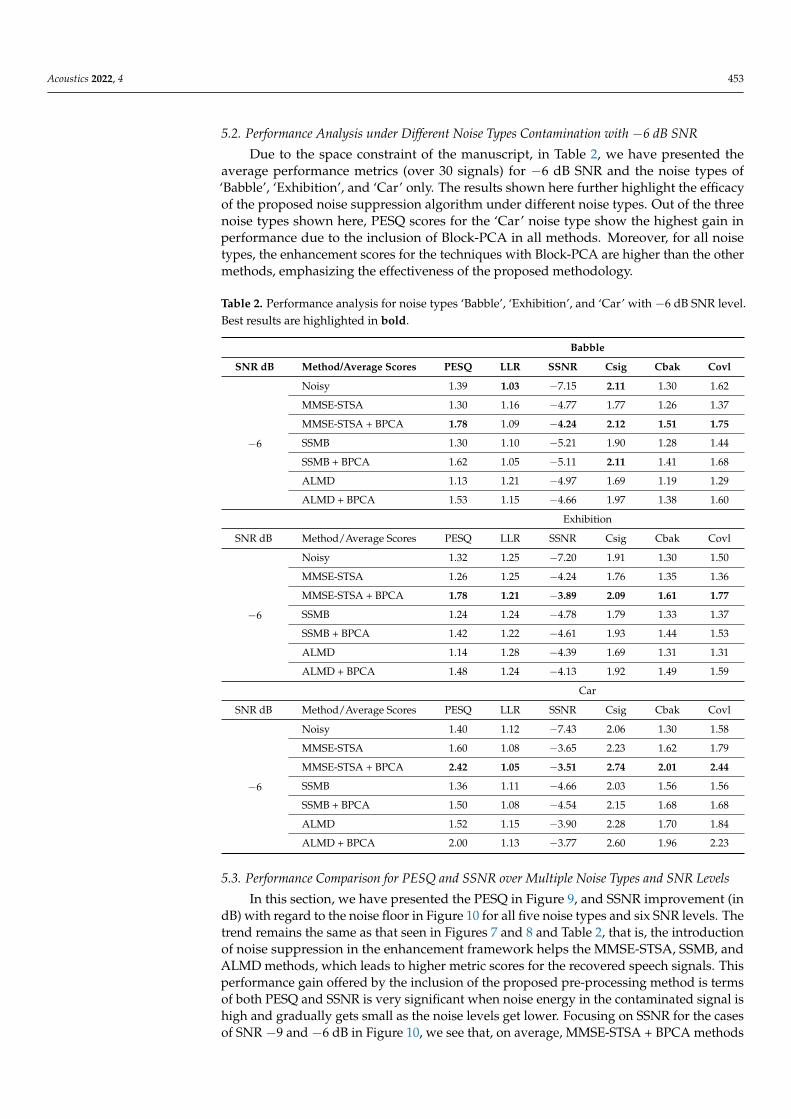
5.2. Performance Analysis under Different Noise Types Contamination with −6 dB SNR

Due to the space constraint of the manuscript, in Table 2, we have presented theaverage performance metrics (over 30 signals) for −6 dB SNR and the noise types of‘Babble’, ‘Exhibition’, and ‘Car’ only. The results shown here further highlight the efficacyof the proposed noise suppression algorithm under different noise types. Out of the threenoise types shown here, PESQ scores for the ‘Car’ noise type show the highest gain inperformance due to the inclusion of Block-PCA in all methods. Moreover, for all noisetypes, the enhancement scores for the techniques with Block-PCA are higher than the othermethods, emphasizing the effectiveness of the proposed methodology.

Table 2. Performance analysis for noise types ‘Babble’, ‘Exhibition’, and ‘Car’ with −6 dB SNR level.Best results are highlighted in bold.

Babble

SNR dB Method/Average Scores PESQ LLR SSNR Csig Cbak Covl

−6

Noisy 1.39 1.03 −7.15 2.11 1.30 1.62

MMSE-STSA 1.30 1.16 −4.77 1.77 1.26 1.37

MMSE-STSA + BPCA 1.78 1.09 −4.24 2.12 1.51 1.75

SSMB 1.30 1.10 −5.21 1.90 1.28 1.44

SSMB + BPCA 1.62 1.05 −5.11 2.11 1.41 1.68

ALMD 1.13 1.21 −4.97 1.69 1.19 1.29

ALMD + BPCA 1.53 1.15 −4.66 1.97 1.38 1.60

Exhibition

SNR dB Method/Average Scores PESQ LLR SSNR Csig Cbak Covl

−6

Noisy 1.32 1.25 −7.20 1.91 1.30 1.50

MMSE-STSA 1.26 1.25 −4.24 1.76 1.35 1.36

MMSE-STSA + BPCA 1.78 1.21 −3.89 2.09 1.61 1.77

SSMB 1.24 1.24 −4.78 1.79 1.33 1.37

SSMB + BPCA 1.42 1.22 −4.61 1.93 1.44 1.53

ALMD 1.14 1.28 −4.39 1.69 1.31 1.31

ALMD + BPCA 1.48 1.24 −4.13 1.92 1.49 1.59

Car

SNR dB Method/Average Scores PESQ LLR SSNR Csig Cbak Covl

−6

Noisy 1.40 1.12 −7.43 2.06 1.30 1.58

MMSE-STSA 1.60 1.08 −3.65 2.23 1.62 1.79

MMSE-STSA + BPCA 2.42 1.05 −3.51 2.74 2.01 2.44

SSMB 1.36 1.11 −4.66 2.03 1.56 1.56

SSMB + BPCA 1.50 1.08 −4.54 2.15 1.68 1.68

ALMD 1.52 1.15 −3.90 2.28 1.70 1.84

ALMD + BPCA 2.00 1.13 −3.77 2.60 1.96 2.23

5.3. Performance Comparison for PESQ and SSNR over Multiple Noise Types and SNR Levels

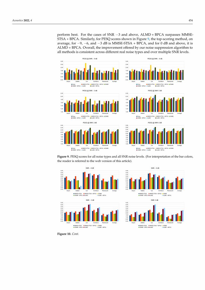
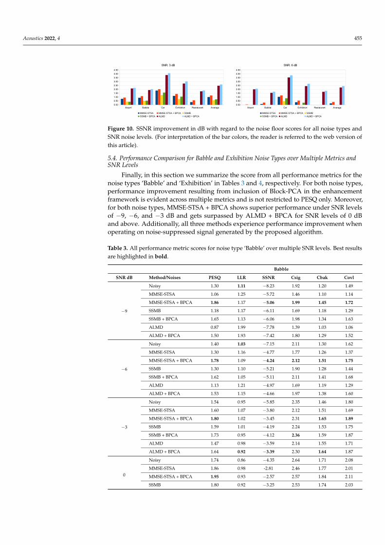
In this section, we have presented the PESQ in Figure 9, and SSNR improvement (indB) with regard to the noise floor in Figure 10 for all five noise types and six SNR levels. Thetrend remains the same as that seen in Figures 7 and 8 and Table 2, that is, the introductionof noise suppression in the enhancement framework helps the MMSE-STSA, SSMB, andALMD methods, which leads to higher metric scores for the recovered speech signals. Thisperformance gain offered by the inclusion of the proposed pre-processing method is termsof both PESQ and SSNR is very significant when noise energy in the contaminated signal ishigh and gradually gets small as the noise levels get lower. Focusing on SSNR for the casesof SNR −9 and −6 dB in Figure 10, we see that, on average, MMSE-STSA + BPCA methods

Acoustics 2022, 4 454

perform best. For the cases of SNR −3 and above, ALMD + BPCA surpasses MMSE-STSA + BPCA. Similarly, for PESQ scores shown in Figure 9, the top-scoring method, onaverage, for −9, −6, and −3 dB is MMSE-STSA + BPCA, and for 0 dB and above, it isALMD + BPCA. Overall, the improvement offered by our noise suppression algorithm toall methods is consistent across different real noise types and over multiple SNR levels.

Figure 9. PESQ scores for all noise types and all SNR noise levels. (For interpretation of the bar colors,the reader is referred to the web version of this article).

Figure 10. Cont.

Acoustics 2022, 4 455

Figure 10. SSNR improvement in dB with regard to the noise floor scores for all noise types andSNR noise levels. (For interpretation of the bar colors, the reader is referred to the web version ofthis article).

5.4. Performance Comparison for Babble and Exhibition Noise Types over Multiple Metrics andSNR Levels

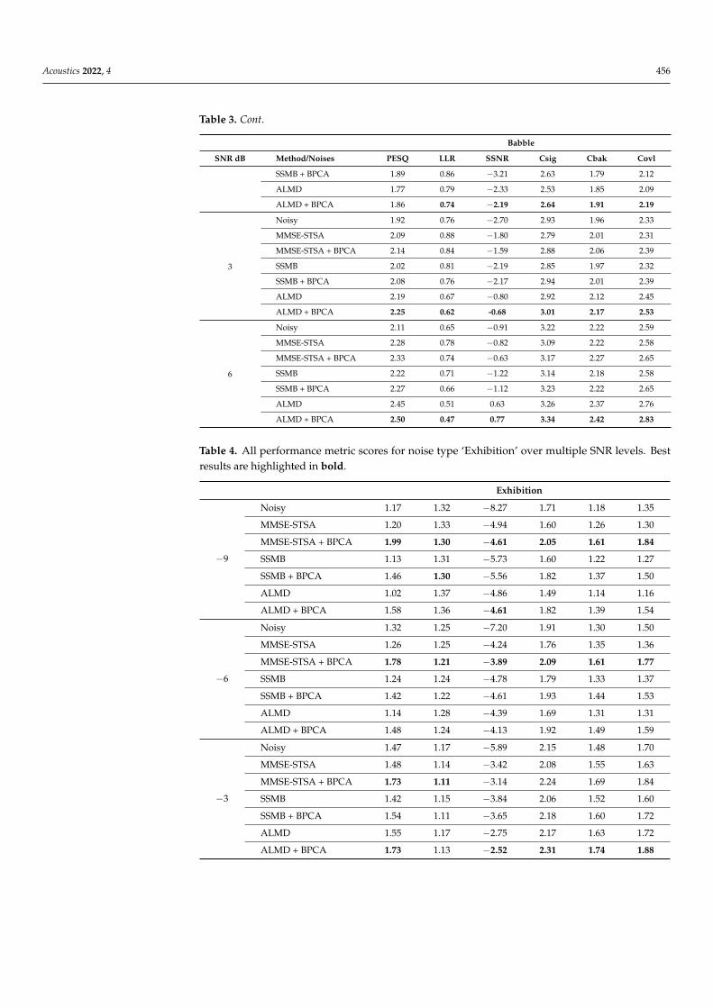
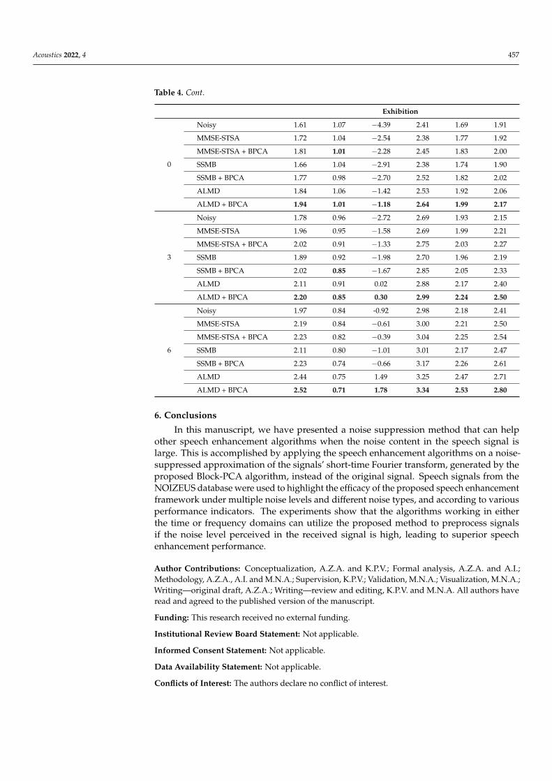
Finally, in this section we summarize the score from all performance metrics for thenoise types ‘Babble’ and ‘Exhibition’ in Tables 3 and 4, respectively. For both noise types,performance improvement resulting from inclusion of Block-PCA in the enhancementframework is evident across multiple metrics and is not restricted to PESQ only. Moreover,for both noise types, MMSE-STSA + BPCA shows superior performance under SNR levelsof −9, −6, and −3 dB and gets surpassed by ALMD + BPCA for SNR levels of 0 dBand above. Additionally, all three methods experience performance improvement whenoperating on noise-suppressed signal generated by the proposed algorithm.

Table 3. All performance metric scores for noise type ‘Babble’ over multiple SNR levels. Best resultsare highlighted in bold.

Babble

SNR dB Method/Noises PESQ LLR SSNR Csig Cbak Covl

−9

Noisy 1.30 1.11 −8.23 1.92 1.20 1.49

MMSE-STSA 1.06 1.25 −5.72 1.46 1.10 1.14

MMSE-STSA + BPCA 1.86 1.17 −5.06 1.99 1.45 1.72

SSMB 1.18 1.17 −6.11 1.69 1.18 1.29

SSMB + BPCA 1.65 1.13 −6.06 1.98 1.34 1.63

ALMD 0.87 1.99 −7.78 1.39 1.03 1.06

ALMD + BPCA 1.50 1.93 −7.42 1.80 1.29 1.52

−6

Noisy 1.40 1.03 −7.15 2.11 1.30 1.62

MMSE-STSA 1.30 1.16 −4.77 1.77 1.26 1.37

MMSE-STSA + BPCA 1.78 1.09 −4.24 2.12 1.51 1.75

SSMB 1.30 1.10 −5.21 1.90 1.28 1.44

SSMB + BPCA 1.62 1.05 −5.11 2.11 1.41 1.68

ALMD 1.13 1.21 −4.97 1.69 1.19 1.29

ALMD + BPCA 1.53 1.15 −4.66 1.97 1.38 1.60

−3

Noisy 1.54 0.95 −5.85 2.35 1.46 1.80

MMSE-STSA 1.60 1.07 −3.80 2.12 1.51 1.69

MMSE-STSA + BPCA 1.80 1.02 −3.45 2.31 1.65 1.89

SSMB 1.59 1.01 −4.19 2.24 1.53 1.75

SSMB + BPCA 1.73 0.95 −4.12 2.36 1.59 1.87

ALMD 1.47 0.98 −3.59 2.14 1.55 1.71

ALMD + BPCA 1.64 0.92 −3.39 2.30 1.64 1.87

0

Noisy 1.74 0.86 −4.35 2.64 1.71 2.08

MMSE-STSA 1.86 0.98 -2.81 2.46 1.77 2.01

MMSE-STSA + BPCA 1.95 0.93 −2.57 2.57 1.84 2.11

SSMB 1.80 0.92 −3.25 2.53 1.74 2.03

Acoustics 2022, 4 456

Table 3. Cont.

Babble

SNR dB Method/Noises PESQ LLR SSNR Csig Cbak Covl

SSMB + BPCA 1.89 0.86 −3.21 2.63 1.79 2.12

ALMD 1.77 0.79 −2.33 2.53 1.85 2.09

ALMD + BPCA 1.86 0.74 −2.19 2.64 1.91 2.19

3

Noisy 1.92 0.76 −2.70 2.93 1.96 2.33

MMSE-STSA 2.09 0.88 −1.80 2.79 2.01 2.31

MMSE-STSA + BPCA 2.14 0.84 −1.59 2.88 2.06 2.39

SSMB 2.02 0.81 −2.19 2.85 1.97 2.32

SSMB + BPCA 2.08 0.76 −2.17 2.94 2.01 2.39

ALMD 2.19 0.67 −0.80 2.92 2.12 2.45

ALMD + BPCA 2.25 0.62 -0.68 3.01 2.17 2.53

6

Noisy 2.11 0.65 −0.91 3.22 2.22 2.59

MMSE-STSA 2.28 0.78 −0.82 3.09 2.22 2.58

MMSE-STSA + BPCA 2.33 0.74 −0.63 3.17 2.27 2.65

SSMB 2.22 0.71 −1.22 3.14 2.18 2.58

SSMB + BPCA 2.27 0.66 −1.12 3.23 2.22 2.65

ALMD 2.45 0.51 0.63 3.26 2.37 2.76

ALMD + BPCA 2.50 0.47 0.77 3.34 2.42 2.83

Table 4. All performance metric scores for noise type ‘Exhibition’ over multiple SNR levels. Bestresults are highlighted in bold.

Exhibition

−9

Noisy 1.17 1.32 −8.27 1.71 1.18 1.35

MMSE-STSA 1.20 1.33 −4.94 1.60 1.26 1.30

MMSE-STSA + BPCA 1.99 1.30 −4.61 2.05 1.61 1.84

SSMB 1.13 1.31 −5.73 1.60 1.22 1.27

SSMB + BPCA 1.46 1.30 −5.56 1.82 1.37 1.50

ALMD 1.02 1.37 −4.86 1.49 1.14 1.16

ALMD + BPCA 1.58 1.36 −4.61 1.82 1.39 1.54

−6

Noisy 1.32 1.25 −7.20 1.91 1.30 1.50

MMSE-STSA 1.26 1.25 −4.24 1.76 1.35 1.36

MMSE-STSA + BPCA 1.78 1.21 −3.89 2.09 1.61 1.77

SSMB 1.24 1.24 −4.78 1.79 1.33 1.37

SSMB + BPCA 1.42 1.22 −4.61 1.93 1.44 1.53

ALMD 1.14 1.28 −4.39 1.69 1.31 1.31

ALMD + BPCA 1.48 1.24 −4.13 1.92 1.49 1.59

−3

Noisy 1.47 1.17 −5.89 2.15 1.48 1.70

MMSE-STSA 1.48 1.14 −3.42 2.08 1.55 1.63

MMSE-STSA + BPCA 1.73 1.11 −3.14 2.24 1.69 1.84

SSMB 1.42 1.15 −3.84 2.06 1.52 1.60

SSMB + BPCA 1.54 1.11 −3.65 2.18 1.60 1.72

ALMD 1.55 1.17 −2.75 2.17 1.63 1.72

ALMD + BPCA 1.73 1.13 −2.52 2.31 1.74 1.88

Acoustics 2022, 4 457

Table 4. Cont.

Exhibition

0

Noisy 1.61 1.07 −4.39 2.41 1.69 1.91

MMSE-STSA 1.72 1.04 −2.54 2.38 1.77 1.92

MMSE-STSA + BPCA 1.81 1.01 −2.28 2.45 1.83 2.00

SSMB 1.66 1.04 −2.91 2.38 1.74 1.90

SSMB + BPCA 1.77 0.98 −2.70 2.52 1.82 2.02

ALMD 1.84 1.06 −1.42 2.53 1.92 2.06

ALMD + BPCA 1.94 1.01 −1.18 2.64 1.99 2.17

3

Noisy 1.78 0.96 −2.72 2.69 1.93 2.15

MMSE-STSA 1.96 0.95 −1.58 2.69 1.99 2.21

MMSE-STSA + BPCA 2.02 0.91 −1.33 2.75 2.03 2.27

SSMB 1.89 0.92 −1.98 2.70 1.96 2.19

SSMB + BPCA 2.02 0.85 −1.67 2.85 2.05 2.33

ALMD 2.11 0.91 0.02 2.88 2.17 2.40

ALMD + BPCA 2.20 0.85 0.30 2.99 2.24 2.50

6

Noisy 1.97 0.84 -0.92 2.98 2.18 2.41

MMSE-STSA 2.19 0.84 −0.61 3.00 2.21 2.50

MMSE-STSA + BPCA 2.23 0.82 −0.39 3.04 2.25 2.54

SSMB 2.11 0.80 −1.01 3.01 2.17 2.47

SSMB + BPCA 2.23 0.74 −0.66 3.17 2.26 2.61

ALMD 2.44 0.75 1.49 3.25 2.47 2.71

ALMD + BPCA 2.52 0.71 1.78 3.34 2.53 2.80

6. Conclusions

In this manuscript, we have presented a noise suppression method that can helpother speech enhancement algorithms when the noise content in the speech signal islarge. This is accomplished by applying the speech enhancement algorithms on a noise-suppressed approximation of the signals’ short-time Fourier transform, generated by theproposed Block-PCA algorithm, instead of the original signal. Speech signals from theNOIZEUS database were used to highlight the efficacy of the proposed speech enhancementframework under multiple noise levels and different noise types, and according to variousperformance indicators. The experiments show that the algorithms working in eitherthe time or frequency domains can utilize the proposed method to preprocess signalsif the noise level perceived in the received signal is high, leading to superior speechenhancement performance.

Author Contributions: Conceptualization, A.Z.A. and K.P.V.; Formal analysis, A.Z.A. and A.I.;Methodology, A.Z.A., A.I. and M.N.A.; Supervision, K.P.V.; Validation, M.N.A.; Visualization, M.N.A.;Writing—original draft, A.Z.A.; Writing—review and editing, K.P.V. and M.N.A. All authors haveread and agreed to the published version of the manuscript.

Funding: This research received no external funding.

Institutional Review Board Statement: Not applicable.

Informed Consent Statement: Not applicable.

Data Availability Statement: Not applicable.

Conflicts of Interest: The authors declare no conflict of interest.

Acoustics 2022, 4 458

References1. Loizou, P.C. Speech Enhancement: Theory and Practice; CRC Press: Boca Raton, FL, USA, 2013.2. Veisi, H.; Sameti, H. Hidden-Markov-model-based voice activity detector with high speech detection rate for speech enhancement.

IET Signal Process. 2012, 6, 54–63. [CrossRef]3. Wei, H.; Long, Y.; Mao, H. Improvements on self-adaptive voice activity detector for telephone data. Int. J. Speech Technol. 2016,

19, 623–630. [CrossRef]4. Sayoud, A.; Djendi, M. Efficient subband fast adaptive algorithm based-backward blind source separation for speech intelligibility

enhancement. Int. J. Speech Technol. 2020, 23, 471–479. [CrossRef]5. Bahadur, I.N.; Kumar, S.; Agarwal, P. Performance measurement of a hybrid speech enhancement technique. Int. J. Speech Technol.

2021, 24, 665–677. [CrossRef]6. Sanam, T.F.; Shahnaz, C. A semisoft thresholding method based on Teager energy operation on wavelet packet coefficients for

enhancing noisy speech. EURASIP J. Audio Speech Music. Process. 2013, 2013, 25. [CrossRef]7. Boll, S. Suppression of acoustic noise in speech using spectral subtraction. IEEE Trans. Acoust. Speech Signal Process. 1979,

27, 113–120. [CrossRef]8. Kamath, S.; Loizou, P. A multi-band spectral subtraction method for enhancing speech corrupted by colored noise. In Proceedings

of the 2002 IEEE International Conference on Acoustics, Speech, and Signal Processing, Orlando, FL, USA, 13–17 May 2002;Volume 4, p. 44164.

9. Yadava, T.G.; Jayanna, H.S. Speech enhancement by combining spectral subtraction and minimum mean square error-spectrumpower estimator based on zero crossing. Int. J. Speech Technol. 2019, 22, 639–648. [CrossRef]

10. Nahma, L.; Yong, P.C.; Dam, H.H.; Nordholm, S. An adaptive a priori SNR estimator for perceptual speech enhancement. EurasipJ. Audio Speech Music Process. 2019, 2019, 7. [CrossRef]

11. Farahani, G. Autocorrelation-based noise subtraction method with smoothing, overestimation, energy, and cepstral mean andvariance normalization for noisy speech recognition. EURASIP J. Audio Speech Music. Process. 2017, 2017, 13. [CrossRef]

12. Abd El-Fattah, M.A.; Dessouky, M.I.; Abbas, A.M.; Diab, S.M.; El-Rabaie, E.S.M.; Al-Nuaimy, W.; Alshebeili, S.A.; Abd El-Samie,F.E. Speech enhancement with an adaptive Wiener filter. Int. J. Speech Technol. 2014, 17, 53–64. [CrossRef]

13. Catic, J.; Dau, T.; Buchholz, J.; Gran, F. The Effect of a Voice Activity Detector on the Speech Enhancement Performance of theBinaural Multichannel Wiener Filter. EURASIP J. Audio Speech Music Process. 2010, 2010, 840294. [CrossRef]

14. Ma, Y.; Nishihara, A. A modified Wiener filtering method combined with wavelet thresholding multitaper spectrum for speechenhancement. EURASIP J. Audio Speech Music Process. 2014, 2014, 32. [CrossRef]

15. Ephraim, Y.; Malah, D. Speech enhancement using a minimum-mean square error short-time spectral amplitude estimator. IEEETrans. Acoust. Speech Signal Process. 1984, 32, 1109–1121. [CrossRef]

16. Ephraim, Y.; Malah, D. Speech enhancement using a minimum mean-square error log-spectral amplitude estimator. IEEE Trans.Acoust. Speech Signal Process. 1985, 33, 443–445. [CrossRef]

17. You, C.H.; Koh, S.N.; Rahardja, S. /spl beta/-order MMSE spectral amplitude estimation for speech enhancement. IEEE Trans.Speech Audio Process. 2005, 13, 475–486.

18. Bahrami, M.; Faraji, N. Minimum mean square error estimator for speech enhancement in additive noise assuming Weibullspeech priors and speech presence uncertainty. Int. J. Speech Technol. 2021, 24, 97–108. [CrossRef]

19. Sayoud, A.; Djendi, M.; Guessoum, A. A new speech enhancement adaptive algorithm based on fullband–subband MSEswitching. Int. J. Speech Technol. 2019, 22, 993–1005. [CrossRef]

20. Roy, S.K.; Paliwal, K.K. A noise PSD estimation algorithm using derivative-based high-pass filter in non-stationary noiseconditions. EURASIP J. Audio Speech Music Process. 2021, 2021, 32. [CrossRef]

21. Hu, Y. Subjective evaluation and comparison of speech enhancement algorithms. Speech Commun. 2007, 49, 588–601. [CrossRef]22. Kumar, B. Comparative performance evaluation of MMSE-based speech enhancement techniques through simulation and

real-time implementation. Int. J. Speech Technol. 2018, 21, 1033–1044. [CrossRef]23. Ji, Y.; Zhu, W.P.; Champagne, B. Speech Enhancement Based on Dictionary Learning and Low-Rank Matrix Decomposition. IEEE

Access 2018, 7, 4936–4947. [CrossRef]24. Sigg, C.D.; Dikk, T.; Buhmann, J.M. Speech enhancement using generative dictionary learning. IEEE Trans. Audio Speech Lang.

Process. 2012, 20, 1698–1712. [CrossRef]25. Li, C.; Jiang, T.; Wu, S.; Xie, J. Single-Channel Speech Enhancement Based on Adaptive Low-Rank Matrix Decomposition. IEEE

Access 2020, 8, 37066–37076. [CrossRef]26. Jolliffe, I.T.; Cadima, J. Principal component analysis: A review and recent developments. Philos. Trans. R. Soc. Math. Phys. Eng.

Sci. 2016, 374, 20150202. [CrossRef]27. Koch, I. Analysis of Multivariate and High-Dimensional Data; Cambridge University Press: Cambridge, UK, 2013; Volume 32.28. Pyatykh, S.; Hesser, J.; Zheng, L. Image noise level estimation by principal component analysis. IEEE Trans. Image Process. 2012,

22, 687–699. [CrossRef]29. Zhang, L.; Lukac, R.; Wu, X.; Zhang, D. PCA-based spatially adaptive denoising of CFA images for single-sensor digital cameras.

IEEE Trans. Image Process. 2009, 18, 797–812. [CrossRef]30. Srinivasarao, V.; Ghanekar, U. Speech enhancement—An enhanced principal component analysis (EPCA) filter approach. Comput.

Electr. Eng. 2020, 85, 106657. [CrossRef]

Acoustics 2022, 4 459

31. Sun, P.; Qin, J. Low-rank and sparsity analysis applied to speech enhancement via online estimated dictionary. IEEE SignalProcess. Lett. 2016, 23, 1862–1866. [CrossRef]

32. Khalilian, H.; Bajic, I.V. Video watermarking with empirical PCA-based decoding. IEEE Trans. Image Process. 2013, 22, 4825–4840.[CrossRef]

33. Vaswani, N.; Chellappa, R. Principal components null space analysis for image and video classification. IEEE Trans. Image Process.2006, 15, 1816–1830. [CrossRef]

34. Seghouane, A.K.; Iqbal, A.; Desai, N.K. BSmCCA: A block sparse multiple-set canonical correlation analysis algorithm formulti-subject fMRI data sets. In Proceedings of the 2017 IEEE International Conference on Acoustics, Speech and Signal Processing(ICASSP), New Orleans, LA, USA, 5–9 March 2017; pp. 6324–6328.

35. Seghouane, A.K.; Iqbal, A. The Adaptive Block Sparse PCA and its Application to Multi-Subject fMRI Data Analysis Using SparsemCCA. Signal Process. 2018, 153, 311–320. [CrossRef]

36. Caruso, G.; Battista, T.D.; Gattone, S.A. A micro-level analysis of regional economic activity through a PCA approach. InProceedings of the International Conference on Decision Economics, Ávila, Spain, 26–28 June 2019; pp. 227–234.

37. Yang, J.; Zhang, D.; Frangi, A.F.; Yang, J.Y. Two-dimensional PCA: A new approach to appearance-based face representation andrecognition. IEEE Trans. Pattern Anal. Mach. Intell. 2004, 26, 131–137. [CrossRef] [PubMed]

38. Bishop, C.M. Pattern Recognition and Machine Learning; Springer: New York, NY, USA, 2006.39. Du, J.; Huo, Q. A speech enhancement approach using piecewise linear approximation of an explicit model of environmen-

tal distortions. In Proceedings of the Ninth Annual Conference of the International Speech Communication Association,Brisbane, QLD, Australia, 22–26 September 2008.

40. Hu, Y.; Loizou, P.C. Evaluation of objective quality measures for speech enhancement. IEEE Trans. Audio Speech Lang. Process.2007, 16, 229–238. [CrossRef]

41. Quackenbush, S.R. Objective Measures of Speech Quality (Subjective). Ph.D. Dissertation, The University of Michigan, AnnArbor, MI, USA, 1986.

42. Klatt, D. Prediction of perceived phonetic distance from critical-band spectra: A first step. In Proceedings of the ICASSP’82 IEEEInternational Conference on Acoustics, Speech, and Signal Processing, Paris, France, 3–5 May 1982; Volume 7, pp. 1278–1281.