Lifetime of Metastable States and Suppression of Noise in Interdisciplinary Physical Models

arX

iv:0

810.

0712

v1 [

cond

-mat

.sta

t-m

ech]

4 O

ct 2

008

Lifetime of metastable states and suppression of noise inInterdisciplinary Physical Models ∗

B. Spagnoloa†, A. A. Dubkovb, A. L. Pankratovc,

E. V. Pankratovad, A. Fiasconaroa,e,f , A. Ochab-Marcineke

aDipartimento di Fisica e Tecnologie Relative, Universita di PalermoCNISM - Unita di Palermo, Group of Interdisciplinary Physics‡

Viale delle Scienze, I-90128 Palermo, ItalybRadiophysics Department, Nizhny Novgorod State University, 23 Gagarin ave.,

603950 Nizhny Novgorod, RussiacInstitute for Physics of Microstructures of RAS, GSP-105, Nizhny Novgorod,

603950, RussiadMathematical Department, Volga State Academy, Nesterov street 5,

Nizhny Novgorod, 603600, RussiaeMarian Smoluchowski Institute of Physics, Jagellonian University

Reymonta 4, 30059 Krakw, PolandfMark Kac Center for Complex Systems Research, Jagellonian University

Reymonta 4, 30059 Krakw, Poland

Transient properties of different physical systems with metastable statesperturbed by external white noise have been investigated. Two noise-induced phenomena, namely the noise enhanced stability and the reso-nant activation, are theoretically predicted in a piece-wise linear fluctuat-ing potential with a metastable state. The enhancement of the lifetime ofmetastable states due to the noise, and the suppression of noise throughresonant activation phenomenon will be reviewed in models of interdisci-plinary physics: (i) dynamics of an overdamped Josephson junction; (ii)transient regime of the noisy FitzHugh-Nagumo model; (iii) populationdynamics.

PACS numbers: 05.10.-a, 05.40.-a, 87.23.Cc

∗ Presented at the 19th Marian Smoluchowski Symposium on Statistical Physics,Krakow, Poland, May 14-17, 2006

† e-mail: [email protected]‡ http://gip.dft.unipa.it

(1)

http://arXiv.org/abs/0810.0712v1

2 spagnolo˙20.04.07 printed on October 4, 2008

1. Introduction

Metastability is a generic feature of many nonlinear systems, and theproblem of the lifetime of metastable states involves fundamental aspects ofnonequilibrium statistical mechanics. Nonequilibrium systems are usuallyopen systems which strongly interact with environment through exchang-ing materials and energy, which can be modelled as noise. The investigationof noise-induced phenomena in far from equilibrium systems is one of theapproaches used to understand the behaviour of physical and biological com-plex systems. Specifically the relaxation in many natural complex systemsproceeds through metastable states and this transient behaviour is observedin condensed matter physics and in different other fields, such as cosmol-ogy, chemical kinetics, biology and high energy physics [1]-[9]. In spite ofsuch ubiquity, the microscopic understanding of metastability still raisesfundamental questions, such as those related to the fluctuation-dissipationtheorem in transient dynamics [10].

Recently, the investigation of the thermal acivated escape in systemswith fluctuating metastable states has led to the discovery of resonancelikephenomena, characterized by a nonmonotonic behavior of the lifetime ofthe metastable state as a function of the noise intensity or the driving fre-quency. Among these we recall two of them, namely the resonant activation(RA) phenomenon [11]-[21], whose signature is a minimum of the lifetimeof the metastable state as a function of a driving frequency, and the noiseenhanced stability (NES) [3], [17]-[27]. This resonancelike effect, which con-tradicts the monotonic behavior predicted by the Kramers formula [28, 29],shows that the noise can modify the stability of the system by enhancing thelifetime of the metastable state with respect to the deterministic decay time.Specifically when a Brownian particle is moving in a potential profile witha fluctuating metastable state, the NES effect is always obtained, regard-less of the unstable initial position of the particle. Two different dynamicalregimes occur. These are characterized by: (i) a monotonic behavior witha divergence of the lifetime of the metastable state when the noise intensitytends to zero, for a given range of unstable initial conditions (see for detailRef. [24]), which means that the Brownian particle will be trapped into themetastable state in the limit of very small noise intensities; (ii) a nonmono-tonic behavior of the lifetime of the metastable state as a function of noiseintensity. The noise enhanced stability effect implies that, under the ac-tion of additive noise, a system remains in the metastable state for a longertime than in the deterministic case, and the escape time has a maximumas a function of noise intensity. We can lengthen or shorten the mean life-time of the metastable state of our physical system, by acting on the whitenoise intensity. The noise-induced stabilization, the noise induced slowing

spagnolo˙20.04.07 printed on October 4, 2008 3

down in a periodical potential, the noise induced order in one-dimensionalmap of the Belousov-Zhabotinsky reaction, and the transient properties ofa bistable kinetic system driven by two correlated noises, are akin to theNES phenomenon [22].

In this paper we will review these two noise-induced effects in mod-els of interdisciplinary physics, ranging from condensed matter physics tobiophysics. Specifically in the first section, after shortly reviewing the theo-retical results obtained with a model based on a piece-wise linear fluctuatingpotential with a metastable state, we focus on the noise-induced effects RAand NES. In the next sections, we show how the enhancement of the life-time of metastable states due to the noise and the suppression of noise,through resonant activation phenomenon, occur in the following interdisci-plinary physics models: (i) dynamics of an overdamped Josephson junction;(ii) transient regime of the noisy FitzHugh-Nagumo model; (iii) populationdynamics.

2. The model

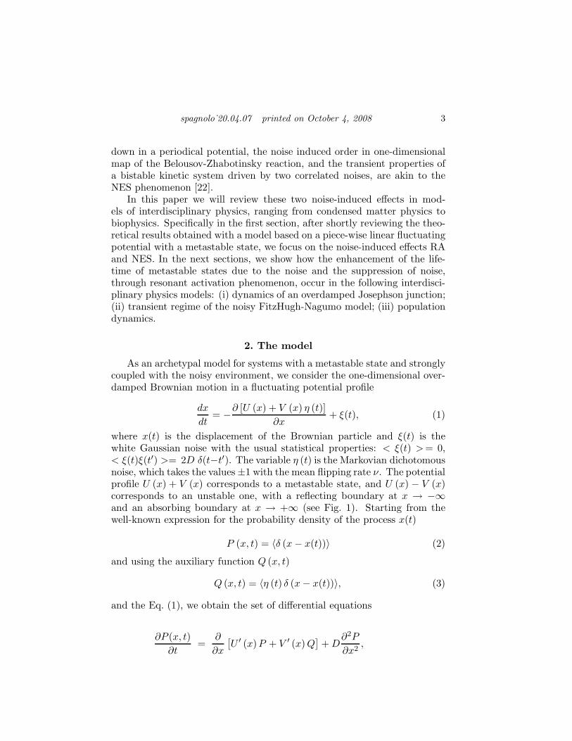
As an archetypal model for systems with a metastable state and stronglycoupled with the noisy environment, we consider the one-dimensional over-damped Brownian motion in a fluctuating potential profile

dx

dt= −∂ [U (x) + V (x) η (t)]

∂x+ ξ(t), (1)

where x(t) is the displacement of the Brownian particle and ξ(t) is thewhite Gaussian noise with the usual statistical properties: < ξ(t) > = 0,< ξ(t)ξ(t′) >= 2D δ(t−t′). The variable η (t) is the Markovian dichotomousnoise, which takes the values ±1 with the mean flipping rate ν. The potentialprofile U (x) + V (x) corresponds to a metastable state, and U (x) − V (x)corresponds to an unstable one, with a reflecting boundary at x → −∞and an absorbing boundary at x → +∞ (see Fig. 1). Starting from thewell-known expression for the probability density of the process x(t)

P (x, t) = 〈δ (x − x(t))〉 (2)

and using the auxiliary function Q (x, t)

Q (x, t) = 〈η (t) δ (x − x(t))〉, (3)

and the Eq. (1), we obtain the set of differential equations

∂P (x, t)

∂t=

∂

∂x

[

U ′ (x)P + V ′ (x) Q]

+ D∂2P

∂x2,


U(x)-V(x)

U(x)+V(x)

Fig. 1. Switching potential with metastable state.

∂Q(x, t)

∂t= −2νQ +

∂

∂x

[

U ′ (x)Q + V ′ (x) P]

+ D∂2Q

∂x2. (4)

The average lifetime of Brownian particles in the interval (L1, L2), with theinitial conditions P (x, 0) = δ (x − x0) and Q (x, 0) = ±δ (x − x0), is

τ (x0) =

∫ ∞

0dt

∫ L2

L1

P (x, t |x0, 0) dx =

∫ L2

L1

Y (x, x0, 0) dx , (5)

where Y (x, x0, s) is the Laplace transform of the conditional probabilitydensity P (x, t |x0, 0). After Laplace transforming Eqs. (4), with above-mentioned initial conditions and using the method proposed in Refs. [25,26, 30], we can express the lifetime τ(x0) as

τ (x0) =

∫ L2

L1

Z1 (x, x0) dx, (6)

where Z1(x, x0) is the linear coefficient of the expansion of the functionsY (x, x0, s) in a power series in s. By Laplace transforming the auxiliaryfunction Q(x, t) in R(x, x0, s), and expanding the function sR(x, x0, s) insimilar power series, we obtain the following closed set of integro-differentialequations for the functions Z1 (x, x0) and R1 (x, x0) [17]

DZ ′1 + U ′ (x)Z1 + V ′ (x)R1 = −θ (x − x0) ,

DR′1 + U ′R1 + V ′Z1 = 2ν

∫ x

−∞R1dy ∓ θ (x − x0) , (7)

where θ(x − x0) is the Heaviside step function, and R1 (x, x0) is the linearcoefficient of the expansion of the function sR(x, x0, s). We put equal tozero the probability flow at the reflecting boundary x = −∞. These general


equations (6) and (7) allow to calculate the average lifetime for potentialprofiles with metastable states. We may consider two mean lifetimes τ+ (x0)and τ− (x0), depending on the initial configuration of the randomly switch-ing potential profile: U (x) + V (x) or U (x) − V (x). The average lifetime(6) is equal to τ+ (x0), when we take the sign ”−” in the second equationof system (7), and vice versa for τ− (x0).

We consider now the following piece-wise linear potential profile

U(x) =

+∞, x < 00, 0 ≤ x ≤ Lk (L − x) , x > L

(8)

and V (x) = ax (x > 0, 0 < a < k). Here we consider the interval L1 =0, L2 = b, with b > L. After solving the differential equations (7) withthe potential profile (8), and by choosing the initial position of Brownianparticles at x = 0, we get the exact mean lifetime

τ− (xin = 0) =b

k+

νL2

Γ2+

a

2νΓ4f(D,Γ, ν), (9)

where Γ =√

a2 + 2νD. Here f(D,Γ, ν), which is also a function of thepotential parameters a, b, L, k, has a complicated expression in terms ofparameters D,Γ and ν [17]. It is worthwhile to note that Eq. (9) wasderived without any assumptions on the white noise intensity D and on themean rate of flippings ν of the potential.

To look for the NES effect, which is observable at very small noise in-tensity [3, 23], we derive the average life time in the limit D → 0

τ− (xin = 0) = τ0 +D

a2g(q, ω, s) + o (D) , (10)

where ω = νL/k, q = a/k and s = 2ω (b/L − 1) /(

1 − q2)

are dimensionlessparameters. Here

g(q, ω, s) =3q2 + 4q − 5

2(1 − q2)+ 2ω

3q2 + q − 3

q(1 − q2)− 2ω2

q2

+se−s q3(1 + q2)

(1 + q)(1 − q2)+

(

1 − e−s) q(1 − q2 − 2q3)

2(1 − q2)(11)

and

τ0 =2L

a+

νL2

a2+

b − L

k− q(1 − q)

2ν

(

1 − e−s) (12)


1.8

1.6

1.4

1.2

1-3 -2.5 -1.5-2 -1 -0.5 0

τ0

D

3

2

1

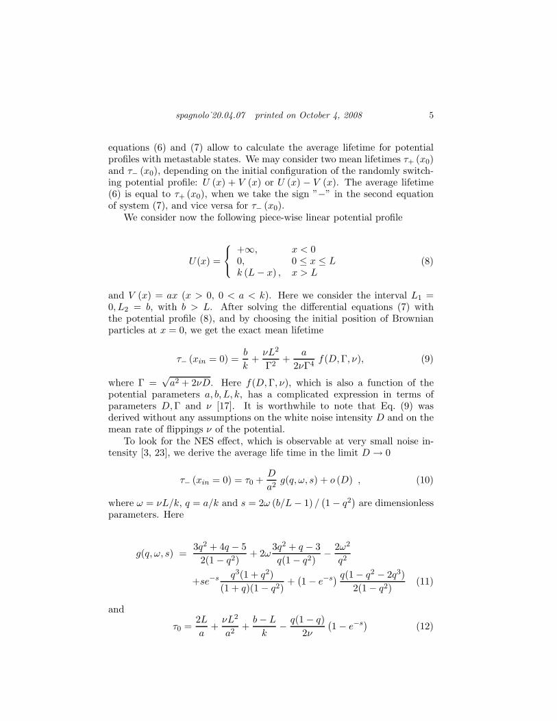
t_(xin=0)

Fig. 2. Semilogarithmic plot of the normalized mean lifetime τ− (xin = 0) /τ0 vs

the white noise intensity D for three values of the dimensionless mean flipping rate

ω = νL/k: 0.03 (curve 1), 0.01 (curve 2), 0.005 (curve 3). Parameters are L = 1,

k = 1, b = 2, and a = 0.995.

is the mean lifetime in the absence of white Gaussian noise (D = 0). Thecondition to observe the NES effect can be expressed by the inequality

g (q, ω, s) > 0. (13)

The main conclusions from the analysis of the inequality (13) are: (i) theNES effect occurs at q ≃ 1, i.e. at very small steepness k − a = k (1 − q)of the reverse potential barrier for the metastable state: for this potentialprofile, a small noise intensity can return particles into potential well, afterthey crossed the point L; (ii) for a fixed mean flipping rate, the NES effectincreases when q → 1, and (iii) for fixed parameter q the effect increaseswhen ω → 0, because Brownian particles have enough time to move backinto potential well.

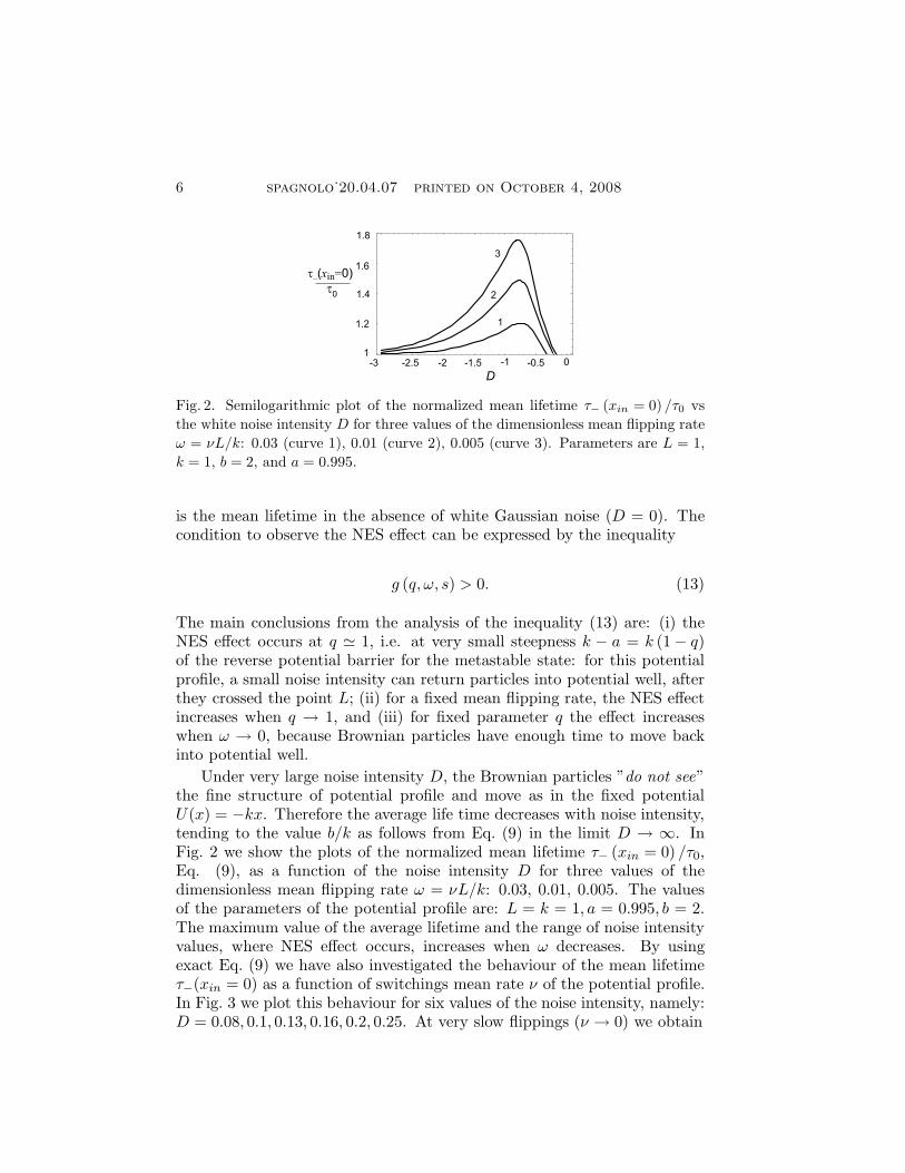
Under very large noise intensity D, the Brownian particles ”do not see”the fine structure of potential profile and move as in the fixed potentialU(x) = −kx. Therefore the average life time decreases with noise intensity,tending to the value b/k as follows from Eq. (9) in the limit D → ∞. InFig. 2 we show the plots of the normalized mean lifetime τ− (xin = 0) /τ0,Eq. (9), as a function of the noise intensity D for three values of thedimensionless mean flipping rate ω = νL/k: 0.03, 0.01, 0.005. The valuesof the parameters of the potential profile are: L = k = 1, a = 0.995, b = 2.The maximum value of the average lifetime and the range of noise intensityvalues, where NES effect occurs, increases when ω decreases. By usingexact Eq. (9) we have also investigated the behaviour of the mean lifetimeτ−(xin = 0) as a function of switchings mean rate ν of the potential profile.In Fig. 3 we plot this behaviour for six values of the noise intensity, namely:D = 0.08, 0.1, 0.13, 0.16, 0.2, 0.25. At very slow flippings (ν → 0) we obtain


t_(xin=0)

w-8 -6 -4 -2 0 2

10

8

6

4

2

0

Fig. 3. Semilogarithmic plot of the mean lifetime τ− (0) vs the dimensionless mean

flipping rate ω = νL/k for seven noise intensity values. Specifically from top to

bottom on the right side of the figure: D = 0.08, 0.1, 0.13, 0.16, 0.2, 0.25. The other

parameters are the same as in Fig. 2.

τ−(ν→0)(xin = 0) ≃ τd −D

(

1 − e−aL/D)

a2 (1 + q), (14)

i.e. the average lifetime of the fixed unstable potential U(x) − ax. Hereτd = L/a + (b − L)/(k + a) is the deterministic time at zero frequency(ν = 0). While for very fast switchings (ν → ∞) we obtain

τ−(ν→∞)(xin = 0) ≃ b

k+

L2

2D, (15)

i.e. the mean lifetime for average potential U (x). All limiting values ofτ−(xin = 0), expressed by Eqs. (14) and (15), are shown in Fig. 3. At in-termediate rates the average escape time from the metastable state exhibitsa minimum at ω = 0.1, which is the signature of the resonant activation(RA) phenomenon [11]-[15]. If the potential fluctuations are very slow, theaverage escape time is equal to the average of the crossing times over upperand lower configurations of the barrier, and the slowest process determinesthe value of the average escape time [11]. In the limit of very fast fluctu-ations, the Brownian particle ”sees” the average barrier and the averageescape time is equal to the crossing time over the average barrier. In theintermediate regime, the crossing is strongly correlated with the potentialfluctuations and the average escape time exhibits a minimum at a resonantfluctuation rate. Specifically, for D ≪ 1 and the parameter values of thepotential (a = 0.995, L = k = 1, b = 2), we obtain from Eqs. (14) and (15):τ−(ν→0)(xin = 0) ≃ 1.5 − D/2, and τ−(ν→∞)(xin = 0) ≃ 2 + 1/(2D), that is

τ−(ν→0)(xin = 0) ≪ τ−(ν→∞)(xin = 0) (16)


which is consistent with the physical picture for which we have at zerofrequency of switchings the unstable initial configuration of the potential(see Fig. 1), and at very fast switchings (ν → ∞) the average configurationof the potential, which in our case has not barrier. For D ≫ 1, because

limD→∞

D(

1 − e−aL/D)

= aL , (17)

we have τ−(ν→0)(xin = 0) = b/(k + a) ≃ 1, and τ−(ν→∞)(xin = 0) = 2. So,for the noise intensity values used in our calculations shown in Fig. 3, rangingfrom D = 0.08 to D = 0.25, the limiting values for the average lifetime are:τ−(ν→0)(xin = 0) ≃ (1.38÷1.46), and τ−(ν→∞)(xin = 0) ≃ (4÷8), which areconsistent with the limiting values shown in Fig. 3, and evaluated directlyfrom exact expression (9).

Moreover, in Fig. 3 a new resonance-like behaviour, is observed. Themean lifetime of the metastable state τ−(xin = 0) exhibits a maximum,between the slow limit of potential fluctuations (static limit) and the RAminimum, as a function of the mean fluctuation rate of the potential, . Thismaximum occurs for a value of the barrier fluctuation rate on the order ofthe inverse of the time τup(D) required to escape from the metastable fixedconfiguration

τup (D) =b − L

k − a− L

a+

D(

eaL/D − 1)

a2 (1 − q). (18)

Specifically we observe that this maximum increases with decreasing noiseintensity D and at the same time the position of the maximum is shiftedtowards lower values of the dimensionless mean flipping rate ω. In factfrom Eq. (18) we have that the average time required to escape from themetastable fixed configuration τup increases, consequently the correspondingrate of the barrier fluctuations ωmax ≃ 1/τup(D) decreases, as shown inFig. 3. We can also estimate the value of the maximum (τ−max(xin = 0))and its position (ωmax), by expanding Eqs. (10)-(12) in a power series upto the second order in ω. Using the same parameter values of the potential

we have: ω = ν, s = 2ω/(1 − q2), se−s ≈ s − s2, and 1 − e−s ≈ s − s2

2 . Weobtain finally:

τ− (xin = 0) ≈ 2.5 + (98.7)D + ω[51 + (347.4)D] − (2 × 106)ω2D . (19)

For D = 0.1 we have: τ−max ≈ 12.3 and ωmax ≈ 2 × 10−4, which are anestimate of the coordinates of the maximum of the corresponding curvein Fig. 3. From small noise intensity D → 0, from Eq. (19), we obtain:

τ−max ≈ 0.6×10−3

D + O(D). The maximum of the average lifetime τ−max,therefore, increases when the noise intensity decreases as shown in Fig. 3.


This suggests that, the enhancement of stability of metastable state isstrongly correlated with the potential fluctuations, when the Brownian par-ticle ”sees” the barrier of the metastable state [3, 17, 23]. When the averagetime to cross the barrier, that is the average lifetime of the metastable state,is approximately equal to the correlation time of the fluctuations of the po-tential barrier, a resonance-like phenomenon occurs. In other words, thisnew effect can be considered as a NES effect in the frequency domain. It isworthwhile to note that the new nonmonotonic behaviour shown in Fig. 3is in good agreement with experimental results observed in a periodicallydriven Josephson junction (JJ) [20]. In this very recent paper the authorsexperimentally observe the coexistence of RA and NES phenomena. Specif-ically they found (see Fig.3 of the paper [20]) that the maximum increaseswith decreasing bias current and at the same time the position of the max-imum is shifted towards lower values of ω. A decrease of the bias currentcauses (see next section on transient dynamics of a JJ) a decrease of theslope of the potential profile, which corresponds to a decreasing parame-ter k in our model (Eq. (8)). Therefore, the average lifetime maximumτ−max increases and as a consequence the time required to escape from themetastable fixed configuration τup(D) increases too. Consequently, the cor-responding rate of the barrier fluctuations ωmax ≃ 1/τup(D) decreases, asobserved experimentally. Of course a more detailed analysis of the JJ sys-tem as a function of the temperature, that is the noise intensity, should addmore interesting results.

Finally we note that in the frequency range ω ∈ (10−5 ÷ 10−3), for fixedvalues of the mean flipping rate, an overlap occurs in the curves for differentvalues of the noise intensity. A nonmonotonic behavior of τ−(xin = 0) asa function of the noise intensity is observed, as we expect in the transientdynamics of metastable states [3, 17, 23].

3. Transient dynamics in a Josephson junction

The investigation of thermal fluctuations and nonlinear properties ofJosephson junctions (JJs) is very important owing to their broad applica-tions in logic devices. Superconducting devices, in fact, are natural qubitcandidates for quantum computing because they exhibit robust, macro-scopic quantum behavior [31]. Recently, a lot of attention was devotedto Josephson logic devices with high damping because of their high-speedswitching [18, 32]. The rapid single flux quantum logic (RSFQ), for exam-ple, is a superconductive digital technique in which the data are representedby the presence or absence of a flux quantum Φ0 = h/2e, in a cell whichcomprises Josephson junctions. The short voltage pulse corresponds to asingle flux quantum moving across a Josephson junction, that is a 2π phase


flip. This short pulse is the unit of information. However the operatingtemperatures of the high-Tc superconductors lead to higher noise levelsby increasing the probability of thermally-induced switching errors. More-over during the propagation within the Josephson transmission line fluxonaccumulates a time jitter. These noise-induced errors are one of the mainconstraints to obtain higher clock frequencies in RSFQ microprocessors [32].

In this section, after a short introduction with the basic formulas ofthe Josephson devices, the model used to study the dynamics of a shortoverdapmed Josephsonn junction is described. The interplay of the noise-induced phenomena RA and NES on the temporal characteristics of theJosephson devices is discussed. The role played by these noise-induced ef-fects, in the accumulation of timing errors in RSFQ logic devices, is ana-lyzed.

The Josephson tunneling junction is made up of two superconductors,separated from each other by a thin layer of oxide. Starting from Schrodingerequation and the two-state approximation model [33], it is straightforwardto obtain the Josephson equation

dϕ(t)

dt=

2eV (t)

h, (20)

where ϕ is the phase difference between the wave function for the left andright superconductors, V (t) is the potential difference across the junction,e is the electron charge, and h = h/2π is the Planck’s constant. A smalljunction can be modelled by a resistance R in parallel with a capacitanceC, across which is connected a bias generator and a phase-dependent cur-rent generator, Isinϕ, representing the Josephson supercurrent due to theCooper pairs tunnelling through the junction. Since the junction oper-ates at a temperature above absolute zero, there will be a white Gaussiannoise current superimposed on the bias current. Therefore the dynamicsof a short overdamped JJ, widely used in logic elements with high-speedswitching and corresponding to a negligible capacitance C, is obtained fromEq. (20) and from the current continuity equation of the equivalent circuitof the Josephson junction. The resulting equation is the following Langevinequation

ω−1c

dϕ(t)

dt= −du(ϕ)

dϕ− iF (t), (21)

valid for β ≪ 1, with β = 2eIcR2C/h the McCamber–Stewart parameter,

Ic the critical current, and iF (t) =IF

Ic, with IF the random component of

the current. Here

https://www.researchgate.net/publication/247181180_Physics_and_Application_of_the_Josephson_Effect?el=1_x_8&enrichId=rgreq-9bfb3974c0f18852dd64e9d8b0fd8bd4-XXX&enrichSource=Y292ZXJQYWdlOzIyMDkwNjc7QVM6MTA0MTM1NzMwOTI1NTc3QDE0MDE4MzkzMDIwMTM=


u(ϕ, t) = 1 − cosϕ − i(t)ϕ, with i(t) = i0 + f(t), (22)

is the dimensionless potential profile (see Fig. 4), ϕ is the difference in thephases of the order parameter on opposite sides of the junction, f(t) =

A sin(ωt) is the driving signal, i =I

Ic, ωc =

2eRN Ic

his the characteristic

frequency of the JJ, and RN is the normal state resistance (see Ref. [33]).When only thermal fluctuations are taken into account [33], the randomcurrent may be represented by the white Gaussian noise: 〈iF (t)〉 = 0,

〈iF (t)iF (t + τ)〉= 2D

ωcδ(τ), where D =

2ekT

hIc=

IT

Icis the dimensionless

intensity of fluctuations, T is the temperature and k is the Boltzmann con-stant. The equation of motion Eq. (21) describes the overdamped motion

-10 -6 -2 2 6 10j

-10

-5

0

5

10

u(j)

Fig. 4. The potential profile u(ϕ) = 1−cosϕ− iϕ, for values of the current, namely

i = 0.5 (solid line) and i = 1.2 (dashed line).

of a Brownian particle moving in a washboard potential (see Fig. 4). Ajunction initially trapped in a zero-voltage state, with the particle localizedin one of the potential wells, can escape out of the potential well by ther-mal fluctuations. The phase difference ϕ fluctuates around the equilibriumpositions, minima of the potential u(ϕ), and randomly performs jumps of2π across the potential barrier towards a neighbor potential minimum. Theresulting time phase variation produces a nonzero voltage across the junc-tion with marked spikes. For a bias current less than the critical currentIc, these metastable states correspond to ”superconductive” states of theJJ. The mean time between two sequential jumps is the life time of thesuperconductive metastable state [25]. For an external current greater thanIc, the JJ junction switches from the superconductive state to the resistiveone and the phase difference slides down in the potential profile, which now




has not equilibrium steady states. A Josephson voltage output will be gen-erated in a later time. Such a time is the switching time, which is a randomquantity. In the presence of thermal noise a Josephson voltage appears evenif the current is less than the critical one (i < 1), therefore we can identifythe lifetime of the metastable states with the mean switching time [18, 25].For the description of our system, i. e. a single overdamped JJ with noise,we will use the Fokker-Planck equation for the probability density W (ϕ, t),which corresponds to the Langevin equation (21)

∂W (ϕ, t)

∂t= −∂G(ϕ, t)

∂ϕ= ωc

∂

∂ϕ

du(ϕ)

dϕW (ϕ, t) + D

∂W (ϕ, t)

∂ϕ

. (23)

The initial and boundary conditions of the probability density and of theprobability current for the potential profile (22) are as follows: W (ϕ, 0) =δ(ϕ − ϕ0), W (+∞, t) = 0, G(−∞, t) = 0. Let, initially, the JJ is biasedby the current smaller than the critical one, that is i0 < 1, and the junc-tion is in the superconductive state. The current pulse f(t), such thati(t) = i0 + f(t) > 1, switches the junction into the resistive state. Anoutput voltage pulse will appear after a random switching time. We willcalculate the mean value and the standard deviation of this quantity fortwo different periodic driving signals: (i) a dichotomous signal, and (ii) asinusoidal one. We will consider different values of the bias current io andof signal amplitude A. Depending on the values of io and A, as well asvalues of signal frequency and noise intensity, two noise-induced effects maybe observed, namely the resonant activation (RA) and the noise enhancedstability (NES). Specifically the RA effect was theoretically predicted inRef. [11] and experimentally observed in a tunnel diode [13] and in un-derdamped Josephson tunnel junctions [16, 20], and the NES effect wastheoretically predicted in [22, 23, 25] and experimentally observed in a tun-nel diode [3] and in an underdamped Josephson junction [20]. The RA andNES effects, however, have different role on the behavior of the temporalcharacteristics of the Josephson junction. They occur because of the pres-ence of metastable states, in the periodic potential profile of the Josephsontunnel junction, and the thermal noise. Specifically, the RA phenomenonminimizes the switching time and therefore also the timing errors in RSFQlogic devices, while the NES phenomenon increases the mean switching timeproducing a negative effect [18].

3.1. Temporal characteristics

Now we investigate the following temporal characteristics: the meanswitching time (MST) and its standard deviation (SD) of the Josephson


junction described by Eq. (21). These quantities may be introduced as char-

acteristic scales of the evolution of the probability P (t) =ϕ2∫

ϕ1

W (ϕ, t)dϕ, to

find the phase within one period of the potential profile of Eq. (22). Wechoose therefore ϕ2 = π, ϕ1 = −π and we put the initial distribution on thebottom of a potential well: ϕ0 = arcsin(i0). A widely used definition of suchcharacteristic time scales is the integral relaxation time (see the paper byMalakhov and Pankratov in Ref [12]). Let us summarize shortly the resultsobtained in the case of dichotomous driving, f(t) = Asign(sin(ωt)). BothMST and its SD do not depend on the driving frequency below a certaincut-off frequency (approximately 0.2ωc), above which the characteristics de-grade. In the frequency range from 0 to 0.2ωc, therefore, we can describe theeffect of dichotomous driving by time characteristics in a constant potential.The exact analytical expression of the first two moments of the switchingtime are [18]

τc(ϕ0) =1

Dωc

ϕ2∫

ϕ0

eu(x)

D

x∫

ϕ1

e−u(ϕ)

D dϕdx +

ϕ2∫

ϕ1

e−u(ϕ)

D dϕ

∞∫

ϕ2

eu(ϕ)

D dϕ

, (24)

and

τ2c(ϕ0) = τ2c (ϕ0) −

∫ ϕ2

ϕ0

e−u(x)

D H(x)dx − H(ϕ0)

∫ ϕ0

ϕ1

e−u(x)

D dx, (25)

where H(x) = 2(Dωc)2

∞∫

xeu(v)/D

ϕ2∫

ve−u(y)/D

∞∫

yeu(z)/Ddzdydv. The asymptotic

expressions of the MST and its standard deviation (SD), obtained in thesmall noise limit (D ≪ 1), agree very well with computer simulations up toD = 0.05 [18]. Therefore, not only low temperature devices (D ≤ 0.001),but also high temperature devices may be described by these expressions. Ifthe noise intensity is rather large, the phenomenon of NES may be observedin our system: the MST increases with the noise intensity. Here we notethat it is very important to consider this effect in the design of large arraysof RSFQ elements, operating at high frequencies. To neglect this noise-induced effect in such nonlinear devices it may lead to malfunctions due tothe accumulation of errors.

Now let us consider the case of sinusoidal driving. The correspondingtime characteristics may be derived using the modified adiabatic approxi-mation [14, 18]

P (ϕ0, t) = exp

−∫ t

0

1

τc(ϕ0, t′)dt′

, (26)


with τc(ϕ0, t′) given by Eq. (24), after inserting in this equation the time

dependent potential profile u(ϕ, t) of Eq. (22). Using the relation τ =∫ +∞0 P (ϕ0, t)dt we calculate the MST. We focus now on the current value

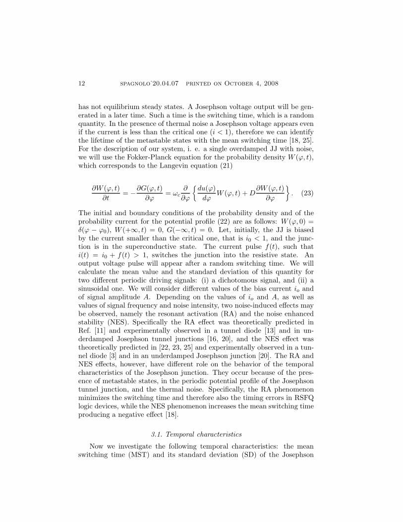
i = 1.5, because i = 1.2 is too small for high frequency applications. InFig. 5 the MST and its SD as a function of the driving frequency, for threevalues of the noise intensity (D = 0.02, 0.05, 0.5), for a bias current i0 = 0.5,and A = 1 are shown. We note that, because ϕ0 = arcsin(i0) depends oni0, the switching time is larger for smaller i0. However, great bias currentvalues i0, in the absence of driving, give rise to the reduction of the mean lifetime of superconductive state, i.e. to increasing storage errors (Eq. (24)).Therefore, there must be an optimal value of bias current i0, giving min-imal switching time and acceptably small storage errors. We observe thephenomenon of resonant activation: MST has a minimum as a function ofdriving frequency.

0.1 1w

1

10

t(w),s(w)

D=0.02

D=0.05

D=0.5

s

t

Fig. 5. The MST and its SD vs frequency for f(t) = A sin(ωt) (computer simula-

tions) for three values of the noise intensity. Namely: Long-dashed line - D = 0.02,

short-dashed line - D = 0.05, solid line - D = 0.5. The value of the bias current is

i0 = 0.5, and the total current is i = 1.5.

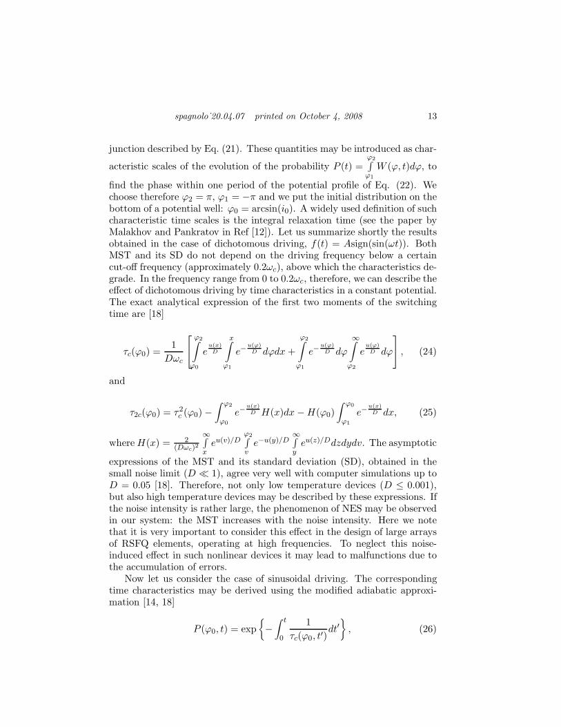
The approximation (26) works rather well below 0.1 ωc, that is enoughfor practical applications (see the inset of Fig. 3 in ref. [18]). It is interestingto see that near the minimum the MST has a very weak dependence onthe noise intensity (as it is clearly shown in the τ behavior of Fig. 5 forthree values of the noise intensity), i. e. in this signal frequency rangethe noise is effectively suppressed. This noise suppression is due to theresonant activation phenomenon: a minimum appears in the MST and SD,when the escape process is strongly correlated with the potential profileoscillations. A noise suppression effect, but due to the noise, is reportedin Ref. [34]. We observe also the NES phenomenon. There is a frequencyrange in Fig. 5, around (0.2 ÷ 0.48)ωc for i0 = 0.5, where the switching


0.01 0.1 1 10

D

0

10

20

t(D)

0.01 0.1 1 10

D

0

5

10

s(D)

w=0.1

w=0.3

w=0.4

Fig. 6. The MST vs noise intensity for f(t) = A sin(ωt) and for three values of

the driving frequency. Namely: ω = 0.1 (long-dashed line), ω = 0.3 (short-dashed

line), ω = 0.4 (solid line). Inset: The standard deviation (SD) vs noise intensity

for the same values of driving frequency ω.

time increases with the noise intensity. To see in more detail this effect wereport in Fig. 6 the MST τ(D) and its SD σ(D) vs the noise intensity D, forthree fixed values of the driving frequency, namely: ω = 0.1, 0.3, 0.4. Bothquantities have nonmonotonic behaviour and the great values of σ(D) nearthe maximum of τ(D) confirm that the only information on the MST is notsufficient to fully unravel the statistical properties of the NES effect [24]. Adetailed analysis of the PDF of the lifetime during the transient dynamics isrequired. This is subject of a forthcoming paper. Simulations for differentbias current values [18] show that the NES effect increases for smaller i0because the potential barrier disappears for a short time interval withinthe driving period T = 2π/ω and the potential is more flat [3]. The noise,therefore, has more chances to prevent the phase to move down and theswitching process is delayed. This effect may be avoided, if the operatingfrequency does not exceed 0.2 ωc. Besides the SD and MST (see Fig. 5)have their minima in a short range of values of ω [18]. Close location ofminima of MST and its SD means that optimization of RSFQ circuit forfast operation will simultaneously lead to minimization of timing errors inthe circuit.

4. Dynamics of a FHN stochastic model

4.1. Suppression of noise and noise-enhanced stability effect

Case I. Let us fix the value of the noise intensity and analyze The analy-sis of the stochastic properties of neural systems is of particular importancesince it plays an important role in signal transmission [19], [35]-[41]. Bio-


logically realistic models of the nerve cells, such as widely-known Hodgkin-Huxley (HH) system [35], are so complex that they provide little intuitive in-sight into the neuron dynamics that they simulate. The FitzHugh-Nagumo(FHN) model, however, which is one of the simplified modifications of HH,is more preferable for investigation [41]. Nevertheless many effects observedin neural cells are qualitatively contained in FHN model. Because of thisthe FHN model has got wide dissemination in the last few years. Therehas been a lot of papers where the influence of noise on the encoding sen-sitivity of a neuron in the framework of FHN model has been analyzed. Abroad spectrum of noise-induced dynamical effects, which produce orderedperiodicity in the output of the FHN system, has been discovered. Amongthese effects we cite the coherence resonance [36] and the stochastic reso-nance (SR) [37]. All these investigations deal with neuron dynamics withsubthreshold signals, and with an enhancement of a weak signal through thenoise. The presence of noise in the case of a strong periodic forcing, however,has a detrimental effect on the encoding process [38]-[40]. For suprathresh-old signals the noise always lowers the information transmission, and theSR effects disappear [38, 39]. However, as it was shown in recent papersof Stocks [40], this is only true for a single element threshold system. Inneuronal arrays the noise can significantly enhance the information trans-mission when the signal is predominantly suprathreshold. It is the effect ofsuprathreshold stochastic resonance.

Here we analyze the effect of noise in a single neuron subjected to astrong periodic forcing. We investigate therefore, the influence of noise onthe appearance time of a first spike, or the mean response time, in theoutput of FHN model with periodical driving in suprathreshold regime. Asit was mentioned before, the role of noise for a strong driving is negative.In this case noise suppresses the response of a neuron, that leads to delayof transmission of an external information. But we show that, this negativeinfluence of noise on the spike generation can be significantly minimized.

We analyze the dependencies of the mean response time (MRT) on bothdriving frequency and noise intensity. We find that, MRT plotted as a func-tion of the driving frequency shows a resonant activation-like phenomenon.The noise enhanced stability (NES) effect is also observed here. It is shownthat MRT can be increased due to the effect of fluctuations. We note thatNES has nothing to do with the typical SR, where the maximum of signalto noise ratio as a function of noise intensity is observed. There are manydifferences between these effects concerning the neuron dynamics. First ofall the SR is related to the output of the neuron in stationary dynamicalregime and concerns the signal-to-noise ratio, while the NES describes thetransient dynamical regime of a neuron and concerns the mean responsetime. In addition there is difference in the nature of the response: We


investigate the case of a strong driving, where the SR effects disappear.

4.2. Deterministic dynamical regime

The dynamic equations of the FitzHugh-Nagumo model with additiveperiodic forcing are

x = x − x3/3 − y + A sin(ωt)y = ǫ(x + I),

(27)

where x is the voltage, y is the recovery variable, and ǫ is a fixed smallparameter (ǫ = 0.05). In the absence of both external driving and noise,there is only one steady state of the system (27), that is x0 = −I; y0 =−I+I3/3. The choice of the constant I, therefore, fully specifies the locationof equilibrium state in the phase space (x, y). Here we consider I = 1.1.

In our simulations we assume that the initial conditions for each real-ization are the same, that is the system is in its stable equilibrium point(the rest state) (x0, y0) at the initial time t0. We would like to note, here,that even if we consider sinusoidal driving, we investigate the time of ap-pearance of the first spike only. We are interested in the capability of oursystem to detect an external input. This means to minimize the detectiontime and to get a neuron response that would be more robust to the noiseaction. After generation of the first spike, that is after approaching of theboundary x = 0, we break the realization off, and start a new one with thesame initial conditions (x0, y0).

For our system the threshold value of the driving amplitude required forspike generation is Ath ∼ 0.05. In our simulations we choose A = 0.5. Thus,the frequency range where the signal of such amplitude is suprathresholdis: Ω : ω ∈ (0.013 ÷ 1.9) [19]. Inside this region Ω the response time of aneuron has a minimum as a function of the driving frequency. System doesnot respond outside the range Ω. Here, a subthreshold oscillation occurs(see Fig. 7(b)). In Fig. 7(c) the time series of the output voltage x for asuprathreshold signal is shown.

4.3. Suprathreshold stochastic regime

Actually, there are many factors that make the environment noisy inthe neuron dynamics. Among them we cite the fluctuating opening andclosure of the ion channels within the cell membrane, the noisy presynapticcurrents, and others (see, for example, Ref. [36]). We consider two differentcases in which the noise is added to the first or the second equation of thesystem (27):


1E-3 0.01 0.1 1 100

5

10

15

20

-1.5

-1.0

-0.5

0 200 400 600 800 1000

-2-1012

(a)

(b)

x

(c)

x

t

Fig. 7. (a) The response time dependence versus the frequency of periodic driving

for the deterministic case, A = 0.5. Examples of output trajectory for two values

of driving frequency invoking two different kinds of oscillations: (b) subthreshold

for ω = 0.01, and (c) suprathreshold for ω = 0.02.

Case I The variable that corresponds to the membrane potential is sub-jected to fluctuations [37, 40]. In this case, the first equation of the sys-tem (27) becomes the following stochastic differential equation

x = x − x3/3 + A sin(ωt) − y + ξ(t); (28)

Case II The recovery variable associated with the refractory propertiesof a neuron is noisy [36]. Here, the second equation of the system (27)becomes

y = ǫ(x + I) + ξ(t), (29)

In Eqs. (28) and (29), ξ(t) is a Gaussian white noise with zero mean andcorrelation function 〈ξ(t)ξ(t + τ)〉 = Dδ(τ). For numerical simulations weuse the modified midpoint method and the noise generator routine reportedin Ref [42].

The mean response time (MRT) of our neuronal system is obtained asthe mean first passage time at the boundary x = 0: τ =< T >= 1

N

∑Ni=1 Ti,

where Ti is the response time for i-th realization. To obtain smooth averagefor all the noise values investigated, we need different number of realizationsN in above considered cases. Namely, N = 5000 in case I, and N = 15000in case II, specifically when the noise intensities are comparable with thevalue of the parameter ǫ = 0.05. It is worth noting here that parameter Ti

characterizes the delay of the systems’ response, and has a non-zero valueeven in the deterministic case, because of the non-instantaneous neuronal


response. In our investigation we consider a strong driving, so the noiseincreases the time of appearance of the first spike and leads to an additionaldelay of the signal detection.

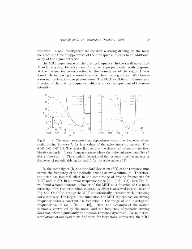
the MRT dependence on the driving frequency. In the small noise limitD → 0, a typical behavior (see Fig. 8) with perpendicular walls disposedat the frequencies corresponding to the boundaries of the region Ω wasfound. By increasing the noise intensity, these walls go down. We observea resonant activation-like phenomenon: The MRT exhibits a minimum as afunction of the driving frequency, which is almost independent of the noiseintensity.

0.0001 0.001 0.01 0.1 1 10

w

0

3

6

9

12

s

D=0.005

D=0.03

D=0.07

D=0.5

(b)

0.0001 0.001 0.01 0.1 1 10

w

0

5

10

15

20

25

t

D=0.005

D=0.03

D=0.07

D=0.5

0.5 1.0 1.5

2

3

4

(a)

Fig. 8. (a) The mean response time dependence versus the frequency of pe-

riodic driving for case I, for four values of the noise intensity, namely: D =

0.005, 0.03, 0.07, 0.5. The right solid lines give the theoretical values of τ for fixed

bistable potential. Inset: frequency range where the noise enhanced stability ef-

fect is observed. (b) The standard deviation of the response time dependence vs

frequency of periodic driving for case I, for the same values of D.

In the same figure (b) the standard deviation (SD) of the response timeversus the frequency of the periodic driving shows a minimum. Therefore,the noise has minimal effect in the same range of driving frequencies forMRT and its SD. In a narrow frequency range (ω ∈ (0.6÷1.3)) (see Fig. 8),we found a nonmonotonic behavior of the MRT as a function of the noiseintensity. Here the noise enhanced stability effect is observed (see the inset ofFig. 8a). Out of this range the MRT monotonically decreases with increasingnoise intensity. For larger noise intensities the MRT dependence on drivingfrequency takes a constant-like behavior in the range of the investigatedfrequency values (ω ∈ [10−4 ÷ 10]). Here, the dynamics of the systemis mainly controlled by the noise, and the frequency of periodic drivingdoes not affect significantly the neuron response dynamics. By numericalsimulations of our system we find that, for large noise intensities, the MRT


coincides with that calculated by standard technique for a Brownian particlemoving in a bistable fixed potential [44]

τ = 2/D

∫ 0

x0

eϕ(x)/D∫ x

∞e−ϕ(y)/Ddydx. (30)

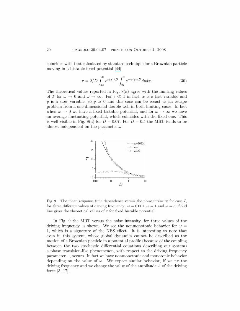
The theoretical values reported in Fig. 8(a) agree with the limiting valuesof T for ω → 0 and ω → ∞. For ǫ ≪ 1 in fact, x is a fast variable andy is a slow variable, so y ≃ 0 and this case can be recast as an escapeproblem from a one-dimensional double well in both limiting cases. In factwhen ω → 0 we have a fixed bistable potential, and for ω → ∞ we havean average fluctuating potential, which coincides with the fixed one. Thisis well visible in Fig. 8(a) for D = 0.07. For D = 0.5 the MRT tends to bealmost independent on the parameter ω.

0.01 0.1 1 10

0

5

10

15

20

w=0.001w=1w=5

t

D

Fig. 9. The mean response time dependence versus the noise intensity for case I,

for three different values of driving frequency: ω = 0.001, ω = 1 and ω = 5. Solid

line gives the theoretical values of τ for fixed bistable potential.

In Fig. 9 the MRT versus the noise intensity, for three values of thedriving frequency, is shown. We see the nonmonotonic behavior for ω =1, which is a signature of the NES effect. It is interesting to note thateven in this system, whose global dynamics cannot be described as themotion of a Brownian particle in a potential profile (because of the couplingbetween the two stochastic differential equations describing our system)a phase transition-like phenomenon, with respect to the driving frequencyparameter ω, occurs. In fact we have nonmonotonic and monotonic behaviordepending on the value of ω. We expect similar behavior, if we fix thedriving frequency and we change the value of the amplitude A of the drivingforce [3, 17].

https://www.researchgate.net/publication/224043701_Handbook_of_Stochastic_Methods?el=1_x_8&enrichId=rgreq-9bfb3974c0f18852dd64e9d8b0fd8bd4-XXX&enrichSource=Y292ZXJQYWdlOzIyMDkwNjc7QVM6MTA0MTM1NzMwOTI1NTc3QDE0MDE4MzkzMDIwMTM=


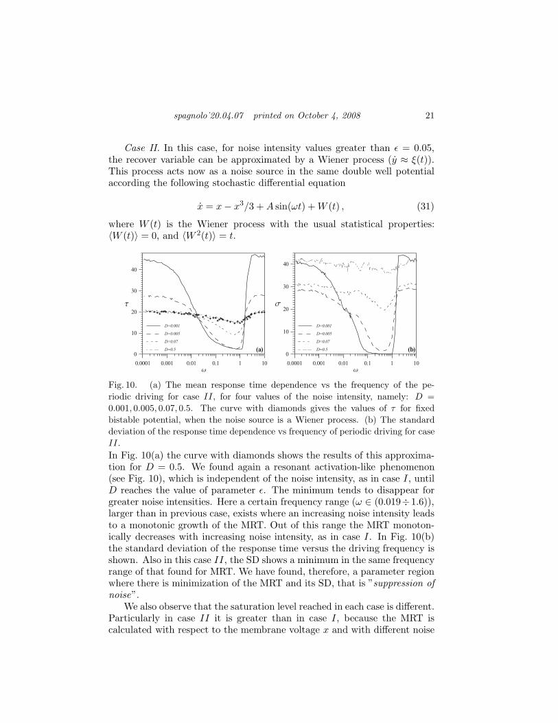
Case II. In this case, for noise intensity values greater than ǫ = 0.05,the recover variable can be approximated by a Wiener process (y ≈ ξ(t)).This process acts now as a noise source in the same double well potentialaccording the following stochastic differential equation

x = x − x3/3 + A sin(ωt) + W (t) , (31)

where W (t) is the Wiener process with the usual statistical properties:〈W (t)〉 = 0, and 〈W 2(t)〉 = t.

0.0001 0.001 0.01 0.1 1 10

w

0

10

20

30

40

s

D=0.001

D=0.005

D=0.07

D=0.5 (b)

0.0001 0.001 0.01 0.1 1 10

w

0

10

20

30

40

t

D=0.001

D=0.005

D=0.07

D=0.5 (a)

Fig. 10. (a) The mean response time dependence vs the frequency of the pe-

riodic driving for case II, for four values of the noise intensity, namely: D =

0.001, 0.005, 0.07, 0.5. The curve with diamonds gives the values of τ for fixed

bistable potential, when the noise source is a Wiener process. (b) The standard

deviation of the response time dependence vs frequency of periodic driving for case

II.

In Fig. 10(a) the curve with diamonds shows the results of this approxima-tion for D = 0.5. We found again a resonant activation-like phenomenon(see Fig. 10), which is independent of the noise intensity, as in case I, untilD reaches the value of parameter ǫ. The minimum tends to disappear forgreater noise intensities. Here a certain frequency range (ω ∈ (0.019÷1.6)),larger than in previous case, exists where an increasing noise intensity leadsto a monotonic growth of the MRT. Out of this range the MRT monoton-ically decreases with increasing noise intensity, as in case I. In Fig. 10(b)the standard deviation of the response time versus the driving frequency isshown. Also in this case II, the SD shows a minimum in the same frequencyrange of that found for MRT. We have found, therefore, a parameter regionwhere there is minimization of the MRT and its SD, that is ”suppression ofnoise”.

We also observe that the saturation level reached in each case is different.Particularly in case II it is greater than in case I, because the MRT iscalculated with respect to the membrane voltage x and with different noise


sources. Therefore, in phase space the variable x reaches, in case I, in aminor average time the boundary x = 0, according to Eq. (28). While incase II the variation of x depends on the dynamics of the y coordinate andtakes much more time to reach the same boundary.

5. A stochastic model for cancer growth dynamics

In this last section we shortly summarize some of the main results ob-tained with a stochastic model for cancer growth dynamics (see Ref. [21] formore details). Most of tumoral cells bear antigens which are recognized asstrange by the immune system. A response against these antigens may bemediated either by immune cells such as T-lymphocytes or other cells likemacrophages. The process of damage to tumor proceeds via infiltration ofthe latter by the specialized cells, which subsequently develop a cytotoxicactivity against the cancer cell-population. The series of cytotoxic reactionsbetween the cytotoxic cells and the tumor tissue have been documented tobe well approximated by a saturating, enzymatic-like process whose timeevolution equations are similar to the standard Michaelis-Menten kinet-ics [45, 46]. The T-helper lymphocytes and macrophages, can secrete cy-tokines in response to stimuli. The functions that cytokines induce can both”turn on” and ”turn off ” particular immune responses [47, 48]. This ”on-off ” modulating regulatory role of the cytokines is here modelled through adichotomous random variation of the parameter β, which is responsibile forregulatory inhibition of the population growth, by taking into account thenatural random fluctuations always present in biological complex systems.

The dynamical equation of this biological system is

x = −dU±(x)

dx+ ξ(t), (32)

where ξ(t) is a Gaussian process with 〈ξ(t)〉 = 0, 〈ξ(t)ξ(t′)〉 = Dδ(t − t′),and

U±(x) = −x2

2+

θx3

3+ (βo ± ∆)(x − ln(x + 1)), (33)

is the stochastic double well Michaelis-Menten potential with one the min-ima at x = 0. Here x(t) is the concentration of the cancer cells. The processβ = (βo ±∆) can change the relative stability of the metastable state of thepotential profile [46]. We note that the RA and NES phenomena act counterto each other in the cancer growth dynamics: the NES effect increases in anunavoidable way the average lifetime of the metastable state (associated toa fixed-size tumor state), while the RA phenomenon minimizes this lifetime.Therefore it is crucial to find the optimal range of parameters in which the


positive role of resonant activation phenomenon, with respect to the can-cer extinction, prevails over the negative role of NES, which enhances thestability of the tumoral state. These are just the main results of the pa-per [21], that is both NES and RA phenomena are revealed in a biologicalsystem with a metastable state, with a co-occurrence region of these effects.In this coexistence region the NES effect, which enhances the stability ofthe tumoral state, becomes strongly reduced by the RA mechanism, whichenhances the cancer extinction. In other words, an asymptotic regression tothe zero tumor size may be induced by controlling the modulating stochasticactivity of the cytokines on the immune system.

6. Conclusions

Natural systems are open to the environment. Consequently, in general,stationary states are not equilibrium states, but are strongly influenced bydynamics, which adds further challenge to the microscopic understandingof metastability. The investigation of two noise-induced effects in far fromequilibrium systems, namely the RA and NES phenomena, has revealedinteresting peculiarities of the dynamics of these systems. Specifically theknowledge of the parameter regions where the RA and NES can be revealedallows:

• to optimize and to suppress timing errors in practical RSFQ devices,and therefore to significantly increase working frequencies of RSFQcircuits;

• to optimize the operating range of a neuron, and therefore to realizehigh rate signal transmission with the suppression of noise;

• to maximize or minimize the extinction time in cancer growth popu-lation dynamics.

7. Acknowledgments

This work was supported by MIUR, INFM-CNR and CNISM, RussianFoundation for Basic Research (Projects No. 05-01-00509 and No. 05-02-19815), and ESF(European Science Foundation) STOCHDYN network.E.V.P. also acknowledges the support of the Dynasty Foundation.

REFERENCES

[1] J.D. Gunton, M. Droz, Introduction to the Theory of Metastable and UnstableStates, Springer, Berlin, 1983.


[2] A. J. Leggett, Phys. Rev. Lett. 53, 1096 (1984); M. Muthukumar, ibid. 86,3188 (2001).

[3] R. N. Mantegna and B. Spagnolo, Phys. Rev. Lett. 76, 563 (1996); Int. J.Bifurcation and Chaos 4, 783 (1998).

[4] A. Strumia, N. Tetradis, JHEP 11, 023 (1999).

[5] P.G. Debenedetti, F.H. Stillinger, Nature 410, 267 (2001).

[6] R. H. Victora, Phys. Rev. Lett. 63, 457 (1989).

[7] Y.W. Bai et al, Science 269, 192 (1995).

[8] O. A. Tretiakov, T. Gramespacher, and K. A. Matveev, Phys. Rev. B 67,073303 (2003).

[9] M. Gleiser, R.C. Howell, Phys. Rev. Lett. 94, 151601 (2005).

[10] G. Parisi, Nature 433, 221 (2005); S. Kraut and C. Grebogi, Phys. Rev. Lett.93, 250603 (2004); H. Larralde and F. Leyvraz, ibid. 94, 160201 (2005); G.Baez et al., ibid. 90, 135701 (2003).

[11] C. R. Doering and J. C. Gadoua, Phys. Rev. Lett. 69, 2318 (1992).

[12] M. Bier and R. D. Astumian, Phys. Rev. Lett. 71, 1649 (1993); P. Pechukasand P. Hanggi, ibidem 73, 2772 (1994); J. Iwaniszewski, Phys. Rev. E 54,3173 (1996); M. Boguna, J. M. Porra, J. Masoliver, and K. Lindenberg, ibidem57, 3990 (1998); M. Bier, I. Derenyi, M. Kostur, D. Astumian, ibidem 59,6422 (1999); A. L. Pankratov and M. Salerno, Phys. Lett. A 273, 162 (2000);A. N. Malakhov and A. L. Pankratov, Adv. Chem. Phys. 121, 357 (2002).

[13] R. N. Mantegna and B. Spagnolo, Phys. Rev. Lett. 84, 3025 (2000); J. Phys.IV (France) 8, 247 (1998).

[14] A. L. Pankratov and M. Salerno, Phys. Lett. A 273, 162 (2000).

[15] B. Dybiec, E. Gudowska–Nowak, Phys. Rev. E 66, 026123 (2002).

[16] Y. Yu and S. Han, Phys. Rev. Lett. 91, 127003 (2003).

[17] A. A. Dubkov, N. V. Agudov and B. Spagnolo, Phys. Rev. E 69, 061103(2004).

[18] A. L. Pankratov and B. Spagnolo, Phys. Rev. Lett. 93, 177001 (2004).

[19] E. V. Pankratova, A. V. Polovinkin, and B. Spagnolo, Physics Letters A 344,43-50 (2005).

[20] G. Sun et al., Phys. Rev. E 75, 021107(4) (2007).

[21] A. Fiasconaro and B. Spagnolo, A. Ochab-Marcinek and E. Gudowska-Nowak,Phys. Rev. E 74, 041904(10) (2006); A. Ochab-Marcinek, E. Gudowska-Nowak, A. Fiasconaro and B. Spagnolo, Acta Physica Polonica B 37 (5),1651 (2006).

[22] J. E. Hirsch, B. A. Huberman, and D. J. Scalapino, Phys. Rev. A 25, 519(1982); I. Dayan, M. Gitterman, and G. H. Weiss, ibidem 46, 757 (1992); R.Wackerbauer, Phys. Rev. E 59, 2872 (1999); D. Dan, M. C. Mahato, and A.M. Jayannavar, ibidem 60, 6421 (1999); A. Mielke, Phys. Rev. Lett. 84, 818(2000); C. Xie and D. Mei, Chin. Phys. Lett. 20, 813 (2003).

[23] N. V. Agudov and B. Spagnolo, Phys. Rev. E 64, 035102(R) (2001).


[24] A. Fiasconaro, B. Spagnolo and S. Boccaletti, Phys. Rev. E 72, 061110(5)(2005); A. Fiasconaro, D. Valenti, B. Spagnolo, Physica A 325, 136-143 (2003).

[25] A. N. Malakhov and A.L. Pankratov, Physica C 269, 46 (1996).

[26] N. V. Agudov and A. N. Malakhov, Phys. Rev. E 60, 6333 (1999).

[27] B. Spagnolo, A. A. Dubkov, and N. V. Agudov, Eur. Phys. J. B 40, 273-281(2004); B. Spagnolo, A. A. Dubkov, N. V. Agudov, Acta Physica Polonica B35, 1419 (2004).

[28] H. A. Kramers, Physica 7, 284 (1940).

[29] P. Hanggi, P. Talkner, and M. Borkovec, Rev. Mod. Phys. 62, 251 (1990).

[30] A. N. Malakhov, Chaos 7, 488 (1997).

[31] Y. Makhlin, G. Schon, and A. Shnirman, Rev. Mod. Phys. 73, 357 (2001); Y.Yu et al., Science 296, 889 (2002).

[32] T. Ortlepp, H. Toepfer and H. F. Uhlmann, IEEE Trans. Appl. Supercond.13, 515 (2003); V. Kapluneko, Physica C 372-376, 119 (2002).

[33] A. Barone and G. Paterno, Physics and Applications of the Josephson Effect,Wiley, 1982.

[34] J. M. G. Vilar and J. M. Rubı, Phys. Rev. Lett. 86, 950 (2001).

[35] S. Lee, A. Neiman, and S. Kim, Phys. Rev. E 57, 3292 (1998).

[36] A.S. Pikovsky and J. Kurths, Phys. Rev. Lett. 78, 775 (1997); B. Lindner andL. Schimansky-Geier, Phys. Rev. E 60, 7270 (1999).

[37] A. Longtin, D. Chialvo, Phys. Rev. Lett. 81, 4012 (1998); L. Gammaitoni,P. Hanggi, P. Jung, and F. Marchesoni, Rev. Mod. Phys. 70, 254 (1998).

[38] A.R. Bulsara and A. Zador, Phys. Rev. E 54, R2185 (1996).

[39] J.E. Levin and J.P. Miller, Nature 380, 165 (1996).

[40] N.G. Stocks and R. Mannella, Phys. Rev. E 64, 030902 (2001); N.G. Stocks,D. Allingham, and R.P. Morse, Fluctuation and Noise Lett. 2, L169 (2002).

[41] R. Fitzhugh, Biophys. J. 1, 445-466 (1961); J.S. Nagumo, S. Arimoto, andS. Yoshizawa, Proc. Inst. Radio Engineers 50, 2061-2070 (1962).

[42] W. Press, B. Flannery, S. Teukolsky, and W. Vetterling Numerical Recipes inC, Cambridge University Press, Cambridge, 1993.

[43] L.A. Pontryagin, A.A. Andronov, and A.A. Vitt, Zh. Eksp. Teor. Fiz. 3, 165(1933).

[44] C. W. Gardiner, Handbook of Stochastic Methods, (Springer, Berlin, 2004).

[45] R.P. Garay and R. Lefever, J. Theor. Biol. 73, 417 (1978); R. Lefever, W.Horsthemke, Bull. of Math. Biol 41, 469 (1979).

[46] A. Ochab-Marcinek and E. Gudowska-Nowak, Physica A 343, 557 (2004).

[47] A. Mantovani, A. Sica, et al., Trends Immunol. 25, 677 (2004); A. Mantovani,P. Allavena, A. Sica, Eur. J. Cancer 40, 1660 (2004).

[48] R. L. Elliott and G. C.Blobe, J. Clin. Oncol. 23, 2078 (2005).



https://www.researchgate.net/publication/224043701_Handbook_of_Stochastic_Methods?el=1_x_8&enrichId=rgreq-9bfb3974c0f18852dd64e9d8b0fd8bd4-XXX&enrichSource=Y292ZXJQYWdlOzIyMDkwNjc7QVM6MTA0MTM1NzMwOTI1NTc3QDE0MDE4MzkzMDIwMTM=

Lifetime of Metastable States and Suppression of Noise in Interdisciplinary Physical Models

Documents

Transcript of Lifetime of Metastable States and Suppression of Noise in Interdisciplinary Physical Models