Metastable production from electron impact dissociation of ...

University of Windsor University of Windsor

Scholarship at UWindsor Scholarship at UWindsor

Electronic Theses and Dissertations Theses, Dissertations, and Major Papers

1-1-2006

Metastable production from electron impact dissociation of Metastable production from electron impact dissociation of

water, deuterium oxide, and hydrogen peroxide. water, deuterium oxide, and hydrogen peroxide.

Xinqing Liao University of Windsor

Follow this and additional works at: https://scholar.uwindsor.ca/etd

Recommended Citation Recommended Citation Liao, Xinqing, "Metastable production from electron impact dissociation of water, deuterium oxide, and hydrogen peroxide." (2006). Electronic Theses and Dissertations. 7083. https://scholar.uwindsor.ca/etd/7083

This online database contains the full-text of PhD dissertations and Masters’ theses of University of Windsor students from 1954 forward. These documents are made available for personal study and research purposes only, in accordance with the Canadian Copyright Act and the Creative Commons license—CC BY-NC-ND (Attribution, Non-Commercial, No Derivative Works). Under this license, works must always be attributed to the copyright holder (original author), cannot be used for any commercial purposes, and may not be altered. Any other use would require the permission of the copyright holder. Students may inquire about withdrawing their dissertation and/or thesis from this database. For additional inquiries, please contact the repository administrator via email ([email protected]) or by telephone at 519-253-3000ext. 3208.

https://scholar.uwindsor.ca/

https://scholar.uwindsor.ca/etd

https://scholar.uwindsor.ca/theses-dissertations-major-papers

https://scholar.uwindsor.ca/etd?utm_source=scholar.uwindsor.ca%2Fetd%2F7083&utm_medium=PDF&utm_campaign=PDFCoverPages

https://scholar.uwindsor.ca/etd/7083?utm_source=scholar.uwindsor.ca%2Fetd%2F7083&utm_medium=PDF&utm_campaign=PDFCoverPages

mailto:[email protected]

Metastable production from electron impact dissociation ofH20 (D20 ) and H20 2

By

Xinqing Liao

A ThesisSubmitted to the Faculty o f Graduate Studies and Research

through Physics in Partial Fulfillment o f the Requirements for

the Degree o f Master o f Science at the University o f Windsor

Windsor, Ontario, Canada 2006

© 2006 Xinqing Liao

Reproduced with permission of the copyright owner. Further reproduction prohibited without permission.

1*1 Library and Archives Canada

Published Heritage Branch

Bibliotheque et Archives Canada

Direction du Patrimoine de I'edition

395 Wellington Street Ottawa ON K1A0N4 Canada

395, rue Wellington Ottawa ON K1A 0N4 Canada

Your file Votre reference ISBN: 978-0-494-35944-0 Our file Notre reference ISBN: 978-0-494-35944-0

NOTICE:The author has granted a nonexclusive license allowing Library and Archives Canada to reproduce, publish, archive, preserve, conserve, communicate to the public by telecommunication or on the Internet, loan, distribute and sell theses worldwide, for commercial or noncommercial purposes, in microform, paper, electronic and/or any other formats.

AVIS:L'auteur a accorde une licence non exclusive permettant a la Bibliotheque et Archives Canada de reproduire, publier, archiver, sauvegarder, conserver, transmettre au public par telecommunication ou par I'lnternet, preter, distribuer et vendre des theses partout dans le monde, a des fins commerciales ou autres, sur support microforme, papier, electronique et/ou autres formats.

The author retains copyright ownership and moral rights in this thesis. Neither the thesis nor substantial extracts from it may be printed or otherwise reproduced without the author's permission.

L'auteur conserve la propriete du droit d'auteur et des droits moraux qui protege cette these.Ni la these ni des extraits substantiels de celle-ci ne doivent etre imprimes ou autrement reproduits sans son autorisation.

In compliance with the Canadian Privacy Act some supporting forms may have been removed from this thesis.

While these forms may be included in the document page count, their removal does not represent any loss of content from the thesis.

Conformement a la loi canadienne sur la protection de la vie privee, quelques formulaires secondaires ont ete enleves de cette these.

Bien que ces formulaires aient inclus dans la pagination, il n'y aura aucun contenu manquant.

i * i

CanadaReproduced with permission of the copyright owner. Further reproduction prohibited without permission.

Abstract

The present work involves an investigation of the dissociation of H2O, D2O

and H2O2 by electron impact over an incident energy range from threshold to 300eV.

A pulsed electron beam, a target vapor beam, and the axes of detector were arranged

to be perpendicular to each of others. By using channeltron detector, the fragments

following the electron impact were probed so that the time-of-flight (TOF) spectra

were obtained. In the case of H2O/D2O, significant isotopic effect was observed

through comparison between TOF spectra for two targets. This isotopic shift was

adopted to identify the fragments produced by dissociation of H2O (D20). The major

peak, which was thought to be due to the fragment only containing hydrogen

(deuterium) element, in the TOF spectra was extracted and translated to total released

kinetic energy (RKE) spectra. The excitation function for that peak was measured as

well. At least three dissociation processes showed up, whose threshold were about

12.5eV, 23eV, and 58eV, respectively. In the case of H2O2, the TOF spectra were

obtained, which, unfortunately, proved to be the mixture of TOF spectra for H20 and

for O2. The possible reason for that is the much low vapor pressure of H2O2 relative to

the vapor pressure of FfeO from the 30% water solution of H2O2. Further experiments

are required to investigate the dissociation of H2O2.

iii


Acknowledgements

I would like to thank my supervisor, Dr. W. Kedzierski, for the opportunity to

work on this interesting experiment, for being a part o f his laboratory, for the training he

provided and for his patience. I am grateful to Mr. W. Qiu for his work in the laboratory.

Thanks must go to many members o f the physics department as well. Various parts o f the

apparatus were constructed by Mr. A. Jenner and Mr. E. Clausen. Mr. S. Jezdic provided

superb electronic support. Without their superior work I would not achieve this thesis.

The secretaries, Petrona Parungo and Marlene Bezaire, always provided help when I

needed.

Appreciation goes to Mr.Haiping Sun for his selfless help. I also want to thank the

Physics department for being my academic home for these years. Generous thanks go to

my family and my friends for their enduring support and encouragement!

iv


Table of Contents

Page

ABSTRACT iii

ACKNOWLEDGEMENTS iv

LIST OF FIGURES vi

LIST OF ABBREVIATIONS AND SYMBOLS viii

CHAPTER

1 INTRODUCTION 1

2 BACKGROUND KNOWLEDGE 6

The Dissociation Process 6

Time-of-Flight 1 0

Excitation Function 1 4

Cross Section 1 8

Systematic Errors 26

3 EXPERIMENTAL DETAILS 30

The Vacuum System 30

The Electron Gun and Gas Jet 33

Detectors 37

Data Acquisition 44

4 H20 AND D20 RESULTS 47

Time-of-Flight Data 47

Kinetic Energy Analysis 62

Excitation Function 6 8

Conclusions 77

5 H20 2 RESULTS 79

6 SUGGESTION FOR FUTURE STUDY 8 6

REFERENCES 89

APPENDIX The relationship between saturated H2O2 and H20 vapor 92

VITA AUCTORIS 95

v


List of Figures

Figure 2.1

Figure 2.2

Figure 2.3

Figure 2.4

Figure 3.1

Figure 3.2

Figure 3.3

Figure 3.4

Figure 3.5

Figure 3.6

Figure 3.7

Figure 3.8

Figure 3.9

Figure 4 .1

Figure 4.2

Potential energy curves for dissociation of diatomic molecule.

Released kinetic energy spectra for dissociation process in Figure 2.1.

Symmetric three-body dissociation of water

Illustration of intemuclear potential energy curves for diatomic molecule and relevant quantities.

Schematic diagram of the apparatus.

Profiles of the electron gun, faraday cup, and gas jet.

Wiring diagram for the electron gun operating in the pulsed mode.

A plot of current entering the inner faraday cup versus electron impact energy using O2 as the target gas.

The diagram of the cooling system.

Quantum efficiency of the GaAs(Cs) photocathode of the Hamamatsu R943-02 photomultiplier tube.

Ratio of O(’S) yield to prompt photon yield versus Xe pressure. CO2 was used as the target for O('S) production.

Ratio of O('S) yield to prompt photon yield versus cold finger temperature. C0 2 was used as the target for O(’S) production.

TOF spectra of electron impact dissociation of H2 at lOOeV for different count rates.

Time of flight spectra for the fragmentation of H2O produced by EID at the different energies.

Time of flight spectra for the fragmentation of H2O with long flight time on a magnified scale.

vi


Figure 4.3

Figure 4.4

Figure 4.5

Figure 4.6

Figure 4.7

Figure 4.8

Figure 4.9

Figure 4.10

Figure 4.11

Figure 4.12

Figure 4.13

Figure 5.1

Figure 5.2

Figure 5.3

Time of flight spectra for the fragmentation of D2O produced by EID at the different energies.

Time of flight spectra for the fragmentation of D2O with long flight time on a magnified scale.

Comparison of TOF spectra for fragmentation produced by lOOeV EID on H20 and D20.

Comparison of TOF spectra for fragmentation with long flight time produced by lOOeV EID on H2O, D2O, and O2

on a magnified scale.

Corrected Time of flight distribution of the major peak in Figure 4.1 (for H2O).

Corrected Time of flight distribution of the major peak in Figure 4.3(for D2O).

RKE distribution translated from the Figure 4.7 (for H2O).

RKE distribution translated from the Figure 4.8 (for D2O).

The excitation function for prompt photon produced by EID ofD 20 .

The excitation function for the particles with TOF from 5us to lOus produced by EID of D20.

The excitation function for the pure fragments due to dissociation of D20 with TOF from 5us to lOus.

TOF spectra for H20 2 at different electron impact energies.

Comparison of TOF spectra for H20 , H20 2, and 0 2 at impact energy of lOOeV.

Excitation functions for fragmentation of oxygen and hydrogen peroxide produced by EID.


List o f Abbreviations and Symbols

A .......................................................................... Pulse amplifier [Figure 3.1]

B G ....................................................................... Baratron gauge [Figure 3.1]

C E ........................................................................ Collimation electrode [Figure 3.2, 3.3]

C F ........................................................................ Cold finger [Figure 3.1]

C G ....................................................................... Convectron gauge [Figure 3.1]

C H ....................................................................... Channeltron detector [Figure 3.1]

c m ........................................................................ Centimetre (unit o f length)

C P ........................................................................ Compressor [Figure 3.1]

C T ........................................................................ Capillary tube [Figure 3.2]

C N D O ................................................................ Complete Neglect o f Differential Overlap

C N D O /2............................................................. The main version o f CNDO

D .......................................................................... Discriminator [Figure 3.1]

D P ........................................................................ Deflection plates [Figure 3.1]

E E ........................................................................ Extraction electrode [Figure 3.2,3.3]

E G ....................................................................... Electron gun [Figure 3.1]

E ID ...................................................................... Electron impact dissociation

e V ....................................................................... Electronvolt (unit o f energy)

E X ....................................................................... Expander [F igure 3.1]

F ......................................................................... Filament [figure 3.3]

F .......................................................................... Filter [Figure 3.1]

F B ....................................................................... Filament bias supply [Figure 3.3]


F C ....................................................................... Faraday cup [Figure 3.1]

F H ....................................................................... Filament holder [Figure 3.2]

F K E ..................................................................... Fragment kinetic energy

F S ........................................................................ Filament supply [Figure 3.3]

FW H M ............................................................... Full width at half maximum

I C ......................................................................... Inner cup of faraday cup [Figure 3.2, 3.3]

K .......................................................................... Kelvin (unit o f temperature)

K H z ..................................................................... Kilohertz (unit o f frequency)

m A ....................................................................... Milliampere (unit o f electric current)

M C .......................................... ........................... Master clock [Figure 3.1]

M C S .................................................................... Multichannel scaler/averager [Figure 3.1]

M H z.................................................................... Megahertz (unit o f frequency)

m m ...................................................................... Millimetre (unit o f length)

M R ...................................................................... Magnetic rod [Figure 3.2]

N IM s................................................................... Nuclear instrumentation modules

n m ....................................................................... Nanometre (unit o f length)

N V ....................................................................... Needle valve [Figure 3.1]

O C ....................................................................... Outer cup of faraday cup [Figure 3.2, 3.3]

P .......................................................................... Pulser [Figure 3.1]

PC H IP ................................................................ Piecewise cubic Hermite interpolation

p F ........................................................................ Picofarad (unit o f capacitance)

P M T .................................................................... Photomultiplier tube [Figure 3.1]

P R E ..................................................................... Preamplifier [Figure 3.1]

ix


p s i ...................................................................... pound-force per square inch (unit o f

pressure)

R K E ..................................................................... Released kinetic energy

S .......................................................................... Shutter [Figure 3.1]

s .......................... ................................................. Second (unit o f time)

S R ........................................................................ Support rods [Figure 3.2]

T C ........................................................................ Thermocouple [Figure 3.1]

T O F ..................................................................... Time of flight

to r r ....................................................................... millimetre of mercury (unit o f pressure)

T P ........................................................................ Turbo pump [Figure 3.1]

u A ........................................................................ Microampere (unit o f electric current)

u F ........................................................................ Microfarad (unit o f capacitance)

u s ......................................................................... Microsecond (unit o f time)

V .......................................................................... Volt (unit of electric potential difference)

Q .......................................................................... Ohm (unit of electrical resistance)

° C ......................................................................... Degree Celsius (unit o f temperature)

x


Chapter 1

Introduction

Ancient Asians believed that water was a fundamental entity representing the

source of everything on the planet. Today, as we know, liquid water is essential for life.

71 percent of the surface of our planet is covered with water. Water vapor evaporated

from liquid water or ice represents a minor but environmentally significant constituent

of the planetary atmosphere. The aurora, which is perhaps best known for its beautiful

optical displays, happens when the accelerated charged particles (mostly electrons) in

the solar wind collide with the atoms or molecules in the upper atmosphere. Finding

out the complex physical significance behind this phenomenon is one of the

motivations for the studies of electron-impact with particles, the scientific model of

the aurora. As an important component of atmosphere, water was inevitably given

much attention. In addition, lightning discharges lead to massive interaction between

high-energy electrons and water vapor in the earth’s lower atmosphere. Research of

interaction of electrons with water vapor also has significance in some other fields,

like radiation chemistry of water and radiation damage in tissue.

When water is subjected to the electron-impact dissociation there are produced

atoms (H, O), molecules (H2), radical (OH), and ions (H+, H', 0 +, 0 ++, O', OH+, H2*)

in their ground states and in various excited states. Most early investigations on the

dissociation of water by electron impact have been made by observing the effects of

1


radiation of primary products. Vroom and de Heer [1] obtained the cross section data

for Lyman a and Balmer a, P, y and 8 emission at energies from 50 to 6000eV. Bose

and Sroka [2] determined appearance potentials and cross sections for excited

fragments with emission range of 500-1250A, and Beenakker et al. [3] measured

those with emission range of 1850-9000A. For the study of the translational

spectroscopy of excited hydrogen with short lifetime and no charges produced in

electron impact on water, Kouchi et al. [4] and Ogawa et al.[5] measured the Doppler

profiles of Balmer a and p lines. Lawrence [6 ] investigated the radiation of excited

atomic oxygen following electron impact of water vapor, specifically 0(3p3P-3s3S°)

and 0(3p5P-3s3S°). Radiation of OH ( 2Z-2n ) transition has been measured by

Hayakawa [7] and by Tsurubuchi et al. [8 ]. The latter work also included studies of

Balmer emission. Both direct and laser induced fluorescence techniques have been

introduced to monitor the production of OH [9,10,11].

The formation of ions in dissociation of water has also been the subject of

many investigations. Buchel’nikova [12] and Schulz [13] have shown that HT is the

principal negative ion formed by electron impact in water relative to O'. The

dissociative attachment cross sections H' from H2O and D' from D2O were reported

by Compton and Christophorou [14]. Dissociation ionization may occur in collision of

water molecules with electrons as well. Schutten et al. [15] have given partial and

gross ionization cross sections for the product ions H2 0 +, H1", OH+, H2+, 0 +, and 0 ++.

The appearance potential of H* (D+) and its kinetic energies also have been researched

by many workers [16,17,18]. The dissociative excitation of water by electron impact

2


has been reviewed by Olivero et al. [19]. Trajmar et al. [20] briefly summarized

experimental techniques for measuring collision cross sections and exhibited a survey

of the experimental cross section data.

Not only experimental works, but also relevant theoretical works have been

performed for electron impact dissociation of water. A theoretical discussion of the

direct formation of the hydrogen atom and the hydroxyl radical has been given by

Niira [21,22]. By combining semiquantitative theoretical conclusion with

experimental data, Laidler [23] discussed the mechanisms involved in the formation

of ions during the interaction of water vapor with high-energy electrons. Leclerc et al.

[24] used CNDO/2 method supplemented by configuration interaction calculation to

investigate the symmetric dissociation of the H2 0 + ions in the lower-lying states. A

theoretical interpretation of the optical and electron scattering spectra of water has

been given by Claydon et al. [25].

Although the optical studies were widely adopted for dissociation of water by

electron impact, investigations of the metastable states are made difficulty by their

long lifetime. Production of metastable fragment also has some advantages. Since

metastable fragments could be directly detected, it is possible to measure the kinetic

energy distribution and the angular distribution of dissociation metastable fragments

that provide us significant information about corresponding excited states. The

pioneer work for metastable fragment from dissociation of water was given by

Clampitt [26] who reported the threshold and kinetic energy of metastable H(2s).

Freund [27] extended the previous study on metastable fragments formed by electron

3


impact dissociation of water. In his work fragment H(2s), H2(c3n u)and probably 0 ( 5S°)

were discussed. Kedzierski et al. [28] introduced novel solid xenon matrix detector

that is selectively sensitive to 0 ( 1S), and kinetic energies and energy dependent cross

sections of O('S) fragment from H2O and D2O have been measured by them.

In present work, we attempt to use channeltron detector to probe the

metastable productions of H(2s) (D(2s)) and 0 (5S) formed in electron impact

dissociation of water and heavy water over an incident energy range from threshold to

300eV. A pulsed electron beam was cross-fired with the target molecule vapor beam

to obtain time-of-flight (TOF) spectra, and therefore we are able to translate the TOF

data into kinetic energy spectra of the detected fragment. Furthermore, by sweeping

the voltage on electron gun filament, the relative cross sections as a function of

impact electron energy were measured. Body of this work is organized as follows.

Chapter 2 deals with the fundamental theoretical and experimental problems of

dissociation. We briefly explain the dissociation process and the methods used in our

experiment (eg., time-of-flight, and excitation function). The interpretation of

experimental results builds on base of this background information. Chapter 3 shows

our experimental apparatus. Each functional part of specific equipment is discussed in

detail. Chapter 4 presents results for electron collisions with targets of water and

heavy water. Isotope effect is employed to help identify the signals shown in our

results.

Electron impact dissociation of hydrogen peroxide has been seldom discussed

so far. Hydrogen peroxide (H2O2), like water (H20), is made up of elements of

4


hydrogen and oxygen. If the H2O2 vapor is taken as the target of incident electrons,

the fragments formed in dissociation are supposed to be similar as fragments from

H2O. Although hydrogen peroxide looks like water with an extra oxygen atom, the

physical properties of H2O2 are much different from those of H2O. H2O2 contains a

single bond between two oxygen atoms. The different geometrical molecule structure

and band strength must lead to the different behaviors in the electron impact breakup

from water. Desirability of exploring the phenomena of dissociation of H2O2

motivates us to involve the H2O2 as target in our work. Chapter 5 gives the results of

our hydrogen peroxide investigation with a discussion of the possible dissociation

process. Also, some suggestions are provided for the future work in Chapter 6 . An

appendix is attached to explain the calculation of the H2O2 vapor pressure evaporated

from an aqueous solution of H2O2.

5


Chapter 2

Background Knowledge

The dissociation process

In physics, molecule dissociation is considered as a consequence of the

molecule states transition that occurs from a bound state to a repulsive state (or to the

repulse wall of a bound state). Change of the electron state of the molecule plays a

very important role in this process. Molecule energy consists of the energy of

electrons (kinetic energy and potential energy) and the energy of nuclei (kinetic

energy and potential energy). The electronic energy is tied up with the intemuclear

distance r so that the change of the position of the nuclei causes not only the change

of Coulomb potential of the nuclei but also the change of the electronic energy.

Therefore, the electronic energy and the Coulomb potential of nuclei work together as

the potential energy during the motion of nuclei. Consider a situation of diatoms

molecule, the plot of effective potential energy (electronic energy + Coulomb

potential) as a function of intemuclear distance r is usually referred as potential curve.

Since the electronic energy is discrete when r is fixed, the effective potential energies

of a molecule are characterized by a series of potential curves that are called the

electronic states of molecule. The curve with a minimum, whose position corresponds

to equilibrium intemuclear distance, is said to be a stable state (bound state). If the

energy of molecule relative to the minimum is lower than the asymptote of the curve,

the molecule will vibrate with respect to equilibrium. Conversely, the potential curve,

6


which as no minimum, is unstable. The two atoms repel each other at any intemuclear

distance. Figure 2.1 illustrates a bonding curve X and a repulsive curve Y.

Dissociation takes place when the target molecule is excited from a bound

electronic state to a repulsive electronic state (or to the repulse wall of a bound state).

It is very convenient to picture qualitatively the dissociation process by

Franck-Condon principle, which states that the electron jump in a molecule takes

place so rapidly in comparison to the vibrational motion that immediately afterwards

the nuclei still have very nearly the same relative position and velocity as before the

“jump”. Let us apply this principle on two distinguished cases of dissociation under

the hypothesis of diatoms molecule, as shown in Figure 2.1: (a) dissociation from a

pure repulsive state, (b) dissociation from the repulsive well of a bound state.

Figure 2.1(a) shows process A, which is a rough model involving a bound and

a repulsive potential curves. As indicated above, the lower curve X which represents

the ground electronic ground state is a bound molecule state. Consider a diatomic

molecule AB, AB is initially at the ground vibrational level (v=0, the straight line on

bottom of curve X) of the state X with two classical turning points at r ’ and r ” . The

two vertical dashed line drawn through the turning points of the v= 0 level define the

Franck-Condon region. The ground vibrational wave function is characterized by the

bel 1-shape curve on the bottom line (v=0 level) of curve X. The upper curve Y

corresponding to an excited electronic state is repulsive, and the molecule AB

separates into two parts A and B* for large intemulear distance, where B* is a

metastable B.

7


I- fIntemuclear separation

Figure 2.1. Potential energy curves for hypothetical diatomic molecule AB to illustrate (a) dissociation from a purely repulsive state, and (b) dissociation from the repulsive wall of a bound upper state.

56Li-

Released Kinetic Energy

Figure 2.2. Released kinetic energy spectra for dissociation processes (a) and (b) in Figure 2.1.


During the collision, the molecules on the ground state are excited. According

to the Franck-Condon principle, the transition only occurs vertically upward. The

molecule at r ’ absorbs enough energy and jumps along the dashed line to the cross

point on Y where the velocity of the nuclei are still zero at the moment. The molecule

then splits into A and B* that fly apart with a released kinetic energy (RKE) E \ The

molecule at r” follows the same process to break up with the RKE E” .

Since the target molecule have a distribution with respect to intemuclear

distance, the RKE obtained become diffuse during the dissociation process. The RKE

distribution is illustrated in Figure 2.2(a) and the positions of E’ and E” are indicated.

The shape of the distribution is approximately estimated by reflecting the X (v=0)

nuclear wavefunction in the Franck-Condon region through the potential curve of

upper state Y to the energy scale. The dissociations from a purely repulsive state

always have an RKE distribution as shown in Figure 2.2(a).

In process B, the minimum of the upper potential curve lies at a still greater

intemulear distance than that of the lower curve. The vertical transition along the

dotted line in the Franck-Condon region makes the molecule jump to a upper curve

point that lies on the asymptote of curve and therefore break up into A and B* with

zero released kinetic energy. The molecule in the right region of dotted line will be

excited to some discrete bound vibrational levels in the potential well of the upper

curve. Only in the left region of the dotted line dose the transition make dissociation

happen. In this case, the excitation involves a transition from a ground state to a

repulsive part of a bound state. The RKE distribution is shown in Figure 2.2(b). The

9


obvious difference from the last case is that it has a finite value at zero kinetic energy

that depends on the relative position of the minima of the two curves.

Let us consider a situation that is a little complicated. The minima of the two

bound states lie with one very nearly above the other. In general, the molecule is

excited from ground state to the upper vibrational level without dissociation. However,

if the upper bound state is overlapped by a repulsive state corresponding to the

separation into atoms, there is a possibility of transition from the bound state to the

repulsive state without radiation. In this case, the molecule excited to the upper bound

state undergoes this radiationless transition to the repulsive state after a certain

lifetime and thereby dissociation takes place. This process is called pre-dissociation.

Time-of-flight

The kinetic energy distribution of the fragment is one of important problems in

the study of electron impact dissociation of molecule. For neutral metastable fragment,

Time-of-flight is frequently employed to determine the energy distribution of particles

in collision experiment. In practice, periodic electron pulses are used to measure TOF

spectra. When the target molecules in the interaction region are excited by electron

pulse, both dissociation process and photon emission take place. Prompt photons are

captured by detector almost at the same time as pulse is on and taken as zero mark of

time scale, while the fragments of dissociation take some time to fly to detector that is

fixed with a distance of D from the interaction region. The distribution of the time

10


delays of the fragment / ( / ) is called TOF spectrum. The kinetic energy distribution

can be developed from TOF spectrum, which provides fundamental information on

the repulsive states of the parent molecule.

If the mass of the detected metastable fragment is known or guessed, the

fragment kinetic energy (FKE) is given by

TEF= ± m (D /t)2. [2.1]

where t is time delay, D is the distance between detector and interaction region as

indicated above. Let us consider distribution of FKE. No matter what kind of the

distribution is taken into account, the total counts should be conserved. That means

the area under any distribution should be a constant, then

\/{ t)d t = jF(TEF)dTEF [2.2]

If we take derivative on both sides of equation 2.2 and insert the expression of

dt with respect to dTEF into the left side of equation 2.2, we get (the minus sign is

neglected)

H T EF) = - 4 ^ m [2-3]mD

Equation 2.3 represents the relationship between TOF spectrum and the distribution of

FKE, which is characterized by t 3 factor.

By using the same procedure, the speed distribution g(v) of the fragment can

be determined by

giy) = ^ j / ( 0 • t2-4]

In general, dissociation process is complicated. The parent molecule breaking

11


up into multiple fragments makes it quite difficult to derive the released kinetic

energy (RKE) of the process. For the simplest case, we assume that only two

fragments are produced after the collision. Since the total momentum is conserved,

the RKE is related to the kinetic energy of fragment 1, by the following

where m2 is the mass of fragment 2, and M is mx + m2 . Because of the

conservation of total counts, the distribution of RKE is given by

where m2 is the mass of undetected fragment, and M represents the mass of the

parent molecule. Now let us focus our attention on the term t 3 in the equation 2.7

and equation 2.4. This can lead to relatively extreme data scatter at low kinetic energy

because of background present in experimental data. The RKE distribution can be

viewed as a “reflection” of the ground state wavefunction of the nucleus on the

repulsive potential curve.

In the case of polyatomic molecules dissociation, for example H2O (or D20),

the model we discussed above is still available if the parent molecule breaks up into

two fragments. However, the potential energy states of the nuclei are no longer

represented as curves, but as surfaces. During the dissociation process, the vibrational

and rotational translations of the molecular fragments should be taken into account.

The potential energy contributes not only to translational energy but also to

M T1 E F 1 [2.5]

[2.6]

[2.7]

12


vibrational and rotational energy of the fragments. That makes it hard to rebuild the

repulsive potential surface from the released kinetic energy distribution.

VO VH

Figure 2.3 Symmetric three-body dissociation of water

For three-body dissociation, in our case H 20(D 20) -> H{D) + H(D) + O , the

conservation of momentum principle forms the foundation for the analysis of the

process. Figure 2.3 shows the situation of symmetric breakup of water. The relation

between momentum of hydrogen product and oxygen product is given by

m0v0 =2 mHvH cos a [2 .8 ]

where m0 and mH represent the mass of hydrogen product and oxygen product

respectively, va and vH represent the velocities of hydrogen product and oxygen

product respectively, and a is the angle between the direction of one of two

hydrogen products and the opposite direction of oxygen product, a varies from 0 to

n i l but can not be equal to n i l . The total released kinetic energy is expressed as

where TER is total released energy, TEF0 and TEFH are the kinetic energies of

13

[2.9]


oxygen product and hydrogen product, respectively. By substituting equation [2.8]

into equation [2.9], we get

Ter=TEF0( 1 + - ™° 2 ) [2.10]mH2cos a

= 2TEFH{r̂ ° s2 a +\) [2.11]mQ

It is clear that the equation [2.10] and equation [2.11] have a dependence of angle a .

(Since the hydrogen product has the identical probability of fling away along the

direction with any possible a , it is reasonable to just consider the average

contribution of the all angle a .) The term cos2 a can be replaced by its average

from 0 to n i l , which is 1/2 , and then the equation [2 .1 0] and equation [2 .1 1 ] are

reduced to

t f lTer=Tefo{ 1 + - a . ) [2.12]

mH

= 2 W — + 1) P-13]mn

Excitation functions.

In the previous section, we discussed the way of converting TOF distribution

to released kinetic energy (RKE) distribution. As can be seen in Figure 2.4, the RKE

is directly related to the molecular repulsive potential curve in the Franck-Condon

region, but it is not the whole story of the repulsive state. Another data analysis

process, excitation function, is usually employed in the TOF experiment to explore

14


the further features of the repulsive state. By repetitively sweeping the electron gun

filament voltage, an excitation function can be obtained, which is a plot of the number

of the incoming fragments as a function of electron impact energy. If all fragments,

regardless of flight time, are accumulated against electron energy, the observed

excitation function is a superposition of the contributions of all possible dissociation

channels. Such excitation function curve may exhibit several sharp changes in slope

(called breaks). The intercept of each slope on the energy axis corresponds to the

appearance energy (threshold) energy of a particular metastable fragment. The change

in slope indicates the existence of another appearance energy and thereby an

additional dissociation channel.

In practice, excitation function is usually applied in a selected time window of

TOF. In the other word, only the incident fragments arriving at detector in a set-up

TOF interval are accumulated as a function of electron energy (called a windowed

excitation function). Let us consider the situation of diatomic molecule dissociation as

shown in Figure 2.4. The transition takes place between the bound state X and

repulsive state Y and thus the molecule separate into A* and B* with released kinetic

energy (RKE). The appearance energy also known as threshold is labeled as E,. E A

and EB represent the excitation energies of the metastable atoms A* and B*,

respectively, resulting from curve Y. Ed means the dissociation energy of molecule

AB that is in its ground vibrational state X(v=0) with respect to the separated atoms A

and B in their ground states.

15


>%.U )

<D

<D

1

RKE

intemuclear separationFigure 2.4. Illustration of intemuclear potential energy curves for diatomic molecule AB and relevant quantities.

16


From the diagram, it is easy to see that

E, = Ea + Eb + Ed + Ter [2.15]

where, the dissociation limit is defined as

Ea = Ea + EB + Ed [2.16]

Recall that

By substituting equation [2.15] and equation [2.16] into equation [2.5], we can get

YYl

TEF1= - ^ ( E , - E dl) [2.17]M

The equation [2.17] illustrates a linear relationship between the FKE(TEF) from the

TOF spectra and the appearance energy. If the thresholds of several excitation

functions for a set of time windows corresponding to various FKEs are measured, it is

very useful to plot the FKEs against the thresholds for the range of TOF region which

is expected to a straight line. In the case of uncertain fragement mass, the slope of the

mstraight line, — , will be helpful to verify the mass assignment. This procedure was

M

extensively discussed by Allcock and McConkey [29]. The intercept of the line on the

threshold axis is the dissociation limit of the potential curve, Edl. By using the

dissociation limit and the minimum released kinetic energy together, the repulsive

potential curve in the Franck-Condon region can be located. The excitation function

techniques are also available for particular photon decay windows. The excitation

function of H a emission of hydrogen is used to calibrate the electron energy in this

work.

17


Cross section

The cross section is a measure of the probability of the interaction between the

incident electrons and the target molecules. That interaction leads to excitation of the

molecules to repulsive state on which the molecules will dissociate into fragments. In

practice, the cross section is not a constant, but depends on the collision energy. As

mentioned previously, the excitation function is a plot of the fragment yield as a

function of the electron impact energy. Since the count rate of a detected fragment is

proportional to the cross section of the dissociation process, the excitation function is

often called relative cross section from which we can learn how the cross section

change with the various energies.

Consider a beam of electrons with intensity of I passing through a

low-pressure molecular gas. The attenuation of the intensity due to collision with the

target molecule, which is excited from a bound state y/ 0 to some repulsive state <//„

accompanied by production of metastable fragment, is proportional to the number

density of the target gas N , beam intensity I and the traveling distance d z . Thus,

the expression of d l is given by

dl = - IN o nd z . [2.18]

The parameter a n, which has the dimensions of area, is called the cross section. The

negative sign indicates the decrease of the beam intensity I . Suppose each collision

release a metastable fragment. The electron beam intensity, therefore, decreases at the

same rate as the metastable fragments are produced. dM symbolizes the emission

18


rate of metastable fragments, then

dM = IN ondz [2.19]

It is well known that the beam intensity can be expressed as

I = N evdA, [2.20]

where Ne is the number density of electrons at the location of (x,y,z), v is the

relative velocity of electron in the center of mass frame, and dA is the cross

sectional area of the electron beam. If it is assumed that the metastable fragments are

released equably in space, then the production of metastable fragments per second per

unit volume per steradian is written as

= 4 ~ N e (*> y> z)N(x, y, z)v(x, y, z )a n. [2.21]dVdQ 4n

Note that the relationship of

dV = dzdA [2.22]

was used during the derivation. The integration of equation [2.21] over the collision

region and solid angle of detector surface gives a theoretical estimate of the count rate

of metatable fragment received by detector.

Usually it is almost impossible to calculate the electron impact cross section

exactly, thus some approximate methods are introduced in the theoretical treatment of

collision process. Some of those approaches will be discussed briefly in the following.

(An atomic target gas will be considered for simplicity, but the discussion can equally

be applied to molecules.)

Consider a process of collision between an incident electron with velocity of

v and a stationary atom with mass of M . The atom is excited from an initial state

19


i//0 to a final state i//n with the energy interval of En, and the electron is scattered

into an infinitesimal solid angle dQ, along the direction with polar angle <p and 9

measured in the center of mass frame. For higher collision energy, interaction between

the electron and the target atom lasts for short time, and translations of the energy and

momentum are expected to be small. This implies that the first Bom approximation is

appropriate for this high energy process. If the electron exchange effect is neglected,

the differential cross section derived from Bom approximation [30] is

where fj. - (me ■M )/(m e + M ) is the deduced mass of the colliding system, me i s

the mass of the electron, ^ , • • •, rz are the coordinates of the atomic electrons, Z is the

number of atomic electrons, r is the coordinate of the colliding electron relative to

the center of the atom, hk and hk' represent the momentum of the colliding

the momentum transfer to the atom. V is the interaction potential between the

colliding electron and target atom. When the Coulombic potential

(where Z Ne is the charges of the nucleus) is taken into account, the equation [2.23]

transforms into

da" = {Ink1)11 1 [2.23]

electron before and after the collision respectively, and therefore hK = h ( k - k ') is

[2.25]

where £„(K) is the matrix element

20


f , ( K ) = ( r , | t / ' ' | V . ) - [ 2 -2 6 ]

y=i

Since the atomic mass is much heavier than electron mass, the electron mass

can be safely inserted into the place of the reduced mass in the equation [2.25], and

then the center of mass frame and the laboratory frame have negligible difference.

The quantity of d a n is axially symmetric around the incident direction because of

the random atomic orientation. However, it depends on the scattering angle 6 by

K = (k2 +ka -2kk'cosd)vl . Therefore, dQ can be replaced by

2n sin Odd = 2nKdK / kk' and the |£-„(X) |2 can be written as \sn( K ) f . Then the

equation [2.25] becomes

t v . = P-27].

The quantity s„(K) is called the inelastic-scattering form factor, which is

widely used in nuclear and particle physics. But a slightly different quantity, the

generalized oscillator strength, introduced by Bethe [30] is more often used. In terms

of Rydberg unit of energy R = me4 !(2h2) = 13.606eF and the Bohr radius

a0 = h2 /(me2) = 0.52918x 1 O' 8cm , that is defined as

P-28].

Let us consider the behavior of the generalized oscillator strength in the limit

of vanishing K . For K -» 0, the exponential in equation [2.26] can be expanded in

terms of K . For an optically allowed transition, the first order of K in the series

will be dominant. By using the orthogonality of y/n and y/0, we get

21


= [2 '29]

where M l =

z

7=1

2

/a B is the dipole matrix element squared, x}

is a component of r,.. The quantity on the right-hand side of the equation [2.29] is

known as the optical oscillator strength f n , which defines the magnitude of

photo-absorption into the n* state of the target. Equation Hm /„ (K ) = /„ exhibits the

relation between the collision of fast electron and photoabsorption. In the case of

high-energy collision, most incident electrons are scattered forward or nearly forward,

and the momentum transfer is small. Thus, the generalized oscillator strength can be

replaced, to a good approximation, by the optical dipole oscillator strength in equation

[2.27]. The integral cross section for an optically allowed transition is obtained by

integration. It has been discussed in great detail by Inokuti [31]. In terms of

E = (1 / 2)mev2 and /„ , the integral cross section is

o- = i m oR fn \n( ^ L ) [2.30]EE„ R

where C„ is given by

C„ - (Ka0R /E n)2 [2.31]

in which K is the average momentum transfer for the collision. Equation [2.30]

indicates that the integral cross section for a dipole allowed transition decreases as

ln(E') / E for fast electron collision.

In the preceding section, it has been mentioned that we can obtain an

excitation function, which is viewed as relative cross section, in the experiment. One

of the advantages of the equation [2.30] is that it aids in obtaining absolute cross

22


section from relative data if the optical oscillator strength for the transition, /„ , is

known. (Assume that all of the target particles on the state y/n are excited directly

from the state t//a due to electron impact.). The calibration procedure involves Fano

plot [32], which is a plot o f the product of count rate and electron impact energy

against the natural logarithm of the electron impact energy. At sufficiently high impact

energies, Fano plot approaches the asymptotic behavior of straight line whose

intercept on the energy axis is Emt = R /4C n. By knowing /„ and obtaining C„

from Fano plot, the integral cross section can be calculated for high collision energy,

from which the absolute cross section at the rest energy range can be evaluated.

Considering the optically forbidden transition, the dipole term in the

expansion of exponential in the equation [2.26] vanishes, and the quadrupole term is

dominant. At high impact energies, it is shown that the excitation function in such a

case falls off with E~x dependence. Optically forbidden states are often associated

with excitation of metastable states.

So far, we have neglected influence of the exchange of the incident electron

with the electrons in the target molecule. In the event that electron exchange occurs,

Ochkur (1964) [33] showed that the exchange cross section decreases as E~3 at high

impact energy. There is appreciable probability of electron exchange only when the

velocities of the incident electrons are comparable with the velocities of the molecular

electrons. As the incident electron energy increase, the probability becomes smaller

and smaller, and then the excitation cross sections decrease rapidly.

Another method for calibration, which is related to this work, will be

23


introduced in following. If an integral cross section of the same metastable fragment

released from another target gas is known, the excitation function can be put on an

absolute scale by comparison under identical experiment conditions. Since this

approach involves two target gases with different molecule weight, which have the

different flow rate through the capillary, the relative target gas densities should be

taken into account as a correction factor.

Let us go back to equation [2.21]. In practice, it is impossible that detector

identifies all of metastble fragments arriving at the surface of detector. The detection

efficiency, q , is defined as the ratio of particles counted by a detector to the actual

number of particles incident on the detector. By considering the detection efficiency

and the effect of the collisions between metastable fragments and the background gas,

a little modification should be made to the equation [2.21]. Then the metastable

fragment count rate, RM, is given by

r m = qe~N‘axD& \ n e(x ,y ,z)ve(x ,y ,z)N (x ,y ,z)dV [2.32].

where Q is the solid angle subtended by the detector. The exponential factor, which

is determined by Beer’s law, shows that collisions with background gas make the

metastable fragment beam decreases exponentially with flight length, D , the

background gas number density, N x, and the collision cross section between the

metastable fragments and the background gas, a x.

It is well known that

I = N eeveA [2.33].

In our case, I is the current of the electron beam measured by a faraday cup, e is

24


the electron charge, and A is the cross sectional area of the beam. By substituting

equation [2.33] into equation [2.32], we have

Rm = qe-w o — — NV [2.34]4;r eA

where N represents the average number density over the collision volume V

formed by the intersection of the electron beam and gas jet.

Applying the equation [2.34] to a target gas with a known cross section for the

metastable fragment and to another target gas with a unknown cross section for the

same metastable fragment, we obtains the metastable fragment count rate Rm and

R J respectively. Dividing Rm' by Rm, the unknown cross section, cr', can be

expressed in terms of known cross section, a , as

R J Wo = (7—------ [2.35]R J 'N '

It is noted that assumption that the attenuation coefficient is approximately same for

both gases is used for derivation of equation [2.35],

If the “molecular flow” conditions that the mean free path of the target gas is

significantly greater than the inner diameter of the capillary tube ejecting the gas

beam, d, is satisfied, the number density of target gas is proportional to the source

pressure, and the spatial distribution of molecules within the beam is determined by

the geometry (the ratio 1/d) of the capillary [34]. Then, the equation [2.35] transforms

into

P ' TP<r'= (T J-2L—Z— [2.36]

R J 'P '

(For the further discussion of the case of high source pressures, see LeClair (1993)[35]

25


or Trajmar and McConkey (1993)[36] and references therein.)

Systematic Errors

(a) Finite Electron Pulse Width

In TOF spectra, the arrival time t is respect with the center of the electron

pulse that serves as time origin. However, the whole width of the electron pulse, At,

contributes to the TOF distributions. If this contribution is taken into account, the

TOF distributions are broadened and thereof the corresponding kinetic energy

distributions are spread. This effect in RKE distribution is given by

ATa =Ta - 2 j - [2.37].

It is clear that the uncertainty of RKE distribution becomes serious at short flight

times.

(b) Thermal Energy Spread of the Parent Molecules

If the parent molecules have thermal motion component along the detector

axis, an extra contribution, either positive or negative, will be given to the velocity of

the fragment. The uncertainty in fragment velocity can be translated to the kinetic

energy. The resultant spread in RKE distribution due to thermal motion of target

molecule is given by [37]

ATER= 2 p E ,hTER [2.38]

where E* is the average thermal energy of the parent molecule. This uncertainty

increases as RKE increases. In practice, we arranged the electron beam, target gas

26


beam, and the detector to orthogonalize each other in order to reduce the component

of thermal motion along the detector axis.

(c) Uncertainty in the TOF distance

Like the effect of finite pulse width, the uncertainty in the flight distance

causes the error in the RKE, especially at short flight time region. The mathematical

expression for this effect is given by

*Ts,= T a - ^ [2.39],

The uncertainty, AD, may result from the diameters of electron beam and gas beam,

the angle of acceptance, and spatial extent of detector. In our case, the D is 265mm.

For the approximately 1mm wide electron beam and 1mm wide gas beam, the

corresponding error in RKE is negligible. However, the surface of detector

(channeltron) should be considered. The channeltron has a cone shape surface with

approximately 10mm entrance diameter and 10mm depth. Since the main surface of

acceptance is the vicinity to the entrance, the reasonable uncertainty AD is given by

the half of the cone depth (5mm), which results in the error in the RKE of about 4%.

(d) In-Flight Decay

For a long flight distance, the metastable fragments with low kinetic energy,

which corresponds to long flight time, may decay before they reach the detector and

thus the RKE distribution is influenced at low energies. The correction for

in-flight-decay has been developed by Mason and Newell [38]. This uncertainty can

27


be estimated when the lifetime of the metastable fragment is known. For our subjects

H(2s) and 0 (5S), the lifetimes are known as about 0.12s for H(2s) and about 180us for

0 (5S). No direct evidence showed that this effect becomes significant.

(e) Recoil Effects

During the collision, the electrons transfer part of momentum to the parent

molecule. However, for the relative heavy molecules, this influence is not significant.

That has been shown by experiments and theoretics. As an example, the recoil effect

in a 20eV electron impact to N2 or heavier molecules leads to a RKE spread of 0.1 eV

[37]. For the target molecule in our experiment, this error is negligible.

(f) Timing and Sampling errors.

In this experiment, the TOF spectra are acquired by using a multi-channel

scalar, which counts incident pulse signal in successive time bins. Each time bin has

finite width. That may introduce significant errors in RKE distributions at high kinetic

energy as the width of the electron beam pulse dose. In this work, the bin width was

set to be 320ns, which is much shorter than width of the electron pulse. Compared

with the effect of width of electron pulse, error due to width of time bin is negligible.

(g) Detection efficiency versus metastable fragment velocity.

In present work, a channeltron (channel electron multiplier) is expected to be

employed to probe the neutral metastable fragments produced in electron impact.

28


Malone [39] has shown that there appears to be only a little change in detection

efficiency with the speed of input fragments.

(h) Angular distribution of the fragment.

During the electron impact dissociation, the excitation probability in

dependence on the relative orientation of the excitation of the exciting beam and some

axis of the molecule can cause the products corresponding angular distribution.

Anisotropies in such distribution only become significant with relatively simple

molecule like H2, and low impact energies near threshold [35]. As impact energy

increase, the angular distribution tends to be isotropic rapidly (eg. Misakian et al, [40]

for work on CO2). In our situation, fragments are assumed to fly apart identically in

all directions.

29


Chapter 3

Experimental Details

The Vacuum System

Figure 3.1 gives a schematic diagram of the entire apparatus, each aspect of

which will be described in detail in the following text.

MC

MCS

PUTTP

ECCP

CH

EX

TC

CO96NV

Figure 3.1. Schematic diagram of the apparatus. A-pulse amplifier; D-discriminator; P-pulser; F-filter; TP-turbo pump; EG-electron gun; FC-Faraday cup; BG-Baratron gauge; NV-needle valve; DP-deflection plates; CG-convectron gauge; CF-cold finger; TC-thermocouple; PMT-photomultiplier tube; MCS-Multichannel Scaler/Averager; MC-master clock; PRE-preamplifier; S-shutter; CH-Channeltron detector; EX-Expander; CP-compressor.

30


The system consisted of four differentially pumped chambers that are

connected with O-rings. The lowest pressure of the system could reach 2x1 O' 7 torr. A

1000 1/s turbo pump (TP) (Varian model TV-701) was utilized to evacuate the main

chamber (The large cube shaped chamber), and the pressure measurements were

obtained by an MKS 941 cold cathode gauge. Electron gun (EG), target gas jet, and

channeltron detector (CH) were mounted in this main chamber. A detector chamber

housing the cold finger (CF) was connected to the main chamber through a port on

right side of the main chamber. Channeltron detector and the cold finger were

arranged in the same axis. The electron beam, gas jet, and the axis of detectors were

mutually orthogonal.

Electron gun chamber which housed the electron gun was kind of T shaped

chamber. Electrical circuit was connected to the electron gun through a ceramic

feedthrough on the rear flange of the chamber. On the bottom of the electron gun

chamber, there was a 4 cm diameter pipe through which the chamber was

differentially pumped by a second 1000 1/s turbo pump (Varian model TV-701).

Experience of preliminary work [41] taught us that this kind of differentially pumping

design, which could reduce corrosive action of O2 on the hot filament, and increase

the lifetime of the filament, was necessary. The next section will give the further

details about the electron gun.

Detector chamber consisted of two parts, deflection plate chamber and cold

finger chamber. Deflection plates (DP) separated by 1 cm was set in a small chamber,

3x2.5x2.5cm in size, which was evacuated by the same turbo pump used for the

31


electron gun chamber through a 4 cm diameter tube. The function of the defection

plates was to remove ions and electrons and to quench Rydberg species. The entrance

of the deflection plate chamber, an aperture 2.5 mm in diameter, was located 2.2 cm

away from the collision region. Another aperture with the same diameter was set 2.5

cm from the entrance in the chamber. Both apertures were blackened with soot to

reduce the amount of filament light reaching the photomultiplier. After the deflection

plates, the third blackened aperture with a diameter of 8 mm is located 7.3 cm from

the axis of the electron beam. The cold finger chamber was pumped through the

deflection plate chamber. Therefore, the third aperture could be used to limit the

pumping speed and to reduce the consumption of xenon. Products of dissociation

passed through all three apertures to reach cold finger.

In the cold finger chamber, xenon gas deposited on the surface of cold finger

to form a solid layer under a low temperature. The surface had an angle of 45 degree

with respect to the flight path. The flight path length, D, which was defined from the

interaction region to the center of surface of the cold finger, was 26.6±1.0 cm. A gate

valve (not shown in the figure) was installed between the defection plates and the cold

finger. When the filament needed to be replaced, the gate valve was closed to isolate

the cold finger chamber. The pressure of the cold finger chamber was maintained by a

small 200 1/s turbo pump (Sargent Welch 3134). In normal case, a butterfly valve

was shut down to separate the small turbo pump and the cold finger chamber. In

preliminary work, this design was used to avoid the exposure of the detector chamber

to the atmosphere to keep cold finger clean. A small window was set on the chamber,

32


which was convenient to us to watch the xenon layer on the cold finger.

Both turbo pumps were backed with a large rotary vane rough pump (Varian

DS 1002 3Ph). The detector chamber turbo pump was backed by a small rotary vane

pump (Edwars ED 100). The foreline pressure of rotary pumps was measured by

convectron gauges, which are controlled by appropriate convectron gauge controllers

(Grannille-Phillips 316). Normally the foreline pressure was approximately 15 mtorr.

Unfortunately, we did not have safety interlock in the control circuit to protect turbo

pumps in case of failure of the forepumps. Our vacuum was very clean and oil free,

which was necessary to avoid contamination of the cold finger caused by oil vapors.

The electron sun and gas jet

Figure 3.2 shows a scale diagram of electron gun, and Figure 3.3 shows the

electrical connection. The basic idea of the electron gun came from design of Ajello

et al. [42], but the original design was simplified. The electron consisted of two

electrodes and a filament.

A 0.75 mm wide iridium ribbon filament was welded on the filament holder

and carefully aligned with the slit, 1.0x5.0 mm in size, on the extraction electrode (EE)

in order to reduce the effect of scattering and secondary emission from the edge of the

slit. It usually needed 5 to 6 amps of current to produce a usable beam. The extraction

electrode was utilized as positive anode, which received a pulse to extract the

electrons emitted by filament. The whole electron gun was set along the axis of a

permanent magnet quadrupole to collimate the electron beam. Electrons in the beam

33


were kept from diverging due to the mutual electrostatic repulsion by the Lorentz

force. Every component of the gun and Faraday cup, except for the molybdenum slit

on the collimation electrode (CE), was made of non-magnetic stainless steel.

A double faraday cup was mounted 4.5 cm far away from the filament to

monitor electrons. Two cups were electrical isolated each other. The inner faraday cup,

9.4mm diameter and 11mm length, had an applied bias with respect to ground. All

of the current (99.99%) was intercepted by inner cup and the typical current was 1mA

d.c. in the absence of a gas jet. [43]. A plot of beam current versus beam energy is

shown in Figure 3.4, which was obtained by LeClair [43].

900mm

O C 150

errF H

C E

Figure 3.2. Profiles of the electron gun, faraday cup, and gas jet. SR-support rods; FH-filament holder; EE-extraction electrode; CE-collimation electrode; CT-capillary tube; IC-inner cup; OC-outer cup; MR-magnetic rod. The positions of the magnetic rods are partially drawn in with a light dashed line. The inset shows the orientation of the magnet rods to the electrodes, and the slits to the gas jet. The heavy dashed line represents the magnitude of the magnetic field along the electron beam axis, according to the scale at right.

34


C E*ooO CEE

• A♦ P S

FB

Figure 3.3. Wiring diagram for the electron gun operating in the pulsed mode. F-filament; EE-extraction electrode; CE-collimation electrode; OC-outer cup; IC-inner cup; FS-filament supply; FB-filament bias supply which determines the energy of electrons (E0) along the axis at the interaction region.

■a*

mmm m m-» »■ : -BNKSRXt wffmKfgjg jfNg

Figure 3.4. A plot of current entering the inner faraday cup versus electron impact energy using O2 as the target gas (10 torr upstream of the nozzle). The inner faraday cup was biased at +50V, the outer cup at +10V. Pulses were 20us long at a rate of 5.0KHz.

35


Figure 3.3 describes the electrical circuit of the electron gun. Stable and

accurate power supplies were used to provide voltages and to define the electron

beam energy. When a +35 V pulse was applied on the extraction electrode, which had

-10V bias with respect to the filament, through a 0.1 uF capacitor, the electron gun

produced pulse of electron (2.5 to 70 us long). The coaxial cable was grounded

through a 50 f l i resistor and 200 pF capacitor. In this way, the reflection of high

frequency component was reduced. Change of the extraction pulse height leaded to

the change of beam currents. The pulse currents entering the inner cup were measured

by a digital ammeter with an integrating input function. The current measurements

had a relative accuracy of 0.5%.

In this design of electron gun, a magnetic field was introduced to collimate the

electron beam. The magnetic field was supplied by the magnet quadrupole

composed of four 15 cm long Alnico-V magnetic rods with a diameter of 1.25 cm.

The axes of the electron gun and Faraday cups coincided with the axis of symmetry of

magnetic field. The measurement of the magnetic field had been done by LeClair [43].

A plot of the magnetic field along the axis is also shown in Figure 3.2. According to

LeClair, magnetic field off axis had small deviations of about 5% at a distance of

several millimeters.

The amount of the filament bias determined the beam energy at the interaction

region, E0. Several factors were considered to affect that E0. During the operation, it

was assumed that every part of the filament had the same electrical potential.

36


However, in reality, there were about 2V voltage across the filament. Spread of bias

on the surface of filament resulted in a distribution of electron energy. Another

influence of the spread of energy was thermoionic emission. This Maxwellian type

distribution was typically about 2eV for a filament at 2320K [44]. The bias on the

inner faraday cup also produced significant field penetration extending into the

interaction region. This effect brought on a several volts change of the average beam

energy when the voltage on inner cup was +50V [43]. One further influence was the

depression of the potential at the interaction region caused by the repulsive interaction

of electrons, which resulted in the several volts threshold shift when a too high beam

current was used. In the following part, we will discuss the beam energy calibration

for threshold.

Gas beam was introduced through a capillary tube (CT) with an internal

diameter of 0.66 mm. The axis of the capillary tube located 2.5 cm away from the

filament was perpendicular to the coincident axis of electron gun and faraday cups,

and the distance from the orifice to the electron beam axis was 7.5 mm. An MKS

Baratron gauge (BG) was used to provide the measurement of source pressure

upstream of the capillary, P. The pressure of main chamber reduced to the order KT4

torr, when P was about 10 torr, a typical operation pressure.

Detectors

When the temperature was low enough, the xenon gas frosted over, and the

solid layer of xenon grew on the surface of the cold finger, which was cooled down by

37


a closed cycle cryogenic refrigerator. The cold finger, whose tip was polished to a

mirror finish, was mounted on the second stage heat station of the refrigerator with

good thermal conductivity. The whole cooling system is shown in Figure 3.5. The

refrigerator consisted of expender (DE-202AF) and compressor (ARS-4HW). The

expender, which provided two levels of refrigeration (the first stage and second stage

heat stations), was mounted in the cold finger chamber. The first stage and second

stage heat stations exposed to vacuum. The compressor was connected to expander by

two gas lines. It operated on the principle of the Giffor-McMahon refrigeration cycle.

The high pressure helium gas flowed into the expander, then the gas was vented to the

low pressure and returned back to the compressor. Meanwhile, the low pressure gas

brought the heat out of the expander. The second stage heat station got cold. The

minimum temperature could reach about 9K. The gas was compressed by compressor,

and started another cycle. Compressor could supply pressure by 270±20 psi (gauge)

during the operation. Cooling water was needed to maintain compressor’s operation.

Two silicon diode sensors (LakeShore DT-670) were utilized to measure

temperature. One was fixed near the tip as a sample sensor; the other one was fixed on

the second stage heat station as a control sensor. Sensors sent the voltage data back to

temperature controller (LakeShore 33 IE), which translated sensor inputs into

temperatures by using temperature responding curve and sent out control signal to the

heater (360) on the second stage heat station to keep cold finger at exactly the

setpoint temperature we entered. The heater output could supply up to 50 W of

continuous power to a resistive heater. (The maximum current is 1A and maximum

38


compliance voltage is 50V.)

Xenon was ejected into cold finger chamber through needle valve. The xenon

pressure out of needle valve was probed by a Granville-Phillips Convectron gauge

(CG in Figure 3.1).

Vacuum Pump

f | 4 ^ Vacuum Vato

ftwfiamt Had SMaid

IHwnrCaM* ■MtwnmMton SMrt (Rnrt Is <j(»r»rtsr a u ’y)

Figure 3.5. The diagram of the cooling system, from the manufacturer.

Metastable O('S) atoms reaching the solid xenon quickly formed a weakly

bound molecule with Xe in an excited energy state but not in their ground state. Such

molecules are called excimers. Excimers rapidly emitted fluorescence corresponding

to the transitions between excimer states. A cooled photo-multiplier tube (PMT,

Hamamatsu R943-02) was placed 23.6 cm away from the xenon surface to detect the

photons. The angle between the axis of photo-multiplier tube and the normal of the

cold finger surface was 45 degree, and the axis of photo-multiplier tube was

39


perpendicular to the axis of the cold finger. The PMT in a magnetic shield was

coupled to socket assembly (Hamamatsu E2762). The whole assembly was clamped

in the cooling unit (Hamamatsu C4877). The minimum temperature could be -30°C

with room and cooling water temperatures of +20°C. In our work, we used this

minimum temperature. Dark counts were about 4 counts per second at -30°C. Figure

3.6 shows the plot o f quantum efficiency versus wavelength. The PMT was operated

at a bias of about 1800V.

toom imNW&iNOTMM

Figure 3.6. Quantum efficiency of the GaAs (Cs) photocathode of the Hamamatsu R943-02 photomultiplier tube, from the manufacturer.

The scheme of 0 ( ‘S) detection discussed above adopted the emissions in the

Xe layer deposited on the cold finger. Therefore, the quality and the thickness of the

Xe layer, which obviously depend on the cold finger temperature and the Xe vapor

40


pressure, could be important factors affecting detection efficiency. Moreover, high Xe

vapor pressure might cause high probability of collision between Xe and O('S) so that

count rate decreased. Figure 3.7 and Figure 3.8 illustrate the pressure dependence and

temperature dependence of detection efficiency when the CO2 was taken as target at

impact electron energy of lOOeV. The y coordinate in the diagram represent the ratio

of O('S) yield to prompt photon yield. These two kinds of dependence had been

measured by LeClair [43]. Our pressure dependence was close to the result of LeClair.

In LeClair work, he only reported the temperature dependence in the range from 70K

to 80K. Since the cryogenic refrigerator, rather than liquid nitrogen, was used to cool

cold finger in present work, the lowest temperature limit of the temperature

dependence was extended up to 9K.

X

2.3

iUINn M «*Pr*ssur*<i»terr)

Figure 3.7. Ratio of O('S) yield to prompt photon yield versus Xe pressure. CO2 was used as the target for O('S) production.

41


4

2f

tIat -OJS

£1301

1

4 nTemp»r«tur« (K)

Figure 3.8. Ratio of 0('S) yield to prompt photon yield versus cold finger temperature. CO2 was used as the target for O('S) production.

As shown in Figure 3.1, a channeltron (Burle/Galileo 4039) was located at a

distance of 27 cm from the interaction region in the main chamber. In order to block

unwanted ions and electrons and quench Reydberg species, two grids separated by 2

mm were placed vertically in front of the channeltron’s cone. The grid on the

interaction region side was grounded to keep the same potential as the interaction

region. When an excited atom approached the surface of the channeltron it was

energetically possible that the atom returned to ground state and the energy was

transferred to an electron in the surface. If the excitation energy of the atom exceeds

the work function the electron will escape from the surface. The electrons ejected

42


from the surface multiply due to secondary emission in the channeltron and eventually

formed an out signal. According to previous work [45], the upper wavelength cut-off

of the channeltron was around 150 nm. That meant that the minimum energy required

to liberate surface electron was about 8.3 eV. Therefore, this allowed us to probe 0 (5S)

(excitation energy of 9.15 eV) and H(2s) (10.2 eV) by using channeltron. Because the

excitation energy of 0 ( 1S) (4.19eV) is lower than 8.3 eV, the channeltron will blind to

0 ( 1S). 3 KV bias was applied on the channeltron.

During the operation, a sudden drop on tail of the prompt photon peak was

observed when the counts per second were very high. The key factor of affecting the

maximum count rate capability is the bias current, which supplies electrons to

maintain the secondary electrons emission. High count rate leads to high secondary

electrons emission rate. When the count rate increases and the output current

approaches the bias current, the gain begin to decrease because of lack of electrons.

Eventually, the pulse amplitudes are lower than the level of the discriminator, which

could cause a sudden drop in the signal output (“dead time”). The prompt photon peak

was the highest peak in the TOF spectra. The highest count rate occurred during that

peak. Therefore, such sudden drop was most likely to happen to the prompt photon

peak when count rate was fast. Figure 3.9 shows how the count rate affects the shape

of prompt photon peak. This figure was acquired at lOOeV electron impact energy by

using H2 as target. It is clear that when the count rate is below 100 counts per second,

the sudden change becomes unconspicuous on the shape of prompt photon peak.

Therefore, the maximum count rate is about 100 counts/s. The maximum count rate

43


can also be expressed with the respect to the unit of counts per pulse. Since our

electron pulse has period of lOOOus, the maximum count rate (100 counts/s) should be

0 .1 counts/pulse.

Figure 3.9. TOF spectra of electron impact dissociation of H2 at lOOeV. The count rates are: A: 50 counts/s (0.05 counts/pulse); B: 100 counts/s (0.1 counts/pulse); C:150 counts/s (0.15 counts/pulse); D: 200 counts/s (0.2 counts/pulse); E: 250 counts/s (0.25 counts/pulse); F: 300 counts/s (0.3 counts/pulse).

Data Acquisition

Standard nuclear instrumentation modules (NIMs) were involved to process

signals from the detectors. The data acquisition scheme is included in the Figure 3.1.

When the photomultiplier was used, pulses were first amplified by a homemade

pre-amplifier with 10 times gain and then fed into a timing filter amplifier (Ortec 454)

which was set at a gain of 50. In case of channeltron, pulses were directly furnished to

12000

ip 12 14

Time of night (us uncalibrated)

44


amplifier. A discriminator followed the amplifier. When the input exceeded an

appropriate threshold level, an output signal was sent to a multichannel scaler (MCS,

SR430) that was used to obtain TOF spectra. A counter was also connected to

discriminator output to monitor count rate.

The MCS counted incoming pulses in successive time bins (channels). Ik time

bins with the same time interval of 320ns for each bin were set. A trigger activated a

sweep over all time bins. During each time bin, incoming pulses were counted. There

was no dead time between time bins and no pulses were missed at the bin boundaries.

If repetitive trigger was applied on the MCS, counts of the same time bin for each

sweep were accumulated. Thus, a list of counter data corresponded to a distribution of

pulses over time. The data were stored in a floppy disk. Accumulation only occurred

after one sweep was complete. That resulted in an accumulation dead time (250ns per

bin and a fixed overhead 150us). The total accumulation capacity of each time bin

was 32,767, and the maximum count rate was 100 MHz. An insertion delay from

trigger to the first bin was 45 ns, and the signal counted by MCS was delayed by 20

ns. Therefore, all pulses that were 25 ns after trigger were captured in one sweep.

The timing of the system was controlled by a master clock (MC) that was a

homemade unit with three delayed outputs. One of these outputs was used to trigger

an electron gun pulser (P), and the other one was used to trigger MCS. The

homemade electron gun pulser could generate 2.5 to 70 us pulses to fire electron gun.

The electron pulse was delayed by 5 us relative to the trigger for MCS. This

arrangement made MCS ready receive the prompt photons with very short flight times

45


which were generated due to electron impact excitation of target molecule in

interaction region when the electron gun was fired. In practice, the prompt photons

were treated as the relative zero of the time scale in TOF spectra.

The excitation function was obtained by a duel channel photon counter

(SR400) that accumulated the counts in special time windows with respect to different

electron impact energy. In excitation function case, the delayed output of the master

clock that had been used for MCS provided the trigger signal for SR400. The SR400

output entered controller of the power supply for filament bias to produce

step-changing voltage applying on the filament. The pulses from amplifier were fed

into SR400 instead in this time. A computer was used to control the SR400 using a

special program written in BASIC language. The control information like time

windows, range of voltage change and number of sweeps was put into computer to

start counting. There were 100 voltage steps between the low level and the high level

set by program in each sweep. Accumulated data were saved to floppy disk after each

sweep.

46


Chapter 4

H20 and D20 Results

Time-of-Flisht Data

The series of Time-of-flight distributions for H20 and D20 obtained at various

incident electron energies are shown on the following pages. Each spectrum was

acquired during the same length of time using a 2.5 microseconds pulsed electron

beam with a period o f 1000 microseconds. The head pressure of the target vapor was

approximately 2.5 torr, and the pulsed electron current was kept about 0.3 uA. The

huge common peaks at short time are due to the prompt photons that reach the

detector directly from the interaction region during the exciting electron pulse. The

centers of these peaks are considered as the zero of time scale. A long tail following

the photon peak expends towards the metastable signal for many microseconds. Since

the prompt photons are the consequence of the fluorescence decay of target molecules

or the fragments excited by electron impact, the tailing edge of the photon peak is

related to the lifetime of those excited molecules or fragments. The number of

particles on a excited state with lifetime r is proportional to exp(-/ / r ) . Although

the structure of the photon peak is complicated, for a rough approximation, it is

reasonable to assume that the intensity of the tail decreases with an exponential

dependence on time.

47


5500

5000 -

4500 -

(0~ 4000 ^z>

3500 -

3000 -

£g 2500 -

288 eV

® 2000 - >

® 1500ce.

188 eV

88 eV1000

38 eV500

18 eV

10 20 25 30 35 40 455 15 500

Time (us)

Figure 4.1 Time of flight spectra for the fragmentation of H2O produced by EID the impact energies labeled.


Relat

ive

Inten

sity

(Arb

itrary

Un

its)

300

400

300

200

100

288 eV

188 eV

18 eV

0 10 20 30 40 30 60 70 80 30 100 110 120 130 140 130 160 170 180 130 200

Time (us)

Figure 4.2 Time of flight spectra for fragmentation of H20 with long flight time on a magnified scale.

49


500

450 -

400 -

M•Mi j 350 ■

£*J= 300 ■

■s&£■ 250'« c 0)4-f

288eV

C 200 ■

4>»150 •

188eV

88eV

100 -

38eV

50 -

18eV

10 20 300 40 SO 60 70 80

Time (us)

Figure 4.3 Time of flight spectra for the fragmentation of D2O produced by EID the impact energies labeled.

50


140

120 288 eV

188 eV

8088 eV

40

38 eV

20

18 eV

020 40 80 80 100 120 140 180 180 200

Time (us)

Figure 4.4 Time of flight spectra for fragmentation of D20 with long flight time on a magnified scale.

51


TOF spectra obtained by using H2O and D2O as the target gases over the short

flight times range are shown in Figure 4.1 and Figure 4.3, respectively, at several

electron impact energies. The details of the structures at relative long flight times in

TOF spectra of H2O (Figure 4.1) and D2O (Figure 4.3) are shown in Figure 4.2 and

Figure 4.4 on the magnified scale, respectively. The TOF spectra have been shifted

upwards, except for the 18eV curve.

The primary feature observed above 38eV electron impact energies in Figure

4.1 is clearly evident as a peak at approximately 5.5 us. This structure is barely

observable at the impact energy of 18eV, and is observed as a shoulder at the impact

energy of 38eV. It is clear that the relative height of this feature changes with increase

of electron impact energy, and Figure 4.1 illustrates that it has the largest intensity

when the impact energy is 188eV. As electron impact energy increases, the peak is

observed to shift slightly to shorter times and it does not appear to broaden.

Figure 4.2 shows a magnified view of several tiny structures on the long TOF

side of the primary peak. A broad slight peak spanning from 20us to 65us is observed

to be maximized at approximately 35us. The intensity of this broad peak varies and its

maximum shifts to the longer flight times as the electron impact energy increases.

This structure manifests itself more clearly at electron impact energies around 8 8 eV.

There is no obvious broadening of this feature observed at different energies.

Additionally, a new structure becomes more apparent as a shoulder on the long time

side of the broad peak at impact energies greater than 38eV. The shoulder is observed

to shift to shorter times (in other words, the broad peak and the shoulder move toward

each other) with increasing electron impact energy. The possible reason for this shift

is that more than one production channel are contributing to the broad peak (or the

shoulder). Therefore, each feature (broad peak or shoulder) is a combination of

52


several TOF signals, each of which corresponds to one dissociation process. At

different impact energy, the different process provides dominant contribution and

thereby the distribution of intensities of the TOF signals corresponding to these

channels varies with impact energy. As a consequence, the shape of the TOF spectrum

is deformed when impact energy changes and it appears like a shift of the broad peak

(or shoulder) along the time scale.

The structures seen in H20 TOF spectra also exist in the D2O TOF spectra, but

they appear at somewhat different flight times. This interesting difference will be

discussed later. A very fast fragment peaked at flight-time around 7us is shown in

Figure 4.3. Figure 4.4 illustrates a broad tiny peak near 38us and a slight shoulder

right behind the tiny peak. These features and their counterparts in H20 TOF spectra

vary in a similar way with electron impact energy.

The differences between the TOF spectra from the H20 and the D20 can be

attributed to isotope effects. Although the same repulsive surfaces lead to identical

corresponding total released kinetic energy for two isotopic molecules, the

distribution of kinetic energy between fragments is different for the same dissociation

process of the two isotopic molecules because of the different masses of the two

isotopic fragments. The isotopic shift of TOF data is helpful to identify the fragment

that is detected.

First, let us consider the situation of dissociation into two fragments. By using

equation [2.1], equation [2.5], and RKE(H20 ) = RKE(D20 ), it is easy to see that

A H 2Q) 2 = m(H2Q)MH Om’(D2Q)Kt{D20 ) } m{D20 )M Di0m \H 20)

where labels ‘D20 ’ and ‘H20 ’ represent the dissociation process of heavy water and

water respectively, t is the flight time of the detected fragment, m is the mass of the

53


detected fragment, m’ is the mass of the undetected fragment, M is the total mass of

the parent molecule (D2O or H2O). By applying equation [4.1] to all possible

dissociation processes, we can draw some interesting conclusions. If the detected

fragment is an oxygen containing species, equation [4.1] is greater than one. That is,

the TOF peak for the fragment from D2O shifts to shorter times relative to the same

peak from H2O. If a relative light fragment (H* or D*, Ffe* or D2*, or their ions) is

detected, the equation [4.1] is less than one and thereby the peak for deuterium

containing product shifts to longer times. Theoretically, equation [4.1] can be adopted

for all possible kinds of two-body dissociations. For different kinds of fragments, the

isotopic TOF ratio ( t(H 20)/t(D 20 ) ) has different values and therefore the detected

fragment can be determined by measuring the isotopic shift. In practice, the values of

these isotopic TOF ratios for different kinds of fragments are so close that it is

unlikely to distinguish one from another due to experimental uncertainty, e.g.

tHi. / t Di, « 0.671 and tH. / tD, « 0.69.

In the case of symmetric three-body breakup

(H 20(D 20 ) —» H(D) + H(D) + 0 ) , the same derivation involving equation [2.10] and

equation [2.11], as used in two-body situation, leads to the ratios of TOFs of hydrogen

products and oxygen products from dissociation of H2O and D2O, which are written

as

1 + — f -----t0 (H 2Q)2 _ cos a H2QtQ{D2O f 1 + _ 4___

cos 2a Dp

[4.2]

t l 1 cos2 a Hi0 + 8t2D 4 cos2 a Di0 + 4

[4.3]

where labels ‘D2CF and ‘F^O’ represent the dissociation processes of heavy water and

54


water, respectively. If we substitute the average of cos2 a over the range from 0 to

n i l , that is Zi, for the term cos2a , equation [4.2] and equation [4.3] can be

calculated. The results are t0,(H 20 ) / t0,(D20 ) «1.291 and tHJ t D.~ 0.687, which

means that the peak corresponding to the oxygen atom product from D2O shifts to

shorter times and the peak corresponding to the deuterium product shifts to longer

times. Furthermore, it is clear that the value of tH, ltD, is very close to the value of

the same TOF ratio for the situation of two-body dissociation, which makes it

impossible to tell whether the process is two-body breakup or three-body breakup by

measuring the isotopic shift.

By comparing the TOF spectra for H2O and D2O produced by lOOeV impact

electron beam, the difference manifests itself clearly, as shown in Figure 4.5 and

Figure 4.6. The spectra have been scaled suitably so that the height of TOF peaks for

H2O and D2O matches each other. Figure 4.5 shows the time shift between the

primary features of the two targets. While the major peak for H2O occurs at about

5.28us, the major peak for D2O is observed near 6.56us. In other words, peak for D2O

moves to longer flight times relative to peak for H2O. These two peaks are assumed to

correspond to fragments from the same kind of dissociation process of H2O and D2O.

According to the preceding discussion, the metastable fragments (or ionic fragment),

which only contain hydrogen atom (or molecule), are responsible for the peaks that

are slowed down by deuterium substitution (isotopic effect). There is a further proof

that the primary peak cannot be due to an oxygen-containing fragment. It is noticed

that this peak reaches the maximum at about 5.28us in the lOOeV water dissociation

TOF data. If the observed fragment were O* or OH*, the kinetic energies

corresponding to the peak would be about 211eV or 224eV, respectively. Since the

parent molecule is broken up by lOOeV impact electrons, an oxygen-containing

55


fragment is clearly impossible.

In Figure 4.6, a magnified view of the structures at relative long flight times in

lOOeV H20 TOF spectrum and lOOeV D20 TOF spectrum are shown. As the first

sight was set on these tiny structures at long flight times in H20 TOF data, it was

guessed that these structures were due to the fragments following the dissociation of

background oxygen molecules. For convenience, lOOeV TOF data of oxygen

molecule breakup is also shown in Figure 4.6. It is obvious that the structure in D20

TOF data is quite different from that of the 0 2 dissociation, which indicates that these

tiny structures at long times are contributions from some other dissociation process. A

reasonable explanation for the difference between the TOF structures of H20 and D20

is isotopic shift of the structures. When D20 substitutes for H20 as target, the feature

labeled “B” in H20 TOF data shifts to longer times; on the contrary, the feature

labeled “C” shifts to shorter times. These two features move toward each other and

merge into a single feature, which is labeled “A” in D20 TOF data. Therefore, an

oxygen containing species provides the dominant contribution to the C feature, and

the main fragment responsible for B feature is a product that only contain hydrogen

element that might be metastable H or H2, or ionic H or H2.

From the TOF spectra, it is clear that the dominant feature is the faster primary

peak. Therefore, a special attention was given to this faster primary structure. Due to

the fact of fluorescence decay, the prompt photon peak is followed by a long tail,

which extends toward the fragment signals. Since the faster primary feature is close to

the prompt photon peak, this structure is actually a combination of the real fragment

signal and the tail of the photon peak. The photon decay tail can be fitted by scaled

exponential expressions.

56


1000

800 -

D20§ 700 -£•Of

600 -15g,&COc4>4-*

500

c 400 -o>>

300 -

200 -

H20100 -

18 2012 14 166 8 102 40

Time (us)

Figure 4.5. Comparison of TOF spectra for fragments produced by lOOeV EID on H2O and D2O.


150

140

130

f iuu

90

iWlni<iwwil,iwti

il/di l 11 ,hi

Tim® (us)

F ig u r e 4 .6 . C om p arison o f T O F spectra for fragm ents w ith lo n g f lig h t tim e produced b y lOOeV E ID on H 2 O , D 2 O , and O 2 on a m agn ified sca le.


12000

10000 288eV

macD£•2■*-»S

8000

6000

WC0>

188eV

o>>ts 4000 88eV

38eV2000

18eV

5 7 131 3 9 11

Time (us)

Figure 4.7. Corrected TOF distribution of the major peak in figure 4.1 (for H20).

59


700

6 0 0

J S 5 06

4 00

300

8 8 «V

£ 300

10018eV

0227 12 172

Time (us)

Figure 4.8. Corrected TOF distribution of the major peak in figure 4.3(for D2O).

60


Subtraction of this scaled exponential fit from the original TOF data results in

a set of TOF spectra of pure fragments at different impact energies, which are shown

in Figure 4.7 (for H2O) and Figure 4.8 (for D2O). Figure 4.7 and Figure 4.8

demonstrate that an obvious feature appears only at impact energy of 38eV and above,

so the threshold for this faster primaiy structure must be lower than this energy. To

illustrate the compound nature of this faster primary structure, the TOF data are

separated into several peaks by fitting the data with Gaussian functions. The dotted

lines shown in Figure 4.7 (and Figure 4.8) represent these fitting Gaussian peaks.

Three Gaussian distributions, centered around 5.5us, lOus, and 12us respectively, are

necessary to give an excellent fit of the H2O TOF data. The 12us Gaussian peak,

however, is not visible in the 38eV TOF spectrum. As an approximation, each of these

Gaussian distributions can be treated as a fragment production process. At higher

impact electron energies, the faster 5.5us Gaussian peak becomes the dominant part,

and the sum of the rest two Gaussian peaks only contributes as a shoulder of the faster

peak. From the Figure 4.8, it is clear that the superposition of two Gaussian

distributions is good enough to fit the D20 TOF data well at impact energies of 38eV.

These two Gaussian peaks are centered at approximately 8.0us and 12us, respectively.

The third Gaussian fitting curve, which has a maximum at about 14.5us, is required to

fit the 8 8 eV, 188eV,and 288eV D2O TOF spectrum. It is obvious that the fastest

Guassian peak becomes much stronger as the impact energy increases from 38eV to

188eV.

We assume that the location and the FWHM of the TOF peak from a single

61


process are independent of the impact electron energy. The Gaussian fitting peaks in

Figure 4.7 and Figure 4.8 are observed to shift a little bit with the increase of the

impact electron energy, which means that our Gaussian distributions are not exact

representatives of the real dissociation processes. However, the positions of the same

peak at different energies are very close to each other, so our fitting at least provides

an approximate approach to the real nature. Further fitting involves more Gaussian

functions, which would require more complicated fitting process and cost goodness of

fit.

Kinetic energy analysis

If the distance between the interaction region and the detector (D), as well as

the mass of the detected fragment are known, the corrected TOF data and the fitting

curves in Figure 4.7 and Figure 4.8 can be converted into fragment kinetic energy

(FKE) distributions by the method described in chapter 2. Furthermore, released

kinetic energy (RKE) data are obtained by assuming that two-body breakup process

occurred. In our case, the distance D was measured to be 26.6 cm. We assume that

metastable hydrogen atom or hydrogen ion is responsible for the faster primary peak.

(The possible fragments for that peak will be discussed later.) The results of

transformation are shown in Figure 4.9 (for H2O) and in Figure 4.10 (for D20).

The released kinetic energies are mapped from time of flight by the equation

[2.1] and equation [2.5]. Meanwhile, the errors in time and in the distance are

propagated to the result of kinetic energies. Factors that affect the accuracy of the

62


RKE data were discussed in chapter 2. Two most significant effects come from the

uncertainties of flight time and the distance of the flight path. The theory of error

analysis gives the expression of the propagation of error in released kinetic energies

as

where SD is the uncertainty in measurement of distance D, which is about 0.5cm.

Since the time interval for accumulating incoming particles during the experiment

was set as 0.32us, the half of the time interval, which is 0.16us, is a reasonable

estimate of the time uncertainty of multichannel scalar. Compared with the width of

the electron pulse, this error is too small to be considered. Thus, we took the width of

electron pulse 2.5us as the measurement error of time of flight (St). The propagation

of error can be calculated through equation [4.4]. It is noted that large relative error in

t at relative short time range leads to huge propagation error in RKE at high energy

range. From our calculation, the width of the electron pulse is the major obstacle of

enhancing the accuracy of our results, especially at high kinetic energy.

Figure 4.9 displays RKE distributions at several impact electron energies as

labeled in the figure transformed from the TOF data in Figure 4.7. The results of

transformation from the Gaussian fitting curves in Figure 4.7 are represented as dotted

lines in Figure 4.9. It should be noted that the structures at longer flight times in TOF

distribution were not transformed into RKE distributions since the t 3 factor in the

transformation (see chapter 2 ) deteriorates signal noise at region of longer flight times.

[4.4]

63


(0§I©>1£

88eV

38eV

18eV

4540 50IS 25 3010 2050

Released Kinetic Energy (eV)

Figure 4.9. RKE distributions translated from the figure 4.7 (for H20).


188eV

€&£wci» 88eV

38eV

18eV

4 54015 20 25 20 500 105

Released Kinetic Energy (eV)

Figure 4.10. RKE distributions translated from the figure 4.8 (for D20).

65


At low incident electron energies, the intensity of the signal is relative weak and

accordingly the signal-to-noise ratio is poor. Moreover, since the fitting process was

introduced to estimate the possible signal peaks, the fitting curve could be broadened

due to the merge of weak signal and background noise. TOF spectra (Figure 4.7 and

Figure 4.8) demonstrate that the Gaussian peaks at 38eV are broader than the same

peaks at higher impact energy. Due to the t 3 factor, the structure at longer flight

times (lower RKE) achieves higher gain than the structure at shorter flight times

(higher RKE) during the translation from TOF spectra to RKE spectra. Thus, this kind

of broadening in TOF spectrum may lead to deformation of RKE spectrum and

thereof a shift of the peak maximum to low RKE. This kind of shift becomes

significant when impact energy is low. For example, in Figure 4.10 the first peak at

38eV and the second peak at higher impact energies are all supposed to correspond to

the second Gaussian peaks in TOF data at all impact energies (Figure 4.8). Although

the maximums of the TOF Gaussian peaks for different impact energies are close to

each other, some of the corresponding RKE peaks shifts relative to others. In

comparison with the positions of the 5eV RKE peaks at high impact energies, the

same peak occurs at 3.2eV at 38eV. Due to the deformation in low impact energy

RKE spectra, the distributions of RKE at high impact energies are more reliable than

at low energies.

In Figure 4.9, the fitting peak near RKE of 3.5eV corresponding to the second

Gaussian peak near 9.5us in Figure 4.7 provides the dominant contribution to the

66


38eV impact energy RKE distribution. As the impact electron energy increases, the

feature peaked near 9eV resulted from 5.5us Gaussian peak in TOF data plays an

important role more and more, and becomes the major structure. When impact

energies are higher than 38eV, the third peak appears at the lowest RKE of 2.5eV.

Each fitting peak appears to broaden slightly and the long tail of the highest RKE

peak extends to higher values with the increase of the impact energy, which indicates

that every fitting peak may be a representative of the mixture of several production

channels instead of a single channel. Anther possible explanation for the long tail of

the highest energy peak is that the inner repulsive potential energy curve has a steep

rise at one edge of the Franck-Cordon region.

The D2O TOF data and their fitting Gaussian curves in Figure 4.8 were

converted to RKE distributions shown in Figure 4.10. Only the structure at faster

flight times in the TOF spectrum were transformed into RKE spectrum. The shape of

the D20 RKE spectrum and the shape of the H20 RKE spectrum are similar. At lower

impact electron energies, the structures corresponding to long flight time peaks in

TOF spectrum are the major elements of the RKE distributions. By comparing the

RKE spectra of D20 at 8 8 eV impact energy with the RKE spectra of H20 at the same

impact energy, it is clear that the peak at approximately 5.2eV in Figure 4.10 provides

more contribution to D20 RKE data than the peak near 3.7eV in Figure 4.9 does to

H20 RKE data. At higher impact electron energies, the major feature is peaked at

roughly 12eV that corresponds to 7.5us TOF feature. The lowest RKE peak is located

at about 3.7eV, which dose not appears in 38eV RKE spectra. The fitting peaks are

67


also observed to shift and broaden as the impact energy changes. The long tail of the

highest RKE feature extends to higher value more obviously with the increase of the

impact energy than the long tail in H2O data does.

Excitation Function

From the previous discussion, it is known that the windowed excitation

function is obtained by plotting the yield of the fragment in a narrow TOF interval as

a function of the impact electron energies. In the D2O case, the Figure 4.3

demonstrates that the feature right after prompt photon signal is the major structure of

the TOF distributions. Therefore, the time window, from 5us to lOus, was set to obtain

the excitation function for that feature; meanwhile, another time window is opened for

the excitation function of the prompt photon signal as reference. The cathode voltage

was swept from OeV to 300eV and one sweep was generally composed of 100

successive voltage steps, each of which lasted about 60 seconds. The experiment

conditions (like the width and the frequency of the pulse and the head pressure of the

needle) were maintained the same as in the acquisition of TOF spectra.

Obtaining the accurate identification of the threshold energy is an important

purpose of the analysis of the excitation function. The energy scale of the excitation

function was obtained by directly measuring the voltage bias on the filament.

However, the collision energy of the electrons was not simply calculated from the

voltage on the filament because contact potentials and space charge will affect the

actual energy of the electron [46]. The electron energy scale calibration, therefore,

68


becomes an indispensable step of analyzing the excitation function. One reliable

means of calibrating the energy scale is to observe some known threshold process of a

different atom or molecule under the conditions applied for obtaining the excitation

function of the molecule under study. Some special optical emission spectra of Ffe

show sharp thresholds that are suitable as references. The threshold of H a emission

(656nm) from H2 is well known at 16.6eV. Therefore, hydrogen gas was chosen as

target and a 656nm filter was employed for calibration procedure in our experiment.

The energy scale was amended by comparing the known threshold of 16.6eV with the

threshold observed with the filter, which was placing in front of the photomultiplier.

In Figure 4.11 and Figure 4.12, the excitation functions are shown on the calibrated

electron energy scales.

Figure 4.11 shows the excitation functions for prompt photon. The excitation

function for the particles, which falls in our definite time interval (5us~10us)

corresponding to the major feature in Figure 4.3, is illustrated in Figure 4.12. It has

been discussed in previous section that this major feature cannot represent the real

fragment signal owing to the effect of the long tail of the prompt photon peak. In

other words, the particles that arrive at detector in that time window are not only the

fragments of the dissociation process but also the delayed prompt photons. This

superposition of fragments and photons make all physical meanings (like threshold

energy, relative values of the cross section and so on) involved in the excitation

function ambiguous. In order to eliminate the interfering photon decay process, a

manual procedure has to be performed to plot real excitation function for pure

69


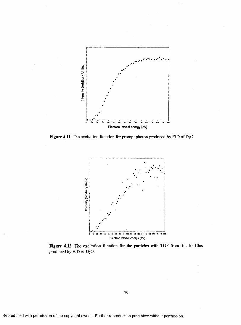
I> 10 20 30 <0 SO 60 70 W 90 100 110 100 130 140 150

Electron Impact energy (eV)

Figure 4.11. The excitation function for prompt photon produced by EID of D2O.

0 10 30 30 40 50 60 70 80 *0 100 1 10 120 130 140 1» 140 170 190 140 200

E lectron Im pact energy (eV)

Figure 4.12. The excitation function for the particles with TOF from 5us to lOus produced by EID of D2O.

70


fragment signal. In this procedure, the excitation function for the prompt photon was

used as reference since the prompt photon peak in any TOF spectrum is clear and pure.

Firstly, a set of TOF spectra corresponding to a set of different electron impact

energies had to be acquired under the same condition as when the photon excitation

function was measured. Secondly, the TOF distributions for pure fragment at different

electron impact energies were distilled from each original TOF spectrum by

subtraction of the exponential fitting curves of the decrease slope of the photon peaks

just as we have seen in last section. If it is assumed that the intensity of photon signal

is related to the intensity of each fragment signal linearly in the TOF spectrum, then

the excitation function of the pure fragment signal can be estimated on the basis of the

excitation function of prompt photon. Finally, we scaled the photon signal intensity in

each impact energy TOF data suitably so that its value matches the value of photon

excitation function at the same energy, and then adjust the fragment signal intensity in

proportion. The result turns out to be the value of the pure fragment excitation

function at the corresponding energy. A set of these discrete values represents the

tendency of the excitation function. Since this method needs to acquire TOF spectrum

at each of chosen electron energies and analyze these TOF data one by one manually,

it is impossible to sweep 1 0 0 different electron impact energies like program

controlled photon counter (SR400) does. To avoid much more calculation we only

picked up a few impact energies to analyze corresponding TOF data, however this

leaded to an excitation function with poor accuracy. The Figure 4.13 exhibits that

71


excitation function of pure fragments arriving at detector between 5us to lOus

constructed by this manual procedure. The curves between known data points were

constructed by using interpolation process. Since the increments of chosen energies

were relatively small at low energy region, the low energy data were fitted using a

shape-preserving (Piecewise cubic Hermite interpolation, PCHIP) interpolation,

which preserved monotonicity and the shape of the data. At high energy region, cubic

spline interpolation was employed for the data with relatively large energy increment.

During the fitting process, three unreliable data were excluded.

Because the electron energy spread due to the voltage drop across the filament

is about 2eV and the electron energy spread due to thermionic emission from filament

surface is about 2eV(see Chapter 3), the electron energy scale is uncertain by about

± 2eV. Another considerable aspect for the uncertainty of the threshold is the

increment of the swept energies for getting excitation function. Although

extrapolation of the fitting curve to zero can evaluates the threshold, the result is just

an approximate value. It is difficult to locate the threshold exactly in the region

between the energy settings above and below a threshold. Thus, the uncertainty can be

taken as the half of the division of two successive energy settings between which the

threshold falls. Until now, we have talked about two kinds of uncertainty among

which the larger one can be taken as the final error of the threshold.

It has been mentioned in previous chapter that an excitation function

sometimes does not change smoothly, but shows sharp turns (breaks) at some voltages.

Each of these breaks corresponds to a threshold for an individual dissociation process.

72


It is evident from Figure 4.13 that there are two breaks in the excitation function curve.

Straight-line approximation was used to the first two dots and the energy intercept of

this line is treated as the first threshold. The curve rises from zero at the first threshold

near 12.5eV to a broad peak around 115.5eV and then falls slowly. The gradual onset

is followed by two breaks that occur at approximately 23eV and 58eV respectively.

Two obvious breaks indicate that there are at least three dissociation processes

contributing to the major peak in D2O TOF spectra, which agrees with the result from

the resolution of D2O TOF spectra.

e3

inc

16

- t -12

10

—

4

12.62

050 100 150

Electron Impact Energy (eV)200 250

Figure 4.13. The excitation function for the pure fragment due to dissociation of D2O with TOF from 5us to lOus.

73


The major features of TOF spectra in Figure 4.3 are extracted in order to

eliminate the effect of prompt photon and depicted in Figure 4.8. Furthermore, this

major feature was resolved into three Gaussian-like structures by using curve fitting

process. Figure 4.8 illustrates that the third Gaussian peak is not observable in the

38eV TOF spectrum, which indicates that the threshold at about 58eV corresponds to

the dissociation process dominant in the third Gaussian structure. At 38eV incident

energy the maximum of the second Gaussian peak is two and half times greater than

that of the first Gaussian peak. Therefore, it is reasonable to assume the dominant

process for the second Gaussian structure has the threshold at about 12.5eV and the

dominant process for the first Gaussian structure has the threshold at about 23eV.

According to isotopic analysis, it has been known that only the ionic or the

neutral metastable fragments (atom or molecule), which only contain hydrogen

element, can be responsible for that major feature in Figure 4.3. If we assume the

second Gaussian structure is due to the ionic or the metastable hydrogen atom, the

released kinetic energy corresponding to that peak is 5.18eV. The dissociation limit is

given by subtraction of the released kinetic energy from the threshold. The threshold

observed in Figure 4.13 is 12.5 ± 2eV, which is close to the onset of 11 ± 2eV for the

electron impact dissociation of water measured by Freund [27]. So, the dissociation

limit for the process is calculated to be about 7.32 + 2eV.

The electron attachment during the dissociation process of the heavy water can

give rise to the formation of negative ions. H~{D~) has been shown by

74


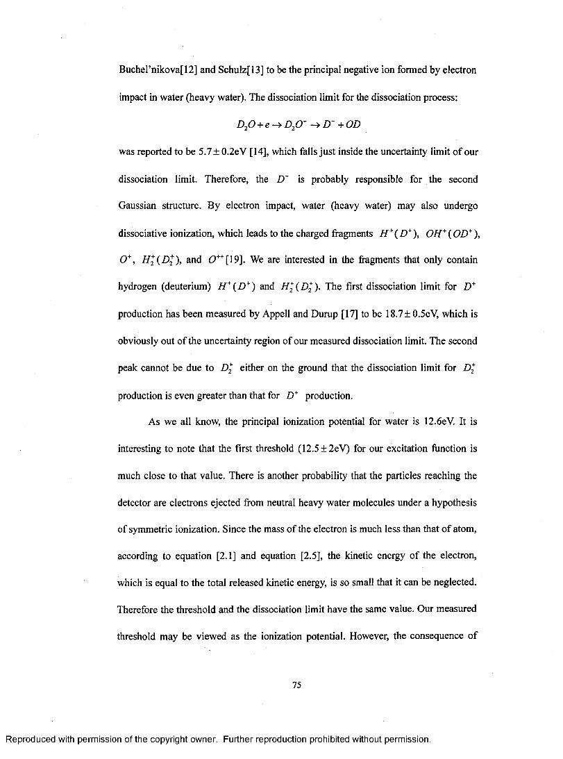
BucheFnikova[12] and Schulz[13] to be the principal negative ion formed by electron

impact in water (heavy water). The dissociation limit for the dissociation process:

DjO + c —> DjO —̂ D + OD

was reported to be 5.7± 0.2eV [14], which falls just inside the uncertainty limit of our

dissociation limit. Therefore, the D~ is probably responsible for the second

Gaussian structure. By electron impact, water (heavy water) may also undergo

dissociative ionization, which leads to the charged fragments H + ( D+), OH+ ( OD+),

0 +, ( £>2 ), and 0 ++[ 19]. We are interested in the fragments that only contain

hydrogen (deuterium) H +(D +) and H \(D *). The first dissociation limit for D +

production has been measured by Appell and Dump [17] to be 18.7+ 0.5eV, which is

obviously out of the uncertainty region of our measured dissociation limit. The second

peak cannot be due to D\ either on the ground that the dissociation limit for D\

production is even greater than that for D+ production.

As we all know, the principal ionization potential for water is 12.6eV. It is

interesting to note that the first threshold (12.5 ±2eV) for our excitation function is

much close to that value. There is another probability that the particles reaching the

detector are electrons ejected from neutral heavy water molecules under a hypothesis

of symmetric ionization. Since the mass of the electron is much less than that of atom,

according to equation [2.1] and equation [2.5], the kinetic energy of the electron,

which is equal to the total released kinetic energy, is so small that it can be neglected.

Therefore the threshold and the dissociation limit have the same value. Our measured

threshold may be viewed as the ionization potential. However, the consequence of

75


light mass of the electron is that the electron should be dissociated from the neutral

molecule with relative high velocity. From previous analysis, we know the first

threshold corresponds to the second Gaussian peak in TOF data. The velocity related

to that peak seems not to be high enough and thereby the first threshold is unlikely to

associate with a process of ionization of heavy water.

Another possible particle that is responsible to the TOF structure is the

metastable hydrogen (deuterium) atom H(2s) (D(2s)). The first threshold at about

12.5eV probably corresponds to a D(2s) dissociation process described by Freund

[27]. In this process, the heavy water is first dissociated into the ground states of D

and OD, and then D atom is excited to the metastable state of 2s, which is expressed

as:

D20 + e —> D(ls) + OD(X2H) -> D(2s) + OD(X2U)

The threshold for overall process is at 10.2eV, which is just a little bit less than lower

uncertainty limit of our first threshold (12.5 ± 2eV).

The second threshold appears at 23 ± 2eV. The most possible structure in TOF

data corresponding to this threshold is the first fitting Gaussian peak in Figure 4.8 (see

previous discussion), which is correlated with the released kinetic energy of 11.57eV

under the assumption that the peak is due to the fragment containing only one

deuterium atom. If the observed fragment was the ionic or the metastable deuterium

molecule, the released kinetic distribution mapped from that TOF data would peak at

about 26eV. Since this is greater than our threshold, the production of deuterium

molecule is clearly impossible. From the known threshold and the released kinetic

76


energy, the dissociation limit for the formation of deuterium atom was calculated to be

11.43±2eV. Dissociation to D(2s) + OD(X2JJ) has the dissociation limit at 15.3eV,

which is just outside the rather large uncertainty.

There is an indication in Figure 4.13 that, in the vicinity of a relative high

energy of 58eV, a new dissociation channel opens. The process that is identified to

correspond to this threshold is the third Gaussian peak in TOF spectrum (Figure 4.8).

If it is assumed that one-deuterium-containing fragment is responsible for the peak,

the correlated released kinetic energy is obtained to be about 3.69eV, which is very

close to the kinetic energy of 3.7eV for metastable H(2s) reported by Clampitt [26].

However, there appears to be significant disagreement with the results of Clampitt.

Our measured threshold is much larger than his reported threshold of 19eV for

H(2s)+OH. We cannot presently determine this observed particle just on base of our

data. It must be checked by further experiment.

Conclusions

Time-of-Flight spectroscopy was used to study the fragmentation of H2O and

D2O following electron impact. By comparison between TOF spectra from H20 and

D2O, isotopic shifts were observed. Under the hypothesis of two-body dissociation or

symmetric three-body dissociation, substitution of deuterium for hydrogen can make

peaks in TOF data due to oxygen-containing fragments shift to shorter flight times

and peaks due to fragments only containing deuterium element shift to longer flight

time. By analysis o f isotopic shifts, the major peak in our TOF spectrum was

77


determined to correspond to the fragments only containing hydrogen. In addition,

deconvolution of the major peak into three separate Gaussian-like structures has been

illustrated.

The excitation function related to the major peak in D20 TOF data has been

studied over the range from OeV to 300eV. At least three different production

mechanisms have been identified. The onset energy was found to be 12.5±2eV, which

agreed with the work of Freund. The possible dissociation processes for this threshold

are:

DjO + c —> DjO —i D + OD

or

D20 + e^> D(ls) + OD(X2U) D(2s) + OD(X2II)

Further research is required to determine which one is the right one.

The second threshold occurred at 23±2eV. If the detected fragment was

production of deuterium atom, the dissociation limit turned out to be 11.43±2eV,

which was close to the dissociation limit (15.3eV) of the process:

D20 -^D (2 s ) + 0D (X2n )

The third threshold was found to be about 58eV. This threshold probably was

due to high Redberg state of deuterium, which must be check by further experiment.

78


Chapter 5

H20 2 Results

Figure 5.1 shows several time-of-flight distributions yield at different electron

impact energies by using hydrogen peroxide as target. All spectra in this figure were

due to the fragments following a 2.5us pulsed electron beam, which maintains a

period of lOOOus. The electron current collected at Faraday cup was kept about 0.3uA

for the impact energy from 18eV to 300eV. At each impact energy the experiment has

been running as long as others to obtain TOF data. The head pressure of the target

vapor was fixed approximately 2.5torr. But, it should be noted that our source used for

evaporation is actually a concentration of 30% aqueous solution of H20 2. The solution,

therefore, raised a mixture of water and hydrogen peroxide vapor. Fortunately,

Raoult’s Law is a possible way of obtaining equilibrium vapor pressures of the

components of an ideal solution. This allowed us to estimate the head pressures of

H20 and H20 2. The ratio of pressure of H20 2 to pressure of H20 was about 0.009 for

concentration 30% aqueous solution of H20 2 at temperature of 28°C (see Appendix

for detail of calculation). That meant the water content was the dominant component

of the gas mixture. Relative low pressure of H20 2 brought the trouble that the signal

of H20 2 was very weak relative to signal of H20 produced simultaneously.

79


600

500

-4-JcD£12

1

400

138eV

300

< 38eV

j|2 200 « 23eV

100

13eV

160 180 200120 1400 100

Time (us)

Figure 5.1 TOF spectra for H2O2 at electron impact energies shown in diagram.

80


For the convenience of viewing the signal, the TOF curves are all displaced

upward except for the 18eV data. The signal at very short times is due to the prompt

photons that are produced by decay of excited particles when electron pulse is

activated. The center of this prompt photon peak is taken as the zero o f the time scale.

Figure 5.1 illustrates that the pattern and intensity of the TOF signal varies

significantly over our studied impact energy range. At energy of 13eV the primary

feature of the TOF spectra is the peak at approximately 95us. This feature appears to

decrease with increase of the impact energy. It only contributes as a shoulder at

energy of 38eV, and it is barely visible at energies greater than 138eV. In 23eV energy

TOF data a new structure is observed as a broad peak at around 45us. In contrast to

the peak near 95us, this feature grows up with increase of impact energy until the

energy of 138eV at which it is most intense. The TOF data also demonstrate that the

fastest peak at about 6 us, which is not present at impact energies of 23eV and 13eV,

becomes apparent at higher impact energies. The maxima of all peaks do not appear to

obviously shift in time with increase of impact energy. Since peaks appear or

disappear with change of energy and their heights alter with energy, it is probable that

more than one dissociation process are contributing to the TOF signal. Moreover,

there exist the competition between these processes, and different process plays

dominant role by turns at different impact energies.

81


1700

1600 -

1500 -

1400 -

V 1 3 0 0 -

■ £ 1200 -

1100 -

g 1000 -

I 900 -< 800 -

> 700

600

500 -

400 -

300 -

200 -

100 -

140 18016012060 80 10040200

Time (us)Figure 5.2 Comparison of TOF spectra for H20 , H20 2, and 0 2 at impact energy of lOOeV.

82


The feature that takes place at around 6 us looks familiar. It reminds us the

TOF data of water (Figure 4.1) in which a peak appears almost at the same time. The

peak at approximately 45us is very similar as the feature occurs in TOF of oxygen

molecule. For convenience of comparison, we plotted the TOF data of H2O, H2O2,

and O2 at impact energy of lOOeV on one time scale as shown in Figure 5.2. All TOF

spectra were obtained during the time interval with the same length and under

identical conditions. It is clear that, at lOOeV energy, the TOF data of H2O2 is actually

the mixture of TOF data of H2O and TOF data of O2 . It is not a surprise that the

features of FfeO appear in TOF data of H2O2 . We have discussed above that the water

content is much more than hydrogen peroxide content in vapor mixture evaporate

from concentration 30% aqueous solution of H2O2. By comparing with TOF spectrum

of O2, the peak occurred at around 45us is obviously due to the dissociation of oxygen

molecule. A possible interpretation for the source of oxygen molecule is the

decomposition of the hydrogen peroxide:

2H20 2 —> 2H20 + 0 2.

Even though part of H2O2 decomposes into O2, the signal due to O2 should not

be strong since the H2O2 content is rare in vapor mixture. If we assume the intensity

of the signal is proportional to the pressure of the target gas, which is linear with the

gas concentration for ideal gas. Figure 5.2 illustrates that the intensity of peak at 45us

for H2O2 is a quarter of the intensity of the peak at same time for O2 . That indicates

the pressure of the O2 is about one fourth of the total pressure, which is much greater

the ratio of H2O2 vapor pressure to the total vapor pressure because of evaporation

83


- 4 - - 4 -

-----f h f — 4 - -I------

--------\ -H ------- + - - d —I

I +- t f i f - + -----€&£m

f - —— t \ - t —IH202 l

4— 1------C

~ \------------ f 1—

8 12 280 4 16 20E lectron Im pact E n erg y (eV)

Figure 5.3 Excitation functions for fragmentation of oxygen and hydrogen peroxide produced by EID.

84


(see Appendix). There must be other sources providing the oxygen molecules.

Oxygen impurity in the pipes due to uncompleted pumping may be a possible

explanation of the extra source of the oxygen molecule.

Now, let us give some attention to the TOF spectra at low impact energy in

Figure 5.1. The peak at around 95us, which appears as a shoulder in TOF data of O2 at

energy of lOOeV, is the only feature at the lowest impact energy. Figure 5.2

demonstrates that our target gas is a mixture of H2O vapor and O2 gas. At low

energies the features of H2O do not appear, which means the dissociation of O2 is the

dominant process. Furthermore, the threshold of our experiment is supposed to be

same as that of process of dissociation of O2. Figure 5.3 shows the excitation function

curves of 0 2 and H2O2 together in one diagram. All possible TOF signals are involved

in to obtain the excitation functions in this figure. It is clear that the onsets of two

curves are very close: the threshold for signal from O2 is at about 7.9eV; the threshold

for signals from H2O2 is at about 8.2eV. This is the further proof of our earlier

conclusion. If the particle responsible to the peak at 96us is assumed to be the

metastable oxygen 0 (5S), the corresponding kinetic energy is about 0.63eV. By using

two-body dissociation model, the total released kinetic energy is calculated to be

1.26eV, and then the dissociation limit is obtained as 6.94eV. We cannot presently

identify the dissociation process occurred in our experiment. A more conclusive

interpretation of H2O2 dissociation requires further research.

85


Chapter 6

Suggestion for future study

The analysis of our experimental results (TOF spectra, and excitation function)

can be preformed only if the type, mass, and quantum state of the detected fragment

can be identified. In actuality, it is not effective to identify the fragments fling away

from the parent molecule only by using our detector, channeltron, because of the fact

that channeltron is sensitive not only to the metastables of H(2s) and 0 (5S) but also to

photons, ions and some high energy Rydberg states. The usual way of distinguishing

the H(2s) signal from others is to introduce quenching electric field. In the electric

field, the mixture of the state 2s and 2p takes place so that the number of the H(2s) in

the beam is reduced, which is accompanied by photon emission. Although two

grids ,between which electric field can be formed, are mounted in front of the

channeltron, they are so close to the detector that the surface of detector still cover

relative large solid angle with respect to the center of the electric field. Since the

photon emission due to quenching effect is supposed to be spherical symmetry,

relative large solid angle of detector surface cause sufficient photons, which

correspond to the metastable H(2s), to be captured by detector. By comparing with the

signals with quenching field off, the signal of H(2s) cannot be removed completely by

quenching field. Therefore, we suggest placing a pair of extra plates far away from the

channeltron, which can form a weak electron field perpendicular to the line of sight.

86


This field combining the field right before the detector can help us identify the

negative ion, positive ion, and metastable H(2s).

In chapter 4, much effort was made to remove the effect of the long tail of

prompt photon signal and to distinguish a signal corresponding to a dissociation

process from a convolved signal. Moreover, since signals for different fragments have

merged together, it is impossible to obtain an excitation function for a unique

fragment directly. We have to estimate the excitation function from TOF spectra. The

complicated calculation limits the number of the TOF spectra involved in this

estimation so that the accuracy of the estimated excitation function is low. One

possible solution of improving the resolution of each fragment signal is to narrow the

width of the electron pulse. Shorter electron pulse can restrain the spread of the TOF

spectra and thereby result in relative sharp fragment peaks. Short electron pulse has

another advantage of reducing the error in RKE corresponding to short flight time as

discussed in chapter2 and chapter 4. Thus, in the future, it is desired that the electron

pulse control could be modified to produce shorter pulse. As consequence of this

modification, the effect of long photon decay tail on the signal with short TOF could

be attenuated and the fragment signals, which used to be mixed, may distinguish

themselves from others. Additionally, the accuracy of RKE data could be improved,

especially for that corresponding to short flight time.

Analyses of the results of H2O2 demonstrated that our attempt of investigating

the electron impact dissociation process of H2O2 failed. The reason is that relative low

concentration (30%) water solution of H2O2 was used as the source of vapor. Vapor

87


pressure of H2O2 is much lower than that of H2O so that the signal from dissociation

of H2O2 is too weak to be detected. In addition, we found the signal of the O2

dissociation, which indicates that the spontaneous decomposition may occur during

the experiment. We suggest using high concentration solution to repeat this

experiment, and substituting glass made pipes for stainless steel made pipes in order

to lower the probability of spontaneous decomposition.

88


References

[1]. D.A. Vroom and FJ. de Heer, J. Chem. Phys. 50,1883 (1969).

[2]. N. Bose and W. Sroka, Z. Naturforsch. 28a, 22 (1973).

[3]. C.I.M. Beenakker, FJ. de Heer, H.B. Krop, and GR. Mohlmann, Chem. Phys. 6 ,

445 (1974).

[4], N. Kouchi, K. Ito, Y. Hatano, N. Oda, and T. Tsuboi, Chem. Phys. 36, 239 (1979).

[5]. T. Ogawa, N. Yonekura, M. Tsukada, S. Ihara, T. Yasuda, H. Tomura, K.

Nakashima, and H. Kawazumi, J. Phys. Chem. 95, 2788 (1991).

[6 ]. C.M. Lawrence, Phys. Rev. A2, 397 (1970).

[7]. C. Hayakawa, Proc. Phys. Math. Soc. Japan. 26, 78 (1944).

[8 ]. S. Tsurubuchi, T. Iwai and T. Horie, J. Phys. Soc. Japan. 36, 537 (1974).

[9]. H. Kawazumi, and T. Ogawa, Chem. Phys. 114, 149 (1987).

[10]. M. Darrach and J.W. McConkey, Chem. Phys. Lett. 184,141 (1991).

[11]. T. Harb, W. Kedzierski, and W. McConkey, J. Chem. Phys. 115, 5507 (2001).

[12]. I.S. Buchel’nikova, Zh. Eksperim. i Teor. Fiz. 35, 1119 (1958). [English transl.:

Soviet Phys.—JETP. 8 , 783 (1959)].

[13], GJ. Schulz, J. Chem. Phys. 33, 1661 (1960).

[14]. R.N. Compton, and L.G Christophorou, Phys. Rev. 154, 110 (1967).

[15]. J. Schutten, F.J. de Heer, H.R. Moustafa, A.J.H. Boerboon, and J. Kistemaker, J.

Chem. Phys. 44, 3924 (1966).

[16]. H. Ehrhardt, and A. Kresling, Z. Naturf. 22a, 2036 (1967).

89


[17]. J. Appell, and J. Durup, Int. J. Mass Spectrom. Ion Phys. 10, 247 (1972/73).

[18]. R.B. Cordaro, K.C. Hsieh, and L.C. McIntyre Jr, J. Phys. B: At. Mol. Phys. 19,

1863 (1986).

[19]. J.J. Olivero, R.W. Stagat and A.E.S. Green, J. Geophys. Res. 27, 4797 (1972).

[20]. S. Trajmar, D.F. Register and A. Chutjian, Phys. Rep 97, 219 (1983).

[21]. K.Niira, J. Phys. Soc. Japan. 4, 230 (1949).

[22]. K.Niira, J. Phys. Soc. Japan. 7, 193 (1952).

[23]. K.J. Laidler, J. Chem. Phys. 22, 1740 (1954).

[24]. J.C. Leclerc, J.A. Horsley, and J.C. Lorquet, Chem. Phys. 4, 337 (1974).

[25]. C.R. Claydon, GA. Segal, and H.S. Taylor, J. Chem. Phys. 54, 3799 (1971).

[26]. R. Clampitt, Phys. Lett. 28A, 581 (1969).

[27], R.S. Freund, Chem. Phys. Lett. 9, 135 (1971).

[28].W. Kedzierski, J. Derbyshire, C. Malone, and J.W. McConkey, J. Phys. B: At.

Mol. Opt. Phys. 31, 5361 (1998).

[29]. G. Allcock and J.W. McConkey, Chem. Phys. 34, 169 (1978).

[30]. H. Bethe, Ann. Physik 5,325 (1930).

[31]. M. Inokuti, Rev. Mod. Phys. 43, 297 (1971).

[32]. U. Fano, Phys. Rev. 95, 1198 (1954).

[33]. V.I. Ochkur, Soviet Phys. J.E.T.P. 18, 503 (1964).

[34]. I.D. Latimer and J.W. McConkey, Proc. Phys. Soc. 8 6 , 745 (1965).

[35]. L.R. LeClair, “Production and Detection of Metastable Atomic Oxygen”. Ph.D.

thesis, University of Windsor (1993), Chapter 3.

90


[36]. S. Trajmar and J.W. McConkey, “Adv. At. Mol. Opt. Phys.” Ed M Inokuti,

Academic Press, NY (1993).

[37]. E.C. Zipf, Electron-Molecule Interaction and their Application 1, Academic

Press, NY (1984).

[38]. N.J. Mason and W.R. Newell, J. Phys. B22,2297 (1989).

[39]. C.P. Malone, ‘Electron-cluster Interaction: Excitation of Neutral Fragment in

Rare Gas and Simple Molecules” PhD thesis. University of Windsor (2003).

[40]. M. Misakian, M.J. Mumma, and J.F. Faris, J. Chem. Phys. 62, 3442 (1975).

[41]. J.J. Corr, M.Sc. Thesis, University of Windsor (1987).

[42]. J.M. Ajello, et al. Appl. Opt. 27, 890 (1988).

[43]. L.R. LeClair, “Production and Detection of Metastable Atomic Oxygen”. Ph.D.

thesis, University of Windsor (1993), Chapter 4.

[44]. F.H. Field and J.L. Franklin, “Electron Impact Phenomena”, Academic Press,

NY (1970).

[45]. Karras, William Leslie, thesis, University of Windsor (1988).

[46]. D.W.O. Heddle, Proc. Phys. Soc. London 90, 81 (1967).

91


Appendix

The relationship between saturated H2O2 and H2O vapor

The purpose of this appendix is to generalize the method reviewed by Schumb

[A-l] for calculating equilibrium vapor pressure and composition of hydrogen

peroxide-water mixture.

Let us firstly consider the situation of pure substance. The saturated water

vapor pressure given by Keyes [A-2] can be expressed in denary logarithm form as

log10 (T) = G + A /T + B\ogl0 T + CT + D T2+ ET3 + F T 4 [A-q-1]

where T is the absolute temperature, A=-2892.3693, B=-2.892736, C=-4.9369728e-3,

D=5.606905e-6, E=-4.645869e-9, F=3.7874e-12, and G=19.3011421. For the

saturated vapor pressure of H2O2, the similar expression was derived by Scatchard et

al [A-3]. That is,

logio Ph (T) = D + A IT + B log10 T + CT [A-q-2]

where A, B, C, and D are constants, A=-4025.3, B=-12.996, C=4.6055e-3, and

D=44.5706.

For the situation of solution made up of volatile materials, Raoult’s law is

helpful to find the vapor pressure of components to the composition of the solution.

The law states that the vapor pressure of each component is proportional to its mole

fraction, and the proportionality constant is simply the vapor pressure of the pure

92


component. In mathematical form, it is expressed as

P,=P,0xi [A-q-3]

where Pj is the vapor pressure of component i , P® is the vapor pressure of componet i

when it is pure, Xj is the mole fraction of component i in the solution. Unfortunately,

because of the bond formed between H2O2 and H2O molecules, Raoult’s law cannot

be directly used for aqueous solution of hydrogen peroxide. An activity coefficient, n,

has to be introduced to modify the equation [A-q-3]:

P,=P°x,r, [A-q-4]

Scatchard et al calculated the activity coefficients for water and hydrogen

peroxide [A-3]. They are given by

=exP{ ^ ^ - [ 5 0 + -5, (1 - 4xw ) + B2( \ - 2xw )(1 - 6xw)]} [A-q-5]

and

rh =exp { ^ [ B 0 +Bl(3 -4 x w) + B2( l - 2 x w)(5 -6xw)]} [A-q-6 ]

where the subscripts w and h refer to water and hydrogen peroxide respectively. xw is

the mole fraction water in solution, R is the universal gas constant. Bo=-1017+0.97T,

Bi=85, and B2=13. The equation [A-q-5] actually involves the fact that the sum of the

mole fraction of the components in solution must be unity, xh + xw = 1. If we assume

the vapors are ideal gases, according to Dalton’s law, the total vapor pressure above

the solution is equal to the sum of the vapor pressure of components, Plol =Ph +Pw.

The vapor pressure we are talking about is the pressure of vapor in equilibrium

with the liquid. It is not the head pressure we measured in experiment. Ejection of

93


target gas through capillary could be treated as the process of throttle. The relative

high vapor pressure in source container is reduced to relative low head pressure by

throttle. In the case of gas mixture, the ratio of pressure of components before the

throttle is supposed to be same as that after the throttle under the assumption of ideal

gases.

In this work we used the H2O2 solution with a concentration of 30%, which

can be translated to the mole fraction of about 0.18. If the room temperature of 28°C

is taken as T to feed into above equations, the pressures of H2O2 and H2O, and the

ratio of them can be calculated. The results are shown as follow.

Pw *21.92 torr

Ph «0.19 torr

« 0.009.P.

References

A-l. W.C. Scumb et al., Amer. Chem. Soc. Monograph (1955).

A-2. F.GKeyes, J. Chem. Phys. 15, 602 (1947).

A-3. GScatchard et al., J. Am. Chem. Soc. 74, 3715 (1952).

94


Vita Auctoris

NAME:

PLACE OF BIRTH:

YEAR OF BIRTH:

EDUCATION:

Xinqing Liao

Beijing, China

1976

The High School attached to Tsinghua UniversityBeijing, China1991-1994

Shanghai Jiaotong University Shanghai, China 1994-1998

University of Windsor Windsor, Ontario, Canada 2003-2006

95


Metastable production from electron impact dissociation of ...

Documents

Transcript of Metastable production from electron impact dissociation of ...