METHODOLOGY Open Access

Metabolite AutoPlotter - an application toprocess and visualise metabolite data inthe web browserMatthias Pietzke1* and Alexei Vazquez1,2

Abstract

Background: Metabolomics is gaining popularity as a standard tool for the investigation of biological systems. Yet,parsing metabolomics data in the absence of in-house computational scientists can be overwhelming and time-consuming. As a consequence of manual data processing, the results are often not analysed in full depth, sopotential novel findings might get lost.

Methods: To tackle this problem, we developed Metabolite AutoPlotter, a tool to process and visualise quantifiedmetabolite data. Other than with bulk data visualisations, such as heat maps, the aim of the tool is to generatesingle plots for each metabolite. For this purpose, it reads as input pre-processed metabolite-intensity tables andaccepts different experimental designs, with respect to the number of metabolites, conditions and replicates. Thecode was written in the R-scripting language and wrapped into a shiny application that can be run online in a webbrowser on https://mpietzke.shinyapps.io/autoplotter.

Results: We demonstrate the main features and the ease of use with two different metabolite datasets, for quantitativeexperiments and for stable isotope tracing experiments. We show how the plots generated by the tool can be interactivelymodified with respect to plot type, colours, text labels and the shown statistics. We also demonstrate the applicationtowards 13C-tracing experiments and the seamless integration of natural abundance correction, which facilitates the betterinterpretation of stable isotope tracing experiments. The output of the tool is a zip-file containing one single plot for eachmetabolite as well as restructured tables that can be used for further analysis.

Conclusion:With the help of Metabolite AutoPlotter, it is now possible to simplify data processing and visualisation for awide audience. High-quality plots from complex data can be generated in a short time by pressing a few buttons. This offersdramatic improvements over manual analysis. It is significantly faster and allows researchers to spend more time interpretingthe results or to perform follow-up experiments. Further, this eliminates potential copy-and-paste errors or tedious repetitionswhen things need to be changed. We are sure that this tool will help to improve and speed up scientific discoveries.

Keywords: Metabolites, Metabolomics, Processing, Visualisation, Graphs, Plots, Automatic

© The Author(s). 2020 Open Access This article is licensed under a Creative Commons Attribution 4.0 International License,which permits use, sharing, adaptation, distribution and reproduction in any medium or format, as long as you giveappropriate credit to the original author(s) and the source, provide a link to the Creative Commons licence, and indicate ifchanges were made. The images or other third party material in this article are included in the article's Creative Commonslicence, unless indicated otherwise in a credit line to the material. If material is not included in the article's Creative Commonslicence and your intended use is not permitted by statutory regulation or exceeds the permitted use, you will need to obtainpermission directly from the copyright holder. To view a copy of this licence, visit http://creativecommons.org/licenses/by/4.0/.The Creative Commons Public Domain Dedication waiver (http://creativecommons.org/publicdomain/zero/1.0/) applies to thedata made available in this article, unless otherwise stated in a credit line to the data.

* Correspondence: matthias.pietzke@gmail.com1Cancer Research UK Beatson Institute, Switchback Road, Bearsden, GlasgowG61 1BD, UKFull list of author information is available at the end of the article

Pietzke and Vazquez Cancer & Metabolism (2020) 8:15 https://doi.org/10.1186/s40170-020-00220-x

BackgroundData analysis for metabolomics can typically be sepa-rated into two parts. In the first part, often termed aspre-processing, the raw measurements are convertedinto readouts. This includes reading the mass-spectrometer raw files, peak detection and integration,metabolite identification and alignment of metabolitesover several measurements [1, 2]. In the second part ofthe analysis, researchers need to convert readouts intobiological insights. While there are tools to carry on theidentification and quantification of metabolites [3], weare still missing user-friendly interfaces to perform sta-tistics and visualise the data. These tasks typically in-clude the association of measurements to conditions,grouping and averaging of replicate measurements, cor-rection of the intensities by cell counts or internal stan-dards and finally visualising the results.It is difficult to define a universal solution due to dif-

ferent data structures generated with different analytictools, different experimental setups and finally differentpersonal visual preferences. As a consequence, we foundothers and ourselves repeating similar steps manuallyover and over again, extracting data for selected metabo-lites to be imported in graphic tools such as GraphPadPrism or plotting metabolite intensities with MicrosoftExcel. However, manual data processing is extremelytime-consuming and prone to errors.To automate these steps, we developed Metabolite

AutoPlotter, a web-based application for the analysis ofmetabolomics data, conveniently automatizing the stepsin metabolomics data processing, leading to well-structured tables and graph outputs for every metabolitein the dataset. The graphs can be customised with re-gard to plot type, colours, text labels and size amongother features. Additionally, statistical tests can be con-ducted and the results added to the graphs. The mostimportant features are described in detail in the follow-ing sections.

MethodsImplementationMetabolite AutoPlotter is written in R [4] and wrappedinto a web-application with the “shiny” package [5]. Datamanipulation is realised mainly with tools from the“tidyverse” package [6], the plotting is realised with“ggplot2” [7] and for the individual data points, “ggbees-warm” is used. For reading and writing Excel files,“readxl” and “writexl” are used; for creating the reportfile, we use “officer”. Statistics is implemented with“ggpubr”, containing a wrapper for the “ggsignif” pack-age. Summary pages are created using “gridExtra”, thepalettes are used from the “pals” package and colourblind simulation is performed using “colorspace”. Theappearance of the application is improved with

“shinythemes”, “shinycssloaders”, “shinyWidgets” and“shinyalert”. For zipping of the results, the “zip” packageis used. All packages and the R-version are routinelyupdated.

Generation of metabolite data for a quantitativeexperimentFor the quantitative demo data, we extracted intracellu-lar metabolites from 5 different tissues (brain, liver, kid-ney, spleen and pancreas) from a 13C-tracing experimentwith 13C-methanol in four different mice [8]. Metaboliteextraction and LC-MS measurement were performed asdescribed in [9]. Only the unlabelled metabolites areused here, to show the differences between the tissues.Peak areas were extracted using TraceFinder-software(Thermo Fisher), by comparing the mass to charge ratio(m/z) and the retention time against a custom libraryprepared with authentic standards. The dataset contains99 metabolites measured for 3 time-points in 4 bio-logical replicates.

Generation of metabolite data for tracing experimentThis dataset was generated exclusively for the purpose ofshowing the tracing features of this tool. For this, HCT116cells were incubated for four different time points (1 h, 3h, 6 h and 24 h) in Dulbecco’s modified Eagle’s medium(DMEM) either containing u-13C6-Glucose (17mM) oru-13C5-glutamine (2 mM) in triplicate wells. Intracellularmetabolites were extracted and measured by LC-MS againas described in [9], and 38 metabolites were extractedusing TraceFinder-software (Thermo Fisher).

Implementation of default coloursAs default colours for the plots, we use the schemes de-veloped by Paul Tol (https://personal.sron.nl/~pault/)and their implementation in the pals-package. This de-livers a harmonic appearance while simultaneouslymaintaining a fair amount of separation for people withcolour-impaired vision. For quantitative experiments,the user can define its own colours in the sample tableeither in hex-notation (e.g. #FFAA25) or using the pre-defined colour names for R. For tracing experiments, thecolours are hardcoded to guarantee an identical appear-ance between experiments. Here, the user can choosebetween the short scale, a modification of the tol-rainbow, with saturation and value increased by 20%,and the long scale is based on the stepped rainbow.

ResultsData importMetabolite AutoPlotter reads quantified data containingthe identified metabolites and their intensities, generatedelsewhere, e.g. with manufacturer’s software or othersoftware tools for peak detection and metabolite

Pietzke and Vazquez Cancer & Metabolism (2020) 8:15 Page 2 of 11

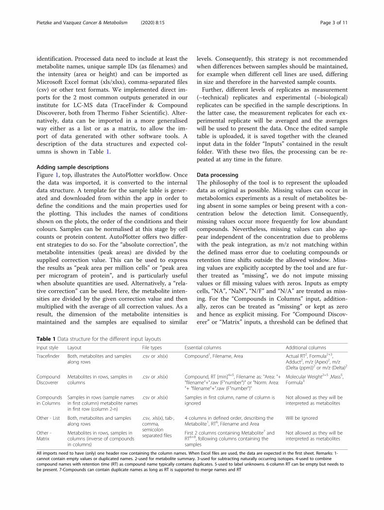
identification. Processed data need to include at least themetabolite names, unique sample IDs (as filenames) andthe intensity (area or height) and can be imported asMicrosoft Excel format (xls/xlsx), comma-separated files(csv) or other text formats. We implemented direct im-ports for the 2 most common outputs generated in ourinstitute for LC-MS data (TraceFinder & CompoundDiscoverer, both from Thermo Fisher Scientific). Alter-natively, data can be imported in a more generalisedway either as a list or as a matrix, to allow the im-port of data generated with other software tools. Adescription of the data structures and expected col-umns is shown in Table 1.

Adding sample descriptionsFigure 1, top, illustrates the AutoPlotter workflow. Oncethe data was imported, it is converted to the internaldata structure. A template for the sample table is gener-ated and downloaded from within the app in order todefine the conditions and the main properties used forthe plotting. This includes the names of conditionsshown on the plots, the order of the conditions and theircolours. Samples can be normalised at this stage by cellcounts or protein content. AutoPlotter offers two differ-ent strategies to do so. For the “absolute correction”, themetabolite intensities (peak areas) are divided by thesupplied correction value. This can be used to expressthe results as “peak area per million cells” or “peak areaper microgram of protein”, and is particularly usefulwhen absolute quantities are used. Alternatively, a “rela-tive correction” can be used. Here, the metabolite inten-sities are divided by the given correction value and thenmultiplied with the average of all correction values. As aresult, the dimension of the metabolite intensities ismaintained and the samples are equalised to similar

levels. Consequently, this strategy is not recommendedwhen differences between samples should be maintained,for example when different cell lines are used, differingin size and therefore in the harvested sample counts.Further, different levels of replicates as measurement

(~technical) replicates and experimental (~biological)replicates can be specified in the sample descriptions. Inthe latter case, the measurement replicates for each ex-perimental replicate will be averaged and the averageswill be used to present the data. Once the edited sampletable is uploaded, it is saved together with the cleanedinput data in the folder “Inputs” contained in the resultfolder. With these two files, the processing can be re-peated at any time in the future.

Data processingThe philosophy of the tool is to represent the uploadeddata as original as possible. Missing values can occur inmetabolomics experiments as a result of metabolites be-ing absent in some samples or being present with a con-centration below the detection limit. Consequently,missing values occur more frequently for low abundantcompounds. Nevertheless, missing values can also ap-pear independent of the concentration due to problemswith the peak integration, as m/z not matching withinthe defined mass error due to coeluting compounds orretention time shifts outside the allowed window. Miss-ing values are explicitly accepted by the tool and are fur-ther treated as “missing”, we do not impute missingvalues or fill missing values with zeros. Inputs as emptycells, “NA”, “NaN”, “N/F” and “N/A” are treated as miss-ing. For the “Compounds in Columns” input, addition-ally, zeros can be treated as “missing” or kept as zeroand hence as explicit missing. For “Compound Discov-erer” or “Matrix” inputs, a threshold can be defined that

Table 1 Data structure for the different input layouts

Input style Layout File types Essential columns Additional columns

Tracefinder Both, metabolites and samplesalong rows

.csv or .xls(x) Compound1, Filename, Area Actual RT2, Formula2+3,Adduct2, m/z (Apex)2, m/z(Delta (ppm))2 or m/z (Delta)2

CompoundDiscoverer

Metabolites in rows, samples incolumns

.csv or .xls(x) Compound, RT [min]4+5, Filename as: "Area: "+"filename"+".raw (F"number")" or "Norm. Area:"+ "filename"+".raw (F"number")"

Molecular Weight2+5 ,Mass5,Formula3

Compoundsin Columns

Samples in rows (sample namesin first column) metabolite namesin first row (column 2-n)

.csv or .xls(x) Samples in first column, name of column isignored

Not allowed as they will beinterpreted as metabolites

Other - List Both, metabolites and samplesalong rows

.csv, .xls(x), tab-,comma,semicolonseparated files

4 columns in defined order, describing theMetabolite1, RT6, Filename and Area

Will be ignored

Other -Matrix

Metabolites in rows, samples incolumns (inverse of compoundsin columns)

First 2 columns containing Metabolite7 andRT6+8, following columns containing thesamples

Not allowed as they will beinterpreted as metabolites

All imports need to have (only) one header row containing the column names. When Excel files are used, the data are expected in the first sheet. Remarks: 1-cannot contain empty values or duplicated names. 2-used for metabolite summary. 3-used for subtracting naturally occurring isotopes. 4-used to combinecompound names with retention time (RT) as compound name typically contains duplicates. 5-used to label unknowns. 6-column RT can be empty but needs tobe present. 7-Compounds can contain duplicate names as long as RT is supported to merge names and RT

Pietzke and Vazquez Cancer & Metabolism (2020) 8:15 Page 3 of 11

Fig. 1 The visual design of the tool. Top: Scheme illustrating the workflow of the application. Bottom: Screenshot of the application, showing theplot-design step. The plot in the middle is interactively updated based on the settings defined by the user, allowing a high level of flexibility

Pietzke and Vazquez Cancer & Metabolism (2020) 8:15 Page 4 of 11

need to be reached; below that threshold values aretreated as missing. In line with this, we do not normal-ise, scale or transform the data. Although this is requiredfor some further analysis (principal component analysis(PCA), independent component analysis (ICA), partialleast square discriminatory analysis (PLS-DA) or cluster-ing), this is not needed to show the data. The presenceof missing values helps to identify poor measurementsor noisy metabolites, while the addition of missing valueimputation may gain false confidence.At the step of data processing, metabolites can be nor-

malised with internal standards. Normalisation can beperformed before or after the external normalisation.The first case is suited for standards added during theextraction step, to compensate for variations duringsample preparation and measurement. The latter case isuseful when the intensities should be normalised to adetected metabolite. Similar to the external normalisa-tion values can be normalised absolutely or relatively.Multiple metabolites can be selected and will besummed up, consequently, the normalisation is more af-fected by highly abundant metabolites. When there isnot a single metabolite serving as a representative forthe other compounds, samples can additionally be nor-malised with the sum of all peak areas (“Total PeakSum”).To further evaluate the quality of the data, we also in-

clude a quality control feature to evaluate the perform-ance of the replicate measurements. For this, the relativefold changes for each metabolite between the replicatesof the same condition are calculated and shown for allmetabolites together. The means of all the metabolitesshould be centred around 1 when the replicates performcomparably. This strategy evaluates the quality of thesamples based on all detected metabolites, is independ-ent of outliers in single metabolites and missing valuesand works well for a small number of replicates. Samplesthat differ dramatically at this stage can be identifiedand removed conveniently before performing furtheranalysis.After the data are processed, structured tables are

exported together with the plots. These tables can beused for further processing, statistical analysis or to im-port the data into other visualisation tools, e.g. Graph-Pad Prism. A detailed explanation of the exports isincluded in Supplement File 1, and is exported togetherwith the results.

Application to quantitative experimentsThe most important and unique feature of the tool is toautomatically generate one single graph for every com-pound in the dataset. As this highly depends on the userpreferences, we included an interface that allows an

interactive customisation of the plot design (Fig. 1,bottom).Four different plot types are currently included in the

application: bar plot, violin plot, box plot, and univariatescatterplots (Fig. 2a–c and e). The bar plots show themean and the standard deviation, the same applies tothe scatterplots that additionally show the individualmeasurements. The violin plots show the density distri-bution and the median, the box plots show the median,the 25th and 75th percentiles and the lowest/highestvalue within 1.5 times inter-quartile range from the box.Violin plots and box plots only make sense when enoughdata points are present, so they are only available when5, respectively 10 replicate measurements per condition,are present in the dataset. When technical and experi-mental replicates are present, the user can additionallygenerate 2 different plots that allow for the comparisonof the performance within the replicates (Fig. 2d, f).

Plot personalisationAll plots can be further modified beyond the default set-tings (Fig. 2g–k). Already with the sample descriptions,the order of the conditions and their colours can be de-fined (Fig. 2, right vs. Fig. 2, left). Bar, box and violinplots can be generated with outlined colour instead offilled colour to reduce their weight and amount of inkused (Fig. 2h, i). Additionally, the individual data pointscan be overlaid over each of the plots (Fig. 2h). Further-more, the dimensions of the plots (width and height),their resolution and the output format (jpg, pdf, png,svg) can be defined. Also, the text elements can be al-tered, this includes the sizes, the direction of the textalong the x-axis, the axis titles for x- and y-axes. Add-itional text can be added on the left or the right side ofthe compound names to add some experimental descrip-tions. Simple statistics can be added as well; this can beeither multiple pairwise comparisons or comparisonsagainst one reference group, as t test (expecting equalvariances) or Wilcoxon test. The results of the statisticscan be shown as symbols or numeric values (Fig. 2i, j).Once the design is defined, the user can click on “Gen-

erate all plots!” and a plot for every metabolite is savedas an image file with the metabolite name as the file-name. Characters not allowed in filenames (e.g. :, ;, <, >)are converted automatically during this step. All results(the plots and the tables) are packed into a zip file thatcan be downloaded by the user.Bar plots belong to the standard repertoire for data

visualisation, as they are easily understood by anyoneand can be effectively used to screen for differences dueto the weight of the different colours. However, we wantto point out that they are probably not the best repre-sentation in all cases. First of all, the data usually do notshow continuous counts from zero to the end value, but

Pietzke and Vazquez Cancer & Metabolism (2020) 8:15 Page 5 of 11

multiple numbers with a similar distance away fromzero. Secondly, they highly compress the data, hidingsome underlying features of the data sets [10, 11].Metabolite AutoPlotter includes different features toovercome this limitation, e.g., by overlaying the individ-ual data points or using violin plots to better representthe distributions [12].

Application to tracing experimentsStable isotope tracing experiments can be processed andvisualised as well. Figure 3 shows the results of a 13C-tracing experiment performed exclusively to show thisfeature. For this, HCT116 cells were cultivated inDMEM supplemented with either u-13C-glucose oru-13C-glutamine for 1 to 24 h and intracellular metabo-lites were extracted and measured by LC-MS. The isoto-pologues for tracing experiments should be supplied as“metabolite +1”, ”metabolite +2” and so on. Metabolitesup to M+30 can be processed with the application, even

though so many masses cannot be shown efficiently.During data processing, the isotopic information is ex-tracted from the metabolite names and all isotopologuesare grouped and shown as stacked bars for each condi-tion, indicated by M+0 for the unlabelled species andM+1, M+2, for isotopologes with a mass-shift of one re-spectively two Dalton. These plots can be shown eitherin absolute intensities (peak areas, Fig. 3a) or in relativeintensities (summed up to 100%, Fig. 3b). Both represen-tations have advantages regarding data interpretation.They can be generated in a single run by repeating theplotting step. Additionally, two different colour scalescan be used. The short scale ranging to M+7 is sufficientfor showing the central carbon metabolism (Fig. 3a).The longer gradient is based on a stepped rainbow with5 colour blocks in 3 shades, being able to show up toM+15 allowing an instant overview over the number ofisotopologues (Fig. 3b). As an example, the high numberof isotopologues in NAD+ cannot be resolved with the

Fig. 2 Illustration of plotting capabilities. a–f Standard plots included in the tool, with default parameters and colours. a Bar plot showing mean andstandard deviation (SD). b Individual data-points with mean and SD. c Violin plot showing the distribution and the median (only available for at least 5replicates). d Replication validation with points, showing the experimental replicates (only when experimental replicates are defined). e Boxplot (onlyavailable for at least 10 replicates). f Replication validation with bars, showing the experimental replicates (only when experimental replicates aredefined). g–j Modifications on the plots allowing more flexibility, including user defined order and colours. g Modified text elements. h Hollow barswith added data points, removed grid lines, increased height and 90° direction on x-axis. i Hollow violin plot with statistics (t test with multiplepairwise comparisons). j Bar plot with decreased height and statistics (t test against spleen sample). k Points and error with increased width, legendinstead of x-axis labels and added sample counts

Pietzke and Vazquez Cancer & Metabolism (2020) 8:15 Page 6 of 11

Fig. 3 Illustration of tracing experiments processed and visualised with Metabolite AutoPlotter. Plots show the incorporation of 13C either fromglucose or from glutamine (highlighted on the left side) into some intracellular metabolites of HCT116 cells at different time points ranging from1 to 24 h. Top: Absolute intensity plots and short colour scale, showing the peak area (arbitrary units). Bottom: relative intensity plots and fullcolour scale, showing the relative peak area (percentage)

Pietzke and Vazquez Cancer & Metabolism (2020) 8:15 Page 7 of 11

short colour scale, while the long scale reveals that itcontains mainly M+5 and M+10, from incorporatingribose-phosphate. Figure 3 further shows what can beexpected from biology: Some metabolites are labelled ex-clusively from glucose or glutamine, whereas bothtracers contribute to tracing in the TCA-cycle interme-diates. With the time course progression, the labelling inmost of the metabolites increases as well.

Natural isotopic abundance correctionThe presence of multiple stable isotopes (as 13C, 15N,34S, 18O, 2H) in the metabolites can make the interpret-ation of stable isotope tracing experiments cumbersome.The heavy isotopes introduced by the tracing experimentneed to be separated from isotopes being present natur-ally. The carbon-13 isotope occurs with a frequency ofapproximately 1.1%. For a 3-carbon molecule like pyru-vate, the naturally occurring M+1 isotopologue has a fre-quency of about 3%, and therefore, the naturalabundance of 13C makes not much of a difference. How-ever, for a 10-carbon molecule such as adenosine tri-phosphate (ATP), the M+1 isotopologue will be foundwith an intensity of 10% relative to M+0 and should not

be neglected. It is therefore very important that re-searchers correct the natural abundance of stable iso-topes when performing stable isotope tracingexperiments, particularly for large molecules. Often re-searchers perform experiments with no tracer to showthe naturally occurring components. This is however anunnecessary burden given that we can computationallycorrect for the natural abundance of stable isotopes. Wewould argue that the computational correction is actu-ally more precise given that the natural abundance ofstable isotopes is very consistent across samples.AutoPlotter provides an option for natural abundance

correction by integrating the AccuCor package [13]. Theuser needs to supply the sum-formulae for the un-labelled metabolites, the type of the tracer used (13C,15N or 2H) and its isotopic purity. If the sum formulaeare not already included in the inputs, they can beuploaded later. Figure 4 shows a comparison before andafter the correction for ATP (C10H16N5O13P3) and gluta-thione (GSH) (C10H17N3O6S). In both metabolites, thereis a high proportion of M+1 visible (dark blue) and alsoM+4 (yellow) in ATP. This complicates the interpret-ation as the reader needs to subtract these contributions

Fig. 4 Illustration of the natural abundance correction. The left panels show peak areas (arbitrary units) of ATP and GSH (glutathione), of the sameexperiment as in Fig. 3, before the natural abundance correction was performed. The interpretation of the results is difficult, particularly when nounlabelled reference is reported. The right panel shows the same compounds after the correction, here the amount of 13C incorporation can bededuced much easier. For the legend, see Fig. 3, top

Pietzke and Vazquez Cancer & Metabolism (2020) 8:15 Page 8 of 11

in its head, which is impossible without an unlabelledreference sample. After the correction (Fig. 4, rightpanels) both contributions disappear, revealing an un-labelled state for ATP after 13C-glutamine tracing andGSH for the first 6 h of 13C-glucose labelling.

Data safetyThe application is hosted at shinyapps.io to benefit fromthe high-quality standards of the RStudio-team. Usersshould be aware that the environment is not HIPAAcompliant, so confidential data (e.g. non-anonymised pa-tient information) should be removed from the dataprior to submission. Beyond that, we make sure that theuploaded data are safe. Intermediary data are storedtransiently in a temporary folder on the server, after thesession closes data will be deleted. This can also be doneby the user pressing a button. We do not have access tothe temporary folders; neither do we have the interest ortime to check other researchers’ results. Once we pub-lished the source code, users can run the tool locally orset up their own servers.

Limitations and performanceWhilst we worked hard to design the tool to be as openand flexible as possible, we are aware that it cannot beused to address all potential questions. To avoid toohigh memory usage, the maximum size for the uploadeddata is limited to 25 MB, but this should be sufficientfor most experiments. There are only 3 essential levelsof information needed: the compounds, the samples andtheir measured intensities. When the compound name isnot unique, the retention time (RT) should be suppliedadditionally to merge these two, and for natural abun-dance correction, the sum formulae are needed. Thecomplete requirements for the inputs are reported inTable 1.The generated graphs only allow a discrete x-axis, so it

is not possible to plot scaled numerical axes as times orconcentrations. Also, the names of the conditions shownin the plots need to be different, so this does not allowfor grouped plots. This could be realised with morecomplex or multiple input files for the sample descrip-tions but would also increase the risk of user errors.Further, the natural abundance correction as it is im-

plemented currently is limited to elements occurring innature (C, H, N, O, S), so it cannot be used to correctGC-MS experiments containing Si, Cl or Br.Beyond that, there are no limitations regarding the

number of compounds, replicates or conditions, as longas the memory lasts. We have processed untargeted ex-periments with over 1000 compounds flawlessly. Theperformance depends on the number of conditions, thenumber of replicates and the type of plots being gener-ated. Nevertheless, in most situations, creating the

sample-table and adjusting the design is the most time-consuming step and typically takes longer than the timeneeded to generate the plots. Plotting 250 compounds (5conditions and 3 replicates) roughly needs 1 min, whichnearly doubles when multi-plot overview pages are gen-erated. This is a dramatic performance boost comparedto manual plotting in which one could probably generatea maximum of 3 or 4 plots in a minute.

DiscussionMetabolite AutoPlotter was designed to convenientlyprocess and visualise quantified metabolite data. A widerange of pre-processed input formats (compound-inten-sity tables) can be used and the design of the plots canbe easily adapted to personal preferences. This includesgraph types, plotting order, colours, statistics, size, file-format, font sizes, font directions and some more.Installing and running complex software can be an

obstacle for potential users; therefore, we decided to cre-ate a web-based application using shiny. With this, theanalysis can be performed in a web-browser and resultscan be downloaded as a zip file. In line with this, moreand more shiny applications are published currently,helping with the analysis of different kinds of data [14–20]. Other obstacles can be too strictly defined input for-mats; therefore, we aimed to keep the inputs as openand well described as possible.AutoPlotter automatically generates identical plots for

all the compounds in the dataset containing data. Theplots can be used to be shown in presentations or publi-cations and used to rapidly screen the results and dis-cuss the findings with colleagues, to better understandthe data and design follow-up experiments. We are notaware of any other software or webpage that performssimilar tasks. It seems as most of the software publisheddo help with the first steps of the data processing aspeak integration, compound identification, and data-matrix creation or to identify differences in the (mostoften untargeted) datasets [1, 3]. VANTED [21, 22] orCytoscape [23] allow the plotting of multiple com-pounds, but their primary intention is to put the resultsinto a pathway context, showing multiple compounds atonce. Also, they require strictly defined input formats.“PlotsOfData” [17] or “BoxplotteR” [18] are other onlinetools, enabling the generation of detailed plots (e.g. add-ing confidence intervals), but here, each and every com-pound needs to be imported separately. MetaboAnalyst[24, 25], Workflow4metabolomics [26] or XCMS online[27, 28] offer complete solutions starting from the rawdata and performing statistical analysis, but even there,it is difficult or not included at all to produce plots forindividual compounds.With its simplicity, this tool aims primarily at re-

searchers new to this field, or running metabolomics

Pietzke and Vazquez Cancer & Metabolism (2020) 8:15 Page 9 of 11

experiments as side projects and to targeted analysiswhere the researcher knows the identity of its com-pounds. However, it could also be useful for metabolo-mics core facilities to instantly deliver good qualitysummaries towards clients while saving manpower andtime. For untargeted metabolomics with more than 1000compounds, it might be more meaningful to identifyrelevant features first and plot only these compounds,even though it is feasible to plot so many compounds atonce.Although AutoPlotter’s main purpose is the visualisa-

tion of metabolite data, it is not limited to this field andcould be employed in theory in other fields where simi-lar data (multiple observations over a few conditions)are generated, e.g. proteomics, transcriptomics or drugresponses to cell panels. AutoPlotter is under ongoingdevelopment and new features will be added in timebased on the feedback from the community. Ongoing ef-forts include the incorporation of clustering to identifycompounds with similar responses and normalisationusing internal standards.

ConclusionsHere, we present Metabolite AutoPlotter, a user-friendlyapplication to generate high-quality plots from complexdata, in a short time. Automating the data processingand visualisation offers some dramatic improvementsover manual processing. It is significantly faster and al-lows researchers to spend more time interpreting the re-sults or to perform follow-up experiments. Further, thiseliminates potential copy-and-paste errors or tediousrepetitions when properties need to be changed. It alsoenables the researcher to consider the full dataset andnot just a handful of metabolites that would be plottedmanually. Therefore, novel insights might be found inmetabolites that would have been overlooked otherwise.Finally, defined tabular outputs generated by automatedprocessing can help to store the data generated in in-ternal databases or to be shared using external repositor-ies with other researchers [29, 30].

Supplementary informationSupplementary information accompanies this paper at https://doi.org/10.1186/s40170-020-00220-x.

Additional file 1. Detailed description of the exports in the resultsfolder.

Additional file 2. Demodata to reproduce the plots shown in thefigures.

AbbreviationsATP: Adenosine triphosphate; DMEM: Dulbecco’s modified Eagle’s medium;GC-MS: Gas-chromatography mass spectrometry; GSH: Glutathione;ICA: Independent component analysis; LC-MS: Liquid chromatography massspectrometry; m/z: Mass to charge ratio; NAD+: Nicotinamide adeninedinucleotide; PCA: Principal component analysis; PLS-DA: Partial least square

discriminatory analysis; R: R-scripting language; RT: Retention time;SD: Standard deviation; TCA-cycle: Tricarboxylic acid cycle = citric acidcycle = Krebs cycle

AcknowledgementsWe thank Sandeep Dhayade and Jennifer P. Morton for the generation ofthe mice samples. Additionally, we thank Hadley Wickham, Winston Changand their teams for creating awesome packages as tidyverse and shiny,allowing biologists with only little coding experience to do amazing things.We also thank the R-user community for posting answers to questions wedid not need to ask online. Finally, we thank the early adopters at the Beat-son Institute for their critical feedback.

Authors’ contributionsM.P. extracted and analysed the experiments used as demo data; hedeveloped the workflow, wrote and tested the code and wrote themanuscript. A.V. supported the project, sustained the funding, gave valuablefeedback and edited the manuscript. Both authors read and approved thefinal manuscript.

FundingThis work was supported by the Cancer Research UK C596/A21140. Weacknowledge the Cancer Research UK Glasgow Centre (C596/A18076). MP iscurrently funded by a grant from the Helmholtz program “Aging andMetabolic Programming” (AMPro).

Availability of data and materialsThe online version can be used freely without registration; the source codeto run the application locally may be published in the near future on GitHub.Detailed instructions and demo data used can be downloaded from thestart page of the tool. The data needed to reproduce the plots shown in thefigures is included in the supplement.

Ethics approval and consent to participateNot applicable.

Consent for publicationNot applicable.

Competing interestsThe authors declare that they have no competing interests.

Author details1Cancer Research UK Beatson Institute, Switchback Road, Bearsden, GlasgowG61 1BD, UK. 2Institute of Cancer Sciences, University of Glasgow, Glasgow,UK.

Received: 13 February 2020 Accepted: 17 June 2020

References1. Perez de Souza L, et al. From chromatogram to analyte to metabolite. How

to pick horses for courses from the massive web resources for mass spectralplant metabolomics. Gigascience. 2017;6(7):1–20.

2. Dunn WB, et al. Systems level studies of mammalian metabolomes: theroles of mass spectrometry and nuclear magnetic resonance spectroscopy.Chem Soc Rev. 2011;40(1):387–426.

3. Spicer R, et al. Navigating freely-available software tools for metabolomicsanalysis. Metabolomics. 2017;13(9):106.

4. R Core Team. R: a language and environment for statistical computing.Vienna: R Foundation for Statistical Computing; 2019.

5. Chang, W., et al., shiny: Web Application Framework for R. R packageversion 1.3.2. 2019.

6. Wickham H, et al. Welcome to the Tidyverse. Journal of Open SourceSoftware. 2019;4(43):1686.

7. Wickham H. ggplot2: Elegant Graphics for Data Analysis. New York:Springer-Verlag; 2016.

8. Meiser J, et al. Increased formate overflow is a hallmark of oxidative cancer.Nature Communications. 2018;9(1):1368.

9. Mackay GM, et al. Analysis of cell metabolism using LC-MS and isotopetracers. Methods Enzymol. 2015;561:171–96.

Pietzke and Vazquez Cancer & Metabolism (2020) 8:15 Page 10 of 11

10. Weissgerber TL, et al. Beyond bar and line graphs: time for a new datapresentation paradigm. PLoS Biol. 2015;13(4):e1002128.

11. Drummond GB, Vowler SL. Show the data, don’t conceal them. J Physiol.2011;589(Pt 8):1861–3.

12. Hintze JL, Nelson RD. Violin plots: a box plot-density trace synergism. TheAmerican Statistician. 1998;52(2):181–4.

13. Su X, Lu W, Rabinowitz JD. Metabolite spectral accuracy on orbitraps. AnalChem. 2017;89(11):5940–8.

14. Babicki S, et al. Heatmapper: web-enabled heat mapping for all. NucleicAcids Res. 2016;44(W1):W147–53.

15. Ellis DA, Merdian HL. Thinking outside the box: developing dynamic datavisualizations for psychology with shiny. Front Psychol. 2015;6:1782.

16. Luz CF, et al. Rapid analysis of diagnostic and antimicrobial patterns in R(RadaR): interactive open-source software app for infection managementand antimicrobial stewardship. J Med Internet Res. 2019;21(6):e12843.

17. Postma M, Goedhart J. PlotsOfData-A web app for visualizing data togetherwith their summaries. PLoS Biol. 2019;17(3):e3000202.

18. Spitzer M, et al. BoxPlotR: a web tool for generation of box plots. NatMethods. 2014;11(2):121–2.

19. Su W, et al. TCC-GUI: a Shiny-based application for differential expressionanalysis of RNA-Seq count data. BMC Res Notes. 2019;12(1):133.

20. Varet H, Coppee JY. checkMyIndex: a web-based R/Shiny interface forchoosing compatible sequencing indexes. Bioinformatics. 2019;35(5):901–2.

21. Hartmann A, Jozefowicz AM. VANTED: a tool for integrative visualization andanalysis of -Omics Data. Methods Mol Biol. 2018;1696:261–78.

22. Junker BH, Klukas C, Schreiber F. VANTED: a system for advanced dataanalysis and visualization in the context of biological networks. BMCBioinformatics. 2006;7:109.

23. Shannon P, et al. Cytoscape: a software environment for integrated modelsof biomolecular interaction networks. Genome Res. 2003;13(11):2498–504.

24. Chong J, et al. MetaboAnalyst 4.0: towards more transparent and integrativemetabolomics analysis. Nucleic Acids Res. 2018;46(W1):W486–94.

25. Xia J, et al. MetaboAnalyst: a web server for metabolomic data analysis andinterpretation. Nucleic Acids Res. 2009;37(Web Server issue):W652–60.

26. Giacomoni F, et al. Workflow4Metabolomics: a collaborative researchinfrastructure for computational metabolomics. Bioinformatics. 2015;31(9):1493–5.

27. Forsberg EM, et al. Data processing, multi-omic pathway mapping, andmetabolite activity analysis using XCMS Online. Nat Protoc. 2018;13(4):633–51.

28. Tautenhahn R, et al. XCMS Online: a web-based platform to processuntargeted metabolomic data. Anal Chem. 2012;84(11):5035–9.

29. Wilkinson MD, et al. The FAIR Guiding Principles for scientific datamanagement and stewardship. Scientific data. 2016;3:160018.

30. Hoffmann N, et al. mzTab-M: a data standard for sharing quantitativeresults in mass spectrometry metabolomics. Analytical chemistry. 2019;91(5):3302–10.

Publisher’s NoteSpringer Nature remains neutral with regard to jurisdictional claims inpublished maps and institutional affiliations.

Pietzke and Vazquez Cancer & Metabolism (2020) 8:15 Page 11 of 11