Expert Systems with Applications 41 (2014) 7135–7146

Contents lists available at ScienceDirect

Expert Systems with Applications

journal homepage: www.elsevier .com/locate /eswa

Artificial neural network application for modeling the rail rolling process

http://dx.doi.org/10.1016/j.eswa.2014.06.0140957-4174/� 2014 Elsevier Ltd. All rights reserved.

⇑ Corresponding author. Tel.: +90 370 4336603; fax: +90 370 4336604.E-mail address: haltinkaya@karabuk.edu.tr (H. Altınkaya).

Hüseyin Altınkaya a,⇑, _Ilhami M. Orak b, _Ismail Esen c

a Department of Electrical, Vocational School, Karabük University, 78050 Karabük, Turkeyb Department of Computer Engineering, Karabük University, 78050 Karabük, Turkeyc Department of Mechanical Engineering, Karabük University, 78050 Karabük, Turkey

a r t i c l e i n f o a b s t r a c t

Keywords:Artificial neural networkHot rollingRail rolling

Rail rolling process is one of the most complicated hot rolling processes. Evaluating the effects of para-metric values on this complex process is only possible through modeling. In this study, the productionparameters of different types of rails in the rail rolling processes were modeled with an artificial neuralnetwork (ANN), and it was aimed to obtain optimum parameter values for a different type of rail. For thispurpose, the data from the Rail and Profile Rolling Mill in Kardemir Iron & Steel Works Co. (Karabük,Turkey) were used. BD1, BD2, and Tandem are three main parts of the rolling mill, and in order to obtainthe force values of the 49 kg/m rail in each pass for the BD1 and BD2 sections, the force and torque valuesfor the Tandem section, parameter values of 60, 54, 46, and 33 kg/m type rails were used. Comparing theresults obtained from the ANN model and the actual field data demonstrated that force and torque valueswere obtained with acceptable error rates. The results of the present study demonstrated that ANN is aneffective and reliable method to acquire data required for producing a new rail, and concerning the railproduction process, it provides a productive way for accurate and fast decision making.

� 2014 Elsevier Ltd. All rights reserved.

1. Introduction

The iron and steel industry is among the largest sectors in theworld in terms of product diversity, production amounts, marketdemand, and revenues. Rolling and plastic forming are very impor-tant processes in the iron and steel industry. In order to obtain all-round quality results from rolling systems, it is critical to adjustrolling parameters in the optimum way. It is known that parame-ters such as rolling speed, rolling force, rolling temperature, andfriction coefficient are determinative parameters in the rolling pro-cesses depending on the material to be rolled as well as on thedesired geometry.

In the studies conducted on the optimization, modeling andsimulation of rolling systems, usually only one or a few parametersof the system such as the chemical composition of the material,effect of rolling force, heat distribution and extraction of deforma-tion zone, have become focus of researcher, and the number of thestudies that considers the system as a whole and take into consid-eration all its parameters is fairly limited.

Usually the symbolic (mathematical) model among the modelscategorized in three classes (Turban, Aranson, & Liang, 2005)(Iconic Model, Analogous Model and Symbolic Model) is used for

modeling rolling systems. A review of the literature revealed thatthe most commonly used method in the analysis, simulation andoptimization of hot rolling and rail rolling systems is the finite ele-ments method (FEM) (Guerrero, Belzunce, & Jorge, 2009; Kawalla,Graf, & Tokmakov, 2010; Yang-gang, Wen-zhi, & Hui, 2008; Yang-gang, Wen-zhi, & Iian-feng, 2010). The upper bound, least squaresand storey regression methods are generally used. Although theartificial intelligence techniques such as artificial neural networksand fuzzy logic are not used as commonly as FEM, still their use –either by themselves or in combination with FEM- has beenconsiderable. On the other hand, until this study, no studies havebeen come across on the rail rolling process with the use of ANNin the literature.

Some of the studies conducted on the hot rolling processes withthe use of ANN are presented below.

Cser et al. have studied a new concept of status monitoring thehot rolling. The authors have proposed a status monitoring basedon a detailed analysis of all factors and designed the system to sig-nal when the system status exceeds the required quality interval.In the study, the SOM (Self Organizing Maps) algorithm of ANNwas used. This algorithm was found suitable for the highly compli-cated hot rolling analysis. This algorithm was found to be suitablefor the analysis of very complicated hot rolling processes. Theyhave proved that the SOM application is helpful for identifyingthe secret connections among the factors affecting quality suchas smoothness, shape, and density (Cser et al., 1999).

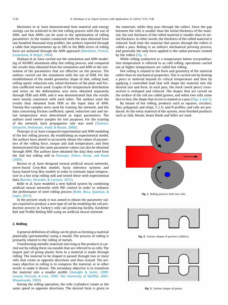
Fig. 1. Rolling process with two rolls.

7136 H. Altınkaya et al. / Expert Systems with Applications 41 (2014) 7135–7146

Martinetz et al. have demonstrated how material and energysavings can be achieved in the hot rolling process with the use ofANN, and that ANNs can be used in the optimization of rollingparameters. In the studies conducted with the data obtained fromone hundred thousand strip profiles, the authors reported througha table that improvements up to 28% in the RMS errors of rollingforce are achieved through the ANN approach (Martinetz, Protzel,Gramckow, & Sörgel, 1994).

Shahani et al. have carried out the simulation and ANN model-ing of AA5083 aluminum alloy hot rolling process, and comparedthe results they obtained from the simulation and ANN in the esti-mation of the parameters that are effective on the process. Theauthors carried out the simulation with the use of FEM. For theestablishment of the model geometric shape of slab, rolling load,rolling speed, reduction rate, initial thickness of the plate and fric-tion coefficient were used. Graphs of the temperature distributionand stress on the deformation area were obtained separatelythrough FEM and ANN, and it was demonstrated that the resultswere mostly consistent with each other. The authors used theresults they obtained from FEM as the input data of ANN.Twenty-five samples were used for training the network, and thedata concerning friction coefficient, speed, reduction rate and ini-tial temperature were determined as input parameters. Theauthors used twelve samples for test purposes. For the trainingof the network, back propagation rule was used (Shahani,Setayeshi, Nodamaie, Asadi, & Rezaie, 2009).

Öznergiz et al. have compared experimental and ANN modelingof the hot rolling process. By establishing an experimental model,the authors have aimed to accurately obtain the values of parame-ters of the rolling force, torque and slab temperature, and thendemonstrated that the same parameter values can also be obtainedthrough ANN. The authors have obtained the data they used fromthe 2nd hot rolling mill in Öznergiz, Delice, Özsoy, and Kural(2009).

Barrios et al. have designed several artificial neural networks,nerve-based Grey-Box models, fuzzy inference systems andfuzzy-based Grey-Box models in order to estimate input tempera-ture in a hot strip rolling mill and tested these with experimentaldata (Barrios, Alvarado, & Cavazos, 2012).

Rolle et al. have modeled a new hybrid system by combiningartificial neural networks with PID control in order to enhancethe performance of steel rolling process (Rolle, Roca, Quintian, &Lopez, 2013).

In the present study it was aimed to obtain the parameter val-ues required to produce a new type of rail by modeling the rail pro-duction process in Turkey’s only rail producing facility, KardemirRail and Profile Rolling Mill using an artificial neural network.

Fig. 2. Various shapes of grooves (calibres).

Fig. 3. Various shapes of passes.

2. Rolling

A general definition of rolling can be given as forming a materialplastically (permanently) using a mould. The process of rolling isprimarily related to the rolling of metals.

Transforming metallic materials into long or flat products is car-ried out by rolling them via moulds that are referred to as rolls. Thelargest part of giving plastic form to a material is made throughrolling. The material to be shaped is passed through two or morerolls that rotate at opposite directions and thus resized. The pri-mary objective in rolling is to compress the material, or in otherwords to make it denser. The secondary objective is to transformthe material into a smaller profile (Hanoglu & Sarler, 2009;Lenard, Pietrzyk, & Cser, 1999; The University of Sheffild, 2003;Wusatowski, 1969).

During the rolling operation, the rolls (cylinders) rotate at thesame speed in opposite directions. The desired form is given to

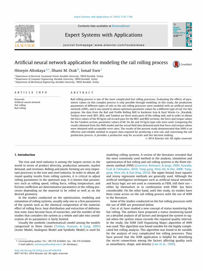
the materials, while they pass through the rollers. Since the gapbetween the rolls is smaller than the initial thickness of the mate-rial, the exit thickness of the rolled material is smaller than its ini-tial thickness. In other words, the thickness of the rolled material isreduced. Each time the material that passes through the rollers iscalled a pass. Rolling is an indirect mechanical pressing process,and generally the only force applied is the radial pressure createdby the rollers (Fig. 1).

While rolling conducted at a temperature below recrystalliza-tion temperature is referred to as cold rolling, operations carriedout at higher temperatures are called hot rolling.

Hot rolling is related to the form and geometry of the materialrather than its mechanical properties. This is carried out by heatinga piece or material beyond its critical temperature and then byapplying a controlled load that will shape the material into thedesired size and form. In each pass, the stock (work piece) cross-section is reshaped and reduced. The shapes that are carved onthe surface of the roll are called groove, and when two rolls comeface to face, the shape that occurs is named as a pass (Figs. 2 and 3).

By means of hot rolling, products such as squares, circulars,flats, polygonal, and strips, T, I, U, and H profiles, and rails are pro-duced. As the entry material of the system, semi-finished productssuch as slab, bloom, beam blank and billet are used.

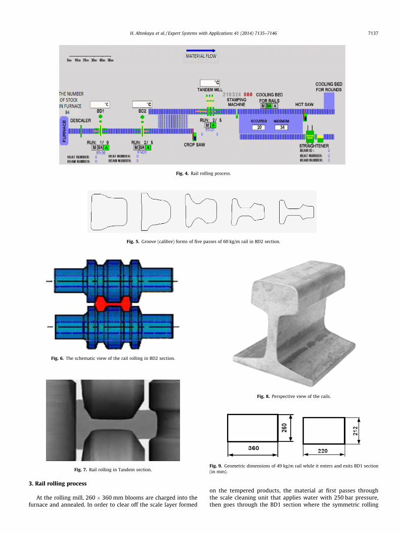
Fig. 4. Rail rolling process.

Fig. 5. Groove (calibre) forms of five passes of 60 kg/m rail in BD2 section.

Fig. 6. The schematic view of the rail rolling in BD2 section.

Fig. 7. Rail rolling in Tandem section.

Fig. 8. Perspective view of the rails.

Fig. 9. Geometric dimensions of 49 kg/m rail while it enters and exits BD1 section(in mm).

H. Altınkaya et al. / Expert Systems with Applications 41 (2014) 7135–7146 7137

3. Rail rolling process

At the rolling mill, 260 � 360 mm blooms are charged into thefurnace and annealed. In order to clear off the scale layer formed

on the tempered products, the material at first passes throughthe scale cleaning unit that applies water with 250 bar pressure,then goes through the BD1 section where the symmetric rolling

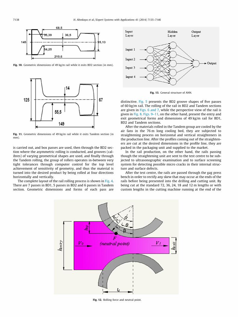
Fig. 10. Geometric dimensions of 49 kg/m rail while it exits BD2 section (in mm).

Fig. 11. Geometric dimensions of 49 kg/m rail while it exits Tandem section (inmm).

Fig. 13. General structure of ANN.

7138 H. Altınkaya et al. / Expert Systems with Applications 41 (2014) 7135–7146

is carried out, and box passes are used, then through the BD2 sec-tion where the asymmetric rolling is conducted, and grooves (cal-ibres) of varying geometrical shapes are used, and finally throughthe Tandem rolling, the group of rollers operates in-between verytight tolerances through computer control for the top levelachievement of sensitivity of geometry, and thus the material isturned into the desired product by being rolled at four directionshorizontally and vertically.

The complete layout of the rail rolling process is shown in Fig. 4.There are 7 passes in BD1, 5 passes in BD2 and 6 passes in Tandemsection. Geometric dimensions and forms of each pass are

Fig. 12. Rolling force a

distinctive. Fig. 5 presents the BD2 groove shapes of five passesof 60 kg/m rail. The rolling of the rail in BD2 and Tandem sectionsare given in Figs. 6 and 7, while the perspective view of the rail isgiven in Fig. 8. Figs. 9–11, on the other hand, present the entry andexit geometrical forms and dimensions of 49 kg/m rail for BD1,BD2 and Tandem sections.

After the materials rolled in the Tandem group are cooled by theair fans in the 76 m long cooling bed, they are subjected tostraightening process on horizontal and vertical straighteners inthe production line. After the profiles coming out of the straighten-ers are cut at the desired dimensions in the profile line, they arepacked in the packaging unit and supplied to the market.

In the rail production, on the other hand, the rails passingthough the straightening unit are sent to the test centre to be sub-jected to ultrasonographic examination and to surface screeningsystem for detecting possible micro cracks in their internal struc-ture and surface defects.

After the test centre, the rails are passed through the gag pressbench in order to rectify any skew that may occur at the ends of therails before being presented into the drilling and cutting unit. Bybeing cut at the standard 72, 36, 24, 18 and 12 m lengths or withcustom lengths in the cutting machine running at the end of the

nd neutral point.

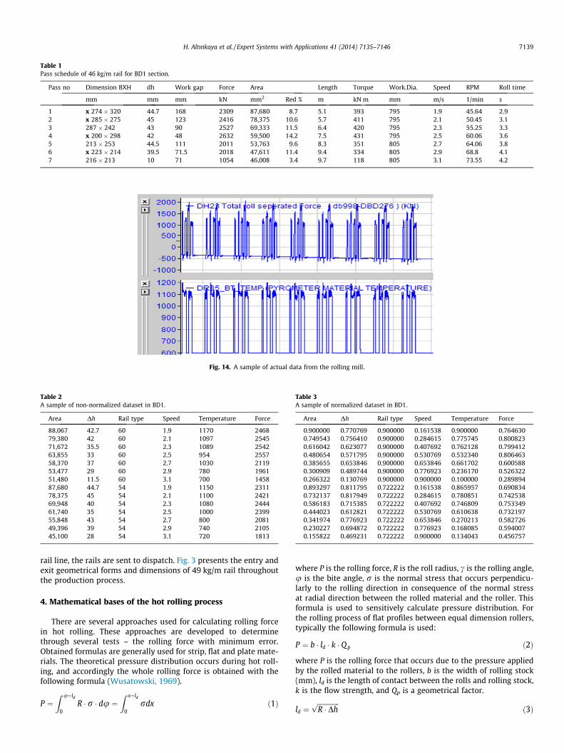
Table 1Pass schedule of 46 kg/m rail for BD1 section.

Pass no Dimension BXH dh Work gap Force Area Length Torque Work.Dia. Speed RPM Roll time

mm mm mm kN mm2 Red % m kN m mm m/s 1/min s

1 x 274 � 320 44.7 168 2309 87,680 8.7 5.1 393 795 1.9 45.64 2.92 x 285 � 275 45 123 2416 78,375 10.6 5.7 411 795 2.1 50.45 3.13 287 � 242 43 90 2527 69,333 11.5 6.4 420 795 2.3 55.25 3.34 x 200 � 298 42 48 2632 59,500 14.2 7.5 431 795 2.5 60.06 3.65 213 � 253 44.5 111 2011 53,763 9.6 8.3 351 805 2.7 64.06 3.86 x 223 � 214 39.5 71.5 2018 47,611 11.4 9.4 334 805 2.9 68.8 4.17 216 � 213 10 71 1054 46,008 3.4 9.7 118 805 3.1 73.55 4.2

Fig. 14. A sample of actual data from the rolling mill.

Table 2A sample of non-normalized dataset in BD1.

Area Dh Rail type Speed Temperature Force

88,067 42.7 60 1.9 1170 246879,380 42 60 2.1 1097 254571,672 35.5 60 2.3 1089 254263,855 33 60 2.5 954 255758,370 37 60 2.7 1030 211953,477 29 60 2.9 780 196151,480 11.5 60 3.1 700 145887,680 44.7 54 1.9 1150 231178,375 45 54 2.1 1100 242169,948 40 54 2.3 1080 244461,740 35 54 2.5 1000 239955,848 43 54 2.7 800 208149,396 39 54 2.9 740 210545,100 28 54 3.1 720 1813

Table 3A sample of normalized dataset in BD1.

Area Dh Rail type Speed Temperature Force

0.900000 0.770769 0.900000 0.161538 0.900000 0.7646300.749543 0.756410 0.900000 0.284615 0.775745 0.8008230.616042 0.623077 0.900000 0.407692 0.762128 0.7994120.480654 0.571795 0.900000 0.530769 0.532340 0.8064630.385655 0.653846 0.900000 0.653846 0.661702 0.6005880.300909 0.489744 0.900000 0.776923 0.236170 0.5263220.266322 0.130769 0.900000 0.900000 0.100000 0.2898940.893297 0.811795 0.722222 0.161538 0.865957 0.6908340.732137 0.817949 0.722222 0.284615 0.780851 0.7425380.586183 0.715385 0.722222 0.407692 0.746809 0.7533490.444023 0.612821 0.722222 0.530769 0.610638 0.7321970.341974 0.776923 0.722222 0.653846 0.270213 0.5827260.230227 0.694872 0.722222 0.776923 0.168085 0.5940070.155822 0.469231 0.722222 0.900000 0.134043 0.456757

H. Altınkaya et al. / Expert Systems with Applications 41 (2014) 7135–7146 7139

rail line, the rails are sent to dispatch. Fig. 3 presents the entry andexit geometrical forms and dimensions of 49 kg/m rail throughoutthe production process.

4. Mathematical bases of the hot rolling process

There are several approaches used for calculating rolling forcein hot rolling. These approaches are developed to determinethrough several tests – the rolling force with minimum error.Obtained formulas are generally used for strip, flat and plate mate-rials. The theoretical pressure distribution occurs during hot roll-ing, and accordingly the whole rolling force is obtained with thefollowing formula (Wusatowski, 1969).

P ¼Z u¼ld

0R � r � du ¼

Z x¼ld

0rdx ð1Þ

where P is the rolling force, R is the roll radius, c is the rolling angle,u is the bite angle, r is the normal stress that occurs perpendicu-larly to the rolling direction in consequence of the normal stressat radial direction between the rolled material and the roller. Thisformula is used to sensitively calculate pressure distribution. Forthe rolling process of flat profiles between equal dimension rollers,typically the following formula is used:

P ¼ b � ld � k � Q p ð2Þ

where P is the rolling force that occurs due to the pressure appliedby the rolled material to the rollers, b is the width of rolling stock(mm), ld is the length of contact between the rolls and rolling stock,k is the flow strength, and Qp is a geometrical factor.

ld ¼ffiffiffiffiffiffiffiffiffiffiffiffiffiR � Dhp

ð3Þ

7140 H. Altınkaya et al. / Expert Systems with Applications 41 (2014) 7135–7146

ld is signified as shown above. Here, while R is the radius of the rolls,Dh is the reduction rate. Celikow, Glowin, Samarin, Orowan, Pascoe,Sims and Ekelund proposed different equations for calculating thegeometrical factor Qp, based on their own experimental rolling data.Here only Sims’ and Ekelund’s equations will be provided withoutgoing into details. According to Sims (Hanoglu & Sarler, 2009;Wusatowski, 1969):

Q p ¼p2

ffiffiffiffiffiffiffiffiffiffiffi1� r

r

rtan�1

ffiffiffiffiffiffiffiffiffiffiffir

1� r

r� p

4�

ffiffiffiffiffiffiffiffiffiffiffi1� r

r

rR0

hexitln

hnp

hexit

"

þ 12

ffiffiffiffiffiffiffiffiffiffiffi1� r

r

rR0

hexitln

11� r

#ð4Þ

where hnp is the thickness at the neutral point as seen in Fig. 12, r(Dh) is the reduction (hentry � hexit). And the symbol R0 is given by

R0 ¼ R 1þ16 1� v2� �pEDh

Pr

� �ð5Þ

where R0 is the flattened but still circular roll radius, R is the originalroll radius, v is the Poisson’s ratio, E is the Young’s modulus of theroll in Pa, and Pr is the roll separating force, as shown in Fig. 12.

According to Ekelund (Wusatowski, 1969):

Q p ¼ 1þ 1:6:l:ffiffiffiffiffiffiffiffiffiffiffiffiffiffiffiffiffiffiffiffiffiffiRðh0 � h1Þ

p� 1:2:ðh0 � h1Þ

h0 þ h1ð6Þ

For rail and profile rolling processes, these formulas will bemuch more complex. In the limited number of studies conductedon rail rolling, which is a non-linear and complex process,researchers proposed some formulas for force on the basis of theirown experimental data. Here, only the formula for the force on thehorizontal roller in the Tandem section will be provided (Yang-gang et al., 2010).

Ph ¼Rh

2whLwVhNw þ Nhb þ Nht þ N3 þ N03 þ N4 þ N5� �

ð7Þ

where, Ph is the rolling force acting on the horizontal roll, Rh is theradius of horizontal roll, Vh is the length of deformation zone

Fig. 15. Architectu

Fig. 16. View of the

between horizontal roll and web of rail, wh is the neutral angle ofthe horizontal roll, Nx is the power consumed on the discontinuityvarious surface of plastic deformation region.

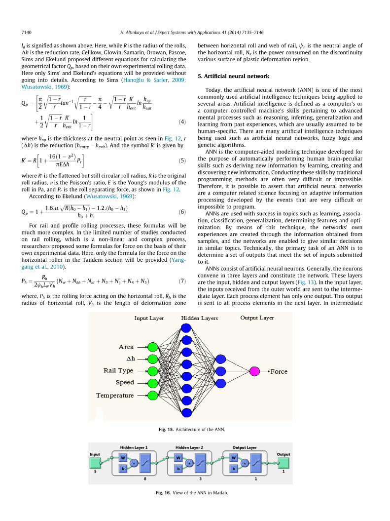
5. Artificial neural network

Today, the artificial neural network (ANN) is one of the mostcommonly used artificial intelligence techniques being applied toseveral areas. Artificial intelligence is defined as a computer’s ora computer controlled machine’s skills pertaining to advancedmental processes such as reasoning, inferring, generalization andlearning from past experiences, which are usually assumed to behuman-specific. There are many artificial intelligence techniquesbeing used such as artificial neural networks, fuzzy logic andgenetic algorithms.

ANN is the computer-aided modeling technique developed forthe purpose of automatically performing human brain-peculiarskills such as deriving new information by learning, creating anddiscovering new information. Conducting these skills by traditionalprogramming methods are often very difficult or impossible.Therefore, it is possible to assert that artificial neural networksare a computer related science focusing on adaptive informationprocessing developed by the events that are very difficult orimpossible to program.

ANNs are used with success in topics such as learning, associa-tion, classification, generalization, determining features and opti-mization. By means of this technique, the networks’ ownexperiences are created through the information obtained fromsamples, and the networks are enabled to give similar decisionsin similar topics. Technically, the primary task of an ANN is todetermine a set of outputs that meet the set of inputs submittedto it.

ANNs consist of artificial neural neurons. Generally, the neuronsconvene in three layers and constitute the network. These layersare the input, hidden and output layers (Fig. 13). In the input layer,the inputs received from the outer world are sent to the interme-diate layer. Each process element has only one output. This outputis sent to all process elements in the next layer. In intermediate

re of the ANN.

ANN in Matlab.

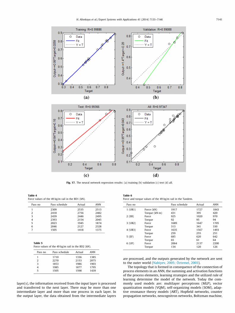
Fig. 17. The neural network regression results: (a) training (b) validation (c) test (d) all.

Table 4Force values of the 49 kg/m rail in the BD1 (kN).

Pass no Pass schedule Actual ANN

1 2309 2535 25132 2418 2756 24823 2439 2446 24954 2393 2154 20455 2023 1945 18746 2046 2127 23287 1505 1418 1375

Table 5Force values of the 49 kg/m rail in the BD2 (kN).

Pass no Pass schedule Actual ANN

1 1710 1336 13852 2270 2153 20753 1853 1986 19034 1985 1877 17955 1505 1598 1439

Table 6Force and torque values of the 49 kg/m rail in the Tandem.

Pass no Pass schedule Actual ANN

1 (UR1) Force (kN) 1917 1727 1843Torque (kN m) 431 395 420

2 (ER) Force 925 1020 970Torque 92 95 94

3 (UR2) Force 1689 1647 1705Torque 313 341 330

4 (UR3) Force 1635 1567 1493Torque 259 255 251

5 (EF) Force 685 620 642Torque 65 61 64

6 (UF) Force 2064 2137 2200Torque 134 120 126

H. Altınkaya et al. / Expert Systems with Applications 41 (2014) 7135–7146 7141

layer(s), the information received from the input layer is processedand transferred to the next layer. There may be more than oneintermediate layer and more than one process in each layer. Inthe output layer, the data obtained from the intermediate layers

are processed, and the outputs generated by the network are sentto the outer world (Nabiyev, 2005; Öztemel, 2003).

The topology that is formed in consequence of the connection ofprocess elements in an ANN, the summing and activation functionsof the process elements, learning strategies and the utilized rule oflearning determine the model of the network. Today the com-monly used models are: multilayer perceptrons (MLP), vectorquantization models (VQM), self-organizing models (SOM), adap-tive resonance theory models (ART), Hopfield networks, counterpropagation networks, neocognitron networks, Boltzman machine,

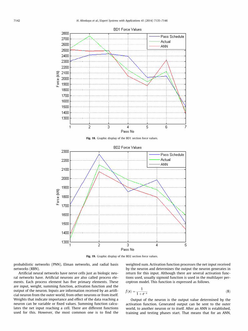
Fig. 18. Graphic display of the BD1 section force values.

Fig. 19. Graphic display of the BD2 section force values.

7142 H. Altınkaya et al. / Expert Systems with Applications 41 (2014) 7135–7146

probabilistic networks (PNN), Elman networks, and radial basisnetworks (RBN).

Artificial neural networks have nerve cells just as biologic neu-ral networks have. Artificial neurons are also called process ele-ments. Each process element has five primary elements. Theseare input, weight, summing function, activation function and theoutput of the neuron. Inputs are information received by an artifi-cial neuron from the outer world, from other neurons or from itself.Weights that indicate importance and effect of the data reaching aneuron can be variable or fixed values. Summing function calcu-lates the net input reaching a cell. There are different functionsused for this. However, the most common one is to find the

weighted sum. Activation function processes the net input receivedby the neuron and determines the output the neuron generates inreturn for this input. Although there are several activation func-tions used, usually sigmoid function is used in the multilayer per-ceptron model. This function is expressed as follows.

f ðxÞ ¼ 11þ e�x

ð8Þ

Output of the neuron is the output value determined by theactivation function. Generated output can be sent to the outerworld, to another neuron or to itself. After an ANN is established,training and testing phases start. That means that for an ANN,

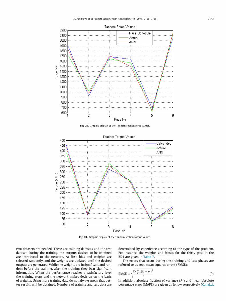
Fig. 20. Graphic display of the Tandem section force values.

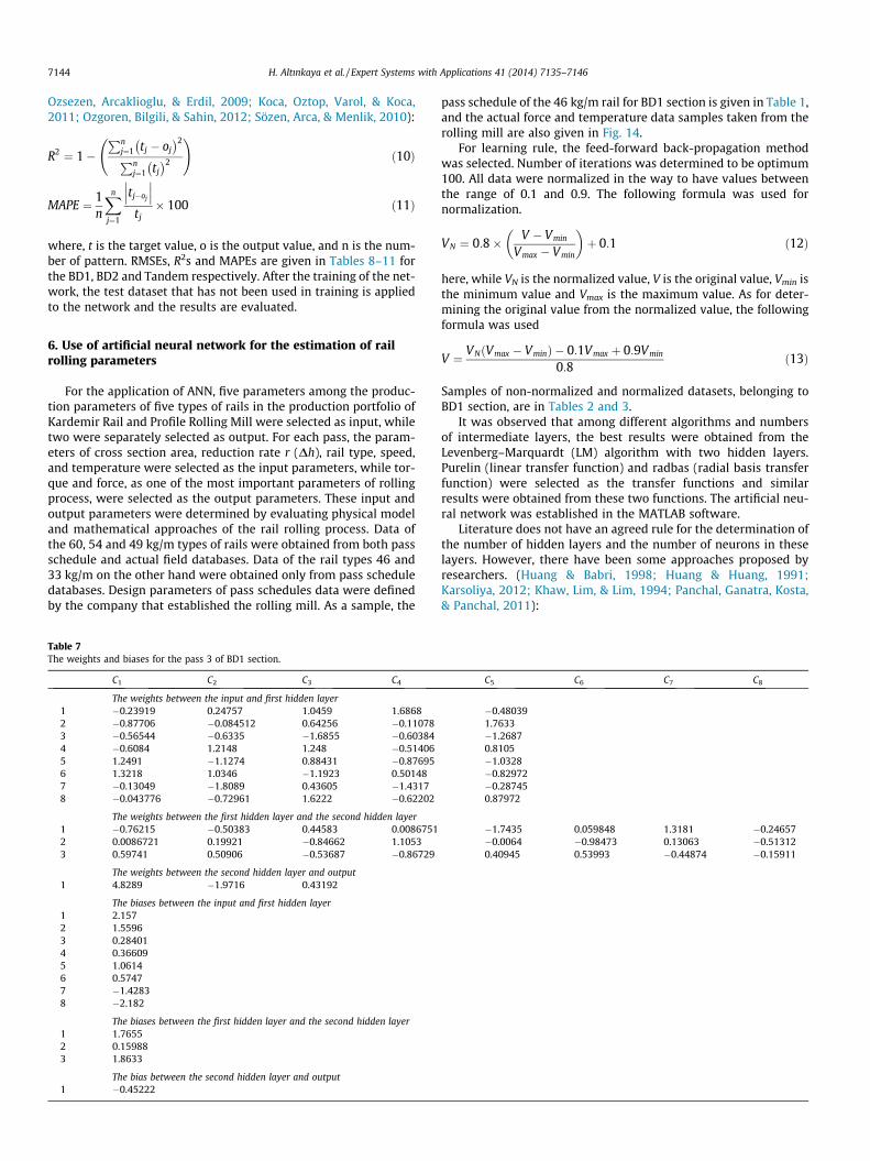
Fig. 21. Graphic display of the Tandem section torque values.

H. Altınkaya et al. / Expert Systems with Applications 41 (2014) 7135–7146 7143

two datasets are needed. These are training datasets and the testdataset. During the training, the outputs desired to be obtainedare introduced to the network. At first, bias and weights areselected randomly, and the weights are updated until the desiredoutputs are generated. While the weights are insignificant and ran-dom before the training, after the training they bear significantinformation. When the performance reaches a satisfactory levelthe training stops and the network makes decision on the basisof weights. Using more training data do not always mean that bet-ter results will be obtained. Numbers of training and test data are

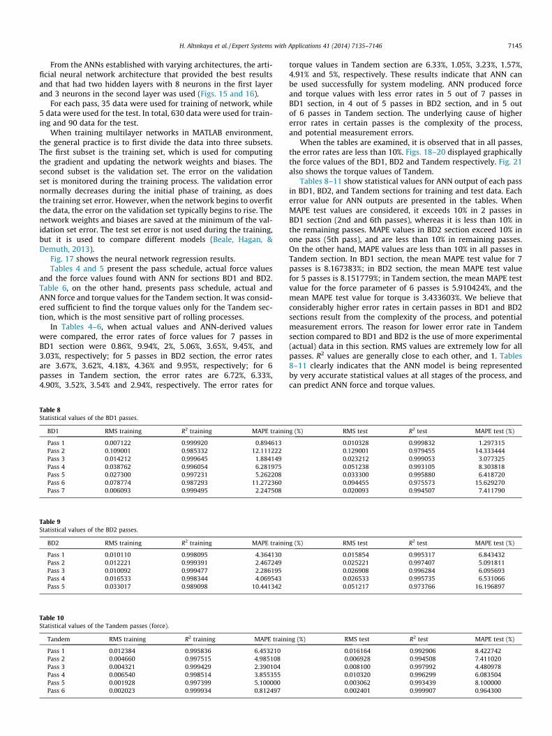
determined by experience according to the type of the problem.For instance, the weights and biases for the thirty pass in theBD1 are given in Table 7.

The errors that occur during the training and test phases arereferred to as root mean squares errors (RMSE):

RMSE ¼

ffiffiffiffiffiffiffiffiffiffiffiffiffiffiffiffiffiffiffiffiffiffiffiffiffiffiffiffiffiPnj¼1ðtj � ojÞ2

n

sð9Þ

In addition, absolute fraction of variance (R2) and mean absolutepercentage error (MAPE) are given as follow respectively (Canakci,

7144 H. Altınkaya et al. / Expert Systems with Applications 41 (2014) 7135–7146

Ozsezen, Arcaklioglu, & Erdil, 2009; Koca, Oztop, Varol, & Koca,2011; Ozgoren, Bilgili, & Sahin, 2012; Sözen, Arca, & Menlik, 2010):

R2 ¼ 1�Pn

j¼1 tj � oj� �2

Pnj¼1 tj� �2

!ð10Þ

MAPE ¼ 1n

Xn

j¼1

tj�oj

��� ���tj� 100 ð11Þ

where, t is the target value, o is the output value, and n is the num-ber of pattern. RMSEs, R2s and MAPEs are given in Tables 8–11 forthe BD1, BD2 and Tandem respectively. After the training of the net-work, the test dataset that has not been used in training is appliedto the network and the results are evaluated.

6. Use of artificial neural network for the estimation of railrolling parameters

For the application of ANN, five parameters among the produc-tion parameters of five types of rails in the production portfolio ofKardemir Rail and Profile Rolling Mill were selected as input, whiletwo were separately selected as output. For each pass, the param-eters of cross section area, reduction rate r (Dh), rail type, speed,and temperature were selected as the input parameters, while tor-que and force, as one of the most important parameters of rollingprocess, were selected as the output parameters. These input andoutput parameters were determined by evaluating physical modeland mathematical approaches of the rail rolling process. Data ofthe 60, 54 and 49 kg/m types of rails were obtained from both passschedule and actual field databases. Data of the rail types 46 and33 kg/m on the other hand were obtained only from pass scheduledatabases. Design parameters of pass schedules data were definedby the company that established the rolling mill. As a sample, the

Table 7The weights and biases for the pass 3 of BD1 section.

C1 C2 C3 C4

The weights between the input and first hidden layer1 �0.23919 0.24757 1.0459 1.68682 �0.87706 �0.084512 0.64256 �0.110783 �0.56544 �0.6335 �1.6855 �0.603844 �0.6084 1.2148 1.248 �0.514065 1.2491 �1.1274 0.88431 �0.876956 1.3218 1.0346 �1.1923 0.501487 �0.13049 �1.8089 0.43605 �1.43178 �0.043776 �0.72961 1.6222 �0.62202

The weights between the first hidden layer and the second hidden layer1 �0.76215 �0.50383 0.44583 0.00867512 0.0086721 0.19921 �0.84662 1.10533 0.59741 0.50906 �0.53687 �0.86729

The weights between the second hidden layer and output1 4.8289 �1.9716 0.43192

The biases between the input and first hidden layer1 2.1572 1.55963 0.284014 0.366095 1.06146 0.57477 �1.42838 �2.182

The biases between the first hidden layer and the second hidden layer1 1.76552 0.159883 1.8633

The bias between the second hidden layer and output1 �0.45222

pass schedule of the 46 kg/m rail for BD1 section is given in Table 1,and the actual force and temperature data samples taken from therolling mill are also given in Fig. 14.

For learning rule, the feed-forward back-propagation methodwas selected. Number of iterations was determined to be optimum100. All data were normalized in the way to have values betweenthe range of 0.1 and 0.9. The following formula was used fornormalization.

VN ¼ 0:8� V � Vmin

Vmax � Vmin

� þ 0:1 ð12Þ

here, while VN is the normalized value, V is the original value, Vmin isthe minimum value and Vmax is the maximum value. As for deter-mining the original value from the normalized value, the followingformula was used

V ¼ VN Vmax � Vminð Þ � 0:1Vmax þ 0:9Vmin

0:8ð13Þ

Samples of non-normalized and normalized datasets, belonging toBD1 section, are in Tables 2 and 3.

It was observed that among different algorithms and numbersof intermediate layers, the best results were obtained from theLevenberg–Marquardt (LM) algorithm with two hidden layers.Purelin (linear transfer function) and radbas (radial basis transferfunction) were selected as the transfer functions and similarresults were obtained from these two functions. The artificial neu-ral network was established in the MATLAB software.

Literature does not have an agreed rule for the determination ofthe number of hidden layers and the number of neurons in theselayers. However, there have been some approaches proposed byresearchers. (Huang & Babri, 1998; Huang & Huang, 1991;Karsoliya, 2012; Khaw, Lim, & Lim, 1994; Panchal, Ganatra, Kosta,& Panchal, 2011):

C5 C6 C7 C8

�0.480391.7633�1.26870.8105�1.0328�0.82972�0.287450.87972

�1.7435 0.059848 1.3181 �0.24657�0.0064 �0.98473 0.13063 �0.513120.40945 0.53993 �0.44874 �0.15911

H. Altınkaya et al. / Expert Systems with Applications 41 (2014) 7135–7146 7145

From the ANNs established with varying architectures, the arti-ficial neural network architecture that provided the best resultsand that had two hidden layers with 8 neurons in the first layerand 3 neurons in the second layer was used (Figs. 15 and 16).

For each pass, 35 data were used for training of network, while5 data were used for the test. In total, 630 data were used for train-ing and 90 data for the test.

When training multilayer networks in MATLAB environment,the general practice is to first divide the data into three subsets.The first subset is the training set, which is used for computingthe gradient and updating the network weights and biases. Thesecond subset is the validation set. The error on the validationset is monitored during the training process. The validation errornormally decreases during the initial phase of training, as doesthe training set error. However, when the network begins to overfitthe data, the error on the validation set typically begins to rise. Thenetwork weights and biases are saved at the minimum of the val-idation set error. The test set error is not used during the training,but it is used to compare different models (Beale, Hagan, &Demuth, 2013).

Fig. 17 shows the neural network regression results.Tables 4 and 5 present the pass schedule, actual force values

and the force values found with ANN for sections BD1 and BD2.Table 6, on the other hand, presents pass schedule, actual andANN force and torque values for the Tandem section. It was consid-ered sufficient to find the torque values only for the Tandem sec-tion, which is the most sensitive part of rolling processes.

In Tables 4–6, when actual values and ANN-derived valueswere compared, the error rates of force values for 7 passes inBD1 section were 0.86%, 9.94%, 2%, 5.06%, 3.65%, 9.45%, and3.03%, respectively; for 5 passes in BD2 section, the error ratesare 3.67%, 3.62%, 4.18%, 4.36% and 9.95%, respectively; for 6passes in Tandem section, the error rates are 6.72%, 6.33%,4.90%, 3.52%, 3.54% and 2.94%, respectively. The error rates for

Table 8Statistical values of the BD1 passes.

BD1 RMS training R2 training MAPE trainin

Pass 1 0.007122 0.999920 0.894613Pass 2 0.109001 0.985332 12.111222Pass 3 0.014212 0.999645 1.884149Pass 4 0.038762 0.996054 6.281975Pass 5 0.027300 0.997231 5.262208Pass 6 0.078774 0.987293 11.272360Pass 7 0.006093 0.999495 2.247508

Table 9Statistical values of the BD2 passes.

BD2 RMS training R2 training MAPE trainin

Pass 1 0.010110 0.998095 4.364130Pass 2 0.012221 0.999391 2.467249Pass 3 0.010092 0.999477 2.286195Pass 4 0.016533 0.998344 4.069543Pass 5 0.033017 0.989098 10.441342

Table 10Statistical values of the Tandem passes (force).

Tandem RMS training R2 training MAPE traini

Pass 1 0.012384 0.995836 6.453210Pass 2 0.004660 0.997515 4.985108Pass 3 0.004321 0.999429 2.390104Pass 4 0.006540 0.998514 3.855355Pass 5 0.001928 0.997399 5.100000Pass 6 0.002023 0.999934 0.812497

torque values in Tandem section are 6.33%, 1.05%, 3.23%, 1.57%,4.91% and 5%, respectively. These results indicate that ANN canbe used successfully for system modeling. ANN produced forceand torque values with less error rates in 5 out of 7 passes inBD1 section, in 4 out of 5 passes in BD2 section, and in 5 outof 6 passes in Tandem section. The underlying cause of highererror rates in certain passes is the complexity of the process,and potential measurement errors.

When the tables are examined, it is observed that in all passes,the error rates are less than 10%. Figs. 18–20 displayed graphicallythe force values of the BD1, BD2 and Tandem respectively. Fig. 21also shows the torque values of Tandem.

Tables 8–11 show statistical values for ANN output of each passin BD1, BD2, and Tandem sections for training and test data. Eacherror value for ANN outputs are presented in the tables. WhenMAPE test values are considered, it exceeds 10% in 2 passes inBD1 section (2nd and 6th passes), whereas it is less than 10% inthe remaining passes. MAPE values in BD2 section exceed 10% inone pass (5th pass), and are less than 10% in remaining passes.On the other hand, MAPE values are less than 10% in all passes inTandem section. In BD1 section, the mean MAPE test value for 7passes is 8.167383%; in BD2 section, the mean MAPE test valuefor 5 passes is 8.151779%; in Tandem section, the mean MAPE testvalue for the force parameter of 6 passes is 5.910424%, and themean MAPE test value for torque is 3.433603%. We believe thatconsiderably higher error rates in certain passes in BD1 and BD2sections result from the complexity of the process, and potentialmeasurement errors. The reason for lower error rate in Tandemsection compared to BD1 and BD2 is the use of more experimental(actual) data in this section. RMS values are extremely low for allpasses. R2 values are generally close to each other, and 1. Tables8–11 clearly indicates that the ANN model is being representedby very accurate statistical values at all stages of the process, andcan predict ANN force and torque values.

g (%) RMS test R2 test MAPE test (%)

0.010328 0.999832 1.2973150.129001 0.979455 14.3334440.023212 0.999053 3.0773250.051238 0.993105 8.3038180.033300 0.995880 6.4187200.094455 0.975573 15.6292700.020093 0.994507 7.411790

g (%) RMS test R2 test MAPE test (%)

0.015854 0.995317 6.8434320.025221 0.997407 5.0918110.026908 0.996284 6.0956930.026533 0.995735 6.5310660.051217 0.973766 16.196897

ng (%) RMS test R2 test MAPE test (%)

0.016164 0.992906 8.4227420.006928 0.994508 7.4110200.008100 0.997992 4.4809780.010320 0.996299 6.0835040.003062 0.993439 8.1000000.002401 0.999907 0.964300

Table 11Statistical values of the Tandem passes (torque).

Tandem RMS training R2 training MAPE training (%) RMS test R2 test MAPE test (%)

Pass 1 0.006750 0.999057 3.071429 0.013553 0.996197 6.167183Pass 2 0.000344 0.999963 0.610036 0.000533 0.999911 0.945586Pass 3 0.005482 0.999171 2.879964 0.005860 0.999052 3.078533Pass 4 0.001754 0.999851 1.222117 0.002132 0.999779 1.485524Pass 5 0.001332 0.998759 3.523000 0.001625 0.998151 4.300000Pass 6 0.002857 0.998332 4.084387 0.003235 0.997861 4.624796

7146 H. Altınkaya et al. / Expert Systems with Applications 41 (2014) 7135–7146

7. Conclusions

The current study revealed that by using the production param-eters of four different types of rails (60, 54, 46 and 33 kg/m), theparameter values of a new type of rail (49 kg/m) can be obtainedby modeling with ANN. Comparing the results obtained fromANN and the production values to determine the torque and forcevalues of 49 kg/m rail showed that the error rates in all passes arebelow 10%. It was demonstrated that by modeling the productionparameter values of present rails with ANN, the important param-eter values required for the production of a new (different) type ofrail can be obtained. The low rates of error indicate the reliability ofthe model. It was observed that the selections made in the deter-mination of input parameters for accurately calculating the forceand torque values accepted as output parameters are significantlyeffective on the results. It was also observed that using the normal-ized data and actual field data enable researchers to obtain betterresults.

This study showed clearly that instead of using complexapproaches and analytical equations, ANNs can be used to deter-mine parameter values required for product design in the rail roll-ing process. In addition, in an extremely complicated andexpensive system such as rail rolling, it is possible to simulate anew product by using ANN, without causing time and financialloss.

Rail rolling process is one of the most complicated rolling pro-cesses. Therefore it is difficult to introduce mathematical modelwith high accuracy for the process. In present study it is shownthat ANN algorithm can be used as an alternative method in mod-eling and simulation of the process.

For future studies, ANN algorithm can be integrated with theprocess of designing intermediate passes by evaluating force andtorque values. Considering the parameters which can be changedin real time operation such as Dh, area, temperature, ANNalgorithm can be implemented for online simulation of rail rollingprocess. It is also possible to investigate applicability of using thismodel in the real time control systems.

Acknowledgments

The authors wish to thank Kardemir Iron & Steel Works Co. stafffor their contribution to this project by providing data related torail rolling and for helpful encouragement during the validationof the result of the research in this study.

References

Barrios, J. A., Alvarado, M. T., & Cavazos, A. (2012). Neural, fuzzy and grey-boxmodelling for entry temperature prediction in a hot strip mill. Expert Systemswith Applications, 39, 3374–3384.

Beale, M. H., Hagan, M. T., & Demuth, H. B. (2013). Neural network toolbox user’sguide. MathWorks, Technical Support.

Canakci, M., Ozsezen, A. N., Arcaklioglu, E., & Erdil, A. (2009). Prediction ofperformance and exhaust emissions of a diesel engine fuelled with biodieselproduced from waste frying palm oil. Expert Systems with Applications, 36,9268–9280.

Cser, L., Korhonen, A. S., Gulyas, J. Mantyla, P., Simula, O., & Reiss, Gy., et al. (1999).Data mining and state monitoring in hot rolling. Bay Zoltan Institute forLogistics and Production Systems, H3519, Miskolc-Tapolca, Hungry.

Guerrero, M. A., Belzunce, J., & Jorge, J. (2009). Hot rolling process simulation.Application to UIC-60 rail rolling. In Proceedings of the 4th IASME/WSEASinternational conference on continuum mechanics (CM’09).

Hanoglu, U. & Sarler, B. (2009). Mathematical and physical modelling of the flatrolling process. www.sabotin.ung.si/~sstanic/teaching/.../20090924_Hanoglu_Rolling.pdf.

Huang, G. B., & Babri, H. A. (1998). Upper bounds on the number of hidden neuronsin feed forward networks with arbitrary bounded nonlinear activationfunctions. IEEE Transactions on Neural Networks, 9(1).

Huang, S. C., & Huang, Y. F. (1991). Bounds on the number of hidden neurons inmultilayer perceptrons. IEEE Transactions on Neural Networks, 2(1), 47–55.

Karsoliya, S. (2012). Approximating number of hidden layer neurons in multiplehidden layer BPNN architecture. International Journal of Engineering Trends andTechnology, 3(6), 714–717. ISSN: 2231-5381.

Kawalla, R., Graf, M., & Tokmakov, K. (2010). Simulation system of multistage hotrolling process of flat products. METABK, 49(3), 175–179. ISSN: 0543-5846.

Khaw, J. F. C., Lim, B. S., & Lim, L. E. N. (1994). Optimal design of neural networksusing the Taguchi method. Neurocomputing, 7(225–245).

Koca, A., Oztop, H. F., Varol, Y., & Koca, G. O. (2011). Estimation of solar radiationusing artificial neural networks with different input parameters forMediterranean region of Anatolia in Turkey. Expert Systems with Applications,38, 8756–8762.

Lenard, J. G., Pietrzyk, M., & Cser, L. (1999). Mathematical and physical simulation ofthe properties of hot rolled products. U.K: Elsevier.

Martinetz, T., Protzel, P., Gramckow, O., & Sörgel, G. (1994). Neural network controlfor rolling mills. München, Germany: Siemens AG Corporate R&D.

Nabiyev, V. V. (2005). Artificial intelligence. Seckin publishing.Ozgoren, M., Bilgili, M., & Sahin, B. (2012). Estimation of global solar radiation using

ANN over Turkey. Expert Systems with Applications, 39, 5043–5051.Öznergiz, E., Delice, I., Özsoy, C., & Kural, A. (2009). Comparison of empirical and

neural network hot-rolling process models. Proceedings of The Institution ofMechanical Engineers, Part B, Journal of Engineering Manufacture, 26, 305–312.http://dx.doi.org/10.1243/09544054JEM1290.

Öztemel, E. (2003). Artificial neural networks. Seckin publishing.Panchal, G., Ganatra, A., Kosta, Y. P., & Panchal, D. (2011). International Journal of

Computer Theory and Engineering 3(2). ISSN: 1793-8201.Rolle, J. L. C., Roca, J. L. C., Quintian, H., & Lopez, M. C. M. (2013). A hybrid intelligent

system for PID controller using in a steel rolling process. Expert Systems withApplications, 40, 5188–5196.

Shahani, A. R., Setayeshi, S., Nodamaie, S. A., Asadi, M. A., & Rezaie, S. (2009).Prediction of influence parameters on the hot rolling process using finiteelement method and neural network. Journal of Materials Processing Technology,2, 1920–1935.

Sözen, A., Arca & Menlik, T. (2010). Derivation of empirical for thermodynamicproperties of a ozone safe refrigerant using artificial neural network. ExpertSystems with Applications, 37, 1158–1168.

The University of Sheffild, case studies (2003). Technology of flat rolling.Turban, E., Aranson, J. E., & Liang, T. P. (2005). Decision support systems and intelligent

systems (seventh ed.). New Jersey: Pearson Education Inc., pp. 47–48.Wusatowski, Z. (1969). Fundamentals of rolling. Oxford, U.K: Pergomon Press.Yang-gang, D., Wen-zhi, Z., & Hui, C. (2008). Determination of forward slip

coefficient during heavy rail rolling using universal mill. Journal of Iron and SteelResearch, International, 15(2), 32–38.

Yang-gang, D., Wen-zhi, Z., & Iian-feng, S. (2010). Theoretical and experimentalresearch on rolling force for rail hot rolling by universal mill. InternationalJournal of Iron and Steel Research, 17(1), 27–32.