arX

iv:n

lin/0

5020

60v1

[nl

in.C

D]

25

Feb

2005

Mesoscopic modeling of heterogeneous boundary conditions

for microchannel flows

R. Benzi1, L. Biferale1, M. Sbragaglia1, S. Succi2 and F. Toschi2

1 Dipartimento di Fisica, Universita “Tor Vergata”, and INFN,

Via della Ricerca Scientifica 1, I-00133 Roma, Italy.2 CNR, IAC, Viale del Policlinico 137, I-00161 Roma, Italy.

December 29, 2013

Abstract

We present a mesoscopic model of the fluid-wall interactions for flows in microchannelgeometries. We define a suitable implementation of the boundary conditions for a discreteversion of the Boltzmann equations describing a wall-bounded single phase fluid. We dis-tinguish different slippage properties on the surface by introducing a slip function, definingthe local degree of slip for mesoscopic molecules at the boundaries. The slip function playsthe role of a renormalizing factor which incorporates, with some degree of arbitrariness, themicroscopic effects on the mesoscopic description. We discuss the mesoscopic slip propertiesin terms of slip length, slip velocity, pressure drop reduction (drag reduction), and mass flowrate in microchannels as a function of the degree of slippage and of its spatial distribution andlocalization, the latter parameter mimicking the degree of roughness of the ultra-hydrophobicmaterial in real experiments. We also discuss the increment of the slip length in the transi-

tion regime, i.e. at O(1) Knudsen numbers. Finally, we compare our results with MolecularDynamics investigations of the dependency of the slip length on the mean channel pressureand local slip properties (Cottin-Bizonne et al. 2004) and with the experimental dependencyof the pressure drop reduction on the percentage of hydrophobic material deposited on thesurface – Ou et al. (2004).

1 Introduction

The physics of molecular interactions at fluid-solid interfaces is a very active research area witha significant impact on many emerging applications in material science, chemistry, micro/nano-engineering, biology and medicine, see Whitesides & Stroock (2001), Lion et al. (2003), Gad-el’Hak(1999), Ho & Tai (1998). As for most problems connected with surface effects, fluid-solid inter-actions become particularly important for micro- and nano-devices, whose physical behaviour islargely affected by high surface/volume ratios. Recently, due to an ever-increasing interest in mi-crofluidics and MEMS (micro-electromechanical system)-based devices, experimental capabilitiesto test and analyze such systems have undergone remarkable progress.

In this paper, we shall focus on flows in micro-channels, a subject which has recently becomeaccessible to systematic experimental studies thanks to the developments of silicon technology (seeTabeling (2003), Karniadakis & Benskok (2002) and references therein).

Classical hydrodynamics postulates that a fluid flowing over a solid wall sticks to the bound-aries, i.e. the fluid molecules share the same velocity of the surface, Batchelor (1989); Massey(1989). This law, and its consequences, are well verified at a macroscopic level, where the char-acteristic scales of the flow are much larger than the molecular sizes. The situation changesdrastically at a microscopic level. Many experiments (Maurer et al. (2004); Ou et al. (2004);Watanabe et al. (1999); Vinogradova & Yabukov (2003); Vinogranova (1999); Pit et al. (2000);Baudry et al. (2001); Craig et al. (2001); Zhu & Granick (2001, 2002); Cheng & Giordano (2002);

1

Tretheway & Meinhart (2002); Bonnacurso et al. (2002, 2003); Choi et al. (2003); Zhang et al.(2002)) and numerical simulations using Molecular Dynamics (Barrat & Bocquet (1999a,b); Thompson & Troian(1997); Thompson & Robbins (1990); Bocquet & Barrat (1993); Cieplak et al. (2001); Thompson & Robbins(1989); Priezjev et al. (2004)) have shown evidences that the solid-fluid interactions are stronglyaffected by the chemico-physical properties and by the roughness of the surface. For example,water flowing over a hydrophilic, hydrophobic or super-hydrophobic surface, may develop quitedifferent flow profiles in micro-structures. One of the most spectacular effect is the appearanceof an effective slip velocity, Vs, at the boundary, which, in turn, may imply a reduction of thekinetic energy dissipation with significant enhancement of the overall throughput (at a givenpressure drop), see Watanabe et al. (1999); Vinogradova & Yabukov (2003); Pit et al. (2000);Baudry et al. (2001); Craig et al. (2001); Zhu & Granick (2001, 2002); Cheng & Giordano (2002);Tretheway & Meinhart (2002); Bonnacurso et al. (2002); Choi et al. (2003). From the slip veloc-ity, one defines a slip length, Ls, as the distance from the wall where the linearly extrapolatedvelocity profile vanishes. The experimental and theoretical picture is still under active develop-ment. No clear systematic trend of the slip effect as a function of the chemico-physical componentshas been found to date. Slip lengths varying from hundreds of nm up to tens of µm have beenreported in the literature. Moreover, controversial claims about the importance of the roughnessof the surface and of the combined degree of roughness-hydrophobicity have been presented. Insimple flows roughness is expected to increase the energy exchange with the boundaries, inducinga corresponding decrease in the slippage. However, both increase and decrease of the slip lengthas a function of the surface roughness have been claimed in the literature, Zhu & Granick (2001,2002); Bonnacurso et al. (2002, 2003). From a purely molecular point of view, a critical parametergoverning the solid-liquid interface is the contact angle (wetting angle). Clean glass is highly hy-drophilic, with an angle with water close to θ = 0o (perfect wetting). Recently ultra-hydrophobicsurfaces have been obtained which prove capable of sustaining a contact angle with water as highas θ = 177o a value at which water droplets are almost spherical on the surface, Chen et al. (1999);Fadeev & Carthy (1999).

Some authors proposed that the increase in the slippage might be due to a rarefaction of theflow close to the wall, a depleted water region or vapor layer should exists near a hydrophobicsurface in contact with water, Lum et al. (1999); Sakurai et al. (1998); Schwendel et al. (2003);Tyrrell & Attard (2001). Recent Molecular Dynamics simulations have also presented some evi-dences of a dewetting transition, leading to a strong increase of the slip length, below some capillar-ity pressure in microchannels with heterogeneous surface, Cottin-Bizonne et al. (2003, 2004). Thephysics looks very fragile, depending as it seems on many complicated chemical and geometricaldetails.

From the numerical point of view, Molecular Dynamics (MD) is the standard tool to system-atically investigate the problem, Frenkel & Smit (1995); Rapaport (1995); Boon & Yip (1991).In MD the solid-liquid and the liquid-liquid interactions are introduced by using Lennard-Jonestype potential (with interaction energies and molecular diameters adjusted from experiments).By changing the interaction energies one may tune the surface tension and, consequently, thecontact angles. MD also offers the possibility to model the boundary geometries and roughnesswith a high degree of fidelity. The main limitation, however, is the modest range of space andespecially time-scales, which can be simulated at a reasonable computational time, typically a fewnanoseconds, Rapaport (1995); Koplik & Banavar (1991).

The coupling between MD and hydrodynamic modes involves a huge gap of space and timescales. Recently, an interesting attempt to reproduce MD simulations of heterogeneous mi-crochannels with a continuum mechanical description based on Navier-Stokes equations and suit-able hydrodynamic boundary conditions has been proposed, (Cottin-Bizonne et al. (2003, 2004);Priezjev et al. (2004)). Cottin-Bizonne et al. (2004) show that some of the results obtained byMD simulations of a microchannel with a grooved surface can be qualitatively reproduced usinga Stokes equation for the incompressible flow, in combination with an heterogeneous boundarycondition, linking the slip velocity parallel to the boundary u||(r) to the stress in the normaldirection, n:

2

u||(r) = b(r)∂nu||(r) (1)

where b(r) is a position dependent normalized slip length mimicking the heterogeneity of themicroscopic level. The qualitative agreement with the results of MD simulations can be obtained byproperly tuning the b(r) values. In particular, they show that the dewetting transition observed inMD simulations, for some values in the Pressure-Volume diagram, is equivalent to the assumption,at the hydrodynamic level, that the boundary surface is made up of alternating strips of free-shear(high slip length b(r)) and wetting material (low slip length).

In this paper, we main aim at filling the gap between the microscopic description typical of MD,and the macroscopic level of the Navier-Stokes equations by using a mesoscopic model based onthe Boltzmann Equation. In particular, we will use a discrete model known as Lattice BoltzmannEquation (LBE) with heterogeneous boundary conditions.

The boundary condition (1), Maxwell (1879), arises naturally in a power expansion of theBoltzmann equation in terms of the Knudsen number, Kn = λ/L, that is, the ratio between themean free path, λ, and a typical length of the channel, L. At first order in Kn, one obtains theNavier-Stokes equation with the Maxwell boundary conditions above, Cercignani & Daneri (1963);Hadjiconstatinou (2003). Still, recent experimental results raised some doubts on the validity ofthis construction above some critical value of the Knudsen number, Maurer et al. (2004). There,the authors report that above Kn ∼ 0.3 ± 0.1 both helium and nitrogen exhibit a non lineardependence of the flow rate on Kn which cannot be explained by solving the Stokes equation withthe first order slip boundary condition (1). For those values of Kn, the flow is in the so-calledtransition regime and it has been shown that the coupling between hydrodynamic equations witha second order boundary condition

u||(r) = b1(r)∂nu||(r) + b2(r)∂2nu||(r) (2)

is more appropriate to fit the experimental data Maurer et al. (2004).The purpose of our investigation is twofold. First, we aim at developing a model which allows

a coarse-grained treatment of local effects close to the flow-surface region, without delving into thedetailed molecule-molecule description typical of MD. Second, we wish to design a tool capable ofdescribing fluid motion also beyond the linear Knudsen regime.

The underlying hope behind the present hydro-kinetic approach, is that the main features ofthe fluid-surface interactions can be rearranged into a suitable set of renormalized LBE boundaryconditions. This implies that all details of the contact angle, the solid-fluid interaction length, thelocal microscopic degree of roughness, can, to some extent, be included within the local definitionof effective accommodation factors governing the statistical interactions between the mesoscopicmolecules and the solid walls, Succi (2002); Sbragaglia & Succi (2004). In a more microscopicvein, one may also describe the interactions between solid-liquid and liquid-liquid populations us-ing a mean-field multi-phase LBE description, see Shan & Chen (1993, 1994); Swift et al. (1995);Verberg & Ladd (2000); Verberg et al. (2004); Kwok (2003). Results based on these more sophis-ticated schemes will be reported in a forthcoming paper, Benzi et al. (2005).

The paper is organized as follows. In section (2) we briefly remind the main ideas behindthe lattice versions of the Boltzmann equations and we present a natural way to implement non-homogeneous slip and no-slip boundary conditions in the model. In section (3) we discuss thehydrodynamic limit of the LBE previously introduced with particular emphasis on the form ofthe hydrodynamic boundary conditions in presence of slippage. In section (4) we present thenumerical results at various Knudsen and Reynolds numbers, as well as a function of the degreeof slippage and localization. Whenever directly applicable we compare the results obtained withinour mesoscopic approach with (i) exact results in the limit of small Knudsen numbers obtained inthe hydrodynamic formalism, Philip (1972a,b); Lauga & Stone (2003) (ii) results obtained with amicroscopic approach using MD simulations, Cottin-Bizonne et al. (2004) and (iii) recent exper-imental results of microchannels with ultrahydrophobic surfaces, Ou et al. (2004). Conclusionsand perspectives follow in section (5). Technical details are given in the appendices.

3

2 Lattice Kinetic formulation

The Boltzmann Equation describes the space-time evolution of the probability density f(r,v, t)of finding a particle at position r with velocity v at a given time t. This evolution is governed bythe competition between free-particle motion and molecular collisions which promote relaxationtowards a non-homogeneous equilibrium, whose distribution feq(ρ,u), is the Maxwellian consistentwith the local density, ρ(r), and coarse grained velocity, u(r). The hydrodynamic variables areobtained as low-order moments of the velocity distributions. Infact, the hydrodynamic densityand velocity are ρ(r, t) =

∫

dvf(r,v), and u(r, t) =∫

dvvf(r,v), respectively. The Navier-Stokes equations for the hydrodynamic fields are recovered in the limit of small-Knudsen numbersusing the Chapman-Enskog expansion Cercignani (1991). The Boltzmann equation lives in a six-dimensional phase-space and consequently its numerical solution is extremely demanding, andtypically handled by stochastic methods, primarily Direct Simulation Monte Carlo (for a reviewsee Bird (1998)). However, in the last fifteen years, a very appealing alternative (for hydrodynamicpurposes) has emerged in the form of lattice versions of the Boltzmann equations in which thevelocity phase space is discretized in a minimal form, through a handful of properly chosen discretespeeds (of order ten in two dimensions and twenty in three dimensions –see appendix A for details).

This leads to the Lattice Boltzmann Equations (LBE) for the probability density, fl(r, t), wherer runs over the discrete lattice, and the subscript l = 0, N − 1 labels the N discrete velocitiesvalues allowed by the scheme, v ∈ {c0, · · · cN−1}, Succi (2001); Wolf-Gladrow (2000); Benzi et al.(1992); Chen & Doolen (1998); McNamara & Zanetti (1998). It is interesting to remark that it issufficient to retain a limited numbers of discretized velocities at each site to recover the Navier-Stokes equations in the hydrodynamic limit. In two dimensions the nine-speed 2DQ9 model(N = 9) is in fact one of the most used 2d-LBE scheme, due to its enhanced stability Karlin et al.(1999). All three-dimensional simulations described in this paper are based on the the 3DQ19scheme (N = 19) (see Fig. 10 in appendix A for a graphical description of LBE velocities in 2dand 3d). For the sake of concreteness, we shall refer to the two-dimensional nine-speed 2DQ9model, although the proposed analysis can be extended in full generality to any other discrete-speed model living on a regular lattice. We begin by considering the Lattice Boltzmann Equationin the following BGK approximation, Bhatnagar et al. (1954):

fl(r + cl, t + 1) − fl(r, t) = −1

τ

(

fl(r, t) − f(eq)l (ρ,u)

)

+ Fl (3)

where we have assumed lattice units δx = δt = 1. In (3), τ is the relaxation time to the localequilibrium, which is proportional to the Knudsen number. The explicit expression of the speed

vectors, cl, of the lattice equilibrium distribution, f(eq)l (ρ,u) and of the forcing term Fl needed to

reproduce a constant pressure drop, are described in the appendix A. The hydrodynamic fields inthe lattice version are expressed by:

ρ(r) =∑

l

fl(r); ρ(r)u(r) =∑

l

clfl(r). (4)

Boundary conditions for Lattice Boltzmann simulations of microscopic flows have made the objectof much investigation in recent years, Toschi & Succi (2005); Niu et al. (2004); Lim et al. (2002);Ansumali & Karlin (2002). In particular, we are interested in studying the evolution of the LBEin a microchannel with heterogenous boundary conditions (H-LBE) –the simplest case being asequence of two alternating strip with different slip properties, as depicted in Fig. (1). A generalway of imposing the boundary conditions in the LBE reads as follows:

fk(rw, t + 1) =∑

l

Bk,l(rw)fl(rw , t) (5)

where the matrix Bk,l is the discrete analogue of the boundary scattering kernel expressing thefluid-wall interactions. Here and in the following, we use the notation rw to indicate the genericspatial coordinate over the surface of the wall and the indices l, k label the subset of incoming and

4

Hz

yL

xL

L

1s=s

0

0s=s

s=s

L

xL

Lz

y

H

00s=s s=ss=s 1

Figure 1: Typical geometry of the microchannel configuration. We have periodic boundary con-ditions along the stream-wise, x, and span-wise y directions. The two rigid walls at z = 0, Lz arecovered by two strips of width H and L − H , where L = Lx for transversal strips (left panel)and L = Ly for longitudinal strips (right panel). The two strips have different slippage propertiesidentified by the values s0 and s1. The ratio ξ = H/L identifies the fraction of hydrophobicmaterial deposited on the surface. Typical sizes used in the LBE simulations are Lx = Ly = 64grid points and Lz = 84 grid points. This would correspond, for example, for a fluid like water atKn = 10−3, to a microchannel of height of the order of 100 µm.

outgoing velocities respectively. To guarantee conservation of mass and normal momentum, thefollowing sum-rule applies:

∑

k

Bk,l(rw) = 1. (6)

Upon the assumption of fluid stationarity, we can drop the dependence on t and write:

fk =∑

l

Bk,l(rw)fl. (7)

The simplest, non trivial, application involves a slip function, s(rw), representing the proba-bility for a particle to slip forward, (conversely, 1 − s(rw) will correspond to the probability forthe particle to be bounced back). If we focus, for example, on the north-wall boundary condition(see Fig. (10) in appendix A), the boundary kernel upon the assumption of preserved density andzero normal component of the velocity field (6) takes the form :

f7

f4

f8

=

1 − s(rw) 0 s(rw)0 1 0

s(rw) 0 1 − s(rw)

f5

f2

f6

. (8)

In this language, the usual no-slip boundary conditions are recovered in the limit s(rw) → 0everywhere (incoming velocities are equal and opposite to the outgoing velocities), while theperfect free-shear profile is obtained with s(rw) ≡ 1. The formalism is sufficiently flexible to allowthe study of both spatial inhomogeneity of a given hydrophobic material and/or the effects ofdifferent degrees of hydrophobicity at different spatial locations.

The above LBE scheme has been already successfully tested in the case of a homogeneousslippage s(rw) = s0, ∀rw, Sbragaglia & Succi (2004). In that case, it has been shown (see appendixB) that the LBE scheme converges to an hydrodynamic limit with the slip boundary condition

u||(rw) = AKn |∂nu||(rw)| + B Kn2 |∂2nu||(rw)|, (9)

5

where the parameters A, B can be tuned by changing the degree of slippage, s0 and the externalforcing. In this case, the LBE reproduces the analytical prediction for the slip length, obtainedby assuming the existence of a Poiseuille velocity profile and, with a suitable choice of A, B in (9),one can show that the model is also able to fit the experimental non-linear dependencies on theKnudsen number observed in Maurer et al. (2004) for nitrogen and helium.

3 Hydrodynamic limit

To begin with, we wish to analyze the hydrodynamic limit, Kn → 0, of the previous LBE modelswith non-homogeneous boundary conditions, as dictated by the space-dependent profile of theslip function, s(rw), at the walls. For the sake of simplicity, we shall confine our attention to thecontinuum limit of zero lattice spacing and time increments, δx = δt → 0, c = δx

δt

→ 1. Startingfrom the discretized equations (3) one gets for the continuum limit of the LBE:

∂tfl + (cl · ∇)fl = −1

τ

(

fl − f(eq)l

)

+ Fl. (10)

In the following, we shall be interested in the case of stationary, time-independent, solutions(small-Reynolds regime). To this purpose, we may formally write the solution of (10) by using thetime-independent Green’s function:

fl(r) =

∞∑

n=0

(−1)n(τ(cl∇))n[

f(eq)l (ρ,u) + τFl

]

. (11)

Let us notice that defining τ = KnLz

cs

(cs being the sound speed velocity), the above expressioncan be interpreted as a formal solution in powers of the Knudsen number. By recalling theexpression of the hydrodynamic fields (4), it is readily checked that the boundary velocity can beexpressed as a function of the velocity stress, ∂iuj , at the boundary itself. For sake of simplicity,we report here only the first order term (in the Knudsen and Mach numbers) of the expansion(see Appendix B):

u||(rw) = Kn

(

c

cs

)

s(rw)

1 − s(rw)

∣

∣∂nu||(rw)∣

∣ + O(Kn2) (12)

which is a direct generalization of the result obtained for the case of homogeneous boundaryconditions (9). The main difference is that, due to the spatial dependence of the stress tensoralong the wall, subtle non-linear effects may be triggered by the spatial correlation between theslip function s(rw) and the stress at the wall.

The hydrodynamic equations of motion in the stationary case read as follows:

(u · ∇)u = −∇Pρ

+ 1ρ∇ · (νρ∇u)

∇ · (ρu) = 0

u||(rw) = Kn(

ccs

)

s(rw)1−s(rw) |∂nu||(rw)| + O(Kn2)

u⊥(rw) = 0

(13)

where ∇P contains both the imposed mean pressure drop, F, and the fluid pressure fluctuations.In the limit of small Mach numbers (∆ρ

ρ≪ 1) we may take a constant density ρ = 1. Let us notice

that in this limit, the incompressibility constraint ∇ · u = 0 imposes that any non-homogeneityof u|| along the wall-parallel direction must be compensated by an equal and opposite gradient ofthe normal velocity u⊥. This implies that the local velocity profile cannot be of Poiseuille typeeverywhere (u⊥ = 0).

In order to assess the effects of the slip on the global quantities, it is useful to define the meanprofile, 〈u(z)〉. Let us consider for instance the geometry depicted in Fig. (1), where the directionperpendicular to the walls is denoted by z. We define an homogeneous mean profile as:

6

0

Lz/2

Lz

0 Lx/4 Lx/2 3/4 Lx Lx

s0 s1 s0

0

Lz/2

Lz

0 Lx/4 Lx/2 3 Lx/4 Lx

s0 s1 s0

Figure 2: Results in the plane y = Ly/2 along the channel measured in the transversal stripconfiguration (see left panel of Fig. 1). The left panel shows the velocity profile. Notice that thepure inlet Poiseuille flow becomes an almost perfect shear free profile in the region with s1 = 1.The right panel is meant to highlight the local differences between the pure Poiseuille flow and themeasured profiles, showing the result for (ux(r)−u

poisx (r)). Notice the recirculation area, entering

deep in the channel bulk, produced by the alternating slip and no-slip boundary conditions.

〈u(z)〉 =1

S

∫

u(r) dxdy (14)

where 〈· · ·〉 stands for averaging over a plane parallel to the boundary surface, S. Even thoughthe local velocity does not reproduce a Poiseuille profile, it can be shown from (13) that in thecase of periodic boundary conditions between inlet and outlet flows, the mean homogeneous profile(14) cannot develop non linear stresses, namely:

〈u(z)〉 = upois(z) + uslip (15)

with the notable fact that a slip velocity may appear at the boundary. In the above definition,(15) upois(z) stands for the Poiseuille parabolic profile with zero velocity at the boundary. A firstset of qualitative results are plotted in Fig. (2), where the local velocity profiles and the differencebetween the observed velocities and the standard no-slip Poiseuille flow are shown.

From the expression (15), one may define a macroscopic, global slip length, as the distanceaway from the wall at which the linearly extrapolated slip profile (15) vanishes:

Ls =uslip

|∂zupois(zw)|(16)

where |∂zupois(zw)| is the Poiseuille stress evaluated at the wall. Similarly, one may define themass flow rate gain G as

G ≡Φs

Φp

=

(

1 +6Ls

H

)

(17)

being Φs =∫

ux(r)dydz the real mass flow rate and Φp the Poiseuille mass flow rate for ourconfiguration:

Φp =

(

−dP

dx

)

L3zLy

12µ(18)

with µ the dynamic viscosity of the fluid. In terms of these quantities one can define thepressure drop reduction,

7

Π =∆Pno−slip − ∆P

∆Pno−slip

, (19)

which is defined as the gain with respect to the pressure drop corresponding to a non slip chan-nel with the same overall throughput, Φs. The pressure drop reduction, Π, is usually interpretedas an effective drag reduction induced by the slippage, Ou et al. (2004).

4 Numerical results

Next, we present the numerical results obtained from the H-LBE model by changing the spatialdistribution and intensity of the slip function at the boundaries. We shall also address dependenciesof the slip flow on the Knudsen and Reynolds numbers.

We begin by investigating the dependency of the macroscopic slip length, Ls, and the averagemass flow rate through the channel, on the total amount of slip material deposited on the surface.The natural control parameter to investigate this issue is the average of the slip function on theboundary wall:

sav = 〈s(rw)〉 =1

S

∫

s(rw)dS (20)

that is best interpreted as the renormalized effect of the total mass of hydrophobic material de-posited on the surface, at the (unresolved) microscopic level.

Second, we also present results as a function of the non-homogeneity of the hydrophobic pat-tern. This non-homogeneity, or roughness, can be taken as the spatial variance of the slip function:

∆2 = 〈(s(rw) − sav)2〉 =1

S

∫

(s(rw) − 〈s〉)2dS. (21)

In order to quantify the gain or the loss in the slip flow with respect to the homogeneous situ-ation, we shall focus our attention mainly on the simplest non-trivial inhomogeneous boundaryconfigurations sketched in Fig. (1).

This corresponds to a periodic array of two strips. In the first strip, of length H , the slipcoefficient is chosen as s(rw) = s1. In the second strip (of length L − H), we impose s(rw) = s0.We will distinguish the two cases when the strips are oriented longitudinally or transversally tothe mean flow. In these configurations, the total mass sav is given by:

sav = ξs1 + (1 − ξ)s0

and the degree of non-homogeneity, or roughness, by:

∆2 = ξ(1 − ξ)(s1 − s0)2.

By choosing (without loss of generality) s1 > s0, in this configuration the quantity ξ = H/Lis a natural measure of the localization of the slip effect. This geometry allows us to compare ourresults with some analytical, numerical and experimental results for the small Knudsen regime andalso to extend the study to the transition regime. In sub-section (4.3) we shall also present resultswith slightly more complex boundary conditions, namely for the case of a bi-periodic pattern ofalternating slip and no-slip boundary conditions.

4.1 Exact Results and Knudsen effects

As a validation test, we first check whether our model can reproduce some of the existing resultsconcerning the slip properties of hydrodynamic systems with boundaries made up of alternatingstrips of zero-slip and infinite-slip lengths.

8

Philip (1972a) analyzed this situation using the Navier-Stokes equations for the case of acylinder with boundaries made up of alternating longitudinal strips of perfect-slip and no-slip. Heobtained the following exact result:

ℓlongs ≡

Ls

Ly

=2

πlog (1/cos(πξ/2)) (22)

where ξ is the fraction of the plate where the slip length is infinite and where we have definedℓlongs as the normalized (to the pattern dimension) macroscopic slip length.

Notice that the r.h.s. of (22) is independent of the radius of the cylinder, and therefore Philip’sresult is directly applicable to our geometry of Fig. (1), in the limit of small Knudsen numbers.More recently, Lauga & Stone (2003), analyzed the same situation with the only variant of usingtransversal rather than longitudinal strips. In the limit of a cylinder with infinite radius (planewall boundaries), their result for the normalized slip length can be written as:

ℓtranss ≡

Ls

Lx

=1

πlog(1/cos(πξ/2)). (23)

In our language, local infinite (zero) slip lengths can be obtained by choosing s1 = 1 (s0 = 0).A consistency check for our mesoscopic H-LBE model is to reproduce the hydrodynamic limitsstudied in the aforementioned papers, in the limit of small Knudsen numbers and large channelaspect-ratio, Lz/Lx.

To this purpose, we performed a direct numerical simulation of the H-LBE model for a channelwith square cross-section, Lx = Ly, and different heights, Lz. For small and fixed Knudsen number,by increasing the aspect ratio Lz/Lx at fixed channel length, Lx, the previous hydrodynamiclimits are attained and the normalized slip lengths ℓtrans

s ,ℓlongs are independent on Lz. In Fig. (3)

we present the results obtained for both longitudinal and transversal strips compared with theanalytical predictions (22-23) for a given channel aspect-ratio.

The result (see Fig. (3)) shows that the analytical hydrodynamic results are well reproducedby our mesoscopic model. Moreover, we can go beyond the hydrodynamical limit studied byPhilip (1972a,b); Lauga & Stone (2003), and investigate the effect of larger Knudsen numberson these configurations, both in the near-hydrodynamic and in the transition regimes observedin the experiments, Maurer et al. (2004). The result (see Fig. (3)) is that an increase of theKnudsen number leads to an increase of the slip length, without preserving the ratio betweenℓlongs and ℓtrans

s (see inset of Fig. (3)). These results can be explained by observing that uponincreasing the Knudsen number, even the ’non-conductive’ strips which had zero-slip length inthe hydrodynamic regime, acquire a non-zero slip due to effects of order Kn2 in the boundaryconditions, Sbragaglia & Succi (2004). As a result, the local slip length (no longer equal to zero)is incremented, thereby yielding a net gain in the overall slippage of the flow. Let us notice that atstill relatively small Knudsen numbers, Kn = 0.05, a fairly substantial increase of the slip length isobserved, which may reach 60− 80% of the typical pattern dimension for a percentage of slippingsurface ξ ∼ 0.8.

Another interesting question concerns the dependency of the local velocity profile on the localslip properties with changing Reynolds and Knudsen numbers. We choose a transversal periodicarray of strips with H = Lx/2 and s0 = 0, s1 = 1 and look at the profiles in the middle of theregion with s1 = 1 and in the middle of the region with s0 = 0. The DNS results (Fig. (4))clearly indicate a dependency on the Knudsen and Reynolds numbers only in the slip region.This is readily understood by observing that the Reynolds number is given by Re = Ma/Kn, sothat, by fixing the Mach number and varying the Reynolds number, we change also the Knudsennumber, thus affecting the local slip properties of the flow. The most interesting result here is theinversion of concavity for the local profile nearby the wall in the slip region: a clear indication ofthe departure from the parabolic shape of the Poiseuille flow.

Next, we check our method against some experimental results and MD simulations. For ex-ample, in Fig. (5), we show the dependency of the transversal normalized slip length, ℓtrans

s , as afunction of the inverse of the Knudsen number, i.e. as a function of the mean channel pressure,

9

0

0.2

0.4

0.6

0.8

1

1.2

0.3 0.4 0.5 0.6 0.7 0.8

L s/L

ξ

0.5

1

1.5

2

2.5

3

0.3 0.4 0.5 0.6 0.7 0.8

L lon

g/L t

rans

Figure 3: Normalized slip length for transversal and longitudinal strips with s1 = 1, s0 = 0. Weplot the normalized slip length as a function of the slip percentage ξ. The system’s dimensionsare those of Fig. (1). A first set of LBE simulation is carried out at small Knudsen, Kn = 1.10−3

for transversal (�) and longitudinal strips (◦). These results are compared with the analyticalestimates of Philip (1972a) (dashed line) and Lauga & Stone (2003) (continuous line). Notice theperfect agreement with the analytical results in the hydrodynamic limit. Another set of simulationsis carried out with much larger Knudsen, Kn = 5.10−2 to highlight the effect of rarefaction on thesystem for both traversal (×) and longitudinal (+) strips. In the inset we show the ratio betweenthe slip lengths for parallel and longitudinal strips for Kn = 1.10−3 (◦) and Kn = 5.10−2 (�).Here we notice how by increasing the Knudsen number the orientation of the strip region withrespect to the mean flow becomes less important.

0

Lz/2

Lz

0.7 0.8 0.9 1.0U/Uc

0

Lz/2

Lz

0.0 0.25 0.5 0.75 1.0

Figure 4: Local velocity profile in the middle of a slip strip (the one with s1 = 1) for transversalstrips in the geometry depicted in Fig. (1). We plot the velocity in the stream-wise direction asa function of the height z for two different Reynolds numbers Re ∼ 4.5 (�), and Re ∼ 9.5 (◦).The Re numbers are estimated as the ratio between the center channel velocity of the integralprofile and the sound speed velocity cs. Both velocity fields are normalized with the center channelvelocity. The Knudsen numbers are Kn = 0.01, 0.005 respectively. Inset: the same but in themiddle of a no-slip strip (s0 = 0)

10

0

0.1

0.2

0.3

0.4

0.5

0.6

0.7

10 100 1000

L s/L

x

1/Kn

1 1.5

2 2.5

3 3.5

4

10 100 1000G

1/Kn

0.1

0.2

0.3

0.4

0.5

0.2 0.3 0.4 0.5 0.6 0.7 0.8

L s/L

x

s0

0.1

0.2

0.3

0 1 2 3 4s0/(1-s0)

Figure 5: Left panel: Normalized transversal slip length, ℓtranss = Ls

Lx

, as a function of the averagepressure in the system (inverse of the Knudsen number) and for different values of the localizationparameter: ξ = 0.58 (�), ξ = 0.65 (◦), ξ = 0.63 (△). The values of s0, s1 are kept fixed tos0 = 0 and s1 = 1. This behavior is qualitatively similar to what observed in MD simulations ofmicrochannels with grooves, where the degree of slippage localization is governed by the width ofthe grooves, see Cottin-Bizonne et al. (2004). In the inset we show the same trends but for themass flow rate gain G (see eq. 17). Right panel: ℓtrans

s as a function of the local degree of slippages0 for different values of slippage localization, ξ = 0.25, 0.5, 0.75 (�,◦,△ respectively). In the insetwe show the dependency of the slip length, ℓtrans

s , on the microscopic slip properties, s0/(1− s0),for the same values of ξ.

for different values of the localization parameter ξ. This is a direct comparison with the results inFig. 6 of Cottin-Bizonne et al. (2004) where the evolution of the slip length as a function of thePressure in MD simulations of a channel with grooves of different width is shown. Also in thatcase, the slip length increases by either decreasing the pressure (increasing Knudsen) or increasingthe groove width (increasing the region with infinite slip). The two behaviors are qualitativelysimilar, with a less pronounced slip length for our case also due to the fact that we show thecase of transversal strips while in Fig. 6 of Cottin-Bizonne et al. (2004) only the case of longi-tudinal grooves are presented. In the right panel of fig. (5) we plot ℓtrans

s at varying the levelof slippage, s0, of one of the two strips (the other being kept fixed to s1 = 1). This is meant toinvestigate the sensitivity of the macroscopic observable to the microscopic details. As one cansee, the change is never dramatic, at least for this configuration. In the inset of the same figureone notice a linear dependency between ℓtrans

s , and the local slip properties, s0/(1 − s0). Forlocal slip properties we mean the local slip length as defined from the local boundary condition,

u||(rw) ∝ s(rw)1−s(rw) |∂nu||(rw)|. The same linear trend is observed in fig. 12 of Cottin-Bizonne et al.

(2004) using a hydrodynamic model with suitable boundary conditions.In Fig. (6) we present the same kind of plot shown in the experimental investigation (see Fig.

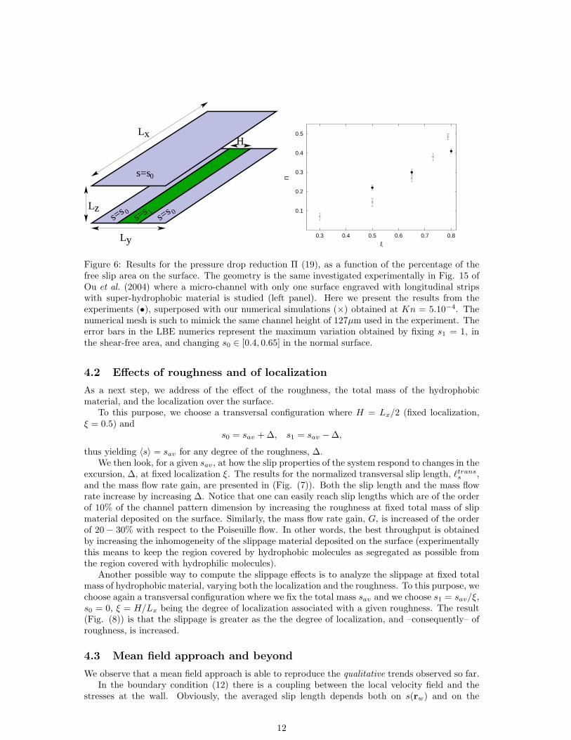
15 of Ou et al. (2004)). Here, we plot the pressure drop reduction, Π, in the microchannel as afunction of the percentage, ξ, of the free slip area on the surface (super-hydrophobic material). Wenote a remarkable agreement with the experimental results over a wide range of ξ, i.e. the ratiobetween the regions with super-hydrophobic and normal material on the wall. The geometry andKnudsen number are the same of the experiment. The only free parameters are the values of s0 ands1 assigned to the two different strips. Here, we have fixed s1 = 1 in the super-hydrophobic area,and we have varied s0 ∈ [0.4, .65] for the normal material. Notice that the LBE results exhibit thesame trend of the experiments as a function of ξ and they are even in good quantitative agreementfor ξ ∼ 0.6. Overall, there is a small dependency of Π on the unknown value of s0, at least in therange considered, as already shown by the data presented in Fig. (5). Once the correct values ofs1 and s0 able to reproduce the experimental results are identified, one may easily use the presentLBE method to predict and extend the outcomes of other experiments with different geometriesand/or distributions of the same hydrophobic material on the surface.

11

L

xL

Lz

y

H

0s=s

1s=s 0

s=s s=s0 0.1

0.2

0.3

0.4

0.5

0.3 0.4 0.5 0.6 0.7 0.8

Π

ξ

Figure 6: Results for the pressure drop reduction Π (19), as a function of the percentage of thefree slip area on the surface. The geometry is the same investigated experimentally in Fig. 15 ofOu et al. (2004) where a micro-channel with only one surface engraved with longitudinal stripswith super-hydrophobic material is studied (left panel). Here we present the results from theexperiments (•), superposed with our numerical simulations (×) obtained at Kn = 5.10−4. Thenumerical mesh is such to mimick the same channel height of 127µm used in the experiment. Theerror bars in the LBE numerics represent the maximum variation obtained by fixing s1 = 1, inthe shear-free area, and changing s0 ∈ [0.4, 0.65] in the normal surface.

4.2 Effects of roughness and of localization

As a next step, we address of the effect of the roughness, the total mass of the hydrophobicmaterial, and the localization over the surface.

To this purpose, we choose a transversal configuration where H = Lx/2 (fixed localization,ξ = 0.5) and

s0 = sav + ∆, s1 = sav − ∆,

thus yielding 〈s〉 = sav for any degree of the roughness, ∆.We then look, for a given sav, at how the slip properties of the system respond to changes in the

excursion, ∆, at fixed localization ξ. The results for the normalized transversal slip length, ℓtranss ,

and the mass flow rate gain, are presented in (Fig. (7)). Both the slip length and the mass flowrate increase by increasing ∆. Notice that one can easily reach slip lengths which are of the orderof 10% of the channel pattern dimension by increasing the roughness at fixed total mass of slipmaterial deposited on the surface. Similarly, the mass flow rate gain, G, is increased of the orderof 20 − 30% with respect to the Poiseuille flow. In other words, the best throughput is obtainedby increasing the inhomogeneity of the slippage material deposited on the surface (experimentallythis means to keep the region covered by hydrophobic molecules as segregated as possible fromthe region covered with hydrophilic molecules).

Another possible way to compute the slippage effects is to analyze the slippage at fixed totalmass of hydrophobic material, varying both the localization and the roughness. To this purpose, wechoose again a transversal configuration where we fix the total mass sav and we choose s1 = sav/ξ,s0 = 0, ξ = H/Lx being the degree of localization associated with a given roughness. The result(Fig. (8)) is that the slippage is greater as the the degree of localization, and –consequently– ofroughness, is increased.

4.3 Mean field approach and beyond

We observe that a mean field approach is able to reproduce the qualitative trends observed so far.In the boundary condition (12) there is a coupling between the local velocity field and the

stresses at the wall. Obviously, the averaged slip length depends both on s(rw) and on the

12

0.02

0.04

0.06

0.08

0.1

0.0 0.1 0.2 0.3 0.4

L s/L

x

∆

1.0

1.1

1.2

1.3

0.0 0.1 0.2 0.3 0.4G

Figure 7: Normalized transversal slip length, ℓtranss = Ls/Lx, for boundary conditions as in Fig.

(1) with s1 = sav + ∆ in a fraction ξ = H/Lx = 1/2 and s0 = sav −∆ in the other. The Knudsennumber is Kn = 0.001. We plot the normalized slip length as a function of the roughness parameter∆ and the following values of sav are considered: sav=0.4 (�), sav = 0.5 (◦), sav = 0.6 (△). Inset:Same trends of the main body but for the mass flow rate gain G.

0.01

0.03

0.05

0.07

0.09

0.2 0.3 0.4 0.5 0.6 0.7 0.8 0.9 1

L s/L

x

ξ

1.0

1.1

1.2

1.3

0.2 0.4 0.6 0.8 1.0

G

Figure 8: Normalized transversal slip length, ℓtranss = Ls/Lx, for boundary conditions of transver-

sal strips as in Fig. (1) with s1 = sav/ξ in a fraction ξ and s0 = 0 in the other. The Knudsennumber is Kn = 0.001. We plot the normalized slip length as a function of the localization pa-rameter ξ for the following values of sav: sav = 0.25 (�), sav = 0.5 (◦), sav = 0.75 (△). Inset:Same trends of the main body but for the mass flow rate gain G.

13

stresses.In order to highlight the effect of the slip function on the mean quantities, as a first approxi-

mation, we can leave the wall stress fixed at its Poiseuille value, and work only on the propertiesof s(rw), namely:

〈uslip〉 ∼ 〈s

1 − s〉. (24)

For the configuration analyzed so far, without loss of generality we define:

δ =s1 − s0

2s+ =

s0 + s1

2

and write the averaged slip properties 〈 s1−s

〉 as a function of δ and s+:

〈s

1 − s〉 = p0

s0

1 − s0+ p1

s1

1 − s1= p0

s+ − δ

1 − s+ + δ+ p1

s+ + δ

1 − s+ − δ(25)

where p1 = HLx

, p0 = 1 − p1 are the percentages of the surface associated with slip and no-slipareas respectively. Making use of Taylor expansion up to second order in δ we get:

〈s

1 − s〉 ≈

s+

1 − s++

δ

(1 − s+)2(p1 − p0) +

δ2

(1 − s+)3. (26)

Since p1 = HLx

= ξ and p0 + p1 = 1, we finally obtain:

〈s

1 − s〉 ≈

s+

1 − s++

δ(2ξ − 1)(1 − s+) + δ2

(1 − s+)3. (27)

First, in our case of a fixed localization, by setting ξ = 1/2 we have s+ = sav, δ = ∆ and weobtain:

〈s

1 − s〉 ≈

sav

1 − sav

+∆2

(1 − sav)3(28)

that results in a greater slippage when the roughness ∆ is increased.Second, if we choose s1 = sav

ξand s0 = 0, as for the case with fixed total mass, we obtain

δ = sav

2ξand s+ = sav

2ξ. This results in

〈s

1 − s〉 ≈

sav

(2ξ − sav)+

sav(4ξ2 − 2ξ)(2ξ − sav) + 2ξs2av

(2ξ − sav)3(29)

that, as a function of the localization ξ yields a qualitative agreement with our analysis, supportingthe idea that the effect of slippage is greater when slip properties are localized.

It should be appreciated that the mean field approach discussed above is not exhaustive. In fact,we can design an experiment with the boundary configuration sketched in Fig. (9), and investigatethe total slippage as a function of the distance, d, between the strips. For this geometry, the meanfield approach presented before would yield the same results irrespectively of d.

On the other hand, we expect non-linear effects to be present when the strips get close enough,due to the correlation between s(rw) and the stress at the boundary, ∂nu(rw). Indeed, as one cansee in Fig. (9), the slippage is increased when the two strips get closer to each other.

This effect, even if only of the order of 10% in the mass flow rate with respect to the con-figuration for d ≫ 1, cannot be captured by the previous mean field argument. Let us noticethat a similar sensitivity to the geometrical pattern of the slip and no-slip areas has been recentlyreported in the experimental investigation of Ou et al. (2004), where it is found that for the samemicrochannel geometries and shear-free area ratios, microridges aligned in the flow direction con-sistently outperform regular arrays of microposts. Similar considerations have been also presentedby Vinogranova (1999).

14

Lz

yL

xL

d

H

H

s=s

s=s0

1

s=s1

0s=s

s=s0

0.07

0.08

0.09

0.1

0.11

0.12

0.13

0.14

0 2 4 6 8 10

L s/L

x

d

1.25

1.35

1.45

1.55

0 2 4 6 8 10

G

Figure 9: Left: The configuration with a transversal bi-strip structure at the walls. The totalboundary lengths are Lx, Ly (stream, span). The slip coefficient is chosen as s1 = 1 in two strip oflength H and s0 = 0 in the others. The distance between the two strips is d. Periodic boundaryconditions are always assumed in the span-wise and stream-wise direction. Right: results for theslip length and the mass flow rate gain (inset) as a function of the distance d (in lattice units)between the two free-shear (s = s1) strips of width H = 20 (in lattice units). All the otherparameters, Lx = Ly = 64, Lz = 84, Kn = 1.10−3 are kept fixed.

5 Conclusions

We have presented a mesoscopic model of the fluid-wall interactions which proves capable ofreproducing some properties of flows in microchannels. We have defined a suitable implementationof the boundary conditions in a lattice version of the Boltzmann equation describing a single-phasefluid in a microchannel with heterogeneous slippage properties on the surface. In particular, wehave shown that it is sufficient to introduce a slip function, 0 ≤ s(rw) ≤ 1, defining the local degreeof slip of mesoscopic molecules at the surface, to reproduce qualitatively and, in some cases, evenquantitatively, the trends observed either in MD simulations or is some experiments. The functions(rw) plays the role of a renormalizing factor, which incorporates microscopic effects within themesoscopic description.

We have analyzed slip properties in terms of slip length, Ls, slip velocity, Vs, pressure dropgain, Π and mass flow rate Φs, as a function of the degree of slippage, and its spatial localization.The latter parameter mimicking the degree of roughness of the ultrahydrophobic material in realexperiments.

With a proper choice of the slip function s(rw) in longitudinal and transversal configurations,we have reproduced previous analytical results concerning pressure-driven hydrodynamic flowswith boundaries made up of alternating strips of zero-slip and infinite-slip (free-shear) lengths,Philip (1972a,b); Lauga & Stone (2003). We have also discussed the increment of the slip lengthin the transition regime, i.e. where the Maxwell-like slip boundary conditions (1) are supposed tobe replaced by second-order ones (2).

The local velocity profile has also been studied with changing Reynolds and Knudsen numbersand the local slip properties on the surface.

The method introduced is able to describe slip lengths of the order of the total height of thechannel (of the order of tens of µm), or fractions thereof. This is accompanied by an importantincrease in the mass flow rate, or equivalently, in the pressure drop gain. Whenever possible, wehave compared the results based on the Heterogeneous LBE with MD simulations and with somerecent experiments.

In particular, we have shown that the H-LBE approach is able to reproduce the increase ofthe slip length as a function of the inverse of the mean pressure in the channel, as observed inrecent MD simulations by Cottin-Bizonne et al. (2004). Concerning the same MD simulations,

15

6

Y

X

0

3

7 4 8

1

52 10

17 5

11

12

15

9

3

7

Z

X

Y

16

1

2

14

6

13

18

8

4

Figure 10: 2d and 3d lattice discretization of the velocities in the LBE schemes used in this work.The velocities entering in the north wall in the 2d scheme (left) are, f5, f2, f6. The outgoingvelocities are: f7, f4, f8. At the south wall the roles are exchanged.

we have found a similar linear dependency of the macroscopic slip lengths, Ls as a function ofthe microscopic slip properties at the surface. As to the experiments, we have shown that the H-LBE approach is able to achieve quantitative agreement with the experimental study presented inOu et al. (2004), concerning the slip properties as a function of the relative importance of regionswith high-slip and low-slip at the surface. The natural application of our numerical tool consistsin tuning the free parameters s0 and s1 in order to reproduce experimental results in controlledgeometries.

Then, one may use the LBE scheme with the given s0 and s1 values, to explore flows in differentgeometries and/or with different patterns of the same slip and no-slip materials.

The method is a natural candidate to study flow properties in more complex geometries, ofdirect interest for applications. Transport and mixing of active or passive quantities (macro-molecules, polymers etc...) can also be addressed.

By definition, the present H-LBE description is limited to a phenomenological interpretationof the slip function. A natural development of this approach, is to implement a multi-phaseBoltzmann description, able to attack the wall-fluid interactions and fluid-fluid interactions at amore microscopic level.

This route should open the possibility to discuss the formation of a gas phase close to the wall,induced by the microscopic details of the fluid-wall physics. Results along this direction, will makethe object of a forthcoming publication, Benzi et al. (2005).

6 Appendix A

The Lattice Boltzmann Equation (LBE) for a Pressure-driven channel flow is a streaming and col-lide equation involving the particle distribution function fl(~x, t) of finding a particle with velocity~cl (discrete velocity phase space) in ~x at time t. The equation is written in the following form:

fl(~x + ~clδt, t + δt) − fl(~x, t) = −1

τ

(

fl(~x, t) − f(eq)l (ρ, ~u)

)

+δx

c2Fgl (30)

with τ the relaxation time and gl the forcing term projection with the property∑

l

gl = 0∑

l

gl~cl = 1. (31)

For the case of two dimensional grid (2DQ9) depicted in Fig. (10), for example, the gl’s can betaken with the following properties:

g1 = −g3 g5 = g8 = −g6 = −g7 (32)

leaving only one unknown parameter, say g5. Discrete space and time increments are δx, δt, with

c = δx

δt

the intrinsic lattice velocity. The equilibrium distribution f(eq)l (ρ, ~u) is given by:

f(eq)l (ρ, ~u) = wlρ

[

1 +(~cl · ~u)

c2s

+1

2

(~cl · ~u)2

c4s

−1

2

u2

c2s

]

(33)

16

being c2s = 1

3c2 the sound speed velocity. Concerning the 2DQ9 model here used for the technicaldetails, the velocity phase space is identified by the following discrete set of velocities:

~cα =

~c0 = (0, 0)c~c1,~c2,~c3,~c4 = (1, 0)c, (0, 1)c, (−1, 0)c, (0,−1)c~c5,~c6,~c7,~c8 = (1, 1)c, (−1, 1)c, (−1,−1)c, (1,−1)c

(34)

and the equilibrium weights are w0 = 4/9, wl = 1/9 for l = 1, ..., 4, wl = 1/36 for l = 5, ..., 8.As far as the 3d model we use in the numerical analysis (3DQ19), it is a 19 velocity model whosevelocity phase space is identified by:

~cα =

~c0 = (0, 0, 0)c~c1,2,~c3,4,~c5,6 = (±1, 0, 0)c, (0,±1, 0)c, (0, 0,±1)c

~c7,...,10,~c11,...,14,~c15,...,18 = (±1,±1, 0)c, (±1, 0,±1)c, (0,±1,±1)c(35)

and equilibrium weights w0 = 1/3, wl = 1/18 for l = 1, ...6, wl = 1/36, l = 8, ..., 19.Our hydrodynamic variables such as density ρ and momentum ρu are moments of the distributionfunction fl = fl(~x, t):

ρ =∑

l

fl ρu =∑

l

~cfl (36)

and in order to derive Hydrodynamic equations from (30), we must consider the following expan-sions:

fl(~x + ~clδt, t + δt) =

∞∑

n=0

ǫn

n!Dn

t fl(~x, t) (37)

fl =∞∑

n=0

ǫnf(n)l (38)

∂t =

∞∑

n=0

ǫn∂tn(39)

where ǫ = δt and Dt = (∂t +~cl ·∇).order by order in ǫ and (30) imply: We can use the expansions

(37),(38),(39) in (30) and by equating order-by-order in ǫ self-consistent constraints on f(n)l are

obtained.Up to the first order in ǫ with ∂t = ∂t0 + ǫ∂t1 we obtain the following equations:

{

∂tρ + ∇(ρu) = 0∂tu + (u · ∇)u = − 1

ρ∇P + 1

ρ∇ · (νρ∇u)

(40)

with ν =(τ− 1

2)

3δ2

x

δt

and where ∇P contains both the imposed mean pressure drop, F, and the fluidpressure fluctuations.

7 Appendix B

Let us now go back to eq. (30), and derive explicitly the non-homogeneous boundary conditionsused in the text (12), in the limit δx = δt → 0, with c = δx

δt

→ 1. We specialize to the steady-stateboundary condition at the north-wall (z = Lz) for the 2d lattice (2DQ9):

f7(rw) = (1 − s(rw))f5(rw) + s(rw)f6(rw)

f4(rw) = f2(rw)

f8(rw) = (1 − s(rw))f6(rw) + s(rw)f5(rw).

Assuming a constant density profile ρ = 1 in the fluid, by definition we have for r = rw :

u||(rw) = f1(rw) − f3(rw) + f5(rw) − f6(rw) + f8(rw) − f7(rw). (41)

17

In the limit of small Mach numbers, disregarding all O(u2) terms in the equilibrium distributionand using the steady state, ∂tf = 0, expansion:

fl(r) =

∞∑

n=0

(−1)n(τ(cl∇))n[f(eq)l (ρ,u) + τFl] (42)

we finally obtain the estimate for the slip velocity u||:

u||(rw) = 2Fτg1 + 23u||(rw) + 2

3c2τ2∂xu||(rw)+

+2s[2Fτg5 +u||(rw)

6 − cτ6 ∂xu⊥(rw) − cτ

6 ∂yu||(rw) + c2τ2

6 (∂2x + ∂2

y)u||(rw) + c2τ2

3 ∂x∂yu||(rw)] + O(τ3).(43)

By noticing that the external forcing, F , is of the order of magnitude of the second-order stress,|∂2

yu||(rw)|ν, and ν = c2sτ , the first order in Kn of (43) reads:

u||(rw) = Kn

(

c

cs

)

s(rw)

1 − s(rw)|∂nu||(rw)| (44)

where we have used Lz∂y = ∂n , τ = LzKncs

, ∂nu||(rw) = −|∂nu||(rw)|, which is the expressionused in the text.

The second-order calculation in Kn is particularly simple if we specialize to an homogeneouscase (∂x(•) = 0). After some calculations, we obtain:

u|| = Kn

(

c

cs

)

s

1 − s|∂nu||| + Kn2

(

c

cs

)2

(1 − 4g5)|∂2nu||| (45)

which is the second order, in Kn, boundary conditions, with unknown parameters s and g5 (0 ≤g5 ≤ 1/4 ) used by Sbragaglia & Succi (2004).

References

Ansumali, S. & Karlin, I. 2002 Kinetic boundary conditions in the lattice boltzmann method.Phys. Rev E 66, 026311.

Barrat, J.-L. & Bocquet, L. 1999a Influence of wetting properties on hydrodynamic boundaryconditions at a fluid/solid interface. Faraday Discuss. 112, 119–127.

Barrat, J.-L. & Bocquet, L. 1999b Large slip effects at a nonwetting fluid solid interface.Phys. Rev. Lett. 82, 4671–4674.

Batchelor, G. 1989 An Introduction to Fluid Dynamics . Cambridge University press.

Baudry, J., Charlaix, E., Tonck, A. & Mazuyer, D. 2001 Experimental evidence for alarge slip effects at a nonwetting fluid-surface interface. Langmuir 17, 5232.

Benzi, R., Biferale, L., Sbragaglia, M., Succi, S. & Toschi, F. 2005 Mesoscopic descrip-tion of the wall-liquid interaction in microchannel flows. in preparation .

Benzi, R., Succi, S. & Vergassola, M. 1992 The lattice boltzmann equation: Theory andapplications. Phys. Rep. 222, 145.

Bhatnagar, P. L., Gross, E. & Krook, M. 1954 A model for collision process in gases. smallamplitude processes in charged and neutral one-component systems. Phys. Rev. 94, 511.

Bird, G. 1998 Direct Simulation Monte Carlo. Oxford.

Bocquet, L. & Barrat, J.-L. 1993 Hydrodynamic boundary conditions and correlation func-tions of confined fluids. Phys. Rev. Lett. 70, 2726–2729.

18

Bonnacurso, E., Butt, H. & Craig, V. 2003 Surface roughness and hydrodynamic boundaryslip of a newtonian fluid in a completely wetting system. Phys. Rev. Lett. 90, 1445011.

Bonnacurso, E., Kappl, M. & Butt, H. 2002 Hydrodynamic force measurements: Boundaryslip of water on hydrophilic surfaces and electrokinetic effects. Phys. Rev. Lett. 88, 076130.

Boon, J. & Yip, S. 1991 Molecular Hydrodynamics. Dover.

Cercignani, C. 1991 The Mathematical Theory on Non Uniform Gases: An Account of thekinetic Theory of Viscosity, Thermal Conduction and Diffusion in Gases . Cambridge UniversityPress.

Cercignani, C. & Daneri, A. 1963 Flow of rarefied gas between two parallel plates. J. Appl.Phys. 34, 3509.

Chen, S. & Doolen, G. 1998 Lattice boltzmann methods for fluid flows. Ann. Rev. Fluid Mech.30, 329.

Chen, W., Fadeev, A., Hsieh, M., Oner, D., Youngblood, J. & McCarthy, T. 1999Ultrahydrophobic and ultralyophobic surfaces: Some comments and examples. Langmuir 15,3395.

Cheng, J.-T. & Giordano, N. 2002 Fluid flow through nanometer-scale channels. Phys. Rev.E 65, 0312061.

Choi, C., K.Johan, A.Westin & Breuer, K. 2003 Apparent slip flows in hydrophilic andhydrophobic microchannels. Phys. of Fluids 15, 2897–2902.

Cieplak, M., Koplik, J. & Banavar, J. 2001 Boundary conditions at a fluid-solid interface.Phys. Rev. lett. 86, 803–806.

Cottin-Bizonne, C., Barentine, C., Charlaix, E., Bocquet, L. & Barrat, J.-L. 2004Dynamics of simple liquids at heterogeneous surfaces: Molecular dynamics simulations andhydrodynamic description. cond-mat/0404077 .

Cottin-Bizonne, C., Charlaix, E., Bocquet, L. & Barrat, J.-L. 2003 Low friction flowsof liquid at nanopatterned interfaces. Nature Materials 2, 237–240.

Craig, V., Neto, C. & Williams, D. 2001 Shear-dependent boundary slip in an aqueousnewtonian liquid. Phys. Rev. Lett. 87, 054504(1–4).

Fadeev, A. & Carthy, T. M. 1999 Trialkylsilane monolayers covalently attached to siliconsurfaces: Wettability studies indicating that molecular topography contributes to contact anglehysteresis. Langmuir 15, 3759.

Frenkel, D. & Smit, B. 1995 Understanding Molecular Simulations. From Algorithms to Ap-plications . Academic Press.

Gad-el’Hak, M. 1999 The fluid mechanics of microdevices. Fluid Eng. 121, 5–33.

Hadjiconstatinou, N. 2003 Comment on cercignani’s second-order slip coefficient. Phys. Fluids15, 2352.

Ho, C.-M. & Tai, Y.-C. 1998 Micro-electro-mechanical-systems (mems) and fluid flows. Annu.Rev. Fluid Mech. 30, 579–612.

Karlin, I., Ferrante, A. & Oettinger, H. 1999 Perfect entropy functions of the latticeboltzmann method. Europhys. Lett. 47, 182.

Karniadakis, G. & Benskok, A. 2002 MicroFlows . Springer Verlag.

19

Koplik, J. & Banavar, J. 1991 Continuum deductions from molecular hydrodynamics. Annu.Rev. Fluid Mech. 27, 257.

Kwok, D. 2003 Discrete boltzmann equation for microfluidics. Phys. Rev. Lett. 90, 1245021.

Lauga, E. & Stone, H. 2003 Effective slip in pressure-driven stokes flow. J. Fluid. Mech. 489,55.

Lim, C., Shu, C., Niu, X. & Chew, Y. 2002 Application of lattice boltzmann method tosimulate microchannel flows. Phys. fluids 14, 2299–2308.

Lion, N., Rohner, T., Arnaud, L. D. I., Damoc, E., Youhnovsky, N., Wu, Z.-Y.,

Roussel, C., Josserand, J., Jensen, H., Rossier, J., Przybylski, M. & Girault, H.

2003 Microfluidics systems in proteomics. Electrophoresis 24, 3533–3562.

Lum, K., Chandler, D. & Weeks, J. 1999 Hydrophobicity at small and large length scales. J.Phys. Chem B 103, 4570.

Massey, B. 1989 Mechanics of Fluids. Chapman and Hall.

Maurer, J., Tabeling, P., Joseph, P. & Willaime, H. 2004 Second order slip laws inmicrochannels for helium and nitrogen. Phys. Fluids 15, 2613.

Maxwell, J. 1879 On stress in rarefied gases arising from inequalities of temperature. Philos.Trans. R. Soc. 170, 231–256.

McNamara, G. & Zanetti, G. 1998 Use of the boltzmann equations to simulate lattice-gasautomata. Phys. Rev. Lett. 61, 2332.

Niu, X., Shu, C. & Chew, Y. 2004 A lattice boltzmann bgk model for simulation of micro flows.Europhys. lett. 65, 600.

Ou, J., Perot, B. & Rothstein, J. 2004 Laminar drag reduction in microchannels usingultrahydrophobic surfaces. Phys. Fluids 16, 4635.

Philip, J. 1972a Flow satisfying mixed no-slip and no-shear conditions. Z. Angew. Math. Phys.23, 353–370.

Philip, J. 1972b Integral properties of flows satisfying mixed no-slip and no-shear conditions. Z.Angew. Math. Phys. 23, 960–968.

Pit, R., Hervet, H. & Leger, L. 2000 Direct experimental evidence of slip in hexadecane:Solid interfaces. Phys. Rev. Lett. 85, 980–983.

Priezjev, N. V., Darhuber, A. & Troian, S. 2004 The slip length of sheared liquid filmssubject to mixed boundary conditions: Comparison between continuum and molecular dynamicssimulations. cond-mat/0405268 .

Rapaport, D. 1995 The Art of molecular Dynamics Simulations. Cambridge University Press .Cambridge.

Sakurai, M., Tamagawa, H., Ariga, K., Kunitake, T. & Inoue, Y. 1998 Molecular dy-namics simulation of water between hydrophobic surfaces. implications for the long range hy-drophobic force. Chem. Phys. Lett. 289, 567.

Sbragaglia, M. & Succi, S. 2004 Analytical calculation of slip flow in lattice boltzmann modelswith kinetic boundary conditions. nlin. CG/0410089 .

Schwendel, D., Hayashi, T., Dahint, R., Grunze, A. P. M., Steitz, R. & Schreiber, F.

2003 Interaction of water with self-assembled monolayers: Neutron reflectivity measurements ofthe water density in the inerface region. Langmuir 19, 2284.

20

Shan, X. & Chen, H. 1993 Lattice boltzmann model for simulating flows with multiple phasesand components. Phys. Rev E 47, 1815–1819.

Shan, X. & Chen, H. 1994 Simulation of nonideal gases and liquid-gas transitions by the latticeboltzmann equation. Phys. Rev E 47, 2941–2949.

Succi, S. 2001 The lattice Boltzmann Equation. Oxford Science.

Succi, S. 2002 Mesoscopic modeling of slip motion at fluid-solid interfaces with heterogeneouscatalysis. Phys. Rev. Lett. 89, 064502.

Swift, M., Osborn, W. & Yeomans, J. 1995 Lattice boltzmann simulations of liquid-gas andbinary fluid systems. Phys. Rev. lett. 75, 830–833.

Tabeling, P. 2003 Introduction a la microfluidique. Belin.

Thompson, P. & Robbins, M. 1989 Simulations of contact-line motion: Slip and the dynamiccontact angle. Phys. Rev. Lett. 63, 766–769.

Thompson, P. & Robbins, M. 1990 Shear flow near solids: Epiotaxial order and flow boundaryconditions. Phys. Rev. A 41, 6830–6837.

Thompson, P. & Troian, S. 1997 General boundary condition for liquid flow at solid surfaces.Nature 389, 360–362.

Toschi, F. & Succi, S. 2005 Lattice boltzmann method at finite knudsen-number. Europhys.Lett. 69, 549.

Tretheway, D. & Meinhart, C. 2002 Apparent fluid slip at hydrophobic microchannel walls.Phys. Fluids 14, L9–L12.

Tyrrell, J. & Attard, P. 2001 Images of nanobubbles on hydrophobic surfaces and theirinteractions. Phys. Rev. Lett. 87, 176104.

Verberg, R. & Ladd, A. 2000 Lattice-boltzmann model with sub-grid-scale boundary condition.Phys Rev. Lett. 84, 2148–2151.

Verberg, R., Pooley, C., Yeomans, J. & Balazs, A. 2004 Pattern formation in binaryfluids confined between rough, chemically heterogeneous surfaces. Phys. Rev. Lett. 93, 1845011.

Vinogradova, O. & Yabukov, G. 2003 Dynamic effects on force measurements. lubrificationand the atomic force microscopy. Langmuir 19, 1227.

Vinogranova, O. 1999 Slippage of water over hydrophobic surfaces. Int. J. Miner. Process. 56,31–60.

Watanabe, K., Udagawa, Y. & Ugadawa, H. 1999 Drag reduction of newtonian fluid in acircular pipe with a highly-repellent wall. J. Fluid Mech. 381, 225–238.

Whitesides, G. & Stroock, A. 2001 Flexible methods for microfluids. Phys. Today 54, 42–48.

Wolf-Gladrow, D. 2000 Lattice-Gas Cellular Automata and Lattice Boltzmann Models .Springer.

Zhang, X., Zhu, Y. & Granick, S. 2002 Hydrophobicity at a janus interface. Science 295,663–666.

Zhu, Y. & Granick, S. 2001 Rate-dependent slip of newtonian liquid at smooth surfaces. Phys.Rev. Lett. 87, 096105.

Zhu, Y. & Granick, S. 2002 Limits of the hydrodynamic no-slip boundary condition. Phys.Rev. Lett. 88, 106102.

21