ACTA UNIVERSITATIS UPSALIENSISUppsala Dissertations from the Faculty of Science and Technology

84

Karin Schönning

Meson Production in pd Collisions

Dissertation presented at Uppsala University to be publicly examined in Häggsalen, Ång-strömlaboratoriet, Lägerhyddsvägen 1, Uppsala, Friday, May 22, 2009 at 13:15 for the degree of Doctor of Philosophy. The examination will be conducted in English. Abstract Schönning, K. 2009. Meson Production in pd Collisions. Uppsala Dissertations from the Faculty of Science and Technology 84. 159 pp. Uppsala. 978-91-554-7505-5. Meson production in proton-deuteron collisions has been studied using the WASA detector facility at the CELSIUS storage ring in Uppsala. Data were obtained at two different beam energies, 1360 MeV and 1450 MeV, near the kinematic threshold for � and � mesons. The differential cross sections of pd � 3He � constitute the first measurements of this reaction covering the whole angular range. The � angular distributions are isotropic at 1360 MeV but have strong forward and backward enhancements at 1450 MeV. Theoretical calcula-tions using a two-step model fail to reproduce the shapes of the angular distributions and underestimate the total cross sections. The tensor polarisation of the � meson has been derived from the measured angular distri-butions of the � decay products. The �+�-�0 and �0� decay channels gave consistent results, showing that the � meson is produced unpolarised at both energies. This is in contrast to a recent MOMO measurement which showed that the � meson is produced almost completely polarised in the pd � 3He� reaction. Different production dynamics of � and � mesons close to threshold raises the question whether the Okubo-Zweig-Iizuka (OZI) rule is applicable in low energy nucleon-nucleon reactions. The angular distributions of the � meson produced in the pd � 3He � reaction are strongly enhanced for forward going � mesons at both energies. The �(pd � 3He �+ � - �0 )/�(pd � 3He �0 �0 �0 ) ratio has been measured and discussed in terms of isospin amplitudes. A rough estimate of the pd � 3He �0 �0 �0 �0 cross sections has also been obtained and the pd � 3He � �0 reaction has been studied for the first time near threshold. Keywords: meson production, measured angular distribution, total cross section, polarisation Karin Schönning, Division of Nuclear and Particle Physics, Box 535, Uppsala University, SE-751 21 Uppsala, Sweden © Karin Schönning 2009 ISSN 1104-2516 ISBN 978-91-554-7505-5 urn:nbn:se:uu:diva-100786 (http://urn.kb.se/resolve?urn=urn:nbn:se:uu:diva-100786) Printed in Sweden by Universitetstryckeriet, Uppsala 2009. Distributor: Uppsala University Library, Box 510, SE-751 20 Uppsala www.uu.se, acta@ub.uu.se

I systrars spårför framtids segrar

Preface

The work presented in this thesis has resulted in the following publications:

1. Polarisation of the ω meson in the pd →3 Heω at 1360 MeV and 1450MeVKarin Schönning et al., Phys. Lett. B 668 (2008) 258.

2. The pd→3 Heω reactionKarin Schönning, Kanchan P. Khemchandani et al., in the Proceedings ofthe 11th Conference on Meson-Nucleon Physics and the Structure of theNucleon (MENU 2007)SLAC eConf C070910 (2007) 282.

3. The production of ω mesons in pd→3 Heω near the kinematic thresholdKarin Schönning et al., Nucl. Phys. A 790 (2007) 319.

4. Production of ω in pd→3 Heω at CELSIUS/WASAKarin Schönning et al., in the Proceedings of the 2nd International Work-shop in η Meson physics (ETA 2007), arXiv:0710.1809v1 (2007) 99.

5. Production of ω in pd→3 Heω at kinematic thresholdKarin Schönning et al., Acta Physica Slovaca 56 (2006) 299.

Furthermore, the work has resulted in the following papers soon to bepublished:

6. Measurement of the ω meson polarization in the pd→3 Heω reaction at1360 MeV and 1450 MeV Karin Schönning et al. Accepted for publicationin Int. J. Mod. Phys. E.

7. Production of the ω meson in the pd→3 Heω reaction at 1360 MeV and1450 MeVKarin Schönning et al. Accepted for publication in Phys. Rev. C.

Two papers are also in preparation:

8. Production of the η meson and multi-pion production in pd collisions(working title)Karin Schönning et al. Foreseen submission: June 2009

9. The pd→3 Heηπ0 reaction (working title)Karin Schönning et al. Foreseen submission: August 2009

I also participated in the following publications in capacities given below:

1. Exclusive measurement of pd→3 Heππ: The ABC effect revisitedM. Bashkanov et al., Phys. Lett. B 637 223.I participated in the experimental run and in the developement of the 3Hetrigger.

2. Measurement of the η→ π+π−e+e− decay branching ratioChr. Bargholtz et al., Phys. Lett. B 644 (2007) 299.I participated in the experimental run.

3. Measurement of the slope parameter for the η → 3π0 decay in thepp→ ppη reactionM. Bashkanov et al. Phys. Rev. C 76, (2007) 048201I participated in the experimental run.

4. The pp→ ppπππ reaction channels in the threshold regionC. Pauly et al., Phys. Lett. B 649 (2007) 122I participated in the experimental run.

5. Measurement of η meson decays into lepton-antilepton pairsM. Berlowski et al., Phys. Rev. D 77 (2008) 032004I participated in the experimental run.

The following paper has recently become accepted for publication:

6. Exclusive measurement of two-pion production in the dd→4 Heππ reac-tion S.N. Keleta et al. Accepted for publication in Nucl. Phys. A.I participated in the experimental runs and in the developement of the 3Hetrigger, that was used also in the 4He case.

Contents

Preface . . . . . . . . . . . . . . . . . . . . . . . . . . . . . . . . . . . . . . . . . . . . . . . . vii1 Introduction . . . . . . . . . . . . . . . . . . . . . . . . . . . . . . . . . . . . . . . . . . 13

1.1 Quarks and Leptons . . . . . . . . . . . . . . . . . . . . . . . . . . . . . . . . . 131.2 The interactions . . . . . . . . . . . . . . . . . . . . . . . . . . . . . . . . . . . . 141.3 Brief history . . . . . . . . . . . . . . . . . . . . . . . . . . . . . . . . . . . . . . 161.4 Meson production in nucleon-nucleon collisions near threshold 20

1.4.1 Kinematical formalism . . . . . . . . . . . . . . . . . . . . . . . . . . . 211.4.2 Threshold production . . . . . . . . . . . . . . . . . . . . . . . . . . . . 22

1.5 Thesis outline . . . . . . . . . . . . . . . . . . . . . . . . . . . . . . . . . . . . . 242 Threshold production of ω mesons . . . . . . . . . . . . . . . . . . . . . . . . . 27

2.1 Experimental survey and ongoing discussions . . . . . . . . . . . . . 272.1.1 The π−p→ nω reaction . . . . . . . . . . . . . . . . . . . . . . . . . . 272.1.2 The pd→3 Heω reaction . . . . . . . . . . . . . . . . . . . . . . . . . 292.1.3 Discussion of Nimrod and SPESIV results . . . . . . . . . . . . 302.1.4 The differential cross section . . . . . . . . . . . . . . . . . . . . . . 31

2.2 Production of the ω meson in a two-step model . . . . . . . . . . . . 312.3 The OZI rule and ω production . . . . . . . . . . . . . . . . . . . . . . . . 362.4 Polarisation of the ω . . . . . . . . . . . . . . . . . . . . . . . . . . . . . . . . 382.5 Questions for this thesis . . . . . . . . . . . . . . . . . . . . . . . . . . . . . . 40

3 The CELSIUS/WASA experiment . . . . . . . . . . . . . . . . . . . . . . . . . 413.1 The CELSIUS storage ring . . . . . . . . . . . . . . . . . . . . . . . . . . . 413.2 The pellet target . . . . . . . . . . . . . . . . . . . . . . . . . . . . . . . . . . . . 413.3 The WASA detector . . . . . . . . . . . . . . . . . . . . . . . . . . . . . . . . . 44

3.3.1 The coordinate system . . . . . . . . . . . . . . . . . . . . . . . . . . . 453.3.2 The Central Detector . . . . . . . . . . . . . . . . . . . . . . . . . . . . 463.3.3 The Forward Detector . . . . . . . . . . . . . . . . . . . . . . . . . . . 503.3.4 The Tagging Spectrometer . . . . . . . . . . . . . . . . . . . . . . . . 543.3.5 The Light Pulser Monitoring System . . . . . . . . . . . . . . . . 543.3.6 The trigger and data aquisition system . . . . . . . . . . . . . . . 54

4 The 3He trigger . . . . . . . . . . . . . . . . . . . . . . . . . . . . . . . . . . . . . . . 594.1 High energy deposit in the FWC . . . . . . . . . . . . . . . . . . . . . . . 594.2 Hits in overlapping FWC and FTH elements . . . . . . . . . . . . . . 614.3 Summary of trigger conditions . . . . . . . . . . . . . . . . . . . . . . . . . 634.4 The 3He trigger performance . . . . . . . . . . . . . . . . . . . . . . . . . . 63

4.4.1 December 2004: trigger development . . . . . . . . . . . . . . . . 644.4.2 March 2005:production run . . . . . . . . . . . . . . . . . . . . . . . 65

4.4.3 May 2005:production run . . . . . . . . . . . . . . . . . . . . . . . . . 665 Calibration . . . . . . . . . . . . . . . . . . . . . . . . . . . . . . . . . . . . . . . . . . . 67

5.1 Calibration of the Forward Detector . . . . . . . . . . . . . . . . . . . . . 675.1.1 Gain correction due to count rate . . . . . . . . . . . . . . . . . . . 675.1.2 Long term time dependent corrections . . . . . . . . . . . . . . . 685.1.3 Geometrical corrections . . . . . . . . . . . . . . . . . . . . . . . . . . 695.1.4 Light quenching . . . . . . . . . . . . . . . . . . . . . . . . . . . . . . . . 695.1.5 Summary: The calibration formula . . . . . . . . . . . . . . . . . . 69

5.2 Time calibration of the plastic scintillators . . . . . . . . . . . . . . . . 705.3 Calibration of the Central Detector . . . . . . . . . . . . . . . . . . . . . . 71

5.3.1 Calibration of the Electromagnetic Calorimeter . . . . . . . . 716 Analysis . . . . . . . . . . . . . . . . . . . . . . . . . . . . . . . . . . . . . . . . . . . . . 73

6.1 Software . . . . . . . . . . . . . . . . . . . . . . . . . . . . . . . . . . . . . . . . . 736.2 Particle identification . . . . . . . . . . . . . . . . . . . . . . . . . . . . . . . . 73

6.2.1 Identification in the Forward Detector . . . . . . . . . . . . . . . 736.2.2 Identification in the Central Detector . . . . . . . . . . . . . . . . 75

7 The pd→3 Heη reaction . . . . . . . . . . . . . . . . . . . . . . . . . . . . . . . . 777.1 The phase space distribution of the 3He recoil . . . . . . . . . . . . . 777.2 Event selection . . . . . . . . . . . . . . . . . . . . . . . . . . . . . . . . . . . . 78

7.2.1 pd→ 3Heη, η→ γγ . . . . . . . . . . . . . . . . . . . . . . . . . . . . 787.2.2 pd→ 3Heη, η→ π0π0π0 . . . . . . . . . . . . . . . . . . . . . . . . . 807.2.3 pd→ 3Heη, η→ π+π−π0 . . . . . . . . . . . . . . . . . . . . . . . . 81

7.3 Consistency between decay channels . . . . . . . . . . . . . . . . . . . . 827.4 Effects from time-overlapping events . . . . . . . . . . . . . . . . . . . . 827.5 Retrieving the angular distributions . . . . . . . . . . . . . . . . . . . . . 837.6 Normalisation . . . . . . . . . . . . . . . . . . . . . . . . . . . . . . . . . . . . . 847.7 The cross sections . . . . . . . . . . . . . . . . . . . . . . . . . . . . . . . . . . 86

8 The pd→ 3Heω reaction . . . . . . . . . . . . . . . . . . . . . . . . . . . . . . . . 958.1 Event selection and acceptance . . . . . . . . . . . . . . . . . . . . . . . . 95

8.1.1 pd→ 3He ω, ω→ π+π−π0 . . . . . . . . . . . . . . . . . . . . . . . 958.1.2 pd→ 3He ω, ω→ π0γ . . . . . . . . . . . . . . . . . . . . . . . . . . 96

8.2 Sources of background . . . . . . . . . . . . . . . . . . . . . . . . . . . . . . 978.3 Results . . . . . . . . . . . . . . . . . . . . . . . . . . . . . . . . . . . . . . . . . . 98

8.3.1 Tp = 1450 MeV . . . . . . . . . . . . . . . . . . . . . . . . . . . . . . . . 998.3.2 Tp = 1360 MeV . . . . . . . . . . . . . . . . . . . . . . . . . . . . . . . . 100

8.4 The ω angular distribution . . . . . . . . . . . . . . . . . . . . . . . . . . . . 1018.4.1 Tp = 1450 MeV . . . . . . . . . . . . . . . . . . . . . . . . . . . . . . . . 1018.4.2 Tp = 1360 MeV . . . . . . . . . . . . . . . . . . . . . . . . . . . . . . . . 102

8.5 The total cross section . . . . . . . . . . . . . . . . . . . . . . . . . . . . . . . 1028.6 Data versus model calculations . . . . . . . . . . . . . . . . . . . . . . . . 1048.7 The polarisation of the ω . . . . . . . . . . . . . . . . . . . . . . . . . . . . . 105

8.7.1 The Gottfried-Jackson angle . . . . . . . . . . . . . . . . . . . . . . 1058.7.2 Event selection . . . . . . . . . . . . . . . . . . . . . . . . . . . . . . . . 1068.7.3 Results . . . . . . . . . . . . . . . . . . . . . . . . . . . . . . . . . . . . . . 107

9 Multipion production . . . . . . . . . . . . . . . . . . . . . . . . . . . . . . . . . . . 1199.1 The pd→ 3Heπ0π0π0 reaction . . . . . . . . . . . . . . . . . . . . . . . . . 1209.2 The pd→ 3Heπ+π−π0 reaction . . . . . . . . . . . . . . . . . . . . . . . . 1229.3 pd→3Heπ+π−π0 versus pd→3Heπ0π0π0 . . . . . . . . . . . . . . . 1259.4 The pd→ 3Heπ0π0 reaction . . . . . . . . . . . . . . . . . . . . . . . . . . 126

9.4.1 Event selection . . . . . . . . . . . . . . . . . . . . . . . . . . . . . . . . 1269.4.2 Sources of background . . . . . . . . . . . . . . . . . . . . . . . . . . . 1269.4.3 Results . . . . . . . . . . . . . . . . . . . . . . . . . . . . . . . . . . . . . . 127

10 The pd→ 3Heηπ0 reaction . . . . . . . . . . . . . . . . . . . . . . . . . . . . . . 12910.1 Event selection . . . . . . . . . . . . . . . . . . . . . . . . . . . . . . . . . . . . 129

10.1.1 Remark: effect from chance coincidences . . . . . . . . . . . . . 13010.2 Sources of background . . . . . . . . . . . . . . . . . . . . . . . . . . . . . . 13010.3 Results . . . . . . . . . . . . . . . . . . . . . . . . . . . . . . . . . . . . . . . . . . 130

10.3.1 Identification . . . . . . . . . . . . . . . . . . . . . . . . . . . . . . . . . . 13010.3.2 Tp = 1360 MeV . . . . . . . . . . . . . . . . . . . . . . . . . . . . . . . . 13110.3.3 Tp = 1450 MeV . . . . . . . . . . . . . . . . . . . . . . . . . . . . . . . . 131

10.4 4π0 from the pd→3Heηπ0 reaction . . . . . . . . . . . . . . . . . . . . . 13311 Summary and discussion . . . . . . . . . . . . . . . . . . . . . . . . . . . . . . . . 135

11.1 The pd→3Heη reaction . . . . . . . . . . . . . . . . . . . . . . . . . . . . . 13511.2 The pd→3Heω reaction . . . . . . . . . . . . . . . . . . . . . . . . . . . . . 13511.3 Multipion production . . . . . . . . . . . . . . . . . . . . . . . . . . . . . . . . 13711.4 The pd→3Heηπ0 reaction . . . . . . . . . . . . . . . . . . . . . . . . . . . . 138

12 Summary in Swedish:Mesonproduktion i pd-kollisioner . . . . . . . . . 13912.1 Vad är hadronfysik? . . . . . . . . . . . . . . . . . . . . . . . . . . . . . . . . 13912.2 Hur studerar vi hadronfysik? . . . . . . . . . . . . . . . . . . . . . . . . . . 14112.3 Mesonproduktion in pd-kollisioner . . . . . . . . . . . . . . . . . . . . . 142

Acknowledgement . . . . . . . . . . . . . . . . . . . . . . . . . . . . . . . . . . . . . . . . 145Appendix . . . . . . . . . . . . . . . . . . . . . . . . . . . . . . . . . . . . . . . . . . . . . . . 149Bibliography . . . . . . . . . . . . . . . . . . . . . . . . . . . . . . . . . . . . . . . . . . . . 153

1. Introduction

This thesis will deal with some aspects of the strong force and strongly inter-acting particles, i.e. hadrons. The aim is to contribute to the understandingof the reaction mechanism for meson production, in particular the ω me-son. When the first mesons were discovered in the 1940’s, they were be-lieved to be fundamental particles and the meson theories, that evolved duringthe 1930’s, were believed to describe fundamental interactions. The field ofmeson physics had a “golden era”, theoretically and experimentally, duringthe 1960’s and 1970’s. Then the quarks were discovered, Quantum Chro-modynamics (QCD) was developed as the theory of strong interactions andthe meson theories were downgraded to models. Mesons were found to becomposite systems of a quark and an anti-quark. High energy physics tookover the experimental as well as the theoretical scene and most answers weresought among fundamental particles, like quarks and gluons. The interactionsof quarks and gluons could best be studied using perturbation theory.

However, the nature of the strong force is very complex and many of its rid-dles cannot be solved in the perturbative regime. Chiral Perturbation Theoryprovided a link between the new theory of QCD and the old meson theoriesin the 1990’s and since then, one can say that the field of meson physics hasexperienced a revival.

In the following section, the reader will be briefly introduced to the fun-damental particles and the interactions between them. Focus will be on theunderstanding of the strong force. After that, we will go through the history ofmeson physics in some more detail. Then we will put this thesis into its con-text by introducing meson production in nucleon-nucleon collisions. Finally,a disposition of this thesis will be given.

1.1 Quarks and LeptonsIn Nature, there are two types of fundamental particles: quarks and leptons,summarised in table 1.1. The quarks come in six different flavours: down (d),up (u), strange (s), charm (c), bottom (b) and top (t). They all have mass,but the lightest quark (u) is around five orders of magnitude lighter than theheaviest quark (t), see table 1.1. Each quark has an antiquark partner withequal mass but opposite charge.

13

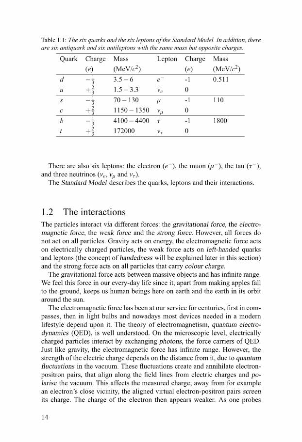
Table 1.1: The six quarks and the six leptons of the Standard Model. In addition, thereare six antiquark and six antileptons with the same mass but opposite charges.

Quark Charge Mass Lepton Charge Mass(e) (MeV/c2) (e) (MeV/c2)

d −13 3.5−6 e− -1 0.511

u +23 1.5−3.3 νe 0

s −13 70−130 μ -1 110

c +23 1150−1350 νμ 0

b −13 4100−4400 τ -1 1800

t +23 172000 ντ 0

There are also six leptons: the electron (e−), the muon (μ−), the tau (τ−),and three neutrinos (νe, νμ and ντ).

The Standard Model describes the quarks, leptons and their interactions.

1.2 The interactionsThe particles interact via different forces: the gravitational force, the electro-magnetic force, the weak force and the strong force. However, all forces donot act on all particles. Gravity acts on energy, the electromagnetic force actson electrically charged particles, the weak force acts on left-handed quarksand leptons (the concept of handedness will be explained later in this section)and the strong force acts on all particles that carry colour charge.

The gravitational force acts between massive objects and has infinite range.We feel this force in our every-day life since it, apart from making apples fallto the ground, keeps us human beings here on earth and the earth in its orbitaround the sun.

The electromagnetic force has been at our service for centuries, first in com-passes, then in light bulbs and nowadays most devices needed in a modernlifestyle depend upon it. The theory of electromagnetism, quantum electro-dynamics (QED), is well understood. On the microscopic level, electricallycharged particles interact by exchanging photons, the force carriers of QED.Just like gravity, the electromagnetic force has infinite range. However, thestrength of the electric charge depends on the distance from it, due to quantumfluctuations in the vacuum. These fluctuations create and annihilate electron-positron pairs, that align along the field lines from electric charges and po-larise the vacuum. This affects the measured charge; away from for examplean electron’s close vicinity, the aligned virtual electron-positron pairs screenits charge. The charge of the electron then appears weaker. As one probes

14

the electron, the number of electron-positron pairs decreases and so does thescreening effect. Therefore, the measured charge becomes stronger at shortdistances.

The weak force has a very short range (≈ 10−18 m or 0.1% of the diameterof a proton). As mentioned before, the weak force acts on left-handed quarksand leptons. Left-handed means that the direction of its spin axis is directedoppositely to the direction in which the particle is moving and right-handed iswhen the spin axis points in the same direction as the particle. The weak forcealso acts on right-handed anti-quarks and anti-leptons.

The force carriers are the massive W+, W− and Z bosons. Weak interac-tions can change the flavour of a quark by emitting or absorbing a W+ ora W− boson. The weak interaction can also change a particle’s parity. Elec-tromagnetism and the weak interaction are described on a common basis inelectroweak theory.

The strong force is described by the theory of quantum chromodynamics(QCD). It is rigorously and succesfully tested at short distances. According toQCD, the quarks carry colour charge and interact by exchanging gluons, theforce carriers of QCD.

However, gluons also carry colour charge and can thus interact with othergluons. This is in contrast to the force carriers of QED, i.e. the electricallyneutral photons. From QED, we learned that quantum fluctuations in the vac-uum leads to a screening effect of the electric charge. In QCD on the otherhand, the self-coupling of the gluon makes the picture quite different. Al-though screening pairs of quarks and anti-quarks create and annihilate in thevacuum, anti-screening gluons are also created.

While the strength of the measured electric charge, and hence the couplingconstant αQED, increases when the distance decreases, the strong couplingconstant αs increases when the distance increases. When the distance betweentwo colour charged particles, like a quark and an anti-quark, becomes toolarge, the interaction between them grows so strong that it takes less energyto create a new quark-antiquark pair than to separate the original quark andantiquark. Therefore, free quarks have not been observed in nature – quarksseem to appear either in quark triplets, i.e. baryons (for example the nucleon;the proton and the neutron) or in quark-antiquark pairs, i.e. mesons. Baryonsand mesons are colour neutral objects.

At sufficiently short distances, the strong coupling constant becomes small,αs � 1, and hence perturbation theory can be applied and tested with greatsuccess. At larger distances, which in particle physics is equivalent to lowerenergies of the interacting particles, the strong coupling gets larger and non-perturbative approaches, like Effective Field Theories (EFT) or Lattice QCD,have to be used. Chiral Perturbation Theory (ChPT) is an EFT where, insteadof quarks exchanging gluons, nucleons interact by exchanging mesons. Thenucleons and mesons themselves are colour neutral, but they consist of colourcharged quarks and are extended objects. At short distances, they can “sense”

15

each others colour charge. In molecular physics, there is an analogy in thevan der Waal’s force: though the atoms themselves are electrically neutral,they are extended objects made of the positively charged nucleus and the neg-atively charged electron cloud. Two atoms that are sufficiently close, senseeach other’s charge distribution and not only each others total charge. Whenthe atoms gets so close that their electron clouds overlap, the van der Waal’sforce increases and is responsible for the molecular binding by the exchangeof electrons between the atoms. The van der Waal’s force is not a fundamentalinteraction, but is an effect of electromagnetism. In the same way, the residualstrong force that leads to bound systems, i.e. nuclei, is an effect of QCD.

Chiral Perturbation Theory describes the nucleon-nucleon interaction wellup to kinetic energies of ≈100 MeV.

1.3 Brief historyThe idea of describing nuclear forces by the exchange of mesons is olderthan the idea of quarks and gluons. In this section, we will go through thediscoveries of the last century that led to the knowledge we have today.

The existence of the meson was proposed already in 1935, by the Japanesephysicist Hideki Yukawa. In his Nobel Prize winning model of the nucleon-nucleon interaction, the exchange of particles that he called mesotrons playeda crucial role. The name mesotron was later changed to the shorter meson.Yukawa’s aim was to find a potential describing the exchange particles whichmediated the nuclear force [1], in the same way as the exchange of photonsmediate to the electromagnetic force. An important difference was the range ofthe two forces; while the electromagnetic force has infinite range, the nuclearforce was known to have a range of the order of 1 fm. Yukawa discoveredthat there is a relation between the range of the interaction and the mass ofthe exchange particle. The photon, being the force carrier of an infinite rangeforce, is massless. Based on the experimentally determined range of the nu-clear force, Yukawa predicted the mass of the meson to be≈ 200 times heavierthan the electron.1

The postulated meson was found by Occhialini and Powell in 1947 [2] andis now known as the pion. Its intrinsic angular momentum, or spin, is zero.Furthermore, it has negative parity, meaning that if the spatial coordinates areinverted (x→ −x), the wave function of the pion changes sign. The spin Jand the parity P are often written as JP. The pions have JP = 0− and aretherefore pseudoscalars. Another quantity describing a hadron is its isospinT . The isospin is a fictious spin-like vector with a projection on the z-axis Tz.The isospin value T is related to the number of states n with approximatelythe same mass but different charges by n= 2 ·T+1. For example, the nucleon

1The word meson comes from “meso”, meaning “middle” and refers to that the mass waspredicted to be heavier than the electron but lighter than the proton.

16

has T = 12 and comes in an isospin doublet ; the proton and the neutron. The

projection Tz is related to the charge of the particle; the proton has Tz = +12

and the neutron Tz = −12 . In the pion case, T = 1 which means that it comes

in an isospin triplet with π+ (Tz = +1), π0 (Tz = 0) and π− (Tz = −1). Theπ+ and π− both have a mass of 139 MeV/c2 and the π0 has a mass of 135MeV/c2.

The knowledge of the pion was soon implemented in Yukawa’s theorywhich gave a refined one-pion exchange potential that was very useful in ex-plaining NN scattering data and the deuteron properties [3].

The existence of a vector meson with JP = 1− was predicted by Proca[4] already in 1936, and two years later Kemmer [5] suggested a number ofdifferent meson fields: scalar (JP = 0+), pseudoscalar (JP = 0−), axial vector(JP = 1+) and pseudo-vector (JP = 1−). Shortly after this, Wick derived therelation between the mass and the range by using Heisenberg’s uncertaintyrelation [6]. Since the exchanged particle violated the energy conservationwith ΔE = mc2, the time it is allowed to travel is given by the uncertaintyprinciple ΔEΔt= �. Then, the distance it travels with the speed of light duringthat time is R = �/mc, leading to the general rule that the range of a giveninteraction is inversely proportional to the mass of the exchange particle forthat interaction.

In 1951, Taketani, Nakamura and Sasaki (TNS) [7] suggested a division ofthe nuclear force into a long range part (r > 2fm), an intermediate range part(1fm < r < 2fm) and a short range part (r < 1fm).

One-pion exchange gives rise to the long range interaction. This was soonestablished and supported by experimental data on small angle NN-scattering[8, 9, 10, 11, 12, 13, 14].

In the intermediate range, multi-pion exchange was first suggested and suchmodels dominated during the 1950’s [15, 16]. However, the different modelsgave results that disagreed substantially with each other. They also failed toreproduce experimental data [17, 18].

In 1961, three new types of mesons were found. First, the T = 1, JP = 1−ρ meson was observed at the Cosmotron at BNL [19]. Shortly after, thediscovery of the ω meson was reported from the Lawrence RadiationLaboratory (LRL), in the invariant mass spectrum of pion triplets fromthe pp→ π+π+π−π−π0 reaction [20]. The ω meson turned out to haveT = 0, JP = 1− and a mass of ≈780 MeV. The pseudoscalar η meson(T = 0, JP = 0−) was discovered by another group at the LRL [21], inthe π+d→ ppπ+π−π0 reaction. The ω meson was also confirmed in thisexperiment.

The discovery of these heavier mesons gave rise to the one-boson exchange(OBE) model [22, 23, 24]. Now, instead of multi-pion exchange, where theinteractions between the pions were completely ignored, one assumed the ex-change of multi-pion resonances. OBE models are still successful in describ-ing the nuclear force [25, 26], but have the drawback that a scalar-isoscalar

17

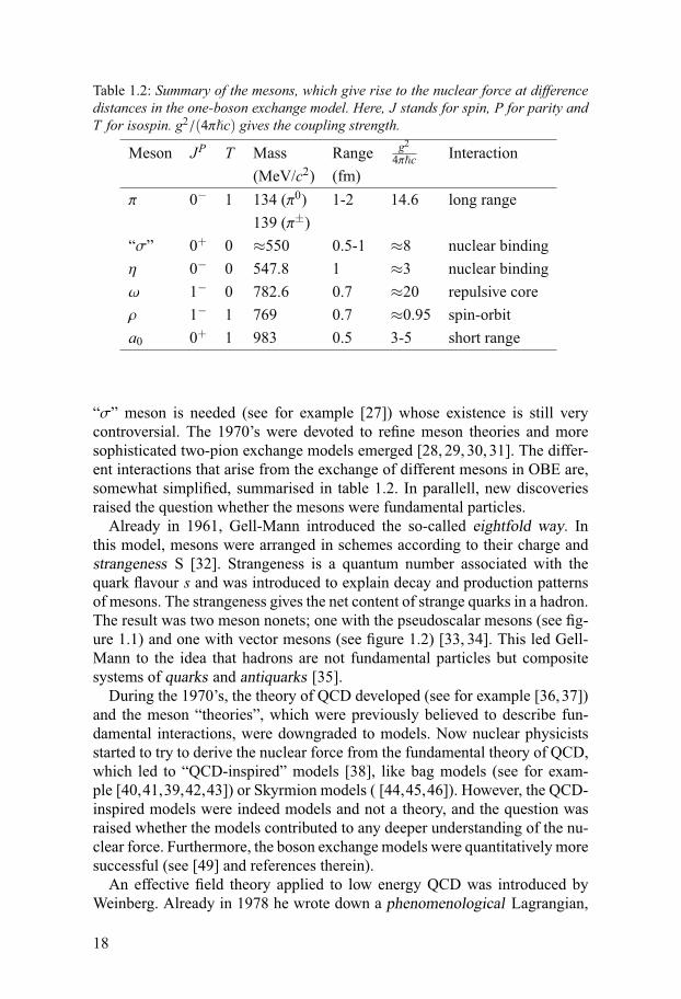
Table 1.2: Summary of the mesons, which give rise to the nuclear force at differencedistances in the one-boson exchange model. Here, J stands for spin, P for parity andT for isospin. g2/(4π�c) gives the coupling strength.

Meson JP T Mass Range g2

4π�c Interaction(MeV/c2) (fm)

π 0− 1 134 (π0) 1-2 14.6 long range139 (π±)

“σ” 0+ 0 ≈550 0.5-1 ≈8 nuclear bindingη 0− 0 547.8 1 ≈3 nuclear bindingω 1− 0 782.6 0.7 ≈20 repulsive coreρ 1− 1 769 0.7 ≈0.95 spin-orbita0 0+ 1 983 0.5 3-5 short range

“σ” meson is needed (see for example [27]) whose existence is still verycontroversial. The 1970’s were devoted to refine meson theories and moresophisticated two-pion exchange models emerged [28, 29, 30, 31]. The differ-ent interactions that arise from the exchange of different mesons in OBE are,somewhat simplified, summarised in table 1.2. In parallell, new discoveriesraised the question whether the mesons were fundamental particles.

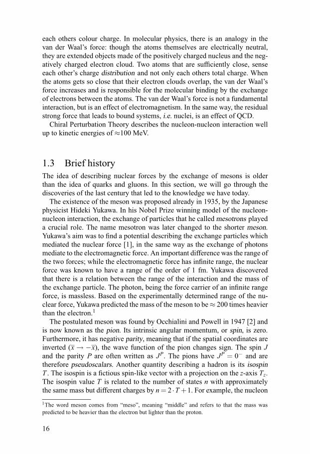
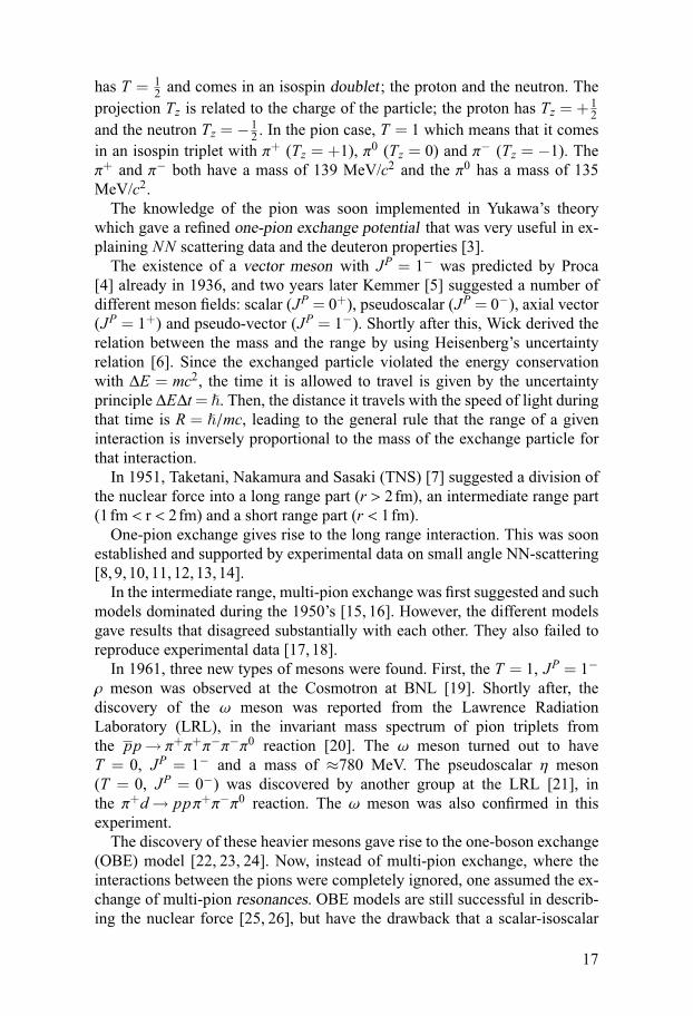
Already in 1961, Gell-Mann introduced the so-called eightfold way. Inthis model, mesons were arranged in schemes according to their charge andstrangeness S [32]. Strangeness is a quantum number associated with thequark flavour s and was introduced to explain decay and production patternsof mesons. The strangeness gives the net content of strange quarks in a hadron.The result was two meson nonets; one with the pseudoscalar mesons (see fig-ure 1.1) and one with vector mesons (see figure 1.2) [33, 34]. This led Gell-Mann to the idea that hadrons are not fundamental particles but compositesystems of quarks and antiquarks [35].

During the 1970’s, the theory of QCD developed (see for example [36,37])and the meson “theories”, which were previously believed to describe fun-damental interactions, were downgraded to models. Now nuclear physicistsstarted to try to derive the nuclear force from the fundamental theory of QCD,which led to “QCD-inspired” models [38], like bag models (see for exam-ple [40,41,39,42,43]) or Skyrmion models ( [44,45,46]). However, the QCD-inspired models were indeed models and not a theory, and the question wasraised whether the models contributed to any deeper understanding of the nu-clear force. Furthermore, the boson exchange models were quantitatively moresuccessful (see [49] and references therein).

An effective field theory applied to low energy QCD was introduced byWeinberg. Already in 1978 he wrote down a phenomenological Lagrangian,

18

K 0 K +

π− π+

K − K 0

π0η η’

Q=−1 Q=0 Q=+1

S=1

S=0

S=−1

Figure 1.1: The pseudoscalar meson nonet. Q indicates the electric charge and S thestrangeness.

K * 0 K * +

ρ− ρ+

K * − K * 0

ρ0

φ ω

Figure 1.2: The vector meson nonet. The mesons are arranged in the same was infigure 1.1 with respect to Q and S, but the vector mesons have spin 1.

i.e. its terms are derived taking as many facts about the interactions as pos-sible into account. For example, the Lagrangian must be consistent with theassummed symmetries. In this way, Weinberg obtained a description of lowenergy nucleon-nucleon interactions mediated by pion exchanges [50]. Healso pointed out that it should be possible to derive this Lagrangian from thefundamental theory of QCD. Weinberg made the pioneering step himself in1991 [51] and was soon followed by others [52, 53, 54, 55].

The central concept of the new theory, Chiral Perturbation Theory, is chiralsymmetry. This symmetry of QCD in the limit of massless quarks states thatleft-handed and right-handed particles transform independently. The chiral

19

symmetric transformation can be divided into one part that treats left-handedand right-handed particles equally, vector symmetry, and one part that treatsthem oppositely, axial symmetry.

The vector symmetry is also recognised as isospin symmetry and seemsapproximately valid in Nature; the strong interaction of the proton and itsisospin partner, i.e. the neutron, is the same. Similarly, the pions come in anisospin triplet and the strong pion-pion interaction is the same independent ofthe charge of the pion. The isospin symmetry is however only an approximatesymmetry due to the mass difference of the u and the d quark.

Axial symmetry on the other hand implies symmetry under parity rotationswhich in turn would imply parity doublets in the low-mass hadron spectrum.For example, the proton and the neutron, which have positive intrinsic parity,would have partners with equal (or at least similar) mass but negative par-ity. No such partner has been observed experimentally. This is explained bya spontaneous breaking of the axial symmetry which generates three mass-less Goldstone bosons. The Goldstone bosons are identified with the pions.Though the pions are not massless, their masses are a lot smaller than themass of any other hadron. The non-zero pion mass can be explained by thenon-zero masses of the u and d quarks (explicit breaking of the chiral symme-try).

In some sense one can claim that after more than half a century of theo-retical and experimental efforts, we are back where we started with Yukawa’smeson theory. There is one important difference though; ChPT includes chi-ral symmetry which establishes the connection with the underlying theory ofQCD.

To summarise, mesons have played and still play a crucial role in the un-derstanding of the non-perturbative regime of strong interactions.

1.4 Meson production in nucleon-nucleon collisionsnear thresholdIn the previous section, we learned that if we want to understand the stronginteraction at low energies, we have to understand the mesons and how theyinteract. An important part of hadron physics at low and intermediate energiesis therefore devoted to study the properties of the mesons, their structure andhow they interact with hadronic matter, i.e. baryons and other mesons.

Mesons can be produced by electromagnetic beams (photons, electrons,muons) or hadronic beams (pions, kaons, nucleons or nuclei), either in beam-beam collisions or in fixed-target experiments. Most mesons have relativelyshort lifetimes and decay almost immediately after being produced. Whenmesons are studied, one usually focuses either on production or on decay.

In meson decay studies, the meson in the initial state is well defined. Thismeson then decays with certain probability into different channels. It is of

20

interest to measure the probability of decay into a given channel, i.e. thebranching ratio (BR), with high precision. A specific decay channel may beforbidden if it violates some assumed symmetry. If this decay is neverthelessobserved, it indicates that this symmetry is broken to some degree.

The work in this thesis is devoted to meson production in NN collisions. Re-views summarising the field can be found in [56,57,58]. In meson productionin NN collisions, the quest is to find answers to questions like:

• How does the incident NN system interact before the production takesplace, i.e. do we understand initial state interactions (ISI)?

• How can we describe the production process? Are there several steps in-volved in the production process? If so, what mesons are involved in theintermediate steps?

• Are there any baryon resonances involved in the production process? In theenergy region discussed in this thesis, the interactions between the nucleonsare described as excitations and subsequent decays of baryon resonances.For example, the Δ(1232) and the N(1440) (Roper) resonance are impor-tant in the pion-nucleon interaction. In the η-nucleon case, the N∗(1535) isknown to play a crucial role.

• Are the final state interactions important (FSI), e.g between the nucleon-nucleon pair, between the nucleon-meson system or, if more than one me-son is produced, between the mesons?

In the case of unstable particles, final state interactions are the only possibleway to study low-energy meson-meson interactions or meson-nucleon inter-actions. Charged pions and kaons have relatively long lifetimes and at highenergies, it is possible to collect and store these mesons in a beam to inducereactions in collisions or fixed target experiments. However, neutral mesons(π0, η, ω...) are difficult to control since they do not interact electromagneti-cally and, even more importantly, their lifetimes are generally too short. Theonly option that remains is to study FSI effects in meson-nucleon or meson-meson systems. Near threshold, the final state particles have low momenta andremain close, within the range of the strong interaction, sufficiently long timeto interact with each other.

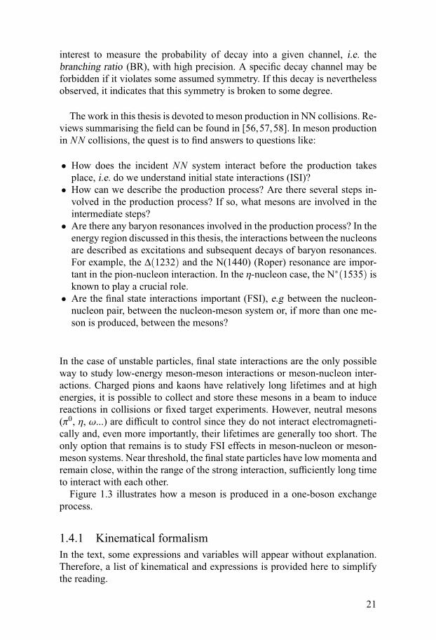
Figure 1.3 illustrates how a meson is produced in a one-boson exchangeprocess.

1.4.1 Kinematical formalismIn the text, some expressions and variables will appear without explanation.Therefore, a list of kinematical and expressions is provided here to simplifythe reading.

21

N

N

ISI FSI

π,η,ρ,ω,φ

π,η,ρ,ω,φ

N

N

Figure 1.3: A schematic diagram showing meson production in a nucleon-nucleoncollision. It includes initital state interactions (ISI), the production process (here intwo steps, represented by the circles) and final state interactions (FSI).

• CM stands for Centre of Mass. Variables in the CM system are marked witha ∗, for example p∗.

• Momentum transfer t: in a two-body reaction ab→ cd, t is given by t =(pa− pc)2 = m2

a+m2c−2papc cosθac, where θac is the angle between �pa

and �pc. Sometimes “momentum transfer” refers to the square root of themomentum transfer. This is because the square root of the momentumtransfer can be compared with particle masses. What quantity we meanin each case will be apparent from the units; if given in MeV/c, then thesquare root is referred to.

• The total energy squared s: in a reaction ab→ X, s is given bys= (pa+ pb)2.

• The excess energy Q in a reaction ab→ cd is given by Q=√s−mc−md.

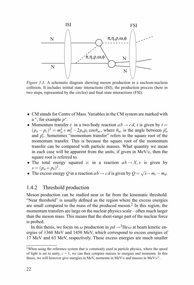
1.4.2 Threshold productionMeson production can be studied near or far from the kinematic threshold.“Near threshold” is usually defined as the region where the excess energiesare small compared to the mass of the produced meson.2 In this region, themomentum transfers are large on the nuclear physics scale – often much largerthan the meson mass. This means that the short-range part of the nuclear forceis probed.

In this thesis, we focus on ω production in pd→3Heω at beam kinetic en-ergies of 1360 MeV and 1450 MeV, which correspond to excess energies of17 MeV and 63 MeV, respectively. These excess energies are much smaller

2When using the reference system that is commonly used in particle physics, where the speedof light is set to unity, c = 1, we can then compare masses to energies and momenta. In thisthesis, we will however give energies in MeV, momenta in MeV/c and masses in MeV/c2.

22

than the ω mass, 782.6 MeV/c2. The minimum momentum transfer, whichoccurs for forward going ω mesons, is ≈1110 MeV/c and ≈935 MeV/c, re-spectively. A measurement of the differential cross section as a function of theω production angle in the CM system, θ∗ω, gives important input to the intrigu-ing question how mesons are produced in few body collisions. We compareour results to calculations using a sequential two-step model. The calculationshave been carried out by K.P. Khemchandani and will be further explained inthe following chapter. Furthermore, a measurement of the tensor polarisationof the ω meson makes it possible to compare the ω meson with its SU(3) sin-glet partner, the φ meson. A comparison gives information on the productionmechanism.

In addition to ω production, data extracted from other pd→3HeX reactionsare analysed: η production at slightly higher excess energies than in the ωcase, multipion production well above threshold and finally ηπ0 productionnear threshold.

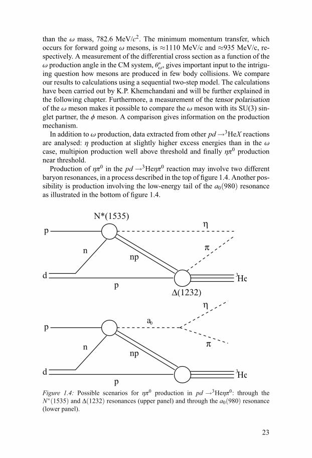
Production of ηπ0 in the pd→3Heηπ0 reaction may involve two differentbaryon resonances, in a process described in the top of figure 1.4. Another pos-sibility is production involving the low-energy tail of the a0(980) resonanceas illustrated in the bottom of figure 1.4.

npn

p

η

π

N*(1535)

Δ(1232)

3He

p

d

npn

p3He

p

d

π

η

0a

Figure 1.4: Possible scenarios for ηπ0 production in pd →3Heηπ0: through theN∗(1535) and Δ(1232) resonances (upper panel) and through the a0(980) resonance(lower panel).

23

1.5 Thesis outlineThis is a thesis in experimental hadron physics. The data have been collectedat the The Svedberg Laboratory by the CELSIUS/WASA collaboration. Theexperimental equipment has been planned, built, developed and tested by alarge number of people. The author of this thesis has participated in the plan-ning of the runs where the thesis data were collected, in particular the triggersimulations and trigger testing. The author also participated in the data taking,together with the other collaborators.

The main work done by the author are simulations and offline analysis ofexperimental data. The calibration was performed together with Jozef Zło-manczuk who also developed the major part of the software being used. Theanalysis of the different reactions presented here was performed by the au-thor. The two-step model calculations were performed by Kanchan P. Khem-chandani in continous discussions with the author. The interpretation of thepolarisation results was made in discussions between the author and ColinWilkin. Chapter 1, 2, 3 and 6 describe work, theoretical as well as experimen-tal, made by others. In chapter 4, several people were involved in the preparingdiscussions, contributing with ideas: Jozef Złomanczuk, Kjell Fransson, PiaThörngren-Engblom, Samson Negasi Keleta and the author. The simulationsand the offline analysis part were performed by the author while the hardwaretrigger developement was done by Kjell Fransson and Pawel Marciniewski.The methods in chapter 5 were implemented and developed by Jozef Zło-mancuk in discussions with the author who tested and used the tools. All theanalyses in chapters 7-10 were performed by the author and in chapter 11 theresults are summarised.A more detailed description of the thesis disposition is given as follows:Chapter 2: Threshold production of ω mesonsThe reader will here be introduced to the ω-related physics first by a surveyof earlier measurements of ω production, followed by a short summary ofthe theoretical work. Then we will proceed by describing meson productionwithin a two-step model that has been used in the calculations which our datahave been compared with. Finally the OZI rule will be introduced and we willdescribe how it is related to our measurements of the ω tensor polarisation.Chapter 3: The CELSIUS/WASA experimentThe experimental setup will be presented: the CELSIUS storage ring, the pel-let target, the WASA detector with all its subdetectors and the trigger andaquisition system.Chapter 4: The 3He triggerA special trigger was developed for selection of 3He events. In this chapter,the basic principles of the trigger are presented and its performance is investi-gated.Chapter 5: CalibrationThe calibration procedure is here explained. The WASA Forward Detector

24

is at focus and several effects are parametrised and included: gain drift dueto count rate, long term gain instabilities, geometrical corrections and lightquenching.Chapter 6: AnalysisThe analysis tools, i.e. the software packages that describe hadronic kinemat-ics and interactions within the detector setup used in this thesis, are brieflypresented. The particle identification procedure is also explained.Chapter 7: The pd→3Heη reactionThe behaviour of the pd →3Heη reaction is well known; this gives the op-portunity to study the detector and reconstruction performance by comparingWASA results to older data from other experiments. Furthermore, three dif-ferent decay channels of the η are compared. The η→ γγ channel is almostbackground free and has been used for calculating the luminosity. The dif-ferential cross section as a function of cosθ∗η has been measured in a largerangular range than previous measurements at this energy.Chapter 8: The pd→3Heω reactionIn this chapter, the ω measurements are presented in detail. The differentialcross section as a function of cosθ∗ω has been studied and the total cross sec-tion was measured. The results were compared to model calculations. Fur-thermore, a measurement of the tensor polarisation of the ω was obtained bystudying the angular distribution of its decay products.Chapter 9: Multipion productionMultipion production constitute the most important background to the mesonchannels studied in this thesis. This chapter describes the measurements of thetotal cross section of pd→3Heπ+π−π0, pd→3Heπ0π0π0 and pd→3Heπ0π0.We also give rough estimates of the pd→3Heπ0π0π0π0 cross section.Chapter 10: The pd→3Heηπ0 reactionThe total cross sections of ηπ0 production in pd→3Heηπ0 has been measuredat both energies and the results are given here.Chapter 11: Summary and discussionChapter 11 summarises the thesis with conclusions drawn and points towardsopen questions.Chapter 12: Summary in SwedishA popularised version of the summary is given here, in swedish.

25

2. Threshold production of ω mesons

In the following, an introduction to physics related to the ω meson is given.The chapter starts with a review of previous measurements of ω meson pro-duction and proceeds by presenting the basic principles of a model describ-ing meson production at large momentum transfers. Then, ω production isdiscussed within the OZI context. Finally, we will introduce some conceptsrelated to polarisation and explain how the ω polarisation can be measured.

2.1 Experimental survey and ongoing discussionsThe production of ω mesons near the kinematic threshold has been studiedat several facilities. Three extensive studies were performed at the Nimrodsynchrotron at the Rutherford Laboratory in the 1970’s, where the ω mesonswere produced in the π−p→ nω reaction [59, 60, 61]. During the same era,ω production was studied for the first time in the pd →3 Heω reaction atthe Princeton-Pennsylvania Accelerator [62], at energies well above thresh-old. Around 20 years later, measurements of the pd→3 Heω reaction wereperformed with the SPESIV spectrometer [63, 64] at SATURNE. These mea-surements are of particular interest here and their findings will therefore besummarised in section 2.1.2. The interpretation of the Nimrod data as wellas the SPESIV data have been object of some criticism [65, 66] which willbe discussed in section 2.1.3. Finally the only previous measurement of theangular distribution of the ω in pd→3 Heω [67], obtained with the SPESIIIspectrometer at SATURNE, will be presented.

2.1.1 The π−p→ nω reactionIn the early 1970’s, measurements of η, ω, φ and η′ production in π−p→ nX0

were carried out at the Nimrod synchrotron at the Rutherford Laboratory byBinnie et al. [59].

In this experiment, pions with a well defined momentum were brought intocollision with a hydrogen target. The neutron momenta were determined bya time-of-flight-technique. Furthermore, charged particles were detected inscintillator strips and photons in γ-detectors. In this way, different final statescould be separated.

27

The η, ω, φ and η′ mesons were identified by the missing mass technique,meaning that in the missing mass spectrum of the recoil particle, the mesonsappear in peaks at their nominal masses. This technique is common and hasbeen used also in this thesis. However, instead of reconstructing the missingmass keeping the incident pion momentum k fixed and scan over the measuredkinematic variables in the final state (like the neutron momentum p and theneutron emission angle θ), the spectra were obtained by varying the incidentmomentum across the production threshold while the final state variables wereheld constant within a small range. In [59], this is referred to as the threshold-crossing technique.

In production of a particle in a two-body reaction, the total cross sectionσ isrelated to the differential cross section with respect to the momentum transfert by σ = 4p∗k∗dσ/dt, where k∗ is the incident momentum in the CM systemand p∗ the outgoing momentum in the CM system. In the Nimrod experiment,the variation in k∗ is very small and in s-wave production, dσ/dt is constant.Then the total cross section should be proportional to p∗, σ ∝ p∗.

The φ and η′ mesons were found to be produced in a way consistent with s-wave production, with a cross section that was proportional to p∗. A forward-backward asymmetry in the angular distribution was observed in the η case;this was explained by a p-wave contribution. However, theωmeson, measuredin the region ranged from p∗ω ≈ 40 MeV/c up to about 200 MeV/c, showed asurprising threshold behaviour. The total cross section was significantly sup-pressed for p∗ω < 80 MeV/c. In this region, the cross section was rather givenby σ ∝ p∗2.

However, Binnie et al. still suggested that s-wave production is most likelyfor the ω since they observed forward-backward symmetry also in ω produc-tion. Besides, Abolins et al. [69] had measured the differential cross sectionearlier well above the threshold region (at p∗ω = 260 MeV/c) and found noevidence of higher partial waves.

The reason for the threshold suppression was believed to be due to rescat-tering; if the ω meson decays sufficiently soon after its production, one of thedecay pions can interact with the neutron which could then be scattered in acompletely different direction and escape detection. This could influence theneutron count rate and, if the effect is not corrected for, also the measuredcross section.

The measurements of ω production in π−p → nω were repeated a fewyears later by Keyne et al. using essentially the same equipment, thoughslightly extended to get even closer to the production threshold; the rangewas 20 MeV/c < p∗ω < 260 MeV/c this time. Furthermore, the statisticalprecision was higher.

Keyne et al. could confirm the drop in the cross section near threshold, butthe explanation that it would be due to neutron-pion rescattering was aban-doned for two reasons: First, the rescattering effect would be stronger in theω→ π+π−π0 decay channel (BR=89.1%) than in the ω→ π0γ decay channel

28

(BR=8.7%). The cross section calculated from the ω→ π+π−π0 decay chan-nel would then appear smaller than the one obtained in the ω→ π0γ case.The measured branching ratio, given by the measured count rate of a givendecay channel divided by the total count rate of ω events, would then have ap∗ω dependent behaviour.

However, both decay channels were studied and the measured branchingratio was found to be remarkably constant in p∗ω.

Second, rescattering off the neutron would distort the neutron distribution.Either the rescattering changes the neutron momentum completely causing itto escape detection, which could give the scenario just described, or it couldbe modestly distorted causing a broader ω peak in the missing mass spectrum.However, the measured width of the ω peak was constant for all p∗ω. An ex-planation with the effect of two N∗ resonances, S 11(1650) and P11(1710) wasshown to be consistent with the p∗ω dependence near threshold and with anisotropic angular distribution.

A third Nimrod measurement by Karami et al. [61], covering the full θ∗ωrange, confirmed both isotropy in dσ/dΩ∗ω and the threshold drop of the crosssection.

Again, a combination of s- and p-waves in the production was suggestedwhich reproduced the momentum and angular dependence. Elastic π−p scat-tering data were analysed in the same work to see if effects of unitarity re-sulting from the opening of the ωn channel could be observed. However, themodel suggested by Keyne et al. did not seem to be consistent with the ob-served effects in the elastic channel.

It should be pointed out that the reported threshold behaviour of theπ−p→ nω is said to be unexpected with respect to s-wave production, butif all partial waves up to l = 3 are included, which was done by the Giessentheory group [68], the threshold behaviour of the total cross section and theisotropic angular distributions are reproduced fairly well.

2.1.2 The pd→3 Heω reactionIn the middle 1970’s at the Princeton-Pennsylvania Accelerator, Brody et al.studied meson production in the pd→3 HeX0 reaction, but the energies werewell above the kinematic threshold.

Fourteen years later, Plouin et al. studied the threshold excitation curve withthe SPESIV spectrometer [73] at the Saturne II synchrotron of the LaboratoireNational Saturne. This did, however, only lead to preliminary results [63].

Inspired by this and by the work of the Nimrod group ( [59, 60, 61]),Wurzinger et al. [64] explored the threshold region in pd → 3Heω usingthe same apparatus as Plouin et al.. A proton beam was focused on a LD2target and the 3He ions were separated from the beam protons by a dipolemagnet. The 3He ions were then identified in two scintillator hodoscopes thatalso measured their time-of-flight. Two multi-wire drift chambers allowed

29

tracking of the 3He ions back to the target location. No decay products weremeasured.

The differential cross section dσ/dΩ∗ at θ∗ω = 180o was measured for 21different values of p∗ω. Far away from threshold, the SPESIV spectrometer wastuned to be sensistive to backscattered ω at the nominal mass value. Close tothreshold, they used the same threshold-crossing technique as described byBinnie et al. [59]. The averaged square amplitude, | fω|2, defined as

| fω|2 =p∗pp∗ω

(dσdΩ∗

)180o (2.1)

was calculated and a suppression near threshold was observed, similar to whatwas seen by the Nimrod group [59, 60, 61]. The solution suggested by Keyneet al. [60], where the threshold suppression is caused by a S 11(1650) and aP11(1710) resonance excitation, was not considered by the authors of [64].They expected the coupling of the P11(1710) to ωN to be small since its cou-pling to γN is small. Furthermore, they considered the two-resonance picturefrom a πN system to be unlikely to stay intact in a pd system.

Instead, the rescattering effect discussed by Binnie et al. and Keyne et al.was reconsidered. When rescattering of the decay pions was taken into ac-count in a classical Monte Carlo model, the simulations of the ω→ π+π−π0

channel was shown to reproduce the threshold suppression fairly well. How-ever, since no other final state particle than the 3He was detected, the decaychannels could not be separated and Wurzinger et al. did not draw any quan-titative conclusions.

In a follow-up paper by the same group [70], the authors mention in a foot-note that a mistake had been made in the normalisation of the Jacobian in theanalysis that lead to the results in [64], causing the averaged squared ampli-tude near threshold given therein to be underestimated by a factor of 2.

2.1.3 Discussion of Nimrod and SPESIV resultsThe interpretation of the Nimrod and the SPESIV measurements have beenobjected to criticism. Hanhart and Kudryavtsev argue in [65] that the data in-terpretation in [59, 60, 61, 64] is incorrect. When using the threshold-crossingtechnique, the differential cross section is obtained by integrating over thebeam momentum. However, as outlined in [65], the Nimrod as well as theSPESIV group performed the integration using a δ-function describing theconservation of energy. For a resonance with a finite width Γ the spectral den-sity ρ(m,Γ) should be used instead. Hanhart and Kudryavtsev conclude thatonly when

2P∗ΔPμΓ

� 1 (2.2)

30

is fulfilled (μ being the reduced mass of the meson and the neutron in theNimrod case, ΔP the resolution of the neutron momentum and P∗ the CMmomentum of the neutron), the reaction rate behaves like a simple two-bodycross section with stable particles involved.

Hanhart, Sibirtsev and Speth brought up the discussion again and recalcu-lated the cross section assuming that the formalism in [59] was applied im-properly [66]. Under this assumption, the threshold suppression of the crosssection is a kinematical effect and after correcting for it, the authors of [66]concluded that the unexpected momentum dependence near threshold is re-moved. Also in [71], the Nimrod data from Karami et al. were re-analysed bySibirtsev and Cassing.

Neither Ref. [65] or [66] suggest any explanation on why the φ measure-ments in from Binnie et al. [59] showed no threshold suppression similar tothe one observed in the ω case. The φ meson has a width of 4.26 MeV, com-parable to ω width of 8.44 MeV/c2. The condition given in equation 2.2 wasnot fulfilled in the φ case near threshold in the measurements by Binnie etal. A threshold suppression also in φ production would have been observed,provided Hanhart, Kudryavtsev, Sibirtsev and Speth are right. However, nodeviation from s-wave production was found in the φ case.

Penner and Mosel [72] replied with criticism of the conclusions in [65]and [66] and support the data interpretation by Nimrod and SPESIV groups[59, 60, 61, 64], but it is to this day not clear who is right. To bring clarity intothe issue, more data on ω production are needed. This thesis will hopefully beone step on the way.

2.1.4 The differential cross sectionThe until now only data on the angular distribution, dσ/dΩ∗ω, of ω mesonsfrom pd →3Heω were provided by Kirchner et al. with the SPESIII spec-trometer [67]. They measured the differential cross section at twelve differentcosθ∗ω ponts at a beam energy of Tp = 1450 MeV. They observed a clearanisotropy with a very sharply rising differential cross section for forward go-ing ω mesons (see figure 2.1), which can be interpreted as if higher partialwaves participate in the production process. However, the SPESIII spectrom-eter did not cover the region -0.4 < cosθ∗ω < 0.8 and no attempt was made toexplain the sharp forward peak. Until now, no further measurements on thedifferential cross section have been made.

2.2 Production of the ω meson in a two-step modelMeson production in pd collisions can be modeled in different ways. The sim-plest models describe direct production and involves one (one-body mecha-nism) or two (two-body mechanism) of the three nucleons. In the one-body

31

Figure 2.1: SPESIII pd→3Heω data taken at a beam energy of Tp = 1450 MeV [67].

mechanism, one nucleon is active, either the beam proton or the target protonor neutron within the deuteron, while the remaining two are spectators. Detailscan be found in [74]. Laget and Lecolley found that the one-body mechanismin pd reactions is strongly supressed in π production and even more in η pro-duction [75]. In the two-body mechanism, two nucleons interact and producea meson while the third nucleon remains a spectator. This model was used byLaget and Lecolley to explain pion production in pd collisions [74]. In theω case, the ω meson would be produced in for example a pp→ ppω or apn→ dω subprocess. At the beam energies 1360 MeV and 1450 MeV, thesereactions are below threshold, but they can occur thanks to the Fermi motionof the nucleons within the target deuteron. However, it was found in [74] thatthe two-body mechanism is unable to reproduce data from reactions with highmomentum transfers [76].

To handle large momentum transfers, three-body mechanisms are needed.All three nucleons then participate in the production mechanism, which isdivided into two steps. Therefore it will here be referred to as the two-stepmodel.

The two-step model was first suggested by Kilian and Nann [77] in orderto handle the large momentum transfer in heavy meson production. As men-tioned in section 1.4, the minimum momentum transfer in pd→3Heω at 1360MeV is as large as 1110 MeV/c and 935 MeV/c at 1450 MeV. The two-stepmechanism implies sharing of the momentum transfer between the three nu-cleons. Figure 2.2 illustrates schematically the two-step model. In the firststep, the beam proton interacts with a proton (neutron) in the deuteron and

32

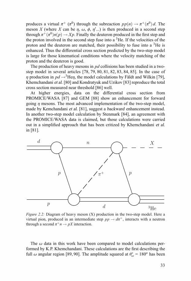
produces a virtual π+ (π0) through the subreaction pp(n) → π+(π0)d. Themeson X (where X can be η, ω, φ, η′...) is then produced in a second stepthrough π+(π0)n(p)→ Xp. Finally the deuteron produced in the first step andthe proton involved in the second step fuse into a 3He. If the velocities of theproton and the deuteron are matched, their possibility to fuse into a 3He isenhanced. Thus the differential cross section predicted by the two-step modelis large for those kinematical conditions where the velocity matching of theproton and the deuteron is good.

The production of heavy mesons in pd collisions has been studied in a two-step model in several articles [78, 79, 80, 81, 82, 83, 84, 85]. In the case ofη production in pd→3Heη, the model calculations by Fäldt and Wilkin [79],Khemchandani et al. [80] and Kondratyuk and Uzikov [83] reproduce the totalcross section measured near threshold [86] well.

At higher energies, data on the differential cross section fromPROMICE/WASA [87] and GEM [88] show an enhancement for forwardgoing η mesons. The most advanced implementation of the two-step model,made by Kemchandani et al. [81], suggest a backward enhancement instead.In another two-step model calculation by Stenmark [84], an agreement withthe PROMICE/WASA data is claimed, but those calculations were carriedout in a simplified approach that has been critized by Khemchandani et al.in [81].

����

����

����

����

����������

p

��

��

��

��

��

p

n

p

X

��

��

��

��

��

��

��

π+

3He

d

d

Figure 2.2: Diagram of heavy meson (X) production in the two-step model. Here avirtual pion, produced in an intermediate step pp→ dπ+, interacts with a neutronthrough a second π+n→ pX interaction.

The ω data in this work have been compared to model calculations per-formed by K.P. Khemchandani. These calculations are the first describing thefull ω angular region [89, 90]. The amplitude squared at θ∗ω = 180o has been

33

calculated before by Kondratyuk and Uzikov in [83] and the results reproducethe threshold behaviour observed by Wurzinger et al. in [64], but the crosssections obtained were nearly an order of magnitude smaller than those fromexperiment. The Khemchandani implementation of the model presented hereis similar to that of [83] with a T-matrix that can be written as:

〈 |Tpd→3Heω | 〉 = i32d �P1(2π)3

d �P2(2π)3 ∑

intm′s〈 pn|d 〉〈π+d |Tpp→πd | pp〉 (2.3)

1K2π−m2

π+ iε〈ωp |Tπn→ωp |π+n〉〈3He | pd 〉,

where �P1 is the Fermi momentum of the initial proton and the neutron insidethe target deuteron in the deuteron CM system and �P2 the momentum of the fi-nal proton and deuteron, in the rest system of the 3He. Kπ is the momentum ofthe intermediate pion in the π−N CM system. For some textbooks describingthe formalism of T-matrices etc., see for example [91] or [92].

The work then follows closely the approach described in [80] for η produc-tion and is summarised in [89, 90]:• The pp→ πd vertex is written in terms of a parameterised T-matrix [93].• The deuteron wave function is written in terms of the Paris potential [94].• For the 〈3He | pd 〉 overlap function, the parametrisation from [95] is used.• The π+(π0)n(p)→ pω subprocess is the main difference between the cal-

culations by Khemchandani and those of Kondratyuk and Uzikov [83].Kondratyuk and Uzikov used experimental data divided by phase space.Khemchandani has evaluated it using the Giessen model [68], which is aneffective Lagrangian approach that takes a large set of differential and totalcross sections for seven coupled channels into account; γN, πN, 2πN, ηN,ωN, KΛ and KΣ.

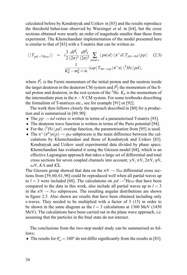
The Giessen group showed that data on the πN → Nω differential cross sec-tions from [59,60,61,96] could be reproduced well when all partial waves upto l = 3 were included [68]. The calculations on pd→3Heω that have beencompared to the data in this work, also include all partial waves up to l = 3in the πN → Nω subprocess. The resulting angular distributions are shownin figure 2.3. Also shown are results that have been obtained including onlys-waves. They needed to be multiplied with a factor of 3 (15) in order tobe shown in the same diagram as the l = 3 calculations at 1360 MeV (1450MeV). The calculations have been carried out in the plane wave approach, i.e.assuming that the particles in the final state do not interact.

The conclusions from the two-step model study can be summarised as fol-lows:• The results for θ∗ω = 180o do not differ significantly from the results in [83].

34

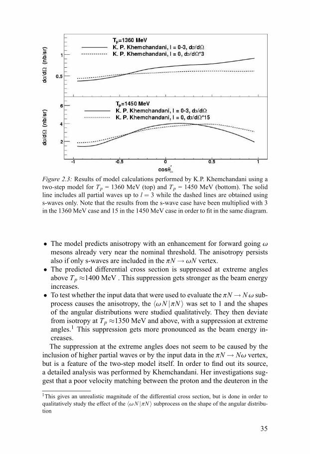
Figure 2.3: Results of model calculations performed by K.P. Khemchandani using atwo-step model for Tp = 1360 MeV (top) and Tp = 1450 MeV (bottom). The solidline includes all partial waves up to l = 3 while the dashed lines are obtained usings-waves only. Note that the results from the s-wave case have been multiplied with 3in the 1360 MeV case and 15 in the 1450 MeV case in order to fit in the same diagram.

• The model predicts anisotropy with an enhancement for forward going ωmesons already very near the nominal threshold. The anisotropy persistsalso if only s-waves are included in the πN→ ωN vertex.

• The predicted differential cross section is suppressed at extreme anglesabove Tp ≈1400 MeV . This suppression gets stronger as the beam energyincreases.

• To test whether the input data that were used to evaluate the πN→ Nω sub-process causes the anisotropy, the 〈ωN |πN 〉 was set to 1 and the shapesof the angular distributions were studied qualitatively. They then deviatefrom isotropy at Tp ≈1350 MeV and above, with a suppression at extremeangles.1 This suppression gets more pronounced as the beam energy in-creases.The suppression at the extreme angles does not seem to be caused by the

inclusion of higher partial waves or by the input data in the πN→ Nω vertex,but is a feature of the two-step model itself. In order to find out its source,a detailed analysis was performed by Khemchandani. Her investigations sug-gest that a poor velocity matching between the proton and the deuteron in the

1This gives an unrealistic magnitude of the differential cross section, but is done in order toqualitatively study the effect of the 〈ωN |πN 〉 subprocess on the shape of the angular distribu-tion

35

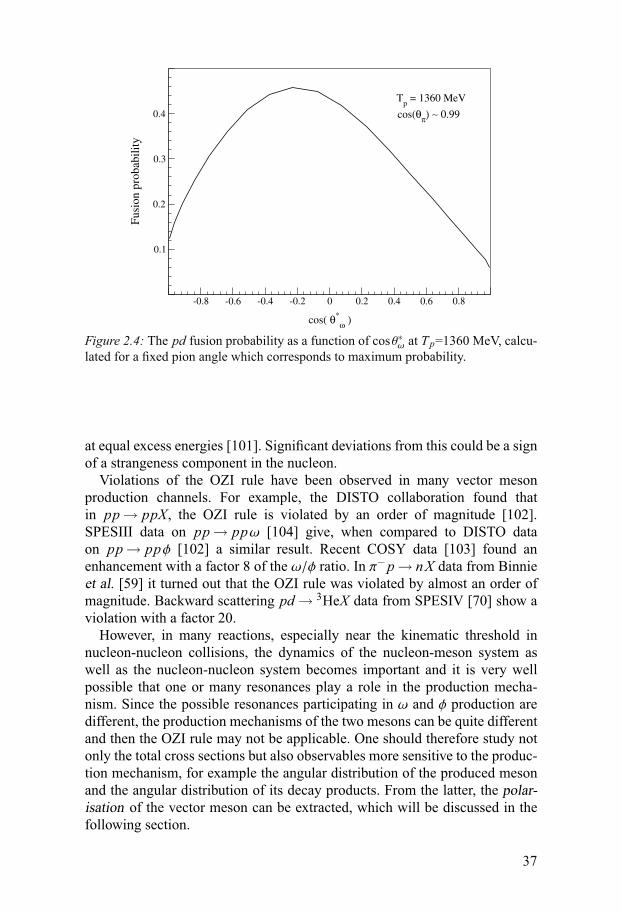
〈3He|pd〉 overlap function occurs at extreme angles. The effect is enhancedas the beam energy increases. Figure 2.4 and 2.5 shows the probablity of pdfusion into 3He as a function of cosθ∗ω. By following [77], the probability isobtained for this specific channel as

p= exp(−√s−mp−mdEb

), (2.4)

where√s is the total energy of the pd pair in the final step, mp, md and Eb are

the total energy, the proton mass, the deuteron mass and the binding energy ofa proton and a deuteron in 3He, respectively (Eb = 5.49 MeV). When studyingthe velocity matching, the Fermi momentum of the proton and the neutron inthe target deuteron was set to an average value of 100 MeV/c. Furthermore,their polar and azimuthal angles were fixed to zero and the intermediate pion isassumed to move in the forward direction only. These restriction on the pionwas made in order to give the best velocity matching conditions and werenot applied in the model calculations predicting the angular distributions andtotal cross sections. It should also be mentioned that the findings presentedhere hold qualitatively also when the intermediate pion is produced at otherangles. The probability distribution at 1360 MeV, shown in figure 2.4, hasdips at extreme angles but never gets smaller than ≈7%. Consequently thedifferential cross section predicted at this energy is closer to isotropy thanat 1450 MeV, where the probability of velocity matching almost vanishes ascosθ∗ω approaches 1 or -1 (see figure 2.5). The two-step model thus predict asuppressed cross section at small and large angles. One of the questions askedin this thesis is whether the experimental data agree with the two-step model.

2.3 The OZI rule and ω productionThe production ofω and the other light isoscalar vector meson, the φ, are oftencompared within the framework of the Okubo-Zweig-Iizuka rule (OZI) [97,98,99]. The OZI rule states that all processes with disconnected quark lines areforbidden. If the φ meson, as described within the naïve quark model, wouldhave been an ideally mixed ss state, φ production in nucleon-nucleon inter-actions is forbidden by the OZI rule. However, φ can occur via a strangenesscomponent within the nucleon or via the deviation from ideal mixing. The φmeson deviates from ideal mixing with δV = 3.7o [100].

The suppression of φ production compared to ω production in the reactionAB→ (φ/ω)X, where A, B and X stands for hadronic systems consisting oflight quarks only, should quantitatively be

RAB =σ(AB→ Xφ)σ(AB→ Xω)

= tan2(δV)≈ 4.2 ·10−3 (2.5)

36

-0.8 -0.6 -0.4 -0.2 0 0.2 0.4 0.6 0.8

cos( θ∗ω )

0.1

0.2

0.3

0.4

Fusi

on p

roba

bilit

y

Tp = 1360 MeV

cos(θπ) ∼ 0.99

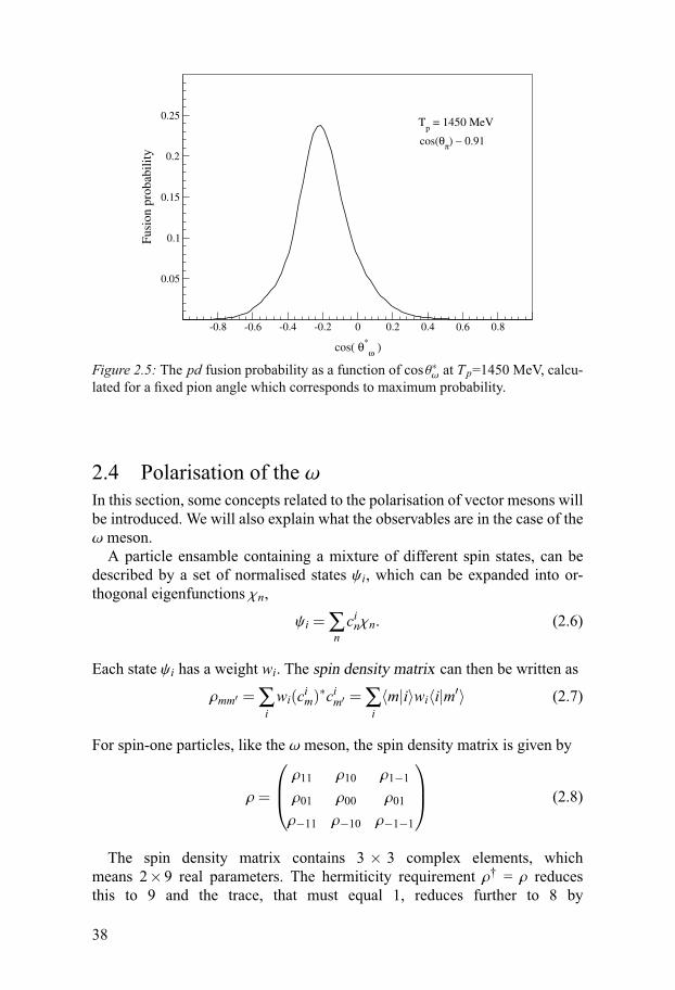
Figure 2.4: The pd fusion probability as a function of cosθ∗ω at Tp=1360 MeV, calcu-lated for a fixed pion angle which corresponds to maximum probability.

at equal excess energies [101]. Significant deviations from this could be a signof a strangeness component in the nucleon.

Violations of the OZI rule have been observed in many vector mesonproduction channels. For example, the DISTO collaboration found thatin pp→ ppX, the OZI rule is violated by an order of magnitude [102].SPESIII data on pp→ ppω [104] give, when compared to DISTO dataon pp→ ppφ [102] a similar result. Recent COSY data [103] found anenhancement with a factor 8 of the ω/φ ratio. In π−p→ nX data from Binnieet al. [59] it turned out that the OZI rule was violated by almost an order ofmagnitude. Backward scattering pd→ 3HeX data from SPESIV [70] show aviolation with a factor 20.

However, in many reactions, especially near the kinematic threshold innucleon-nucleon collisions, the dynamics of the nucleon-meson system aswell as the nucleon-nucleon system becomes important and it is very wellpossible that one or many resonances play a role in the production mecha-nism. Since the possible resonances participating in ω and φ production aredifferent, the production mechanisms of the two mesons can be quite differentand then the OZI rule may not be applicable. One should therefore study notonly the total cross sections but also observables more sensitive to the produc-tion mechanism, for example the angular distribution of the produced mesonand the angular distribution of its decay products. From the latter, the polar-isation of the vector meson can be extracted, which will be discussed in thefollowing section.

37

-0.8 -0.6 -0.4 -0.2 0 0.2 0.4 0.6 0.8

cos( θ∗ω )

0.05

0.1

0.15

0.2

0.25

Fusi

on p

roba

bilit

y

Tp = 1450 MeV

cos(θπ) ∼ 0.91

Figure 2.5: The pd fusion probability as a function of cosθ∗ω at Tp=1450 MeV, calcu-lated for a fixed pion angle which corresponds to maximum probability.

2.4 Polarisation of the ωIn this section, some concepts related to the polarisation of vector mesons willbe introduced. We will also explain what the observables are in the case of theω meson.

A particle ensamble containing a mixture of different spin states, can bedescribed by a set of normalised states ψi, which can be expanded into or-thogonal eigenfunctions χn,

ψi = ∑ncinχn. (2.6)

Each state ψi has a weight wi. The spin density matrix can then be written as

ρmm′ = ∑iwi(cim)∗cim′ = ∑

i〈m|i〉wi〈i|m′〉 (2.7)

For spin-one particles, like the ω meson, the spin density matrix is given by

ρ=

⎛⎜⎝ρ11 ρ10 ρ1−1

ρ01 ρ00 ρ01

ρ−11 ρ−10 ρ−1−1

⎞⎟⎠ (2.8)

The spin density matrix contains 3 × 3 complex elements, whichmeans 2×9 real parameters. The hermiticity requirement ρ† = ρ reducesthis to 9 and the trace, that must equal 1, reduces further to 8 by

38

Trρ = 1 = ρ11 + ρ−1−1 + ρ00. Three observables corresponds to the vectorpolarisation and five to the tensor polarisation. What will be measured in thiswork is one component of the tensor polarisation.

Symmetry reasons require ρ11 = ρ−1−1. Together with Trρ = 1 this leads to

ρ11 =12(1−ρ00). (2.9)

The angular distribution of the decay of a spin 1 meson as derived by K.Schilling et al. in [105]

W(cosθn,φn)=3

4π(ρ11 sin2 θ+ρ00 cos2 θ−

√2ρ10 sin2θcosφ−ρ1−1 sin2 θcos2φ),

(2.10)is dependent on the azimuthal angle φ. However, in a measurement with an un-polarised beam and an unpolarised target there is no φ-dependence. Equation2.10 is therefore integrated over φ giving

W(cosθ) ∝ ρ11 sin2 θ+ρ00 cos2 θ. (2.11)

Using 2.9 one obtains

W(cosθ) ∝ (1−ρ00)+(3ρ00−1)cos2 θ (2.12)

For the ω→ π+π−π0 decay it is convenient to describe the ω polarisation interms of the normal vector �n to the decay plane [106]. The normal is calculatedby the cross product of the momenta of two of the pions in the rest system ofthe ω meson. The angle θ in eq. 2.12 is the angle between the normal andsome quantisation axis.

Some information about the polarisation can be obtained by measuring oneof the three pions. The direction of the second, unobserved pion is averagedout [106] and the distribution of the angle θ1 between the direction of one pionand some reference axis then follows

W(cosθ1) ∝ (ρ00 +ρ±1±1)sin2 θ1 +2ρ±1±1 cos2 θ1 (2.13)

which, after using 2.9 simplifies to

W(cosθ1) ∝ (1+ρ00)− (3ρ00−1)cos2 θ1 (2.14)

The polarisation can also be studied in the other decay channel, i.e. ω→ π0γ.The information is then retrieved from the angular distribution of either the π0

or the γ, which should have the identical shape as the distribution describedin eq. 2.14 [106].

In a recent paper from MOMO [107], the polarisation of the φ meson inpd→ 3Heφ was measured by studying the angular distribution of the kaonsfrom the φ→ K+K− decay. It was found that the φ is produced almost com-

39

pletely polarised in the magnetic sub-state m = 0 along the beam direction. Ifthe ω is produced with different polarisation it would mean that the reactionmechanisms of the two mesons are different and that the strong violation ofthe OZI rule reported in [70] might be due to the nature of the meson-nucleoninteraction rather than details of the quark mixing.

2.5 Questions for this thesisFrom the previous discussions, ω production in the pd→3 Heω reaction isleft with several questions to be answered:• SPESIV observed a suppression in the production amplitude near threshold

[64], but the interpretation of the data has been critically discussed in [65,66]. By taking pd→3 Heω data at two beam energies, 1360 MeV and 1450MeV, i.e. one within and one above the energy region where the thresholdsuppression was observed, the validity of the SPESIV data can be tested.

• Only few data exist on the angular distribution of the ω from pd→3 Heω.Until recently, no attempts have been made to calculate the full angular dis-tribution theoretically. Two-step model calculations by K.P. Khemchandanisuggest that several partial waves in the πN→ Nω subprocess are relevantat both energies. Furthermore, poor velocity matching between the protonand the deuteron in the fusion into 3He is expected to suppress the differen-tial cross section at small and large angles. The only existing measurementof the angular distribution shows sharp rises, rather than suppressions, atthe extreme angles. The WASA detector covers the full angular range atboth 1360 MeV and 1450 MeV and can provide a significant advance ofthe existing data bank.

• The total cross section of pd →3 Heω has not been measured close tothreshold before. What are the cross sections at 1360 MeV and 1450 MeV?

• Is the OZI rule applicable in low energy nucleon-nucleon interactions?New data from the MOMO collaboration [107] show that the φ meson isproduced almost completely polarised in the pd→3 Heφ reaction. A differ-ent result for the ω meson would point towards different production mech-anisms of the two mesons. Large deviations from the OZI rule reported byseveral experiments could then originate from meson-nucleon interactionsrather than differences in the quark structure.

40

3. The CELSIUS/WASA experiment

3.1 The CELSIUS storage ringThe experiments in this work have been carried out at the The Svedberg Labo-ratory (TSL) in Uppsala, Sweden. The TSL provides accelerators for researchin physics, material science, biology and medicine.

The protons used for the measurements were first accelerated in the GustavWerner Cyclotron until they reached a kinetic energy of 185 MeV. The protonswere then injected into the CELSIUS 1 storage ring where they were furtheraccelerated [108]. The maximum kinetic energy for protons in the CELSIUSring was 1450 MeV, with electron cooling up to 550 MeV.

The CELSIUS ring operated until June 2005. It had a circumference of 82metres and consisted of four straight sections. The beam was injected in thefirst section and the WASA detector was installed in the second. The electron-cooling system was in the third section and in the fourth the CHICSi detectorwas installed, in figure 3.1 referred to as the Cluster Jet Target.2 In the fourbending sections, the beam was bent in arcs of 90o, each arc consisted of tendipole magnets sharing a common coil.

The CELSIUS operated in cycles of 180 seconds. First, the protons wereinjected, then the beam was accelerated to the desired kinetic energy (in ourcase up to 1360 MeV or 1450 MeV). This process took approximately 50 sec-onds. The magnetic field was then kept stable and the particles stored duringthe flat top, typically lasting from t1 = 55 s until t2 = 145 s. At the end of thecycle, the magnetic field was switched off and the beam was dumped. Before anew cycle could start, the magnets needed to return to the lower field strengthused during injection, which took roughly 30 seconds. The duty factor of thebeam was 50%.

3.2 The pellet targetThe idea of using a stream of discrete micro-spheres of hydrogen or deu-terium as an internal target was first suggested by Sven Kullander in 1984. The

1CELSIUS stands for Cooling with ELectrons and Storing of Ions from the Uppsala Syn-chrotron2further information about CHICSi can be found for example in [109]

41

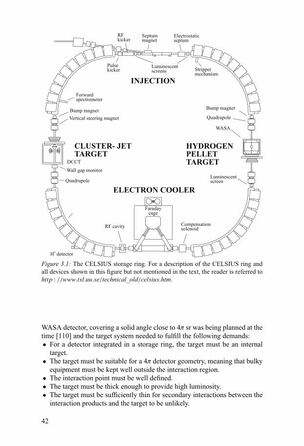
Figure 3.1: The CELSIUS storage ring. For a description of the CELSIUS ring andall devices shown in this figure but not mentioned in the text, the reader is referred tohttp : //www.tsl.uu.se/technical_old/celsius.htm.

WASA detector, covering a solid angle close to 4π sr was being planned at thetime [110] and the target system needed to fulfill the following demands:• For a detector integrated in a storage ring, the target must be an internal

target.• The target must be suitable for a 4π detector geometry, meaning that bulky

equipment must be kept well outside the interaction region.• The interaction point must be well defined.• The target must be thick enough to provide high luminosity.• The target must be sufficiently thin for secondary interactions between the

interaction products and the target to be unlikely.

42

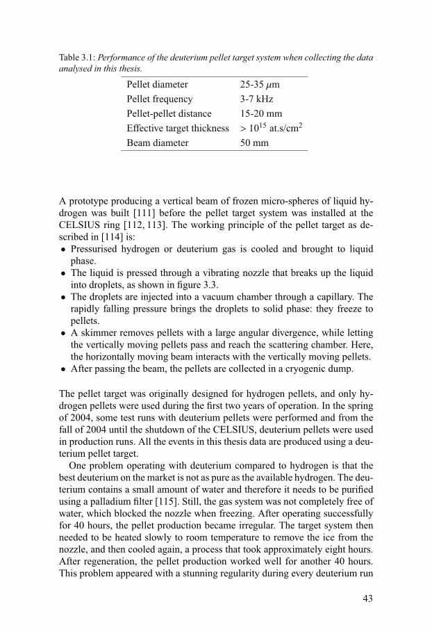
Table 3.1: Performance of the deuterium pellet target system when collecting the dataanalysed in this thesis.

Pellet diameter 25-35 μmPellet frequency 3-7 kHzPellet-pellet distance 15-20 mmEffective target thickness > 1015 at.s/cm2

Beam diameter 50 mm

A prototype producing a vertical beam of frozen micro-spheres of liquid hy-drogen was built [111] before the pellet target system was installed at theCELSIUS ring [112, 113]. The working principle of the pellet target as de-scribed in [114] is:• Pressurised hydrogen or deuterium gas is cooled and brought to liquid

phase.• The liquid is pressed through a vibrating nozzle that breaks up the liquid

into droplets, as shown in figure 3.3.• The droplets are injected into a vacuum chamber through a capillary. The

rapidly falling pressure brings the droplets to solid phase: they freeze topellets.

• A skimmer removes pellets with a large angular divergence, while lettingthe vertically moving pellets pass and reach the scattering chamber. Here,the horizontally moving beam interacts with the vertically moving pellets.

• After passing the beam, the pellets are collected in a cryogenic dump.

The pellet target was originally designed for hydrogen pellets, and only hy-drogen pellets were used during the first two years of operation. In the springof 2004, some test runs with deuterium pellets were performed and from thefall of 2004 until the shutdown of the CELSIUS, deuterium pellets were usedin production runs. All the events in this thesis data are produced using a deu-terium pellet target.

One problem operating with deuterium compared to hydrogen is that thebest deuterium on the market is not as pure as the available hydrogen. The deu-terium contains a small amount of water and therefore it needs to be purifiedusing a palladium filter [115]. Still, the gas system was not completely free ofwater, which blocked the nozzle when freezing. After operating successfullyfor 40 hours, the pellet production became irregular. The target system thenneeded to be heated slowly to room temperature to remove the ice from thenozzle, and then cooled again, a process that took approximately eight hours.After regeneration, the pellet production worked well for another 40 hours.This problem appeared with a stunning regularity during every deuterium run

43

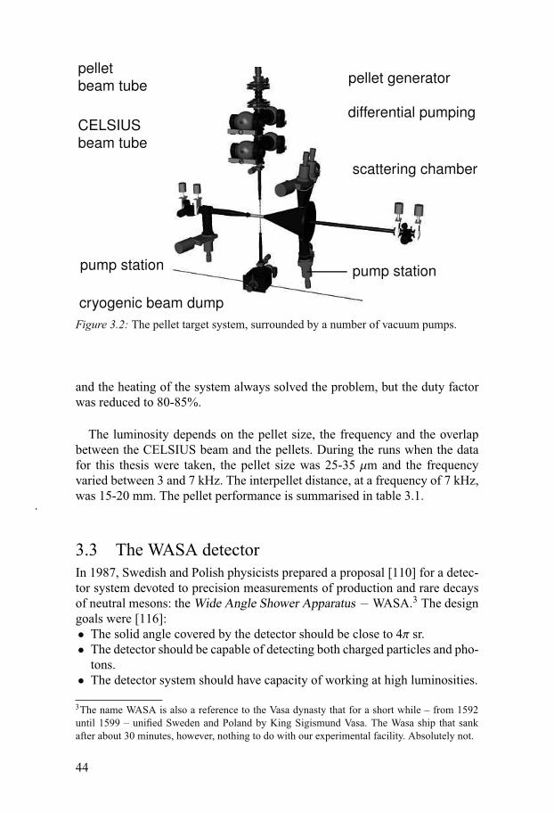
Figure 3.2: The pellet target system, surrounded by a number of vacuum pumps.

and the heating of the system always solved the problem, but the duty factorwas reduced to 80-85%.

The luminosity depends on the pellet size, the frequency and the overlapbetween the CELSIUS beam and the pellets. During the runs when the datafor this thesis were taken, the pellet size was 25-35 μm and the frequencyvaried between 3 and 7 kHz. The interpellet distance, at a frequency of 7 kHz,was 15-20 mm. The pellet performance is summarised in table 3.1.

3.3 The WASA detectorIn 1987, Swedish and Polish physicists prepared a proposal [110] for a detec-tor system devoted to precision measurements of production and rare decaysof neutral mesons: the Wide Angle Shower Apparatus −WASA.3 The designgoals were [116]:• The solid angle covered by the detector should be close to 4π sr.• The detector should be capable of detecting both charged particles and pho-

tons.• The detector system should have capacity of working at high luminosities.

3The name WASA is also a reference to the Vasa dynasty that for a short while – from 1592until 1599 – unified Sweden and Poland by King Sigismund Vasa. The Wasa ship that sankafter about 30 minutes, however, nothing to do with our experimental facility. Absolutely not.

44

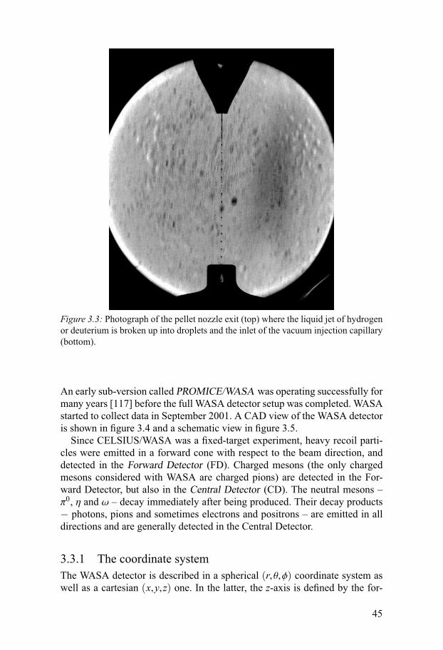
Figure 3.3: Photograph of the pellet nozzle exit (top) where the liquid jet of hydrogenor deuterium is broken up into droplets and the inlet of the vacuum injection capillary(bottom).

An early sub-version called PROMICE/WASA was operating successfully formany years [117] before the full WASA detector setup was completed. WASAstarted to collect data in September 2001. A CAD view of the WASA detectoris shown in figure 3.4 and a schematic view in figure 3.5.

Since CELSIUS/WASA was a fixed-target experiment, heavy recoil parti-cles were emitted in a forward cone with respect to the beam direction, anddetected in the Forward Detector (FD). Charged mesons (the only chargedmesons considered with WASA are charged pions) are detected in the For-ward Detector, but also in the Central Detector (CD). The neutral mesons –π0, η and ω – decay immediately after being produced. Their decay products− photons, pions and sometimes electrons and positrons – are emitted in alldirections and are generally detected in the Central Detector.

3.3.1 The coordinate systemThe WASA detector is described in a spherical (r, θ,φ) coordinate system aswell as a cartesian (x,y,z) one. In the latter, the z-axis is defined by the for-

45

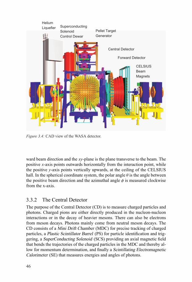
Pellet TargetGenerator

CELSIUSBeamMagnets

Central Detector

Forward Detector

HeliumLiquefier Superconducting

SolenoidControl Dewar

Figure 3.4: CAD view of the WASA detector.

ward beam direction and the xy-plane is the plane transverse to the beam. Thepositive x-axis points outwards horizontally from the interaction point, whilethe positive y-axis points vertically upwards, at the ceiling of the CELSIUShall. In the spherical coordinate system, the polar angle θ is the angle betweenthe positive beam direction and the azimuthal angle φ is measured clockwisefrom the x-axis.

3.3.2 The Central DetectorThe purpose of the Central Detector (CD) is to measure charged particles andphotons. Charged pions are either directly produced in the nucleon-nucleoninteractions or in the decay of heavier mesons. There can also be electronsfrom meson decays. Photons mainly come from neutral meson decays. TheCD consists of a Mini Drift Chamber (MDC) for precise tracking of chargedparticles, a Plastic Scintillator Barrel (PS) for particle identification and trig-gering, a SuperConducting Solenoid (SCS) providing an axial magnetic fieldthat bends the trajectories of the charged particles in the MDC and thereby al-low for momentum determination, and finally a Scintillating ElectromagneticCalorimeter (SE) that measures energies and angles of photons.

46

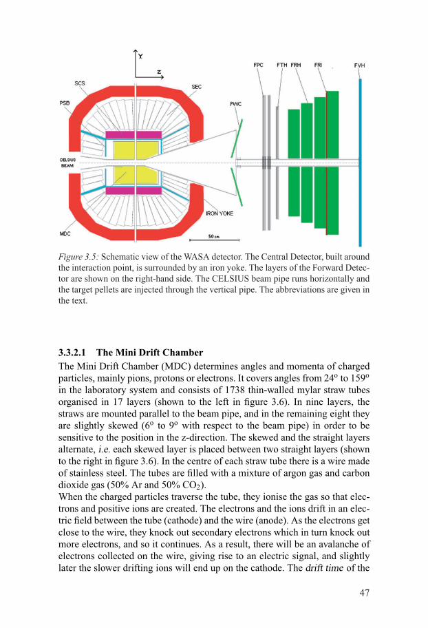
Figure 3.5: Schematic view of the WASA detector. The Central Detector, built aroundthe interaction point, is surrounded by an iron yoke. The layers of the Forward Detec-tor are shown on the right-hand side. The CELSIUS beam pipe runs horizontally andthe target pellets are injected through the vertical pipe. The abbreviations are given inthe text.

3.3.2.1 The Mini Drift ChamberThe Mini Drift Chamber (MDC) determines angles and momenta of chargedparticles, mainly pions, protons or electrons. It covers angles from 24o to 159o

in the laboratory system and consists of 1738 thin-walled mylar straw tubesorganised in 17 layers (shown to the left in figure 3.6). In nine layers, thestraws are mounted parallel to the beam pipe, and in the remaining eight theyare slightly skewed (6o to 9o with respect to the beam pipe) in order to besensitive to the position in the z-direction. The skewed and the straight layersalternate, i.e. each skewed layer is placed between two straight layers (shownto the right in figure 3.6). In the centre of each straw tube there is a wire madeof stainless steel. The tubes are filled with a mixture of argon gas and carbondioxide gas (50% Ar and 50% CO2).When the charged particles traverse the tube, they ionise the gas so that elec-trons and positive ions are created. The electrons and the ions drift in an elec-tric field between the tube (cathode) and the wire (anode). As the electrons getclose to the wire, they knock out secondary electrons which in turn knock outmore electrons, and so it continues. As a result, there will be an avalanche ofelectrons collected on the wire, giving rise to an electric signal, and slightlylater the slower drifting ions will end up on the cathode. The drift time of the

47

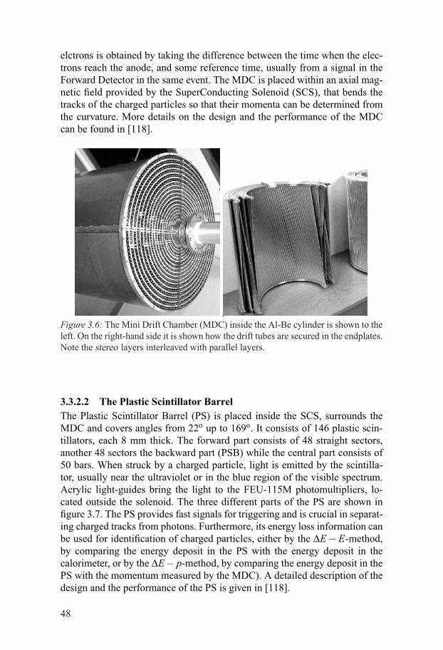
elctrons is obtained by taking the difference between the time when the elec-trons reach the anode, and some reference time, usually from a signal in theForward Detector in the same event. The MDC is placed within an axial mag-netic field provided by the SuperConducting Solenoid (SCS), that bends thetracks of the charged particles so that their momenta can be determined fromthe curvature. More details on the design and the performance of the MDCcan be found in [118].

Figure 3.6: The Mini Drift Chamber (MDC) inside the Al-Be cylinder is shown to theleft. On the right-hand side it is shown how the drift tubes are secured in the endplates.Note the stereo layers interleaved with parallel layers.

3.3.2.2 The Plastic Scintillator BarrelThe Plastic Scintillator Barrel (PS) is placed inside the SCS, surrounds theMDC and covers angles from 22o up to 169o. It consists of 146 plastic scin-tillators, each 8 mm thick. The forward part consists of 48 straight sectors,another 48 sectors the backward part (PSB) while the central part consists of50 bars. When struck by a charged particle, light is emitted by the scintilla-tor, usually near the ultraviolet or in the blue region of the visible spectrum.Acrylic light-guides bring the light to the FEU-115M photomultipliers, lo-cated outside the solenoid. The three different parts of the PS are shown infigure 3.7. The PS provides fast signals for triggering and is crucial in separat-ing charged tracks from photons. Furthermore, its energy loss information canbe used for identification of charged particles, either by the ΔE−E-method,by comparing the energy deposit in the PS with the energy deposit in thecalorimeter, or by the ΔE− p-method, by comparing the energy deposit in thePS with the momentum measured by the MDC). A detailed description of thedesign and the performance of the PS is given in [118].

48

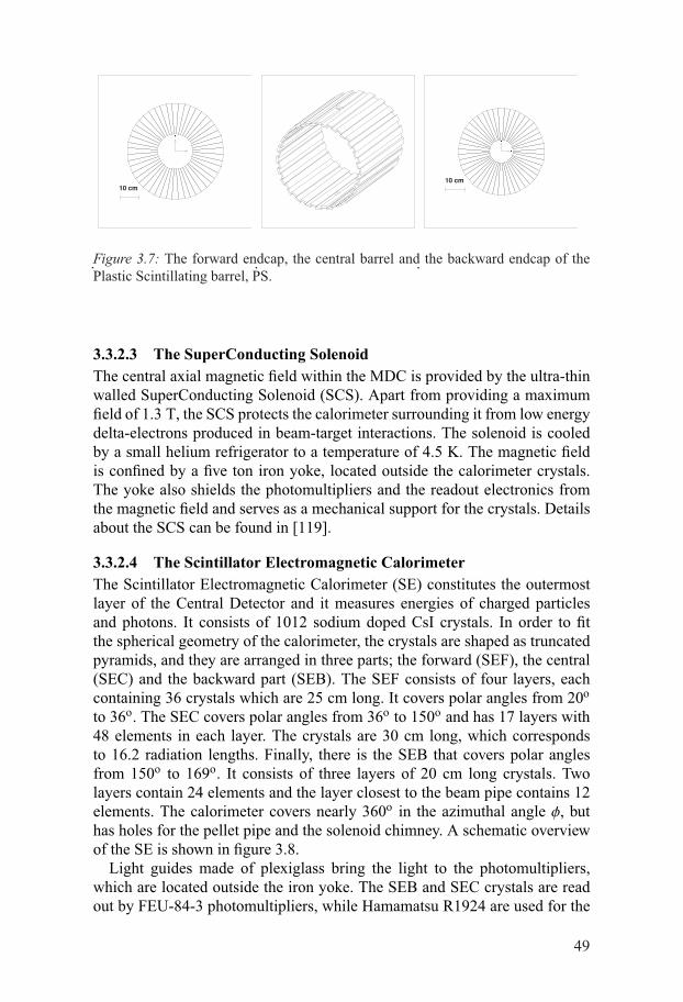
Figure 3.7: The forward endcap, the central barrel and the backward endcap of thePlastic Scintillating barrel, PS.

3.3.2.3 The SuperConducting SolenoidThe central axial magnetic field within the MDC is provided by the ultra-thinwalled SuperConducting Solenoid (SCS). Apart from providing a maximumfield of 1.3 T, the SCS protects the calorimeter surrounding it from low energydelta-electrons produced in beam-target interactions. The solenoid is cooledby a small helium refrigerator to a temperature of 4.5 K. The magnetic fieldis confined by a five ton iron yoke, located outside the calorimeter crystals.The yoke also shields the photomultipliers and the readout electronics fromthe magnetic field and serves as a mechanical support for the crystals. Detailsabout the SCS can be found in [119].

3.3.2.4 The Scintillator Electromagnetic CalorimeterThe Scintillator Electromagnetic Calorimeter (SE) constitutes the outermostlayer of the Central Detector and it measures energies of charged particlesand photons. It consists of 1012 sodium doped CsI crystals. In order to fitthe spherical geometry of the calorimeter, the crystals are shaped as truncatedpyramids, and they are arranged in three parts; the forward (SEF), the central(SEC) and the backward part (SEB). The SEF consists of four layers, eachcontaining 36 crystals which are 25 cm long. It covers polar angles from 20o

to 36o. The SEC covers polar angles from 36o to 150o and has 17 layers with48 elements in each layer. The crystals are 30 cm long, which correspondsto 16.2 radiation lengths. Finally, there is the SEB that covers polar anglesfrom 150o to 169o. It consists of three layers of 20 cm long crystals. Twolayers contain 24 elements and the layer closest to the beam pipe contains 12elements. The calorimeter covers nearly 360o in the azimuthal angle φ, buthas holes for the pellet pipe and the solenoid chimney. A schematic overviewof the SE is shown in figure 3.8.

Light guides made of plexiglass bring the light to the photomultipliers,which are located outside the iron yoke. The SEB and SEC crystals are readout by FEU-84-3 photomultipliers, while Hamamatsu R1924 are used for the

49

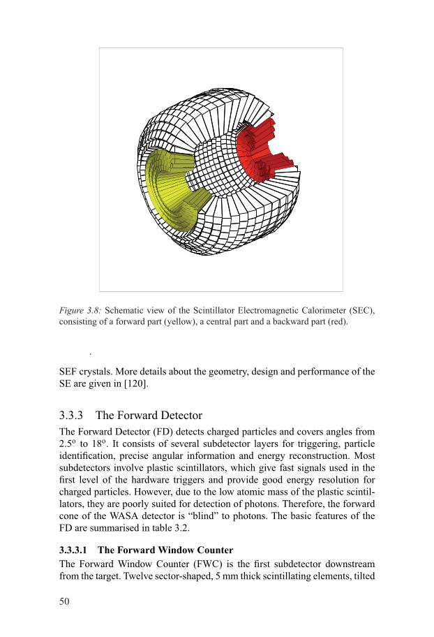
Figure 3.8: Schematic view of the Scintillator Electromagnetic Calorimeter (SEC),consisting of a forward part (yellow), a central part and a backward part (red).

SEF crystals. More details about the geometry, design and performance of theSE are given in [120].

3.3.3 The Forward DetectorThe Forward Detector (FD) detects charged particles and covers angles from2.5o to 18o. It consists of several subdetector layers for triggering, particleidentification, precise angular information and energy reconstruction. Mostsubdetectors involve plastic scintillators, which give fast signals used in thefirst level of the hardware triggers and provide good energy resolution forcharged particles. However, due to the low atomic mass of the plastic scintil-lators, they are poorly suited for detection of photons. Therefore, the forwardcone of the WASA detector is “blind” to photons. The basic features of theFD are summarised in table 3.2.

3.3.3.1 The Forward Window CounterThe Forward Window Counter (FWC) is the first subdetector downstreamfrom the target. Twelve sector-shaped, 5 mm thick scintillating elements, tilted

50

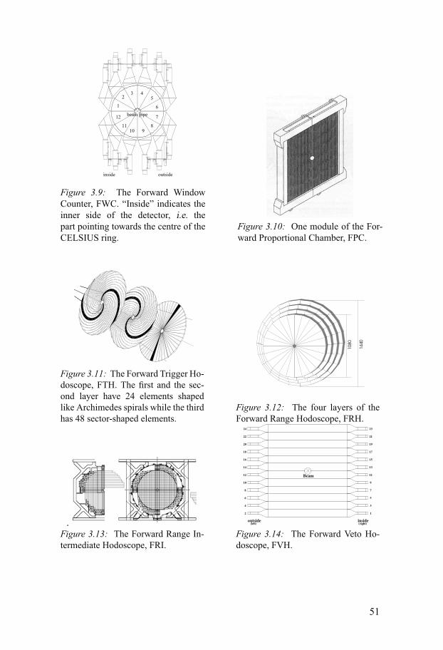
23 4

5

6

7

11

12

10 9

1

8

beam pipe

inside outside

Figure 3.9: The Forward WindowCounter, FWC. “Inside” indicates theinner side of the detector, i.e. thepart pointing towards the centre of theCELSIUS ring.

Figure 3.10: One module of the For-ward Proportional Chamber, FPC.

Figure 3.11: The Forward Trigger Ho-doscope, FTH. The first and the sec-ond layer have 24 elements shapedlike Archimedes spirals while the thirdhas 48 sector-shaped elements.

1440

1080

Figure 3.12: The four layers of theForward Range Hodoscope, FRH.

Figure 3.13: The Forward Range In-termediate Hodoscope, FRI.

Figure 3.14: The Forward Veto Ho-doscope, FVH.

51

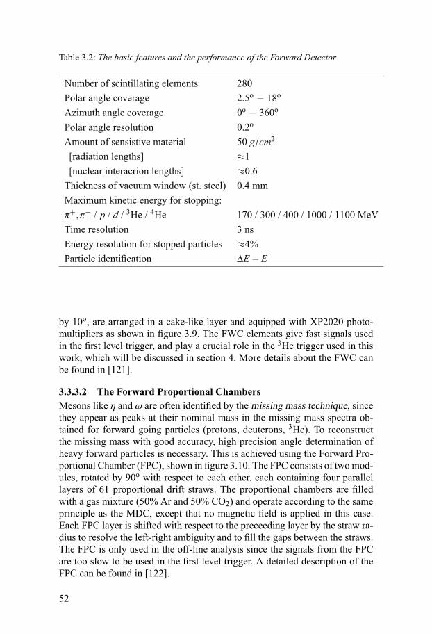
Table 3.2: The basic features and the performance of the Forward Detector

Number of scintillating elements 280Polar angle coverage 2.5o − 18o

Azimuth angle coverage 0o − 360o

Polar angle resolution 0.2o

Amount of sensistive material 50 g/cm2

[radiation lengths] ≈1[nuclear interacrion lengths] ≈0.6

Thickness of vacuum window (st. steel) 0.4 mmMaximum kinetic energy for stopping:π+,π− / p / d / 3He / 4He 170 / 300 / 400 / 1000 / 1100 MeVTime resolution 3 nsEnergy resolution for stopped particles ≈4%Particle identification ΔE−E

by 10o, are arranged in a cake-like layer and equipped with XP2020 photo-multipliers as shown in figure 3.9. The FWC elements give fast signals usedin the first level trigger, and play a crucial role in the 3He trigger used in thiswork, which will be discussed in section 4. More details about the FWC canbe found in [121].

3.3.3.2 The Forward Proportional ChambersMesons like η and ω are often identified by the missing mass technique, sincethey appear as peaks at their nominal mass in the missing mass spectra ob-tained for forward going particles (protons, deuterons, 3He). To reconstructthe missing mass with good accuracy, high precision angle determination ofheavy forward particles is necessary. This is achieved using the Forward Pro-portional Chamber (FPC), shown in figure 3.10. The FPC consists of two mod-ules, rotated by 90o with respect to each other, each containing four parallellayers of 61 proportional drift straws. The proportional chambers are filledwith a gas mixture (50% Ar and 50% CO2) and operate according to the sameprinciple as the MDC, except that no magnetic field is applied in this case.Each FPC layer is shifted with respect to the preceeding layer by the straw ra-dius to resolve the left-right ambiguity and to fill the gaps between the straws.The FPC is only used in the off-line analysis since the signals from the FPCare too slow to be used in the first level trigger. A detailed description of theFPC can be found in [122].

52

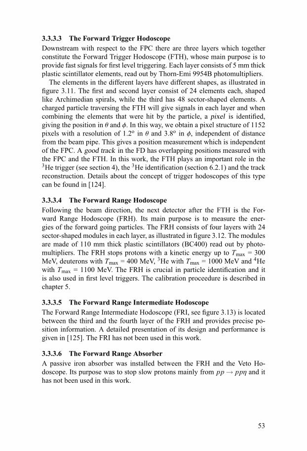
3.3.3.3 The Forward Trigger HodoscopeDownstream with respect to the FPC there are three layers which togetherconstitute the Forward Trigger Hodoscope (FTH), whose main purpose is toprovide fast signals for first level triggering. Each layer consists of 5 mm thickplastic scintillator elements, read out by Thorn-Emi 9954B photomultipliers.

The elements in the different layers have different shapes, as illustrated infigure 3.11. The first and second layer consist of 24 elements each, shapedlike Archimedian spirals, while the third has 48 sector-shaped elements. Acharged particle traversing the FTH will give signals in each layer and whencombining the elements that were hit by the particle, a pixel is identified,giving the position in θ and φ. In this way, we obtain a pixel structure of 1152pixels with a resolution of 1.2o in θ and 3.8o in φ, independent of distancefrom the beam pipe. This gives a position measurement which is independentof the FPC. A good track in the FD has overlapping positions measured withthe FPC and the FTH. In this work, the FTH plays an important role in the3He trigger (see section 4), the 3He identification (section 6.2.1) and the trackreconstruction. Details about the concept of trigger hodoscopes of this typecan be found in [124].

3.3.3.4 The Forward Range HodoscopeFollowing the beam direction, the next detector after the FTH is the For-ward Range Hodoscope (FRH). Its main purpose is to measure the ener-gies of the forward going particles. The FRH consists of four layers with 24sector-shaped modules in each layer, as illustrated in figure 3.12. The modulesare made of 110 mm thick plastic scintillators (BC400) read out by photo-multipliers. The FRH stops protons with a kinetic energy up to Tmax = 300MeV, deuterons with Tmax = 400 MeV, 3He with Tmax = 1000 MeV and 4Hewith Tmax = 1100 MeV. The FRH is crucial in particle identification and itis also used in first level triggers. The calibration proceedure is described inchapter 5.

3.3.3.5 The Forward Range Intermediate HodoscopeThe Forward Range Intermediate Hodoscope (FRI, see figure 3.13) is locatedbetween the third and the fourth layer of the FRH and provides precise po-sition information. A detailed presentation of its design and performance isgiven in [125]. The FRI has not been used in this work.

3.3.3.6 The Forward Range AbsorberA passive iron absorber was installed between the FRH and the Veto Ho-doscope. Its purpose was to stop slow protons mainly from pp→ ppη and ithas not been used in this work.

53

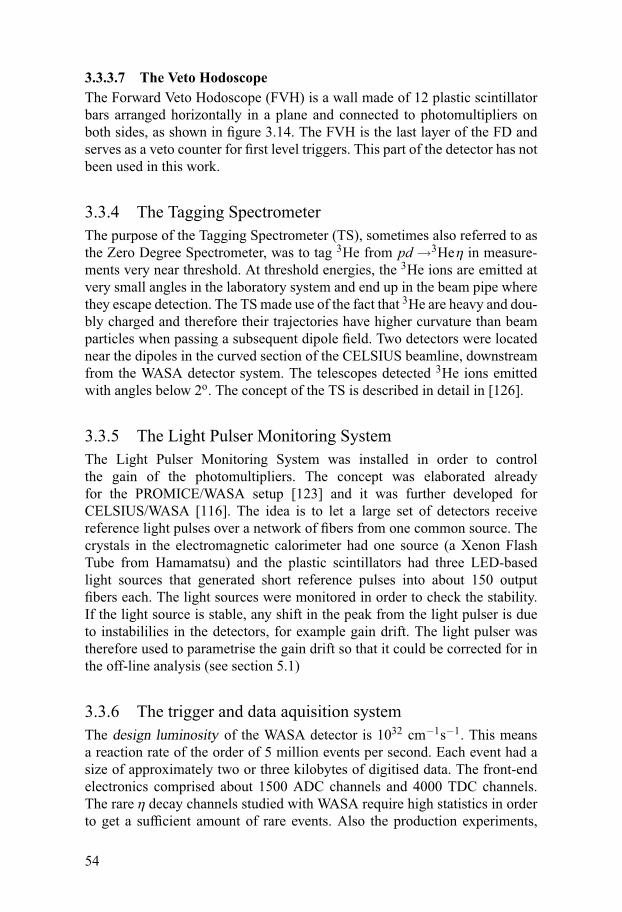
3.3.3.7 The Veto HodoscopeThe Forward Veto Hodoscope (FVH) is a wall made of 12 plastic scintillatorbars arranged horizontally in a plane and connected to photomultipliers onboth sides, as shown in figure 3.14. The FVH is the last layer of the FD andserves as a veto counter for first level triggers. This part of the detector has notbeen used in this work.

3.3.4 The Tagging SpectrometerThe purpose of the Tagging Spectrometer (TS), sometimes also referred to asthe Zero Degree Spectrometer, was to tag 3He from pd→3Heη in measure-ments very near threshold. At threshold energies, the 3He ions are emitted atvery small angles in the laboratory system and end up in the beam pipe wherethey escape detection. The TS made use of the fact that 3He are heavy and dou-bly charged and therefore their trajectories have higher curvature than beamparticles when passing a subsequent dipole field. Two detectors were locatednear the dipoles in the curved section of the CELSIUS beamline, downstreamfrom the WASA detector system. The telescopes detected 3He ions emittedwith angles below 2o. The concept of the TS is described in detail in [126].

3.3.5 The Light Pulser Monitoring SystemThe Light Pulser Monitoring System was installed in order to controlthe gain of the photomultipliers. The concept was elaborated alreadyfor the PROMICE/WASA setup [123] and it was further developed forCELSIUS/WASA [116]. The idea is to let a large set of detectors receivereference light pulses over a network of fibers from one common source. Thecrystals in the electromagnetic calorimeter had one source (a Xenon FlashTube from Hamamatsu) and the plastic scintillators had three LED-basedlight sources that generated short reference pulses into about 150 outputfibers each. The light sources were monitored in order to check the stability.If the light source is stable, any shift in the peak from the light pulser is dueto instabililies in the detectors, for example gain drift. The light pulser wastherefore used to parametrise the gain drift so that it could be corrected for inthe off-line analysis (see section 5.1)

3.3.6 The trigger and data aquisition systemThe design luminosity of the WASA detector is 1032 cm−1s−1. This meansa reaction rate of the order of 5 million events per second. Each event had asize of approximately two or three kilobytes of digitised data. The front-endelectronics comprised about 1500 ADC channels and 4000 TDC channels.The rare η decay channels studied with WASA require high statistics in orderto get a sufficient amount of rare events. Also the production experiments,

54

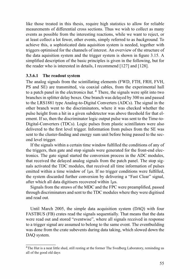
like those treated in this thesis, require high statistics to allow for reliablemeaurements of differential cross sections. Thus we wish to collect as manyevents as possible from the interesting reactions, while we want to reject, orat least collect a lot fewer, other events, simply referred to as background. Toachieve this, a sophisticated data aquisition system is needed, together withtriggers optimised for the channels of interest. An overview of the structure ofthe data aquisition system and the trigger system is shown in figure 3.15. Asimplified description of the basic principles is given in the following, but forthe reader who is interested in details, I recommend [127] and [128].

3.3.6.1 The readout systemThe analog signals from the scintillating elements (FWD, FTH, FRH, FVH,PS and SE) are transmitted, via coaxial cables, from the experimental hallto a patch panel in the electronics hut. 4 There, the signals were split into twobranches in splitter delay boxes. One branch was delayed by 300 ns and passedto the LRS1881 type Analog-to-Digital Converters (ADCs). The signal in theother branch went to the discriminators, where it was checked whether thepulse height from a hit in a given subdetector was above threshold for that el-ement. If so, then the discriminator logic output pulse was sent to the Time-to-Digital-Converters (TDCs). Logic pulses from plastic scintillators were alsodelivered to the first level trigger. Information from pulses from the SE wassent to the cluster-finding and energy sum unit before being passed to the sec-ond level trigger.

If the signals within a certain time window fulfilled the conditions of any ofthe triggers, then gate and stop signals were generated for the front-end elec-tronics. The gate signal started the conversion process in the ADC modules,that received the delayed analog signals from the patch panel. The stop sig-nals activated the TDC modules, that received all time information of pulsesemitted within a time window of 1μs. If no trigger conditions were fulfilled,the system discarded further conversion by delivering a “Fast Clear” signal,after which all data digitisers recovered within 1μs.

Signals from the straws of the MDC and the FPC were preamplified, passedthrough discriminators and sent to the TDC modules where they were digitisedand read out.

Until March 2005, the simple data acquisition system (DAQ) with fourFASTBUS (FB) crates read the signals sequentially. That means that the datawere read out and stored “eventwise”, where all signals received in responseto a trigger signal are assumed to belong to the same event. The eventbuildingwas done from the crate subevents during data taking, which slowed down theDAQ system.

4The Hut is a neat little shed, still resting at the former The Svedberg Laboratory, reminding usall of the good old days

55

From March 2005, a parallel readout system was implemented. Instead ofreading the data sequentially, the FB crates were read out in parallel. TheFB crates were controlled by one computer located in the electronics hut.The information from the crates was sent over parallel links and received bya dedicated PC, also located in the hut. The data were then sent over to acomputer in the counting room for on-line analysis and storing to the diskarrays.5 For the off-line analysis, the raw data had to be converted to eventformat by a special event-building software.

The former DAQ, with sequential readout of the FB crates, had a readouttime of ≈ 700μs/event, which corresponds to a readout rate of 1.4 kHz. Whenthe FB crates were read out in parallel, the readout time was 250-300 μs/event,which corresponds to a maximum readout rate of 3-4 kHz [129].

3.3.6.2 The trigger systemThere were two trigger levels, both implemented in hardware. They had shortprocessing times:≈200 ns for the first level and≈500 ns for the second level.

The first level trigger used signals from the fast plastic scintillators to checkmultiplicities, coincidences and hit alignment conditions to make a triggerdecision.

The simplest first level trigger was the frha1, that simply required at leastone hit in the FRH. It was considered as a minimum bias trigger since all reac-tions where a charged particle is emitted in the forward direction fire the frha1.This biases the total data sample very little since in a fixed-target experiment,there is almost always at least one forward going charged particle.

However, a simple trigger like the frha1 is dominated by the larger crosssection reactions and has a rate of a few hundred kHz. In addition, the frha1also collected a lot of background, for example particles emerging from inter-actions between for example beam halo and the beam pipe or beam and restgas.

To reduce the count rate of the minimum bias trigger, it had to be down-scaled, or prescaled, with a factor of 1000 to 5000. The trigger collecting mostof the data for this work aimed at enhancing the relative amount of events con-taining 3He. It was a first level trigger that required one hit with high energydeposit in the FWC aligned in the φ angle with a hit in the FTH or the FRH.6This will be described in detail in section 4.

The second level trigger used signals from the slower CsI crystals in the SEand information about cluster multiplicity and total energy deposit to take atrigger decision. The data collected for this thesis do not involve a second leveltrigger. The second level trigger is described in more detail in [120] and [127].

5more details about how the DAQ system works can be foundon http : //www.tsl.uu.se/̃ joze f /wasa4pi/DAQ/newdaq.html andhttp : //www.tsl.uu.se/̃ joze f /wasa4pi/DAQ/wasa_daq_v3.html.6Different detectors were used in different run periods

56

Trigger system

FASTBUS

ADC-LRS1881

TDC-LRS1876

Cratecontroller-1821

FASTBUS

ADC-LRS1881

TDC-LRS1876

Cratecontroller-1821

FASTBUS

TDC-LRS1876

Cratecontroller-1821

Patch panel

Discrim

LRS 4413

300 ns

300 ns

300 ns

300 ns

Discrim PM 96

300 ns Discrim

PM 98

Discrim PM 96 Preamp

Discrim Preamp

MUX PM 92

Front-endelectronics

PSB

FTH

FRH

FVH

FWC

SEC

MDC

FPC

1738

2000

96

96

64

24

1012 Cluster finding, Energy sum

First Level trigger

Second level trigger

Gate, Stop

Readoutsynchronization

Fast clear

1000

Disk storage

Midasserver

Gigabit link

Detectors

Event-buildingand

monitoring

FASTBUS

TDC-LRS1876

Cratecontroller-1821

Monitoring stations

RS-485 links4xPCI-7300A

DataAquisition

300 ns 146

300 ns 12

300 ns 4

FRI

ZD

Boards for trigger synch.and RS485 transmission

Figure 3.15: The front end electronics, trigger system and data aquisistion systemused in WASA. For a more detailed explanation of its different parts, the reader isreferred to [127].

57

4. The 3He trigger

All experimental data analysed in this thesis have been collected using a pro-ton beam impinging on a deuteron target. The reactions studied here all havea 3He in the final state.

Most reactions where a 3He is formed have much smaller cross sectionsthan reactions with p, n and d in the final state. For example, the pd→ 3Heωreaction should, according to the SPESIII measurement [67], have a total crosssection between 50 and 100 nb at Tp = 1450 MeV. Elastic pp-scattering at thesame energy has a cross section of≈24 mb [130], thus more than five orders ofmagnitude larger than the expected pd→ 3Heω cross section. An overwhelm-ing majority of the events collected by the minimum bias trigger, introducedin section 3.3.6.2, should originate from quasi-elastic pp- and pn-scatteringand quasi-free reactions such as pd→ ppπ0ns, pd→ ppπ+ns, pd→ dπ+nsand pd→ dπ0π+ns. 1 In order to get a reasonable amount of pd→ 3HeX data,a sophisticated trigger is needed, optimised to select 3He events.

4.1 High energy deposit in the FWCThe 3He nuclei passing through a given detector layer deposit more energyper unit length than protons and deuterons with the same velocity. A higherenergy deposit gives a higher light output in the scintillators which in turngives a higher amplitude of the generated signal. Requiring a high amplitudein a plastic scintillator detector should therefore suppress proton and deuteronevents. The FWC is used for this purpose: it provides fast signals, covers thefull angular range and as the first active material in the FD it is traversed byall forward going particles coming from the target, even the very slow ones.Furthermore, it has a modest position dependence. The position dependencecomes from the non-uniformity of the light collection efficiency; the amountof light collected by the photomultiplier depends on hit position. A study ofthe position dependence of the FWC was made using Tp = 400 MeV datafrom September 2003, produced by a proton beam impinging on a hydrogentarget. This data sample is very well-suited for performance studies, as shownin [131]. Figure 4.1 shows the polar angle θ in the laboratory system versusthe readout amplitude in one of the FWC elements. Although the readout am-plitude is slightly position (θ) dependent one can separate fast protons from

1The s in ns indicates that the neutron is a spectator in the reaction

59

deuterons from pp→ dπ+. Furthermore, 3He ions produced in pd collisionsgive a much larger amplitude than the protons and the deuterons seen in figure4.1.

Figure 4.1: The polar angle θ in the laboratory system versus the ADC readout am-plitude in one of the elements of the FWC for pp data at 400 MeV. The vertical bandcorresponds to fast protons from pp→ pp and the bump to deuterons from pp→ dπ+.The 3He ions produced in pd collisions give a much larger amplitude than the protonsand the deuterons seen in this picture.

The conclusion is that the FWC meets our requirements perfectly and it istherefore chosen to constitute the basis for the 3He trigger.

The energy deposit in the FWC was Monte Carlo simulated for a few reac-tions with different particles in the final state. The energy deposit of the 3Hewas found to be well separated from any other final state particle. This is il-lustrated in figure 4.2, where the light output from protons from quasi-elasticpp scattering and 3He ions from pd→ 3Heω are shown. However, the highenergy deposit tails of protons and deuterons overlap with the energy depositpeaks of the 3He. It should be noted that the areas under the curves in figure4.2 are not scaled to the cross sections of the two reactions. For example, thefive orders of magnitude higher cross section of elastic pp scattering com-pared to the pd→ 3Heω reaction, makes the high energy deposit tail of theelastic pp very important.

The first trigger test runs with a trigger purely based on high discriminatorthresholds in the FWC, named fwche3, were performed in March 2004. The

60

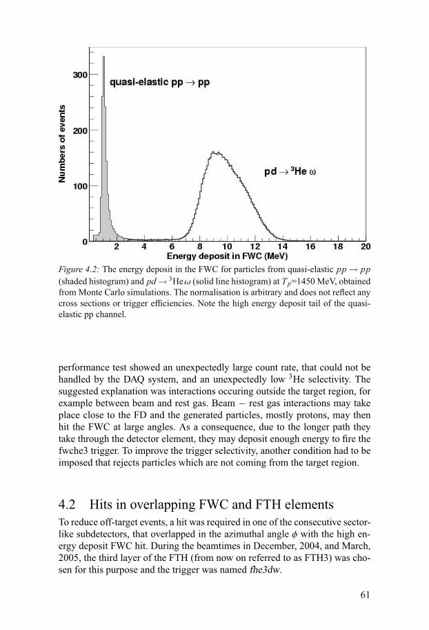
Figure 4.2: The energy deposit in the FWC for particles from quasi-elastic pp→ pp(shaded histogram) and pd→ 3Heω (solid line histogram) at Tp=1450 MeV, obtainedfrom Monte Carlo simulations. The normalisation is arbitrary and does not reflect anycross sections or trigger efficiencies. Note the high energy deposit tail of the quasi-elastic pp channel.

performance test showed an unexpectedly large count rate, that could not behandled by the DAQ system, and an unexpectedly low 3He selectivity. Thesuggested explanation was interactions occuring outside the target region, forexample between beam and rest gas. Beam − rest gas interactions may takeplace close to the FD and the generated particles, mostly protons, may thenhit the FWC at large angles. As a consequence, due to the longer path theytake through the detector element, they may deposit enough energy to fire thefwche3 trigger. To improve the trigger selectivity, another condition had to beimposed that rejects particles which are not coming from the target region.

4.2 Hits in overlapping FWC and FTH elementsTo reduce off-target events, a hit was required in one of the consecutive sector-like subdetectors, that overlapped in the azimuthal angle φ with the high en-ergy deposit FWC hit. During the beamtimes in December, 2004, and March,2005, the third layer of the FTH (from now on referred to as FTH3) was cho-sen for this purpose and the trigger was named fhe3dw.

61

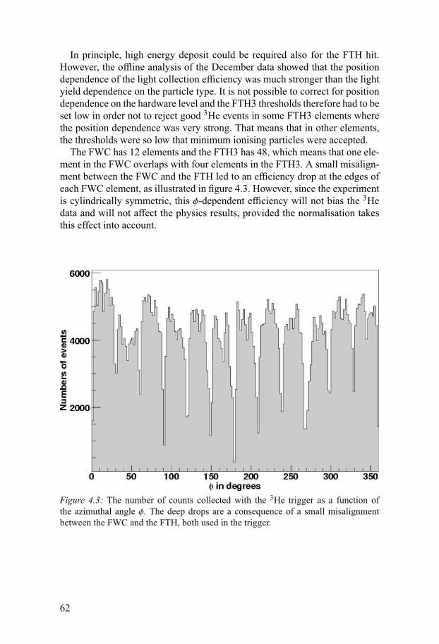
In principle, high energy deposit could be required also for the FTH hit.However, the offline analysis of the December data showed that the positiondependence of the light collection efficiency was much stronger than the lightyield dependence on the particle type. It is not possible to correct for positiondependence on the hardware level and the FTH3 thresholds therefore had to beset low in order not to reject good 3He events in some FTH3 elements wherethe position dependence was very strong. That means that in other elements,the thresholds were so low that minimum ionising particles were accepted.

The FWC has 12 elements and the FTH3 has 48, which means that one ele-ment in the FWC overlaps with four elements in the FTH3. A small misalign-ment between the FWC and the FTH led to an efficiency drop at the edges ofeach FWC element, as illustrated in figure 4.3. However, since the experimentis cylindrically symmetric, this φ-dependent efficiency will not bias the 3Hedata and will not affect the physics results, provided the normalisation takesthis effect into account.

Figure 4.3: The number of counts collected with the 3He trigger as a function ofthe azimuthal angle φ. The deep drops are a consequence of a small misalignmentbetween the FWC and the FTH, both used in the trigger.

62

Table 4.1: The trigger conditions that have been used for 3He collection in this work(upper part) and the trigger conditions that were tested but not used in the productionmode of the experiment (lower part)

Trigger name Descriptionfrha1 at least one hit in the first layer of the FRHfwche3 high discriminator threshold in the FWCfhe3dw high discriminator threshold in the FWC

with a hit in an overlapping element in the FTH3fhe3rw high discriminator threshold in the FWC

with a hit in an overlapping element in the FRHfhd3he3 high discriminator threshold in the FTH3vfwc2 veto on more than one hit in the FWCvfhds2 veto on more than one hit in the FTH3vfvh1 no hit in the FVHvps no hit in the PSse2n two neutral clusters in the SE

(second level trigger)

4.3 Summary of trigger conditionsIn table 4.1, the different trigger conditions that have used for 3He tagging,are summarised:

4.4 The 3He trigger performanceFor the trigger performance, the following aspects are of special importance:• The rate of the trigger should not exceed the maximum data acquisition

rate that can be achieved.• The absolute 3He yield should be as high as possible.• The bias of the data sample selected by the trigger should ideally be neg-

ligble. If a bias cannot be avoided, it must be well understood and correctedfor.Measuring the trigger rate and the 3He yield is trivial, while the bias needs

some thought. Generally, the simpler trigger, the smaller the bias. With secondlevel triggers, which check cluster multiplicities in the CD or total energy de-posits, specific decay channel are preferred. This introduces a bias of the datawhose effects must be understood and corrected for. When triggers based onhigh discriminator thresholds are used, the effects of the thresholds need to be

63

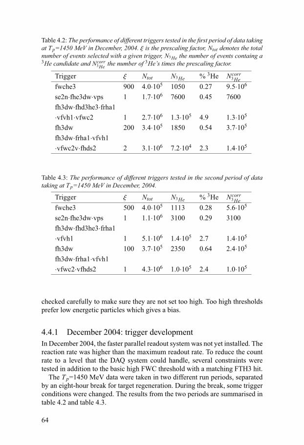
Table 4.2: The performance of different triggers tested in the first period of data takingat Tp=1450 MeV in December, 2004. ξ is the prescaling factor, Ntot denotes the totalnumber of events selected with a given trigger, N3He the number of events containg a3He candidate and Ncorr3He the number of

3He’s times the prescaling factor.

Trigger ξ Ntot N3He % 3He Ncorr3Hefwche3 900 4.0·105 1050 0.27 9.5·106

se2n·fhe3dw·vps 1 1.7·106 7600 0.45 7600fh3dw·fhd3he3·frha1·vfvh1·vfwc2 1 2.7·106 1.3·105 4.9 1.3·105

fh3dw 200 3.4·105 1850 0.54 3.7·105

fh3dw·frha1·vfvh1·vfwc2v·fhds2 2 3.1·106 7.2·104 2.3 1.4·105

Table 4.3: The performance of different triggers tested in the second period of datataking at Tp=1450 MeV in December, 2004.

Trigger ξ Ntot N3He % 3He Ncorr3Hefwche3 500 4.0·105 1113 0.28 5.6·105

se2n·fhe3dw·vps 1 1.1·106 3100 0.29 3100fh3dw·fhd3he3·frha1·vfvh1 1 5.1·106 1.4·105 2.7 1.4·105

fh3dw 100 3.7·105 2350 0.64 2.4·105

fh3dw·frha1·vfvh1·vfwc2·vfhds2 1 4.3·106 1.0·105 2.4 1.0·105

checked carefully to make sure they are not set too high. Too high thresholdsprefer low energetic particles which gives a bias.

4.4.1 December 2004: trigger developmentIn December 2004, the faster parallel readout system was not yet installed. Thereaction rate was higher than the maximum readout rate. To reduce the countrate to a level that the DAQ system could handle, several constraints weretested in addition to the basic high FWC threshold with a matching FTH3 hit.

The Tp=1450 MeV data were taken in two different run periods, separatedby an eight-hour break for target regeneration. During the break, some triggerconditions were changed. The results from the two periods are summarised intable 4.2 and table 4.3.

64

This is what was learned from the trigger testing in more detail:The veto triggers− vps, vfwc2, vfhds2 and vfvh1− reduced the count rate

effectively but also bias the data.The vfwc2 and vfhds2 rejected events with more than one forward goingparticle. For example, events from the pd→3HeX reaction with charged pi-ons moving forwards. Monte Carlo simulations show that vfwc2 and vfhds2should reduce the acceptance of the pd→ 3Heω,ω→ π+π−π0 with 20%.The vfvh1 has a similar effect, by rejecting all fast forward going particles. No3He produced at this energy had sufficient energy to reach the FVH, but manycharged pions were fast enough to punch through all detector layers, reach theveto hodoscope and fire the veto. The bias that these vetoes introduce is easilyunderstood and accounted for by Monte Carlo simulations.

Veto triggers also reject events that accidentally contain particles fromother, time-overlapping events. Furthermore, vetoes can be fired by a noisydetector element. To summarise, veto triggers may reject good eventsand the effects they introduce are difficult to simulate and account for.Therefore, the triggers containing vetoes, for example the se2n·fhe3dw·vpstrigger, were not used in March and May 2005 when the experiment wasoperating in the production mode. The se2n·fhe3dw·vps also rejected allevents with charged particles in the CD which makes it unsuitable for thepd→3 Heω, ω→ π+π−π0 reaction.

The high discriminator thresholds of the FTH3 applied in the fhd3he3 trig-ger, imposed an efficiency reduction due to the strong position dependence ofsome of the FTH3 elements. The strong position dependence was not knownbefore the December run but was discovered later in the off-line analysis ofthe data. The fhd3he3 biased the data sample by prefering events containinglow energy 3He. The fhd3he3 condition was therefore abandoned during thedata taking periods in March and May 2005.

The simple fhe3dw trigger had a low bias as expected but a high count rate.Therefore, to match the DAQ capacity, it had to be prescaled by a large factor.However, since the fhe3dw trigger was best understood, the triggers used inMarch 2005 and May 2005 were based on the fhe3dw condition.

4.4.2 March 2005:production runThe faster data acquisition system (see section 3.3.6.1) was implemented be-fore the March run, and enabled a trigger rate that was more than twice aslarge compared to the test runs in December 2004. It was therefore sufficientto use the simple fhe3dw condition in combination with the frha1, i.e. at leastone hit in the FRH, with no prescaling.

65

4.4.3 May 2005:production runFor the May run, the 3He trigger was further improved by replacing thefhe3dw·frha1 with the fhe3rw trigger. The fhe3rw was tested for a few hoursduring the March run and required one high energy deposit hit in the FWCand a matching hit in the first layer of the FRH. Since the FRH is furtherdownstream from the target than the FTH3, the hit overlap requirement hasmore efficient. The discriminator thresholds had to be low also in the FRHcase, but not due to any position dependence but due to the fact that 3He ionsin the FRH have a very large spread in the energy deposit. The fhe3rw triggerhad a low bias and could be used without prescaling.

66

5. Calibration

A careful detector calibration is crucial if a high data quality is to be achieved.Before details of the calibration are given, we will shortly describe what

happens when a particle traverses the material in a detector:The Forward Trigger Hodoscope and the Forward Range Hodoscope in theForward Detector are made of plastic scintillators. The electromagneticcalorimeter in the Central Detector consist of scintillating CsI crystals. Whena charged particle traverses a scintillator, it excites and ionises the atoms inthe material. When the atoms de-excites, photons (typically visible light)are emitted. The light is brought to a photomultiplier (PM-tube), where ithits a photocathode. When photons hit the photocathode, photoelectronsare released. The number of electrons is then multiplied in the PM-tubebefore they hit an anode, which creates an electric pulse. The height of thepulse is proportional to the number of photons entering the photomultiplier.This in turn is proportional to the energy deposited in the scintillator by theincoming particle. The light collection efficiency depends on the geometry ofthe detector. Also, the light yield for a given energy deposit, depends on theparticle type.

In addition, there may be unwanted, time dependent effects that must be un-derstood and corrected for. The gain of the amplifier and the high voltage be-tween the dynodes in the photomultiplier depends on experimental conditionssuch as temperature, the dynode voltage and the count rate. These parametersare neither stable during a period of data taking nor between different periodsof data taking.

5.1 Calibration of the Forward DetectorThis section treats the energy calibration of the plastic scintillator detectors inthe FD: the FWC, the FTH and the FRH.

5.1.1 Gain correction due to count rateThe count rate in the Forward Detector can vary quite dramatically in a shorttime, due to varying pellet rate. Especially by the end of every run period,the pellet rate jumps up and down very abruptly − sometimes on a time scaleof less than a second. A study on how this variation affected the gain of the

67

photomultipliers, showed that the gain may change with as much as 10% inone accelerator cycle, if the count rate is very unstable. These effects can beexplained by high rate of particles increasing the current flow in the photo-multipliers which can affect the voltages on the dynodes and thus the gain.

This effect was parametrised and corrected for in the following way: Dur-ing the last hours of data taking in March, 2005, the pellet rate was highlyunstable, causing the count rate to fluctuate between almost zero up to 500kHz several times per minute. Data from this run were therefore used for theparametrisation of the readout amplitude as a function of the count rate. Thisstudy was done using minimum ionising particles which give a well definedenergy deposit in the detector layer they traverse. The data were divided intobins depending on the count rate. For each count rate bin, the signal ampli-tude was histogrammed and the peak position calculated. For every detectorelement in the FTH and the FRH, the peak position versus the count rate wasplotted and parametrised by fitting a straight line to the data.

In the data analysis, the signal amplitude in a given element is then cor-rected for using this linear parametrisation and the recorded count rate.

5.1.2 Long term time dependent correctionsSince minimum ionising protons have a well defined energy deposit in thedetectors, they appear in a peak in energy deposit histograms. The position ofthis peak drifts slightly in time, on short time scales due to variations in thecount rate, but also on longer time scales due to drifting gain. This long termeffect has to be parametrised and corrected for in the analysis.

For this purpose, the light pulser was used. In the off-line analysis, his-tograms were filled automatically for every detector element with the readoutamplitude obtained with the light pulser trigger. When enough statistics wasreached, a correction factor was calculated by comparing the peak position toa reference peak.1 All amplitudes corresponding to a given detector are thenmultiplied by the correction factor obtained for this detector until the nextcorrection factor is found (typically every 70 seconds).

In addition to the PM instabilities, the scintillators themselves could alsohave a time dependent behaviour if their light yield is temperature dependent.The temperature in the CELSIUS hall varied between 15oC and 25oC duringthe run periods when the data for this work were taken. However, a recentstudy of the light yield from the plastic scintillators in the FRH showed thatthis effect is not significant [132].

1the average peak position obtained using all data from the run period being analysed

68

5.1.3 Geometrical correctionsAn important effect in scintillating detector elements is light collection effi-ciency. The elements in the FWC, FTH3 and the FRH are sector-shaped withPM-tubes mounted on the outer ends. If the particle hits the element at a smallpolar angle θ, the emitted photons are less likely to hit the photocathode com-pared to if the particle hits the element at a large angle close to the photocath-ode. Therefore, the light collection effiency increases with increasing polarangle.

This effect is parametrised using protons stopping one layer downstreamfrom the layer being studied. The proton sample is then divided into 15 binsfrom θp = 3o to θp = 18o and the readout amplitude is histogrammed in eachbin. The peak position is then parametrised as a third order polynomial in θand the light collection efficiency is corrected for in the analysis.

5.1.4 Light quenchingDifferent particles have different dependence between light yield anddeposited energy; heavily ionising particles produce less light per unit energythan those with small ionisation densities. This effect, sometimes referred toas the quenching effect, is a saturation effect that has been subject of manytheoretical and experimental investigations (see for example [133] and [134]).According to Ref. [133], the amount of fluorescent light emitted per unit pathlength x is given by the formula

dSdx

=AdEdx

1+ kBdEdx(5.1)

where dE/dx is the particle’s energy loss per unit path length, A is a constantthat depends on the type of material and kB is a constant that depends on theparticle type and the material.

In this work, the light yield curves from the Bicron BC-400 data sheet werefitted to equation 5.1 and the constants [133] kB were found for p, d and 4He.The kB constant for 3He was assumed to be the same as for 4He.

5.1.5 Summary: The calibration formulaHaving parametrised the important effects, the energy deposit ΔE in a givendetector layer can be calculated from the signal amplitude v. The gain driftdue to count rate and the long term gain drifts are first corrected for:

vcorr = v ·wLT · ( fCR+gCR · cr), (5.2)

where vcorr is the corrected amplitude, fCR and gCR are constants from thecount rate parametrisation, cr is the count rate and wLT the long term correc-

69

tion factor. From vcorr, the amount of light reaching the PM-tube LPM is givenby

LPM = bvcorrecvcorr , (5.3)

where b and c are calibration constants, obtained by comparing fitted his-tograms of stopping protons, deuteron and 3He from experimental data to fit-ted histograms obtained with Monte Carlo.

The geometrical paramtrisation of the light collection efficiency is then usedto calculate the amount of produced fluorescent light L(ΔE):

L(ΔE) = (1+a1 · r+a2 · r2 +a3 · r3)LPM (5.4)

where a1, a2 and a3 are constants from the parametrisation of the positiondependence of the light collection efficiency, and r the distance from the centreof the beam to the impact point.

Knowing L(ΔE), the particle can be identified, which will be explainedin section 6.2.1. When the particle ID is known, the energy deposit can becalculated using equation 5.1 in section 5.1.4.

5.2 Time calibration of the plastic scintillatorsIn order to build tracks from hits in the detectors, one has to know the timesat which the hits occured and compare them to a reference time at which theevent took place, t0. To make such a comparison possible, one has to calibratethe time signals in such a way that hits occuring at the same time give thesame time signal.

The reference time is obtained from the fast signals from the plastic scintil-lators in the FD (usually the FTH) but one can also use the PS. The referencetime is described by the expression

t0 = tTDC− tTOF− tscint− to f f (5.5)

where tTDC is the TDC readout, tTOF is the time of flight for the particleto reach an element in the FTH, tscint the time propagation of the light inthe plastic scintillator and to f f the time offset of the detector element. tTOFdepends on the mass, the energy and the distance travelled by the particle.to f f is specific for each element and is the summed effect of signal delayin the cables, photomultiplier response and electronics delay. Before startingthe physics analysis of a data set, the to f f of each element must be obtained.When analysing a different data set, from a different data taking period wherethe experimental conditions have been changed, new to f f constants must beobtained. The to f f is trigger dependent, and therefore, the routine that findsthe time offsets takes data collected with the 3He trigger only.

70

5.3 Calibration of the Central DetectorThe Scintillator Electromagnetic Calorimeter, the Mini Drift Chamber and thePlastic Scintillating Barrel have all been used when analysing the data for thisthesis. However, the PS was only used for particle identification by checkingwhether there was a signal or not and did therefore not need to be energy cal-ibrated (signal = charged particle, no signal = photon). To calibrate the MDC,the time offsets to f f for each straw in each run period have been determined.Then the relation between the drift time and drift distance is calculated foreach layer of the MDC. The basic algorithm is described in [118]

5.3.1 Calibration of the Electromagnetic CalorimeterIn this work, the Scintillator Electromagnetic Calorimeter has only beenused for measurement of photon energies, and the calibration is thereforeperformed using photons. The CsI crystals in the SE were calibrated atvarious times (see for example Ref. [120]) but since the high voltages in thePM-tubes and the properties of the crystals change over time, the calibrationconstant needs to be updated regularly. This is a complicated process formainly two reasons: first, there is no high cross section process where singlephotons with a known energy are produced. Therefore, photons from π0

decays are used. Second, the energy of one photon is deposited in severalneighbouring crystals due to the development of an electromagnetic shower.The calibration of the CsI crystals is carried out in the following way:• A combination of two photons having an invariant mass fairly close to theπ0 mass is identified (if any).

• For each π0 candidate, the crystal with the largest energy deposit is identi-fied.

• The histogram of the γγ invariant mass is then updated for each crystalwith the highest energy deposit.

• If the π0 peak position for a given crystal is shifted with respect to the π0

mass, it is assumed that it is due to a bad calibration constant of this detector(the contributions from the other participating crystals are averaged out)and the calibration constant is adjusted accordingly.

• The procedure is repeated until all crystals give peaks centered at the π0

mass.This method does, of course, only work if a rough calibration is already per-formed. Another drawback is that the calibration is optimised for photonscoming from π0 decays. The mass resolution for η→ γγ and ω → π0γ ismodest since the photons from these decay have higher energies.

71

6. Analysis

6.1 SoftwareIn the simulations, the event generation is performed by the phace spaceMonte Carlo programs FOWL [135] and GENBOD [136]. The WASAdetector description is implemented in a Monte Carlo program based on theGEANT3 [137] package from CERN and describes particle interactions withthe detector material. This includes energy losses through ionisation, pairproduction, nuclear interactions, Cherenkov radiation and other physicalprocesses whose effects are well known. The GEANT3 description of theWASA detector does not include electronic noise or other, less well-knowneffects such as the light collection efficiency of the scintillators. Instead, anadditional smearing factor is added for each detector part to compensate forthe unknown effects in the simulations.

The analysis of simulated as well as experimental data was performed us-ing the software package ODIN (Online/Offline Data INspection) developedby Jozef Zlomanczuk.1 ODIN has been built around the MULTI [138] soft-ware package developed at Fermilab in the 1970’s. For graphics and fitting ofhistograms, ROOT was used.2

6.2 Particle identification6.2.1 Identification in the Forward DetectorIn the Forward Detector, a preliminary particle ID is first obtained by the“ΔE− E”-method, i.e. by comparing the energy deposit in the layer wherethe particle stops, with the energy deposit in the preceding layer. Or more cor-rectly, it is the amount of collected fluorescent light, rather than the energydeposit that is compared; as was discussed in section 5.1.4, different parti-cles have different relations between energy and light in scintillators due tothe quenching effect. Hence, before calibration, it is the light output that ismeasured.

In a “ΔE− E”-plot, different particles will show up in different bands, asillustrated in figure 6.1, corresponding to particles stopping in the second layerof the FRH. The 3He ions appear in the uppermost band. Below is a band

1http : //www.tsl.uu.se/̃ joze f /wasa4pi/Odin/ODIN_Users_guide.pd f2http : //www.root.cern.ch/root

73

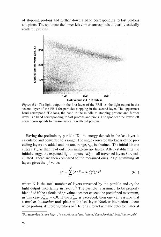
of stopping protons and further down a band corresponding to fast protonsand pions. The spot near the lower left corner corresponds to quasi-elasticallyscattered protons.

Figure 6.1: The light output in the first layer of the FRH vs. the light output in thesecond layer of the FRH for particles stopping in the second layer. The uppermostband correspond 3He ions, the band in the middle to stopping protons and furtherdown is a band corresponding to fast protons and pions. The spot near the lower leftcorner corresponds to quasi-elastically scattered protons.

Having the preliminary particle ID, the energy deposit in the last layer iscalculated and converted to a range. The angle corrected thickness of the pre-ceding layers are added and the total range, rtot, is obtained. The initial kineticenergy Tini is then read out from range-energy tables. After establishing theinitial energy, the expected light outputs, ΔLci , in all traversed layers i are cal-culated. These are then compared to the measured ones, ΔLmi . Summing alllayers gives the χ2 value:

χ2 =N

∑i=1

(ΔLmi −ΔLci )2)/σ2i (6.1)

where N is the total number of layers traversed by the particle and σi thelight output uncertainty in layer i.3 The particle is assumed to be properlyidentified if the calculated χ2 value does not exceed the predefined maximum,in this case χ2

max = 6.0. If the χ2max is exceeded, then one can assume that

a nuclear interaction took place in the last layer. Nuclear interactions occurwhen protons, deuterons, tritons or 3He ions interact with the detector material

3For more details, see http : //www.tsl.uu.se/̃ joze f /docs/ f iles/ParticleIdenti f ication.pd f

74

and either scatter elastically or induce nuclear reactions so that other particlesare produced. After a nuclear interaction, the energy deposit in the remainingdetector layers are very different from the those expected for a particle sloweddown via interactions with electrons.

The last layer is then omitted from the analysis and only the N− 1 layers,passed by the particle before the assumed interaction, are taken into account.Since the original ΔE−E relation makes no sense and the preliminary parti-cle ID may be wrong, one has to find out for which particle from the list ofexpected final state particles it is possible to get the best match between calcu-lated and measured ΔLci . If such a particle is found and gives a χ2 (accordingto 6.1) below χ2

max, then that particle is accepted as properly identified. If not,then the last layer is removed from the analysis and whole proceedure repeateduntil χ2 ≤ χ2

max or until no more FRH layers remain.

6.2.2 Identification in the Central DetectorA cluster in the SE with no matching hit in the PS is defined as a photon.If, on the other hand, a SE cluster or an MDC track has a matching PS hit,they come from a charged particle. To determine the mass of a charged par-ticle, the momentum and energy have to be determined. The momentum canbe measured from the curvature of the MDC track in the solenoid field. Theenergy can be measured in the SE, but in many cases, the particle does nothave sufficient energy to reach the calorimeter. Then, the energy deposit inthe PS can be used instead. A nice example of how this can be carried out, isgiven in [139]. In this work however, only photons are identified properly inthe Central Detector. All charged particles in the CD are simply assumed tobe charged pions, which is a fairly good approximation if a 3He is identifiedin the FD.

75

7. The pd→3 Heη reaction

The angular distribution of the η from the pd→3 Heη reaction was measuredat Tp = 1450 MeV with the SPESIII spectrometer at SATURNE [67] althoughlarge parts of the θ∗η range were not covered. The differential cross section atθ∗η = 180o was measured at several energies by Berthet et al. [76], includingTp = 1250 MeV, Tp = 1350 MeV and Tp = 1450 MeV. Studying this channelwith the WASA detector thus gives an opportunity to compare the WASA re-sults to those of other experiments. In this way we can check how reliable ourdata are, which is very valuable when we turn to more complicated reactions,for example pd→3Heω.

The main η decay channels are η → γγ (BR = 39.4%), η → π+π−π0

(BR= 22.6%) and η → π0π0π0 (BR = 32.5%). Studying them in parallellhelps us to understand the effects of the selection criteria, which will beindispensible when we turn to the more complicated pd→ 3Heω reaction.

7.1 The phase space distribution of the 3He recoilThe WASA data are collected at Tp = 1360 MeV and Tp = 1450 MeV, whichcorresponds to excess energies of 252 MeV and 299 MeV, respectively. Interms of the η CM momentum it is p∗η = 516 MeV/c and p∗η = 568 MeV/c.

The WASA Forward Detector does not cover the entire 3He phase space inthe pd→3Heη reaction at these energies. The maximum emission angle of the3He in the laboratory system is 18.5o at Tp=1360 MeV and 19.6o at Tp=1450MeV and the FD only covers angles up to 18.0o. This is illustrated in figure7.1 where the 3He angle θ3He in the laboratory system is plotted versus thekinetic energy T3He. The horizontal lines indicate the geometrical coverageof the FD and it is clear that the limited coverage will cause “holes” in theacceptance.

In figure 7.2, the acceptances at both energies are shown as a function ofcosθ∗η, when constraints optimised for η→ γγ selection (see section 7.2.1)are applied. The acceptance drops at the extreme angles are due to 3He ionsemitted at small laboratory angles, θ3He < 3o, and the hole in the acceptancein the middle is caused by 3He ions emitted at large angles θ3He >18o.

77

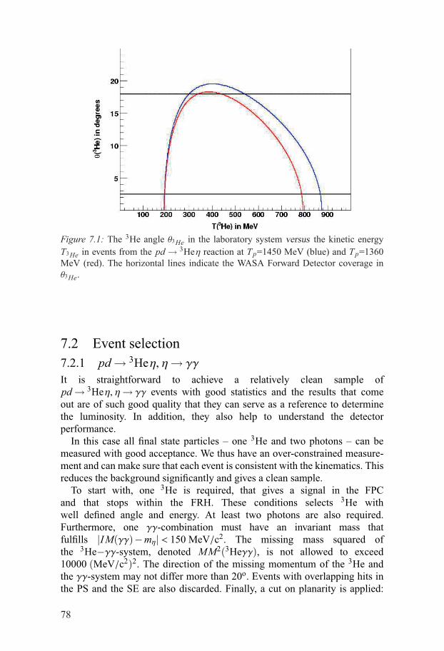
Figure 7.1: The 3He angle θ3He in the laboratory system versus the kinetic energyT3He in events from the pd→ 3Heη reaction at Tp=1450 MeV (blue) and Tp=1360MeV (red). The horizontal lines indicate the WASA Forward Detector coverage inθ3He.

7.2 Event selection7.2.1 pd→ 3Heη, η→ γγ

It is straightforward to achieve a relatively clean sample ofpd→ 3Heη, η→ γγ events with good statistics and the results that comeout are of such good quality that they can serve as a reference to determinethe luminosity. In addition, they also help to understand the detectorperformance.

In this case all final state particles – one 3He and two photons – can bemeasured with good acceptance. We thus have an over-constrained measure-ment and can make sure that each event is consistent with the kinematics. Thisreduces the background significantly and gives a clean sample.

To start with, one 3He is required, that gives a signal in the FPCand that stops within the FRH. These conditions selects 3He withwell defined angle and energy. At least two photons are also required.Furthermore, one γγ-combination must have an invariant mass thatfulfills |IM(γγ)−mη| < 150 MeV/c2. The missing mass squared ofthe 3He−γγ-system, denoted MM2(3Heγγ), is not allowed to exceed10000 (MeV/c2)2. The direction of the missing momentum of the 3He andthe γγ-system may not differ more than 20o. Events with overlapping hits inthe PS and the SE are also discarded. Finally, a cut on planarity is applied:

78

Figure 7.2: The acceptance as a function of cosθ∗η at Tp=1450 MeV (dotted line) andat Tp=1360 MeV (solid line) for the constraints optimised for selection of η→ γγ,given in the text in 7.2.1.

Table 7.1: The constraints applied for selection of pd→3 Heη, η→ γγ

3He giving signal in the FPC and stopping in the FRH� 2 photons in the SEone γγ-combination fulfilling|IM(γγ)−mη| < 150 MeV/c2

MM2(3Heγγ) < 10000 (MeV/c2)2

θ(γγ)mm(3He) < 20o

no overlapping hits in the PS and the SE160o < |φlab(3He)−φlab(γγ)| < 200o

160o < |φlab(3He)−φlab(γγ)| < 200o. The constraints are also summarised intable 7.1.Assuming phase space production, the final acceptance with these constraintsis 20% at Tp = 1360 MeV and 14% at Tp = 1450 MeV. The total acceptanceis model dependent, since a large part of the η angular range is not covered.The total acceptance, integrated over the full cosθ∗η range, is calculated as-suming isotropy which is probably not a realistic assumption. However, whenstudying the angular distributions, the sample is divided into small intervals

79

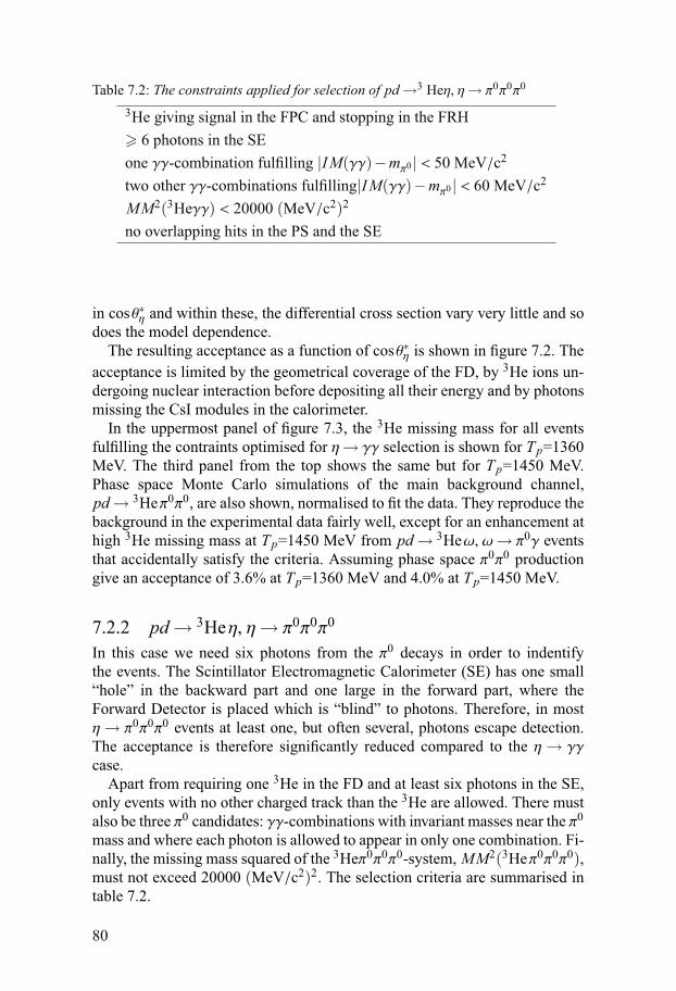
Table 7.2: The constraints applied for selection of pd→3 Heη, η→ π0π0π0

3He giving signal in the FPC and stopping in the FRH� 6 photons in the SEone γγ-combination fulfilling |IM(γγ)−mπ0 | < 50 MeV/c2

two other γγ-combinations fulfilling|IM(γγ)−mπ0 | < 60 MeV/c2

MM2(3Heγγ) < 20000 (MeV/c2)2

no overlapping hits in the PS and the SE

in cosθ∗η and within these, the differential cross section vary very little and sodoes the model dependence.

The resulting acceptance as a function of cosθ∗η is shown in figure 7.2. Theacceptance is limited by the geometrical coverage of the FD, by 3He ions un-dergoing nuclear interaction before depositing all their energy and by photonsmissing the CsI modules in the calorimeter.

In the uppermost panel of figure 7.3, the 3He missing mass for all eventsfulfilling the contraints optimised for η→ γγ selection is shown for Tp=1360MeV. The third panel from the top shows the same but for Tp=1450 MeV.Phase space Monte Carlo simulations of the main background channel,pd→ 3Heπ0π0, are also shown, normalised to fit the data. They reproduce thebackground in the experimental data fairly well, except for an enhancement athigh 3He missing mass at Tp=1450 MeV from pd→ 3Heω, ω→ π0γ eventsthat accidentally satisfy the criteria. Assuming phase space π0π0 productiongive an acceptance of 3.6% at Tp=1360 MeV and 4.0% at Tp=1450 MeV.

7.2.2 pd→ 3Heη, η→ π0π0π0

In this case we need six photons from the π0 decays in order to indentifythe events. The Scintillator Electromagnetic Calorimeter (SE) has one small“hole” in the backward part and one large in the forward part, where theForward Detector is placed which is “blind” to photons. Therefore, in mostη→ π0π0π0 events at least one, but often several, photons escape detection.The acceptance is therefore significantly reduced compared to the η→ γγcase.

Apart from requiring one 3He in the FD and at least six photons in the SE,only events with no other charged track than the 3He are allowed. There mustalso be three π0 candidates: γγ-combinations with invariant masses near the π0

mass and where each photon is allowed to appear in only one combination. Fi-nally, the missing mass squared of the 3Heπ0π0π0-system, MM2(3Heπ0π0π0),must not exceed 20000 (MeV/c2)2. The selection criteria are summarised intable 7.2.

80

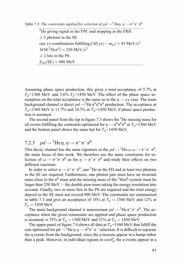
Table 7.3: The constraints applied for selection of pd→3 Heη, η→ π+π−π0

3He giving signal in the FPC and stopping in the FRH� 2 photons in the SEone γγ-combination fulfilling|IM(γγ)−mπ0 | < 45 MeV/c2

MM(3Heπ0) > 250 MeV/c2

� 2 hits in the PSEtot(SE) < 900 MeV

Assuming phase space production, this gives a total acceptance of 5.7% atTp=1360 MeV and 3.6% Tp=1450 MeV. The effect of the phase space as-sumption on the total acceptance is the same as in the η→ γγ case. The mainbackground channel is direct pd→3Heπ0π0π0 production. The acceptance atTp=1360 MeV is 11.7% and 10.3% at Tp=1450 MeV, if phase space produc-tion is assumed.

The second panel from the top in figure 7.3 shows the 3He missing mass forall events fulfilling the contraints optimised for η→ π0π0π0 at Tp=1360 MeVand the bottom panel shows the same but for Tp=1450 MeV.

7.2.3 pd→ 3Heη, η→ π+π−π0

This decay channel has the same signature as the pd→ 3Heω, ω→ π+π−π0,the main focus of this work. We therefore use the same constraints for se-lection of ω→ π+π−π0 as for η→ π+π−π0 and study their effects on twodifferent reactions.

In order to select η→ π+π−π0, one 3He in the FD and at least two photonsin the SE are required. Furthermore, one photon pair must have an invariantmass close to the π0 mass and the missing mass of the 3Heπ0-system must belarger than 250 MeV− the double pion mass taking the energy resolution intoaccount. Finally, two or more hits in the PS are required and the total energydeposit in the SE must not exceed 900 MeV. The constraints are summarisedin table 7.3 and give an acceptance of 18% at Tp = 1360 MeV and 12% atTp = 1450 MeV.

The main background channel is nonresonant pd→ 3Heπ+π−π0. The ac-ceptance when the given constraints are applied and phase space productionis assumed, is 35% at Tp = 1360 MeV and 31% at Tp = 1450 MeV.

The upper panel of figure 7.4 shows all data at Tp=1360 MeV that fulfill thecuts optimised for pd→ 3Heη,η→ π0π+π− selection. It is difficult to separatethe η events from the background, since the η mesons appear in a bump ratherthan a peak. However, in individual regions in cosθ∗η, the η events appear in a

81

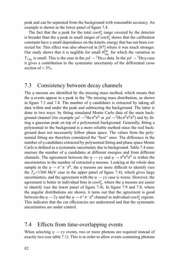
peak and can be separated from the background with reasonable accuracy. Anexample is shown in the lower panel of figure 7.4.

The fact that the η peak for the total cosθ∗η range covered by the detectoris broader than the η peak in small ranges of cosθ∗η shows that the calibrationconstants have a small dependence on the kinetic energy that has not been cor-rected for. This effect was also observed in [87] where it was much stronger.Our study shows that it is neglible for small θlab3He for which the variation inT3He is small. This is the case in the pd→ 3Heω data. In the pd→ 3Heη caseit gives a contribution to the systematic uncertainty of the differential crosssection of < 3%.

7.3 Consistency between decay channelsThe η mesons are identified by the missing mass method, which means thatthe η events appear in a peak in the 3He missing mass distribution, as shownin figure 7.3 and 7.4. The number of η candidates is extracted by taking alldata within and under the peak and subtracting the background. The latter isdone in two ways: by fitting simulated Monte Carlo data of the main back-ground channel (for example pd→3Heπ0π0 or pd→3Heπ0π0π0) and by fit-ting a gaussian peak on top of a polynomial background. Generally, fitting apolynomial to the background is a more reliable method since the real back-ground does not necessarily follow phase space. The values from the poly-nomial fitting are therefore considered the “best” ones. The difference in thenumber of η candidates extracted by polynomial fitting and phase space MonteCarlo is defined as a systematic uncertainty due to background. Table 7.4 sum-marises the number of η candidates at different energies and from differentchannels. The agreement between the η→ γγ and η→ π0π0π0 is within theuncertainties in the number of extracted η mesons. Looking at the whole datasample in the η→ π+π−π0, the η mesons are more difficult to identify (seethe Tp=1360 MeV case in the upper panel of figure 7.4), which gives largeuncertainties, and the agreement with the η→ γγ case is worse. However, theagreement is better in individual bins in cosθ∗η, where the η mesons are easierto identify (see the lower panel of figure 7.4). In figure 7.9 and 7.8, wherethe angular distributions are shown, it turns out that the agreement is goodbetween the η→ 2γ and the η→ π+π−π0 channel in individual cosθ∗η regions.This indicates that the cut efficiencies are understood and that the systematicuncertainties are under control.

7.4 Effects from time-overlapping eventsWhen selecting η→ γγ events, two or more photons are required instead ofexactly two (see table 7.1). This is in order to allow events containing photons

82

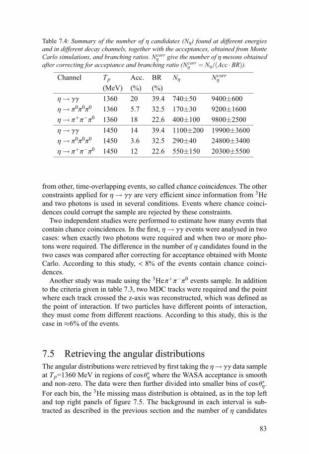
Table 7.4: Summary of the number of η candidates (Nη) found at different energiesand in different decay channels, together with the acceptances, obtained from MonteCarlo simulations, and branching ratios. Ncorrη give the number of η mesons obtainedafter correcting for acceptance and branching ratio (Ncorrη = Nη/(Acc ·BR)).

Channel Tp Acc. BR Nη Ncorrη

(MeV) (%) (%)η→ γγ 1360 20 39.4 740±50 9400±600η→ π0π0π0 1360 5.7 32.5 170±30 9200±1600η→ π+π−π0 1360 18 22.6 400±100 9800±2500η→ γγ 1450 14 39.4 1100±200 19900±3600η→ π0π0π0 1450 3.6 32.5 290±40 24800±3400η→ π+π−π0 1450 12 22.6 550±150 20300±5500

from other, time-overlapping events, so called chance coincidences. The otherconstraints applied for η→ γγ are very efficient since information from 3Heand two photons is used in several conditions. Events where chance coinci-dences could corrupt the sample are rejected by these constraints.

Two independent studies were performed to estimate how many events thatcontain chance coincidences. In the first, η→ γγ events were analysed in twocases: when exactly two photons were required and when two or more pho-tons were required. The difference in the number of η candidates found in thetwo cases was compared after correcting for acceptance obtained with MonteCarlo. According to this study, < 8% of the events contain chance coinci-dences.

Another study was made using the 3Heπ+π−π0 events sample. In additionto the criteria given in table 7.3, two MDC tracks were required and the pointwhere each track crossed the z-axis was reconstructed, which was defined asthe point of interaction. If two particles have different points of interaction,they must come from different reactions. According to this study, this is thecase in ≈6% of the events.

7.5 Retrieving the angular distributionsThe angular distributions were retrieved by first taking the η→ γγ data sampleat Tp=1360 MeV in regions of cosθ∗η where the WASA acceptance is smoothand non-zero. The data were then further divided into smaller bins of cosθ∗η.For each bin, the 3He missing mass distribution is obtained, as in the top leftand top right panels of figure 7.5. The background in each interval is sub-tracted as described in the previous section and the number of η candidates

83

can be estimated. This number is corrected for acceptance and branching ra-tio. The procedure is repeated for the Tp=1450 MeV case, for which someexamples are shown in the two bottom panels of figure 7.5. Finally the wholeprocedure is carried out for the η→ π+π−π0 samples at both energies.

7.6 NormalisationMany experiments use a solid target with a known thickness and a beam cur-rent that is monitored and recorded during the runs when the data are col-lected. The luminosity needed for normalisation can then be calculated fromthese parameters. However, WASA used a pellet target. Then the luminos-ity depends on the pellet rate, the beam current, the pellet thickness and thebeam-pellet overlap. The pellet rate and the beam current are monitored andrecorded during experiment, but the pellet thickness is impossible to measurefor each individual pellet, and the beam-pellet overlap is not constant duringa run or even a cycle of data taking and cannot be measured.

Furthermore, as many as 30% of the events may come from interactionsoutside the target, such as beam-rest gas interactions. This means that the lu-minosity must be calculated from a number of recorded events correspondingto a reaction with a well known cross section.

In PROMICE/WASA, this was done by using quasi-elastic pp-scattering(see for example [140] and [87]). Quasi-elastic pp-scattering was then a goodchoice since the cross section is well known and events from this reactionwere collected with good statistics. However, the higher luminosity achievedby CELSIUS/WASA thanks to the thick pellets, requires dedicated triggers fordifferent reactions, as described in section 4. The 3He data in this work havebeen collected using a different trigger than the quasielastic pp events. Thiswould not be a problem if the trigger efficiencies were well known. However,trigger efficiencies are not straightforward to measure. To obtain reliable crosssections of the pd→ 3Heω reaction, it is desirable to normalise the data usinga reaction whose events can be collected using the same trigger. In this way,the trigger efficiency cancels out.

At both energies, the pd→ 3Heη,η→ γγ data samples are relatively clean.In individual angular bins, the signal-to-background ratio lies between 2 and5. The statistics is quite good and the general quality of the data is rigorouslychecked by comparing with the η→ π0π0π0 and the η→ π+π−π0 channels.Furthermore, the pd→ 3Heη reaction has been studied before at SATURNEwith the SPESIV spectrometer [76] at Tp=1350 MeV and Tp=1450 MeV andthe SPESIII [67] at Tp=1450 MeV. The pd→ 3Heη,η→ γγ data are thereforesuitable for normalisation of the cross sections obtained in this work.

The integrated luminosity L is calculated from:dNdΩ

=dσdΩL ·εtrig (7.1)

84

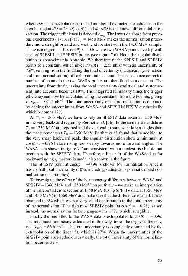
where dN is the acceptance corrected number of extracted η candidates in theangular region dΩ = 2π ·d(cosθ∗η) and dσ/dΩ is the known differential crosssection. The trigger efficiency is denoted εtrig. The larger database from previ-ous experiments ( [76,67]) at Tp = 1450 MeV makes the normalisation proce-dure more straightforward and we therefore start with the 1450 MeV sample.There is a region −1.0 < cosθ∗η <−0.6 where two WASA points overlap witha set of SPESIII and SPESIV points (see figure 7.6). Here, the angular distri-bution is approximately isotropic. We therefore fit the SPESIII and SPESIVpoints to a constant, which gives dσ/dΩ = 2.53 nb/sr with an uncertainty of7.6% coming from the fit taking the total uncertainty (statistical, systematicaland from normalisation) of each point into account. The acceptance correctednumber of counts in the two WASA points are then fitted to a constant. Theuncertainty from the fit, taking the total uncertainty (statistical and systemat-ical) into account, becomes 10%. The integrated luminosity times the triggerefficiency can now be calculated using the constants from the two fits, givingL · εtrig = 381.2 nb−1. The total uncertainty of the normalisation is obtainedby adding the uncertainties from WASA and SPESIII/SPESIV quadraticallywhich becomes 12%.

At Tp = 1360 MeV, we have to rely on SPESIV data taken at 1350 MeVin the very backward region by Berthet et al. [76]. In the same article, data atTp = 1250 MeV are reported and they extend to somewhat larger angles thanthe measurements at Tp = 1350 MeV. Berthet et al. found that in addition tothe very sharp backward peak, the angular distribution show a minimum atcosθ∗η ≈ −0.96 before rising less steeply towards more forward angles. TheWASA data shown in figure 7.7 are consistent with a modest rise but do notoverlap with the SPESIV data. Therefore, a linear fit of the WASA data forbackward going η mesons is made, also shown in the figure.

The SPESIV point at cosθ∗η = −0.96 is chosen for normalisation since ithas a small total uncertainty (10%, including statistical, systematical and nor-malisation uncertainties).

To investigate the effect of the beam energy difference between WASA andSPESIV – 1360 MeV and 1350 MeV, respectively – we make an interpolationof the differential cross section at 1350 MeV (using SPESIV data at 1350 MeVand 1450 MeV) to 1360 MeV and make sure that the difference is small. It wasobtained to 3% which gives a very small contribution to the total uncertaintyof the normalistion. If the rightmost SPESIV point (at cosθ∗η =−0.95) is usedinstead, the normalisation factor changes with 1.5%, which is neglible.

Finally the line fitted to the WASA data is extrapolated to cosθ∗η =−0.96.The integrated luminosity calculated in this way, times the trigger efficiency,is L · εtrig = 66.6 nb−1. The total uncertainty is completely dominated by theextrapolation of the linear fit, which is 27%. When the uncertainties of theSPESIV points are added quadratically, the total uncertainty of the normalisa-tion becomes 29%.

85

Table 7.5: The differential cross section of the pd →3 Heη reaction at Tp = 1360MeV in given intervals of cosθ∗η. The statistical and systematical uncertainties arealso shown. In addition, there is an overall normalisation uncertainty of 29%.

cosθ∗η dσ/dΩ∗η (nb/sr) stat. unc. (nb/sr) syst. unc. (nb/sr)[−0.95 :−0.75] 4.5 1.1 1.4[−0.65 :−0.45] 6.7 1.1 0.8[−0.45 :−0.30] 6.7 1.2 0.6[−0.30 :−0.15] 7.5 0.9 0.6[0.65 : 0.70] 16.1 2.6 1.0[0.70 : 0.80] 23.7 2.4 4.8

7.7 The cross sectionsThe differential cross section at Tp=1360 MeV is shown in figure 7.8 and intable 7.5.The total cross section is obtained by fitting a series of Legendre polynomials

dσdΩ

(cosθ∗ω) =kmax∑k=0akPk(cosθ∗ω) (7.2)

to the η→ γγ data points from WASA. The zeroth coefficient of the Leg-endre polynomial gives, when multiplied with 4π, the total cross section.At Tp = 1360 MeV, a fit with kmax = 2 gives a χ2/ndf of 8.4. When includ-ing the systematical uncertainties in addition to the statistical ones in the fit,χ2/ndf becomes 4.9 but the zeroth coefficient is fairly unchanged – the differ-ence is treated as a systematic uncertainty. This gives a total cross section ofσtot = 151.6±9.3±12.6 nb with an additional uncertainty from the normali-sation of 29%. Since the WASA detector does not cover the full angular range,there is also an unknown uncertainty due to the extrapolation into the region−0.15 < cosθ∗η < 0.65.

The differential cross section at Tp = 1450 MeV as a function of cosθ∗ηis shown in figure 7.9. The normalisation is made using data fulfilling-0.99< cosθ∗η <-0.60 but WASA data agree with SPESIII [67] data also in the-0.6< cosθ∗η <-0.1 interval. In the forward direction there are no overlappingpoints but WASA and SPES3 data seem to disagree significantly. Thedifferential cross section obtained by WASA at Tp = 1450 MeV in the sevenregions of cosθ∗η is also given in table 7.6.The total cross section at Tp = 1450 MeV is calculated in the same way asat 1360 MeV. Only WASA points are included in the fit. Now kmax = 4 givesχ2/ndf of 1.3 and a total cross section σtot = 80.9±3.6±2.5 nb, where thefirst uncertainty is statistical and comes from the fit, while the second comes

86

Table 7.6: The differential cross section of the pd→3Heη reaction at Tp = 1450 MeVin given intervals of cosθ∗η. The statistical and systematical uncertainties are alsoshown. In addition, there is an overall normalisation uncertainty of 12%.

cosθ∗η dσ/dΩ∗η (nb/sr) stat. unc. (nb/sr) syst. unc. (nb/sr)[−0.98 :−0.78] 2.6 0.4 0.1[−0.78 :−0.58] 2.5 0.3 0.1[−0.58 :−0.38] 3.1 0.3 0.1[−0.38 :−0.23] 4.0 0.4 0.02[0.75 : 0.80] 11.8 1.1 2.6[0.80 : 0.85] 13.1 1.3 0.2[0.85 : 0.90] 12.6 1.4 1.6

Table 7.7: The pd→3Heη total cross sections at 1360 MeV and 1450 MeV. In additionto the systematic uncertainty given in the table, there is a normalisation uncertaintyof 29% at 1360 MeV and one of 12% at 1450 MeV.

Tp (MeV) σ (μb) stat. unc. (μb) syst. unc. (μb)1360 0.1516 ±0.0093 ±0.01261450 0.0809 ±0.0036 ±0.0025

from the fit taking the systematic uncertainties into account. Furthermore,there is a normalisation uncertainty of 12% and an unknown uncertainty fromthe extrapolation over the region −0.23 < cosθ∗η < 0.75.

The total cross sections are summarised in table 7.7. Figure 7.10 shows thecross section as a function of p∗η. The WASA data points are at p∗η = 516 MeV/cand p∗η= 568 MeV/c. Data from Mayer et al. [86], Betigeri et al. [88], Banaigset al. [141] and SPESIII [67] are also shown. Recent pd→ 3Heη data nearthreshold from COSY-11 [142] [143] and COSY-ANKE [144] were omittedfrom the graph for the sake of readability but agree with the near-thresholddata in [86].

87

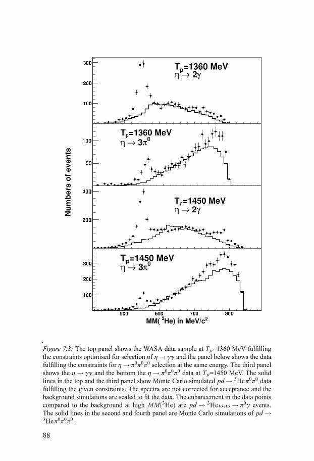
Figure 7.3: The top panel shows the WASA data sample at Tp=1360 MeV fulfillingthe constraints optimised for selection of η→ γγ and the panel below shows the datafulfilling the constraints for η→ π0π0π0 selection at the same energy. The third panelshows the η→ γγ and the bottom the η→ π0π0π0 data at Tp=1450 MeV. The solidlines in the top and the third panel show Monte Carlo simulated pd→ 3Heπ0π0 datafulfilling the given constraints. The spectra are not corrected for acceptance and thebackground simulations are scaled to fit the data. The enhancement in the data pointscompared to the background at high MM(3He) are pd → 3Heω,ω→ π0γ events.The solid lines in the second and fourth panel are Monte Carlo simulations of pd→3Heπ0π0π0.

88

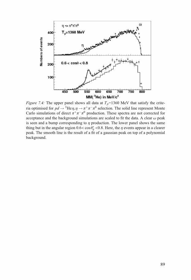
Figure 7.4: The upper panel shows all data at Tp=1360 MeV that satisfy the crite-ria optimised for pd→ 3Heη,η→ π+π−π0 selection. The solid line represent MonteCarlo simulations of direct π+π−π0 production. These spectra are not corrected foracceptance and the background simulations are scaled to fit the data. A clear ω peakis seen and a bump corresponding to η production. The lower panel shows the samething but in the angular region 0.6< cosθ∗η <0.8. Here, the η events appear in a clearerpeak. The smooth line is the result of a fit of a gaussian peak on top of a polynomialbackground.

89

Figure 7.5: The 3He missing mass distribution for events satisfying the constraintsoptimised for η→ γγ selection (see text) in given intervals of cosθ∗η. These MM-spectra are not acceptance corrected and the background simulations are scaled to fitthe data.

90

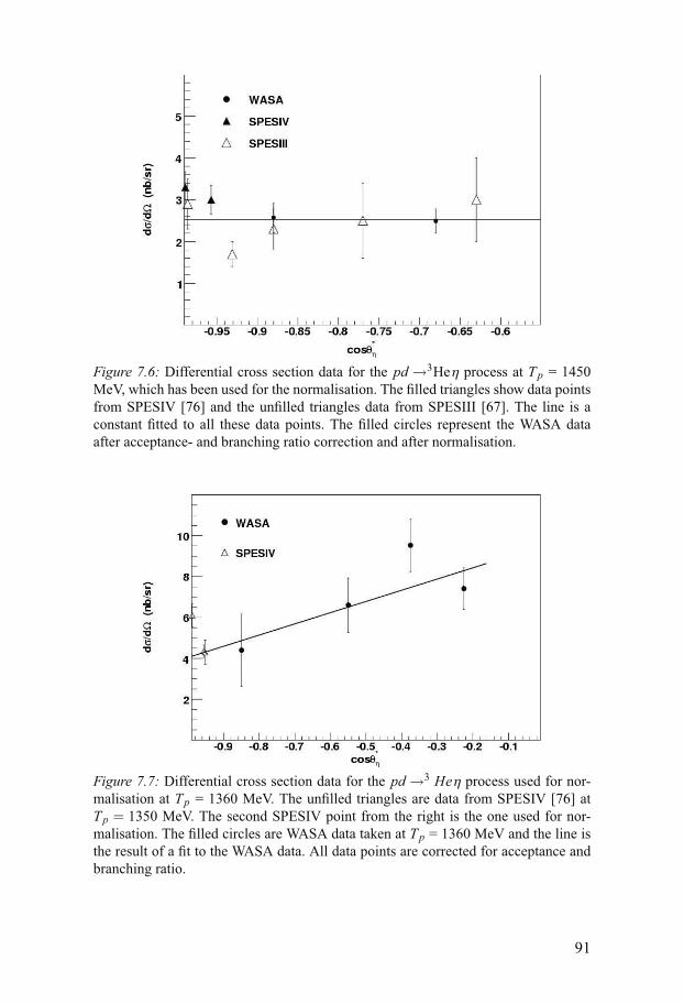
Figure 7.6: Differential cross section data for the pd→3Heη process at Tp = 1450MeV, which has been used for the normalisation. The filled triangles show data pointsfrom SPESIV [76] and the unfilled triangles data from SPESIII [67]. The line is aconstant fitted to all these data points. The filled circles represent the WASA dataafter acceptance- and branching ratio correction and after normalisation.

Figure 7.7: Differential cross section data for the pd→3 Heη process used for nor-malisation at Tp = 1360 MeV. The unfilled triangles are data from SPESIV [76] atTp = 1350 MeV. The second SPESIV point from the right is the one used for nor-malisation. The filled circles are WASA data taken at Tp = 1360 MeV and the line isthe result of a fit to the WASA data. All data points are corrected for acceptance andbranching ratio.

91

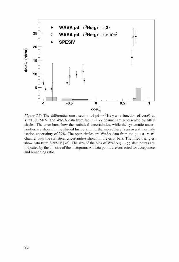
Figure 7.8: The differential cross section of pd → 3Heη as a function of cosθ∗η atTp=1360 MeV. The WASA data from the η→ γγ channel are represented by filledcircles. The error bars show the statistical uncertainties, while the systematic uncer-tainties are shown in the shaded histogram. Furthermore, there is an overall normal-isation uncertainty of 29%. The open circles are WASA data from the η→ π+π−π0

channel with the statistical uncertainties shown in the error bars. The filled trianglesshow data from SPESIV [76]. The size of the bins of WASA η→ γγ data points areindicated by the bin size of the histogram. All data points are corrected for acceptanceand branching ratio.

92

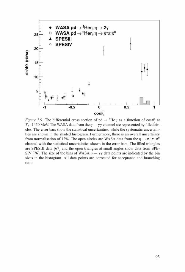
Figure 7.9: The differential cross section of pd → 3Heη as a function of cosθ∗η atTp=1450 MeV. The WASA data from the η→ γγ channel are represented by filled cir-cles. The error bars show the statistical uncertainties, while the systematic uncertain-ties are shown in the shaded histogram. Furthermore, there is an overall uncertaintyfrom normalisation of 12%. The open circles are WASA data from the η→ π+π−π0

channel with the statistical uncertainties shown in the error bars. The filled trianglesare SPESIII data [67] and the open triangles at small angles show data from SPE-SIV [76]. The size of the bins of WASA η→ γγ data points are indicated by the binsizes in the histogram. All data points are corrected for acceptance and branchingratio.

93

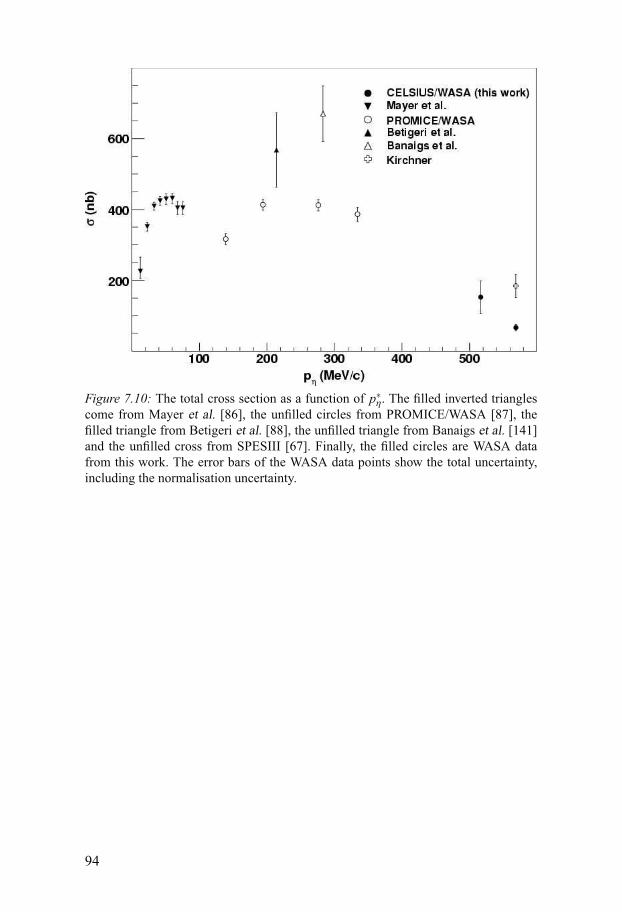
Figure 7.10: The total cross section as a function of p∗η. The filled inverted trianglescome from Mayer et al. [86], the unfilled circles from PROMICE/WASA [87], thefilled triangle from Betigeri et al. [88], the unfilled triangle from Banaigs et al. [141]and the unfilled cross from SPESIII [67]. Finally, the filled circles are WASA datafrom this work. The error bars of the WASA data points show the total uncertainty,including the normalisation uncertainty.

94

8. The pd→ 3Heω reaction

The main subject of this work is production of ω mesons in pd → 3Heω.The two most important decay channels are ω→ π0π+π− (BR = 89.1%) andω→ π0γ (BR = 8.7%). The large ω→ π0π+π− branching ratio gives the largestatistics required for extraction of angular distributions. However, measuringthe ω→ π0γ in parallell provides a valuable consistency check of the results,in particular when we measure the ω polarisation.

8.1 Event selection and acceptance8.1.1 pd→ 3He ω, ω→ π+π−π0

To select ω→ π+π−π0 events, the 3He ion must be measured in the FD withwell defined energy and angle. This requires a signal in at least one of theplanes of the FPC and that the 3He stops within the FRH. The geometricalacceptance of pd→ 3He ω in the FD is, when phase space production is as-sumed, 95% at Tp = 1450 MeV and 78% at Tp = 1360 MeV. The main eventloss is when 3He ions emitted at small laboratory angles escape in the beampipe. The detection efficiency of the FD is further reduced due to nuclear in-teractions in the detector material. The 3He acceptance in pd→ 3He ω in theFD as obtained from Monte Carlo simulations, is 61% at Tp = 1450 MeVand 54% at Tp = 1360 MeV. The FPC efficiency varies during the run pe-riods and is not well reproduced by the Monte Carlo simulations. However,since an FPC signal is required also in the pd→3Heη case, which is used fornormalisation (see section 7.6) the FPC efficiency cancels out.

Furthermore, at least two photons in the SE are required with onephoton-photon combination having an invariant mass that satisfies|IM(γγ)−mπ0)| < 45 MeV/c2. The missing mass of the 3Heπ0-system isrequired to be larger than 250 MeV/c2, i.e. the double pion mass takingthe WASA energy resolution into account. Two or more hits in the PS arerequired. Finally, the total energy deposit in the SE must not exceed 900MeV. The constraints are summarised in table 8.1 and they give an overallacceptance of 34% at Tp = 1360 MeV and 35% at Tp = 1450 MeV. Theacceptance is shown in figure 8.1 as a function of cosθ∗ω at both energies.

95

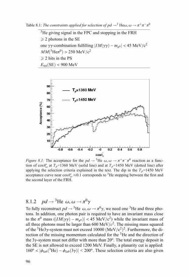
Table 8.1: The constraints applied for selection of pd→3 Heω, ω→ π+π−π0

3He giving signal in the FPC and stopping in the FRH� 2 photons in the SEone γγ-combination fulfilling |IM(γγ)−mπ0 | < 45 MeV/c2

MM(3Heπ0) > 250 MeV/c2

� 2 hits in the PSEtot(SE) < 900 MeV

Figure 8.1: The acceptance for the pd → 3He ω, ω→ π+π−π0 reaction as a func-tion of cosθ∗ω at Tp=1360 MeV (solid line) and at Tp=1450 MeV (dotted line) afterapplying the selection criteria explained in the text. The dip in the Tp=1450 MeVacceptance curve near cosθ∗ω ≈0.1 corresponds to 3He stopping between the first andthe second layer of the FRH.

8.1.2 pd→ 3He ω, ω→ π0γ

To fully reconstruct pd→ 3He ω, ω→ π0γ, we need one 3He and three pho-tons. In addition, one photon pair is required to have an invariant mass closeto the π0 mass (|IM(γγ)−mπ0)| < 45 MeV/c2) while the invariant mass ofall three photons must be larger than 600 MeV/c2. The missing mass squaredof the 3He3γ-system must not exceed 10000 (MeV/c2)2. Furthermore, the di-rection of the missing momentum calculated for the 3He and the direction ofthe 3γ-system must not differ with more than 20o. The total energy deposit inthe SE is not allowed to exceed 1200 MeV. Finally, a planarity cut is applied:160o < |φlab(3He)−φlab(3γ)| < 200o. These selection criteria are also given

96

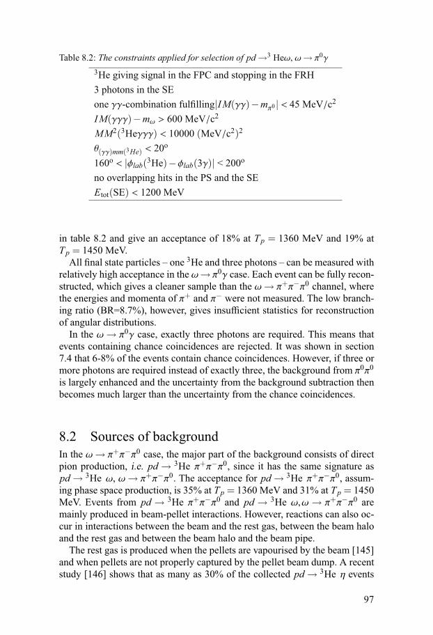
Table 8.2: The constraints applied for selection of pd→3 Heω, ω→ π0γ

3He giving signal in the FPC and stopping in the FRH3 photons in the SEone γγ-combination fulfilling|IM(γγ)−mπ0 | < 45 MeV/c2

IM(γγγ)−mω > 600 MeV/c2

MM2(3Heγγγ) < 10000 (MeV/c2)2

θ(γγ)mm(3He) < 20o

160o < |φlab(3He)−φlab(3γ)| < 200o

no overlapping hits in the PS and the SEEtot(SE) < 1200 MeV

in table 8.2 and give an acceptance of 18% at Tp = 1360 MeV and 19% atTp = 1450 MeV.

All final state particles – one 3He and three photons – can be measured withrelatively high acceptance in the ω→ π0γ case. Each event can be fully recon-structed, which gives a cleaner sample than the ω→ π+π−π0 channel, wherethe energies and momenta of π+ and π− were not measured. The low branch-ing ratio (BR=8.7%), however, gives insufficient statistics for reconstructionof angular distributions.

In the ω→ π0γ case, exactly three photons are required. This means thatevents containing chance coincidences are rejected. It was shown in section7.4 that 6-8% of the events contain chance coincidences. However, if three ormore photons are required instead of exactly three, the background from π0π0

is largely enhanced and the uncertainty from the background subtraction thenbecomes much larger than the uncertainty from the chance coincidences.

8.2 Sources of backgroundIn the ω→ π+π−π0 case, the major part of the background consists of directpion production, i.e. pd → 3He π+π−π0, since it has the same signature aspd→ 3He ω, ω→ π+π−π0. The acceptance for pd→ 3He π+π−π0, assum-ing phase space production, is 35% at Tp = 1360 MeV and 31% at Tp = 1450MeV. Events from pd → 3He π+π−π0 and pd → 3He ω,ω→ π+π−π0 aremainly produced in beam-pellet interactions. However, reactions can also oc-cur in interactions between the beam and the rest gas, between the beam haloand the rest gas and between the beam halo and the beam pipe.

The rest gas is produced when the pellets are vapourised by the beam [145]and when pellets are not properly captured by the pellet beam dump. A recentstudy [146] shows that as many as 30% of the collected pd→ 3He η events

97

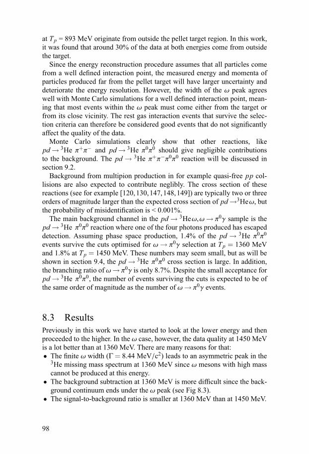
at Tp = 893 MeV originate from outside the pellet target region. In this work,it was found that around 30% of the data at both energies come from outsidethe target.

Since the energy reconstruction procedure assumes that all particles comefrom a well defined interaction point, the measured energy and momenta ofparticles produced far from the pellet target will have larger uncertainty anddeteriorate the energy resolution. However, the width of the ω peak agreeswell with Monte Carlo simulations for a well defined interaction point, mean-ing that most events within the ω peak must come either from the target orfrom its close vicinity. The rest gas interaction events that survive the selec-tion criteria can therefore be considered good events that do not significantlyaffect the quality of the data.

Monte Carlo simulations clearly show that other reactions, likepd→ 3He π+π− and pd→ 3He π0π0 should give negligible contributionsto the background. The pd → 3He π+π−π0π0 reaction will be discussed insection 9.2.

Background from multipion production in for example quasi-free pp col-lisions are also expected to contribute neglibly. The cross section of thesereactions (see for example [120,130,147,148,149]) are typically two or threeorders of magnitude larger than the expected cross section of pd→3Heω, butthe probability of misidentification is < 0.001%.

The main background channel in the pd→ 3Heω,ω→ π0γ sample is thepd→ 3He π0π0 reaction where one of the four photons produced has escapeddetection. Assuming phase space production, 1.4% of the pd → 3He π0π0

events survive the cuts optimised for ω→ π0γ selection at Tp = 1360 MeVand 1.8% at Tp = 1450 MeV. These numbers may seem small, but as will beshown in section 9.4, the pd→ 3He π0π0 cross section is large. In addition,the branching ratio of ω→ π0γ is only 8.7%. Despite the small acceptance forpd→ 3He π0π0, the number of events surviving the cuts is expected to be ofthe same order of magnitude as the number of ω→ π0γ events.

8.3 ResultsPreviously in this work we have started to look at the lower energy and thenproceeded to the higher. In the ω case, however, the data quality at 1450 MeVis a lot better than at 1360 MeV. There are many reasons for that:• The finite ω width (Γ = 8.44 MeV/c2) leads to an asymmetric peak in the

3He missing mass spectrum at 1360 MeV since ω mesons with high masscannot be produced at this energy.

• The background subtraction at 1360 MeV is more difficult since the back-ground continuum ends under the ω peak (see Fig 8.3).

• The signal-to-background ratio is smaller at 1360 MeV than at 1450 MeV.

98

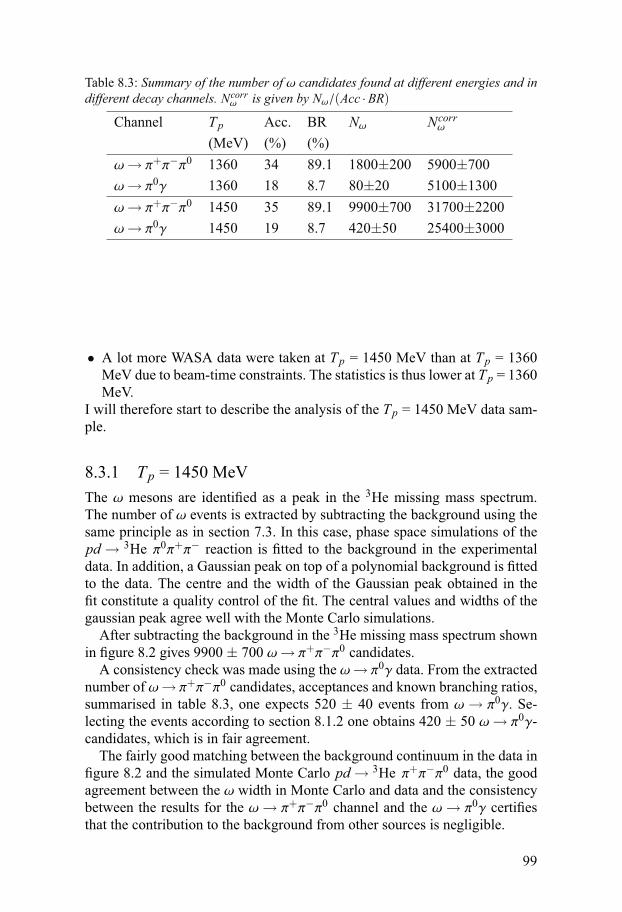
Table 8.3: Summary of the number of ω candidates found at different energies and indifferent decay channels. Ncorrω is given by Nω/(Acc ·BR)

Channel Tp Acc. BR Nω Ncorrω

(MeV) (%) (%)ω→ π+π−π0 1360 34 89.1 1800±200 5900±700ω→ π0γ 1360 18 8.7 80±20 5100±1300ω→ π+π−π0 1450 35 89.1 9900±700 31700±2200ω→ π0γ 1450 19 8.7 420±50 25400±3000

• A lot more WASA data were taken at Tp = 1450 MeV than at Tp = 1360MeV due to beam-time constraints. The statistics is thus lower at Tp = 1360MeV.

I will therefore start to describe the analysis of the Tp = 1450 MeV data sam-ple.

8.3.1 Tp = 1450 MeVThe ω mesons are identified as a peak in the 3He missing mass spectrum.The number of ω events is extracted by subtracting the background using thesame principle as in section 7.3. In this case, phase space simulations of thepd → 3He π0π+π− reaction is fitted to the background in the experimentaldata. In addition, a Gaussian peak on top of a polynomial background is fittedto the data. The centre and the width of the Gaussian peak obtained in thefit constitute a quality control of the fit. The central values and widths of thegaussian peak agree well with the Monte Carlo simulations.

After subtracting the background in the 3He missing mass spectrum shownin figure 8.2 gives 9900 ± 700 ω→ π+π−π0 candidates.

A consistency check was made using the ω→ π0γ data. From the extractednumber of ω→ π+π−π0 candidates, acceptances and known branching ratios,summarised in table 8.3, one expects 520 ± 40 events from ω→ π0γ. Se-lecting the events according to section 8.1.2 one obtains 420 ± 50 ω→ π0γ-candidates, which is in fair agreement.

The fairly good matching between the background continuum in the data infigure 8.2 and the simulated Monte Carlo pd→ 3He π+π−π0 data, the goodagreement between the ω width in Monte Carlo and data and the consistencybetween the results for the ω→ π+π−π0 channel and the ω→ π0γ certifiesthat the contribution to the background from other sources is negligible.

99

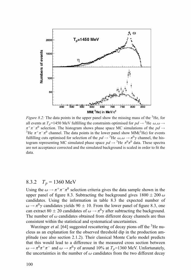
Figure 8.2: The data points in the upper panel show the missing mass of the 3He, forall events at Tp=1450 MeV fulfilling the constraints optimised for pd→ 3He ω,ω→π+π−π0 selection. The histogram shows phase space MC simulations of the pd →3He π+π−π0 channel. The data points in the lower panel show MM(3He) for eventsfulfilling cuts optimised for selection of the pd→ 3He ω,ω→ π0γ channel, the his-togram representing MC simulated phase space pd→ 3He π0π0 data. These spectraare not acceptance corrected and the simulated background is scaled in order to fit thedata.

8.3.2 Tp = 1360 MeVUsing the ω→ π+π−π0 selection criteria gives the data sample shown in theupper panel of figure 8.3. Subtracting the background gives 1800 ± 200 ωcandidates. Using the information in table 8.3 the expected number ofω→ π0γ candidates yields 90 ± 10. From the lower panel of figure 8.3, onecan extract 80 ± 20 candidates of ω→ π0γ after subtracting the background.The number of ω candidates obtained from different decay channels are thusconsistent within the statistical and systematical uncertainties.

Wurzinger et al. [64] suggested rescattering of decay pions off the 3He nu-cleus as an explanation for the observed threshold dip in the production am-plitude (see also section 2.1.2). Their classical Monte Carlo model predictsthat this would lead to a difference in the measured cross section betweenω→ π0π+π− and ω→ π0γ of around 10% at Tp=1360 MeV. Unfortunately,the uncertainties in the number of ω candidates from the two different decay

100

Figure 8.3: The data points in the upper panel show the 3He missing mass for events atTp=1360 MeV fulfilling the constraints optimised for pd→ 3He ω,ω→ π+π−π0 se-lection. The histogram shows phase space MC simulations of the pd→ 3He π+π−π0

channel. The data points in the lower panel show MM(3He) for events fulfilling cutsoptimised for selection of the pd→ 3He ω,ω→ π0γ channel and the histogram rep-resents phase space MC simulated pd→ 3He π0π0 data. These spectra are not accep-tance corrected and the simulated background is scaled in order to fit the data.

channels obtained with WASA are too large (11% for ω→ π+π−π0 and 25%for ω→ π0γ) to test this prediction.

8.4 The ω angular distribution8.4.1 Tp = 1450 MeVTo extract the differential cross section as a function of cosθ∗ω, theω→ π0π+π− data are divided into bins of cosθ∗ω. For each bin, the 3Hemissing mass distribution is plotted − some examples are shown in figure8.4. The number of ω events is extracted by subtracting the backgroundusing the same two methods as for the full sample, i.e by fitting simulatedbackground and by fitting a gaussian sitting on a polynomial, to the data.Since the background does not always follow phase space well, the resultfrom the polynomial fit is considered most reliable and the differencebetween the results from the polynomial fitting and the fitting of the MonteCarlo simulated background is treated as a systematical uncertainty. Theuncertainty from background subtraction is the most important source of

101

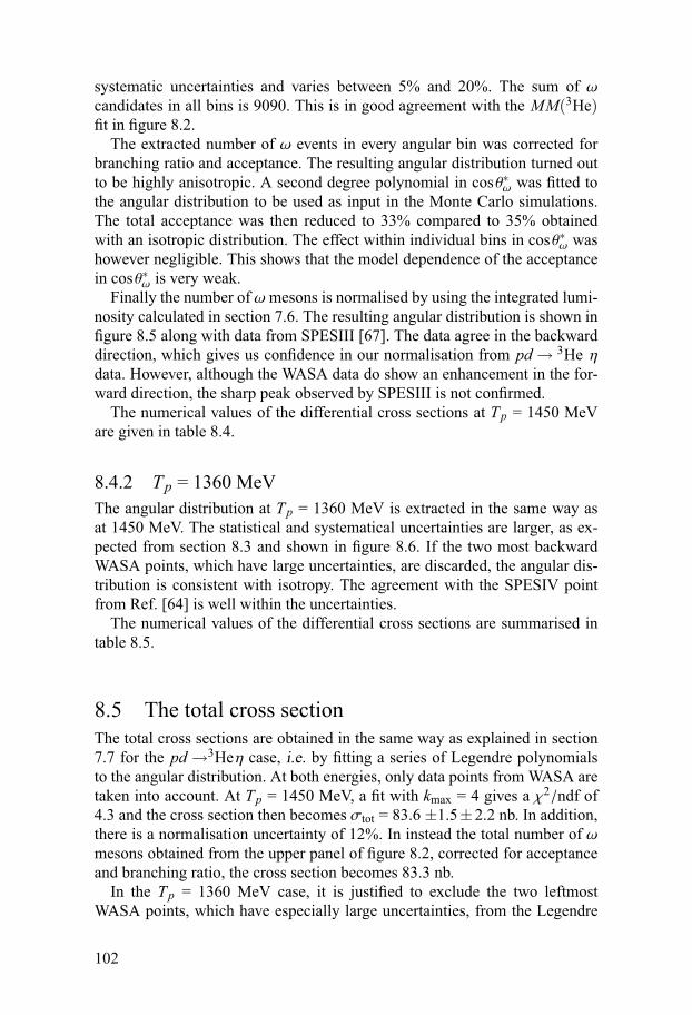
systematic uncertainties and varies between 5% and 20%. The sum of ωcandidates in all bins is 9090. This is in good agreement with the MM(3He)fit in figure 8.2.

The extracted number of ω events in every angular bin was corrected forbranching ratio and acceptance. The resulting angular distribution turned outto be highly anisotropic. A second degree polynomial in cosθ∗ω was fitted tothe angular distribution to be used as input in the Monte Carlo simulations.The total acceptance was then reduced to 33% compared to 35% obtainedwith an isotropic distribution. The effect within individual bins in cosθ∗ω washowever negligible. This shows that the model dependence of the acceptancein cosθ∗ω is very weak.

Finally the number of ω mesons is normalised by using the integrated lumi-nosity calculated in section 7.6. The resulting angular distribution is shown infigure 8.5 along with data from SPESIII [67]. The data agree in the backwarddirection, which gives us confidence in our normalisation from pd→ 3He ηdata. However, although the WASA data do show an enhancement in the for-ward direction, the sharp peak observed by SPESIII is not confirmed.

The numerical values of the differential cross sections at Tp = 1450 MeVare given in table 8.4.

8.4.2 Tp = 1360 MeVThe angular distribution at Tp = 1360 MeV is extracted in the same way asat 1450 MeV. The statistical and systematical uncertainties are larger, as ex-pected from section 8.3 and shown in figure 8.6. If the two most backwardWASA points, which have large uncertainties, are discarded, the angular dis-tribution is consistent with isotropy. The agreement with the SPESIV pointfrom Ref. [64] is well within the uncertainties.

The numerical values of the differential cross sections are summarised intable 8.5.

8.5 The total cross sectionThe total cross sections are obtained in the same way as explained in section7.7 for the pd→3Heη case, i.e. by fitting a series of Legendre polynomialsto the angular distribution. At both energies, only data points from WASA aretaken into account. At Tp = 1450 MeV, a fit with kmax = 4 gives a χ2/ndf of4.3 and the cross section then becomes σtot = 83.6 ±1.5±2.2 nb. In addition,there is a normalisation uncertainty of 12%. In instead the total number of ωmesons obtained from the upper panel of figure 8.2, corrected for acceptanceand branching ratio, the cross section becomes 83.3 nb.

In the Tp = 1360 MeV case, it is justified to exclude the two leftmostWASA points, which have especially large uncertainties, from the Legendre

102

Table 8.4: The differential cross section of the pd→3 Heω reaction at Tp = 1450 MeVin given intervals of cosθ∗ω. The statistical and systematical uncertainties are given.In addition,there is an overall normalisation uncertainty of 12%.

cosθ∗ω dσ/dΩ∗ω (nb/sr) stat. unc. (nb/sr) syst. unc. (nb/sr)[−0.95 :−0.90] 12.4 1.3 1.4[−0.90 :−0.80] 8.6 0.7 0.8[−0.80 :−0.70] 8.4 0.7 0.1[−0.70 :−0.60] 8.1 0.6 2.1[−0.60 :−0.50] 6.8 0.6 0.8[−0.50 :−0.40] 6.4 0.6 0.9[−0.40 :−0.20] 6.3 0.4 1.7[−0.20 : 0.00] 6.0 0.4 1.6[0.00 : 0.20] 4.8 0.3 0.7[0.20 : 0.40] 4.7 0.3 0.5[0.40 : 0.60] 5.0 0.3 1.9[0.60 : 0.70] 6.6 0.5 0.4[0.70 : 0.80] 7.0 0.6 2.1[0.80 : 0.85] 7.0 0.8 1.7[0.85 : 0.90] 8.3 0.9 0.4[0.90 : 0.95] 8.6 0.8 1.5

Table 8.5: The differential cross section of the pd→3 Heω reaction at Tp = 1360 MeVin given intervals of cosθ∗ω. The statistical and systematical uncertainties are given.There is also an overall normalisation uncertainty of 29%.

cosθ∗ω dσ/dΩ∗ω (nb/sr) stat. unc. (nb/sr) syst. unc. (nb/sr)[−0.8 :−0.6] 12.4 1.6 7.5[−0.6 :−0.5] 12.3 2.3 4.7[−0.5 :−0.4] 6.6 1.8 3.7[−0.4 :−0.3] 8.3 1.6 2.0[−0.3 :−0.2] 6.2 1.5 2.3[−0.2 : 0.0] 7.0 0.9 1.5[0.0 : 0.2] 6.3 0.8 3.8[0.2 : 0.4] 5.8 0.8 0.9[0.4 : 0.6] 5.6 0.7 1.9[0.6 : 0.8] 6.1 0.7 1.7

103

Table 8.6: The pd→3Heω total cross sections at 1360MeV and 1450MeV. In additionto the systematic uncertainty given in the table, there is a normalisation uncertaintyof 29% at 1360 MeV and one of 12% at 1450 MeV.

Tp (MeV) σ (μb) stat. unc. (μb) syst. unc. (μb)1360 0.0846 ±0.0040 ±0.00481450 0.0836 ±0.0015 ±0.0022

fit. With kmax = 1, one gets a χ2/ndf of 2.3 and the total cross section yieldsσtot = 84.6 ±4.0±4.8 nb. The first uncertainty comes from the fit when onlystatistical uncertainties are taken into account. The second uncertainty is alsofrom the fit, but taking also the systematic uncertainties into account. If thetotal cross section is calculated using the number of events obtained from theupper panel of figure 8.3, the total cross section becomes 89.2 nb. The nor-malisation uncertainty is 29%. The total cross sections of ω production aresummarised in table 8.6.

8.6 Data versus model calculationsThe predictions of the differential cross sections as functions of cosθ∗ω, ob-tained using the two-step model presented in section 2.2, are shown togetherwith experimental data in figure 8.6 in the previous section and in figure 8.7in this section.

At 1360 MeV, the model underpredicts the data with about an order of mag-nitude, as shown in figure 8.6. The data are consistent with isotropy but theuncertainties are too large to test whether the model, that predicts a small for-ward enhancement, reproduce the shape.

At 1450 MeV, the two-step model fails to describe the shape of the angulardistribution. The discrepancy is largest at very large and very small angles:the model predicts a suppressed cross section there while the data show strongrises. This is shown in figure 8.7

It should be noted that if only s-waves are included in the πN→ Nω vertexin the calculations (see figure 2.3 in section 2.2), the discrepancy betweentheory and data is even larger.

In figure 8.8, the total cross section is shown as a function of the beamkinetic energy. The line represents model calculations including partial wavesup to l= 3 and the data points come from this work. The total cross section isunderpredicted by a factor 10 at 1360 MeV and a factor 2 at 1450 MeV.

104

8.7 The polarisation of the ωIt is not only the cross section and the angular distribution of the ω that giveinformation about its production mechanism, but also its polarisation (spinalignment). Being a spin-one meson, theω could either be produced polarised,i.e. with its spin axis in some prefered direction, or unpolarised.

In a recent work from the MOMO collaboration [107], the φ meson inpd→3Heφ, φ→ K+K− was studied. The K+ and K− were measured in co-incidence with the 3He and the angular distribution of the K+K− relative mo-mentum in the rest frame of the φ was studied. In the φ case, the angle be-tween the K+K− relative momentum and some quantisation axis, for examplethe direction of the incoming beam, is sensitive to the tensor polarisation. TheMOMO experiment showed that the φ meson is produced almost completelypolarised, in a magnetic sub-state m = 0 along the beam direction. Recall-ing section 2.4, a comparison between φ and ω production is very valuablesince any differences in the tensor polarisation could mean that the produc-tion mechanisms are different and depend on meson and nucleon degrees offreedom rather than on hadron properties at the quark level.

8.7.1 The Gottfried-Jackson angleFor an ω meson decaying into π+π−π0, the polarisation axis is directed alongthe normal to the decay plane. The polarisation can be measured by studyingthe angle between this normal and some quantisation axis. In the Gottfried-Jackson frame [150] the angle is taken between the normal and the incomingbeam, all in the rest system of theω. The Gottfried-Jackson angle is illustratedin figure 8.9 and will from now on be refered to as β.

We are interested in the elements of the spin-density matrix ρmm′ , whichwas presented in section 2.4. With the unpolarised CELSIUS beam and theunpolarised pellet target, there is one independent element ρ00 = 1− 2ρ11 =1− 2ρ−1−1 to measure. The ρ00 element appears in the expression for thedifferential cross section, given in equation 2.12 in section 2.4. Expressed asa function of the Gottfried-Jackson angle β it reads:

dσ(ω→ π0π+π−)dcosβ

∝ (1−ρ00)+(3ρ00−1)cos2 β. (8.1)

If the ω mesons are unpolarised, then ρ00 = ρ11 = ρ−1−1 = 13 and the distri-

bution of the Gottfried-Jackson angle is isotropic.In section 2.4 it was also mentioned that the ω polarisation can be studied

in the ω→ π0γ decay. The angle is then taken between the π0 or the γ in the ωrest frame and the direction of the incoming beam. This angle is here referedto as β′ and the angular distribution has the form

dσ(ω→ π0γ)dcosβ′

∝ (1+ρ00)− (3ρ00−1)cos2 β′ . (8.2)

105

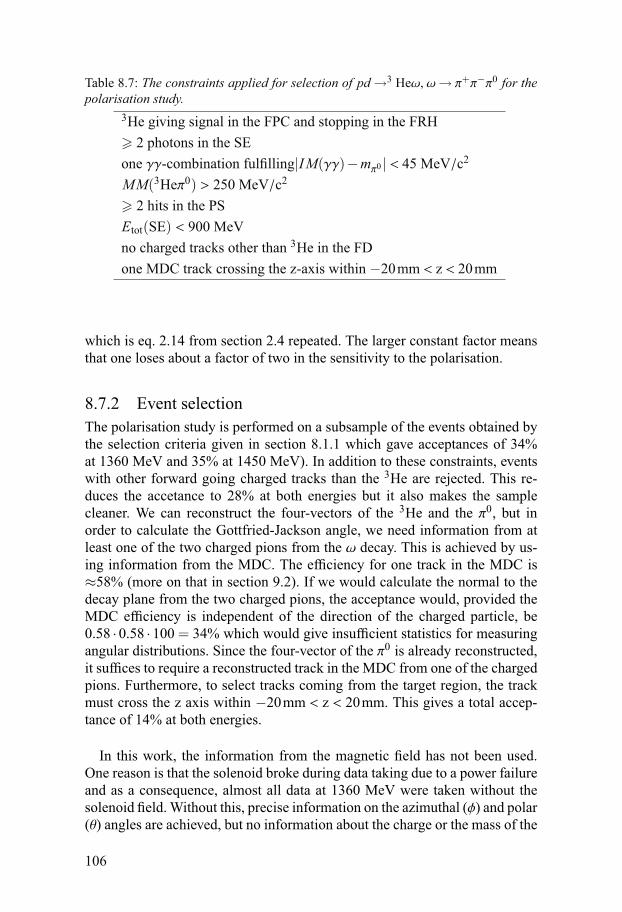
Table 8.7: The constraints applied for selection of pd→3 Heω, ω→ π+π−π0 for thepolarisation study.

3He giving signal in the FPC and stopping in the FRH� 2 photons in the SEone γγ-combination fulfilling|IM(γγ)−mπ0 | < 45 MeV/c2

MM(3Heπ0) > 250 MeV/c2

� 2 hits in the PSEtot(SE) < 900 MeVno charged tracks other than 3He in the FDone MDC track crossing the z-axis within −20mm < z < 20mm

which is eq. 2.14 from section 2.4 repeated. The larger constant factor meansthat one loses about a factor of two in the sensitivity to the polarisation.

8.7.2 Event selectionThe polarisation study is performed on a subsample of the events obtained bythe selection criteria given in section 8.1.1 which gave acceptances of 34%at 1360 MeV and 35% at 1450 MeV). In addition to these constraints, eventswith other forward going charged tracks than the 3He are rejected. This re-duces the accetance to 28% at both energies but it also makes the samplecleaner. We can reconstruct the four-vectors of the 3He and the π0, but inorder to calculate the Gottfried-Jackson angle, we need information from atleast one of the two charged pions from the ω decay. This is achieved by us-ing information from the MDC. The efficiency for one track in the MDC is≈58% (more on that in section 9.2). If we would calculate the normal to thedecay plane from the two charged pions, the acceptance would, provided theMDC efficiency is independent of the direction of the charged particle, be0.58 ·0.58 ·100 = 34% which would give insufficient statistics for measuringangular distributions. Since the four-vector of the π0 is already reconstructed,it suffices to require a reconstructed track in the MDC from one of the chargedpions. Furthermore, to select tracks coming from the target region, the trackmust cross the z axis within −20mm < z < 20mm. This gives a total accep-tance of 14% at both energies.

In this work, the information from the magnetic field has not been used.One reason is that the solenoid broke during data taking due to a power failureand as a consequence, almost all data at 1360 MeV were taken without thesolenoid field. Without this, precise information on the azimuthal (φ) and polar(θ) angles are achieved, but no information about the charge or the mass of the

106

particle. We therefore have to assume that the track is caused by a charged pionand reconstruct its four-vector by using its φ and θ angles obtained from theMDC and by using the known four-vectors of the π0 and the 3He, as shownin the Appendix. The normal of the decay plane is then given by the crossproduct of the π0 and π± momentum three-vectors.

When studying β′ from equation 8.2, events are used that have been selectedwith the criteria presented in table 8.2 of section 8.1.2 optimised for ω→ π0γselection. As previously mentioned, they give an acceptance of 18% at 1360MeV and 19% at 1450 MeV.

8.7.3 ResultsIn figure 8.10, the missing mass distribution of the 3He is shown for threecases: in panel a) ω→ π+π−π0 data at 1450 MeV, in panel b) ω→ π0γ dataat 1450 MeV and in panel c) ω→ π+π−π0 data at 1360 MeV. These sampleshave been used for reconstruction of the β and β′ distributions. The number ofω→ π0γ candidates at 1360 MeV is unfortunately insufficient for a study ofβ′ at this energy.

8.7.3.1 Tp = 1450 MeVIn order to obtain the differential cross section as a function of cos2 β, all theevents fulfilling the given selection criteria were divided into eight regions of|cosβ|. After that, we use the same procedure as when the angular distributionof the ω was retrieved, as described in section 8.4.1; in each region of |cosβ|,a 3He missing mass spectrum was obtained with the ω candidates appearingin a peak. The background under the ω peak was estimated both by takinga phase-space Monte Carlo simulation of pd→ 3Heπ+π−π0 and by fitting agaussian peak sitting on a polynomial background, to the data. The ratio of theω to background over the peak is about 1 : 3 and the difference in the numbersof ω obtained in the two ways is between 2% and 15%. The number of ω can-didates in each region is then corrected for acceptance and normalised by anoverall arbitrary factor to give an average value of unity. The absolute normal-isation based on the integrated luminosity is not relevant when studying thepolarisation, since equations 8.1 and 8.2 only give proportionality relations.The result is shown as filled circles in figure 8.11. The data are clearly consis-tent with isotropy. However, we would like to determine the significance byperforming the same analysis using data that do not contain anyωmesons. Wethen take events from the same sample, shown in figure 8.10 a), divide it intothe same regions in |cosβ| as before, but this time we select events comingfrom outside the peak region, i.e. fulfilling 700 < MM(3He) < 750 MeV/c2.These events are non-resonant pd→3 Heπ+π−π0 events and should give anisotropic distribution. The corresponding points are shown as filled trianglesin figure 8.11. The statistics here are high and there is indeed no sign of any

107

angular dependence. This gives some confidence that our setup and analysisdoes not introduce an artificial angular dependence in the ω case.

In the ω→ π0γ case, the statistics allows us to divide the data into fiveregions in |cosβ′|. The number of ω candidates in each region was again ob-tained by plotting the missing mass of the 3He and subtracting the background,both by using fitted Monte Carlo simulations of pd→ 3Heπ0π0 which is themain background channel (see section 8.2), and by fitting a gaussian peak plusa polynomial. The differences in this case varies between 2% and 25%. Aftercorrecting for acceptance, branching ratio and bin size, we normalise usingthe identical factor to that employed in the ω→ π0π+π− case. The resultingpoints are shown as unfilled circles in figure 8.11 and the good agreement innormalisation between the two decay channels indicates that the relative cutefficiencies and other systematic effects are well understood.

The angular dependence of the ω→ π0π+π− data shown at 1450 MeV infigure 8.11 has been fitted by a straight line to extract the values of ρ00 inEq. (8.1). In this way we obtain ρ00 = 0.33± 0.05 at 1450 MeV. The uncer-tainty here is statistical but it is clear that any deviation from an unpolarisedvalue of 1

3 must be quite small. This is confirmed through the study of theω→ π0γ data, which gives ρ00 = 0.14± 0.14. The statistical uncertainty ofthe fit comes in part from the data uncertainty in each bin, in part from thelower number of bins and in part from the larger constant term in Eq. (8.2)compared to Eq. (8.1), which makes the β′ less sensitive to polarisation thanthe β.

In H.A. Schnitker’s Ph. D. thesis [151], where φ production with MOMOwas studied, it was found that the φ polarisation was highly dependent on the φproduction angle. For cosθ∗φ >−0.5, the distribution of the Gottfried-Jacksonangle was isotropic, while most polarised events were found in the very back-ward region, cosθ∗φ <−0.8. In order to test whether theω polarisation dependsupon its production angle θ∗ω in the overall CM system, the ω→ π+π−π0 dataat 1450 MeV were divided into three sub-samples with respect to cosθ∗ω. Inall three regions the results were consistent with ω being unpolarised.

cosθ∗ω <−0.5 ⇒ ρ00 = 0.29±0.08,|cosθ∗ω| < 0.5 ⇒ ρ00 = 0.37±0.06,cosθ∗ω > 0.5 ⇒ ρ00 = 0.30±0.09.

8.7.3.2 Tp = 1360 MeVFor reasons discussed in section 8.3, the analysis is more difficult at Tp =1360 MeV than at Tp = 1450 MeV which gives larger statistical and system-atical uncertainties. In the event sample shown in figure 8.10 the signal-to-background ratio within 750 < MM(3He) < 800 MeV/c2 is 1 : 5 compared to1 : 3 in the 1450 MeV case.

The statistics now allow for a division of the ω→ π0π+π− data into onlyfive regions of |cosβ| but, apart from this, the procedure for extracting the

108

differential cross section, shown as a function of cos2 β in Fig. 8.12, is exactlythe same as that at 1450 MeV. The systematic uncertainties from backgroundsubtraction are between 18% and 30%. The result is shown as filled circlesin figure 8.12. Within the much larger error bars, the data are consistent withisotropy. Fitting the data to a straight line and using equation 8.1 one obtainsρ00 = 0.34±0.10. The three-pion background, selected in the same way as inthe 1450 MeV case, i.e. by requiring 700 < MM(3He) < 750 MeV/c2, is alsoisotropic in β.

The statistics is insufficient for a consistency check using ω→ π0γ data.Instead the angle between the π0 from the ω→ π0π+π− decay and the incom-ing proton is analysed. Recalling section 2.4, the distribution is then describedby the same experssion as in Eq. (8.2). The sensitivity to the polarisation isthe reduced by a factor of two due to the smaller constant factor in the equa-tion. The angular distribution of the π0 was retrieved at both energies and areisotropic in both cases. The differential cross section as a function of cosβ′2at 1360 MeV, is shown in figure 8.13.

8.7.3.3 The helicity angleIt is also interesting to study the polarisation in the helicity frame [150], wherethe reference axis is provided by the direction of the 3He. Here, we have anal-ysed the angle between the normal of the ω decay plane and the 3He direc-tion in the ω rest system. Unlike the Gottfried-Jackson angle distribution, thiscross section must be flat near threshold since only s-waves can contribute.Although the sensitivity to the polarisation is small, it is reassuring that thehelicity distribution is completely consistent with isotropy at both beam ener-gies. This is shown in figure 8.14.

109

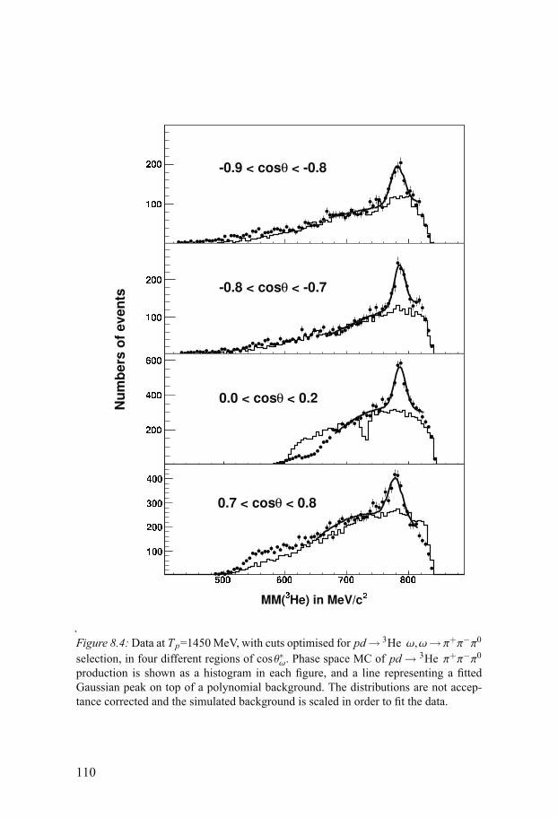
Figure 8.4:Data at Tp=1450 MeV, with cuts optimised for pd→ 3He ω,ω→ π+π−π0

selection, in four different regions of cosθ∗ω. Phase space MC of pd→ 3He π+π−π0

production is shown as a histogram in each figure, and a line representing a fittedGaussian peak on top of a polynomial background. The distributions are not accep-tance corrected and the simulated background is scaled in order to fit the data.

110

Figure 8.5: Comparison of WASA pd→3He ω data at Tp = 1450 MeV (filled circles)with SPESIII data [67] (triangles). The vertical error bars on the WASA data show thestatistical uncertainties and the shaded histogram shows the systematical uncertaintydue to background subtraction and acceptance correction. The size of the individualangular bins are indicated by the histogram. Apart from the uncertainties given in thebars and the histogram there is an overall normalisation uncertainty of 12%. All datapoints are corrected for acceptance and branching ratio.

111

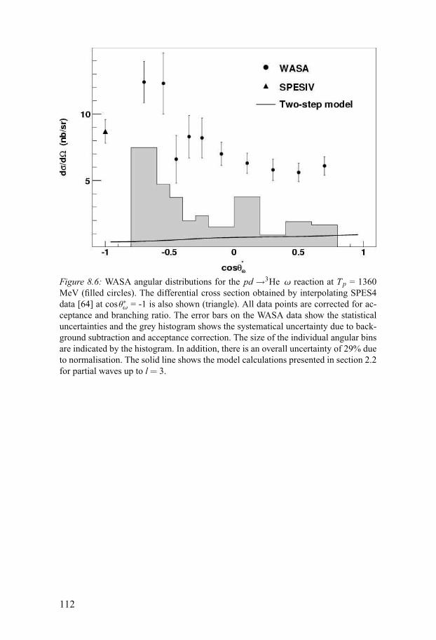
Figure 8.6: WASA angular distributions for the pd→3He ω reaction at Tp = 1360MeV (filled circles). The differential cross section obtained by interpolating SPES4data [64] at cosθ∗ω = -1 is also shown (triangle). All data points are corrected for ac-ceptance and branching ratio. The error bars on the WASA data show the statisticaluncertainties and the grey histogram shows the systematical uncertainty due to back-ground subtraction and acceptance correction. The size of the individual angular binsare indicated by the histogram. In addition, there is an overall uncertainty of 29% dueto normalisation. The solid line shows the model calculations presented in section 2.2for partial waves up to l= 3.

112

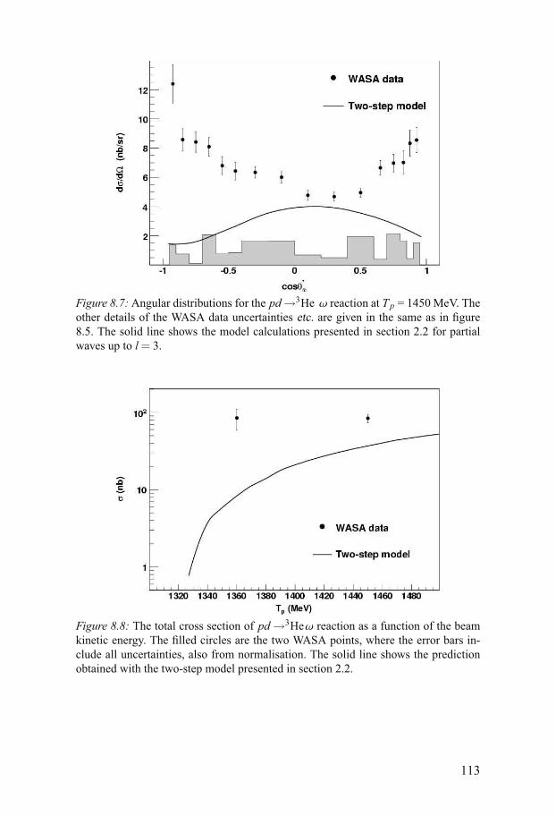
Figure 8.7: Angular distributions for the pd→3He ω reaction at Tp = 1450 MeV. Theother details of the WASA data uncertainties etc. are given in the same as in figure8.5. The solid line shows the model calculations presented in section 2.2 for partialwaves up to l= 3.

Figure 8.8: The total cross section of pd→3Heω reaction as a function of the beamkinetic energy. The filled circles are the two WASA points, where the error bars in-clude all uncertainties, also from normalisation. The solid line shows the predictionobtained with the two-step model presented in section 2.2.

113

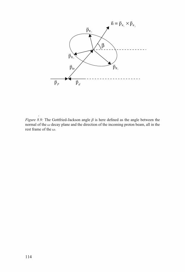
rpp

rpd

rpω

rpπ 1

rpπ 3

rn�=�

rpπ i

×rpπ j

rpπ 2

β

Figure 8.9: The Gottfried-Jackson angle β is here defined as the angle between thenormal of the ω decay plane and the direction of the incoming proton beam, all in therest frame of the ω.

114

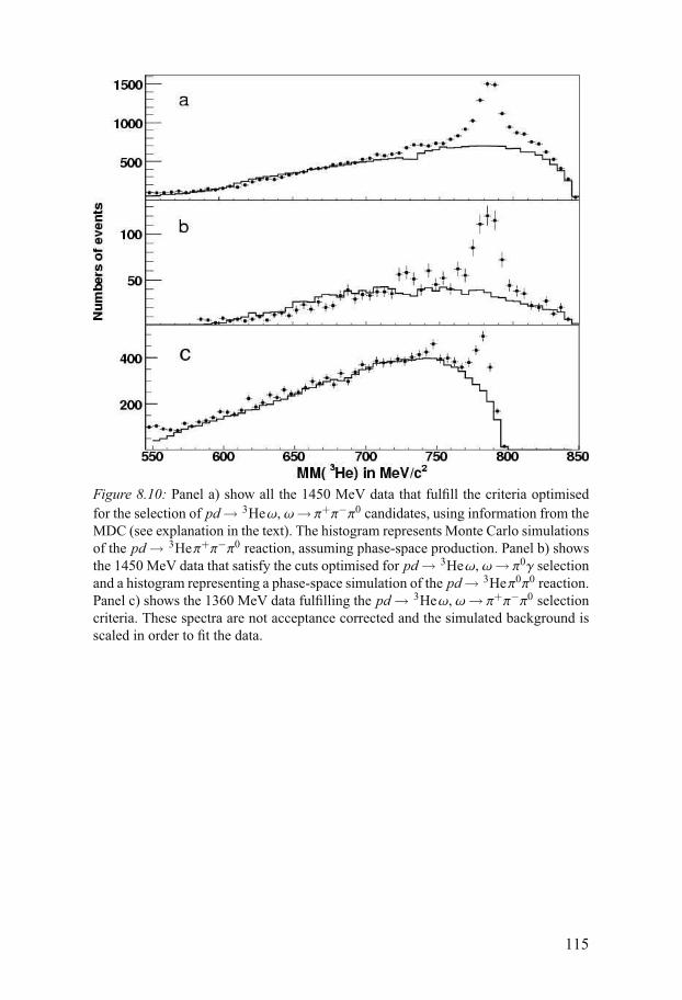
Figure 8.10: Panel a) show all the 1450 MeV data that fulfill the criteria optimisedfor the selection of pd→ 3Heω, ω→ π+π−π0 candidates, using information from theMDC (see explanation in the text). The histogram represents Monte Carlo simulationsof the pd→ 3Heπ+π−π0 reaction, assuming phase-space production. Panel b) showsthe 1450 MeV data that satisfy the cuts optimised for pd→ 3Heω, ω→ π0γ selectionand a histogram representing a phase-space simulation of the pd→ 3Heπ0π0 reaction.Panel c) shows the 1360 MeV data fulfilling the pd→ 3Heω, ω→ π+π−π0 selectioncriteria. These spectra are not acceptance corrected and the simulated background isscaled in order to fit the data.

115

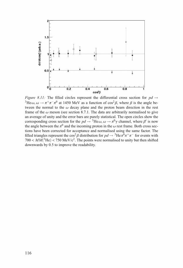
Figure 8.11: The filled circles represent the differential cross section for pd →3Heω, ω→ π+π−π0 at 1450 MeV as a function of cos2 β, where β is the angle be-tween the normal to the ω decay plane and the proton beam direction in the restframe of the ω meson (see section 8.7.1. The data are arbitrarily normalised to givean average of unity and the error bars are purely statistical. The open circles show thecorresponding cross section for the pd→ 3Heω, ω→ π0γ channel, where β′ is nowthe angle between the π0 and the incoming proton in the ω rest frame. Both cross sec-tions have been corrected for acceptance and normalised using the same factor. Thefilled triangles represent the cos2 β distribution for pd→ 3Heπ0π+π− for events with700 < MM(3He) < 750 MeV/c2. The points were normalised to unity but then shifteddownwards by 0.5 to improve the readability.

116

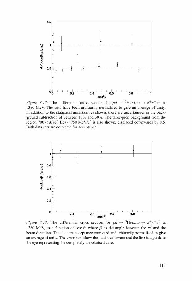
Figure 8.12: The differential cross section for pd → 3Heω, ω → π+π−π0 at1360 MeV. The data have been arbitrarily normalised to give an average of unity.In addition to the statistical uncertainties shown, there are uncertainties in the back-ground subtraction of between 18% and 30%. The three-pion background from theregion 700 < MM(3He) < 750 MeV/c2 is also shown, displaced downwards by 0.5.Both data sets are corrected for acceptance.

Figure 8.13: The differential cross section for pd → 3Heω,ω → π+π−π0 at1360 MeV, as a function of cos2 β′ where β′ is the angle between the π0 and thebeam direction. The data are acceptance corrected and arbitrarily normalised to givean average of unity. The error bars show the statistical errors and the line is a guide tothe eye representing the completely unpolarised case.

117

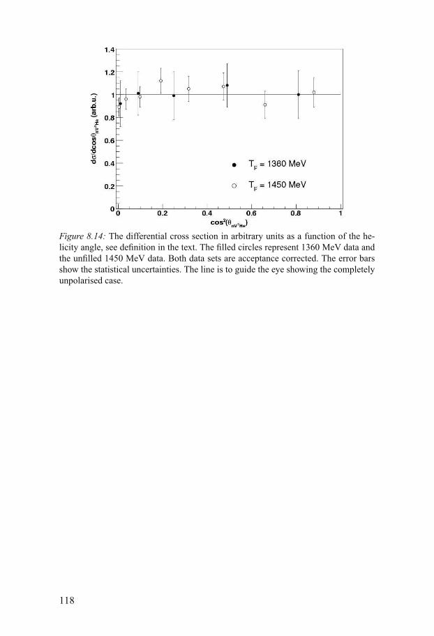
Figure 8.14: The differential cross section in arbitrary units as a function of the he-licity angle, see definition in the text. The filled circles represent 1360 MeV data andthe unfilled 1450 MeV data. Both data sets are acceptance corrected. The error barsshow the statistical uncertainties. The line is to guide the eye showing the completelyunpolarised case.

118

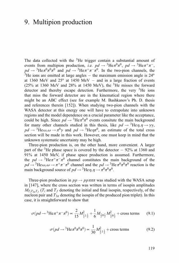
9. Multipion production

The data collected with the 3He trigger contain a substantial amount ofevents from multipion production, i.e. pd → 3Heπ0π0, pd → 3Heπ+π−,pd → 3Heπ0π0π0 and pd → 3Heπ+π−π0. In the two-pion channels, the3He ions are emitted at large angles − the maximum emission angle is 24o

at 1360 MeV and 25o at 1450 MeV − and in a large fraction of events(25% at 1360 MeV and 28% at 1450 MeV), the 3He misses the forwarddetector and thereby escape detection. Furthermore, the very 3He ionsthat miss the forward detector are in the kinematical region where theremight be an ABC effect (see for example M. Bashkanov’s Ph. D. thesisand references therein [152]). When studying two-pion channels with theWASA detector at this energy one will have to extrapolate into unknownregions and the model dependence on a crucial parameter like the acceptance,could be high. Since pd → 3Heπ0π0 events consitute the main backgroundfor many other channels studied in this thesis, like pd → 3Heη,η→ γγ,pd → 3Heω,ω→ π0γ and pd → 3Heηπ0, an estimate of the total crosssection will be made in this work. However, one must keep in mind that theunknown systematic uncertainty may be high.

Three-pion production is, on the other hand, more convenient. A largerpart of the 3He phase space is covered by the detector − 92% at 1360 and91% at 1450 MeV, if phase space production is assumed. Furthermore,the pd → 3Heπ+π−π0 channel constitutes the main background of thepd→ 3Heω,ω→ π+π−π0 channel and the pd→ 3He π0π0π0 reaction is themain background source of pd→ 3Heη,η→ π0π0π0.

Three-pion production in pp→ ppπππ was studied with the WASA setupin [147], where the cross section was written in terms of isospin amplitudesMTiT3πT f (Ti and T f denoting the initial and final isospin, respectively, of thenucleon pair and T3π denoting the isospin of the produced pion triplet). In thiscase, it is straightforward to show that

σ(pd→ 3Heπ+π−π0) ∝2

15M2

12 1 1

2+

16M 1

2 0 12M2

12 0 1

2+ cross terms (9.1)

σ(pd→ 3Heπ0π0π0) ∝1

30M2

12 1 1

2+ cross terms (9.2)

119

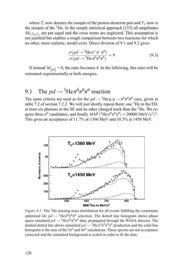
where Ti now denotes the isospin of the proton-deuteron pair and T f now isthe isospin of the 3He. In the simple statistical approach [153] all amplitudesMTiT3πT f are put equal and the cross terms are neglected. This assumption isnot justified but enables a rough comparison between two reactions for whichno other, more realistic, model exist. Direct division of 9.1 and 9.2 gives

σ(pd→ 3Heπ+π−π0)σ(pd→ 3Heπ0π0π0)

= 9 (9.3)

If instead M 12 0 1

2= 0, the ratio becomes 4. In the following, this ratio will be

estimated experimentally at both energies.

9.1 The pd→ 3Heπ0π0π0 reactionThe same criteria are used as for the pd→ 3Heη,η→ π0π0π0 case, given intable 7.2 of section 7.2.2. We will just shortly repeat them: one 3He in the FD,at least six photons in the SE and no other charged track than the 3He. We re-quire three π0 candidates, and finally MM2(3Heπ0π0π0) < 20000(MeV/c2)2.This gives an acceptance of 11.7% at 1360 MeV and 10.3% at 1450 MeV.

Figure 9.1: The 3He missing mass distribution for all events fulfilling the constraintsoptimised for pd → 3Heπ0π0π0 selection. The dotted line histogram shows phasespace simulated pd→ 3Heπ0π0π0 data, propagated through the WASA detector. Thedashed-dotted line shows simulated pd→ 3Heπ0π0π0π0 production and the solid linehistogram is the sum of the 3π0 and 4π0 simulations. These spectra are not acceptancecorrected and the simulated background is scaled in order to fit the data.

120

The 3He missing mass distributions at both energies for all events fulfill-ing the constraints are shown in figure 9.1. The dotted line shows simulatedpd→ 3Heπ0π0π0 data assuming phase space production. Simulated 3π0 datamatch the experimental data for low and medium missing masses (except atthe η peak, which is expected), but at high MM(3He), the matching betweendata and phase space Monte Carlo is poor. Why?

It is reasonable to assume a contribution in from pd → 3Heπ0π0π0π0,either from direct production or from production via ηπ0 inpd → 3Heηπ0,η→ π0π0π0π0. In these two reactions, eight photons areproduced.

The selection criteria optimised for 3π0 selection give an acceptance of 26%for 4π0 (same for direct production as for production via ηπ0) production at1360 MeV and 23% at 1450 MeV. This is more than twice as large as theacceptance for 3π0 production. The data obtained from phase space MonteCarlo simulations of pd→ 3Heπ0π0π0π0 are shown in the dashed-dotted linehistograms in the upper and lower panel of figure 9.1. Adding the contri-butions from 3π0 and 4π0 together (the fit is made by hand) gives the solidline histograms in figure 9.1. We obtain N4π0 = 250 at Tp = 1360 MeV andN4π0 = 800 at Tp = 1450 MeV, now giving N3π0 = 1400 and N3π0 = 4500at Tp = 1360 MeV and Tp = 1450 MeV, respectively. This corresponds to3π0 cross sections of 180 nb and 115 nb. The statistical uncertainty of N3π0

is given by σ2stat=Ntot=N3π0+Nη+N4π0 which becomes 3% (2%) at Tp=1360

MeV (Tp=1450 MeV). When we calculate the statistical uncertainty of N4π0 ,we instead take the square root of the number of events for which MM(3He)> 540 MeV/c2, since events at lower missing masses must come from othersources than pd→3 Heπ0π0π0π0. This gives a statistical uncertainty of 17%at 1360 MeV and 9% at 1450 MeV.

It is also possible that the 3π0 production mechanism is not dominatedby phase space production. However, in section 8.3 it was shown thatthe matching between experimental data and phase space Monte Carlopd→ 3Heπ+π−π0 is very good. Could the production mechanisms of π0π0π0

and π+π−π0 be very different from each other? Possibly, that depends on thematrix elements M 1

2 1 12

and M 12 0 1

2. Assuming that all events in the upper and

lower panel of figure 9.1 that do not originate from η→ π0π0π0 come fromdirect 3π0 production, we get N3π0 = 1650 at Tp = 1360 MeV and N3π0 =5300 at Tp = 1450 MeV which corresponds to cross sections of 212 nb and135 nb, respectively.

Since the mixture of 3π0 and 4π0 events reproduces the experimental dis-tributions very well, the 3π0 cross sections obtained assuming a contributionfrom 4π0 have been taken in favour of the latter ones. The difference betweenthe results with and without a 4π0 contribution is treated as a systematic un-certainty.

Furthermore, the pd →3He4π0 cross sections are estimated toσtot = 15 ± 3 nb at 1360 MeV and σtot = 9 ± 1 nb at 1450 MeV, where the

121

Table 9.1: The cross sections obtained using the sample of events fulfilling the se-lection criteria optimised for pd →3He3π0 selection. In addition to the systematicuncertainty given in the table, there is a normalisation uncertainty of 29% at 1360MeV and one of 12% at 1450 MeV.

Reaction Tp (MeV) σ (μb) stat. unc. (μb) syst. unc. (μb)pd→3He3π0 1360 0.180 ±0.006 +0.032pd→3He4π0 1360 0.015 ±0.003pd→3He3π0 1450 0.115 ±0.003 +0.020pd→3He4π0 1450 0.009 ±0.001

uncertainties are statistical only. The four π0 mesons can be produced eitherdirectly or through pd→3 Heηπ0, η→ 3π0. We will come back to how largethe contribution from ηπ0 is in section 10.

Background from reactions like quasi-free pp → ppπ0π0π0 witha proton misidentified as a 3He is expected to be neglible. The crosssection of pp→ ppπ0π0π0 is about an order of magnitide larger than thepd→3 Heπ0π0π0 at this energy [120, 147], but the probability that an eventfrom a reactions with p or d in the final state instead of 3He would survivethe constraints applied, is smaller than 0.001%.

The cross sections and their uncertainties are summarised in table 9.1.

9.2 The pd→ 3Heπ+π−π0 reactionFirst, events are selected according to the criteria given in 7.2.3, optimised forselection of pd→3Heω,ω→ π+π−π0 and pd→3Heη,η→ π+π−π0 and givenin table 7.3 and 8.1.

A short repetition:, one 3He, at least two photons in the SE and two or morehits in the PS are required. Two photons fulfill |IM(γγ)−mπ0 | < 45MeV/c2,the missing mass of the 3Heπ0-system must be larger than 250 MeV andthe total energy deposit in the SE must not exceed 900 MeV. As previouslystated, this gives a π+π−π0 acceptance of 35% at Tp = 1360 MeV and 31% atTp = 1450 MeV, assuming phase space production.

However, without reconstructing all final state particles, it is difficult toseparate “good” events in a continuum from unwanted background that forexample originate from overlapping events. When studying η’s and ω’s thatproblem does not arise since these mesons are identified by their peak in the3He missing mass distribution. Chance coincidences should be more evenlydistributed and quite easily separated from the events in the η and ω peaks.

If information from the MDC is used, stricter constraints can be applied andthe background from for example chance coincidences further reduced.

122

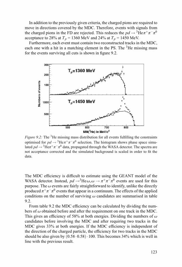
In addition to the previously given criteria, the charged pions are required tomove in directions covered by the MDC. Therefore, events with signals fromthe charged pions in the FD are rejected. This reduces the pd→ 3Heπ+π−π0

acceptance to 28% at Tp = 1360 MeV and 24% at Tp = 1450 MeV.Furthermore, each event must contain two reconstructed tracks in the MDC,

each one with a hit in a matching element in the PS. The 3He missing massfor the events surviving all cuts is shown in figure 9.2.

Figure 9.2: The 3He missing mass distribution for all events fulfilling the constraintsoptimised for pd→ 3Heπ+π−π0 selection. The histogram shows phase space simu-lated pd→ 3Heπ+π−π0 data, propagated through the WASA detector. The spectra arenot acceptance corrected and the simulated background is scaled in order to fit thedata.

The MDC efficiency is difficult to estimate using the GEANT model of theWASA detector. Instead, pd →3Heω,ω→ π+π−π0 events are used for thispurpose. The ω events are fairly straightforward to identify, unlike the directlyproduced π+π−π0 events that appear in a continuum. The effects of the appliedconditions on the number of surviving ω candidates are summarised in table9.2.

From table 9.2 the MDC efficiency can be calculated by dividing the num-bers of ω obtained before and after the requirement on one track in the MDC.This gives an efficiency of 58% at both energies. Dividing the numbers of ωcandidates before involving the MDC and after requiring two tracks in theMDC gives 33% at both energies. If the MDC efficiency is independent ofthe direction of the charged particle, the efficiency for two tracks in the MDCshould be also given by (0.58 ·0.58) ·100. This becomes 34% which is well inline with the previous result.

123

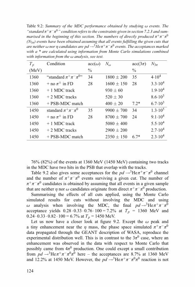
Table 9.2: Summary of the MDC performance obtained by studying ω events. The“standard π+π−π0” condition refers to the constraints given in section 7.2.3 and sum-marised in the beginning of this section. The numbers of directly produced π+π−π0

(N3π) events have been obtained assuming that all events fulfilling the given cuts thatare neither ω nor η candidates are pd→3Heπ+π−π0 events. The acceptances markedwith a * are calculated using information from Monte Carlo simulations combinedwith information from the ω analysis, see text.

Tp Condition acc(ω) Nω acc(3π) N3π

(MeV) % %1360 “standard π+π−π0” 34 1800 ± 200 35 4·104

1360 + no π± in FD 28 1600 ± 150 28 3.3·104

1360 + 1 MDC track 930 ± 60 1.9·104

1360 + 2 MDC tracks 520 ± 30 8.6·103

1360 + PSB-MDC match 400 ± 20 7.2* 6.7·103

1450 standard π+π−π0 35 9900 ± 700 34 1.3·105

1450 + no π± in FD 28 8700 ± 700 24 9.1·104

1450 + 1 MDC track 5080 ± 400 5.5·104

1450 + 2 MDC tracks 2900 ± 200 2.7·104

1450 + PSB-MDC match 2350 ± 150 6.7* 2.3·104

76% (82%) of the events at 1360 MeV (1450 MeV) containing two tracksin the MDC have two hits in the PSB that overlap with the tracks.

Table 9.2 also gives some acceptances for the pd →3Heπ+π−π0 channeland the number of π+π−π0 events surviving a given cut. The number ofπ+π−π0 candidates is obtained by assuming that all events in a given samplethat are neither η nor ω candidates originate from direct π+π−π0 production.

Summarising the effects of all cuts applied, using the Monte Carlosimulated results for cuts without involving the MDC and usingω analysis when involving the MDC, the final pd→3Heπ+π−π0

acceptance yields 0.28 ·0.33 ·0.76 ·100 = 7.2% at Tp = 1360 MeV and0.24 ·0.33 ·0.82 ·100 = 6.7% at Tp = 1450 MeV.

Let us now have a closer look at figure 9.2. Except the ω peak anda tiny enhancement near the η mass, the phase space simulated π+π−π0

data propagated through the GEANT description of WASA, reproduce theexperimental distribution well. This is in contrast to the 3π0 case, where anenhancement was observed in the data with respect to Monte Carlo thatpossibly came from 4π0 production. One could except a small contributionfrom pd →3Heπ+π−π0π0 here – the acceptances are 8.7% at 1360 MeVand 12.2% at 1450 MeV. However, the pd →3Heπ+π−π0π0 reaction is not

124

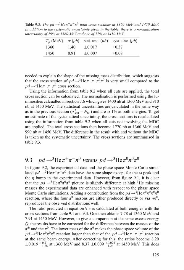
Table 9.3: The pd →3Heπ+π−π0 total cross sections at 1360 MeV and 1450 MeV.In addition to the systematic uncertainty given in the table, there is a normalisationuncertainty of 29% at 1360 MeV and one of 12% at 1450 MeV.

Tp (MeV) σ (μb) stat. unc. (μb) syst. unc. (μb)1360 1.40 ±0.017 +0.371450 0.91 ±0.007 +0.08

needed to explain the shape of the missing mass distribution, which suggeststhat the cross section of pd→3Heπ+π−π0π0 is very small compared to thepd→3Heπ+π−π0 cross section.

Using the information from table 9.2 when all cuts are applied, the totalcross section can be calculated. The normalisation is performed using the lu-minosities calcualted in section 7.6 which gives 1400 nb at 1360 MeV and 910nb at 1450 MeV. The statistical uncertainties are calculated in the same wayas in the previous section (σ2

stat = Ntot) and are ≈ 1% at both energies. To getan estimate of the systematical uncertainty, the cross sections is recalculatedusing the information from table 9.2 when all cuts not involving the MDCare applied. The total cross sections then become 1770 nb at 1360 MeV and990 nb at 1450 MeV. The difference in the result with and without the MDCis taken as the systematic uncertainty. The cross sections are summarised intable 9.3.

9.3 pd→3Heπ+π−π0 versus pd→3Heπ0π0π0

In figure 9.2, the experimental data and the phase space Monte Carlo simu-lated pd→3Heπ+π−π0 data have the same shape except for the ω peak andthe η bump in the experimental data. However, from figure 9.1, it is clearthat the pd →3Heπ0π0π0 picture is slightly different: at high 3He missingmasses the experimental data are enhanced with respect to the phase spaceMonte Carlo simulations. Adding a contribution from the pd→3Heπ0π0π0π0

reaction, where the four π0 mesons are either produced directly or via ηπ0,reproduces the observed distributions well.

The ratio predicted in equation 9.3 is calculated at both energies with thecross sections from table 9.1 and 9.3. One then obtains 7.78 at 1360 MeV and7.91 at 1450 MeV. However, to give a comparison at the same excess energyQ, the results have to be corrected for the difference between the masses of theπ± and the π0. The lower mass of the π0 makes the phase space volume of thepd→3Heπ0π0π0 reaction larger than that of the pd→3Heπ+π−π0 reactionat the same beam energy. After correcting for this, the ratios become 8.29±0.019 +0.21

−1.28 at 1360 MeV and 8.37 ±0.009 +0.074−1.24 at 1450 MeV. This does

125

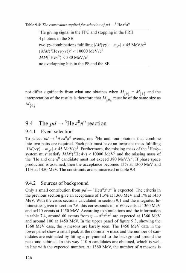
Table 9.4: The constraints applied for selection of pd→3 Heπ0π0

3He giving signal in the FPC and stopping in the FRH4 photons in the SEtwo γγ-combinations fulfilling |IM(γγ)−mπ0 | < 45 MeV/c2

(MM(3Heγγγγ))2 < 10000 MeV/c2

MM(3Heπ0) < 380 MeV/c2

no overlapping hits in the PS and the SE

not differ significatly from what one obtaines when M 12 0 1

2= M 1

2 1 12

and theinterpretation of the results is therefore that M 1

2 0 12

must be of the same size asM 1

2 0 12.

9.4 The pd→ 3Heπ0π0 reaction9.4.1 Event selectionTo select pd → 3Heπ0π0 events, one 3He and four photons that combineinto two pairs are required. Each pair must have an invariant mass fulfilling|IM(γγ)−mπ0 | < 45 MeV/c2. Furthermore, the missing mass of the 3He4γ-system must satisfy MM2(3He4γ) < 10000 MeV2 and the missing mass ofthe 3He and one π0 candidate must not exceed 380 MeV/c2. If phase spaceproduction is assumed, then the acceptance becomes 13% at 1360 MeV and11% at 1450 MeV. The constraints are summarised in table 9.4.

9.4.2 Sources of backgroundOnly a small contribution from pd→ 3Heπ0π0π0 is expected. The criteria inthe previous section give an acceptance of 1.3% at 1360 MeV and 1% at 1450MeV. With the cross sections calculated in section 9.1 and the integrated lu-minosities given in section 7.6, this corresponds to ≈160 events at 1360 MeVand ≈440 events at 1450 MeV. According to simulations and the informationin table 7.4, around 60 events from η→ π0π0π0 are expected at 1360 MeVand around 100 at 1450 MeV. In the upper panel of figure 9.3, showing the1360 MeV case, the η mesons are barely seen. The 1450 MeV data in thelower panel show a small peak at the nominal η mass and the number of can-didates are estimated by fitting a polynomial to the background around thepeak and subtract. In this way 110 η candidates are obtained, which is wellin line with the expected number. At 1360 MeV, the number of η mesons is

126

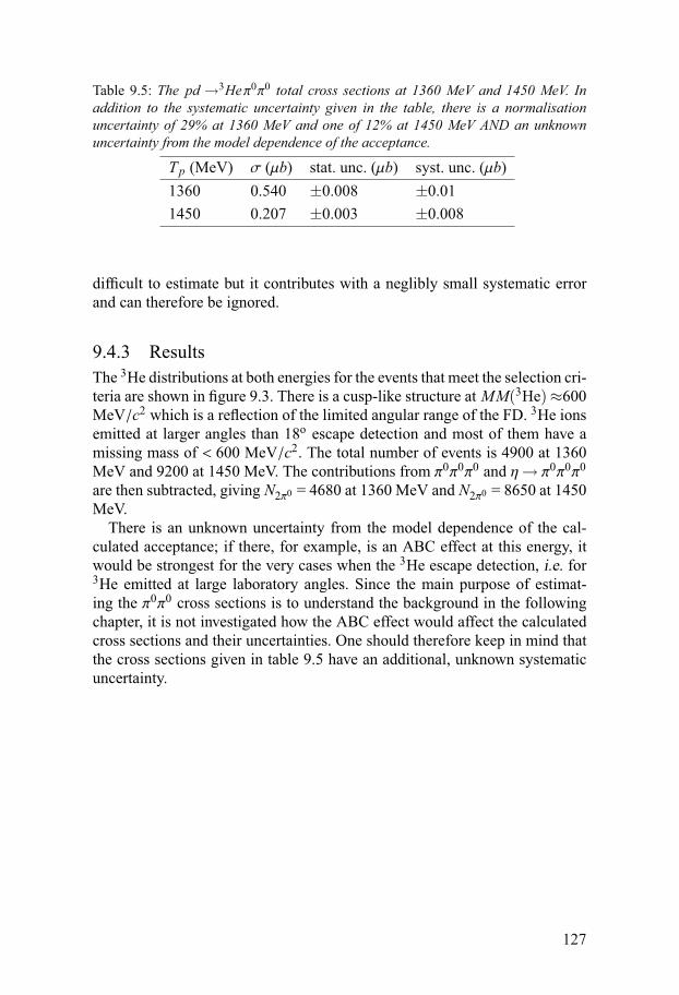
Table 9.5: The pd →3Heπ0π0 total cross sections at 1360 MeV and 1450 MeV. Inaddition to the systematic uncertainty given in the table, there is a normalisationuncertainty of 29% at 1360 MeV and one of 12% at 1450 MeV AND an unknownuncertainty from the model dependence of the acceptance.

Tp (MeV) σ (μb) stat. unc. (μb) syst. unc. (μb)1360 0.540 ±0.008 ±0.011450 0.207 ±0.003 ±0.008

difficult to estimate but it contributes with a neglibly small systematic errorand can therefore be ignored.

9.4.3 ResultsThe 3He distributions at both energies for the events that meet the selection cri-teria are shown in figure 9.3. There is a cusp-like structure at MM(3He)≈600MeV/c2 which is a reflection of the limited angular range of the FD. 3He ionsemitted at larger angles than 18o escape detection and most of them have amissing mass of < 600 MeV/c2. The total number of events is 4900 at 1360MeV and 9200 at 1450 MeV. The contributions from π0π0π0 and η→ π0π0π0

are then subtracted, giving N2π0 = 4680 at 1360 MeV and N2π0 = 8650 at 1450MeV.

There is an unknown uncertainty from the model dependence of the cal-culated acceptance; if there, for example, is an ABC effect at this energy, itwould be strongest for the very cases when the 3He escape detection, i.e. for3He emitted at large laboratory angles. Since the main purpose of estimat-ing the π0π0 cross sections is to understand the background in the followingchapter, it is not investigated how the ABC effect would affect the calculatedcross sections and their uncertainties. One should therefore keep in mind thatthe cross sections given in table 9.5 have an additional, unknown systematicuncertainty.

127

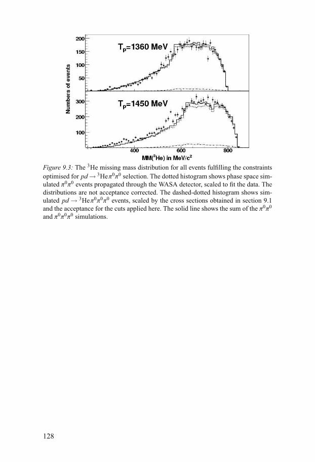
Figure 9.3: The 3He missing mass distribution for all events fulfilling the constraintsoptimised for pd→ 3Heπ0π0 selection. The dotted histogram shows phase space sim-ulated π0π0 events propagated through the WASA detector, scaled to fit the data. Thedistributions are not acceptance corrected. The dashed-dotted histogram shows sim-ulated pd→ 3Heπ0π0π0 events, scaled by the cross sections obtained in section 9.1and the acceptance for the cuts applied here. The solid line shows the sum of the π0π0

and π0π0π0 simulations.

128

10. The pd→ 3Heηπ0 reaction

Finally the pd→ 3Heηπ0 is studied. The analysis of this reaction was startedshortly before the submission of this thesis and a lot of work remains. Thenumerical values given in this chapter should therefore be considered as pre-liminary.

10.1 Event selectionThe pd→ 3Heηπ0 reaction was studied in the η→ γγ channel, which has abranching ratio of 39.4%. The cases when η decays into π0π0π0 (BR=32.5%)or π+π−π0 (BR=22.6%) have not been used in the search for the pd→ 3Heηπ0

events.At 1360 MeV, events with one 3He and four photons are selected.

Furthermore, one γγ combination must fulfill |IM(γγ)−mπ0 | < 45 MeV/c2.The two remaining photons must have an opening angle θηγγ larger than 80o

and an invariant mass that satisfies |IM(γγ)−mη| < 150 MeV/c2. Finally,MM2(3He4γ) < 10000 MeV2 must be fulfilled. These selection criteria givean acceptance of 10%. At 1450 MeV, the same cuts are applied with themodification that the opening angle of the two photons constituting the ηcandidate now must be larger than 70o instead. At this energy, the acceptanceamounts to 9.7%. All selection criteria are summarised in table 10.1.

Table 10.1: The constraints applied for selection of pd→3 Heηπ0

3He giving signal in the FPC and stopping in the FRH4 photons in the SEone γγ-combination fulfilling |IM(γγ)−mπ0 | < 45 MeV/c2

one γγ-combination fulfilling |IM(γγ)−mη| < 150 MeV/c2

1360 MeV: θηγγ > 80o

1450 MeV: θηγγ > 70o

(MM(3Heγγγγ))2 < 10000 MeV/c2

no overlapping hits in the PS and the SE

129

10.1.1 Remark: effect from chance coincidencesIn section 7.4 it was shown that 6-8% of the events contain particles fromother events that overlap in time. This requires some caution when an exactnumber of photons is required as a selection criterium. The normalisation wasperformed using events where a minimum number of photons, instead of anexact number, was required. Since exactly four photons are required for ηπ0

selection, there will be an additional contribution to the normalisation uncer-tainty due to chance coincidences. If the uncertainties are added quadratically,the total normalisation uncertainty at becomes 30% at 1360 MeV and 14% at1450 MeV.

10.2 Sources of backgroundThe most important background channels are multipion production:pd→ 3Heπ0π0 and pd→ 3Heπ0π0π0. The acceptance for 2π0 productionwhen the constraints described in the previous section are applied, becomes3.7% at 1360 MeV and 3.5% at 1450 MeV. Production of 3π0 gives anacceptance of 0.7% at 1360 MeV and 0.8% at 1450 MeV.

Production of 4π0 in pd → 3Heπ0π0π0π0 and pd → 3Heηπ0 contributesneglibly at both energies – the acceptance is less than 0.1%.

10.3 Results10.3.1 IdentificationPreviously, different reactions have been identified by studying the missingmass distribution of the 3He. In reactions with two particles in the final state,like pd→ 3Heη and pd→ 3Heω, the mesons are relatively easily identifiedsince the events appear in a peak at the nominal mass of the meson. In thecase of the multi-pion channels, the events could be selected in such a waythat most events in a given sample came from the reaction of interest andvery little from background channels. For example, in figure 9.3, where thepd→3 Heπ0π0 is studied, the backround from π0π0π0 and η→ π0π0π0 con-stitute altogether around 5% (7%) of the total event sample at 1360 MeV(1450 MeV). In the ηπ0 case the situation is somewhat different. First, thepd →3 Heηπ0 reaction has a three-body final state and therefore the signalwill not appear as a peak in the 3He missing mass distribution. Furthermore,the ηπ0 cross section is expected to be much lower than the cross section ofthe multi-pion background channels. The identification procedure is thereforeslightly differently this time.

The calibration of the CD is performed using π0 events and the calibrationis therefore optimised for photons coming from π0 decays. The invariant mass

130

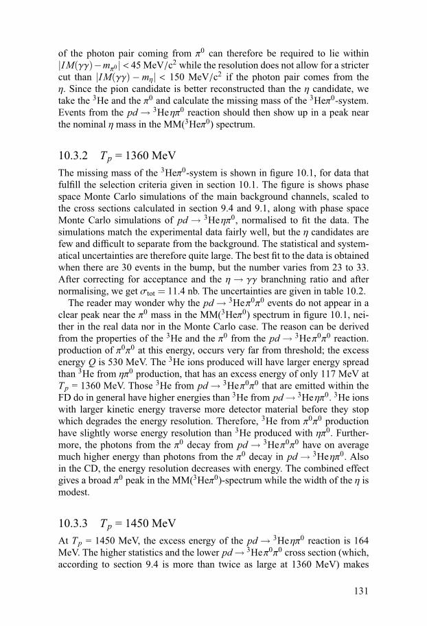
of the photon pair coming from π0 can therefore be required to lie within|IM(γγ)−mπ0 | < 45 MeV/c2 while the resolution does not allow for a strictercut than |IM(γγ)−mη| < 150 MeV/c2 if the photon pair comes from theη. Since the pion candidate is better reconstructed than the η candidate, wetake the 3He and the π0 and calculate the missing mass of the 3Heπ0-system.Events from the pd→ 3Heηπ0 reaction should then show up in a peak nearthe nominal η mass in the MM(3Heπ0) spectrum.

10.3.2 Tp = 1360 MeVThe missing mass of the 3Heπ0-system is shown in figure 10.1, for data thatfulfill the selection criteria given in section 10.1. The figure is shows phasespace Monte Carlo simulations of the main background channels, scaled tothe cross sections calculated in section 9.4 and 9.1, along with phase spaceMonte Carlo simulations of pd → 3Heηπ0, normalised to fit the data. Thesimulations match the experimental data fairly well, but the η candidates arefew and difficult to separate from the background. The statistical and system-atical uncertainties are therefore quite large. The best fit to the data is obtainedwhen there are 30 events in the bump, but the number varies from 23 to 33.After correcting for acceptance and the η→ γγ branchning ratio and afternormalising, we get σtot = 11.4 nb. The uncertainties are given in table 10.2.

The reader may wonder why the pd→ 3Heπ0π0 events do not appear in aclear peak near the π0 mass in the MM(3Heπ0) spectrum in figure 10.1, nei-ther in the real data nor in the Monte Carlo case. The reason can be derivedfrom the properties of the 3He and the π0 from the pd→ 3Heπ0π0 reaction.production of π0π0 at this energy, occurs very far from threshold; the excessenergy Q is 530 MeV. The 3He ions produced will have larger energy spreadthan 3He from ηπ0 production, that has an excess energy of only 117 MeV atTp = 1360 MeV. Those 3He from pd→ 3Heπ0π0 that are emitted within theFD do in general have higher energies than 3He from pd→ 3Heηπ0. 3He ionswith larger kinetic energy traverse more detector material before they stopwhich degrades the energy resolution. Therefore, 3He from π0π0 productionhave slightly worse energy resolution than 3He produced with ηπ0. Further-more, the photons from the π0 decay from pd→ 3Heπ0π0 have on averagemuch higher energy than photons from the π0 decay in pd→ 3Heηπ0. Alsoin the CD, the energy resolution decreases with energy. The combined effectgives a broad π0 peak in the MM(3Heπ0)-spectrum while the width of the η ismodest.

10.3.3 Tp = 1450 MeVAt Tp = 1450 MeV, the excess energy of the pd→ 3Heηπ0 reaction is 164MeV. The higher statistics and the lower pd→ 3Heπ0π0 cross section (which,according to section 9.4 is more than twice as large at 1360 MeV) makes

131

Figure 10.1: The missing mass of the 3Heπ0-system for 1360 MeV data fulfilling theconstraints given in the text. The dashed-dotted line shows Monte Carlo simulationsof pd→ 3Heπ0π0, scaled to the cross section given in section 9.4, while the dottedline shows simulated pd→ 3Heπ0π0π0 data scaled to the cross section given in sec-tion 9.1. The shaded histogram shows phase space Monte Carlo simulations of thepd→ 3Heηπ0 reaction and the black line is a sum of all Monte Carlo data. The datashown in this spectrum are not acceptance corrected.

Table 10.2: The pd→3Heηπ0 total cross sections at 1360 MeV and 1450 MeV. In ad-dition to the systematic uncertainties given in the table, there is a total normalisationuncertainty, including also the effect from chance coincidences, of 30% at 1360 MeVand one of 14% at 1450 MeV.

Tp (MeV) σ (μb) stat. unc. (μb) syst. unc. (μb)1360 0.0114 ±0.004 +0.0011

−0.00271450 0.0172 ±0.001 +0.0014

−0.0021

the identification easier. In figure 10.2, where the missing mass of the 3Heπ0-system is shown, there is indeed a peak around the nominal η mass, with awidth which is consistent with the results from the Monte Carlo simulations.The peak contains 250 +20

−30 events when the background is subtracted, whichcorresponds to a cross section of 17.2 nb. The cross sections and the uncer-tainties are summarised in table 10.2.

It should be noted that if |IM(γγ)−mη| < 100 MeV/c2 instead, the peakat the η mass in the MM(3Heπ0) spectrum has the same width as before. Thesignal-to-background ratio is somewhat improved which is also expected from

132

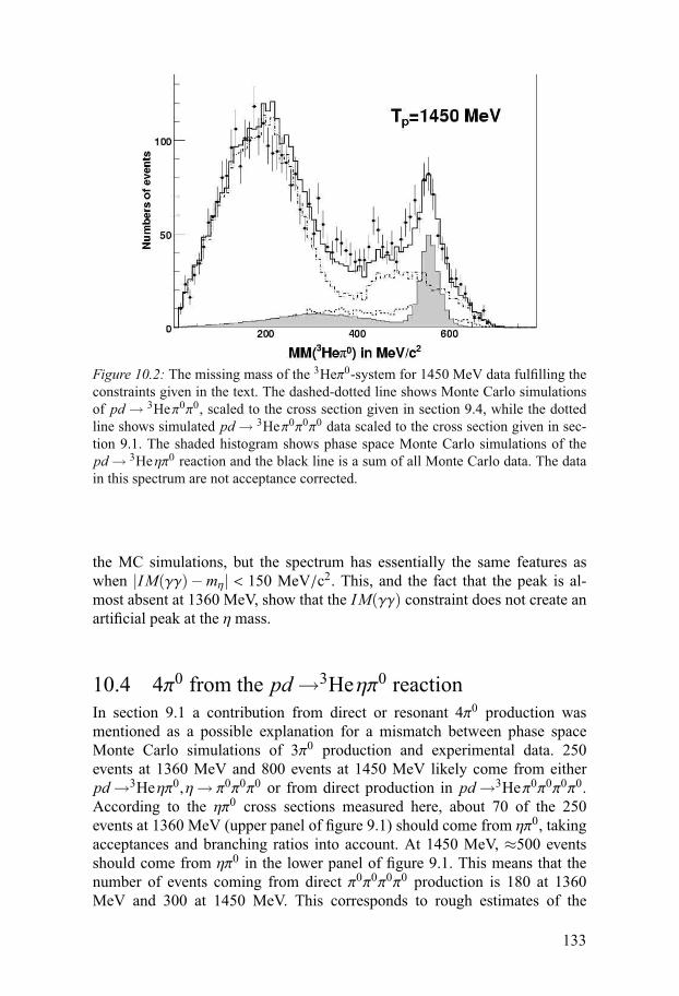
Figure 10.2: The missing mass of the 3Heπ0-system for 1450 MeV data fulfilling theconstraints given in the text. The dashed-dotted line shows Monte Carlo simulationsof pd→ 3Heπ0π0, scaled to the cross section given in section 9.4, while the dottedline shows simulated pd→ 3Heπ0π0π0 data scaled to the cross section given in sec-tion 9.1. The shaded histogram shows phase space Monte Carlo simulations of thepd→ 3Heηπ0 reaction and the black line is a sum of all Monte Carlo data. The datain this spectrum are not acceptance corrected.

the MC simulations, but the spectrum has essentially the same features aswhen |IM(γγ)−mη| < 150 MeV/c2. This, and the fact that the peak is al-most absent at 1360 MeV, show that the IM(γγ) constraint does not create anartificial peak at the η mass.

10.4 4π0 from the pd→3Heηπ0 reactionIn section 9.1 a contribution from direct or resonant 4π0 production wasmentioned as a possible explanation for a mismatch between phase spaceMonte Carlo simulations of 3π0 production and experimental data. 250events at 1360 MeV and 800 events at 1450 MeV likely come from eitherpd→3Heηπ0,η→ π0π0π0 or from direct production in pd→3Heπ0π0π0π0.According to the ηπ0 cross sections measured here, about 70 of the 250events at 1360 MeV (upper panel of figure 9.1) should come from ηπ0, takingacceptances and branching ratios into account. At 1450 MeV, ≈500 eventsshould come from ηπ0 in the lower panel of figure 9.1. This means that thenumber of events coming from direct π0π0π0π0 production is 180 at 1360MeV and 300 at 1450 MeV. This corresponds to rough estimates of the

133

pd→3Heπ0π0π0π0 cross sections of σtot = 10.4 ± 2.1 nb at 1360 MeV andσtot = 3.4 ± 0.3 nb at 1450 MeV.

134

11. Summary and discussion

Meson production in proton-deuteron collisions has been studied at two beamenergies – 1360 MeV and 1450 MeV – with the WASA detector facility. Inthis thesis, data from reactions with a 3He in the final state are analysed. Inthe following, I will summarise the most important findings that have emergedfrom this work.

11.1 The pd→3Heη reactionThe pd →3Heη reaction was studied at both energies and the threemost imortant decay channels of the η meson (η → γγ, η → π0π0π0 andη → π+π−π0) were compared. The η → γγ samples at both energiescontain very little background and were used for normalisation of thedata. The integrated luminosity times the trigger efficiency at 1360 MeVwas obtained to L ·εtrig = 66.6 nb−1 with an uncertainty of 29% while at1450 MeV it was estimated to L ·εtrig = 381.2 nb−1 with an uncertainty of12%. The difference between the acceptance and branching ratio correctednumber of events obtained from the different decay channels was within theuncertainties, showing that the effects of the applied selection criteria arewell understood. The angular distribution of the η meson was measured. Atboth energies, strong forward enhancements were observed. The total crosssection at 1360 MeV was estimated to σtot = 151.6±9.3±12.6 nb with anadditional uncertainty from normalisation of 29%. At 1450 MeV we obtainedσtot = 80.9±3.6±2.5 nb with a normalisation uncertainty of 12%.

11.2 The pd→3Heω reactionThe ω angular distributions from the pd→3Heω reaction were measured atboth energies and constitute the first measurements covering the whole angu-lar range. At 1360 MeV, the shape is consistent with isotropy whereas at 1450MeV, strong rises are observed at the extreme angles. Calculations performedby K.P. Khemchandani using a two-step model, predict a small forward en-hancement at 1360 MeV and a shape with suppressed differential cross sec-tions at extreme angles at 1450 MeV. Thus there is a striking disagreementbetween the shape obtained from theory and from experiment at 1450 MeV.

135

Why does the two-step model fail to describe the shape of the ω angulardistribution? In section 2.2, a study by Khemchandani is summarised wherethe source of the shape of the angular distribution is investigated. It was foundthat at large and small θ∗ω, the two-step model gives a poor velocity match-ing between the proton and the deuteron in the final step which suppressesthe probability of fusing into a 3He. This in turn suppresses the differentialcross section at these angles. Since the experimentally measured cross sectionshows strong rises in the very same angular regions, this suggests contribu-tions from other mechanism than that of the two-step model. A similar modelas the one used here was also used by Kondratyuk and Uzikov [83] when theycalculated the differential cross section dσ/dΩ∗ω at θ∗ω = 180o. It is possiblethat poor velocity matching at extreme angles caused their, by an order ofmagnitude, underprediction of the SPESIV data [64].

In this thesis, we were not able to test the rescattering hypothesis suggestedby Wurzinger in [64]. In order to bring clarity into this, a new, high statisticsmeasurement near threshold would be valuable. According to [64], rescatter-ing would affect the measured cross section at around 1380 MeV and below.The WASA data at 1360 MeV have too large statistical and systematical un-certainties to test the rescattering hypothesis.

An angular distribution of the ω, taken close to threshold with high statis-tics, would give welcome input to further studies of the production mecha-nism.

The total cross section at 1360 MeV was estimated toσtot = 84.6±4.0±4.8 nb with a normalisation uncertainty of 29%.At 1450 MeV the result was σtot = 83.6±1.5±2.2 nb. These are the firstmeasurements of the total cross section of the pd→3Heω reaction. Thetwo-step model underpredicts the data with an order of magnitude at 1360MeV and with a factor of two at 1450 MeV.

We have also studied the tensor polarisation of the ω. This was achievedby reconstructing the angular distributions of the decay pions. In particular,the distribution of the angle between the beam direction and the normal of theω→ π+π−π0 decay plane was studied. At 1450 MeV, we also measured theangle between the photon from the ω→ π0γ decay and the beam direction.The results were in good agreement and showed that the ω meson is producedunpolarised in the pd→3Heω reaction. This is in sharp contrast to a recentmeasurement of the φ polarisation in pd→3Heφ made by the MOMO collab-oration [107]. The MOMO measurement showed that the φmeson is producedalmost completely polarised. This raises the question whether the OZI rule isapplicable in this case – the difference in the production cross sections for ωand φ could be a consequence of differences in the production mechanismsand the nature of the meson-nucleon interaction rather than the difference inthe quark structure of the participating mesons and nucleons.

136

Beyond the scope of this thesis, it was also investigated whether events fromthe pd→ pdω reaction could be found. However, since this was done after theruns when the data were collected, no special trigger had been developed andused for the purpose. The minimum bias triggers that were used during theruns were prescaled with high factors and did therefore not collect a sufficientamount of data with pd candidates in the final state. Furthermore, the calibra-tion must be even better in order to separate protons from deuterons properly.The excellent statistics that is needed for high quality calibration should bepossible to achieve with WASA at COSY. A measurement of the pd→ pdωreaction has not been measured before and it could give further clues aboutthe ω production mechanism.

11.3 Multipion productionMultipion production constitutes the main background of pd →3Heη,pd→3Heω and pd→3Heηπ0. Knowing the cross sections of pd→3Heπ0π0,pd →3Heπ0π0π0 and pd →3Heπ+π−π0 is very helpful in the analysis ofother reactions but they are also interesting in their own right. In particular, acalculation of isospin amplitude within the statistical model predicts the ratiobetween σtot(π+π−π0) and σtot(π0π0π0) to be 9. Our measurements givea ratio of 8.29 ±0.019 +0.21

−1.28 at 1360 MeV and 8.37 ±0.009 +0.074−1.24 at 1450

MeV, which do not differ significantly from the statistical model in whichM 1

2 0 12

= M 12 1 1

2. This can be interpreted as if the isospin amplitudes M 1

2 0 12

andM 1

2 1 12

are of the same size.The pd →3Heπ0π0π0 cross section was determined to

σtot = 180±6+32 nb at 1360 MeV with a normalisation uncer-tainty of 29%. At 1450 MeV, one obtains σtot = 115±3+20 nb with anadditional uncertainty from normalisation of 12%. Rough estimates of the4π0 cross section were obtained to σtot ≈ 15 nb at 1360 MeV and σtot ≈ 9 nbat 1450 MeV, where the four pions can be produced either directly ortrough pd→3Heηπ0,η→ 3π0. After studying the pd→3Heηπ0, roughestimates of the cross section for direct 4π0 production were obtained toσtot = 10.4 ± 2.1 nb at 1360 MeV and σtot = 3.4 ± 0.3 nb at 1450 MeV,where the uncertainties are statistical only.pd→3Heπ+π−π0 cross section was found to be σtot = 1400±17+370 nb

at 1360 MeV and σtot = 910±7+80 nb at 1450 MeV, with additional nor-malisation uncertainties of 29% and 12%, respectively.

137

11.4 The pd→3Heηπ0 reactionThe study of the pd→3Heηπ0 reaction started shortly before this thesis wassubmitted and the analysis is not finished yet.

The total cross section was measured at both energies. At 1360 MeV, thestatistical and systematical uncertainties are large and the cross section mea-surement is based on about 30 events, which corresponds to a cross section ofσtot = 11.4 ± 4.0 +1.1

−2.7 nb with an additional uncertainty from normalisation of30%.

At 1450 MeV, the statistics is better and the the signal-to-background ratiois larger. The cross section was estimated to σtot = 17.2 ± 1.0 +1.4

−2.1 nb with anormalisation uncertainty of 14%.

The next step is to extract the invariant mass of the ηπ0-system. The shapemay give information about the production mechanism – for example, an en-hancement with respect to phase space simulations at high IM(ηπ0) may in-dicate production via the tail of the a0(980) resonance. Studying this distribu-tion will only be possible at 1450 MeV because the statistics is insufficient at1360 MeV. In order to obtain reliable distributions of the final state particles,it has to be found out how to treat the multipion background in a proper way.

138

12. Summary in Swedish:Mesonproduktion i pd-kollisioner

Jag kommer att börja med att försöka förklara vad hadronfysik är, på ett sättsom förhoppningsvis även icke-fysiker kan förstå. Nivån höjs undan för undanalltmedan jag går djupare in i hadronfysikens värld och slutligen presenterarmin egen forsknings roll i den.

12.1 Vad är hadronfysik?Inom hadronfysik studerar man den så kallade starka kraften. Den utgör enav de fyra fundamentala krafterna som finns: gravitationskraften, den elektro-magnetiska kraften, den svaga kraften och den starka kraften.

Gravitationen verkar mellan alla föremål som har massa, eller mer generelltenergi. Massa och energi kopplas nämligen samman enligt Einsteins berömdaformel E = mc2. Gravitationen är den kraft som människan märker mest ivardagen – till exempel håller den oss kvar på jorden – men mellan partik-lar med mycket liten massa, är den tämligen obetydlig jämfört med de andrakrafterna. Inom hadronfysiken bortser man från den helt.

Den elektromagnetiska kraften verkar mellan elektriskt laddade föremål.På mikronivå växelverkar två laddade partiklar, t.ex. två elektroner, genom attskicka en foton mellan sig. En foton är nämligen inte bara en “ljuspartikel”,den är också förmedlare av den elektomagnetiska kraften. Hur går då dettatill? För att illustrera tar vi ett exempel med person A och person B som sitter ivarsin båt på en sjö. A har en boll som hon kastar till B. När A kastar, kommerA:s båt att röra sig en aning i motsatt riktning jämfört med bollens. När Bfångar bollen, kommer hennes båt röra sig en aning i den riktning bollen kom.Utan att A och B har rört vid varandras båtar, har A och B växelverkat så attderas båtar rört sig från varandra. Bollen har agerat kraftförmedlare i dettafall.

Precis som utbytet av bollen får båtarna att röra sig åt var sitt håll, får ettutbyte av en foton två elektroner att röra sig från varandra. Två partiklar medmotsatt laddning, till exempel en elektron och dess antipartikel positronen,dras mot varandra istället, och då fungerar inte liknelsen med bollen längre.Istället kan man, även om denna liknelse är något grovt tillyxad, föreställa sigatt A har en boomerang som hon kastar i riktning från B och som sedan rörsig i en båge i 360o så att den når B när den rör sig i riktningen mot A.

139

Den starka kraften verkar mellan partiklar med en annan slags laddningän den elektriska: så kallad färgladdning. Kvarkar är ett exempel på partiklarmed färgladdning. Enligt den s.k. standardmodellen finns det sex olika typerav kvarkar: u (upp), d (ner), s (sär), c (charm), b (botten), och t (topp). Dessaväxelverkar genom utbyte av gluoner. Hittills har vi kunnat dra paralleller tillhur elektromagnetismen fungerar, men här upphör likheterna. Ty medan denelektromagnetiska kraftförmedlaren, fotonen, är elektriskt neutral, och alltsåinte växelverkar med andra fotoner, bär gluonen själv färgladdning. Det be-tyder att gluoner kan växelverka med andra gluoner. Detta leder till att julängre bort från en färgladdning vi tar en annan färgladdning, desto starkareblir kraften emellan dem. Till slut blir kraften så stark att det “kostar” mer en-ergi att separera de två färgladdningarna ännu mer, än det “kostar” att bilda tvånya, motsatta, färgladdningar. Detta betyder att vi inte kan observera fria, isol-erade färgladdningar. Kvarkar uppträder därför aldrig ensamma, utan antingeni par tillsammans med en antikvark, så att parets totala färgladdning blir noll,eller i en triplett av kvarkar – baryoner – som också kan bilda ett färgneutraltobjekt. Det är därför man valt ordet “färg” för att beskriva den starka laddnin-gen: grönt, rött och blått ljus bildar tillsammans vitt (färglöst) ljus. Protonenär en triplett av två uppkvarkar och en nerkvark (se till vänster i figur 12.1),medan neutronen är en triplett av två nerkvarkar och en uppkvark.

Denna avhandling handlar om mesoner. De består av kvark-antikvark-par.Kvarkar brukar betecknas med q (där q kan bytas mot aktuell kvarktyp) ochantikvarkar med q. Till exempel består den lättaste mesonen π antingen av ud(π+, se till höger i figur 12.1) eller du (π−) eller av en uu-komponent och endd-komponent (π0).

Figure 12.1: Till vänster en proton, bestående av två uppkvarkar och en nerkvark, hårtsammanbundna med gluoner. Till höger mesonen π+, som består av en uppkvark ochen anti-nerkvark.

140

Den starka kraften verkar på mycket korta avstånd – inuti en proton tillexempel. Hur den starka kraften mellan kvarkarna inuti en proton fungerarförstår man numera ganska väl, genom läran om kvantkromdynamik.Avstånden mellan kvarkarna i en proton är korta; så korta att den starkakopplingskonstanten där är relativt “svag”. Kvarkarna uppträder som friapartiklar på dessa korta avstånd. Det gör beräkningarna enklare och deförutsägelser som görs stämmer väl överens med vad man mätt i experiment.På större avstånd blir det svårare ju större den starka kopplingskonsten blir.Riktigt svårt att tillämpa det man vet om kvarkar och gluoner blir det om manska titta på kraften mellan två protoner. Två protoner kan växelverka medvarandra genom den starka växelverkan trots att de är färgneutrala, eftersomderas beståndsdelar bär färgladdning. På samma sätt kan två elektrisktneutralt laddade atomer eller molekyler växelverka elektromagnetiskt medvarandra, genom s.k. van der Waals-kraft. Detta sker genom att atomernautbyter elektroner sinsemellan. Protonerna som växelverkar med varandragör det genom utbyte av mesoner, som hela tiden skapas och förintas inutiprotonerna. Så, istället för att vi beskriver växelverkan genom att kvarkarutbyter gluoner, beskriver vi den genom att baryoner utbyter mesonermed varandra. Detta kallas för en effektiv fältteori och kan härledas frånkvantkromdynamiken genom att baryoner och mesoner består av kvarkar,som är de fundamentala beståndsdelarna inom kvantkromdynamiken.Mesonerna som bildas och förintas inuti en baryon har en begränsadlivslängd. Enligt Heisenbergs osäkerhetsrelation får de bara existera underen tid som är omvänt proportionell mot mesonens massa. En lätt meson fårexistera längre tid än en tung meson och hinner alltså färdas en längre sträcka.Utbyte av lätta mesoner ger därmed växelverkan på längre avstånd än utbyteav tunga mesoner. Vidare ser växelverkan olika ut beroende på mesonensövriga egenskaper, till exempel dess spinn. Spinn kan förenklat beskrivas somatt en partikel snurrar kring sin egen axel, ett inre rörelsemängdsmoment. Föratt vi ska kunna förstå hur baryoner, som protoner och neutroner, växelverkarmed varandra, är det alltså helt avgörande att vi känner till mesonernasegenskaper i detalj. Detta är vad denna avhandling handlar om.

12.2 Hur studerar vi hadronfysik?Hur kan man då utföra experiment på något som är så litet? Principen kan fak-tiskt, förenklat, beskrivas som en helt vanlig solig dag, då person C står ochtittar på en hund. Solen lyser på hunden, d.v.s. hunden träffas av fotoner, somstudsar på hunden. En del av de fotoner som studsar bort från hunden träf-far C:s ögon. I ögat startar en process som leder till att nervsignaler skickastill C:s hjärna. C tänker: “Hund!” Vad gör då C om hon vill se något som ärmycket mindre än hunden? Som ni kanske vet kan ljus beskrivas både sompartiklar (fotoner) och som (elektromagnetiska) vågor. Det ljus våra ögon kan

141

uppfatta är vågor med våglängder mellan ca 400 nm (1 nm = 0.000000001 m)och 700 nm. Vill vi “se” mycket mindre föremål än dem vi ser med blotta ögat,behöver vi kortare våglängder på det som “studsar” mot föremålet vi vill se.Fotoner med så korta våglängder som behövs för att se hur en atomkärna ser utinuti är inte överkomliga, men precis som vågor kan vara partiklar samtidigt,kan partiklar, såsom elektroner och protoner, beskrivas som vågor med en vissvåglängd. Vad man gör är att man accelererar till exempel elektroner eller pro-toner till hastigheter nära ljusets. Detta görs med hjälp av elektromagnetiskafält i en accelerator. Acceleratorn har i experimentalpartikelfysiken den rollsolen har i exemplet med C och hunden. Elektronerna eller protonerna, sam-lade i en stråle, får sedan, i denna höga hastighet kollidera med ett strålmål.Ett strålmål kan vara en gas, en vätska eller ett fast ämne och motsvaras i hun-dexemplet av själva hunden. Ibland låter man två accelerade partikelstrålarfrontalkrocka med varandra istället; exakt vilken metod som väljs beror påvad man vill undersöka med sitt experiment. Då partikelstrålarna krockar medvarandra, eller då en stråle krockar med ett strålmål, bildas vanligen nya par-tiklar av olika slag. Även dessa nya partiklar har i allmänhet en hög hastighet.Dessa partiklar detekteras i en detektor. Detektorn motsvaras av C:s öga i ex-emplet med C och hunden. Genom att signalerna i detektorn digitaliseras, kande nybildade partiklarnas massor, hastigheter och banor rekonstrueras medhjälp av datorprogram. Jämförelsen mellan hundexemplet och ett partikelex-periment illustreras i figur 12.2.

Med hjälp av datorer kan man också analysera vad det betyder fysikalisktatt just dessa partiklar bildats på just detta sätt med just dessa egenskaper, ochpå så sätt får man ökade kunskaper om materiens beståndsdelar och hur deväxelverkar. Datorerna i ett partikelfysikexperiment motsvaras av C:s hjärna ihundexemplet.

12.3 Mesonproduktion in pd-kollisionerI denna avhandling har mesonerna π,η och ω studerats. De data som analyser-ats kommer från The Svedberglaboratoriet i Uppsala. Där accellererades pro-toner (p) i den 82 meter långa CELSIUS-ringen där de fick krocka med pelletsav fruset deuterium (d), dvs. “tungt väte”, ett bundet tillstånd mellan en protonoch en neutron. I dessa krockar bildades heliumjoner och mesoner. De tungamesonerna, som η och ω, sönderföll i det närmaste omedelbart till pioner ellerfotoner. De neutrala pionerna sönderföll i sin tur direkt till fotoner. Fotonerna,heliumjonerna och de laddade pionerna mättes med WASA-detektorn.

Fokus har legat på ω-produktion. Jag har studerat hur stor sannolikhet detär att just den mesonen bildas vid olika energier, eller hastigheter, hos dekolliderande partiklarna. Jag har även undersökt i vilka riktningar de bildademesonerna beger sig. Resultaten har jämförts med beräkningar utifrån en teo-retisk modell. I denna modell bildas mesonen i en process som är uppdelad i

142

Figure 12.2: En analogi mellan en vardaglig situation där en person ser på enhund, och ett partikelfysikexperiment där en accellerator accellererar partiklar tillhastigheter nära ljusets, innan de krockas mot andra partiklar i ett stråmål. I krockenbildas nya partiklar, och genom att studera dessa får vi redan på hur materiens inre serut och fungerar.

flera steg. Överensstämmelsen mellan teori och experiment är inte särskilt godvilket betyder att de teoretiska modellerna behöver förbättras; det finns alltsåmer att lära.

Genom att mäta de π-mesoner (pioner) som ω sönderfaller till, får maninformation om polarisationen, dvs åt vilket håll ω-mesonen snurrar i förhål-lande till dels sin egen rörelseriktning, dels riktningen på protonen som deltari krocken. Vi upptäckte att ω-mesonen produceras helt opolariserad, vilket ärsärskilt intressant med tanke på att nya mätningar påω-mesonens “syster”,1 φ-mesonen, visar att den är nästan helt polariserad när den bildas i motsvarandereaktion. ω och φ skiljer sig bara åt när det gäller kvarkinnehållet (ω består aven uu-komponent, en dd-komponent och en liten ss-komponent medan φ tillstörsta delen består av en ss-komponent), men detta borde inte avgöra gradenav polarisation. Vår tolkning är istället att i proton-deuteron-kollisioner vidlåga och medelhöga energier, spelar meson-nukleon-växelverkan större rollän kvarkstrukturen.

1eller snarare SU(3)-partner, men det behöver vi inte gå in på här

143

Acknowledgement

This WASA trip lasted a lot longer than the original one, the one that tookplace in Stockholm, August 10, 1628, and at least for me, it had a happierending. Along the journey there have been happy moments and exciting eventsbut also tough periods. Tough those days when all work did not seem to payoff, and tough that day when we lost a good friend.There have been times when I thought I would never come to this point, writ-ing the last pages of a finished thesis. But now I am here, and that is thanks toa number of people that have supported me and helped me over the years.

First of all, I’d like to thank my supervisor Bo Höistad. You have always en-couraged me and convinced me that “things will work out”. You have let mego my own way but you have also given me good advice when I needed it.Besides, I appreciate that you participated in the shifts during “the last daysof CELSIUS”!Next in line to receive my gratitude is my other supervisor, Jozef Złomanczuk.Through the years, I have approached you with a countless number of ques-tions, and you always teach me something new. Furthermore, you never lookannoyed but just happy to help. Beer for you!Tord Johansson, thank you for good advice and interesting discussions duringmy time as a Ph.D. student. Your support during the release of “Maskros-fysiker” was also highly appreciated.I am also very grateful to my good friend Agnes Lundborg. I could not havehad a better office mate; our discussions about physics or gender or anythingelse always made me a little wiser. Even more importantly, sharing office withyou made work fun! “Maskrosfysiker” was an adventure that I learned a lotfrom.Kanchan P. Khemchandani, thank you for all interesting physics discussionsand for being a great theory teacher and a good friend. Colin Wilkin deservesa toast for convincing me about the potential of studying ω production, andfor help and advice over these yearsI also want to praise my comrade-in-pain, Henrik Petrén, for a countless num-ber of root/LaTeX/linux tips and for friendship and support.Pia Thörngren-Engblom and Emma Olsson, thank you for being friends andinofficial mentors for me during my Ph. D. studies.There have been and still are several WASA Ph. D. students with whom Ihave shared joy and pain these years: Samson Keleta, Marek Jacewicz, Inken

145

Koch, Filippo Capellaro, Levent Demirörs, Christian “Williams” Pauly,Michail Bashkanov, Tatiana Skorodko, Olena Khakimova, Florian Kren,Anette Pricking, Patrik Adlarsson.David Duniec, I miss you.The rest of the Uppsala WASA group has given me a lot of valuable inputthese years. Thank you Andrzej Kupsc, Hans Calén, Kjell Fransson, MagnusWolke and Pawel Marciniewski.A toast also for the TSL personnel in general and Carl-Johan Fridén andVolker Ziemann in particular, for all help during the WASA runs.The system administrators Ib Koersner and Teresa Kupsc have helped methrough many crises. What would I do without you two?I highly appreciate the input I have got from my proof-readers: Jozef Zło-manczuk, Bo Höistad, Agnes Lundborg, Magnus Wolke, Andrzej Kupsc, Kan-chan P. Khemchandani and Sandra Eriksson. Your comments have improvedthe thesis tremendously. Thanks also to David Eriksson for useful tips duringwriting this thesis.The other members of Ib-Karinz make this place rock! Tord “The Boss” Jo-hansson, Ane “Plätten” Håkansson, Fredrik Robelius, Christofer Willman,Ib “Salsa” Koersner, Henrik Petrén, Kristofer Jakobsson, Karin “Honkan”Holmqvist, Johan Alwall and my sister Eva Schönning.Over these years, many people have lightened up my lunches and cofféebreaks, not to mention the Thursday beers. In particular. I would like to thankHenrik Jäderström for being there during a difficult time. Others that havecontributed to the friendly environment here are Sheep-tipping Sophie, Erik,Elias, Magnus J, Camille, Oscar, Bjarte, P-A, Muffins-Micke, Peder, Arnaud,Bengt S, Bengt K, Martin, Carl-Oskar, Emma, Anna, Cajsa, Pawel P, Mat-tias E, Johan A, Johan R, Richard, Rikard, Örjan, Robban, Willman, Staffan,Anni, Tobbe, Joa, Magdalena, Frida, Mattias L, Pernilla, Lotta, Karen, KarinSt, Henrik S, Markus, Martino, Olle,Johan L, Mårten, Corinna...Inger Ericsson and Annika Elm, thank you for keeping this place going.Thanks to Anneli Andersson for your supervision during “Maskrosfysiker”and thanks to Annika Lindé for your support when it was published.Lots of hugs to all my friends. In particular I would like to mention Sandra,Helena and Elin L, for all nice lunches together during my Ph. D. studies,Emma J and Sofia Z for making my undergraduate studies so fun, Jane forcheering me up at work with emails and Anders, Jez, Jenny P and Karin K forbeing my “oldest” friends.My champagne-and-sauna-friends, Sanna, Elin E, Kristina, Sofi, Frida O andYwe for giving me my social life back after Ivar’s birth: cheerio!I also want to mention Smålandskören which has been an important part of mylife ever since 1997. In particular I want to thank Jennie for being the spiritand the driving force for so many years.The discussions within the “ESC-club”, with for example Linus and Camilla,make every Eurovision Song Contest final a long-lasting adventure.

146

My dear family: first of all I should mention that my mother’s resistanceagainst nuclear power what was made me interested in nuclear physics longago! But I am grateful to both my parents for making me interested in thepeople and the world around me. Hugs and kisses for Magnus, Eva, Erik andMax for all the memories we share. Also thanks to the “extended family”, youknow who you are.

Oscar, my better half: thank you for always being there for me, for taking meback to reality when I lose perspective and for laughing at the same things asme.

Ivar, every day at work I look forward to come home to your smiling face andyour hugs. Because of you, the past year has been the best ever. Jag är så gladatt jag har dig, min underbara pojke!

147

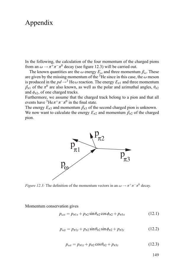
Appendix

In the following, the calculation of the four momentum of the charged pionsfrom an ω→ π+π−π0 decay (see figure 12.3) will be carried out.

The known quantities are the ω energy Eω and three momentum �pω. Theseare given by the missing momentum of the 3He since in this case, the ωmesonis produced in the pd→3 Heω reaction. The energy Eπ1 and three momentum�pπ1 of the π0 are also known, as well as the polar and azimuthal angles, θπ2and φπ2, of one charged tracks.Furthermore, we assume that the charged track belong to a pion and that allevents have 3Heπ+π−π0 in the final state.The energy Eπ3 and momentum �pπ3 of the second charged pion is unknown.We now want to calculate the energy Eπ2 and momentum �pπ2 of the chargedpion.

p

pp

pω

π1

π2

π3

Figure 12.3: The definition of the momentum vectors in an ω→ π+π−π0 decay.

Momentum conservation gives

pωx = pπ1x+ pπ2 sinθπ2 cosφπ2 + pπ3x (12.1)

pωy = pπ1y+ pπ2 sinθπ2 sinφπ2 + pπ3y (12.2)

pωz = pπ1z+ pπ2 cosθπ2 + pπ3z (12.3)

149

Then the unknown vector �pπ3 can be expressed in terms of the known quanti-ties and the unknown pπ2 =

√p2π2x+ p2

π2y+ p2π2z as follows:

pπ3x = A− pπ2 ·D (12.4)

pπ3y = B− pπ2 ·F (12.5)

pπ3z =C− pπ2 ·G (12.6)

where A, B, C, D, F and G are known and given by

A= pωx− pπ1x (12.7)

B= pωy− pπ1y (12.8)

C = pωz− pπ1z (12.9)

D= sinθπ2 cosφπ2 (12.10)

F = sinθπ2 sinφπ2 (12.11)

G = cosθπ2 (12.12)

Energy conservation gives

Eω = Eπ1 +Eπ2 +Eπ3 = Eπ1 +√p2π2 +m2

π2 +√p2π3 +m2

π3 (12.13)

Inserting 12.4-12.6 into 12.13 and using mπ2 = mπ3 = mπ+ = mπ− = mπ andsome algebra yields

2(Eω−Eπ1)√p2π2 +m2

π = (Eω−Eπ1)2−(A2+B2+C2)+2pπ2(AD+BF+CG)(12.14)

By definingα= (Eω−Eπ1)2− (A2 +B2 +C2) (12.15)

β= (AD+BF+CG) (12.16)

150

equation 12.14 can be simplified:

2(Eω−Eπ1)√p2π2 +m2

π = α+2βpπ2 (12.17)

We have thus arrived with one equation from which the unknown quantityp2π2, can be calculated. Knowing p2

π2, the energy and direction of both chargedpions can be obtained.

151

Bibliography

[1] H. Yukawa, Proc. Phys. Math. Soc. Japan 17 (1935) 48

[2] G. P. S. Occhialini and C. F. Powell, Nature 159 (1947) 186

[3] Prog. Theor. Phys. Supplement 3 (1956)

[4] A. Proca, J. Phys. Radium 7 (1936) 347

[5] N. Kemmer, Proc. Roy. Soc. A 166 (1938) 127

[6] G. Wick, Nature 142 (1938) 993

[7] M. Taketani, S. Nakamura and M. Sasaki, Prog. Theor. Phys. 4 (1951) 581

[8] P. Cziffra, M. H. MacGregor, M. J. Moravsik and H. P. Stapp, Phys. Rev. 114(1959) 880

[9] G. Breit, M. H. Hull, K. E. Lassila and K. D. Pyatt, Phys. Rev. 120 (1960) 2227

[10] G. Breit, Rev. Mod. Phys. 34 (1962) 766

[11] J. Iwadare, S. Otsuki, R. Tamagaki and W. Watari, Prog. Theor. Phys. 15 (1956)86

[12] J. Iwadare, S. Otsuki, R. Tamagaki and W. Watari, Prog. Theor. Phys. 16 (1956)455

[13] D. Y. Wong, Phys. Rev. Lett. 2 (1959) 406

[14] N. K. Glendenning and G. Kramer, Phys. Rev. 126 (1962) 2159

[15] M. Taketani, S. Machida, and S. Onuma Prog. Theor. Phys. 7 (1952) 45

[16] K. A. Brueckner and K. M. Watson, Phys. Rev. 90 (1953) 699; ibid. 92 (1953)1023

[17] R. J. N. Phillips, Rep. Prog. Phys. 22 (1959) 562

[18] M.J. Moravsik, The Two-Nucleon Interaction, Clarendon Press, Oxford (1963)

[19] A.R. Erwin et al., Phys. Rev. Lett. 6 (1961) 628

[20] B.C. Maglic et al., Phys. Rev. Lett. 7 (1961) 178

[21] A. Pevsner et al., Phys. Rev. Lett. 7 (1961) 421

153

[22] S. Ogawa et al., Prog. Theor. Phys. 39 (1967)

[23] R.A. Bryan and B.L. Scott, Phys. Rev. 177 (1969) 1435

[24] M.M. Nagels, T.A. Rijken and J.J. de Swart, Phys. Rev. D 17 (1978) 768

[25] V. G. J. Stoks et al., Phys. Rev. C 49 (1994) 2950

[26] R. Machleidt, Phys. Rev. C 63 (2001) 024001

[27] Y. Nambu and G. Jona-Lasinio, Phys. Rev. 122 (1961) 345; ibid. 124 (1961)246

[28] R. Vinh Mau, Mesons in Nuclei, Vol. 1, ed. by M. Rho and D. H. WilkinsonNorth-Holland, Amsterdam (1979) 151

[29] M. Lacombe et al., Phys. Rev. C 21 (1980) 861

[30] R. Machleidt, Adv. Nucl. Phys. 19 (1989) 189

[31] R. Machleidt, K. Holinde and C. Elstev, Phys. Rep. 149 (1987) 1

[32] M. Gell-Mann, California Institute of Technology Synchrotron Laboratory Re-port CTSL-20 (1961)

[33] M. Gell-Mann, Phys. Rev. 125 (1962) 1067

[34] Y. Ne’eman, Nucl. Phys. 26 (1962) 222

[35] M. Gell-Mann, Phys. Lett. 8 (1964) 214

[36] D. J. Gross, F. Wilczek, Phys. Rev. Lett. 30 (1973) 1343

[37] H. D. Politzer, Phys. Rev. Lett. 30 (1973) 1346

[38] F. Myhrer and J. Wroldsen, Rev. Mod. Phys. 60 (1988) 629

[39] T.A DeGrand, R.L. Jaffe, K. Johnson and J.E. Kiskis, Phys. Rev. D 12 (1975)2060

[40] G.E. Brown and M. Rho, Phys. Lett. B 82 (1979) 177

[41] G.E. Brown, M. Rho and V. Vento, Phys. Lett. B 84 (1979) 383

[42] A.W. Thomas, S. Théberge and G.A. Miller, Phys. Rev. D 24 (1981) 216

[43] A.W. Thomas, Adv. Nucl. Phys. 13 (1983) 1

[44] N.K. Pak and H.C. Tze, Annals Phys. 117 (1979) 164

[45] E. Witten, Nucl. Phys. B 160 (1979) 57

[46] J.M. Gipson and H.C. Tze, Nucl. Phys. B 183 (1981) 524

154

[47] T. H. R. Skyrme, Proc. Roy. Soc. London A 260 (1961) 127

[48] T. H. R. Skyrme, Nucl. Phys. 31 (1962) 556

[49] R. Machleidt and D.R. Entem, Int. Symp. on Correlation Dynamics in Nuclei(CDN 05), 31 Jan.-4 Feb. 2005, Tokyo, Japan J. Phys. Conf. Sev. 20 (2005) 77

[50] S. Weinberg, Physica A 96 (1979) 327

[51] S. Weinberg, Nucl. Phys. B 363 (1991) 3

[52] V. Bernard, N. Kaiser and U-G. Meissner, Int. J. Mod. Phys. E 4 (1995) 193

[53] C. Ordònez, L. Ray and U. van Kolck, Phys. Rev. C 53 (1996) 2086

[54] D.B. Kaplan, M.J. Savage and M.B. Wise, Nucl. Phys. B 534 (1998) 329

[55] U. van Kolck, Prog. Part. Nucl. Phys. 43 (1999) 337

[56] P. Moskal, M. Wolke, A. Khoukaz and W. Oelert, Prog. Part. Nucl. Phys. 49(2002) 1

[57] H. Machner and J. Haidenbauer, J. Phys. G: Part. Phys. 25 (1999) R231

[58] C. Hanhart, Phys. Rep. 397 (2004) 155

[59] D.M. Binnie et al., Phys. Rev. D 8 (1973) 2789

[60] J. Keyne et al., Phys. Rev. D 14 (1976) 28

[61] H. Karami et al., Nucl. Phys. B 154 (1979) 503

[62] H. Brody et al., Phys. Rev. D 9 (1974) 1917

[63] F. Plouin et al., in Production and Decay of light mesons ed. by P. Fleury WorldScientific, Singapore (1988) 114

[64] R. Wurzinger et al., Phys. Rev. C 51 (1995) R443

[65] C. Hanhart, A. Kudryavtsev, Eur. Phys. J A 6 (1999) 325

[66] C. Hanhart, A. Sibirtsev, J. Speth, hep-ph/0107245 (2001)

[67] T. Kirchner. Ph. D thesis, Institute de Physique Nuclaire, Orsay, France (1993)

[68] V. Shklyar, H. Lenske, U. Mosel and G. Penner, Phys. Rev. C 71 (2005) 055206

[69] M. A. Abolins et al., Presented at the International Conference on High EnergyPhysics, Heidelberg (1967) (unpublished)

[70] R. Wurzinger et al., Phys. Lett. B374 (1996) 283

[71] A. Sibirtsev, W. Cassing, Eur. Phys. J A 7 (2000) 407

155

[72] G. Penner, U. Mosel, ePrint ArXive:nucl-th/0111024v2 (2002)

[73] E. Grorud et al., Nucl. Instrum. Meth. 188 (1981) 549

[74] J.M. Laget, F. Lecolley, Phys. Lett. B 194 (1987) 177

[75] J.M. Laget, F. Lecolley, Phys. Rev. Lett. 61 (1988) 2069

[76] P. Berthet et al., Nucl. Phys. A 443 (1985) 589

[77] K. Kilian, and H. Nann, AIP Conf. Proc. 221 (1990) 185

[78] G. Fäldt, C. Wilkin, Phys. Lett. B 354 (1995) 20

[79] G. Fäldt, C. Wilkin, Nucl. Phys. A 587 (1995) 769

[80] K.P. Khemchandani, N.G. Kelkar and B.K. Jain, Nucl. Phys. A 708 (2002) 312

[81] K.P. Khemchandani, N.G. Kelkar and B.K. Jain, Phys. Rev.C 68 (2003) 064610

[82] N.J. Upadhyay, K.P. Khemchandani, N. G. Kelkar and B. K. Jain, Phys. Rev. C75 (2007) 054002

[83] L.A. Kondratyuk and Yu.N. Uzikov, Acta Physica Polonica B 27 (1996) 2977

[84] M. Stenmark, Phys. Rev. C 67 (2003) 034906

[85] U. Tengblad, G. Fäldt and C. Wilkin, Eur. Phys. J. A 25 (2005) 267

[86] B. Mayer et al., Phys. Rev. C 53 (1996) 2068

[87] R. Bilger et al., Phys. Rev. C 65 (2002) 044608

[88] M. Betigeri et al., Phys. Lett. B 472 (2000) 267

[89] K. Schönning, K.P. Khemchandani et al., Proceedings of the 11th InternationalConference on Meson-Nucleon Physics and the Structure of the Nucleon (MENU2007) SLAC eConf C070910 (2007) 354

[90] K. Schönning et al., Accepted for puclication in Phys. Rev.C arXiv:0902.3905(2009)

[91] C.J. Joachim, Quantum Collision Theory North-Holland, Amsterdam (1979)

[92] J.R. Taylor, Scattering Theory of Non-Relativistic Collisions Dover Pubns.(2006)

[93] R.A. Arndt, I.I. Strakovsky, R.L. Workman and D.V. Bugg, Phys. Rev. C 48(1993) 1926

[94] M. Lacombe et al., Phys. Lett. B 101 (1981) 139

[95] J.F. Germond and C. Wilkin J Phys. G 14 (1988) 181

156

[96] J.S. Danburg et al., Phys. Rev. D 2 (1970) 2564

[97] S. Okubo, Phys. Lett 5 (1963) 165

[98] G. Zweig. CERN-TH-412 (1964)

[99] J. Iizuka. Prog. Theor. Phys. Suppl. 37-38 (1966) 21

[100] C. Amster et al., Phys. Lett. B 667 (2008) 1

[101] H.J. Lipkin, Phys. Lett. B 60 (1976) 371

[102] F. Balestra et al., Phys. Rev. Lett. 81 (1998) 4572

[103] M. Hartmann et al., Phys. Rev. Lett. 96 (2006) 242301

[104] F. Hibou et al., Phys. Rev. Lett. 83 (1999) 492

[105] K. Schilling, P. Seyboth and G. Wolf, Nucl. Phys. B 15 (1969) 397

[106] C. Wilkin, private communication (2007)

[107] F. Belleman et al., Phys. Rev. C 75 (2007) 015204

[108] C. Ekström et al., Phys. Scripta T 22 (1988) 256

[109] L. Westerberg et al., Nucl. Instr. and Meth A 500 (2003) 84

[110] S. Kullander, P. Zielinski, Uppsala Accelerator News 4 (1987)

[111] B. Trostell. Nucl. Instr. and Meth. A 362 (1995) 41

[112] C. Ekström et al., Nucl. Instr. and Meth A 371 (1996) 572

[113] C. Ekström et al., Phys. Scripta T 99 (2002) 169

[114] Ö. Nordhage, Ph. D thesis, Uppsala Universitet, Sweden (2006)

[115] C-J. Fridén, private communication

[116] J. Zabierowski et al., Phys. Scripta T 99 (2002) 159

[117] H. Calén et al., Nucl. Instr. and Meth A 379 (1996) 57

[118] M. Jacewicz, Ph. D thesis, Uppsala Universitet, Sweden (2004)

[119] R. J. M. Y. Ruber, Ph. D thesis, Uppsala Universitet, Sweden (1999)

[120] I. Koch, Ph. D thesis, Uppsala Universitet, Sweden (2004)

[121] O. Messner, Diploma thesis, Universität Tuebingen, Physikalisches Institut,Germany (1999)

[122] J. M. Dyring, Ph. D thesis, Uppsala Universitet, Sweden 1997

157

[123] J. Zabierowski, Nucl. Instr. and Meth A 338 (1994) 577

[124] M. Dahmen et al., Nucl. Instr. and Meth. A 348 (1994) 97

[125] C. Pauly. Ph. D thesis, Universität Hamburg, Germany (2006)

[126] C. Bargholtz et al., Nucl. Instr. and Meth. A 390 (1997) 160

[127] K. Fransson et al., Phys. Scripta T 99 (2002) 176

[128] P. Marciniewski, Ph. D thesis, Uppsala Universitet, Sweden (2001)

[129] K. Fransson, private communication

[130] F. Shimizu et al., Nucl. Phys. A 386 (1982) 571

[131] S. N. Keleta, Licentiate thesis, Uppsala Universitet, Sweden (2004)

[132] J. Schulze, J. Becker, “Temperature dependence of the scintillator Bicron BC-400 used in the Forward Range Hodoscope of the WASA experiment” ISV inter-nal report ISV-1/2008 (2008)

[133] J.B. Birks, Proc. Phys. Soc. A 64 (1951) 874

[134] R.L. Craun and D.L. Smith, Nucl. Instrum. Meth. 80 (1970) 239

[135] F. James, FOWL CERN Program Library , Long WriteupW505 (1977)

[136] F. James, GENBOD, CERN Program Library, Long WriteupW515 (1993)

[137] GEANT 3.21., CERN Program Library, Long WriteupW5013 (1994)

[138] G. F. Bartlett et al., IEEE Trans. Nucl. Sci. NS-21 (1974) 146

[139] Chr. Bargholtz et al., Phys. Lett. B 644 (2007) 299

[140] H. Calén et al., Phys. Rev. Lett. 79 14 (1997) 2642

[141] J. Banaigs et al., Phys. Lett. B 45 (1973) 394

[142] H. - H Adam et al., Phys. Rev. C 75 (2007) 014004

[143] J. Smyrski et al., Phys. Lett. B 649 (2007) 258

[144] T. Mersmann et al., Phys. Rev. Lett. 98 (2007) 242301

[145] Ö. Nordhage et al. Nucl. Instr. and Meth. A 569 (2006) 701

[146] Chr. Bargholtz et al. Nucl. Instr. and Meth. A 587 (2008) 178

[147] C. Pauly et al., Phys. Lett. B 649 (2007) 122

[148] A.M. Eisner et al., Phys. Rev. 138 (1965) B670

[149] D.C. Brunt, M.J. Clayton and B.A. Westwood, Phys. Rev. 187 (1969) 1856

158

[150] K. Gottfried, J. D. Jackson, Nuovo Cim. 33 (1964) 302

[151] H. A Schnitker. Ph. D thesis, Rheinischen Friedrich-Wilhelms-UniversitätBonn, Germany (2002)

[152] M. Bashkanov, Ph. D thesis, Universität Tuebingen, Germany (2007)

[153] E. Fermi, Prog. Theor. Phys. 5 (1950) 570

159