Measuring a linear approximation to weakly nonlinear MIMO systems

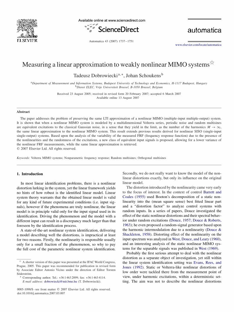
Automatica 43 (2007) 1737–1751www.elsevier.com/locate/automatica

Measuring a linear approximation to weakly nonlinear MIMO systems�

Tadeusz Dobrowieckia,∗, Johan Schoukensb

aDepartment of Measurement and Information Systems, Budapest University of Technology and Economics, H-1117 Budapest, HungarybDienst ELEC, Vrije Universiteit Brussel, B-1050 Brussel, Belgium

Received 23 August 2005; received in revised form 20 February 2007; accepted 6 March 2007Available online 13 August 2007

Abstract

The paper addresses the problem of preserving the same LTI approximation of a nonlinear MIMO (multiple-input multiple-output) system.It is shown that when a nonlinear MIMO system is modeled by a multidimensional Volterra series, periodic noise and random multisinesare equivalent excitations to the classical Gaussian noise, in a sense that they yield in the limit, as the number of the harmonics M → ∞,the same linear approximation to the nonlinear MIMO system. This result extends previous results derived for nonlinear SISO (single-inputsingle-output) systems. Based upon the analysis of the variability of the measured FRF (frequency response function) due to the presence ofthe nonlinearities and the randomness of the excitations, a new class of equivalent input signals is proposed, allowing for a lower variance ofthe nonlinear FRF measurements, while the same linear approximation is retrieved.� 2007 Elsevier Ltd. All rights reserved.

Keywords: Volterra MIMO systems; Nonparametric frequency response; Random multisines; Orthogonal multisines

1. Introduction

In most linear identification problems, there is a nonlineardistortion lurking in the system, yet the linear framework yieldsno hints of how robust is the identified linear model. Linearsystem theory warrants that the obtained linear model is validfor any kind of future experimental conditions (i.e. input sig-nals), however if the phenomena are truly nonlinear, the linearmodel is in principle valid only for the input signal used in itsidentification. Driving the phenomenon and the model with adifferent input can result in a discrepancy much larger than thatforeseen by the identification process.

A state-of-the-art nonlinear system identification, deliveringa model describing well the distortions, is impractical at leastfor two reasons. Firstly, the nonlinearity is responsible usuallyonly for a small fraction of the phenomenon, so why to paythe full cost of the parametric nonlinear system identification.

� A shorter version of this paper was presented at the IFAC World Congress,Prague, 2005. This paper was recommended for publication in revised formby Associate Editor Antonio Vicino under the direction of Editor TorstenSöderström.

∗ Corresponding author. Tel.: +36 1 463 2899; fax: +36 1 463 4114.E-mail address: [email protected] (T. Dobrowiecki).

0005-1098/$ - see front matter � 2007 Elsevier Ltd. All rights reserved.doi:10.1016/j.automatica.2007.03.007

Secondly, we do not really want to know the model of the non-linear distortions exactly, but only its influence on the originallinear model.

The distortion introduced by the nonlinearity came very earlyto the focus of interest. In the context of control Barrett andCoales (1955) used Booton’s decomposition of a static non-linearity into the (mean square sense) best fitted linear partand a “distortion factor” to analyze control systems withrandom inputs. In a series of papers, Douce investigated theeffect of the static nonlinear distortions and their spectral behav-ior under random excitations (Douce, 1957; Douce & Roberts,1963); he even proposed a random-signal generator based uponthe harmonic intermodulation due to a nonlinearity (Douce &Shackleton, 1958). Distorting effect of the nonlinearity on theinput spectrum was analyzed in West, Douce, and Leary (1960),and an interesting analysis of the static nonlinear MIMO sys-tems for the separable signals was published in West (1969).

Probably the first serious attempt to deal with the nonlineardistortion as a separate object of investigation, yet still withinthe linear system identification setting was Evans, Rees, andJones (1992). Static or Volterra-like nonlinear distortions oflow order were tackled there from the measurement point ofview, under harmonic excitations, within a deterministic set-ting. The aim was not to describe the nonlinear distortions

http://www.elsevier.com/locate/automatica

mailto:[email protected]

1738 T. Dobrowiecki, J. Schoukens / Automatica 43 (2007) 1737–1751

in general, but to get rid of them in concrete measurement situa-tions. To this purpose various harmonic signals were introduced(Evans, Rees, & Jones, 1994a, 1994b; Evans, Rees, Jones, &Hill, 1994; Evans, Rees, & Weiss, 1996), among others a spe-cial kind of multisine signals, minimizing nonlinear distortionsfor the assumed particular order of the nonlinearity (Evans,1998). Later their investigations were extended to the conceptof the best linear approximation to a Volterra system excitedby multisines with random harmonics, proposed in Schoukens,Dobrowiecki, and Pintelon (1998). Using crest-factor mini-mization introduced in Guillaume, Schoukens, Pintelon, andKollar (1991), Evans and Rees (2000a, 2000b), Solomou andRees (2003, 2004), Solomou, Rees, and Chiras (2004),and Solomou and Rees (2005) presented heuristic comparisonand analysis, indicating that the stochastic framework of therandom phase multisines is robust enough if crest-factor mini-mization is also applied. All their work was done for the SISOsystems.

Modeling nonlinear systems with their output-error lin-ear time-invariant second-order equivalents (OE-LTI-SOEs),within Gaussian and quasi-stationary framework, was intro-duced in Enqvist and Ljung (2002, 2003). The investigationfocused on the nonlinear finite impulse response (NFIR) sys-tems and a full description of stable causal OE-LTI-SOEs ofsuch systems was given by Enqvist (2005). The problem ofnonlinear distortions was addressed via the notion of slightlynonlinear system (Enqvist & Ljung, 2004). Seeking generalconditions for the SOE of an NFIR system to be also an FIRsystem, separable signals were introduced, extending the no-tion of Gaussianity (Enqvist & Ljung, 2005; Nutall, 1958).Bounds on the distance between the SOE and the linear part ofthe nonlinear system were also studied in terms of the norm.

Theoretically the most rigorous was the approach of Mäk-ilä and Partington, within the deterministic framework basedupon the Generalized Harmonic Analysis (GHA) and quasi-stationary signals, drawing upon the normed space operatortheory. In Mäkilä and Partington (2003), the Frechet deriva-tive was used to derive the best causal linear approximation ofmildly nonlinear systems (NFIR and bi-gain systems in par-ticular). Beside mean square error approximation, the absoluteerror criterion was also considered for static nonlinear systemsin Mäkilä (2003). In Mäkilä and Partington (2004) and Mäkilä(2004), the distribution theory of sequences was called in to re-fine the results obtained earlier for GHA and quasi-stationarysignals. Interesting notions of nearly linear system and its LTIcompanion were introduced in Mäkilä (2005), to investigate thecontrollability of a (NFIR) nonlinear system through the con-trol of its LTI companions. This work was extended in Mäkilä(2006a) to the linear approximations with the FIR and ARX pa-rameterization, then in Mäkilä (2006b) to the notion of a non-linear companion system, providing also state-space form forthe linear companion.

The present work is based and extends the results ofSchoukens, Dobrowiecki, and Pintelon (1995a, 1995b, 1998)and Pintelon and Schoukens (2002), where a stochastic frame-work was proposed to deal with Volterra-like nonlinear dis-tortions, randomizing the approximation errors through the

randomization of the input signals. For input signals, randomphase multisines were used. Contrary to other approaches theaim was not only to produce the “best” linear approximationto the nonlinearly distorted linear system, but to observe (andcontrol) where and how the nonlinear distortions manifestthemselves in the measured linear nonparametric frequencyresponse function (FRF); and to make a full analysis of theirstochastic behavior. The stochastic setting was essential; oth-erwise it would not be possible to qualify the error on theapproximation. The stochastic setting led to the design ofmeasurement procedures (e.g. averaging) warranting properapproximation of the theoretical limiting results (expected val-ues, infinite summations) from the finite measurement data.Such results are still due in the deterministic setting. The the-ory was developed for input signals with a finite number ofharmonics, and the asymptotic properties have been analyzedwhen the number of harmonics tends to infinity (Schoukenset al., 1998). It was also shown that asymptotically the FRFmeasured with the random multisines and periodic noise co-incide with the FRF measurements done with Gaussian noiseexcitations (Pintelon & Schoukens, 2002). All the work wasdone for the SISO systems.

Harmonic random phase signals are in the limit (in the num-ber of harmonics) normally distributed, and even separable,the measured FRF tends thus asymptotically to the FRF of theOE-LTI-SOE of a nonlinear system described by a convergentVolterra series model. However, issues like stability, causality,memory length, etc., are not considered for the nonparametricFRF. These questions are pertinent to the parametric identifi-cation, which can be made after the analysis of the measurednonparametric FRF yields hints about the frequency band, thedynamics, and the complexity of the system. It is in this suc-ceeding parametric identification step to decide whether or notthe mentioned properties should be imposed. There is also adifference between a nearly linear system (and its linear com-panion) (Mäkilä, 2005) and a weakly nonlinear Volterra se-ries. A nearly linear system, which by definition gets moreand more linear as the signal amplitude grows, does not fitwell those practical situations where the signals are bounded,but the nonlinearities (e.g. a cubic or a saturating nonlinear-ity) are not asymptotically linear. For small signals, the linearcompanion of such nonlinear system can still yield large ap-proximation errors, the best linear approximation of a weaklynonlinear Volterra series will, on the other hand, always beclosed to its linear component (Dobrowiecki & Schoukens,2002, 2004, 2006; Pintelon & Schoukens, 2001).

In the paper it is shown that the results obtained in Schoukenset al. (1998) and Pintelon and Schoukens (2002) for the SISOsystems can be extended to the MIMO systems and then newinput signals with superior properties are proposed. Section 2gives the rationale behind the choice of the system and thesignal class and reviews shortly the developed SISO theory. InSection 3 MIMO Volterra series are introduced, and in Section4 the equivalence is proven for the mentioned three classes ofsignals. In Section 6 a new class of input signals is proposed.In Section 7 some illustrative simulations and comparison ofvariances are provided with conclusions. Basic equations of

T. Dobrowiecki, J. Schoukens / Automatica 43 (2007) 1737–1751 1739

the Volterra series under harmonics excitations can be foundin Bussgang, Ehrman, and Graham (1974), Schetzen (1980),Boyd, Chua, and Desoer (1984), Billings and Tsang (1989), orLang and Billings (2000).

2. SISO theory—preliminaries

In our work convergent Volterra system series were used tomodel the problem. Their particular usefulness is dictated bya natural way, how the linear and nonlinear systems can betreated together, and the level of the nonlinearity controlled; awide class of (non-continuous) systems which can be approx-imated in the least square sense with Volterra series; a well-developed frequency-domain representation; an easy extensionof the SISO models to the MIMO models; and the possibilityto incorporate a priori physical knowledge (order, symmetry,frequency bands, etc., of the kernels).

Volterra models contain practically important nonlinearblock models, like Wiener systems, Hammerstein systems, andcascaded Wiener–Hammerstein systems. They also includeNFIR models, if we approve for the Dirac-Delta functions orKronecker-Delta symbols in the time domain kernels. As theVolterra series generalizes the Taylor expansion, their expres-siveness is limited, and there exist a number of interesting andimportant nonlinear phenomena, which cannot be modeledwell or at all with Volterra series, like bifurcations, chaos,nonlinear resonances, sub-harmonics, etc. An SISO Volterraseries in the time-domain can be described as

y(t) = V [u(t)] =∞∑

�=1

y�(t)

=∞∑

�=1

∫ ∞

−∞· · ·∫ ∞

−∞g�(�1, . . . , ��)

�∏k=1

u(t − �k) d�k ,

(1)

and in the frequency-domain for periodic inputs as

Y (l) =∞∑

�=1

Y �(l) = M−�/2∞∑

�=1

M/2∑k1,...,k�−1=−M/2

× G�(k1, k2, . . . , k�−1, k�)

�∏n=1

U(kn), (2)

where l is the discrete frequency, l = �ki , i = 1, . . . , �, y� andY � are outputs of �th order terms, g� and G� are so-called time-and frequency-domain kernels, and kernels G� are boundedby max |G�| = M� (Pintelon & Schoukens, 2002; Schoukenset al., 1998). To excite the system, periodic random signalswere adopted over non-periodic signals due to less problems inthe FRF measurements (no leakage); free hand in constructionof different signal characteristics by manipulating the spectralproperties, the frequency grid, and the phases; an easy intro-duction of the randomness (via random phases or random spec-tral amplitudes) and an easy implementation in modern signalgenerators; also the possibility to approximately model band-limited noise signals by selecting a high enough number of

harmonics in a bounded frequency band. An essential issue isthat it is easy to distinguish or to separate input signal proper-ties from the noise properties (Pintelon & Schoukens, 2001).We assume thus that the system is driven by a normalized ran-dom multisine defined as

u(t) = F−1/2∑

k=−M/2,k �=0

U (kf s/M) ej(2�kf st/M+�k)

= M−1/2M/2∑

k=−M/2,k �=0

U(k) ej2�kf st/M , (3)

U(k) = (M/F)1/2U (kf s/M) ej�k = (M/F)1/2U (k)ej�k , (4)

where the phases �k are independent identically distributed ran-dom variables uniformly distributed on [0, 2�[, with U(−k) =U(k). The function U (f ) takes nonnegative real values on(0, fmax], fmax < fS/2, and is 0 elsewhere. It is uniformlybounded, U (f )�MU < ∞, and has at most a countable num-ber of discontinuities in the band [0, fmax]. Define also U2(f )=S

UU(f ). In (3), M is an even number denoting the number of

points in the period. The frequencies fs, fmax, and the con-stant MU are independent of M. F is a natural number smallerthan M/2, but of order O(M), denoting the exact number ofnonzero harmonics in (3). Consequently, the amplitudes of thesine waves decrease as F−1/2 = O(M−1/2), and the power

1

M

M−1∑t=0

u2(tT s) =M/2∑k=1

|Uk|2 = 1

F

M/2∑k=1

U2k

is bounded by (MU)2, as there are exactly F nonzero harmonicsin (3).

For the generality of the approach no structure on the time-domain or frequency-domain kernels was imposed, besidethe boundedness of the frequency-domain kernels. The series(1)–(2) is convergent for every l, if

∑∞�=1 M�M

�U < ∞ and in

the SISO theory only systems modeled by finite Volterra series,or the limiting systems of the series (1)–(2) in the least squaresense are considered (for details see Pintelon & Schoukens,2002).

When nonlinearity is present in the system, the appearanceof its FRF changes drastically. The nonlinearity appears as asystematic “bias” and noise-like scattered “stochastic” contri-butions (see Fig. 1), which vary from one realization of the in-put to the other. If the applied input is randomized (e.g. here bythe random phases in (3)–(4)), the noise-like scatter acquiresstochastic properties and the system (1)–(2) can be modeled asa linear approximation followed by a nonlinear noise source(Schoukens et al., 1998):

Y (l) = (G0(l) + GB,M(l))U(l) + YS,M(l)

= GBLA,M(l)U(l) + YS,M(l), (5)

where GBLA,M(l) is the best linear approximation, G0(l) =G1(l) is the FRF of the true underlying linear system (if itexists), and GB,M(l) is the bias or systematic distortion term.


Fig. 1. A qualitative view of how the presence of the nonlinearity canchange the appearance of the measured FRF. To the linear system a nonlinearcomponent has been added. The FRF measured with the same input signal,in noiseless conditions, becomes noisy and shows considerable bias (right)with respect to the linear FRF (left).

The bias GB,M(l) depends only on the odd order kernels:

GB,M(l) =∞∑

�=2

G2�−1B,M (l) + O(M−1), (6)

G2�−1B,M (l)= c�

M�−1

M/2∑k1,...,k�−1=1

G�(l, k1, −k1, . . . , k�−1, −k�−1)

×�−1∏i=1

|U(ki)|2, (7)

c� = 2�−1(2� − 1)!! (8)

The nonlinear noise or stochastic distortion term YS,M(l) de-pends on all even and odd kernels, is zero mean, asymptoticallycircular complex normally distributed and mixing of arbitraryorder, and is asymptotically uncorrelated over the frequency land with input signal. The best linear approximation can bemeasured as (H1-FRF), where the expected value is taken withrespect to the random phases:

GBLA,M(l) = E{Y (l)U(l)}E{|U(l)|2} . (9)

This model has been extended to periodic noise (amplitudesU (f ) in (3) are random) and Gaussian noise excitations andtheir equivalence was shown, i.e. that the FRF and the variancevar[M−1/2YS,M(l)] of the nonlinear noise estimated with theperiodic signals tend in the mean square limit (as the numberof harmonics F →∝, or M →∝) to the same best linearapproximation of the SISO system and to the same variancevalues as measured with the Gaussian noise, provided that thesignal spectra are comparable (Pintelon & Schoukens, 2002).

From the point of view of the best linear approximation mea-surements (9), Gaussian noise in finite records introduces leak-age. The amplitude spectrum of Gaussian and periodic noisecan show dips, resulting in a high noise sensitivity of (9), andintroducing more fluctuation and even spikes into the FRF mea-surements. Comparably, the amplitude spectrum of the ran-dom multisines does not fluctuate from one realization to theother, so the denominator in (9) is constant, and the FRF esti-mate is more stable. Therefore, random multisines are proposedas signals of choice in weakly nonlinear SISO measurements(Pintelon & Schoukens, 2001). It is important to mention, thatthe approach based upon the characterization of the nonlineardistortion as a nonlinear noise source and a biased term, is validfor any convergent Volterra series.

3. MIMO Volterra systems

In this paper the SISO theory is extended to MIMO Volterrasystems without feedback, i.e. every output of the MIMO sys-tem can be described as a multiple-input single-output (MISO)system. So, without any loss of generality we can focus onMISO systems. In the time-domain, the output of the N-inputMISO system is

y(t) = V [u1(t), u2(t), . . . , uN(t)] =∞∑

�=1

y�(t)

=∞∑

�=1

∑j1j2···j�

yj1j2···j�(t). (10)

The inner sum runs over all pure and mixed �th order ker-nels, and the output of a particular �th order kernel excitedby K different input signals of indices j1, j2, . . . , j�, jk ∈{1, 2, . . . , N}, k = 1, . . . , �, not all jk necessarily different, is:

yj1j2···j�(t) =∫ ∞

−∞. . .

∫ ∞

−∞gj1j2···j�(�1, . . . , ��)

×�∏

i=1

uji(t − �i ) d�i .

In the frequency-domain, for periodic inputs the system modelis

Y (l) =∞∑

�=1

Y �(l) =∞∑

�=1

∑j1j2···j�

Y j1j2···j�(l), (11)

Y j1j2···j�(l)

= M−�/2M/2∑

k1,...,k�−1=−M/2

Gj1j2···j�(k1, k2, . . . , k�−1, k�)

×�∏

i=1

Uji(ki), (12)

where l is the discrete frequency, l =�ki , i =1, . . . , �, gj1j2···j�

and Gj1j2···j� are time and frequency kernels, respectively


(for the notation see (10)). We assume that the system inputsare driven by a normalized random multisine signal (3)–(4).

Similar to the SISO case, no special conditions are im-posed on the time-domain or the frequency-domain kernelsbesides that the frequency-domain kernels and the input sig-nals must be bounded. Kernels Gj1j2···j� are bounded by max|Gj1j2···j� |=Mj1j2···j� . The series (11) is convergent for every l,if the input signals are normalized to unit power and have uni-formly bounded spectral amplitudes |Uk|�MU,k/

√M < ∞,

and if together∑∞

�=1M�M�U < ∞ holds, where M� =

maxall � order kernels|Mj1j2···j� |, MU = maxall input signals|MU,k|.In the following only systems modeled by finite MIMO

Volterra series or systems being limits of the series (11) in theleast square sense are considered, similar to the SISO theory.In the discussion we will also assume that no other disturbingnoise sources are present on the system outputs, thus focusingthe analysis on the input signals and the nonlinear effects.

4. MIMO bias equivalent input signals

In this section we investigate how to extend the best linearapproximation model (5)–(8) to the MIMO Volterra series (11).First, the general form of the bias on the MIMO FRF is es-tablished for the random multisine excitations, and then it isshown that it is valid also for the periodic noise inputs. Takingthe limit F → ∞, it is further shown that the measurement re-sults converge to those made with Gaussian noise with a com-parable spectral behavior. By proving this equivalence we alsoshow that the output of the Volterra MIMO system (11), excitedby the periodic signals, can be written as

Y (l) =N∑

k=1

GkBLA,M(l)Uk(l) + YS,M(l), (13)

where GkBLA,M(l) = Gk(l) + Gk

B,M(l) are best linear approxi-mations (FRFs) to the nonlinear relations described by the mul-tidimensional Volterra series in the signal path Y − Uk (withexpected value taken with respect to the random phases), andGk

B,M are biases on the linear FRFs introduced by the nonlin-earity. The equivalent noise source YS,M(l), E{YS,M(l)} = 0,and E{YS,M(l)Uk(l)} = 0, for k = 1, . . . , N , captures all thenonsystematic nonlinear effects. The best linear approximationGk

BLA,M can be measured similarly to (9) as

GkBLA,M(l) = E{Y (l)Uk(l)}

E{|Uk(l)|2} . (14)

Eq. (13) yields the MIMO additive nonlinear noise sourcemodel, a straightforward extension to the SISO and two-inputtwo-output (TITO) cases (Dobrowiecki & Schoukens, 2004).The index k of the measured signal path is called in the follow-ing the “reference input index”.

In practice all the signal paths in a particular MISO systemare computed simultaneously via a set of equations. For thispurpose J independent experiments are made with independentrealizations of the input signals U(1), . . . , U(J ) (indices in theparentheses are the serial numbers of the experiments). After

the transients settle, the successive records to be processed arecut from the input and output signals. Signal amplitudes atfrequency l are then arranged into:

Y(l) = G(l)U(l) = [Y (1)(l) . . . Y (J )(l)]

= [G1(l) . . . GN(l)]

⎡⎢⎢⎣

U(1)1 (l) . . . U

(J )1 (l)

. . . U(i)j (l) . . .

U(1)N (l) . . . U

(J )N (l)

⎤⎥⎥⎦ ,

(15)

where U is so-called input matrix, a N × J matrix of complexinput amplitudes (4), G is a 1 × N matrix of the true FRFvalues for different input–output channels; Y is 1 × J matrixof the output amplitudes. We will assume also in the followingthat J = NB × N , i.e. the number of experiments is an integralnumber of N experiment blocks. We will distinguish also aspecial N × N input matrix built from J = N experiments:

UN(l) =

⎡⎢⎢⎢⎢⎣

U(1)1 (l) U

(2)1 (l) · · · U

(N)1 (l)

U(1)2 (l) U

(2)2 (l) · · · U

(N)2 (l)

· · · · · · · · · · · ·U

(1)N (l) U

(2)N (l) · · · U

(N)N (l)

⎤⎥⎥⎥⎥⎦ . (16)

The required FRF estimates Gi(l) can be computed as ((·)H isthe conjugate transpose):

G(l) = Gi(l) = Y(l)UH (l)(U(l)UH (l))−1

= SYU (l)S−1UU(l). (17)

Extending the theory from SISO to MIMO systems requiresassumptions how signals at different inputs are related to eachother. We will require that:

Assumption 1. The MIMO system can be of arbitrary but finiteinput dimension N, and an arbitrary order of the nonlinearity(assuming that the sums in (11) converge).

Assumption 2. Signals at different inputs are independent fromeach other.

Assumption 3. Signals in different experiments are indepen-dent.

We start with the general form of the bias in (13):

Theorem 1. Under Assumptions 1–3, when the system (11) ismeasured with a random multisine excitations (3), the bias termin (13) in the signal path Y − Uk is built only from those odd�th order kernels, with K different inputs, which contain thereference input k an M1 odd number of times, and any otherinput an Ml even number of times, including Ml = 0:

GkBLA,M(l) = Gk(l) +

∑� odd

∑j1j2···j�

Gj1j2···j�B (l), (18)


Gj1j2···j�B (l)= Ckernel

(F )(�−1)/2

M∑k1,...,k(�−1)/2=0

Gj1j2···j�(l, −k1, k1, . . .)

×∏n1

SUj1 Uj1

(n1)∏n2

SUj2 Uj2

(n2) · · ·

×∏nK

SUjK

UjK(nK),

(19)

Ckernel = 2(�−1)/2M1!!K∏

l=1

(Ml − 1)!!, � =K∑

k=1

Mk , (20)

where the first product is defined on (M1 − 1)/2 discrete fre-quencies from among (k1, k2, . . . , k(�−1)/2), the second prod-uct on M2/2 frequencies, etc., finally the last product on theremaining MK/2 frequencies in the summation. For the sketchof the proof see Appendix A. (Note also that the SISO case (7)(Schoukens et al., 1998) is a special case of Theorem 1 withonly the reference input, i.e. the first product present.)

To formulate the results on the equivalence of various inputsignals we need:

Assumption 4. The periodic signals Uk, k = 1, . . . , N , are de-fined on the same frequency grid, and all signals have compa-rable spectral powers in the following sense:

• for random multisines (3):

U2k (f ) = S

UU(f ); (21)

• for periodic noise: the spectral amplitudes U (f ) in (3)–(4)are random, independent over the frequencies and indepen-dent from the phases, U (f ) has uniformly bounded momentsof any order, and:

E{U2k (f )} = S

UU(f ), (22)

has a countable number of discontinuities in the frequencyband [0, fmax];

• for Gaussian noise:

SUU(f ) = SUU

(f )/fmax. (23)

Then the results on the equivalence can be collected in thefollowing theorem:

Theorem 2. Under Assumptions 1–4, with the input signalsnormalized to the same spectral behavior (21)–(23) and forthe limit M →∝, the periodic noise, and the random multi-sines yield exactly the same linear approximation to a nonlinearMIMO system described by a multidimensional Volterra series

(11), as that measured with the Gaussian noise:

GkBLA,M(l) = Gk(l) +

∑� odd

∑j1j2···j�

Gj1j2···j�B (l), (24)

Gj1j2...j�B (j�) = Ckernel

(fmax)(�−1)/2

∫ fmax

f2=0· · ·∫ fmax

f�=0

× Gj1j2···j�(f, −f2, f2, . . .)∏n1

SUj1 Uj1

(j�n1)

×∏n2

SUj2 Uj2

(j�n2) . . .∏nK

SUjK

UjK(j�nK

)

× df2 . . . df�, (25)

Ckernel = 2(�−1)/2M1!!K∏

l=1

(Ml − 1)!!,

� =K∑

k=1

Mk, � = (� + 1)

2, (26)

where the first product is defined on (M1 − 1)/2 frequenciesfrom among (f2, f3, . . . , f�), the second product on M2/2 fre-quencies, etc., finally the last product on the MK/2 frequenciesin the summation. For the sketch of the proof see Appendix B.

It remains to see that the measurement procedure (14) yieldsresults compatible with (24)–(26).

Theorem 3. Under Assumptions 1–4, the procedure (14) usedwith the periodic noise and the random multisines, yields ex-actly the same linear approximation to a nonlinear MIMO sys-tem described by a multidimensional Volterra series (11), asgiven in (24)–(26). For the sketch of the proof see Appendix C.

5. Some remarks on the variance

Even in the absence of disturbing output noise, the FRF mea-surements (14) will vary from one realization to the other fortwo reasons. One is the fluctuation of the inverse matrix in(17), due to the randomness of the excitations. Note, that thematrix (UUH )−1 fluctuates even when random multisines withconstant amplitude spectrum are used, contrary to the measure-ments on SISO systems (Pintelon & Schoukens, 2001). Othersources are zero mean stochastic contributions generated by thenonlinear noise source YS,M(l) in (13). Generally the varianceon the measured FRF is a function of the used input signalsand the particular composition of the nonlinear part of the sys-

tem. In the SISO case, SUU (l)=∑Je=1U

(e)(l)U(e)

(l) randomlyfluctuates for the noise and periodic noise excitations, but is de-terministic for the random multisine excitations. In the MIMOcase, this result would not be valid, because as mentioned ear-lier S−1

UU(l) in (17) will contain stochastic components for allthree considered input signal classes.

In the comparison of the periodic noise and the random mul-tisine, periodic noise turns out better, because its input matrixis better conditioned (see Appendix D and also Figs. 3–5, for


NB = 1). Gaussian noise, in addition, introduces leakage andyields even worse results. The aim is then to reduce further themeasurement variance by reducing the random fluctuations ofthe inverse in (17), reducing the influence of YS,M(l), whileat the same time maintaining that the bias equivalence of themeasurements with respect to all of the previous input signalsshould be kept such that GBLA in (13) is the same for allexcitations. We will attempt to solve this problem by proposinga new class of input signals.

6. Orthogonal random multisines

6.1. Introduction

In Guillaume, Pintelon, & Schoukens (1996), orthogonal in-put signals

U(l) =[

1 1

1 −1

]U(l) (27)

were introduced for linear TITO FRF measurements to atten-uate the influence of the process noise. Such a choice of exci-tation signals comes from the minimization of the uncertaintyellipsoid around the measured FRF, and is provided by the so-lution to the maximum determinant problem of Hadamard; seeBrenner & Cummings (1972).

As the SISO Volterra system, excited with random multi-sines, can be modeled as a linear approximation followed bya nonlinear output noise, and this model applies also to theMIMO systems (Section 4), orthogonal inputs (27) were ap-plied with promising results to the cubic TITO system, yield-ing much less variance in the measurements (Dobrowiecki &Schoukens, 2004). Yet direct generalization of these orthogo-nal inputs to an arbitrary MIMO system (N > 2, � > 3) doesnot work. The ideal would be an input signal matrix yieldingno fluctuation in (17) at all, defined for all values of N (inputdimension), yielding less variance but being equivalent to othernormally used input signals for any � (nonlinear order).

6.2. Definition

The N unknown FRF values at the frequency l in (15)–(17)can be computed from at least N different experiments. Let uscall it a block (of experiments) and assume that J = NB ×N experiments are made (NB is the number of blocks in theexperiments). Let us partition the N ×J input matrix U in (15)into NB blocks as: U=[UN UN . . . UN ] and Y in a similar way.Instead of

UN(l) =

⎡⎢⎢⎢⎢⎣

U(1)1 (l) U

(2)1 (l) . . . U

(N)1 (l)

U(1)2 (l) U

(2)2 (l) . . . U

(N)2 (l)

. . . . . . . . . . . .

U(1)N (l) U

(2)N (l) . . . U

(N)N (l)

⎤⎥⎥⎥⎥⎦ ,

which requires independent excitations for every input and ev-ery experiment, we propose to use

UN(l) =

⎡⎢⎢⎢⎢⎣

w11U(1)1 (l) w12U

(1)1 (l) . . . w1NU

(1)1 (l)

w21U(1)2 (l) w22U

(1)2 (l) . . . w2NU

(1)2 (l)

. . . . . . . . . . . .

wN1U(1)N (l) wN2U

(1)N (l) . . . wNNU

(1)N (l)

⎤⎥⎥⎥⎥⎦

= diag{U(1)k (l)}

⎡⎢⎣

w11 . . . w1N

. . . . . . . . .

wN1 . . . wNN

⎤⎥⎦= DU W, (28)

where wkj are entries of an arbitrary, deterministic, unitary (ororthogonal) matrix WH W=WWH =NIN , e.g. the DFT matrix,with [W]kn = e−j2�(k−1)(n−1)/N . Such signals will be referredlater on as orthogonal multisines.

The measurement procedure is thus to generate random ex-citations for the first experiment in the block of the first N ex-periments and to shift them orthogonally, accordingly to (28)for the next N − 1 experiments. If more than one block is gen-erated, each of them is initialized with another random vector[U(i)

1 U(i)2 . . . U

(i)N ]T. It is easy to see that due to the unitary

matrix W (the experiment index is omitted for clarity):

UN(l)UHN (l) =

[Uk(l)Uj (l)

N∑i=1

wikwij

]

= N [Uk(l)Uj (l)kj ] = N diag{|Uk(l)|2}, (29)

where kj is the Kronecker Delta (see also Appendix E). Fur-thermore

(UUH )−1 = (NBUN UHN )−1 (30)

and finally

G(l) = 1

NB

NB∑i=1

GN,i(l) (31)

with

GN,i(l) = YN(l)UHN (l)(UN(l)UH

N (l))−1

= 1

Ndiag{|Uk|−2}YN(l)UH

N (l) (32)

computed without taking the inverse from one block of N equa-tions.

Various unitary (orthogonal) matrices W can be proposed.For particular even N = 0 (mod 4) input dimensions Hadamardmatrices can be used, further simplifying the procedure (theycontain ±1 entries only). E.g. for the 4-dimensional systemusing matrix:

W =

⎡⎢⎢⎢⎢⎣

1 1 1 1

1 −1 1 −1

1 1 −1 −1

1 −1 −1 1

⎤⎥⎥⎥⎥⎦ ,


leads to the input matrix:

UN(l) =

⎡⎢⎢⎢⎢⎣

U1(l) U1(l) U1(l) U1(l)

U2(l) −U2(l) U2(l) −U2(l)

U3(l) U3(l) −U3(l) −U3(l)

U4(l) −U4(l) −U4(l) U4(l)

⎤⎥⎥⎥⎥⎦ .

The DFT matrix [W]kn = e−j2�(k−1)(n−1)/N is more generalin a sense that it works for an arbitrary input dimension N.Consider as an example a three-input system:

U3(l) =

⎡⎢⎢⎣

U1(l) U1(l) U1(l)

U2(l) ej 2�3 U2(l) e−j 2�

3 U2(l)

U3(l) e−j 2�3 U3(l) ej 2�

3 U3(l)

⎤⎥⎥⎦ .

As S−1UU(l) gets rid of the random fluctuations (for advantageous

condition number see Appendix E), a drop in variance should beexpected. Moreover, it turns out that the orthogonal multisineslead to exactly the same best linear approximation GBLA asmeasured with random multisines (3), consequently they areequivalent in the sense of Theorem 2 to other input signals.In addition it is also possible to reduce the variance of YS,M

by making a proper choice of wkm and by canceling somestochastic nonlinear contributions without affecting GB. Theresults can be collected in the following theorem:

6.3. Properties

Theorem 4. Under Assumptions 1–3 orthogonal random mul-tisines defined by (28) are equivalent (in the sense of Theorem 2)to the random multisines, periodic noise and Gaussian noise.When suitably normalized to the same spectral behavior (21)and in the limit M →∝, they yield exactly the same best linearapproximation GBLA. For the sketch of proof see Appendix F.

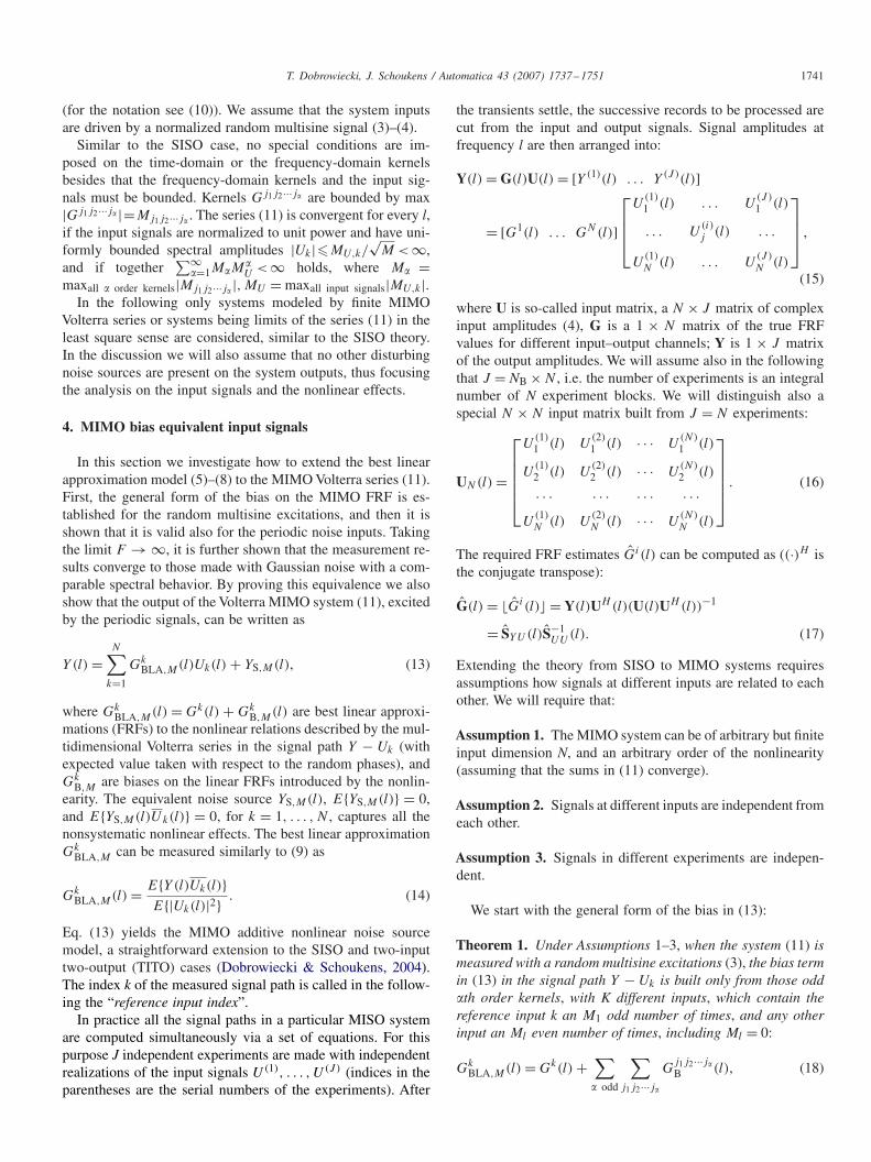
Fig. 2. The linear dynamics of the 3-dim Wiener–Hammerstein system usedin the simulations.

6.4. Discussion

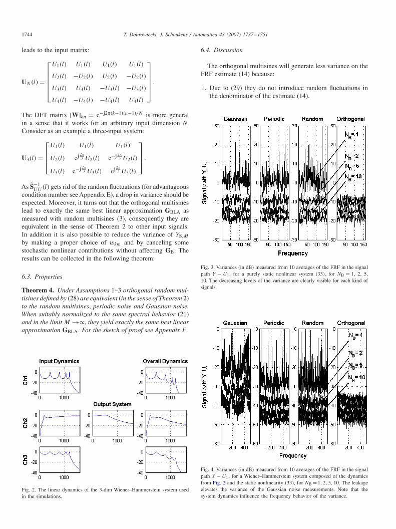
The orthogonal multisines will generate less variance on theFRF estimate (14) because:

1. Due to (29) they do not introduce random fluctuations inthe denominator of the estimate (14).

Fig. 3. Variances (in dB) measured from 10 averages of the FRF in the signalpath Y − U1, for a purely static nonlinear system (33), for NB = 1, 2, 5,10. The decreasing levels of the variance are clearly visible for each kind ofsignals.

Fig. 4. Variances (in dB) measured from 10 averages of the FRF in the signalpath Y − U1, for a Wiener–Hammerstein system composed of the dynamicsfrom Fig. 2 and the static nonlinearity (33), for NB =1, 2, 5, 10. The leakageelevates the variance of the Gaussian noise measurements. Note that thesystem dynamics influence the frequency behavior of the variance.


2. The presence of the orthogonal entries wij combined withinthe kernels leads to three possible behaviors of the zeromean (stochastic) kernel contributions, reducing further thenonlinear variance:

a. The cumulative effect of the entries wij is nonzero andfrequency-independent. Such kernels contribute to the

Fig. 5. The variance levels, averaged over the frequencies in the lower 10%of the pass-band, for the measurements on the system described in Fig. 3:Gaussian (∗) and periodic noise (O), random (X) and orthogonal multisine(�). Note the different behavior between signals randomizing the inversein (17), i.e. Gaussian noise, periodic noise and random multisines, and theorthogonal multisines, for which this matrix becomes deterministic.

Fig. 6. Variances (in dB) measured from 10 averages of the FRF for a Wiener–Hammerstein system composed of the dynamics from Fig. 2 and the staticnonlinearity (34), for NB =1, 2, 5, 10, for random and orthogonal multisines. Observe that due to the interactions between the nonlinear kernels and the unitarymatrix W, kernels which usually appear in the variance in the random multisine measurements, can drop-out in particular channels in the orthogonal multisinemeasurements (here the kernel x1 x2 does not affect the variance measured in the channel Y − U1).

nonlinear variance fully (as for random multisines, peri-odic noise and Gaussian noise).

b. The cumulative effect of the entries wij is zero andfrequency-independent. Such kernels drop out entirelyfrom the nonlinear variance.

c. The cumulative effect of the entries wij is nonzero, butfrequency-dependent. Such kernels contribute to the non-linear variance in part and is only at particular frequen-cies.

7. Simulations

For illustration a comparison is made of the nonlinear vari-ance levels measured on a 3-dim MISO system, excited withGaussian noise, periodic noise, random multisines, and orthog-onal random multisines. For the matrix W the DFT matrix waschosen. All input signals are scaled to unit power and in themeasurements NB = 1, 2, 5, 10 blocks were used (J = 3NB).The MISO system has a Wiener–Hammerstein structure withlinear input, output, and the overall dynamics shown in Fig. 2.

In the first simulation the static nonlinearity contains allmixed powers up to the fifth order:

NL = x1 + x2 + x2 + 10−2

×∑

i,j,k=0..5

xi1x

j2 xk

3 , 1 < i + j + k�5 (33)

and was designed to show the general situation with a weaklynonlinear system. As mentioned before, in the simulationsno other noise sources were considered. For the compactcomparison of the results, the actual variance measurementsand the average variance levels are presented. The variances


of the best linear approximation, measured for the nonlinear-ity (33) are shown in Figs. 3–5. Excitations that randomize theinverse in (17) show the expected rapid decrease in the vari-ance for small J. Variances measured for the orthogonal mul-tisines follow the 1/J behavior, also as expected. For a highernumber of data (blocks) all signals tend to the same limit invariance.

Variances produced with the orthogonal random multisinescan be even lower due to the drop-out effect of some kernels(see Theorem 4). This effect can be seen amplified in Fig. 6,which presents variances measured in case of:

NL = x1 + x2 + x2 + x1x2 + 10−2∑

i,j=0..5

xi1x

j2 xk

3 ,

1 < i + j + k�5. (34)

The strong nonlinear kernel x1x2 drops out entirely from theG1 measurements (Theorem 4, case a), appears fully in theG2 measurements (Theorem 4, case b), and partly in the G3

measurements (Theorem 4, case c). Please note that the drop-out effect is not influenced by the number of processed data,only by the structure of the kernels of the measured MIMOsystem.

8. Conclusions

Various practically important excitation signals yield (asthe number of harmonics increases) the same best linear ap-proximation to the Volterra SISO systems. This equivalence isextended to the nonlinear MIMO systems described by themultidimensional Volterra series. In this case, however, everykind of excitation signal will introduce random fluctuationsand an increased level of the variance on the measured FRFs.With the newly defined orthogonal multisines, the FRF mea-surements on the nonlinear MIMO Volterra systems are sig-nificantly improved in a sense that the measured MIMO FRFsG yield in the limit (as the number of harmonics in the peri-odic excitations tends to ∞) exactly the same GBLA measuredwith the traditionally used input signals, with however muchless variance 2

YrmS= E{|YS|2}. The measurement procedure is

easy; there is no need to use independent signal realizationsin every experiment, as required for the Gaussian noise, theperiodic noise and the random multisines; the procedure evendoes not require the inverting of the input matrix.

Appendix A. Proof of Theorem 1

Bias on the measured FRF is the sum of all systematic con-tributions with nonzero expected values with respect to the ran-dom inputs. As a general case we will investigate an �th orderkernel excited by K different inputs. Due to the properties ofthe random multisines:

GkBLA,M(l) = E{Y (l)Uk(l)}

E{|Uk(l)|2} = E{Y (l)Uk(l)}|Uk(l)|2 = E

{Y (l)

Uk(l)

},

i.e. it is enough to investigate the behavior of:

Gj1j2...j�B (l)

= E

{Y j1j2...j�(l)

Uk(l)

}= M−�/2

M/2∑k1,...,k�−1=−M/2

× Gj1j2...j�(k1, . . . , k�)E

{Uj1(k1) . . . Uj�(k�)

1

Uk(l)

}.

(A.1)

For the analysis the signal indices (j1, j2,…, j�) in the k ernel(12) will be grouped as:

(j1, j1, . . . , j1, j2, j2, . . . , j2, . . . , jK,jK . . . , jK, ), (A.2)

where input j1 appears in the kernel M1 times, input j2 appears

M2 times, . . . , and input jK appears MK times,∑K

l=1Ml = �,and j1 < j2 < · · · < jK . The reference input index k will beidentified usually with input index j1.

For random multisines the expectation in (A.1) applies onlyto the random phases, and due to Assumption 2, to yield nonzeroexpected value the reference input k must be present among theinputs j1, . . . , jK . Then after cancellation it must be possibleto pair the remaining inputs (phases of different inputs areindependent) to obtain terms like: U(k1)U(k2) −→

k1=−k2|U(k1)|2.

Consequently, the order M1 of the reference signal in the kernelmust be odd, and the orders Mn of other input signals even andwe have:

Gj1j2...j�B (l) = const 2(�−1)/2

(M)(�−1)/2

×M∑

k1,...,k(�−1)/2=0

Gj1j2···j�(l, −k1,k1, . . .)

×∏n1

|Uj1(n1)|2 · · ·∏nK

|UjK(nK)|2. (A.3)

The first product represent pairing of the M1 − 1 signals ofindex j1, then M2 signals of index j2, etc., finally, MK signalsof index jK . For the final form of (18)–(20) we must take intoaccount that by the symmetry of the kernels every combinationof pair-wise correlations yields the same bias. The number ofpossible combinations NR is the product of the numbers ofcombinations for input signals of the same index, i.e. NR =M1!!∏K

l=1(Ml−1)!! and we must introduce the frequency powerspectrum via (21). �

Appendix B. Proof of Theorem 2

To prove the equivalence of the input signals it is enough tocompute a single (�th order) kernel in (12), like in Theorem 1.Let us group the input signal indices as before (A.2).


B.1. Gaussian noise

The FRF measured with Gaussian noise is (H1-FRF):

GkBLA(j�k) = Gk(j�k) + Gk

B(j�k) = SYUk(j�k)

SUkUk(j�k)

.

To compute a single �th order (� = 2� − 1) contribution:

Gj1...j�B (j�k) = SYj1 ...j�Uk

(j�k)

SUkUk(j�k)

(B.1)

we need the correlation:

Ryj1 ...j�uk(�0) = E{yj1...j�(t)uk(t − �0)}

=∫ ∞

−∞. . .

∫ ∞

−∞gj1j2j ...j�(�1, . . . , ��)

× E{uk(t − �0)uj1(t − �1) . . .

× uj�(t − ��)} d�1 . . . d��.

If the reference input k is not present in j1, . . . , jK , the ex-pected value is zero, so let k = j1. Due to Assumption 2 on theindependent inputs the expected value can be written as (withsimplifying the notation of the arguments):

E{uj1uj1 . . . uj�} = E{uj1uj1 . . . uj1︸︷︷︸M1+1

}E{uj2uj2 . . . uj2︸︷︷︸M2

}

. . . E{ujKujK

. . . ujK︸︷︷︸MK

}. (B.2)

Each of the expected values in (B.2) is zero for odd numberof terms. For even number of terms they can be decom-posed into sums of combinations of pair-wise correlations��Rumum(�i−�j ), see Schetzen (1980) and Pintelon &Schoukens (2001). Consequently, the order M1 of the refer-ence signal in the kernel must be odd, and the orders Mn ofother input signals even, and let 2� − 1 = � = �i=1,...,KMi .

The �� notation means the summation over all distinct par-titions of the variables in the product into products of pair-wiseaverages. For Mk variables in the product there are (Mk − 1)!!such combinations for an even Mk . We must take now into ac-count that by the symmetry of the kernels every combinationof pair-wise correlations leads to the same bias. From (B.2) wehave:

��Ruj1uj1(�i1 − �j1) × ��Ruj2 uj2

(�i2 − �j2) × . . .

× ��RujKujK

(�iK − �jK) =

K∏l=1

��Rujlujl

(�i − �j ).

(B.3)

Eq. (B.3) can be written further as∏

inputs∑

decomp∏

Rulul(�i−

�j ) =∑NR

∏inputs

∏decompRulul

(�i − �j ). The number of pos-sible combinations NR is the product of the numbers of combi-nations at the left side of (B.3), i.e. NR = M1!!∏K

l=1(Ml − 1)!!

and we must introduce the frequency power spectra via theirFourier transforms, like in the SISO case.

We follow the philosophy of the derivation for the SISOcase (Pintelon & Schoukens, 2001), where the correlation istransformed into the bias term for a particular single partitionin (B.3) for every input signal. Other partitions yield exactlythe same bias term, due to the symmetry of the Volterra ker-nel, and the final result is thus a single computed bias termscaled up NR times. Let the particular partition be definedby (�0, �1)(�2, �3) . . . . . . ..︸︷︷︸

j1input

. . . . . . . . . . (�2�−2, �2�−1)︸︷︷︸jK input

. With this

and substituting the correlations with the Fourier transforms ofthe frequency spectra (with a simplified notation) we have:

Ryj1 ...j�uk(�0)

=∫ ∞

−∞. . .

∫ ∞

−∞gj1...jK (�1, . . . , �2�−1)e

j�1�0 e−j�1�1

× SUkUk(j�1)

�∏r=2

SUjr Ujr(j�r )e

j�r (�2r−2−�2r−1)

× d�1 . . . d�2�−1 df1 . . . df�

=∫ ∞

f1=−∞. . .

∫f�

SUkUk(j�1)e

j�1�0

�∏r=2

SUjr Ujr(j�r )

×(∫

�1

..

∫�2�−1

gj1...j�(�1, . . .)e−j�1�1

×�∏

r=2

ej�r (�2r−2−�2r−1) d�1 . . . d�2�−1

⎞⎠ df1 . . . df�.

(B.4)

Please note that a single correlation or spectrum takes placeof a product of two amplitudes in (12). Furthermore, in agreatly simplified notation the product of the spectra in (B.4)is equivalent to the product of the spectrum of the input sig-nal j1 = k on the first (M1 − 1)/2 frequencies from among(j�2, j�3, . . . , j��), multiplied by the product of the spectrumof the input signal j2 on the next M2/2 frequencies, etc., fi-nally by the product of the spectrum of the signal jK on theremaining MK/2 frequencies.

The time integral within the expression defines the multidi-mensional frequency transform of the Volterra kernel:

Gj1...jK (f, −f2,f2, . . .)

=∫�1

..

∫�2�−1

gj1j2j ...jK (�1, . . .)

× e−j�1�1

�∏r=2

ej�r (�2r−2−�2r−1) d�1 . . . d�2�−1.


With it the correlation is

Ryj1 ...j�uk(�0)

=∫ ∞

f1=−∞

(∫f2

. . .

∫f�

Gj1...jK (f, −f2,f2, . . .)

× SUkUk(j�1)

�∏r=2

SUjr Ujr(j�r ) df2 . . . df�

⎞⎠ ej�1�0 df1.

The term in the parenthesis is the required nonlinear spectralcross contribution:

SYj1 ...j�Uk(j�1)

= SUkUk(j�1)

∫f2

. . .

∫ ∞

f�=−∞Gj1...jK (f, −f2,f2, . . .)

×�∏

r=2

SUjr Ujr(j�r ) df2 . . . df�.

It remains now to scale up the cross spectrum and use (B.1) toobtain the final result (24)–(26) as

Gj1j2...j�B (j�)

= Ckernel

(fmax)(�−1)/2

∫ fmax

f2=0. . .

∫ fmax

f�=0Gj1j2...j�(f, −f2,f2, . . .)

×∏n1

SUj1 Uj1

(j�n1)∏n2

SUj2 Uj2

(j�n2) . . .

×∏nK

SUjK

UjK(j�nK

) df2 . . . df�, (B.5)

Ckernel = 2(�−1)/2M1!!K∏

l=1

(Ml − 1)!!, � =K∑

k=1

Mk

for more clarity the product of the spectra has been separatedaccording to the different input signals.

B.2. Random multisine

With the assumptions on the Volterra system and the signals,with M →∝ the sum (19) converges to the value of the integral(B.5).

B.3. Periodic noise

Consider once more (14):

GkBLA,M(l) =

EU�{Y (l)Uk(l)}

EU�{|Uk(l)|2} =

EU�{Y (l)Uk(l)}E

U{ U2

k (f )}

=E

U�{Y (l)Uk(l)}S

UU(f )

,

i.e. it is enough thus to investigate the behavior of:

Gj1j2...j�B (l) =

EU�{Y j1j2...j�(l)Uk(l)}

SUU

(f )

= S−1U U

(f )M−�/2

×M/2∑

k1,...,k�−1=−M/2

Gj1j2...j�(k1, . . . , k�)

× EU�{Uj1(k1) . . . Uj�(k�)Uk(l)}. (B.6)

For periodic noise the situation is more involved because theexpectation in (B.6) applies to both amplitudes and phases:

EU�{Uj1(k1) . . . Uj�(k�)Uk(l)}

= EU

{Uj1(k1) . . . Uj�(k�) Uk(l)}E�{ej�j1(k1) . . . e−j�k(l)}.

(B.7)

The pairing leading to the nonzero expected value is governedentirely by the pairing of the phases, so similar to the previouscase where the reference input must be present (and an oddnumber of times) in the kernel and other inputs must appear ineven numbers. In this case the phase expectation equals 1 and:

EU

{Uj1(k1) . . . Uj�(k�)} = EU

{U2j1

(k1)} . . . EU

{U2jK

(k�−1)}+ O(M−1). (B.8)

The asymptotically vanishing term contains higher even ordermoments. To create higher than second-order moments morethan 2 (4, 6, etc.) frequencies must be paired and run together.This cancels too much of degrees of freedom and together withthe normalization of the signals to the unit power yields van-ishing order of magnitude for such contributions (equivalencein the limit). Taking into account all these assumptions the biaswill again equal (A.3), and with (22) and the M →∝ will con-verge to the integral form (B.5). �

Appendix C. Proof of Theorem 3

Let Y represent for the sake of this proof the output values ofthe particular �th order kernel measured in the signal pathY–Uk ,in different experiments. When (14) is used as the measurementprocedure:

Gj1...j�B (l) = E{[Y(l)UH (l)(U(l)UH (l))−1]k}

= E

{N∑

n=1

bkn(l)

J∑i=1

Y j1...j�(i)(l)U(i)

n (l)

}

=∑

k1,...,k�−1

Gj1...j�

N∑n=1

J∑i=1

× E{U(i)j1

(k1) . . . U(i)j�

(k�)U(i)

n (l) bkn(l)}, (C.1)

where [bkn(l)] = [∑Ji=1U

(i)k (l)U

(i)

n (l)]−1.


With the phases independent over frequency and with higherthan second-order moments (pairing more than two frequenciestogether) leading to O(M−1) order contributions (see before)the internal term with expectation is

N∑n=1

J∑i=1

E{U(i)j1

(k1) . . . U(i)j�

(k�)U(i)

n (l) bkn(l)}

= |Uj1(k1)|2 . . . |Uj�−1(k�−1)|2

× E

{N∑

n=1

(J∑

i=1

U(i)k (l) U

(i)

n (l)

)bkn(l)

}. (C.2)

Please remember, that for the nonzero mean the reference in-put k must be present in the kernel an odd number of times,providing surplus amplitude after the pairing to the inner sumin (C.1). It is easy to recognize that the term in the expectationin the inner sum in (C.2) equals kn (Kronecker-Delta symbol)because it is a detailed expansion of entries of a matrix mul-tiplied by its inverse (from (17)). Substituting (C.2) into (C.1)we again obtain (A.3).

For periodic noise the expectation in (C.2) must be investi-gated according to (B.7)–(B.8), and the entries of the inversematrix pose now more problems:

N∑n=1

J∑i=1

EU,�{U(i)

j1(k1) . . . U

(i)j�

(k�)U(i)

n (l)bkn(l)}

=N∑

n=1

J∑i=1

EU

{U (i)j1

(k1) . . . U(i)j�

(k�)U(i)n (l)

× E�{ej�(i)j1

(k1) . . . e−j�(i)n (l)bkn(l)}}.

Analysis of the possible pairings which are required for thenonzero expected value leads to the interim expression of:

EU

{U2

j1(k1) . . . U2

j�−1(k�−1)

× E�

{N∑

n=1

J∑i=1

Uk(l)U(i)

n (l)bkn(l)

}},

which with the comments applying to (B.8) and (C.2) (i.e. thatthe contribution of higher order moments disappears in thelimit, that the term within expectation equals Kronecker-Deltasymbol, and with the definition of the signal spectral content(22)) yields exactly the same expression as (19). �

Appendix D. Condition number of the periodic noise andthe random multisines

Consider for illustration the case N = 2. Let

U2 =[

ej�11 ej�12

ej�21 ej�22

]and P2 =

[A11ej�11 A12ej�12

A21ej�21 A22ej�22

]

represent the input matrix (16) for the random (unit amplitude)multisines and the periodic noise, respectively, where all thephases are uniformly distributed on the unit circle and the am-plitudes Akm are exponentially distributed with unit expectedvalue. All the considered random variables are independent. Thecondition numbers become then (Golub & Van Loan, 1996):

�2(U2) = ‖U2‖2‖U−12 ‖2 = 4|ej�11ej�22 − ej�12 ej�21 |−1

= 4|ej 1 − ej 2 |−1, and (D.1)

�2(P2) = ‖P2‖2‖P−12 ‖2

=∑k,m

A2km × |B1ej 1 − B2ej 2 |−1, (D.2)

where the phases k are uniformly distributed and independent,and Bk’s are independent products of independent, exponen-tially distributed variables. Clearly for (D.2) to be singular notonly the phazors must be colineated as for (D.1), but also therandom amplitudes should match, which is an event of lowerprobability than the singularity of (D.1). Consequently, the av-erage condition number for the periodic noise will be slightlybetter.

Appendix E. Condition number of the input matrix builtfrom orthogonal random multisines

We will show that the matrix (28) has relative conditionnumber �(UN)/N = 1, for any unitary W built from the rootsof unity and for equal input spectra at different inputs. For sim-plicity we will omit the frequency and the experiment indices:

UN UHN =

⎡⎢⎢⎢⎢⎣

w11U1 w12U1 · · · w1NU1

w21U2 w22U2 . . . w2NU2

· · · · · · · · · · · ·wN1UN wN2UN . . . wNNUN

⎤⎥⎥⎥⎥⎦

×

⎡⎢⎢⎢⎢⎣

w11U1 w21U2 · · · wN1UN

w12U1 w22U2 · · · wN2UN

· · · · · · · · · · · ·w1NU1 w2NU2 · · · wNNUN

⎤⎥⎥⎥⎥⎦ .

Then from (11) [UN UHN ]kj = [UkUj

∑Ni=1wkiwji]kj =

UkUj [WWH ]kj = NkjUkUj , where kj is Kronecker-Deltasymbol. Now UN UH

N = ND, and D = diag{|Uk|2}, andUH

N = NU−1N D, and U−1

N = 1N

UHN D−1,

U−1N = 1

NUH

N × diag

{1

|Uk|2}

= 1

N

⎡⎢⎣

w11U1

|U1|2 · · · wN1UN

|UN |2· · · · · · · · ·

w1NU1

|U1|2 · · · wNNUN

|UN |2

⎤⎥⎦ . (E.1)


With the choice of the Frobenius matrix norm ‖UN‖2F =∑N

k=1∑N

j=1 |ukj |2 =∑Nk=1 |Uk|2∑N

j=1 |wkj |2 =N∑N

k=1|Uk|2.

Similarly ‖U−1N ‖2

F = · · · = 1N2

∑Nk=1|Uk|−2∑N

j=1|wkj |2 =1N

∑Nk=1|Uk|−2. The condition number becomes (Golub & Van

Loan, 1996) �(UN) = ||UN‖F‖U−1N ||F =√∑N

k=1 |Uk|2∑Nk=1 |Uk|−2. For the flat (|Uk| = const) multi-

sines � (UN) = N . The condition number becomes worse ofcourse when the input amplitude levels are not equal.

Appendix F. Proof of Theorem 4

Let Y represent for the sake of this proof the output valuesof the particular �th order kernel measured in the signal pathY–Uk , in different experiments. Due to (29)–(32) and (E.1) itis enough to show the equivalence of the FRF measured for asingle block of data (J = N). In that case

Gj1...j�B (l)

= E{[Y(l)UH (l)(U(l)UH (l))−1]k}

= E

{N∑

n=1

bkn(l)Yj1...j�(n)(l)

}

=∑

k1,...,k�−1

Gj1...j�E

{N∑

n=1

U(n)j1

(k1) . . . U(n)j�

(k�) bkn(l)

},

(F.1)

where by (28) and (E.1) U(n)j (l)=wnjUj (l), bkn(l)= wnkUk(l)

N |Uk(l)|2 ,and (F.1) can be written as

Gj1...j�B (l) = A ×

∑k1,...,k�−1

Gj1...j�(k1, . . . , k�)1

|Uk(l)|2

× E{Uj1(k1) · · · Uj�(k�)Uk(l)}. (F.2)

For the expected value to be nonzero exactly the same con-ditions on the inputs are required as before (i.e. the referenceinput present odd number of times, other inputs present evennumber of times). Coefficient A represents dependency of thebias on the choice of the particular unitary matrix W and is anessential feature of the proposed inputs:

A = 1

N

N∑n=1

�nj1�nj2 . . . �nj�vnk, �nk ={

wnk, k > 0,

wnk, k < 0.(F.3)

As the explanation please remember, that: U(n)j (−l)=U

(n)

j (l)=wnjUj (l), consequently pairing of the frequencies, which in-troduces complex conjugate to the signal amplitudes, will per-form conjugation also on entries wkn. For frequency pairingsleading to the nonzero expected value in (F.2), i.e. contributingto the bias:

A = 1

N

N∑n=1

|wnj1 |2|wnj2 |2 . . . |wnk|2 = 1

N

N∑n=1

1 = 1 (F.4)

due to |wnk|2 = 1, and the bias expression derived from (F.2)with (21) again coincides with (28).

The value of (F.3) depends naturally on the choice of theorthogonal matrix W, on the indices of the input in the kernel,on the reference signal index of the measured signal path andon the frequency pairing introducing complex conjugate forthe negative frequencies. Three cases can be distinguished ingeneral for zero expected value kernels, i.e. kernels contributingto the nonlinear variance:

a. A = 1 for all frequencies (as e.g. in (F.4)). Such kernelwill contribute fully to the nonlinear variance on the FRF.

b. A = 0 for all frequencies (if e.g. A is reduced by theproperties of W to A = 1

N

∑Nn=1 wnp for some p �= 1. Such

kernel drops out (does not contribute to) from the variance.c. A = 0 only for some frequencies (when taking complex

conjugate leads at a particular frequency to a suitable reductionin the product of the entries in (F.3)). Such kernel contributesto the variance at those frequencies only.

Please note that choosing Hadamard matrix for W excludescase c as there is no complex conjugate on the orthogonalcoefficients. �

References

Barrett, J. F., & Coales, J. F. (1955). An Introduction to the Analysis of Non-linear Control Systems with Random Inputs. The Institution of ElectricalEngineers, Monograph No. 154 M, 1955, pp. 190–199.

Billings, S. A., & Tsang, K. M. (1989). Spectral analysis for nonlinearsystems, part II: Interpretation of nonlinear frequency response function.Mechanical Systems and Signal Processing, 3(4), 341–359.

Boyd, S., Chua, L. O., & Desoer, C. A. (1984). Analytical foundations ofVolterra series. IMA Journal of Mathematical Control and Information, 1,243–282.

Brenner, J., & Cummings, L. (1972). The Hadamard maximum determinantproblem. American Mathematical Monthly, 79, 626–630.

Bussgang, J. J., Ehrman, L., & Graham, J. W. (1974). Analysis of nonlinearsystems with multiple inputs. Proceedings of the IEEE, 62, 1088–1119.

Dobrowiecki, T. P., & Schoukens, J. (2002). Cascading Wiener–Hammersteinsystems. In Proc. of the 19th IEEE instrumentation and measurementtechnology conference—IMTC’2002 (pp. 881–886), May 21-23,Anchorage, USA.

Dobrowiecki, T. P., and Schoukens, J. (2004). Linear approximation of weaklynonlinear MIMO systems. In Proc. of the 21st IEEE instrumentation andmeasurement technology conference—IMTC’2004 (pp. 1607–1612), May18–20, Como, Italy.

Dobrowiecki, T. P., & Schoukens, J. (2006). Robustness of the relatedlinear dynamic system estimates in cascaded nonlinear MIMO systems.In Proc. of the 23rd IEEE instrumentation and measurement technologyconference—IMTC’2006, April 24–27, Sorrento, Italy.

Douce, J. L. (1957). A Note on the evaluation of the response of a non-linearelement to sinusoidal and random signals. The Institution of ElectricalEngineers, Monograph No. 257 M, 1957, pp. 1–5.

Douce, J. L., & Roberts, P. D. (1963). Effect of distortion on the performanceof non-linear control systems. Proceedings of the IEE, 110(8), 1497–1502.

Douce, J. L., & Shackleton, J. M. (1958). L.F. random-signal generator.Electronic and Radio Engineer, 35(8), 295–297.

Enqvist, M. (2005). Linear models of nonlinear systems. Linköping Studiesin Science and Technology. Dissertation No. 985, Department of ElectricalEngineering, Linköping Universiteit, Linköping.

Enqvist, M., & Ljung, L. (2002). Estimating nonlinear systems ina neighborhood of LTI-approximants. Report No. LiTH-ISY-R-2459,Department of Electrical Engineering, Linköping Universiteit, Linköping.


Enqvist, M., & Ljung, L. (2003). Linear models of nonlinear FIR systemswith Gaussian inputs. In Proc. of the 13th IFAC symposium on systemidentification (pp. 1910–1915), August 2003, Rotterdam, The Netherlands.

Enqvist, M., & Ljung, L. (2004). LTI approximation of slightly nonlinearsystems: Some intriguing examples. In Proc. of NOLCOS 2004—IFACsymposium on nonlinear control systems, 2004.

Enqvist, M., & Ljung, L. (2005). Linear approximation of nonlinear FIRsystems for separable input processes. Automatica, 41(3), 459–473.

Evans, C. (1998). Identification of linear and nonlinear systems usingmultisine signals, with a gas turbine application. Ph.D. dissertation, Schoolof Electronics, University of Glamorgan, Wales, UK.

Evans, C., & Rees, D. (2000a). Nonlinear distortions and multisinesignals—part I: Measuring the best linear approximation. IEEETransactions on Instrumentation and Measurement, 49, 602–609.

Evans, C., & Rees, D. (2000b). Nonlinear distortions and multisinesignals—part II: Minimizing the distortion. IEEE Transactions onInstrumentation and Measurement, 49(3), 610–616.

Evans, C., Rees, D., & Jones, D. L. (1992). Design of test signalsfor identification of linear systems with nonlinear distortion. IEEETransactions on Instrumentation and Measurement, 41(6), 768–774.

Evans, C., Rees, D., & Jones, D. L. (1994a). Identifying linear models ofsystems suffering nonlinear distortions. In CONTROL’94, 21–24 March1994, Conference Publications No. 389, pp. 288–296.

Evans, C., Rees, D., & Jones, D. L. (1994b). Nonlinear disturbances errorsin system identification using multisine test signals. IEEE Transactions onInstrumentation and Measurement, 43(2), 238–244.

Evans, C., Rees, D., Jones, D. L., & Hill, D. (1994). Measurement andidentification of gas turbine dynamics in the presence of noise andnonlinearities. In Proc. of the IEEE instrumentation and measurementtechnology conference—IMTC’94, May 10-12, 1994, Hamamatsu, Japan.

Evans, C., Rees, D., & Weiss, M. (1996). Periodic signals for measuringnonlinear Volterra kernels. IEEE Transactions on Instrumentation andMeasurement, 45(2), 362–371.

Golub, G. H., & Van Loan, C. F. (1996). Matrix computations. (3rd ed.),Baltimore, MD: John Hopkins University Press.

Guillaume, P., Pintelon, R., & Schoukens, J. (1996). Accurate estimation ofmultivariable frequency response functions. In Proc. of the 13th IFACtriennial World conference (pp. 423–428), San Francisco, USA.

Guillaume, P., Schoukens, J., Pintelon, R., & Kollar, I. (1991). Crest factorminimization using nonlinear Chebyshev approximation method. IEEETransactions on Instrumentation and Measurement, 40(6), 982–989.

Lang Zi-Qiang, & Billings, S. A. (2000). Evaluation of output frequencyresponses of nonlinear systems under multiple inputs. IEEE Transactionson Circuits and Systems—II: Analog and Digital Signal Processing, 47(1),28–38.

Mäkilä, P. M. (2003). Squared and absolute errors in optimal approximationof nonlinear systems. Automatica, 39, 1865–1876.

Mäkilä, P. M. (2004). On optimal LTI approximation of nonlinear systems.IEEE Transactions on Automatic Control, 49(7), 1178–1182.

Mäkilä, P. M. (2005). LTI modeling of NFIR systems: Near-linearity andcontrol, LS estimation and linearization. Automatica, 41, 29–41.

Mäkilä, P. M. (2006a). On robustness in control and LTI identification: Near-linearity and non-conic uncertainty. Automatica, 42, 601–612.

Mäkilä, P. M. (2006b). LTI approximation of nonlinear systems via signaldistribution theory. Automatica, 42, 917–928.

Mäkilä, P. M., & Partington, J. R. (2003). On linear models for nonlinearsystems. Automatica, 39, 1–13.

Mäkilä, P. M., & Partington, J. R. (2004). Least-squares LTI approximationof nonlinear systems and quasistationarity analysis. Automatica, 40,1157–1169.

Nutall, A.H., (1958) Theory and Application of the Separable Class of RandomProcesses, Tech Rep 343, May 26, 1958, MIT, Research Laboratory forElectronics.

Pintelon, R., & Schoukens, J. (2001). System identification. A frequencydomain approach. Piscataway: IEEE Press.

Pintelon, R., & Schoukens, J. (2002). Measurement and modeling of linearsystems in the presence of non-linear distortions. Mechanical Systems andSignal Processing, 16(5), 785–801.

Schetzen, M. (1980). The Volterra and Wiener theories of nonlinear systems.New York: Wiley.

Schoukens J., Dobrowiecki, T.P., & Pintelon, R. (1995a). Identification oflinear systems in the presence of nonlinear distortions. A frequency domainapproach. Part I: Non-parametric identification. In Proc. of the 34th conf.on decision and control (pp. 1216–1221), December 1995, New Orleans,LA.

Schoukens J., Dobrowiecki, T.P., & Pintelon, P. (1995b). Identification oflinear systems in the presence of nonlinear distortions. A frequency domainapproach. Part II: Parametric identification. In Proc. of the 34th conf. ondecision and control (pp. 1222–1227), December 1995, New Orleans, LA.

Schoukens, J., Dobrowiecki, T. P., & Pintelon, R. (1998). Parametric andnon-parametric identification of linear systems in the presence of nonlineardistortions. A frequency domain approach. IEEE Transactions on AutomaticControl, 43(2), 176–190.

Solomou, M., & Rees, D. (2003). Measuring the best linear approximationof systems suffering nonlinear distortions: An alternative method. IEEETransactions on Instrumentation and Measurement, 52(4), 1114–1119.

Solomou, M., & Rees, D. (2004). System modeling in the presenceof nonlinear distortions. In Proc. of the IEEE instrumentation andmeasurement technology conference—IMTC 2004, 18–20 May 2004 (pp.1601–1606), Lake Como, Italy.

Solomou, M., & Rees, D. (2005). Frequency domain analysis of nonlineardistortions on linear frequency response function measurements. IEEETransactions on Instrumentation and Measurement, 54(3), 1313–1320.

Solomou, M., Rees, D., & Chiras, N. (2004). Frequency domain analysis ofnonlinear systems driven by multiharmonic signals. IEEE Transactions onInstrumentation and Measurement, 53(2), 243–250.

West, J. C. (1969). The equivalent gain matrix of a multivariable non-linearity.Measurement and Control, 2, T1–T5.

West, J. C., Douce, J. L., & Leary, B. G. (1960). Frequency spectrumdistortion of random signals in non-linear feedback systems. The Institutionof Electrical Engineers, Monograph No. 419 M, 1960, pp. 259–264.

Tadeusz Dobrowiecki was born in Warsaw,Poland, on January 25, 1952. He received hisM.Sc. degree in electrical engineering in 1975from the Technical University of Budapest,and Ph.D. (candidate of sciences) degree fromthe Hungarian Academy of Sciences, in 1981.After spending 1 year as a professional systemengineer, he joined the staff of the Depart-ment of Measurement and Information Sys-tems, Budapest University of Technology andEconomics, where he is working ever since,

currently as an Associate Professor. His research interests concern advancedsignal processing algorithms and knowledge intensive problems in measure-ment and system identification.

Johan Schoukens received the Engineering de-gree and the degree of doctor in Applied Sci-ences both from the Vrije Universiteit Brussel(VUB), Brussle, Belgium, in 1980 and 1985,respectively. He is currently a Professor at theVUB. The prime factors of his research are inthe field of system identification for linear andnonlinear systems. Dr. Shoukens received fromthe IEEE Instrumentation and Measurement So-ciety the Best Paper Award in 2002 and theSociety Distinguished Service Award in 2003.

Measuring a linear approximation to weakly nonlinear MIMO systems

Documents

Transcript of Measuring a linear approximation to weakly nonlinear MIMO systems