Mathematical Modelsof

Wound Healing

Jonathan Adam Sherratt

Lincoln College

Oxford

A thesis submitted in partial fulfilment of the requirements

for the degree of Doctor of Philosophy at the University of Oxford

Trinity Term 1991

Abstract

Jonathan Adam Sherratt Thesis submitted forthe degree of D.Phil.

Lincoln College, Oxford Trinity term 1991

Mathematical Models of Wound Healing

The complex mechanisms responsible for mammalian wound healing raise many bio­ logical questions that are amenable to theoretical investigation. In the first part of this thesis, we consider the role of mitotic auto-regulation in adult epidermal wound heal­ ing. We develop a reaction-diifusion model for the healing process, with parameter values based on biological data. The model solutions compare well with experimental results on the normal healing of circular wounds, and we analyse the solutions in one spatial dimension as travelling waves. We then use the model to perform 'mathemat­ ical experiments' on the effects of adding mitosis-regulating chemicals and of varying the initial wound shape.

Recent experiments suggest that in embryos, epidermal wound healing occurs not by lamellipodial crawling as in adults, but rather by contraction of a cable of filamentous actin at the wound edge. We focus on the formation of this cable as a response to wounding, and develop and analyse a mechanical model for the post- wounding equilibrium in the microfilament network. Our model reflects the well- documented phenomenon of stress-induced alignment of actin filaments, which has been neglected in previous mechanochemical models of tissue deformation. The model solutions reflect the key aspects of the experimentally observed response to wounding.

In the final part of the thesis, we consider chemokinetic and chemotactic control of cell movement, which play an important role in many aspects of wound healing. We propose a new model which reflects the underlying receptor-based mechanisms, and apply it to endothelial cell movement in the Boyden chamber assay. We compare our model with a simpler scheme in which cells respond directly to gradients in extracellular chemical concentration, and for both models we use experimental data to make quantitative predictions on the values of the transport coefficients.

Acknowledgements

I would like to express my deep gratitude to Prof. J. D. Murray, who supervised

the first part of my doctoral research, and without whose guidance and inspiration

this thesis would not have been possible, and to Dr. P. K. Maini, whose help and

support during his supervision of the last part of the work has been invaluable. I have

been very fortunate to have the opportunity of working directly with experimental

biologists in the course of my research, and I am very grateful to Dr. Julian Lewis

(ICRF, Oxford), Dr. Paul Martin (Dept. of Human Anatomy, University of Oxford)

and Dr. Helene Sage (Dept. of Biological Structure, University of Washington) for

our numerous discussions. I am also grateful to my fellow graduate students, who

have made the Centre for Mathematical Biology such an enjoyable and productive

place to work: Debbie Benson, Daniel Bentil, Meghan Burke, David Crawford, Ger-

hard Cruywagen, Mick Jenkins, Mark Lewis, Gideon Ngwa, Robert Payne, Faustino

Sanchez-Garduno and Louisa Shaw. I have learned a great deal from talking to our

many visitors, and I would particularly like to thank Dr. Wendy Brandts (Dept. of

Physics, University of Toronto), Dr. Peter Monk (Dept. of Mathematical Sciences,

University of Delaware) and Dr. James Sneyd (Dept. of Biomathematics, UCLA).

At a more specific level, I am indebted to Jeremy Martin (Oucs) for help with

the Simpleplot package, Malcolm Austin (Oucs) for help with Figure 4.14, Tom Mi-

lac (Dept. of Applied Mathematics, University of Washington) for initial help with

computing, Dr. Katherine Sprugel (Zymogenetics, Seattle) for introducing me to the

Boy den Chamber assay, Dr. Paul Martin for providing the photographs in Figures 3.1

and 3.2, and Prof. J. Kevorkian (Dept. of Applied Mathematics, University of Wash­

ington) for excellent instruction in singular perturbation theory. My doctoral research

was funded by a graduate studentship from the Science and Engineering Research

Council of Great Britain. Finally, sincere thanks to my family and Seana for all their

support and encouragement, which has at times made all the difference.

Contents

Introduction 1

1 Models of Adult Epidermal Wound Healing 7

1.1 Biological Background .......................... 7

1.2 A Basic Model .............................. 8

1.2.1 Nonlinear cellular diffusion .................... 11

1.3 Biochemical Regulation of Mitosis: an Improved Model ........ 13

1.4 Linear Analysis and Parameter Values ................. 20

1.5 Numerical Solution of the Improved Model ............... 22

1.6 Travelling Wave Solutions ........................ 27

1.6.1 Solutions with A = oo ...................... 29

1.6.2 Solutions with D = 0 ....................... 35

2 Mathematical Experiments and Implications for Wound Geometry 45

2.1 Addition of Chemicals .......................... 45

2.2 Model Solutions for General Wound Geometries ............ 49

2.3 Quantifying Wound Shape ........................ 54

2.4 Conclusions ................................ 70

3 The Response of Embryonic Epidermis to Wounding: a Basic Model 71

3.1 Biological Background .......................... 71

3.2 The Mechanical Approach to Modelling ................. 74

3.3 One-Dimensional Solutions ........................ 80

3.3.1 Existence and uniqueness of solutions .............. 81

3.3.2 Numerical solutions ........................ 88

3.4 Two-Dimensional Radially Symmetric Solutions ............ 91

3.4.1 Solutions with constant traction ................. 93

3.4.2 Solutions with variable traction ................. 99

3.5 Singular Perturbation Analysis of the Case of Constant Traction . . . 101

3.5.1 Possible rescalings ........................ 102

3.5.2 Matching to leading order .................... 105

3.5.3 Higher order corrections ..................... 108

3.5.4 Intermediate terms and conclusions ............... 112

4 Extending the Model: the Formation of the Actin Cable 117

4.1 The Need for an Improved Model .................... 117

4.2 Stress Alignment of Actin Filaments .................. 119

4.2.1 A detailed model of filament alignment ............. 124

4.2.2 The value of k ........................... 127

4.3 Solutions of the Improved Model .................... 131

4.3.1 One-dimensional solutions .................... 131

4.3.2 Two-dimensional radially symmetric solutions ......... 132

4.4 The Critical Upper Limit on /3 ...................... 135

4.5 Appropriate Parameter Values ...................... 140

4.6 Conclusions ................................ 144

5 Chemical Control of Cell Movement and the Boyden Chamber As­

say 150

5.1 Biological Background and Previous Models .............. 150

5.2 Shortcomings of the Keller-Segel Approach, Highlighted by the Boyden

Chamber Assay .............................. 152

5.3 An Improved Model ............................ 162

5.3.1 Application to the Boyden chamber assay ........... 165

5.3.2 Parameter values ......................... 167

5.3.3 Nondimensionalization ...................... 168

5.4 Numerical Methods of Solution ..................... 172

5.5 Application of the Improved Model to the Boyden Chamber Assay . . 178

5.6 Conclusions ................................ 186

References 187

Introduction: the Biology of Wound Healing

Adult mammalian skin is composed of two parts, as illustrated in Figure 0.1.

The outer part is called the epidermis, and consists of several layers of cells. The

columnar basal cells undergo frequent mitosis to renew the layers above, and as layers

are displaced upwards by these new generations of cells, the tough, fibrous protein

keratin accumulates in their interior. The keratin gradually replaces cytoplasm until

the cells die, when they are said to be 'keratinized' or 'cornified'. Such cells constitute

the external layer of the epidermis, and are gradually sloughed.

Beneath the epidermis is the dermis. They are separated by a basal lamina, and

the junction is not flat, but rather has projections of epidermis down into the dermis,

known as 'rete ridges', which help to anchor the epidermis (Peacock, 1984). The

dermis contains blood vessels, which are not present in the epidermis, nerves, collagen

fibres, elastin fibres, pigment cells, fat cells, and fibroblasts. These are embedded in

'ground substance', an amorphous mixture of water, electrolytes, glycoproteins and

proteoglycans (Irvin, 1984). In humans, the thickness of the dermis varies from

about 1mm on the scalp to about 4mm on the back; the epidermis is about O.lmm

thick (Odland, 1983). Beneath the dermis, but not sharply delimited from it, is a

'subcutaneous layer'. This consists predominantly of fat cells, with blood vessels and

nerves also present. It is not considered to be part of the skin.

Mammalian skin contains many hairs. These grow by rapid proliferation of cells

in the hair follicle, which, although an epidermal structure, is sunk into the dermis

(Figure 0.1); the hair shaft consists of keratinized cells. There are also a wide variety

of glands in mammalian skin. In particular, sweat and sebaceous glands can act as

sources of epidermal cells after wounding (see page 7).

The overall features of the healing of a full depth wound in mammalian skin are

represented in Figure 0.2. The immediate response to injury is vascular. Blood ves-

fU*

Figure 0.1: A diagrammatic representation of a section through adult mammalian skin.

sel disruption leads to extravasation of blood and blood coagulation, as reviewed by

Dvorak et a/. (1988) and Furie and Furie (1988). This results in the formation of

a blood clot (Figure 0.2b) composed of cross-linked fibrin, fibronectin and platelets,

that together entrap plasma water, plasma proteins and blood cells, principally ery-

throcytes. Thus the blood clot is an insoluble water-binding gel (Dvorak et a/., 1988).

As the blood clot forms, several types of leukocytes (white blood cells) migrate into

the wound, in response to a variety of chemotactic factors (Leibovich and Wiseman,

1988). Neutrophils arrive first, and their primary function is the removal of con­

taminating bacteria, by phagocytosis and intracellular killing (Clark, 1989). Shortly

afterwards, monocytes appear. Upon leaving the blood and entering tissue, these cells

differentiate into active phagocytes called macrophages (Gordon, 1986). Macrophages

play a much more important role in wound healing than neutrophils: in addition to

phagocytosis, they are an important source of regulatory biochemicals (Grotendorst

£ttfc£*/*f/S

£>£*Af/s

Figure 0.2: A diagrammatic representation of the healing of mammalian skin wounds, (a) Immediately after injury, (b) The blood clot has formed, (c) The upper portion of the blood clot has dessicated, giving a scab; neovasculature has formed by angio- genesis, and fibroblasts have invaded the lower portion, forming granulation tissue. (Continued overleaf).

Figure 0.2: A diagrammatic representation of the healing of mammalian skin wounds (continued), (d) Epidermal migration and wound contraction in progress, (e) Epi­ dermal migration and wound contraction complete, (f) Scar tissue has formed and most of the scab has been sloughed.

et a/., 1988; Sprugel et a/., 1987).

With time, the upper portion of the blood clot dessicates to form the scab, which

gradually sloughs during the remainder of the healing process (Dvorak et a/., 1988).

The lower portion of the clot becomes 'granulation tissue' (Figure 0.2c). This is the

fundamental constituent of the healing wound, and consists of a dense population

of macrophages, fibroblasts and neovasculature embedded in a loose matrix of col­

lagen, fibronectin and hyaluronic acid (McDonald, 1988). Fibroblasts migrate into

the wound space in response to a number of growth and chemotactic factors released

by the platelets and macrophages present in the blood clot (Barnes, 1988; Wahl and

Alien, 1988). Much of the extracellular matrix of granulation tissue is secreted by

fibroblasts (Nusgens et a/., 1984), and they also play a major role in matrix orga­

nization, via traction morphogenesis (Harris et a/., 1981). Simultaneously to this

fibroblast influx, neovasculature forms by angiogenesis, that is, capillary buds sprout

from blood vessels adjacent to the wound. This process depends on phenotype alter­

ation, migration and proliferation of endothelial cells, and results in a rich vascular

supply in granulation tissue (Madri and Pratt, 1988).

As granulation tissue forms, the two processes of wound closure begin (Fig­

ure 0.2d). These are epidermal migration, in which epidermal cells spread across

the wound between the scab and the granulation tissue, and wound contraction, in

which the granulation tissue contracts, causing the wound edges to move inwards.

Their relative contributions to closure depend on a variety of factors, such as species,

size and site of wound (Peacock, 1984; Snowden et a/., 1984). Wound contraction is

caused by fibroblasts, which undergo a phenotype change as they migrate into the

wound space, forming contractile 'myofibroblasts'. The synchronized contraction of

these myofibroblasts, which resemble smooth muscle cells, causes the granulation tis­

sue to contract (Bereiter-Hahn, 1986; Skalli and Gabbianni, 1988). Once the wound

has closed, granulation tissue becomes known as scar tissue (Figure 0.2f). From

the time of deposition, the extracellular matrix of granulation tissue changes con­

tinuously, and this process continues in scar tissue for many months (Clark, 1988;

Compton et a/., 1989; Forrest, 1983).

In Chapters 1 and 2 of this thesis, we develop a reaction-diffusion model for the

healing of epidermal wounds in adult mammalian skin, which has direct application

to the process of epidermal migration. Recent experiments in Oxford (Martin and

Lewis, 1991a,b) suggest that in embryonic epidermal wounds, the healing mechanism

is quite different from that in adults. In Chapters 3 and 4 we use a mechanical

model to investigate one aspect of the 'purse string' mechanism proposed by Martin

and Lewis (1991a,b). Finally, in Chapter 5 we propose a new model for chemically

modulated cell movement. The processes of chemotaxis and chemokinesis are cru­

cial to many aspects of wound healing, in particular the influx of neutrophils and

monocytes during the initial 'inflammation' phase of healing, and the movement of

fibroblasts and endothelial cells into the wound space during granulation tissue for­

mation. In Chapter 5 we focus on endothelial cells, but a detailed model of chemically

controlled cell movement is an important first step in a theoretical understanding of

many aspects of the wound healing process.

Chapter 1

Models of Adult Epidermal Wound Healing

1.1 Biological BackgroundWe have described in the Introduction the role of epidermal migration in the healing

of full depth wounds in adult mammalian skin. When only the epidermis is injured,

epidermal cells again spread across the wound, but without the much more compli­

cated processes of dermal wound healing. Thus epidermal wounds provide a relatively

simple context in which to study epidermal migration, a process that is only partially

understood. Normal epidermal cells are non-motile, but in the neighbourhood of the

wound they undergo marked phenotype alteration ('mobilization') that gives them

the ability to move via lamellipodia (Clark, 1989). The main factor controlling cell

movement seems to be contact inhibition (Irvin, 1984; Bereiter-Hahn, 1986), although

chemotaxis and contact guidance may also be involved (Clark, 1988). Remnants of

glands and hair follicles can act as sources of migrating cells, in addition to the wound

edges (Winter, 1972; Rudolph, 1980).

Two mechanisms have been proposed for the movement of the cell sheet. In the

'rolling mechanism', the leading cells are successively implanted as new basal cells,

and other cells roll over these (Krawczyk, 1971; Winstanley, 1975; Ortonne et a/.,

1981). In the 'sliding mechanism', on the other hand, the cells in the interior of

the sheet respond passively to the pull of the marginal cells, although all of the

migrating cells do have the potential to be motile, since if a gap opens up in the

migrating sheet, cells at the boundary of the gap develop lamellipodia and move

inwards to close it (Trinkaus, 1984). Though the morphological data of mammalian

epidermal wound healing are convincingly explained by the rolling mechanism (Stenn

and DePalma, 1988), unequivocal evidence is lacking, whereas the sliding mechanism

is well documented in simpler systems such as amphibian epidermal wound closure

(Radice, 1980).

Soon after the onset of epidermal migration, mitotic activity increases in a band of

epidermis near the wound edge, about 1mm wide, providing an additional population

of cells (Bereiter-Hahn, 1986; Jensen and Bolund, 1988; el-Ghorab et a/., 1988). The

greatest mitotic activity is actually at the wound edge, where it can be as much as

15 times the rate in normal epidermis (Winter, 1972; Danjo et a/., 1987); activity

decreases rapidly across the band, going away from the wound. The stimulus for this

increase in mitotic activity is uncertain. Two factors that are certainly involved are

the absence of contact inhibition, which applies to mitosis as well as to cell motion

(Clark, 1988), and change in cell shape: as the cells spread out they become flatter,

which tends to increase their rate of division (Folkman, 1978; Watt, 1988). There is

experimental evidence for the production by epidermal cells of chemicals that regulate

mitosis, but we postpone discussion of this to Section 1.3.

1.2 A Basic ModelAs a first step in the modelling process, we develop in this section a model for epider­

mal wound healing under the assumption that all biochemical effects are constant.

The governing equation we use is therefore a single conservation equation for cell

density n(r, t) at position r and time i, with the general form

Rate of increase = Cell -|- Mitotic of cell density migration generation.

Following previous deterministic models of epithelial morphogenesis, which are re­

viewed in detail by Murray (1989), we represent cell migration as a linear diffusive

flux, and we take cell proliferation to be reasonably described by a logistic form,

vn(\ — n/no), where v is the linear growth rate and HQ is the unwounded cell density.

This is a commonly used metaphor for simple growth in population biology models.

Thus our model isdn __, / n \ = £>V2 n + vn (l - , Ot \ no/

8

where D is the cellular diffusion coefficient, which we assume to be a (positive)

constant. The appropriate initial condition is n — 0 inside the wound, with boundary

condition n = HQ for all t on the wound boundary. We treat the epidermis as two-

dimensional since its thickness is about 10~2 cm (Odland, 1983), while the wounds we

consider have linear dimensions of about 1cm.

To clarify the roles of the parameters, we nondimensionalize the model using

a time scale l/i/, which is of the order of magnitude of the cell cycle time, and

a length scale L, a characteristic linear dimension of the wound. For the circular

wounds considered below, we take L to be the wound radius. We define the following

dimensionless quantities, denoted by *:

n* = n/n0 r* = r/L t* = vt D* = D/(vL2 ) .

With these definitions, the dimensionless equation is, dropping the asterisks for no-

tational simplicity,flTt^ = £>V2 n + n(l-n) (1.1)

with initial condition n — 0 inside the wound and boundary condition n — 1 for all t

on the wound boundary. For circular wounds, the wound boundary is simply |r| = 1.

Equation (1.1) is the Fisher equation. We expect the solution to have the form

of a wave of cells moving across, and eventually closing, the wound. Travelling

wave solutions of the Fisher equation in an infinite one-dimensional spatial domain

have been studied extensively, and this work is summarized by Murray (1989). In

particular, when dn(x, 0)/dx = 0 except on a finite region, the dimensionless wave

speed is 2vD (Kolmogoroff et a/., 1937) and the wave form is stable to small finite

domain perturbations (Canosa, 1973).

We solved equation (1.1) numerically in a radially symmetric cylindrical geometry

for a range of values of D, using the method of lines on a uniform space mesh, and

solving the resulting system of ordinary differential equations using Gear's method,

which is a numerical scheme based on the Adams-Bashforth-Moulton method (Lam­

bert, 1973). A typical solution is illustrated in Figure 1.1. As expected intuitively,

the solution has the form of a wave of cells moving across the wound. As suggested

n(r,t) at equally-spaced times Wound Radius (-) Compared to Data (1,2)Wound Radius

«d

CM0

0.0 0.2 0.4 . 0.6 0.8 80 100Time / %

Figure 1.1: Numerical solution of equation (1.1) with D — 10~3 , which is a biologically reasonable dimensionless value (see Section 1.5). We also plot the corresponding decrease in wound radius with time, expressed as a percentage of total healing time, and compare this to data from Van den Brenk (1956). The agreement between the model solutions and experimental data is poor.

by the analysis of one-dimensional travelling wave solutions of the Fisher equation

discussed above, the dimensionless wave speed of about 0.056 in the middle part of

healing is of the same order of magnitude as 1^/D w 0.063.

Experimental studies of the healing of circular epidermal wounds, which are dis­

cussed more fully in Section 1.5, reveal that the process is biphasic. There is an initial

"lag phase', after which the wound radius decreases linearly with time. To capture

the concept of 'wound radius' from our model, we take the wound as 'healed' when

the cell density reaches 80% of its unwounded level, that is, when n = 0.8 for the

dimensionless equations. The model prediction of the decrease in wound radius with

time is illustrated in Figure 1.1, and is compared to the experimental data of Van

den Brenk (1956), one of the more careful quantitative studies of epidermal wounds.

The agreement between the model solutions and this data is poor; in particular, the

model fails to capture the biphasic nature of the healing process.

10

1.2.1 Nonlinear cellular diffusion

Given the poor comparison between the numerical solutions of (1.1) and experimen­

tal data, we now consider representing cell migration as a nonlinear diffusive process.

Biologically, the main factor controlling cell migration seems to be contact inhibition

(Irvin, 1984; Bereiter-Hahn, 1986), which could give rise to nonlinearities. Specifi­

cally, we take the diffusion coefficient as proportional to (n/no)p with p > 0, which is

a form often used in models of insect dispersal (Okubo, 1980; Murray, 1989). Using

the nondimensionalization discussed above, the dimensionless model is thus

~ = D V [n'Vn] + n(l - n) . (1.2)C/6

The initial and boundary conditions remain n = 0 inside the wound at t = 0, and

n — 1 on the wound boundary for all t.

We solved this new equation numerically in radially symmetric plane polar co­

ordinates, again using the method of lines and Gear's method. For a wide range of

values of p and Z), the form of the solution was of a front of cells moving into the

wound (Figure 1.2). Again we compared the model solutions to data from Van den

Brenk (1956). The fit with the data improved somewhat as p increased; however,

as in the case of linear cell diffusion, the solutions lack the characteristic 'lag phase

followed by linear phase' behaviour.

A phenomenon characteristic of nonlinear diffusion is the existence of waiting time

fronts, that is, solutions in which a front that is present in the initial condition moves

only after a finite waiting time (Lacey et a/., 1982; Kath, 1984). Since our numerical

solutions have the form of moving fronts, we consider the relevance of waiting time

behaviour to the solutions of (1.2).

Extending the work of Knerr (1977), Aronson et al. (1983) showed that when the

equation

dtis subject to an initial condition of the form

11

n(r,t) at equally-spaced times Wound Radius (-) Compared to Data (1,2)Wound Radius

80 100Time / %

Figure 1.2: Numerical solution of equation (1.2) with p = 4 and D = 10~3 , which is a biologically reasonable dimensionless value (see Section 1.5). We also plot the corresponding decrease in wound radius with time, expressed as a percentage of total healing time, and compare this to data from Van den Brenk (1956). The agree­ ment between the model solutions and experimental data remains poor, despite the introduction of nonlinear diffusion.

for some x0 , the solution has a non-zero finite waiting time if u, ~ (x — Xo) 2/p as

x —> x£. If U{ ~ (x - XO ) Q with a < 2/p, there is no waiting time, while if a > 2/p

there is a long waiting time, although in their investigation of a family of similarity

solutions, Lacey et al. (1982) found that in this last case all solutions appeared to

blow up with time.

Returning to the reaction-diffusion equation (1.2), the initial condition is of the

form (1.4). Further, near the edge of the front, n is small while its derivatives are

large. Thus we expect intuitively that the waiting time properties of the solution

will be approximately the same as for equation (1.3). Of course, (1.2) is in a ra­

dially symmetric cylindrical geometry while (1.3) is in a one-dimensional geometry;

the numerical simulations below suggest that this does not affect the waiting time

behaviour, as expected from simple geometrical considerations.

Now in the numerical simulations we treat n(r, 0) as composed of line segments.

Thus in the notation of Aronson et al. (1983) described above, a = 1, so that the

12

case in which we expect a waiting time is p > 2. This is confirmed by numerical

solutions, obtained as above except that we took n(r, 0) as increasing linearly from 0

to 1 on 0.95 < r < 1.0, rather than between the penultimate mesh point and r = 1.

Figure 1.3 shows the details of the initial movement of the front when p = 1, 2, 3 with

D = 10~3 in each case. There is a waiting time for p = 2, 3 but not for p = 1.

We also investigated the effect that varying the form of the initial conditions has

on the waiting time behaviour. Specifically, we used

° 0<r< 0.95( m -' ~ [(r - 0.95)/0.05] a , 0.95 < r < 1 .

In this notation, the previous simulations have a = 1. Figure 1.4 shows the numerical

solutions with p = 2 and a = 0.5, 1,2. As expected from the results of Aronson et al

(1983), there is a waiting time only for a = 1,2.

The dependence of the movement of the front on the exact form of the initial

condition, which is not dictated biologically, is a further shortcoming of the model.

1.3 Biochemical Regulation of Mitosis: an Im­ proved Model

The models presented in the previous section are inadequate for describing epidermal

wound healing. The model solutions lack the characteristic 'lag phase followed by

linear phase' form, and in the case of nonlinear diffusion, the waiting time behaviour

depends on the precise form of the initial conditions. Biologically, this suggests that

biochemical mediators are fundamental to the process of epidermal wound healing.

In the remainder of this chapter and Chapter 2, we focus on the role of chemical

auto-regulation of mitosis in the healing process. There is experimental evidence,

which we now briefly review, for the production by epidermal cells of both chemicals

that inhibit mitosis and chemicals that stimulate it.

The former are 'chalones', a generic term for inhibitors of cell proliferation that are

produced by the cell types on which they act. Although the term itself is somewhat

out of vogue (Iversen, 1985), the evidence for such inhibitory growth regulators is

13

n(r,t) for p=1 n(r,t) for p=2

CJd

o d

m 6

p o

0.90 0.92 0.94 0.96 0.98 1.00 0.90 0.92

n(r,t) for p=3

0.94 0.96 0.98 1.00

c\i d

o d

0.90 0.92 0.94 0.96 0.98 1.00

Figure 1.3: Numerical simulations of the initial movement of the wave front for equation (1.2). We plot cell density n against radius r at equally spaced times for p = 1,2,3, with D - 10~3 in each case. There is a waiting time for p = 2,3 but not for p = 1.

14

n(r,t) for alpha=0.5 n(r,t) for alpha=1

m d

CsJc>

o d

eg o

od

0.90 0.92 0.94 0.96 0.98 1.00

i

0.90

I

0.92 0.94 0.96 0.98 1.00

n(r,t) for alpha=2

m d

OJd

o d

0.90 0.92 0.94 0.96 0.98 1.00

Figure 1.4: Numerical simulations of the initial movement of the wave front for equation (1.2). We plot cell density n against radius r at equally spaced times for a - 0.5,1,2, with D = 10~3 in each case. There is a waiting time for a = 1,2 but not for a = 0.5.

15

now considerable in a wide range of cell types (Iversen, 1981, 1985). In particular,

epidermal chalones are well documented in a number of mammalian species (Marks,

1973; Fremuth, 1984; Elgjo et a/., 1986a,b; Richter et a/., 1990). There are few direct

experimental studies on the role of chalones in wound healing, although Yamaguchi

et al. (1974) used epidermal wounds to investigate chalone inhibition of mitosis in

mice.

Evidence for auto-activation of epidermal mitosis comes from two types of ex­

periment. Firstly, epidermal cell extracts and exudates have been found to increase

proliferation and healing rates in epidermal wounds, without identification of a par­

ticular active ingredient (Eisinger et a/., 1988a,b; Madden et a/., 1989). Also, specific

reagents which are known to be produced by epidermal cells have been found to in­

crease the mitotic rate of these cells, including type alpha transforming growth factor

(Coffey et al., 1987) and fibroblast growth factor (O'Keefe et a/., 1988; Halaban et

ai, 1988).

Given the considerable biological evidence for biochemical auto-regulation of epi­

dermal mitosis, we develop a model in which a single chemical, produced by epider­

mal cells, regulates the proliferation of these cells. The general form of the governing

equations we use is

Rate of increase = Cell + Mitotic . Natural of cell density migration generation loss

Rate of increase of = Diffusion + Production Decay of chemical concentration by cells active chemical.

As in the previous section, we treat the epidermis as two-dimensional. We con­

sider two cases, one in which the chemical activates mitosis, and the other in which

it inhibits it. We use linear Fickian diffusion to represent both cell migration and

chemical diffusion; the good agreement with experimental data, described in Sec­

tion 1.5, suggests that any nonlinearities in the diffusive spread of epidermal cells are

not fundamental to the healing process. For the four reaction terms, we consider the

mathematical representation of each term separately.

16

Activator Inhibitor

f(n)

lambda .cO

lambda .cO

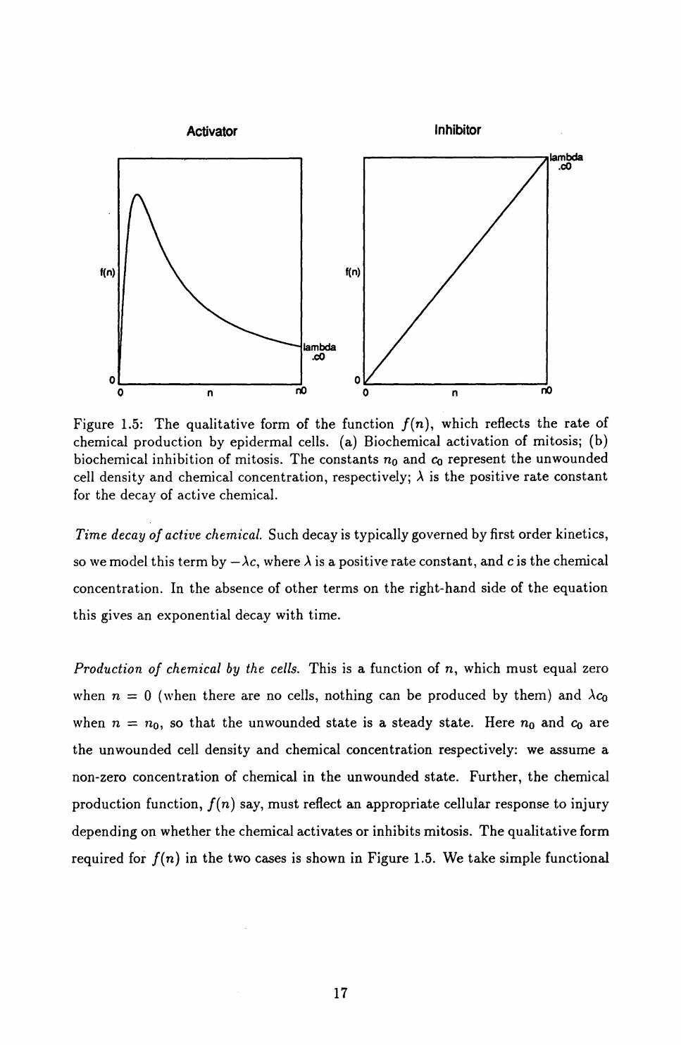
Figure 1.5: The qualitative form of the function /(n), which reflects the rate of chemical production by epidermal cells, (a) Biochemical activation of mitosis; (b) biochemical inhibition of mitosis. The constants no and CQ represent the unwounded cell density and chemical concentration, respectively; A is the positive rate constant for the decay of active chemical.

Time decay of active chemical. Such decay is typically governed by first order kinetics,

so we model this term by Ac, where A is a positive rate constant, and c is the chemical

concentration. In the absence of other terms on the right-hand side of the equation

this gives an exponential decay with time.

Production of chemical by the cells. This is a function of n, which must equal zero

when n — 0 (when there are no cells, nothing can be produced by them) and \CQ

when n = ?IQ, so that the unwounded state is a steady state. Here n0 and CQ are

the unwounded cell density and chemical concentration respectively: we assume a

non-zero concentration of chemical in the unwounded state. Further, the chemical

production function, f(n) say, must reflect an appropriate cellular response to injury

depending on whether the chemical activates or inhibits mitosis. The qualitative form

required for f(n) in the two cases is shown in Figure 1.5. We take simple functional

17

forms that satisfy these requirements, namely

n/(n) = Aco • — • I -?——r 1 for the activator••» > «2 "2 I

and f(n) = —— • n for the inhibitor,no

where a is a positive constant which relates to the maximum rate of chemical pro­

duction.

Rate of natural cell loss. This is due to the sloughing of the outermost layer of

epidermal cells, and we take it as proportional to n, say kn, where A: is a positive

constant.

Chemically controlled cell division. We choose this term so that when c = CQ, the

unwounded chemical concentration, the net reaction term in the cell conservation

equation is of logistic growth form, kn(l — n/n0 ); here k is the linear mitotic rate.

Thus we take the rate of cell division as s(c) • n • (2 — n/n0 ), where s(c) reflects the

chemical control of mitosis, and S(CQ) = k . The qualitative form required for s(c) is

shown in Figure 1.6. In the case of a chemical activator, a decrease of s(c) to s(Q) for

large c is included because it is found experimentally in vitro (Eisinger et a/., 1988a);

however, one prediction of the model is that this phenomenon has little effect in vivo.

For both types of regulation we require 0 < s(oo) < smax = hk, say, where h is a

positive constant, and we take 5(00) = &/2; the model solutions are not sensitive to

variations in s(oo). Again we take simple functional forms satisfying these criteria,

namely(h-l)c+hcosc = k •

for the inhibitor, and

for the activator. Here cm (> CQ) is the value of c giving the maximum level of

chemical activation of mitosis.

18

Activator Inhibitor

s(c)

0 CO

Figure 1.6: The qualitative form of the function s(c), which reflects the chemical control of mitosis, (a) Biochemical activation of mitosis; (b) biochemical inhibition of mitosis. The constant CQ represents the chemical concentration in the unwounded steady state, and the parameter k is equal to the reciprocal of the cell cycle time.

Thus the model system is

Ot

fir~

(2 - — - knUQ)

with initial conditions n = c = 0 inside the wound domain and boundary conditions

n = HQ and c = CQ on the wound boundary, at all times t. To clarify the roles of the

various parameters, we nondimensionalize the model using a length scale L (a typical

linear dimension of the wound) and time scale l/k (the cell cycle time seems the most

relevant time scale). We define the following dimensionless quantities, denoted by *:

n* = n/n0 c" = C/CQ r * = r/L t* = kt

= /(n0 - n s m (cm ) = s(co - cm )/k D* = D/(kL2 )

= Dc/(kL2 ) \* = \/k c*m = a' = a/no.

For the circular wounds considered below, we take L to be the initial wound radius.

In the remainder of this chapter and Chapter 2, we drop the asterisks for notational

19

simplicity, and use the superscript dim to denote the dimensional value correspond­ ing to a dimensionless parameter. With these rescalings, the dimensionless model equations are

dn = D V2n\JL

flr^ = £cV2 c at

with initial conditions n = c = 0 inside the wound domain and boundary conditions n = c = 1 on the wound boundary, at all times t. Here, for the activator kinetics

where ?=n2 -f a2I I V

and for the inhibitor kinetics

/(n) = n, s(c) =

where we assume h > 1 and cm > 1.

1.4 Linear Analysis and Parameter ValuesA biological requirement of the model (1.6) is that the unwounded state is stable to small perturbations in cell density and chemical concentration, while the wounded state is unstable. This imposes various conditions on the model parameters, which we now derive by linearizing about these steady states. Consider first the unwounded state, n = c = 1, which is a steady state since s(l) = /(I) = 1. Linearizing about this gives

r\

(1.7b)

where HI = n — l and c\ = c— 1, with |ni|, |ci| <£ 1. We look for plane wave solutions, ni = fi 1 el^-~u/*J, GI = de*^-""*), where K_ is the wave vector and fi 1? ci and u; are constants. Since the equations (1.7) are linear, any solution can be written as a sum

20

of such plane wave solutions. Substituting these forms into (1.7) gives

(A + DC K2 - i

where K = |/JC|. Thus for non-trivial solutions we require

(1 + DK2 - tw)(A + DCK2 - iu) = A/'

a quadratic dispersion relation for w(K). For stability to small perturbations it is

necessary and sufficient that Im(u;) < 0 for all K. By solving the quadratic, this

occurs if and only if for all K > 0,

1 + A + (D + DC )K2 > 0

and

The first of these inequalities holds since A, D and Dc are positive, and the second is

satisfied since in both the activator and inhibitor cases, /'(I) and s'(l) have opposite

signs. Thus the stability requirement for the unwounded state imposes no constraints

on the parameter values.

Linearizing about the wounded steady state n = c = 0 and looking for plane wave

solutions in the same way gives the dispersion relation

(DK* - iw - 2^(0) + 1)(DCK2 - iw + A) = 0.

We assume that any perturbation involves all wave numbers K. This is a standard

assumption in biological contexts (see, for example, Murray, 1989), and is justified

because of a degree of stochasticity in all biological systems. For instability, one of the

two roots for u must therefore have a positive imaginary part for some K. But Dc and

A are positive so we require that, for some K, DK2 — 2.s(0) + l < 0, that is ,s(0) > 1/2.

For the activator kinetics, this condition is cm > (1h — 1) + J(1h — I) 2 — 1, and for

the inhibitor kinetics, it is simply h > 1/2.

It is possible to estimate the parameters A, h and k from experimental data.

We estimate A in the case of a chemical inhibitor using data on chalones. Brugal

21

and Pelmont (1975) found a decrease in the proliferation rate in intestinal epithelium

during the 12 hours after injection with epithelial extract. Also Hennings et al. (1969)

were able to maintain suppression of epidermal DNA synthesis by repeated injection

of epidermal extract at 12 hour intervals. Based on these studies, we take the half-life

of chemical decay as 12 hours. If we consider only the decay term in equation (1.5b),

this gives exponential decay with a dimensional half-life of (Iog2)/Adim . We therefore

take Adim = 0.05 (w ^Iog2)h~1 .

In the case of a chemical activator, there is little quantitative experimental data.

However, comparison of the work of Eisinger et al. (1988a,b) on the role of chemical

activators in wound healing with the clinical studies of chalone effects by Rytomaa

and Kiviniemi (1969, 1970) suggests a longer time scale for the chalone activity, by

a factor of about 6, so we take Adim = 0.3 h"1 for the activator.

The. parameter k is simply the reciprocal of the epidermal cell cycle time. This

varies from species to species, but is typically about 100 hours (Wright, 1983), so we

take k = 0.01 h" 1 . The value of h is the maximum factor by which the mitotic rate

can increase as a result of chemical regulation. We take h — 10, since this factor is

suggested both by a study of epidermal wound healing in pigs (Winter, 1972) and by

experiments on corneal wound healing in rabbits (Danjo et a/., 1987). The values of

the diffusion coefficients D and Dc were estimated by comparing the model solutions

with experimental data on wound healing, as discussed below, since there is at present

no direct experimental data from which they can be determined.

In the activator case, the parameters ot and cm have to be chosen so that the func­

tions f(n) and s(c) have appropriate qualitative forms. The linear analysis imposes

the constraint cm > 37.97 when h = 10, and we take cm = 40 and a = 0.1.

1.5 Numerical Solution of the Improved ModelWe solved the system of reaction-diffusion equations (1.6) numerically in a radi­

ally symmetric cylindrical geometry, using the method of lines on a uniform space

mesh, and solving the resulting system of ordinary differential equations using Gear's

22

Wound Radiuso

"fe

i «

CD Van d«n Br«nk (1956)O Van d*n Br«nk (1956)A Crosson «t al. (1966)Z Lindquist (1946)O Zlcsk* «t al. (1987)O Zi«sk« tt al. (1987)X fronts «t al. (1989)

«£> "^

a

20 40 80 100 Time /%

Figure 1.7: Comparison of data from a number of quantitative studies on the healing of circular epidermal wounds. The sources of the data are as indicated in the key. In Lindquist's (1946) experiments there is some dermal contraction, and we have extrapolated to the case of no contraction. These studies involve a range of species and wounding locations, and the speed of healing varies by almost an order of magnitude. However, when time is expressed as a percentage of total healing time, as here, the agreement between the different data sets is remarkable.

method, as in Section 1.2.

As explained above, determination of the diffusion coefficients D and Dc requires

comparison of the model solutions with data from quantitative studies of epidermal

wound healing. There are a number of such studies, and almost all involve circular

wounds. The speed of healing differs widely between species and wounding location,

almost by an order of magnitude. However, when time is expressed as a fraction

of total healing time, the agreement between different sets of data is remarkable

(Figure 1.7). As discussed in Section 1.2, the key aspect of this data is the biphasic

nature of the healing process: a lag phase followed by a linear phase. Given that we

are basing the values of parameters in the reaction terms on experiments spanning a

range of species and cell locations, we felt it inappropriate to select one set of data

and to then choose the diffusion coefficients D and Dc by fitting the model solution

to both the form and precise time course of this data. Rather, we fit the model

solution to the data as illustrated in Figure 1.7, with time expressed as a fraction

23

of total healing time. Of course we look for the model to predict wound speeds of

the observed order of magnitude, but more exact quantitative prediction of both the

form and speed of healing will require data from the particular species and wound

location, from which the parameters in the reaction terms can be estimated.

The results of this approach are illustrated in Figure 1.8, which shows the numer­

ically calculated decrease in wound radius with time for the two sets of kinetics. As

in Section 1.2, we capture the concept of 'wound radius' from our model by taking

the wound as 'healed' when the cell density reaches 80% of its unwounded level, that

is when n = 0.8 for the dimensionless equations. The choice of this critical level

as 80% is somewhat arbitrary, but does not significantly affect the results since the

solutions for n and c are of travelling wave form, as discussed below. For clarity, in

Figure 1.8 we have compared this predicted variation in wound radius to the data of

only one of the authors discussed above. The dimensional diffusion coefficients giving

this healing profile are D = 4 x lO'^cn^s" 1 , Dc = 3 x 10~7cm2s~ 1 for the activator

kinetics, and D = 7 x 10~ 11 cm2s~ 1 , Dc = 6 x 10~6 cm2s~ 1 for the inhibitor kinetics.

These are biologically reasonable for cells and biochemicals of moderate molecular

weight, respectively. In Figure 1.8 we also plot the cell density n and chemical con­

centration c as a function of the radius r at a selection of equally spaced times. As

expected intuitively, the form of the solutions is of a front of epidermal cells moving

into the wound, with an associated wave of chemical. For a wound of radius 0.5cm,

the speed of these fronts in the 'linear phase' of healing corresponds to dimensional

wave speeds of 2.6//m hr" 1 for the activator and 1.2//m hr" 1 for the inhibitor, which

are of the experimentally observed order of magnitude.

Since the exact form of the initial conditions is somewhat arbitrary, we investi­

gated the stability of the linear phase solution forms to perturbations in the initial

conditions. The initial values at r = 1 were maintained at n = c = 1, and a variety of

initial values for n and c were assigned to the adjacent space nodes. For both types of

chemical, the solution form was found to be stable to these perturbations: the wave

form quickly settled down to that shown in Figure 1.8.

We should stress that the agreement between data sets illustrated in Figure 1.7

24

n(r,t) at equally-spaced times Wound Radius (-) Compared to Data (1,2)Wound Radius

0.0 0.4 0.6 0.8 1.0r

40 60 80 100Time / %

c(r,t) at equally-spaced times

PARAMETER VALUES

D = 5e-4

DC = 0.45

Cm= 40

Alpha= 0.1

Lambda = 30

h= 10

Figure 1.8: (a) Numerical solutions of equation (1.6) in a radially symmetric ge­ ometry for the activator kinetics. Cell density n and chemical concentration c are plotted against radius r at a selection of equally spaced times. We also show the corresponding decrease in wound radius with time, expressed as a percentage of total healing time, and compare this to experimental data from Van den Brenk (1956). The dimensionless parameter values are as indicated.

25

n(r,t) at equally-spaced times Wound Radius (-) Compared to Data (1,2)Wound Radius

0.0 0.2 0.4 0.6 0.8 1.0 40 60 80 100Time / %

c(r,t) at equally-spaced times

CM

O OJ

q 6

PARAMETER VALUES

D= 1e-4

Oc = 0.85

Lambda^ 5

h= 10

o.o 0.2 0.4

r

0.6

I

0.8 1.0r

Figure 1.8: (b) Numerical solutions of equation (1.6) in a radially symmetric ge­ ometry for the inhibitor kinetics. Cell density n and chemical concentration c are plotted against radius r at a selection of equally spaced times. We also show the corresponding decrease in wound radius with time, expressed as a percentage of total healing time, and compare this to experimental data from Van den Brenk (1956). The dimensionless parameter values are as indicated.

26

does depend crucially on all the wounds having roughly the same initial size. It

is clear intuitively that for a large wound, the lag phase will represent a smaller

fraction of the total healing time, and vice versa. This phenomenon is reflected in

the model solutions, since as the wound radius R increases, the dimensionless diffusion

coefficients decrease in proportion to l/R2 .

1.6 Travelling Wave SolutionsFor both types of chemical, the qualitative form of the solution in the 'linear phase'

of healing is of waves of cells and chemical moving into the wound with constant

shape and constant speed. Such a solution is amenable to analysis if we consider a

one-dimensional geometry, rather than the two-dimensional radially symmetric ge­

ometry of Section 1.5. This is biologically relevant for large wounds of any shape,

since to a good approximation these are one-dimensional during much of the healing

process. Numerical solutions of the model equations for this new geometry are shown

in Figure 1.9; there are no significant differences between these solutions and those of

the two-dimensional system illustrated in Figure 1.8. The dimensionless wave speeds

in this case are about 0.05 for the activator and 0.03 for the inhibitor.

Mathematically, solutions of constant shape and speed are travelling waves, that

is, solutions of the form n(x,t) = N(z), c(x,t) = C(z), z = x -f at, where x is the

spatial coordinate and a is the wave speed, positive since we consider waves that

are moving to the left. Substituting these solution forms into the reaction-diffusion

system (1.6) gives the ordinary differential equations

aN1 = QN" + s(C)'N.(2-N)-N

aC' = DC C" + \f(N) - AC , (l.Sb)

where prime denotes d/dz. Equation (1.6) holds on a finite space domain and a

semi-infinite time domain, which does not correspond to a well-defined z domain.

However, during the majority of the 'linear phase' of healing, numerical solutions of

(1.6) have n,c « 0 near the centre of the wound and n,c % 1 near the wound edge,

27

n(x,t) for activator c(x,t) for activatoro«

9 -

q ci

s J

o d T

o.o

n(x,t) for inhibitor

0.2 0.4 0.6 0.8

c(x,t) for inhibitor

1.0X

*CM

O CV

to o

oO

0.0

I

0.2

T

0.4

I

0.6

I

0.8 1.0 X

Figure 1.9: Numerical solutions of equation (1.6) in a one-dimensional geometry, for both chemical activation and chemical inhibition of mitosis. Cell density n and chemical concentration c are plotted as a function of the spatial coordinate x at a selection of equally spaced times. The dimensionless wound domain is — 1 < x < 1. The parameter values are as in Figure 1.8.

28

and differ from these steady state values only in a localized region. The wave form

can therefore be reasonably represented by solving (1.8) on — oo < z < oo, with

boundary conditions N(-oo) = C(-oo) = 0 and N(+oo) = £(+00) = 1.

In the remainder of this chapter, we investigate these travelling wave forms. In

particular, since the system of ordinary differential equations is fourth order and

thus difficult to analyse globally, we consider two approximations which reduce the

order of the system: firstly treating A as infinite and secondly treating D as zero.

Biologically, the first approximation corresponds to active chemical decaying as it

is produced, and the second corresponds to an absence of cellular diffusion, so that

changes in cell density are due only to mitosis.

In the case of the activator kinetics, recall that

1cm (h-(3)c , Q c2m - 1hcm + 1

But c < cm for all x and t (Figure 1.9), and thus it is a good approximation to

take s(c) as simply a linear function. Specifically, we approximate <?m -f c2 w (?m and

ft « (cm - 2/i)/(cm - 2), which give s(c) ss 70 + 1 - 7 where 7 = 2(h - l)/(cm - 2).

Numerical solutions of the model equations (1.6) using this form differ negligibly

from those with the original s(c) in both the one-dimensional and radially symmetric

two-dimensional geometries. We use this linear approximation in the subsequent

analysis, since it makes this analysis much easier algebraically. The approximation is

valid provided cm ^> 1.

1.6.1 Solutions with A = ooIn the first approximation we consider the derivative terms in the second equation

to be negligible compared to the reaction terms. Intuitively this seems a reasonable

approximation in the case of the inhibitor mechanism (A = 5), and a good approxima­

tion for the activator kinetics (A = 30). The fourth order system (1.8) then reduces to

a second order ordinary differential equation for TV, which can be analysed relatively

29

easily. Specifically, we have

i(1.9)

where $(N) = s[f(N)]-(2N-N2)-N. We look for a solution subject to 7V(+oo) = 1

and N(— co) = 0, with TV > 0 for all z. Straightforward algebra gives the functional

form oi ^(N) as

(cm -- 1) +a2 (6h -cm - 4)]N + a2 (2 - 4fc + cm )} (l.lOa)

for the activator, and

for the inhibitor. These are shown graphically in Figure 1.10 for the parameter values

used in Figure 1.8. Crucially, on the interval [0, 1] both functions have an essentially

parabolic shape. Thus we expect much of the standard analysis for travelling wave

solutions of the Fisher equation ut = uxx + u(l — u) to be applicable here, albeit with

more complicated algebra. This standard analysis is described in detail by Murray

(1989).

The system (1.9) has singular points N = Nf = 0 and TV = 1, TV' = 0. At (0,0) the

eigenvalues are [a ± {a2 + 4D - SDs (O)} 1 /2 ] /ID. Now the linear analysis presented

in Section 1.4 implies that 5(0) > 1/2. Thus (0,0) is an unstable node or unstable

focus according to the sign of [a 2 + 4Z> - SDs(Q)]. Since we require N non- negative,

we have a condition on the wave speed for a solution of the required form to exist,

namely a > amin = 2{£>(2s(0) - I)} 1 / 2 .

For (1,0) the eigenvalues are [a ± {a2 + 4D - 4As/ (l)// (l)} 1 /2] /2D. In both the

activator and inhibitor cases $'(1) and /'(I) have opposite signs, so that this equilib­

rium is a saddle point.*

For both fixed points, the eigenvector corresponding to an eigenvalue // is (1, /*).

Therefore, provided a > amtn , the phase portrait has the form shown in Figure 1.11.

Thus there is a unique solution of the required form for each a > amm, corresponding

30

psio

psi(N) for activator psi(N) for activator near originpsi

3 J

pO

in

CM jT -

-1.0

I

-0.5

I

0.0

I

0.5 1.0 1.5

N

T

-6 -2 080

2 0-4

4e-4 N

psi(N) for inhibitor

-1.0

Figure 1.10: The function *{>(N), defined in (1.10), for the activator and inhibitor kinetics. A more detailed plot near the origin is shown in the activator case. The parameter values are as in Figure 1.8.

31

A/'

Figure 1.11: The qualitative form of the phase portrait for (1.9) with a > amin - The dashed trajectory corresponds to the unique solution satisfying N(+oo) = 1, N(-oo) = 0 and TV > 0.

to the dashed trajectory in Figure 1.11. However, Kolmogoroff et al. (1937) showed that for a class of one-dimensional reaction-diffusion equations that includes (1.6) when A = oo, as t increases the solution approaches the travelling wave form with a = a-min when the initial conditions have compact support, that is n = 1 for sufficiently large positive x, and n = 0 for sufficiently large negative x. (A simplified translation of the paper of Kolmogoroff et al. (1937) is given in Oliveira-Pinto and Conolly, 1982, Chapter 7). For the parameter values we are using, amtn is about is 0.01 for the activator and 0.09 for the inhibitor. These values compare to the wave speeds 0.05 and 0.03 respectively found in the one-dimensional numerical solutions of the partial differential equation system (1.6). The discrepancy indicates inadequacies in the approximation of chemical decaying as it is formed; intuitively, we expect this approximation to give a lower wave speed for the activator kinetics and a higher wave speed for the inhibitor kinetics.

Rescaling the independent variable in the Fisher equation (znew = z0id/a) gives tu" — u' -f u(l — u) = 0, where e = a~2 . This enables the equations to be solved analytically as a regular perturbation problem in the small parameter e (see, for example, Murray, 1989). A corresponding rescaling for (1.9) gives

= 0 (1.11)

where c. = D/a2 and prime denotes d/d(, C = z/a. Therefore a solution can be

32

obtained in the same way for the inhibitor kinetics (D/a?min w 0.01), but not for the

activator kinetics (D/a^in w 5). We look for a solution of the form

Substituting this into (1.11) and equating coefficients of powers of e gives

f, -dN0

subject to A^o(-oo) = 0, 7V0 (0) = 1/2, #0(+oo) = 1, and A^-oo) = 7V;(0) =

Ni(+oo) = 0 for i > 1. The value of A^(0) is arbitrary; it must be specified to give a

unique solution. Since we choose N(Q) = 1/2,

-1:..„,., ln[2JV0]-

'Ih-lln[2(l-7V0 )]

- 2) In (1.13)

for the inhibitor kinetics, using (l.lOb). This cannot be inverted explicitly. However,

observing that £ is a rnonotonically increasing function of NO when h > 1, we take

TVo, rather than £, as the independent variable. Dividing (1.12b) by dNo/d( gives

dN0di/>(N0 )

o) dN0 dN0 '

using (1.12a). Dividing through by ^(N0 ) gives

= 0.

Thus, since 7V\ = 0 when N0 = 1/2 (at C = 0),

(1.14)

33

n(z), n(r,t)

CM

oq d

to d

CNJ d

q d

0.5

Figure 1.12: Comparison of 7V0 (full curve), NO 4- cNi (small dots) and the numerical solution of the partial differential equations (1.6) at a time in the middle of the 'linear phase' of healing (curve and large dots) for the inhibitor kinetics. Here NO and N\ are the first two terms in the asymptotic expansion of N(z), given in (1.13) and (1.14) respectively. The parameter values are as in Figure 1.8, with a = amtn w 0.09. The 0(e) correction to No is barely visible.

34

Plots of NQ and N0 + tNi against z are shown in Figure 1.12 and compared to the

numerical solution of the partial differential equations (1.6) at a time in the middle

of the 'linear phase' of healing. These show that the first order correction cNi is

already very small. The agreement between the partial differential equation solution

and the travelling wave form is poor. In particular, the travelling wave solution fails

to capture the important feature that n > 1 in part of the wave front. This is an

inadequacy in the approximation A = oo.

Numerical solutions of (1.9) for the activator kinetics with a = amin show a similar

poor agreement with the partial differential equation wave form. As explained on

page 33, the perturbation theory method of solution that we have used is invalid

in this case since Z)/a^t-n w 5. However, the method can be used for both types

of kinetics if we take a as the wave speed observed in the numerical solution of

the partial differential equations. This gives D/a2 as 0.2 for the activator kinetics

and D/a 2 w 0.1 for the inhibitor kinetics. For the activator, analytic evaluation

of the integral for z(No) is algebraically infeasible, and we evaluated it numerically

using Gauss-Legendre quadrature. For the inhibitor mechanism, the analytic solution

above is still valid for this new wave speed. Again, the solutions thus obtained do

not compare well with the partial differential equation wave forms, and again this

is an inadequacy in the approximation A = oo rather than in the truncation of the

asymptotic expansion.

1.6.2 Solutions with D = 0Given the shortcomings of the approximation investigated in the previous section, we

now consider the approximation D = 0. Recall that in Section 1.5 we determined

the values D = 5 x 10~ 4 for the activator kinetics and D = 10~4 for the inhibitor

kinetics, by fitting to experimental data. Putting D = 0, the fourth order system

(1.8) reduces to a third order system

N' = -— + -s(C)(2N-N2 ) (1.15a) a a

c" = + "-M- < uab >

35

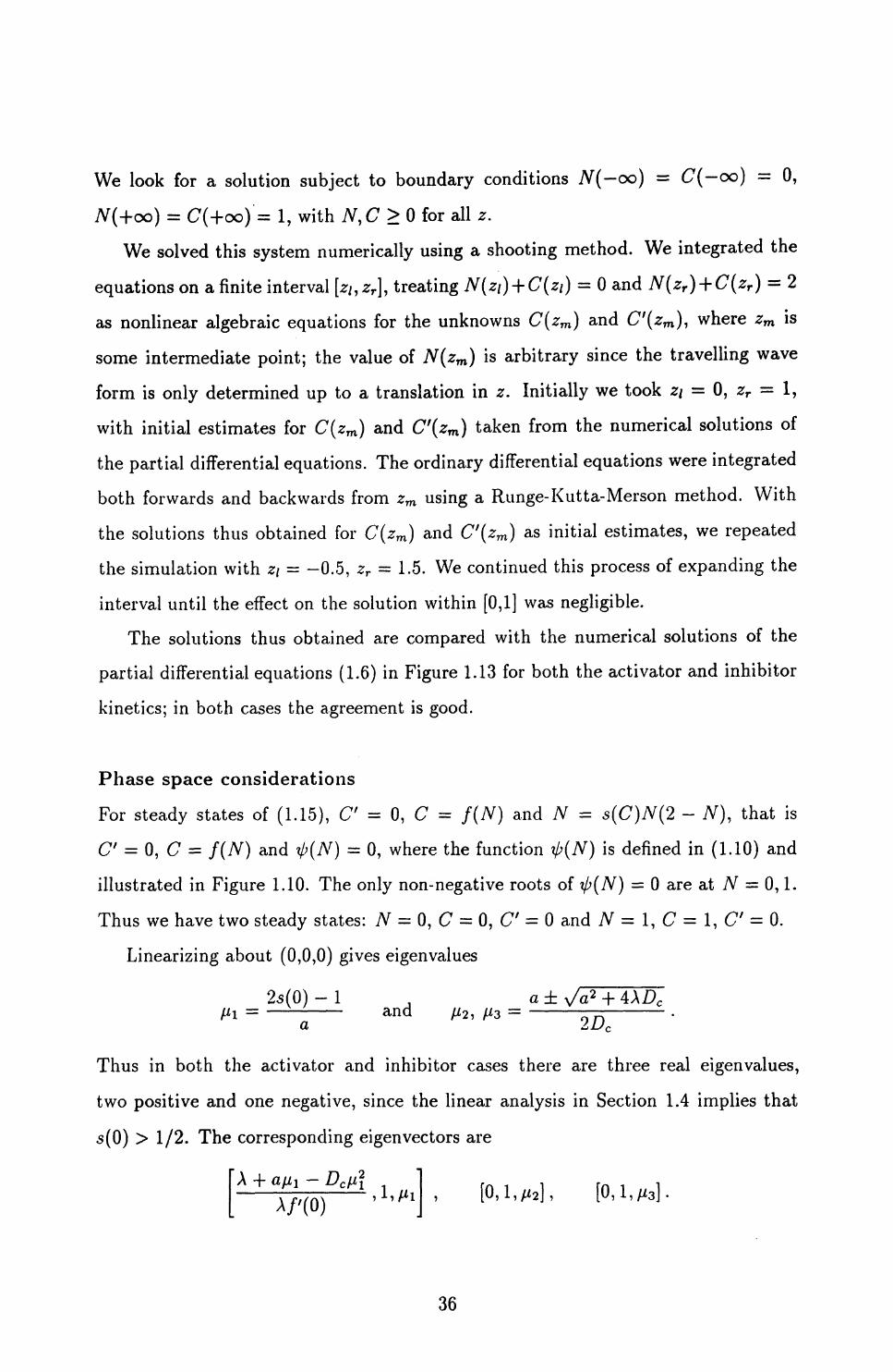
We look for a solution subject to boundary conditions N(—oo) = C(—oo) = 0,

Af(+oo) = C(+oo) = 1, with N,C > 0 for all z.

We solved this system numerically using a shooting method. We integrated the

equations on a finite interval [z^ zr], treating N(zi) + C(z{) = 0 and N(zr ) + C(zT ) = 2

as nonlinear algebraic equations for the unknowns C(zm ) and C'(zm ), where zm is

some intermediate point; the value of N(zm ) is arbitrary since the travelling wave

form is only determined up to a translation in z. Initially we took z\ — 0, zr = 1,

with initial estimates for C(zm ) and C'(zm ) taken from the numerical solutions of

the partial differential equations. The ordinary differential equations were integrated

both forwards and backwards from zm using a Runge-Kutta-Merson method. With

the solutions thus obtained for C(zm ) and C'(zm ) as initial estimates, we repeated

the simulation with z\ = -0.5, zr = 1.5. We continued this process of expanding the

interval until the effect on the solution within [0,1] was negligible.

The solutions thus obtained are compared with the numerical solutions of the

partial differential equations (1.6) in Figure 1.13 for both the activator and inhibitor

kinetics; in both cases the agreement is good.

Phase space considerations

For steady states of (1.15), C' = 0, C = f(N) and TV = s(C)N(2 - N), that is

C' = 0, C = f(N) and ij>(N) = 0, where the function </>(7V) is defined in (1.10) and

illustrated in Figure 1.10. The only non-negative roots of ij>(N) = 0 are at TV = 0,1.

Thus we have two steady states: N = 0, C = 0, C' = 0 and N = 1, C = 1, C' = 0.

Linearizing about (0,0,0) gives eigenvalues

25(0)-1 . a ± Va2 + 4Ar a ™ r ° Wc

Thus in both the activator and inhibitor cases there are three real eigenvalues,

two positive and one negative, since the linear analysis in Section 1.4 implies that

> 1/2. The corresponding eigenvectors are'A +

36

N(z),n(r,t)Activator

C(z),c(r,t)Activator

o m

S

CMd

o d

in d

od

0.0 0.2 0.4 0.6 0.8 1.0z, r

N(z), n(r,t)CM

Inhibitor

0.0 0.2 0.4 0.6

Inhibitor

0.8 1.0z, r

to d

CMd

C(z),c(r,t)p _ •——

<Dd

CMd

o d

0.0 0.2 0.4 0.6 0.8 1.0z,r 0.0 0.2

I

0.4 0.6 0.8 1.0z, r

Figure 1.13: Comparison of numerical solutions of the full model equations (1.6) in one space dimension (full curves) and the travelling wave equations under the approximation D = 0, given in (1.15) (dotted curves). The parameter values are as in Figure 1.8, with a = 0.05 for the activator and a = 0.03 for the inhibitor. These are the dimensionless wave speeds observed in the one-dimensional solutions of (1.6).

37

For (1,1,0) the eigenvalues are the roots of

0 ' (U6)which is plotted in Figure 1.14 for both the activator and inhibitor kinetics, for a

range of wave speeds around that observed in the numerical solution of the one-

dimensional partial differential equations. In the inhibitor case there are three real

eigenvalues, two negative and one positive; in the activator case either this is also the

case or there is one real positive and two complex eigenvalues, depending upon the

wave speed.

For this steady state, analytic determination of the eigenvalues and eigenvectors is

algebraically unfeasible, so we determined them numerically. The results are shown

in Tables 4.1 and 4,2, again for both types of chemical and for a range of wave

speeds around those found in the numerical solutions of the one-dimensional partial

differential equations.

For the activator kinetics, these considerations imply an upper bound on the

wave speed a. This is because we look for a solution with a monotonic rather than

oscillatory approach to the un wounded steady state (1,1,0). Thus our upper bound

is the value of a at which (1.16) has two equal negative roots. We write this cubic as

p(x] = x3 + ax2 — fix — 7, where a and 7 depend on a. If p(x) = p'(x) = 0 for some

#, then

x{9~f-a/3}{(3x + a)p'(x)-9p(x)} = {2a2

If x ^ 0, this simplifies to

a2 /?2 + 4/?3 + 18a/?7 - 2772 + 4a37 = 0 . (1.17)

Now

7 = a \ Dc • •' '

substituting these into (1.17) and multiplying through by a4 gives a cubic in a2 ,

38

Activatorcubic cubic

Activator near origin

-100 -80 -60 -40 -20 0 20 40 60eigenvalue

T

-20

I

-10 10 20eigenvalue

cubic Inhibitorcubic

Inhibitor near origin

-150

r -100 -50

I

0

8o

o

50 100 150eigenvalue-10 5 10 •

eigenvalue

Figure 1.14: The left-hand side of the cubic eigenvalue equation (1.16), plotted against A, in the activator and inhibitor cases, for 5 values of the wave speed a, which are 0.01, 0.03, 0.05, 0.07, 0.11 for the activator, and 0.01, 0.025, 0.035, 0.05, 0.1 for the inhibitor. The wave speeds observed in the numerical solution of the one-dimensional partial differential equations are about 0.05 for the activator and 0.03 for the inhibitor. The intercept on the vertical axis becomes less negative as the wave speed increases.

39

Speed, a0.038

0.048

0.058

Eigenvalues-24.84

9.50-10.89-11.65

9.43-18.51

9.38•13.24 ±

2.02t

Corresponding eigenvectors(0.322,0.038,-0.946) (0.036,0.105, 0.994) (0.074,O.Q91,-0.993)(0.092,0.085,-0.992) (0.034,0.105, 0.994) (0.224,0.053,-0.973)(0.033,0.106,0.994)(-0.128 ±0.042t,- 0.073 TO.Olli, 0.988)

Table 1.1: Eigenvalues and eigenvectors of equations (1.15) at the steady state (1,1,0), for the activator kinetics, for three values of the wave speed a. The other parameter values are as in Figure 1.8.

Speed, a0.0204

0.0304

0.0404

Eigenvalues-48.96 -2.96 2.93

-32.81 -2.97 2.92

-24.64 -2.98 2.92

Corresponding eigenvectors(0.993,-0.002, 0.120) (0.159,-0.316, 0.935) (0.143,-0.320,-0.937)(0.984,-0.005,0.177) (0.164,-0.314, 0.935) (0.139,-0.321,-0.937)(0.972,-0.009, 0.234) (0.169,-0.313, 0.935) (0.136,-0.321, 0.937)

Table 1.2: Eigenvalues and eigenvectors of equations (1.15) at the steady state (1,1,0), for the activator kinetics, for three values of the wave speed a. The other parameter values are as in Figure 1.8.

40

cubic

I

-0.2 •0.1

I

0.0

cubic 8

o.i a*a 0.00290 0.00295 0.00300 0.00305 0.00310a*a

Figure 1.15: The cubic equation (1.18) for a^ax , with a more detailed plot near the biologically relevant root.

{[(1 + A) 2 - 4r]/4A;}a6 + {4F(3 + £>') - 18(1 + A)F + 2(1 + A) 2 (l + 2A)}a4

+ DC {(1 + A) 2 + 3F(6A + 2 - 9F)}a2 + = 0 . (1.18)

This is plotted in Figure 1.15 for the parameter values we are using. There is a unique

solution in (0.0,0.1), which must therefore be aj^, where amax is the upper bound.

Solving the cubic numerically gives amax w 0.0546, which is close to the wave speed

of about 0.05 observed for the activator mechanism in the numerical solutions of the

partial differential equations (1.6) in one space dimension.

Perturbation analysis for the activator mechanism

For the activator kinetics, we can obtain an analytic approximation to the travelling

wave form with D = 0 using regular perturbation theory. We rewrite (1.15) as

aJV4 = e(C - l)(2N - TV 2 ) + (TV - N2 )

DcC"-aC'-\C = -A-

41

and treat c = 2(h - l)/(cm - 2) w 0.47 as a small parameter. With this value for

e, we will require the 0(e) correction to the 0(1) solution. The boundary conditions

remain N(-oo) = C(-oo) = 0 and A^(+oo) = <7(+oo) = 1, with N(Q) = 1/2 for

uniqueness. We look for a solution of the form

N(z-c) = N0 (z) + eNl (z) + e2 N2 (z) + ." (1.20a)

= C0 (z) + eCi(z) + <?C2 (z) + • • • . (1.20b)

Substituting this into (1.19) and equating coefficients of e° gives

aN0 = No-N*"

Changing the independent variable to £ = e*/a , these become

(1.21)

where AC = a~ 2 Dc and prime denotes d/d£. The relevant boundary conditions are

7V0 (+oo) = Co(-foo) = 1, N0 (Q) = C0 (0) = 0 and N0 (l) = 1/2. Straightforward

separation of variables gives NO = £/(! + £). The equation for Co can then be solved

using the method of undetermined coefficients. The corresponding homogeneous

equation has linearly independent solutions y oc £9 , where

(1.22)

Therefore we look for a solution of the form Co = 7+(<0£9+ + 7-(£)£9 ~ subject to

the constraint 7+<f9 +7l£<r = 0. Substituting this into (1.21) gives linear equations

for 7±, whose solution is

f = 7± ' '

42

Therefore

A(l+a2 )4A/c

P-f OO

/*Jo ud

N0 (u)

4-

du10 ww+i) 7Vo(w) 2 + a2

Here the values of the constant limits are necessary (but not sufficient) for convergence

at ( = 0 and +00 respectively.

We consider the boundary conditions, which imply convergence, by investigating

the behaviour of each of the two integrals in (1.23) as ( approaches 0 and +00. We

have

limf -lU-fr

r+oo 1 N0 (u) dua

= lim

= lim

1 /-+00 111/6

du

using L'Hopital's rule and the expression for NQ. Similarly

Hm r r -^t-++oo Jo u(V

N0 (u) -1——- du = —

Thus

Co(-foo) =4A/c

J___Li"^" n~

= 1

using (1.22). Similarly the condition at £ = 0 is satisfied.

We now consider the first order perturbations. Equating coefficients of e 1 in the

original ordinary differential equations (1.19) gives

(1.24a)

(1.24b)= -A(l+a2 )a2 -

43

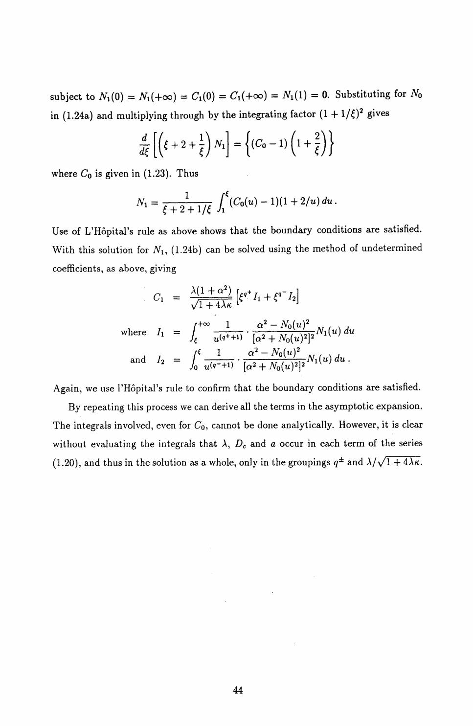
subject to Ni(Q) = JVi(-foo) = Ci(0) = Ci(+oc) = Ni(l) = 0. Substituting for N0

in (1.24a) and multiplying through by the integrating factor (1 + l/£)2 gives

t.where C0 is given in (1.23). Thus

1

= {(C0 -

2/u) du .

Use of L'Hopital's rule as above shows that the boundary conditions are satisfied.

With this solution for A/i, (1.24b) can be solved using the method of undetermined

coefficients, as above, giving

.. ( . ,where /i = / - v NI(U) du

+ [a2 + A/•

= Jo

•« 1[a* +

Again, we use I'Hopital's rule to confirm that the boundary conditions are satisfied.

By repeating this process we can derive all the terms in the asymptotic expansion.

The integrals involved, even for Co, cannot be done analytically. However, it is clear

without evaluating the integrals that A, Dc and a occur in each term of the series

(1.20), and thus in the solution as a whole, only in the groupings g± and A/\/l 4- 4A/c.

44

Chapter 2

Mathematical Experiments and Implications for Wound Geometry

2.1 Addition of ChemicalsIn Chapter 1 we constructed a mathematical model for epidermal wound healing. The

parameter values are based as far as possible on experimental data, and solutions of

the model with either chemical activation or inhibition of mitosis compare well with

experimental data on the normal healing of circular wounds. In this chapter, we use

this model to perform various 'mathematical experiments', which will enable us to

make clinically testable predictions.

The model (1.6) is based on chemical auto-regulation of cell division, and we begin

by investigating the effect of putting additional quantities of the mitosis-regulating

chemical onto the wound surface. Such a procedure is feasible experimentally, since

some growth factors are available in isolated forms. Moreover, cell extracts and

exudates have also been successfully added to wounds in vivo (Yamaguchi et a/., 1974;

Eisinger et a/., 19S8a; Madden et a/., 1989). To simulate such an addition of chemical,

we solved the model equations in a two-dimensional radially symmetric geometry, as

in Section 1.5, but when the wound area had decreased to half of its initial value, we

increased the dimensionless chemical concentration by cadd at all points within the

wound area. Here the 'wound area' is defined by the condition n < 0.8, as discussed

on page 24. The effects of this single addition of mitosis-regulating chemical on the

healing profile are illustrated in Figure 2.1, for both types of regulation. In both

cases the effects are significant only for extremely large values of cadd- Addition of

such high concentrations of any chemical is experimentally infeasible, since problems

of side-effects and toxicity arise.

We therefore considered a different approach. Rather than a single addition of

45

1.0 ACTIVATOR INHIBITOR

§ o.s ^c0)E 0.6

.2 0.4•oCO

c °-23

20 40 60 80 100 Time [%]

20 40 60 80 100 120 Time [%]

Figure 2.1: A simulation of the effects of a single addition of mitosis-regulating chemical to a healing epidermal wound. We have increased the dimensionless chem­ ical concentration c by cadd at all points within the wound area, when this area is equal to half its initial value, for both the activator and inhibitor kinetics. The dimensionless wound radius is plotted against time for cadd — 0 (full curves) and cadd = 10, 500, 10000 (dashed curves). The effect on the healing profile is insignificant unless ca dd is unrealistically large.

chemical, we investigated the effects of adding the regulatory chemical at a constant

rate at all points within the wound area, once this area is less than half its initial

value. This can be achieved experimentally by using a wound dressing soaked either

in a solution of isolated chemical or in an epidermal cell extract or exudate; this

is the approach used by Eisinger et al (1988a) and Madden ei al (1989) in their

experimental investigations into the role of chemical activation of mitosis in wound

healing. To simulate the effects of such a dressing in our model, we amend the

dimensionless model equations (1.6) in radially symmetric plane polar coordinates as

follows

dndt

-———— / ) ^ ̂ ^^ I V*

r dr \ dra(c)-n-(2-n)-n

0* ~ i

Here Cdress is the constant rate of chemical addition resulting from the dressing, and

/[.] is an indicator function, that is /[.TRUE.] = 1, /[.FALSE.] = 0. The initial and

46

1.0

§0.8

ACTIVATOR INHIBITOR

c0) 0.6-

CO.2 0.4 •oCOu

c3 O

2

30 40 60 80 100 Time [%]

40 60 80 100 120 Time [%]

Figure 2.2: A simulation of the effects of applying a dressing soaked in mitosis- regulating chemical to a healing epidermal wound. We have added chemical at a constant dimensionless rate cdress within the wound area, when this area is less than half its initial value, for both the activator and inhibitor mechanisms. The amended model equations are given in (2.1). The dimensionless wound radius is plotted against time for cdreS 3 = 0 (full curves) and cdress = 2,10,50 (dashed curves, activator case), Cdress = 0.2,1,5 (dashed curves, inhibitor case). These predicted healing profiles could in principle be tested experimentally.

boundary conditions remain n = c = 0at< = 0, r < I and n = c = 1 for all t at

r = 1.

The effects of this constant addition of chemical on the healing profile are il­

lustrated in Figure 2.2 for a range of values of cdress . In contrast to the case of a

single addition of chemical, these effects are significant for experimentally relevant

values of cdress . As expected intuitively, a given value of cdreas has a greater effect

for the inhibitor kinetics than for the activator kinetics, since the rate of chemical

decay is significantly higher in the activator case (recall that A = 30 for the activator

mechanism and A = 5 for the inhibitor mechanism). The solutions n(r,t) and c(r,t)

corresponding to the amended equations (2.1) are illustrated in Figure 2.3. This

shows that the 'dressing' effects not only the speed of healing, but also the travelling

wave forms.

The experiments of Eisinger et al. (1988a) and Madden et al (1989) are unfortu-

47

n(r,t) for activator

0.2 0.4 0.6 0.8 1.0

c(r,t) for activator

0.2 0.4 0.6 0.8 1.0

n(r,t) for inhibitor

0.2 0.4 0.6 0.8 1.0

c(r,t) for inhibitori.o-

0.2 0.4 0.6 0.8 1.0

Figure 2.3: The solutions of (2.1) for Cdress = 50 (activator kinetics) and cjre55 = 5 (inhibitor kinetics); the other parameter values are as in Figure 1.8. Cell density n and chemical concentration c are plotted against radius r at a selection of equally spaced times. These solutions are drawn in blue when the wound area is greater than 1/2, and in red when the wound area is less than 1/2. The latter case corresponds to addition of chemical at rate

48

nately only qualitative. However, the mathematical 'wound dressing' experiments we

have discussed would correspond to similar quantitative biological experiments. Data

from such experiments would not only serve as a further test of the model, but would

also enable the model solutions to predict the concentrations of mitosis-regulating

chemical that are present in unwounded skin in vivo.

2.2 Model Solutions for General Wound Geome­ tries

The solutions of the dimensionless model equations (1.6) presented in Chapter 1

and Section 2.1 have all been for either one-dimensional or radially symmetric two-

dimensional geometries. We now consider solutions for more general wound shapes.

To investigate this, we solved (1.6) numerically on a uniform two-dimensional space

mesh using a fully explicit finite difference method. That is, in the numerical dis­

cretization, all the terms on the right-hand side of the equation, including the diffu­

sion terms, were evaluated at the current time point. For a linear diffusion equation,

ut = Du (uxx -f i/yj,), this numerical method is stable provided

- St <- _LPnum — f c \o — ,1 r-v(6x) 2 4DU

(see, for example, Hildebrand, 1968). Here Sx is the node separation of the uniform

space mesh, and 8t is the time step. For systems of reaction-diffusion equations, a

corresponding convergence condition cannot be derived analytically, but most nu­

merical studies have found that for convergence, the ratio pnum - max{.Di,.D2» • • •}

must be less than a critical value which depends on the reaction terms, but is usually

slightly less than 1/4 (Arcuri, 1984). Here jDi,D2 ,--- are the diffusion coefficients.

For the system (1.6), we found that the convergence condition was indeed of this

form: specifically, convergence required pnum • Dc < 0.18 for the activator kinetics and

Pnum ' DC < 0.23 for the inhibitor kinetics.

Most clinically relevant wound shapes have four-fold symmetry, so that it is suf­

ficient to solve the model equations on one quarter of the wounded region. We

49

\/

Figure 2.4: An illustration of an initial wound shape, defined by the function fshaPe in the lower right-hand quadrant, and by four-fold symmetry elsewhere. The initially wounded region is shaded.

define the initial wound shape by the function fshape ' [0,1] •-> [0,1]. The ini­ tial wound edge in the lower right-hand quadrant of the wounded region is then

_ iy = \ydim ' fshape(2x/Xdim), referred to an origin at the lower left-hand corner of this

quadrant, where Xdim and ydim are the lengths of the initial wound midlines in the x

and y directions respectively (Figure 2.4). We consider only wound shapes satisfying

fshapeW = 0 and f,hape(l) = 1, with fshape increasing.

A common wound geometry is an 'eye-shaped' wound, which results from the

initial dermal gaping of a linear slash wound. To simulate this, we took fshape =

1 - A/1 - ^/x. The solutions of the model (1.6) for this initial wound shape with

•i1'dim /y'dim = 4 are illustrated in Figure 2.5, in which we plot the values of n and

c on the two midlines at a selection of equally spaced times. As in the case of a

circular wound discussed in Chapter 1, the solutions consist of a wave of cells moving

inwards to close the wound, with an associated wave of chemical. These solutions

can also be instructively illustrated by plotting the location of the wound edge at

equally spaced times, and this is done in Figure 2.6. As discussed on page 24, we

take the 'wound edge' as the contour of points at which the cell density is 80% of its

unwounded level, that is n = 0.8.

Apart from circular wounds, one of the wound shapes that can be most easily

made experimentally is a rectangular wound (see, for example, Martin and Lewis,

50

n(r.t) on shorter midiine c(r,t) on shorter midiine

0.2 0.4 0.6 Position on midiine

0.2 0.4 0.6 Position on midiine

n(r.t) on longer midiine c(r.t) on longer midiine

0.5 1.0 1.5 2.0 2.5 Position on midiine

0.5 1.0 15 2.0 2.5 Position on midiine

Figure 2.5: (a) The solution of (1.6) for an 'eye-shaped' wound, defined by fshape = 1 —y 1 — -y/x, with the activator kinetics. The cell density n and chemical concentration c on the two midlines are plotted at a selection of equally spaced times. The parameter values are as in Figure 1.8, and the initial ratio of midiine lengths is ydim/^dim = 4. The initial wound area has a dimensionless value of 1.

51

n(r.t) on shorter midline c(r,t) on shorter midline

0.2 0.4 0.6 Position on midline

0.4

0.2

0.2 0.4 0.6 Position on midline

n(r.t) on longer midline

0.5 10 1.5 2.0 2.5 Position on midline

1.0

0.8

0.4

0.2

c(r.t) on longer midline

0.5 1.0 1.5 2.0 2.5 Position on midline

Figure 2.5: (b) The solution of (1.6) for an 'eye-shaped' wound, defined by fahape = 1 —y 1 — \fx, with the inhibitor kinetics. The cell density n and chemical concentration c on the two midlines are plotted at a selection of equally spaced times. The parameter values are as in Figure 1.8, and the initial ratio of midline lengths is y dim/z dim = 4. The initial wound area has a dimensionless value of 1.

52

Activator Inhibitor

Figure 2.6: The wound edge at a selection of equally spaced times for an initially'eye-shaped wound', defined by fshape = 1 ~- yl — \/^- The 'wound edge' is defined as the contour n = 0.8. The parameter values are as in Figure 1.8, and the initial ratio of midline lengths is y dim/^ dim — 4. The initial wound area has a dimensionless value of 1.

53

1991a). Figure 2.7 illustrates the solutions of the model (1.6) for such a wound, with

initial side-length ratio 2.5. The corresponding wound edge contours are shown in

Figure 2.8. A simple prediction that can be made using the model is on the variation

in healing time with the side-length ratio of rectangular wounds of a given initial

area. The variation predicted by the model is illustrated in Figure 2.9 for the two

regulatory mechanisms. Here the 'healing time' is taken to be the time at which

the cell density at the centre of the wound reaches 80% of its unwounded level; the

'wound area', as defined on page 24, is then zero. A decrease in healing time as the

side-length ratio increases is expected intuitively, but quantitative data against which

the curves in Figure 2.9 could be tested are not currently available. However, these

curves are in principle experimentally testable.

2.3 Quantifying Wound ShapeOne of our original aims in modelling epidermal wound healing was to investigate the

variation in healing time with wound shape. Such a study requires the identification

of quantifiable aspects of the initial wound geometry. In the previous section, we

chose the initial midline ratio, and considered the variation in healing time with this

ratio for rectangular wounds. This variation is illustrated in Figure 2.9, and is very

similar for a variety of forms of the wound shape function f shape-

A more interesting trend, however, is to fix the midline ratio and vary the function

/shape in a quantifiable way. To this end, we have investigated two single parameter

families of wound shapes. The first family is composed of arcs of circles, defined by

MC, «) = \ (l + l~] - sign (a) j (l + £) - ({ + ^ - I)' V2 , (2.2)

— 1 < a < 1. This is the functional form of an arc of a circle with centre (1/2 —

l/2a, 1/2 + l/2a) and radius (l + l/<*2 )/2 (Figure 2.10). Therefore as the parame­

ter a increases from — 1 , the wound changes from a cusped shape, through a diamond

at ex. = 0, to an ovate shape, and finally to an ellipse at a = +1 (Figure 2.11). For

clarity, all the wound shapes in Figure 2.11 are shown with the same midline lengths,

54

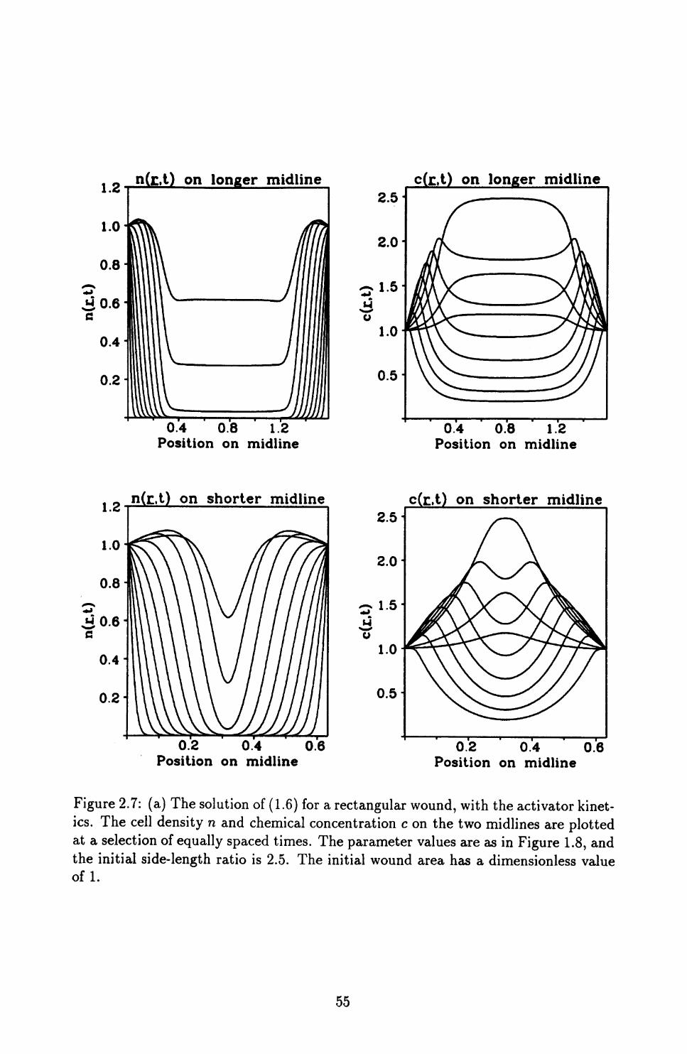
n(r.t) on longer midline c(£.t) on longer midline

0.4 0.8 1.2 Position on midline

0.4 0.8 1.2 Position on midline

n(E.t) on shorter midline c(r.t) on shorter midline

0.2 0.4 0.6 Position on midline

2.5

0.2 0.4 0.6 Position on midline

Figure 2.7: (a) The solution of (1.6) for a rectangular wound, with the activator kinet­ ics. The cell density n and chemical concentration c on the two midlines are plotted at a selection of equally spaced times. The parameter values are as in Figure 1.8, and the initial side-length ratio is 2.5. The initial wound area has a dimensionless value of 1.

55

n(r,t) on longer midline c(r,t) on longer midline

0.4

0.2

0.4 0.8 1.2 Position on midline

0.4 0.8 1.2 Position on midline

n(r.t) on shorter midline

0.6

0.4

0.2

0.2 0.4 0.6 Position on midline

c(r.t) on shorter midline

02 0.4 0.6 Position on midline

Figure 2.7: (b) The solution of (1.6) for a rectangular wound, with the inhibitor kinet­ ics. The cell density n and chemical concentration c on the two midlines are plotted at a selection of equally spaced times. The parameter values are as in Figure 1.8, and the initial side-length ratio is 2.5. The initial wound area has a dimensionless value of 1.

56

Activator

Inhibitor

Figure 2.8: The wound edge at a selection of equally spaced times for an initially rectangular wound. The 'wound edge' is defined as the contour n = 0.8. The param­ eter values are as in Figure 1.8, and the initial side-length ratio is 2.5. The initial wound area has a dimensionless value of 1.

57

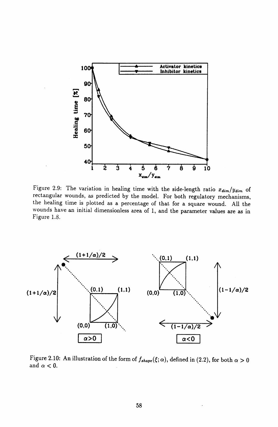
Activator kinetics Inhibitor kinetics

40-

Figure 2.9: The variation in healing time with the side-length ratio Xdim/Vdim of rectangular wounds, as predicted by the model. For both regulatory mechanisms, the healing time is plotted as a percentage of that for a square wound. All the wounds have an initial dimensionless area of 1, and the parameter values are as in Figure 1.8.

\

\«U) (1,1)

(0,0) (l,0)\

I a>0

\(0,l) (1,1)

(0,0) (1.0)\

a<0

Figure 2.10: An illustration of the form of fshape (^ a), defined in (2.2), for both a > 0 and a < 0.

58

Figure 2.11: The family of wound shapes defined by (2.2), parameterized by a. For clarity, all the shapes are illustrated with the same midline lengths, but in the numerical simulations, the lengths of the midlines are chosen, in a specified ratio, so that in each case the initial wound area has a dimensionless value of 1.

but in the numerical simulations, the lengths of the midlines are chosen, in a spec­

ified ratio, so that in each case the initial wound area has a dimensionless value of

1. Figure 2.12 illustrates the solutions of the model (1.6) for a — —0.8, with midline

lengths Xdim and ydim in the ratio 1.5, and the corresponding wound edge contours

are shown in Figure 2.13. The solutions and contours for a = +0.8 are shown in

Figures 2.14 and 2.15, respectively, again with Xdim/ydim = 1-5.

The variation in healing time with the parameter a, as predicted by the activator

and inhibitor mechanisms, is shown in Figure 2.16. It appears that this variation is

similar for the two mechanisms when the wound shape is concave when viewed from

the centre, but quite different for convex wound shapes. To investigate this further,

\ve considered a second family of wound shapes, given by

/.fcape(£;p)=£ P , 0<p<00. (2.3)

This family is illustrated in Figure 2.17; as the parameter p increases from zero, the

wound changes from a highly cusped shape, through a diamond at p = 1, to an ovate

shape, and finally to a rectangle as p —> oo. Again, for clarity all the shapes are shown

with the same midline lengths, but in the numerical simulations, these lengths are

chosen so that the initial wound area has a dimensionless value of 1 in each case. The

variation in healing time with the parameter p, as predicted by the two regulatory

59

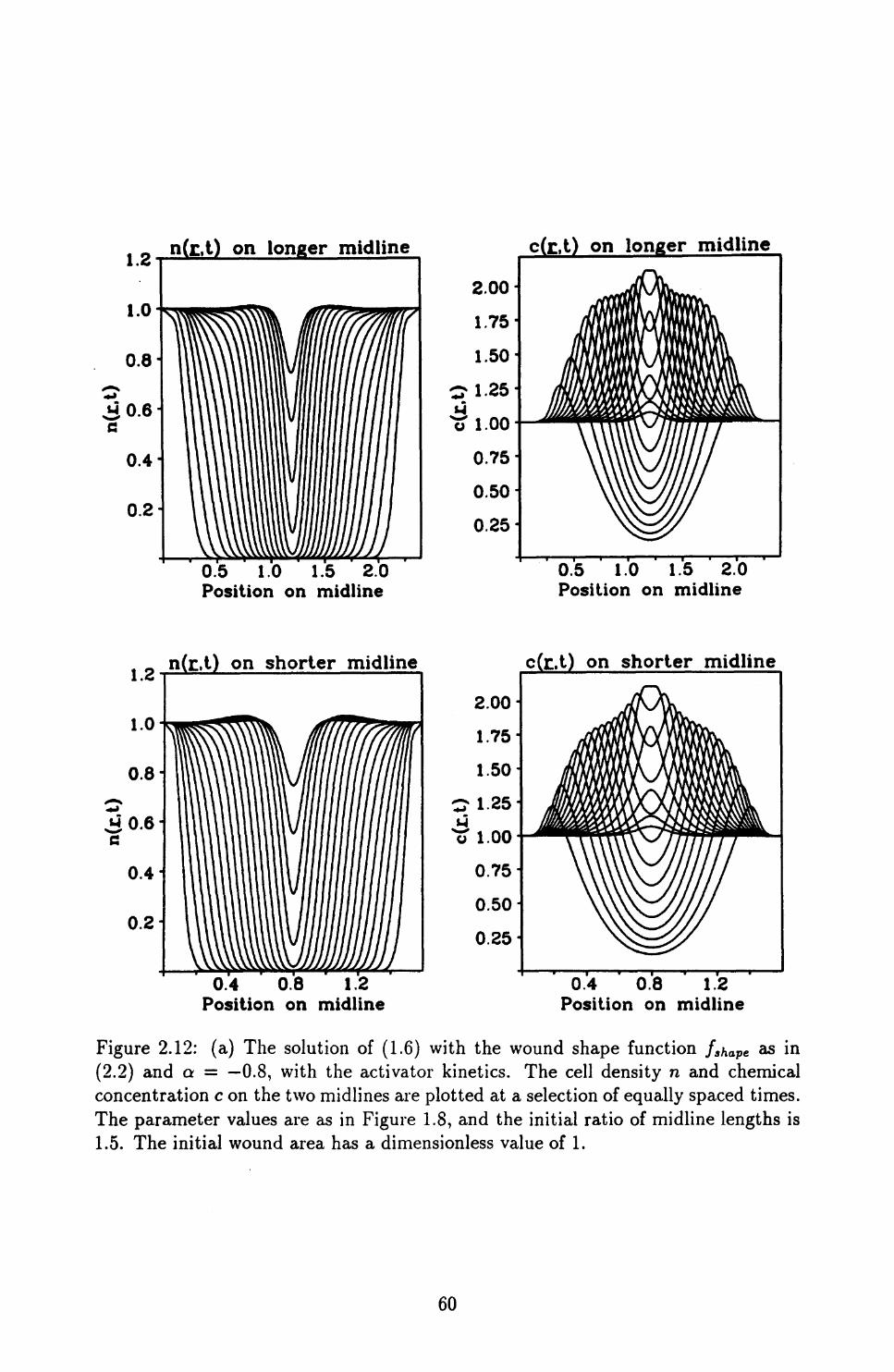
n(r.t) on longer midline c(r,t) on longer midline

0.5 1.0 1.5 2.0 Position on midline

0.5 1.0 1.5 2.0 Position on midline

n(r.t) on shorter midline c(c.t) on shorter midline

0.4 0.8 1.2 Position on midline

0.4 0.8 1.2 Position on midline

Figure 2.12: (a) The solution of (1.6) with the wound shape function fahape as in (2.2) and a = —0.8, with the activator kinetics. The cell density n and chemical concentration c on the two midlines are plotted at a selection of equally spaced times. The parameter values are as in Figure 1.8, and the initial ratio of midline lengths is 1.5. The initial wound area has a dimensionless value of 1.

60

n(r.t) on longer midline c(r,t) on longer midline

1 2 3 Position on midline

qo.e tf

0.4

0.2

1 2 3 Position on midline

n(r.t) on shorter midline c(r.t) on shorter midline

0.4 0.8 1.2 Position on midline

0.8-

0.4

0.2

0.4 0.8 1.2 Position on midline

Figure 2.12: (b) The solution of (1.6) with the wound shape function fskape as in (2.2) and a = —0.8, with the inhibitor kinetics. The cell density n and chemical concentration c on the two midlines are plotted at a selection of equally spaced times. The parameter values are as in Figure 1.8, and the initial ratio of midline lengths is 1.5. The initial wound area has a dimensionless value of 1.

61

Activator

Inhibitor

Figure 2,13: The wound edge at a selection of equally spaced times with the wound shape function f$hape as in (2.2) and a = —0.8. The 'wound edge' is defined as the contour n = 0.8. The parameter values are as in Figure 1.8, and the initial ratio of midline lengths is 1.5. The initial wound area has a dimensionless value of 1.

62

1.2 n(r.t) on longer midline c(r,t) on longer midline

0.4 0.8 1.2 Position on midline

0.4 0.8 1.2 Position on midline

n(r.t) on shorter midline c(r.t) on shorter midline

0.2 0.4 0.6 0.8 Position on midline

0.2 0.4 0.6 0.8 Position on midline

Figure 2.14: (a) The solution of (1.6) with the wound shape function fshape as in (2.2) and a = 0.8, with the activator kinetics. The cell density n and chemical concentration c on the two midlines are plotted at a selection of equally spaced times. The parameter values are as in Figure 1.8, and the initial ratio of midline lengths is 1.5. The initial wound area has a dimensionless value of 1.

63

n(r.t) on longer midline c(r,t) on longer midline

0.4 0.8 1.2 Position on midline

0.4

0.2

0.4 0.8 1.2 Position on midline

n(r.t) on shorter midline c(r.t) on shorter midline

0.4

0.2

0.2 0.4 0.6 0.8 Position on midline

0.2 0.4 0.6 0.8 Position on midline

Figure 2.14: (b) The solution of (1.6) with the wound shape function fahape as in (2.2) and a = 0.8, with the inhibitor kinetics. The cell density n and chemical concentration c on the two midlines are plotted at a selection of equally spaced times. The parameter values are as in Figure 1.8, and the initial ratio of midline lengths is 1.5. The initial wound area has a dimensionless value of 1.

64

Activator

Inhibitor

Figure 2.15: The wound edge at a selection of equally spaced times with the wound shape function fshape as in (2.2) and a = 0.8. The 'wound edge' is defined as the contour n = 0.8. The parameter values are as in Figure 1.8, and the initial ratio of midline lengths is 1.5. The initial wound area has a dimensionless value of 1.

65

102

Activator kinetics Inhibitor kinetics

-1.0

Figure 2.16: The variation in healing time with the parameter a as predicted by the model, with the wound shape function fshape(£', «) as defined in (2.2). For both regulatory mechanisms, the healing time is plotted as a percentage of that for a diamond-shaped wound, given by a = 0. All the wounds have an initial dimensionless area of 1 and midline length ratio of 1.5, and the parameter values are as in Figure 1.8.

p=oo

Figure 2.17: The family of wound shapes defined by (2.3), parameterized by p. For clarity, all the shapes are illustrated with the same midline lengths, but in the nu­ merical simulations, the lengths of the midlines are chosen, in a specified ratio, so that in each case the initial wound area has a dimensionless value of 1.

66

100-

90-

I 801

9•< 7010)

OS60

50 Activator kinetics Inhibitor kinetics

0.0 0.5 1.0 1.5p (if p<l) or 2-1/p (if p>l)

2.0

Figure 2.18: The variation in healing time with the parameter p as predicted by the model, with the wound shape function fshape(£', P) as defined in (2.3). For both regulatory mechanisms, time is plotted as a percentage of that for a diamond-shaped wound, given by p = 1. To give equal emphasis to convex and concave wound shapes, we plot the relative healing time against p when p < 1, and against 2 — l/p when p > 1. All the wounds have an initial dimensionless area of 1 and midline length ratio xdim/ydim = 1.5, and the parameter values are as in Figure 1.8.

mechanisms, is shown in Figure 2.18. These results again suggest that the variation

in healing time is similar for the two mechanisms when the wound shape is concave

when viewed from the centre, but quite different for convex wound shapes.

An explanation for this trend is suggested by the wound edge contours in Fig­

ures 2.13 and 2.15. The first of these figures shows that for a highly cusped (that

is, concave when viewed from the centre) wound shape, the wound edge rounds up

during healing, for both the activator and inhibitor kinetics, and is almost circular as

the wound closes. In contrast, for the convex wound shape illustrated in Figure 2.15,

the wound edge tends to flatten out, so that the ratio of midline lengths increases

during healing. Moreover, this increase is significantly greater for the inhibitor kinet­

ics than for the activator kinetics. Now for a given initial wound area, the healing

time will be shorter if the wound edge tends to flatten out more during healing,

since the wound perimeter is then greater; this trend was discussed for rectangular

wounds on page 54. Thus the differences between concave and convex wound shapes

67

in Figures 2.16 and 2.18 can be explained in terms of shape change during healing.

This explanation raises an important question: what are the key factors control­

ling the extent to which an ovate wound flattens out during healing that is governed

by the model equations? We were able to answer this by returning to the basic

model (1.1), in which chemical regulation of mitosis is neglected. We rescale the

dimensionless time coordinate in (1.1) so that the model equation is

(2.4)

In this form, the model has a single dimensionless parameter F, which reflects the

relative contributions of mitosis and diffusion to the healing process. The wound edge

contours predicted by this basic model are shown in Figure 2.19 for a range of values

of F, for a wound that is initially elliptical with midline length ratio 2. The wound

edge becomes more flattened during healing as F increases, and this is quantified in

Figure 2.20, in which we plot against F the midline length ratio of the wound when

its area has decreased to 10% of its initial value. This figure shows that shape change

during the healing of an ovate wound is a competitive process, with diffusion tending

to cause rouncling up of the wound, while mitosis tends to cause the wound to flatten.

In contrast, both diffusion and mitosis tend to cause a concave wound to round up

during healing.

Returning to the full model (1.6) with biochemical regulation of mitosis, it is now

clear why ovate wounds flatten more during healing with the inhibitor kinetics than

with the activator kinetics. The extent to which post-wounding mitosis is stimulated

by biochemical effects is approximately the same for the two mechanisms; however,

the determination of diffusion coefficients by fitting to experimental data, which we

discussed in Section 1.4, gave the cellular diffusion coefficient D to be 5 times larger

for the activator kinetics than for the inhibitor kinetics.

68

r-o.s r=i.o r-2.0

r^io.o

Figure 2.19: The wound edge at a selection of equally spaced times for a wound that is initially elliptical with midline length ratio 2 and dimensionless area 1, as predicted by the basic model (2.4), for a range of values of F. The wound becomes more flattened during healing as F increases.

69

Figure 2.20: The midline length ratio of a wound near to closure, when its area reaches 10% of its initial value, as predicted by the basic model (2.4), plotted against P. In each case, the wound is initially elliptical, with midline length ratio 2 and dimensionless area 1.

2.4 ConclusionsIn this chapter and Chapter 1, we have developed a reaction-diffusion model for epi­

dermal wound healing in which the parameter values are based as far as possible on

experimental results. Numerical solutions of the model with either chemical acti­

vation or inhibition of mitosis compare well with experimental data on the normal

healing of circular wounds, supporting the view that biochemical regulation of mitosis

is fundamental to the process of epidermal migration in wound healing. Analytical

investigation of the solutions as travelling waves was possible in one spatial dimen­

sion. We studied the travelling wave system of ordinary differential equations under

two biologically relevant approximations, which clarified the accuracy of these ap­

proximations and the roles of the various model parameters in the wave form and the

speed of healing. We went on to perform 'mathematical experiments', from which we

made experimentally testable predictions on the effects of adding mitotic regulators

to healing wounds, and on the variation of healing time with wound shape. This

latter investigation led to an understanding of the competitive processes controlling

changes in wound shape during healing. It may be possible to exploit the differ­

ences in such shape changes as predicted by the activator and inhibitor kinetics to

distinguish experimentally between these two regulatory mechanisms.

70

Chapter 3

The Response of Embryonic Epidermis to Wounding:

a Basic Model

3.1 Biological BackgroundThe process of cells crawling across exposed connective tissue to close adult epidermal

wounds has been described in detail in the Introduction and Section 1.1. Although de­

bate continues on many aspects of adult epidermal wound healing, this basic process

of lamellipodial migration is well established. In contrast, the mechanisms underlying

the healing of embryonic epidermal wounds remain largely unknown. Recently, the

process has been studied in detail by Martin and Lewis (1991a,b). Using a tungsten

needle, they made lesions on the dorsal surface of four-day chick embryonic wing buds.

These wounds were 0.5mm square, with thickness O.lmm, so that the basal lamina

was cut and there was some bleeding. They healed perfectly and rapidly, typically

in about 24 hours. Although the epidermis moved actively across the contracting

mesenchyme, they found no evidence of lamellipodia at the wound front in either

the basal or peridermal layers (Figure 3.1). This absence of lamellipodia was consis­

tent with a second observation: when a small island of embryonic skin was grafted

onto a denuded region of the limb bud surface, the grafted epidermis, far from ex­

panding over the adjacent exposed mesenchyme, actually contracted, leaving its own

mesenchyme exposed. This phenomenon suggested that the mechanism underlying

epidermal movement might be a circumferential tension at the free edge, acting like a

purse string. Such a mechanism would cause contraction of both an epidermal island

and a hole in the epidermis.

Martin and Lewis (1991a,b) pursued this possibility further by staining spec-

71

imens with fluorescently tagged phalloidin, which binds selectively to filamentous

actin (Faulstich et a/., 1983; Wulf et a/., 1979), and thus reveals the distribution of

filamentous actin in the healing wounds. Actin is the most abundant protein in many

eukaryotic cells, often constituting more than 5% of the total cell protein. It exists

in two forms, unpolymerized ('globular actin') and polymerized ('filamentous actin'),

and typically about half of the actin molecules in a cell are polymerized. Actin

filaments, also known as microfilaments, are held in three-dimensional networks by

cross-linking proteins; the resulting microfilament network is a fundamental part of

the cell cytoskeleton, and is responsible for many aspects of cellular mechanics. Al­

berts et al. (1989, Chapters 11 and 14) present a detailed review of the role of actin in

the cytoskeleton. Filamentous actin is therefore an obvious candidate for the protein

causing this purse string effect. Staining with phalloidin revealed a thick cable of

actin around almost all of the epidermal wound margin (Figure 3.2), localized within

the leading layer of basal cells. The cable appeared to be continuous from cell to cell,

presumably via adherens junctions, except at a very few points. The thickness of the

cable did not change noticeably during healing: it was present certainly within an

hour of wounding, and persisted until the wound was closed.

To gauge more accurately the time course of the establishment of the actin cable,

Midwinter et al. (in preparation) have investigated simple slash wounds running

along the proximodistal axis of the limb. This lesion takes only seconds to make, as

opposed to the 5-10 minutes required to dissect a square of skin from the limb bud.

The slash lesion data indicate that the actin cable begins to form within minutes of

wounding. In this chapter and Chapter 4 we investigate, from a theoretical point of

view, the formation of the actin cable as a response to wounding. Specifically, we use

a mathematical model to address the possibility that the cable forms by compaction

and reorientation of the actin filament network, without either depolymerization of

actin in one part of the cell and corresponding repolymerization in another part, or

de novo synthesis of filamentous actin. The results of our modelling enable us to

suggest a possible mechanism for the formation of the actin cable.

72

Figure 3.1: bcanning electron micrograph ot a wound edge in chick embryonic epi­ dermis, 12 hours after the operation. The wound was made by removing a square patch of embryonic skin from the dorsal surface of the wing bud at 4 days of in­ cubation (stage 22/23). The epidermis overlies the flattened surface of the exposed mesenchyme. Note the smooth edge of the epidermis and the absence of lamellipodia.

Figure 3.2: The epidermal wound front on the dorsum of a, chick wing bud after 12 hours of healing, as seen in optical section by confocal scanning laser microscopy. The tissue has been stained with rhodamine-labelled phalloidin, which binds to filamen­ tous actin, and the sections are parallel to the plane of the epidermis. The epidermis is at the lower left, with the exposed mesenchyme (largely below the plane of section) at the upper right, (a) Superficial section, in the plane of the periderm, whose broad flat cells are outlined by their cortical actin. (b) Section about 4/tm deeper, in the plane of the basal epidermal cells, showing the actin cable at the wound front.

73

3.2 The Mechanical Approach to ModellingAt the developmental stages at which the experiments discussed above (Martin and

Lewis, 1991a,b) were performed, the embryonic epidermis is two cell layers thick,

consisting of a superficial, pavement-like periderm layer and a cuboidal basal layer.

The actin cable develops in the basal layer, and it is to this layer that our modelling

considerations apply. The basal cells form a confluent sheet of cells, attached to

the underlying basal lamina at focal contacts (see, for example, Alberts et a/., 1989,

Chapter 11). We model the initial response of this sheet to wounding by modifying the

mechanochemical model for the deformation of epithelial sheets proposed by Murray

and Oster (1984). This was the first continuum mechanochemical model for epithelial

morphogenesis, and was based on the discrete model of Odell et al. (1981). Murray

(1989) gives an in depth review of mechanical models for morphogenesis.

The model of Murray and Oster (1984) treats the epithelial sheet as a linear,

isotropic, viscoelastic continuum, an approach which the authors justify as a rea­

sonable first approximation in the absence of detailed knowledge of the mechanical

properties of cytogel, and which is discussed from a rheological viewpoint by Elson

(1988). In Murray and Oster's (1984) model and other related models (see Murray,

1989), cellular contraction forces are controlled by the concentration of free calcium.

We modify this model to investigate the new equilibrium reached by the basal cell

sheet after wounding. Since we are only interested in the equilibrium state, chemical

control is equivalent to an imposed spatial variation in parameter values; we neglect

such affects, and assume that the mechanical properties of the cell sheet change only

in response to the local stress and strain fields. Following wounding, the cytoskele-

ton undergoes rapid changes, on a time scale of a few minutes (Midwinter et a/., in

preparation), reaching a new state which is the "quasi-equilibrium" we are consider­

ing. Of course, this new state also changes over a time scale of a few hours, as healing

proceeds, but we do not consider the processes occurring on this longer time scale.

The mechanical properties of a confluent cell sheet are determined largely by the

intracellular actin filaments (Pollard, 1990). In epithelial sheets, cell-cell adherens

junctions form a continuous 'adhesion belt' around the cell, just below the tight

74

Figure 3.3: Adhesion belts between epidermal cells. This belt-like intercellular junc­ tion encircles each of the interacting cells, linking the intracellular actin filaments in a transcellular network.

junctions, as illustrated in Figure 3.3. These adherens junctions are connection sites

for actin filaments, and thus the intracellular actin filaments are linked, via transmem-

brane proteins at the adhesion belt, in a transcellular network. Our model addresses

the equilibrium state of this network.

At equilibrium, the stress tensor in the cell sheet is taken to be

elastic stress

rGL

activecontraction

stress

(3-1)

where u(r) is the displacement of the material point initially at r, the strain tensor £ = |(Vu + Vwr), G(r} is the density of intracellular actin filaments at the material point initially at r, E and F are positive constants, and / is the unit tensor. As discussed below, the traction stress per filament, r, is in general a function of the local compaction. The exertion of traction forces by fibroblasts has been extensively studied (see, for example, Harris, 1982; Stopak and Harris, 1982), and traction forces have been observed in a range of other cell types, including chick embryonic corneal

epithelial cells (Mattey and Garrod, 1984). The elasticity of the actin filament net-

75

work arises from the extensive interpenetration of the long actin filaments, which

tends to immobilize them (Janmey et a/., 1988). The form (3.1) is used extensively

in the literature: see, for example, Oster et al. (1983), Murray and Oster (1984),

Oster (1984), Oster et al (1985), Murray et al (1988). In contrast to the majority

of these models, (3.1) has no viscous contribution because we are considering the

equilibrium situation.

At equilibrium, these elastic and traction forces balance the elastic restoring forces

that arise from attachment to the substratum. The importance of such attachments

is illustrated in recent experiments by Hergott et al (1989) on the response of chick

embryonic corneal cells to wounding in an organ culture system. In this study, cells

migrate into the wound along the exposed basal lamina. They find that focal contacts

form with the basal lamina at the ends of actin filament bundles, and they attribute

the considerable tensile forces generated by the migrating cells to the interaction

of actin filament bundles with the substratum, via these focal contacts. Following

Murray and Oster (1984), we model these restoring forces by \Gu, where the positive

constant A reflects the strength of the attachments. The term is proportional to G

since most of the intracellular actin filaments terminate at, or close to, a region of

adhesion to the substratum (Alberts et a/., 1989, Chapter 11). Hergott et al (1989)

also present direct experimental evidence for this proportionality: they find that the

density of focal contacts increases in parallel to that of actin filament bundles in the

response to wounding. A similar observation was made by Wechezak et al (1989) in

experiments on the cytoskeletal response of isolated endothelial cells to shear stress,

applied using a flow chamber.

Thus the equation to be solved for the new equilibrium configuration is

V • £ - \Gu = 0 (3.2)

with a_ as in (3.1). We treat the cell sheet as infinite, which is a valid approximation

provided the wound area is small compared to the whole sheet, which certainly holds

in the experiments of Martin and Lewis (1991a,b) discussed in the previous section.

Thus the boundary conditions are w(oo) = Q, and q_ • n = Q, at the free edge, where

76

n is the unit vector normal to this edge. Our approach in deriving (3.1), (3.2) and

the boundary conditions assumes that in the pre-wounding state, u = Q everywhere.

This is not an entirely trivial assumption in a developing embryo, but observations

of the epithelial sheet prior to wounding indicate that, to a good approximation,

the cell density is uniform and the substratum attachments are reforming sufficiently

fast that the restoring forces exerted by them are negligible (Paul Martin, personal communication, 1990).

A crucial feature of the model (3.2) is the relationship between G and u. In this

chapter we address the question of whether the actin cable observed by Martin and

Lewis at the wound edge could be formed simply as a result of compaction- and stress-

induced changes in filamentous actin density. Specifically, we make the following key assumption:

the response to wounding involves neither depolymerization of actin in

one part of the cell and corresponding repolymerization in another part,

nor de novo synthesis of filamentous actin, nor intracellular movement of

intact actin filaments, so that the amount of filamentous actin in a given

region of cytogel remains constant as that region is deformed.

The time scale over which the actin cable forms (a few minutes) is certainly consistent

with this assumption, but does not exclude actin polymerization. For instance, on

sudden exposure to a chemoat tract ant peptide, neutrophils form pseudopodia over

their entire surface, and the proportion of intracellular actin that is polymerized rises

from about 30% to about 60% in 20 seconds (Carson et a/., 1986).

There is limited experimental evidence that this is the mechanism of cytoskeletal

reorganization in some other systems. In a study on chick heart fibroblasts, Chen

(1981) found that following removal from the substratum, the mesh of actin filament

bundles in the fibroblast tails rearranged from a nonuniform to a uniform, random

arrangement by reorientation, without any disassembly or reassembly of actin fila­

ments. In more recent experiments involving micromanipulation of cellular protru­

sions in 3T3 cells, Albrecht-Buehler (1987) found that the expression of tension in

77

the cells was insensitive to the chemical cytochalasin B, which inhibits the polymer­

ization of actin monomers (see page 146). Thus, while Albrecht-Buehler's findings do

not preclude microfilament depolymerization, they can be explained more naturally

by a simple reorientation of the filaments. Albrecht-Buehler also found that when

detached from the substratum, cellular protrusions shortened by 20-50% within a few

seconds, with further relaxation to equilibrium over 3-5 minutes. These time scales

of cytoskeletal reorganization are consistent with those for the formation of the actin

cable found by Midwinter et al. (in preparation). Thus, we assume that the amount

of filamentous actin in a given region of cytogel remains constant as that region is

deformed, so that G(\ — A) = AC, a spatially independent constant. Here A is the

fraction of its pre-wounding volume by which a small region of cytogel contracts in

the response to wounding. Substituting this into (3.2) gives the governing equation

as

~-=Q - (3 - 3)In this chapter we approximate A as the negative dilation, that is A « — V • u,

following classical linear elasticity theory (see, for example, Segel, 1977a). However,

this approximation is reconsidered in Section 4.1.

It remains to consider the functional form of r, the traction stress per filament.

When a region of the actin filament network is compressed, the degree of filament

overlap increases. Consequently additional myosin cross-bridges form between actin

filaments (Oster and Odell, 19S4a), with a corresponding increase in the traction

stress per filament. (The role of myosin in the contractile forces exerted by actin fil­

aments is discussed in detail in the book by Alberts et a/., 1989, Chapter 11; see also

page 137). This is effectively a synergy phenomenon: actin filaments together exert

a greater traction force than the sum of the traction forces they exert separately. We

model this synergy effect by taking T to be an increasing function of the local com­

paction A, following previous mechanochemical models of epithelium (Oster, 1984;

Oster and Odell, 1984a,b; Oster et a/., 1985). Specifically, we take T = r0 /(l — /?A).

With this form for r, a decrease in dilation at a point causes an increase in the cell

traction stress at that point both because of an increase in the actin filament density

78

at the point and because of an increase in the traction stress per filament. Intu­ itively, we expect the former effect to be larger than the latter, and we thus require that ft < 1. With this constraint, r is bounded, since A < 1 (a region cannot be compressed to a point). When discussing model solutions, we will consider not only 0 < j3 < 1, but also the case 0 = 0. This corresponds to the traction stress per actin filament being independent of dilation, so that the effects of additional myosin cross-bridging are neglected. This is the form used by Murray and Oster (1984) in the first continuum mechanochemical model for epithelial morphogenesis.

To clarify the roles of the various model parameters, we nondimensionalize (3.3) by defining

r* = r/L IL = IL/L E* = E/r0 r = T/TQ A* = \a2/r0

where * denotes a dimensionless quantity and L is a typical linear dimension of the wound; for circular wounds we take L to be the initial wound radius. Substituting these into (3.3) with A = — V-w, and dropping the asterisks for notational simplicity, gives

V- AM = Q. (3.4)1 + V-u

As in other applications of mechanochemical models, the experimental data cur­ rently available to give estimates for parameter values is very limited, and is in fact insufficient to determine any of the dimensionless parameters in equation (3.4). For completeness, however, we briefly review the few relevant quantitative experiments. There are a number of studies which address the mechanical properties of actin gels from a rheological viewpoint, for instance Jen et al. (1982), Sato et al. (1985), Sato et al. (1987), Zaner and Hartwig (1988), Janmey et al. (1988). The rheological ter­ minology they use is explained in the book by Ferry (1980). Typically, these studies consider an actin gel held between two plates, with the lower plate oscillating sinu- soidally. The phase difference and amplitude ratio of the displacements of the upper and lower plates are recorded, enabling the storage elastic modulus and loss (viscous) modulus to be calculated as a function of frequency (see Ferry, 1980, for details). The

79

study by Janmey et al (1988) calculates similar quantities using a torsion pendulum

apparatus. Unfortunately, these quantities are not sufficient to calculate any of the

parameters in our representation of the viscoelastic continuum, which is a simplifi­

cation of that used in rheological treatments. There is also a relevant quantitative

study by Dennerll et al. (1988) on tension and compression in neurites. They record

rest tensions and spring constants by applying a force with a calibrated glass needle.

These values could be used to calculate (E + F) and TO, but this would not be suffi­

cient to determine any of the parameters in our dimensionless model equation (3.4).

Also, these experiments are on a very different cell type, and the results vary over

several orders of magnitude.

We treat the basal cell layer as two-dimensional, which is a reasonable assump­

tion since its thickness is about lO^m, compared to the wound dimensions of about

500//m in the experiments of Martin and Lewis (1991a,b). In fact the adhesion belt

confers a genuinely two-dimensional structure on the transcellular actin filament net­

work (Figure 3.3). We consider the full radially symmetric two-dimensional problem

in Section 3.4. First we investigate the solutions of the dimensionless governing equa­

tion (3.4) in one spatial dimension.

3.3 One-Dimensional SolutionsSolutions of the model in one spatial dimension are important for two reasons. Firstly,

a study of the one-dimensional equations increases our mathematical understanding

of the system, which can then be extended to the more biologically relevant two-

dimensional equations. Secondly, the solutions may be applicable to regions of square

wounds away from the corners, so that the one-dimensional model solutions can be

compared to some aspects of the data from the experiments of Martin and Lewis

(1991a,b) discussed in Section 3.1.

In one spatial dimension, the dimensionless governing equation (3.4) is

y-dx -f ux + pu 1 + u

80

with boundary conditions

(E + F)t/x + ——-— = 0 at x = 0 and u = 0 at x = oo, (3.6) 1 + ftux

where ux denotes du/dx, and we take x = 0 to be the wound edge. Integrating this equation and using the boundary condition at x = oo gives

(3.7)z

where if ft ^ 1

P(ux ] = (E + F) [tir - log(l + ux }\ + -^-^ log(l + I/.)

1 + i, (3.8a)

and if ^ = 1

ur ) = (E + I>x - (JE + T + 2) log(l + ux ) - —— + 2 . (3.8b)1 + ux

The case ft = I is not relevant biologically, but we will consider it briefly for mathe­ matical completeness. We write the boundary condition at x — 0 in (3.6) as

Q(ux ) = (E + r)ftul + (E + T)Ux + 1 = 0. (3.9)

3.3.1 Existence and uniqueness of solutionsWe now prove that (3.7) subject to (3.9) has a unique monotonically decreasing solution satisfying ux > — 1 if and only if

E > r-—Q and 0 < ft <

or E> 4/? and ft> 1/2

The condition ux > — 1 is a physical constraint: a region cannot be compressed to a point. Here, and throughout the derivation of these conditions, we write E — (E + T) for notational simplicity.

Consider first the case ft < 1. As discussed above, this is the case of interest biologically; we consider ft > 1 later for mathematical completeness. The form of

81

P(ux ) on -1 < ux < 0 depends on E and (3. For E > 1/(1 - /?), P(tO -> +00 as

MX -> -1, while for E < 1/(1 - /?), P(ux ) -> -oo as ux -» -1. For E = 1/(1 - /?),

_ ( l) ~ _ _ g(0(1-0) -ft(l-ft)2-ft

This is strictly positive when 0 < ft < 1, since then [(2 — 0)/(0(l — /?))] > 0, and also

- log(l -d_

d0

with

so that

Differentiating (3.8a) with respect to ux gives

(2 - 0)*(1 - (3) >0

2-0-w

- log(l - = 0 when 0 = 0,

> 0 when 0 < 0 < 1

Eu, u.

2-

P'(ux ) =

P"(ux ) =

Thus P'(0) = 0 and, after simplification, P"(0) = E - (1 + 0). Thus for small u

P(ux ) has the same sign as E — (1 + 0).

Apart from the root at ux = 0,

XI

P'(ux ) = 0 (3ux ) 2 = (3(1 + ux )

+ 20(E - IK +

<^ u = (^~E)±\/E0-E + 1E{3

These roots are real if and only li E < 1/(1 — 0). Then the larger (less negative) root

lies in [—1,0) if E > 1+0, and is positive if E < 1 + /?; the smaller (more negative)

root is less than —1. For

E/3<0 \/E0 -E + KE-1

E > 1 and E0 - E + 1< (E - I) 2

£>!+/?;

82

Eftwhich is trivially satisfied

provided E ^ !/(!-/?), in which

case the root is equal to — 1 ;

EftEft-E + Kl,

since E < 1/(1 -

ft<l.

A

Taking all these considerations into account, the form of P(ux ) as E and ft vary is as

shown in Figure 3.4.

The roots q± of the boundary condition Q(ux ) = 0 are

-E ± \/E2 - 4 q — ———— v__ ______ _2Eft

These are real if and only if E > 4/3, in which case they are both negative. Now

0(0) = 1 and Q(-l) = E(ft - 1) + 1. Thus if E > 1/(1 - ft), exactly one root of the

quadratic Q lies in (-1,0), that is

</+ € (-1,0) and q. < -1 if E > — — r . (3.10)

Conversely, if 4(3 < E < 1/(1 - ft), both roots of Q lie in (-1,0) if qmin € (-1,0),

and both roots are less than —1 if qm {n < — 1. Here qmin is the value of ux minimizingA

(5, and straightforward differentiation gives qmin — —1/2/3. Thus when 4(3 < E <

-1< q+1 q- < 0 if ft > 1/2 (3.11a)

q+,q.<-l if ft < 1/2. (3.11b)

We are now in a position to prove the conditions for the existence and uniqueness

of solutions of (3.7) subject to (3.9) in the case ft < 1. From the forms of P(ux )

83

(-1.0)

(-1.0)

X•o

•o

X•o3•o

du/dx (0,0)

(-1.0)

(0.0)

(0,0)

du/dx0,0)

3 •O

X•o3 •o

A_

Figure 3.4: The qualitative form of the function P(wr ), given in (3.8), as £ and /? vary with ft < 1. (a) E > 1/(1 - /?); (b) j& = 1/(1 - /?); (c) (1 + /?) < E < 1/(1 - /?);

84

in Figure 3.4 and results (3.10) and (3.11), it is clear that if E > 1/(1 - /?) there

is a unique monotonically decreasing solution of (3.7) subject to (3.9). For then

P(ux ) decreases monotonically from +00 to zero on (—1,0]. Thus given any u > 0,

there is exactly one value of ux 6 (-1,0] satisfying the governing equation (3.7),

and moreover exactly one of the roots for ux of the boundary condition (3.9) lies in

(-1,0).

In addition, if 1 + ft < E < 1/(1 — /?), there is a unique monotonically decreasing

solution provided {3 > 1/2, E > 4/? (so that q± are real) and q. < pmax < <7+; we

prove below that the first two of these conditions together imply the third. Here pmax

is the value of ux at which P attains its maximum on ( — 1,0), that is

_Pmax -

For then P(ux ) decreases monotonically to zero on [pmar ,0]. Thus there is a 1-1

correspondence between u € [0, P(pmax)\ and ux £ [pmair,0], given by the governing

equation (3.7). Moreover, exactly one of the roots for ux of the boundary condition

(3.9) lies in (Pmax,®)- Note that 0 > 1/2 and E > 4/5 together imply that theA,

condition E > 1 + (3 is satisfied. Moreover, these three conditions are necessary

when 1 + P < E < 1/(1 - /?) except for the case of E = 4/5. But then if 0 > 1/2,

Pmax = q+ = q~ = — 1/2/5, and thus there is a unique monotonically decreasing

solution, while if 0 < 1/2, q+ = q_ = — 1/2/5 < pma.x, and thus there is no solution.

For completeness, we now consider solving (3.7) as an initial value problem in theA

parameter domain 4/5 < E < 1/(1 — /?), /5 > 1/2, with 1^(0) = <?_. Although

this does not give a solution of (3.5) subject to (3.6), the boundary condition (3.9) at

x = 0 is satisfied. The solution follows the curve P(ux ), the form of which is shown

in Figure 3.4c, in the direction of decreasing ux . Thus u decreases monotonically, and

u = 0 at some finite value of x, with the corresponding slope ux being the unique root

of P on (—1,0). As x continues to increase, u becomes negative so that u2 increases

again, and the solution follows the curve P(ux ) back in the direction of increasing

wx , passing through the point corresponding to the initial condition, but with u now

negative. Finally, at some finite value of x, ux = pmax and u = -2^fP(ux)/\. At

85

this point d(u2 )/dx is positive, but the curve P(ux ) has a local maximum, and thus

equation (3.7) cannot be integrated further. Intuitively one would expect the solution

to break down at this point, since a function does not have a local inverse on any

neighbourhood of a local maximum, and thus equation (3.7) cannot be inverted to

express ux as a function of u on any neighbourhood of ux — pmax-

We now prove that q. < pmax < q+ when 4(3 < E < 1/(1 - 0) and /? > 1/2. We

have that

q.<pmax «=> -y/& - 4E(3 <2-E + 2\/E/? - E

E2 - 4E3 > 2 - E + 2E0 - E

or 2 - E + 2y/E0 -E + l > 0

2(E/3 - E + 1) < (E - 2)\/£/? - E 4- 1

or 2yE0 -E+l >(E-2)

and pmax < q+ <=> 2 - E + 2E3 - E

<> -

or_____ _

2 - £ + 2/60 -E + l < 0

or 2^E^ -E+l < (E - 2)

-E+l < (E - 2)

In these inequalities, we use the fact that E > 4/2 and /? > 1/2 together imply that

E>2.A

Finally, for /? < 1, consider the outstanding case of E = !/(!—/?). Then P(ux ) has

the form shown in Figure 3.4b: P( — l) is finite and strictly positive, and P'(— 1) = 0.

But when E = 1/(1 — /?), the roots of Q are

86

du/dx

(-1/0,0)

a

[0,0)

^

(0,0)

>K

Figure 3.5: The qualitative form of the function P(ux ), given in (3.8a), as E and vary with 0 > 1. (a) E > 1 -f /3; (b) E < 1 + /3.

= -1 and q, = 1 - - < -1 if ft < 1/2

$_ = -! and ?+ = 1 - i € (-1,0) if ft > 1/2.

A

Thus when £ = 1/(1 — /?), there is a unique monotonically decreasing solution sat­

isfying ux > — 1 if and only if /? > 1/2.

For completeness, we now consider the case of /? > 1. If /? = 1, similar calculationsA

to those above show that P(ux ) has the qualitative form shown in Figure 3.4c if E > 2A

and that shown in Figure 3.4d if E < 2. Also, the roots of Q are real if and only

if E > 4, in which case — 1 < qmin < pmax < qmax < 0. Thus there is a unique

monotonically decreasing solution of (3.7) subject to (3.9) if and only if E > 4.

If (3 > 1, the form of P(ux ) is different. For then P(ux ) — >• — oo as ux — »• — (l//?)+ .

The qualitative form of P(ux ) on (-!//?, 0) depends on the sign of P"(0) = £-!-/?,

and the two cases are shown in Figure 3.5. Now Q(—l/(3) = 1 = <2(0). Thus,

provided E > 4/9 so that (J has real roots, both the roots, q+ and <?_, lie in ( — 1//3,0).

Moreover, the inequalities <?_ < pmax < q+ are still valid when E > 4/5. Thus when

/? > 1, there is a unique monotonically decreasing solution of (3.7) subject to (3.9) if

and only if E > 4/?. (When ^ = 4/9, 9. = 9+ = pmo* = -l/2j9, as for 1/2 < ft < 1).

87

3.3.2 Numerical solutionsWe solved (3.7) subject to (3.9) numerically as an initial value problem, with ux (Q) = q+, and with ux determined at each value of u as the unique value satisfying (3.7) on

-1 < ux <0if /3 < 1/2, and on pmax < ux < 0 if ft > 1/2. We solved this algebraic equation for ux as a function of u numerically, and we integrated the initial value

problem using a Runge-Kutta-Merson method. In order that the parameter values correspond to those in the two-dimensional solutions discussed in Section 3.4, we take L, the length scale in the nondimensionalization, to be 500//m, which is about 50 cell diameters.

In comparing the one-dimensional model solutions with data from the experi­ ments of Martin and Lewis (1991a,b) involving square wounds on embryonic chick wing buds, we look in particular for the model to capture the intense aggregation of

filamentous actin at the wound edge that constitutes the actin cable. However, we also require that the solutions capture the more superficial aspects of the response to wounding, that is the extent to which the various cell layers retract. It is difficult to gauge this accurately in the square lesions, both because of the time taken to make the wound (5-10 minutes) and because it is difficult to distinguish between epider­ mal and mesenchymal retraction, since the wound edges are so shallow. Neither of these problems arise in the simple slash wounds considered by Midwinter et al. (in

preparation), and their data indicate an epidermal retraction of about 60//m at the wound edge, with only the leading 4-5 cell layers significantly contracted. We found

that the model solutions were able to capture this second important aspect of the

data for a wide range of parameter values. We illustrate this in Figures 3.6 and 3.7,A

which also show the effect of variations in A, E and (3 on the form of the solution. However, to capture the phenomenon of the actin cable, that is G(x) having a sharp

A

peak at x = 0, required both ft < 1/2 and [E — 1/(1 - /?)] small and positive; recallA ___

that for (3 < 1/2, a solution exists if and only if E > 1/(1 - /?). There was therefore a

range of parameter values in which we were able to capture both aspects of the exper­

imentally observed response of the embryonic epidermis to wounding, as illustrated

in Figure 3.8.

88

0.14-

0.12-

0.10-

0.08-

0.06-

0.04-

0.02-

Effect of variations in A Effect of variations in E

5% incr. in X Ref. paraxns

6% deer, in X0.64 o.6s

6.14-

0.12-

o.io-3 0.08

0.06-

0.04-

0.02 6% incr. in fiRef. paraxns

5% deer, in t0.64 0.08

0.14-

0.12-

0.10-

0.08-

0.06-

0.64-

0.02-

Effect of variations in ft

5% incr. in 0Ref. params

6X deer, in P

0.64 0.08

Figure 3.6: The effect of parameter variation on the numerical solution for u(x) of (3.7) subject to (3.9). The solutions in green are for the parameter values A = 15.0, E = 1.25, ft = 0.15. Those in red correspond to a 5% increase in one parameter, and those in blue correspond to a 5% decrease in that parameter. The x-interval shown corresponds to the leading 5 cell layers. The solution is particularly sensitive to the decrease in E because the lower limit of 1/(1 — /?) is approached.

89

Effect of variations in X Effect of variations in E14-

12-

10-

s ^o'(

4-

2"

5X incr. in XBel. params

5X deer, in X

0.04 0.68

incr. in E Ref. params

6% deer, in

0.04 0.08

Effect of variations in jg5% incr. in Bet. params

5% deer, in

Figure 3.7: The effect of parameter variation on the filamentous actin density G(x) = 1/(1 4- Ua;), as predicted by the numerical solution of (3.7) subject to (3.9). The solutions in green are for the parameter values A = 15.0, E = 1.25, 0 = 0.15. Those in red correspond to a 5% increase in one parameter, and those in blue correspond to a 5% decrease in that parameter. The x-interval shown corresponds to the leading 5 cell layers. The solution is particularly sensitive to the decrease in E because the lower limit of 1/(1 - 0) is approached.

90

0.12

0.10

0.08

£•0.063

0.04-

0.02

a

0.04 0.08 0.04 0.08

Figure 3.8: (a) The numerical solutions of (3.7) subject to (3.9) for A = 3.0, E = 1.3, ft — 0.2303. (b) The corresponding dimensionless actin filament density G(x) = 1/(1 + ux ). This solution captures the key aspects of the experimental observations of Martin and Lewis (1991a,b) and Midwinter et al (in preparation), including the phenomenon of the actin cable. The wound edge is at x = 0.

For (3 > 1/2, a parameter search failed to find any sets of parameter values for

which there was a significant aggregation of filamentous actin density at the wound

edge. Figure 3.9 shows u(x) and G(x) for A = 5, (3 = 0.75 and E = 3 = 4ft. Crucially,

as E tends to its minimum value of 4/? when ft > 1/2, the solution does not approach

a singularity, and indeed E = 40 is a regular point of parameter space. This is in

contrast to the case 0'< ft < 1, in which case ux (Q) -> -1 as E decreases towards its

minimum value of 1/(1 - ft), which implies that G(0) —> oo.

3.4 Two-Dimensional Radially Symmetric Solu­ tions

In the previous section we investigated solutions of the model equations in one spatial

dimension. Building on our understanding of the one-dimensional system, we now

investigate the more biologically relevant two-dimensional equations. Specifically, we

consider solutions of equation (3.4) in a radially symmetric geometry, corresponding

91

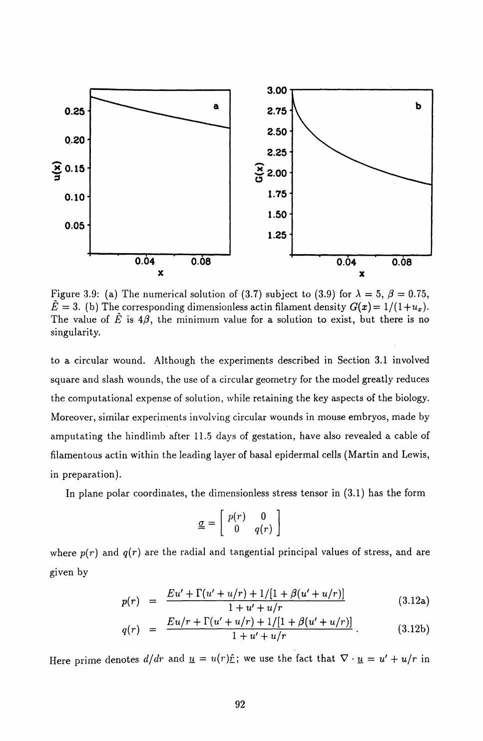
0.25

0.20

3 0.15-a

0.10

0.05

0.04 0.08

§2.00

0.04 0.08

Figure 3.9: (a) The numerical solution of (3.7) subject to (3.9) for A = 5, j3 = 0.75, E = 3. (b) The corresponding dimensionless actin filament density G(x)= l/(l+wz )- The value of E is 4/3, the minimum value for a solution to exist, but there is no singularity.

to a circular wound. Although the experiments described in Section 3.1 involved

square and slash wounds, the use of a circular geometry for the model greatly reduces

the computational expense of solution, while retaining the key aspects of the biology.

Moreover, similar experiments involving circular wounds in mouse embryos, made by

amputating the hindlimb after 11.5 days of gestation, have also revealed a cable of

filamentous actin within the leading layer of basal epidermal cells (Martin and Lewis,

in preparation).

In plane polar coordinates, the dimensionless stress tensor in (3.1) has the form

cr = p(r) 0 0 q(r)

where p(r) and q(r) are the radial and tangential principal values of stress, and are

given by

Eu' + r(w' + u/r) -f 1/[1 -f f3(u' + u/r)]p(r) =

q(r) =

1 -f u' + u/r Eu/r + T(i/ + u/r) + 1/[1 + j3(u' + u/r)]

1 + u' -f u/r

(3.12a)

(3.12b)

Here prime denotes d/dr and u = u(r)r ; we use the fact that V • u = u' -f u/r in

92

radially symmetric plane polar coordinates. Thus

dr r r 00 r 80

r (3.13)

using the relations

Substituting the forms for p(r) and q(r) in (3.12) into (3.13) gives

~~ ar'Eu' + r( / ' 1 / ^

1 1 --\-T 1 / / V*

1 +

) + !/[! 4u1 + u/r

• P(u' Hhu/r)]" E u' — u/r r 1 + u' + u/r

Thus the dimensionless governing equation (3.4) in this geometry is

drEu' + T(u' + u/r) + 1/[1 + /3(u' + u/r)]

1 -f u' + u/ru' — u/r rXu

1 + u' 4- w/r 1 4- w 7 4- w/r(3.14)

We take L, the length scale used in the nondimensionalization, to be the wound

radius, so that the boundary conditions are

(3.15a)

(3.15b)

+ !/[!+ /?(</ + u/r)] = 0 at r = 1

u = 0 atr = oo.

Throughout the remainder of this chapter and Chapter 4, we consider wounds of

radius 500//m; all the wounds in the various experiments described above are of

about this length-scale. At the developmental stages we are considering, a typical

cell diameter is about lO^m, so that the dimensionless cell length is about 0.02.

3.4.1 Solutions with constant tractionWe begin by considering solutions of equation (3.14) subject to (3.15) with constant

traction stress per actin filament, so that /? = 0. This is the form taken by Murray

93

and Oster (1984) in the first continuum model of epithelial morphogenesis. Equa­ tion (3.14) is then

Eu' + T(uf + u/r) + 11 + u' + u/r

r u' — u/r1 + u' + u/r

rAu1 + u7 + u/rdr

For algebraic simplicity, we assume that F ^ 1, and write

(3.16)

(3.17)

It is highly unlikely that a specific value of a parameter such as F = 1 would ever arise in a biological situation, so that the constraint F -^ 1 is biologically acceptable. Moreover, we show below that a solution of the required form does not exist when F > 1. This change of parameters simplifies the equation since the dimensionless parameter T appears only in the boundary condition at r = 1. In terms of these new parameters, equation (3.16) is

d Eu' + 11 -f u7 + u/r

m * m

E(u'-1+u'H

u/r)- u/r

rAu1 + u' + u/r

that is rEu" (1 +„' + -)- r (EU' + l) L" + - - ±\ \ r j \ / y r r2 J

which reduces tour

u rAu(l.+ u' + u/r) ~~~ Eu + r(E-l)r2 (3.18)

The boundary condition (3.15a) is in this case

u = — (3.19)

Recall that in one dimension for the case of constant traction, that is (3 = 0, a necessary and sufficient condition for a solution of the required form to exist is that E+T > 1. In the case F < 1, we now show that this is also a necessary condition in the radially symmetric geometry. When F<l,jE + F>lif and only if E > 1. Suppose that on the contrary E < 1. Then since u(oo) = 0, and u and 1 - A = (1+ u' + u/r) are positive for all r, the right-hand side of equation (3.18) is negative for sufficiently

94

large r, since all the terms are positive except for r(E — 1). The requirement that this

right-hand side must always be finite thus implies by continuity that for all r > 1

„ u' u d ,_ . 0 > u" + - - - = — V • u .

r r* dr

But as r —> oo, V-w —»• 0. Thus V-w > 0 for all r > 1. However, we look for a solution

in which V • u < 0 everywhere. Thus we require E > I for a solution of the required

form to exist. But if E = 1 equation (3.18) can easily be solved analytically. This

is done in Section 3.5, and the solution, given in (3.24), cannot satisfy the condition

u(oo) = 0. Thus for F < 1, the strict condition (E-\-T) > 1 is necessary for a solution

of the required form to exist. Numerical solutions suggest that it is also sufficient,

and that the solution is unique.

In Section 3.5 we discuss the possibility of finding a uniformly valid asymptotic

approximation to the solution of (3.18) subject to (3.19) and (3.15b) using singular

perturbation theory. Here we consider numerical solutions and their relationship to

the experimental observations described above.

We have successfully used two methods of numerical solution, which we now

discuss. The first was a shooting method, in which we treated (3.18) subject to

(3.19) as a nonlinear algebraic equation, with u(l) as the unknown and u(oo) as the

function of u(l) that was to be set to zero. We solved for the value of w(l) such

that w^oo) = 0, starting arbitrarily with r^ = 3, and gradually increasing r^ until

the effect of further increase on the solution near the wound edge was negligible; the

ordinary differential equation was integrated using a Runge-Kutta-Merson method.

We found this method to be successful provided (E — 1) was not too small. The

reason for the numerical difficulties as E decreases to 1 is that the problem is not

well posed as an initial value problem. For, if u(l) = u0 is the required initial value

such that u(oo) = 0, then a necessary condition for the initial value problem to be

well posed is that the solution u (r) is Lipschitz continuous in WQ, that is that for some

positive constant kL and for sufficiently small 6,

u(r) \u(i)=u0 +6 ~u(r) \ u (i)=u0 < kL 6 for all r > 1 .

95

Figure 3.10: Numerical solutions of (3.18) as an initial value problem, with the three initial conditions u(l) = u0 , u0 • (1 ± 2.5 x 10~3 ); u'(l) is calculated from (3.19), and the equation is integrated using a Runge-Kutta-Merson method. Here u0 is the required initial value such that w(oo) = 0; the parameter values are T = 20, E = 1.03 and A = 4. The rapid divergence of the solutions in the region r > 1.7 illustrates that equation (3.18) is not well posed as an initial value problem because the solution is not Lipschitz continuous in u0 .

Numerical solutions indicate that this is definitely not satisfied: Figure 3.10 shows

the effect of a ±0.25% change in w(l) relative to u(l) = u0 , for E = 1.03, T = 20 and

A = 4. In this figure, the solutions diverge in the neighbourhood of r = 1.7, and this

is also the case for perturbations in the solution at r = 1.2, 1.4 and 1.6 (numerical

solutions not shown). It is unclear from a superficial inspection of equation (3.18)

why this region should be problematic, but the singular perturbation analysis in

Section 3.5 shows that it is simply the intermediate layer (see page 102).

The second method of numerical solution used deferred correction and Newton

iteration. We solved (3.18) as a boundary value problem on [1,^], subject to (3.19)

and u(roo) = 0, with ?\x> chosen sufficiently large that increasing its value had a neg­

ligible effect on the solution near the wound edge. We found that r^ = 5 was an

appropriate value. We used a nonuniform initial space mesh based on the layered

nature of the solution discussed in Section 3.5. Successful implementation of this

method required a reasonable initial approximation to the solution, and we found two

96

Figure 3.11: Numerical solutions of equation (3.18) subject to 3.19 and (3.15b) for E = 1 + 0.04 x 2~ n , n = 0,1,... ,6. The other parameter values are T = 20 and A = 4. The convergence of these solutions as (E — 1) is successively halved justifies the continuation method used to obtain numerical solutions for values of E close to 1.

ways of obtaining such an approximation. The first was to use the leading order uni­

formly valid composite expansion obtained using perturbation theory in Section 3.5

and given in equation (3.32). The second, which enabled numerical solutions to be>v

obtained for small values of (E — 1) without appealing to the analysis of Section 3.5,

was to obtain the solution for a larger value of E using the shooting method, and to-V **>

then use continuation in (E — 1) to obtain the solution for the required value of E.

That is, we successively halved (£ —1), and solved (3.18) using the deferred correction

technique, with the solution for the previous value of E as the initial approximation.

The convergence of the solutions as (E — 1) is successively halved is illustrated in

Figure 3.11. We found this deferred correction method to be extremely successful,

especially when using (3.32) as the initial approximation.

As in Section 3.3, we look for the model solutions to capture not only the phe­

nomenon of the actin cable at the wound edge, but also the extent to which the various

cell layers retract in response to wounding. Although it is difficult to be very precise,

in experiments involving circular wounds in mouse embryos made by amputating the

97

v^>9

0.10

0.08

0.06

0.04

0.02

a

1.04 1.08

7-

6-

5-

3-

2

1.04 1.08

Figure 3.12: (a) The solution of equation (3.18) subject to (3.19) and (3.15b) for A = 40, E = 1.1 and T = 0.5. (b) The corresponding dimensionless actin density G(r) = 1/(1 + V • «)• The solution captures the superficial aspects of the response to wounding observed experimentally, but fails to capture the phenomenon of the actin cable.

hindlimb bud after 11.5 days of gestation (Martin and Lewis, in preparation), a re­

traction of the wound edges by about 10-15% of the wound radius is observed, with

only the leading 4-5 cell layers significantly contracted.

The model solutions were able to capture these more superficial aspects of the

response to wounding, as illustrated in Figure 3.12. Crucially, (E — I) must be

small and positive to capture such behaviour. Since there are only three unknown

parameter values, an extensive parameter search is possible. However, in the course of

such a search we were unable to capture the intense aggregation of actin at the wound

edge that constitutes the actin cable. The band of aggregated actin in Figure 3.12

spans several cell lengths. (Recall that the dimensionless cell length is about 0.02).

We conclude our investigation of solutions with 0 — 0 by considering the case of

r > 1, in which case E, T and A are negative. This parameter domain includes the

case of a rubber sheet, which is given by putting TO = 0. However, with E, T and A

negative we were unable to capture even the overall features of the initial response to

wounding, that is we were unable to find solutions in which w(l) was between about

0.1 and 0.15, with u decreasing rapidly over a dimensionless length scale of about

98

0.1. This numerical investigation suggests that F < 1 is a necessary condition for a

solution of the required form to exist.

3.4.2 Solutions with variable tractionWe now consider the solutions of the model equation in a radially symmetric two-

dimensional geometry with /? > 0, so that there is actin filament synergy in cell

traction forces. Expanding equation (3.14) then gives

r[F - Eu'](u"+ - - ^} + rEu" (I + u' + -) + E (u' - -} ( 1 + u' + -) \ r r2 / \ r) \ r)\ r)

r (u" + u'/r — u/r2 ) 1 + @(u' + u/r) 1 + (3(u' + u/r)

= Xru I 1 + u' + -} . (3.20) r/

For notational simplicity, we write henceforth

Ti(r,u,u) = 11 -f /3(u' + u/r) 1 -f + u/r)

+ 1 -r.

Equation (3.20) then simplifies to give

u7

u Xru ( l" Eu + r(E -

We solved equation (3.21) subject to the boundary conditions (3.15) numerically,

using deferred correction and Newton iteration with continuation in /?. Methods of

numerical solution when 0 = 0, the case of constant traction, were discussed above.

Using this solution as a starting point, we gradually increased the value of /?, using

the solution for the previous value as the initial approximation. As expected from the

one-dimensional equations investigated in Section 3.3, there appeared to be a critical

value of /?, dependent on the other three parameters, above which solutions could not

be obtained. Throughout the wide range of parameter values we have considered,

this critical upper limit was lower in this new geometry than in one space dimension.

In contrast to the case of constant traction considered above, as j3 approached its

critical upper limit, the band of aggregated actin at the wound edge in the model

solutions became much sharper, to such an extent that it was localized within the

leading cell layer. Such a solution is illustrated in Figure 3.13. However, in this

99

0.090.08

0.07

0.06

£0.05

* 0.04

0.030.02

0.01

1.02 1.04 1.06 1.08 1.10 r

1.02 1.04 1.06 1.08 1.10r

Figure 3.13: (a) The solution of equation (3.21) subject to (3.15) for A = 3.0, E = 0.5, F = 0.8, and (3 = 0.255. (b) The corresponding dimensionless actin filament density G(r) = 1/(1 + V • u). The band of aggregated actin at the wound edge (r = 1) is sharp enough to correspond to the actin cable observed experimentally.

solution, the derivative du/dr is less than —1. Moreover, this was true in all solutions

which captured the phenomenon of the actin cable. Note that since the actin density

at the wound edge is (7(1) = 1/[1 + w'(l) 4- "(I)] and u(l) > 0, large (7(1) requires

u'(l) < — 1. In such a solution, the dilation is still greater than —1. However, the

biological implication of u'(l) < —1 is that cell layers near the wound edge 'change

places' after wounding, so that the leading cell layer prior to wounding does not

remain the leading cell layer after wounding. Such a phenomenon is certainly not

observed experimentally. This inadequacy in the model predictions occurs because

the approximation A = —V • w, which was introduced on page 78, breaks down

as du/dr approaches — 1. In the next chapter we consider an improved form of the

model in which we use a more accurate representation of the local compaction A. We

conclude this chapter by deriving an approximate solution of equation (3.18) subject

to (3.19) and (3.15b) using singular perturbation theory.

100

3.5 Singular Perturbation Analysis of the Case of Constant Traction

We have shown that for the solution of equation (3.18) subject to the boundary condi­

tions (3.15) to capture the cell retraction aspects of the initial response to wounding,

it is necessary that (E — 1) is small. In this section we exploit this fact, and look for

a uniformly valid asymptotic approximation to this solution using singular perturba­

tion theory. Such methods are clearly surveyed in the book by Kevorkian and Cole

(1985). In this section we write e = (E — 1), and for notational simplicity we drop

the tilde on the parameter A. With this notation, equation (3.18) is

„ u' u _ ArM(l + u/r + u'} r r2 (1 -f e)u -f er

and the boundary conditions (3.15) have the form

u'(l) = - (3.23a)

ti(oo) = 0. (3.23b)

We begin by attempting to solve equation (3.22) subject to (3.23) when e = 0.

This is a linear problem which integrates immediately to give

u' — u(\r — 1/r) = Ar2 /2 + constant.

The integrating factor here is r exp(—Ar2 /2), which gives the general solution of (3.22)

when e = 0 as

u = — — - -f — exp[A(r2 — l)/2] (3.24)

where A and B are constants of integration.

This solution does not satisfy w(oo) = 0 for any values of A and B, so that the

problem is singular as e —» 0. Imposing the condition (3.23a) gives a solution MO of

the form

fi0 = I (- - r] + - {\(T + !)-!+ exp[A(r2 - l)/2]} . (3.25) & \ i / I

This solution is plotted in Figure 3.14 for a range of values of B. We use parameter

values A = 4 and T = 20 in this figure, rather than the values A = 40, T = 0.5 used in

101

-0.25

-0.50Figure 3.14: The solution (3.25) of equation (3.18), for ten evenly spaced values of the constant of integration 5, between 0.0023 and 0.0155. The parameter values are A = 4 and T = 20.

the solutions in Figure 3.12 which capture the overall features of the initial response

to wounding. This is also done in the other figures in this section, and is for reasons

of clarity, as explained below.

3.5.1 Possible rescalingsWe look for a rescaling that will capture the behaviour of the solution of (3.22) subject

to (3.23) for large r. Such a rescaling has the general form r = /i(e)r, u = u/£(e),

with fi(e) — 0(1), £(e) = ^(1) anc^ /i • ^ = o(l) as e —> 0. Here, as usual, the notation

f(e) = 0(1) includes the case f(e) = o(l); the condition [L • v = o(l) ensures that we

do have a genuine rescaling. This gives

d2 u 1 du uI Art ' A t A Artdr2 r dr r 2- er] = Xru

*•*

T rt* I*— dr

All the terms in this equation are o(l) except Xru. Thus w| e=0 = 0, and similarly all

terms in any asymptotic expansion for u are zero.

Therefore we have to introduce a layer rescaling to give a solution intermediate

between this zero solution at large r and the regular solution (3.25) near r = 1.

The general form of the variables in such a layer is r* = (r - fl)//i(e), u* = u/i/(c),

where fjt(e) = 0(1) and i/(t) = 0(1) as e -* 0. Here r = R is the centre of the layer.

102

Substituting into (3.22) gives

R

which to leading order is

~ vu* + eR

all the other terms can certainly be neglected to leading order. There are then a

number of possibilities, according to the orders chosen for // and v\

(a) ft2 ~ v ~ e. This is discussed in detail below.

(b) // 2 ~ v ;> e. Then d2 u* /dr*"2 = A/? to leading order; the parabolic layer solution

cannot match the zero solution to the right of the layer.

(c) fi 2 ~ e ^> */. Here to leading order d2 u*/dr*2 = Aw", =^ w* a exp(— x/Ar*) since

u*(oo) = 0. This exponential solution cannot be matched to the left of the

layer.

(d) ^2 ^> v and /j 2 ^> e. In this case all terms in any asymptotic expansion for u*

are zero.

(e) // 2 <C ^ or f.i 2 <C e. Here d2 u*/dr*2 = 0 to leading order; the linear solution

cannot match the zero solution to the right of the layer.

Thus the only rescaling that can give an appropriate layer solution is (a), namely

u* = u/e, r* = (r - R)/\/e. Multiplying (3.26) by du*/dr* and integrating gives

I(111L) = X R2 I ^ - log (1 + ~ ) I + constant. 2 \dr* J iR \ /t/J

Imposing u* — 0 at r* = oo shows that the leading order term in the layer solution

is then

ut = R- H~ l (C - r*\/2A) where #(f) = J* [8 - log(l + 6)}~ 1/2 dO ,

and where C is a constant of integration.

103

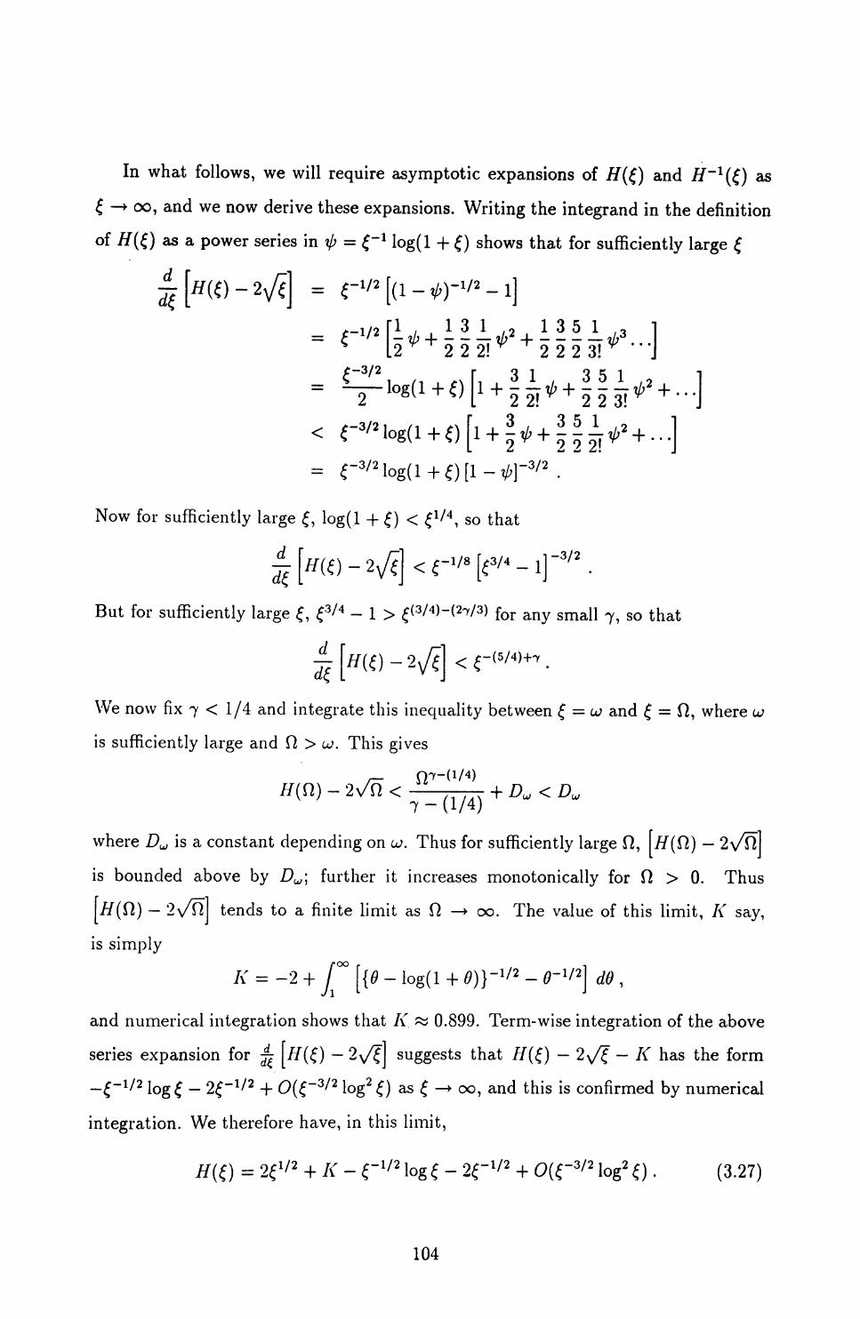
In what follows, we will require asymptotic expansions of H(£) and H~l (£) as -> oo, and we now derive these expansions. Writing the integrand in the definition

of H(£) as a power series in \j> = £~ l log(l 4 £) shows that for sufficiently large

= r'/2 [a -,_!/, fl . ,1 3 1 , 2 1 35 1 ,3 1= * ' l2* + 222!* + 2223!* -J

Now for sufficiently large £, log(l 4 £) < £ x /4 , so that

£-1/8

But for sufficiently large (, <f3/4 - 1 > £(3/4)-(27/3) for any small ^ SQ that

<

We now fix 7 < 1/4 and integrate this inequality between £ = u and £ = 0, where a;

is sufficiently large and 17 > a;. This gives

W

where .Du, is a constant depending on w. Thus for sufficiently large 0,

is bounded above by Du ', further it increases monotonically for 0 > 0. Thus

/f(i7) — 2\/iT tends to a finite limit as 17 — > oo. The value of this limit, K say,

is simplyK = -2 + ^°° [{0 - log(l + 0)}~ 1/2 - r1 /2] dB ,

and numerical integration shows that K. % 0.899. Term-wise integration of the above

series expansion for ^ [#(f ) - 2>/f] suggests that //"(^) - 2^ - A" has the form

— £ -1 /2 logf — 2£~ 1 /2 4- (9(^~3/2 log2 <f) as ^ — »• oo, and this is confirmed by numerical

integration. We therefore have, in this limit,

= 2f 1/2 + K - r1/2 log c - 2r1/2 + o(r3/2 log2 o - (3.2?)

104

From this, it is clear that to leading order, H~l (x) = (x — K)2 /± as x —> oo.

Substituting H~ 1 (x) = (x - /O2/4 + y(x) into (3.27) and expanding for large x

implies that

1x = + K

~3/2

= (x-K){\

2 1-2(x -

2K K2X X'

8y 5

x — K

(s-/02 (a; -

01 on i o\ , , y - 2 log x - 2(1 - log 2) + —— +x

Therefore as x —> oo

[log{j(x-

2 log z + 2(1 -log 2)

+ O(x~* log2 x

X'

(x "/)2 +21og>T + 2(l-log2)-^ + of- 4 a; \x,

(3.28)

3.5.2 Matching to leading orderMatching to the right of the layer is guaranteed by the boundary condition at r* = oo.

For matching to the left of the layer we use an intermediate variable r^ = (r — #)/7/(e),

with Y/C <C rf(e) <C 1, and consider the behaviour of the left-hand and layer solutions

as e —> 0 with rn fixed. Then r —* R and r* —* —oo. Now (3.28) implies that

, A^?°~T r /c - c]+ V/2A .

-f 0(r*) as r* —>• —oo. (3.29)

Matching to leading order therefore requires

M-,

105

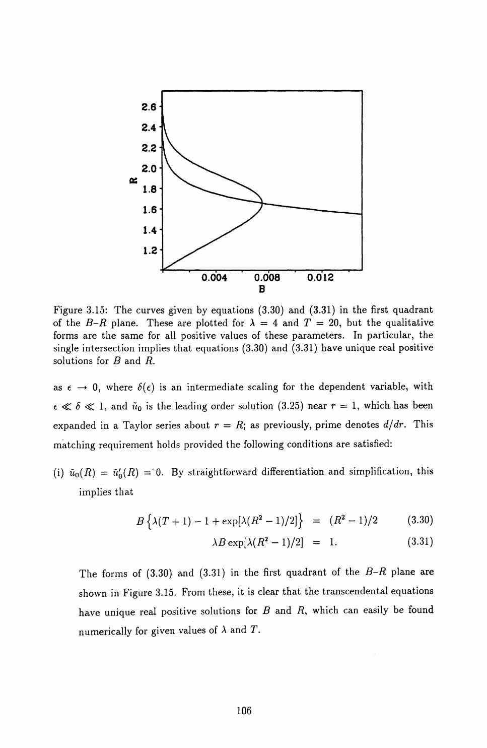
Figure 3.15: The curves given by equations (3.30) and (3.31) in the first quadrant of the B-R plane. These are plotted for A = 4 and T = 20, but the qualitative forms are the same for all positive values of these parameters. In particular, the single intersection implies that equations (3.30) and (3.31) have unique real positive solutions for B and R.

as e —> 0, where S(e) is an intermediate scaling for the dependent variable, with

e <C 6 < 1, and u0 is the leading order solution (3.25) near r = 1, which has been

expanded in a Taylor series about r = R\ as previously, prime denotes d/dr. This

matching requirement holds provided the following conditions are satisfied:

(i) uQ (R) = u'0 (R) ="0. By straightforward differentiation and simplification, this

implies that

£{A(r+l)-l+exP [A(#2 -l)/2]} = (R2 - l)/2 (3.30)

A£exp[A(#2 -l)/2] = 1. (3.31)

The forms of (3.30) and (3.31) in the first quadrant of the B-R plane are

shown in Figure 3.15. From these, it is clear that the transcendental equations

have unique real positive solutions for B and R, which can easily be found

numerically for given values of A and T.

106

(ii) UQ(R) = A./?, which we now prove:

\B - — exp[A(fl2 -

= Afl,

using (3.30) and (3.31).

(Hi) T/ 3 < 6.

(iv) T/CTJ = O(6). If we further specify v/er/ < £, then C is not determined by the

leading order matching. However, the absence of a ^/e term in the expansion

near r = 1 (see below) requires that C = K.

Thus we have obtained matched asymptotic expansions to leading order for the

solution of (3.22) subject to (3.23). We obtain a composite expansion in the usual

way, as "outer solution + inner solution — common part" (see, for example, Murray,

1984; Kevorkian and Cole, 1985). This gives

7/ _ r < R Ucompo(r) ~ eu*r* r>R.

Figure 3.16 shows UQ, ewo> ucompo and the numerical solution of (3.22) subject to

(3.23), plotted against r, for t = 0.03 and 0.003. The difference between ucompQ and

UQ decreases to zero as r decreases below 1. This figure demonstrates very clearly

that the problem is singular as e — > 0: the numerical solutions of the full system

are quite different in parts (a) and (b) of Figure 3.16, despite c being very small in

both cases. Moreover, the difference between these numerical solutions and UQ, the

solution for e = 0 subject only to boundary condition (3.23a), is very considerable

even for t = 0.003. In Figure 3.16, we use parameter values A = 4 and T = 20 rather

than the values A = 40, T — 0.5 used in the solutions in Figure 3.12, which capture

the overall features of the initial response to wounding. We do this for reasons of

clarity: as A increases and T decreases, R decreases towards 1, and at A = 40 and

T = 0.5 R ~ 1.08. The analysis is of course valid for all parameter values.

107

1.2 1.4 1.6 1.8 2.0 Radius, r

1.4 1.6 1.8 2.0 Radius, r

Figure 3.16: Plots of the regular solution, WQ(^), the leading order layer solution, euo(r*), the leading order composite solution, ucomp0 (r), and the numerical solution of (3.22) subject to (3.23), against r, for (a) e = 0.03 and (b) e = 0.003, with A = 4 and T = 20. The numerical solutions were obtained using Newton iteration and deferred correction, with ucompo(r) as the initial approximation. To indicate the layer regions, the lines r — R and r = R ± y/c are drawn. The error in the leading order composite solution appears to be 0(y/e), and this is confirmed by our investigation of the higher order terms.

3.5.3 Higher order correctionsThe leading order composite solution differs significantly from the numerical solution of (3.22) subject to (3.23) even for values of the parameter e as small as 0.03. We

now consider higher order corrections to the leading order approximation obtained above. The full equation for u* contains ^Jt terms, so that the first order correction

to UQ is O(y/c). Substituting u* = UQ + \Jlu\ in the full equation for u* and equating

coefficients of ^/e gives\R2

(*5 + Wu*r*

+ R 0

RdrNow Wo( r*) ls monotonically decreasing, so we can use UQ as the independent variable;

this is feasible since duQ/dr* andf WnM d2 u* Run du* R21 4- -^H

are known functions of UQ. We then have

2R2 l=* -~Rji du*02 + tiS + /2rft«S

^S5 +

R dr* (3.33)

108

subject to u\ = 0 at UQ = 0. Here we use the identities

du\ = du^du^ d2u\ (Put du\dr* ~ dr* du*Q an c/r*2 ~ dr** du% \dr

The homogeneous equation corresponding to (3.33) can be integrated directly, giving

linearly independent solutions

1 /2?/*i-a*

-

where /(£) = fi{0 - log(l + 0)}~3/2d9. The inhomogeneous equation can thus be

solved using the method of undetermined coefficients, that is, we look for a solution

of the form

subject to the constraint

da\ . „. da-i ... T^/iK +T^K =0

Substituting this into (3.33) gives linear equations for dai/duQ and da^/du^. Solving

these gives the general solution of (3.33) as

+ A + , (3.34)

where F(UQ/R) is the right-hand side of (3.33), and PI and Qi are constants of

integration. F is integrable near zero, since straightforward series expansion shows

that as £ -» 0, F(£) = f/\A + O(^2 logf )• Expanding the integral /(f) for small f

shows that as u*Q -* 0 (so that r m -* oo), «; = -QifS^Wo' 1 + 5)/6 + o(l), and thus

the boundary condition at UQ = 0 requires the constant of integration Qi to be zero.

109

For the purposes of matching, it is the behaviour of u\ as wj —» oo (so that

r* —* — oo) that is of interest. Expanding for large £ gives

) r1/2]2) r1/2

where 1^ = Iim4_+00 /(<f). Here we have used the expansion (3.27) of H(() for large

£. Integrating term-wise and substituting into (3.34) suggests that as UQ —»• oo,

6 Ru i = ~ 3/2

.\/2A 6

*.l/2'o \ ). (3.35)

Here the constant U^ is dependent on the outstanding constant of integration

PI log R 16f V/2A,

These results are confirmed by numerical integration.

Consider now higher order corrections to UQ. Substituting u

and (3.23), and equating coefficients of ^/e, gives

12 \/2A

in (3.22)

«',' + — — — = Xr ( — + u( } 1 r r2 V r V

(3.36)

subject to u((l) = —Titi(l)/(T -f- 1), where as previously, prime denotes d/dr. This

can be solved in the same way as (3.25) was obtained, giving

{tl = ^i {AT + A - 1 + exp[A(r2 - l)/2]}

where BI is a constant of integration. Now matching even to O(-y/e) clearly requires

wj(/?) = 0, so that BI = 0 and thus HI = 0.

We therefore look for a 0(e) correction to u0 . Substituting u = u0 + eu2 in (3.22)

and (3.23), and equating coefficients of e, gives

fij + (I - Ar) fi'a - (A + £) fi a = -^(fio + r) (l + ^ + fii) (3.37)

110

subject to w'2 (l) = ~[Tu2(l) + u'Q(\)\/(T + 1). This equation can again be solved using the method of undetermined coefficients: the homogeneous equation has linearly independent solutions 1/r and eAr2/2/r. This gives

S2 (r) = gl {AT + A - 1 + exp[A(r2 - l)/2]} - l + *TB +

(3 '38)2Bexp[A(U -l)/2] , Au/2 "

where D = 1 + 2B(\T + A — 1) and B2 is a constant of integration. For the purposes of matching, it is the behaviour of this solution as r — * R~ that is of interest.

This can be obtained directly by series expansion, but the algebra required is rather

involved. Instead, we derive the behaviour of the solution in this limit directly from

the differential equation (3.37). Expanding the coefficients as power series in £ = r— R gives

f *[(*Let U2,iead be the solution of the equation given by taking only the leading order term

of each coefficient in (3.39), so that

, . -- + UVead = ~' ( ]The corresponding homogeneous equation has linearly independent solutions ea+<*

and ea~^ where a± are the roots of the characteristic equation. Using the method

of undetermined coefficients, we therefore look for a solution of the form

= a+ (C) exp[a+C] + «"(C) exp[a~C] , (3.41)

where the unknown functions a± (C) are constrained to satisfy

+ exp[a-C] = 0. (3.42)

Substituting (3.41) into (3.40) and using (3.42) gives

da* 2R I

Ill

But

/ ex dx ex_ ____ ___ _ __ |

T* « T*»*/ t*/

X X2 X31 I I •«/ U/log N + Y7 + 272! +

(see, for example, Beyer, 1981). Using this expansion and (3.41), the general solution

of (3.40) is

og |C| + O((* log |C|) + A+e*< + Aje"'< (3.43)

as ( — * 0, where A* are constants of integration.

Denoting the correction to this leading order solution by U2,corr(r) and substituting

HI = U2,iead + u^corr into (3.39) implies that to leading order as £ — » 0, U2,corr satisfies

I , D\ rfu 2 .corr /\ , 1 \ - 4A/t!2 + 12" A/V -3T" ~ vA + &) U2 'corr = — sT"'This can again be solved using the method of undetermined coefficients, and the

solution has the form

= -4(1 + A#2 /3)C log |f | + O((* log |f |) + A+ea < + Ajea"c (3.44)

as (" —•* 0, where ^3 are constants of integration. Since we require U2,iead ^ ^2,corr

as (" —> 0, A% = A^ = 0. Adding the two solutions (3.43) and (3.44) implies that as

u2 = 2R log |C| + U2 + (I\R2 - 6) C log |C| + C/2 ,iC + O [C log |Cl] (3.45)

where f/2 ls an outstanding constant of integration, the value of which determines

the constant B2 in (3.38), and thus f/2| i- This expansion is confirmed by numerical

integration.

3.5.4 Intermediate terms and conclusionsComparison of the expansions (3.35), (3.45) and the leading order expansions in

Section 3.5.2 indicates that a number of terms remain unmatched at the left of the

layer, even to 0(\/e). We found that in order to complete the process of matching

to higher order it was necessary to introduce logarithmic terms between the leading

112

and higher order terms found previously, in both the left-hand and layer solutions.

Specifically, we introduce a term elogeu/(r) in the left-hand solution and a term

Y/elogeujf^r*) in the layer solution.

Substituting u = u0 + e log t u\ in (3.22) and (3.23) and equating coefficients of

elogc shows that u\ satisfies the same equation (3.36) and boundary condition as u\.

Thus

u\ = — [\T + A - 1 + exp[A(r2 - l)/2]} (3.46)

where B\ is a constant of integration.

The equation satisfied by u* is obtained in the same way; using UQ as the inde­

pendent variable, as in Section 3.5.3, gives

u duR

= 0

subject to u* = 0 at UQ = 0. This equation can be solved by integrating once,

multiplying by the integrating factor {UQ/ R + log(l + UQ/R)}~3/2 and integrating

again, giving the general solution as

11*|-where C*i, Ci are constants of integration. Straightforward series expansion shows

that the behaviour of this solution as UQ — > 0 (so that r* — > oo) is

3

Thus the boundary condition at tij = 0 requires Ci = 0, so that as uj —+ oo (so that

-oo),

(3.47)

We can now consider matching the amended left-hand and layer solutions: as in

Section 3.5.2, matching to the right of the layer is trivially satisfied. Using (3.35),

(3.45), (3.47) and the leading order expansions in Section 3.5.2, and expanding (3.46)

in a Taylor series about r = R, the condition for matching to O(^/e) is

113

Utf - 6)

log(A/2)] + O - C/v/A/2

log v)

log

(3.48)

as e -» 0, where V\ = BI {XT + A - 1 + exp[A(#2 - l)/2]} //2. Here we have obtained higher order terms in the behaviour of «J as r* — »• — oo, using (3.28). Simplifying the expression for u'o(R), using (3.3) and (3.4), shows that u'o(R) = \2 R2 . Thus the matching condition determines the outstanding constants of integration as follows:

= R[2 + log(A/2)]

- 3 - - 1)]

We then have matching to 0(>/e) provided the following conditions are satisfied by

6(e) and 7/(e) as e — » 0:

(a) r/ 4 = o

(d) c = o(r]8)

(b) rj 2 ^/c\ogc = 0(8)

(e) e3/2 log e log 77 =

(c) Tj 2 ^/clogr) = 0(8)

(f) elog2 77 = o(

Trivially (d)=>(f). Moreover, 77 > ^/e, so that log 77 = O(loge); thus (b)=»(c) and (d)=^(e). Also, 8 ^> e ^> e3/2 log2 e, and multiplying (a) by this result implies (b). Thus for matching to 0(\/e) it is necessary and sufficient that 7/ 4 <C \/c8 and e <C ^V- These conditions can be portrayed graphically if we consider only orders of magnitude that are powers of e: intermediate orders involving logarithms need not concern us. Thus, we write 8 = Os (ep ), rj = Os (eq ), where, as usual, the notation / = O3 (g) means that / = 0(g) and / ^ o(g). The two conditions are then 4qr > p + 1/2 and p + q < 1. We also require q < 1/2; the conditions T;3 < 8 and ^/erj = O(8) for leading order matching are implied by (a) and (d). The p-q domain such that

114

o IIp

*cf

1/8 1/2p, where <5=0s(ep)

1/4 1/2p, where <5=0s (c p)

Figure 3.17: The domain of orders of magnitude of 8 and 77 for the matching condition (3.48) to be satisfied. We are considering only orders of magnitude that are powers of e, with 8 = 0s (ep ), r? = Os (cq ). The shaded region is the p-q domain such that the matching condition is satisfied, (a) for matching to O(v^), and (b) for matching to 0(c).

these conditions are satisfied is illustrated in Figure 3.17a. For matching to 0(e), the corresponding conditions are 4q > p + 1 and p + q < 1/2, and the p-q domain in this case is illustrated in Figure 3.17b. The corresponding p-q domain exists, so that matching is possible, to any order that is > e6/5 .

We obtain a higher order composite expansion as in Section 3.5.2, giving

f elogew/(r) -\

V / —log e - 2/fc log |C| - #[2 + MA/2)]e

r < R

log cu? (r.) + eut(r*) r > R . where C = r - R. Figure 3.18 shows t/ compi, ucomp0 and the numerical solution of (3.22) subject to (3.23), plotted against r, for e =.0.03. The higher order corrections dramatically improve the quality of the composite expansion as an approximation to

the exact solution.In addition to being an interesting problem in singular perturbation theory, the

115

1.0

0.8

§ 0.6E0)oJO

.2 0.4Q

0.2

* Leading* .order '.comp so In

Higher ' order comp soln

Num soln

1.2 1.4 1.6 Radius, r

Figure 3.18: Plots of the leading order composite solution ucompo(r), the higher order composite solution ucomp\(r) and the numerical solution of (3.22) subject to (3.23), against r, for € = 0.03, A = 4, T = 20. The numerical solution was obtained using Newton iteration and deferred correction, with ucompo(r) as the initial approximation. To indicate the layer regions, the lines r = R and r = R ± y/e are drawn.

good analytic approximation to the solution given by this higher order composite

expansion served two purposes. Firstly, it increased our understanding of the struc­

ture of this solution. In particular, the layer structure of the solution enabled us to

understand various difficulties experienced in solving equation (3.22) numerically, as

explained on page 96. Secondly, it provided a crucial first approximation in numerical

solutions of the more biologically relevant improved model, as discussed in the next

chapter.

116

Chapter 4

Extending the Model: the Formation of the Actin Cable

4.1 The Need for an Improved ModelIn the previous chapter, we developed and analysed a basic model for the initial re­

sponse of embryonic epidermis to wounding. The one-dimensional solutions compare

well with experimental observations. However, numerical solutions of the model equa­

tions in a radially symmetric geometry indicate that changes are required in these

equations. Specifically, as explained in Section 3.4.2, the approximation A » - V • u

must be improved. Here A is the fraction of the pre-wounding volume by which

a small region of cytogel contracts in the initial response to wounding. Now when

the sides of an infinitesimal rectangle are oriented along the principal axes of the lo­

cal two-dimensional strain tensor £, a deformation changes the rectangle into another

rectangle. Therefore, the full expression for A is l-(l+pi)(l+p2 ), where pi and p2 are

the principal values of the local two-dimensional strain tensor g (Segel,

1977a). In the previous chapter we used the approximation A % ~(pi -f p2 ) = -V -u,

following linear elasticity theory. However, this ceases to be a valid approximation

as one of the p^s approaches —1, which occurs in the solutions presented in Sec­

tion 3.4.2. We now consider the model equations with the full form for A, which

in a radially symmetric two-dimensional geometry is A = — (u1 -J- u/r + wu'/r); the

one- dimensional model equations are unchanged, since then only one of the p,-'s is

non-zero. The linear form (3.1) for the stress tensor is still valid (Segel, 1977a), so

that the radial and tangential principal components of stress are now

Eu' + T(u' + u/r) '+ */ I 1 + P(u> + u/r /41 x

1 + u' + u/r 4- uu'/rEu/r + F(u' + u/r) + !/[!+ P(u' + u/r + uu'/r)]

1 + u' + u/r + u

117

these replace p(r) and q(r) respectively in (3.12). Using (3.13), the amended dimen- sionless model equation is therefore

d_ dr

Eu' + T(u' + u/r) u' + t£/r + titi'/r)]1 -f u' + u/r -f uu'/r

, ___ti; — u/r___ _ ____________ 1 + u' + u/r + uu'/r 1 + u' + u/r + uu'/r

Xru

This simplifies to

1(£ + r2 )(r + u) + r(r-tr Xru , u uu 1 -f- u' + - + —

r r

- it' - - n I ^ W /2 WWE ( 1 + - - u'2 + — r r (4.2)

where

T2 = -1

1 + j3(u' +u/r + uu'/r)

The boundary conditions are

/?(1 + M; + u/r + uu' {1 + /?(u' + u/r + uu'/r)} 2

u' + u) 1, ———TT = 0 at r = 1 p(u' + u/r + uu'/r)

u = 0 at r = oo

(4.3a)

(4.3b)

We solved this equation numerically both for ft = 0 (constant traction per actin filament) and (3^0 (variable traction per actin filament). As in Section 3.4.2, we obtained numerical solutions using deferred correction and Newton iteration, with continuation in the parameter 0. As in the one-dimensional equations investigated in Section 3.3 and also the two-dimensional solutions in Section 3.4.2, there appeared to be a critical value of /?, dependent on the other parameters, above which solutions could not be obtained. Moreover, as 0 approached this critical upper limit, the band of aggregated actin became much sharper, so that the model solutions did reflect the phenomenon of the actin cable. However, we were unable to capture both this intense aggregation of filamentous actin at the wound edge and the more superficial aspects of the experimentally observed response to wounding, that is a retraction of the wound edges by 10-15%, with only the leading 4-5 cell layers contracted. A

118

0.061

0.05

^ 0.04 •

3 0.03

0.02

0.01

1.02 1.04 1.06 1.08 1.10r

Figure 4.1: The numerical solution of (4.2) subject to (4.3) as (3 approaches its critical upper limit. The stopping criterion applied to the increase of (3 in the numerical solutions is discussed on page 140. The other parameter values are A = 3.0, E = 0.3, T = 0.8.

typical limiting solution for u(r) as 0 approaches its critical upper limit is illustrated

in Figure 4.1.

Therefore, although the improvement in the representation of the local compaction

A changes the precise form of the model solutions for a given set of parameter values,

comparison of these solutions with experimental data still indicates that improve­

ments are required in the model. A key aspect of the basic model (3.3) is that

the representation of the filamentous actin density is scalar, so that any preferential

alignment of the filaments is neglected. We now reconsider this aspect of the model.

4.2 Stress Alignment of Actin FilamentsThere is considerable evidence in the biological literature that, as illustrated in Fig­

ure 4.2, when a mesh of actin fibres is subjected to a stress field, the fibres tend to

align along the directions of maximum stress. The seminal paper on this topic is

a study involving micromanipulation of fish epidermal cells by Kolega (1986). He

found that in cytoplasm held under tension either by micromanipulation or by the

119

Figure 4.2: A diagrammatic representation of actin filament alignment in response to a non-isotropic stress field. The filaments tend to align along the directions of maximum stress. For clarity we show filaments oriented in two orthogonal directions only, but in the epidermis they are oriented in all directions.

locomotive activity of other cells, actin filaments were aligned parallel to the tension.

Moreover, he found that when the tension was due to micromanipulation, actin fil­

ament alignment occurred within a few seconds, as a direct response to the applied

tension.

In a previous but quite similar study, Chen (1981) applied micromanipulation to

chick heart fibroblasts. His observations of the cytoskeleton suggest that the actin

filament network is like a three-dimensional fish net under tension, oriented along

directions of stress. A similar analogy is used by Kolega (1986). Chen (1981) found

that upon detachment of a fibroblast tail from the substratum, with a consequent

reduction of the stress in the cytoskeleton, the microfilament bundles lost their ori­

entation and reassumed a random meshwork arrangement, over a time scale of about

15 seconds. This rearrangement was a simple reorientation, and not a disassembly

and reassembly of actin filaments.

Valberg and Albertini (1985) exerted forces on pulmonary macrophages from the

lungs of hamsters by causing the macrophages to ingest magnetic particles. They

then applied external magnetic fields, which exerted forces on the magnetic particles

present in the phagosome organelles, and thus on the cell as a whole. They observed

changes in the organization of the actin filament network, resulting in prominent

patches of positive staining for actin coinciding with the location of magnetic particles,

aligned with the magnetic force field. Although not in the authors' conclusions, these

observations suggest alignment of actin filaments along directions of stress.

120

Finally, there is a considerable body of literature on stress-induced alignment

of "stress fibres", that is actin filament bundles, in endothelial cells under shear

stress, which is an important feature of blood flow. The studies by Wechezak tt al.

(1985, 1989) are typical. In these, shear stress was applied to bovine carotid artery

endothelial cells via the steady laminar flow of fluid through a cuboidal channel, one

wall of which was a cell-lined coverslip. The experimental technique is described in

detail by Viggers et al (1986). In the 1985 study, stress was applied to confluent

monolayers. Basal "stress fibres" developed, aligned with the flow direction, that is

the direction of applied stress. This was in contrast to the prominent peripheral rings

of actin filaments in control cells. The 1989 study concerned isolated cells. The "stress

fibre" network reorganized to give a preponderance of actin at proximal (relative to

the flow direction) cell margins. The authors claim that these observations support

those of Kolega (1986). It should be noted that the time scale of the cytoskeletal

reorganization in these studies was several hours, compared to that of a few seconds in

the experiments of Chen (1981) and Kolega (1986). However, the micromanipulation

and flow chamber techniques are very different, with the former unquestionably more

relevant to the epithelial wound situation. Thus we treat the process of actin filament

alignment in response to stress as instantaneous.

Based on the considerable biological evidence for stress alignment of actin fila­

ments, we incorporate such alignment into our model. We are not aware of previous

attempts to incorporate stress alignment of actin filaments into mechanochemical

models of cytogel. This is due in part to the fact that many such models are for­

mulated in a one-dimensional geometry, while filament alignment is an intrinsically

higher-dimensional phenomenon. The reference to filament alignment in Oster and

Odell (1984a) is typical: they simply state that in more than one dimension "more

elastic parameters are required to account for fibre alignment".

We amend our model as follows. In a radially symmetric two-dimensional geom­

etry, the stress tensor £, defined in (3.1), has the form

Sr 0 0 E,

121

where the principal values of stress, Er and £#, are defined in (4.1). To incorporate

filament alignment, we replace this with the form

0cr =0 /(!//>)£, ( '

where p is the ratio of the principal values of the amended stress tensor, that is

p = GrT/vee, and / is a function reflecting the effect of filament alignment on the

mechanical properties of the actin filament network. We are assuming that the actin

filament network exhibits preferential alignment in response to non-isotropic stress,

to an extent which depends on the ratio of the principal values of stress. The result

of this alignment is effective radial and tangential 'components' of actin filament

density, given by Gf(p) and Gf(l/p) respectively, where G is the local 'scalar' actin

filament density. The function / is subject to the following conditions:

(i) /(O) = 0: when the stress is unidirectional, all the filaments are aligned in its

direction.

(ii) /(I) = 1: when the stress is isotropic, there is no preferential alignment of the

filaments.

(iii) f is an increasing function.

In the absence of detailed experimental evidence for the functional form of /, we use

a simple form satisfying these conditions, specifically

/M = (4.5) p + a

where a is a constant, 0 < a < 1. The case a = 0 gives / = 1, that is no preferential

filament alignment. With this form for /, the implicit equation (4.4) can be solved

for the principal values of stress, giving

arr = -^—(Zr-aXe) (4.6a) 1 — a

(fee = ; —— (%0 - a^r) • (4.6b) 1 — a

Equation (4.4) also has solutions in which one of the principal values of stress is

identically zero, with the other non-zero. However, these solutions are unstable to

122

small perturbations in the stress field, such as could arise from movements of the

underlying mesenchyme, and they are therefore not biologically relevant.

For simplicity, we have developed this improved model, which incorporates stress

alignment of actin filaments, in a radially symmetric geometry only. In a more general

two-dimensional geometry, the procedure is as follows. At each point in space, one

must rotate the local coordinate axes so that they are aligned with the principal axes

of the stress tensor g, defined in (3.1). These principal axes are orthogonal since £

is symmetric. In this new coordinate system q_ has the form

cr = Si 00 E2

say. To incorporate filament alignment, we replace this by

00

where crn, <722 are the diagonal entries in this amended stress tensor. Having solved

these implicit equations for <rn and 0*22, one must then rotate the local coordinate axes

back to their original orientations. A key aspect of this procedure is that the 'original'

and 'improved' stress tensor have the same principal axes, though the principal values

are different. In the radially symmetric geometry considered above, this procedureA

is particularly simple since at each point the principal axes of £ are just the r and Q_

axes. Application of filament alignment in another simple geometry is considered in

Section 4.3.1.

We consider the implications of a ^ 0 for the solutions of the governing equa­

tion (3.2) in a radially symmetric geometry in the next section. In the remainder

of this section we make the form taken for / in (4.5) more plausible by applying

heuristic arguments on the structure of the actin filament network at a more funda­

mental level. For clarity, we again develop this argument in the context of a radially

symmetric geometry, though it is completely general.

123

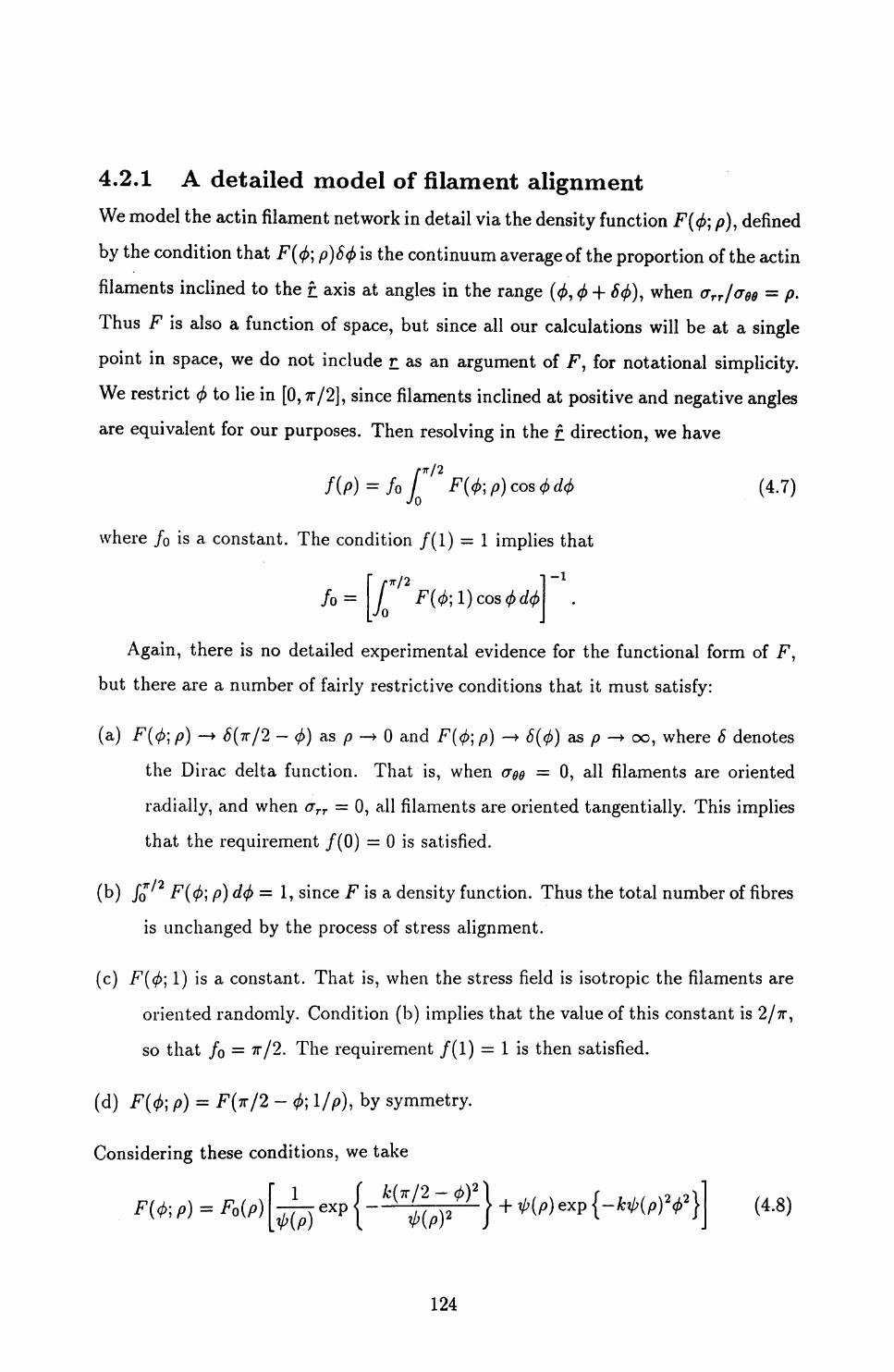
4.2.1 A detailed model of filament alignmentWe model the actin filament network in detail via the density function F(</>] /o), defined

by the condition that F((j>; p)8</> is the continuum average of the proportion of the actin

filaments inclined to the r axis at angles in the range (<£, <j> + 6<j>), when crrr /(7gg = p.

Thus F is also a function of space, but since all our calculations will be at a single

point in space, we do not include r as an argument of F, for notational simplicity.

We restrict 0 to lie in [0, ?r/2], since filaments inclined at positive and negative angles are equivalent for our purposes. Then resolving in the r direction, we have

= /o T Jo cos <W (4-7)

where /0 is a constant. The condition /(I) = 1 implies that

•7T/2

/o =,7

/Jo

Again, there is no detailed experimental evidence for the functional form of F, but there are a number of fairly restrictive conditions that it must satisfy:

(a) F($;p) — * 8(7r/2 — <£) as p — > 0 and F(<j>',p) — > 6(<t>) as p — > oo, where 8 denotes

the Dirac delta function. That is, when &ee — 0, all filaments are oriented

radially, and when crrr — 0, all filaments are oriented tangentially. This implies

that the requirement /(O) = 0 is satisfied.

(b) /o^2 F((j); p) d(j> = 1, since F is a density function. Thus the total number of fibres

is unchanged by the process of stress alignment.

(c) F($; 1) is a constant. That is, when the stress field is isotropic the filaments are

oriented randomly. Condition (b) implies that the value of this constant is 2/?r,

so that /0 = 7T/2. The requirement /(!) = ! is then satisfied.

(d) F(<f>; p) = F(7r/2 - <t>; !//>), by symmetry.

Considering these conditions, we take

/O — W^l , _ _/(4.8)1 exp<-

124

Figure 4.3: The form of F(<j>;p), defined in (4.8), plotted as a function of

p p =0.01, 0.05, 0.1, 0.2, 0.3, 0.5, 0.75, 1.0; F(Q-,p) increases with pf., for

where k is a positive constant and ^(0) = 0, ^(1) = 1 and ^(oo) = oo. F0(p) is

chosen such that condition (b) is satisfied. The form (4.8) satisfies condition (a),

since the Dirac delta function satisfies

8(x) = lim — 7= exp ( — x2 /e2 } v ' ^O \ ' '

= p p for(see, for example, Courant and Hilbert, 1962). Further, if we take

some p > 0 then condition (d) is satisfied.

It remains to consider condition (c), which is equivalent to the condition that

g(<t>) = exp \-ktf] + exp [-fc(jr/2 - <t>) 2} (4.9)

is constant on 0 < (j> < K/2. While this does not hold exactly for any non-zero value

of fc, it is approximately true for values of k close to 1. We choose k to minimize

the variation of g((j>) on [0,7r/2], and we show below that this gives k « 0.988. The

variation of g(<j>) on [0,7T/2] is then less than 3%.

F((j); p) is plotted in Figure 4.3 as a function of (j> for a range of values of p p in [0,1];

the parameter p remains undetermined. The form for f(p) implied by this function F

is shown in Figure 4.4, in which we plot both /(/?) and /(!//>) against p p for 0 < p < 1.

125

1.4

2,2J3

0.8

0.2

0.2 0.4 0.6 0.8 1.0

Figure 4.4: The functions f(p) (full curve) and h(p) (dashed curve) plotted against p p . Here h(p) — (1 -f- a)p p/(p p + a), and the form of f(p) is that defined in terms of F((j>\p) in (4.7), with F((j>;p) defined in (4.8). Rather than plotting on [0,oo), we plot both f(p) and /(1//9), and h(p) and /i(l//?), on [0,1]. The close approximation of h(p) to f(p) justifies the form given for f(p) in (4.5), and predicts the value of the constant a as (?r/2 — 1).

These functions were calculated by evaluating the integral in (4.7) numerically for a

range of values of p p . In Figure 4.4 we also plot h(p) = (l + a)p p/(p p + a) and h(l/p)

against /? p , with a chosen such that h(oo) = /(oo). Specifically, (4.7) and properties

(a) and (c) of F((j>\p] together imply that•7T/2

cos/•7T TT

/(oo) = / - Jo 2

so that a = ?r/2 — 1. This value of a is independent of p. Thus

h(p) = (ir/2)p p/(p p + 7T/2 - I) . (4.10)

It is clear from Figure 4.4 that to a good approximation, the form (4.8) for F(^ p)

implies thatf(p) = ( 7r /2 )()P . (4.11) J W pp + Tr/2-l V '

If we choose p = I for algebraic simplicity, this is the form given in (4.5), with

a = 7T/2 — 1. Until relevant experimental data is available, it is inappropriate to take

more complicated functional forms.

126

4.2.2 The value of kWe now determine the value of k, not near zero, that minimizes the variation oi

defined in equation (4.9), on 0 < </> < Tr/2. (Trivially, g(</>) = 2 when k = 0, but this

case is not biologically relevant). The form of g(<j>) for a selection of values of k is shown in Figure 4.5. Differentiating (4.9) with respect to <j> gives

dgexp {k7r((f> — 7T/4)} —

Therefore

(4.12)

It is sufficient to consider this equation on [0,?r/4], by the symmetry of g((/>) about

</> = 7T/4. The two sides of (4.12) are plotted in Figure 4.6 for a range of values of k. From this, it is clear that in addition to the root at ^ = 7T/4, equation (4.12) has a second root in (0,7r/4) if k > fccr ; tl , where kcr it \ satisfies

exp {k7r((j> — 7T/4)} —7T/2 -

= 0

This uniquely determines Arcria as 8/7T 2 , w 0.81.

We now write

9max(k) = max g(<j)) and gmin (k) = min

By symmetry these are also the maximum and minimum values respectively on

[0,7r/4]. Then for k < kcritl ,

and gmin (k) = g(0) = 1 +

For k > kcriti, (Jmax(k) = (j((j>max}, where ^max is the unique solution of

in the open interval (0,7r/4). This cannot be found analytically, but can easily

be calculated numerically for a given value of k. Also, for k > fccr,a,

127

1.501.45

1.401.351.301.251.201.15

1.501.451.401.35

1.251.201.15

a0.4 0.8

<P1.2 7T/2

0.4 0.8 1.2 7T/2

1.50 1.45- 1.40-

1.35-

1.2011.15

1.501.451.40

1.353 1.3000

1.251.20

1.15

0.4 0.8 1.2 n/2

0.4 0.8 1.2 tr/2

Figure 4.5: The form of the function #(0), defined in (4.9), as the parameter k varies, (a) k = 0.7; (b) k = 0.93; (c) k- = kcrit2 w 0.988 (see page 130); (d) k = 1.1. The dashed line indicates the equal values of </(0) and #(7r/2).

128

0.1 0.2 0.3 0.4 0.5 0.6 0.7 n/4

Figure 4.6: The right-hand (full curve) and left-hand (dashed curves) sides of equa­ tion (4.12) for k =0.2, 0.4, 0.6,.. .,2.0; the value of the left-hand side decreases, for any given </>, as k increases. The number of solutions of the equation on [0,7T/4] increases from one to two as k increases through a critical value, kcr it\.

min{<7(0),<y(7r/4)}. It is clear from Figure 4.5 that there is a critical value kcri t 2 such that

, so that gmin(k) = 1 +

, so that gmin(k) = 2e~

for kcrit i < k <

and for k > kcrif2\ #(0) > tf(7r

Here kcr i t 2 satisfies #(0) = g(7T/4), that is

4.

Thus kcriti. = -(16/7T2 ) logo;, where a: is a solution of x4 - 1x + 1 = 0. Now

x — = (x- l)(x' x - .

The root x = 1 corresponds to the trivial case of g(4>) = 2 when k = 0. The cubic

equation has the form

17 Q / 1 \where *y =

129

k=kcrtU

1.0k

1.5 2.0

Figure 4.7: The maximum and minimum values of g(<t>) on [0,;r/2], gmax(k) and gmin(k), plotted as functions of the parameter k. The vertical lines k = kcrit\ and k = kcrit2 are also drawn.

We now substitute 7 = sinh£, which gives a 1-1 correspondence between 7 and f. Using the identity

sinh 3f = 4 sii

this gives

so that the cubic equation has a unique solution, and

16 2V5 —— smh 1 . ! -smh 17 0.987886 .

In Figure 4.7 we plot gmax(k} and gmin (k) as functions of k. These suggest that the variation of g(</>) is minimized when k = kcrit2 , and this is confirmed by numerical minimization using quadratic interpolation. Specifically, numerical calculations show that both [gmax(k)-gmin(k)} and [gmaX (k)-gmin(k)]/[gmaX (k)+gmin(k)} are minimized at k = kcrit2, fork not near zero. (Trivially, gmax (k) = gmin(k) when k = 0, since then g(</>) = 2). Thus the variation of g(</>) on 0 < </> < n/2 is minimized in both an

absolute and relative sense when k =

130

4.3 Solutions of the Improved Model4.3.1 One-dimensional solutionsTo incorporate the concept of filament alignment into the one-dimensional model

equations, we consider a two-dimensional epithelial sheet in cartesian coordinates,

with no variation in the y-direction. The dimensionless stress tensor £, without inclusion of stress alignment of actin filaments, is then given by

0<7 = k "

0

where G = 1/(1 + ux] is the scalar actin filament density. The procedure for incor­

porating actin alignment in a general two-dimensional geometry was explained on

page 123; in this case it is particularly simple since at all points the principal axes

of £ are aligned with the coordinate axes. Thus the diagonal components of the

'improved' stress tensor satisfy

1= f(&xx/&yy) (E + !>, +

1 pu3i

Using the functional form for / in (4.5), this implies

1 . Eux

yy

= G

= G

(3ux I-a aEux

1+0M. I-a

Substituting these into the governing equation V • g, — XGu gives

d_ dx

E 1u

-u = 0.\+ux lU-a ) * ' H

The boundary condition at the wound edge (x = 0, say) is crxx = 0, that is

(-^— + r) ux + 1 * = 0 at x = Q- \l - a J 1 + (3uxthe boundary condition at x = oo remains u = 0. This system, which is in fact

independent of the form of <7yy , differs from (3.5) subject to (3.6) only in E being

replaced by E/(l — a). Therefore, the analytical and numerical investigation in

Section 3.3 remains valid if we reinterpret E as E/(l - a) + T.

131

4.3.2 Two-dimensional radially symmetric solutionsThe relations (4.1) and (4.6) together imply that in a radially symmetric geometry, the

non-zero components of the dimensionless stress tensor incorporating stress alignment of actin filaments are

<JT- =_ E(u' — au/r]

E(u/r -

)/(! - a) + r(u' + u/r) + 1/[1 + P(u' + u/r + uu'/r)} 1 -f u' -f u/r + uu'/r

- a) + F(u' + u/r) P(u' + u/r + uu'/r)}.(4.13b) 1 -f- u' + u/r + uu'/r

Substituting these into the governing equation V • £ = \Gu and using the expression

for the divergence of a tensor in plane polar coordinates given in (3.13) gives

d• ^^^

dr' -fra (u' - au/r) + T (u' + u/r) + 1/[1 + /?(u' + u/r -f uu'/r)]

W + u/r -f uu'/r

u' — w/r \ru(4.14)Vl — a/ \l +u' + u/r + uu'/r J 1 + u' + u/r + uu'/r '

Note that the substratum adhesion term is proportional to the scalar actin filament

density, and is unaffected by stress alignment of the actin filaments. Expanding (4.14)

gves

( . u uu 1 + u' + - -f — r r

£ (u»_- + ^|_rr r-1

uu" u'2 uu'+ ___

I.. u u uu u" + — - — + —

" u'2 uu'~r — — —r~

ruu r

1 + /? + 2^(u' + u/r + uu'/r) [1 + fi(u' -f u/r + uu'/r)] 2

«) ( w/ ~ -) V r)

.1 + u' + - ru uu .

= Aru 1u- r

uu r

where £ = E/(l - a). Writing

~1 + (3 + 2/?(u7 + u/r + uu7/r)

' + u/r + uu'/r)] 2 '

this simplifies to

u — — . r,

Aru

uu

. u uu 1 + u' + - + —— r r

. (4.15)

132

The boundary conditions are arr — 0 at r = 1, the wound edge, and u — 0 at r — oo.

Using (4.13a) and simplifying, the boundary conditions become

u' - au) + T(u' + u) +—_——__ = Q at r = 1 (4.16a)1 -f p(u' + u/r + uu' IT)

u = 0 at r = oo. (4.16b)

We solved (4.15) subject to (4.16) numerically, using continuation in ft. That

is, we gradually increased 0, using the solution for the previous ft as the initial ap­

proximation at each stage. The solution for ft — 0 was obtained using the solution

for ft = a = 0 as the initial approximation; numerical determination of this latter

solution was discussed in Section 4.1. As in both the one-dimensional solutions inves­

tigated in Sections 3.3 and 4.3.1, and the two-dimensional solutions without filament

alignment, presented in Section 4.1, there appeared to be a critical upper limit on the

value of ft, above which solutions could not be obtained. Moreover, as ft approached

this critical upper limit, flcrit say, the band of aggregated actin at the wound edge

became sharper, so that the model solutions did reflect the phenomenon of the actin

cable. However, in contrast to solutions in the absence of filament alignment, we

were able to capture both this phenomenon and the more superficial aspects of the

response to wounding observed experimentally, that is a retraction of the wound

edges by 10-15%, with only the leading 4-5 cell layers significantly contracted. Such

a solution is illustrated in Figure 4.8. In previous illustrations of model solutions,

we have plotted the scalar actin filament density G(r). However, for this improved

model, more relevant functions are the effective dimensionless densities of filamen­

tous actin aligned radially and tangentially. These are Gr (r) = f(crrr/<T60) • G(r) and

Gg(r) = f(o-00/<rrr ) • G(r) respectively. Using (4.13), these are

+ u/r) + 1/[1 + (3(u' + u/r + uu'/r)] + E(u' - au/r) r ~ (n ' + u/r) + 1/[1 + ft(u' + u/r + uu'/r)} + (1 - a)Eu' ( }

u/r) + !/[!+ P(u' + u/r + uu'/r)} + E(u/r - au')

where G(r) = 1/(1 + u1 + u/r + uu'/r). The parameter values A, E, F and a used

in Figure 4.8 are consistent with the biologically relevant one-dimensional solutions

discussed in Section 3.3, since we are interpreting E = E + F. However, the value of

133

0.12 i

0.10

0.08^—^

^0.06

0.04

0.02

a

1.02 1.04 1.06 1.08 1.10r

1.02 1.04 1.06 1.08 1.10r

1.02 1.04 1.06 1.08 1.10r

Figure 4.8: (a) The numerical solution of (4.15) subject to (4.16). (b,c) The cor­ responding effective radially and tangentially aligned dimensionless actin filament densities G> and GO, defined in (4.17). The parameter values are A = 3.0, E = 0.3, P = 0.8, (3 = 0.31, a = 7T/2 — 1; this value of the filament alignment parameter a is that predicted by the heuristic model of the actin filament network (see Section 4.2). This solution captures the key aspects of the experimentally observed response of the epidermis to wounding.

134

is significantly smaller than in the one-dimensional geometry, as explained in the next section.

4.4 The Critical Upper Limit on ftNumerical solutions of the model suggest that for given values of A, E, F and a, the

value of the critical upper limit ftcrit on the value of the parameter ft is different in the one-dimensional and two-dimensional radially symmetric geometries. While we have been unable to derive an exact analytical expression for /3cr it in the latter case, we have obtained an analytic approximation that is valid for large A. As explained

in Section 4.5, biologically relevant solutions certainly require A > 1.

Recall that the nondimensionalization we have used implies that the dimensionless parameter A = A/?2 , where R is the dimensional wound radius, and the dimensional

quantity A is the ratio of the dimensional parameters Adim and TQ. But in the limit R —» oo, the radially symmetric geometry approaches the one-dimensional geometry, in which the critical upper limit on ft is [1 — l/(E + F)] (see Section 3.3). Thus as A —» oo, (3cr it — 1 — l/(E + F) + o(l). Here A denotes the dimensionless parameter.

The one-dimensional equations were analysed fully in Section 3.3, and we showedthere that as ft —* 1 — l/(E + F), ux w. e —> —1. Here 'l^.e.' denotes 'at the wound edge'. Recalling (3.7), that |Au2 = P(ux ) in °ne dimension, the displacement at the

wound edge in this limiting case is given by

u

'2 2- ftA ' ft(l-ft)

2 A

1/2

1/2

Now in one dimension, A = AL2 , where L is the length scale used in the nondimen- sionalization. Thus the dimensional value of the displacement at the wound edge in

135

the one-dimensional geometry is

ti(0).L r) - r)1/2

(4.18)

Returning to the two-dimensional radially symmetric geometry, the singularity

as /3 —>• Peru arises in this case because du/dr(l) —> — 1. Therefore the boundary

condition (4.16a) implies that in this critical case

1 i«(!) =

Now in the limit as the wound radius R —> oo, the dimensional displacement at the

wound edge in the two-dimensional radially symmetric geometry must tend to the

dimensional displacement at the wound edge in the one-dimensional geometry. (Of

course, the dimensionless displacement tends to zero). That is, as R —> oo,

R ( =. - 1F -aE 1-0crit

2^ A

- 2(E + F)1/2

iT-aE

2 A

as A —> oo. Simplifying this gives

r) - r)1/2

+ o (A' 1 / 2)

r - (r - (4.19)

as A —> ex), where

2 A

This approximation is illustrated in Figure 4.9, where for given values of E, F and

a we have estimated ftcrit numerically for a number of values of A. These numerical

estimates are obtained by successively increasing /? in the continuation numerical

method, with smaller and smaller increments, until u'(l) < -0.999995.

136

0.33-

0.32

0.31

0.30-

Num. estimate Anal, approx.

4 5 678 10 A

20 30 4050

Figure 4.9: The analytical approximation (4.19) of /?crtt compared to numerical esti­ mates for a range of values of A. The other parameter values are E = 0.3, F = 0.8, </ = 7T/2 — 1. For clarity, A is plotted on a logarithmic scale.

An important issue raised by the model is the biological interpretation of the result

that solutions only reflect the phenomenon of the actin cable when (3 is very close

to j3Crit- Such an interpretation emerged when we examined the biological literature

on the relative rates of intracellular rearrangement of myosin and filamentous actin.

Myosin is a generic term for a class of proteins that bind to filamentous actin. While

the role of myosin in muscle contraction has been understood for some time (see, for

example, Alberts et al., 1989, Chapter 11), many questions concerning nonmuscle

myosins remain unanswered; for a detailed review, see Korn and Hammer (1990).

However, there is little doubt that the exertion of traction forces by actin filaments

does depend on interaction with myosin (Citi and Kendrick-Jones, 1987; Langanger

et a/., 1986).

In experiments described above on actin filament reorganization, Chen (1981) and

Kolega (1986) found that this process occurred on the time scale of a few seconds. In

contrast, Nachmias et al (1989) investigated the intracellular movement of myosin in

Dictyostelium discoideum amoebae following a micromolar stimulus of cyclic AMP,

and found that myosin translocation to the cell cortex was considerably slower, with

137

a maximal response after about 2 minutes. McKenna et al. (1989) observed the

movement of "bead-like" myosin-containing structures in 3T3 fibroblasts following

microinjection with fluorescently labelled myosin. They observed a movement to­

wards the centre of the cell with a speed of 0.18 (± 0.09) /zm/min, which would

again correspond to a time scale of a few minutes for post-wounding myosin reor­

ganization. Finally, DeBiasio et al (1988) studied the actin and myosin content of

cellular protrusions in migrating Swiss 3T3 fibroblasts by microinjecting fluorescent

derivatives. They found that while actin was present in these protrusions initially, in

fact at somewhat elevated levels, myosin only became detectable after 1-2 minutes.

Thus it seems that the reorganization of actin filaments in response to wound­

ing might be considerably quicker than the corresponding movement of intracellular

myosin. Recalling that the parameter 0 reflects the extent of myosin cross-bridging

between actin filaments, we can think of ft as a parameter whose value increases grad­

ually with time. With this interpretation, we can regard the variation in the model

solutions with increasing /3 as the time evolution of epidermal displacements in the

first few minutes after wounding. The corresponding sequence of scalar actin filament

densities G(r\ ft] is illustrated in Figure 4.10. In this figure, G(r; 0) is plotted against

u -f r, the post-wounding radial position of the material point initially at radius r.

This shows that as myosin rearrangement proceeds, not only does the actin aggrega­

tion at the wound edge increase, but also the wound edges begin to move inwards.

The parameter (3 is of course prevented from reaching (3crn by physical constraints

on the packing of actin filaments, which are not included in our model. We should,

however, stress that this interpretation of the variation of (3 is at best heuristic; full

theoretical investigation of the role of myosin in the formation of the actin cable

would require new detailed modelling of actomyosin interaction in non-muscle cells.

138

frftr

-D*05-

4-3-^

1/9=0.0000

i^

9- 8-7-

^•6-o's-

4-3-2-

1.2 1.4 ' Teu(r)+r

1 flgQ.0800

17=0-2876

1.2 1.4 u(r)+r

1.2 1.4 1.6 u(r)+r

1.2 1.4 1.6 u(r)+r

Figure 4.10: The scalar actin filament density G(r) plotted against u(r) + r, for a range of values of the parameter /?. The other parameter values are A = 1.5, E = 0.29, P = 0.77, a = 7T/2 — 1. For these values, we estimate numerically that /?crt-t w 0.28784. When (7(1.0) is greater than the upper limit of the vertical axis, its value is indicated. Since we are interpreting /3 as a parameter whose value increases gradually with time, we can regard this figure as a time sequence of actin filament densities during the first few minutes after wounding.

139

4.5 Appropriate Parameter ValuesWe have shown that in the limit as ft —* ftcrit , the solutions of the improved model

(4.15) subject to (4.16) can reflect the experimentally observed response of embryonic

epidermis to wounding. One aspect of this response involves conditions on the post-

wounding displacements. In this section, we investigate the effects of variations in the

parameters A, E , F and a on the limiting value of these displacements u(r) as ft —>

(3crit. In the absence of a full analytic solution, these limiting displacements can only

be estimated numerically. Our method of numerical solution involves gradual increase

in the parameter /?, with successively smaller increments, using the solution for the

previous value of (3 at each stage (see page 133). Therefore, numerical estimation

of the limiting displacements requires a stopping criterion: when this criterion is

satisfied, we can end our incrementation of ft and take the current u(r) as a good

approximation to the limiting displacements. Such a criterion cannot involve the

value of either (3crn or lim/?-^., u(l), since we do not have analytical expressions

for these. However, as ft —> (3cr i t , w'(l) —» — 1, and we use this as the basis for our

stopping criterion. Table 4.1 shows numerically calculated values of u(l) and the

corresponding values of u'(l) as ft is increased, for a typical set of values of A, E, T

and a; the computer processing time required to achieve the last value shown was

about 26 hours on a 6 MIPS machine. These values suggest that u(l) is within 1%

of its limiting value when w'(l) = —0.99995. Based on this, we take the condition

tt'(l) < —0.99995 as our stopping criterion for the numerical increase of ft.

Having established this stopping criterion, we can investigate the effect of param­

eter variations. Figures 4.11 and 4.12 show the effect on u(r) and u'(r) respectively

of ±10% changes in the values of each of the parameters A, E, F and a, for a given

set of reference parameter values. To use graphs such as these effectively, we must

establish exact criteria under which the model solutions will be said to agree with

experimental observations. Since the experimental data is only semi-quantitative,

such criteria are necessarily somewhat arbitrary. However, they do make a precise

investigation of parameter variation possible, leading ultimately to the determination

of a full parameter domain. The qualitative form of this domain will not depend on

140

Effect of variations in a

0.12-

o.io-0.08-

0.06-

0.04-

0.02

Effect of variations in E

10.0% Incr. in aRet. params

10.0% deer, in a1.04 1.08

0.12-

0.10-

0.08-

0.06-

0.04-

0.02-10.0% incr in E

Ref parsons 10.0% deer in E

1.04 1.08

Effect of variations in F Effect of variations in A0.12-

0.10-

0.08-

^0.06-

0.04-

0.02-10.0% in^r in

Ref. paramo10.0% deer in

0.12-

0.10-

0.08-

^0.06-

0.04-

0.02-10.0% inc_r in A

Ret paramo 10.0% deer in A

1.04 1.08 1.04 1.08

Figure 4.11: The effect of parameter variation on the limiting solution lim/3_^cr . t u(r) of the improved model (4.15) subject to (4.16). The solutions in green are for the parameter values A = 3.0, E = 0.3, F = 0.8, a = ir/2 — 1. Those in red correspond to a 10% increase in one parameter, and those in blue correspond to a 10% decrease in that parameter. The r interval shown corresponds to the leading 5 cell layers. In contrast to Figure 3.6, these solutions are not highly sensitive to changes in any of the parameter values, because we are plotting the solution in the limit as /? - in this case, rather than fixing the value of ft.

141

Effect of variations in a

10.0% incr. in aRef. params

10.0% deer, in a

Effect of variations in E

1.04 1.08

10.0% incr in ERef. params

10.0% deer In E1.04 1.08

Effect of variations in F Effect of variations in X

10.0% incr in rRef. params

10.0% deer in r

10.0% incr in XRef. params

10.0% deer in X

1.04 1.08 1.04 1.08

Figure 4.12: The effect of parameter variation on the first derivative Iim0_>/3cr, t u'(r) of the limiting solution of the improved model (4.15) subject to (4.16). The solutions in green are for the parameter values A = 3.0, E = 0.3, F = 0.8, a = ir/2 — 1. Those in red correspond to a 10% increase in one parameter, and those in blue correspond to a 10% decrease in that parameter. The r interval shown corresponds to the leading 5 cell layers. In contrast to Figure 3.7, these solutions are not highly sensitive to changes in any of the parameter values, because we are plotting the solution in the limit as -* ftr* in this case, rather than fixing the value of /?.

142

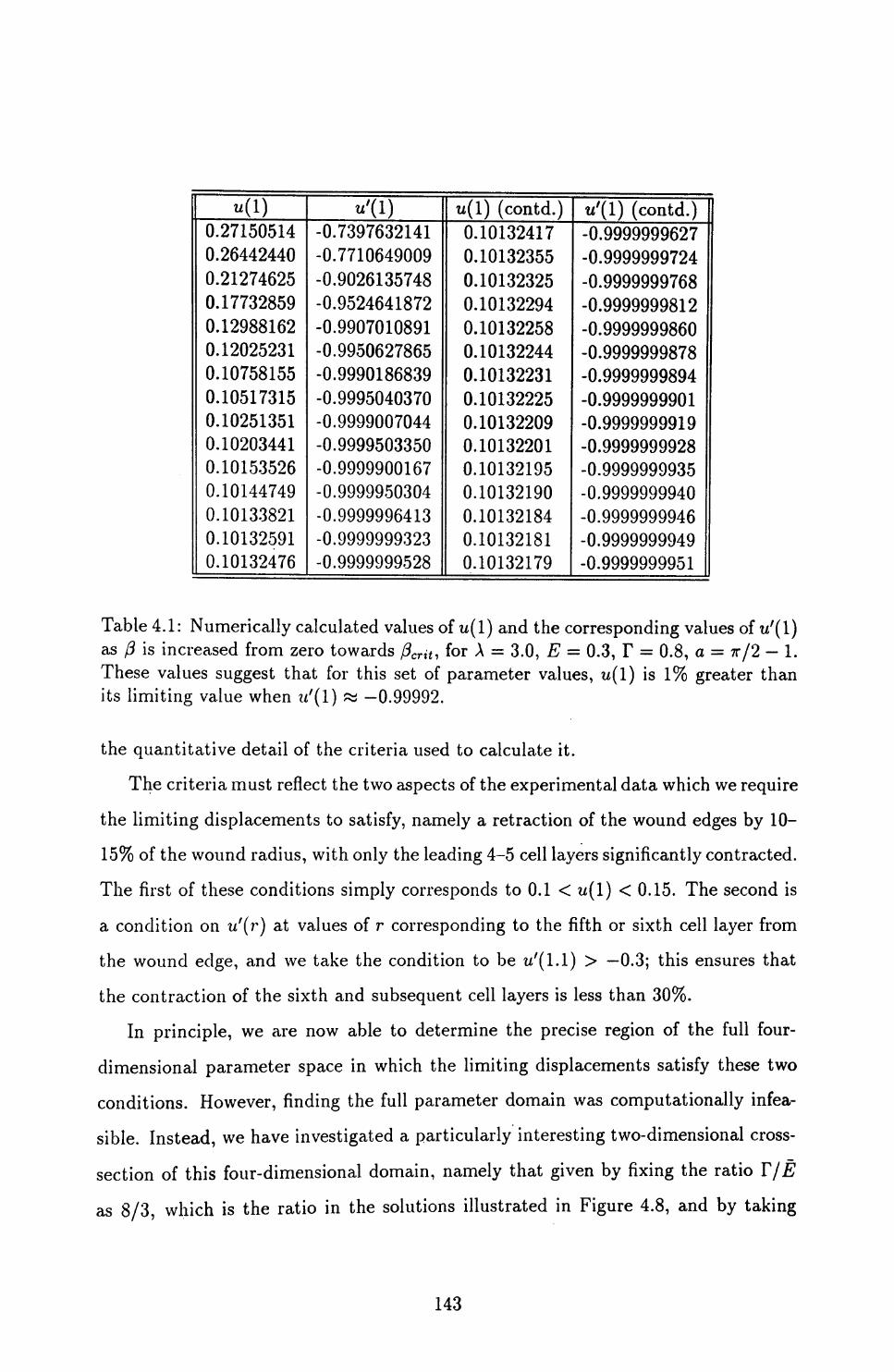
f(l)0.271505140.264424400.212746250.177328590.129881620.120252310.107581550.105173150.102513510.102034410.101535260.101447490.101338210.101325910.10132476

"'(1)-0.7397632141-0.7710649009-0.9026135748-0.9524641872-0.9907010891-0.9950627865-0.9990186839-0.9995040370-0.9999007044-0.9999503350-0.9999900167-0.9999950304-0.9999996413-0.9999999323-0.9999999528

u(l) (contd.)0.101324170.101323550.101323250.101322940.101322580.101322440.101322310.101322250.101322090.101322010.101321950.101321900.101321840.101321810.10132179

w'(l) (contd.)-0.9999999627-0.9999999724-0.9999999768-0.9999999812-0.9999999860-0.9999999878-0.9999999894-0.9999999901-0.9999999919-0.9999999928-0.9999999935-0.9999999940-0.9999999946-0.9999999949-0.9999999951

Table 4.1: Numerically calculated values of u(l) and the corresponding values of u'(l) as (3 is increased from zero towards /?crt<, for A = 3.0, E = 0.3, F = 0.8, a = Tr/2 — 1. These values suggest that for this set of parameter values, w(l) is 1% greater than its limiting value when u'(l) w -0.99992.

the quantitative detail of the criteria used to calculate it.The criteria must reflect the two aspects of the experimental data which we require

the limiting displacements to satisfy, namely a retraction of the wound edges by ID- 15% of the wound radius, with only the leading 4-5 cell layers significantly contracted. The first of these conditions simply corresponds to 0.1 < u(l) < 0.15. The second is a condition on u'(r) at values of r corresponding to the fifth or sixth cell layer from the wound edge, and we take the condition to be w'(l.l) > -0.3; this ensures that the contraction of the sixth and subsequent cell layers is less than 30%.

In principle, we are now able to determine the precise region of the full four- dimensional parameter space in which the limiting displacements satisfy these two conditions. However, finding the full parameter domain was computationally infea- sible. Instead, we have investigated a particularly interesting two-dimensional cross-

section of this four-dimensional domain, namely that given by fixing the ratio T/E as 8/3, which is the ratio in the solutions illustrated in Figure 4.8, and by taking

143

a = 7T/2 — 1. This value of a is that predicted by the detailed heuristic model of the

actin filament network developed in Section 4.2. This cross-section is of particular in­

terest because of its relevance to the one-dimensional system, in which the ratio T/E

is irrelevant, and only the sum (E + F) is important. The form of the cross-section is

shown in Figure 4.13. In this figure, we have taken ten equally spaced values of A and

ten equally spaced values of (E + F), and for each of the 100 parameter sets we have

determined whether or not the limiting displacements satisfy the above conditions.

The figure also shows contours of the value of 0 reached when the stopping criterion

was satisfied; this is a numerical estimate of the critical upper limit

4.6 ConclusionsThe recent discovery by Martin and Lewis (1991a,b) of an actin cable at the wound

edge in embryonic epidermal wounds raises a number of interesting and important

biological questions, prominent amongst which is the issue of how the cable forms

over such a short time scale. In this chapter we have addressed the possibility that the

cable forms by compaction and reorientation of the actin filament network, without

either depolymerization of actin in one part of the cell and corresponding repolymer-

ization in another part, or intracellular movement of intact actin filaments, or de novo

synthesis of filamentous actin. Although there is experimental evidence that this is

the mechanism of cytoskeletal reorganization in some in vitro situations (Chen, 1981;

Albrecht-Buehler, 1987), this is very much a hypothesis.

Our modelling has investigated the new equilibrium state of the actin filament

network after wounding, under this hypothesis. We have shown that this mechanism

can explain the actin cable observed experimentally, and that if this is the mechanism

of formation, it depends crucially on the properties of actin filament alignment in re­

sponse to stress and of actin filament synergy in cell traction forces. The latter prop­

erty involves interaction between intracellular actin and myosin, and we have been

able to interpret the singular limit near which the model captures the phenomenon

of the actin cable in terms of the relative rates of post-wounding rearrangement of

144

1.12-

1.11-

+ 1.09

1.08-

1.07-

1.06-

1.50 1.75 3.QO 2.$5 2.50 2.75 3.QQ 3.^5 3.$0

'0.320-

•o.a to-

•0.305-—

•0.300—

Criteria satisfied Criteria not satisfied

Figure 4.13: A two-dimensional cross-section of the full four-dimensional parameter space, given by fixing a = 7T/2—1 and T/E = 8/3. For each of the 100 parameter sets, the conditions 0.1 < w(l) < 0.15 and ti'(l.l) > —0.3 were tested on the numerical estimates of the limiting displacements. The points are marked with red circles or blue squares, corresponding to these conditions being satisfied or not satisfied, respectively. Contours of the corresponding numerical estimates of (3^^ are shown in green.

145

act in and myosin.

To clarify the agreement between the model solutions and experimental data, we

have used these solutions to simulate an optical section through the basal layer of

the epidermis, after staining with fluorescently tagged phalloidin. We described on

page 72 how Martin and Lewis (1991a,b) used this staining technique to visualize

the actin cable experimentally; a typical experimental result is shown in Figure 3.2.

To simulate this experimental photograph from our model solutions, we treated the

filamentous actin distribution predicted by the model, appropriately normalized, as a

probability distribution for phalloidin staining. Thus we marked in white, against a

black background, the post-wounding positions [w(r)+r]r of a large number of points,

with radial coordinate chosen at random from this distribution, and angular coordi­

nate chosen at random from a uniform distribution. We found that about 9 million

points were required to give a 'staining level' equivalent to that used experimentally.

Such a simulation is shown in Figure 4.14; it compares well with the corresponding

experimental result (Figure 3.2).

We end this chapter by suggesting three possible experimental approaches to

testing the basic conclusion of our modelling, that the formation of an actin cable in

response to wounding in embryonic epidermis is consistent with the assumption that

the amount of filamentous actin in a given region of cytogel remains constant as that

region is deformed. The first involves detailed quantitative experiments to determine

whether the parameter values for which the model predicts the formation of the actin

cable are appropriate for the cell types in which the cable has been observed. The

relevant quantitative data currently available is reviewed on page 79.

The second experimental approach is to investigate the wounding response in the

presence of cytochalasin. This is the generic name for a group of fungal metabolites

which act as actin filament capping proteins; cytochalasins B and D are the most

commonly used. Their function has been reviewed by Cooper (1987). Briefly, they

bind to the barbed ends of actin filaments, in a ratio of about one molecule per

filament and inhibit both association and dissociation of actin filament subunits

at that end. (The structure of actin filaments, including their inherent polarity, is

146

Exposed Actin Retracted mesenchyme cable epidermis

Figure 4.14: A simulation of an optical section through the basal layer of the epider­ mis after staining with fluorescently labelled phalloidin, as predicted by the model solutions. We treat the filamentous actin distribution predicted by the model, appro­ priately normalized, as a probability distribution for phalloidin staining. The figure shows the post-wounding positions of 9 million points, with radial coordinate chosen at random from this distribution, and angular coordinate chosen at random from a uniform distribution. The parameter values are A = 1.5, E = 0.29, F = 0.77, a = 7T/2 -!,/? = 0.2876. For these values of A, E, T and a, /3crit « 0.2878. (Scale bar =

discussed in the book by Alberts et a/., 1989, Chapter 11, and in more detail in the

recent review by Pollard, 1990). For example, Bonder and Mooseker (1986) found

a reduction of about 90% in both the association and dissociation rates of subunits

at the barbed ends of acrosomal actin filament bundles in Limulus sperm, at the

(relatively high) concentration of 2/iM of cytochalasin B.

In an in vivo study on HEp-2 cells, Morris and Tannenbaum (1980) successfully

used cytochalasin to stabilize the filamentous actin concentration, and we suggest

that it might be possible to use cytochalasins in a similar way in the embryonic

wounding system. If this were possible, our hypothesis would predict that many

147

aspects of the initial response to wounding, including the formation of the actin cable,

would be unaffected. However, some studies have found cytochalasins to have highly

disruptive effects on the actin filament network. For example, Schliwa (1982) found

that cytochalasin D caused extensive disruption to the cytoskeleton of African Green

Monkey kidney cells, over a time scale of a few minutes, and Forscher and Smith

(1988) found that cytochalasin B caused almost complete loss of filamentous actin

in growth cones from Aplysia neurons, again within a few minutes. Further, Pollard

(1990) urges caution when interpreting experiments involving cytochalasins because

of difficulties arising from the low-affinity binding of cytochalasins to actin monomers.

Thus, a necessary precursor to any investigation of the response to wounding in the

presence of cytochalasins is a preliminary study to determine the precise effects of

the various cytochalasins on the embryonic epidermal cells concerned, in a control

situation.

The final possible experimental approach to testing our hypothesis involves the

technique of photobleaching, which has been used by Wang (1985, 1987) to study

the actin filament network. The technique is to first microinject cells with fluores-

cently labelled actin, a procedure which is now well established (Pollard, 1990). The

fluorescent actin is rapidly incorporated into the filament network, which in most

systems then functions normally. Wang's approach is to then photobleach a spot

of the fluorescent filament network, a few //m across, and to follow the subsequent

progress of the bleached region. In the 1985 study, Wang used this technique to in­

vestigate the movement of actin subunits within lamellipodia of gerbil fibroma cells,

and in the 1987 study he used it to investigate the reorganization of actin filaments

during division of 3T3 cells. We suggest that it might be possible to amend this

technique to study in detail the dynamics of the actin filament network after wound­

ing. Again, preliminary investigations in control situations would be necessary to

determine whether or not this is a viable experimental approach. In particular, it

requires that the rate of movement of actin subunits within filaments is not too large

in the cell type concerned.

In conclusion our modelling predicts that the formation of the actin cable ob-

148

served by Martin and Lewis (1991a,b) is consistent with the hypothesis that the

amount of filamentous actin in a given region of cytogel remains constant as that

region is deformed. Moreover, we have suggested three approaches to testing this

model prediction experimentally.

149

Chapter 5

Chemical Control of CellMovement and the Boyden

Chamber Assay

5.1 Biological Background and Previous ModelsIn the Introduction, we discussed the important role played in dermal wound healing

by chemical regulation of cell motion, via both chemotaxis and chemokinesis. In

this chapter we develop a new model for chemically controlled cell movement. We

focus on endothelial cells, which move into the wound space in response to chemical

stimuli during the process of angiogenesis, resulting in a dense capillary network in the

granulation tissue of healing dermal wounds. However, the model is also applicable

to other aspects of wound healing, in particular the influx of white blood cells during

the early "inflammation" phase of healing, and the invasion of the wound space by

fibroblasts during the formation of granulation tissue.

To clarify a serious confusion of terminology, Keller et al. (1977) proposed def­

initions of the terms chemotaxis and chemokinesis which established their current

meanings. They defined chemokinesis as "a reaction by which the speed or frequency

of locomotion and/or the frequency and magnitude of turning of cells or organisms

moving at random is determined by substances in the environment", while chemotaxis

is "a reaction by which the direction of locomotion of cells or organisms is determined

by substances in their environment". Although there is still debate in the biological

literature on some finer points of the interpretation of these definitions (Wilkinson,

1988a,b; Bignold, 1988a), the terms are now in widespread use.

The available experimental evidence, reviewed by Devreotes and Zigmond (1988),

suggests that chemotaxis and chemokinesis occur in eukaryotic cells via the binding

150

of regulatory chemicals to receptors on the cell surface; the number and location

of bound receptors modulates pseudopod extension and thus cell motion. The sys­

tems that have been studied in most detail are the response of polymorphonuclear

leukocytes to N-formylated peptides and of Dictyostelium discoideum amoebae to

cyclic AMP. The mechanisms in the two cases are remarkably similar. The receptor-

chemical complex is rapidly internalized in intracellular vesicles, and once inside the

cell it dissociates, yielding free intracellular chemical and receptors. Experiments and

modelling by Zigmond et al. (1982) suggest that in at least the leukocyte-peptide

system, the intracellular chemical is partitioned into two pools, with a proportion

of the chemical degraded and released, and the remainder kept in a long term 'stor­

age pool'. The internalized receptors appear to be recycled back to the cell surface

(Sullivan and Zigmond, 1980; Van Haarstert, 1987), and moreover in the presence of

extracellular regulatory chemical, additional receptors (up to 30-fold) can be released

to the cell surface from an intracellular pool (Janssens and Van Driel, 1984; Zimmerli

et a/., 1986; Fletcher and Gallin, 1980).

A number of mathematical models have been proposed for chemically modulated

cell movement. The oldest and most widely used is the continuum model of Keller

and Segel (1971a,b). They take the cell flux Jn to be directly dependent on the local

extracellular chemical concentration, via the expression

Jn = -Dn (c)Vn + XnW^Vc , (5.1)

Chemokinesis Chemotaxis andchemokinesis

where n and c are the local cell density and chemical concentration respectively,

and the transport coefficients Dn (c) and xn ( c) are strictly positive for all c. Since

variations in c affect both the magnitude and direction of the second term, this

term represents a combination of chemotaxis and chemokinesis effects, under the

definitions of Keller et al. (1977). This model was originally applied by Keller

and Segel (1971a,b) to bacterial movement, but has more recently been used with

considerable success in a wide range of cellular and whole organism applications. The

Keller-Segel approach takes no account of the role of receptor kinetics in the cellular

response to chemotactic and chemokinetic factors: indeed, these kinetics were very

151

poorly understood when the model was formulated. More recently, Segel (1976)

incorporated receptor kinetics into the model when applied to bacterial movement.

His model consists of 9 coupled partial differential equations, and a simplification

reducing the system to 6 equations is considered in a second paper (Segel, 1977b).

Subsequent experimental work on receptor modification in bacteria is reflected in the

models of Goldbeter and Koshland (1984) and Segel et al. (1986). However, this work

has little relevance to wound healing, since the receptor-based mechanisms responsible

for chemotaxis are quite different in bacteria and eukaryotic cells. In particular, the

latter respond to spatial gradients in the chemoat tract ant, while bacteria can only

modify the length of time they spend moving in a particular direction, in response

to a temporal gradient of chemical concentration.

At the single cell level, Tranquillo and coworkers have developed a detailed stoch­

astic model for the motion of a single leukocyte in the presence of chemoattractants

(Tranquillo and Lauffenburger, 1987; Tranquillo et al, 1988; Tranquillo, 1990). This

model applies exclusively to a single cell, but in an attempt to combine single cell and

cell population models, Rivero et al. (1989) proposed a continuum model in which

the transport coefficients are related to the parameters of a simple stochastic model

for the movement of an individual cell. Their expressions for these parameters in

terms of the number of bound receptors per cell and the extracellular concentration

of chemoattractant assume that the receptor-chemical binding is at equilibrium. Yet

another approach is used by Fisher and Lauffenburger (1987) and Charnick and

Lauffenburger (1990), who take cell-cell encounters to be determined by a random

walk that is biased due to chemotaxis.

5.2 Shortcomings of the Keller-Segel Approach, Highlighted by the Boyden Chamber Assay

The Boyden chamber assay is a relatively simple in vitro system which enables chemo-

tactic and chemokinetic effects to be quantitatively tested. The assay was developed

by Boyden (1962), and its subsequent use is reviewed by Bignold (1988b). It consists

152

x mcr. A

x=0

Upper well

Lower well

i ri k

Figure 5.1: A diagrammatic representation of the Boyden chamber assay.

of two wells separated by a thin filter whose porosity enables cells to crawl actively

through, but prevents passive falling of cells under gravity between the upper and

lower wells (Figure 5.1). The lower well is filled with a solution of the chemical under

test, and the filter is placed on top of this. The pores of the filter rapidly fill with

the chemical solution, due to capillary action. The upper well is then filled with a

suspension of the cells under test; the cells rapidly settle onto the top of the filter.

The system is left for a given length of time (a few hours), during which the cells

crawl through the filter in response to the concentration gradient in the regulatory

chemical. Having passed through the filter, the cells rapidly spread across the lower

surface of the filter; they are prevented from dropping into the lower well by coating

the filter with an adhesive substance such as fibronectin. At the end of the given time

period, the number of cells on the lower surface of the filter is counted. To distinguish

between chemotaxis and chemokinesis, it is usual to repeat the experiment with the

cells in the upper well suspended in a solution of the chemical under test. A chemical

gradient will then only arise due to cellular degradation of active chemical.

In this section we apply a model based on that of Keller and Segel (1971a,b)

to chemically controlled cell movement in the Boyden chamber assay. Previously,

Lauffenburger and Zigmond (1981) and Lauifenburger et al (1988) have solved the

153

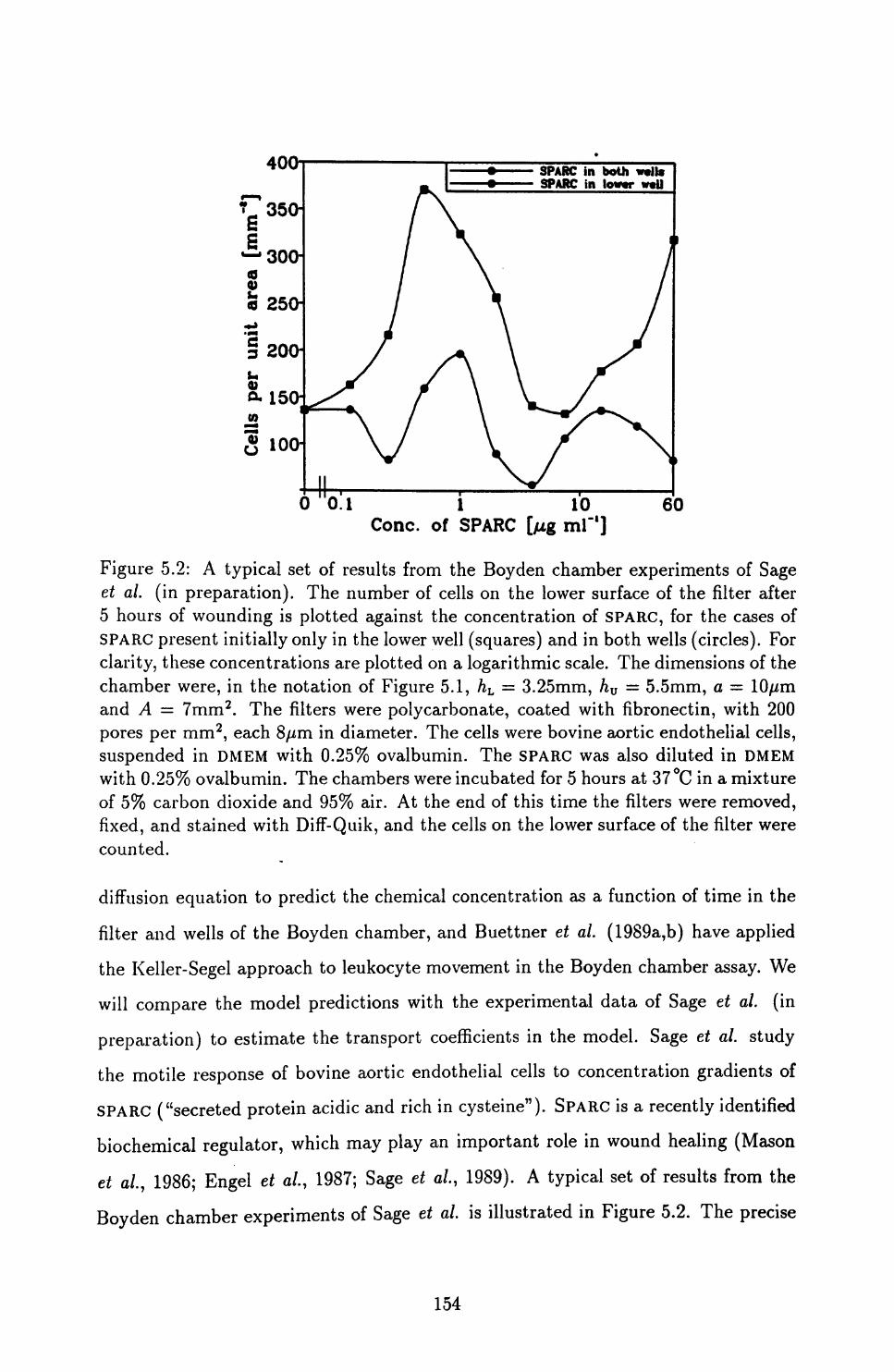
400 SPARC in both **»• SPARC in lovw well

0 0.1 1 10 Cone, of SPARC [fj.g ml" 1 ]

Figure 5.2: A typical set of results from the Boyden chamber experiments of Sage et ai (in preparation). The number of cells on the lower surface of the filter after 5 hours of wounding is plotted against the concentration of SPARC, for the cases of SPARC present initially only in the lower well (squares) and in both wells (circles). For clarity, these concentrations are plotted on a logarithmic scale. The dimensions of the chamber were, in the notation of Figure 5.1, hL = 3.25mm, hv = 5.5mm, a — 10/mi and A = 7mm2 . The filters were polycarbonate, coated with fibronectin, with 200 pores per mm2 , each 8/zm in diameter. The cells were bovine aortic endothelial cells, suspended in DMEM with 0.25% ovalbumin. The SPARC was also diluted in DMEM with 0.25% ovalbumin. The chambers were incubated for 5 hours at 37 °C in a mixture of 5% carbon dioxide and 95% air. At the end of this time the filters were removed, fixed, and stained with DifF-Quik, and the cells on the lower surface of the filter were counted.

diffusion equation to predict the chemical concentration as a function of time in the

filter and wells of the Boyden chamber, and Buettner et al (1989a,b) have applied the Keller-Segel approach to leukocyte movement in the Boyden chamber assay. We will compare the model predictions with the experimental data of Sage et al. (in preparation) to estimate the transport coefficients in the model. Sage et al. study the motile response of bovine aortic endothelial cells to concentration gradients of SPARC ("secreted protein acidic and rich in cysteine"). SPARC is a recently identified biochemical regulator, which may play an important role in wound healing (Mason et a/., 1986; Engel et a/., 1987; Sage et al, 1989). A typical set of results from the Boyden chamber experiments of Sage et al is illustrated in Figure 5.2. The precise

154

number of cells passing through the filter during the 5 hours of the experiment varies

by a factor 2 or 3 for given concentrations of chemical in the wells, due to slight

differences in the cells used. However, the basic trend, when SPARC is present both in

the upper and lower wells and in the lower well only, is of a bell-shaped dose-response

curve, and this shape of curve has been found in Boyden chamber studies for a range

of chemicals and cell types, in a variety of Boyden chambers (see Bignold, 1988b, for

references).

Following Keller and Segel (1971a,b), we use the representation (5.1) for chemi­

cally controlled cell flux, and our model consists of two partial differential equations:

dn ddt dxf\ *~\ fJdc _ d2cat ~ ~

dn d_dx Xn ( C ) n

dcdx (5.2a)

where n(x,t) and c(x,t) are the local cell density and chemical concentration re­

spectively, x is distance measured vertically, and t is time. The dependence of the

transport coefficients Dn and xn on c w^ be estimated using the data of Sage et al.

We take x = 0 as the lower surface of the filter, and neglect any horizontal variations.

This is a reasonable approximation, since the cross-sectional diameter of the chamber

is very much larger than the thickness of the filter. The chemical diffuses throughout

the upper and lower wells and the filter, so that c is defined on — hL < x < hv + a

(notation as in Figure 5.1), with zero flux boundary conditions at the endpoints. We

assume that the diffusion of SPARC is unaffected by the presence of the filter, since

the effective radius of a molecule of SPARC in aqueous solution is about 2 x 10~3 //m

(see page 159), while the pores of the filter have a diameter of S//m.

The cells are restricted to the filter region of the chamber, so that n is defined only

on 0 < x < a. Since a large number of cells are added to the upper well (about 7000

per mm2 cross-sectional area), they form a confluent sheet when they settle onto the

upper surface of the filter. In the 5 hours of the experiment, only a small fraction of

these cells move through the filter (Figure 5.2), and thus to a good approximation we

can take n = l/Vceu at x = a and n = 0 at x = 0, for all t > 0. Here Vceu is the volume

155

of one cell, which is about 1000/im3 for bovine aortic endothelial cells (Helene Sage,

personal communication, 1990). The approximation n — 0 at x = 0 is further justified

by the fact that cells will spread rapidly across the lower surface of the filter once they

have passed through it: the pores represent only about 1% of the total cross-sectional

area of the filter. The appropriate initial conditions are n = OonO<x<a with

n = l/Vceii at x = a, and c = CL on — hL < x < a, c = Cu on a < z < hv ; here cv and

CL are the initial concentrations of chemical in the upper and lower wells, respectively.

In the model (5.2), there is no contribution from cell division. The average cell cycle

time for bovine aortic endothelial cells is about 28 hours, and careful investigation

by Sage et al. has shown that there is no mitosis in the Boyden chamber during their

experiments. We also neglect any degradation of chemical by the cells; Lauffenburger

et al. (1988) have suggested including a degradation term dependent on n and c

in (5.2b) when applied to the Boyden chamber assay, but we postpone inclusion of

such a term to Section 5.3, where we develop a new model based on the receptor

mechanisms responsible for this degradation.

We nondimensionalize (5.2) by defining the following dimensionless quantities,

denoted by *:

• x* = x/a t* = t/T n* = nVceU c* = C/CL c* = CV /CL

* D; = Dc T/a2 X

where we take the time scale T as 1 hour. For the chamber used by Sage et al, the

dimensionless values of hv and /i L , the heights of the upper and lower wells, are 325

and 550 respectively. Therefore we approximate both hv and hL by infinity. With

these rescalings, the model equations are then, dropping the asterisks for notational

simplicity,

ddt dx

dn dx dx Xn( C) H _

dx0 < x < 1 (5.3a)

, —oo < x < oo . (5.3b)

These are subject to boundary conditions n = latz = l,n = 0atz = 0 and

156

Figure 5.3: The solution for n(x,t) of equation (5.3a) when cv = 1, so that c = 1 for all x and t. We plot n against x at time intervals of 30 minutes for a dimensional cell diffusion coefficient of 6 x 10~12 cm2s~ 1 , which is a biologically reasonable value. The solution gradually approaches the steady state n — x.

dc/dx = 0 at x = ±00, and to initial conditions

0, 0 < x < 11, x = 1 c(x,0) =

1, x < 1 x > I

There are two cases to consider: cv = 1, so that chemical is initially present

in both wells, and cv = 0, so that chemical is initially present only in the lower

well. In the former case, c = 1 for all x and £, so that we have simply to solve the

diffusion equation for n. The form of the solutions is illustrated in Figure 5.3, in

which we plot n as a function of x at time intervals of 30 minutes for a dimensional

cell diffusion coefficient of 6 x 10~ 12 cm2s~ 1 . The solution for n gradually approaches

the steady state n = x. We can solve the equation for the difference n(x, t) — z, which

has homogeneous boundary conditions, by straightforward summation of separable

solutions. This gives the series solution

00 2n(x,t) =

^ '

m=l ra TTr (-l)m exp -Z)nm2 7rL

At times t > l/(7T2 Ai), this solution approaches the steady state n = x with an ap­

proximate dimensionless half-life of log2/(Z)n 7r 2 ); for a biologically reasonable value

157

1.5.75-Q

5.50 i5.25

0 0.1 1.0Cone, of SPARC

10.0 ml"1 ] 60.0

Figure 5.4: The variation in the dimensional diffusion coefficient of bovine aortic endothelial cells with the concentration of SPARC, as predicted by the model (5.3) and the data of Sage et a/., which is illustrated in Figure 5.2. This variation represents a chemokinetic effect of SPARC on the cells. For clarity, we plot the concentrations on a logarithmic scale.

of the cell diffusion coefficient such as 6 x 10~ 12 cm2s~ 1 , this corresponds to a dimen­

sional half-life of about 3 hours at the end of the experiment.

The results of Sage et al. illustrated in Figure 5.2 enable us to estimate the value

of Dn for a range of values of the chemical concentration c, for the SPARC-bovine

aortic endothelial cell system. To do this, we must calculate the number of cells that

pass through the filter during the five hours of the experiment, as predicted by the

model (5.3). The dimensionless flux of cells through the lower surface of the filter is

Dndn/dx\x=o, so that the total number of cells passing onto the lower surface of the

filter per unit dimensional area is just

aDn f5 dnfJo

dt. (5.4)x=0

The variation in the dimensional diffusion coefficient with chemical concentration,

as implied by this expression, the model solutions and the data of Sage et a/., is

illustrated in Figure 5.4.

We consider now the case GU = 0. Equation (5.3b) can then be solved analytically

using the method of Fourier transforms. Denoting by c(u;, t) the Fourier transform

158

of c(x,t) with respect to z, we have

dcTt c =

— oo

since c(z,0) = 1 for x < 1 and c(z,0) = 0 for x > 1. Thus

= ^r / exP2?r =-00

./£=-<_ <r\*

4£><

2?r expL flto-J-cJ_ r<i-)/>*>/5F./-oo

exp(-C2 )</C

1-S(5.5)

The value of the value parameter Dc can be estimated theoretically. A straight­

forward calculation using kinetic theory and Stokes' law for viscous drag implies that

for a substance such as SPARC that is composed of approximately spherical molecules

which have few interactions with water molecules, the diffusion coefficient in aqueous

solution is given by kT/(6irr)r) (Barrow, 1981; Berg and Von Hippel, 1985). Here k

is the Boltzmann constant, T is the absolute temperature, TJ is the viscosity of water

at temperature T, and r is the effective radius of a molecule of SPARC in aqueous

solution. We can relate r to the specific volume v of SPARC, that is the volume of

SPARC per unit mass when in aqueous solution:

4?rr3 /mass of one\ MQ = v • I molecule I = v ' T7~6 \ ofSPARC / ^M

where M is the molecular weight of SPARC (43,000), and NA is the Avagadro constant.

Thus we have a theoretical estimate for the diffusion coefficient of SPARC in aqueous

solution,_kT_ r

the°r ~ 67T7/ ' [ 3MU J

The specific volume v has not, to our knowledge, been measured for SPARC. However,

for a wide range of other high molecular weight proteins, the specific volume lies

between 0.71 and O.TSmlg" 1 at 20 °C (Barrow, 1981). The experiments of Sage et al.

159

0.0030.125 1.0 10.0

Cone, of SPARC [/xg ml"]30.0

Figure 5.5: The variation in the dimensional chemotaxis coefficient of bovine aortic endothelial cells with the concentration of SPARC, as predicted by the model (5.3), the integral (5.4) and the data of Sage et a/., which is illustrated in Figure 5.2. For clarity, we use logarithmic scales on both axes.

were carried out at 37 °C, however, and specific volume increases with temperature.

We estimate this increase from the tabulated variation in the densities of water and

ethyl alcohol with temperature. For these two liquids, the reciprocal of the density

increases by 0.49% and 1.87% respectively when the temperature increases from 20 C

to 37°C (Weast, 1989). Therefore, we assume that for SPARC at 37°C, the specific

volume v lies between 0.72 and 0.77 mlg"1 . This implies that to two significant

figures, Dtheor = 1.4 x 10~6 cm2s~ 1 . This corresponds to the dimensionless value

Dc = 5000.

With this estimate for Dc and the solution (5.5) of equation (5.3b), we can use

the data of Sage et a/., which is illustrated in Figure 5.2, and the numerical solu­

tions of (5.3a), to estimate the value of the chemotaxis parameter \n f°r a range

of concentrations of SPARC. These estimated values are illustrated in Figure 5.5.

In the numerical solutions of (5.3a) used to determine this figure, we approximated

Dn = Ai|c=i/2 and Xn = Xn lc=i/2 within the filter. Strictly, the value of c (and thus

Dn and xj varies within the filter, with c| x= i = 1/2 and c| r=0 = |[l + erf(l/v/4D^)]. However, these expressions imply that at times greater than 5 minutes after the start

160

Figure 5.6: The solution for n(x,t) of equations (5.3) when cv = 0. We plot n(x,t) against x at time intervals of 30 minutes for a dimensional cellular diffusion coefficient of 6 x 10~ 12 cm2s~ 1 , with xn = 20- The dimensional value corresponding to this typical dimensionless value depends on CL (Figure 5.5). We take the diffusion coefficient of SPARC as 1.4 x 10~6 cm2s"" 1 , which is the theoretical estimate derived in the text. The solution approaches the steady state n = x more rapidly than in the case cv = 1.

of the experiment, the value of c varies by less than 1% across the filter. Thus, since

Dn and xn do not vary too rapidly with c (see Figures 5.4 and 5.5 respectively), the

approximations of constant Dn and xn are reasonable. A typical numerical solution

of (5.3a) when cv = 0 is illustrated in Figure 5.6: the solution approaches the steady

state n = x more rapidly than in the case Cy = 1.

Shortcomings of the model

Using the data of Sage et al. on the movement of bovine aortic endothelial cells

in response to concentration gradients of SPARC, we have been able to make quan­

titative estimates of the values of the diffusion and chemotaxis coefficients in the

simple model (5.2) at different chemical concentrations, for this cell-chemical system.

We could now apply this model to the process of in vivo angiogenesis, using this

predicted variation in the transport coefficients. However, we feel that to specify a

parameter variation such as that illustrated in Figure 5.4 or 5.5 runs counter to the

basic philosophy underlying deterministic modelling of biological systems. The aim

161

of a mathematical model is to predict the complex behaviour of a biological system

from simple rules reflecting the underlying biology. Thus, rather than specifying

the parameter variations we have discussed, in the remainder of this chapter we de­

velop a model which will predict such variations by addressing the receptor kinetics

controlling cell-chemical interactions.

5.3 An Improved ModelThe interaction between the receptors for a movement regulating chemical on the

surface of a eukaryotic cell and the molecules of that chemical can be reasonably

represented by the following simple scheme:

Extracellular Receptors on k^ Bound receptor- fc, Internalized receptor- chemical the cell surface kd chemical complex chemical complex

(Sullivan and Zigmond, 1980; Omann et a/., 1987; Zigmond et a/., 1982). Here

ka , kd and k{ are respectively the rate constants for the processes of association,

dissociation and internalization of the receptor-chemical complex on the cell surface.

In the absence of spatial variations, the law of mass action then implies

dc — ka cR (5.6a)\J V

du = ka cR — kdU — kiU (5.6b)ot

(see, for example, Segel, 1984). Here c(r, £), R(r_, t) and u(r, t) are the concentrations

of extracellular chemical, free receptors and bound receptors per unit volume at

position r and time t] the dynamics of R(r_, t) are discussed below. Following Zigmond

(1981), we assume that the chemotactic effect of the chemical is due to differences in

the number of bound receptors on opposite sides of a cell, while chemokinesis occurs

as a response to the total number of bound receptors. We therefore take the local

cell flux to be given by

Jn = - .DoVn - £i/>Vn + *nV> (5.7)Random migration Chemokinesis Chemotaxis

in the absence and chemokinesis of chemical

162

where n(r, t) is the local cell density and />(r, t) is the number of moles of bound

receptor per cell. The third term in (5.7) is dependent both on the magnitude and

direction of V/9, and thus represents a combination of chemotaxis and chemokinesis,

under the definitions of Keller et al. (1977), discussed on page 150. Movement of

receptors in space occurs only via passive convection with the cells, so that the flux

of bound receptors at any point is given by pj[n .

Substituting these expressions for spatial flux into (5.6) gives

= -V-Jn (5.8a)dc7^ = DcV2c+kdu-ka cR (5.8b)duTjT = -V • (pJn ) + kacR - kdu — kiu , (5.8c)

where as in the previous section, Dc is the diffusion coefficient of the extracellular

chemical. The dynamics of /?, the number of free receptors per unit volume, depends

on the processes of intracellular recycling of receptors and release of receptors from

an intracellular pool, as discussed in Section 5.1. Though only partially understood,

these processes are known to be extremely complex, and have been modelled in

detail by a number of previous authors. Zigmond et al. (1982) investigated the

kinetics of intracellular processing of peptide receptors on leukocytes. Despite a

number of simplifications, their model consists of seven coupled nonlinear differential

equations. Their model addresses only the kinetics of receptor processing, and makes

no reference to the effects on cell movement. There is also an extensive literature

on the mathematical modelling of intercellular communication by cyclic AMP waves

in Dictyostdium discoideum (Martiel and Goldbeter, 1982; Tyson and Murray, 1989;

Monk and Othmer, 1990). Again, these are complex models which take no account

of cell movement. Moreover, the quantitative data available on the rates at which

receptor recycling and release occur are extremely limited.

Therefore, rather than adding a large number of additional equations and un­

known parameters to (5.8) in an attempt to take R as a dependent variable of the

model we assume that the total number of receptors (bound or free) on the cell sur­

face is an increasing function of the number of bound receptors. That is, we assume

163

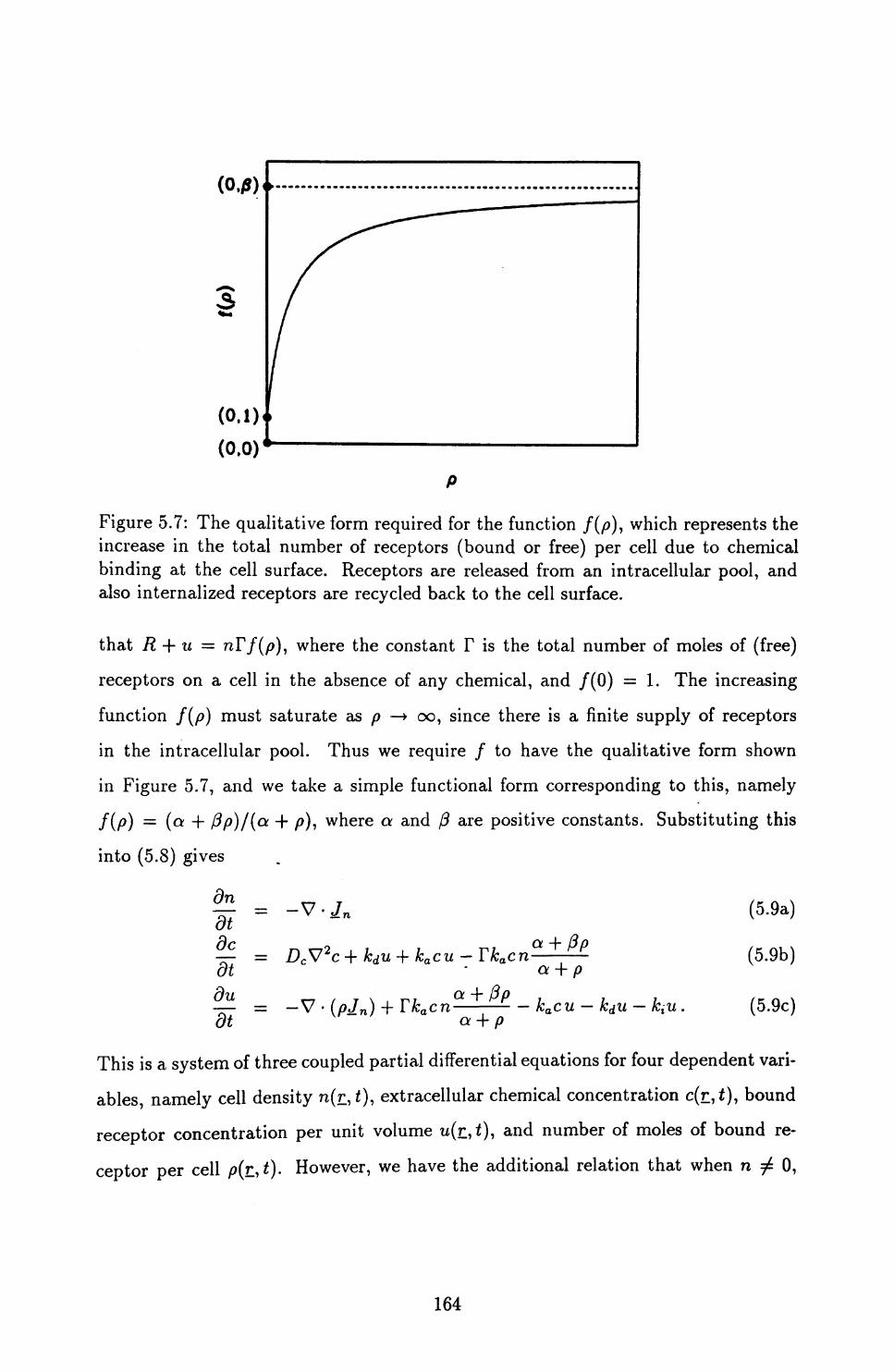
(0,0)

Figure 5.7: The qualitative form required for the function /(/?), which represents the increase in the total number of receptors (bound or free) per cell due to chemical binding at the cell surface. Receptors are released from an intracellular pool, and also internalized receptors are recycled back to the cell surface.

that R + u = nF/(/9), where the constant F is the total number of moles of (free)

receptors on a cell in the absence of any chemical, and /(O) = 1. The increasing

function f(p) must saturate as p —> oo, since there is a finite supply of receptors

in the intracellular pool. Thus we require / to have the qualitative form shown

in Figure 5.7, and we take a simple functional form corresponding to this, namely

f(p) = (a -f (3p)/(a + />), where a and /3 are positive constants. Substituting this

into (5.8) gives

dc n ^In = c^ = -v. a^

ka cu —

a + Pp

Pp

-kacu- kd u —

(5.9a)

(5.9b)

(5.9c)

This is a system of three coupled partial differential equations for four dependent vari­

ables, namely cell density rc(r, t), extracellular chemical concentration c(r, £), bound

receptor concentration per unit volume u(r, i), and number of moles of bound re­

ceptor per cell p(r_, t). However, we have the additional relation that when n ^ 0,

164

p = u/n; when n = 0, p is undefined. Therefore, when n / 0,

#/? 1 du u dn

_ c——•—— -kacp- (kd + J n a + p

using (5.9a) and (5.9c). Taking n, c and /> as the dependent variables, this implies

the model equations

dn _ .(5.10a)

kacnp — Tka cn ———— (5.10b)^"- Q -j- p

dp Jn'V/9 a + fip /KinN— ~ 1 Aca c———— — fca c/o — (A:^ + «,)/? when n =£ 0, (5.10c)6 n c*

where Jn is given in (5.7). The model can also be expressed with n, c and u as

dependent variables. However, the resulting conservation equation for u contains a

backwards diffusion term, which results in prohibitively large computational expense

of numerical solution when the model is applied to the Boyden chamber assay in this

form. If n(r, t) = 0, then /?(r, t) and its derivatives are undefined; the condition n > 0

then implies that Vn = 0. If in addition V2n = 0, then the value of p is immaterial;

otherwise, n ^ 0 (so that p is defined) at points arbitrarily close to r, and we define

P(T.-, t) by continuity.

5.3.1 Application to the Boyden chamber assayWe now consider applying this model to the Boyden chamber experiments of Sage

et al. (in preparation). As in the case of the Keller-Segel model discussed in the

previous section, the variable c is defined in both the wells and the filter, that is

— hL < x < hv + a, in the notation of Figure 5.1, while n is defined only within the

filter 0 < x < a. For /?, the strict inequality n(x, t) > 0 holds on 0 < x < a for all

t > 0, so that p is defined on 0 < x < a for alH > 0. To prove this, suppose that

on the contrary a sharp front of cell density exists within the filter, so that at times

£>0, ra = OonO<z< ((t) and n > 0 on ((t) < x < a, with ((t) a decreasing

165

function of time, not identically zero. Then n[£(t),t] = 0 for all t, so that

{A, + D,p(t(t),t}} gKW,*l , (5-11)§

using (5.10a); recall that p[£(t),t] is defined as linv^)* p(x, t), and we interpret

dp/dx[£(t),t] as a right-hand derivative. The requirement that n(x,t) > 0 for all x

and t implies that when £(*) > 0, dn/dx[((t),t] = 0, so that d2n/dx2 [£(t),t] = 0,

from (5.11). Equation (5.10a) then implies that dn/dt[£(t),t] = 0, so that n remains

zero at x = <f(t) for all t. Moreover, successive differentiation of (5.10a) with respect

to x the implies that as many spatial derivatives of n with respect to x as exist at

x = £(t) are zero; in particular, if n is infinitely differentiate with respect to x, then

n is identically zero on some neighbourhood of £(£), which contradicts the original

definition of £ . This phenomenon of the non-existence of sharp fronts is familiar from

the diffusion equation (see, for example, Haberman, 1987).

Therefore equations (5.10) apply on the whole of 0 < x < a for all t > 0. In the

well regions, the concentration of SPARC c satisfies the diffusion equation, dc/dt =

Dc d2 c/dx2 ; we require continuity of chemical flux, dc/dx, at the ends x = 0 and

x = a of the filter, with dc/dx = 0 at x = — /& L , hu + a. As in Section 5.2, we

take the boundary conditions satisfied by the cell density to be n = 0 at x = 0,

and n = l/Vceii at x = a, where Vcen is the volume of an endothelial cell. For /?,

our approximation that the cell density is constant on the top surface of the filter

implies that the bound receptor density there changes only as a result of association,

dissociation and internalization, so that p(l,t) satisfies

, 0 - [** + *f]p(i. 0 •at

As a cell emerges onto the lower surface of the filter, it moves rapidly away from the

pore, and becomes surrounded by molecules of SPARC. Since the pores represent only

about 1% of the total cross-sectional area of the filter, there are then no neighbouring

166

cells whose free receptors would compete for the binding of these SPARC molecules.

Therefore, differences in the number of bound receptors across the length of a cell

disappear as the cell emerges from the filter, so that dp/dx = 0 at x = 0.

5.3.2 Parameter valuesIn Section 5.2, we established the dimensional parameter values Dc = 1.4x 10~6cmas~1

and Vceii — 1000//m3 . We will determine the values of the transport coefficients D0 ,

DI and x by comparing the model predictions with the data of Sage et a/., but we

must first obtain estimates for the parameters fca , fc^, &,-, F, a and /?, which reflect

the number and kinetics of the chemical receptors on the cell surface. We are not

aware of any relevant quantitative data for the receptors to SPARC on endothelial

cells. However, Sklar et al. (1984) have made a detailed study of the dynamics of

the interaction between an N-formyl peptide and its receptors on human neutrophils.

They use fluoresceinated peptide, and investigate the receptor kinetics using a combi­

nation of fluorimetric and cytometric techniques; these two experimental procedures

are described in detail by Sklar et al. (1981) and Finney and Sklar (1983) respectively.

They find that the kinetics are highly temperature-dependent: for example, internal-

ization is essentially blocked at 4°C. However, at 37 °C, they find the rate constants to

be ka = 109 M- 1 min~ 1 , fc, = 0.24mm- 1 and kd = 0.35mm- 1 . For T, a and ft, recall

that F is the number of moles of (free) receptor on the cell surface in the absence

of chemical, while (3T is the upper limit on the total number of moles of receptor

(free or bound) on the cell surface, due to the finiteness of the intracellular pool of

receptors. Again, data for receptors to SPARC on endothelial cells is not available,

but unactivated neutrophils have about 3000 peptide receptors, and this can increase

to as much as 100,000 when the cells are exposed to a variety of stimuli (Devreotes

and Zigmond, 1988). Therefore, we take T = 3000/6.02 x 1023 = 4.98 x 10~21 mol and

ft = 100,000/3000 = 33|.

The presence of 100,000 peptide receptors on a neutrophil corresponds to all the

receptors in the intracellular pool being released to the surface. This state cannot

167

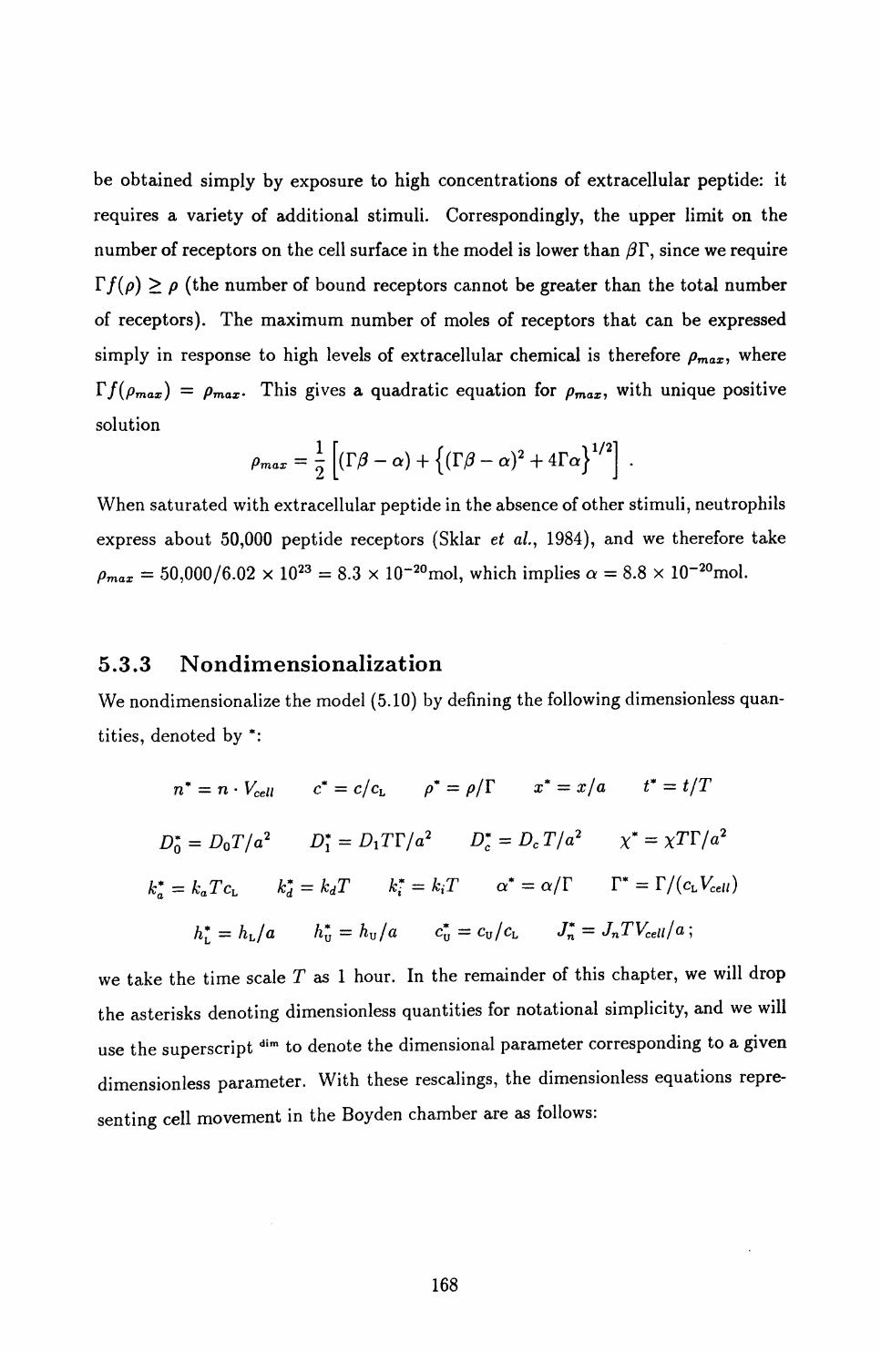
be obtained simply by exposure to high concentrations of extracellular peptide: it

requires a variety of additional stimuli. Correspondingly, the upper limit on the

number of receptors on the cell surface in the model is lower than /?F, since we require

Ff(p) > p (the number of bound receptors cannot be greater than the total number

of receptors). The maximum number of moles of receptors that can be expressed

simply in response to high levels of extracellular chemical is therefore />max , where

Ff(pmax) = pmax- This gives a quadratic equation for pmax , with unique positive

solution

/W* = \ [(Tft - a) + {(Tft - a)2 + 4ra}'/2] .

When saturated with extracellular peptide in the absence of other stimuli, neutrophils

express about 50,000 peptide receptors (Sklar et a/., 1984), and we therefore take

= 50,000/6.02 x 1023 = 8.3 x 10-20 mol, which implies a = 8.8 x 10-20mol.

5.3.3 NondimensionalizationWe nondimensionalize the model (5.10) by defining the following dimensionless quan­

tities, denoted by *:

n" = n • Vcen c* = C/CL p" = p/T x* = x/a f = t/T

0; = DoT/a2 D\ = ATT/a2 D*c = Dc T/a2 X * = X^/a2

k*a = ka TcL k*d = kdT k* = kiT a* = a/r P = r/(cL Vcen )

hi = hL /a h* = hv/a <% = CV /CL J* = JnTVceu/a ;

we take the time scale T as 1 hour. In the remainder of this chapter, we will drop

the asterisks denoting dimensionless quantities for notational simplicity, and we will

use the superscript dim to denote the dimensional parameter corresponding to a given

dimensionless parameter. With these rescalings, the dimensionless equations repre­

senting cell movement in the Boyden chamber are as follows:

168

Ono< * <1: = -

-T— oxdc

(5.12c)

where Jn = —(-Do + D\p}^- + Xn^~

On -/IL < x < 0

and !<*</>„: | = flcg. (5 .12d)

These equations are subject to the following end conditions:

At * = 0 : n = OonO<x<l, n = latx = l (5.13a)

/o = OonO<x<l (5.13b)

c=lon — ^ L < x < 1, c = cu onl<x</iu (5.13c)

At x = 0 : n = 0 (5.13d)

= 0 (5.13e)

continuous (5.13f)C/ vU

At x = 1 : n = 1 (5.13g)

(5.13h)a + /9

continuous (5.13i)

Before discussing the model solutions in detail, we investigate, in the next section,

methods of numerical solution. We will then obtain quantitative estimates for the

transport coefficients D0 , DI and x, using the experimental results of Sage et al. that

are illustrated in Figure 5.2. However, before presenting this work, we show the form

of the model solutions in Figures 5.8 and 5.9. We plot n, c and p against x at a selec­

tion of equally spaced times, for the parameter values discussed in Section 5.3.2 and

for the estimates of DOI D\ and x obtained in Section 5.5, with initial concentrations

169

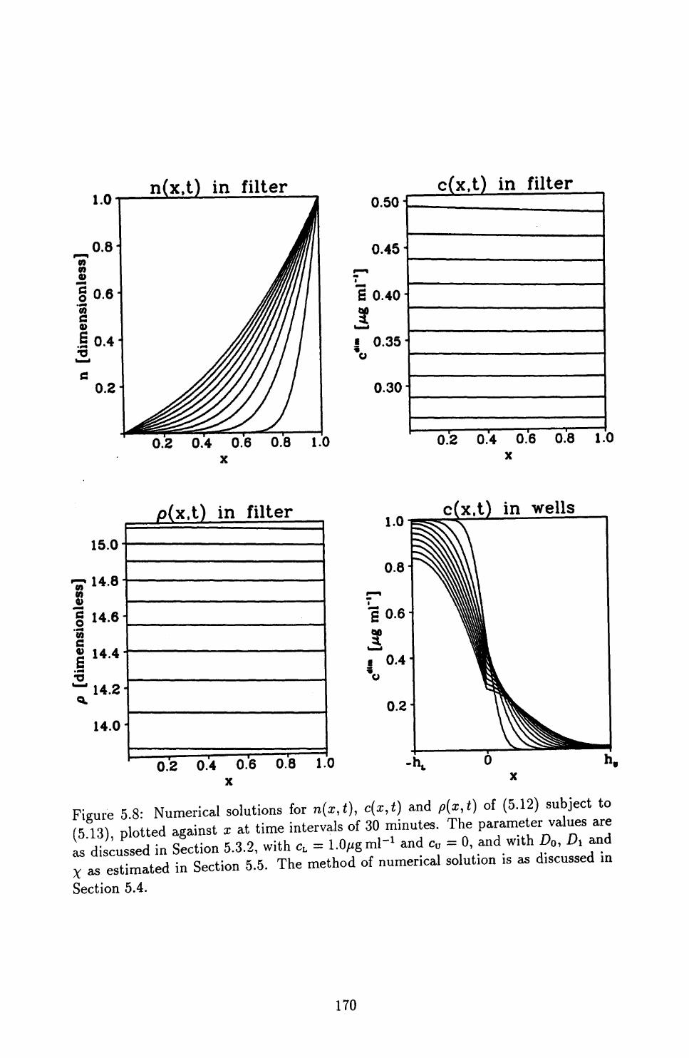
n(x,t) in filter

0.2 0.4 0.6 0.8 1.0

0.50-

0.45-

S 0.40 -I3!

• 0.35

0.30

c(x,t) in filter

0.2 0.4 0.6 0.8 1.0 x

15.0

m

14.6-1

14.4

14.2-

14.0

p(x,t) in filter c(x.t) in wells

0.2 0.4 0.6 0.8 1.0 x

Figure 58- Numerical solutions for n(x,t), c(x,t) and p(x,t) of (5.12) subject to (5 13), plotted against x at time intervals of 30 minutes. The parameter values are as discussed in Section 5.3.2, with CL = 1.0Mgml-' and e, = 0, and with D0 , A and x as estimated in Section 5.5. The method of numerical solution is as discussed in

Section 5.4.

170

1.0

0.8» «

nG 9)

04• «4 >*>^-o

0.2

n(x,t) in filter

0.2 0.4 0.6 0.8 1.0

0.95

• 0.90

0.85

0.80

0.75

c(x.t) in filter

0.2 0.4 0.6 0.8 1.0X

15.85

TP 15.80MJD

| 15.75

4)

3 15.70

15.65

/?(x,t) in filter in wells

0.2 0.4 0.6 0.8 1.0X

Figure 5.9: Numerical solutions for n(x,£), c(x,t) and p(x,t) of (5.12) subject to (5.13), plotted against x at time intervals of 30 minutes. The parameter values are as discussed in Section 5.3.2, with CL = cjim = 1.0/igml" 1 , and with D0 , DI and X as estimated in Section 5.5. The method of numerical solution is as discussed in Section 5.4.

171

of SPARC CL = l.O/igml" 1 , Cu = 0 and CL = cjim = LO/zgml" 1 respectively. In these

figures, it is not immediately clear that conditions (5.13e,f and i) are satisfied, but

this is confirmed by detailed numerical investigation. In both cases, a wave of cell

density moves through the filter during the experiment. The concentration of extra­

cellular SPARC decreases with time due to rapid binding and internalization of bound

receptors at the cell surface, and after an initial rapid rise from zero, the number of

these bound receptors per cell also decreases because dissociation and internalization

of the receptor-chemical complex occur slightly more rapidly than its association. In

both cases, the spatial gradients in both extracellular chemical concentration and

bound receptors per cell are quite small.

5.4 Numerical Methods of SolutionAlthough (5.12) subject to (5.13) is essentially a system of three coupled reaction-

diffusion equations, with given initial and boundary conditions, the equations are of

a rather non-standard form, so that particular care must be applied when solving the

system numerically. For a system of reaction-diffusion equations

methods of numerical solution can be broadly divided into three types: explicit, semi-

implicit and fully implicit. Denoting the solution at space node i and time step j by

£/:•, the corresponding discretizations are:

17 i- •* ~ n i- . F(lfiExplicit: —— — —— = JJv • ———— T~i ———— ]+£.(LLiSt — 2rr

n • • r •* » ~~— i A\*~fn \Semi-implicit: —— j- —— = diag(^u) • I ————— —

TTJ __ or/J _i_ TJ~m 7' -1 + £(K) (5.i4b)ox

i -\-I7H • r •* « « Fully implicit: —— — ——

where 8x is the space node separation, 6t is the time step, and diag(M) denotes the

matrix of the diagonal entries of M, with all off-diagonal entries zero. These categories

172

refer to the spatial discretization of the equations; here we are, for simplicity, using an

Eulerian discretization in time. In Chapter 1, we solved the reaction-diffusion systems

(1.1), (1.2) and (1.6) numerically using the method of lines and Gear's method. This

is an explicit method, but in contrast to (5.14a), the time discretization corresponds

to solving the system of ordinary differential equations

using Gear's method, which is a numerical scheme based on the Adams- Bashfort h-

Moulton method, and is very much more stable than the simpler Euler scheme (Lam­

bert, 1973); here U{(t) denotes the solution at space node « and time t.

We have used each of the three methods (5.14a,b,c) of numerical solution for (5.12)

subject to (5.13). As expected intuitively, the time step St required for convergence

with a given space mesh is smaller for (5.14b) than for (5.14c), and smaller still

for (5.14a); this is the well-known phenomenon that feedback stabilizes numerical

methods of solution (see, for example, Haberman, 1987). However, numerical solution

of the nonlinear algebraic equations (5.14c) for {U^ , z = 1, . . . ,nspace } in terms

of {U.\ii — 1, • • • , ^space} required a great deal more processing time than for the

linear equations (5.14b), so that the semi-implicit scheme was the most efficient of

the three methods; here nspace denotes the number of nodes in the space mesh. In

the remainder of this section, we present a detailed investigation of the space node

separation Sx and the time step St required for convergence of the semi-implicit

method of solution. Throughout, we use the dimensionless transport coefficients

DQ = 3.6 x 10~3 , DI = 9.7 x 10~4 , x — 3.6; the trends we will discuss are the same

for a wide range of values of these parameters.

Since the initial conditions for n and c are discontinuous, the solutions of (5.12)

subject to (5.13) change rapidly at small times t. Correspondingly, the time step

required to give convergence of the semi-implicit method during the early part of the

experiment is very small, as illustrated in Table 5.1. In this table we list, for the cases

c — 0 and cdim = CL , and for a range of values of CL , a time step such that the method

converges for that time step, but fails to converge when twice that time step is used.

173

cL [/zgml l ]0.030.031.01.0

30.030.060.060.0

^[//gml-1 ]0.00.030.01.00.0

30.00.0

60.0

A time step giving convergence1.0 x 10~44.5 x 10-51.0 x 10~65.0 x 10-77.0 x 10~85.0 x 10-84.0 x 10-83.0 x 10-8

Time of onset of instability when twice that time step is used

8.0 x 10~43.6 x 10-42.9 x 10-31.3 x ID-37.0 x 10~73.0 x 10-73.2 x 10~71.8 x 10-7

Table 5.1: The time step required for initial convergence of the semi-implicit method (5.14b) for numerical solution of (5.12) subject to (5.13). The parameter values are as discussed in Section 5.3.2, with Z)0 = 3.6 x 10~3 , Dl = 9.7 x 10~4 and x = 3.6. For each value of c l̂tn and CL , we give a time step such that the method converges when that time step is used, but fails to converge when twice that time step is used. We also give the time of the onset of numerical instability in the latter case, which we define as the first time at which one of n, c or p is negative. In each case, a full numerical blow up ensues.

We also give the dimensionless time at which the numerical method becomes unstable

in the latter case. Here we define the onset of instability as the time at which one of

the dependent variables n, c or p becomes negative; in each case, a full numerical blow

up ensues. The time step required for convergence decreases markedly as CL increases,

causing the dimensionless parameters ka and T to increase and decrease respectively.

We initially suspected that this decrease was due to changes in the value of p: as

discussed in Section 5.5, the value of p increases with CL , so that the effective cellular

diffusion coefficient (D0 + Dip) increases, and the effective chemotaxis coefficient

Xdp/dx also changes. These variations in the effective transport coefficients might

be expected to affect stability, since such changes are known to control the stability

of the explicit method (5.14a) of numerical solution (see page 49). However, careful

investigation has shown that in this case the major factor controlling stability is the

values of the dimensionless parameters T and fc0 , which depend on CL , rather than

the values of the transport coefficients.

After rapid initial changes, the solution of (5.12) subject to (5.13) changes more

174

cj/zgml- 1 ]

0.030.031.01.0

30.030.060.060.0

cj-^gml-1 ]

0.00.030.01.00.0

30.00.0

60.0

A value of s\ giving convergence

7.0 x 10~33.5 x 10-38.7 x 10~48.7 x 10~43.1 x 10~41.6 x 10~41.0 x 10-45.0 x 10-5

Time of onset of instability when twice that value is used

9.0 x 10~22.3 x 10-22.7 x 10-32.5 x 10~3

0.320.310.4970.6135

Table 5.2: The value of the time step parameter s\ required for convergence up to times t ^> SQ/SI of the semi-implicit method (5.14b) for numerical solution of (5.12) subject to (5.13), when the time step is given by (5.15). The parameter values and the value of s0 are as in Table 5.1. For each value of cjim and CL , we give a value of s\ such that the method converges when that value is used, but fails to converge when twice that value is used. We also give the time of the onset of numerical instability in the latter case, which we define as the first time at which one of n, c or p is negative. In each case, a full numerical blow up ensues.

slowly with time. We exploited this in our numerical solutions by using a time step which increased with time, namely

sit . (5.15)

The values of s0 required for initial convergence as CL and cv vary are simply the time steps listed in Table 5.1. In Table 5.2 we list, again for the two cases GU = 0 and 4im = CL , and for a range of values of CL , a value of si giving convergence (when s0 is sufficiently small), but such that convergence fails when twice that value is used.

This method of increasing the time step as t increased was very successful in reducing the computational expense of solution. However, the time step cannot be increased indefinitely, so that with a time step of the form (5.15), the numerical scheme (5.14b) becomes unstable for sufficiently large t. We therefore used a time

step of the form8t = min{s0 + sit,s2 }. (5.16)

The values of s2 required for convergence in the various cases are listed in Table 5.3: for small values of CL , introduction of an upper limit s2 on the time step was not

175

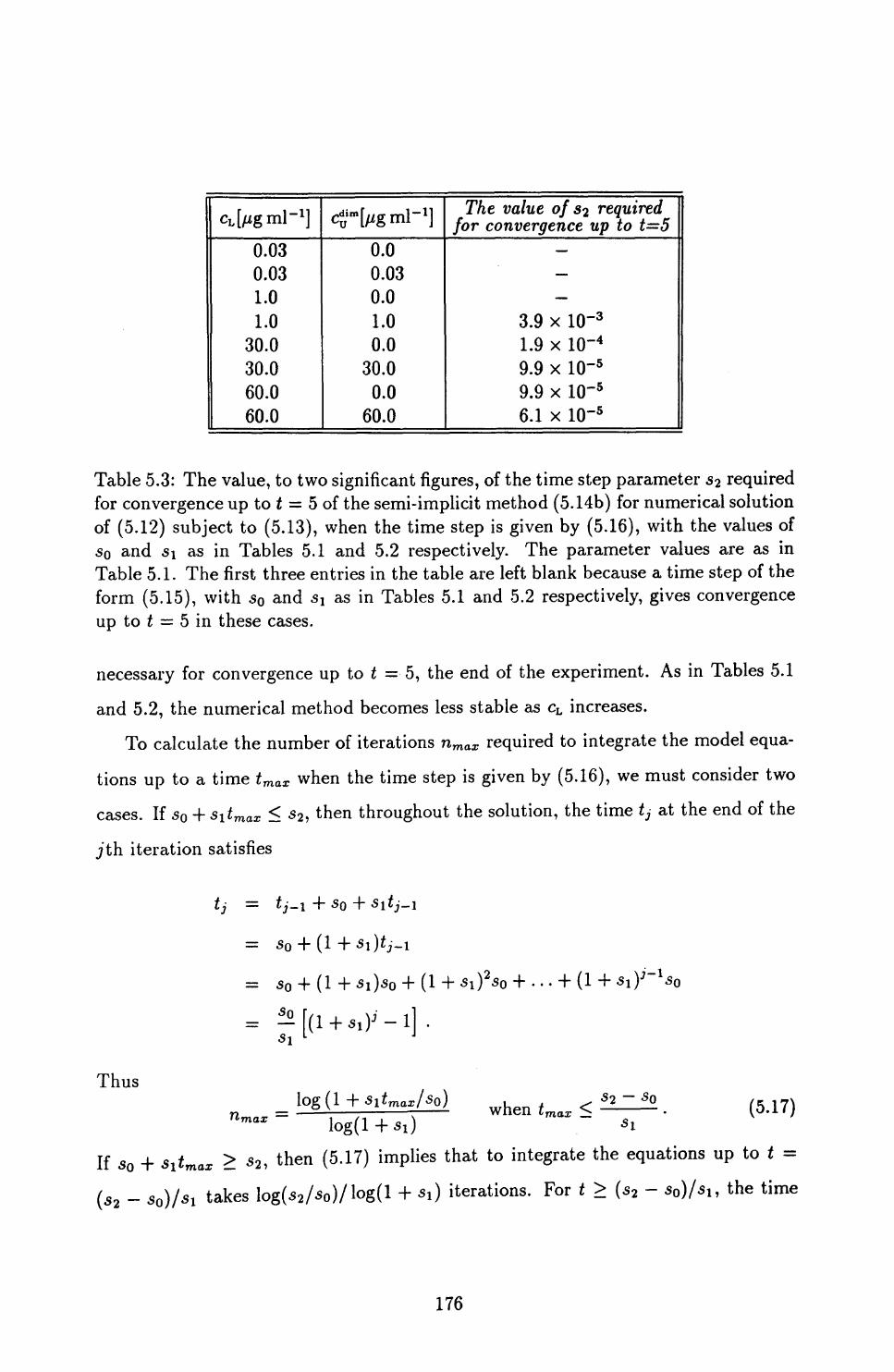
CL^gml- 1 ]

0.030.031.01.0

30.030.060.060.0

cj-^gml-1 ]

0.00.030.01.00.0

30.00.0

60.0

The value of s? required for convergence up to t=5

———

3.9 x lO'31.9 x 10-49.9 x 10~59.9 x 10-56.1 x 10-5

Table 5.3: The value, to two significant figures, of the time step parameter ^2 required for convergence up to t = 5 of the semi-implicit method (5.14b) for numerical solution of (5.12) subject to (5.13), when the time step is given by (5.16), with the values of SQ and si as in Tables 5.1 and 5.2 respectively. The parameter values are as in Table 5.1. The first three entries in the table are left blank because a time step of the form (5.15), with SQ and Si as in Tables 5.1 and 5.2 respectively, gives convergence up to t = 5 in these cases.

necessary for convergence up to t =• 5, the end of the experiment. As in Tables 5.1

and 5.2, the numerical method becomes less stable as CL increases.

To calculate the number of iterations nmax required to integrate the model equa­

tions up to a time tmax when the time step is given by (5.16), we must consider two

cases. If sQ + Sitmax < s2 , then throughout the solution, the time tj at the end of the

jth iteration satisfies

tj = tj-i -\~SQ-\-

= SQ + (I + Si)tj-i

= S0 + (l+Si)s0 + (l + + . . • + (1 + Si)3 ' 1 SQ

Si

Thus

nmax\Og(l+Sitmax/S0 )= ——:—7-———:—— wnen t mar ^

so (5.17)

If s0 + sitmax > «2, then (5.17) implies that to integrate the equations up to t =

(S2 _ So)/3l takes Iog(s2 /s0 )/log(l + *i) iterations. For t > (s2 - a0)/*i, the time

176

^[//ginl-1 ]

0.030.031.01.0

30.030.060.060.0

^-[//grnl-1 ]

0.00.030.01.00.0

30.00.0

60.0

Number of iterations to integrate up to t=5

84017079634

104394860091705

118653214330

Table 5.4: The number of iterations required to integrate the model equations (5.12) subject to (5.13) up to t = 5, the dimensionless duration of the experiments of Sage et al. The listed values are calculated using (5.17) and (5.18), with the values of the time step parameters SQ, s\ and 52 as in Tables 5.1, 5.2 and 5.3. Each iteration takes an average of about 0.05 seconds of processing time on a 6 MIPS machine.

step has the constant value ^2, so that11".

= — \tmax ~ S2 I

^£0 + •og^.i when tm_ > .,^.0 (5 lg) si J log(l -f Si) si

In Table 5.4 we list the values of nmax corresponding to tmax — 5, the dimensionless duration of the experiments of Sage et a/., as implied by the values of SQ, s\ and ^2 given in Tables 5.1, 5.2 and 5.3 respectively. The required number of iterations, and thus the computational expense of solution, increases markedly with CL .

In our numerical simulations, we used a space mesh which was uniform in the filter region 0 < x < 1, and which in the well regions increased in a geometric progression, moving away from the filter. In the simulations used to determine Tables 5.1, 5.2 and 5.3, we used ra/ = 60 and nw = 500, where rc/ and nw are the number of space nodes in the filter and well regions respectively. However, the values of the time step parameters s0 , -$1 and s2 required for convergence are very insensitive to variations in n/ and nw , and the values listed in Tables 5.1, 5.2 and 5.3 give convergence for values of nj and nw as large as 300 and 2000 respectively. This insensitivity is in marked contrast to the explicit method of numerical solution (5.14a), which we used in Sections 2.2 and 2.3; for the explicit method, convergence requires the time step

to be less than a critical value, which is proportional to the square of the space node

177

nf60

120240480960

/V it fnr f^im — r, •' v cej/ 1*-'i *"\j HJ

23.3023.2223.2023.1823.17

Ncen for Cy

130.1127.4125.2123.3122.2

= 0

Table 5.5: The effect of varying the space node separation on the value of Nceii, the model prediction of the number of cells per unit area passing through the lower surface of the filter during the experiment. For CL = l.O/zgml"1 , with both cv = 0 and cjim = CL , we list the value of JVce//, calculated using (5.19), that is predicted by the semi-implicit method (5.14b) of numerical solution, for a range of values of n/, the number of space nodes in the filter region. The parameter values are as in Table 5.1, with nw = 500 in each case.

separation (see page 49).

Increasing the values of n/ and nw above 60 and 500 respectively has a negligible effect on the numerical solutions for n, c and p. However, the model predictions of Nceii, the number of cells per unit area passing through the lower surface of the filter during the experiment, decreases slightly as n/ increases. The extent of this decrease depends on cv and CL , and is illustrated in Table 5.5 for a particularly sensitive case, namely CL = l.O^gml" 1 , c0 = 0, and for comparison, also for the case cL = cjim = 1.0/igml" 1 . As a compromise between computational expense and accuracy, we have used n/ = 240 and nw = 300 in the simulations discussed in the remainder of the chapter. The results given in Table 5.5 suggest that as CL varies, the model prediction of Nceu with n/ = 240 is at worst within a few percent of the

true value.

5.5 Application of the Improved Model to the Boyden Chamber Assay

In the previous two sections, we have developed a model for chemically controlled cell movement based on chemical-receptor interactions on the cell surface, and we

178

have discussed in detail a semi-implicit method for numerical solution of the model

equations when applied to the Boyden chamber assay. We now use the data of Sage

et a/., illustrated in Figure 5.2, to obtain quantitative estimates for the transport

coefficients D0 > D\ and x; we have obtained estimates for the other parameter values,

based on biological data, in Section 5.3.2.

The dimensionless flux of cells through the lower surface of the filter is, for the

improved model (5.12), (D0 + Dip\x-0 ) • (dn/dx)\x-0. Thus the model prediction of

the number of cells passing onto the lower surface of the filter per unit dimensional

area during the 5 hours of the experiment is

a f5 f n , n i \ dn (D0 + Dip\x=0 ) dt. (5.19)x=0

T/ / V U ' ^iri*=U/ QVce// JO (/X

This expression, together with the numerical method of solution discussed in the

previous section, enables us to predict the value of Nceii for given values of A), D\, \i

Cu and CL . However, fitting these predictions to all the experimental data illustrated

in Figure 5.2 would be computationally infeasible (see Table 5.4). Rather, we use

the estimate for DQ obtained as Dn (Q) in Section 5.2: when there is no chemical

present, (5.12) and the simple model (5.3) both reduce to a linear diffusion equation

for n. We then estimate D\ and x using the results obtained experimentally by Sage

et al. for the number of cells on the lower surface of the filter after 5 hours, when

CL = 0.5/jg ml" 1 , GU = 0, and when CL = cjiin = 0.5^g ml" 1 ; we select 0.5//g ml" 1 as the

concentration giving the greatest difference between the cases cy = 0 and cjlm = CL in

the experiments of Sage et al This approach gives two coupled nonlinear algebraic

equations to be solved for D\ and \.

The estimates for the dimensional parameter values obtained in this way are

D$m = 6.5 x K

D*m = 9.9 x 109cm2s~ 1 mor 1

dim = 1.5 x lO

With these values, the variation in Nceii with CL in the two cases cv = 0 and cjim = CL ,

as predicted by the model, is shown in Figure 5.10. In both cases, the dose-response

179

600

0.015 0.1 1 10 30 Cone, of SPARC, ct [^g ml"1 ]

Figure 5.10: The variation with CL of the model prediction of the number of cells per unit area on the lower surface of the filter after 5 hours. The parameter values are as discussed in Section 5.3.2, with the estimates for D0 , DI and \ that are described in the text. The method of numerical solution of (5.12) subject to (5.13) is discussed in Section 5.4, and the number of cells per unit area on the lower surface of the filter at the end of the experiment is calculated using (5.19). For clarity, we plot CL on a logarithmic scale.

curves are bell-shaped, and this shape of curve has been found in Boy den chamber

assays for a wide range of chemicals and cell types (see Bignold, 1988b, for references).

For low chemical concentrations, the response is low due to the small number of

bound receptors per'cell, so that the chemokinetic response is low. In contrast,

for high chemical concentrations, the cells are saturated with extracellular chemical,

so that the spatial variation in the number of bound receptors per cell, and thus

the chemotactic response, is low. In comparison to the case cv = 0, when cjim =

CL the number of bound receptors per cell is larger due to the higher extracellular

chemical concentration in the filter, but the consequent increase in chemokinetic

response is smaller than the reduction in chemotactic response, which results from

the lower spatial gradient in extracellular chemical concentration and thus in the

number of bound receptors per cell. These trends are illustrated in Figures 5.11,

5.12 5.13 and 5.14, in which we plot the solutions of (5.12) subject to (5.13) for

CL = O.OS^gml" 1 and CL = SO^gml" 1 , with c0 = 0 and cjim = CL in both cases.

180

n(x,t) in filter

0.2 0.4 0.6 0.8 1.0

0.014

0.013

C 0.012 6

0.011

j 0.010y

0.009 •

0.008 •

c(x.t) in filter

0.2 0.4 0.6 0.8 1.0X

0.9-

0.8"c

I 0.7c0)

I 0.6

0.5

0.4-

p(x,t) in filter

0.2 0.4 0.6 0.8 1.0X

0.030c(x t t) in wells

Figure 5.11: Numerical solutions for n(x,t), c(x,t) and p(x,t) of (5.12) subject to (5.13), plotted against x at time intervals of 30 minutes. The parameter values are as in Figure 5.10, with CL = 0.03/zgml- 1 and c0 = 0.

181

n(x.t) in filter

0.2 0.4 0.6 0.8 1.0

0.028

0.026 ^

c(x,t) in filter

0.024

0.022

0.020

0.018

0.016

0.014

0.2 0.4 0.6 0.8 1.0 x

p(x.t) in filter2.75

^ 2.50 • *7 8 2.25 •

| 2.00-

1 1 -752, 1.50- ^ 1.25-

i.oo-0.5 1.'

x

0.030

0.028

0.026

c(x,t) in wells

Figure 5 12- Numerical solutions for n(x,t), c(x,t) and p(x,t) of (5.12) subject to (5.13), plotted against x at time intervals of^O minutes. The parameter values are as in Figure 5.10, with CL = <"• = O.-

182

n(x,t) in filter

0.2 0.4 0.6 0.8 1.0

15.2

15.1

15.0

• 14.9-

14.8

14.7 ^

c(x.t) in filter

0.2 0.4 0.6 0.8 1. x

16.6130

09 9)

o 16.612501e

2, 16.6120

16.6115-

p(x,t) in filter c(x,t) in wells

0.2 0.4 0.6 0.8 1.0X

Figure 5.13: Numerical solutions for n(x,t), c(x,t) and p(x,t) of (5.12) subject to (5.13), plotted against x at time intervals of 30 minutes. The parameter values are as in Figure 5.10, with CL = SO^gml" 1 and cv = 0.

183

n(x,t) in filter

29.95

0.2 0.4 0.6 0.8 1.0

29.75 •

c(x.t) in filter

0.2 0.4 0.6 0.8 1.0 x

16.639801

16.63975-

J2 16.63970-o 'w

§ 16.63965-1 6

.!§•T 16.639601

16.63955-

p(x.t) in filter30.00

29.95 •

u? 29.90s^ 29.85B

29.80

29.75 H

0.2 0.4 0.6 0.8 1.0 x

c(x,t) in wells

Figure 5.14: Numerical solutions for n(x,t), c(x,t) and p(x,t) of (5.12) subject to (5.13), plotted against x at time intervals of 30 minutes. The parameter values are as in Figure 5.10, with CL = cjim = 30//g ml' 1 .

184

6 175-

~15<^0

S 125

3S 100-cu 75* 50-

J2fl) £t^jo

12345 Time [hours]

Figure 5.15: The model prediction of the increase with time of the number of cells per unit area on the lower surface of the filter. The parameter values are as in Figure 5.10, and the number of cells per unit area on the lower surface of the filter is calculated as (a/Vceu) /0f (A) + D\p\x=o) • (dn/dx)\x-o dt', which corresponds to the expression (5.19) for the number at t = 5.

These should be compared with the solutions for the cases CL = 1.0/Jgml"" 1 , cv = 0

and CL = cjim = l.O/xgml" 1 , which are illustrated in Figures 5.8 and 5.9 respectively.

The number of cells on the lower surface of the filter increases gradually during the

experiment. The model prediction of this increase is illustrated in Figure 5.15 for

the case CL = 1.0/igml" 1 , cv = 0, and the shape of the curve is qualitatively similar

for all the values of cv and CL we have considered. Quantitative data to which such

curves could be compared is not currently available.

The experimental results of Sage et al. that are illustrated in Figure 5.2 are

only preliminary results. Therefore, the differences between the model predictions

illustrated in Figure 5.10 and the experimental results in Figure 5.2 can to some

extent be attributed to experimental inaccuracies: additional sets of experiments are

currently in progress. However, another major factor responsible for these differences

is that the kinetic parameters and receptor numbers will not be exactly the same

for the endothelial cell-SPARC system and the leukocyte-peptide system. Thus our

estimates for fa, fa, fc, F, a and /?, based on data for the latter system, are only semi-

quantitative when applied to the experiments of Sage et al. Experimental work to

185

determine quantitative data on the receptors to SPARC on endothelial cells is currently

in progress (Helene Sage, personal communication, 1990).

5.6 ConclusionsIn this chapter, we have developed a new model for chemically controlled cell move­

ment. In contrast to the highly successful model of Keller and Segel (1971a,b), our

model reflects the receptor based mechanisms that are responsible for chemotaxis

and chemokinesis in eukaryotic cells. We are therefore able to predict the bell-shaped

dose-response curves observed experimentally, without externally specifying the de­

pendence of the transport coefficients on extracellular chemical concentration. Using

the data of Sage et al. (in preparation) on the movement of bovine aortic endothelial

cells in response to concentration gradients of SPARC in the Boyden chamber assay,

we have quantitatively estimated the values of the transport coefficients in our model

for this cell-chemical system; we were able to estimate the other model parameters

from data in the biological literature.

The movement of endothelial cells in response to concentration gradients of regu­

latory chemicals such as SPARC is an important aspect of the process of angiogenesis,

in which a dense capillary network enters the granulation tissue of a healing wound.

Our model could therefore be used in a study of angiogenesis, and it is also relevant to

other processes in which cell influx into the wound space is mediated by chemotactic

and chemokinetic factors, in particular the influx of white blood cells during the early

"inflammation" phase of healing, and the invasion of the wound space by fibroblasts

during the formation of granulation tissue.

The complex mechanisms responsible for mammalian wound healing raise many

biological questions that are amenable to theoretical investigation. In this thesis, we

.have developed and analysed models relevant to three aspects of the healing process:

adult epidermal wound healing, embryonic epidermal wound healing, and chemically

controlled cell movement. We have made a number of biologically testable predictions,

and the work is relevant to both experimental and theoretical cell biologists.

186

References

Alberts, B., Bray, D., Lewis, J., Raff, M., Roberts, K., Watson, J. D.: The molecular

biology of the cell. Garland Publ. Inc., New York (1989).

Albrecht-Buehler, G.: Role of cortical tension in fibroblast shape and movement. Cell

Motil. 7: 54-67 (1987).

Arcuri, P. A.: Reaction diffusion mechanisms for biological pattern formation. D.Phil,

thesis, University of Oxford (1984).

Aronson, D. G., Cafferelli, L. A., Kamin, S.: How an initially stationary interface

begins to move in porous medium flow. SIAM J. Math. Anal. 14: 639-658 (1983).

Barnes, D.: Growth factors involved in the repair process: an overview. Meth. Enzy-

mol. 163: 707-715 (1988).

Barrow, G. M.: Physical chemistry for the life sciences. McGraw-Hill Inc., New York

(1981).

Bereiter-Hahn, J.: Epidermal cell migration and wound repair. In: Bereiter-Hahn, J.,

Matoltsy, A. G., Richards, K. S. (eds.) Biology of the integument, vol. 2: vertebrates.

Springer-Verlag, Berlin, pp. 443-471 (1986).

Berg, 0. G., Von Hippel, P. H.: Diffusion-controlled macromolecular interactions.

Ann. Rev. Biophys. Biophys. Chem. 14: 131-160 (1985).

Beyer W. H. (ed.): CRC standard mathematical tables, 26th Edition. CRC Press

Inc., Boca Raton, Florida, USA (1981).

187

Bignold, L. P.: Chemotaxis and chemokinesis of neutrophils: a reply. J. Immunol.

Meth. 110: 145-148 (1988a).

Bignold, L. P.: Measurement of chemotaxis of polymorphonuclear leukocytes in vitro.

J. Immunol Meth. 108: 1-18 (1988b).

Bonder, E. M., Mooseker, M. S.: Cytochalasin B slows but does not prevent monomer

addition at the barbed end of the actin filament. J. Cell Biol 102: 282-288 (1986).

Boyden, S. V.: The chemotactic effect of mixtures of antibody and antigen on poly­

morphonuclear leukocytes. J. Exp. Med. 115: 453-466 (1962).

Brugal, G., Pelmont, J.: Existence of two chalone-like substances in intestinal extract

from the adult newt, inhibiting embryonic intestinal cell proliferation. Cell Tissue

Kinet. 8: 171-187 (1975).

Buettner, H. M., Lauffenburger, D. A., Zigmond, S. H.: Measurement of leukocyte

motility and chemotaxis parameters with the Millipore filter assay. J. Immunol.

Meth. 123: 25-37 (1989a).

Buettner, H. M., Lauffenburger, D. A., Zigmond, S. H.: Cell transport in the Millipore

filter assay. Am. Inst. Chem. Eng. J. 35: 459-465 (1989b).

Canosa, J.: On a nonlinear diffusion equation describing population growth. IBM J.

Res. Dev. 17: 307-313 (1973).

Carson, M., Weber, A., Zigmond, S. H.: An actin-nucleating activity in polymor­

phonuclear leukocytes is modulated by chemotactic peptides. J. Cell Biol. 103:

2707-2714 (1986).

Charnick, S. B., Lauffenburger, D. A.: Mathematical analysis of cell-target encounter

rates in three dimensions. Biophys. J. 57: 1009-1023 (1990).

188

Chen, W.: Mechanism of retraction of the trailing edge during fibroblast movement.

J. Cell Biol 90: 187-200 (1981).

Citi, S., Kendrick-Jones, J.: Regulation of non-muscle myosin structure and function.

Bioessays 7: 155-159 (1987).

Clark, R. A. F.: Overview and general considerations of wound repair. In: Clark,

R. A. F., Henson, P. M. (eds.) The molecular and cellular biology of wound repair.

Plenum press, New York, pp. 3-34 (1988).

Clark, R. A. F.: Wound repair. Curr. Op. Cell Biol. 1: 1000-1008 (1989).

Coffey, R. J., Derynck, R., Wilcox, J. N., Bringman, T. S., Goustin, A. S., Moses, H.

L., Pittelkow, M. R.: Production and auto-activation of transforming growth factor-a

in human keratinocytes. Nature 328: 817-820 (1987).

Compton, C. C., Gill, J. M., Bradford, D. A., Regauer, S., Calico, C. G., O'Conner,

N. E.: Skin regenerated from cultured epithelial autografts on full-thickness burn

wounds from 6 days to 5 years after grafting. A light, electron microscope and

immunohistochemical study. Lab. Invest. 60: 600-612 (1989).

Cooper, J. A.: Effects of cytochalasin and phalloidin on actin. J. Cell Biol. 105:

1473-1478 (1987).

Courant, R., Hilbert, D.: Methods of mathematical physics. Interscience, New York

(1962).

Crosson, C. E., Klyce, S. D., Beuerman, R. W.: Epithelial wound closure in the

rabbit cornea. Invest. Ophthalmol. Vis. Sci. 27: 464-473 (1986).

Danio S., Friend, J., Throft, R. A.: Conjunctival epithelium in healing of corneal

epithelial wounds. Invest. Ophthalmol. Vis. Sci. 28: 1445-1449 (1987).

189

DeBiasio, R. L., Wang, L. L., Fisher, G. W., Taylor, D. L.: The dynamic distribution

of fluorescent analogues of actin and myosin in protrusions at the leading edge of

migrating Swiss 3T3 fibroblasts. J. Cell Biol. 107: 2631-2645 (1988).

Dennerll, T. J., Joshi, H. C., Steel, V. L., Buxbaum, R. E., Heidemann, S. R.: Tension

and compression in the cytoskeleton of PC-12 neurites II: quantitative measurements.

J. Cell Biol. 107: 665-674 (1988).

Devreotes, P. N., Zigmond, S. H.: Chemotaxis in eukaryotic cells: a focus on leuko­

cytes and Dictyostelium. Ann. Rev. Cell Biol. 4: 649-686 (1988).

Dvorak, H. F., Kaplan, A. P., Clark, R. A. F.: Potential functions of the clotting

system in wound repair. In: Clark, R. A. F., Henson, P. M. (eds.) The molecular

and cellular biology of wound repair. Plenum Press, New York, pp. 57-86 (1988).

Eisinger, M., Sadan, S., Soehnchen, R., Silver, I. A.: Wound healing by epidermal-

derived factors: experimental and preliminary chemical studies. In: Barbul, A.,

Pines, E., Caldwell, M., Hunt, T. K. (eds.) Growth factors and other aspects of

wound healing. Alan R. Liss Inc., New York, pp. 291-302 (1988a).

Eisinger, M., Sadan, S., Silver, I. A., Flick, R. B.: Growth regulation of skin cells

by epidermal cell-derived factors: implications for wound healing. Proc. Natl. Acad.

Sci. USA 85: 1937-1941 (1988b).

Elgjo, K., Reichelt, K. L., Edminson, P., Moen, E.: Endogenous peptides in epidermal

growth control. In: Baserga, R., Foa, P., Metcalf, D., Polli, E. E. (eds.) Biological

regulation of cell proliferation. Raven Press, New York, pp. 259-265 (1986a).

Elgjo, K., Reichelt, K. L., Hennings, H., Michael, D., Yuspa, S. H.: Purified epidermal

pentapeptide inhibits proliferation and enhances terminal differentiation in cultured

mouse epidermal cells. J. Invest. Dermatol. 87: 553-558 (1986b).

190

Elson, E. L.: Cellular mechanics as an indicator of cytoskeletal structure and function.

Ann. Rev. Biophys. Biophys. Chem. 17: 397-430 (1988).

Engel, J., Taylor, W., Paulsson, M., Sage, H., Hogan, B.: Calcium binding do­

mains and calcium-induced conformational transition of SPARC/BM-40/Osteonec-

tin, an extracellular glycoprotein expressed in mineralized and nonmineralized tissues.

Biochem. 26: 6958-6965 (1987).

Faulstich, E., Trischmann, H., Mayer, D.: Preparation of trimethylrhodaminyl-phal-

loidin and uptake of the toxin into short-term cultured hepatocytes by endocytosis.

Exp. Cell Res. 144: 73-82 (1983).

Ferry, J. D.: Viscoelastic properties of polymers. John Wiley and Sons, New York

(1980).

Finney, D. A., Sklar, L. A.: Ligand/receptor internalization: a kinetic, flow cyto-

metric analysis of the internalization of N-formyl peptides by human neutrophils.

Cytometry 4: 54-60 (1983).

Fisher, E. S., Lauffenburger, D. A.: Mathematical analysis of cell-target encounter

rates in two dimensions. The effect of chemotaxis. Biophys. J. 51: 705-716 (1987).

Fletcher, M. P., Gallin, J. I.: Degranulating stimuli increase the availability of re­

ceptors on human neutrophils for the chemoattractant f-Meu-Leu-Phe. J. Immunol.

124: 1585-1588 (1980).

Folkman, J., Moscona, A.: Role of cell shape in growth control. Nature 273: 345-349

(1978).

Forrest, L.: Current concepts in soft connective tissue wound healing. Br. J. Surg.

70: 133-140 (1983).

191

Forscher, P., Smith, S. J.: Actions of cytochalasins on the organization of actin

filaments and microtubules in a neuronal growth cone. J. Cell Biol. 107: 1505-1516

(1988).

Frantz, J. M., Dupuy, B. M., Kaufman, H. E., Beuerman, R. W.: The effect of

collagen shields on epithelial wound healing in rabbits. Am. J. Ophthalmol. 108:

524-528 (1989).

Fremuth, F.: Chalones and specific growth factors in normal and tumor growth. Ada

Univ. Carol. Monogr. 110 (1984).

Ftirie, B., Furie, B. C.: The molecular basis of blood coagulation. Cell 53: 505-518

(1988).

el-Ghorab, M., Capone, A., Underwood, B. A., Hatchell, D., Friend, J., Throft, R.

A.: Response of ocular surface epithelium to corneal wounding in retinol-deficient

rabbits. Invest. Ophthalmol. Vis. Sci. 29: 1671-1676 (1988).

Goldbeter, A., Koshland, D. E.: Simple molecular model for sensing and adaptation

based on receptor modification with application to bacterial chemotaxis. J. Mol.

Biol. 161: 395-416 (1982).

Gordon, S.: The biology of the macrophage. J. Cell Sci. Suppl. 4: 267-286 (1986).

Grotendorst, G. R., Grotendorst, C. A., Gilman, T.: Production of growth factors

(PDGF and TGF-/?) at the site of tissue repair. In: Barbul, A., Pines, E., Caldwell,

M. Hunt T. K. (eds.) Growth factors and other aspects of wound healing. Alan R.

Liss Inc., New York, pp. 47-54 (1988).

Haberman R.: Elementary applied partial differential equations. Prentice-Hall Inc.,

Englewood Cliffs, New Jersey, USA (1987).

192

Halaban, R., Langdon, R., Birchall, N., Cuono, C., Baird, A., Scott, G., Moellmann,

G., McGuire, J.: Basic fibroblast growth factor from human keratinocytes is a natural

mitogenfor melanocytes. J. Cell Biol. 107: 1611-1619 (1988).

Harris, A. K.: Traction, and its relations to contraction in tissue cell locomotion. In:

Bellairs, R., Curtis, A., Dunn, G. (eds.) Cell behaviour. Cambridge Univ. Press,

Cambridge, England, pp. 109-134 (1982).

Harris, A. K., Stopak, D., Wild, P.: Fibroblast traction as a mechanism for collagen

morphogenesis. Nature 290: 249-251 (1981).

Hennings, H., Elgjo, K., Iversen, 0. H.: Delayed inhibition of epidermal DNA synthe­

sis after injection of an aqueous skin extract (chalone). Virchows Arch. B 4: 45-53

(1969).

Hergott, G. J., Sandig, M., Kalnins, V. I.: Cytoskeletal organisation of migrating

retinal pigment epithelial cells during wound healing in organ culture. Cell Motil.

13: 83-93 (1989).

Hildebrand, F. B.: Finite-difference equations and simulations. Prentice-Hall Inc.,

Englewood Cliffs, New Jersey, USA (1968).

Irvin, T. T.: The healing wound. In: Bucknall, T. E., Ellis, H. (eds.) Wound healing

for surgeons. Bailliere Tindall, Eastbourne, England, pp. 3-28 (1984).

Iversen, 0. H.: What's new in endogenous growth stimulators and inhibitors (cha-

lones). Path. Res. Pract. 180: 77-80 (1985).

Iversen, O. H.: The chalones. In: Baserga, R. (ed.) Tissue growth factors. Springer-

Verlag, Berlin, pp. 491-550 (1981).

193

Janmey, P. A., Hvidt, S., Peetermans J., Lamb, J., Ferry, J. D., Stossel, T. P.:

Viscoelasticity of F-actin and F-actin/gelsolin complexes. Biochem. 27: 8218-8227

(1988).

Janssens, P. M. W., Van Driel, R.: Dictyostelium discoideum cell membranes contain

masked chemotactic receptors for cyclic AMP. FEES Lett. 176: 245-249 (1984).

Jen, C. J., Mclntire, L. V., Bryan, J.: The viscoelastic properties of actin solutions.

Arch. Biochem. Biophys. 216: 126-132 (1982).

Jensen, P. K., Bolund, L.: Low Ca2+ stripping of differentiating cell layers in human

epidermal cultures: an in vitro model of epidermal regeneration. Exp. Cell Res. 175:

63-73 (1988).

Kath, W. L.: Waiting and propagating fronts in nonlinear diffusion. Physica D 12:

375-381 (1984).

Keller, E. F., Segel, L. A.: Model for chemotaxis. J. Theor. Biol 30: 225-234

(1971a).

Keller, E. F., Segel, L. A.: Travelling bands of chemotactic bacteria: a theoretical

analysis. J. Theor. Biol 30: 235-248 (1971b).

Keller, H. U., Wilkinson, P. C., Abercrombie, M., Becker, E. L., Hirsch, J. G., Miller,

M. E., Ramsey, W. S., Zigmond, S. H.: A proposal for the definition of terms related

to locomotion of leucocytes and other cells. Clin. exp. Immunol. 27: 377-380 (1977).

Kevorkian J. Cole, J. D.: Perturbation methods in applied mathematics. Springer-

Verlag, Berlin (1985).

Knerr B F.: The porous medium equation in one dimension. Trans. Amer. Math.

Soc. 234: 381-415 (1977).

194

Kolega, J.: Effects of mechanical tension on protrusive activity and microfilament and

intermediate filament organization in an epidermal epithelium moving in culture. J.

Cell Biol 102: 1400-1411 (1986).

Kolmogoroff, A., Petovsky, I., Piscounoff, N.: Etude de 1'equation de la diffusion avec

croissance de la quantite de matiere et son application a un probleme biologique.

Moscow Univ. Bull Math. 1: 1-25 (1937).

Korn, E. D., Hammer, J. A.: Myosin I. Curr. Op. Cell Biol. 2: 57-61 (1990).

Krawczyk, W. S.: A pattern of epidermal cell migration during wound healing. J.

Cell Biol. 49: 247-263 (1971).

Lacey, A. A., Ockendon, J. R., Tayler, A. B.: "Waiting-time" solutions of a nonlinear

diffusion equation. SIAM J. Appl Math. 42: 1252-1264 (1982).

Lambert, J. D.: Computational methods in ordinary differential equations. John

Wiley and Sons, New York (1973).

Langanger, G., Moeremans, M., Daniels, G., Sobieszek, A., De Brabander, M., De

May, J.: The molecular organization of myosin in stress fibers of cultured cells. J.

Cell Biol. 102: 200-209 (1986).

Lauffenburger, D. A., Tranquillo, R. T., Zigmond, S. H.: Concentration gradients of

chemotactic factors in chemotaxis assays. Meth. Enzymol 162: 85-101 (1988).

Lauffenburger, D. A., Zigmond, S. H.: Chemotactic factor concentration gradients in

chemotaxis assay systems. J. Immunol. Meth. 40: 45-60 (1981).

Leibovich, S. J., Wiseman, D. M.: Macrophages, wound repair and angiogenesis. In:

Barbul, A., Pines, E., Caldwell, M., Hunt, T. K. (eds.) Growth factors and other

aspects of wound healing. Alan R. Liss Inc., New York, pp. 131-145 (1988).

195

Lindquist, G.: Wound healing in case of retarded contraction. Ada. Chir. Scandinav.

94, Suppl. 107: 53-61 (1946).

Madden, M. R., Nolan, E., Finkelstein, J. L., Yurt, R. W., Smeland, J., Goodwin, C.

W., Hefton, J., Staiano-Coico, L.: Comparison of an occlusive and a semi-occlusive

dressing and the effect of the wound exudate upon keratinocyte proliferation. J.

Trauma 29: 924-931 (1989).

Madri, J. A., Pratt, B. M.: Angiogenesis. In: Clark, R. A. F., Henson, P. M. (eds.)

The molecular and cellular biology of wound repair. Plenum Press, New York, pp.

337-358 (1988).

Marks, F.: A tissue-specific factor inhibiting DNA synthesis in mouse epidermis.

Natl. Cancer Inst. Monogr. 38: 79-90 (1973).

Martiel, J. L., Goldbeter, A.: A model based on receptor desensitization for cyclic-

AMP signaling in Dictyostelium cells. Biophys. J. 52: 807-828 (1987).

Martin, P., Lewis, J.: The mechanics of embryonic skin wound healing-limb bud

lesions in mouse and chick embryos. In: Adzick, N. S., Longaker, M. T. (eds.) Fetal

wound healing: a paradigm of tissue repair. Elsevier, New York, in press (1991a).

Martin, P., Lewis, J.: Embryonic wound healing: actin cables and epidermal move­

ment. Submitted (1991b).

Mason, I. J., Taylor, A., Williams, J. G., Sage, H., Hogan, B. L. M.: Evidence from

molecular cloning that SPARC, a major product of mouse embryo parietal endoderm,

is related to an endothelial cell 'culture shock' glycoprotein of Mr 43000. EMBO J.

5: 1465-1472 (1986).

Mattey, D. L., Garrod, D. R.: Organization of extracellular matrix by chick embryonic

corneal epithelial cells in culture and the role of fibronectin in adhesion. J. Cell Sci.

67: 171-188 (1984).

196

McDonald, J. A.: Fibronectin: a primitive matrix. In: Clark, R. A. F., Henson, P.

M. (eds.) The molecular and cellular biology of wound repair. Plenum Press, New

York, pp. 405-436 (1988).

Midwinter, K., McCluskey, J., Martin, P.: Healing of slash lesions to the embryonic

chick limb bud. In preparation.

McKenna, N. M., Wang, Y. L., Konkel, M. E.: Formation and movement of myosin-

containing structures in living fibroblasts. J. Cell Biol. 109: 1163-1172 (1989).

Monk, P. B., Othmer, H. G.: Cyclic AMP oscillations in suspensions of Dictyostelium

discoideum. Phil Trans. R. Soc. B 323: 185-224 (1989).

Morris, A., Tannenbaum, J.: Cytochalasin D does not produce net depolymerization

of actin filaments in HEp-2 cells. Nature 287: 637-639 (1980).

Murray, J. D.: Mathematical biology. Springer-Verlag, Berlin (1989).

Murray, J. D.: Asymptotic analysis. Springer-Verlag, Berlin (1984).

Murray, J. D., Maini, P. K., Tranquillo, R. T.: Mechanochemical models for gener­

ating biological pattern and form in development. Phys. Rep. 171: 59-84 (1988).

Murray, J. D., Oster, G. F.: Generation of biological pattern and form. IMA J. Math.

Appl. Med. Biol. 1: 51-75 (1984).

Nachmias V. T., Fukui, Y., Spudich, J. A.: Chemoattractant-elicited translocation

of myosin in motile Dictyostelium. Cell Motil. 13: 158-169 (1989).

Nusgens, B., Merrill, C., Lapiere, C., Bell, E.: Collagen biosynthesis by cells in a

tissue equivalent matrix in vitro. Coll. Rel. Res. 4: 351-363 (1984).

197

O'Keefe, E. J., Chiu, M. L., Payne, R. E.: Stimulation of growth of keratinocytes by

basic fibroblast growth factor. J. Invest. Dermatol. 90: 767-769 (1988).

Odell, G. M., Oster, G., Alberch, P., Burnside, B.: The mechanical basis of morpho­

genesis. Devel. Biol 85: 446-462 (1981).

Odland, G. F.: Structure of the skin. In: Goldsmith, L. A. (ed.) Biochemistry and

physiology of the skin. Oxford Univ. Press, Oxford, England, pp. 3-63 (1983).

Okubo, A.: Diffusion and ecological problems: mathematical models. Springer-

Verlag, Berlin (1980).

Oliveira-Pinto, F., Conolly, B. W.: Applicable mathematics of non-physical phenom­

ena. John Wiley and Sons, New York (1982).

Omann, G. M., Alien, R. A., Bokosh, G. M., Painter, R. G., Traynor, A. E., Sklar, L.

A.: Signal transduction and cytoskeletal activation in the neutrophil. Physiol. Rev.

67: 285-322 (1987).

Ortonne, J. P., Loning, T., Schmitt, D., Thivolet, J.: Immunomorphological and ul-

trastructural aspects of keratinocyte migration in epidermal wound healing. Virchows

Arch. A 392: 217-230 (1981).

Oster, G. F.: On the crawling of cells. J. EmbryoL exp. Morphol. 83 Suppl.: 329-364

(1984).

Oster, G. F., Murray, J. D., Harris, A. K.: Mechanical aspects of mesenchymal

morphogenesis. J. EmbryoL exp. Morphol. 78: 83-125 (1983).

Oster G. F. Murray, J. D., Odell, G. M.: The formation of microvilli. In: Edelman,

G M (ed.) Molecular determinants of animal form. Alan R. Liss Inc., New York,

pp. 365-384 (1985).

198

Oster, G. F., Odell, G. M.: Mechanics of cytogels I: oscillations in Physarum. Cell

Motil 4: 469-503 (1984a).

Oster, G. F., Odell, G. M.: The mechanochemistry of cytogels. Physica D 12: 333-

350 (1984b).

Peacock, E. E.: Wound repair. W. B. Saunders and Co., Philadelphia, USA (1984).

Pollard, T. D.: Actin. Curr. Op. Cell Biol 2: 33-40 (1990).

Radice, G.: The spreading of epithelial cells during wound closure in xenopus larvae.

Dev. Biol. 76: 26-46 (1980).

Richter, K. H., Schnapke, R., Clauss, M., Furstenberger, G., Hinz, D., Marks, F.:

Epidermal Gl-chalone and transforming growth factor-/? are two different endogenous

inhibitors of epidermal cell proliferation. J. Cell Physiol. 142: 496-504 (1990).

Rivero, M. A., Tranquillo, R. T., Buettner, H. M., Lauffenburger, D. A.: Transport

models for chemotactic cell populations based on individual cell behaviour. Chem.

Eng. Sci. 44: 2881-2897 (1989).

Rudolph, R.: Contraction and the control of contraction. World J. Surg. 4: 279-287

(1980).

Rytomaa, T., Kiviniemi, K.: Regression of generalised leukemia in rat induced by

the granulocytic chalone. Eur. J. Cancer 6: 401-410 (1970).

Rytomaa, T., Kiviniemi, K.: Chloroma regression induced by the granulocytic cha­

lone. Nature 222: 995-996 (1969).

199

Sage, H., Vernon, R. B., Funk, S. E., Everitt, E. A., Angello, J.: SPARC, a secreted

protein associated with proliferation, inhibits cell spreading in vitro and exhibits

Ca+2 -dependent binding to the extracellular matrix. J. Cell Biol. 109: 341-356

(1989).

Sato, M., Leimbach, G., Schwarz, W. H., Pollard, T. D.: Mechanical properties of

actin. J. Biol Chem. 260: 8585-8592 (1985).

Sato, M., Schwarz, W. H., Pollard, T. D.: Dependence of the mechanical properties

of actin/a-actinin gels on deformation rate. Nature 325: 828-830 (1987).

Schliwa, M.: Action of cytochalasin D on cytoskeletal networks. J. Cell Biol. 92:

79-91 (1982).

Segel, L. A.: Modeling dynamic phenomena in molecular and cellular biology. Cam­

bridge Univ. Press, Cambridge, England (1984).

Segel, L. A.: Mathematics applied to continuum mechanics. Macmillan Publ. Co.,

New York (1977a).

Segel, L. A.: A theoretical study of receptor mechanisms in bacterial chemotaxis.

SIAM J. Appl. Math. 32: 653-665 (1977b).

Segel, L. A.: Incorporation of receptor kinetics into a model for bacterial chemotaxis.

J. Theor. Biol. 57: 23-42 (1976).

Segel, L. A., Goldbeter, A., Devreotes, P. N., Knox, B. E.: A mechanism for exact

sensory adaptation based on receptor modification. J. Theor. Biol. 120: 151-179

(1986).

Skalli, O., Gabbiani, G.: The biology of the myofibroblast relationship to wound

healing. In: Clark, R. A. F., Henson, P. M. (eds.) The molecular and cellular biology

of wound repair. Plenum Press, New York, pp. 373-402 (1988).

200

Sklar, L. A., Finney, D. A., Oades, Z. G., Jesaitis, A. J., Painter, R. G., Cochrane,

C. G.: The dynamics of ligand-receptor interactions. J. Biol. Chem. 259: 5661-5669 (1984).

Sklar, L. A., Oades, Z. G., Jesaitis, A. J., Painter, R. G., Cochrane, C. G.: Fluores-

ceinated chemotactic peptide and high-affinity antifluorescein antibody as a probe of

the temporal characteristics of neutrophil stimulation. Proc. Natl. Acad. Sci. USA

78: 7540-7544 (1981).

Snowden, J. M.: Wound closure: an analysis of the relative contributions of contrac­

tion and epithelialization. J. Surg. Res. 37: 453-463 (1984).

Sprugel, K. H., McPherson, J. M., Clowes, A. W., Ross, R.: Effects of growth factors

in vivo I: cell ingrowth into porous subcutaneous chambers. Am. J. Pathol. 129:

601-613 (1987).

Stenn, K. S., DePalma, L.: Re-epithelialization. In: Clark, R. A. F., Henson. P. M.

(eds.) The molecular and cellular biology of wound repair. Plenum press, New York,

pp. 321-335 (1988).

Stopak, D., Harris, A. K.: Connective tissue morphogenesis by fibroblast traction. I:

Tissue culture observations. Dev. Biol. 90: 383-398 (1982).

»

Sullivan, S. J., Zigmond, S. H.: Chemotactic peptide receptor modulation in poly-

morphonuclear leukocytes. J. Cell Biol. 85: 703-711 (1980).

Tranquillo, R. T.: Theories and models of gradient perception. In: Armitage, J. P.,

Lackie J. M. (eds.) Biology of the chemotactic response. Cambridge Univ. Press,

Cambridge, England, pp. 35-75 (1990).

Tranquillo R. T., Lauffenburger, D. A.: Stochastic model of leukocyte chemosensory

movement. J. Math. Biol. 25: 229-262 (1987).

201

Tranquillo, R. T., Lauffenburger, D. A., Zigmond, S. H.: A stochastic model for

leukocyte random motility and chemotaxis based on receptor binding fluctuations.

J. Cell Biol 106: 303-309 (1988).

Trinkaus, J. P.: Cells into organs. The forces that shape the embryo. Prentice-Hall

Inc., Englewood Cliffs, New Jersey, USA (1984).

Tyson, J. J., Murray, J. D.: Cyclic AMP waves during aggregation of Dictyostelium

amoebae. Development 106: 421-426 (1989).

Valberg, P. A., Albertini, D. F.: Cytoplasmic motions, rheology, and structure probed

by a novel magnetic particle method. J. Cell Biol. 101: 130-140 (1985).

Van den Brenk, H. A. S.: Studies in restorative growth processes in mammalian

wound healing. Brit. J. Surg. 43: 525-550 (1956).

Van Haarstert, P. J. M.: Down-regulation of cell surface cyclic AMP receptors and

desensitization of cyclic AMP-stimulated adenylate cyclase by cyclic AMP in Dic­

tyostelium discoideum. Kinetics and concentration dependence. J. Biol. Chem. 262:

7700-7704 (1987).

Viggers, R. F., Wechezak, A. R., Sauvage, L. R.: An apparatus to study the response

of cultured endothelium to shear stress. J. Biomech. Eng. 108: 332-337 (1986).

Wahl, S. M., Alien, J. B.: T lymphocyte-dependent mechanisms of fibrosis. In:

Barbul, A., Pines, E., Caldwell, M., Hunt, T. K. (eds.) Growth factors and other

aspects of wound healing. Alan R. Liss Inc., New York, pp. 147-160 (1988).

Wang, Y.: Mobility of filamentous actin in living cytoplasm. J. Cell Biol. 105:

2811-2816 (1987).

Wane Y.: Exchange of actin subunits at the leading edge of living fibroblasts: pos­

sible role of treadmilling. «/. Cell Biol. 101: 597-602 (1985).

202

Watt, F. M., Jordan, P. W., O'Neill, C. H.: Cell shape controls terminal differenti­

ation of human epidermal keratinocytes. Proc. Nail. Acad. Sci. USA 85: 5576-5580(1988).

Weast, R. C. (ed.): CRC handbook of chemistry and physics. CRC Press Inc., Boca Raton, Florida, USA (1989).

Wechezak, A. R., Viggers, R. F., Sauvage, L. R.: Fibronectin and F-actin redistribu­

tion in cultured endothelial cells exposed to shear stress. Lab. Invest. 53: 639-647(1985).

Wechezak, A. R., Wight, T. N., Viggers, R. F., Sauvage, L. R.: Endothelial adherence

under shear stress is dependent upon microfilament reorganisation. J- Cell Physiol.

139: 136-146 (1989).

Wilkinson, P. C.: Chemotaxis and chemokinesis: confusion about definitions. J.

Immunol. Meth. 110: 143-144 (1988a).

Wilkinson, P. C.: Reply to the letter of L. P. Bignold. J. Immunol. Meth. 110: 149

(1988b).

Winstanley, E. W.: The epithelial reaction of the healing of excised cutaneous wounds

in the dog. J. Comp. Pathol. 85: 61-75 (1975).

Winter, G. D.: Epidermal regeneration studied in the domestic pig. In: Maibach,

H. I., Rovee, D. T. (eds.) Epidermal wound healing. Year Book Med. Publ. Inc.,

Chicago, USA, pp. 71-112 (1972).

Wriffht N. A.: Cell proliferation kinetics of the epidermis. In: Goldsmith, L. A. (ed.)

Biochemistry and physiology of the skin. Oxford Univ. Press, Oxford, England, pp.

203-229 (1983).

203

Wulf, E., Deboben, A., Bautz, F. A., Faulstich, H., Wieland, T.: Fluorescent phal-

lotoxin, a tool for the visualization of cellular actin. Proc. Natl Acad. Sci. USA 76:

4498-4502 (1979).

Yamaguchi, T., Hirobe, T., Kinjo, Y., Manaka, K.: The effect of chalone on the cell

cycle in the epidermis during wound healing. Exp. Cell Res. 89: 247-254 (1974).

Zaner, K. S., Hart wig, J. H.: The effect of filament shortening on the mechanical

properties of gel-filtered actin. J. Biol. Chem. 263: 4532-4536 (1988).

Zieske, J. D., Higashij, S. C., Spurrmic, S. J., Gipson, I. K.: Biosynthetic response

of the rabbit cornea to a keratectomy wound. Invest. Ophthalmol. Vis. Sci. 28:

1668-1677 (1987).

Zigmond, S. H.: Consequences of chemotactic peptide receptor modulation for leuko­

cyte orientation. J. Cell. Biol. 88: 644-647 (1981).

Zigmond, S. H., Sullivan, S. J., LaufFenburger, D. A.: Kinetic analysis of chemotactic

peptide receptor modulation. J. Cell Biol. 92: 34-43 (1982).

Zimmerli, W., Seligmann, B., Gallin, J. I.: Exudation primes human and guinea pig

neutrophils for subsequent responsiveness to chemotactic peptide N-formylmethionyl-

leucylphenylalanine and increases complement component C3bi receptor expression.

J. Clin. Invest. 77: 925-933 (1986).

204