Markov models and dynamical fingerprints: unraveling thecomplexity of molecular kinetics

Bettina G. Kellera, Jan-Hendrik Prinz

aand Frank Noé

a

March 19, 2011

a Freie Universität Berlin, Arnimallee 6, 14195 Berlin, Germany

Corresponding Author:Bettina KellerPostal Address: Arnimallee 6, 14195 Berlin, GemanyEmail: bettina.keller@fu-berlin.dePhone: +49 (0)30 838 75366Fax: +49 (0)30 838 75412

Keywords: single-molecule spectroscopy, dynamical fingerprints, protein folding, Markov models, molec-ular dynamics, FCS, T-jump, FRET

1

Abstract

Dynamical fingerprints of macromolecules obtained from experiments often seem to indicate two- orthree state kinetics while simulations typically reveal a more complex picture. Markov state models ofmolecular conformational dynamics can be used to predict these dynamical fingerprints and to reconcileexperiment with simulation. This is illustrated on two model systems: a one-dimensional energy surfaceand a four-state model of a protein folding equilibrium. We show that (i) there might be no processwhich corresponds to our notion of folding, (ii) often the experiment will be insensitive to some of theprocesses present in the system, (iii) with a suitable combination the observable and initial conditions ina relaxation experiment one can selectively measure specific processes. Furthermore, our method can beused to design experiments such that specific processes appear with large amplitudes. We demonstratethat for a fluorescence quenching experiment of the MR121-G9-W peptide.

2

Graphical abstract

EXPERIMENT

SIMULATION

Synopsis.

Dynamical fingerprints obtained from correlation experiments can be predicted quantitatively and inter-preted using Markov state models of the conformational equilibrium. This approach is of use for choosingthe chromophore attachment points and designing the optimal setup of an experiment.

3

Highlights

• Conformational dynamics of large biomolecules represented by Markov state models.

• Quantitative prediction of the dynamical fingerprints of correlation experiments.

• The design of the experiment determines which processes can be measured.

• The slowest observed process does not always correspond to the overall folding rate.

• Optimal experimental setup and observable(s) using molecular simulation and Markov models.

4

1 Introduction

Complex molecular systems often possess multiple stable or metastable states which are typically asso-ciated with specific functional properties. A hallmark of this are the numerous X-ray crystallographyand NMR structures in which a given macromolecule has been found to exist in multiple conformations.Famous examples are the muscle protein myosin which exists in open and closed states with differentnucleotide configurations [1], DNA-enzyme complexes that have different conformations depending uponthe DNA sequence [2], or the Ribosome the parts of which are found in different arrangements alongthe protein synthesis cycle [3]. While these systems are examples which natively have several metastablestates, in natively ordered proteins, the native state is a metastable state itself. This native state isin equilibrium with unfolded states, as well as possibly aggregation-prone misfolded states that are ob-served in prion diseases such as Alzheimer [4]. Thus, metastability is hierarchical with metastable statescontaining metastable sub-states [5].

In the last years it has become increasingly clear how these metastable states are connected bydynamics. Especially single-molecule experiments such as fluorescence-based [6, 7, 8, 9] or force-probe[10, 11, 12, 13] measurements have explicitly shown that macromolecules reside in different metastablestates and occasionally transit between them. Single molecule trajectories can be analyzed by advancedstatistical techniques such as Hidden Markov Models or other likelihood-based methods [14, 15, 16, 17].

However, ensemble-averaged kinetic measurements remain an essential way to access molecular kinet-ics. Such measurements may be done by perturbation of an actual ensemble of molecules, which oftencan be done simpler and with a better signal- to noise ratio than manipulation of single molecules. Oralternatively, trajectories of single molecules or fluctuations of dilute samples may be used to accumulatecorrelation functions, which are then also ensemble-averaged quantities. Perturbation ensemble experi-ments may be done by monitoring the relaxation of an ensemble towards equilibrium after starting froma defined off-equilibrium distribution via, e.g., a jump in temperature [18, 19], pressure [20], a changein the chemical environment [21] or a photo flash [22, 23, 24, 25]. They may also consist of dynamicalspectroscopic measurements such as X-ray or inelastic neutron scattering [26]. Correlation experimentson single- or few-molecule fluctuation trajectories are often done with fluorescence methods, such as cor-relation spectroscopy of the fluorescence intensity [27, 28, 29, 30, 31] or fluorescence resonance energytransfer (FRET) efficiency [32, 33].

The main limitation of kinetic experiments is that they usually probe only one or two structuralcoordinates simultaneously. Exceptions are NMR-based methods which are, however, extremely noisy[24]. Currently, the only technique that can access structure and dynamics simultaneously and at greatdetail is molecular dynamics (MD) simulations, which are becoming increasingly accepted as a tool toinvestigate structural details of molecular processes and relate them to experimentally resolved features[34, 35, 36].

However, there is still a significant gap between experimental and simulation analyses: experimentalanalyses often allow only one or two timescales to be distinguished [28, 37], suggesting simple 2- or 3-statemodels are sufficient to describe their behavior. In particular, in the search for the “protein folding speedlimit”, a large number of fast-folding proteins have been measured - and most of them appear two be

5

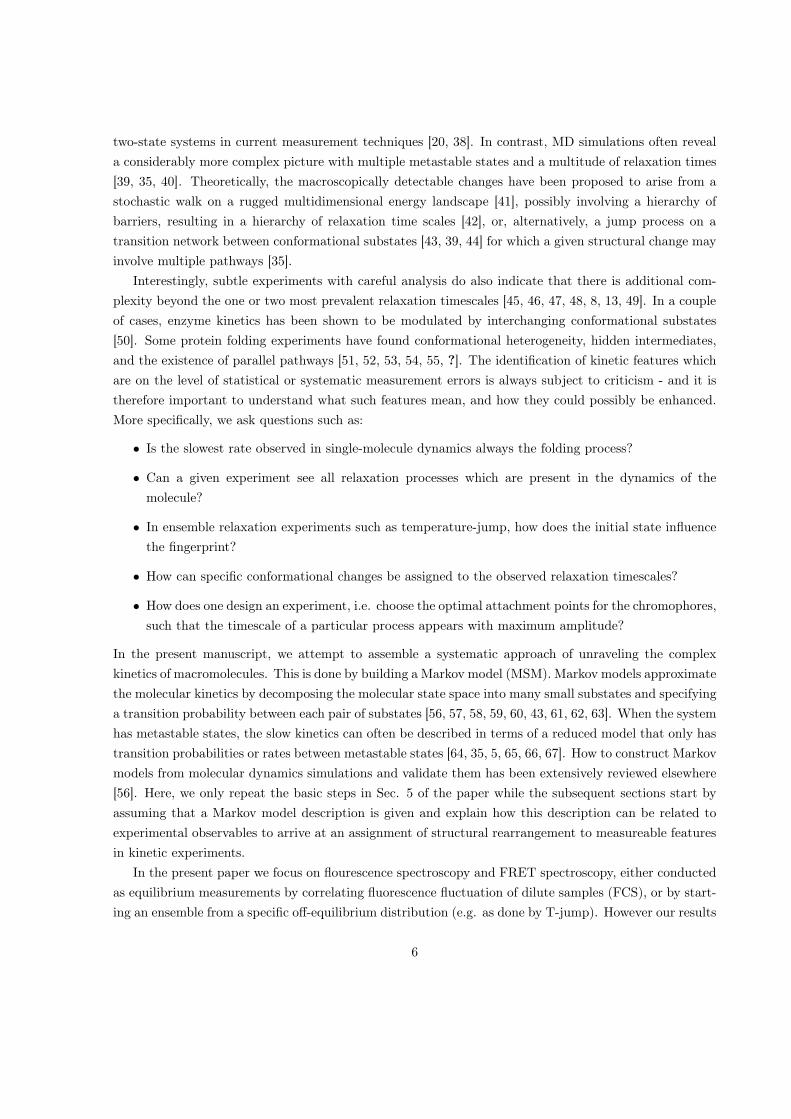
two-state systems in current measurement techniques [20, 38]. In contrast, MD simulations often reveala considerably more complex picture with multiple metastable states and a multitude of relaxation times[39, 35, 40]. Theoretically, the macroscopically detectable changes have been proposed to arise from astochastic walk on a rugged multidimensional energy landscape [41], possibly involving a hierarchy ofbarriers, resulting in a hierarchy of relaxation time scales [42], or, alternatively, a jump process on atransition network between conformational substates [43, 39, 44] for which a given structural change mayinvolve multiple pathways [35].

Interestingly, subtle experiments with careful analysis do also indicate that there is additional com-plexity beyond the one or two most prevalent relaxation timescales [45, 46, 47, 48, 8, 13, 49]. In a coupleof cases, enzyme kinetics has been shown to be modulated by interchanging conformational substates[50]. Some protein folding experiments have found conformational heterogeneity, hidden intermediates,and the existence of parallel pathways [51, 52, 53, 54, 55, ?]. The identification of kinetic features whichare on the level of statistical or systematic measurement errors is always subject to criticism - and it istherefore important to understand what such features mean, and how they could possibly be enhanced.More specifically, we ask questions such as:

• Is the slowest rate observed in single-molecule dynamics always the folding process?

• Can a given experiment see all relaxation processes which are present in the dynamics of themolecule?

• In ensemble relaxation experiments such as temperature-jump, how does the initial state influencethe fingerprint?

• How can specific conformational changes be assigned to the observed relaxation timescales?

• How does one design an experiment, i.e. choose the optimal attachment points for the chromophores,such that the timescale of a particular process appears with maximum amplitude?

In the present manuscript, we attempt to assemble a systematic approach of unraveling the complexkinet‌ics of macromolecules. This is done by building a Markov model (MSM). Markov models approximatethe molecular kinetics by decomposing the molecular state space into many small substates and specifyinga transition probability between each pair of substates [56, 57, 58, 59, 60, 43, 61, 62, 63]. When the systemhas metastable states, the slow kinetics can often be described in terms of a reduced model that only hastransition probabilities or rates between metastable states [64, 35, 5, 65, 66, 67]. How to construct Markovmodels from molecular dynamics simulations and validate them has been extensively reviewed elsewhere[56]. Here, we only repeat the basic steps in Sec. 5 of the paper while the subsequent sections start byassuming that a Markov model description is given and explain how this description can be related toexperimental observables to arrive at an assignment of structural rearrangement to measureable featuresin kinetic experiments.

In the present paper we focus on flourescence spectroscopy and FRET spectroscopy, either conductedas equilibrium measurements by correlating fluorescence fluctuation of dilute samples (FCS), or by start-ing an ensemble from a specific off-equilibrium distribution (e.g. as done by T-jump). However our results

6

are generally valid and an can be applied to any single-molecule experiment including AFM-pulling ex-periments.

7

2 Model of a protein folding equilibrium

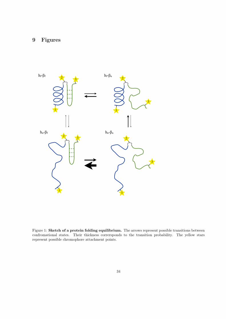
Consider the folding equilibrium of an illustrative protein folding model shown in fig. 1. The proteinconsists of two domains, an α-helix and a β-sheet, linked by a short loop regions. Each of the twodomains is assumed to fold and unfold independently of the other, which leads to a folding equilibriumwith four possible conformational states: (i) both domains folded hf -βf , (ii) helix folded and β-sheetunfdolded hf -βu, (iii) helix unfolded and β-sheet folded hu-βf , and (iv) both domains unfolded hu-βu.The transition between two of these states is called a conformational change, and the correspondingtransition probability is indicated by the thickness of the arrow between the two states.

We model the transitions between the conformations as a Markov jump process. While these modelstypically are a simplification of the true dynamics in the high-dimensional conformational space of themolecule, one often finds in practice that they constitute quantitatively correct and useful approximationsthat now have a solid theoretical foundation [68]. The Markov state model (MSM) directly yields therates of the dynamic processes which are present in the folding equilibrium. The rates which are measuredin experiments are associated to these processes. Note that, in most cases, they are not directly linkedto the transition rates between individual conformational states.

The model protein has three possible attachment sites for chromophores, represented by yellow starsnumbered 1 to 3 in fig. 1. In a classical single-molecule fluorescence quenching or FRET experiment, onewould chose two of these attachment points and measure the conformational dynamics as a projectiononto a coordinates that depends mainly on the distance between the two chromophores. By autocorre-lating the measured signal one can extract the timescales of the dynamics. However, which timescalesare observed not only depends on the underlying conformational equilibrium but also on the choice ofchromophore attachment points. When considering a temperature jump experiment of the same system,matters become even more complex, because now the observability of the system’s relaxation timescalesadditionally depends on the initial and final probability distribution of the system.

In section 3 we review how the measured spectrum emerges from the underlying MSM, the chosenobservable and the initial distribution. In section 4.2 we apply this theory to the model protein.

8

3 Theory

3.1 Markov state models

Consider a state space Ω consisting of N discrete microstates

Ω = S1, S2, ....SN .

In the context of molecules, this state space usually is the conformational space spanned by either all orthe most important conformational degrees of freedom of the molecule. A microstate is a small volumeelement in this high-dimensional space. The microstates cover the entire (accessible) space, but do notoverlap. See [56] for a discussion how this discretization of the continuous state space affects the qualityof the Markov model.

The movement of the molecule in this (conformational) state space is modeled as time-discrete processst with a time step τ

st = (s0, sτ , s2τ , s3τ ...) . (1)

The probability of finding the molecule in an state j at time t = nτ , in principle, depends on the entirehistory of the process

P(snτ = Sj | s(n−1)τ , s(n−2)τ , s(n−3)τ , ... s0).

Only if this long conditional probability can be truncated to

P(snτ = Sj | s(n−1)τ ),

the process is called Markovian [69]. The probability of finding the molecule in state j at time t = nτ

then only depends on the state the molecule has been in at the previous time step (memory-free process).These probabilities do not change in the course of the process (time invariant). They only depend on thepair of microstates snτ = Sj,s(n−1)τ = Si and the time step τ of the process. Arranged in a N × N

matrix, they form the transition matrix T(τ) with

Tij = P(snτ = Sj | s(n−1)τ = Si) ,

the central property of a Markov state model. The matrix elements represent the probability that themolecule is found in microstate Sj provided that it has been in microstate Si a time τ earlier. The ithrow of this transition matrix represents all possibilities a molecule in state i has: it can either stay in itscurrent microstate (Tii) or move to any of the other n− 1 microstates (Tij). Consequently, the elementsof each row in T(τ) sum up to 1

n

j=1

Tij = 1 , ∀i

(row-stochastic matrix).

9

Representing the conformational dynamics as a Markov state model is a good approximation if

1. the degrees of freedom (d.o.f.), which are not included in the model, (marginal d.o.f. or bath d.o.f.)move on faster time-scales than the d.o.f. included in the model (relevant d.o.f.) and are not coupledstrongly to the latter [63]

2. the conformational states of the molecule are projected onto disjunct regions in the space of therelevant d.o.f., i.e. they do not overlap

3. the transition region is sufficiently finely discretized [68, 70, 56], and

• the time step τ is large enough [68, 56].

While these requirements now have a solid theoretical underpinning, a practical analysis must test whetherthe MSM is consistent with the available simulation data within statistical errors [56]

The experiments we consider in the following, are conducted under equilibrium conditions. Hence,the dynamics can be represented by a single (time-invariant) transition matrix. Given a “good” Markovstate model, its transition matrix can be used to generate possible coarse-grained trajectories of a singlemolecule in the state space of the model. More importantly, the transition matrix contains the completeinformation of dynamics of an ensemble of molecules in this state space. Let p(t) be a probability vectorwith N elements, where the ith element represents the fraction of molecules in the ensemble which arefound in state Si at a time t. Consequently,

N

i=1

pi(t) = 1 .

The time evolution of this vector is completly determined by the transition matrix T(τ)

p(t+ τ) = p(t)T(τ) , (2)

where p(t) denotes the transpose of the vector p(t). Given an initial probility vector p(0), the probabilityat any discrete time kτ can be calculated by repeatedly applying T(τ) to it

p(kτ) = p(0)Tk(τ) = p(0)T(kτ). (3)

Eq. 2 and eq. 3 are equivalent, which becomes obvious if one realizes that p(2τ) = p(τ)T(τ) =

p(0)T(τ)T(τ) = p(0)T2(τ). They are known as the Chapman-Kolmogorov equation.If the potential energy surface on Ω is time invariant, then from physical intuition it is obvious that

there must be a stationary distribution π, and that this distribution may not change under the action ofT(τ), i.e.

πT = πTT(τ) (4)

10

Indeed, this stationary distribution emerges as the first left eigenvector of T(τ) associated with theeigenvalue λ1 = 1 [71]. Under equilibrium conditions, the dynamics of a molecular systems always fulfillsdetailed balance

πiTij = πjTji (5)

with respect to this stationary distribution π. This means that the number of systems in the ensemble,which go from state i to state j, is the same as the number of systems going from state j to i. This hasa number of convenient consquences on the properties of the MSM, as will be explained below.

Likewise, physical intuition tells us that any initial vector p(0) eventually converges to the stationarydistribution π. Indeed, one can show that for any p(0)

limk→∞

p(0)Tk(τ) = πT ,

where π is the first left eigenvector of T(τ).The transition matrix is, however, considerably more than a black box which converts the probability

at some point in time t to the probability at some time kτ later. The way the probability vector changeswith time and eventually converges to the stationary probability vector can be understood in terms ofthe eigenvectors of the transition matrix. This is illustrated in Fig. 2 (adapted from [56]) for a simpleexample.

The upper part in Fig. 2a shows a energy landscape along a single degree of freedom with fourenergy minina (A, B, C, D) and a high energy barrier between minima the two minima on the left sideof the coordinate (A, B) and those on the right (C, D). The coordinate is discretized into one hundredmicrostates. The lower part of Fig. 2a shows the corresponding equilibrium probability vector π at agiven temperature T . In Fig. 2b a transition matrix, which is given by a diffusion process on this energylandscape (see [56] for details), is presented. The matrix elements are color-coded: red represents hightransition probabilities between two microstates, and white or light blue represents transition probabilitieswhich are zero or close to zero. Reading the ith row from left to right, one finds the transition probabilitiesof from state xi into states which belong to minimum A (1 ≤ j < 25), to minimum B (25 ≤ j < 50),to minimum C (50 ≤ j < 75), and eventually to minimum D (75 ≤ j < 100). The four blocks alongthe diagonal structure of T(τ) correspond to the four minima in the energy surface. They reflect thefact that transitions within a minimum are much more likely than transitions from one minimum to theother.

These properties can be used in order to identify the metastable states of the system. The mathe-matical foundation for this was worked out in [59] and further developed in [65]. Metastability analysishas been subject to various studies and applications [5, 72, 35, 73] and is now a major tool to reduce thecomplexity of macromolecular kinetics to humanly understandable terms.

Transition matrices can, as any diagonalizable matrix, be written as a linear combination of their lefteigenvectors, their eigenvalues and their right eigenvectors

11

T(τ) =n

i=1

λi(τ)rili . (6)

and thus, for longer timescales:

Tk(τ) =n

i=1

λki (τ)ril

i . (7)

The transition matrix T(kτ) = Tk(τ) which transports an initial probability k time steps forward isagain a linear combination of the eigenvectors and eigenvalues. These linear combinations (eq. 6 and 7)are known as spectral decomposition of the transition matrix. They are very useful for connecting thedynamics of the molecule to the measured signal, which is in section 3.2.

Eq. 7 is the key for understanding how the transition matrix transforms a probability vector. Thecomplete process consists of n subprocesses rili , each of which is weighted by the eigenvalue λi raisedto the power k. Because the transition matrix is a row-stochastic matrix, it always has one eigenvaluewhich is equal to one λ1 = 1 [71]. Raising this eigenvalue to the power k does not change the weight ofthe corresponding subprocess r1l1 : 1k = 1. r1l1 is the stationary process, which we postulated in eq. 4,and l1 = π.

All other eigenvalues of the transition matrix are guaranteed to be smaller than one in absolute value[71]

|λi| ≤ 1 ∀i .

The weights of the corresponding processes, hence, decay exponentially

λki = exp (k lnλi) = exp

t

τlnλi

= exp

− t

ti

(8)

with the implied timescale ti of the decay process

ti = − τ

lnλi. (9)

The smaller the eigenvalue λi, the smaller the implied timescale ti, the faster the corresponding processdecays. Fig. 2d shows the 15 largest eigenvalues of the transition matrix in Fig. 2b. There is oneeigenvalue, λ1, which is equal to one, followed by three eigenvalues, λ2 to λ4, which are close to one. Thesefour dominant eigenvalues are separated by a gap from the remaining eigenvalues. Hence, the transitionmatrix consists of a stationary process, three slow processes and 96 processes which decay quickly. Aftera few time steps, only the four dominant processes contribute to the evolution of the probability vector.How these processes alter this vector, is determined by the shape of the corresponding eigenvectors.

Fig. 2c shows the four dominant right eigenvectors. The first eigenvector corresponds to the stationary

12

process and is, therefore, constant. The second eigenvector corresponds to the slowest process and haspositive signs in regions A and B and negative signs in regions C and D. This shape effectively movesprobability density across the largest barrier in the energy surface. Since the eigenvector is approximatelyconstant within the combined region (A,B) and (C,D) left and right of the barrier, it does not alter therelative probability distribution within these regions. The third eigenvector, analogously, moves densitybetween A and B, the fourth moves density between C and D.

A transition matrix which fulfills detailed balance (eq. 5) has several convenient properties. First, allof its eigenvalues and eigenvectors are guaranteed to be real. Second, defining a diagonal matrix Π inwhich the diagonal elements are equal to the equilibrium distribution π

Π : Πij =

πi if i = j

0 else,

the left and right eigenvectors are interconvertable [71]

li = Πri (10)

ri = Π−1li.

Hence, its spectral decomposition (eq. 7) can be written only in terms of the left eigenvectors

Tk(τ) = Π−1n

i=1

λki (τ)lil

Ti . (11)

In the experiments, which we discussed in the following sections, the dynamics of the molecule is governedby equilibrium dynamics (no varying forces, temperatures etc.). We will, therefore, always assume detailedbalance.

3.2 Calculating experimental expectation values from Markov models

We now consider the case that an experiment is conducted which measures observable a (and possiblyadditional observables b, c, ...). This observable has a scalar value for every state Si, although vector-or function-valued observables could be treated in a similar way. It is implicitly assumed that the statespace discretization used in the MSM in fine enough such that the value of a varies little within individualstates Si. The discretized observable vector a contains the mean values of individual states, ai.

We consider three different types of experiments: equilibrium experiments, relaxation experimentsand correlation experiments. In equilibrium experiments, the observed molecule is in equilibrium withthe current conditions of the surroundings (temperature, applied forces, salt concentration etc.), and themean value of an observable a, Eπ[a], is recorded. This may be either done my measuring Eπ[a] directlyfrom an unperturbed ensemble of molecules, or by recording sufficiently many and long single molecule

13

traces a(t) and averaging over them. The expression for the expected measured value of a is purelystationary, i.e., it does not depend on the time t:

Eπ[a] =N

i=1

aiπi = a, π . (12)

x, y denotes the Euclidean scalar product between two vectors x and y and E[...] the expectation value.In the second type of experiments, relaxation experiments, the observed molecule or ensemble is

allowed to equilibrate under a given set of conditions to the distribution p(0). At time t = 0 theseconditions are changed virtually instantaneously to another set of conditions which are associated witha different equilibrium distribution π. Now an observable a is traced over time whose mean value decaysfrom the old expectation Ep(0)[a] to the new expectation Eπ[a]. The way this relaxation, E[a(t)], hap-pens in time, allows conclusions on the intrinsic dynamical processes of the molecule. This principle isused in temperature- and pressure jump experiments. It can likewise be reproduced by single moleculeexperiments by measuring many trajectories whose conditions are rapidly changed at certain points intime, and then averaging over this trajectory ensemble. Single-molecule relaxation measurements can berealized e.g. by cycling the Mg2+ concentration in single-molecule FRET experiments or by changing thereference positions in optical tweezer experiments. Computationally, the dynamics of the molecule aftert = 0 are governed by a transition matrix T(τ) which reflects the conditions after the jump. At each timet = kτ , the ensemble will be distributed as pT (kτ) = pT (0)Tk(τ). The expectation value of a(t) changesaccordingly with time:

Ep(0)[a(kτ)] =N

i=1

aipi(kτ) = a,p(kτ). (13)

Using eq. 3, and eq. 11 one can expand eq. 13 to

E[a(kτ)] =a,

p(0)Tk(τ)

(14)

=

a,

p(0)Π−1

N

i=1

λki (τ)lil

i

=

a,

p(0)

N

i=1

λki (τ)lil

i

where we have replaced the probability distribution p(0) by the excess probability distribution

p(0) = Π−1p(0) (15)

14

with p

i(0) = pi(0)/πi. Rearranging the sum and the scalar products, one obtains

E[a(kτ ] =

a,

N

i=1

λki (τ)

p

(0), lili

(16)

=N

i=1

λki (τ)

a,

p

(0), lili

=N

i=1

λki (τ) a, li

p

(0), li

= a, πp

(0), π+

N

i=2

exp

− τ

ti

a, li

p

(0), li. (17)

The expected measured signal shows a multiexponential decay

f(t) = γ1 +

i=2

γrelaxi exp

− t

ti

, (18)

where γi is the amplitude of the a ith decay process and is given as

γrelaxi = a, li

p

(0), li

. (19)

The respective decay constant ti is equal to the ith implied timescale of the underlying transition matrix.Note that the individual components of the signal decay until the expected measured signal of theequilibrium experiment under the target conditions is reached

limk→∞

E[a(kτ)] = a, πp

(0), π= a, π = Eπ[a] .

The amplitudes γrelaxi in Eq. (eq. 19) reflect the extent to which a given mode (eigenvector) of the

dynamics influences the time-evolution of a(kτ)p(0). This depends on two factors

1. how much probability density is transported via this mode during the relaxation from p(0) to π,represented by the scalar product

p(0), li

2. how sensitive a is to changes along this mode, represented by the scalar product, a, li.

A third type experiments considered here are correlation experiments which report on the intrinsic molec-ular kinetics via time correlation functions of certain observables. One way to measure such correlationfunctions is by tracing the equilibrium fluctuations of a molecule subsequently correlating this signalin time. This is e.g. done in fluorescence correlation spectrosopy (FCS). In experiments, in which twosignals, a and b, are measured simultaneously, also cross-corrleation functions can be extracted from themeasured signal Multiparameter-FRET experiments [74, 75] or Multichromophore FRET experiments[7] are examples of this type of experiment. A way of directly measuring time correlation functions ofatomic positions are X-ray and neutron scattering experiments.

15

3.3 Calculating experimental correlation functions from Markov models

We now use the existing formalism to derive expressions which predict the auto-correlation functionof observable a and the cross-correlation function of observable a and b. Altough, to the best of ourknowledge, the auto- or crosscorrelation analysis of the measured signal has not been applied to relax-ation experiments yet, we also include this possibility into our derivation for completeness. In total, weobtain four different expressions for the four possible experimental situations (equilibrium or relaxationexperiment combined with either auto- or cross-correlation function). The respective expressions fo theamplitudes are summarized in Tab. 8.

We start with the most complex case: cross-correlation function in a relaxation experiment. All otherresults are specializations of this case. The movement of the molecule is represented by the jump processon the discrete microstates Si (eq. 1). Each state is associated with a value of each of the measured signal,represented by the signal vectors a and b. The correlation of a(t) and b(t), given an initial probabilityrepresented by p(0), is defined as

Ep(0)[cor(a, b; τ)] =N

i=1

N

j=1

aiP(s0 = Si) · bjP(skτ = Sj | s0 = Si)

=N

i=1

N

j=1

aipi(0) · bjP(skτ = Sj | s0 = Si)

If st is a Markov processes with transition matrix T(τ), then the conditional probability P(skτ = Sj |s0 = Si) can be replaced by the corresponding matrix element

Tk(τ)

ij

of the transition matrix raised tothe power k. Introducing a diagonal matrix P(0) in which the diagonal elements are equal to the initialprobability vector Pii(0) = pi(0) , we can formulate the cross-correlation function as a vector-matrixequation

Ep(0)[cor(a, b; kτ)] = aP(0)Tk(τ)b. (20)

We introduce an excess initial density P(0) = Π−1P(0) (analogous to eq. 15), replace the transitionmatrix by its spectral decomposition (eq. 11), use the definition of the implied timescale (eq. 8) andobtain an expression which has the same structure as eq. 18

16

Ep(0)[cor(a, b; kτ)] = aTP(0)Π−1

N

i=1

λki lil

i

b

=N

i=1

λki

N

r,s=1

arpr(0)

πr

lil

i

rsbs

=N

i=1

λki

N

r,s=1

arpr(0)

πrlis lis bs

=N

i=1

λki a,P(0)li b, li

= a,P(0)π b,π+N

i=2

exp

−kτ

ti

a,P(0)li b, li (21)

The ith decay constant of this multiexponential decay is given as the implied timescale associated withthe ith eigenvector of the transition matrix. The corresponding amplitude is given as

γrelax, cross-cori = a,P(0)li b, li . (22)

The autocorrelation function of a relaxation experiment is obtained by replacing the signal vector b bya in eq. 20 and 21

Ep(0)[cor(a, a; kτ)] = a,p(0) a,π+N

i=1

exp

−kτ

ti

a,P(0)li a, li .

with the amplitudes

γrelax, auto-cori = a,P(0)li

2. (23)

In the more common case that the correlation functions are measured under equilibrium conditions,the initial density equals the equilibrium density and consequently P(0) is equal to the identity matrix.The cross- and autocorrelation are thus given as

Eπ[cor(a, b; kτ)] =N

i=1

λki a, li b, li

= a,π b,π+N

i=2

exp

−kτ

ti

a, li b, li

with the amplitudes

17

γcross-cori = a, li b, li . (24)

and

Eπ[cor(a, a; kτ)] =N

i=1

λki a, li

2

= a,π2 +N

i=2

exp

−kτ

ti

a, li2 . (25)

with the amplitudes

γcross-cori = a, li2 . (26)

18

4 Application to model systems

4.1 1D energy surface

Figure 3 shows the eigenvectors of our model of an one-dimensional energy surface (fig. 2), two differentobservables and two different initial distributions. The observables model a fluorescence quenching ex-periment. With a1 the chromophore fluoresces if the system is in state A or B, whereas fluorescence isquenched in state C and D. With a2 fluorescence is quenched in A, B, and D.

Due to the hierachical nature of the energy landscape an interpretation of the measured timescalesin terms of individual conformational changes can be misleading. In a four state system, there are sixpossible transitions, i.e. six possible conformational changes. Yet the dynamics in this state space isdescribed by only three relaxation processes (non-stationary eigenvectors of the corresponding transitionmatrix). Processes three and four indeed correspond mostly to transitions from one conformational stateto another. However, process two represents the transition between the group A,B and the groupC,D, i.e. it can be associated to the transition across the barrier separating B and C.

The stationary process is always detected. The overlap between the observables and the initial dis-tributions with the eigenvectors of the model, represented by the respective scalar product, are shown tothe left and right of the eigenvector plots in Fig. 3. Because the stationary distribution l1 = π has onlypositive entries, the scalar product with any observable or any initial distribution is greater than zero.Consequently, γ1 in eq. 18 is always greater than zero. Although dynamical fingerprints do normally notinclude this stationary part [73], we here include the overlap of observable and initial distributions withthe stationary process for completeness.

Not all dynamical processes can be detected. Whether a given process appears in the experimentalfingerprint depends on the overlap of the observable with this process. For example, the overlap of a1with the third and the fourth process is nearly zero. These processes correspond to swaps between stateswhich have the same signal value (A ↔ B and C ↔ D). Hence, a2 is insensitve to them, and γ3 ≈ 0, andγ4 ≈ 0 in an autocorrelation experiment (eq. 25). Only the second process can be observed with a1. a2

is sensitive to the second and fourth process but not to the third. Compare the scalar products in Fig.3 with the Fig. 4a and 4b.

By a clever choice of a and p(0) one can selectively measure a specific process. It is not possibleto observer processes in a relaxation experiment which would be invisible in an equilibrium experiment(Fig. 4c and 4d), because the amplitude is proportional to the overlap of the observable with theeigenvector (Eq. 23). The amplitude is also proportional to the overlap of the eigenvector with the initialdistribution. By choosing the initial distribition appropriately one can “hide” processes which are visiblein the equilibrium experiment. This allows for the selective measurement of processes which might behard to extract from the multiexponential decay in the corresponding equilibrium experiment, for exampleprocesses which decay on short timescales. This is shown in Fig. 4f. An unwise combination of observableand initial distribution, however, may lead to a spectrum in which only the stationary process can beobserved (Fig. 4e).

19

4.2 Protein folding model

We model the folding equilibrium of the model protein (Fig. 1) as a Markov model with four states whichare defined as: state 1 = hfβf (both domains folded), state 2 = hfβu (helix folded, β-sheet unfolded),state 3= huβf (helix unfolded, β-sheet folded), state 4 = huβu (both domains unfolded). Suppose, wehave observed the protein and took note of the transitions after each time step τ . The matrix

C(τ) =

12000 20 2 0

20 7000 0 2

2 0 6000 20

0 2 20 1000

. (27)

contains the total number of observed transitions. By normalizing each row one obtains the correspondingtransition matrix

T (τ) ≈

0.9982 0.0017 0.0002 0

0.0028 0.9969 0 0.0003

0.0003 0 0.9963 0.0033

0 0.0020 0.0196 0.9785

(28)

which represents the Markov model. Note that due to rounding errors, the rows in eq. 28 do not exactlysum up to one.

The thickness of the arrows in Fig. 1 reflect the transition probabilities between the states. There is afast equilibrium between the folded and the unfolded conformation of the β-sheet if the helix is unfolded.The folding of the complete protein mainly occurs through a cooperative folding pathway via the statehfβu . Folding of the helix when the β-sheet is already formed is considerably less likely. The eigenvaluespectrum, as well as the left and right eigenvectors of T are shown in Fig. 5.

The slowest rate in the system is not a priori the “folding rate” of the protein. The timescales observedin single-molecule experiments are often interpreted in terms of conformational changes in the examinedmolecule, and the slowest process is typically associated with the overall folding and unfolding. In thepresent example, the folding rate could either be defined as the rate of going from state 4 to state 1, oras the rate of going from the ensemble of states 2, 3, and 4 to state 1. However, none of the eigenvectorscorresponds to either of the two processes. Rather they have the following interpretation: l2 representsthe folding and unfolding of the helix, l3 represents the folding equilibrium of the β-sheet when the helixis already formed, and l4 represents the same equilibrium when the helix is unfolded. Care should betaken to differentiate between the folding rate and the rate limiting step in a folding equilibrium whichin this case is the formation of the helix.

Fig. 5b shows two initial distributions, as they could be used in jump experiments. The first one(p1(0)) represents an ensemble in which all systems are folded, the second one (p2(0)) an ensemble inwhich all systems are completely unfolded. Fig. 5c shows observable vectors which correspond to aFRET experiment in which the chromophores are attached at sites 1 and 2 (a1), sites 2 and 3 (a2), and

20

sites 1 and 3 (a3). For all three observables, we discuss the autocorrelation fingerprints of equilibriumexperiments. We also discuss an equilibrium multichromophore experiment in which observables a1 anda2 are combined (donor at site 2, first acceptor at site 1, second acceptor at site 3). As for the relaxationexperiments, we discuss the combination of the two initial distributions with observable a3.

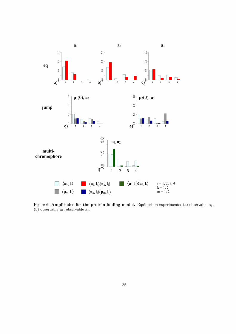
The three observables are an intuitive example why some observables do not resolve all processespresent in the system. From Fig. 1 it is clear that, if the chromophores are attached at site 1 and 2(observable a1), the experiment will only be sensitive to processes which involve the folding or unfoldingof the helix. This is reflected in the scalar products of a1 with the l2, l3, and l4 (table 6). a1 has a largeoverlap with l2, but only small or virtually no overlap with l4, and l3. Correspondingly, a2 (chromophoresattached at sites 2 and 3) is sensitive to l3, and l4, which represent the folding of the β-sheet, but ratherinsensitive to l2. a3 (chromophores attached to sites 1 and 3) is sensitive to all three processes. Theexpected amplitudes of equilibrium experiments with a1, a2, or a3 are shown in Fig. 6a-c.

Given only the three-dimensional structure of a molecule it is often impossible to decide whether aparticular observable can resolve all processes in the conformational equilibrium. However, with the helpof MD simulations one can quantify the sensitivity of the observable to any process in the equilibrium.This is discussed in section 5.

The two initial probability distributions illustrate a pitfall of jump experiments. Not all processesare used when the system relaxes from a particular initial distribution to the equilibrium distribution.For example, in the relaxation from the folded state (p1(0)) the equilibrium between the folded and theunfolded conformation of the β-sheet is entirely achieved via l3, and not via l4 (table 2: p1(0), l3 =0.50,p1(0), l4 =0.00). When the system is relaxed from the unfolded state (p2(0)), however, the situationis reversed: l4 is active, wheras l3 is not (table 2: p2(0), l3 =0.06, p2(0), l4 =1.09). Therefore, evenwhen an observable which is sensitive to all processes is chosen, like a3 in the present example, someprocesses might still be undetectable in a relaxation experiment. Fig. 6d and 6e. shows the expectedamplitudes for the two relaxation experiments. For p1(0) the fourth process has no amplitude, and forp2(0) the third process has a very small amplitdue.

With multichromophore experiments the trade-off between selectivity and comprehensiveness is alle-viated. An observable like a3 has the advantage of comprehensiveness. However, it can be very tediousand difficult to extract multiple timescales from a possibly noisy data set. In principle, it would possibleto perform several experiment on a given system, each with a different observable, and combine theobtained results. Unless the sensitivity of the observables to the processes in the system is known, it willbe hard to decide whether peaks which appear with similar timescales in two different experiments arethe same conformational process slightly shifted or two different conformational processes with similartimescales. By performing a multiple-chromophore experiment one obtains the information of the twoindividual experiments, and additionally can use the information from the cross-correlation from the twosignals to match peaks from the individual experiments (Fig. 6f) If two peaks in the individual experi-ments correspond to the same conformational process i, the amplitude in the cross-correlation fingerprintshould be a1, lia2, li, where a1, li and a2, li are obtained as the square-root of the amplitudes inthe respective auto-correlation fingerprint. If, on the other hand, the two individual experiments measure

21

disjunct sets of processes (as in our example), the amplitudes of in the cross-correlation fingerprint shouldbe close to zero.

22

5 Experimental design using MD and MSM

5.1 Experimental dynamical fingerprints

To reconcile our Markov model analysis with measured data, it is useful to transform the experimentalrelaxation curve into timescales and amplitudes. In practice, this is often done by fitting a single- ormultiexponential model. This approach is not objective as it requires the number of timescales to befixed. For example, multiple exponentials with similar timescales, or a double-exponential where thelarger timescale has a small amplitude will both yield visually excellent single-exponential fits with aneffective timescale that may not exist in the underlying system (see [39] and SI of [73]). To preparethe experimental data for a systematic analysis, we propose to use a method that uniquely transformsthe observed relaxation profile into an amplitude density of relaxation timescales (here called dynamicalfingerprints). Several such methods have been developed especially maximum entropy or least squaresbased methods [76, 77]. In [73] we have developed a maximum-likelihood method which is availablethrough the package SCIMEX (e.g. https://simtk.org/home/scimex) which is briefly discussed here.

Suppose a correlation or relaxation function xj = x(tj) is given (e.g. from an experiment) at real timepoints t1, ..., to. We expect from physical principles that this signal is a noisy realization of a functionthat is in fact a sum of multiple exponentials with initially unknown timescales and amplitudes, i.e. afunction that can be represented by

yΦ(t) =

ˆtdt γ(t) exp

− t

t

,

i.e. the Laplace transform of the amplitude spectrum, or “fingerprint”, γ(t) is expected to consist ofpeaks. To computationally determine this fingerprint the timescale axis t needs to be discretized usingn spectral time points t1, ..., t

n. With a fine timescale discretization we obtain a good approximation of

the fingerprint:

yΦ(t) ≈n

i=1

ai exp

− t

t

.

where the amplitudes ai define a set of parameters Φ = ai = a(ti) defining the fingerprint thatneeds to be determined. When each observation xj comes with a Gaussian-shaped uncertainty σj , thelog-Likelihood of a given fingerprint having generated the observed signal x is given by (up to an irrelevantadditive constant):

log p(x|Φ) =o

j=1

(xj −n

i=1 ai exp(−tj/ti))2

2σ2j

(29)

And the amplitudes are estimated as the maximum of this function, yielding the discretized maximum-likelihood fingerprint [(t1, a1), ..., (t

n, an)]. As an example, we consider a hypothetical measurement of a

23

correlation function of the form

y(t) = 0.9 exp

t

50

+ 0.1 exp

t

250

(30)

with additive Gaussian error having intensities of σ = 0.5/√t. Fig. 7c shows the curve of Eq. (30)

along with the measured correlation function, while Fig 7a (black) shows the corresponding fingerprint.Figs 7a (red), b, and c(green) show the results of the fingerprint estimation procedure. The experimentalfingerprint shown in Figs 7a is then used for the further analysis.

5.2 Simulation, Markov model, and simulated dynamical fingerprints

Molecular simulation methods are useful to generate structures that can be assigned to experimentallymeasurable dynamical processes. A popular choice are atomistic molecular dynamics models, but in somecases higher-order models (such as ab initio or QM/MM) or coarser methods (coarse-grained modelsor Go-type models) may be useful. Furthermore, a simulation setup should be chosen which is ableto generate dynamical trajectories from some well-defined ensemble. At least, one expects a constanttemperature and a unique stationary density (see [56, 78] for a discussion on ensembles and thermostatsthat have desirable statistical properties). Based on such a setup, dynamical trajectories can be generated.At this point, we assume that the setup and the computational environment has been chosen such that a“statistically sufficient” amount of trajectories can be generated. In situations where this is not possible,see [35, 79, 80, 81, 82] for a discussion of methods that can be used to enhance the sampling.

Given the simulation data, the molecular state space is discretized by clustering. Various combina-tions of distance metrics and clustering methods have been proposed. Frequently used metrics includeEuclidean distance after having fitted the molecule to a reference structure [35, 5], root mean squaredistance (RMSD) [44, 58], and various clustering methods may be used [35, 44, 58, 72, 83]. Interestingly,very simple methods such as choosing generator structures by picking simulation frames at regular timeintervals or even randomly and then clustering the data by assigning all simulation frames to the nearestgenerator structures perform quite well [56]. Importantly, the clustering must be fine enough such thatthe discretization is still allows the metastable states to be distinguished in order to be useful to build aquantitative Markov model.

After having discretized the simulation data to discrete trajectories, the transition matrix T(τ) isestimated. The simplest method to do this is to generate a count matrix C(τ) whose entries cij containthe number of times a simulation was found in state i in time t and in j at time t + τ , and thencalculating Tij = cij/

k cik. However, this matrix does not necessarily fulfill detailed balance, and thus

the decomposition Eq. (7) does not have a simple interpretation. It is therefore desirable to estimatea matrix T(τ) that fulfills detailed balance. Reversible counting [39] can be used if one has simulationtrajectories that are much longer than the slowest relaxation time, otherwise one must use an estimationmethod [56] which allow a reversible T(τ) to be estimated based on the unbiased count matrix C(τ).

In order to analyze T(τ), we perform an eigenvalue decomposition, generating eigenvectors li andeigenvalues λi. The eigenvectors can be used to identify metastable sets [59, 65, 5] that help to understand

24

the essential kinetics. The eigenvectors li can be investigated in order to obtain insight between whichstates the relaxation process with timescale ti = −τ/ lnλi switches.

The fingerprint is calculated by calculating the amplitudes depending on the specific type of exper-iment considered (see Sec. 3.2 and 3.3) and combining them with the timescales ti. Note that thisfingerprint has statistical uncertainty based on the fact that only a finite number of dynamical trajec-tories has been used for the estimation of T(τ). This uncertainty can be characterized based on MonteCarlo methods described in [60, 84, 73].

The assignment of structural processes to experimentally-detected dynamical features can be made ifpeaks can be matched between

Programs to calculate Markov models from simulation data are available in the simulation packagepackage EMMA (e.g. https://simtk.org/home/emma)

5.3 Validation and experimental design

We have discussed and shown in Sec. 4 that for each given experimental setup (i.e. combination ofmeasurement technique and observable chosen by the label placement), the amplitude of some processesmay be large, and the amplitude of many others may be small. The small-amplitude processes can oftennot be detected with high reliability since they might affect the signal only to a degree that is similar tostatistical or systematic error present in the measurement. It is thus desirable to design the experimentsuch that specific processes appear with large amplitudes. We sketch the following systematic approachof experimental design which has been proposed in [73]:

1. Conduct MD simulations of the molecular system under investigation and estimate a Markov modelto model its essential kinetics

2. For each possible experimental setup (e.g. for each placement of the labels), estimate the valuesof the corresponding observables, a, b and calculate the expected experimental fingerprints asdescribed in Sec. 3.2 and 3.3.

3. For each of the m slowest relaxation processes, select the experimental setup for which the amplitudeof this relaxation process is largest (or largest compared to the amplitudes of the processes withsimilar timescales if the timescale spectrum is dense)

4. Conduct these m experiments.

This approach attempts to optimally probe each process with a single experiment, thus also keepingthe number of potentially expensive experiments small. Besides yielding a useful set of complementaryexperiments, this approach is useful to validate the simulated results much more solidly than with a singlecomparison.

This approach is ideally suited for experiments with site-specific labels that do not significantly affectthe kinetics. This is especially true for techniques that permit isotope labeling such as NMR, IR spec-troscopy or neutron scattering. In fluorescence-based techniques this can be achieved with intrinsic dyes

25

(e.g. the modulation of Tryptophan fluorescence by the environment [37] or Tryptophan triplet quenchingby Cysteine [85]) or with extrinsic dyes that have little effect on the conformational dynamics.

In [73], the method has been demonstrated on the MR121-GS9-W peptide with a simple heuristic topredict fluorescence signals for each of 190 possible positions of the MR121 and W dyes along the chain.Based on this, the amplitudes of the five slowest fingerprint peaks were calculated and are shown in Fig.9. It is apparent that for most experiments only one or two amplitudes are strong while the remainingamplitudes are weak. If this result is also true for other molecules, it is evident why so many moleculesappear to have two- or three-state kinetics while they are much more complex in molecular simulations.

Based on such a comparison of predicted fingerprints, experiments can be suggested. The coloredboxes in Fig. 9 highlight five experiments that are predicted to maximally probe each of the slowestrelaxation processes relative to the total amplitude of the five slowest processes.

26

6 Conclusions

The combination of Markov models and the concept of dynamical fingerprints provides a theoreticallysolid and computationally feasible approach to connect molecular simulation data or molecular kineticmodels to experiments that probe the kinetics of the molecular system in reality. The main advantageof this approach over traditional MD analyses is that the processes that occur at given timescales areunambiguously given by the theory. In the Markov model, this assignment is present by the one-to-oneassociation of transition matrix eigenvalues (that correspond to measurable relaxation timescales) andeigenvectors (that describe structural changes). When the experimentally-measured relaxation data isfurther subjected to a spectral analysis, experiment and simulation can be reconciled on the basis ofdynamical fingerprints, i.e. by matching peaks of the timescale density.

A comment is in order on the fact that in all cases, the slow relaxations in kinetic measurements arefound to have the form of a sum of single exponential term, each term corresponding to an eigenvalue/ eigenvector pair in our analysis. This is a general result which can also be obtained by performingthe analysis in full continuous state space (as opposed to our discrete-state treatment here). The onlyassumptions that are made to arrive at this result are the following:

1. The dynamics of the system is Markovian in full state space (i.e. the continuous space of allpositions and momenta of the molecular systems studied and the solvent molecules). This is avery weak assumption that is made in all classical simulation models. The Markovian assumptioncould also be applied to quantum mechanical models when the electronic degrees of freedom areincluded. It is thus also a reasonable assumption for real molecular systems. The only systems forwhich such an assumption would be unpractical are systems which have correlations over arbitrarilylong lengthscales, such that no finite-size simulation setup can be made that captures all relevantprocesses. This can happen for glassy or crystalline systems.

2. The state space is ergodic, i.e. all states of the system can interchange. This assumption may alsobe untrue for glassy or crystalline systems. It is in practice also hard to fulfill for other systemsif the kinetics are slow and are not measured in an ensemble but by averaging multiple single-molecule trajectories. In this case it may be difficult to collect sufficiently many trajectories thatthis trajectory set is effectively ergodic, and deviations from multiexponentiality may be a statisticalartefact.

3. The relaxations are measured at equilibrium conditions. This does include the possibility that thesystem relaxes from an off-equilibrium distribution (e.g. as in temperature jump experiments), butit does so under equilibrium dynamics which fulfill detailed balance. This assumption requires thatthe experiment does not put energy into the system or remove energy from it. It is unclear whetherlaser or scattering experiments obey this condition sufficiently well.

Even in situations where these points can be assumed to be fulfilled, apparent nonexponentiality has beenfound over significantly long timescales, such as stretched exponentials [86, 87] or power laws [47]. Notethat this is no contradiction because such apparent nonexponentialities can be easily explained by sums

27

of a few single exponential relaxations with particular spacings of timescales and amplitudes [88, 89, 73]- and thus also correspond to dynamical fingerprints with multiple peaks (see [73], Supplementary Fig. 1and 2). In practice, however, care must be taken that such effects are not actually due to the measurementtechnique itself. Especially conditions 2 and 3 may sometimes be violated by the experimental setup itself.

It is likely that the apparent two- or three-state kinetics observed in experiments of macromoleculesdoes not reflect the entire complexity of their conformational dynamics. In particular, the slowest mea-sured rate is not necessarily the folding rate because (i) there might be no process which corresponds toour notion of folding, (ii) the experiment might be insensitive to this particular process. The comparisonto a Markov model allows for a unambiguous interpretation of the measured fingerprints.

7 Acknowledgments

Funding from the German Science Foundation (DFG) through grant number NO 825/2 and throughresearch center MATHEON is gratefully acknowledged.

References

[1] S. Fischer, B. Windshuegel, D. Horak, K. C. Holmes and J. C. Smith. Proc. Natl. Acad. Sci. USA102 (2005), pp. 6873.

[2] P. Imhof, S. Fischer and J. C. Smith. Biochemistry 48 (2009), pp. 9061.

[3] A. H. Ratje, J. Loerke, A. Mikolajka, M. Brunner, P. W. Hildebrand, A. L. Starosta, A. Donhofer,S. R. Connell, P. Fucini, T. Mielke, P. C. Whitford, J. N. Onuchic, Y. Yu, K. Y. Sanbonmatsu, R. K.Hartmann, P. A. Penczek, D. N. Wilson and C. M. T. Spahn. Nature 468 (2010), pp. 713.

[4] J. Nguyen, M. A. Baldwin, F. E. Cohen and S. B. Prusiner. Biochemistry 34 (1995), pp. 4186.

[5] F. Noé, I. Horenko, C. Schütte and J. C. Smith. J. Chem. Phys. 126 (2007), p. 155102.

[6] B. Schuler, E. A. Lipman and W. A. Eaton. Nature 419 (2002), pp. 743.

[7] J. Ross, P. Buschkamp, D. Fetting, A. Donnermeyer, C. M. Roth and P. Tinnefeld. J. Phys. Chem.B 111 (2007), pp. 321.

[8] Y. Santoso, C. M. Joyce, O. Potapova, L. Le Reste, J. Hohlbein, J. P. Torella, N. D. F. Grindleyand A. N. Kapanidis. Proc. Natl. Acad. Sci. USA 107 (2010), pp. 715.

[9] A. Y. Kobitski, A. Nierth, M. Helm, A. Jäschke and G. U. Nienhaus. Nucleic Acids Res. 35 (2007),pp. 2047.

[10] W. J. Greenleaf, M. T. Woodside and S. M. Block. Annual review of biophysics and biomolecularstructure 36 (2007), pp. 171.

28

[11] J. Cellitti, R. Bernstein and S. Marqusee. Protein Science 16 (2007), pp. 852.

[12] M. Rief, M. Gautel, F. Oesterhelt, J. M. Fernandez and H. E. Gaub. Science 276 (1997), pp. 1109.

[13] Gebhardt, T. Bornschlögl and M. Rief. Proc. Natl. Acad. Sci. USA 107 (2010), pp. 2013.

[14] H. Wu and F. Noé. Phys. Rev. E, published online (2011).

[15] I. V. Gopich and A. Szabo. J. Phys. Chem. B 113 (2009), pp. 10965.

[16] H. Wu and F. Noé. Multiscale Model. Simul. 8 (2010), p. 1838.

[17] I. V. Gopich, D. Nettels, B. Schuler and A. Szabo. J. Chem. Phys. 131 (2009), p. 095102.

[18] M. Jäger, Y. Zhang, J. Bieschke, H. Nguyen, M. Dendle, M. E. Bowman, J. P. Noel, M. Gruebeleand J. W. Kelly. Proc. Natl. Acad. Sci. USA 103 (2006), pp. 10648.

[19] M. Sadqi, L. J. Lapidus and V. Munoz. Proc. Natl. Acad. Sci. USA 100 (2003), pp. 12117.

[20] C. Dumont, T. Emilsson and M. Gruebele. Nature Meth. 6 (2009), pp. 515.

[21] C.-K. Chan, Y. Hu, S. Takahashi, D. L. Rousseau, W. A. Eaton and J. Hofrichter. Proc. Natl. Acad.Sci. USA 94 (1997), pp. 1779.

[22] A. Volkmer. Biophys. J. 78 (2000), pp. 1589.

[23] I. Schlichting, S. C. Almo, G. Rapp, K. Wilson, K. Petratos, A. Lentfer, A. Wittinghofer, W. Kabsch,E. F. Pai, G. A. Petsko and R. S. Goody. Nature 345 (1990), pp. 309.

[24] J. Buck, B. Fürtig, J. Noeske, J. Wöhnert and H. Schwalbe. Proc. Natl. Acad. Sci. USA 104 (2007),pp. 15699.

[25] T. Kiefhaber. Proc. Nat. Acad. Sci. USA 92 (1995), pp. 9029.

[26] W. Doster, S. Cusack and W. Petry. Nature 337 (1989), pp. 754.

[27] L. J. Lapidus, W. A. Eaton and J. Hofrichter. Proc. Natl. Acad. Sci. USA 97 (2000), pp. 7220.

[28] H. Neuweiler, M. Löllmann, S. Doose and M. Sauer. J. Mol. Biol. 365 (2007), pp. 856.

[29] X. Michalet, S. Weiss and M. Jäger. Chem. Rev. 106 (2006), pp. 1785.

[30] P. Tinnefeld and M. Sauer. Angew. Chem. Intl. Ed. 44 (2005), pp. 2642.

[31] R. R. Hudgins, F. Huang, G. Gramlich and W. M. Nau. J. Am. Chem. Soc. 124 (2002), pp. 556.

[32] H. D. Kim, G. U. Nienhaus, T. Ha, J. W. Orr, J. R. Williamson and S. Chu. Procl. Natl. Acad. Sci.USA 99 (2002), pp. 4284.

[33] D. Nettels, A. Hoffmann and B. Schuler. J. Phys. Chem. B 112 (2008), pp. 6137.

29

[34] D. D. Schaeffer, A. Fersht and V. Daggett. Curr. Opin. Struct. Biol. 18 (2008), pp. 4.

[35] F. Noé, C. Schütte, E. Vanden-Eijnden, L. Reich and T. R. Weikl. Proc. Natl. Acad. Sci. USA 106(2009), pp. 19011.

[36] W. van Gunsteren, J. Dolenc and A. Mark. Curr. Opin. Struct. Biol. 18 (2008), pp. 149.

[37] M. Jäger, H. Nguyen, J. C. Crane, J. W. Kelly and M. Gruebele. J. Mol. Biol. 311 (2001), pp. 373.

[38] O. Bieri, J. Wirz, B. Hellrung, M. Schutkowski, M. Drewello and T. Kiefhaber. Proc. Natl. Acad.Sci. USA 96 (1999), pp. 9597.

[39] S. Muff and A. Caflisch. Proteins 70 (2007), pp. 1185.

[40] D. L. Ensign, P. M. Kasson and V. S. Pande. J. Mol. Biol. 374 (2007), pp. 806.

[41] J. N. Onuchic and P. G. Wolynes. Curr. Opin. Struc. Biol. 14 (2004), pp. 70.

[42] H. Frauenfelder, G. Chen, J. Berendzen, P. W. Fenimore, H. Jansson, B. H. McMahon, I. R. Stroe,J. Swenson and R. D. Young. Proc Natl. Acad. Sci. USA 106 (2009), pp. 5129.

[43] F. Noé and S. Fischer. Curr. Opin. Struc. Biol. 18 (2008), pp. 154.

[44] G. R. Bowman, K. A. Beauchamp, G. Boxer and V. S. Pande. J. Chem. Phys. 131 (2009), p. 124101.

[45] A. Gansen, A. Valeri, F. Hauger, S. Felekyan, S. Kalinin, K. Tóth, J. Langowski and C. A. M. Seidel.Proc. Natl. Acad. Sci. USA 106 (2009), pp. 15308.

[46] H. Neubauer, N. Gaiko, S. Berger, J. Schaffer, C. Eggeling, J. Tuma, L. Verdier, C. A. Seidel,C. Griesinger and A. Volkmer. J. Am. Chem. Soc. 129 (2007), pp. 12746.

[47] W. Min, G. Luo, B. J. Cherayil, S. C. Kou and X. S. Xie. Phys. Rev. Lett. 94 (2005), p. 198302.

[48] E. Z. Eisenmesser, O. Millet, W. Labeikovsky, D. M. Korzhnev, M. Wolf-Watz, D. A. Bosco, J. J.Skalicky, L. E. Kay and D. Kern. Nature 438 (2005), pp. 117.

[49] B. G. Wensley, S. Batey, F. A. C. Bone, Z. M. Chan, N. R. Tumelty, A. Steward, L. G. Kwa,A. Borgia and J. Clarke. Nature 463 (2010), pp. 685.

[50] B. P. English, W. Min, A. M. van Oijen, K. T. Lee, G. B. Luo, H. Y. Sun, B. J. Cherayil, S. C. Kouand X. S. Xie. Nature Chemical Biology 2 (2006), pp. 87.

[51] M. O. Lindberg and M. Oliveberg. Curr. Opin. Struct. Biol. 17 (2007), pp. 21.

[52] K. Sridevi. J. Mol. Biol. 302 (2000), pp. 479.

[53] R. A. Goldbeck, Y. G. Thomas, E. Chen, R. M. Esquerra and D. S. Kliger. Proc. Natl. Acad. Sci.USA 96 (1999), pp. 2782.

30

[54] A. Matagne, S. E. Radford and C. M. Dobson. J. Mol. Biol. 267 (1997), pp. 1068.

[55] C. C. Mello and D. Barrick. Proc. Natl. Acad. Sci. USA 101 (2004), pp. 14102.

[56] J.-H. Prinz, H. Wu, M. Sarich, B. Keller, M. Fischbach, M. Held, J. Chodera, C. Schütte and F. Noé.J. Chem. Phys. (2011).

[57] W. C. Swope, J. W. Pitera, F. Suits, M. Pitman and M. Eleftheriou. J. Phys. Chem. B 108 (2004),pp. 6582.

[58] J. D. Chodera, K. A. Dill, N. Singhal, V. S. Pande, W. C. Swope and J. W. Pitera. J. Chem. Phys.126 (2007), p. 155101.

[59] C. Schütte, A. Fischer, W. Huisinga and P. Deuflhard. J. Comput. Phys. 151 (1999), pp. 146.

[60] F. Noé. J. Chem. Phys. 128 (2008), p. 244103.

[61] V. S. Pande, K. Beauchamp and G. R. Bowman. Methods 52 (2010), pp. 99.

[62] N. V. Buchete and G. Hummer. J. Phys. Chem. B 112 (2008), pp. 6057.

[63] B. Keller, P. Hünenberger and W. van Gunsteren. J. Chem. Theo. Comput., published online (2011).

[64] S. Kube and M. Weber. J. Chem. Phys. 126 (2007), p. 024103.

[65] M. Weber. ZIB Report 03-04 (2003).

[66] C. Schütte, F. Noé, E. Meerbach, P. Metzner and C. Hartmann. In R. Jeltsch and G. W. (Eds), eds.,Proceedings of the International Congress on Industrial and Applied Mathematics (ICIAM). EMSpublishing house, pp. 297–336.

[67] C. Schütte and W. Huisinga. In P. G. Ciaret and J. L. Lions, eds., Handbook of Numerical Analysis,volume X: Computational Chemistry. North-Holland (2003) pp. 699–744.

[68] M. Sarich, F. Noé and C. Schütte. SIAM Multiscale Model. Simul. 8 (2010), pp. 1154.

[69] N. G. van Kampen. Stochastic Processes in Physics and Chemistry. Elsevier Science PublishersB.V., 2 edition (1992).

[70] D. Nerukh, C. H. Jensen and R. C. Glen. J. Chem. Phys. 132 (2010), p. 084104.

[71] P. Deuflhard and H. Andreas. Numerical Analysis in Modern Scientific Computing, volume 43 ofTexts in Applied Mathematics. Springer Berlin Heidelberg, 2 edition (2003).

[72] B. Keller, X. Daura and W. F. van Gunsteren. J. Chem. Phys. 132 (2010), p. 074110.

[73] F. Noé, S. Doose, I. Daidone, M. Löllmann, J. Chodera, M. Sauer and J. Smith. Proc. Natl. Acad.Sci. USA, in press (2011).

31

[74] D. Klostermeier, P. Sears, C. H. Wong, D. P. Millar and J. R. Williamson. Nucleic Acids Research32 (2004), pp. 2707.

[75] E. Sisamakis, A. Valeri, S. Kalinin, P. J. Rothwell and C. Seidel. Methods in Enzymology 475 (2010),pp. 455.

[76] S. W. Provencher. Comput. Phys. Commun. 27 (1982), pp. 229.

[77] P. Steinbach. Biophys. J. 82 (2002), pp. 2244.

[78] J. D. Chodera, W. C. Swope, F. Noé, J.-H. Prinz and V. S. Pande. J. Phys. Chem., submitted(2010).

[79] N. Singhal and V. S. Pande. J. Chem. Phys. 123 (2005), p. 204909.

[80] C. Micheletti, G. Bussi and A. Laio. J. Chem. Phys. 129 (2008), p. 074105.

[81] A. Laio and M. Parrinello. Proc Natl. Acad. Sci. USA 99 (2002), p. 12562.

[82] G. R. Bowman, D. L. Ensign and V. S. Pande. J. Chem. Theory Comput. 6 (2010), pp. 787.

[83] Y. Yao, J. Sun, X. Huang, G. R. Bowman, G. Singh, M. Lesnick, L. J. Guibas, V. S. Pande andG. Carlsson. J. Chem. Phys. 130 (2009), p. 144115.

[84] J. D. Chodera and F. Noé. J. Chem. Phys. 133 (2010), p. 105102.

[85] L. J. Lapidus, W. A. Eaton and J. Hofrichter. Phys. Rev. Lett. 87 (2001), p. 258101.

[86] J. Klafter and M. F. Shlesinger. Proc. Natl. Acad. Sci. USA 83 (1986), pp. 848.

[87] R. Metzler, J. Klafter, J. Jortner and M. Volk. Chem. Phys. Lett. 293 (1998), pp. 477.

[88] S. J. Hagen and W. A. Eaton. J. Chem. Phys. 104 (1996), pp. 3395.

[89] J. B. Witkoskie and J. Cao. J. Chem. Phys. 121 (2004), pp. 6361.

32

8 Tables

equlibrium experiment relaxation experimentrelaxation experiment - γrelax

i = a, lip(0), li

autocorrelation γeq, auto-cori = a, li2 γ

jump, auto-cori = a,P(0)li a, li

cross-correlation γeq, cross-cori = a, li b, li γ

jump, cross-cori = a,P(0)li b, li

Table 1: Overview of the expressions for the amplitudes in correlation experiments.

ak, li a a2 a

l1 1.45 1.39 1.08l2 0.78 0.15 0.47l3 0.01 0.59 0.57l4 0.12 0.66 0.26

p(0), li p1(0) p2(0)

l1 0.54 0.54l2 0.29 0.70l3 0.50 0.06l4 0.00 1.09

Table 2: Protein folding model: scalar products of the observable vectors and the initial distribution withthe left eigenvectors.

33

9 Figures

hf-!f hf-!u

hu-!uhu-!f

3

1

2

11

32

1

3

2

3

2

Figure 1: Sketch of a protein folding equilibrium. The arrows represent possible transitions betweenconfromational states. Their thickness corrersponds to the transition probability. The yellow starsrepresent possible chromophore attachment points.

34

Figure 2: Markov model of a dynamics in a 1-D energy surface. (a) Potential energy function withfour metastable states and corresponding equilibrium distribution π. (b) Plot of the transition matrixT(τ) for a diffusive dynamics in this potential. T(τ) is defined on a states space Ω of 100 equisized binsalong the reaction coordinate. Black and orange indicate high transition probability, white zero transitionprobability. (c) The four dominant right eigenvectors ri. (d) Eigenvalue spectrum of T(τ). (e) The fourdominant left eigenvectors li.

35

Φ 1Φ 2

Φ 3

1 A 25 B 50 C 75 D 100Φ 4

1.00

0.89

0.04

0.01

1.00

0.00

0.22

0.31

p 1(0) ! p1(0),li " ! p 2(0),li " li p2(0)

a)Φ 1

Φ 2Φ 3

1 A 25 B 50 C 75 D 100

Φ 4

12.29

16.35

0.99

0.31

13.04

9.45

0.33

11.10

a1 ! a1,li " ! a2,li "li a2

b)

1 A 25 B 50 C 75 D 100

Probabilityp 10

1 A 25 B 50 C 75 D 100

Probabilityp 20

1 A 25 B 50 C 75 D 100

Observablea 1

1 A 25 B 50 C 75 D 100

Observablea 2

Figure 3: Experimental setups for the 1-D energy surface model. The middle columns shows theleft eigenvectors of the model. Panel a additionnally shows two possible initial distributions, and panelc shows two possible observables. The values of the respective scalar productions are shown to the leftand right of the eigenvector plots.

36

1 2 3 4

050

150

250

1 2 3 4

05

1015

20

1 2 3 4

05

1015

20

1 2 3 4

05

1015

20

1 2 3 4

05

1015

20

1 2 3 4

050

150

250

a1 a2

eq

p1(0)

p2(0)

a) b)

c) d)

e) f)

!ak, li"

!pm, li"

!ak, li"!ak, li"

!ak, li"!pm, li"

i = 1, 2, 3, 4k = 1, 2m = 1, 2

Figure 4: Amplitdudes for the 1-D energy surface model. Equlibrium experiments: (a) observablea1, (b)observable a2. Relaxation experiments: (c) p1(0) and a1, combined (d)p1(0) and a2 combined,(e) p2(0) and a1 combined, (f) p2(0) and a2 combined.

37

Figure 5: Markov model and experimental setup for the protein folding model.

38

1 2 3 40.0

1.5

3.0

1 2 3 4

0.0

1.0

2.0

3.0

1 2 3 4

0.0

1.0

2.0

3.0

1 2 3 4

0.0

1.0

2.0

3.0

1 2 3 4

0.0

1.0

2.0

3.0

1 2 3 4

0.0

1.0

2.0

3.0

a1 a2

eq

p1(0), a3 p2(0), a3

a) b)

d) e)

f)

!ak, li"

!pm, li"

!ak, li"!ak, li"

!ak, li"!pm, li"

i = 1, 2, 3, 4k = 1, 2m = 1, 2

c)

a3

jump

multi-chromophore

a1, a2

!a1, li"!a2, li"

Figure 6: Amplitudes for the protein folding model. Equilibrium experiments: (a) observable a1,(b) observable a1, observable a1,

39

Figure 7: Dynamical fingerprint of a model correlation function. (a) True (black) and estimatedfingerprint (red). Note that the apparent disagreement in amplitude is a result of the broadening in theestimated fingerprint which is a consequence of the noise in the data. The areas under the peaks shouldbe the same for a correctly estimated fingerprint.(b) Likelihood which is printed every 100 iterations to the log-file. You should inspect this likelihood andmake sure that it is converged. A good rule of thumb is that it should not increase more than 1 likelihoodunit within the last half of the optimization. The inset shows that this is the case here(c) Comparison of the input (black) with the predicted relaxation curve (green). The predicted curveis a good fit to the data. The deviation at short times from the true, noiseless, signal (red) are due tostatistical noise in the data.

40

Exp

n=9

1 10 100 1000Timescale (ns)

Sim

n=9

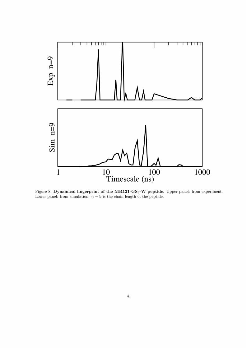
Figure 8: Dynamical fingerprint of the MR121-GS9-W peptide. Upper panel: from experiment.Lower panel: from simulation. n = 9 is the chain length of the peptide.

41

0 20 40 60 80 100 120 140 160 180

Index of Label Positions, from (1-2) to (19-20)

00.10.20.30.40.5

360

ns a

mpl

itude

0 20 40 60 80 100 120 140 160 18000.10.20.30.40.5

126

ns a

mpl

itude

0 20 40 60 80 100 120 140 160 18000.10.20.30.40.5

102

ns a

mpl

itude

0 20 40 60 80 100 120 140 160 18000.10.20.30.40.5

70 n

s am

plitu

de

0 20 40 60 80 100 120 140 160 18000.10.20.30.40.5

64 n

s am

plitu

de

Figure 9: Experimental design. Prediction of the amplitudes of fingerprint peaks of the 5 slowestprocesses in MR121-GS9-W when placing the fluorescence labels at any of the 190 different possibleresidue positions from 1-2 to 19-20. The x-Axis enumerates these 190 labeling positions. The magenta,blue, green, orange, red lines mark the proposed experimental setups to optimally probe the slowest tothe fifth-slowest processes.

42