lable at ScienceDirect

Energy 89 (2015) 435e448

Contents lists avai

Energy

journal homepage: www.elsevier .com/locate/energy

Market and policy risk under different renewable electricity supportschemes

Trine Krogh Boomsma a, Kristin Linnerud b, *

a University of Copenhagen, Department of Mathematical Sciences, 2100 Copenhagen, Denmarkb CICERO Center for International Climate and Environmental Research e Oslo NOe0318 Oslo, Norway

a r t i c l e i n f o

Article history:Received 5 December 2014Received in revised form16 May 2015Accepted 19 May 2015Available online 2 July 2015

Keywords:Renewable energyPolicy uncertaintyGreen certificatesFeed-in tariffsIrreversible investmentsReal options

* Corresponding author. Tel.: þ47 94873338.E-mail addresses: trine@math.ku.dk (T.K. Booms

uio.no (K. Linnerud).

http://dx.doi.org/10.1016/j.energy.2015.05.1140360-5442/© 2015 Elsevier Ltd. All rights reserved.

a b s t r a c t

Worldwide, renewable electricity projects are granted production support to ensure competitiveness.Depending on the design of these support schemes, the cash inflows to investment projects will be moreor less exposed to fluctuations in electricity and/or subsidy prices. Furthermore, as renewable electricitytechnologies mature, there is a possibility that the current support scheme will be terminated or revisedin ways that make it less generous or more in line with market mechanism.

Using a real options approach, we examine how investors in power projects respond to such marketand policy risks. We show that: (1) due to price diversification, the differences in market risk betweensupport schemes like tradeable green certificates, feed-in premiums and feed-in tariffs are less thancommonly believed; (2) the prospects of termination will slow down investments if it is retroactivelyapplied, but speed up investments if it is not; and, (3) this policy uncertainty may add a substantial riskto investments, especially in the first case where investors expect future curtailment of subsidies to affectnew and old installations alike. We conclude the paper by discussing the division of risk betweeninvestor and government.

© 2015 Elsevier Ltd. All rights reserved.

1. Introduction

At present, many renewable electricity projects are grantedproduction support to ensure competitiveness. These supportschemes can be either quantity-driven (the government sets thequantity of new renewable electricity production and lets themarket determine the subsidy level) or price-driven (the govern-ment sets the subsidy level and lets the market determine thequantity). An example of a quantity-driven scheme is a quota sys-tem, in which green certificates are issued to producers in pro-portion to the volume of renewable electricity generated andtraded to satisfy a quota for renewable electricity. Other commonterms for the same concept are ”renewable portfolio standard” and”renewables obligation”. A feed-in scheme is an example of a price-driven scheme, and it can be implemented as either a tariff thatreplaces the electricity price or as a price premium paid on top ofthis price. As of 2013, 71 countries had implemented price-driven

ma), kristin.linnerud@cicero.

support schemes and 24 countries had implemented quantity-driven schemes.1

Depending on the design of these support schemes, the cashinflows to investment projects will be more or less exposed tofluctuations in electricity and/or subsidy prices. In addition to thismarket risk is the risk that the policy will change in the future. Asrenewable electricity technologies mature, governments mayeventually want to terminate these support schemes or revise themin ways that make them less generous. The prospect of revisedrenewable electricity support schemes in the EU post 2020 mayserve as an example. Most EU member states support the produc-tion of electricity using renewable energy sources by offering fixedfeed-in tariffs for a given number of years. Because these feed-intariffs have systematically exceeded the marginal costs of renew-able electricity production, in 2012 the tariffs for new plants werecut significantly (e.g., Germany) or removed (e.g., Spain). Moreover,Spain, Belgium, the Czech Republic, Bulgaria and Greece haverecently enacted retroactive adjustments to their feed-in tariffs,

1 Source: REN 21 Renewable Energy Policy Network for the 21st Century, GSRPolicy Table. [http://www.ren21.net/RenewablePolicy/GSRPolicyTable.aspx, 16th ofFebruary 2014.].

T.K. Boomsma, K. Linnerud / Energy 89 (2015) 435e448436

thereby reducing the profitability of already installed plants [7].Furthermore, a greater influx of intermittent renewable electricityfunded by fixed feed-in tariffs challenges the functioning of powermarkets. In a communication on the internal energy market pub-lished in November 2012, the EU Commission suggests that thesupport schemes are revised to better reflect market mechanisms.

We examine how such market and policy uncertainties affectinvestment decisions in the renewable electricity sector. Thebenchmark case is a situation in which investors expect the currentsupport scheme to stay the same indefinitely. We assume that in-vestors receive an electricity price and a subsidy payment for eachunit of electricity produced. We allow for different combinations ofdeterministic and stochastic, geometric Brownian motion diffusionprocesses. The resulting models can be used to evaluate supportschemes of tradable green certificates (both prices are stochastic),feed-in premiums (a stochastic electricity price and a deterministicsubsidy payment) and feed-in tariffs (only a deterministic subsidypayment). We further assume that at some random point in time,the subsidy payment will be terminated, and that investors eitherexpect or do not expect that this decision will be retroactivelyapplied. This is modeled by including a Poisson jump process.

We formulate the investment decision as a real option probleminwhich the option to delay an irreversible investment decision hasa value [8]. Our optimization problems are solved analytically usingdynamic programming. The essence of this method is to comparethe value of immediate investment with the expected value ofdelaying the investment decision. In our case, finding the optimaltiming of an investment implies identifying the sum of the elec-tricity price and the subsidy paymentdthe threshold revenue-dthat defines the border between the continuation region (inwhich the optimal decision is to wait) and the stopping region (inwhich the optimal decision is to invest). Uncertainty will affect thevalue of the option to wait and therefore this threshold.

Taking the perspective of an energy firm, real options theory hasbeen used to derive the optimal investment and operative decisionsunder uncertain policy conditions. Most studies aim at correctlymodeling the market-driven sources of uncertainty under specificpolicy schemes, like the carbon price process under the EU emis-sion trading scheme (e.g. Refs. [10,12,15,19,26,29e31]. Some studiesacknowledge that policy uncertainty could be modeled moredrastically. This can be done by including stochastic jumps in theprices of policy instruments reflecting sudden changes in the policytarget (e.g. Refs. [28,11], or by modeling the risk that a scheme willbe introduced (e.g. Ref. [16], or that an existing scheme will bereplaced (e.g,. Ref. [4] and Ref. [23] or simply removed (e.g.Refs. [2,3,24]. analyze policy uncertainty from a different perspec-tive. They examine the uncertainties arising from public support forrenewable energy and show how these uncertainties generate realregulatory options, not in the hands of the project's promoter, thatreduce the net present value of the project. Finally, a few studieshave used project-level data to test whether energy firms time theirdecisions as predicted by real options models under uncertainpolicy conditions [16,25]. These empirical studies find that uncer-tain policy and regulatory conditions significantly affect the patternof development in the electric power industry.

The nearest papers apparently to ours are Boomsma et al. [4]and Ref. [2]. Boomsma et al. [4] examine investment timing andcapacity choice under uncertainty in capital costs, electricity priceand subsidy payments under different renewable electricity sup-port schemes, and the possibility of a change from one supportscheme to another. Using simulations they find that feed-in tariffsencourage earlier investments than feed-in premiums and greencertificates [2]. derive the investment timing for a renewable en-ergy facility with price and quantity uncertainty, where theremightbe a subsidy proportional to the quantity of production. Including

the possibility that the subsidy is retroactively terminated, theyconclude that a subsidy, even one having an unexpected with-drawal, will hasten investment compared to a situation with nosubsidy. Like Boomsma et al. [4] we allow for more than one sto-chastic price process in order to realistically model the supportschemes in use.We extend their analysis by allowing for correlationin prices to better investigate the risk of green certificates underdifferent assumptions of price dependencies. In order to moreclearly convey how individual price and policy uncertainties arerelated to the threshold revenue, we choose to derive the solutionanalytically following an approach developed in Ref. [1] andapplied in Ref. [2]. Like [2] we examine the prospects of schemetermination; but we reach a somewhat different conclusion thanRef. [2] because we compare and contrast situations where in-vestors believe this decision will be retroactively applied or not.

Real options studies that have derived analytical solutions forcases with two, possibly correlated, geometric Brownian motiondiffusion processes include the classical reference by Ref. [20]. Theyexamine the perpetual American option to pay a stochastic cost Iagainst a project of stochastic value S. The option value function ishomogenous of degree one and thus the investment rule issimplified to wait until S/I reaches a constant threshold value [1].extend this model to a two dimensional real options problemwhere the option value function is not homogenous of degree oneand, as a consequence, it is not possible to reduce the dimension-ality down to one. More specifically, they examine the perpetualAmerican option to pay a constant cost I against the net cash flowS�K where both cash flows follow, possibly correlated, geometricBrownian motion processes. They develop an implicit representa-tion of the investment boundary as the solution to a set of nsimultaneous equations in nþ1 unknown variables and parameters.By fixing one of the random variables, say S, they derive a thresholdvalue for the other random variable K as a function of the first. Weuse their approach to examine a similar problem; to pay a fixed costI against the sum of two, possibly correlated, price processes SþK.We show that the optimal threshold provides a non-linear relationbetween these two random variables.

Merton, (1976) [22] was the first to construct an option pricingformula where the value of the underlying asset is generated by amixture of both jump and diffusion processes. Later real optionstudies have applied Merton's jump-diffusion model to processesinvolving sudden death, birth and change of the value of the un-derlying asset (e.g. Refs. [2,5,8,27]. Our study builds upon Ref. [8]who examine the prospects of an introduction or termination ofan investment tax credit. In contrast to Ref. [8]; we assume thatpolicy change is permanent; that is, once the support scheme isterminated, it is never altered. This is the same set-up as in Refs.[2,27]. However, by assuming that investors either expect or do notexpect that these changes will be retroactively applied, we showthat including jump mechanisms may increase but also decreasethe value of waiting.

Our choice of price processes results in a threshold revenuewithimportant characteristics. In cases where both prices are random,such as tradable green certificates, the optimal threshold revenue isa convex function of the observed electricity (subsidy) price.Consequently, as long as the electricity and subsidy prices are notperfectly correlated, part of their individual risks will be diminishedthrough diversification when they are combined. One may arguethat the electricity and certificate prices are negatively correlated(see Refs. [13,17], in which case the gains from risk diversificationmay be substantial. It follows that the market risk and therefore thethreshold revenue may be higher but also lower under a quantity-driven scheme as compared with a price-driven scheme. Byincluding a Poisson jump process, we add further characteristics tothe optimal investment threshold. The prospects of termination

T.K. Boomsma, K. Linnerud / Energy 89 (2015) 435e448 437

will raise the threshold revenue and thus slow down investments ifit is retroactively applied, but lower the threshold revenue and thusspeed up investments if it is not. Thus, policy uncertainty may add asubstantial risk to investments, especially in the first case whereinvestors expect future curtailment of subsidies to affect new andold installations alike.

In the next sectionwe show how uncertainty is modelled. In thethird and fourth sections we derive the threshold revenue analyt-ically for different support schemes and different uncertainty as-sumptions. In the fifth section we illustrate these analyticalsolutions with a numerical example for a wind power project. Wediscuss policy implications in the final section.

3 For many renewable energy sources, production is completely determined bythe weather conditions and may be highly varying on hourly, daily and seasonaltime scales. Variations are usually smaller on a yearly time scale, which justifies theassumption of constant expected production.

2. Market and policy uncertainty

We distinguish between two types of uncertainty: market un-certainty and policy uncertainty. Market uncertainty relates toelectricity prices and subsidy payments, and evolves continuouslyover time. In contrast, policy uncertainty, such as future termina-tion of the current support scheme, occurs at discrete points intime.

When modeling market uncertainty, we let electricity pricesðStÞt�0 and subsidy payments ðKtÞt�0 follow geometric Brownianmotion processes such that

dSt ¼ mSStdt þ sSStdzSt ; (1)

dKt ¼ mKKtdt þ sKKtdzKt : (2)

Here, mS,mK and sS,sK are constants that represent the trends andvolatilities of prices and payments, respectively, and dzSt,dzKt arestandard Brownian motions with E½dzStdzKt � ¼ rdt. Hence, currentvalues of the stochastic processes are known,whereas future valuesare log-normally distributed with means, variances and covariancethat grow linearly with time. In the following presentation, wemayoccasionally refer to subsidy payments as subsidy prices.

This definition of market uncertainty covers various marketdesigns. The subsidy may be paid out either as a substitute for theelectricity price (St≡0) or in addition to this price (St>0). We willspecifically focus on risk exposure related to both processes, and soour real options problem is bivariate. We will also derive solutionsfor the cases where the producer faces variations in one price(univariate real options problem) or in none of the prices (deter-ministic problem).

Remark 1. A support scheme for which sK¼ 0 is usually referredto as feed-in tariff (St≡0) or a feed-in premium (St>0). A schemewith sS>0 and sK>0 and St>0 and Kt>0 can be viewed as a certifi-cate trading scheme, in which certificate prices represent thesubsidy payments.

We model policy uncertainty as a Markov process ðdtÞt�0 withstates {0,1} such that

dt ¼�1; if apolicy changehasoccured in the time interval ½0;tÞ;0; otherwise;

(3)

with d0¼ 0. The jump-intensities of the Markov process are deno-ted by lij, where we assume that

2 The probability that a jump occurs during a short time interval dt is in factldtþo(dt), where o(dt) is a term of order less than dt. In accordance with real op-tions theory, we ignore o(dt).

lij ¼�l; if i ¼ 0; j ¼ 1;0; if i ¼ 1; j ¼ 0;

(4)

for constant l>0. Roughly speaking, ddt¼ 1; that is, a change ofpolicy occurs during a short time interval dt, with probability ldt.2

Furthermore, if dt�¼0 (t� denotes the left-hand limit of t), thendt¼ 0 with probability 1�ldt, and if dt�¼1, then dt¼ 1 with prob-ability 1, such that 1 is an absorbing state. We assume that policychange is independent of the evolution of electricity prices andsubsidy payments.

Remark 2. We motivate policy change by advances in technology.In particular, governments may eventually decide to terminate thecurrent support scheme as renewable electricity technologiesbecome increasingly mature. For this reason, we assume that oncethe support scheme has been terminated, it is never re-introduced.

3. Support scheme with an infinite lifespan

We start by valuing an operating renewable electricity projectthat is entitled to a deterministic or stochastic subsidy throughoutthe lifetime of the project.

The project lifetime is finite and denoted by T. We assumeconstant expected production.3 If profit scales with production, thisimplies we can value a single unit of production. We consider aprice-taking producer, whose instantaneous per unit revenue isgiven by the sum of the electricity price and a subsidy payment. Ifoperating costs are constant, these can be incorporated into theinvestment costs, and to simplify the presentation, we thereforedisregard these costs. We denote the required rate of return of theproject by r4 and assume that r>mS and r>mK. Without these as-sumptions, investment may never occur.

We denote the value of the project by V(S,K), which is a functionof the current electricity price S and subsidy payment K. This valueis the expected present value of future revenues over the project'slifetime, that is,

VðS;KÞ ¼ E

24ZT

0

e�rtðSt þ KtÞdtjS0 ¼ S;K0 ¼ K

35 :¼ rSSþ rKK;

(5)

where we define

rS¼ZT0

e�ðr�mSÞtdt¼1�e�ðr�mSÞT

r�mS; rK¼

ZT0

e�ðr�mK Þtdt¼1�e�ðr�mK ÞT

r�mK;

(6)

see Appendix B.1 for the derivation. In spite of the correlation be-tween electricity prices and subsidy payments, the project value isadditive. Also, note that the result continues to hold if mK¼ 0, sK¼ 0and/or St≡0. Finally, we let investment costs be constant and denotethese by I, such that the net present value of the project is V(S,K)�I.

4 Many asset pricing papers apply risk-neutral valuation, assuming marketcompleteness. Under this assumption, the discount rate reflects the required rate ofreturn on projects with similar risk. However, electricity markets may be far fromcomplete due lack of suitable hedging instruments for volume risk, policy risk etc.For this reason, we assume an exogenously given discount rate.

T.K. Boomsma, K. Linnerud / Energy 89 (2015) 435e448438

The value of the investment option W(S,K) is also a function ofthe state variables S and K. Assuming that our option to invest hasan infinite lifespan, we obtain a time-homogeneous value processand time does not need to be a state variable. The investment op-tion value is the expected net present value of the project at theoptimal time of investment. Because the underlying stochasticprocesses are Markovian, the value function satisfies the Bellmanequation

WðS;KÞ ¼ max�VðS;KÞ � I;

11þ rdt

E½WðSþ dS;K þ dKÞjS;K��:

(7)

According to the Bellman equation, at any point in time, theinvestor decides whether to invest in the project or continue todelay investment. By applying Ito’s lemma (see Ref. [14]) to expandthe expectation, and rearranging terms, we arrive at the followingsecond order homogenous partial differential equation (PDE),which holds when continuation is optimal

12

s2SS

2v2WvS2

þ s2KK2v

2WvK2 þ 2sSsKrSK

v2WvSvK

!

þ mSSvWvS

þ mKKvWvK

� rW ¼ 0:

(8)

Intuitively, this PDE requires that the expected rate of return oninvestment equals the discount rate. It is subject to conditions atthe boundary at which investment becomes optimal.

To solve the PDE, we assume a generic solution of the form

WðS;KÞ ¼ bSaSKaK ; (9)

in which S>0 and K>0.5

Remark 3. . If the value function had been homogenous of degreeone, the solution could be shown to have this form (see Ref. [20].6 Inour case, however, the value of the project is not homogenous ofdegree one, and therefore our bivariate real options problemcannot be reduced to a univariate real options problem. Instead wefollow a quasi-analytical approach developed by Ref. [1] for anequivalent problem to ours, and applied in Ref. [2].

For the above expression to be a solution, aS and aK must satisfythe equation Q (aS,aK)¼0, where

Q ðaS;aKÞ ¼12

�s2SaSðaS � 1Þ þ s2KaKðaK � 1Þ þ 2sSsKraSaK

�þ mSaS þ mKaK � r:

(10)

This is the equation of an ellipse that is present in all fourquadrants of the plane.7 For the investment value to be increasing

5 This solution covers a situation with two stochastic prices following a geo-metric Brownian Motion. For support schemes with only one stochastic price (forinstance a feed-in premium scheme in which sK¼ 0) or no stochastic price (forinstance a feed-in tariff scheme in which S¼ 0 and sK¼ 0), the optimizationproblem degenerates to a lower dimension real option problem. The solutions tothese problems are shown at the end of Section 3. The numerical illustrations inSection 5 show that when K(S) approach zero, the resulting threshold revenue fortwo stochastic prices S and K approach the same value as for one stochastic price S.Equivalently, when S approach zero, the resulting threshold revenue for one sto-chastic price S approach the same value as for no stochastic price.

6 [20] show that if the value function is homogenous of degree one, then one canlet W(S,K)¼Sw(s),s¼ K/S for some function wð,Þ and reduce the PDE for the two-factor problem to a one-factor PDE.

7 Note that for aS¼ 0 or aK¼ 0, the equation reduces to the quadratic equation ofthe standard one-factor PDE from real options analysis. This equation is known tohave a positive and a negative root (see Ref. [8].

in both prices, we restrict attention to solutions in the first quad-rant; that is, we assume that aS� 0 and aK� 0.

When investment is optimal, the option value equals the netpresent value of the project W(S,K)¼ rSSþrKK�I. Hence, theboundary conditions are

bSaSKaK ¼ rSSþ rKK � I; baSSaS�1KaK ¼ rS; baKS

aSKaK�1 ¼ rK ;

(11)

where S and K must be the prices at which investment is optimal(i.e. threshold prices). The first equality is the value matchingcondition and the second and third equalities are the so-calledsmooth pasting conditions (see Ref. [8]. With Q ðaS;aKÞ ¼ 0, weobtain four equalities in the five unknowns (aS,aK,b,S,K), and so thethreshold prices define a one-dimensional subset of S�K-space. Byfixing S andmanipulating the boundary conditions, we arrive at thefollowing result.

Proposition 1. Assume that mSs0∨sS>0 and mKs0∨sK>0. GivenS>0, the optimal time t to invest is the first time Kt� K*(S),where K*(S)is determined by the following equalities

S ¼ aS

aS þ aK � 1$IrS; K�ðSÞ ¼ aK

aS þ aK � 1$IrK;

Q ðaS;aKÞ ¼ 0; aS;aK � 0:(12)

Remark 4. . Note that we may fix either S or K such that theoptimal time t to invest is the first time Kt� K*(K) or St� S*(K). Inmost cases, we present the threshold as K*(S), reflecting therequired subsidy payment to trigger investment. In the case of afixed subsidy payment, however, we present the threshold as S*(K)following the standard of real options analysis, in which thethreshold relates to the stochastic process. From a policy perspec-tive, one may be interested in the total revenue required to triggerinvestment. Thus, for a given electricity price S, we present SþK*(S)when we obtain the thresholds numerically in Section 5.

When investment is optimal, we find that

b¼ 1SaSK�ðSÞaK

$I

aSþaK�1¼ðaSþaK�1ÞaSþaK�1

aaSS a

aKK

$raSS raK

K

IaSþaK�1 ; (13)

with b>0.For aK¼ 0, note the similarity of the result in Proposition 1 to a

univariate real options problem of the type in Ref. [8]. Thus, theabove result for two uncertainty factors is the natural extension ofthe one-factor problem.

Because there is a value of delaying investment, the expectedpresent value of future revenue revenues must exceed investmentcosts to trigger investment in a case with two uncertainty factors.

3.1. Corollary 1

rSSþ rKK�ðSÞ ¼ aS þ aK

aS þ aK � 1$I> I: (14)

See Appendix C.1 for the proof.In Proposition 1, the investment threshold K*(S) depends on S

through the equation Q ðaS;aKÞ ¼ 0. It can, however, be stated inanother way. For a given price S, let

hðSÞ ¼ I � rSSrSS

: (15)

T.K. Boomsma, K. Linnerud / Energy 89 (2015) 435e448 439

Then, the optimal time t to invest is the first time Kt� K*(S),where

K�ðSÞ ¼ ahðSÞ þ 1aðhðSÞ þ 1Þ$

IrK; Q ða;ahðSÞ þ 1Þ ¼ 0; a;ahðSÞ þ 1 � 0:

(16)

This is instructive in the sense that for a given electricity price S,we can isolate the subsidy payment required to trigger investment.

For completeness, we provide the solutions to the univariatereal options problem that arise with a fixed price premium and tothe deterministic problem with a fixed tariff.

Fixed feed-in premium When subsidies are paid out as a con-stant price premium K, i.e. mK¼sK¼ 0 and St>0, the optimal time t toinvest is the first time St� S*(K), where

S�ðKÞ ¼ aS

aS � 1$I � rKK

rS; Q SðaSÞ ¼ 0; (17)

with Q SðaSÞ :¼ Q ðaS;0Þ and we assume that rKK<I; that is, thesubsidy payment is not by itself sufficient to justify investment.

Fixed feed-in tariff When subsidies are paid out as a constanttariff K (i.e mK¼sK¼ 0 and St≡0) immediate investment is optimal ifand only if

rKK � I; (18)

which is also known as the net present value (NPV) rule.

4. Termination of the support scheme

We now analyze the prospect that at a random point in time thecurrent support scheme may be terminated. We distinguish be-tween two cases. The investor either believes that government maydecide not to enter into new contracts but will commit to existingones (i.e., there is no retroactive termination of subsidy payments),or it may decide neither to enter into new contracts nor to committo existing ones (i.e., subsidy payments are terminatedretroactively).

In valuing the project and investment, we consider two regimes:Regime 0, in which termination has not yet occurred, and regime 1,in which the support scheme has already been terminated.Accordingly, we denote the project value in regimes 0 and 1 byV0(S,K) and V1(S,K), respectively, and likewise for the value of theinvestment option.

Again, the value of an operating project is the expected presentvalue of future revenues. In regime 0, revenues from electricityprices continue throughout the project lifetime, but subsidy pay-ments may be terminated at a random point in time. In regime 1,revenues stem from electricity prices only. Hence,

V0ðS;KÞ ¼ E

24ZT

0

e�rt�St þ Kt1fdt¼0g�dtjS0 ¼ S;K0 ¼ K; d0 ¼ 0

35 :

¼ rSSþ rK0ðlÞK;(19)

V1ðSÞ ¼ E

24ZT

0

e�rtStdtjS0 ¼ S; d0 ¼ 1

35 ¼ rSS; (20)

where rS is defined as above and

rK0ðlÞ ¼ZT0

e�ðrþl�mK Þtdt ¼ 1� e�ðrþl�mK ÞT

r þ l� mK; (21)

see Appendix B.2 for the derivation. Without retroactive termina-tion, we use the compounding factor rK0(l), where l¼0; whereaswith retroactive termination, we use rK0(l), where l>0. Conse-quently, the project value in regime 0 will be lower if investorsexpect the termination to be retroactively applied than if investorsexpect the termination decision to only affect future installations.

The value of the investment option must satisfy the followingBellman equations:

W0ðS;KÞ ¼ max�V0ðS;KÞ � I;

1� ldt1þ rdt

E½W0ðSþ dS;K þ dKÞjS;K�

þ ldt1þ rdt

E½W1ðSþ dSÞjS��;

(22)

W1ðSÞ ¼ max�V1ðSÞ � I;

11þ rdt

E½W1ðSþ dSÞjS��: (23)

Whether in regime 0 or 1, at any point in time, the investordecides whether to invest in the project or continue to delay in-vestment. In regime 0, new investment is entitled to subsidies, andthe investment value depends on both electricity prices and sub-sidy payments. If continuation is optimal, the probability that thesupport schemewill be terminated during a short time interval dt isldt, whereas the probability that it will not is 1�ldt. In regime 1,new investment is no longer entitled to subsidies and future rev-enues stem from electricity prices only.

By applying Ito’s lemma and rearranging terms, we obtain thefollowing system of second order PDEs, which holds whencontinuation is optimal

12

s2SS

2v2W0

vS2þ s2KK

2v2W0

vK2 þ 2sSsKrSKv2W0

vSvK

!

þ mSSvW0

vSþ mKK

vW0

vK� lðW0 �W1Þ � rW0 ¼ 0;

(24)

12s2SS

2v2W1

vS2þ mSS

vW1

vS� rW1 ¼ 0: (25)

In regime 0, the expected rate of return on the investment de-creases because of the risk of termination, which produces anadditional term in the PDE. Hence, for a given discount rate, ahigher expected rate of return is required to off-set terminationrisk.

To derive a solution to this system of PDEs, we define theequations

Q 0ðaS;aKÞ ¼12

�s2SaSðaS � 1Þ þ s2KaKðaK � 1Þ þ 2sSsKraSaK

�þ mSaS þ mKaK � ðr þ lÞ;

(26)

Q 1ðaSÞ ¼12s2SaSðaS � 1Þ þ mSaS � r: (27)

The derivations can be found in Appendix D.1 and provide thefollowing result:

Proposition 2. Assume that l>0, mSs0∨sS>0 and mKs0∨sK>0.Then,

T.K. Boomsma, K. Linnerud / Energy 89 (2015) 435e448440

1. The optimal time t1 to invest under regime 1 is the first timeSt1 � S1, where8

S1 ¼ aS1 $I; Q 1ðaS1Þ ¼ 0; aS1 � 0: (28)

aS1 � 1 rS

2. Moreover, given S>0, the optimal time t0 to invest under regime 0 isthe first time Kt0 � K0ðSÞ, where K0(S) is determined by thefollowing equalities

S ¼ aS0

aS0 þ aK0 � 1$IrS$

1þ aS1ðaK0 � 1Þ þ aS0

aS0�aS1 � 1

� $

�SS1

aS1

!;

(29)

K0ðSÞ ¼aK0

aS0 þ aK0 � 1$

IrK0ðlÞ

$

�1�

�SS1

aS1;

Q 0ðaS0;aK0Þ ¼ 0; aS0;aK0 � 0:(30)

Under regime 1, the support scheme has been terminated, and theproblem is a univariate real options problem. For aK0¼ 0, the problemlikewise reduces to a univariate one under regime 0.

As above, to trigger investment, the expected net present value offuture revenues must exceed investment costs, and hence at theboundary we have.

4.1. Corollary 2

Assume that S� S1. Then,

rSSþ rK0ðlÞK0ðSÞ> I: (31)

The proof can be found in Appendix C.2.As above, we state an alternative formulation of Proposition 2.

For a given S>0, let

hðSÞ ¼ ðI � rSSÞ�aS1 � 1

�SaS11 þ ISaS1

rSS�aS1 � 1

�SaS11 � aS1ISaS1

: (32)

Then, the optimal time t to invest is the first time Kt� K0(S),where we can isolate K0(S) such that

K0ðSÞ ¼ahðSÞ þ 1aðhðSÞ þ 1Þ$

IrK0ðlÞ

$

�1�

�SS1

aS1; (33)

Q 0ða;ahðSÞ þ 1Þ ¼ 0; a;ahðSÞ þ 1 � 0: (34)

Fixed feed-in premium As above, when mK¼sK¼ 0 and St>0, theoptimal time t to invest under regime 1 is the first time St� S0(K),where

S0ðKÞ¼aS0

aS0�1$I�rK0ðlÞK

rSþ aS0�aS1

ðaS0�1ÞðaS1�1Þ$IrS$

�S0ðKÞS1

aS1

;

Q S0ðaS0Þ¼0;

(35)

where Q S0ðaKÞ :¼ Q 0ð0;aKÞ and assuming rK0(l)K<I.Assuming the subsidy payment alone is not sufficient to justify

investment, we can show the existence of the investment threshold

8 The quadratic equation Q 1ðaS1Þ ¼ 0 has the root

aS1 ¼ 1=2� mS=s2S þ

ffiffiffiffiffiffiffiffiffiffiffiffiffiffiffiffiffiffiffiffiffiffiffiffiffiffiffiffiffiffiffiffiffiffiffiffiffiffiffiffiffiffiffiffiffiffiffiffiffiffiffið1=2� mS=s

2S Þ2 þ 2r=s2S

q; with aS1>1.

S0(K) and compare it with the threshold under a support schemewith an infinite lifespan S*(K) and that under the risk of terminationS1:

4.2. Corollary 3

Assume that mK¼sK¼ 0 and rK0(l)K<I. Then.

1. Eq. (35) has a unique root in (0,S1).2. If rK0(l):¼rK0(0), then S0(K)<S*(K)<S1.

The proof can be found in Appendix C.3.We see that, under a fixed price premium without retroactive

termination upon investment, the risk of termination always re-duces the required electricity price to trigger investment, andtherefore speeds up the investment rate. We show numerically thatthis is also the case under a certificate trading scheme withoutretroactive termination. Under a subsidy scheme with retroactivetermination risk, our numerical analysis likewise shows that theprospect of termination in most cases reduces the threshold andspeeds up investment, but there are cases in which investmentslows down.

Fixed feed-in tariff When mK¼sK¼ 0 and St≡0, immediate in-vestment is optimal if and only if

rK0ðlÞK � I; (36)

which is again the NPV rule.

5. Numerical solutions

In this sectionwe obtain the threshold revenues numerically fora wind power project. The thresholds are obtained for given valuesof the electricity price S using Propositions 1 and 2 (green certifi-cates), Eqs. (4) and (6) (feed-in premiums) and Eqs. (5) and (7)(feed-in tariffs). The benchmark is a support scheme that investorsbelieve will never be altered. We then examine how investorschange their behavior if they suspect that the current supportschemewill be terminated at a future unknown point in time. Morespecifically, we examine under what circumstances such changes inexpectations will decrease (increase) the threshold revenuerequired to invest relative to the benchmark case and thus increase(decrease) the investment rate. Our examinations are conductedassuming that investors either believe the changes will be appliedretroactively or they do not.

5.1. Case study

The parameter values used in the numerical illustrations beloware presented in Table 1. The project life and investment cost of awind power installation are set equal to T¼ 20 years and I¼ 0.7EUR/kWh. These numbers are representative for a typical 2 MWwind turbine under average wind speeds in Europe [9]; pages9e10).9 The investment cost estimate reflects both investmentcosts (approximately 75% of total costs) and operation and main-tenance costs (approximately 25% of total costs) and is derivedusing a risk-adjusted nominal discount rate of 7.5%. We use realvalues in our optimization problem. Thus, when we let I be fixedover time, we implicitly assume that the nominal investment costgrows with the general price level. The risk adjusted real discount

9 A more recent study by Ref. [21] of the potential for and cost of onshorewindpower installations in Germany confirms concludes that total generation costsare 5e15 EURc/kWh which is equal to an upfront cost of 0.5e1.5 EUR/kWh.

Table 1Parameter values.

Parameter Benchmark value Sensitivity values

I Investment cost 0.7 EUR/kWhT Project life 20 yearsr Discount rate 0.05mS Trend parameter electricity prices 0mK Trend parameter subsidy prices 0 þ/� 0.025.sS Volatility parameter electricity prices 0.00 or 0.06 0.16sK Volatility parameter subsidy prices 0.00 or 0.07 0.16r Correlation coefficient 0 þ/� 1.l Policy uncertainty parameter 0 or 0.1 0.2 and 0.05

0.05

0.055

0.06

0.065

0.07

0 0.01 0.02 0.03 0.04 0.05 0.06 0.07

S+K(

S) [E

UR/

kWh]

S [EUR/kWh]

No uncertainty

Price-driven

Quan ty-driven, ρ=+1.0

Quan ty-driven, ρ=0.0

Quan ty-driven, ρ=-1.0

Fig. 1. Threshold revenue functions for different support schemes assuming there is nopolicy risk (l¼0). No uncertainty is illustrated for sK¼sS¼ 0 (e.g. feed-in tariff). Price-driven support schemes are illustrated for sK¼ 0 and sS¼ 0.06 (e.g. feed-in premium).Quantity-driven support schemes are illustrated for sS¼ 0.06 and sK¼ 0.07 anddifferent values of r (e.g. tradable green certificates). Real prices are fixed: mK¼mS¼ 0.

10 Under feed-in schemes, a plant will receive the tariff/premium in effect in theyear of installation, and it is either kept fixed for the entire period or it is fully orpartly adjusted each year for inflation. For an example of details on feed-in tariffs,see Ref. [6].

T.K. Boomsma, K. Linnerud / Energy 89 (2015) 435e448 441

rate is set to r¼ 5.0%, reflecting an inflation rate of 2.5%. We usemS¼mK¼ 0 in the price processes in Eqs. (1) and (2), which impliesthat these prices likewise grow with the general price level.

We use data from the period with tradable green certificates inSweden and Norway to estimate the parameter values for sS, sK andr. The electricity price volatility, sS ¼ 0.06, and the subsidy pricevolatility, sK¼ 0.07, are estimated by the annual standard deviationof the log returns implied by average weekly prices of three-yearforward contracts traded at NASDAQ OMX and Svenska Kraftme-kling, respectively, for the period 1 January 2005 to 30 April 2015.The corresponding correlation coefficient is estimated to 0.04, butfor convenience we set the benchmark value equal to zero. We alsoinclude numerical illustrations using other parameter values. Forexample, we illustrate the impact of higher volatilities by settingsS¼ 0.16. This electricity volatility parameter is estimated by Ref.[16] in a similar fashion as above, but for an earlier period:2001e2010.

In the simulations where policy uncertainty is introduced, weassume that l¼0.1, implying that investors expect the regime shiftto happen in 1/0.1 ¼10 years. We also vary this parameter value, toinvestigate its relative impact on the threshold revenue.

Our model setup assumes that at any point in time t operatingplants receive the same subsidy payment Kt given in Eq. (2), irre-spective of when they were installed. Although this is a realisticfeature for tradable green certificates, it is in conflict with feed-intariff/premium schemes in which the tariff/premium in effect fornew plants is adjusted downward over time to reflect an expecteddecrease in long-run marginal costs as technology matures. How-ever, our setup is suitable for situations in which investors expectthe downward shift in the real feed-in tariff/premium in effect fornew plants to be equal to the expected fall in long-run marginal

costs, that is, E(dK)¼E(dI)/rK. In that case, neither the decline in realinvestment costs nor the corresponding decline in the real tariff/premiums in effect for new plants has to be modeled explicitlybecause we will get the same results by modeling tariffs/premiumsand investment costs as fixed in real values.10

In the remaining subsections, the behavior of the investors is asfollows. Investors observe the current prices S and K. They thencalculate the threshold revenue as a function of the current elec-tricity price, SþK(S), using the appropriate threshold functionderived in Sections 3 and 4. Finally, they decide to invest if thecurrent revenue exceeds the threshold revenue: SþK� SþK(S).

5.2. The benchmark: support scheme with an infinite lifespan

Assuming investors expect the current support scheme never tobe altered (l¼0), the threshold revenue function SþK(S) is given inSection 3. We first consider the situation in which there is nogrowth in the project value (mK¼mS¼ 0). Thus, the value of waiting,and thereby the level of threshold revenue, will depend only onproject value uncertainty. Fig. 1 illustrates the threshold revenuefunction for three different support schemes: feed-in tariff, feed-inpremium and tradable green certificates. For sK¼sS¼ 0, thethreshold is given by the net present value rule and is fixed to0.0554 EUR/kWh. This is also the threshold for the fixed feed-intariff, in which case S¼ 0 and K¼ I/rK, as stated at the end of Sec-tion 3. For sK¼ 0 and sS¼ 0.07, the threshold revenue is given at theend of Section 3; it increases linearly with the electricity price,starting at 0.0554 EUR/kWh for S¼ 0 and ending at 0.0690 EUR/kWh for K(S)¼0. This is the threshold revenue function for a fixedfeed-in premium. For sS¼ 0.07 and sK¼ 0.06, the threshold reve-nue function is given in Proposition 1 and is applicable for tradablegreen certificates. We show the threshold revenues for r ¼ �1,0 or þ1. For r¼0, the threshold revenue is convex in the electricityprice and reaches a minimum at 0.0634 EUR/kWh.

The threshold revenue functions for the three support schemescan be understood by examining the variance of the relative changein project value at time t given by

Var�dVt

Vt

¼ w2

t s2Sdt þ ð1�wtÞ2s2Kdt þ 2wtð1�wtÞrsKsSdt;

(37)

in which wt¼ rSSt/(rSStþrKKt) (Appendix E). It follows thatcombining two stochastic price processes, part of the risk isdiversified away as long as the two price processes are not perfectlycorrelated. If two stochastic price processes are perfectly negatively

0.05

0.06

0.07

0.08

0.09

0.1

0 0.01 0.02 0.03 0.04 0.05 0.06 0.07

S+K(

S) [E

UR/

kWh]

S [EUR/kWh]

Quan ty-driven, μK: - 0.025

Quan ty-driven, μK: - 0.0 %

Quan ty-driven, μK: + 0.025

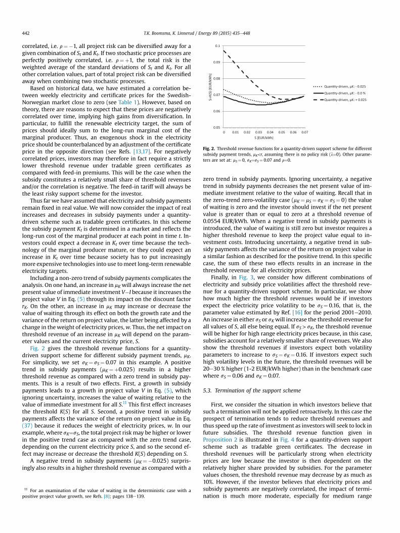
Fig. 2. Threshold revenue functions for a quantity-driven support scheme for differentsubsidy payment trends, mK<r, assuming there is no policy risk (l¼0). Other parame-ters are set at: mS¼ 0, sK¼sS¼ 0.07 and r¼0.

T.K. Boomsma, K. Linnerud / Energy 89 (2015) 435e448442

correlated, i.e. r¼�1, all project risk can be diversified away for agiven combination of St and Kt. If two stochastic price processes areperfectly positively correlated, i.e. r¼þ1, the total risk is theweighted average of the standard deviations of St and Kt. For allother correlation values, part of total project risk can be diversifiedaway when combining two stochastic processes.

Based on historical data, we have estimated a correlation be-tween weekly electricity and certificate prices for the Swedish-Norwegian market close to zero (see Table 1). However, based ontheory, there are reasons to expect that these prices are negativelycorrelated over time, implying high gains from diversification. Inparticular, to fulfill the renewable electricity target, the sum ofprices should ideally sum to the long-run marginal cost of themarginal producer. Thus, an exogenous shock in the electricityprice should be counterbalanced by an adjustment of the certificateprice in the opposite direction (see Refs. [13,17]. For negativelycorrelated prices, investors may therefore in fact require a strictlylower threshold revenue under tradable green certificates ascompared with feed-in premiums. This will be the case when thesubsidy constitutes a relatively small share of threshold revenuesand/or the correlation is negative. The feed-in tariff will always bethe least risky support scheme for the investor.

Thus far we have assumed that electricity and subsidy paymentsremain fixed in real value. We will now consider the impact of realincreases and decreases in subsidy payments under a quantity-driven scheme such as tradable green certificates. In this schemethe subsidy payment Kt is determined in a market and reflects thelong-run cost of the marginal producer at each point in time t. In-vestors could expect a decrease in Kt over time because the tech-nology of the marginal producer mature, or they could expect anincrease in Kt over time because society has to put increasinglymore expensive technologies into use tomeet long-term renewableelectricity targets.

Including a non-zero trend of subsidy payments complicates theanalysis. On one hand, an increase in mKwill always increase the netpresent value of immediate investment V�I because it increases theproject value V in Eq. (5) through its impact on the discount factorrK. On the other, an increase in mK may increase or decrease thevalue of waiting through its effect on both the growth rate and thevariance of the return on project value, the latter being affected by achange in theweight of electricity prices,w. Thus, the net impact onthreshold revenue of an increase in mK will depend on the param-eter values and the current electricity price, S.

Fig. 2 gives the threshold revenue functions for a quantity-driven support scheme for different subsidy payment trends, mK.For simplicity, we set sK¼ sS¼ 0.07 in this example. A positivetrend in subsidy payments (mK¼þ0.025) results in a higherthreshold revenue as compared with a zero trend in subsidy pay-ments. This is a result of two effects. First, a growth in subsidypayments leads to a growth in project value V in Eq. (5), whichignoring uncertainty, increases the value of waiting relative to thevalue of immediate investment for all S.11 This first effect increasesthe threshold K(S) for all S. Second, a positive trend in subsidypayments affects the variance of the return on project value in Eq.(37) because it reduces the weight of electricity prices, w. In ourexample, where sK¼sS, the total project risk may be higher or lowerin the positive trend case as compared with the zero trend case,depending on the current electricity price S, and so the second ef-fect may increase or decrease the threshold K(S) depending on S.

A negative trend in subsidy payments (mK¼�0.025) surpris-ingly also results in a higher threshold revenue as compared with a

11 For an examination of the value of waiting in the deterministic case with apositive project value growth, see Refs. [8]; pages 138e139.

zero trend in subsidy payments. Ignoring uncertainty, a negativetrend in subsidy payments decreases the net present value of im-mediate investment relative to the value of waiting. Recall that inthe zero-trend zero-volatility case (mK¼ mS¼ sK¼ sS¼ 0) the valueof waiting is zero and the investor should invest if the net presentvalue is greater than or equal to zero at a threshold revenue of0.0554 EUR/kWh. When a negative trend in subsidy payments isintroduced, the value of waiting is still zero but investor requires ahigher threshold revenue to keep the project value equal to in-vestment costs. Introducing uncertainty, a negative trend in sub-sidy payments affects the variance of the return on project value ina similar fashion as described for the positive trend. In this specificcase, the sum of these two effects results in an increase in thethreshold revenue for all electricity prices.

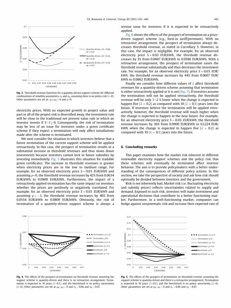
Finally, in Fig. 3, we consider how different combinations ofelectricity and subsidy price volatilities affect the threshold reve-nue for a quantity-driven support scheme. In particular, we showhow much higher the threshold revenues would be if investorsexpect the electricity price volatility to be sS¼ 0.16, that is, theparameter value estimated by Ref. [16] for the period 2001e2010.An increase in either sS or sKwill increase the threshold revenue forall values of S, all else being equal. If sS> sK, the threshold revenuewill be higher for high range electricity prices because, in this case,subsidies account for a relatively smaller share of revenues.We alsoshow the threshold revenues if investors expect both volatilityparameters to increase to sS¼ sK¼ 0.16. If investors expect suchhigh volatility levels in the future, the threshold revenues will be20e30 % higher (1-2 EUR/kWh higher) than in the benchmark casewhere sS¼ 0.06 and sK¼ 0.07.

5.3. Termination of the support scheme

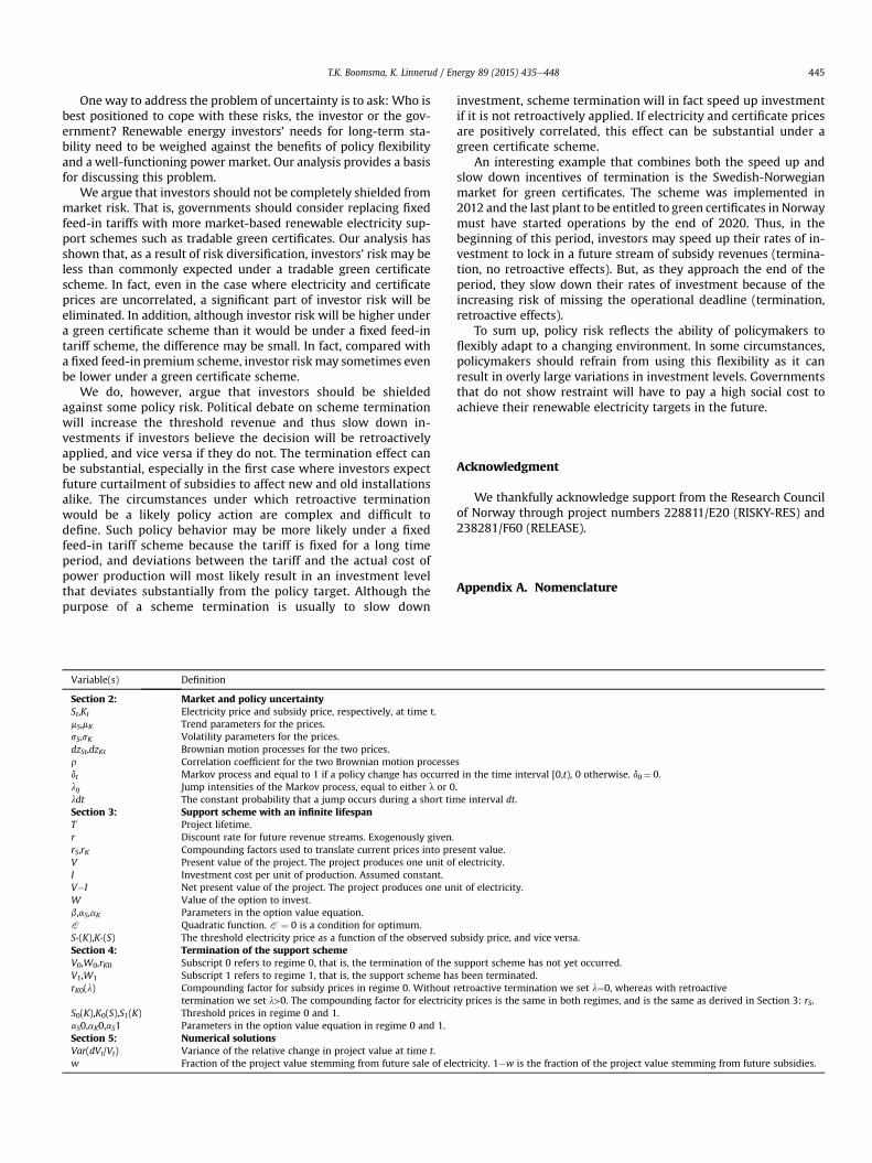
First, we consider the situation in which investors believe thatsuch a termination will not be applied retroactively. In this case theprospect of termination tends to reduce threshold revenues andthus speed up the rate of investment as investors will seek to lock infuture subsidies. The threshold revenue function given inProposition 2 is illustrated in Fig. 4 for a quantity-driven supportscheme such as tradable green certificates. The decrease inthreshold revenues will be particularly strong when electricityprices are low because the investor is then dependent on therelatively higher share provided by subsidies. For the parametervalues chosen, the threshold revenue may decrease by as much as10%. However, if the investor believes that electricity prices andsubsidy payments are negatively correlated, the impact of termi-nation is much more moderate, especially for medium range

0.05

0.06

0.07

0.08

0.09

0.1

0 0.01 0.02 0.03 0.04 0.05 0.06 0.07 0.08 0.09

S +

K(S)

[EU

R/kW

h]

S [EUR/kWh]

Quan ty-driven, σS = 0.06, σK = 0.07

Quan ty-driven, σS = 0.16, σK = 0.16

Quan ty-driven, σS = 0.16, σK = 0.07

Fig. 3. Threshold revenue functions for a quantity-driven support scheme for differentcombinations of volatility parameters, sS and sK, assuming there is no policy risk (l¼0).Other parameters are set at: mS¼mK¼ 0 and r¼0.

T.K. Boomsma, K. Linnerud / Energy 89 (2015) 435e448 443

electricity prices. With no expected growth in project value andpart or all of the project risk is diversified away, the investment rulewill be close to the traditional net present value rule in which aninvestor invests if V�I� 0. Consequently, the risk of terminationmay be less of an issue for investors under a green certificatescheme if they expect a termination will only affect installationsmade after the scheme is terminated.

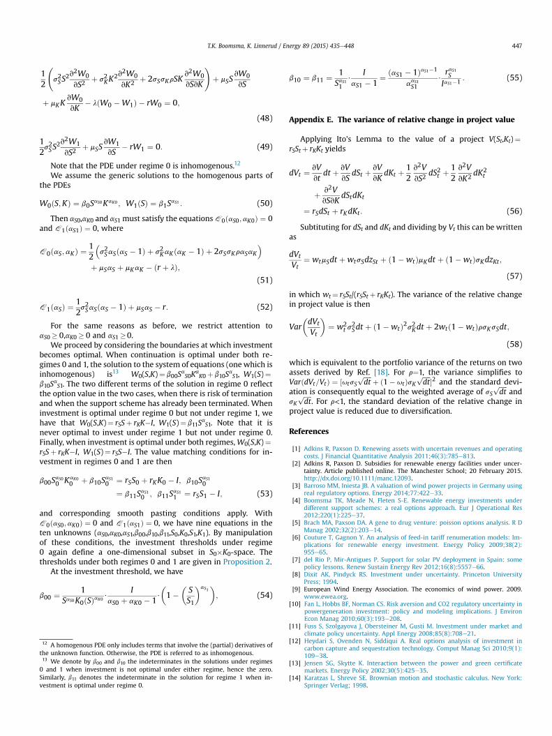
We next consider the situation in which investors believe that afuture termination of the current support scheme will be appliedretroactively. In this case, the prospect of termination results in asubstantial increase in threshold revenues and thus slows downinvestments because investors cannot lock in future subsidies byinvesting immediately. Fig. 5 illustrates this situation for tradablegreen certificates. The increase in threshold revenues is greaterwhen electricity prices are in the low to medium range. Forexample, for an observed electricity price S¼ 0.03 EUR/kWh andassuming r¼0, the threshold revenue increases by 42% from 0.0634EUR/kWh to 0.0900 EUR/kWh. Furthermore, the impact of aretroactively applied termination has the same impact on investorswhether the prices are positively or negatively correlated. Forexample, for an observed electricity price S¼ 0.03 EUR/kWh andassuming r¼�1, the threshold revenue increases by 46% from0.0554 EUR/kWh to 0.0809 EUR/kWh. Obviously, the risk oftermination of a quantity-driven support scheme is always a

0.05

0.06

0.07

0.08

0 0.01 0.02 0.03 0.04 0.05 0.06 0.07

S +

K(S)

[EIR

/kW

h]

S [EUR/kWh]

Termina on: ρ=+1.0

Termina on: ρ=0

Termina on: ρ=-1.0

Benchmark: ρ=+1.0

Benchmark: ρ=0

Benchmark: ρ=-1.0

Fig. 4. The effects of the prospect of termination on threshold revenue assuming thesupport scheme is quantity-driven and there is no retroactive arrangement. Termi-nation is expected in 10 years (l¼0.1), and the benchmark is no policy uncertainty(l¼0). Other parameters are set at mK¼mS¼ 0 and sS¼ 0.06 and sK¼ 0.07.

serious issue for investors if it is expected to be retroactivelyapplied.

Fig. 6 shows the effects of the prospect of termination on a price-driven support scheme (e.g., feed-in tariff/premium). With noretroactive arrangement, the prospect of termination always de-creases threshold revenue, as stated in Corrollary 3. However, inthis case, the impact is negligible. For example, for an observedelectricity price S¼ 0.03 EUR/kWh, the threshold revenue de-creases by 3% from 0.0607 EUR/kWh to 0.0586 EUR/kWh. With aretroactive arrangement, the prospect of termination raises thethreshold revenue substantially and thus decreases the investmentrate. For example, for an observed electricity price S¼ 0.03 EUR/kWh, the threshold revenue increases by 44% from 0.0607 EUR/kWh to 0.0862 EUR/kWh.

Finally we consider how different values of l affect thresholdrevenues for a quantity-driven scheme assuming that terminationis either retroactively applied or it is not (Fig. 7). If investors assumethe termination will not be applied retroactively, the thresholdrevenue will be only 1e2 % lower when the change is expected tohappen five (l ¼ 0.2) as compared with 10 (l ¼ 0.1) years into thefuture. If investors believe the termination will be applied retro-actively, however, the threshold revenue will much higher whenthe change is expected to happen in the near future. For example,for an observed electricity price S¼ 0.03 EUR/kWh, the thresholdrevenue increases by 36% from 0.0900 EUR/kWh to 0.1224 EUR/kWh when the change is expected to happen five (l ¼ 0.2) ascompared with 10 (l ¼ 0.1) years into the future.

6. Concluding remarks

This paper examines how the market risk inherent in differentrenewable electricity support schemes and the policy risk thatthese schemes will eventually be terminated affect investorbehavior. The aim is to provide policymakers with a better under-standing of the consequences of different policy actions. In thissection, we take the perspective of society and ask how risk shouldoptimally be divided between investors and the government.

Risk is not inherently bad. Market risk (i.e. fluctuating electricityand subsidy prices) reflects uncertainties related to supply anddemand. Exposed to such risk, investors will make investment andoperational decisions that contribute to a better functioning mar-ket. Furthermore, in a well-functioning market, companies canhedge against unsystematic risk and increase their expected rate of

0.05

0.06

0.07

0.08

0.09

0.1

0.11

0.12

0.13

0 0.01 0.02 0.03 0.04 0.05 0.06 0.07

S +

K(S)

[EU

R/kW

h]

S [EUR/kWh]

Termina on: ρ=+1.0

Termina on: ρ=0

Termina on: ρ=-1.0

Benchmark: ρ=+1.0

Benchmark: ρ=0

Benchmark: ρ=-1.0

Fig. 5. The effects of the prospect of termination on threshold revenue assuming thesupport scheme is quantity-driven and there is a retroactive arrangement. Terminationis expected in 10 years (l¼0.1), and the benchmark is no policy uncertainty (l¼0).Other parameters are set at mK¼mS¼ 0 and sS¼ 0.06 and sK¼ 0.07.

0.05

0.07

0.09

0.11

0 0.01 0.02 0.03 0.04 0.05 0.06 0.07

S +

K(S)

[EU

R/kW

h]

S [EUR/kWh]

Benchmark

Termina on: no retroac vearrangement

Termina on: retroac vearrangement

Fig. 6. The effects of the prospect of termination on threshold revenue assuming the support scheme is price-driven and there is a retroactive arrangement or there is not.Termination is expected in 10 years (l¼0.1), and the benchmark is no policy uncertainty (l¼0). Other parameters are set at mK¼mS¼ 0 and sK¼ 0 and sS¼ 0.07.

0.05

0.07

0.09

0.11

0.13

0.15

0.17

0 0.01 0.02 0.03 0.04 0.05 0.06 0.07

S +

K(S)

[EU

R/kW

h]

S [EUR/kWh]

Termina on: retroac ve arr., λ=0.2 (5 years)

Termina on: retroac ve arr., λ=0.1 (10 years)

Termina on: retroac ve arr., λ=0.05 (20 years)

Termina on: no retroac ve arr., λ=0.2 (5 years)

Termina on: no retroac ve arr., λ=0.1 (10 years)

Benchmark: λ=0 (no termina on)

Fig. 7. The effects of different values of l on threshold revenue for various termination scenarios for a quantity-driven scheme. Other parameters are set at mK¼mS¼ 0, sS¼ 0.06 andsK¼ 0.07 and r¼0.

T.K. Boomsma, K. Linnerud / Energy 89 (2015) 435e448444

return on investments by increasing their amount of systematicrisk.

Policy risk (i.e. the possibility that the current scheme will berevised or terminated) reflects the ability of policymakers to flexiblyadapt to a changingenvironment.With aflexiblepolicy, policymakers

can respond to improved information on the science of climatechange, the cost and benefits of renewable electricity technologies,political decisions and trends in other countries, the impact of anincreased share of intermittent, renewable energy sources on thepower market, and the need to ensure continued political support.

T.K. Boomsma, K. Linnerud / Energy 89 (2015) 435e448 445

One way to address the problem of uncertainty is to ask: Who isbest positioned to cope with these risks, the investor or the gov-ernment? Renewable energy investors’ needs for long-term sta-bility need to be weighed against the benefits of policy flexibilityand a well-functioning power market. Our analysis provides a basisfor discussing this problem.

We argue that investors should not be completely shielded frommarket risk. That is, governments should consider replacing fixedfeed-in tariffs with more market-based renewable electricity sup-port schemes such as tradable green certificates. Our analysis hasshown that, as a result of risk diversification, investors’ risk may beless than commonly expected under a tradable green certificatescheme. In fact, even in the case where electricity and certificateprices are uncorrelated, a significant part of investor risk will beeliminated. In addition, although investor risk will be higher undera green certificate scheme than it would be under a fixed feed-intariff scheme, the difference may be small. In fact, compared witha fixed feed-in premium scheme, investor risk may sometimes evenbe lower under a green certificate scheme.

We do, however, argue that investors should be shieldedagainst some policy risk. Political debate on scheme terminationwill increase the threshold revenue and thus slow down in-vestments if investors believe the decision will be retroactivelyapplied, and vice versa if they do not. The termination effect canbe substantial, especially in the first case where investors expectfuture curtailment of subsidies to affect new and old installationsalike. The circumstances under which retroactive terminationwould be a likely policy action are complex and difficult todefine. Such policy behavior may be more likely under a fixedfeed-in tariff scheme because the tariff is fixed for a long timeperiod, and deviations between the tariff and the actual cost ofpower production will most likely result in an investment levelthat deviates substantially from the policy target. Although thepurpose of a scheme termination is usually to slow down

Variable(s) Definition

Section 2: Market and policy uncertaintySt,Kt Electricity price and subsidy price, respectively, at time t.mS,mK Trend parameters for the prices.sS,sK Volatility parameters for the prices.dzSt,dzKt Brownian motion processes for the two prices.r Correlation coefficient for the two Brownian motion processedt Markov process and equal to 1 if a policy change has occurrelij Jump intensities of the Markov process, equal to either l or 0ldt The constant probability that a jump occurs during a short timSection 3: Support scheme with an infinite lifespanT Project lifetime.r Discount rate for future revenue streams. Exogenously given.rS,rK Compounding factors used to translate current prices into preV Present value of the project. The project produces one unit ofI Investment cost per unit of production. Assumed constant.V�I Net present value of the project. The project produces one unW Value of the option to invest.b,aS,aK Parameters in the option value equation.Q Quadratic function. Q ¼ 0 is a condition for optimum.S*(K),K*(S) The threshold electricity price as a function of the observed sSection 4: Termination of the support schemeV0,W0,rK0 Subscript 0 refers to regime 0, that is, the termination of theV1,W1 Subscript 1 refers to regime 1, that is, the support scheme harK0(l) Compounding factor for subsidy prices in regime 0. Without

termination we set l>0. The compounding factor for electriciS0(K),K0(S),S1(K) Threshold prices in regime 0 and 1.aS0,aK0,aS1 Parameters in the option value equation in regime 0 and 1.Section 5: Numerical solutionsVar(dVt/Vt) Variance of the relative change in project value at time t.w Fraction of the project value stemming from future sale of ele

investment, scheme termination will in fact speed up investmentif it is not retroactively applied. If electricity and certificate pricesare positively correlated, this effect can be substantial under agreen certificate scheme.

An interesting example that combines both the speed up andslow down incentives of termination is the Swedish-Norwegianmarket for green certificates. The scheme was implemented in2012 and the last plant to be entitled to green certificates in Norwaymust have started operations by the end of 2020. Thus, in thebeginning of this period, investors may speed up their rates of in-vestment to lock in a future stream of subsidy revenues (termina-tion, no retroactive effects). But, as they approach the end of theperiod, they slow down their rates of investment because of theincreasing risk of missing the operational deadline (termination,retroactive effects).

To sum up, policy risk reflects the ability of policymakers toflexibly adapt to a changing environment. In some circumstances,policymakers should refrain from using this flexibility as it canresult in overly large variations in investment levels. Governmentsthat do not show restraint will have to pay a high social cost toachieve their renewable electricity targets in the future.

Acknowledgment

We thankfully acknowledge support from the Research Councilof Norway through project numbers 228811/E20 (RISKY-RES) and238281/F60 (RELEASE).

Appendix A. Nomenclature

sd in the time interval [0,t), 0 otherwise. d0¼ 0..e interval dt.

sent value.electricity.

it of electricity.

ubsidy price, and vice versa.

support scheme has not yet occurred.s been terminated.retroactive termination we set l¼0, whereas with retroactivety prices is the same in both regimes, and is the same as derived in Section 3: rS.

ctricity. 1�w is the fraction of the project value stemming from future subsidies.

T.K. Boomsma, K. Linnerud / Energy 89 (2015) 435e448446

Appendix B. The value of the project

B.1 Support scheme with an infinite lifespan

With infinite life of the support scheme, the project value is

VðS;KÞ ¼ E

24ZT

0

e�rtðSt þ KtÞdtjS0 ¼ S;K0 ¼ K

35

¼ZT0

e�rtE½St jS0 ¼ S�dt þZT0

e�rtE½Kt jK0 ¼ K�dt

¼ SZT0

e�ðr�mSÞtdt þ KZT0

e�ðr�mK Þtdt :¼ rSSþ rKK: (38)

The first equality is based on the observations that conditionalon the initial electricity price the current price is independent ofthe initial subsidy payment, and vice versa.

B.2 Termination of the support scheme

Without retroactive termination upon investment, the projectvalue is unaffected by termination risk. With risk of retroactivetermination, by the same arguments as above, V1(S):¼rSS.Moreover,

V0ðS;KÞ ¼ E

24ZT

0

e�rt�St þ Kt1fdt¼0g�dtjS0 ¼ S;K0 ¼ K

35

¼ZT0

e�rtE½St jS0 ¼ S�dt þZT0

e�rtE½Kt jK0 ¼ K�ℙðdt ¼ 0Þdt

¼ SZT0

e�ðr�mSÞtdt þ KZT0

e�ðrþl�mK Þtdt :¼ rSSþ rK0K:

(39)

Here, we further use that termination risk is independent of thesubsidy payment. The second equality holds since the time totermination is exponentially distributed.

Appendix C. The value of waiting

C.1 Proof of corollary 1

Note that

rSSþ rKK�ðSÞ ¼ aS þ aK

aS þ aK � 1$I: (40)

For the expression on the left hand side to be larger than I, it issufficient to show that aSþaK> 1. To see this, recall that whenaS¼ 0, it is well known from the univariate real options problemthat the positive root of the quadratic equation satisfies aK> 1, andvice versa when aK¼ 0 then aS> 1. Hence, the ellipse defined byQ ðaS;aKÞ ¼ 0 must always be above the line aSþaK¼ 1 in the firstquadrant of the plane.

C.2 Proof of corollary 2

Now

rSSþ rK0ðlÞK0ðSÞ ¼aS0 þ aK0

a þ a � 1$I

S0 K0

þ aS0 þ aK0 � aS1ðaS0 þ aK0 � 1ÞðaS1 � 1Þ$I$

�SS1

aS1

:

(41)

By the same arguments as above, aS0þ aK0> 1 and aS1> 1. IfaS0 þ aK0 � aS1 , then

rSSþ rK0ðlÞK0ðSÞ �aS0 þ aK0

aS0 þ aK0 � 1$I; (42)

and the left hand side is greater than I. If aS0 þ aK0 <aS1 , then

rSSþ rK0ðlÞK0ðSÞ>aS0 þ aK0

aS0 þ aK0 � 1$I þ aS0 þ aK0 � aS1

ðaS0 þ aK0 � 1ÞðaS1 � 1Þ$

I ¼ aS1

aS1 � 1$I;

(43)

and again we obtain the desired.

C.3 Proof of corollary 3

1. We follow the lines of [27]. Let

f ðSÞ ¼ S� aS0

aS0 � 1$I � rK0ðlÞK

rS� aS0 � aS1

ðaS0 � 1ÞðaS1 � 1Þ$IrS$

�SS1

aS1

:

(44)

Then,

f00 ðSÞ ¼ �ðaS0 � aS1ÞaS1

ðaS0 � 1Þ $IrS$

�SS1

aS1

$1S2

; (45)

and since aS0> aS1, f00(S)� 0, that is, f is concave on [0,∞). Further-

more, f(0)< 0, and

f ðS1Þ ¼aS0

aS0 � 1$rK0ðlÞK

rS(46)

which shows that f(S1)> 0. Hence, f must have a unique root in(0,S1). We denote this root by S0(K).

2. Clearly, S*(K)< S1. Since,

f ðS�ðKÞÞ¼ aS0�aS1

ðaS0�1ÞðaS1�1Þ$�I� rKð0ÞK

rS� IrS$

�I� rKð0ÞK

I

aS1;

(47)

we have that f(S*(K))> 0. Hence, S*(K)> S0(K).

Appendix D. Solving the PDEs

D.1 Termination of the support scheme

We repeat the system of second order PDEs, which holds whencontinuation is optimal

T.K. Boomsma, K. Linnerud / Energy 89 (2015) 435e448 447

12

s2SS

2v2W0

vS2þ s2KK

2v2W0

vK2 þ 2sSsKrSKv2W0

vSvK

!þ mSS

vW0

vS

þ mKKvW0

vK� lðW0 �W1Þ � rW0 ¼ 0;

(48)

12s2SS

2v2W1

vS2þ mSS

vW1

vS� rW1 ¼ 0: (49)

Note that the PDE under regime 0 is inhomogenous.12

We assume the generic solutions to the homogenous parts ofthe PDEs

W0ðS;KÞ ¼ b0SaS0KaK0 ; W1ðSÞ ¼ b1S

aS1 : (50)

Then aS0,aK0 and aS1 must satisfy the equations Q 0ðaS0;aK0Þ ¼ 0and Q 1ðaS1Þ ¼ 0, where

Q 0ðaS;aKÞ ¼12

�s2SaSðaS � 1Þ þ s2KaKðaK � 1Þ þ 2sSsKraSaK

�þ mSaS þ mKaK � ðr þ lÞ;

(51)

Q 1ðaSÞ ¼12s2SaSðaS � 1Þ þ mSaS � r: (52)

For the same reasons as before, we restrict attention toaS0� 0,aK0� 0 and aS1�0.

We proceed by considering the boundaries at which investmentbecomes optimal. When continuation is optimal under both re-gimes 0 and 1, the solution to the system of equations (one which isinhomogenous) is13 W0(S,K)¼ b00S

aS0K

aK0þ b10S

aS1, W1(S)¼

b10SaS1. The two different terms of the solution in regime 0 reflect

the option value in the two cases, when there is risk of terminationand when the support scheme has already been terminated. Wheninvestment is optimal under regime 0 but not under regime 1, wehave that W0(S,K)¼ rSSþ rKK�I, W1(S)¼ b11S

aS1. Note that it is

never optimal to invest under regime 1 but not under regime 0.Finally, when investment is optimal under both regimes,W0(S,K)¼rSSþ rKK�I, W1(S)¼ rSS�I. The value matching conditions for in-vestment in regimes 0 and 1 are then

b00SaS00 KaK0

0 þ b10SaS10 ¼ rSS0 þ rKK0 � I; b10S

aS10

¼ b11SaS10 ; b11S

aS11 ¼ rSS1 � I; (53)

and corresponding smooth pasting conditions apply. WithQ 0ðaS0;aK0Þ ¼ 0 and Q 1ðaS1Þ ¼ 0, we have nine equations in theten unknowns (aS0,aK0,aS1,b00,b10,b11,S0,K0,S1,K1). By manipulationof these conditions, the investment thresholds under regime0 again define a one-dimensional subset in S0�K0-space. Thethresholds under both regimes 0 and 1 are given in Proposition 2.

At the investment threshold, we have

b00 ¼ 1SaS0K0ðSÞaK0

$I

aS0 þ aK0 � 1$

�1�

�SS1

aS1; (54)

12 A homogenous PDE only includes terms that involve the (partial) derivatives ofthe unknown function. Otherwise, the PDE is referred to as inhomogenous.13 We denote by b00 and b10 the indeterminates in the solutions under regimes0 and 1 when investment is not optimal under either regime, hence the zero.Similarly, b11 denotes the indeterminate in the solution for regime 1 when in-vestment is optimal under regime 0.

b10 ¼ b11 ¼ 1SaS11

$I

aS1 � 1¼ ðaS1 � 1ÞaS1�1

aaS1S1

$raS1S

IaS1�1 : (55)

Appendix E. The variance of relative change in project value

Applying Ito's Lemma to the value of a project V(St,Kt)¼rSStþ rKKt yields

dVt ¼ vVvt

dt þ vVvS

dSt þ vVvK

dKt þ 12v2VvS2

dS2t þ12v2VvK2 dK

2t

þ v2VvSvK

dStdKt

¼ rSdSt þ rKdKt : (56)

Subtituting for dSt and dKt and dividing by Vt this can be writtenas

dVt

Vt¼ wtmSdt þwtsSdzSt þ ð1�wtÞmKdt þ ð1�wtÞsKdzKt ;

(57)

in which wt¼ rSSt/(rSStþ rKKt). The variance of the relative changein project value is then

Var�dVt

Vt

¼ w2

t s2Sdt þ ð1�wtÞ2s2Kdt þ 2wtð1�wtÞrsKsSdt;

(58)

which is equivalent to the portfolio variance of the returns on twoassets derived by Ref. [18]. For r¼1, the variance simplifies toVarðdVt=VtÞ ¼ ½utsS

ffiffiffiffiffidt

pþ ð1� utÞsK

ffiffiffiffiffidt

p�2 and the standard devi-

ation is consequently equal to the weighted average of sSffiffiffiffiffidt

pand

sKffiffiffiffiffidt

p. For r<1, the standard deviation of the relative change in

project value is reduced due to diversification.

References

[1] Adkins R, Paxson D. Renewing assets with uncertain revenues and operatingcosts. J Financial Quantitative Analysis 2011;46(3):785e813.

[2] Adkins R, Paxson D. Subsidies for renewable energy facilities under uncer-tainty. Article published online. The Manchester School; 20 February 2015.http://dx.doi.org/10.1111/manc.12093.

[3] Barroso MM, Iniesta JB. A valuation of wind power projects in Germany usingreal regulatory options. Energy 2014;77:422e33.

[4] Boomsma TK, Meade N, Fleten S-E. Renewable energy investments underdifferent support schemes: a real options approach. Eur J Operational Res2012;220(1):225e37.

[5] Brach MA, Paxson DA. A gene to drug venture: poisson options analysis. R DManag 2002;32(2):203e14.

[6] Couture T, Gagnon Y. An analysis of feed-in tariff renumeration models: Im-plications for renewable energy investment. Energy Policy 2009;38(2):955e65.

[7] del Rio P, Mir-Antigues P. Support for solar PV deployment in Spain: somepolicy lessons. Renew Sustain Energy Rev 2012;16(8):5557e66.

[8] Dixit AK, Pindyck RS. Investment under uncertainty. Princeton UniversityPress; 1994.

[9] European Wind Energy Association. The economics of wind power. 2009.www.ewea.org.

[10] Fan L, Hobbs BF, Norman CS. Risk aversion and CO2 regulatory uncertainty inpowergeneration investment: policy and modeling implications. J EnvironEcon Manag 2010;60(3):193e208.

[11] Fuss S, Szolgayova J, Obersteiner M, Gusti M. Investment under market andclimate policy uncertainty. Appl Energy 2008;85(8):708e21.

[12] Heydari S, Ovenden N, Siddiqui A. Real options analysis of investment incarbon capture and sequestration technology. Comput Manag Sci 2010;9(1):109e38.

[13] Jensen SG, Skytte K. Interaction between the power and green certificatemarkets. Energy Policy 2002;30(5):425e35.

[14] Karatzas L, Shreve SE. Brownian motion and stochastic calculus. New York:Springer Verlag; 1998.

T.K. Boomsma, K. Linnerud / Energy 89 (2015) 435e448448

[15] Laurikka H. Option value of gasification technology within an emissionstrading scheme. Energy Policy 2006;34(18):3916e28.

[16] Linnerud K, Andersson AM, Fleten S-E. Investment timing under uncertainrenewable energy policy: an empirical study of small hydropower projects.Energy 2014;78:154e64.

[17] Lemming J. Financial risk for green electricity investors and producers in atradable green certificate market. Energy Policy 2003;31:21e32.

[18] Markowitz H. Portfolio selection. J Finance 1952;7(1):77e91.[19] Maxwell C, Davidson M. Using a real option analysis to quantify ethanol policy

impact on the firm's entry into and optimal operation of corn ethanol facil-ities. Energy Econ 2014;42:140e51.

[20] McDonald R, Siegel D. The value of waiting to invest. Q J Econ 1986;101(4):707e28.

[21] McKenna R, Hollnaicher S, Fichtner W. Cost-potential curves for onshorewind energy: a high-resolution analysis for Germany. Appl Energy2014;115:10315.

[22] Merton RC. Option pricing when underlying stock returns are discontinuous.J Financial Econ 1976;3:125e44.

[23] Ritzenhofen I, Spinler S. Optimal design of feed-in-tariffs to stimulaterenewable energy investments under regulatory uncertaintye A real optionsanalysis. Energy Econ 2015. Available online 26 December 2014, http://dx.doi.org/10.1016/eneco.2014.12008.

[24] Shahnazari M, McHugh A, Maybee B, Whale J. Evaluation of power investmentdecisions under uncertain carbon policy: a case study for converting coal firedsteam turbine to combined cycle gas turbine plants in Australia. Appl Energy2014;118:271e9.

[25] Walls WD, Rusco FW, Ludwigson J. Power plant investment in restructuredmarkets. Energy 2007;32:1403e13.

[26] Wang X, Cai Y, Dai C. Evaluating China's biomass power production invest-ment based on a policy benefit real options model. Energy 2014;73:751e61.

[27] Weeds H. Strategic delay in a real options model of R and D competition. RevEcon Stud 2002;69:729e47.

[28] Yang M, Blyth W, Bradley R, Bunn D, Clarke C, Wilson T. Evaluating the powerinvestment options with uncertainty in climate policy. Energy Econ2008;30(4):1933e50.

[29] ZhouW, Zhu B, Chen D, Zhao F, Fei W. How policy choice affects investment inlow-carbon technology: the case of CO2 capture in indirect coal liquefaction inChina. Energy 2014;73:670e9.

[30] Zhou W, Zhu B, Fuss S, Szolgayova J, Fei W. Uncertainty modeling of CCS in-vestment strategy in China's power sector. Appl Energy 2010;87(7):2392e400.

[31] Zhu L, Fan Y. Modelling the investment in carbon capture retrofits of pul-verized coal-fired plants. Energy 2013;57:66e75.