Centre de Referència en Economia Analítica

Barcelona Economics Working Paper Series

Working Paper nº 66

Competition with Forward Contracts: A Laboratory Analysis Motivated by Electricity Market Design

Jordi Brandts, Paul Pezanis-Christou and Arthur Schram

October 2003

Competition with Forward Contracts:A Laboratory Analysis Motivated by Electricity Market Design*

By

Jordi Brandts#, Paul Pezanis-Christou# and Arthur Schram+

Barcelona Economics WP nº 66

October 2003

Abstract

We use experiments to study the efficiency effects for a market as a whole of adding the possibility offorward contracting to a pre-existing spot market. We deal separately with the cases where spotmarket competition is in quantities and where it is in supply functions. In both cases we compare theeffect of adding a contract market with the introduction of an additional competitor, changing themarket structure from a triopoly to a quadropoly. We find that, as theory suggests, for both types ofcompetition the introduction of a forward market significantly lowers prices. The combination ofsupply function competition with a forward market leads to high efficiency levels.

Keywords: Electricity Markets, Forward Markets, Experiments, Competition

JEL Classification Numbers: C92, D43, L11, L94

#Institut d’Anàlisi Econòmica (CSIC), Campus UAB, 08193 Bellaterra, Barcelona, Spain. email Brandts:Jordi.Brandts@uab.es; email Pezanis-Christou: ppc@iae.csic.es+CREED, Universiteit van Amsterdam, Roetersstraat 11, 1018 EB Amsterdam, the Netherlands. email:Arthurs@fee.uva.nl

* Financial support by the European Union through the TMR research network ENDEAR (FMRX-CT98-0238)and the Spanish Ministerio de Ciencia y Tecnología (SEC2002-01352) is gratefully acknowledged. We thank EdKahn, Tanga McDaniel, Steve Rassenti, Robert Wilson, participants at the Seventh Annual Power Conference inBerkeley and at the ESA Conference in Strasbourg for helpful comments.

1

1. Introduction

In the world-wide process of regulatory reform in the electricity industry, the mitigation of market

power is one of the basic problems regulators have to deal with. Experiments are currently being used

to study a variety of issues related to the efficient organization of these markets. Rassenti et al. (2002)

discuss the advantages of using experiments for studying electric power markets. Rassenti et al.

(2000a), Weiss (2002) and Staropoli et al. (2000) use experiments to study several aspects of the

exercise of market power and how it can be limited. Rassenti et al. (2001) and Abbink et al. (2003)

compare prices and efficiency levels under the uniform and the discriminatory price call auctions and

find that the first auction format has more desirable properties. As in other contexts, experiments

allow for a very controlled investigation of behavior under different institutional settings. In this paper

we use experiments to study the effects of adding a forward contract market to an imperfectly

competitive spot market.

The original rationale for the existence of forward markets is related to the hedging of risk. An

influential study by Allaz and Vila (1993) added a second rationale. They show that the presence of a

forward market changes producers’ strategic incentives in a way that, in equilibrium, enhances

competition and efficiency. In this paper we leave aside uncertainty considerations and focus purely

on the implications of forward trading for strategic behavior. The strategic consequence of allowing

for the presence of forward contracting consists in committing firms to more aggressive output

decisions. Selling decisions on the forward market involve a kind of dilemma game. If just one firm

sells forward it obtains a Stackelberg-type advantage, but if all firms pre-commit then they are all

worse off in terms of their economic profits. The focus of our study will, hence, be on the comparison

of efficiency and output levels across different institutional arrangements and on the analysis of

behavior in this dilemma-type situation. In this respect, this study should not be seen as an attempt to

create a mirror image of an electricity market in the laboratory. We want to test appropriate theoretical

models in a framework that is as parallel as possible to the markets that motivate us. In order to

increase the internal validity of these tests, we sometimes need to sacrifice somewhat in terms of the

external validity (parallelism). For example, we will not allow for demand uncertainty in our

experiments. Though this means an abstraction from the reality of these markets, it allows us to focus

directly on what we are interested in: testing the strategic implications of forward trading.

The analysis we present here is based on stylized representations of the actual workings of the

relevant markets. We study both the case where spot market competition is in quantities and the case

where it is in supply functions. As shown below, this will yield a rather complete picture of behavior.

Our results show that the introduction of forward markets increases the quantity supplied as well as

efficiency. However, even higher quantities (but not efficiency) are observed in case competition is

increased by adding one producer to the market instead of introducing a forward market.

2

The paper is organized as follows. In the next section we discuss the relation between electricity

markets and our experimental design. We also discuss the existing theoretical literature. Section 3

gives the experimental design and procedures. In section 4 we derive predictions and hypotheses and

in section 5 we present our results. Section 6 concludes the paper.

2. From electricity markets to experiments

Because our analysis is motivated by issues of market performance in the electric power industry,

we want our design to take account of some of the central features of those markets. As mentioned

above, this means that we want to maximize the parallelism of our experiments with these markets,

though sometimes we sacrifice a certain amount of parallelism in order to increase our understanding

of how forward markets work, which is the most important element in our experiments.1 For this

purpose, we compare experimental markets with and without forward trading. There are, however,

additional links between the structure of the electricity markets and that of our experiments. We

discuss this parallelism in this section and relate it to the relevant theoretical literature. Specific details

about how various choices about the structure of the experiments are implemented are discussed in

section 3.

First of all, the rules that govern spot market competition in the electric power industry are not

well represented by quantity competition but correspond more closely to supply function competition

as introduced by Klemperer and Meyer (1989). Examples are the spot markets for electricity in

Australia, Chile, England and Wales, New Zealand, Scandinavia and Spain. In those markets firms

typically submit multiple bid-quantity combinations.

However, the quantity competition model yields distinct theoretical predictions, whereas supply

function competition typically implies multiple equilibria. Allaz and Vila (1993) and Bolle (1993)

study the effects of forward contracting for the case in which spot market competition is in quantities.

For this case they provide unique predictions. For supply function competition without forward

markets, Klemperer and Meyer show that there is a continuum of equilibria; it is possible to obtain a

unique equilibrium once a specific type of demand uncertainty is introduced. (See also, Rudkevich

(1998), Baldrick, Grant and Kahn (2000) and Bolle (2001)). Newbery (1998) and Green (1999)

present models combining forward markets with supply function competition in the spot market. They

base their analysis on different restrictions on functional forms and also need demand uncertainty to

obtain a unique prediction.

Given that we want to focus on the strategic aspects related to the introduction of forward

markets, we chose not to impose demand uncertainty in our experiments. Though this enables a direct

1 Le Coq and Ortzen (2002) present experimental results on the strategic effect of forward markets. However, their design isnot related to electricity markets. They simulate the contract market and deal exclusively with quantity competition withmarginal costs equal to zero. Miller et al. (1977), Hoffman and Plott (1981) and Williams and Smith (1984) report on someother experiments in which some participants act as traders arbitraging between different time periods.

3

focus on the role strategic behavior plays in forward markets (as opposed to the hedging of risks), it

leaves us without a clear theoretical benchmark for the supply function case. For this reason, in our

experiments we study both types of competition in parallel. The advantage of including quantity

competition in our design is that they can be used as a kind of anchor, providing our supply function

treatments with an indirect connection to theoretical predictions. At the same time, our design will

enable us to see whether behavior under quantity competition is a good approximation for what one

observes for the case of supply functions.

A second basic decision we need to make in the step from electricity markets to an experimental

framework concerns the numbers of producers and (in case of forward markets) of traders. A number

of experimental studies have dealt with quantity competition without forward markets (Binger et al.,

1992, Huck et al., 1999, Rassenti et al., 2000b, and Offerman et al., 2002). Huck et al. (2001) survey

previous results on experimental quantity competition with special attention to the relation between

the number of firms and market outcomes. They report that with two firms there is some collusion and

that with three firms market outcomes tend to be close to the one-shot Cournot equilibrium prediction.

To isolate the effect of forward markets on competition, we therefore start from a situation in

which we expect little baseline collusion, i.e., we take three firms as our starting point. With respect to

the number of agents in the forward market, we follow the suggestion of Allaz and Vila (1993) and

introduce two traders who compete in bidding for quantities, preceding competition in the spot

market. Under this Bertrand-type competition, the forward market should be expected to be

sufficiently competitive.

Aside from competition with (only) three producers and competition with three producers and two

traders in a forward market, we also consider the case with four producers (and no forward market).

We do so for two reasons. First, these treatments provide a policy-motivated standard of comparison

for the impact of a forward market, since the possibility of increasing competition through new entry

or divestiture is one of the main options often mentioned in the public debate on regulatory reforms in

the electricity industry.2 Second, it provides a control for the presence of a pure numbers effect. Given

the way in which we represent the forward market, the number of active participants in the subsequent

spot market will be equal to the number of producing firms plus, possibly, a trader who is active in the

spot market. If behavior were driven purely by the number of active agents then adding a forward

market would lead, in principle, to the same outcome as adding one more competitor. By obtaining

information on the case with four producers we will be able to control for this effect.

Finally, we need to make some choices on the cost and demand conditions. Our main point of

interest is in the behavior of producers in distinct environments. As in most experiments in this field

(cf. Huck et al., 2001), we therefore simulate the demand side of the market and simplify the situation

considerably by assuming linearity. On the producers’ side we wish marginal costs to exhibit some

2 Newbery (forthcoming) refers to sufficient capacity as one of the necessary ingredients of well-functioning electricitymarkets.

4

convexity and, therefore, we use a quadratic marginal cost schedule. Green and Newbery (1992)

model high end marginal cost as quadratic. Borenstein, Bushnell and Wolak (2002) present data-based

marginal cost schedules that exhibit the ‘hockey-stick’ shape at high quantity levels, which we

attempt to approximate with our design choice. Increasing marginal costs may be particularly

important when studying the effect of forward markets. Given the asymmetry that they cause in losses

due to over versus under producing, they may mitigate the willingness to take risks by producing for

the forward market and, thus, reduce the effects. Therefore, it is important for our purposes important

to incorporate cubic cost functions into the experiment..

Throughout we choose to implement a complete information environment where all participants

know the demand and cost functions and the latter is common to all producers. This simplification

allows us to focus on the main issues we are interested in. The theoretical models we will relate our

experiments to also assume complete information. A priori it is not clear that incomplete information

would have differential effects across our treatments, so that it should not be expected to affect our

comparative results.

Summarizing, our experiments use a stylized representation of electricity markets with quadratic

marginal cost functions and (simulated) linear demand. Table 1 gives an overview of the treatments

discussed above.

Table 1: Summary of the TreatmentsOnly Spot Market Spot Market and

Forward MarketQuantity competition(Cournot)

C3.0: 3 producers 0 traders

C4.0: 4 producers 0 traders

C3.2: 3 producers 2 traders

Supply FunctionCompetition

SF3.0: 3 producers 0 traders

SF4.0: 4 producers 0 traders

SF3.2: 3 producers 2 traders

The treatments called C(ournot)3.0 and S(upply)F(unction)3.0 are our benchmark spot market

treatments with 3 producing firms and, due to the absence of a contract market, 0 traders. C3.2 and

SF3.2 are treatments with a spot and a forward contract market, where the number 2 now stands for

the presence of two traders. C4.0 and SF4.0 both involve only spot markets with 4 producing firms.

3. Experimental procedures and design details

3.1 Procedures

The experiments were conducted at the CREED laboratory for experimental economics of the

University of Amsterdam. Subjects were recruited by public advertisement on campus and were

mostly undergraduate students in economics, business and law. They were allowed to participate in

only one experimental session. At the outset of each session, subjects were randomly allocated to the

5

laboratory terminals and were asked to read the instructions displayed on their screens.3 Then they

were introduced to the computer software and given five trial rounds to practice with the software’s

features. Subjects were told that during these trial rounds, other subjects’ decisions were simulated by

the computer, that is programmed to make random decisions and that gains or losses made during

those rounds would not count. Once the five trial rounds were over, the pool of subjects was divided

into independent groups (markets). For the triopoly (quadropoly) treatments, each of these groups was

composed of 3 (4) subjects and for the triopolies-with-contracts, each group consisted of 5 subjects (3

producers and 2 traders). Three or four markets ran simultaneously in a session. Subjects stayed in the

same market and same role for the whole session and did not know who of the other subjects are in

the same market as themselves. Each session consisted of 25 repetitions (rounds) and lasted for about

2 to 4 hours. One round took approximately 3-5 minutes to be completed.

Earnings in the experiment were denoted in experimental francs. We used an exchange rate of

5000 francs to 1 Dutch guilder (ª € 0.45). The average earning from participating in these

experiments was € 24,60. There was no show-up fee. As will become clear below, it was possible to

have negative earnings in our experiments (especially for traders). For this reason we gave each trader

a capital balance of 45000 francs plus an additional 2000 francs per round4 and each producer one of

5000 francs. Nevertheless, the possibility of bankruptcy remained. In the instructions, subjects were

informed that if they exhausted their capital balance, they would be asked to leave the experiment

without earnings. In total, we ran 12 sessions with 45 groups and bankruptcy occurred for 5

individuals. As will be explained in section 5, we will disregard from our data analysis the groups in

which a bankruptcy occurred.

Subjects remain in fixed groups throughout a session. This procedure approximates best actual

circumstances in most oligopolistic markets and, in particular, in the kind of electricity markets that

we are interested in. It is followed in all previously cited experiments on quantity competition, as well

as in many other oligopoly experiments (Holt, 1995). The procedure has also the advantage of

yielding an independent observation for each of the experimental groups.

3.2 Demand and Supply

The demand function used is the linear function

(1)

where p denotes price and q quantity. Subjects are not given this equation but can see a table on their

screen (through which they can scroll) and also receive a printed version of the table on a handout. In

3 A transcript of the instructions is included in Appendix 1.4 As will be discussed in section 4, in equilibrium traders will have expected earnings equal to zero from the trade itself.

6

the sessions with quantity competition, this table has two columns, giving aggregate quantities and the

corresponding market price. In the supply function sessions, the table has the same two columns

containing the demand information, as well as an additional column giving the aggregate supply

function submitted by the producers.

The marginal cost function used (cf. section 2) is:

mc(q) = 2 q2, q > 0, (2)

Production takes place in discrete units. Cumulative costs are given by:5

(3)

These functions are also given in tabular form – both on the screen and as a handout - with columns

representing the number of the unit, the marginal cost of that unit and the cumulative costs. The

screen in the Cournot sessions has a fourth column, where the subject can indicate the quantity she

wants to offer. In the supply function sessions the extra column is used by subjects to indicate the

minimum price they require in order to produce that unit.

3.3 Cournot treatments

We now turn to a description of the actual decision sequences in the various treatments. In any given

round t of C3.0 and C4.0 each of the participants i has to independently decide how many units,

, to produce and supply to the market. Each producer has a capacity limit of 30 units, i.e., 0 <

; note that the demand at a price of zero is less than the sum of the capacities of the three

producers. After producers have made their decisions the computer aggregates the units produced by

the different producers in a group , determines the market price, , using eq. (1), and

each producer’s profits in round t, , as:

(4)

where is given in eq. (1) and is determined using eq. (3). The aggregate supply (and

production), , and corresponding market price, , are highlighted on the screen in the table

5 Note that the total cost function in (3) is not a simple integration of (2) because only discrete levels of production arepossible in the experiment. In fact, in the experiment (1) and (2) are only evaluated at integer values of q.

7

corresponding to the demand function. Then the next round starts. Rounds are independent of each

other in the sense that supply can not be transferred across rounds.

In C3.2 each round is composed of three phases. In phase 1 the 3 producers independently post

quantities , for sale on the forward market. These are aggregated, ,

and offered for purchase to two traders. Then the round enters phase 2 in which each trader j can

independently bid unit prices, , for the purchase of the total quantity offered by the producers.6 The

bidder with the highest of the two bids obtains the total quantity offered, with a

random assignment in case of a tie and no sale if both bids are 0. Producers are then informed about

total forward production , the winning bid , and their profits from sales on the forward

market7:

(5)

where is determined by the cost function (3).

The round then proceeds to phase 3, the spot market. Now, producers decide whether and

how much to produce for sale on the spot market, in addition to what they have already sold on the

contract market. The trader who purchased the quantity offered on the forward market decides how

much of it to offer for resale on the spot market. Then the market operates in the standard quantity

competition way. The quantities (produced and) offered by the producers in the spot market,

and the quantity offered by the trader, , are aggregated to

obtain the total quantity supplied on the spot market . The spot market price is

determined by and the demand function in eq. (1). The producers are then informed of their profit

from spot market sales, , and the active trader of his overall profits, . These are given by:

(6)

(7)

6 In order to simplify their calculation of profitable bids, the bids are made as a per unit offer. The winning bidder must buyall units offered in phase 1, however. Traders are told what the two bids were in the previous round.7 From a conceptual point of view the fact that producers are informed about forward positions is an important proceduraldetail. In their theoretical analysis, Hughes and Kao (1997) show that if the hedging motive is not present (as in ourexperiments) then the unobservability of forward positions makes the strategic effect of forward markets disappear. Wechose to implement the case of observability because our interest here is in giving the efficiency-promoting effects offorward markets its best shot; the specific issue of the impact of observability could be studied in future work.

8

where now denotes the total quantity produced by producer i . Contrary to the case

without traders (eq. 4), the quantity produced need not be equal to the quantity sold to consumers on

the spot market. Technically, the winning trader may choose to withhold units bought in the forward

market from the spot market, so that .8

Eq. (6) shows that the costs of producing units for the spot market depend on the quantity

produced for the forward market. This is important because of the quadratic form of the marginal cost

function (2). Furthermore, eq. (7) shows that traders must pay for all units bought in the forward

market, even if they do not sell them all (i.e., even if ).

As in the case without forward markets, the aggregate supply in the spot market, , and the

corresponding market price, , are highlighted on the screen in the table corresponding to the

demand function. Then the next (independent) round starts. The way in which total profits in round t

are calculated depends on the role of the participant. For producers i:

(8)

For traders j:

(9)

where if j is the winning bidder in phase 2 of round t (i.e., the one that has won the contracts),

and , otherwise.

Table 2 summarizes the symbols used to describe the production and trading side of the market.

Note that total supply by producers and traders is not applicable because there is overlap whenever

forward supply by producers is offered on the spot market by traders.

Table 2: Symbols used for Production and Trader Quantitiesproducer i All producers Traders total

Forward market supply 0

Spot market supply

Total supply not applicable

Total production 0

8 As will be shown below, the fact that traders could choose not to resell units has no practical importance in ourexperiments, since typically all units were resold by traders.

9

3.4 Supply function treatments

We now move to the supply function treatments. In each round of the SF3.0 and SF4.0 treatments

each producer has the opportunity of offering up to 30 units of production at possibly distinct prices.

Denote the vector of submitted minimum prices (i.e., the individual supply function) by

, using the convention that , if unit l is not offered at any price in round t.

Individual supply functions are subject to the restriction , i.e. higher cost units may

not be offered at lower prices than lower cost units.

After each of the producers has submitted , the computer aggregates these individual supply

functions to a market supply function, denoted by , by ordering all offers ,

, in period t from smaller to larger; n denotes the number of producers in the

market.9 Then, the computer determines the quantity produced (and sold) as the highest quantity for

which the price consumers are willing to pay (eq. 1) exceeds the price that the producers wish to

receive. Formally, the (integer) quantity sold in period t is found by solving:10

(10)

This implies that , only if , i.e., such large quantities will only be produced

(and sold) if a large number of zeros are included in the supply functions.

Next the transaction price is determined. It is the same for all units sold. In principle, any price

will yield quantity supplied . The division of surplus between consumers and

producers varies in this interval. We chose to have prices determined by the demand side. Hence:

, (11)

where is determined by eq. (10) and p(·) by eq. (1). By eq. (10), producers are willing to sell the

unit. They might also be willing to sell the unit, but that would decrease the price on the

demand side. This is carefully explained to the subjects in the instructions. In case all bids are

accepted the price is set equal to the maximum amount the demand was willing to pay at the total

quantity supplied.

9 In case of a tie the order is determined randomly.10 Note that the symbol was used in the Cournot markets to denote supply on the spot market. In a Cournot market, total

supply is equal to the quantity sold, however, which is what it denotes here.

10

After has been determined, the individual quantities produced (and sold), , are determined

by counting the number of the first elements of that were taken from the individual supply

functions . An individual producer’s profit is then determined in the same way as in the Cournot

case (eq. 4).

SF3.2 is the most complex treatment. Each round involves three phases, the first two being

identical to those in the C3.2 treatment: producers post quantities on the contract market with the total

quantity offered being purchased by the highest-bidding trader. Producers’ profits in the forward

market are given in eq. (5). In phase 3 producers can offer additional units for sale on the spot market

using a supply function as described above for the treatments without forward market (SF 3.0 and SF

4.0). The winning trader has the opportunity of offering the purchased quantity for sale on the spot

market, also using a supply function.11 The aggregate market supply function is now represented by

, which is the composition of the individual supply functions submitted by the

three producers and the winning trader. The total transaction quantity and price are then determined in

the same way as for SF3.0 and SF4.0 (eqs. 10 and 11), with replacing to denote that we are

dealing with the spot market. Subjects’ earnings (profits) are then calculated as in eqs. (6)-(9).

After each round subjects are informed about the total quantities produced by each of the

producers. To hold the information feedback constant across treatments subjects in supply function

sessions are not informed about others’ bid functions but only about the quantities they traded.

4. Theoretical predictions and hypotheses

Table 3 reports three possible predictions for key variables that will be used as benchmarks in our

analysis. These are the production levels that give the producers’ joint profit maximization (JPM), the

Nash equilibria (NE) for the Cournot cases and the Walras market equilibrium (W). The JPM and W

predictions in table 3 are derived straightforwardly from the demand and supply functions in eq. (1)

and (2), adjusting for the fact that only discrete production levels are possible. The derivation of the

Cournot equilibria are standard, the Nash equilibrium with forward trading is based on Allaz and Vila

(1993). Details are given in Appendix 2.

A few things can be noted from table 3. First of all, the Walras equilibrium varies with n due to

the increasing marginal cost schedule. Second, a forward market boosts output and surplus less than

the entry of an additional producer does, though it does give higher efficiency (due to the lower

11 This feature of our design may be a bit far from the way in which actual contract markets work. However, it allows us tokeep analogous mechanics to those of the quantity competition case where traders post quantities on the spot market just likeproducers do.

11

surplus in the Walras equilibrium). Finally, the gain in total surplus when comparing three producers

with a forward market to four producers without one, benefits only the consumers, the producer

surplus (now shared by four instead of three) is slightly lower in the latter case.

Table 3: Benchmarksa

JPM(n=3)

JPM(n=4)

NEC3.0

NEC3.2

NEC4.0

Walras(n=3)

Walras(n=4)

--- --- --- 6 --- --- ---

11 9 14/15b 15/16c 12/13d 17 14

33 36 43 45 49 51 56

1109 1028 866 785 704 623 488

Prod.S. 33561 34728 29537 27885 27638 21063 19208

Cons.S. 14256 17010 24381 26730 31752 34425 41580

Total S. 47817 51738 53918 54615 59390 55488 60788

Eff. (%) 86.2 85.1 97.2 98.4 97.7 100 100

a = forward production by producer i; = total quantity produced by producer i; = total quantity

produced in the market; = transaction price; Prod.S. = total producer surplus (trader surplus is equal to

0); Cons.S. = consumer surplus; Total S.= total surplus; Eff.= efficiency (as % of Walrasian Surplus).b Any distribution where one producer produces 15 and two produce 14 units each.c Once the spot market is reached, the winning trader sells all 18 units, and each of the three producersproduces 9 additional units with probability .944343 and 10 units with probability .055657, so that =

45.056. See Appendix 2 for details.d Any distribution where one producer produces 13 and three produce 12 units each.

Some things are not dealt with in table 3. Most importantly, we are not able to derive Nash

equilibria for the supply function cases as implemented in our experiments, so that we cannot

compare production and efficiency in the quantity versus supply function treatments. However, for a

variety of special cases, the literature finds that, ceteris paribus, supply function competition yields

higher production levels and higher efficiency than Cournot competition (e.g., Klemperer and Meyer,

1989; Bolle, 1993). Moreover, under restrictive assumptions, Green (1999) shows that with supply

functions, forward markets are more efficient than spot markets alone (but still not 100% efficient).

These observations lead to the following hypotheses about the ordering of produced quantities.12

HYPOTHESIS q.1 [based on the theoretical predictions in table 3]. In the Cournot treatments,

production is highest in the case with no forward market and 4 producers and lowest with no forward

market and 3 producers. Formally:

q (C4.0) > q (C3.2) > q (C3.0) . (Hq.1)

12 For notational convenience, we drop the subscript t indicating the round.

12

HYPOTHESIS q.2 [based on a conjectured extrapolation of the Green (1999)]. In the supply function

treatments, production is higher with a forward market:

q (SF3.2) > q (SF3.0) . (Hq.2)

HYPOTHESIS q.3 [based on a conjectured extrapolation of theoretical results in i.a., Klemperer and

Meyer, 1989; Bolle, 1993]. Production is higher with supply function competition than with Cournot

competition within the same market structure. Formally:

q (SF4.0) > q (C4.0); q (SF3.2) > q (C3.2); q (SF3.0) > q (C3.0) . (Hq.3)

For an analysis of efficiency, first consider the situation without a forward market. Total surplus

at production level q (and corresponding price p) can be calculated as the sum of consumer ( ) and

producer surplus ( ):

(12a)

(12b)

(12c)

Denoting surplus at the Walras equilibrium by sw, the efficiency at production level q is given by:

(13)

From (12b) it follows that realized efficiency not only depends on the level of production, but also on

the distribution of production across producers. Aside from the traditional allocative efficiency, a

second type of inefficiency can occur in this environment. Because we have quadratic marginal cost

functions, production inefficiency will occur if production is not split equally across producers. For

any total production level q, define the ‘equal split’ distributions as the production

levels that fulfill:

13

,

, (14)

i.e., q is split as equally as possible across producers. Now, we compare producer surplus in the

observed distribution of q across producers, to that in . Production efficiency at

is defined as:13

(15)

where superscript ‘o’ (‘e’) indicates that the variable is evaluated at ( ) and . Note

that the interpretation of as an efficiency measure is not straightforward if (or even

). In that case producers are making a loss (even if producing efficiently). Because our data

only have 7 cases with (5 of which also have ), we maintain the interpretation of

as an efficiency measure.

For the inefficiency at , , it easily follows from eqs. (12)-(15) that:14

(16)

Eq. (16) shows that there are three possible sources of inefficiency. The first term in brackets reflects

the loss in consumer surplus due to an inefficient production level. The second term gives the loss in

producer surplus due to an inefficient level of production, (hypothetically) assuming this level is

produced efficiently.15 The third term in brackets describes the efficiency loss caused by production

inefficiency.

Next consider the situation with a forward market. Note that no surplus is created by traders.

They do not produce, nor consume anything. In the forward market, they can attempt to obtain some

13 Because it makes a difference how production is distributed across producers, from here onward, the subscript to theefficiency symbols will refer to the distribution (automatically implying the quantity as well).14 We assume that production is efficient in the Walras equilibrium.15 Note that, typically, , i.e., producers gain from restricting production below Walras. Sometimes,

or even because producers are restricting production too much or producing more than the Walras quantity.

14

of the surplus created by producers, however. As shown by Allaz and Vila (1993), their profit is zero

in equilibrium. The intuition is that the two traders are bidding in a common value auction with (in

equilibrium) certainty about the value of the units they buy and will therefore bid the value. In

practice, traders can cause a redistribution or a decrease in realized total surplus. The surplus that

producers and traders realize, depends on the quantities in the two markets and is denoted by

and , respectively. Consumer surplus is created by the total quantity supplied to the spot

market, , which is not necessarily equal to the quantity produced, q . We now have

the following surplus for consumers, producers and traders:

(17a)

, (17b)

(17c)

Which gives total surplus:

(17d)

Note that for , it follows that reduces to:

, (18)

where is given in eq. (12b). In other words, if traders resell everything, then for any production

level q (with corresponding market price p), a sale of on the forward market at price b will yield a

redistribution of surplus (as defined in 12b) from producers to traders of without affecting

the aggregate surplus on the supply side of the market. Hence, for efficiency it does not matter how

much is sold via the forward market, as long as traders sell everything on the spot market: .

A decrease in realized surplus will occur, if traders do not resell on the spot market all goods

they buy on the forward market. Consider production level q , forward production quantity

, and spot market quantity . By comparing the surplus at observed production

15

to the surplus at the Walras production level (with all forward trades resold on the spot market),

we obtain:

(19)

Eq. (19) shows that there are five possible sources of inefficiencies in case of forward markets. As

before, the first term gives the consumer surplus lost due to an inefficient level of production. The

second term adds to this loss in consumer surplus if traders do not resell all units. The third term is

negative and reflects the gain of producer surplus which would occur even if producers produce

efficiently and all products are resold. The fourth term reflects production inefficiency. The final term

gives the producer surplus lost or gained (at market value) because not all units produced for the

forward market are resold. Note that if traders do resell all units, eq. (19) reduces to (16), because the

second and fifth terms drop out.

From this analysis, we derive the following hypotheses.

HYPOTHESIS WWWW.1 [based on the theoretical predictions in table 3]. In the Cournot treatments,

efficiency is highest in the case with forward market and lowest with no forward market and 3

producers. Using W(x) to denote efficiency in market structure x:

W (C3.2) > W (C4.0) > W (C3.0) (HW.1)

HYPOTHESIS WWWW.2 [[based on a conjectured extrapolation of Green (1999)]. In the supply function

treatments, efficiency is higher in the case with forward market:

W (SF3.2) > W (SF3.0) (HW.2)

16

HYPOTHESIS WWWW.3 [based on a conjectured extrapolation of theoretical results in i.a., Klemperer and

Meyer, 1989; Bolle, 1993]. Efficiency is higher with supply function competition than with Cournot

competition within the same market structure:

W (SF4.0) > W (C4.0); W (SF3.2) > W (C3.2); W (SF3.0) > W (C3.0) (HW.3)

HYPOTHESIS FFFF.1 [based on the idea that the likelihood of inefficiencies in production increases with

the complexity of the market structure]. An increase in the number of producers or the introduction of

a forward market decreases production efficiency. Using F (x) to denote production efficiency in

market structure x:

F(C3.2) < F(C3.0); F(C4.0) < F(C3.0) ; F(SF3.2) < F(SF3.0); F(SF4.0) < F(SF3.0) (HF.1)

5. Experimental Results

We have complete data from seven groups of C3.0, SF3.0, C4.0 and SF4.0 and six groups of C3.2 and

SF3.2; these groups are statistically independent from each other, since each individual participated in

only one group. In addition, in one session of each of the C3.2, C4.0, and SF3.0 sessions and in two

groups in the SF3.2 treatments a bankruptcy occurred in rounds 2, 2, 15, 1 and 5, respectively. Only in

the last case was it a trader that went bankrupt, the other four participants concerned were producers.

Because we have so few data from these groups, our analysis will disregard the data from all groups

where a bankruptcy occurred.16 Moreover, since decision-makers in electricity markets are

experienced professionals who interact with each other frequently, we are particularly interested in

subjects’ behavior towards the end of the experiment. Much of the analysis will therefore be based on

the last ten rounds of the experiment.

In section 5.1 we first present an overview of behavior across rounds and treatments. In section

5.2 we will test the hypotheses presented above. Section 5.3 considers, for treatments C3.2 and SF3.2,

behavior in the contract and the spot market separately. In a final subsection, we will look more

closely at the bid functions used in the SF treatments.

5.1 Aggregate production and efficiency per treatment

Figure 1 shows for each treatment the evolution of total quantities sold, averaged over groups. Market

structure is distinguished by the markers on the lines (squares for 4.0, circles for 3.2 and triangles for

16 In the C4.0 case, the bankruptcy transformed the group into a C3.0 case after round 2. None of our conclusions change, ifwe add this group to the C3.0 data.

17

3.0). Cournot versus supply function treatments are distinguished by the filling of the markers

(Cournot treatments having filled markers). Where applicable, the quantities shown in figure 1 are

aggregated over forward and spot markets. Note that behavior has more or less stabilized by round 15.

Some learning is apparently needed before choices converge. In this respect, it appears from figure 1

that the last 10 rounds are indeed a suitable period to base our tests on. 17

With respect to changes in means, there appears to be some initial upward adaptation for C3.0, SF3.0,

SF3.2 and SF4.0 but not so for the other two treatments (C3.2 and C4.0). In late rounds, the highest

mean quantities are observed for the two 4.0 treatments, followed by the two 3.2 treatments, with the

two 3.0 treatments having the lowest means. In all cases, the SF treatment shows higher average

means in late rounds than the corresponding C treatment. These observations are confirmed by Table

4, which reports for each group the average and standard deviations of the total quantities sold per

group and treatment in the last 10 rounds, where groups are ranked from low to high mean production.

Comparing the average production levels in the Cournot treatments to the corresponding Nash

equilibria in table 3 (43 for C3.0, 45 for C3.2, 49 for C4.0) we find that, in aggregate, our results for

17 In Rassenti et al. (2000) behavior under quantity competition appears to be much more volatile, even in the last 25 of their75 rounds. Their experiments involve differences in firms’ (constant) marginal costs and this may be the explanation forsuch volatility in their data.

18

the C treatments correspond quite closely to the Nash predictions. We cannot reject (at

a = .10, binomial test) the null hypothesis that the difference between observed and predicted

production levels is equally likely to be positive and negative.

Finally, considering the observed average production level as percentage of the Nash level, we

find 99%, 104% and 104% for C3.0, C3.2, C4.0, respectively. This compares nicely to the 103% and

105% that Huck et al. (2001) report for similar settings (with no forward markets involved).

Table 4: Average Total Production in the last 10 roundsGroup C3.0 SF3.0 C3.2 SF3.2 C4.0 SF4.0

1 30.7(2.06)

38.9(2.85)

41.8(3.91)

44.1(2.38)

41.5(1.96)

50.7(1.06)

2 42.2(2.86)

43.9(.32)

44.8(2.62)

48.3(2.36)

47.2(2.25)

52.0(0)

3 42.6(1.58)

46.6(1.43)

46.7(2.87)

49.9(1.60)

49.2(3.55)

52.5(3.10)

4 43.7(4.35)

47.2(1.87)

47.6(2.84)

50.0(0)

50.3(2.16)

52.7(2.83)

5 44.5(1.96)

48.3(3.37)

49.3(2.98)

50.0(0)

52.0(3.37)

54.0(1.89)

6 46.9(1.66)

49.3(2.11)

49.4(3.53)

50.4(1.26)

57.7(3.47)

54.9(.88)

7 47.2(8.23)

49.8(1.62)

--- --- 58.2(6.02)

55.7(.82)

Average 42.54(5.57)

46.29(3.80)

46.60(2.91)

48.78(2.41)

50.87(5.86)

53.21(1.74)

Average perproducer

14.18 15.43 15.53 16.26 12.71 13.30

Note: Standard deviations are in parenthesis. The average standard deviation iscomputed on the basis of the values of the average levels for the differentgroups.

For the SF treatments we have no theoretical predictions. In all three cases observed average

production is higher than the corresponding Cournot predictions. When we compare the results in

SF3.0 and SF4.0 with the Cournot equilibrium quantities, we reject the null of no difference in favor

of the alternative that differences are more likely to be positive (at a = .10, binomial test). In contrast,

when there is a forward market the differences with the corresponding Cournot equilibrium, C3.2, are

not significant. Finally, Table 4 also reports the average observed production per producer. With four

firms per firm production is always smaller than with three firms and, hence, firms are on average

operating at lower marginal costs.

Next we study the efficiency of the various treatments. Figure 2 reports the average efficiency

across rounds. Treatments are distinguished in the same way as in Figure 1. Aside from one dip in

round 23 for C3.0, efficiency stays above 90% in all treatments and shows remarkably little volatility

in the last 15 rounds. The highest efficiency is observed for the supply function treatment with

19

forward market (SF3.2). Moreover, efficiency in the supply function treatments and in the Cournot

treatment with forward market (C3.2) appear to exceed that in the other two Cournot markets.

Table 5 presents the average efficiency level per group and treatment in the last 10 rounds. Groups are

shown in the same order as in table 3.18 Comparing the average efficiency levels to the Nash

predictions in table 3, we find no significant difference according to the binomial test. Observed

efficiency is in accordance with the theoretical prediction that efficiency is higher in the 3.2

treatments than in the 4.0 treatments, whereas production quantities are higher in the 4.0 treatments.

Formal tests of these predictions are presented below. Moreover, all of the SF treatments show a

higher average efficiency than all of the C treatments.

Finally, figure 3 gives a breakdown of the inefficiency in the last 10 rounds of each treatment, in

the types distinguished in equations (16) and (19), for the sessions without, and with forward markets,

respectively. Comparing the realized surplus to the surplus in the Walras equilibrium, there is a loss in

consumer surplus as a consequence of reduced production and an additional loss if traders withhold

units. Producer surplus is higher than at the Walras benchmark because of lower production and units

18 Given that the groups are shown in order of increasing size of production, one might expect increasing efficiency levels.There are two causes behind the non-monotonicity in the columns of table 4, however. First, production efficiency may varyacross groups and cause variation in overall efficiency that is unrelated to the level of production. Second, in some rounds,some groups produce more than the Walras quantity of 51, causing a decrease in average efficiency.

20

withheld by traders but lower as a consequence of production inefficiency. The diamonds in figure 3

give the combined effect of all these changes in surplus.

Table 5: Average Efficiency in the last 10 rounds

Group C3.0 SF3.0 C3.2 SF3.2 C4.0 SF4.01 79.1

(2.79)93.1

(1.99)93.1

(2.50)96.1

(2.64)87.3

(1.45)97.0(.28)

2 96.1(2.88)

93.8(1.31)

94.0(3.85)

96.5(2.46)

96.2(1.39)

95.4(.32)

3 96.7(1.02)

97.9(.94)

97.8(1.55)

99.3(.88)

96.7(1.59)

97.4(1.70)

4 96.0(2.56)

99.0(.69)

98.6(1.65)

99.8(.17)

96.4(1.75)

97.4(1.14)

5 97.6(.97)

95.6(8.31)

98.6(1.00)

99.5(.17)

97.8(.70)

96.0(6.72)

6 97.9(.67)

98.8(1.21)

98.3(.86)

99.5(.55)

98.0(1.03)

97.5(1.74)

7 95.9(1.22)

99.1(.65)

--- --- 95.4(2.12)

99.2(.55)

Average 94.2(6.68)

96.8(2.57)

96.7(2.48)

98.5(1.67)

95.4(3.67)

97.1(1.20)

Note: Standard deviations in parenthesis. The average standard deviation is computed onthe basis of the values of the average levels for the different groups.

To start, note that the production inefficiency (the fourth term in eq. 19) is small, compared to the loss

in consumer surplus and gain in producer surplus. Apparently, even with the complication of

quadratic marginal costs, our producers manage to produce fairly efficiently. Moreover, for the 3.2

treatments, the surplus effect of traders not reselling all units (the second and fifth term in eq. 19) is

negligible. All in all, when focusing on efficiency effects, the main issue seems to be the direct effect

on consumer and producer surplus (the first and third term in eq. 19).

An interesting aspect is the extent of redistribution from consumers to producers. This is

represented by the size of the bars (from top to bottom) in figure 3. Note that there is always less of

this redistribution in the supply function treatments than in the corresponding Cournot case.

Moreover, for both C and SF, the lowest spread is observed for the 3.2 treatments. This indicates that

both forward markets and supply functions are good ways to mitigate the transfer of surplus to

producers.

21

5.2 Testing the hypotheses

In this subsection, we present and discuss the test results for the hypotheses presented in section 4.

Tests are based on the last 10 rounds of each treatment, using groups as the (statistically independent)

units of observation.19 Unless indicated otherwise, we used one-tailed permutation tests to test the

hypotheses. Qualitative conclusions about the rejection of hypotheses are drawn based on a 10%-

significance level (with p-values given for the reader to draw conclusions for other significance

levels).

Hq1: q (C4.0) > q (C3.2) > q (C3.0) is supported.

∑ q(C4.0) = q(C3.2) is rejected in favor of q (C4.0) > q (C3.2); p-value = 0.068,

∑ q(C3.2) = q(C3.0) is rejected in favor of q (C3.2) > q (C3.0); p-value = 0.050.

These results statistically reinforce the conclusion mentioned above that, on average, behavior

conforms closely to the Nash predictions. Hence, if the quantity produced is the major variable one is

19 The general picture does not change if we include data from all rounds in our tests.

22

interested in, then the expected effect of increased competition is larger than the effect of a forward

market. This result is closely related to the convexity of the cost function. The increase in the number

of producers gives a higher production capacity to the industry at lower average costs. As mentioned

above, many (e.g., Green, 1999) argue that the cost function in the power industry is indeed convex.

Hq2: q (SF3.2) > q (SF3.0) is supported.

∑ q (SF3.2) = q (SF3.0) is rejected in favor of q (SF3.2) > q (SF3.0); p-value = 0.095.

This result expands Green’s (1999) theoretical result, which was based on specific assumptions. We

can also compare SF3.2 and SF3.0 to SF4.0. Table 4 shows that average production is highest for

SF4.0. This proves to be statistically significant, with p-values 0.001 and <0.001 for the comparison

with SF3.2, SF3.0, respectively. Note that this implies a similar effect of market structure on

production quantities for the supply function treatments as for Cournot competition.

Hq.3: q(SF3.0) > q(C3.0); q(SF3.2) > q(C3.2); q(SF4.0) > q(C4.0) is partially supported.

∑ q (SF3.0) = q (C3.0) is rejected in favor of q (SF3.0) > q (C3.0); p-value = 0.084,

∑ q (SF3.2) = q (C3.2) is rejected in favor of q (SF3.2) > q (C3.2); p-value = 0.095,

∑ q (SF4.0) = q (C4.0) is not rejected in favor of q (SF4.0) > q (C4.0); p-value = 0.174.

This shows that supply function competition, in general, leads to higher production levels than

quantity competition with the same market structure.

HWWWW.1: WWWW (C3.2) > WWWW (C4.0) > WWWW (C3.0) is not supported.

∑ W (C3.2) = W (C4.0) is not rejected in favor of W (C3.2) > W (C4.0); p-value = 0.253,

∑ W (C4.0) = W (C3.0) is not rejected in favor of W (C4.0) > W (C3.0); p-value = 0.325.

Note from table 5 (last row) that the numbers go in the right direction: the highest efficiency is found

for C3.2 and the lowest for C3.0. The differences are not statistically significant, however. In this

case, the theoretical Nash solution is not (statistically) supported.

HWWWW.2: WWWW (SF3.2) > WWWW (SF3.0) is supported.

∑ W (SF3.2) = W (SF3.0) is marginally rejected in favor of W (SF3.2) > W (SF3.0); p-value = 0.100.

This result supports Green’s (1999) conclusion that a forward market boosts efficiency.

HWWWW.3: WWWW (SF3.0) > WWWW (C3.0); WWWW (SF3.2) > WWWW (C3.2); WWWW (SF4.0) > WWWW (C4.0) is partially

supported.

∑ W (SF3.0) = W (C3.0) is not rejected in favor of W (SF3.0) > W (C3.0); p-value = 0.190,

23

∑ W (SF3.2) = W (C3.2) is marginally rejected in favor of W (SF3.2) > W (C3.2); p-value = 0.100,

∑ W (SF4.0) = W (C4.0) is not rejected in favor of W (SF4.0) > W (C4.0); p-value = 0.124.

Although supply function competition increases the quantity produced, it does not necessarily

increase efficiency. As discussed above, there are two reasons why an increase in production does not

necessarily imply an increase in efficiency: production inefficiency and total production above the

Walras level.

HFFFF.1: FFFF(C3.2) < FFFF(C3.0); FFFF(C4.0) < FFFF(C3.0); FFFF(SF3.2) < FFFF(SF3.0); FFFF(SF4.0) < FFFF(SF3.0) is

partially supported.20

∑ F(C3.2) = F(C3.0) is not rejected in favor of F(C3.2) < F(C3.0); p-value = 0.194,

∑ F(C4.0) = F(C3.0) is rejected in favor of F(C4.0) < F(C3.0); p-value = 0.047,

∑ F(SF3.2) = F(SF3.0) is not rejected in favor of F(SF3.2) < F(SF3.0); p-value = 0.871,

∑ F(SF4.0) = F(SF3.0) is rejected in favor of F(SF4.0) < F(SF3.0); p-value = 0.075.

Given the high level of productive efficiency (cf. figure 4), these results are quite remarkable. The

result for the comparison between SF3.2 and SF3.0 is surprising, with higher production efficiency in

case of SF3.2 than for SF3.0, 98.6 vs. 96.9, where the opposite was expected. We have no explanation

for this outcome. For the other cases, our conjecture that more complex market organization will lead

to higher production inefficiencies finds support.

All in all, there is quite some support for the various hypotheses, albeit more for our hypotheses on

quantities than for those on efficiencies. Given that most of the hypotheses were derived from theory

or conjectured extensions of theory, this result supports the existing theory on forward markets and

supply function competition. Both are beneficial to the competitiveness of markets.

5.3 Behavior on the forward market

Next, we consider what occurs on the forward markets. We start with a comparison of production for

the forward and spot markets. Figure 4 shows, for both treatments with contracts, the evolution of

average individual production separately for the spot and the forward market.

Recall from table 3 that the equilibrium prediction for the Cournot market (C3.2) is that each firm

produces 6 units for the forward market and an additional quantity of either 9 or 10 units for the spot

market. Figure 4 (left panel) shows that production comes quite close to this equilibrium in the last

part of the experiment, with an overproduction of about one unit for the forward market. Formally the

24

hypotheses that = 6 and = 9-10 are tested by checking if the differences between observed and

predicted quantity for the forward or spot market are equally likely to be positive or negative. We find

that for each market of each treatment, we cannot reject this hypothesis so that we cannot reject the

null hypothesis that producers supplied the Nash equilibrium prediction on the forward and the spot

markets (p-value > .344, binomial test).

Figure 4: Average Individual Production per Round on Spot and Forward Markets

The supply function data shown in the right panel of Figure 4 exhibit a similar pattern, with spot

market output levels overtaking those of the forward market in the last ten rounds. Note that we have

no theoretical prediction to compare this observed level to. The data for SF3.2 look much like those

for C3.2, however. The main difference appears to be a slightly higher level of production for the spot

market in later rounds.

Notice that for both types of competition, total output remains rather constant over time.

However, in both cases producers appear to be increasingly moving away from the contract market

towards the spot market and the question is why. To get further insight we now look at traders’

behavior in Figure 5.

For the average winning bids, shown in the left hand panel, the equilibrium price prediction for C3.2

is 785 (see again table 1) and with respect to the right hand panel data traders are predicted to earn

zero in equilibrium. As can be seen, average winning bids are below the prediction for all rounds. At

the same time the right hand panel reveals that traders’ profits are mostly above the equilibrium

prediction of zero, although profits get close to zero in the supply function case. However, traders are

typically managing to keep the prices in the forward market low enough to make a profit, and this is

causing producers to offer less on these markets over time.

20 For the tests conducted here we dropped the (two) cases in the last ten rounds where .

25

Comparing the Cournot markets to the Supply Function markets, we can see that the

higher average production is offered on the spot market and not via the forward market

(figure 4). As a consequence of the lower prices on the spot market, traders are decreasing

their bids on the forward market for SF3.2. Their profits approach the equilibrium level of

zero, as opposed to the profits of traders in the Cournot case. A comparison of traders’ profits

indicates that they are significantly greater in the Cournot markets (average: 2617) than in the

supply function markets (average: 689), (p-value = .008).

Figure 5: Winning Bids and Profits of Traders per round

These results provide insights into how forward markets work. In a sense, they are closer

to the theory in the supply function case with relatively low trader profits. This goes together

with relatively low prices on the forward market and high production for the spot market. In

spite of the relatively low prices, the strategic incentive of forward markets works: in both

treatments, producers are offering (more or less) the equilibrium quantity on these markets.

This boosts total supply to levels higher than in the cases without forward markets.

5.4 Supply Function Behavior

Finally, we analyze pricing behavior in the supply function treatments. The use of supply

functions in an controlled environment allows us to study this behavior in more detail than has

previously been done.21 There exists a simple relation to quantity competition: if all the producers and

traders of a group decide to sell specific quantities at the lowest price, then the model reverts to a

26

standard Cournot competition game, where producers only have to decide how much to produce and

the market sets the price. However, most producers in our experiments preferred to compete with

proper supply functions. Many traders, on the other hand, decided to offer all units at price 1 (the

lowest supply price allowed). For them, this is the best guarantee to resell all units. Note that the

marginal costs for supplying any unit is zero for traders. Traders realized that a supply function of

ones was the best way to resell all units. They submitted these functions in more than 90% of the

cases in the last 10 rounds.22 When doing so, they always sold all units.

To get a better understanding of the supply functions submitted in various treatments, we estimate

aggregate supply functions across treatments using regression methods. For each group, we construct

the supply function for each of the last ten rounds. These supply functions were then used to estimate

an aggregate supply function for each treatment. We estimated the price for each quantity with a cubic

spline (and an intercept term). Figure 6 plots the estimated supply functions. It shows that supply

21 Wolak (2000) constructs a model of bidding with supply functions in an electricity market with forward hedging contractsand tests its predictions with data from the Australian electricity market. Wolfram (1998) present an empirical study ofstrategic bidding with supply functions in the English electricity market.

27

functions are flatter as competition increases, which confirm the previous finding that suppliers bid

more competitively as competition increases. Note also that the estimated supply functions exhibit

higher prices for SF3.2 than for SF4.0 at any quantity level produced.

To illustrate the difference between traders and producers, we estimated an aggregate supply

function for each of them separately. The plot of the estimated function for producers lies well above

that of the traders. Nevertheless, this function is relatively flat for the first forty-odd units at a price of

about 500. This seems to indicate a willingness to sell these units at a constant price (below the

equilibrium price) and to charge higher prices for subsequent higher cost units. The estimated supply

function for traders has a flat segment at low quantities, which indicates that they want to get rid of

their units. It reflects the traders offering units at price equal to 1.

6. Conclusion

We find that, as the relevant theory suggests, the introduction of a forward market does have the effect

of increasing total quantity produced and lowering prices paid by consumers. This result emerges

from an experimental design that reflects some of the important features of actual electricity markets.

Perhaps most importantly we not only study quantity competition, but also the more pertinent supply

function competition. Two other central characteristics of our design are that we use increasing

marginal costs to better represent production conditions in the electricity industry, and that we have a

forward market with actual traders and not a purely simulated one. A final feature that we wish to

highlight here is that groups remained constant during the course of our experiment. This is because

the field settings that we want to represent involve repeated interactions among the same agents. All

these features give the theory based on stage-game analysis a harder shot and yet our data are

consistent with the theoretical predictions.

In fact, economic theory is consistent with the average quantity data in a number of other

respects. For quantity competition – where we have a numerical stage-game prediction – we find that

average behavior is remarkably close to those predictions. This is in line with evidence from other

quantity competition results. However, those other studies did not consider forward markets nor

increasing marginal costs, so that our evidence adds to the predictive reliability of the Cournot stage-

game equilibrium in environments with repeated interaction.

For the cases with three producers with and without forward markets, prices are lower with

supply function than with quantity competition. This is in accordance with the basic notion that

supply functions should lead to prices in between those for price competition and quantity

competition. However, for the cases with four producers and no forward market there is no significant

difference between quantity and supply function competition. One may say that when there is a

22 Due to a computer bug, we have no data on the supply functions submitted in the first two SF3.2 sessions. The results

28

sufficient number of firms in the market the way in which they compete is, from the point of view of

consumers, rather secondary. At the same time the shifts between the different treatments are quite

alike under the two types of competition so that, to some extent, one can take quantity competition

equilibria as benchmarks for supply function behavior.

From a policy perspective our main comparison is the one between adding a forward market

and adding a firm. The latter alternative does lower prices more than the introduction of a forward

market; in our set-up this is facilitated by our production structure, where increased capacity causes

lower average costs. The data are here again quite consistent with theoretical notions. However, the

result of this comparison may not be the only relevant consideration in this context. Rather, given the

substantial costs of adding capacity in actual markets, the creation of a forward market may be

considered to be the superior alternative. This may be reinforced by the fact that supply function

competition has an additional edge in relative terms. Overall efficiency levels, i.e. realized surplus as

a percentage of maximum surplus, are actually the highest with this market organization.

Our conclusions are of course conditional on a number of specific design choices. Modifications

of the design, like for instance the introduction of different information conditions or of different

forward market rules, may modify the results. However, we present the first experimentally controlled

study combining supply functions and forward markets and for that we believe our design choices to

be an appropriate baseline. Given this baseline, we consider the support our data give to the relevant

theory quite remarkable.

reported are based on the remaining sessions.

i

References

Abbink, K., J. Brandts and T.M. McDaniel (2003), “Asymmetric demand information in uniform and

discriminatory call auctions: an experimental analysis motivated by electricity markets”, Journal of

Regulatory Economics, 23, 125-144.

Allaz B. and J.-L. Vila (1993), “Cournot competition, forward markets and efficiency”, Journal of

Economic Theory, 59, 1-16.

Baldrick, R., R. Grant and E. Kahn (2000), “Linear supply function equilibria: Generalizations,

applications and limitations”, University of California Energy Institute POWER paper PWP-078.

Binger B.R., Hoffman E., Libecap G.D. and Shachat K.M. (1992), “An experimetric study of the

Cournot model”, mimeo, University of Arizona.

Bolle F. (1993), “Who Profits from Futures Markets”, Ifo-Studien 3-4, 239-256.

Bolle F. (2001), “Competition with supply and demand functions”, Energy Economics, 23,253-277.

Borenstein, S. J. Bushnell and F. Wolak (2002), “Measuring Market Inefficiencies in California’s

Restructured Wholesale Electricity Market”, American Economic Review, 92, 5, 1376-1405

Green, R. (1999), “The Electricity Contract Market in England and Wales”, Journal of Industrial

Economics, 47, 1, 107-124.

Green R. and D. Newbery (1992), “Competition in the British Electricity Spot Market”, Journal of

Political Economy, 100, 5, 929-953.

Hoffman, E. and C. Plott (1981), “The effect of intertemporal speculation on the outcomes in seller

posted offer auction markets”, Quarterly Journal of Economics, 96, 223-241.

Holt C.A. (1995), “Industrial Organization: A Survey of Laboratory Research”, in The Handbook of

Experimental Economics, J.H Kagel and A.E Roth (eds), Princeton University Press, 349-443.

Huck, S., H.-T. Norman and J. Oechssler (1999): “Learning in Cournot oligopoly: An experiment”,

Economic Journal, C80-C95.

ii

Huck, S., H.-T. Norman and J. Oechssler (2001): “Two are Few and Four are Many: Number Effects

in Experimental Markets”, mimeo, http://www.sun.rhbnc.ac.uk/~ujte171/papers.html

Hughes, J. and J. Kao (1997), “Strategic forward contracting and observability”, International Journal

of Industrial Organization, 16, 121-133.

Klemperer, P. and M. Meyer (1989), “Supply Function Equilibria in Oligopoly under Uncertainty”,

Econometrica, 57, 6, 1243-1277.

LeCoq C. and H. Orzen (2002), “Do forward markets enhance competition? Experimental evidence”,

SSE/EFI Working Paper #506, University of Nottingham.

McKelvey, R., A. McLennan, and T. Turocy, 2002, “Gambit: Software Tools for Game Theory”, The

Gambit Project, http://econweb.tamu.edu/gambit/.

Miller, R., C. Plott and V. Smith (1977), “Intertemporal competitive equilibrium: An empirical study

of speculation”, Quarterly Journal of Economics, 91, 599-624.

Newbery, D. (1998), “Competition, contracts, and entry in the electricity spot market”, RAND Journal

of Economics, 29, 4, 726-749.

Newbery, D. (forthcoming), “Problems of liberalising the electricity industry”, European Economic

Review.

Offerman, T., J. Potters and J. Sonnemans (2002), “Imitation and Adaptation in an Oligopoly

Experiment”, Review of Economic Studies, 69, 973-997.

Rassenti S., Reynolds S.S., Smith V.L. and Szidarovszky F. (2000a), “Adaptation and convergence of

behavior in repeated experimental Cournot games”, Journal of Economic Behavior and Organization,

41(2), 117-146.

Rassenti, S., V. Smith and B. Wilson (2000b), “Controlling Market Power and Price Spikes in

Electricity Networks: demand-side bidding”, WP, University of Arizona, December 2000.

Rassenti, S., V. Smith and B. Wilson (2001), “Discriminatory Price Auctions in Electricity Markets:

Low Volatility at the Expense of High Price Levels”, WP, University of Arizona, December 2001.

iii

Rassenti, S., V. Smith and B. Wilson (2002), “Using experiments to Inform the

Privatization/Deregulation Movement in Electricity”, The Cato Journal, 22, 3, winter 2002.

Rudkevich, A. (1998), “Modeling Electricity Pricing in a Deregulated Generation Industry: The

Potential for Oligopoly Pricing in a Poolco”, Energy Journal, 19, 3, 19-48.

Staropoli, C., D. Finon, J.-M. Glachant, C. Jullien, R. Quatrain, S. Robin and B. Ruffieux, “Modifying

industry structure or market institution? An experimental analysis of the reform of the English

electricity pool”, WP, University Tübingen, September 2000.

Weiss, J. (2002), “Market Power and Power Markets”, Interfaces, 32, 5, 37-46.

Williams, A. and V. Smith (1984), “Cyclical Double-Auction Markets with and without Speculators”,

Journal of Business, 57, 1, 1-33.

Wolak F. (2000), “An Empirical Analysis of the Impact of Hedge Contracts on Bidding Behavior in a

Competitive Electricity Market”, WP, Stanford University, http://www.stanford.edu/~wolak

Wolfram C.D. (1998), “Strategic bidding in a multiunit auction: an empirical analysis of bids to

supply electricity in England and Wales”, RAND Journal of Economics, 29(4), 703-725.

iv

Appendix 1

In this appendix, we give a translation of the Dutch instructions of one of our treatments: C3.2. Instructions forother treatments were similar. A full set of the (Dutch) instructions is available upon request. Instructions werecomputerized and programmed as linked HTML pages. Participants could move forward and backward throughthe instructions by simple mouse clicks. Below, horizontal lines indicate page separations.__________

INSTRUCTIONS

You are about to participate in an economic experiment. The instructions are simple. if you follow themcarefully, you can make a substantial amount of money. Your earnings will be paid to you in guilders at the endof the experiment.

In the experiment, we use the currency 'francs'. At the end of the experiment, we will exchange the francs forguilders. The exchange rate to be used is 1 guilder for 5000 francs. For each 10000 francs, you will thereforereceive 2 guilder.

We will use numerical examples in these instructions. These are only meant to be an illustration and areirrelevant for the experiment itself.__________

ROUNDS

The experiment will consist of 25 rounds today, preceded by 5 practice rounds.

In those rounds, you will be a member of a group. Aside from you, the group will consist of 4 other people. Thecomposition of the group is anonymous. You do not know who is in a group with you. Others do not know thatyou are in their group. The composition of your group is the same for the whole experiment. You will havenothing to do with people in other groups.

In the practice rounds, there will be no groups. The computer will simulate the choices of other group members.You will therefore not be able to learn anything about the choices of others. The practice rounds are only meantto help you to learn about the problem at hand and the computer program.

In the experiment, you will participate in a market, in which fictitious goods will be produced, exchanged withtraders and sold. The final consumers of the good will be simulated by the computer. Some participants todaywill be producers of the good, others will be traders. There are 2 traders and 3 producers in each group. At thebeginning of the experiment your screen will show your type.

The remainder of these instructions will explained these roles, the market and the rules you must submit to.__________

THREE PHASES

Each round of today´s experiment consists of 3 subsequent phases: production, trade and sales. What follows isa brief overview. Each phase is explained in more detail, below.

In phase 1 (production), all producers must make a decision. They determine how many units they would like toproduce in this phase. The numbers in the group are summed up. This number is then offered for sale to thetraders in the group.

In phase 2 (trade) traders must decide for what price they would be willing to buy the units offered by theproducers. Each trader places a bid for these units. This bid is the price PER UNIT that the trader is willing topay for all units offered. In this phase it is all or nothing, meaning that the trader with the highest bid obtains allunits, the other trader receives nothing. If both traders bid the same amount, a lottery will decide. At the end ofthis phase, each producer will receive the winning bid for each unit he or she produced.

v

In phase 3 (sales) the trader with the winning bid in phase 2 and the producers must make decisions. Theproducers can produce any units not yet produced and offer them for sale on the market. The trader can offer theunits purchased on the market. What happens then, will now be explained first.__________

THE BUYERS

In this experiment, the decisions to buy (fictitious) goods in phase 3 are not made by participants but by thecomputer. This happens as follows.

In each round, the total number of units offered for sale by your group is determined. The computer then buysall of these units. The price that the computer pays depends on the number of units offered. The relationshipbetween this number and the price is given in a table. You will see this in the upper right area of your screen. Anexample is given on the following page.__________

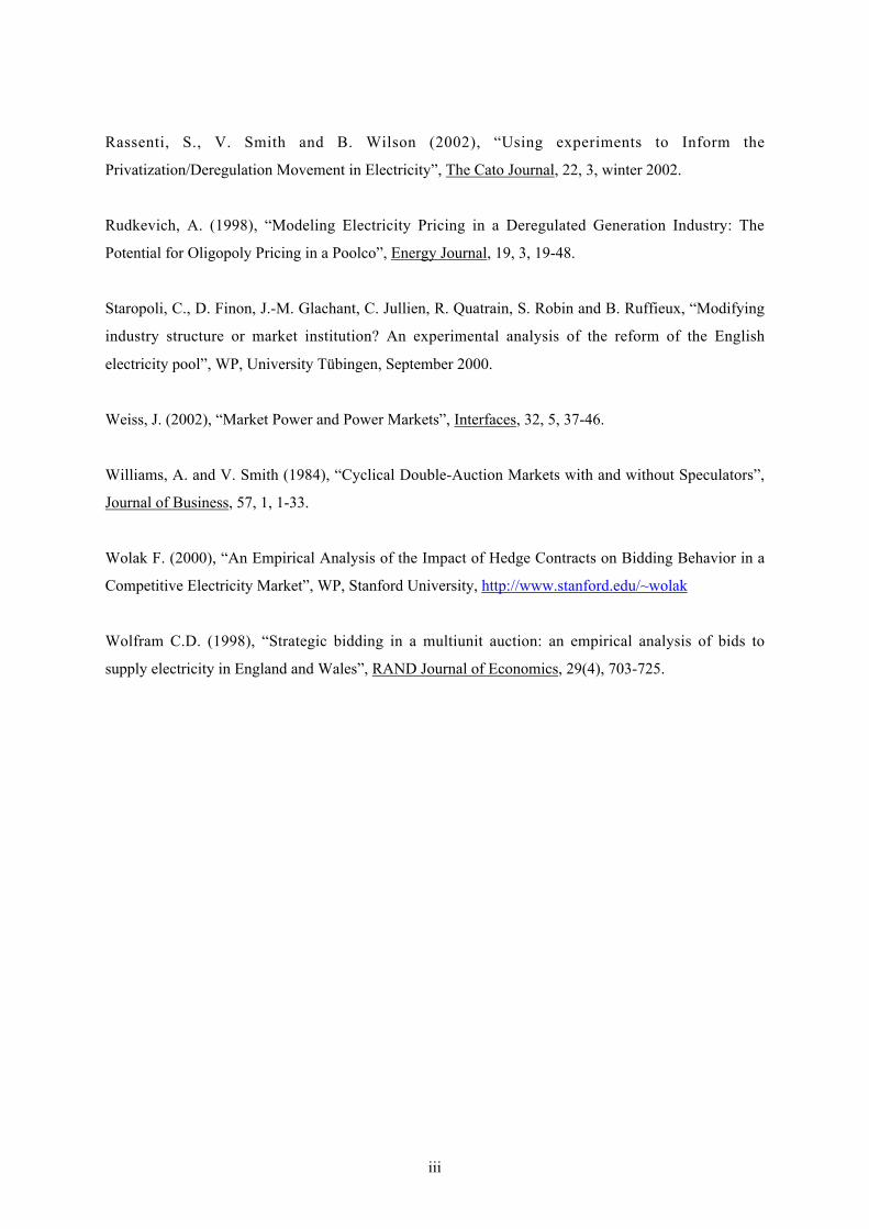
figure 1: Table with the per unit price.

Above, you see an example of the computer screen we will use. The numbers you see will be different in theexperiment. Focus on the 'sharp' picture, in the upper right part.

The table you see in the upper right corner is only an example. Later, you will be able to scroll along the tablewith your mouse, this is not possible in these instructions. You will find a print of the table to be used in theexperiment in an envelop on your desk. This table is the same for everyone. You may open the envelop now.For the time being, only have a look at the table 'Price per Unit'.

There are two columns in the table. The left column (with the heading 'number') gives the total supply (of yourgroup). In the right column (with the heading 'price') you see the price PER UNIT that goes with the numbersupplied. In phase 3, the computer buys all units offered at this price.

If a group (producers plus traders) offers 8 units in phase 3, for example, each participant in that group willreceive 7 francs per unit offered. If you offered 3 of the 8 units, you will get 3x7=21 francs. Note that the priceper unit decreases as the group produces more.

vi

This is the way in which sales in phase 3 take place. Producers also offer units to traders in phase 1. This is whatwe will discuss next.__________

PHASE 1 and PHASE 2

In phase 1, all producers decide how many units they would like to offer to the traders. In this phase, they do notknow which price they will receive per unit. This depends on what traders bid in phase 2. After every producerhas decided how many units to offer to the traders in the group, the total is summed up.

Next, in phase 2, the traders bid a price PER UNIT. The trader with the highest bid receives all units offered atthat price. If neither trader bids a price higher than zero, nothing is sold. If there are bids, then all units areproduced and delivered. The trader then pays each producer for the goods delivered.__________

THE PRODUCERS (SELLERS)

At the beginning of the experiment, each producer will receive 5000 francs as a starting capital. You will seethis amount on your screen (at 'previous earnings') when the experiment starts.

There are costs related to producing goods. These costs are not constant per unit, they are increasing. Thismeans that the costs of the second unit are higher than those of the first unit, etc.

NOTICE: The units in phase 1 and 3 add up. For example, someone who produces 3 units in phase 1 and sellsthem to the traders, starts phase 4 with the fourth unit. This has consequences for production costs.

On the next page, you will see how the costs per unit will appear on your screen.__________

Figure 2: Costs per unit

The table you see above in figure 2 (in the center), is only an example. Later, you will be able to scroll along thetable with your mouse, this is not possible in these instructions. You will also find a print of the table to be usedin the experiment in an envelop on your desk. Have a look at the table 'Costs per Unit’. This table is the samefor everyone.

vii

In the first column, you see the number you produce ('unit'). The second column ('costs') gives the costs of thatunit. You cannot produce a unit without producing the preceding ones. For example, if you want to produce thefifth unit, you must also produce the first, second, third and fourth units. Note that the costs are only determinedby your own production. In no way are your costs affected by what other producers in your group do. Your costsin phase 3 do depend on your own production in phase 1.

To determine the total costs of a certain level of production, you must add up the costs of every unit. To helpyou calculate these total costs, you will find the total costs for the number of units produced under 'cumulative'.__________

Figure 2: Costs per unit

In the table on your screen that gives the costs, you will also be able to indicate your production decision. Thisholds in both phase 1 and phase 3. You do this by clicking one of the numbers under 'sell'. If you click 3, forexample, you indicate that you want to produce and sell 3 units (to be more precise, units 1, 2 and 3). Thesethree units will therefore be marked, if you click on 3.

In phase 3, you will see that the units you sold in phase 1 can no longer be chosen. For example, if you sold 3units to the trader, you can only click on 4, 5, etc.

Each producer can sell (in phase 1 and 3 together) a maximum of 30 units per round.

After you have chosen a number, you need to confirm. This holds in both phase 1 and phase 3. As long as youhave not confirmed, you can still change your decision. Note that you decision is not final until you haveconfirmed it. The experiment will not proceed to the next phase until everyone has confirmed his or herproduction decision. You also need to confirm if you decide to produce zero units.__________

In phase 2, producers do not need to make a decision. They must wait until the traders have decided at whatprice they are willing to buy the goods produced. At the end of phase 2 every producer will receive for everyunit produced the amount determined by the traders.__________

THE TRADERS

At the beginning of the experiment, each trader will receive a starting capital of 45000 francs. In addition, eachtrader will receive 2000 francs in each round. You will see these amounts on your screen when the experimentstarts (at 'previous earnings').

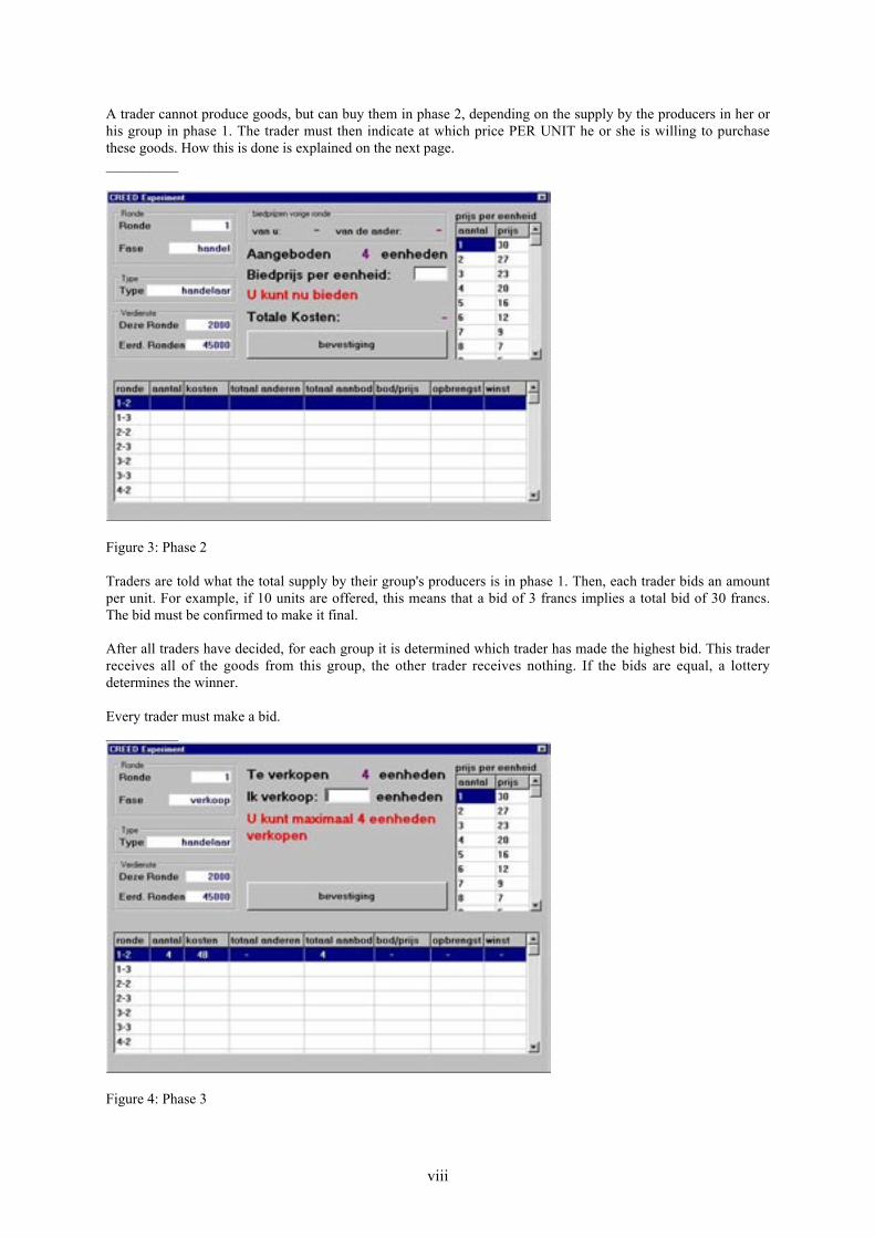
viii

A trader cannot produce goods, but can buy them in phase 2, depending on the supply by the producers in her orhis group in phase 1. The trader must then indicate at which price PER UNIT he or she is willing to purchasethese goods. How this is done is explained on the next page.__________

Figure 3: Phase 2

Traders are told what the total supply by their group's producers is in phase 1. Then, each trader bids an amountper unit. For example, if 10 units are offered, this means that a bid of 3 francs implies a total bid of 30 francs.The bid must be confirmed to make it final.

After all traders have decided, for each group it is determined which trader has made the highest bid. This traderreceives all of the goods from this group, the other trader receives nothing. If the bids are equal, a lotterydetermines the winner.

Every trader must make a bid.__________

Figure 4: Phase 3

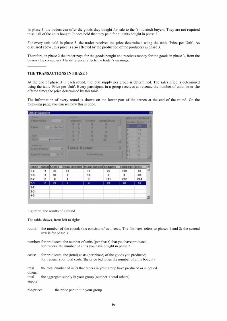
ix

In phase 3, the traders can offer the goods they bought for sale to the (simulated) buyers. They are not requiredto sell all of the units bought. It does hold that they paid for all units bought in phase 2.

For every unit sold in phase 3, the trader receives the price determined using the table 'Price per Unit'. Asdiscussed above, this price is also affected by the production of the producers in phase 3.

Therefore, in phase 2 the trader pays for the goods bought and receives money for the goods in phase 3, from thebuyers (the computer). The difference reflects the trader’s earnings.__________

THE TRANSACTIONS IN PHASE 3

At the end of phase 3 in each round, the total supply per group is determined. The sales price is determinedusing the table 'Price per Unit'. Every participant in a group receives as revenue the number of units he or sheoffered times the price determined by this table.

The information of every round is shown on the lower part of the screen at the end of the round. On thefollowing page, you can see how this is done.__________

Figure 5: The results of a round

The table shows, from left to right:

round: the number of the round; this consists of two rows. The first row refers to phases 1 and 2; the secondrow is for phase 3.

number: for producers: the number of units (per phase) that you have produced;for traders: the number of units you have bought in phase 2.

costs: for producers: the (total) costs (per phase) of the goods you produced;for traders: your total costs (the price bid times the number of units bought).

total the total number of units that others in your group have produced or supplied.others:total the aggregate supply in your group (number + total others)supply:

bid/price: the price per unit in your group

x

revenue: for producers: (per phase) the price per unit times the number of units you produced;for traders: the price per unit times the number of units you supplied in phase 3;

earnings: your profit or loss in the round (revenue - costs).__________

Figure 6: The results thus far

At the end of a round, the profit or loss is added to your earnings thus far. This is shown in the upper left area onyour screen, with the earnings in this round.

You may lose money in a round. If your aggregate earnings should become negative, you will be excluded fromfurther participation in the experiment and you will not be able to produce or trade any more goods. You will gohome without earnings. It is under your own control whether or not you lose money.

You have reached the end of these instructions. You may take your time to go through them again. Please waitquietly until everyone has finished.

xi

Appendix 2

In this appendix, we derive the theoretical predictions given in table 3 of the main text. We do so in

two steps. First, we derive the predictions for a continuous version of the game. Then, we use these as

a double check for the predictions numerically estimated for the case where players can only choose

discrete quantities.

Continuous Case

We extend the duopoly model of Allaz and Vila (1993) to oligopolies with n producers and

(symmetric) quadratic marginal cost functions, M . Total costs are then

. Market demand is known and linear in quantities: with

.

The relation between the forward contract market and the spot market is modeled as a two-stage

game. In the first stage the producing firms take positions in the contract market represented by fi,

i=1,2,..n. In doing so, they take account of the equilibrium prediction that traders will supply to the

spot market everything they obtain on the forward market.23 Hence, in equilibrium, supply to the spot

market is equal to total production.

Producer i’s profit for the second stage, when producing is then given by:

.

which gives the first order conditions:

, (A1)

To determine the equilibrium quantities to be produced in stage 2, we solve the system of

equations (A1) in terms of producers’ forward market positions . The solution to (A1) has

no analytical expression and is numerically determined. It has 8 roots, but only one of them,

, leads to three non-negative forward positions. These quantities (as functions of )

determine the equilibrium price .

xii

Moving to stage 1, we proceed with determining (numerically) the quantities supplied to the forward

market. At stage 1, producers know that (in equilibrium) traders will bid the (spot) market equilibrium

price for the units on the forward market. The producers’ profit (as a function of forward positions

and anticipated stage 2 reactions) is then given by:

,

where F-i denotes the aggregated forward positions of the other producers. Taking the first order

conditions and solving for fi, we derive the producers’ equilibrium forward

positions , which are used to determine the equilibrium spot market production levels

and the market price .

If there is no forward contract market, then fi = 0 and (A1) boils down to the standard

Cournot profit maximization program. Table A reports the numerically determined Nash equilibria for

C3.0, C3.2, C4.0 as well as the joint profit maximizing (JPM) and Walras (W) scenarios with 3 and 4

producers.24 The JPM and W cases are determined in the standard way. To be complete, we need to

double check that offering all units for sale on the spot market is a best response for traders (as

assumed above). It turns out that the best reply is to sell 17.2 units, which is more than the 11.4 units

they have. Hence, the corner solution of reselling everything is indeed a best response.

Table A: Benchmarks for the Continuous Casea

JPM(n=3)

JPM(n=4)

NEC3.0

NEC3.2

NEC4.0

Walras(n=3)

Walras(n=4)

--- --- --- 5.736 --- --- ---

10.777 8.509 14.406 15.320 12.364 17.071 14.406

32.330 34.034 43.217 45.959 49.457 51.212 57.623

1127.08 1081.07 833.143 759.112 664.652 617.283 444.190

Prod.S. 33576.5 34850.0 29389.9 26977.7 27203.4 20772.0 16774.1

Cons.S. 14110.8 15637.6 25214.0 28514.9 33021.3 35405.6 44824.9

TotalS. 47687.3 50488.1 54603.9 55492.6 60224.7 56177.6 61599.0

Eff. (%) 84.9 82.0 97.2 98.8 97.8 100 100

a = forward production by producer i ; = total quantity produced by producer i; = total

quantity produced in the market; = transaction price; prosur=producer surplus (trader surplus is equal

to 0); consur= consumer surplus; surplus=total surplus; eff = efficiency.

23 We will return to this assumption, below.24 It may seem surprising that in C3.2 only somewhat more than a third is sold on the forward market, whereas with constantmarginal costs this quantity would be close to 50%. Intuitively, the fact that marginal costs are increasing intensifies thedilemma character of participation in the forward market and, hence, leads firms to limit their sales in that sub-market.

xiii

Discrete Case

As subjects in our experiment could only supply integer quantities, we base our data analysis on the

equilibrium outcomes for the discrete case. This is determined using the GAMBIT software

(McKelvey, McLennan and Turocy, 2002). 25

We start with the cases without a forward market (C3.0 and C4.0). Given the large strategy

sets (i.e., 30 possible actions per producer), which would require a considerable time and computing

facilities to explore all possibilities, we searched for equilibria in windows of 20 units (i.e., for

, , , etc. Using this method, we found equilibria in pure

strategies. In C3.0, the equilibria entail any two producers supplying 14 units and the third producer

supplying 15 units. In aggregate they produce 43 units equilibrium (compare this to the equilibrium

production of 43.217 units in the continuous case; cf. table A). In C4.0, three producers supply 12

units in equilibrium and the fourth supplies 13 units, for a total of 49 (49.457 in the continuous case).

These numbers are reported in table 3 of the main text.

For C3.2, we restrict the window size for the equilibrium search in GAMBIT to 4 units for the

forward market and 5 units for the spot market (e.g., we search for and ,

and , etc.). In addition, we reduced the two-stage game to its normal form

and searched for an equilibrium of the type ( , ) in pure and mixed strategies. The

equilibrium that we found when quantities are discrete is partially in mixed strategies: each producer

supplies six units on the forward market. On the spot market, each producer supplies 9 units with

probability .944343 or 10 units with probability .055657. This yields a total (expected) supply of

45.167. This is slightly lower than the equilibrium quantity for the continuous case (45.959).

25 The JPM and W predictions for the discrete case are determined in a straightforward manner.