Electricity market operations under increasing uncertainty
213
POUR L'OBTENTION DU GRADE DE DOCTEUR ÈS SCIENCES acceptée sur proposition du jury: Prof. A. Skrivervik, présidente du jury Dr S.-R. Cherkaoui, Prof. A. J. Conejo, directeurs de thèse Prof. A. Bakirtzis, rapporteur Prof. T. Gomez, rapporteur Prof. J.-Y. Le boudec, rapporteur Electricity market operations under increasing uncertainty THÈSE N O 7894 (2017) ÉCOLE POLYTECHNIQUE FÉDÉRALE DE LAUSANNE PRÉSENTÉE LE 25 AOÛT 2017 À LA FACULTÉ DES SCIENCES ET TECHNIQUES DE L'INGÉNIEUR GROUPE SCI STI RC PROGRAMME DOCTORAL EN GÉNIE ÉLECTRIQUE Suisse 2017 PAR Farzaneh ABBASPOURTORBATI
-
Upload
khangminh22 -
Category
Documents
-
view
3 -
download
0
Transcript of Electricity market operations under increasing uncertainty

POUR L'OBTENTION DU GRADE DE DOCTEUR ÈS SCIENCES
acceptée sur proposition du jury:
Prof. A. Skrivervik, présidente du juryDr S.-R. Cherkaoui, Prof. A. J. Conejo, directeurs de thèse
Prof. A. Bakirtzis, rapporteurProf. T. Gomez, rapporteur
Prof. J.-Y. Le boudec, rapporteur
Electricity market operations under increasing uncertainty
THÈSE NO 7894 (2017)
ÉCOLE POLYTECHNIQUE FÉDÉRALE DE LAUSANNE
PRÉSENTÉE LE 25 AOÛT 2017 À LA FACULTÉ DES SCIENCES ET TECHNIQUES DE L'INGÉNIEUR
GROUPE SCI STI RCPROGRAMME DOCTORAL EN GÉNIE ÉLECTRIQUE
Suisse2017
PAR
Farzaneh ABBASPOURTORBATI


You are educated when you have the ability to listen to
almost anything without losing your temper or self-confidence.
–– Robert Frost
Dedicated to my beloved family.


Abstract
Decision making in electricity markets under uncertainty has worldwide gained attention due
to an increasing number of uncertain parameters associated to technology developments and
market evolution. Hence, the market operator faces new challenges pertaining to technical
and economic aspects of electricity markets. To tackle these challenges, appropriate models
are necessary.
This dissertation aims to analyze some of the challenges pertaining to the management in
electricity markets under uncertainty and to provide the market operator with the models that
enable it to make informed decisions in such uncertain market environments.
In the context above, we categorize market operation problems into the following four groups.
With the aim of obtaining informed day-ahead decisions in the presence of a number of intra-
day markets and high renewable production, we propose a multi-stage stochastic clearing
model, where the first stage represents the day-ahead market, n stages model n intra-day
markets, and a final stage represents real-time operation. The proposed multi-stage clearing
model considers not only different realizations of renewable power output, but also how these
realizations evolve from day-ahead forecasts into real-time values, and allows flexibility for
the contribution of renewable production in both the day-ahead and intra-day markets in
form of scheduled productions and their adjustments. This improves the market outcomes
and integration of renewable generation.
With the purpose of obtaining marginal prices with cost-recovery features, we develop novel
pricing methodologies in the presence of non-convexities and uncertainty in the market.
These models minimize the duality gap of a stochastic non-convex clearing model and the
dual problem of a relaxed version of this original model subject to primal constraints, dual
constraints, cost-recovery constraints, and integrity constraints. The prices obtained deviate
in the least possible manner from conventional marginal prices. This implies that a minimum
deviation from the optimal value of social welfare is also guaranteed. Moreover, the new
prices preserve the short-term economic efficiency and long-term cost recovery properties of
iii

marginal prices, while eliminating a need for uplifts.
We provide insightful analyses on the impact of demand flexibility on the operational and eco-
nomic aspects of the power system operation. We investigate how market prices are affected
by flexible demands and what economic consequences are observed. For this purpose, we
consider a system with high renewable production and a number of comparatively expensive
fast-ramping units, which are flexible to react to the uncertainty pertaining to renewable
power production. We investigate the role of flexible demands from an economic viewpoint,
particularly the impact of flexible demands on demand revenues.
Lastly, we develop a risk-neutral two-stage stochastic clearing model and a risk-averse one
for reserve markets. We particularly focus on the Swiss reserve market, which consists of a
weekly market with a gate closure one week ahead of real-time operation and a daily market
with a gate closure two days ahead of real time. The decision-making problem consists of
determining which amount of reserves to procure in the weekly market and which one in the
daily market. In the proposed two-stage model, the first stage represents the weekly market
and the second stage the daily market. The source of uncertainty is the unknown offers in the
daily market, which are represented by scenarios. If the system operator aims to minimize the
risk pertaining to expensive reserve offers in the daily market, a risk-averse instance of this
two-stage clearing model is also proposed.
Key words: Electricity Markets, Multi-Stage Stochastic Programming, Uncertainty Man-
agement, Decision Making, Pricing Schemes, Flexible Demands, Reserve Markets, Renew-
able Production, Intra-Day Markets, Risk, Non-convexity, Uplift, Cost recovery, Value of
the Stochastic Solution, Informed Day-ahead Decisions.
iv

Résumé
La prise de décision dans les marchés de l’électricité sujet à l’incertitude attire l’attention
à l’échelle mondiale en raison du nombre croissant de paramètres incertains associés aux
développements technologiques et à l’évolution du marché. Par conséquent, l’opérateur du
marché doit faire face à de nouveaux défis liés aux aspects techniques et économiques des
marchés de l’électricité. Pour relever ces défis, des modèles appropriés sont nécessaires.
Cette thèse vise à analyser un certain nombre de défis liés à la gestion des marchés de l’élec-
tricité sujet à l’incertitude et à fournir à l’opérateur du marché des modèles permettant de
prendre des décisions appropriées dans des environnements de marché aussi incertains. Aussi,
dans le contexte ci-dessus, nous classons les problèmes de fonctionnement du marché dans
les quatre groupes suivants.
Dans le but d’obtenir des décisions le jour d’avant en présence d’un certain nombre de
marchés intra-journaliers et d’une production renouvelable élevée, nous proposons un modèle
de marché stochastique à plusieurs étapes, où les étapes représentent respectivement le
marché du jour d’avant, N marchés intra journaliers, et un marché en temps réel. Le modèle
multi-étapes proposé considère non seulement les différentes réalisations de la production
d’énergie renouvelable, mais aussi la façon dont ces réalisations évoluent depuis leur prévision
le jour d’avant jusqu’à leur valeur en temps réel. Il permet une flexibilité de la production
d’énergie renouvelable dans le marché du jour d’avant et les marchés intra journaliers sous
forme de productions programmées et d’ajustement. Cela améliore les résultats du marché
ainsi que l’intégration de la production renouvelable.
Dans le but d’obtenir des prix marginaux avec des options de recouvrement des coûts, nous
développons un nouveau mécanisme de tarification tenant compte de la présence de non-
convexité et d’incertitude dans le modèle de marché. Ce modèle minimise l’écart de dualité
entre un modèle de marché stochastique non convexe et sa version duale relaxée tout en tenant
compte des contraintes du problème primal, des contraintes duals, des contraintes concernant
le recouvrement des coûts et des contraintes sur les variables binaires. Les prix obtenus
v

s’écartent le moins possible des prix marginaux conventionnels. En outre, Ces nouveaux prix
préservent l’efficacité économique à court terme et les propriétés de recouvrement des coûts
à long terme des prix marginaux tout en éliminant la nécessité des up-lifts.
Ensuite, nous fournissons des analyses approfondies sur l’impact de la flexibilité de la de-
mande sur les aspects opérationnels et économiques de l’exploitation du réseau électrique.
Nous étudions comment les prix du marché sont affectés par des demandes flexibles et les
conséquences économiques observées. À cet effet, nous considérons un système à forte pro-
duction renouvelable et un certain nombre d’unités à forte montée en charge et réputées
onéreuses. Ces dernières sont considérées suffisamment flexibles pour réagir à l’incertitude
relative à la production d’énergie renouvelable. Nous étudions le rôle des demandes flexibles
d’un point de vue économique, en particulier l’impact des demandes flexibles sur les revenus
de la demande.
Enfin, pour les marchés de réserve, nous développons deux modèles stochastiques à deux
étapes respectivement neutre vis-à-vis du risque et robuste face au risque. Nous nous concen-
trons particulièrement sur le marché de réserve suisse qui comprend un marché hebdoma-
daire avec clôture une semaine avant l’exploitation en temps réel et un marché quotidien
avec clôture deux jours avant le temps réel. Le problème de la prise de décision consiste à
déterminer les quantités de réserve à vendre sur le marché hebdomadaire et le marché journa-
lier respectivement. Dans le modèle proposé en deux étapes, la première étape représente
le marché hebdomadaire et la deuxième étape représente le marché journalier. La source
d’incertitude est liée à l’offre inconnue sur le marché quotidien qui est représentée par des
scénarios. Si l’opérateur du système vise à minimiser le risque lié aux prix des offres de réserve
sur le marché quotidien, le modèle de marché robuste face au risque est proposée à cet égard.
Mots clefs : Marchés d’électricité, Programmation stochastique à multi-étapes, Gestion de
l’incertitude, Prise de décision, Mécanisme de fixation des prix, Demandes flexibles, Mar-
ché de réserve, Production renouvelable, Marchés intra journaliers, Risque, Non convexité,
Uplift, Recouvrement des coûts, Valeur de la solution stochastique.
vi

Acknowledgements
This thesis summarizes the work done over the course of four years at the Power Systems
Group (PWRS) at EPFL. During my PhD, I was also working at the TSO Market Development
team at Swissgrid. It has been a wonderful time and unique opportunity for me. I would like
to extend my sincere gratitude to everyone I have interacted with, both on a professional and
a personal level.
First and foremost, I would like to express my deepest gratitude to my advisors, Dr. Rachid
Cherkaoui and Prof. Antonio Conejo, for invaluable help and support. Rachid, thank you
for giving me such a wonderful opportunity at EPFL, providing me with flexibility and being
patient with me. Thank you for detailed discussions. Antonio, thank you for supporting me
with your vast knowledge and patience, and for hosting me at The Ohio State University, which
was a turning point in my research. I am grateful to be your 20th graduated PhD student! And
also, thank you for writing so many good books! I had been trained by your books years before
I had the chance to collaborate with you.
My special thanks go to Dr. Marek Zima, leader of the TSO Market Development team at
Swissgrid. Marek, thank you for the courage you gave me to go through this path, and for
advising me on my first research work Combined Auction when I was just a newbie. The
outcome of your idea in this project reported in Chapter 5 of this thesis. Thank you for your
support and flexibility over all these years.
Pursuing a PhD at EPFL in Lausanne and a full-time job at Swissgrid in Laufenburg, while
living in Zurich was only possible with the flexibility and support that Rachid, Antonio, and
Marek provided me. Thank you very much.
I would also like to express my gratitude to the committee members for valuable comments
and discussions during and after the PhD exam. Respecting travel distance (!), my sincere
thanks goes to Prof. Tomas Gomez. It was a great pleasure to get to know you and to have your
opinion on my work. Thank you for insightful comments. I would like to thank the committee
member Prof. Anastasios Bakirtzis. It was always a great pleasure for me to have a discussion
vii

Acknowledgements
with you in different conferences. Thank you for constructive comments on my thesis. I would
also like to express my gratitude to the committee member Prof. Jean-Yve Le boudec. Thank
you for your valuable comments, and careful correction regarding my inaccurate statement
on marginal pricing!
It was an incredible luck for me to get to know Prof. Daniel Kuhn. He is a wonderful teacher.
I regret that I could not take more courses with him. Should the fundamental knowledge of
optimization be a dream, as perhaps the ball in Royal Palace to Cinderella, then I would be
confident to nominate Daniel as the fairy Godfather whose magic spell would never wear off! I
have learnt a lot from him in convex optimization course.
I would like to express my gratitude to Prof. Göran Andersson, who was also my master thesis
advisor, for kindly providing me access to servers in the Power System Laboratory (PSL) at
ETH Zurich. This helped me progressing with the work reported in Chapter 3 of this thesis.
I would like to thank Dr. Mokhtar Bozorg and Dr. Mostafa Nick at the Distributed Electrical
Systems Laboratory (DESL) at EPFL for their great unconditional help over all these years
ranging from administrative issues to detailed technical discussions. I really appreciate your
time to listen to my last minute PhD defense rehearsal.
I would like to extend my appreciation to to-be-soon Dr. Stavros Karagiannopoulos and to
to-be-soon Prof. Line Roald at the PSL for their computational support and fruitful discussions
and collaborations we had in different occasions.
I would like to extend my thanks to my colleagues at Swissgrid and all members of DESL and
PWRS for the great time we had together.
Throughout these years, I have been fortunate to work with a number of students. I would like
to thank Athanasios Troupakis, Anneta Matenli, Georgios Chatzis, and Haoyuan Qu for their
contributions and for choosing to work with me. I would also like to thank my collaborators
who co-supervised these projects.
At this point, I would like to thank Dr. Robin Vujanic and to-be-soon Dr. Tobias Sutter for
warmly welcoming me in their office over all evenings and weekends at Automatic Control
Laboratory (IfA) at ETH Zurich. I am sure that I am a better officemate than Peyman, at least I
am more quiet than him!
At a personal level, I want to thank my terrific friends who made my Zurich life memorable, as
well as my stays in Boston! Thank you for sharing fun times, brunches, game nights, hikes, but
also for standing by me in my difficult moments.
viii

Acknowledgements
I am greatly indebted to my dear parents, my father, Reza, who taught me being a woman is no
excuse for not reaching far, and my mother, Esmat, for encouraging me to explore the world.
Thanks to my two wonderful sisters for their unconditional love and empathy. Without them,
I would never have been where I am today.
Last, I want to thank my best friend, my discussion partner, and my soulmate, Peyman. When
spending all those weekends, evenings, and holidays on my research, you always supported
me with compassion and encouragement. Peyman, it has been a long path with many ups
and downs. Had I have another chance with you, I would definitely have held your hand more
strongly. I can also keep it simple: I love you, too.
Farzaneh Abbaspourtorbati
July 2017
Zurich, Switzerland
ix


Contents
Abstract (English/Français/Deutsch) iii
Acknowledgements vii
Contents xi
List of figures xvii
List of tables xxi
Notations xxv
List of Symbols Used in Chapters 2, 3, and 4 . . . . . . . . . . . . . . . . . . . . . . . . xxv
List of Symbols Used in Chapter 5 . . . . . . . . . . . . . . . . . . . . . . . . . . . . . . xxviii
1 Introduction 1
1.1 Motivation . . . . . . . . . . . . . . . . . . . . . . . . . . . . . . . . . . . . . . . . . 1
1.2 Market Operations . . . . . . . . . . . . . . . . . . . . . . . . . . . . . . . . . . . . 4
1.3 Literature Review . . . . . . . . . . . . . . . . . . . . . . . . . . . . . . . . . . . . . 5
1.3.1 Methodology: Stochastic programming . . . . . . . . . . . . . . . . . . . . 5
1.3.2 Market Operations: Scheduling of Energy and Reserves . . . . . . . . . . 6
1.3.3 Market Operations: Pricing . . . . . . . . . . . . . . . . . . . . . . . . . . . 7
1.3.4 Market Operations: Demand Flexibility . . . . . . . . . . . . . . . . . . . . 8
xi

Contents
1.4 Market Operations & Uncertainty Management . . . . . . . . . . . . . . . . . . . 9
1.5 Thesis Objectives . . . . . . . . . . . . . . . . . . . . . . . . . . . . . . . . . . . . . 11
1.5.1 Objectives for the Multi-Stage Market-Clearing Model . . . . . . . . . . . 11
1.5.2 Objectives for the Pricing Scheme Pertaining to a Stochastic Non-Convex
Market-Clearing Model . . . . . . . . . . . . . . . . . . . . . . . . . . . . . 11
1.5.3 Objectives for the Economic Impact of Flexible Demands . . . . . . . . . 12
1.5.4 Objectives for Stochastic Reserve Clearing Model . . . . . . . . . . . . . . 12
1.6 Thesis Outline . . . . . . . . . . . . . . . . . . . . . . . . . . . . . . . . . . . . . . . 12
2 Multi-Stage Stochastic Market-Clearing Model 15
2.1 Introduction . . . . . . . . . . . . . . . . . . . . . . . . . . . . . . . . . . . . . . . . 15
2.2 Decision-Making Process and Scenario Tree . . . . . . . . . . . . . . . . . . . . . 17
2.3 Assumptions . . . . . . . . . . . . . . . . . . . . . . . . . . . . . . . . . . . . . . . . 19
2.4 Model Description . . . . . . . . . . . . . . . . . . . . . . . . . . . . . . . . . . . . 20
2.4.1 Three-stage Stochastic Clearing Model . . . . . . . . . . . . . . . . . . . . 20
2.4.2 Two-stage Stochastic Clearing Model . . . . . . . . . . . . . . . . . . . . . 31
2.4.3 Metrics for Performance Evaluation . . . . . . . . . . . . . . . . . . . . . . 35
2.4.4 Economic Aspect: Pricing Scheme, Cost-Recovery Conditions & Notion
of Uplift . . . . . . . . . . . . . . . . . . . . . . . . . . . . . . . . . . . . . . . 36
2.5 Illustrative Example . . . . . . . . . . . . . . . . . . . . . . . . . . . . . . . . . . . . 38
2.5.1 Data . . . . . . . . . . . . . . . . . . . . . . . . . . . . . . . . . . . . . . . . . 38
2.5.2 Outcomes of the Three-Stage Model . . . . . . . . . . . . . . . . . . . . . . 39
2.5.3 Performance of the Three-Stage Model vs. the Two-Stage One . . . . . . 42
2.6 Case Studies . . . . . . . . . . . . . . . . . . . . . . . . . . . . . . . . . . . . . . . . 45
2.6.1 Data . . . . . . . . . . . . . . . . . . . . . . . . . . . . . . . . . . . . . . . . . 45
2.6.2 Scenarios . . . . . . . . . . . . . . . . . . . . . . . . . . . . . . . . . . . . . . 46
xii

Contents
2.6.3 Base Case . . . . . . . . . . . . . . . . . . . . . . . . . . . . . . . . . . . . . 47
2.6.4 Analyses of Flexibility of Units for Reserve Provision and Different Adjust-
ment Bounds . . . . . . . . . . . . . . . . . . . . . . . . . . . . . . . . . . . 49
2.6.5 Computation Time . . . . . . . . . . . . . . . . . . . . . . . . . . . . . . . . 54
2.6.6 Case Study Conclusion . . . . . . . . . . . . . . . . . . . . . . . . . . . . . . 56
2.7 Summary and Conclusion of the Chapter . . . . . . . . . . . . . . . . . . . . . . . 57
3 Pricing Schemes Pertaining to A Stochastic Non-Convex Market-Clearing Model 59
3.1 Introduction . . . . . . . . . . . . . . . . . . . . . . . . . . . . . . . . . . . . . . . . 59
3.2 A New Pricing Mechanism with Cost Recovery . . . . . . . . . . . . . . . . . . . . 61
3.3 Assumptions . . . . . . . . . . . . . . . . . . . . . . . . . . . . . . . . . . . . . . . . 63
3.4 Decision-Making Process . . . . . . . . . . . . . . . . . . . . . . . . . . . . . . . . 64
3.5 Model Description . . . . . . . . . . . . . . . . . . . . . . . . . . . . . . . . . . . . 65
3.5.1 Primal Problem: Two-Stage Clearing Model . . . . . . . . . . . . . . . . . 65
3.5.2 Dual Problem of Two-stage Clearing Model . . . . . . . . . . . . . . . . . 67
3.5.3 Primal-Dual Problem . . . . . . . . . . . . . . . . . . . . . . . . . . . . . . . 69
3.5.4 Cost Recovery Conditions . . . . . . . . . . . . . . . . . . . . . . . . . . . . 73
3.5.5 Linearization of Cost-Recovery Conditions . . . . . . . . . . . . . . . . . . 74
3.5.6 Complete Model . . . . . . . . . . . . . . . . . . . . . . . . . . . . . . . . . 77
3.6 Illustrative Example . . . . . . . . . . . . . . . . . . . . . . . . . . . . . . . . . . . . 77
3.6.1 Data . . . . . . . . . . . . . . . . . . . . . . . . . . . . . . . . . . . . . . . . . 77
3.6.2 Market Outcomes . . . . . . . . . . . . . . . . . . . . . . . . . . . . . . . . . 79
3.7 Case Studies . . . . . . . . . . . . . . . . . . . . . . . . . . . . . . . . . . . . . . . . 82
3.7.1 Data . . . . . . . . . . . . . . . . . . . . . . . . . . . . . . . . . . . . . . . . . 83
3.7.2 Case I: No Network Congestion . . . . . . . . . . . . . . . . . . . . . . . . . 84
3.7.3 Impact of Minimum Up/Down Time Constraints . . . . . . . . . . . . . . 87
xiii

Contents
3.7.4 Case II: Network Congestion . . . . . . . . . . . . . . . . . . . . . . . . . . 89
3.7.5 Discussion on Social Welfare Gap and Computation Time . . . . . . . . . 90
3.7.6 Impact of Linearization Step . . . . . . . . . . . . . . . . . . . . . . . . . . 92
3.7.7 Case Study Conclusion . . . . . . . . . . . . . . . . . . . . . . . . . . . . . . 93
3.8 Summary and Conclusion of the Chapter . . . . . . . . . . . . . . . . . . . . . . . 94
4 Economic Impact of Flexible Demands 95
4.1 Introduction . . . . . . . . . . . . . . . . . . . . . . . . . . . . . . . . . . . . . . . . 95
4.2 Approach . . . . . . . . . . . . . . . . . . . . . . . . . . . . . . . . . . . . . . . . . . 96
4.3 Assumptions . . . . . . . . . . . . . . . . . . . . . . . . . . . . . . . . . . . . . . . . 97
4.4 Model Description: Two-Stage Stochastic Clearing with Flexible Demands . . . 98
4.4.1 Flexible Demands as Decision Variables . . . . . . . . . . . . . . . . . . . 98
4.4.2 Constraints pertinent to Demand Flexibility . . . . . . . . . . . . . . . . . 100
4.4.3 Mathematical Model . . . . . . . . . . . . . . . . . . . . . . . . . . . . . . . 101
4.5 Illustrative Example . . . . . . . . . . . . . . . . . . . . . . . . . . . . . . . . . . . . 104
4.5.1 Data . . . . . . . . . . . . . . . . . . . . . . . . . . . . . . . . . . . . . . . . . 104
4.5.2 Market Outcomes . . . . . . . . . . . . . . . . . . . . . . . . . . . . . . . . . 106
4.6 Case Studies . . . . . . . . . . . . . . . . . . . . . . . . . . . . . . . . . . . . . . . . 108
4.6.1 Data . . . . . . . . . . . . . . . . . . . . . . . . . . . . . . . . . . . . . . . . . 109
4.6.2 Base Case: No Congestion . . . . . . . . . . . . . . . . . . . . . . . . . . . . 110
4.6.3 Impact of Ramping Limits and Congestion . . . . . . . . . . . . . . . . . . 113
4.6.4 Case Study Conclusions . . . . . . . . . . . . . . . . . . . . . . . . . . . . . 116
4.7 Summary and Conclusion of the Chapter . . . . . . . . . . . . . . . . . . . . . . . 117
5 Two-Stage Stochastic Clearing Model for the Reserve Market 119
5.1 Introduction . . . . . . . . . . . . . . . . . . . . . . . . . . . . . . . . . . . . . . . . 119
xiv

Contents
5.2 The Swiss Reserve Market . . . . . . . . . . . . . . . . . . . . . . . . . . . . . . . . 120
5.2.1 Technical Description of Reserves in Europe . . . . . . . . . . . . . . . . . 120
5.2.2 Reserve Dimensioning Criteria . . . . . . . . . . . . . . . . . . . . . . . . . 122
5.2.3 Structure of the Swiss Reserve Market . . . . . . . . . . . . . . . . . . . . . 127
5.2.4 Drawbacks of the Common Practice . . . . . . . . . . . . . . . . . . . . . . 129
5.3 Decision-Making Process . . . . . . . . . . . . . . . . . . . . . . . . . . . . . . . . 130
5.4 Scenarios Modeling Reserve Offers in Daily Market . . . . . . . . . . . . . . . . . 130
5.5 Practical Aspects . . . . . . . . . . . . . . . . . . . . . . . . . . . . . . . . . . . . . 132
5.6 Model Description . . . . . . . . . . . . . . . . . . . . . . . . . . . . . . . . . . . . 132
5.6.1 Risk-Neutral Model . . . . . . . . . . . . . . . . . . . . . . . . . . . . . . . . 133
5.6.2 Risk-Averse Model . . . . . . . . . . . . . . . . . . . . . . . . . . . . . . . . 140
5.6.3 The Reference Model (Common Practice) . . . . . . . . . . . . . . . . . . 142
5.6.4 Metrics: Perfect Information Model & Actual Cost . . . . . . . . . . . . . . 144
5.7 Case Studies . . . . . . . . . . . . . . . . . . . . . . . . . . . . . . . . . . . . . . . . 147
5.7.1 Outcomes of the Risk-Neutral Model . . . . . . . . . . . . . . . . . . . . . 148
5.7.2 Discussion on the Number of Scenarios, Optimal Expected Reserve Cost
and Computation Time . . . . . . . . . . . . . . . . . . . . . . . . . . . . . 152
5.7.3 Simulation Results for the Risk-Averse Model . . . . . . . . . . . . . . . . 153
5.7.4 Case Study Conclusions . . . . . . . . . . . . . . . . . . . . . . . . . . . . . 157
5.8 Summary and Conclusion of the Chapter . . . . . . . . . . . . . . . . . . . . . . . 157
6 Closure 159
6.1 Summary and Conclusions . . . . . . . . . . . . . . . . . . . . . . . . . . . . . . . 159
6.1.1 Multi-Stage Stochastic Clearing Model . . . . . . . . . . . . . . . . . . . . 159
6.1.2 Pricing Scheme Pertaining to A Stochastic Non-Convex Market-Clearing
Model . . . . . . . . . . . . . . . . . . . . . . . . . . . . . . . . . . . . . . . . 160
xv

Contents
6.1.3 Economic Impact of Flexible Demands . . . . . . . . . . . . . . . . . . . . 161
6.1.4 Stochastic Clearing model for the Reserve Market . . . . . . . . . . . . . . 162
6.2 Contributions . . . . . . . . . . . . . . . . . . . . . . . . . . . . . . . . . . . . . . . 163
6.3 Future Research Work . . . . . . . . . . . . . . . . . . . . . . . . . . . . . . . . . . 164
Appendices 165
A Some Notions on Multi-Stage Stochastic Programming . . . . . . . . . . . . . . . 165
A.1 Mathematical Description of Multi-Stage Stochastic Programming . . . 165
A.2 Value of the Stochastic Solution for Multi-Stage Stochastic Programming 166
B IEEE 24-Node System Data . . . . . . . . . . . . . . . . . . . . . . . . . . . . . . . 167
C Minimum Up- and Down-Time Constraints . . . . . . . . . . . . . . . . . . . . . 169
Bibliography 171
Curriculum Vitae 177
List of Publications 179
xvi

List of Figures
2.1 Scenario tree for a multi-stage decision-making process . . . . . . . . . . . . . . 17
2.2 Scenario trees for the three-stage market-clearing model and its two-stage coun-
terpart . . . . . . . . . . . . . . . . . . . . . . . . . . . . . . . . . . . . . . . . . . . 18
2.3 Scenario tree and scenario paths (dashed lines) for a three-stage market-clearing
model . . . . . . . . . . . . . . . . . . . . . . . . . . . . . . . . . . . . . . . . . . . . 19
2.4 Test system . . . . . . . . . . . . . . . . . . . . . . . . . . . . . . . . . . . . . . . . . 38
2.5 Scheduled power productions, power adjustments, and deployed reserves in
period t1 . . . . . . . . . . . . . . . . . . . . . . . . . . . . . . . . . . . . . . . . . . 40
2.6 Scheduled power productions, power adjustments, and deployed reserves in
period t2 . . . . . . . . . . . . . . . . . . . . . . . . . . . . . . . . . . . . . . . . . . 40
2.7 Scheduled productions and deployed reserves result from two-stage model in
period t1. . . . . . . . . . . . . . . . . . . . . . . . . . . . . . . . . . . . . . . . . . . 43
2.8 Scheduled productions and deployed reserves result from two-stage model in
period t2. . . . . . . . . . . . . . . . . . . . . . . . . . . . . . . . . . . . . . . . . . . 44
2.9 Scenario tree for the three stages of day-ahead market, intra-day market, and
real-time operation. Each scenario involves 24 values for the wind power output
of wind unit. . . . . . . . . . . . . . . . . . . . . . . . . . . . . . . . . . . . . . . . . 47
2.10 Day-ahead clearing prices from the three-stage model and the two-stage model
over all periods. . . . . . . . . . . . . . . . . . . . . . . . . . . . . . . . . . . . . . . 49
2.11 Expected profit, expected cost, consumer payment, and uplift for different cases. 51
2.12 Day-ahead clearing prices for different cases . . . . . . . . . . . . . . . . . . . . . 51
xvii
List of Figures
2.13 Different load profiles . . . . . . . . . . . . . . . . . . . . . . . . . . . . . . . . . . 52
2.14 Expected costs for different load profiles and different limited cases . . . . . . . 52
3.1 Test system . . . . . . . . . . . . . . . . . . . . . . . . . . . . . . . . . . . . . . . . . 78
3.2 Scheduled productions and deployed reserves obtained from the conventional
method and the proposed pricing approaches. . . . . . . . . . . . . . . . . . . . 79
3.3 Day-ahead profit and expected profit . . . . . . . . . . . . . . . . . . . . . . . . . 81
3.4 Day-ahead Profit (RTS no congestion case). . . . . . . . . . . . . . . . . . . . . . 84
3.5 Day-ahead prices at node 2 under different approaches (RTS no congestion case). 85
3.6 Expected Profit (RTS no congestion case). . . . . . . . . . . . . . . . . . . . . . . . 86
3.7 LMPs at t18 (up) and t21 (down) obtained by the different approaches. . . . . . . 89
3.8 Cost increase in percent, and consumer payment increase in percent for different
load profiles (RTS no congested case) . . . . . . . . . . . . . . . . . . . . . . . . . 90
3.9 Cost increase in percent, and consumer payment increase in percent for different
load profiles (RTS congestion case) . . . . . . . . . . . . . . . . . . . . . . . . . . 91
3.10 Social welfare gaps as a percentage of the optimal expected cost obtained from
primal problem 3.4 for different load profiles . . . . . . . . . . . . . . . . . . . . . 91
4.1 Test system . . . . . . . . . . . . . . . . . . . . . . . . . . . . . . . . . . . . . . . . . 105
4.2 Day-ahead scheduled units and demands - illustrative example . . . . . . . . . 106
4.3 Day-ahead production scheduled over 24 periods (RTS system) . . . . . . . . . . 110
4.4 Demand pattern obtained from the flexible and inflexible demand cases (RTS
system) . . . . . . . . . . . . . . . . . . . . . . . . . . . . . . . . . . . . . . . . . . . 111
4.5 Day-ahead prices obtained from the flexible and inflexible demand cases (RTS
system) . . . . . . . . . . . . . . . . . . . . . . . . . . . . . . . . . . . . . . . . . . . 112
4.6 The day-ahead prices at node 5 over different periods (ramping limits and con-
gestion case) . . . . . . . . . . . . . . . . . . . . . . . . . . . . . . . . . . . . . . . . 114
4.7 RTS case study with congestion: nodal day-ahead prices in period t19 . . . . . . 114
xviii

List of Figures
5.1 Reaction time of primary, secondary, and tertiary reserves to a power plant
outage in France [64] . . . . . . . . . . . . . . . . . . . . . . . . . . . . . . . . . . . 121
5.2 Cumulative distribution functions of spontaneous power imbalances and overall
power imbalance using data of the Swiss power system over 2013. . . . . . . . . 124
5.3 Amounts of reserves obtained from equally allocating the probability criterion
to power imbalances (data of 2013). . . . . . . . . . . . . . . . . . . . . . . . . . . 125
5.4 The amounts of reserves can be determined by any allocation of the deficit
probability. . . . . . . . . . . . . . . . . . . . . . . . . . . . . . . . . . . . . . . . . . 126
5.5 Scheme of the weekly and daily reserve markets in Switzerland. . . . . . . . . . 128
5.6 Scenario tree of the two-stage Swiss reserve market . . . . . . . . . . . . . . . . . 131
5.7 The merit order list and its piece-wise linear curve . . . . . . . . . . . . . . . . . 136
5.8 Piece-wise linearization of cumulative distribution functions in dashed lines . 138
5.9 Value at Risk (VaR) and Conditional Value at Risk (CVaR). . . . . . . . . . . . . . 141
5.10 The amounts of reserves obtained from the perfect information model, the risk-
neutral two-stage model, and the deterministic reference model (SCR and TR
denote secondary and tertiary reserves, respectively.) . . . . . . . . . . . . . . . . 148
5.11 Efficient Frontier in term of the expected reserve cost and CVaR (week 27, 2016) 154
5.12 Efficient Frontier in term of the expected reserve cost and the CVaR (week 46,
2016) . . . . . . . . . . . . . . . . . . . . . . . . . . . . . . . . . . . . . . . . . . . . 156
1 Schematic of 24-node system . . . . . . . . . . . . . . . . . . . . . . . . . . . . . . 169
xix


List of Tables
2.1 Data of generating units. . . . . . . . . . . . . . . . . . . . . . . . . . . . . . . . . . 38
2.2 Wind scenarios [MW] over time periods t1 and t2 . . . . . . . . . . . . . . . . . . 39
2.3 Day-ahead, intra-day, and balancing clearing prices [$/MWh] . . . . . . . . . . 41
2.4 Day-ahead and Expected profits [$] . . . . . . . . . . . . . . . . . . . . . . . . . . 42
2.5 Consumer payment with and without uplift [$] . . . . . . . . . . . . . . . . . . . 42
2.6 Clearing prices obtained from two-stage model [$/MWh] . . . . . . . . . . . . . 43
2.7 costs [$]; three-stage model vs. two-stage model . . . . . . . . . . . . . . . . . . . 44
2.8 Producers profit[$]; three-stage model vs. two-stage model and no uplift . . . . 44
2.9 Characteristics of the Generating Units . . . . . . . . . . . . . . . . . . . . . . . . 45
2.10 Total demand in [MW] from period t1 to period t24 . . . . . . . . . . . . . . . . . 46
2.11 Demand location and share . . . . . . . . . . . . . . . . . . . . . . . . . . . . . . 46
2.12 Base Case . . . . . . . . . . . . . . . . . . . . . . . . . . . . . . . . . . . . . . . . . . 48
2.13 Savings in the expected cost and consumer payment for the different cases . . 50
2.14 Savings in expected cost and consumer payment for the different load profiles [%] 53
2.15 Standard deviations from the three-stage model and the two-stage model for the
different load profiles [$] . . . . . . . . . . . . . . . . . . . . . . . . . . . . . . . . . 53
2.16 The VSS [%] . . . . . . . . . . . . . . . . . . . . . . . . . . . . . . . . . . . . . . . . 54
2.17 Dimension of the three-stage and two-stage models (base case) . . . . . . . . . 54
xxi

List of Tables
2.18 Computation time for different number of scenarios in the second stage (10
units, 24 buses, 15 scenarios in the third stage) . . . . . . . . . . . . . . . . . . . . 55
2.19 Computation time for different number of scenarios in the third stage (10 units,
24 buses, 10 scenarios in the second stage) . . . . . . . . . . . . . . . . . . . . . . 56
2.20 Computation time for the different number of generators (24 buses, 150 scenarios) 56
3.1 Data of generating units. . . . . . . . . . . . . . . . . . . . . . . . . . . . . . . . . . 78
3.2 Wind scenarios [MW] . . . . . . . . . . . . . . . . . . . . . . . . . . . . . . . . . . 78
3.3 Day-ahead prices [$/MWh] . . . . . . . . . . . . . . . . . . . . . . . . . . . . . . . 80
3.4 Expected cost, consumer payment, and duality gap in [$] . . . . . . . . . . . . . 82
3.5 Characteristics of the Generating Units . . . . . . . . . . . . . . . . . . . . . . . . 83
3.6 Total demand in [MW] . . . . . . . . . . . . . . . . . . . . . . . . . . . . . . . . . . 84
3.7 Demand location . . . . . . . . . . . . . . . . . . . . . . . . . . . . . . . . . . . . . 84
3.8 Expected cost, consumer payment and duality gap for the RTS system [$] (RTS
no congestion case) . . . . . . . . . . . . . . . . . . . . . . . . . . . . . . . . . . . . 87
3.9 Size of the proposed models . . . . . . . . . . . . . . . . . . . . . . . . . . . . . . . 87
3.10 Minimum Up/Down Time of Units . . . . . . . . . . . . . . . . . . . . . . . . . . 88
3.11 Expected cost, consumer payment and duality gap for the RTS system: No
congestion case incorporating minimum Up/Down Time Constraints [$]. . . . 88
3.12 Expected cost, consumer payment and duality gap for the RTS system with
congestion [$]. . . . . . . . . . . . . . . . . . . . . . . . . . . . . . . . . . . . . . . . 90
3.13 Expected cost, consumer payment and duality gap for the RTS system: no con-
gestion case and linearization steps of 2MW for both schedules and deployed
reserves. . . . . . . . . . . . . . . . . . . . . . . . . . . . . . . . . . . . . . . . . . . 93
4.1 Data of generating units. . . . . . . . . . . . . . . . . . . . . . . . . . . . . . . . . . 105
4.2 Wind scenarios (W RTqtω)[MW] . . . . . . . . . . . . . . . . . . . . . . . . . . . . . . 105
4.3 Day-ahead and probability-removed balancing prices ($/MWh) . . . . . . . . . 107
xxii

List of Tables
4.4 Market outcomes of three-node system . . . . . . . . . . . . . . . . . . . . . . . . 107
4.5 Characteristics of the Generating Units . . . . . . . . . . . . . . . . . . . . . . . . 109
4.6 RTS case: Demand Information . . . . . . . . . . . . . . . . . . . . . . . . . . . . . 110
4.7 Economic Outcomes (base case - RTS system) . . . . . . . . . . . . . . . . . . . . 113
4.8 Economic Outcomes; RTS system including ramping limits and congestion . . 115
5.1 Reserves [MW] . . . . . . . . . . . . . . . . . . . . . . . . . . . . . . . . . . . . . . 151
5.2 Costs of Reserves [CHF] . . . . . . . . . . . . . . . . . . . . . . . . . . . . . . . . . 151
5.3 Number of scenarios, computation time and expected reserve cost . . . . . . . 152
5.4 Reserves, expected cost and CVaR (week 27, 2016) . . . . . . . . . . . . . . . . . . 154
5.5 Cost and sω per Scenario for βr = 0.5 (week 27, 2016) . . . . . . . . . . . . . . . . 155
5.6 Actual costs (week 27, 2016) . . . . . . . . . . . . . . . . . . . . . . . . . . . . . . . 155
5.7 Reserves, expected cost and CVaR (week 46, 2016) . . . . . . . . . . . . . . . . . . 156
5.8 Actual costs (week 46, 2016) . . . . . . . . . . . . . . . . . . . . . . . . . . . . . . . 157
1 24-node system: reactance and capacity of transmission lines . . . . . . . . . . 168
xxiii


xxv
Notations
The notation used in this dissertation is listed below for quick reference; others are defined
as required in the text. For the sake of clarity, the symbols used to formulate the proposed
models in Chapters 2, 3 and 4 are stated below separately from the symbols used in Chapter 5.
List of Symbols Used in Chapters 2, 3, and 4
Indices, Suberscripts and Sets
t Index of time periods running from 1 to NT
n Index of nodes running from 1 to NN .
i Index of generating units running from 1 to NG .
j Index of loads running from 1 to NL .
ω Index of wind scenarios running from 1 to NΩ.
q Index of wind units running from 1 to NQ .
Λn Set of nodes directly connected to node n.
M Gn Set of generating units located at node n.
M Ln Set of loads located at node n.
M Qn Set of wind units located at node n.
Constants
αWUs1 Constant determining the upper limit of wind power output at the day-ahead
market.

Notations
αWDs1 Constant determining the lower limit of wind power output at the day-ahead
market.
αWUs2 Constant determining the upper limit of wind power output at the intra-day
market.
αWDs2 Constant determining the lower limit of wind power output at the intra-day
market.
αΔW Constant determining the upper limit of wind adjustments at the intra-day mar-
ket.
αΔP Constant determining the upper limit of conventional unit adjustments at the
intra-day market.
πω Probability of wind power scenario ω.
L j t Power consumption by inflexible demand j in period t [MW].
P maxi Capacity of unit i [MW].
P mini Minimum power output of unit i [MW].
f maxnr Transmission capacity of line (n,r) [MW].
Ci Variable energy cost of unit i [$/MWh].
K SUi Start-up cost of unit i [$].
RD,maxi Maximum down-reserve that can be provided by unit i [MW].
RU ,maxi Maximum up-reserve that can be provided by unit i [MW].
RD,maxj Maximum down-reserve that can be provided by flexible demand j [MW].
RU ,maxj Maximum up-reserve that can be provided by flexible demand j [MW].
Dminj t Minimum load required by flexible demand j in period t .
Dmaxj t Maximum load that can be consumed by flexible demand j in period t .
RUi Ramping-up limit of unit i [MW/h].
RDi Ramping-down limit of unit i [MW/h].
RU j Maximum load pick-up rate of flexible demand j [MW/h].
xxvi

Notations
RD j Maximum load drop-down rate of flexible demand j [MW/h].
D j t Constant load consumed by inflexible demand j in period t [MW].
V LOLj t Value of lost load for load j in period t [$/MWh].
W maxqt Maximum power production of wind unit q in period t [MW].
W DAqt Best forecast of wind power generation for unit q at stage s1 and period t [MW].
W IDqtω Best forecast of wind power generation for unit q in scenario ω at stage s2 and
period t [MW].
W RTqtω Realization of wind power generation for unit q in scenario ω at stage s3 and
period t [MW].
Bnr Susceptance of line (n,r) [per unit].
G Sufficiently large positive constant.
E j Minimum daily energy consumption by flexible demand j [MWh].
Variables pertaining to Day-ahead Market
C SUi t Cost due to the start-up of unit i in period t [$].
Pi t Power scheduled for unit i in period t at the day-ahead market stage [MW].
D j t Load scheduled for flexible demand j in period t at the day-ahead market stage
[MW].
θnt Angle of node n in period t at the day-ahead market stage [rad].
Wqt Power scheduled for wind unit q in period t at the day-ahead market stage [MW].
ui t Binary variable that is equal to 1 if unit i is scheduled to be committed in period
t .
Variables pertaining to Intra-day Market
ΔP Ui tω Upward power adjustment for unit i in scenario ω and period t at the intra-day
market [MW].
ΔP Di tω Downward power adjustment for unit i in scenario ω and period t at the intra-day
market [MW].
xxvii

Notations
ΔW Uqtω Upward power adjustment for wind unit q in scenario ω and period t at the
intra-day market [MW].
ΔW Dqtω Downward power adjustment for wind unit q in scenario ω and period t at the
intra-day market [MW].
θs2ntω Angle of node n in scenario ω and period t at the intra-day market [rad].
Variables pertaining to Real-time Operation
pi tω Actual power output of unit i in period t and scenario ω.
d j tω Actual load consumed by flexible demand j in period t and scenario ω.
r Ui tω Deployed up-reserve by unit i in period t and scenario ω [MW].
r Di tω Deployed down-reserve by unit i in period t and scenario ω [MW].
d Uj tω Deployed up-reserve by flexible demand j in period t and scenario ω [MW].
d Dj tω Deployed down-reserve by flexible demand j in period t and scenario ω [MW].
θntω,θs3ntω Angle of node n in period t and scenario ω [rad].
wspillqtω Wind power spillage of unit q in period t and scenario ω [MW].
Lshedj tω Involuntarily load shedding of load j in period t and scenario ω [MW].
Acronyms
Con Conventional method without Uplift
U Uplift method
CR Pricing approach with cost recovery at the day-ahead market stage.
AR Pricing approach with average cost recovery.
SR Pricing approach with cost recovery per scenario.
List of Symbols Used in Chapter 5
Indices, Suberscripts and Sets
t Index of time intervals related to the daily reserve market running from 1 to 6.
xxviii

Notations
i Index of secondary reserve offers running from 1 to NSR.
j Index of upward tertiary reserve offers running from 1 to N j .
k Index of downward tertiary reserve offers running from 1 to Nk .
r Index of secondary reserve offers belonging to a set of mutually exclusive offers
running from 1 to Nr .
m Index of upward tertiary offers belonging to a set of mutually exclusive offers
running from 1 to Nm .
q Index of downward tertiary offers belonging to a set of mutually exclusive offers
running from 1 to Nq .
ω Index of daily offer scenarios running from 1 to NΩ.
Variables pertaining to Weekly Reserve Market
xsi r Binary variable that is equal to 1 if secondary reserve offer i r is accepted and 0 if
rejected.
xupj m Binary variable that is equal to 1 if upward tertiary reserve offer j m is accepted
and 0 if rejected.
xdnkq Binary variable that is equal to 1 if downward tertiary reserve offer kq is accepted
and 0 if rejected.
εs+ probability pertaining to the contribution of upward secondary reserves in satis-
fying the probabilistic criteria.
εs− probability pertaining to the contribution of downward secondary reserves in
satisfying the probabilistic criteria.
εo+ probability pertaining to the contribution of upward overall reserves in satisfying
the probabilistic criteria.
εo− probability pertaining to the contribution of downward overall reserves in satisfy-
ing the probabilistic criteria.
Variables pertaining to Daily Reserve Market
yuptω Amount of upward tertiary reserves procured in each four-hour interval t and
each scenario ω in the daily market [MW] .
xxix

Notations
ydntω Amount of downward tertiary reserves procured in each four-hour interval t and
each scenario ω in the daily market [MW].
γuptω Cost of the upward tertiary reserves procured in each four-hour interval t and
each scenario ω in the daily market [CHF].
γdntω Cost of the downward tertiary reserves procured in each four-hour interval t and
each scenario ω in the daily market [CHF].
yupj ′m′t Binary variable that is equal to 1 if upward tertiary reserve offer j ′m′ is accepted
and 0 if rejected in each four-hour interval t in the daily market.
ydnk ′q ′t Binary variable that is equal to 1 if downward tertiary reserve offer k ′q ′ is accepted
and 0 if rejected in each four-hour interval t in the daily market.
Acronyms
SCR Secondary Reserve.
TR Tertiary Reserve.
xxx

1 Introduction
In this dissertation, we analyze some of the challenges pertaining to the management in
electricity markets under uncertainty. The objective of this dissertation is to provide the
market operator with the models that enable it to make informed decisions in electricity
markets where uncertainty matters.
In this chapter, we provide an introduction to the thesis. First, we present an overview of some
existing challenges in electricity markets, and how these challenges motivate the problems
tackled in this thesis. Next, we provide the descriptions of the corresponding problems, and
the approaches used to address them. To contextualized the analysis, a literature review is
also carried out. Finally, the objectives and the layout of this dissertation are provided.
1.1 Motivation
Since the liberalization of the electric energy sector in the 90s, electricity markets have been
evolving across the world. A key question is whether or not the commitment of a unit is
a decision of the owner of that unit or a decision of a central planner, who has detailed
information of the system. This has led to two market organizations in practice: self-dispatch
markets (i.e., decentralized markets) and central-dispatch markets (i.e., centralized markets).
The former is the current practice in many European countries, while the latter is implemented
in the US [3, 27, 12, 71].
The self-dispatch market separates energy markets and transmission system operation to a
large extent. The unit commitment is left to producers while dispatch decisions are made
by the market operator in the day-ahead market [5]. We should note that according to the
common practice in Euope, dispatch schedules are decided by Market Operator on portfolio
basis and the dispatch of individual units is decided by producers. The production schedules
1

Chapter 1. Introduction
of all units are delivered to the system operator over a specific horizon before real-time
operation. The system operator then analyzes the impacts of production schedules on network
congestion. In case of congestion, the system operator sends a command of re-dispatching
to specific units in order to eliminate congestion. The system balancing is the responsibility
of the system operator and it is done by procuring appropriate amounts of reserves in a
reserve market (separated from the energy market), and deploying them when appropriate in
real-time operation.
In a central-dispatch market, a central operator determines the unit commitment and dis-
patch schedules of all generating units. These decisions are made considering the technical
constraints of the units, offer prices, network constraints, and load over day ahead and real-
time horizons. Therefore, the market operator and system operator is the same entity. This
gives the possibility of a co-optimization of energy and reserves in the day-ahead market.
Although these market organizations differ in many ways, some of the challenges that they
face are similar since these challenges are inherent to the nature of power system.
In electricity markets, obtaining right market outcomes necessitates a precise modeling of the
power system operation which includes discontinuities (non-convexities) pertaining to the
operation of generation units. Thus, the market outcomes (i.e., scheduled power productions
and clearing prices) are derived through models with non-convexities. These market-clearing
models are formulated as Mixed-Integer Linear Problems (MILP). Obtaining marginal prices
(i.e., strict linear clearing prices) directly as dual variables from MILP problems is not possible.
In other words, dual variables loose their exact meaning as marginal prices for mixed-integer
optimization problems, contrary to linear ones. The lack of marginal prices in terms of strict
linear clearing prices in the market may question the market outcomes. That is, clearing prices
may not provide dispatch-following incentives to producers, as they may result in inadequate
revenues for producers [50]. In other words, some producers may not be able to recover
their costs under these prices and they may leave market. This eventually results in market
inefficiency.
In short, while from a technical perspective, the use of MILP clearing models might be in-
evitable, from an economic point of view, these models fail to define clearing marginal prices.
On top of this, the growth of renewable generation adds another layer of complexity to the
existing problem: uncertainty. Weather-dependent renewable energy production is uncertain.
Therefore, the renewable units cannot be dispatched as conventional units. On the other hand,
an efficient use of this energy resource is desired due to its small marginal cost. Therefore, an
appropriate clearing model to facilitate the integration of renewable production is required.
2

1.1. Motivation
From the market operator point of view, the decision making problem is to determine optimal
power productions and clearing prices in the presence of non-convexities and uncertainties.
In the context above, the following questions arise:
• How should a clearing model be so that an efficient use of resources is obtained in a
market environment under uncertainty?
• How should a pricing scheme be designed to facilitate the operation of the power system
in the presence of uncertainty?
• How does uncertainty affect the cost-recovery conditions of producers?
• What is the impact of uncertainty on a pricing scheme with cost-recovery features?
Another facet of managing electricity markets under uncertainty is flexibility. Flexibility is the
ability of generating units and demands to be scheduled by the system operator with some
degree of freedom. Demand flexibility in form of demand response has gained attention as
one of the effective mechanism to facilitate the integration of uncertain renewable production
[44]. The operational flexibility of demands and units allows the system operator to adapt
them in order to absorb renewable productions to the largest extent, which generally results in
reduced cost. Therefore, systems with a high penetration of renewable production generally
move toward adopting fast-ramping units and flexible demands. That is, future markets may
include comparatively cheap renewable units, comparatively costly fast-ramping units, and
flexible demands. In this context, the following questions arise:
• What are the impacts of demand flexibility on the operational and economic dimensions
of electricity markets?
• How does demand flexibility facilitate the operation of the power system with uncertain
renewable generation?
• Is being flexible advantageous for demands?
The issues thus-far considered are problems faced by an operator in a centrally dispatched
market. Next, we turn the view to a self-dispatched market organization, and focus on a
uncertainty management problem from the Swiss reserve market. In Switzerland, as in other
European countries, the system operator procures the required amount of reserves prior to
real-time operation. The reserve market consists of two different market segments with gate
closures one week ahead and two days prior to real-time operation (i.e., weekly and daily
3

Chapter 1. Introduction
reserve markets, respectively). Therefore, the decision-making problem of the system operator
is to identify which quantity of reserves to purchase in the weekly reserve market and which
quantity to procure in the daily reserve market. In this context, the main question is:
• What is an appropriate decision-making model to assist the system operator to procure
the right quantity of reserve in each reserve market?
This thesis seeks to answer the questions above by providing appropriate models and compre-
hensive analyses.
1.2 Market Operations
The questions above can be grouped under one umbrella: market operations under uncertainty.
Market operations include operational aspects involving scheduling problems (i.e., scheduling
power productions, scheduling reserves, and scheduling demands) and economic aspects
consisting of pricing schemes, producers profits, and consumer payments.
To address the above operation challenges, the problems addressed in this thesis are the
following:
• Multi-Stage Stochastic Market-Clearing Model
To obtain efficient market outcomes in the presence of uncertain renewable generation
and an increasing number of intra-day markets, we propose a multi-stage clearing
model involving the day-ahead market, a number of intra-day markets, and real-time
operation. Considering that the two major facets of a market-clearing model are the
scheduling problem and the pricing problem, our focus here is the scheduling problem.
• Pricing Schemes Pertaining to a Stochastic Non-Convex Market-Clearing Model
The other facet of a clearing model is the pricing problem. The non-convexities of the
stochastic clearing model raise the problem of cost recovery of producers. The uncer-
tainty associated with renewable production adds an additional layer of complexity. We
design a pricing model to enforce cost-recovery conditions of producers in a non-convex
stochastic market model with imperfect information of renewable production.
• Economic Impact of Flexible Demands
We consider a system with a high penetration of renewable power production and a large-
scale flexibility provided by fast-ramping units and flexible demands, as the system
in Texas or in Spain. We incorporate demand flexibility in the clearing model, and
investigate whether being flexible under marginal pricing is advantageous for demands.
4

1.3. Literature Review
• Reserve scheduling in the reserve market
In the context of a self-dispatch market (with separated energy and reserve markets) in
the presence of non-convexity and uncertainty, a system operator may face a decision
dilemma for procuring reserves if there exist multiple reserve markets with different
gate closures in different points in time. An example of such a market structure is the
Swiss reserve market, where the operator may procure reserves in a weekly reserve
market and/or a daily one. We propose a two-stage stochastic clearing model appropri-
ately including imperfect market information to identify the best reserve procurement
strategy.
1.3 Literature Review
1.3.1 Methodology: Stochastic programming
To address market operation problems under uncertainty, the method used in this thesis is
stochastic programming.
Important decisions within an electricity market involve a significant level of uncertainty. To
tackle decision-making problems under uncertainty, stochastic programming is an appropri-
ate framework. Stochastic programming models decision-making problems by considering
plausible realizations of the uncertain parameters. Therefore, the solution obtained balances
all these future realizations.
The major drawback of stochastic programming is the dependency of problem size on the
number of scenarios modeling uncertain parameters. On one hand, a high number of scenar-
ios models uncertain parameters in an accurate fashion, but on the other hand, this results in
a high number of variables and constraints, which may lead to computational intractability.
The basics and principles of stochastic programming can be found in [4], [17], and [67]. The
fundamentals of stochastic programming along with the relevant applications in electricity
markets are comprehensively discussed in [14].
When applying a stochastic programming framework to a problem, two relevant questions
arises:
1. Why do we use a stochastic approach with high computation efforts instead of a deter-
ministic one, where the uncertain parameters are replaced by their expected values?
2. How much do we gain by improving the scenarios selected to represent the uncertain
parameters?
5

Chapter 1. Introduction
To address the first question, the Value of the Stochastic Solution (VSS) is the relevant metric
[4] and [22]. The VSS is the difference between the optimal objective function computed by a
stochastic approach and the one computed by a counterpart deterministic one. Therefore, the
VSS quantifies the economic advantage of using a stochastic approach over a deterministic
one. The Expected Value of Perfect Information (EVPI) is the metric used to answer the second
question [4]. The EVPI quantifies how much a decision maker is willing to pay for obtaining
perfect information about future, and it is computed as the difference between the optimal
value of objective function obtained from a stochastic approach and the optimal objective
function of a scenario-dependent instance of the same problem.
A relevant topic within stochastic programming framework is risk. References [37], [57], [60],
and [55] provide the risk definition to control the variability associated to uncertain variables
in decision-making problems.
Since scenarios are used to represent the uncertain parameters, it is important to consider an
adequate number of representative scenarios. In this context, scenario generation techniques
([19], [30], and [42]) and scenario reduction techniques ([20], [25], and [41]) are relevant.
1.3.2 Market Operations: Scheduling of Energy and Reserves
From a market-clearing point of view, it is widely accepted that co-optimizing energy and
reserves is the most appropriate scheduling approach. A number of relevant references are
provided in the following.
Reference [9] formulates a stochastic security-constrained multi-period electricity clearing
problem. Using the same concept, [8] formulates a two-stage stochastic clearing problem,
where wind power variability and demand forecast error are the uncertain parameters. Ref-
erence [23] applies stochastic programming to an electricity market to schedule energy and
reserves, where balance power is considered during primary, secondary and tertiary regulation
intervals. Reference [70] proposes a stochastic model to clear the day-ahead market by solving
the unit commitment problem as a master problem and wind scenarios as sub-problems.
In [40], a stochastic clearing model is proposed to determine the optimal quantity and the
costs of spinning and non-spinning reserves in a power system with a high penetration of
wind production. Reference [66] considers a system with wind generation and shows the clear
advantages of using a stochastic market-clearing model instead of a deterministic one, as
the proposed stochastic model results in a less costly and better performing schedules than
those of the deterministic model. In [52], a two-stage stochastic unit commitment model is
proposed to determine the reserve requirements in a power system with a high penetration
of wind power output. This reference suggests a method to generate and to rank scenarios
6

1.3. Literature Review
representing wind power output using criteria that capture typical wind behavior. Also, [48]
assesses spinning reserve requirements in systems with significant wind power production.
Reference [18] proposes a probabilistic method based on empirical load and wind forecast
data to quantify reserve requirements in systems with a high wind power production.
All these references mainly focuses on modeling the day-ahead market and real-time operation.
However, actual electricity markets have evolved to include intra-day markets [43] and [21].
The structures of intra-day markets differ across the countries. While European intra-day
markets relay on continuous trade principles [21], a centralized market-clearing mechanism
is in favor of the system operators in the US [26]. Reference [32] highlights the value of intra-
day markets in managing wind power uncertainty in competitive electricity markets. This
paper, however, does not explicitly model the day-ahead and intra-day market constraints,
and therefore, the subsequent prices are missed.
1.3.3 Market Operations: Pricing
It is widely recognized that a non-convex market equilibrium with linear prices 1 may not exist
[11]. Many proposed solutions try to get close to a convex problem where marginal prices exist.
In the context of getting close to a convex problem, [46] proposes to fix the integer decisions
at their optimal values obtained from the mixed-integer model, and to derive prices from
the resulting continuous problem. An uplift is then paid to each producer incurring losses
under these prices. Since uplifts are discriminatory, alternative methods may be desirable.
In this context and in a deterministic setting, [59] proposes to obtain prices from a problem
whose objective is to minimize the duality gap of the primal problem and dual problem of a
relaxed versions of the original primal problem while enforcing primal, dual, integrity and
cost recovery constraints. Minimizing the duality gap is a proxy for deviating in the least
possible manner from maximum social welfare. An alternative approach is the convex hull
pricing techniques that convexify the original market-clearing problem prior to solving it,
[24], [68] and [69]. Note that the convex hull approach requires a convexification that is not
unique. Thus, the resulting prices depend on the convexification technique selected. The
semi-Lagrangean approach has similar issues. Reference [6] presents equilibrium prices
composed of an energy price and an uplift charge based on the generation of a condition
that supports optimal allocation. Reference [29] proposes a pricing approach based on a
minimum uplift payment. Authors in [24] show that the prices proposed in [29] correspond to
the optimal Lagrangean multipliers that are also equivalent to the slope of the best convex
1Under linear prices, all offers are financially settled at a single price per node (or per market area) and per timeperiod; therefore, no financial losses occur given these linear prices.
7

Chapter 1. Introduction
dual function of the mixed-integer primal clearing model.
In the context of stochastic market-clearing models, [73] considers a linear model and shows
that balancing prices are dual variables of the real-time market model once the wind power
uncertainty is actualized, provided that first-stage variables (scheduled quantities) are fixed
to their optimal values. This reference also shows that in the presence of uncertainty, cost
recovery for producers is not trivial and proposes different settlement schemes based on the
expectation of prices. Reference [38] develops a single-period network-constrained linear
clearing model focusing on an energy-only market2. The explicit modeling of the market
stages allows to obtain day-ahead and balancing prices. Reference [54] proposes a similar
formulation, but allows different offers for energy and reserve deployment. However, this
may constitute a gaming incentive for some producers. Both, references [38] and [54], discuss
producer cost recovery in expectation.
To the best of our knowledge, no existing reference focuses on the pricing problem in stochastic
non-convex electricity markets.
1.3.4 Market Operations: Demand Flexibility
Demand flexibility in form of demand response is recognized to be an effective mechanism
for facilitating the integration of renewable production, as well as lowering volatility in market
prices, [44] and [62]. Programs promoting demand flexibility in form of demand response are
reviewed in [1]. Reference [35] provides an overview of recent regulations, policies, and the
status of demand response in Europe.
The contribution of demands in providing flexibility from the system operator point of view is
discussed in [33, 39, 75] and [74]. Reference [63] proposes a method for quantifying the effect
of demand flexibility on the various categories of market participants.
Since centralized market mechanisms raise communication, computational and privacy
issues, [51] proposes an algorithm that combines the optimal solution of centralized coordina-
tion problem with decentralized demand participation.
In the context of demand flexibility, dynamic pricing is a relevant topic, where demands are
exposed to real-time prices instead of fixed tariffs, and therefore, encouraged to use their
flexibility by modifying their consumption patterns [7] and [28]. Reference [28] identifies
dynamic pricing as a priority for the implementation of wholesale electricity markets with
demand response. However, reference [58] argues that increases in demand response and
2In an energy-only market, no unit commitment decisions are made, and thus, the problem is convex.
8

1.4. Market Operations & Uncertainty Management
distributed generation may potentially lead to increased volatility.
Reference [15] proposes an optimization model to adjust the hourly load level of a given
consumer in response to hourly electricity prices. Reference [65] proposes a dynamic pricing
mechanism that explicitly encourages consumers to shift their peak load, and therefore, this
mechanism has the potential to reduce the need for long-term investment in peaking plants.
1.4 Market Operations & Uncertainty Management
In this thesis, market operation problems are segmented into four categories, namely: (i) a
multi-stage stochastic clearing model with the aim of obtaining informed day-ahead decisions,
(ii) a pricing model addressing cost-recovery conditions of producers in the presence of non-
convexities and uncertainty, (iii) insightful analyses on the impact of demand flexibility on
the operational and economic aspects of the power system operation, and (iv) a two-stage
clearing model for reserve markets in a self-dispatch market organization.
In the rest of this section, we summarize these problems.
• Multi-stage stochastic clearing model
Observing the actual electricity markets, two major factors affect energy trade: a large
amount of renewable production and the evolution of markets to include intra-day
trading. These factors motivate a revision of the day-ahead clearing approaches.
We develop a day-ahead clearing model by formulating a multi-stage stochastic pro-
gramming problem, where the first stage represents the day-ahead market, n additional
stages model n intra-day markets, and the last-stage stands for real-time operation. We
showcase the performance of the proposed model by applying it to an illustrative exam-
ple and larger case studies, and benchmark it against the market outcomes obtained
from a two-stage stochastic clearing counterpart.
• Pricing schemes pertaining to a stochastic non-convex market-clearing model
Pricing problem is one of the issues inherent to the non-convex nature of the power
system. In actual electricity markets, marginal prices are obtained from a linear rep-
resentative of the actual non-convex clearing model. These marginal prices may only
reflect the marginal production cost of energy and not costs pertaining to non-convex
decisions such as fixed start-up costs. In such situations, some producers may incur
losses and may eventually leave the market. Therefore, the notion of clearing prices
with cost-recovery features are considered. In the presence of uncertain renewable
production, the definition of cost recovery conditions is not trivial.
9

Chapter 1. Introduction
We approach this problem by formulating a stochastic non-convex clearing model.
Next, we develop a model which guarantees cost-recovery conditions for producers.
This model minimizes the duality gap of the stochastic non-convex model and the
dual problem of a relaxed version of that model subject to primal constraints, dual
constraints, cost-recovery constraints, and integrity constraints. The proposed model is
benchmarked against the standard marginal pricing model through a simple example
as well as larger case studies.
• Economic impact of flexible demands
This problem focuses on the role of flexible demands in a market with uncertain wind
production. While the main stream research enumerates a number of advantages arising
from demand flexibility, we take a closer look at the economic impacts of flexible de-
mands: how market prices are affected and what economic consequences are observed.
We approach the problem by incorporating flexible demands in a stochastic clearing
model, where the source of uncertainty is renewable power production. We consider
a flexible system with a number of flexible fast-ramping units which are able to react
to the uncertainty pertaining to renewable power production. In this market context,
we investigate the impact of flexible demands on marginal prices, operation cost, and
consumer payment, and compare these outcomes with those pertaining to a case with
inflexible demands.
• Stochastic clearing model for the reserve market
In the context of self-dispatch markets with separated energy and reserve market, we
present a reserve scheduling problem motivated by the actual reserve market in Switzer-
land.
The sequence of the Swiss reserve market includes a weekly market with a gate closure
one week ahead of real-time operation and a daily market with a gate closure two-days
ahead of real-time operation. The system operator should decide on the amount of
reserves to procure in each reserve market.
We propose a risk-neutral and a risk-averse stochastic clearing model, where the source
of uncertainty is the future reserve offers in the daily market. We showcase the clear
advantages of the proposed stochastic models as compared to a deterministic model
(used in practice) through real cases from the Swiss reserve market.
10

1.5. Thesis Objectives
1.5 Thesis Objectives
In the crossroad of market operations and uncertainty management, this dissertation aims to
provide appropriate models to assist the system operator to make informed decisions.
The scope of the thesis is on short-term electricity markets and embraces the daily operation
of the power system.
Addressing the market operation problems, previously described, leads to the development
of models including a scheduling model and a pricing model, the economic assessment of
demand flexibility, and finally, the design and implementation of a reserve-clearing model.
In the following, we elaborate on specific objectives of these models.
1.5.1 Objectives for the Multi-Stage Market-Clearing Model
The specific objectives for the scheduling model are:
• To develop a day-ahead clearing model which considers a number of intra-day markets
and uncertain renewable production.
• To formulate the clearing model, described in the previous item, as a multi-stage stochas-
tic programming problem, where the first stage models the day-ahead market, n stages
represent n intra-day markets, and a final stage stands for the real-time operation.
• To benchmark the proposed model against a two-stage stochastic model by comparing
the market outcomes, the Value of the Stochastic Solution (VSS), and computation time
using illustrative examples and larger case studies.
1.5.2 Objectives for the Pricing Scheme Pertaining to a Stochastic Non-Convex
Market-Clearing Model
The specific objectives for the pricing model are:
• To develop a pricing scheme for a stochastic non-convex clearing model, where prices
shall guarantee cost-recovery conditions for units in the presence of uncertain renew-
able production.
• To define and formulate cost-recovery conditions of producers in the presence of uncer-
tainty pertaining to renewable production.
11

Chapter 1. Introduction
• To formulate a novel nonlinear optimization problem which minimizes the gap of
the stochastic clearing model and its dual subject to the market and the operation
constraints, dual constraints, and cost-recovery constraints.
• To obtain a computationally tractable model of the nonlinear optimization problem,
described in the previous item.
• To benchmark the outcomes of the proposed model against the conventional approach
using illustrative examples and larger case studies.
1.5.3 Objectives for the Economic Impact of Flexible Demands
The specific objectives related to the impact assessment of flexible demands are:
• To investigate the overall economic impact of large-scale flexible demands, particularly
their impact on marginal prices, in a system with flexible units and uncertain renewable
production, such as those in Texas and Spain.
• To adapt a two-stage stochastic clearing model to consider demand flexibility.
1.5.4 Objectives for Stochastic Reserve Clearing Model
The specific objectives for the reserve clearing model are:
• To develop a new clearing approach with a focus on the structure of Swiss reserve
market.
• To formulate a two-stage stochastic MILP model for clearing the reserve market, de-
scribed in the previous point, where the first stage represents the weekly reserve market
and the second stage stands for the daily reserve market.
• To formulate a risk-averse version of the two-stage model described in the previous
item.
• To characterize uncertain offers in the daily market and represent them via scenarios.
• To provide the results using real cases from the Swiss reserve market.
1.6 Thesis Outline
The outline of the thesis is as follows:
12
1.6. Thesis Outline
Chapter 1 provides an introduction to this dissertation. First, we motivate the problems
addressed in this dissertation by reviewing some of the existing challenges in electricity
markets. Next, we outline the problems addressed in this thesis. Then, we provide a general
overview of the literature relevant to the problems considered in this dissertation. Finally, the
approaches and objectives of this thesis are outlined.
Chapter 2 proposes a scheduling model for a system with uncertain power production. If
two major facets of a clearing model are considered to be scheduling (technical aspect) and
pricing (economic aspect), this chapter focuses on the scheduling problem. The model is
formulated as a three-stage stochastic programming problem, where the first stage represents
the day-ahead market, the second stage the intra-day market, and the third-stage the real-
time operation. We showcase the performance of this model by applying it to an illustrative
example and larger case studies, and benchmark it against the market outcomes obtained
from a two-stage stochastic market-clearing model.
Chapter 3 proposes pricing methodologies which guarantee cost recovery for units in the
presence of non-convexities and uncertainty. Considering two major facets of a clearing
model, i.e., scheduling and pricing, this chapter focuses on pricing. The proposed models
minimize the duality gap of a stochastic non-convex clearing primal model and the dual
problem of a relaxed version of the original primal model subject to primal constraints, dual
constraints, cost-recovery constraints, and integrity constraints. The cost-recovery constraints
make the proposed problem nonlinear with bi-linear terms. For computational tractability,
this problem is linearized and recast as a MILP problem. The proposed models are applied to
an illustrative example and larger case studies, and benchmarked against a standard marginal
pricing model.
Chapter 4 incorporates flexible demands to a two-stage stochastic market-clearing model,
where demand consumption level can be scheduled to some extent by the system operator.
The uncertainty related to wind power production is represented via scenarios. We analyze
the economic impacts of flexible demands in a system consisting of a generation-mix of
comparatively expensive fast-ramping units and comparatively cheap renewable units, which
resembles the case of Texas and Spain. The economic assessment of flexible demands include
their impacts on operation costs, day-ahead prices, and consequently, consumer payments
and producer profits. This assessment is done using a small example and larger case studies.
Chapter 5 develops a two-stage MILP model for the Swiss reserve market. The first stage
represents the weekly reserve market, and the second stage the daily reserve market. The
first-stage variables denote decisions for the acceptance or rejection of indivisible offers in
the weekly reserve market, while the second-stage variables are the quantity of reserves to
13

Chapter 1. Introduction
be procured in the daily market. The decision-making problem is to minimize the expected
procurement cost of reserves considering the known offers in the weekly market and the
unknown offers in the daily market. We characterize uncertain offers and represent them via
scenarios. The results obtained from the implementation of the developed model in the Swiss
reserve market are provided. A risk-averse version of the developed model is also formulated
and tested.
Chapter 6 provides a summary of the work developed in this thesis accompanied with main
conclusions and contributions. Also, some suggestions for future research are listed in this
chapter.
Appendix A provides some notions related to a multi-stage stochastic programming.
Appendix B provides the technical characteristics of the IEEE 24-node system used in the case
studies of Chapters 2, 3, and 4.
Appendix C provides the mathematical description of minimum up- and down-time con-
straints pertaining to the operation conditions of generating units.
14

2 Multi-Stage Stochastic Market-
Clearing Model
2.1 Introduction
Since the start of the liberalization in the electricity industry in the 90s, the electricity trade
has been subject to short-term transactions in the form of pools dealing with daily operations,
and future markets pertaining to mid-term and long-term transactions.
The scope of this chapter is short-term pool-based markets, where electricity is traded in a
day-ahead market, in a number of intra-day markets (also known as adjustment markets), as
well as in real-time operation.
Traditionally, a pool includes a day-ahead market and a real-time one. In the day-ahead market
the on-off status of units and their scheduled production levels are determined considering
day-ahead forecasts. In real-time operation, there is a need to compensate mismatches
between consumption and production in order to preserve the power balance in the system.
For this purpose, reserves are scheduled in the day-ahead market to be eventually deployed
in real-time operation. In a system with conventional units, the amount of reserves can be
easily determined by considering the factors influencing supply-demand mismatch, such as
deviation between the day-ahead load forecast and the actual load, the probability of failure of
generating units, etc. From an energy trade perspective, conventional units can be scheduled
one day in advance without the need for adjusting their scheduled production levels, and
hence, there is usually no need for an extra trading floor between the day-ahead market and
the real-time power delivery. Therefore, pools consisting of a day-ahead market and a real-time
one fit well a system with conventional units. However, the boom in renewable production
challenges this traditional setting.
In the day-ahead market, where scheduling is done, the production ability of renewable units is
still uncertain, as renewable power production depends on weather, whose day-ahead forecast
15

Chapter 2. Multi-Stage Stochastic Market-Clearing Model
still deviates from its actual value. Moving toward real-time operation, a better forecast of
weather conditions becomes available that results in a more precise forecast of the renewable
power production. Therefore, electricity trades in a horizon between the day-ahead market
and real-time operation facilitate the integration of renewable production.
In practice, electricity markets have been evolving to include intra-day trades, where sched-
uled production levels in the day-ahead market can be adjusted using the best available
information related to weather conditions, and thus, renewable production. The intra-day
markets facilitate the integration of renewable production as they give renewable units the
opportunity of offering closer to power delivery, and thus, with reduced uncertainty [43] and
[32].
The structures of intra-day markets differ on both sides of the Atlantic. While European intra-
day markets rely on continuous trade principles (i.e., first come, first serve [21]), a centralized
market-clearing mechanism is in favor in the US [26]. The gate closure of intra-day markets
may vary from several hours to an hour ahead of power delivery. Also, their clearing horizon
may include the whole 24 hours or only some hours [45].
While intra-day markets become the norm, actual clearing processes still rely on deterministic
models, which are not suitable for systems with a large amount of renewable production. In
such systems, a deterministic model generally results in either under-commitment, which is
risky, or over-commitment, which is expensive.
As a solution to deal with uncertain renewable production, mainstream research proposes
to apply two-stage stochastic programming framework to the traditional market structure,
consisting of the day-ahead market and real-time operation. However, consideration of intra-
day markets and their mathematical descriptions in clearing models are missing.
Therefore, the evolving market conditions, involving an increasing number of intra-day mar-
kets and large amounts of uncertain renewable production, call for a revision in clearing
models.
Since our aim is to take informed day-ahead decisions in a trading environment with an
increasing number of intra-day markets and a large amount of renewable production, we
believe that the transient from a deterministic clearing model to a stochastic one should be
a multi-stage clearing model, and not a two-stage one. The corresponding decision-making
processes are described in the following.
16

2.2. Decision-Making Process and Scenario Tree
2.2 Decision-Making Process and Scenario Tree
In a stochastic programming framework, uncertain parameters are represented by a number of
scenarios in the form of a scenario tree. A scenario tree schematically describes the decision-
making process in term of the sequence of decisions and the order in which uncertainty
unfolds. Each stage corresponds to a point in time where a decision has to be made, and it
is represented by a node in the scenario tree. The decision points (i.e, stages) are connected
through branches, which represent realizations of uncertain parameters. The mathematical
description of a multi-stage stochastic programming problem is provided in Appendix A.1.
In an electricity market consisting of a day-ahead market, n number of intra-day markets,
and a real-time one, each stage corresponds to a market. That is, the first stage represents
the day-ahead market (the decision point for the day-ahead scheduled productions), n stages
model n intra-day markets (the decision points for schedule adjustments), and a final stage
stands for real-time operation, where uncertain renewable production realizes, and therefore,
the balancing actions (i.e., deployed reserves) are taken. The corresponding scenario tree is
shown in Fig. 2.1.
Stage 1 Stage Ns-1 Stage Ns Stage 2 …
Day-Ahead Market
A Number of Intra-Day Markets
Real-Time Operation
Figure 2.1 – Scenario tree for a multi-stage decision-making process
We consider a market structure including a day-ahead market settling 24 hourly-based sched-
ules with a gate closure in day d-1, an intra-day market settling 24 hourly-based adjustments
with a gate closure usually several hours ahead of power delivery, and real-time operation.
Thus, corresponding to each time period t in day d, there are three points in time when the
operator makes a decision: the scheduling decision in the day-ahead market with a gate
closure in day d-1, the adjustment decision in the intra-day market with a gate closure several
hours ahead of power delivery (in day d-1), and the deployed reserve decision in real time.
17

Chapter 2. Multi-Stage Stochastic Market-Clearing Model
In this context, we propose a three-stage stochastic model, as an instance of a multi-stage
stochastic model, to clear the day-ahead market, where uncertainty stems from stochastic
renewable generation. The stochastic clearing process includes the first stage representing
the day-ahead market, the second stage modeling the intra-day market, and the third stage
standing for real-time operation. Therefore, the day-ahead schedules are decided with a
detailed prognosis of the future, which includes the intra-day market and real-time operation.
As previously mentioned, a common two-stage model proposed by mainstream research
includes the day-ahead market and real-time operation, and does not consider the intra-day
market.
The scenario trees corresponding to the three-stage, described above, and its two-stage coun-
terpart are shown in Fig. 2.2.
First Stage:
Day-AheadMarket
Second Stage:
Intra-Day Markets
Third Stage:
Real-Time Operation
First Stage:
Day-AheadMarket
Second Stage:
Real-Time Operation
Three-Stage Model Two-Stage Model
Figure 2.2 – Scenario trees for the three-stage market-clearing model and its two-stage coun-terpart
Fig. 2.3 depicts an example of a scenario tree corresponding to the three-stage model with
two scenarios in the second stage and for each second-stage scenario three scenarios in the
third stage. We can see that scenarios ω1, ω2, and ω3 have a common history until the second
stage, and thereafter they are represented by different paths. The same observation is valid
for scenarios ω4, ω5, and ω6. Therefore, each scenario represents a path from the day-ahead
market (the root node) to the real-time operation (the leaf nodes). This is mathematically
modeled through non-anticipativity constraints, which are mathematically explained in
Section 2.4.1.
18

2.3. Assumptions
Stage1:Day-ahead
Market
Stage 2:Intra-day
Market
Stage 3:Real-time Operation
Figure 2.3 – Scenario tree and scenario paths (dashed lines) for a three-stage market-clearingmodel
2.3 Assumptions
For simplicity and computational tractability, we consider the following assumptions to
formulate the three-stage market-clearing model.
• The uncertain renewable resource is wind power generation. The wind generation leads
renewable production in term of installed capacity and technological development
[31]. Considering other stochastic resources does not change the nature of the model
proposed.
• The production of wind units depends on the uncertain wind power output. Wind power
production is represented using scenarios. These scenarios are built using historical
wind production data as samples without applying any scenario generation/reduction
techniques.
• The wind producers are assumed to offer their production at a comparatively small
marginal cost.
• A linear representation of the transmission network is considered through a dc load
flow model and losses are neglected. The simultaneous consideration of on/off deci-
sions, stochasticity and an ac power flow model leads severally to intractability of the
optimization problem.
• We do not consider security criteria, such as n-1, to focus on the treatment of wind
uncertainty, and also, to avoid an increase in the size of the model which consequently
19

Chapter 2. Multi-Stage Stochastic Market-Clearing Model
leads to an increase in computation time.
• All generating units are required to offer energy at marginal cost. This is in line with com-
petitive markets, where market players do not have incentive to offer a price different
from their marginal production cost under a marginal pricing scheme. Also, generation
cost functions are assumed to be linear for simplicity.
• The costs of the deployed reserves (i.e., balancing energy) is assumed to be equal to the
cost of producing energy.
• The stochastic clearing model co-optimizes energy and reserve deployment without ex-
plicit reserve offers in the day-ahead market. Units and flexible demands can specify the
reserve levels that they are willing to provide, and hence, they are given the opportunity
of reserve deployment for a profit.
• Loads are assumed to be inelastic. This assumption is for the sake of simplicity, and can
easily be modified by including demands as variables with appropriate utility functions.
• We assume that loads are deterministic. This assumption allows focusing on wind
uncertainty. Note that in systems with stochastic wind power production, load variability
is generally small in comparison with wind uncertainty.
• Non-convexities considered are solely those due to non-zero minimum power out-
puts of conventional units and start-up costs. Taking into account other source of
non-convexities, such as shut-down costs and minimum up/down time constraints, is
straightforward.
2.4 Model Description
In this section, we provide mathematical descriptions of a three-stage clearing model, as well
as its two-stage counterpart.
2.4.1 Three-stage Stochastic Clearing Model
The proposed three-stage clearing model seeks to find optimal power production schedules of
units, their adjustments, and deployed reserves to minimize the expected cost while satisfying
operational constraints.
Decision Variables
The decision variables are categorized into three groups:
20

2.4. Model Description
• The first-stage decision variables are related to the day-ahead market before the real-
ization of any scenario (actual wind power output). These variables are here-and-now
decisions and include:
• On/off commitment of each unit in each period (ui t , binary) and its related cost
(C SUi t , $) at the day-ahead market.
• Scheduled power output (production level) of each conventional unit in each
period at the day-ahead market (Pi t , [MW]).
• Scheduled power output of each wind unit in each period at the day-ahead market
(Wqt , [MW]).
• Angle of each node in each period at the day-ahead market (θnt , [rad]).
• The second-stage decisions pertain to the intra-day market. They are wait-and-see
decisions with respect to the day-ahead market and here-and-now regarding the real-
time operation. These decisions are made after the scheduling stage is over and before
the realization of any scenario in real-time operation.
• Upward power adjustment of each conventional unit in each scenario and each
period at the intra-day market (ΔP Ui tω, [MW]).
• Downward power adjustment of each conventional unit in each scenario and each
period at the intra-day market (ΔP Di tω, [MW]).
• Upward power adjustment of each wind unit in each scenario and each period at
the intra-day market (ΔW Uqtω, [MW]).
• Downward power adjustment of each wind unit in each scenario and each period
at the intra-day market (ΔW Dqtω, [MW]).
• Angle of each node in each scenario and each period at the intra-day market (θs2ntω,
[rad]).
• The third-stage decision variables are made after the realization of the uncertain wind
production in real-time operation. They represent recourse actions compensating for
the actual wind power output, and thus, constitute wait-and-see decisions, and are
defined for each single scenario considered in the third stage:
• Deployed up reserve of each conventional unit in each scenario and each period
in real-time operation (r Ui tω, [MW]).
• Deployed down reserve of each conventional unit in each scenario and each period
in real-time operation (r Di tω, [MW]).
21

Chapter 2. Multi-Stage Stochastic Market-Clearing Model
• Angle of each node in each scenario and each period in real-time operation (θs3ntω,
[rad]).
• Wind power spillage of each wind unit in each scenario and each period in real-
time operation (wspillqtω , [MW]).
• Involuntarily load shedding of each load in each scenario and each period in
real-time operation (Lshedj tω , [MW]).
We should note that ω represents a scenario path, as previously described in Section 2.2 and
illustrated in Fig. 2.3. Taking the scenario path into account, instead of separately considering
second-stage and third-stage scenarios, helps to clarify the mathematical formulation, as the
scenarios of the second stage and the scenarios of the third stage do not have to be denoted
differently.
Objective Function
The objective function consists of three terms pertaining to the cost in the day-ahead market,
the expected cost in the intra-day market, and the expected balancing cost in real-time
operation:
• The day-ahead cost includes the start-up cost and production costs of conventional
units, as well as the production cost of wind units over all periods of the market horizon:
NT∑t=1
[ NG∑i=1
[C SUi t +Ci Pi t ]+
NQ∑q=1
CqWqt]
(2.1)
• The expected intra-day cost results from the adjustments of day-ahead scheduled pro-
ductions of conventional units as well as wind units in the intra-day market. Since
schedule adjustments depend on the wind power output represented by scenarios, the
intra-day cost depends on scenarios:
NT∑t=1
NΩ∑ω=1
πω
[ NG∑i=1
Ci (ΔP Ui tω−ΔP D
i tω)+NQ∑
q=1Cq (ΔW U
qtω−ΔW Dqtω)
](2.2)
• The expected balancing cost results from the deployed reserves (first term in equation
(2.3)), actual wind power output and its spillage (second term in equation (2.3)), and
involuntary load shedding (third term in equation (2.3)) in real-time operation. The
expected balancing cost also depends on scenarios representing wind power output, as
22

2.4. Model Description
the third-stage decisions compensate for the realization of the wind power production:
NT∑t=1
NΩ∑ω=1
πω
[ NG∑i=1
Ci (r Ui tω− r D
i tω)+NQ∑
q=1Cq (W RT
qtω−Wq −ΔW Uqtω+ΔW D
qtω−wspillqtω )
+NL∑j=1
V LOLj t Lshed
j tω
](2.3)
The summation of these cost components results in the total cost. The objective of the
three-stage clearing model is to minimize this cost, as expressed by (2.4).
MinimizeΞ3s
NT∑t=1
[NG∑i=1
C SUi t +
NΩ∑ω=1
πω
[ NG∑i=1
Ci (Pi t +ΔP Ui tω−ΔP D
i tω+ r Ui tω− r D
i tω)+NQ∑
q=1Cq (W RT
qtω−wspillqtω )
+NL∑j=1
V LOLj t Lshed
j tω
]](2.4)
The minimization is over the set of variablesΞ3s = {C SUi t ,ui t ,Pi t ,∀i ,∀t ;Wqt ,∀q,∀t ;θnt ,∀n,∀t ;
ΔP Ui tω,ΔP D
i tω,∀i ,∀t ,∀ω;ΔW Uqtω,ΔW D
qtω,∀q,∀t ,∀ω;r Ui tω,r D
i tω,∀i ,∀t ,∀ω; wspillqtω ,∀q,∀t ,∀ω;θs2
ntω,
θs3ntω,∀n,∀t ,∀ω;Lshed
j tω ,∀ j ,∀t ,∀ω}, as described in Section 2.4.1.
We note here that reserve offer prices are not considered in the objective function. We allow
units to indicate their reserve levels (MW) that they are willing to provide, thus give them the
opportunity of reserve deployment for a profit.
Constraints
There are four categories of constraints: the constraints pertaining to the day-ahead market,
those accounting for the intra-day market, the constraints representing the real-time opera-
tion, and finally, the non-anticipativity constraints implying that decisions must be equal if
the realizations of stochastic parameter are equal.
First-Stage Constraints (Day-ahead Market):
Any market seeks to balance supply and demand. In power systems with a large amount of
stochastic wind generation, a share of the energy supply is uncertain at the scheduling stage
occurring in the day-ahead market. This implies that the day-ahead scheduled productions
(first-stage decisions) shall account for the impact of uncertain wind power production. There-
fore, units shall be scheduled such that the power system is able to absorb actual wind power
output at minimum cost.
23

Chapter 2. Multi-Stage Stochastic Market-Clearing Model
We represent the contribution of wind unit q in the power balance equation at the day-ahead
market through variable Wqt , and formulate the power balance equation for each node n and
period t as follows:
∑i∈M G
n
Pi t +∑
q∈M Qn
Wqt −∑
j∈M Ln
L j t −∑
r∈Λn
Bnr (θnt −θr t ) = 0, ∀n,∀t (2.5)
The term∑
r∈Λn
Bnr (θnt −θr t ) represents the power flows (dc model) between node n and the
nodes connected to it, denoted by r ∈Λn , at period t .
The production level of conventional units is limited by their minimum and maximum power
output:
ui t P mini ≤ Pi t ≤ ui t P max
i , ∀i ,∀t (2.6)
The wind production is also bounded within a range. We consider coefficients αWDs1 and
αWUs1 to specify the limits of wind production with respect to its best available day-ahead
forecast W DAqt :
αWDs1W DAqt ≤Wqt ≤αWUs1W DA
qt , ∀q,∀t (2.7)
In the objective function (2.4), the start-up cost of conventional units C SUi t is one of the cost
terms in the day-ahead market. This cost results from a change in the status of a conventional
unit and is modeled using the commitment variable ui t and the start-up cost K SUi as follows:
K SUi (ui t −ui ,t−1) ≤C SU
i t , ∀i ,∀t (2.8)
C SUi t ≥ 0, ∀i ,∀t (2.9)
ui t ∈ {0,1}, ∀i ,∀t (2.10)
Equations (2.8) and (2.9) enforce that variable C SUi t equals either zero or the start-up cost K SU
i .
Other technical constraints that must be considered at the day-ahead market are the ramp
limits of generators. In a multi-period model, the scheduled production of a unit over the
periods shall respect its minimum and maximum ramping limits, denoted by RDi and RUi
respectively:
RDi ≤ Pi t −Pi ,t−1 ≤ RUi , ∀i ,∀t (2.11)
24

2.4. Model Description
Finally, the slack bus is considered to be node 1:
θ1t = 0, ∀t (2.12)
Second-Stage Constraints (Intra-day Market):
The second-stage constraints include the constraints modeling the intra-day market and
involve variables pertaining to adjustments of day-ahead scheduled productions of units (i.e.,
conventional units as well as wind units).
The intra-day market allows upward or downward power adjustments in order to adopt to the
best available forecast of wind power output W IDqtω in each scenario. Therefore, the second-
stage constraints are defined for each scenario.
Given the best available forecast of wind power output W IDqtω and the wind scheduled pro-
duction Wqt decided at the day-ahead market, a set of adjustment decisions (i.e., ΔP Ui tω,
ΔP Di tω,∀i ,∀t ,∀ω; ΔW U
qtω, ΔW Dqtω,∀q,∀t ,∀ω) are made to compensate for wind changes of
W IDqtω−Wqt . The adjustment decisions shall respect the power balance in the system:
∑i∈M G
n
ΔP Ui tω−ΔP D
i tω+ ∑q∈M Q
n
W IDqtω−Wqt −ΔW U
qtω+ΔW Dqtω
− ∑r∈Λn
Bnr (θs2ntω−θ
s2r tω−θnt +θr t ) = 0, ∀n,∀ω,∀t (2.13)
We enforce that the day-ahead scheduled productions and their power adjustments satisfy
generation capacity limits through equation (2.14). Also, we consider that power adjustments
are limited to αΔP % of the maximum power output, as enforced by equations (2.15) and (2.16).
A zero value of αΔP means that there is no power adjustment possible in the intra-day market,
and a value of 1 (or 100%) extends the power adjustments to full generation capacity, P maxi :
ui P mini ≤ Pi t +ΔP U
i tω−ΔP Di tω ≤ ui t P max
i , ∀i ,∀ω,∀t (2.14)
0 ≤ΔP Ui tω ≤αΔP P max
i , ∀i ,∀ω,∀t (2.15)
0 ≤ΔP Di tω ≤αΔP P max
i , ∀i ,∀ω,∀t (2.16)
Constraint (2.17) enforces that the wind scheduled production adapted by their corresponding
power adjustments stay within a range specified by a percentage of W IDqtω. This range is not
necessarily symmetric; hence, constants αWDs2 and αWUs2 are considered differently from
25
Chapter 2. Multi-Stage Stochastic Market-Clearing Model
each other in equation (2.17):
αWDs2W IDqtω ≤Wqt +ΔW U
qtω−ΔW Dqtω ≤αWUs2W ID
qtω, ∀q,∀ω,∀t (2.17)
For individual up and down power adjustments of each wind unit, we assume a limit prescribed
by αΔW % of installed capacity, as in (2.18) and (2.19). A zero value of αΔW means that no
power adjustments are possible for wind units in the intra-day market, and a value of 100%
allows power adjustments to full installed capacity, W maxq :
0 ≤ΔW Uqtω ≤αΔW W max
q , ∀q,∀ω,∀t (2.18)
0 ≤ΔW Dqtω ≤αΔW W max
q , ∀q,∀ω,∀t (2.19)
The power scheduled for each unit modified by its adjustments shall respect the ramping
limits:
RDi ≤(Pi t +ΔP U
i tω−ΔP Di tω
)− (Pi ,t−1 +ΔP U
i ,t−1,ω−ΔP Di ,t−1,ω
)≤ RUi , ∀i ,∀ω,∀t (2.20)
Finally, the slack variable in node 1 is enforced by equation (2.21):
θs21tω = 0 : σ1tω, ∀ω,∀t (2.21)
Third-Stage Constraints (Real-Time Operation):
The third-stage constraints pertain to the actual power system operation in real time and
involve the third-stage decisions made to balance the actual wind power output in real-time
operation, which is modeled through scenarios. Hence, these constraints and decisions are
defined per scenario.
Once the wind power output realizes in real-time operation, preserving the energy balance in
the system necessitates to deploy upward or/and downward reserves, to spill wind power, and
as a last measure, to eventually shed the load. The power balance in real-time operation is
modeled through equation (2.22), where upward reserve deployment r Ui tω, downward reserve
deployment r Di tω, and wind spillage wspill
qtω compensate for the actual wind power output W RTqtω
considering the wind power scheduled in the day-ahead market, Wqt , and its adjustments in
the intra-day stage, ΔW Uqtω and ΔW D
qtω. Load shedding Lshedj tω is the last resort to preserve the
26

2.4. Model Description
power balance in the system:
∑q∈M Q
n
(W RTqtω−Wqt −ΔW U
qtω+ΔW Dqtω−wspill
qtω )+ ∑i∈M G
n
(r Ui tω− r D
i tω)
− ∑r∈Λn
Bnr (θs3ntω−θ
s3r tω−θ
s2ntω+θ
s2r tω)+ ∑
j∈M Ln
Lshedj tω = 0, ∀n,∀ω,∀t (2.22)
The term Bnr (θs3ntω−θ
s3r tω−θ
s2ntω+θ
s2r tω) models the power flow (dc approximation) through
the line connecting nodes n and r per scenario ω. In each scenario, the power flow must be
within thermal limits of each line. This is modeled through equation (2.23):
− f maxnr ≤ Bnr (θs3
ntω−θs3r tω) ≤ f max
nr , ∀n,∀r ∈Λn ,∀ω,∀t (2.23)
Note that enforcing line limit constraints is not generally required in the day-ahead and intra-
day markets. However, in real-time operation actual power flows must remain within the line
limits in any realization of the wind power outputs.
Node 1 is set to be the reference node:
θs31tω = 0, ∀ω,∀t (2.24)
The final power output of each unit involves its scheduled production level at the day-ahead
market, its power adjustment in the intra-day market, and eventually, its reserve deployment
in real-time operation for each scenario. This power output is denoted by Pi t +ΔP Ui tω−ΔP D
i tω+r U
i tω− r Di tω and needs to be within the generation capacity limits:
ui t P mini ≤ Pi t +ΔP U
i tω−ΔP Di tω+ r U
i tω− r Di tω ≤ ui t P max
i , ∀i ,∀ω,∀t (2.25)
Additionally, equation (2.26) enforces that the final power output of each unit meets its ramp-
ing constraints:
RDi ≤(Pi t +ΔP U
i tω−ΔP Di tω+ r U
i tω− r Di tω
)− (
Pi ,t−1 +ΔP Ui ,t−1,ω−ΔP D
i ,t−1,ω+ r Ui ,t−1,ω− r D
i ,t−1,ω
)≤ RUi , ∀i ,∀ω,∀t (2.26)
Finally, we describe the limits of the third-stage decision variables in the following.
The up/down deployed reserves of each unit are limited between zero and the corresponding
27

Chapter 2. Multi-Stage Stochastic Market-Clearing Model
up/down reserve offers:
0 ≤ r Ui tω ≤ RU,max
i ,∀i ,∀ω,∀t (2.27)
0 ≤ r Di tω ≤ RD,max
i ,∀i ,∀ω,∀t (2.28)
Involuntary load shedding Lshedj tω vary between zero and the actual load L j t :
0 ≤ Lshedj tω ≤ L j t , ∀ j ,∀ω,∀t (2.29)
Additionally, wind power spillage is below the actual wind power output:
0 ≤ wspillqtω ≤W RT
qtω, ∀q,∀ω,∀t (2.30)
Non-Anticipativity Constraints:
The fourth group of constraints is the non-anticipativity of decisions, which implies that if the
realizations of stochastic wind power output are identical up to stage s, the value of decisions
shall be then identical up to stage s. In other words, if scenarios ω and ω, which represent
two realizations of wind power output, are equal, the decisions depending on these scenarios
must be also equal.
The non-anticipativity of the intra-day decisions is mathematically expressed as:
ΔP Ui tω =ΔP U
i tω,ΔP Di tω =ΔP D
i tω, ∀i ,∀ω,ω|ω= ω,∀t
ΔW Uqtω =ΔW U
qtω,ΔW Dqω =ΔW D
qω, ∀q,∀ω,ω|ω= ω,∀t
θs2ntω = θ
s2ntω, ∀n,∀ω,ω|ω= ω,∀t (2.31)
An example of the non-anticipativity of the decisions at the second stage is described in Fig
2.3. The corresponding mathematical statements are as follow. The non-anticipativity of the
intra-day decisions let θs2nω1
= θs2nω2
= θs2nω3
and θs2nω4
= θs2nω5
= θs2nω6
, ΔP Uiω1
=ΔP Uiω2
=ΔP Uiω3
and
ΔP Uiω4
=ΔP Uiω5
=ΔP Uiω6
, ΔW Uqω1
=ΔW Uqω2
=ΔW Uqω3
and ΔW Uqω4
=ΔW Uqω5
=ΔW Uqω6
, and similar
equalities for downward schedule adjustments.
28

2.4. Model Description
Complete Formulation
The complete formulation of the proposed three-stage clearing model is as follows:
MinimizeΞ3s
NT∑t=1
[NG∑i=1
C SUi t +
NΩ∑ω=1
πω
[ NG∑i=1
Ci (Pi t +ΔP Ui tω−ΔP D
i tω+ r Ui tω− r D
i tω)
+NQ∑
q=1Cq (W RT
qtω−wspillqtω )+
NL∑j=1
V LOLj t Lshed
j tω
]](2.32a)
subject to
First-stage constraints:∑i∈M G
n
Pi t +∑
q∈M Qn
Wqt −∑
j∈M Ln
L j t −∑
r∈Λn
Bnr (θnt −θr t ) = 0,∀n,∀t (2.32b)
ui t P mini ≤ Pi t ≤ ui t P max
i ,∀i ,∀t (2.32c)
αWDs1W DAqt ≤Wqt ≤αWUs1W DA
qt ,∀q,∀t (2.32d)
K SUi (ui t −ui ,t−1) ≤C SU
i t ,∀i ,∀t (2.32e)
ui t ∈ {0,1},∀i ,∀t (2.32f)
RDi ≤ Pi t −Pi ,t−1 ≤ RUi ,∀i ,∀t (2.32g)
θ1t = 0,∀t (2.32h)
Second-stage constraints:∑i∈M G
n
ΔP Ui tω−ΔP D
i tω+ ∑q∈M Q
n
W IDqtω−Wqt −ΔW U
qtω+ΔW Dqtω
− ∑r∈Λn
Bnr (θs2ntω−θ
s2r tω−θnt +θr t ) = 0,∀n,∀ω,∀t (2.32i)
ui P mini ≤ Pi t +ΔP U
i tω−ΔP Di tω ≤ ui t P max
i ,∀i ,∀ω,∀t (2.32j)
αWDs2W IDqtω ≤Wqt +ΔW U
qtω−ΔW Dqtω ≤αWUs2W ID
qtω,∀q,∀ω,∀t (2.32k)
ΔP Ui tω ≤αΔP P max
i ;ΔP Di tω ≤αΔP P max
i ,∀i ,∀ω,∀t (2.32l)
ΔW Uqtω ≤αΔW W max
q ;ΔW Dqtω ≤αΔW W max
q ,∀q,∀ω,∀t (2.32m)
RDi ≤ (Pi t +ΔP Ui tω−ΔP D
i tω)− (Pi ,t−1 +ΔP Ui ,t−1,ω−ΔP D
i ,t−1,ω) ≤ RUi ,∀i ,∀ω,∀t (2.32n)
θs21tω = 0 : σ1tω,∀ω,∀t (2.32o)
Third-stage constraints:∑q∈M Q
n
(W RTqtω−Wqt −ΔW U
qtω+ΔW Dqtω−wspill
qtω )+ ∑i∈M G
n
(r Ui tω− r D
i tω)
− ∑r∈Λn
Bnr (θs3ntω−θ
s3r tω−θ
s2ntω+θ
s2r tω)+ ∑
j∈M Ln
Lshedj tω = 0,∀n,∀ω,∀t (2.32p)
29

Chapter 2. Multi-Stage Stochastic Market-Clearing Model
ui t P mini ≤ Pi t +ΔP U
i tω−ΔP Di tω+ r U
i tω− r Di tω ≤ ui t P max
i ,∀i ,∀ω,∀t (2.32q)
r Ui tω ≤ RU,max
i ,∀i ,∀ω,∀t (2.32r)
r Di tω ≤ RD,max
i ,∀i ,∀ω,∀t (2.32s)
Lshedj tω ≤ L j t ,∀ j ,∀ω,∀t (2.32t)
wspillqtω ≤W RT
qtω,∀q,∀ω,∀t (2.32u)
− f maxnr ≤ Bnr (θs3
ntω−θs3r tω) ≤ f max
nr ,∀n,∀r ∈Λn ,∀ω,∀t (2.32v)
RDi ≤(Pi t +ΔP U
i tω−ΔP Di tω+ r U
i tω− r Di tω
)− (
Pi ,t−1 +ΔP Ui ,t−1,ω−ΔP D
i ,t−1,ω+ r Ui ,t−1,ω− r D
i ,t−1,ω
)≤ RUi ,∀i ,∀ω,∀t (2.32w)
θs31tω = 0,∀ω,∀t (2.32x)
Non-anticipativity constraints:
ΔP Ui tω =ΔP U
i tω,ΔP Di tω =ΔP D
i tω,∀i ,∀ω,ω|ω= ω,∀t
ΔW Uqtω =ΔW U
qtω,ΔW Dqω =ΔW D
qω,∀q,∀ω,ω|ω= ω,∀t
θs2ntω = θ
s2ntω,∀n,∀ω,ω|ω= ω,∀t (2.32y)
Variable declarations:
0 ≤ Pi t ,C SUi t ,∀i ,∀t
0 ≤Wqt ,∀q,∀t
0 ≤ΔP Ui tω,ΔP D
i tω,r Ui tω,r D
i tω,∀i ,∀ω,∀t
0 ≤ΔW Uqtω,ΔW D
qtω, w spillqtω ,∀q,∀ω,∀t
0 ≤ Lshedj tω ,∀ j ,∀ω,∀t (2.32z)
The problem (2.32) minimizes the expected operation cost (2.32a) considering day-ahead
market constraints (2.32b)-(2.32h), intra-day market constraints (2.32i)-(2.32o), real-time
operation constraints (2.32p)-(2.32x), non-anticipativity constraints (2.32y), and constraints
(2.32z) expressing variable declarations.
Problem (2.32) models the realizations of wind power output through a finite number of
scenario paths ω. A scenario path establishes how the wind power output evolves from its
day-ahead forecast, W DAqt , and the intra-day forecast, W ID
qtω, to its realization denoted by W RTqtω.
We should note that through the power balance equations (2.32b), (2.32i), and (2.32p), the
production limit constraints (2.32j), (2.32k), and (2.32q), and the ramping limit equations
(2.32n) and (2.32w), the day-ahead decisions are coupled to the intra-day decisions, and the
intra-day decisions are linked to the operation decisions made in real time. These constraints
are called linking constraints or coupling constraints in stochastic programming framework,
30

2.4. Model Description
as they couple the first-stage, second-stage, and third-stage decisions.
2.4.2 Two-stage Stochastic Clearing Model
A common two-stage model involves the day-ahead market and real-time operation without
the intra-day market. Thus, the three-stage model (2.32) can be easily recast as a two-stage one
by eliminating all variables and constraints pertaining to the intra-day market. The decision-
making problem is, thus, to take day-ahead decisions taking into account uncertain wind
power output in real-time operation. That is, the day-ahead decisions and constraints remain
the same as those of the three-stage model. To avoid repeating the detailed description of
the market, but to mathematically clarify the two-stage model, we briefly describe variables,
objective function, and constraints of the two-stage model in the sequel.
Variables
We categorize the decisions into two groups: decisions pertaining to the day-ahead market,
and decisions related to real-time operation.
• The first-stage variables pertain to the day-ahead market, similar to those in the three-
stage model. They are decided before any realization of wind power output, and hence,
these variables are here-and-now decisions and include:
– On/off commitment of each unit in each period (ui t , binary) and its related cost
(C SUi t , $).
– Scheduled power output (production level) for each conventional unit at the day-
ahead market in period t (Pi t , [MW]).
– Scheduled power output for each wind unit at the day-ahead market in each period
(Wqt , [MW]).
– Angle of each node at the day-ahead market in each period (θnt , [rad]).
• The second-stage variables pertain to the realization of wind power production in real-
time operation. These decisions compensate for actual wind power output, and thus,
defined for each single scenario. The operation decisions are wait-and-see decisions
and involve:
– Deployed up reserve by each conventional unit in each scenario and each period
in real-time operation (r Ui tω, [MW]).
– Deployed down reserve by each conventional unit in each scenario and each period
in real-time operation (r Di tω, [MW]).
31

Chapter 2. Multi-Stage Stochastic Market-Clearing Model
– Angle of each node in each scenario and each period in real-time operation (θntω,
[rad]).
– Wind power spillage of each wind unit in each scenario and each period in real-
time operation (wspillqtω , [MW]).
– Involuntarily load shedding of each load in each scenario and each period in
real-time operation (Lshedj tω , [MW]).
We should note here that in the three-stage model, variables of two stages (i.e., second and
third stages) are defined per scenario. Thus, superscripts s2 and s3 are used for the clarity of
formulation. In the two-stage model, there is only one stage whose variables are defined per
scenario, and thus, we do use any extra superscript.
Objective Function
The objective function consists of two components representing the cost in the day-ahead
market, which is the same as the day-ahead cost in the three-stage model expressed in (2.1),
and the expected balancing cost pertaining to real-time operation stated in (2.33).
NT∑t=1
NΩ∑ω=1
πω
( NG∑i=1
Ci (r Ui tω− r D
i tω)+NQ∑
q=1Cq (W RT
qtω−Wq −wspillqtω )+
NL∑j=1
V LOLj t Lshed
j tω
)(2.33)
Thus, the objective function of the two-stage clearing model is:
NT∑t=1
[NG∑i=1
C SUi t +
NΩ∑ω=1
πω
[ NG∑i=1
Ci (Pi t + r Ui tω− r D
i tω)+NQ∑
q=1Cq (W RT
qtω−wspillqtω )+
NL∑j=1
V LOLj t Lshed
j tω
]]
(2.34)
The minimization is over the set of variablesΞ= {C SUi t ,ui t ,Pi t ,∀i ,∀t ;Wqt ,∀q,∀t ;θnt ,∀n,∀t ;r U
i tω,
r Di tω,∀i ,∀t ,∀ω; wspill
qtω ,∀q,∀t ,∀ω;θntω,∀n,∀t ,∀ω;Lshedj tω ∀ j ,∀t ,∀ω}, as described in Section 2.4.2.
Constraints
First-Stage Constraints (Day-ahead Market Constraints):
The first-stage constraints of the two-stage model remain the same as those representing the
day-ahead market in the three-stage model. Detailed descriptions of these constraints are
provided by equations (2.5)-(2.12).
Second-Stage Constraints (Real-Time Operation Constraints):
32

2.4. Model Description
The second-stage constraints pertain to real-time operation, where uncertain wind power
output is modeled through scenarios, and hence, the corresponding constraints are defined
per scenario.
After the actual wind power output is realized in real time, the system energy balance must be
preserved. This is done through second-stage decisions involving upward reserve deployment
r Ui tω, downward reserve deployment r D
i tω, wind spillage wspillqtω , and as the last resort, load
shedding Lshedj tω . Constraint (2.35) enforces the power balance in each node, each scenario and
each time period:
∑i∈M G
n
(r Ui tω− r D
i tω)+ ∑q∈M Q
n
(W RTqtω−Wqt −wspill
qtω )+ ∑r∈Λn
Bnr (θnt −θntω−θr t +θr tω)
+ ∑j∈M L
n
Lshedj tω = 0,∀n,∀t ,∀ω (2.35)
Equation (2.36) enforces the power flow to be within the thermal limits of lines:
− f maxnr ≤ Bnr (θntω−θr tω) ≤ f max
nr ,∀n,∀r ∈Λn ,∀t ,∀ω (2.36)
The final power output of each unit Pi t + r Ui tω− r D
i tω is enforced to be within the generation
capacity limits:
ui t P mini ≤ Pi t + r U
i tω− r Di tω ≤ ui t P max
i ,∀i ,∀t ,∀ω (2.37)
Additionally, the final power output of each unit is enforced to meet its ramping limits:
RDi ≤(Pi t + r U
i tω− r Di tω
)− (Pi ,t−1 − r U
i ,t−1,ω+ r Di ,t−1,ω
)≤ RUi ,∀i ,∀t ,∀ω (2.38)
The up/down deployed reserves are limited between zero and the corresponding up/down
reserve offers:
0 ≤ r Ui tω ≤ RU,max
i t ,∀i ,∀t ,∀ω (2.39)
0 ≤ r Di tω ≤ RD,max
i t ,∀i ,∀t ,∀ω (2.40)
The load can be shed within zero and the actual load L j t :
0 ≤ Lshedj tω ≤ L j t ,∀ j ,∀t ,∀ω (2.41)
33

Chapter 2. Multi-Stage Stochastic Market-Clearing Model
Additionally, the wind power output can be spilled within zero and its actual value:
0 ≤ w spillqtω ≤W RT
qtω,∀q,∀t ,∀ω (2.42)
Finally, node 1 is set to be the reference node:
θ1tω = 0,∀t ,∀ω (2.43)
Complete Formulation of Two-Stage Model
The complete formulation of the two-stage clearing model is as follows:
MinimizeΞ
NT∑t=1
[NG∑i=1
C SUi t +
NΩ∑ω=1
πω
[ NG∑i=1
Ci (Pi t + r Ui tω− r D
i tω)+NQ∑
q=1Cq (W RT
qtω−wspillqtω )+
NL∑j=1
V LOLj t Lshed
j tω
]]
(2.44a)
subject to
First-stage constraints:∑i∈M G
n
Pi t +∑
q∈M Qn
Wqt −∑
j∈M Ln
L j t −∑
r∈Λn
Bnr (θnt −θr t ) = 0,∀n,∀t (2.44b)
ui t P mini ≤ Pi t ≤ ui t P max
i ,∀i ,∀t (2.44c)
αWDs1W DAqt ≤Wqt ≤αWUs1W DA
qt ,∀q,∀t (2.44d)
K SUi (ui t −ui ,t−1) ≤C SU
i t ,∀i ,∀t (2.44e)
ui t ∈ {0,1},∀i ,∀t (2.44f)
RDi ≤ Pi t −Pi ,t−1 ≤ RUi ,∀i ,∀t (2.44g)
θ1t = 0,∀t (2.44h)
Second-stage constraints:∑q∈M Q
n
(W RTqtω−Wqt −wspill
qtω )+ ∑i∈M G
n
(r Ui tω− r D
i tω)− ∑r∈Λn
Bnr (θntω−θr tω−θnt +θr t )
+ ∑j∈M L
n
Lshedj tω = 0,∀n,∀ω,∀t (2.44i)
ui t P mini ≤ Pi t + r U
i tω− r Di tω ≤ ui t P max
i ,∀i ,∀ω,∀t (2.44j)
r Ui tω ≤ RU,max
i ,∀i ,∀ω,∀t (2.44k)
r Di tω ≤ RD,max
i ,∀i ,∀ω,∀t (2.44l)
34

2.4. Model Description
Lshedj tω ≤ L j t ,∀ j ,∀ω,∀t (2.44m)
wspillqtω ≤W RT
qtω,∀q,∀ω,∀t (2.44n)
− f maxnr ≤ Bnr (θntω−θr tω) ≤ f max
nr ,∀n,∀r ∈Λn ,∀ω,∀t (2.44o)
RDi ≤(Pi t + r U
i tω− r Di tω
)− (Pi ,t−1 + r U
i ,t−1,ω− r Di ,t−1,ω
)≤ RUi ,∀i ,∀ω,∀t (2.44p)
θ1tω = 0,∀ω,∀t (2.44q)
Variable declarations:
0 ≤ Pi t ,C SUi t ,∀i ,∀t
0 ≤Wqt ,∀q,∀t
0 ≤ r Ui tω,r D
i tω,∀i ,∀ω,∀t
0 ≤ w spillqtω ,∀q,∀ω,∀t
0 ≤ Lshedj tω ,∀ j ,∀ω,∀t (2.44r)
The problem (2.44) minimizes the expected operation cost (2.44a) subject to day-ahead con-
straints (2.44b)-(2.44h), real-time operation constraints (2.44i)-(2.44q), and constraints (2.44r)
expressing variable declarations. The linking constraints coupling the first-stage and second-
stage variables are the power balance equation (2.44i), generation capacity constraint (2.44j),
and generation ramping constraint (2.44p) in real-time operation.
2.4.3 Metrics for Performance Evaluation
Using a stochastic model requires complexity and high computational burden, as compared
with using a deterministic model, where the random parameters are replaced by their deter-
ministic average values. To justify the use of a stochastic model over a deterministic one, the
notion of Value of the Stochastic Solution (VSS) is relevant [22].
Computing the VSS for a two-stage stochastic model is straightforward: first, the uncertain
parameters are replaced by their mean value, and a deterministic problem without recourse
is solved. We call this problem MV model (standing for Mean-Value) and the corresponding
solution to first-stage variables xMV. Next, the first-stage variables in the stochastic problem
are fixed at xMV, and the resulting problem is solved for the set of scenarios. The optimal
value of the objective function of this problem (zD ) minus the optimal value of the objective
function of the stochastic problem (z∗) results in the VSS:
VSS = zD −z∗ (2.45)
35
Chapter 2. Multi-Stage Stochastic Market-Clearing Model
The VSS can be also expressed as a percentage of the optimal value of the stochastic problem:
VSS = zD −z∗
z∗(2.46)
A small VSS means that the deterministic MV model is a good approximation of the stochastic
one. In other words, the uncertain parameters can be approximated by their expected value
and the resulting deterministic problem can be then solved instead of a stochastic problem.
In a multi-stage problem, there is not a unique VSS as variables can be fixed to the solution of
the MV model in different stages. In a multi-stage problem with sN stages, the VSSsn is defined
for stage sn as follows. The decisions of stages s1 to sn−1 are fixed at the solution of the MV
model corresponding to stages s1 to sn−1. The resulting problem is solved for each scenario
and the expected optimal value of objective function is computed over the set of scenarios.
In other words, the optimal solution of this problem is obtained using the MV solution up to
stage sn−1. Denoting it by zD,sn , the VSSsn is:
VSSsn = zD,sn −z∗, ∀n > 1 (2.47)
and as a percentage of the optimal value of stochastic problem:
VSSsn% = zD,sn −z∗
z∗, ∀n > 1 (2.48)
The mathematical details of computing the VSS for a multi-stage stochastic problem is pro-
vided in Appendix A.2.
Since our focus is to obtain the day-ahead informed decisions, the VSSs2 is used. Note that the
optimal solution zD,s2 is obtained by fixing the day-ahead variables at the corresponding MV
solution. This makes this VSS calculation consistent for three-stage and two-stage models.
2.4.4 Economic Aspect: Pricing Scheme, Cost-Recovery Conditions & Notion of
Uplift
Below, we describe the pricing approach used in this chapter.
Marginal (clearing) prices are obtained from the dual problem of the market-clearing model if
it is convex. The marginal prices are the dual variables of the power balance equations as they
represent the sensitivity of objective function (i.e., expected cost) to the right hand side of the
power balance equation (i.e., load). However, market model (2.32) is a MILP problem. Clearing
prices cannot be obtained from a MILP problem as its dual problem cannot mathematically
36

2.4. Model Description
defined.
As a solution, [46] proposes to fix the integer variable at their optimal values obtained from the
MILP model, and to derive prices from the dual problem of the resulting continuous problem.
However, obtaining prices from a relaxed continuous version of the original mixed-integer
clearing problem may yield situations where some producers cannot recover their costs, and
consequently, they may leave the market. The reason is that such pricing approaches do not
fully reflect costs pertaining to integer decisions, such as the start-up cost of a unit. To avoid
this, a side-payment called uplift is paid to each unit incurring losses under these prices. Note
that the uplift makes the losses of these units zero without extra profit.
Given the power outputs and prices from the three-stage model, the day-ahead profit and the
expected profit are formulated by equations (2.49) and (2.50), respectively, for individual unit
i located in node n.
ProfitDAi =∑
t
[Pi t (λnt −Ci )−C SU
i t
], ∀i (2.49)
where λnt is the day-ahead marginal price at node n and time t . Since unit i is located at node
n, λnt is the price that this unit receives for its power output Pi t .
Profitexpi =∑
t
[Pi t (λnt −Ci )−C SU
i t
+∑ωπω
[(ΔP U
i tω−ΔP Di tω)(λs2
ntω/πω−Ci )+ (r Ui tω− r D
i tω)(λs3ntω/πω−Ci )
]], ∀i (2.50)
where λs2ntω and λ
s3ntω are, respectively, probability-affected intra-day prices and probability-
affected balancing prices at node n, scenario ω and time t . Note that the expected intra-day
cost (2.2) and the expected operation cost (2.3) have the probability term πω, and hence, the
corresponding prices are probability-affected. To have them in the same order of magni-
tude of the day-ahead prices, we consider the probability-removed intra-day pricesλ
s2ntωπω
and
probability-removed balancing pricesλ
s3ntωπω
.
Note that λs2ntω and λ
s3ntω are not actual intra-day and balancing prices. Rather, they can
be translated as forecast prices given wind power scenarios. If any wind power scenario
considered will realized in real-time operation, these forecast prices will be correspondingly
actualized.
We should note that the uplift is calculated based on day-ahead losses and formulated as:
Uplifti = max{0,∑
t(Pi t (Ci −λnt )+C SU
i t )}, ∀i (2.51)
37

Chapter 2. Multi-Stage Stochastic Market-Clearing Model
A detailed description of the issues related to the pricing scheme for a MILP problem is
provided in Chapter 3, where pricing schemes are considered.
2.5 Illustrative Example
To illustrate the advantages of the clearing model (2.32), we apply it to a small example, and
provide the corresponding market outcomes in this section.
2.5.1 Data
The example considered is based on a three-node system, as depicted in Fig. 2.4. The planning
horizon spans two time periods.
The system includes three conventional units and one wind unit. The data of the conventional
units are provided in Table 2.1. The maximum reserves RU,maxi and RD,max
i are assumed to be
equal to P maxi for all units. These units can be therefore scheduled for both energy and reserve.
The load L3, located at node 3, is 230 MW and 320 MW at periods t1 and t2, respectively. A
value of lost load equal to $2000/MWh is considered in real-time operation.
Table 2.1 – Data of generating units.
Unit K SUi ($) Ci ($/MWh) P max
i (MW) P mini (MW) RU,max
i (MW) RD,maxi (MW)
U1 10.01 3.03 102.00 10.00 102.00 102.00
U2 10.20 4.01 101.00 10.00 101.00 101.00
U3 50.06 5.09 100.00 10.00 100.00 100.00
WP𝑈 𝑈
𝑈 𝐿
𝐿𝑖𝑛𝑒 1
Figure 2.4 – Test system
The wind unit is located at node 2. A small production cost of $0.3/MWh is assumed for
this unit. We consider two scenarios, high and low, to characterize wind production in the
38

2.5. Illustrative Example
intra-day market, and for each second-stage scenario, three scenarios, namely, high, medium
and low, are considered in real-time operation. There are in total six scenarios at each time
period, as presented in Table 2.2. Also, we assume that these are equi-probable scenarios. The
other assumption is that at the day-ahead market, the wind power output can be scheduled
within ±20% of its best available forecast W DAqt , which are 58 MW and 87 MW at periods t1
and t2, respectively (αWUs1 = 1.2, αWDs1 = 0.8). On the other hand, the intra-day up and down
adjustments of power schedules of conventional units and wind production are assumed to
be limited to 25% of the maximum power outputs and wind installed capacity, respectively
(αΔP =αΔW = 25%).
Table 2.2 – Wind scenarios [MW] over time periods t1 and t2
period t1 period t2
scenario ID stage RT stage ID stage RT stage
ω1 :(High, High) 60 91 89 99
ω2 :(High, Medium) 60 71 89 85
ω3 :(High, Low) 60 49 89 21
ω4 :(Low, High) 35 67 46 91
ω5 :(Low, Medium) 35 37 46 48
ω6 :(Low, Low) 35 9 46 11
Finally, line reactances and capacities are all equal to 0.13 p.u. and 500 MW, respectively. A
line capacity of 500 MW is high enough to avoid congestion in any of the scenarios considered.
Thus, prices do not change across nodes.
2.5.2 Outcomes of the Three-Stage Model
Figs. 2.5 and 2.6 show the scheduled quantities, the adjustments, and the deployed reserves
for periods t1 and t2, respectively, at the day-ahead market, intra-day market, and real-time
operation.
To get insight into the decision-making process, we focus on period t1 and scenario ω1, where
the realization of wind power output is 91 MW. The wind unit is scheduled to produce 53 MW
in the day-ahead market considering that the wind power output may increase to 60 MW, for
which a downward wind schedule adjustment of 5 MW is decided by the three-stage model. As
a consequent, the day-ahead scheduled power output of the wind unit is adjusted to produce
48 MW in the intra-day market. The difference of 12 MW between a wind power output of
60 MW and a wind scheduled production of 48 MW is compensated by adjusting unit U2 in
the downward direction. After the realization of 91 MW of wind power output in real-time
39

Chapter 2. Multi-Stage Stochastic Market-Clearing Model
Day-ahead Market
Intra-day Market
Real-time Operation
= 102= 75= 0= 53
∆ = −12∆ = −5
∆ = −7∆ = −25
= −43= −23= −1= −39= −9= 19
Figure 2.5 – Scheduled power productions, power adjustments, and deployed reserves inperiod t1
Day-ahead Market
Intra-day Market
Real-time Operation
= 102= 48.4= 100= 69.6
∆ = −18.05∆ = 25.25∆ = −25∆ = 1.6
∆ = 23.6∆ = −25∆ = −25
= 18.05, = 19.15,= −65= 18.05, = 27.35,= −59.2= 18.05, = 27.35= 4.8= 18.6, = −65= 29, = −32.4= 29, = 4.6
Figure 2.6 – Scheduled power productions, power adjustments, and deployed reserves inperiod t2
operation, reserves must be deployed downward for an amount of 43 MW (91 MW - 48 MW) in
order to accommodate the total 91 MW of wind power output in the system without spillage
and load shedding. This is done by decreasing the production level of unit U 2 by 43 MW.
40

2.5. Illustrative Example
The other extreme point regarding wind power output occurs in scenario ω6, where the
realization of wind power production is 9 MW. The day-ahead power scheduled for the wind
unit is 53 MW, which is reduced to 28 MW in the intra-day market if the wind power forecast
of 35 MW occurs. In real-time operation, if the wind power output realizes to be 9 MW, there
is a supply deficit of 19 MW (9 MW - 28 MW), which is compensated by an upward reserve
deployment by unit U2.
The total expected cost is $1515.1.
Table 2.3 provides the day-ahead, intra-day, and balancing prices, denoted by λnt , λs2ntω,
and λs3ntω, respectively. The day-ahead prices in period t2 are higher than those in period t1
resulting from a higher load in period t2. This trend is also observed in the intra-day market,
as well as in real-time operation, except for period t2 and scenario high, where balancing price
λs3t2ω1
is $4.01/MWh. The reason is that the marginal unit from which clearing prices are driven
is unit U2 in this scenario; however, the marginal unit is unit U3 in scenarios medium and low.
Table 2.3 – Day-ahead, intra-day, and balancing clearing prices [$/MWh]
λs2nω/πω λ
s3nω/πω
λn High Low High Medium Low
period t1 4.01 4.01 4.01 4.01 4.01 4.01
period t2 4.73 4.73 4.73 4.01 5.09 5.09
Given these scheduled power outputs and prices, Table 2.4 provides the day-ahead profit,
stated in (2.49), and the expected profit, expressed in (2.50).
Focusing on the day-ahead market and unit U3, this unit earns 4.73×100 = $473, while its
total start-up and production cost is 5.09×100+50.06 = $559.06. Therefore, unit U3 incurs a
loss of $86.06 at the day-ahead market. At the intra-day stage, the profit of unit U3 increases
by (4.73−5.09)× (−25) = $9 if either scenarios high or low realizes. In real-time operation, the
profit of unit U3 increases only under scenarios ω1 and ω4. However, none of these increases
in profit can cover the loss of $86.06 at day-ahead market. Therefore, unit U3 suffers a loss on
average as well as under any scenario.
To avoid this loss, an uplift of $86.06 is paid by the load to unit U3. As previously mentioned,
an uplift is a side-payment paid only to those units incurring losses at the day-ahead market
with the purpose of making the losses of these units zero.
Without uplift, the payment of load L3 at the day-ahead market is 4.01×230 = $922.3 and
4.73×320 = $1513.6 at periods t1 and t2, respectively. The total payment over the two periods
($2435.9) is equal to the summation of total day-ahead profit of all units ($706.9) and the
41
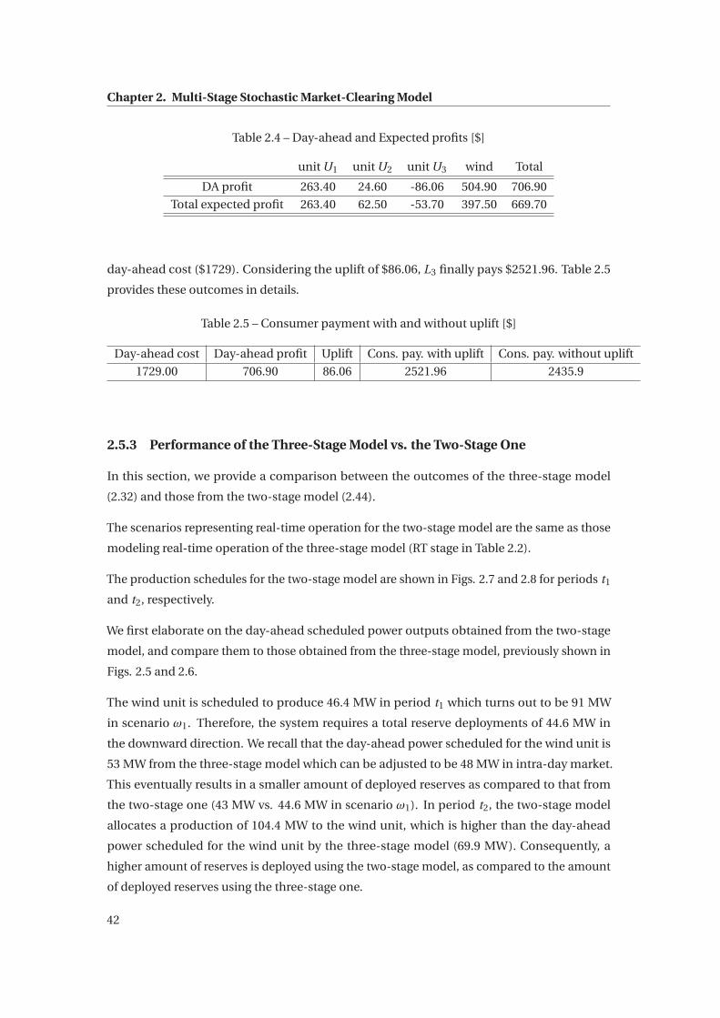
Chapter 2. Multi-Stage Stochastic Market-Clearing Model
Table 2.4 – Day-ahead and Expected profits [$]
unit U1 unit U2 unit U3 wind Total
DA profit 263.40 24.60 -86.06 504.90 706.90
Total expected profit 263.40 62.50 -53.70 397.50 669.70
day-ahead cost ($1729). Considering the uplift of $86.06, L3 finally pays $2521.96. Table 2.5
provides these outcomes in details.
Table 2.5 – Consumer payment with and without uplift [$]
Day-ahead cost Day-ahead profit Uplift Cons. pay. with uplift Cons. pay. without uplift
1729.00 706.90 86.06 2521.96 2435.9
2.5.3 Performance of the Three-Stage Model vs. the Two-Stage One
In this section, we provide a comparison between the outcomes of the three-stage model
(2.32) and those from the two-stage model (2.44).
The scenarios representing real-time operation for the two-stage model are the same as those
modeling real-time operation of the three-stage model (RT stage in Table 2.2).
The production schedules for the two-stage model are shown in Figs. 2.7 and 2.8 for periods t1
and t2, respectively.
We first elaborate on the day-ahead scheduled power outputs obtained from the two-stage
model, and compare them to those obtained from the three-stage model, previously shown in
Figs. 2.5 and 2.6.
The wind unit is scheduled to produce 46.4 MW in period t1 which turns out to be 91 MW
in scenario ω1. Therefore, the system requires a total reserve deployments of 44.6 MW in
the downward direction. We recall that the day-ahead power scheduled for the wind unit is
53 MW from the three-stage model which can be adjusted to be 48 MW in intra-day market.
This eventually results in a smaller amount of deployed reserves as compared to that from
the two-stage one (43 MW vs. 44.6 MW in scenario ω1). In period t2, the two-stage model
allocates a production of 104.4 MW to the wind unit, which is higher than the day-ahead
power scheduled for the wind unit by the three-stage model (69.9 MW). Consequently, a
higher amount of reserves is deployed using the two-stage model, as compared to the amount
of deployed reserves using the three-stage one.
42

2.5. Illustrative Example
Table 2.6 provides the day-ahead and balancing prices obtained from the two-stage model.
The day-ahead prices at period t2 obtained from the two-stage model are higher than those of
the three-stage model. Depending on scenarios, the balancing prices of the two-stage model
are equal to or higher than those obtained from the three-stage model. This is the result of the
reduced wind scenario information in the two-stage model.
Table 2.6 – Clearing prices obtained from two-stage model [$/MWh]
λn λnω1 λnω2 λnω3 λnω4 λnω5 λnω6
period t1 4.01 4.01 4.01 4.01 4.01 4.01 4.01
period t2 5.09 5.09 5.09 5.09 5.09 5.09 5.09
Day-ahead Market
Operation Stage
𝑃 = 102𝑃 = 10𝑃 = 71.6𝑊 = 46.4𝑟 = 17 , 𝑟 = −61.6𝑟 = −24.6𝑟 = −2.6𝑟 = −20.6𝑟 = 4.4𝑟 = 21.4
Figure 2.7 – Scheduled productions and deployed reserves result from two-stage model inperiod t1.
The day-ahead cost expressed in equation (2.1), the expected intra-day cost stated in equation
(2.2), and the expected balancing cost formulated in equation (2.3) are provided in Table 2.7
for both models. The three-stage model results in a higher day-ahead cost than that of the
two-stage model, but a lower balancing cost, which finally results in a lower total expected cost.
The main reason to have a lower day-ahead cost in the two-stage model is scheduled wind
power. The total wind power scheduled is 150.8 MW over the two periods in the two-stage
model, which is higher than 122.6 MW scheduled wind production in the three-stage model.
This, however, results in a higher amount of deployed reserves. That is why the balancing cost
is higher in the two-stage model than that of the three-stage model.
Table 2.8 provides the profit of the units (conventional units and wind unit) at each stage and
in total for both models without uplifts. The total expected profit of producers is lower in
the three-stage model than that in the two-stage model. This observation does not reverse
43

Chapter 2. Multi-Stage Stochastic Market-Clearing Model
Day-ahead Market
Operation Stage
𝑃 = 102𝑃 = 13.6𝑃 = 100𝑊 = 104.4𝑟 = 5.4 , 𝑟 = −82𝑟 = 87.4, 𝑟 = −68𝑟 = 87.4, 𝑟 = −4𝑟 = 13.4𝑟 = 50.4𝑟 = 83.4
Figure 2.8 – Scheduled productions and deployed reserves result from two-stage model inperiod t2.
Table 2.7 – costs [$]; three-stage model vs. two-stage model
Three-stage model Two-stage model
Day-ahead market 1729.00 1540.80
Intra-day market -102.80 –
Real-time Operation -111.10 162.70
Total expected cost 1515.10 1703.50
after adding the uplift, that is $60.86 for the two-stage model and $80.06 for the three-stage
model. Note that the unit profits in real-time operation are zero under the two-stage model;
the reason is that unit U2 and unit U3 are deployed under balancing prices equal to their
marginal costs.
Table 2.8 – Producers profit[$]; three-stage model vs. two-stage model and no uplift
Three-stage model unit U1 unit U2 unit U3 wind all units
Day-ahead 263.40 24.60 -86.00 504.90 706.90
Intra-day -15.30 17.60 9.00 -107.50 -96.20
Real-time operation 15.30 20.30 23.40 0.00 59.00
Total exp. profit 263.40 62.50 -53.70 397.50 669.70
Two-stage model unit U1 unit U2 unit U3 wind all units
Day-ahead 300.07 98.88 -60.86 672.20 1010.30
Real-time operation 0.00 0.00 0.00 0.00 0.00
Total exp. profit 300.07 98.88 -60.86 672.20 1010.30
The consumer payment is the summation of day-ahead cost and day-ahead profit. Given the
44

2.6. Case Studies
day-ahead costs and day-ahead unit profits, the consumer payment without uplift is $2551.1
for the two-stage model and $2435.9 for the three-stage model. That is, the consumer payment
from the two-stage model is higher than that from the three-stage model. Uplift does not
change this result, as it increases the consumer payment to $2611.9 ($2551.1+ uplift of $60.86)
and $2521.9 ($2435.9+ uplift of $80.06) for the two-stage model and the three stage model,
respectively.
2.6 Case Studies
We first present the outcomes of a base case study involving a single load profile. Next, in order
to gain insight on the performance of the three-stage model, we consider different bounds for
the system constraints using the same load profile and explore how these bounds influence
the results. Finally, different load profiles and different bounds are considered.
These case studies aim to appraise the performance of three-stage model by comparing its
outcomes to those from a two-stage model.
2.6.1 Data
We use a 24-node system based on the single-area IEEE Reliability Test System (RTS).
To facilitate the analysis of the results, we have modified some of the original characteristics of
this test system. We consider that the system has 34 lines, 9 conventional generating units,
and 1 wind power unit. The data of conventional generating units are provided in Table 2.9.
We assume that hydro units 2, 4, and 8 (i.e., U50) offer its energy production at zero price.
Table 2.10 provides the total demand over the 24 periods, while the demand locations and the
corresponding shares are provided in Table 2.11.
Table 2.9 – Characteristics of the Generating Units
Type U90 U50 U155 U76 U197 U400
Unit i 1 2,4,8 3,6 5 7 9
Node 2 7,15,22 10,18 16 21 23
P maxi (MW) 90.00 50.00 155.00 76.00 197.00 400.00
P mini (MW) 25.00 15.00 55.00 15.20 69.00 100.00
kSUi ($) 300.00 100.00 320.00 400.00 300.00 1000.00
Ci ($/MW) 19.67 0.00 10.68 11.89 11.09 5.53
The wind power unit is located at node 7. We assume that the wind unit has an installed
45

Chapter 2. Multi-Stage Stochastic Market-Clearing Model
Table 2.10 – Total demand in [MW] from period t1 to period t24
period t1 t2 t3 t4 t5 t6 t7 t8
demand 828.10 831.00 842.00 923.00 943.00 1103.60 1185.30 1139.00
period t9 t10 t11 t12 t13 t14 t15 t16
demand 1137.50 1121.00 1123.00 1099.00 1088.00 1100.00 1103.00 1119.00
period t17 t18 t19 t20 t21 t22 t23 t24
demand 1125.00 1143.00 1115.00 1109.00 1101.20 1080.10 1037.00 800.00
Table 2.11 – Demand location and share
demand L1 L2 L3 L4 L5 L6 L7 L8
location 1 2 3 4 5 6 7 8
share [%] 21.5 16.4 11.7 3.5 5.1 4.8 4.3 4.8
demand L9 L10 L11 L12 L13 L14 L15 L16 L17
location 9 10 13 14 15 16 18 19 20
share [%] 4.1 2 2.4 2.8 2.5 2.6 4.3 3.4 3.8
capacity is 600 MW. To generate wind power scenarios, we use wind speed historical data
from Austin, Texas, which are available in the System Advisor Model (SAM) [2]. To obtain
hourly wind power scenarios for 24 time periods, we apply the power curve of a 2-MW Vestas
V80/2000 wind turbine with a hub height of 80 m. The power curve of this turbine model can
be found in [16].
We should note that we built up the scenarios employing historical data without applying
scenario generation/reduction techniques.
2.6.2 Scenarios
The following process is used for scenario generation. We generate NΩ1 scenarios prior to the
day-ahead gate closure, using all the historical data available up to this time. Each scenario
involves 24 values for the output of the wind power unit pertaining to the 24 time periods of
day d. Then, conditioned to the actual values of each scenario during the hours between the
day-ahead gate closure and the intra-day gate closure, we generate NΩ2 new scenarios for each
one of the original NΩ1 scenarios, resulting in a total number of NΩ scenarios, where NΩ =NΩ1 ×NΩ2 . The decision-making tree is shown in Figure 2.9. For the case study, we consider
10 scenarios at the intra-day market, and corresponding to each second-stage scenario 15
scenarios in real-time operation; therefore, there are in total 150 equi-probable scenarios at
each time period for the three-stage model. The corresponding two-stage model is assumed
46

2.6. Case Studies
Stage 1:Day-ahead
Market
Stage 2:Intra-day
Market
Stage 3:Real-time Operation
Adjustment decisions for
periods 𝑡 ,…, 𝑡 Deployed reserve decisions for periods 𝑡 ,…, 𝑡 in scenario 𝜔Scheduling
decisions for periods 𝑡 ,…, 𝑡
Deployed reserve decisions for periods 𝑡 ,…, 𝑡 in scenario 𝜔Deployed reserve decisions for
periods 𝑡 ,…, 𝑡 in scenario 𝜔
Deployed reserve decisions for periods 𝑡 ,…, 𝑡 in scenario 𝜔
Deployed reserve decisions for periods 𝑡 ,…, 𝑡 in scenario 𝜔
Deployed reserve decisions for periods 𝑡 ,…, 𝑡 in scenario 𝜔
Adjustment decisions for
periods 𝑡 ,…, 𝑡
Figure 2.9 – Scenario tree for the three stages of day-ahead market, intra-day market, andreal-time operation. Each scenario involves 24 values for the wind power output of wind unit.
to have the same 150 equi-probable scenarios in real-time operation.
2.6.3 Base Case
The base case maintains the assumptions used in the example in Section 2.5, namely αWUs1 =αWUs2 = 1.2, αWDs1 =αWDs2 = .8, αΔW = 0.25%, αΔP = 0.25%, and the limit of reserve capacity
is equal to the production capacity of each conventional unit.
Table 2.12 provides details regarding day-ahead profit, expected profit, day-ahead cost, ex-
pected cost, and consumer payment resulting from both models.
Under both models, U90 and U76 incur losses at the day-ahead market, but only U90 has a
negative expected profit. The total day-ahead producer profit is higher in the three-stage
model than in the two-stage model, whereas the total expected profit from the three-stage
model is lower than that of the two-stage model. The main reason is that scheduled power of
the wind unit has a higher value in the three-stage model than in the two-stage one (1471.3
MW vs 1265.5 MW) that translates to a high profit (as its cost is small). This is the result of
47

Chapter 2. Multi-Stage Stochastic Market-Clearing Model
Table 2.12 – Base Case
3-stage Model 2-stage Model
Unit DA Exp. DA Exp.i Profit ($) Profit ($) Profit ($) Profit ($)
1 -8489.42 -4581.29 -10998.97 -3696.75
2 13471.36 13818.44 4575.19 14043.00
3 2175.66 3174.24 3622.79 3896.70
4 13042.15 13400.31 6332.85 14043.00
5 -612.19 282.04 -34.44 136.41
6 2109.44 3269.33 3664.89 3896.70
7 2064.74 2173.20 3435.12 3540.08
8 12954.63 13531.14 4142.90 14043.00
9 42299.73 51345.17 55651.98 59056.00
Wind 16627.21 21358.15 11626.71 11626.71
Total 95643.31 117770.74 82019.03 120584.85
DA Cost ($) Exp. Cost ($) DA Cost ($) Exp. Cost ($)192507.85 174401.51 217498.08 190554.00
Cons. pay. ($) Uplift ($) Cons. pay. ($) Uplift ($)288151.16 9101.61 299517.11 11033.41
information asymmetry on wind production. Also, the day-ahead losses of units U90 and U76
are higher under the two-stage model that make the total day-ahead profit smaller than that
of the three-stage model.
The three-stage model also results in lower day-ahead cost, expected cost, and consumer
payment than those from the two-stage model. The savings in expected cost and consumer
payment obtained in the three-stage model as a percentage of the corresponding values in the
two-stage model are 8.48% and 3.79%, respectively.
For the purpose of comparing day-ahead prices, Fig. 2.10 shows the day-ahead prices obtained
from the three-stage and two-stage models. At period t7 (morning peak), the two-stage model
results in a higher price than that of the three-stage model. Also, at period t24 (when the
lowest load occurs) the price from the three-stage model is considerably lower than that of the
two-stage model.
Despite the higher prices obtained from the two-stage model over several periods, an uplift of
$11,033.41 is still required, and this uplift is higher than the uplift of the three-stage model
($9101.00). As mentioned above, units U90 and U76 incur losses in the day-ahead market under
both models, and thus, they are paid an uplift. Unit U90 is paid an uplift of $8489.42 under
the three-stage model, and $10998.97 under the two-stage model, while Unit U76 receives an
48

2.6. Case Studies
uplift of $612.19 under the three-stage model, and $34.44 under the two-stage model.
2 4 6 8 10 12 14 16 18 20 22 248
10
12
14
16
18
20
period
Day−a
head
Pric
es [$
/MW
h]
price from two−stage model price from three−stage model
Figure 2.10 – Day-ahead clearing prices from the three-stage model and the two-stage modelover all periods.
2.6.4 Analyses of Flexibility of Units for Reserve Provision and Different Adjust-
ment Bounds
The objective of this section is to gain insight on the performance of the three-stage model.
For this purpose, we investigate the impact of the availability of reserves and of diverse limits
on the intra-day power adjustments considering the following cases:
• Case 1 (not limited):
– All conventional units provide reserves: RU,maxi = RD,max
i = P maxi ,∀i .
– Wind production at the day-ahead market is limited by the wind installed capacity.
That is, the limit of the wind unit is 0 ≤Wqt ≤W maxq in the day-ahead market (con-
straint (2.7)). Also, for consistency, 0 ≤Wqt +ΔW Uqtω−ΔW D
qtω ≤W maxq (constraint
(2.17)).
– The up/down wind adjustments are limited by the wind installed capacity at the
intra-day market. That is, ΔW Uqtω ≤ W max
q and ΔW Dqtω ≤ W max
q (i.e., αΔW = 1 in
constraint (2.18)).
– Up/down adjustments of conventional units are up to their maximum power
output. That is, αΔP = 1 in constraint (2.15), and thus, ΔP Ui tω ≤ P max
i and ΔP Di tω ≤
P maxi .
• Case 2 (partly limited):
49

Chapter 2. Multi-Stage Stochastic Market-Clearing Model
Table 2.13 – Savings in the expected cost and consumer payment for the different cases
Saving in Saving inexpected cost (%) consumer payment (%)
Case 1 81.54 63.91
Case 2 8.48 3.79
Case 3 8.19 5.61
– All conventional units provide reserves: RU,maxi = RD,max
i = P maxi ,∀i .
– Wind production at the day-ahead market is limited at ±20% of the best avail-
able wind production forecast. That is, αWDs1 = 0.8 and αWUs1 = 1.2, and thus,
0.8W DAqt ≤Wqt ≤ 1.2W DA
qt (constraint (2.7)).
– The up/down power adjustments of units at the intra-day stage are limited by 25%
of installed capacity. That is, αΔP =αΔW = 0.25, and thus, ΔP Ui tω ≤ 0.25P max
i and
ΔP Di tω ≤ 0.25P max
i , and ΔW Uqtω ≤ 0.25W max
q and ΔW Dqtω ≤ 0.25W max
q .
• Case 3 (highly limited):
– Nuclear and hydro units (U400 and U50) do not provide reserves.
– Wind production at the day-ahead market is limited at ±20% of the best avail-
able wind production forecast. That is, αWDs1 = 0.8 and αWUs1 = 1.2, and thus,
0.8W DAqt ≤Wqt ≤ 1.2W DA
qt (constraint (2.7)).
– The up/down power adjustments of units at the intra-day stage are limited by 25%
of installed capacity. That is, αΔP =αΔW = 0.25, and thus, ΔP Ui tω ≤ 0.25P max
i and
ΔP Di tω ≤ 0.25P max
i , and ΔW Uqtω ≤ 0.25W max
q and ΔW Dqtω ≤ 0.25W max
q .
Fig. 2.11 shows that the total expected profit, the expected cost, and the consumer payment
obtained from the two-stage model are higher than those of the three-stage model. The savings
in expected cost and consumer payment obtained in the three-stage model as a percentage of
the corresponding values in the two-stage model are provided in Table 2.13. The difference
between these outcomes is larger for case 1 (less restricted), and smaller for the more restricted
cases 2 and 3. Therefore, irrespective of the limits imposed on reserves and intra-day unit
adjustments, we conclude that the three-stage model has a better performance from the
consumer point of view.
The uplift, however, follows a different trend (bottom plot in Fig. 2.11). The three-stage model
results in a larger uplift for case 1, while a smaller uplift for case 2 and case 3 than those of the
two-stage model. The uplift from the two-stage model is similar in all cases; however the uplift
50

2.6. Case Studies
from the three-stage model decreases along with the increase in the restrictions. Note that the
uplift amount is small and does not reverse the fact that the consumer payment obtained from
the three-stage model is smaller. Understanding this is easy by observing the day-ahead prices
in Fig. 2.12. The prices from the three-stage model are lower in case 1 than those in cases 2
and 3. This results in smaller uplifts in cases 2 and 3. Also, these prices are of the same order
of magnitude as the day-ahead prices from the two-stage model, and hence, the consumer
payments are of the same order of magnitude in case 2 and case 3. In addition, the day-ahead
prices from the three-stage model and those from the two-stage model get closer to each other
as cases become increasingly restricted.
Case 1 Case 2 Case 30
100200
Expected Profit
K$
Case 1 Case 2 Case 30
100200
Expected Cost
K$
Case 1 Case 2 Case 30
200400
Consumer Payment
K$
Case 1 Case 2 Case 30
1020
Uplift
K$
3−stage model 2−stage model
Figure 2.11 – Expected profit, expected cost, consumer payment, and uplift for different cases.
0 5 10 15 200
10
20
$/M
Wh
Day−ahead Prices
0 5 10 15 200
10
20
$/M
Wh
0 5 10 15 200
10
20
Time period
$/M
Wh
3−stage model 2−stage model
Case 1
Case 2
Case 3
Figure 2.12 – Day-ahead clearing prices for different cases
We also simulate these models on different load profiles (shown in Fig. 2.13) and observe
similar outcomes.
51

Chapter 2. Multi-Stage Stochastic Market-Clearing Model
Fig. 2.14 shows that a higher expected cost is obtained by using the two-stage model than that
of the three-stage model irrespective of the limiting bounds for five different load profiles and
the different cases. Note that the large difference between expected costs of the three stage
model and the two stage model for case 1 is due to the wide (and rather unrealistic) bounds
assumed for the intra-day power adjustments of the wind unit as well as conventional units.
The expected costs of the three-stage model get closer to those from the two-stage model
when bounds become tighter, as in case 2 and case 3.
0 5 10 15 20600
700
800
900
1000
1100
1200Different load profiles (inflexible load)
Periods
MW
profile1profile2profile3profile4profile5
Figure 2.13 – Different load profiles
Case 1 Case 2 Case 30
20
40
60
80
100
120
140
160
180Expected Cost
K$
load profile1load profile2load profile3
load profile5load profile4
3−stage 2−stage 3−stage 2−stage 3−stage 2−stage
Figure 2.14 – Expected costs for different load profiles and different limited cases
Table 2.14 provides the savings in expected cost and consumer payment obtained in the
three-stage model as a percentage of the corresponding values in the second-stage model.
The savings in case 1 are large due to the wide bounds assumed for the intra-day power
adjustments of the wind unit as well as the conventional units.
52

2.6. Case Studies
Table 2.14 – Savings in expected cost and consumer payment for the different load profiles [%]
Savings in Exp. Cost Savings in Consumer Pay.
Load profile case 1 case 2 case 3 case 1 case 2 case 3
1 86.80 9.72 9.07 75.78 6.29 11.85
2 86.85 9.75 9.16 74.60 6.34 11.94
3 87.07 9.79 9.20 73.75 6.71 12.63
4 83.36 7.66 7.28 66.22 3.18 5.42
5 83.42 8.71 7.93 67.44 7.57 8.75
In addition to the expected value, another metric to evaluate the performance of stochastic
optimization problems is the standard deviation. It is desirable to have a cost with both small
expected value and small variance, since this means that the operation cost is expected to be
small with a low probability of obtaining a cost very different from the expected cost.
The standard deviations for the different load profiles considered and the different cases
analyzed are provided in Table 2.15.
The standard deviations of both models are of the same order of magnitude for case 1 (all
load profiles). For case 2, the standard deviations from the two-stage model are smaller than
those from the three-stage model. This observation is, however, reversed for case 3. Therefore,
a general conclusion regarding the standard deviation of cost from these instances cannot
be obtained. In other words, none of these models guarantee a smaller variability of cost
as compared to the other one. That is, the three-stage model improves the cost in term of
expectation, but the variability of the cost around the expected value is similar to that of the
two-stage model.
Table 2.15 – Standard deviations from the three-stage model and the two-stage model for thedifferent load profiles [$]
Case 1 Case 2 Case 3
Load 3-stage 2-stage 3-stage 2-stage 3-stage 2-stage
profile model model model model model model
1 1.10×10⁴ 3.61×10⁴ 3.08×10⁴ 7.45×10³ 7.58×10³ 1.32×10⁴
2 1.05×10⁴ 3.53×10⁴ 3.04×10⁴ 6.71×10³ 9.20×10³ 1.18×10⁴
3 9.30×10³ 4.33×10⁴ 2.95×10⁴ 7.84×10³ 6.28×10³ 1.21×10⁴
4 1.09×10⁴ 4.52×10⁴ 3.57×10⁴ 6.76×10³ 1.02×10⁴ 1.34×10⁴
5 1.19×10⁴ 4.04×10⁴ 3.28×10⁴ 1.44×10⁴ 7.34×10³ 8.74×10³
Finally, the VSS calculated for the three-stage model is compared with that of the two-stage
53

Chapter 2. Multi-Stage Stochastic Market-Clearing Model
model. The results are provided in Table 2.16.
The three-stage model has a better performance than the two-stage model (i.e, higher VSS) for
all case studies except for those pertaining to load profile 4. In this case, the use of the optimal
first-stage solution of the deterministic model without recourse, denoted by xMV in Section
2.4.3, causes load-shedding in real-time operation, where the wind power output is realized
under the two-stage model. This results in a high cost, and consequently, a large difference
between the optimal value of the two-stage model and that of the deterministic model.
Table 2.16 – The VSS [%]
Three-stage model Two-stage model
Load profile case 1 case 2 case 3 case 1 case 2 case 3
1 4.94 0.32 0.31 0.01 0.01 0.01
2 4.96 0.12 0.11 0.01 0.01 0.01
3 5.06 0.23 0.22 0.01 0.01 0.01
4 3.79 1.31 1.30 6.19 6.19 6.19
5 3.71 0.22 0.22 1.41 1.41 1.41
2.6.5 Computation Time
In this section, we elaborate on the computational aspect of the proposed model by consider-
ing different number of scenarios and different number of units.
For the simulations, we use CPLEX 12.5.0 under MATLAB on a computer with two Intel(R)
Core(TM) processors clocking at 2.7 GHz and 8 GB of RAM. The sizes of the proposed models
in terms of numbers of variables and constraints, and computation time for the base case are
provided in Table 2.17.
Table 2.17 – Dimension of the three-stage and two-stage models (base case)
3-stage Model 2-stage Model
No. of binary variables 216 216
No. of continuous variables 375432 217232
No. of total variables 375648 217248
No. of constraints 786744 409320
Computation time (s) 123 48
We should note that the computation times reported are an indication of the tractability of a
three-stage model, and that using industry-grade computers and parallelization should allow
54

2.6. Case Studies
achieving the required solution times.
First, we fix the number of scenarios to 15 in the third stage and consider different numbers of
scenarios in the second stage. The corresponding computation time and the expected cost are
provided in Table 2.18.
The computation time increases with the problem size. However, it remains within an accept-
able range (e.g., less than 8 minute for a problem size larger than 0.7 million variables and 1.5
million constraints). The increases in the total number of scenarios (from 150 to 225 and from
150 to 300) result in the same expected cost, which is slightly higher than the expected cost
obtained in the case with 150 scenarios. In other words, the sensitivity of the expected cost
decreases as the number of second-stage scenarios increases.
Table 2.18 – Computation time for different number of scenarios in the second stage (10 units,24 buses, 15 scenarios in the third stage)
No. of scenarios in the second stage 10 15 20
No. of scenarios in the third stage 15 15 15
Total No. of scenarios 150 225 300
Total No. of constraints 786,744 1,179,264 1,571,784
Total No. of decision variables 375,648 562,848 750,048
Expected cost ($) 1.74×10⁵ 1.77×10⁵ 1.77×10⁵
Computation time (s) 123 235 445
Table 2.19 provides the computation time for different number of the scenarios in the third
stage if the number of the second-stage scenarios is fixed to 10. The computation time does
not change significantly from 150 scenarios to 250 scenarios, while it increases to 491 s if
considering 350 scenarios, for which the size of the problem is significantly larger (i.e., 0.9
million variables and 1.8 million constraints). The increases in the total number of scenarios
(from 150 to 250 and from 150 to 350) result in the same expected cost, which is slightly higher
than the expected cost obtained in the case with 150 scenarios. In other words, the sensitivity
of the expected cost decreases as the number of third-stage scenarios increases.
Given Tables 2.19 and 2.18, we infer that the sensitivity of the expected cost decreases as the
total number of scenarios increases.
In short, an increase in the number of scenarios involves a better uncertainty description, and
hence, a possible change in expected cost. However, this is valid up to a certain number of
scenarios (in the case study, 225). Once this number of scenarios is reached, the uncertainty
description is accurate enough and the expected cost remains unaltered. If this number of
55

Chapter 2. Multi-Stage Stochastic Market-Clearing Model
Table 2.19 – Computation time for different number of scenarios in the third stage (10 units,24 buses, 10 scenarios in the second stage)
No. of scenarios in the second stage 10 10 10
No. of scenarios in the third stage 15 25 35
Total No. of scenarios 150 250 350
Total No. of constraints 786,744 1,317,144 1,847,544
Total No. of decision variables 375,648 562,848 750,048
Expected cost ($) 1.74×10⁵ 1.77×10⁵ 1.77×10⁵
Computation time (s) 123 147 491
scenarios is increased, the expected cost remains the same, whereas the computation time
increases.
Table 2.20 – Computation time for the different number of generators (24 buses, 150 scenarios)
No. of units 10 15 20
No. of binary variables 216 336 456
Total No. of decision variables 375,648 448,008 520,368
Total No. of constraints 786,744 964,944 1,143,144
Expected cost ($) 1.74×10⁵ 1.75×10⁵ 1.75×10⁵
Computation time (s) 123 182 590
Finally, Table 2.20 provides computation times for different number of units if 150 scenarios
are considered. With the increase in the number of units, the size of the problem and the
number of binary commitment variables increase, and hence, the computation time increases
as well.
2.6.6 Case Study Conclusion
We present a three-stage stochastic model to clear the day-ahead market, which explicitly
represents an intra-day market and real-time operation. We then compare the outcomes of
this model with results from a two-stage model, which includes a prognosis solely of real-time
operation.
The simulation outcomes show that the proposed three-stage model has a better performance
than the two-stage one as a result of more informed decisions at the day-ahead market. That
is, the three-stage model results in lower day-ahead cost, expected cost, total expected profit,
and consumer payment than those from the two-stage model.
56

2.7. Summary and Conclusion of the Chapter
Additionally, the day-ahead peak prices obtained from the three-stage model are lower than
those from a two-stage model. This results from the use of information about evolving wind
power forecast across market stages in the three-stage model, and therefore, more efficient
“positioning” of the units in term of day-ahead power production schedules, as well as intra-day
power adjustments and deployed reserves.
The VSS also confirms that the use of three-stage model is beneficial to a system with a large
amount of uncertain wind production over a two-stage one.
Regarding computation time, our analyses show that although the computation time increases
with the problem size, it remains still within an acceptable range. The sensitivity of the
expected cost decreases as the number of the scenarios increases. An increase in the number
of scenarios involves a better uncertainty description (and consequently a possible change in
the expected cost), but up to a certain number of scenarios. Once this number is reached, the
uncertainty description cannot improve additionally and the expected cost remains the same,
whereas the computation time increases. The computation times reported are an indication
of the tractability of a three-stage model. Using industry-grade computers and parallelization
techniques should help achieving the required solution times.
The remarks above are concluded by applying the three-stage model to different load profiles,
and by considering different limits on adjustment bounds and flexibility of units to provide
reserves. Our simulation results indicate that the outcomes from the three-stage model and
the two-stage one get closer as restrictions get tighter. The small bounds are translated into
less energy trading in the intra-day market, and hence, the results of the three-stage model get
closer to those from two-stage one.
These outcomes suggest that replacing a deterministic model with a three-stage model, not a
two-stage one, has clear advantages. In other words, if the industry decides to move toward
using a a stochastic clearing algorithm (and if it has sufficient computational resources to do
so), such a clearing algorithm should be a three-stage one, not a two-stage one.
2.7 Summary and Conclusion of the Chapter
The evolving market conditions, including an increasing number of intra-day markets (from
the energy trading point of view) and the growth of renewable generation (from the technology
point of view), call for a revise in market-clearing models.
With the aim of obtaining better informed day-ahead decisions, we propose a multi-stage
stochastic clearing model. In other words, we argue that if the use of a stochastic clearing
57

Chapter 2. Multi-Stage Stochastic Market-Clearing Model
model is adopted in systems with a large amount of renewable production, it should be a
multi-stage stochastic model, and not a two-stage one.
In a multi-stage clearing model, not only different realizations of renewable power output are
considered, but also how these realizations evolve from day-ahead forecasts into real-time
values are taken into account. A multi-stage model allocates flexibility for the contribution
of renewable production in both the day-ahead and intra-day markets in form of scheduled
productions and their adjustments. In other words, the information on how uncertain re-
newable production develops across the market floors, as well as, allowing flexibility for the
contribution of renewable generation in both the day-ahead and intra-day markets improve
the market outcomes and integration of renewable generation.
58

3 Pricing Schemes Pertaining to A
Stochastic Non-Convex Market-
Clearing Model3.1 Introduction
When it comes to electricity markets, an accurate modeling of the underlying physics of power
systems is important to obtain right market outcomes. Market outcomes include scheduled
power productions that must respect the non-continuous operating nature (non-convexities)
of power system elements, in particular generating units.
To precisely model non-convexities pertaining to the technical characteristics and operation
conditions of power system elements, integer variables are the key. For instance, to model
physical conditions of generating units such as the start-up and shut-down sequences, binary
variables are used. Therefore, the corresponding clearing problem is formulated as a Mixed-
Integer Linear Programming problem (MILP). Although the MILP problem allows to obtain
production schedules consistent with the operation conditions of the power system, it results
in a number of challenges pertinent to economic aspects of the market.
To trade the electric energy, marginal prices are recognized to provide the right market signals
in competitive markets, as they are appropriate prices to achieve short-term economic effi-
ciency and long-term cost recovery [53]. Among other relevant properties of marginal prices,
reaching market equilibrium is a distinguished feature. In an equilibrium, market prices are
such that all participants are better off to follow market outcomes. That is, no agent incurs
losses under these prices and no agent earns a higher profit by deviating from the schedule
assigned. This implies that market players have no incentive to submit inaccurate information.
In other words, marginal pricing promotes truth-telling in the market [61]. Marginal prices
can be obtained as dual variables of power balance equations for convex market-clearing
problems. This connection is, however, missing in MILP problems due to the inherent non-
convex structure, which often leads to a non-zero duality gap between the primal and dual
59

Chapter 3. Pricing Schemes Pertaining to A Stochastic Non-Convex Market-ClearingModel
counterparts.
In the presence of non-convexities, different pricing approaches are proposed to tackle this
problem in practice. As a solution, [46] proposes to fix the integer decisions at their optimal
values obtained from sloving the MILP model, and to derive prices from the dual problem of
the resulting continuous primal problem. The clearing prices obtained from this approach are
the closest valid prices that can be defined for the corresponding non-convex clearing problem.
This approach seems to be satisfactory in practice, as PJM follows a similar implementation
[46] . However, obtaining prices from the dual problem of a relaxed continuous version of the
original MILP clearing problem may yield situations where some producers cannot recover
their costs. The reason is that such pricing approaches do not fully reflect costs pertaining to
discrete decisions, such as the start-up cost of a unit. In other words, the prices obtained do not
encompass cost-recovery of discontinuous costs. Such marginal prices may lead to situations
where financial losses occur to an extent that the corresponding producers may leave the
market. This may eventually lead to a financial loss of welfare and market inefficiency.
To mitigate this problem, a common practice is to compensate each producer incurring losses
through a side-payment called uplift. A simple example is as follows. Suppose that a thermal
unit is scheduled to generate a certain power under a marginal price which is equal to its
marginal production cost. Therefore, the unit cannot recover its start-up cost. This fixed cost
is, thus, compensated using an uplift, which is paid by all demands to this thermal unit. In
such a situation, the owner of the unit may try to suggest a higher start-up cost than its real
one to earn more money by being paid a higher uplift than the actual cost.
This example shows that uplift is not economically a neat concept. Uplifts do not promote
truth-telling in the market, rather they encourage strategic pay-as-bid behavior. The uplifts are
discriminatory, and their implementation requires a detailed regulation. Hence, alternative
pricing methods in non-convex electricity markets are of interest of the electricity market
community.
Thus far, we have described the existing pricing issue in deterministic markets. As presented in
the previous chapter, a high penetration of renewable generation calls for the use of stochastic
market-clearing models, where the system power balance results in a significant connec-
tion between power production schedules in the day-ahead market, power adjustments in
intra-day markets, and deployed reserves in real-time operation. These connections in the
quantities of different market stages result in links between the prices obtained from the
corresponding market stages. Therefore, moving toward the use of stochastic market-clearing
models increases the degree of complexity of the pricing problem.
60

3.2. A New Pricing Mechanism with Cost Recovery
In short, in a system with a large amount of renewable generation, day-ahead prices are
effected by non-convexities due to operational conditions, as well as by uncertainty associated
with renewable generation. In this context, we strive to derive a new pricing scheme with
the aim of obtaining a set of uniform day-ahead prices with cost-recovery properties at the
crossroads of stochasticity and non-convexity.
3.2 A New Pricing Mechanism with Cost Recovery
We, first, elaborate on the desired properties that a pricing scheme is expected to meet.
Our focus is to obtain a set of day-ahead prices in a market environment with stochastic renew-
able generation. A desired property of these prices is to reflect the uncertainty associated to
renewable generation. Therefore, these prices must be obtained from a model which appropri-
ately considers stochastic renewable generation. Referring to Chapter 2, to optimally integrate
renewable generation, the power production outputs of conventional units (e.g., thermal and
hydro units) are scheduled in the day-ahead market considering all possible realizations of
renewable generation at real-time operation. Therefore, the day-ahead scheduled produc-
tions are affected by stochastic generation, and the day-ahead prices as well. In other words,
uncertain renewable generation transfers its impact on day-ahead prices through day-ahead
scheduled productions. Furthermore, realizations of renewable production require reserve
deployments in real-time operation, and consequently, result in balancing prices which are
linked to the day-ahead prices. That is, uncertain renewable generation has additionally an
impact on day-ahead prices through balancing prices.
Therefore, explicitly modeling the sequence of decision-making process is important. This
entails the day-ahead market, a number of intra-day markets, and real-time operation, and
implies the use of a multi-stage stochastic clearing model, similar to the one proposed in
Chapter 2.
The marginal prices obtained using the conventional pricing approach do not embody cost-
recovery features. This motivates a new pricing mechanism, where day-ahead prices guarantee
cost-recovery conditions to producers. The cost-recovery conditions need to be defined in
the presence of high renewable production, and then, considered as market constraints in a
clearing model. Such a clearing model results in marginal prices with cost-recovery features
that eliminate a need for uplifts.
We should note here that two types of uplift are identified by economists: make-whole pay-
ments and lost opportunity profits.
61

Chapter 3. Pricing Schemes Pertaining to A Stochastic Non-Convex Market-ClearingModel
Make-whole payments ensure that each unit can recover its incurred cost by producing the
energy at the level assigned to it in the market. This type of uplift does, therefore, focus on the
production cost of the unit (marginal production cost and fixed cost). On the other hand, the
uplift related to lost opportunity profits ensures that each online unit receives its maximum
possible profit under the existing market prices. Some units may be willing to produce more
under the final prices, but fulfilling such a wish may not be possible as it may cause that the
market would not be in equilibrium. A solution to encourage units to still follow the assigned
productions is to pay them their lost opportunity profits through a side-payment.
Our focus is to remove the need for uplift in term of make-whole payments. Therefore, the
final day-ahead prices provided by the methodology proposed may cause some units to
experience lost opportunity profits. That is, considering the final prices some units are willing
to produce more, but this is not possible for the market to be in equilibrium. Uplifts (of
reduced magnitude) can be used to remedy this side effect and to cover the lost opportunity
revenue. These uplifts are then socialized among consumers. For the sake of simplicity, we do
not consider the lost opportunity profits.
Finally, the new day-ahead prices obtained shall deviate in the least possible manner from
conventional marginal prices. This implies that social welfare deviates the least from its
maximum value.
Regarding the desired properties above and inspired by the approach in [59], we provide a
pricing scheme for a non-convex stochastic clearing model such that the producers do not
incur losses.
The proposed approach is as follows:
1. We formulate a stochastic market-clearing model with binary unit-commitment vari-
ables, which results in a MILP problem.
2. The binary variables are relaxed to be continuous to obtain a relaxed linear primal
problem.
3. The dual of the relaxed linear primal problem is then obtained.
4. Next, we formulate a primal-dual minimization problem whose objective function is
the duality gap and that is subject to primal and dual constraints. Since the integrity
constraints of the primal problem are also included, the primal-dual problem is a
MILP. The quantities and prices are output of this model. It is important to note that
minimizing the duality gap is tantamount of getting as close as possible to maximum
welfare, but ensuring cost recovery.
62

3.3. Assumptions
5. To guarantee cost recovery for producers, we incorporate cost-recovery equations as
extra constraints in the primal-dual problem.
In the presence of stochasticity, the definition of cost-recovery conditions for producers is not
unique. In this sense, three views can be expressed:
1. Cost-recovery conditions in the day-ahead market: To satisfy cost-recovery conditions
in the day-ahead market, the day-ahead prices must ensure that the day-ahead profit of
each unit is not negative. That is, the day-ahead revenues minus the day-ahead costs
(including marginal production costs and fixed costs) must be either zero or a positive
value.
2. Cost-recovery conditions in expectation: In the same vein, cost-recovery conditions in
expectation are imposed. That is, average cost recovery of each unit over all realizations
of stochastic generation is guaranteed, i.e., the expected revenue minus the expected
cost of each unit is required to be non-negative.
3. Cost-recovery conditions per scenario: The most conservative interpretation of cost-
recovery conditions indicates that for each individual realization of stochastic genera-
tion the per scenario profit of each unit is required to be non-negative.
3.3 Assumptions
We consider the following assumptions to formulate the proposed pricing optimization model.
Many of these assumptions are similar to those stated in Section 2.3.
• The uncertain renewable resource is wind power generation. Wind generation leads
renewable production in term of installed capacity and technological development
[31]. Considering other stochastic resources does not change the nature of the model
proposed.
• The production of wind units depends on the uncertain wind power realization. Wind
power production is represented using scenarios. These scenarios are built using his-
torical wind production data as samples without applying any scenario generation and
scenario reduction techniques.
• The wind producers are assumed to offer their production at zero cost. This is in line
with the actual market practice of wind production in some countries, where as much
wind generation as possible shall be absorbed.
63

Chapter 3. Pricing Schemes Pertaining to A Stochastic Non-Convex Market-ClearingModel
• We assume that loads are deterministic. This assumption allows focusing on wind
uncertainty. Note that in systems with imperfect wind power production, load variability
is generally small in comparison with wind uncertainty.
• Loads are assumed to be inelastic. This assumption can easily be removed from the
model without modeling or computational complications.
• Generation cost functions are assumed to be linear for simplicity. However, note that
quadratic cost functions can be accurately approximated using piecewise linear func-
tions. Also, all generating units are required to offer their energy at marginal costs.
• The costs of the deployed reserves is assumed to be equal to the cost of producing
energy. Other criteria about the cost of the deployed reserves could be straightforwardly
considered in the proposed formulation.
• The stochastic clearing model co-optimizes energy and reserve deployment without ex-
plicit reserve offers in the day-ahead market. Units and flexible demands can specify the
reserve levels that they are willing to provide, and hence, we given them the opportunity
of reserve deployment for a profit.
• A linear representation of the transmission network is considered through a dc load flow
model where losses are neglected.
• We do not consider security criteria, such as n-1, to focus on the analyses of wind
uncertainty, and also, to avoid an increase in the size of the model which consequently
leads to an increase in computation time.
• The non-convexities considered are solely those due to non-zero minimum power
outputs of conventional units, start-up costs, and binary unit-commitment variables.
Taking into account other source of non-convexities, such as shut-down costs and
minimum up/down time constraints, is straightforward.
These assumptions are made for convenience, simplicity, and the sake of computational
tractability.
3.4 Decision-Making Process
The decision-making process is based on the multi-stage stochastic clearing model described
in Section 2.2. To reduce complexity but still satisfying the need for a stochastic clearing model
in the presence of uncertainty, we consider the two-stage model (2.44) in this chapter. Note
64

3.5. Model Description
that the principles of the proposed pricing approach are fully applicable to any multi-stage
stochastic clearing model, and the use of two-stage model is for the sack of simplicity.
The decision-making sequence involves day-ahead market and real-time operation. The day-
ahead outcomes, including scheduled power outputs and prices, are here-and-now decisions
as they are made before uncertain parameters are realized, while in real time deployed reserves
(balancing actions) and balancing prices represent wait-and-see decisions which are recourse
actions taken after uncertainty realizes.
3.5 Model Description
In this section, we provide the mathematical description of the proposed pricing scheme. For
this purpose, we first present the primal two-stage clearing model in Section 3.5.1. Next, We
formulate the corresponding dual problem in Section 3.5.2, and the corresponding primal-dual
problem in Section 3.5.3. Section 3.5.4 provides mathematical descriptions of cost-recovery
conditions for units. Next, the linearization of cost-recovery conditions is presented in Section
3.5.5. Finally, we provide the complete linear mixed-integer model in Section 3.5.6.
3.5.1 Primal Problem: Two-Stage Clearing Model
The first step of the proposed pricing approach is to formulate a two-stage clearing model. We
take the two-stage model (2.44) and skip to elaborate on the details as this model is described
in details in Section 2.4. We just slightly modify the two-stage model (2.44) according to the
simplifying assumptions indicated in Section 3.3. These modifications are related to wind
production as follow.
The wind producers are assumed to offer their production at zero cost. That is, Cq is zero in the
cost function (2.34). Therefore, the objective function includes the following two components:
• The day-ahead cost involving the start-up costs and production costs of conventional
units over all periods of the market horizon:
NT∑t=1
NG∑i=1
(C SUi t +Ci Pi t ) (3.1)
• The expected balancing cost involving the cost of deployed reserves and involuntary
65

Chapter 3. Pricing Schemes Pertaining to A Stochastic Non-Convex Market-ClearingModel
load shedding:
NΩ∑ω=1
πω
[ NT∑t=1
( NG∑i=1
Ci (r Ui tω− r D
i tω)+NL∑j=1
V LOLj t Lshed
j tω
)](3.2)
Additionally, we assume that wind power output can be scheduled within a range of zero and
the installed capacity in the day-ahead market. Therefore, constraint (2.7) changes to:
0 ≤Wqt ≤W maxq (3.3)
The formulation of the two-stage MILP clearing model is provided in the following. We should
note that the corresponding dual variables are listed in front of the constraints that are used
when formulating the dual problem.
MinimizeΞp
NT∑t=1
NG∑i=1
C SUi t +
NΩ∑ω=1
πω
[ NT∑t=1
( NG∑i=1
Ci (Pi t + r Ui tω− r D
i tω)+NL∑j=1
V LOLj t Lshed
j tω
)](3.4a)
subject to
Day-ahead constraints:∑i∈M G
n
Pi t +∑
q∈M Qn
Wqt −∑
j∈M Ln
L j t −∑
r∈Λn
Bnr (θnt −θr t ) = 0 : (λnt ),∀n,∀t (3.4b)
− f maxnr ≤ Bnr (θnt −θr t ) ≤ f max
nr : (ε−maxnr t ,εmax
nr t ),∀n,∀r ∈Λn ,∀t (3.4c)
ui t P mini ≤ Pi t ≤ ui t P max
i : (φmini t ,φmax
i t ),∀i ,∀t (3.4d)
Wqt ≤W maxq : (ρW
qt ),∀q,∀t (3.4e)
K SUi (ui t −ui ,t−1) ≤C SU
i t : (βi t ),∀i ,∀t (3.4f)
RDi ≤ Pi t −Pi ,t−1 ≤ RUi : (ψmini t ,ψmax
i t ),∀i ,∀t (3.4g)
θ1t = 0 : (σ1t ),∀t (3.4h)
ui t ∈ {0,1},∀i ,∀t (3.4i)
Real-time operation constraints:∑i∈M G
n
(r Ui tω− r D
i tω)+ ∑q∈M Q
n
(W RTqtω−Wqt −w spill
qtω )
+ ∑r∈Λn
Bnr (θnt −θntω−θr t +θr tω)+ ∑j∈M L
n
Lshedj tω = 0 : (λntω),∀n,∀t ,∀ω (3.4j)
− f maxnr ≤ Bnr (θntω−θr tω) ≤ f max
nr : (ε−maxnrωt ,εmax
nrωt ),∀n,∀r ∈Λn ,∀t ,∀ω (3.4k)
Pi t + r Ui tω− r D
i tω ≤ ui t P maxi : (φmax
i tω ),∀i ,∀t ,∀ω (3.4l)
66

3.5. Model Description
−Pi t − r Ui tω+ r D
i tω ≤−ui t P mini : (φmin
i tω ),∀i ,∀t ,∀ω (3.4m)
RDi ≤(Pi t + r U
i tω− r Di tω
)− (Pi ,t−1 + r U
i ,t−1,ω− r Di ,t−1,ω
)≤ RUi :
(ψmini tω ,ψmax
i tω ),∀i ,∀t ,∀ω (3.4n)
r Ui tω ≤ RU,max
i t : (αUi tω),∀i ,∀t ,∀ω (3.4o)
r Di tω ≤ RD,max
i t : (αDi tω),∀i ,∀t ,∀ω (3.4p)
Łshedj tω ≤ L j t : (μ j tω),∀ j ,∀t ,∀ω (3.4q)
w spillqtω ≤W RT
qtω : (γqtω),∀q,∀t ,∀ω (3.4r)
θ1tω = 0 : (σ1tω),∀t ,∀ω (3.4s)
Variable declarations:
0 ≤ Pi t ,C SUi t ,∀i ,∀t
0 ≤Wqt ,∀q,∀t
0 ≤ r Ui tω,r D
i tω,∀i ,∀t ,∀ω0 ≤ w spill
qtω ,∀q,∀t ,∀ω0 ≤ Lshed
j tω ,∀ j ,∀t ,∀ω (3.4t)
The problem (3.4) minimizes the expected operation cost (3.4a) considering day-ahead schedul-
ing constraints (3.4b)-(3.4i), real-time operation constraints (3.4j)-(3.4s), and variable declara-
tions (3.4t). The minimization is over the set of primal variablesΞp = {C SUi t ,ui t ,Pi t ,∀i ,∀t ;Wqt ,
∀q,∀t ;θnt ,∀n,∀t ;r Ui tω,r D
i tω,∀i ,∀t ,∀ω; wspillqtω ,∀q,∀t ,∀ω;θntω,∀n,∀t ,∀ω;Lshed
j tω ,∀ j ,∀t ,∀ω; }, as
described in Chapter 2.
3.5.2 Dual Problem of Two-stage Clearing Model
The second step of the proposed approach is to obtain a dual formulation of the primal
clearing model (3.4). For this purpose, the integrity constraint (3.4i) in problem (3.4) is relaxed
to be:
0 ≤ ui t ≤ 1,∀i ,∀t : (υmini t ,υmax
i t ) (3.5)
where υmini t and υmax
i t are the corresponding dual variables.
This relaxed problem is a simple linear program whose dual problem is straightforward to be
obtained.
As a reminder, the dual problem of the LP problem in general from (3.6) is formulated in (3.7)
67

Chapter 3. Pricing Schemes Pertaining to A Stochastic Non-Convex Market-ClearingModel
[36].
Minimizex≥0
cTx (3.6a)
subject to:
Ax ≥ b, (μ) (3.6b)
C x = d, (λ) (3.6c)
where x ∈Rn , c ∈Rn , A ∈Rm×n , b ∈Rm, C ∈Rq×n , and d ∈Rq .
Maximizeμ≥0,λ
bTμ+d Tλ (3.7a)
subject to: ATμ+C Tλ≤ c (3.7b)
where μ ∈Rm and λ ∈Rq .
In the same vein, the dual formulation of relaxed primal problem (3.4) is:
MaximizeΞd∑
t
[− ∑n, j∈M L
n
λnt L j t −∑
n,r∈Λn
( f maxnr εmax
nr t − f maxnr ε−max
nr t )+∑i
(−υmaxi t −ψmax
i t RUi +ψmini t RDi )
+∑ω
(−∑
qγqtωW RT
qtω−∑jμ j tωL j t −
∑iψmax
i tω RUi +∑
iψmin
i tω RDi
−∑iαU
i tωRU,maxi t −∑
iαD
i tωRD,maxi t − ∑
n,r∈Λn
( f maxnr εmax
nr tω− f maxnr ε−max
nr tω ))]
(3.8a)
subject to
Ci +λnt +ρi t +ψmaxi t +ψmin
i t +ψmaxi tω −ψmin
i tω +φmaxi tω −φmin
i tω ≥ 0,∀i ∈ M Gn ,∀n,∀ω,∀t
(3.8b)
λnt +λntω+ρWqt ≥ 0,∀q ∈ M L
n ,∀n,∀ω,∀t (3.8c)
1−βi t ≥ 0,∀i ,∀t (3.8d)
πωCi +λntω+ψmaxi tω −ψmin
i tω +αUi tω+φmax
i tω −φmini tω ≥ 0,∀i ∈ M G
n ,∀n,∀ω,∀t (3.8e)
−πωCi −λntω−ψmaxi tω +ψmin
i tω −αDi tω−φmax
i tω +φmini tω ≥ 0,∀i ∈ M G
n ,∀n,∀ω,∀t (3.8f)
σ1t|n=1+ ∑
r∈Λn
Bnr (εmaxnr t −ε−max
nr t )− ∑r∈Λn
Bnr
(λnt −λr t +λntω−λr tω
)= 0,∀n,∀ω,∀t
(3.8g)
σ1tω|n=1+ ∑
r∈Λn
Bnr (εmaxnr t −ε−max
nr t )+ ∑r∈Λn
Bnr (λntω−λr tω) = 0,∀n,∀ω,∀t (3.8h)
68

3.5. Model Description
βi t K SUi −φmax
i t P maxi +φmin
i t P mini −φmax
i tω P maxi +φmin
i tω P mini +υmax
i t ≥ 0,∀i ,∀ω,∀t (3.8i)
πωV LOLj t +λntω+μ j tω ≥ 0,∀ j ∈ M L
n ,∀n,∀ω,∀t (3.8j)
λntω+γqtω ≥ 0,∀q ∈ M Qn ,∀ω,∀t (3.8k)
εmaxnr t ,ε−max
nr t ≥ 0,∀n,∀r ∈Λn ,∀t (3.8l)
εmaxnr tω,ε−max
nr tω ≥ 0,∀n,∀r ∈Λn ,∀ω,∀t (3.8m)
υmaxi t ,βi t ,φmax
i t ,φmini t ,ψmax
i t ,ψmini t ≥ 0,∀i ,∀t (3.8n)
ρWqt ≥ 0,∀q,∀t (3.8o)
φmaxi tω ,φmin
i tω ,ψmaxi tω ,ψmin
i tω ,αUi tω,αD
i tω ≥ 0,∀i ,∀ω,∀t (3.8p)
μ j tω ≥ 0,∀ j ,∀ω,∀t , γqtω ≥ 0,∀q,∀ω,∀t (3.8q)
where Ξd = {λnt ,∀n,∀t ;λntω,∀n,∀t ,∀ω;εmaxnr t ,ε−max
nr t ,∀n,∀r ∈ Λn ,∀t ;εmaxnr tω,ε−max
nr tω ,∀n,∀r ∈Λn ,∀t ,∀ω;φmax
i t ,φmini t ,υmax
i t ,βi t ,ψmaxi t ,ψmin
i t ,∀i ,∀t ;ρWqt ,∀q,∀t ;φmax
i tω ,φmini tω ,ψmax
i tω ,ψmini tω ,αU
i tω,
αDi tω,∀i ,∀t ,∀ω;μ j tω,∀ j ,∀t ,∀ω;γqtω∀q,∀t ,∀ω} are the variables of the dual problem.
Among them and of utmost importance are λnt and λntωπω
which are the day-ahead prices and
probability-removed balancing prices, respectively.
3.5.3 Primal-Dual Problem
The next step is to formulate the primal-dual form of problem (3.4). The advantage of the
primal-dual problem is to allow simultaneously controlling primal variables, i.e., quantities,
and dual variables, i.e., prices.
To obtain the primal-dual formulation, we proceed as follows. We first provide the primal-dual
formulation in general form using the LP problem (3.6) and its dual problem (3.7). We next
apply this mathematical framework to the problem (3.4) and its dual problem (3.8).
Since primal problem (3.6) is convex, its Karush-Kuhn-Tucker (KKT) optimality conditions are
necessary and sufficient, and can be formulated as [36]:
Complementarity of primal problem (3.6):
Ax ≥ b (3.9a)
C x = d (3.9b)
μT(Ax−b) = 0 (3.9c)
λT(C x−d) = 0 (3.9d)
μ≥ 0 (3.9e)
69

Chapter 3. Pricing Schemes Pertaining to A Stochastic Non-Convex Market-ClearingModel
Complementarity of dual problem (3.7):
ATμ+C Tλ≤ c (3.9f)
xT(c−ATμ−CTλ) = 0 (3.9g)
x ≥ 0 (3.9h)
Primal-dual formulation is [59]:
Minimizex,μ,λ
cTx−bTμ−dTλ (3.10a)
subject to
Ax ≥ b (3.10b)
C x = d (3.10c)
ATμ+C Tλ≤ c (3.10d)
x ≥ 0, μ≥ 0 (3.10e)
The objective function in problem (3.10) is the duality gap, cTx−bTμ−dTλ. Problem (3.10)
minimizes this gap subject to primal constraints (3.10b) and (3.10c), the dual constraint
(3.10d), and the variable declaration (3.10e). If the optimal value of the objective function
(3.10a) is zero (i.e., the duality gap is therefore zero), strong duality hold. That is, the primal
problem and dual problem have the same optimal value of objective function, and problems
(3.9) and (3.10) are, thus, equivalent.
The advantage of problem (3.10) is to provide the possibility of including additional constraints
at the cost of deviating from a zero duality gap. Therefore, the cost recovery conditions of
producers can be added to the primal-dual form of the problem as extra constraints. Before
elaborating on it, we provide the primal-dual formulation of the two-stage clearing problem:
MinimizeΞp ,Ξd
NT∑t=1
NG∑i=1
C SUi t +
NΩ∑ω=1
πω
[ NT∑t=1
( NG∑i=1
Ci (Pi t + r Ui tω− r D
i tω)+NL∑j=1
V LOLj t Lshed
j tω
)]
−∑t
[− ∑
n, j∈M Ln
λnt L j t −∑
n,r∈Λn
( f maxnr εmax
nr t − f maxnr ε−max
nr t )−∑iυmax
i t
−∑iψmax
i t RUi +∑
iψmin
i t RDi +∑ω
(−∑
qγqtωW RT
qtω−∑jμ j tωL j t
−∑iψmax
i tω RUi +∑
iψmin
i tω RDi −∑
iαU
i tωRU,maxi t −∑
iαD
i tωRD,maxi t
− ∑n,r∈Λn
( f maxnr εmax
nrωt − f maxnr ε−max
nrωt ))]
(3.11a)
70

3.5. Model Description
subject to
Primal constraints:∑i∈M G
n
Pi t +∑
q∈M Qn
Wqt −∑
j∈M Ln
L j t −∑
r∈Λn
Bnr (θnt −θr t ) = 0,∀n,∀t (3.11b)
− f maxnr ≤ Bnr (θnt −θr t ) ≤ f max
nr ,∀n,∀r ∈Λn ,∀t (3.11c)
ui t P mini ≤ Pi t ≤ ui t P max
i ,∀i ,∀t (3.11d)
Wqt ≤W maxq ,∀q,∀t (3.11e)
K SUi (ui t −ui ,t−1) ≤C SU
i t ,∀i ,∀t (3.11f)
RDi ≤ Pi t −Pi ,t−1 ≤ RUi ,∀i ,∀t (3.11g)
θ1t = 0,∀t (3.11h)
ui t ∈ {0,1},∀i ,∀t (3.11i)∑i∈M G
n
(r Ui tω− r D
i tω)+ ∑q∈M Q
n
(W RTqtω−Wqt −wspill
qtω )+ ∑r∈Λn
Bnr (θnt −θntω
−θr t +θr tω)+ ∑j∈M L
n
Lshedj tω = 0,∀n,∀t ,∀ω (3.11j)
− f maxnr ≤ Bnr (θntω−θr tω) ≤ f max
nr ,∀n,∀r ∈Λn ,∀t ,∀ω (3.11k)
Pi t + r Ui tω− r D
i tω ≤ ui t P maxi ,∀i ,∀t ,∀ω (3.11l)
−Pi t − r Ui tω+ r D
i tω ≤−ui t P mini ,∀i ,∀t ,∀ω (3.11m)
RDi ≤(Pi t + r U
i tω− r Di tω
)− (Pi ,t−1 + r U
i ,t−1,ω− r Di ,t−1,ω
)≤ RUi ,∀i ,∀t ,∀ω(3.11n)
r Ui tω ≤ RU,max
i t ,∀i ,∀t ,∀ω (3.11o)
r Di tω ≤ RD,max
i t ,∀i ,∀t ,∀ω (3.11p)
Lshedj tω ≤ L j t ,∀ j ,∀t ,∀ω (3.11q)
wspillqtω ≤W RT
qtω,∀q,∀t ,∀ω (3.11r)
θ1tω = 0,∀t ,∀ω (3.11s)
0 ≤ Pi t ,C SUi t ,∀i ,∀t
0 ≤Wqt ,∀q,∀t
0 ≤ r Ui tω,r D
i tω,∀i ,∀t ,∀ω0 ≤ wspill
qtω ,∀q,∀t ,∀ω0 ≤ Lshed
j tω ,∀ j ,∀t ,∀ω (3.11t)
Dual constraints:
Ci +λnt +ρi t +ψmaxi t +ψmin
i t +ψmaxi tω −ψmin
i tω
+φmaxi tω −φmin
i tω ≥ 0,∀i ∈ M Gn ,∀n,∀ω,∀t (3.11u)
71

Chapter 3. Pricing Schemes Pertaining to A Stochastic Non-Convex Market-ClearingModel
λnt +λntω+ρWqt ≥ 0,∀q ∈ M L
n ,∀n,∀ω,∀t (3.11v)
1−βi t ≥ 0,∀i ,∀t (3.11w)
πωCi +λntω+ψmaxi tω −ψmin
i tω +αUi tω
+φmaxi tω −φmin
i tω ≥ 0,∀i ∈ M Gn ,∀n,∀ω,∀t (3.11x)
−πωCi −λntω−ψmaxi tω +ψmin
i tω −αDi tω
−φmaxi tω +φmin
i tω ≥ 0,∀i ∈ M Gn ,∀n,∀ω,∀t (3.11y)
σ1t|n=1+ ∑
r∈Λn
Bnr (εmaxnr t −ε−max
nr t )
− ∑r∈Λn
Bnr
(λnt −λr t +λntω−λr tω
)= 0,∀n,∀ω,∀t (3.11z)
σ1tω|n=1+ ∑
r∈Λn
Bnr (εmaxnr t −ε−max
nr t )
+∑
r∈Λn
Bnr (λntω−λr tω) = 0,∀n,∀ω,∀t (3.11aa)
βi t K SUi −φmax
i t P maxi +φmin
i t P mini
−φmaxi tω P max
i +φmini tω P min
i +υmaxi t ≥ 0,∀i ,∀ω,∀t (3.11ab)
πωV LOLj t +λntω+μ j tω ≥ 0,∀ j ∈ M L
n ,∀n,∀ω,∀t (3.11ac)
λntω+γqtω ≥ 0,∀q ∈ M Qn ,∀ω,∀t (3.11ad)
εmaxnr t ,ε−max
nr t ≥ 0,∀n,∀r ∈Λn ,∀t (3.11ae)
εmaxnrωt ,ε−max
nrωt ≥ 0,∀n,∀r ∈Λn ,∀ω,∀t (3.11af)
υmaxi t ,βi t ,φmax
i t ,φmini t ,ψmax
i t ,ψmini t ≥ 0,∀i ,∀t (3.11ag)
ρWqt ≥ 0,∀q,∀t (3.11ah)
φmaxi tω ,φmin
i tω ,ψmaxi tω ,ψmin
i tω ,αUi tω,αD
i tω ≥ 0,∀i ,∀ω,∀t (3.11ai)
μ j tω ≥ 0,∀ j ,∀ω,∀t , γqtω ≥ 0,∀q,∀ω,∀t · (3.11aj)
Problem (3.11) minimizes a social welfare gap since the objective function (3.11a) is the
difference of the primal objective function, which is the expected social welfare, and the
dual objective function, which is the expected social welfare as well. In other words, the
gap in equation (3.11a) is zero if no integrality or other constraints are imposed. Note that
problem (3.11) with relaxed integrality constraints (equation (3.11i)) is fully equivalent to
either the primal problem (3.4) with relaxed integrality constraints or the dual problem (3.8),
but embodies both primal and dual variables.
As stated above, the advantage of problem (3.11) is to allow controlling simultaneously quan-
tities and prices and to provide the possibility of introducing additional constraints to the
problem.
72

3.5. Model Description
Additionally, it should be noted that minimizing the duality gap is a proxy for deviating the
least from maximum social welfare.
The remaining steps of the proposed pricing model are to formulate cost-recovery conditions
of producers and to incorporate them in problem (3.11).
3.5.4 Cost Recovery Conditions
To incorporate cost-recovery conditions in problem (3.11), we consider the following three
variants:
• Cost-recovery at the day-ahead market (CR case):
Day-ahead cost-recovery conditions guarantee that no producer incurs losses following
day-ahead scheduled productions Pi t under day-ahead prices λnt . That is, under day-
ahead prices λnt , unit i , located at node n, has a revenue of∑
t λnt Pi t and a cost of∑t Ci Pi t +C SU
i t . Through the cost-recovery constraints at the day-ahead market, the
day-ahead profit of each producer is enforced to be non-negative:
∑t
((λnt −Ci )Pi t −C SU
i t
)≥ 0 ∀i ∈ M Gn · (3.12)
• Cost-recovery in expectation (AR case):
Cost-recovery conditions in expectation (or average cost-recovery conditions) guarantee
a non-negative expected profit for producers. The expected profit of unit i , located at
node n, includes the day-ahead profit∑
t((λnt −Ci )Pi t )−C SU
i t
)and the average profit∑
t∑
ωπω(λntω/πω−Ci )(r Ui tω− r D
i tω) pertaining to real-time operation:
∑t
[(λnt −Ci )Pi t −C SU
i t +∑ωπω(λntω/πω−Ci )(r U
i tω− r Di tω)
]≥ 0,∀i ∈ M Gn · (3.13)
As previously mentioned, λntω are the probability-affected balancing prices (linked to
the term πωCi in the objective function) that need to be divided by πω to make the
balancing prices comparable with the day-ahead prices. It is important to note that if
no integrality or cost-recovery constraint is imposed, then λnt =∑ωπω(λntω/πω).
• Cost-recovery per scenario (SR case):
Although the expected profit of each producer is guaranteed to be non-negative under
cost-recovery conditions in expectation, it can still happen that a unit incurs losses
in one of the scenarios [38]. Cost-recovery conditions per scenario ensure the actual
cost recovery if that scenario is a good approximation of real-time operation. The cost
73

Chapter 3. Pricing Schemes Pertaining to A Stochastic Non-Convex Market-ClearingModel
recovery condition of unit i enforced in each scenario is:
∑t
[(λnt −Ci )Pi t −C SU
i t + (λntω/πω−Ci )(r Ui tω− r D
i tω)]≥ 0,∀ω,∀i ∈ M G
n · (3.14)
3.5.5 Linearization of Cost-Recovery Conditions
The cost-recovery constraints, formulated in equations (3.12)-(3.14), contain products of
quantities (primal variables) and prices (dual variables). That is, the producer revenues from
the day-ahead market are calculated using the product of day-ahead quantities and day-ahead
prices (λnt Pi t ), and their revenues from real-time operation are obtained by the product of
the deployed quantities and the probability-removed balancing prices (λntωπω
(r Ui tω− r D
i tω)). In
short, the cost-recovery constraints contain bi-linear terms.
Optimization problems with bi-linear terms in their constraints are categorized into non-
linear optimization problems that are in general hard to solve and no state-of-the-art solver
is available to guarantee the convergence or optimality of these problems. Hence, for com-
putational tractability, bi-linear terms are usually linearized. To linearize bi-linear equations
(3.12)-(3.14), a binary expansion is used as follows [59].
• Linearization of cost-recovery constraints at the day-ahead market:
The day-ahead cost-recovery constraints include the bi-linear term Pi tλnt . To linearize
this term, equations (3.15) are used:
Pi t =∑k
yi tk pi tk ,∑k
yi tk = 1, ∀i ,∀t (3.15a)
0 ≤λnt − zi tk ≤G(1− yi tk ), ∀k,∀i ∈ M Gn ,∀t (3.15b)
0 ≤ zi tk ≤G yi tk , ∀k,∀i ,∀t (3.15c)
0 ≤∑t
∑k
(zi tk pi tk )−Ci Pi t −C SUi t , ∀i (3.15d)
yi tk ∈ {0,1}, ∀k,∀i ,∀t · (3.15e)
In equation (3.15a), the continuous production Pi t is replaced by∑
k yi tk pi tk , which
discretely approximates Pi t . Index k denotes discretization index running from 1 to K
and pi tk denotes the discretization step. Since the variables yi tk are binary, as stated
in equation (3.15e),∑K
k=1 yi tk = 1 ensures that Pi t is approximated by only one discrete
value. Replacing λnt Pi t by λnt∑
k yi tk pi tk needs a further linearization step. For this
purpose, equations (3.15b) and (3.15c) are included, where zi tk denotes a continuous
variable representing day-ahead price and G denotes a sufficiently large positive con-
74

3.5. Model Description
stant. The value of G must be chosen such that equations (3.15b) and (3.15c) are not
binding at the solution, for example, the value of G can be ten times the value of the max-
imum price offer. Finally, the day-ahead cost-recovery constraint (3.12) is approximated
by equation (3.15d).
As an example, if at k = k ′, yi tk ′ = 1 (i.e., yi t1 = yi t2 = ·· · = yi tk ′−1 = 0, yi tk ′ = 1, yi tk ′+1 =·· · = yi tK = 0 ), then Pi t = pi tk ′ (obtained from equation (3.15a)) and 0 ≤ λnt − zi tk ′ ≤G(1−1) (obtained from equation (3.15b)) that results inλnt = zi tk ′ . Then, 0 ≤∑
t zi tk ′ pi tk ′−Ci Pi t −C SU
i t that is equal to equation (3.12) if λnt Pi t is replaced by zi tk ′ pi tk ′ .
• Linearization of cost-recovery constraints in expectation:
In the same vein, we linearize the product of deployed reserves and balancing prices.
Therefore, the expected cost-recovery constraint (3.13) is recast as:
Pi t =∑k
yi tk pi tk ,∑k
yi tk = 1, ∀i ,∀t (3.16a)
0 ≤λnt − zi tk ≤G(1− yi tk ), ∀k,∀i ∈ M Gn ,∀t (3.16b)
0 ≤ zi tk ≤G yi tk , ∀k,∀i ,∀t (3.16c)
yi tk ∈ {0,1}, ∀k,∀i ,∀t (3.16d)
r Ui tω =∑
myU
i tωmr Ui tωm , ∀i ,∀ω,∀t (3.16e)
r Di tω =∑
myD
i tωmr Di tωm , ∀i ,∀ω,∀t (3.16f)
∑m
yUi tωm = 1, ∀i ,∀ω,∀t (3.16g)
∑m
yDi tωm = 1, ∀i ,∀ω,∀t (3.16h)
0 ≤λnωt − zUi tωm ≤G(1− yU
i tωm), ∀m,∀i ∈ M Gn ,∀ω,∀t (3.16i)
0 ≤λnωt − zDi tωm ≤G(1− yD
i tωm), ∀m,∀i ∈ M Gn ,∀ω,∀t (3.16j)
0 ≤ zUi tωm ≤G yU
i tωm , ∀m,∀i ,∀t ,∀ω (3.16k)
0 ≤ zDi tωm ≤G yD
i tωm , ∀m,∀i ,∀t ,∀ω (3.16l)
0 ≤∑t
(−Ci Pi t −C SU
i t +∑k
zi tk pi tk+ (3.16m)
∑ωπω
[∑m
(zUi tωmr U
i tωm − zDi tωmr D
i tωm)/πω−Ci (r Ui tω− r D
i tω)])
, ∀i
yUi tωm , yD
i tωm ∈ {0,1}, ∀m,∀i ,∀ω,∀t · (3.16n)
In equations (3.16a), (3.16e), and (3.16f), the scheduled production Pi t , upward de-
ployed reserve r Ui tω, and downward deployed reserve r D
i tω are replaced by the discrete
75
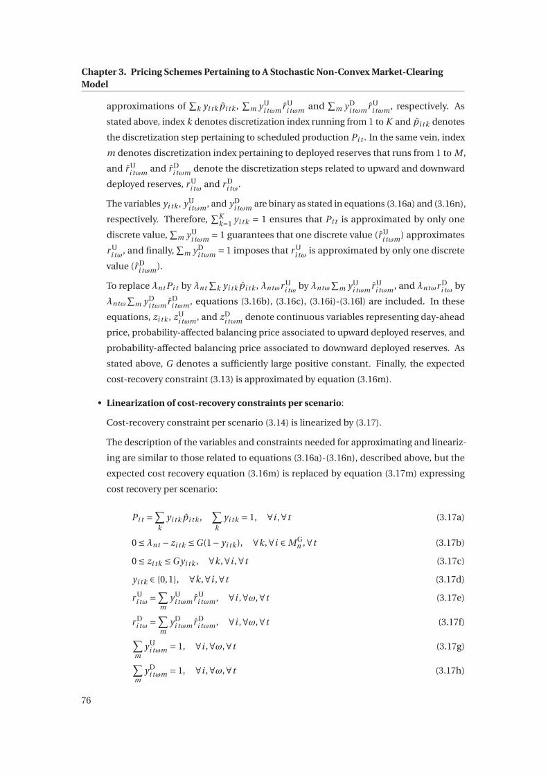
Chapter 3. Pricing Schemes Pertaining to A Stochastic Non-Convex Market-ClearingModel
approximations of∑
k yi tk pi tk ,∑
m yUi tωmr U
i tωm and∑
m yDi tωmr U
i tωm , respectively. As
stated above, index k denotes discretization index running from 1 to K and pi tk denotes
the discretization step pertaining to scheduled production Pi t . In the same vein, index
m denotes discretization index pertaining to deployed reserves that runs from 1 to M ,
and r Ui tωm and r D
i tωm denote the discretization steps related to upward and downward
deployed reserves, r Ui tω and r D
i tω.
The variables yi tk , yUi tωm , and yD
i tωm are binary as stated in equations (3.16a) and (3.16n),
respectively. Therefore,∑K
k=1 yi tk = 1 ensures that Pi t is approximated by only one
discrete value,∑
m yUi tωm = 1 guarantees that one discrete value (r U
i tωm) approximates
r Ui tω, and finally,
∑m yD
i tωm = 1 imposes that r Ui tω is approximated by only one discrete
value (r Di tωm).
To replace λnt Pi t by λnt∑
k yi tk pi tk , λntωr Ui tω by λntω
∑m yU
i tωmr Ui tωm , and λntωr D
i tω by
λntω∑
m yDi tωmr D
i tωm , equations (3.16b), (3.16c), (3.16i)-(3.16l) are included. In these
equations, zi tk , zUi tωm , and zD
i tωm denote continuous variables representing day-ahead
price, probability-affected balancing price associated to upward deployed reserves, and
probability-affected balancing price associated to downward deployed reserves. As
stated above, G denotes a sufficiently large positive constant. Finally, the expected
cost-recovery constraint (3.13) is approximated by equation (3.16m).
• Linearization of cost-recovery constraints per scenario:
Cost-recovery constraint per scenario (3.14) is linearized by (3.17).
The description of the variables and constraints needed for approximating and lineariz-
ing are similar to those related to equations (3.16a)-(3.16n), described above, but the
expected cost recovery equation (3.16m) is replaced by equation (3.17m) expressing
cost recovery per scenario:
Pi t =∑k
yi tk pi tk ,∑k
yi tk = 1, ∀i ,∀t (3.17a)
0 ≤λnt − zi tk ≤G(1− yi tk ), ∀k,∀i ∈ M Gn ,∀t (3.17b)
0 ≤ zi tk ≤G yi tk , ∀k,∀i ,∀t (3.17c)
yi tk ∈ {0,1}, ∀k,∀i ,∀t (3.17d)
r Ui tω =∑
myU
i tωmr Ui tωm , ∀i ,∀ω,∀t (3.17e)
r Di tω =∑
myD
i tωmr Di tωm , ∀i ,∀ω,∀t (3.17f)
∑m
yUi tωm = 1, ∀i ,∀ω,∀t (3.17g)
∑m
yDi tωm = 1, ∀i ,∀ω,∀t (3.17h)
76

3.6. Illustrative Example
0 ≤λnωt − zUi tωm ≤G(1− yU
i tωm), ∀m,∀i ∈ M Gn ,∀ω,∀t (3.17i)
0 ≤λnωt − zDi tωm ≤G(1− yD
i tωm), ∀m,∀i ∈ M Gn ,∀ω,∀t (3.17j)
0 ≤ zUi tωm ≤G yU
i tωm , ∀m,∀i ,∀t ,∀ω (3.17k)
0 ≤ zDi tωm ≤G yD
i tωm , ∀m,∀i ,∀t ,∀ω (3.17l)
0 ≤∑
t
(−Ci Pi t −C SU
i t +∑k
zi tk pi tk+ (3.17m)
∑m
(zUi tωmr U
i tωm − zDi tωmr D
i tωm)/πω−Ci t (r Ui tω− r D
i tω)
), ∀i ,∀ω
yUi tωm , yD
i tωm ∈ {0,1}, ∀m,∀i ,∀ω,∀t · (3.17n)
3.5.6 Complete Model
To summarize, primal-dual problem (3.11) with equations (3.15a)-(3.15e) results in prices
guaranteeing cost-recovery conditions at the day-ahead market, problem (3.11) with con-
straints (3.16a)-(3.16n) materializes prices ensuring cost-recovery conditions in expectation,
and finally this model with equations (3.17a)-(3.17n) achieves prices with the feature of cost-
recovery conditions per scenario.
We should note that the primal-dual problem (3.11) with cost-recovery constraints optimizes
over the primal variables (in set Ξp ) and the dual variables (in set Ξd ), as well as additional vari-
ables introduced in this section for linearization, i.e., Ξl = {zi tk , yi tk ,∀i ,∀t ,∀k; zUi tωm , yU
i tωm ,
zDi tωm , yD
i tωm ,∀i ,∀t ,∀ω,∀m}.
3.6 Illustrative Example
For the sake of illustration, in this section, we apply the proposed pricing approaches to a
simple system, and compare the market outcomes obtained from these approaches to those
from the conventional pricing method with uplift.
We reiterate that the prices from the conventional method are obtained by freezing binary
variables at their optimal value, which result from solving the primal problem (3.4), and
computing prices as dual variables of the corresponding LP problem [46].
3.6.1 Data
We consider a three-node system over a two-period time horizon. The system is shown in Fig.
3.1.
77
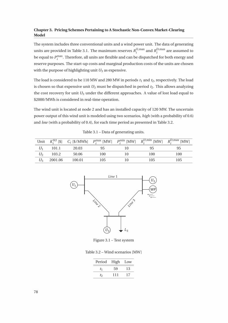
Chapter 3. Pricing Schemes Pertaining to A Stochastic Non-Convex Market-ClearingModel
The system includes three conventional units and a wind power unit. The data of generating
units are provided in Table 3.1. The maximum reserves RU,maxi and RD,max
i are assumed to
be equal to P maxi . Therefore, all units are flexible and can be dispatched for both energy and
reserve purposes. The start-up costs and marginal production costs of the units are chosen
with the purpose of highlighting unit U3 as expensive.
The load is considered to be 110 MW and 280 MW in periods t1 and t2, respectively. The load
is chosen so that expensive unit U3 must be dispatched in period t2. This allows analyzing
the cost recovery for unit U3 under the different approaches. A value of lost load equal to
$2000/MWh is considered in real-time operation.
The wind unit is located at node 2 and has an installed capacity of 120 MW. The uncertain
power output of this wind unit is modeled using two scenarios, high (with a probability of 0.6)
and low (with a probability of 0.4), for each time period as presented in Table 3.2.
Table 3.1 – Data of generating units.
Unit K SUi [$] Ci [$/MWh] P max
i [MW] P mini [MW] RU,min
i [MW] RD,maxi [MW]
U1 101.1 20.03 95 10 95 95
U2 103.2 50.06 100 10 100 100
U3 2001.06 100.01 105 10 105 105
WP𝑈 𝑈
𝑈 𝐿
𝐿𝑖𝑛𝑒 1
Figure 3.1 – Test system
Table 3.2 – Wind scenarios [MW]
Period High Low
t1 59 13
t2 111 17
78

3.6. Illustrative Example
Finally, line reactances and capacities are all equal to 0.13 p.u. and 500 MW, respectively. This
line capacity is sufficiently high to avoid congestion in any of the scenarios considered in order
to analyze solely the impact of uncertain wind production in this example.
3.6.2 Market Outcomes
We start discussing the results by providing quantities including the day-ahead scheduled
productions and the deployed reserves in real-time operation, as shown in Fig. 3.2.
U1 U2 U3 Wind0
50
Day−a
head
sche
dule
[MW
]
Period t1
U1 U2 U3 Wind0
50
100
Period t2
r1 r2 r3 spill−100−50
050
Dep
loye
dre
serv
esin
sce
nario
hi
gh [M
W]
r1 r2 r3 spill−100−50
050
r1 r2 r3 spill−50
0
50
Dep
loye
dre
serv
esin
sce
nario
lo
w [M
W]
r1 r2 r3 spill−50
0
50
U CR AR SR
Figure 3.2 – Scheduled productions and deployed reserves obtained from the conventionalmethod and the proposed pricing approaches.
Focusing on period t1, the different approaches result in similar day-ahead scheduled produc-
tions for all units. That is, all approaches allocate 41 MW to unit U1, 10 MW to unit U2 and 59
MW to wind unit, which is the wind power output in scenario High. If scenario High occurs in
real-time operation, there is no need to deploy reserves, and if scenario Low occurs, where the
wind power output is 13 MW, unit U1 is deployed 46 MW.
In period t2, the scheduled productions of unit U3 (the expensive unit) and wind unit differ
under the different approaches. The approach with day-ahead cost-recovery conditions
schedules unit U3 to produce up to its capacity generation, i.e., 105 MW, while allocating 16
MW to wind unit. In other words, this approach allocates the highest production to unit U3
and the lowest to wind unit comparing to the corresponding production levels from the other
approaches. To assess these differences, we look at their impacts on the prices obtained from
the different approaches.
Table 3.3 provides the day-ahead prices from the proposed approaches and from the conven-
tional approach. Since there is no congestion in any of the two scenarios considered, prices
79

Chapter 3. Pricing Schemes Pertaining to A Stochastic Non-Convex Market-ClearingModel
do not change across nodes.
The day-ahead prices are higher in period t2 than in period t1 due to a higher load in this
period (110 MW and 280 MW, respectively).
The approach with the day-ahead cost-recovery constraints results in the highest day-ahead
price, which is $119.06/MWh in period t2.
In the following, we elaborate on the impact of these prices on the unit profits.
Table 3.3 – Day-ahead prices [$/MWh]
method λt1 λt2
U 20.03 70.04
CR 33.84 119.06
AR 33.84 103.87
SR 33.84 103.47
Fig. 3.3 depicts the producer profits at the day-ahead market,∑
t
[Pi t (λnt −Ci )−C SU
i t
],∀i ,
and in expectation,∑
t
[Pi t (λnt −Ci )−C SU
i t +∑ωπω
((r U
i tω−r Di tω)(λntω/πω−Ci )
)],∀i , under the
different pricing approaches considered.
We should note that the profits obtained from the conventional method with uplift (black
bars) and without uplift (white bars) differ only for units incurring losses in the day-ahead
market, as uplift is paid only to these units.
Focusing on the performance of the conventional method in the day-ahead market and unit
U3, this unit earns 10×70.04 = $700.4 ($70.04/MWh is the marginal price at period t2) while
its total cost, including production and start-up costs, is 10×100.01+2001.06 = $3001.16.
Therefore, the profit of unit U3 resulting from the day-ahead market is $-2300.7. To prevent
unit U3 from incurring losses, the conventional method proposes to pay an uplift. We reiterate
that uplifts are paid only to those units incurring losses as a side-payment with the purpose of
reducing these losses to zero, and not to provide an extra profit. Since uplift takes actual losses
into account, it is computed based on the day-ahead scheduled productions and prices as
follows: |max{0,∑
t (ci −λnt )Pi t +C SUi t }| = |max{0,(100.01−70.04)10+2001.06}| = 2300.7. As
depicted at the top plot in Fig. 3.3, the day-ahead profit of unit U3 is zero under the method
with uplift (denoted by U) and negative under the method without uplift (denoted by Con).
The profits from the method with uplift (black bars) and without uplift (white bars) are the
same for units U1 and U2 as they do not incur losses, and therefore, do not receive uplifts.
80

3.6. Illustrative Example
This figure also shows that units U1 and U2 earn a higher day-ahead profit under the ap-
proaches with cost-recovery constraints than that under the method with uplift.
Focusing on unit U3, the approach with day-ahead cost-recovery constraints results in a
zero day-ahead profit. This is a better outcome in comparison to the negative day-ahead
profits resulting from the expected cost-recovery and per-scenario cost-recovery approaches.
However, the day-ahead cost-recovery approach does not prevent a negative profit in real-time
operation, as depicted at the bottom plot in Fig. 3.3.
Considering the expected profit (bottom plot in Fig. 3.3), the proposed approaches result in
higher expected profits for units U1 and U2 than those from the conventional method. We
reiterate that uplift is zero for these units, and hence, their expected profits are not affected by
uplifts, i.e., the white bars and black bars are the same for units U1 and U2. This observation
does not hold for unit U3. The approaches with average cost-recovery and per-scenario
cost-recovery constraints as well as the method with uplift result in a zero expected profit.
The total day-ahead profits (i.e., summation of the day-ahead profits of all units) obtained
from the approaches CR, AR, SR, as well as the method with uplift are $14,023.87, $9646.88,
$9707.19, and $5525.07, respectively. These outcomes are in line with the day-ahead prices
presented above: the day-ahead prices resulting from the approach with day-ahead cost
recovery are the highest, whereas those from the conventional method are the lowest.
U1 U2 U3
0
5
10
Day−a
head
prof
it [k
$]
U1 U2 U3
0
5
10
Exp
ecte
dpr
ofit
[k$]
Unit
Con U CR AR SR
Figure 3.3 – Day-ahead profit and expected profit
Table 3.4 provides the expected costs and the consumer payments, as well as the duality
gaps under the different pricing schemes. The methods with cost-recovery constraints in
expectation results in the same optimal expected cost as the primal clearing problem (i.e., the
optimal expected cost of the conventional method). The approaches with day-ahead cost-
recovery constraints and with cost-recovery constraints per scenario increase the expected
81

Chapter 3. Pricing Schemes Pertaining to A Stochastic Non-Convex Market-ClearingModel
cost by about 0.04% and 0.16%, respectively.
Under the approaches with cost-recovery conditions, the consumer payments are higher than
those from the method with uplift. The increases in consumer payments obtained from the
proposed approaches as a percentage of the consumer payment from the method with uplift
are also listed in this table. We should note that these large (unrealistic) differences are due to
the fact that this example does not represent a realistic case-study. Using a realistic case-study,
these differences get smaller.
Consumer payment consists of the day-ahead cost and the day-ahead profit. Noting com-
paratively small differences in the costs from the different approaches, the higher consumer
payments from the proposed approaches result from higher day-ahead profits caused by
higher day-ahead prices obtained from the proposed approaches.
The last row of Table 3.4 provides the social welfare gaps of the proposed pricing schemes. Also,
these gaps are listed as a percentage of the optimal expected cost of $13049.23. Although it
may seem that these gaps are not small enough in comparison with the optimal expected cost
obtained from the primal problem (3.4) (i.e., $13,044.5 in this example), one should notice that
the illustrative example presented does not represent a realistic case-study. It is provided for
the sake of clarity. Social welfare gaps obtained from applying the proposed pricing scheme to
realistic cases are provided in Section 3.7.5.
Table 3.4 – Expected cost, consumer payment, and duality gap in [$]
CR AR SR U
Expected cost 13054.09 13049.23 13069.95 13049.23
Consumer payment 33158.80 19280.86 23041.54 15159.05
(118.7%) (27.2%) (51.2%) –
Gap 2061.06 (15.8%) 1524.56 (11.7%) 1530.08 (11.7%) –
3.7 Case Studies
The case studies provided in this section aim to appraise the performance of the proposed pric-
ing schemes in a larger power system. To this aim, the outcomes of the proposed approaches
are benchmarked against the outputs of the conventional method with uplift.
82

3.7. Case Studies
3.7.1 Data
We apply the proposed approaches to a 24-node system based on the single-area IEEE Re-
liability Test System (RTS) [72]. To facilitate the analysis of the results, some of the original
characteristics of this test system are modified.
We consider the system to have 34 lines, 8 conventional generating units, 1 wind power unit,
and 5 loads.
The data of conventional generating units are provided in Table 3.5. We assume that hydro
unit U50 offers its energy at zero cost. The amount of reserve capacity that each generating
unit is willing to provide, either downward or upward, is assumed to be equal its production
capacity except from nuclear unit U400 that does not provide reserve.
The wind power unit, located at node 7, has an installed capacity of 600 MW. To generate wind
power scenarios, we use wind speed historical data from Austin, Texas, which are available
in the System Advisor Model (SAM) [2]. To obtain hourly wind power scenarios for 24 time
periods, we apply the power curve of a 2-MW Vestas V80/2000 wind turbine with a hub height
of 80 m. The power curve of this turbine model can be found in [16].
We should note that we built up the scenarios employing historical data without applying
scenario reduction techniques.
We consider 25 equi-probable scenarios for the wind power output in real-time operation.
Table 3.5 – Characteristics of the Generating Units
U76 U50 U155 U50 U197 U50 U400
Node 2 7 15, 18 15 21 22 23
P maxi [MW] 76 50 155 50 197 50 400
P mini [MW] 15 15 55 15 69 15 100
RU,maxi [MW] 76 50 155 50 197 50 0
RD,maxi [MW] 76 50 155 50 197 50 0
C SUi [$] 400 100 320 100 300 100 1000
Ci [$/MWh] 13.89 0 10.68 0 11.09 0 5.53
Table 3.6 provides the total demand over the 24 periods, while the demand locations and the
corresponding shares are provided in Table 3.7.
83

Chapter 3. Pricing Schemes Pertaining to A Stochastic Non-Convex Market-ClearingModel
Table 3.6 – Total demand in [MW]
t1 t2 t3 t4 t5 t6 t7 t8 t9 t10 t11 t12
441.1 481 482 483 490 1021.6 1132 1097 960.5 910.2 910 941.2
t13 t14 t15 t16 t17 t18 t19 t20 t21 t22 t23 t24
943 960 970 1031 1123 1130 1112 1101 998 930.1 780 440
Table 3.7 – Demand location
Demand D1 D2 D3 D4 D5
Node 1 4 13 14 20
Share % 33.5 18.9 14.9 16.2 16.5
3.7.2 Case I: No Network Congestion
In this case, the thermal limits of lines are considered to be high so that no congestion appears.
Therefore, the prices do not change across nodes
Since the driving factor of this chapter is the cost-recovery conditions of producers, we present
the market outcomes starting with producer profits.
U76 U50 U155 U50 U155 U197 U50 U4000
10
20
30
40
50
Unit
Day−a
head
Pro
fit [K
$]
ConCRARSR
Figure 3.4 – Day-ahead Profit (RTS no congestion case).
Fig. 3.4 shows the day-ahead profit obtained from the different approaches. Under the
conventional approach without uplift (white bars), units U76 and U197 incur losses (negative
day-ahead profits), and therefore, two uplifts totaling $1465 are required.
84

3.7. Case Studies
Using the proposed approaches, unit U197 has a positive day-ahead profit, and thus, does not
need uplift. However, unit U76 still incurs losses under the approaches with cost-recovery
constraints in expectation and per scenario, as these approaches do not enforce cost-recovery
conditions at the day-ahead market. The day-ahead profit of other units increases using the
proposed approaches. Among them, the day-ahead cost-recovery approach results in the
largest day-ahead profits. This is caused by the day-ahead prices, as described in the following.
2 4 6 8 10 12 14 16 18 20 22 245
10
15
20
25
Day−a
head
Pric
es [$
/MW
h]
Time periods
CRARSRCon
Figure 3.5 – Day-ahead prices at node 2 under different approaches (RTS no congestion case).
Fig. 3.5 depicts the day-ahead prices at node 2, where unit U76 is located, over the 24-hour
horizon. Since there is no congestion, the prices are the same at all nodes. Apart from period
t7 (morning peak) and period t18 (evening peak), the prices obtained from the approaches
with cost-recovery constraints are either equal or slightly higher than the prices obtained by
the conventional method. In period t18, the day-ahead prices obtained from the approaches
with cost-recovery constraints are the same and higher than the conventional marginal price.
However, a different behavior is observed in period t7. The approach with day-ahead cost-
recovery constraints results in a higher day-ahead price than those from the other approaches.
This consequently leads to a higher day-ahead profit from this approach, as observed in Fig.
3.4.
Fig. 3.6 shows the expected profit of the producers. In this figure, we distinguish the producer
profits with and without uplift by U and Con, respectively. One can observe that unit U76
cannot recover its expected cost under the prices obtained from the conventional method
without uplift (white bars). However, it attains a non-negative expected profit from the
approaches with cost-recovery constraints. Other units achieve higher profits under the
pricing approaches proposed than under the conventional method with uplift.
85

Chapter 3. Pricing Schemes Pertaining to A Stochastic Non-Convex Market-ClearingModel
U76 U50 U155 U50 U155 U197 U50 U4000
10
20
30
40
50E
xpec
ted
prof
it [K
$]
Unit
CRARSRUCon
Figure 3.6 – Expected Profit (RTS no congestion case).
Therefore, the proposed pricing approaches demonstrate the performance desired: the ap-
proach with day-ahead cost-recovery constraints guarantees non-negative day-ahead profit,
and the approaches with cost-recovery constraints in expectation and per scenario result
in non-negative expected profits. However, it is important to assess at what expenses these
outcomes are obtained. For this purpose, we provide the expected cost, consumer payment as
well as the duality gap in Table 3.8. The pricing methodologies with cost-recovery constraints
result in slightly higher expected cost than the one from the conventional method.
The approaches with cost-recovery conditions result in higher consumer payments than the
method with uplift. The increase in the consumer payments obtained from the proposed
approaches as a percentage of the consumer payment from the method with uplift is also
listed in Table 3.8. Note that consumer payment comprises day-ahead costs and day-ahead
profits. Higher day-ahead profits from the proposed approaches, described above, derive
higher consumer payments in these approaches as compared to those from the method with
uplift.
Finally, one can observe that the social welfare gaps in the last row are small in comparison
with the expected optimal social welfare from primal problem (3.4); they are of order of 0.3%
of the optimal expected cost of $127,066.
We should note that these differences are small, but also, they get smaller using a realistic
power system, as in a power system with a high penetration of renewable energy, gas units are
dominated technology among the conventional units due to their fast-ramping ability. Gas
units have small start-up costs and minimum production limits as compared to coal units.
86

3.7. Case Studies
Table 3.8 – Expected cost, consumer payment and duality gap for the RTS system [$] (RTS nocongestion case)
CR AR SR U
Expected cost 127,066 127,169 127,153 127,066
Consumers payment 2.42×10⁵ 2.34×10⁵ 2.38×10⁵ 2.17×10⁵
(11.5%) (7.8%) (9.7%) –
Gap 288.24 (0.2%) 384.80 (0.3%) 371.10 (0.3%) –
Therefore, we obtain a set of uniform prices under which cost-recovery conditions of producers
are guaranteed without a need of uplift at the expense of deviating about 0.3% from the optimal
social welfare.
For these simulation, we use CPLEX 12.1 under MATLAB on a computer Intel(R) Xeon(R) with
two processors clocking at 2.2 GHz and 512 GB of RAM. The sizes of the proposed models in
terms of number of variables and constraints as well as the computation time are provided in
Table 3.9. We elaborate on computation time in section 3.7.5.
Table 3.9 – Size of the proposed models
CR AR SR U
No. of continuous variables 93368 96968 96968 27600
No. of integer variables 1560 5160 5160 1176
No. of total variables 94928 102128 102128 28776
No. of constraints 95361 108561 108585 65384
Computation time (s) 22705 14231 1624 57
3.7.3 Impact of Minimum Up/Down Time Constraints
We have assumed start-up costs and minimum generation capacity as the only non-convexities
involved. However, other sources of non-convexity can be included without modeling dif-
ficulty, but different computational efforts. In this context, we investigate the impact of
minimum up/down time constraints in this section. We should note that these constraints
mostly pertain to old coal units and not to modern gas units. In a system with a large-scale
renewable penetration, it is expected that flexible gas units have a higher share of supply than
coal units. Therefore, the clearing model without these constraints represents a common
future power system, where a generation mix consists of renewable units and flexible units.
87

Chapter 3. Pricing Schemes Pertaining to A Stochastic Non-Convex Market-ClearingModel
The mathematical formulation of these constraints are provided in Appendix C.
We consider the minimum up time to be equal to the minimum down time for each con-
ventional unit, as provided in Table 3.10. A minimum up time of 3 hours is considered for
unit U76 in order to ensure that its respective minimum up time constraint is binding, and
therefore, the commitment of this unit is different from the commitment without considering
that constraint.
Table 3.11 provides the expected costs, the consumer payments, and the gaps obtained from
the different cost-recovery approaches under minimum up/down time constraints. The
increases in the consumer payments as a percentage of the consumer payment obtained from
the method with uplift are provided in Table 3.11. The gaps as a percentage of the optimal
expected cost of primal problem ($127,112) are also listed in this table.
Comparing these results to the outcomes from the formulation without minimum time con-
straints (Table 3.8), we conclude that the expected costs, the consumer payments, and the
gaps are similar. That is, the performance of the proposed approaches are not affected by
minimum up/down time constraints.
From the computational point of view, the approaches with day-ahead cost-recovery con-
straints and average cost-recovery constraints take the same computational efforts as the
simulations without minimum up/down time constraints. The computation time for the
approach with cost-recovery conditions per scenario, however, increases from 1624 s (for
the model without minimum up/down time constraints) to 4479 s (for the model with these
constraints).
Table 3.10 – Minimum Up/Down Time of Units
U76 U50 U155 U50 U197 U50 U400
Tmi n[h] 3 3 5 3 8 3 10
Table 3.11 – Expected cost, consumer payment and duality gap for the RTS system: No conges-tion case incorporating minimum Up/Down Time Constraints [$].
CR AR SR U
Expected cost 127,112 127,218 127,252 127,112
Consumers payment 2.37×10⁵ 2.34×10⁵ 2.39×10⁵ 2.17×10⁵
(9.2%) (7.8%) (10 %) –
Gap 275.5 (0.2%) 433.5 (0.3%) 471.3 (0.4%) –
88

3.7. Case Studies
3.7.4 Case II: Network Congestion
The purpose of this case is to explore the impact of congestion on day-ahead prices, and
consequently, on consumer payments.
To create network congestion, transmission limits of lines between node 2 and node 4, node 2
and node 6, node 3 and node 9, and node 6 to node 10 are set to be comparatively small (i.e.,
60 MW). As examples, the day-ahead prices at periods t18 and t21 are chosen for illustration
and depicted in Fig. 3.7. The prices from other periods also show the same behavior.
In period t18, the day-ahead prices obtained from the conventional method and the ap-
proaches with cost-recovery conditions are the same over all nodes apart from node 6, where
the average cost-recovery method results in a lower price. In period t21, the prices from the
conventional method and the cost-recovery approaches are almost equal over all nodes; there
are small price differences only at nodes 2, 4 and 6.
2 4 6 8 10 12 14 16 18 20 22 2410
11
12
13
Pric
e at
day−
ahea
d m
arke
t[$
/MW
h]
2 4 6 8 10 12 14 16 18 20 22 249
10
11
12
Pric
e at
day−
ahea
d m
arke
t[$
/MW
h]
Node
CR AR SR Con
Figure 3.7 – LMPs at t18 (up) and t21 (down) obtained by the different approaches.
Table 3.12 provides the expected costs, the consumer payments, and the duality gaps obtained
from the different approaches. The expected costs obtained from different approaches are
of the same order of magnitude. The consumer payments from the approaches with cost-
recovery constraints are of the same order of magnitude, and generally, about 3% higher than
that from the method with uplift. Similar to the non-congested case, the social welfare gaps
are small; these gaps are of order of 0.13% of the optimal expected cost ($170257).
89

Chapter 3. Pricing Schemes Pertaining to A Stochastic Non-Convex Market-ClearingModel
Table 3.12 – Expected cost, consumer payment and duality gap for the RTS system withcongestion [$].
CR AR SR U
Expected cost 170,257 170,271 170,273 170,257
Consumers payment 2.87×10⁵ 2.85×10⁵ 2.86×10⁵ 2.77×10⁵
(3.6%) (2.9%) (3.2%) –
Gap 211.58 (0.1%) 174.27 (0.1%) 230.91 (0.1%) –
3.7.5 Discussion on Social Welfare Gap and Computation Time
In this section, we elaborate on the computational aspects of the proposed models and the
relevance of the deviation from the expected optimal social welfare, i.e., the social welfare
gap. For this purpose, we simulate the proposed approaches using a number of different load
profiles for both no-congestion and congestion cases.
Outcomes show the same trend as those reported in Sections 3.7.2 and 3.7.4. That is, the
day-ahead prices obtained from the proposed approaches guarantee cost-recovery condi-
tions at the expense of an increase in the expected cost. The relevant metrics providing this
information are the expected cost and consumer payment, as described in the following.
1 2 3 4 5 6 70
0.2
0.4
Expected Cost
%
1 2 3 4 5 6 70
5
10Consumer Payment
Load profile
%
CRARSR
Figure 3.8 – Cost increase in percent, and consumer payment increase in percent for differentload profiles (RTS no congested case)
Fig. 3.8 shows the increase in the expected cost using the cost-recovery approaches as a
percentage of the optimal expected cost of primal problem (3.4), and the increase in consumer
payment obtained from the cost-recovery approaches as a percentage of the payment resulting
from the method with uplift. A similar trend is observed in case of congestion, as depicted in
90

3.7. Case Studies
Fig. 3.9. The increases in the expected cost are of order of less than 0.5%, and the increases in
the consumer payments are of order of less than 9%.
1 2 3 4 5 6 70
0.2
0.4Expected Cost
%
1 2 3 4 5 6 70
2
4
6
8Consumer Payment
Load profile
%
CRARSR
Figure 3.9 – Cost increase in percent, and consumer payment increase in percent for differentload profiles (RTS congestion case)
1 2 3 4 5 6 70
0.5
1Gap as a Percenatge of the Optimal Social Welfare from Primal Problem
%
1 2 3 4 5 6 70
0.2
0.4
0.6
Load profile
%
CRARSR
Non−congested Case
Congested Case
Figure 3.10 – Social welfare gaps as a percentage of the optimal expected cost obtained fromprimal problem 3.4 for different load profiles
The social welfare gaps as a percentage of the optimal expected cost obtained from primal
problem (3.4) for different load profiles are shown in Fig. 3.10. The gaps obtained from the
different proposed approaches are of the same order of magnitude, and small in comparison
with the optimal expected cost.
Referring to Table 3.9, the approach with day-ahead cost-recovery constraints requires a high
computation time. This can be partly explained by the small gap obtained from this approach
for all load profiles in the non-congested case and for most of the profiles in the congested case
91

Chapter 3. Pricing Schemes Pertaining to A Stochastic Non-Convex Market-ClearingModel
(see Fig. 3.10). Note, however, that for MILP models, there is no linear relationship between
the size of the problem and the required computation time. In other words, a smaller problem
(with smaller number of variables and constraints) may take longer to solve than a larger
problem.
The average computation time considering different load profiles for models CR, AR, and SR
are, respectively, 5473 s, 4964 s, and 4479 s, which are not significantly different. Note that the
computation burden may be considerably reduced by carefully adjusting the linearization of
the cost-recovery conditions. By doing this, computation requirements are expected to be not
much higher than those of a standard stochastic clearing model. We elaborate on the impact
of linearization steps on computation time in the next section.
3.7.6 Impact of Linearization Step
The impact of linearization steps on the problem outcomes is elaborated in this section.
On one hand, a smaller linearization step approximates more precisely the problem, but on
the other hand, significantly increases the dimension of the problem and its computational
burden.
Computational burden particularly matters when considering small linearization steps for the
deployed reserves in the approach with cost-recovery constraints in expectation and the ap-
proach with cost-recovery constraints per scenario. The reason is that the number of required
decision variables (yUi tωm , yD
i tωm , zUi tωm , and zD
i tωm , ∀i ,∀t ,∀ω,∀m), and constraints, (con-
straints (3.16i)-(3.16l) for the approach with average cost-recovery conditions, and constraints
(3.17i)-(3.17l) for the approach with per-scenario cost-recovery conditions) significantly in-
crease.
In the simulations, thus far presented, linearization steps of 5 MW and 19 MW have been
considered, respectively, for the day-ahead scheduled productions and the deployed reserves.
We next consider a linearization step of 2 MW for both the day-ahead productions and de-
ployed reserves (a drastic reduction) and provide the outcomes in Table 3.13. Comparing
these outcomes with those provided in Table 3.8 (with linearization steps of 5 MW and 19
MW), we conclude that this smaller linearization step results in very similar expected costs
(less than 0.03% differences), but smaller gaps for all proposed approaches. It also results in
smaller consumer payments for the approach with day-ahead cost-recovery constraints (2.5%
reduction) and the approach with average cost-recovery constraints (0.4% reduction), and the
same consumer payment for the approach with cost-recovery constraints per scenario.
From a computational point of view, the smaller linearization steps of 2 MW increase the
92

3.7. Case Studies
computation time from 14321 s to 19581 s for the approach with cost-recovery constraints in
expectation, and from 1624 s to 10983 s for the approach with cost-recovery constraints per
scenario. The computation time for the approach with day-ahead cost-recovery constraints
remains the same as the one for the linearization steps of 5 MW and 19 MW.
To summarize, a smaller linearization step leads to slightly more precise results at the expense
of higher computation time, while still the same conclusions are derived.
Table 3.13 – Expected cost, consumer payment and duality gap for the RTS system: no conges-tion case and linearization steps of 2MW for both schedules and deployed reserves.
CR AR SR
Expected cost 127055 127122 127131
Consumers payment 2.36×10⁵ 2.33×10⁵ 2.38×10⁵
Gap 282.8 347.6 359.9
3.7.7 Case Study Conclusion
We propose pricing approaches with cost-recovery conditions at the day-ahead, in expectation,
and per scenario for a stochastic non-convex clearing model.
Day-ahead prices obtained from the proposed approaches are higher than conventional
marginal prices in some periods. This, consequently, causes higher producer profits, and
therefore, higher consumer payments. However, the new prices eliminate the need of uplifts
and allow the market to fully rely on these new marginal prices. These conclusions are not
affected by network congestion, as well as by considering other sources of non-convexity such
as minimum up/down time constraints of units.
The increase in consumer payment varies from 3% to 9% of a payment derived from the
method with uplift considering different load profiles and network congestion.
From a social welfare point of view, the proposed approaches with cost-recovery features imply
deviating the least possible amount from the optimal value of the expected cost. The approach
with day-ahead cost-recovery constraints results in the same expected cost as the original
primal two-stage problem for the different load profiles considered. The other proposed
approaches also attain optimal expected costs close to the one of the primal problem. The
increases in expected costs are of order of 0.5% of the optimal expected cost. In the same
vein, the duality gaps are also small. Considering different load profiles, the duality gaps are of
order of 0.5% of the optimal social welfare.
93

Chapter 3. Pricing Schemes Pertaining to A Stochastic Non-Convex Market-ClearingModel
From the computational point of view, the models proposed have bi-linear terms, which need
to be linearized using integer variables. In this process, a smaller linearization step leads
to slightly more precise results at the expense of higher computation burden, but still the
same conclusions are derived. Generally, the models proposed are tractable and solvable in a
reasonable time using a MILP state-of-the-art solver.
3.8 Summary and Conclusion of the Chapter
Pricing schemes in non-convex electricity markets constitute an active area of research. Re-
cently, the growth of renewable generation and the possibility of using of stochastic clearing
models have added a new dimension to the traditional pricing problem: uncertainty.
This chapter proposes pricing methodologies in the presence of non-convexity and stochas-
ticity in electricity markets. The proposed approaches result in locational marginal prices
which guarantee cost-recovery conditions for producers, and therefore, eliminate a need for
uplifts. The prices obtained deviate in the least possible manner from conventional marginal
prices. This implies that a minimum deviation from the optimal value of social welfare is
also guaranteed. Moreover, the new prices preserve the short-term economic efficiency and
long-term cost recovery properties of marginal prices.
The proposed pricing methods may be of interest for regulators to replace the existing pricing
methods that require uplifts.
94

4 Economic Impact of Flexible De-
mands
4.1 Introduction
In the previous chapters, we have focused on market-clearing models as tools facilitating a
large-scale integration of renewable generation. In this chapter, we change the view from the
role of tools to the role of market players, particularly demands.
A high penetration of renewable generation requires a system with sufficient flexibility. Flexi-
bility is the operational ability of a generating unit or a demand to be scheduled by the system
operator with some degree of freedom. The operational flexibility of demands and units allows
the system operator to adjust them in order to absorb renewable production to the largest
extent at a minimum cost. While flexibility of a generating unit is reflected in its ramping
capability, demand flexibility includes the ability to move consumption across periods, and to
change the consumption level per period. Hence, a system with a large amount of renewable
generation needs to promote demand flexibility and building fast-ramping units. This implies
that a common future power generation mix may consist of comparatively cheap renewable
units and comparatively expensive fast-ramping units.
Given that the driving factors behind marginal prices are the production costs of units, a swing
between high marginal prices (due to high production costs of fast-ramping units) and low
marginal prices (due to small production costs of renewable units) seems likely. But also, high
demand flexibility may alter energy prices such that what is known nowadays as peak and
off-peak prices may fade by demand flexibility, as it basically shifts energy consumption from
peak periods to off-peak periods.
The interaction between energy prices and flexible demands is complex. On one hand, de-
mand flexibility is recognized to be beneficial to the system as a whole since such flexibility
facilitates the integration of renewable generation with a reduced operation cost, but on the
95

Chapter 4. Economic Impact of Flexible Demands
other hand, shifting demands from peak periods to off-peak periods may influence prices to
an extent that affects the willingness of demands to be flexible.
Therefore, in a power system with a high penetration of cheap renewable production and
expensive fast-ramping units, a legitimate question is whether being flexible is advantageous
for demands.
To address this question, this chapter analyzes the operational and economic impacts of
demand flexibility, particularly demand revenues.
Note that the contribution of demands in providing flexibility to assist the integration of
renewable generation ([44] and [1]) from the system point of view is discussed in [39], [75],
and [74]. However, analyses focusing on the economic impacts of demand flexibility are not
common in the literature, particularly the impact of different degrees of demand flexibility on
day-ahead prices.
4.2 Approach
We investigate the economic consequences resulting from flexible demand actions in a market
involving a significant amount of cheap renewable power production and expensive fast-
ramping units. To this aim, we use a two-stage stochastic clearing model, similar to the
model introduced in Chapter 2. However, this model is carefully adapted to consider demand
flexibility.
We should note that the use of a two-stage model is solely for the sake of convenience. A
multi-stage model comprising a number of intra-day markets in addition to the day-ahead
market and real-time one can be considered without difficulties. Note that this does not
change the outcome of the analyses in this chapter.
An actual system exhibiting the properties described above is the one in mainland Spain, a
system mostly based on gas and wind units. The energy prices may swing between high prices
driven by comparatively expensive gas units and low prices driven by comparatively cheap
wind units. Inspired by this system, we consider a power system with a generation mix of
wind and gas units for our analyses and investigate the impact of demand flexibility in such a
system by following the steps below:
• We consider flexible demands with a certain minimum daily energy consumption, and
the ability to move their consumptions across time periods.
• We use a two-stage model to obtain the day-ahead market outcomes including sched-
96

4.3. Assumptions
uled power production of units, scheduled power consumptions of demands, and
day-ahead prices.
• The prices are obtained using the prevalent price scheme in industry [46] that is de-
scribed as the conventional pricing approach in Chapter 3. We should note that if pricing
schemes other than the one adopted [46] are used, e.g., a convex-hull pricing [24], the
problem of concern remains the same, and therefore, the choice of pricing scheme is
not particularly relevant.
• Next, we consider demands to be inflexible with the same daily energy consumptions as
those considered for flexible demands, and we obtain the day-ahead market outcomes.
• Finally, the results of the case with flexible demands are compared to the outcomes
obtained from inflexible demands.
4.3 Assumptions
Before elaborating on the mathematical formulation of the clearing model with flexible de-
mands, we list below the assumptions considered for the sake of simplicity and convenience.
• A generation mix of wind units and gas units are considered for our analyses. Wind
power output is considered to be the only source of uncertainty.
• Wind power output is represented by a number of scenarios. These scenarios are
built using historical wind production data as samples without applying any scenario
generation/reduction techniques.
• The wind producers are assumed to offer their production at a comparatively small cost.
• For simplicity, the cost functions of generating units and utility functions of flexible
demands are assumed to be linear.
• The cost of deploying reserve is the cost of energy production if the source for reserve
deployment is a unit, and if the source is a flexible demand, the utility of demand is the
cost of deploying reserve.
the utility of a flexible demand if the source is a demand.
• The stochastic clearing model co-optimizes energy and reserve deployment without
explicit reserve offers in the day-ahead market. Units and flexible demands can specify
the reserve limits (MW) that they are willing to provide, and hence, we give them the
opportunity of reserve deployment for a profit.
97

Chapter 4. Economic Impact of Flexible Demands
• A linear representation of the transmission network is considered through a dc load flow
model where losses are neglected.
• We do not consider security criteria, such as n-1, to focus on the analyses of wind
uncertainty.
• The non-convexities considered are solely those due to non-zero minimum power
outputs of conventional units, start-up costs, and binary unit-commitment variables.
Taking into account other source of non-convexities, such as shut-down costs and
minimum up/down time constraints, is straightforward.
4.4 Model Description: Two-Stage Stochastic Clearing with Flexible
Demands
The decision-making sequence of the two-stage model is described in Chapter 2. Hence, we
do not repeat the description of variables and constraints. However, the two-stage model still
needs to be adapted to consider flexible demands.
In the following, we first list variables and constraints pertaining to demand flexibility, and
next, we provide the mathematical description of the two-stage model with flexible demands
followed by a brief description of the constraints.
4.4.1 Flexible Demands as Decision Variables
Similar to generating units, flexible demands are scheduled in the day-ahead market before
wind power output is realized. These flexible demands can also react to actual wind power
output in real-time operation by deploying reserves.
Therefore, the day-ahead demand schedules are first-stage variables, while flexible demands
in term of providing reserve deployments are second-stage variables. We define actual loads
as second-stage variables that result from the day-ahead demand schedules and real-time
deployments, i.e., d j tω = D j t +d Dj tω−d U
j tω.
Therefore, the following variables are considered in addition to the set of variables described in
Section 2.4.2, i.e., Ξ= {C SUi t ,ui t ,Pi t ,∀i ,∀t ;Wqt ,∀q,∀t ;θnt ,∀n,∀t ;r U
i tω,r Di tω,∀i ,∀t ,∀ω; wspill
qtω ,
∀q,∀t ,∀ω;θntω,∀n,∀t ,∀ω;Lshedj tω ∀ j ,∀t ,∀ω}:
• Load scheduled for each flexible demand in each period at the day-ahead market (D j t ,
[MW]).
98

4.4. Model Description: Two-Stage Stochastic Clearing with Flexible Demands
• Deployed up-reserve by each flexible demand in each period and each scenario in
real-time operation (d Uj tω, [MW]).
• Deployed down-reserve by each flexible demand in each period and each scenario in
real-time operation (d Dj tω, [MW]).
• Actual load consumed by each flexible demand in each period and each scenario in
real-time operation (d j tω, [MW]).
• Final power output of each generating unit in each period and each scenario in real-time
operation (p j tω, [MW]).
Objective Function
In the presence of flexible demands, the objective function to be maximize is the expected
social welfare, and it includes the following terms:
• The day-ahead cost that includes the start-up cost and production costs of conventional
units, the production cost of wind units, and the utility of flexible demands over all
periods of the market horizon:
NT∑t=1
( NG∑i=1
(C SUi t +Ci Pi t )+
NQ∑q=1
CqWqt −NL∑j=1
U j t D j t)
(4.1)
• The expected balancing cost that results from the deployed reserves by conventional
units and flexible demands, and involuntary load shedding in real-time operation:
NT∑t=1
NΩ∑ω=1
πω
[ NG∑i=1
Ci (r Ui tω− r D
i tω)+NQ∑
q=1Cq (W RT
qtω−Wq −wspillqtω )
+NL∑j=1
V LOLj t Lshed
j tω −U j t (d Dj tω−d U
j tω)]
(4.2)
Thus, the expected social welfare is:
NT∑t=1
NG∑i=1
−C SUi t −
NΩ∑ω=1
πω
[ NT∑t=1
( NG∑i=1
Ci pi tω+NQ∑
q=1Cq (W RT
qtω−wspillqtω )+
NL∑j=1
(V LOLj t Lshed
j tω −U j t d j tω))]
(4.3)
where pi tω = Pi t + r Ui tω− r D
i tω and d j tω = D j t +d Dj tω−d U
j tω.
We should note that demand utilities are equivalent to bid prices, submitted by demands to
99

Chapter 4. Economic Impact of Flexible Demands
the market, and thus, the model proposed incorporates demand bids in form of U j t d j tω, i.e.,
U j t (D j t +d Dj tω−d U
j tω).
4.4.2 Constraints pertinent to Demand Flexibility
We define demand flexibility to be the ability of demands to move their consumption across
periods, and to change their consumption level per period. That is, demands provide a
consumption range to the system operator within which they can vary according to the
preference of the operator (to benefit the system), but they have a certain energy consumption
that must be respected by the system operator.
In this context, we introduce the following new constraints pertaining to flexible demands in
the day-ahead market as well as in real-time operation:
Day-ahead Market Constraints
Considering the power balance equation in the day-ahead market expressed in (2.5), the
inflexible demand L j t changes to flexible demand D j t of which schedule is determined in the
market:
∑i∈M G
n
Pi t +∑
q∈M Qn
Wqt −∑
j∈M Ln
D j t −∑
r∈Λn
Bnr (θnt −θr t ) = 0,∀n,∀t (4.4)
The day-ahead demand schedules are enforced to be within the minimum and maximum
limits in each period:
Dminj t ≤ D j t ≤ Dmax
j t ,∀ j ,∀t (4.5)
Similar to the ramping limits of units, demands have pick-up and drop-down rate limits.
The pick-up/drop-down rates represent how a flexible load can increase or decrease its con-
sumption. The day-ahead demand schedules are enforced to respect these limits in each
period:
RD j ≤ D j t −D j ,t−1 ≤ RU j ,∀ j ,∀t (4.6)
Real-time Operation Constraints
Considering the power balance equation in real-time operation expressed in (2.35), apart from
100

4.4. Model Description: Two-Stage Stochastic Clearing with Flexible Demands
units, flexible demands also provide deployed reserves:
∑i∈M G
n
(r Ui tω− r D
i tω)+ ∑q∈M Q
n
(W RTqtω−Wqt −wspill
qtω )− ∑j∈M L
n
(d Dj tω−d U
j tω+Lshedj tω )
+ ∑r∈Λn
Bnr (θnt −θntω−θr t +θr tω) = 0,∀n,∀t ,∀ω (4.7)
The actual load, resulting from the reserve deployment provided by the flexible demands, is
enforced to be within the demand limits in real-time operation for each scenario and each
time period:
Dminj t ≤ d j tω ≤ Dmax
j t ,∀ j ,∀t ,∀ω (4.8)
The pick-up/drop-down rate limits of flexible demand j shall be respected in real-time opera-
tion for each scenario and each time period:
RD j ≤ d j tω−d j ,t−1,ω ≤ RU j ,∀ j ,∀t ,∀ω (4.9)
The total consumption of actual demand d j tω over all periods shall respect the minimum
daily energy consumption of flexible demand j , denoted by E j . This is enforced by constraint
(4.10):
E j ≤NT∑t=1
d j tω,∀ j ,∀ω (4.10)
The deployed reserves are limited between zero and the available amount of reserves offered
by flexible demands:
0 ≤ d Dj tω ≤ RD,max
j t ,∀ j ,∀t ,∀ω (4.11)
0 ≤ d Uj tω ≤ RU,max
j t ,∀ j ,∀t ,∀ω (4.12)
4.4.3 Mathematical Model
The MILP market-clearing model including flexible demands is as follows:
MaximizeΞD
101

Chapter 4. Economic Impact of Flexible Demands
NT∑t=1
NG∑i=1
−C SUi t −
NΩ∑ω=1
πω
[ NT∑t=1
( NG∑i=1
Ci pi tω+NQ∑
q=1Cq (W RT
qtω−wspillqtω )+
NL∑j=1
(V LOLj t Lshed
j tω −U j t d j tω))]
(4.13a)
subject to
First-stage constraints:∑i∈M G
n
Pi t +∑
q∈M Qn
Wqt −∑
j∈M Ln
D j t −∑
r∈Λn
Bnr (θnt −θr t ) = 0,∀n,∀t (4.13b)
K SUi (ui t −ui ,t−1) ≤C SU
i t ,∀i ,∀t (4.13c)
ui t ∈ {0,1},∀i ,∀t (4.13d)
ui t P mini ≤ Pi t ≤ ui t P max
i ,∀i ,∀t (4.13e)
Dminj t ≤ D j t ≤ Dmax
j t ,∀ j ,∀t (4.13f)
Wqt ≤W maxq ,∀q,∀t (4.13g)
RDi ≤ Pi t −Pi ,t−1 ≤ RUi ,∀i ,∀t (4.13h)
RD j ≤ D j t −D j ,t−1 ≤ RU j ,∀ j ,∀t (4.13i)
θ1t = 0,∀t (4.13j)
Second-stage constraints:∑i∈M G
n
(r Ui tω− r D
i tω)+ ∑q∈M Q
n
(W RTqtω−Wqt −w spill
qtω )− ∑j∈M L
n
(d Dj tω−d U
j tω+Lshedj tω )
+ ∑r∈Λn
Bnr (θnt −θntω−θr t +θr tω) = 0,∀n,∀t ,∀ω (4.13k)
pi tω = Pi t + r Ui tω− r D
i tω (4.13l)
d j tω = D j t +d Dj tω−d U
j tω (4.13m)
ui t P mini ≤ pi tω ≤ ui t P max
i ,∀i ,∀t ,∀ω (4.13n)
Dminj t ≤ d j tω ≤ Dmax
j t ,∀ j ,∀t ,∀ω (4.13o)
RDi ≤ pi tω−pi ,t−1,ω ≤ RUi ,∀i ,∀t ,∀ω (4.13p)
RD j ≤ d j tω−d j ,t−1,ω ≤ RU j ,∀ j ,∀t ,∀ω (4.13q)
− f maxnr ≤ Bnr (θntω−θr tω) ≤ f max
nr ,∀n,∀r ∈Λn ,∀t ,∀ω (4.13r)
E j ≤NT∑t=1
d j tω,∀ j ,∀ω (4.13s)
r Ui tω ≤ RU,max
i t ,∀i ,∀t ,∀ω (4.13t)
r Di tω ≤ RD,max
i t ,∀i ,∀t ,∀ω (4.13u)
d Dj tω ≤ RD,max
j t ,∀ j ,∀t ,∀ω (4.13v)
d Uj tω ≤ RU,max
j t ,∀ j ,∀t ,∀ω (4.13w)
102

4.4. Model Description: Two-Stage Stochastic Clearing with Flexible Demands
Lshedj tω ≤ d j tω,∀ j ,∀t ,∀ω (4.13x)
wspillqtω ≤W RT
qtω,∀q,∀t ,∀ω (4.13y)
θ1tω = 0,∀t ,∀ω (4.13z)
0 ≤ Pi t ,C SUi t ,∀i ,∀t , 0 ≤Wqt ,∀q,∀t
0 ≤ r Ui tω,r D
i tω,∀i ,∀t ,∀ω, 0 ≤ w spillqtω ,∀q,∀t ,∀ω
0 ≤ Lshedj tω ,d U
j tω,d Dj tω,∀ j ,∀t ,∀ω (4.13aa)
whereΞD = {C SUi t ,Pi t ,∀i ,∀t ;Wqt ,∀q,∀t ;D j t ,∀ j ,∀t ;θnt ,∀n,∀t ; pi tω,r U
i tω,r Di tω,∀i ,∀t ,∀ω;d j tω,
d Uj tω,d D
j tω,Lshedj tω ,∀ j ,∀t ,∀ω; wspill
qtω ,∀q,∀t ,∀ω;θntω,∀n,∀t ,∀ω} is the set of optimization vari-
ables.
The problem (4.13) maximizes the expected social welfare (4.13a) considering the day-ahead
constraints (4.13b)-(4.13j), the real-time operation constraints (4.13k)-(4.13z), and variable
declarations expressed in (4.13aa).
A brief description of the constraints is as follows. Constraint (4.13b) represents the power
balance in the day-ahead market, where scheduled power production of units and scheduled
loads of flexible demands are determined. The start-up costs are modeled by equation (4.13c),
which depend on the on/off status of each generating unit via binary variable ui t in constraint
(4.13d). The limits of production of conventional units, flexible demands, and wind production
in the day-ahead market are represented by constraints (4.13e), (4.13f) and (4.13g), respectively.
Constraint (4.13h) enforces the ramping limits of generating units. Similarly, constraint (4.13i)
enforces the pick-up/drop-down rate limits of flexible demands in the day-ahead market.
Constraint (4.13j) establishes that node 1 is the reference node in the day-ahead market.
Constraint (4.13k) stands for power balance in real-time operation, where actual wind power
output is compensated by deploying reserves provided by conventional units and flexible
demands, as well as (in rare cases) load shedding. The power output of unit i during period
t and scenario ω is described by equation (4.13l), and the actual load for flexible demand
j in period t and scenario ω by equation (4.13m). The reserve deployment provided by the
conventional units shall respect the generation limits, and the reserve deployment provided
by the flexible demands must be within the demand limits in real-time operation. These limits
are considered in constraints (4.13n) and (4.13o), respectively. Constraint (4.13p) represents
the ramping limits of generating units, and constraint (4.13q) represents the pick-up/drop-
down rate limits of flexible demands in real-time operation. Constraint (4.13r) enforces that
the line flows stay within the transmission capacity limits at real-time operation. Note that
enforcing this constraint is not generally required in the day-ahead market. The day-ahead
schedules can violate these limits as long as actual power flows are still within the transmission
103
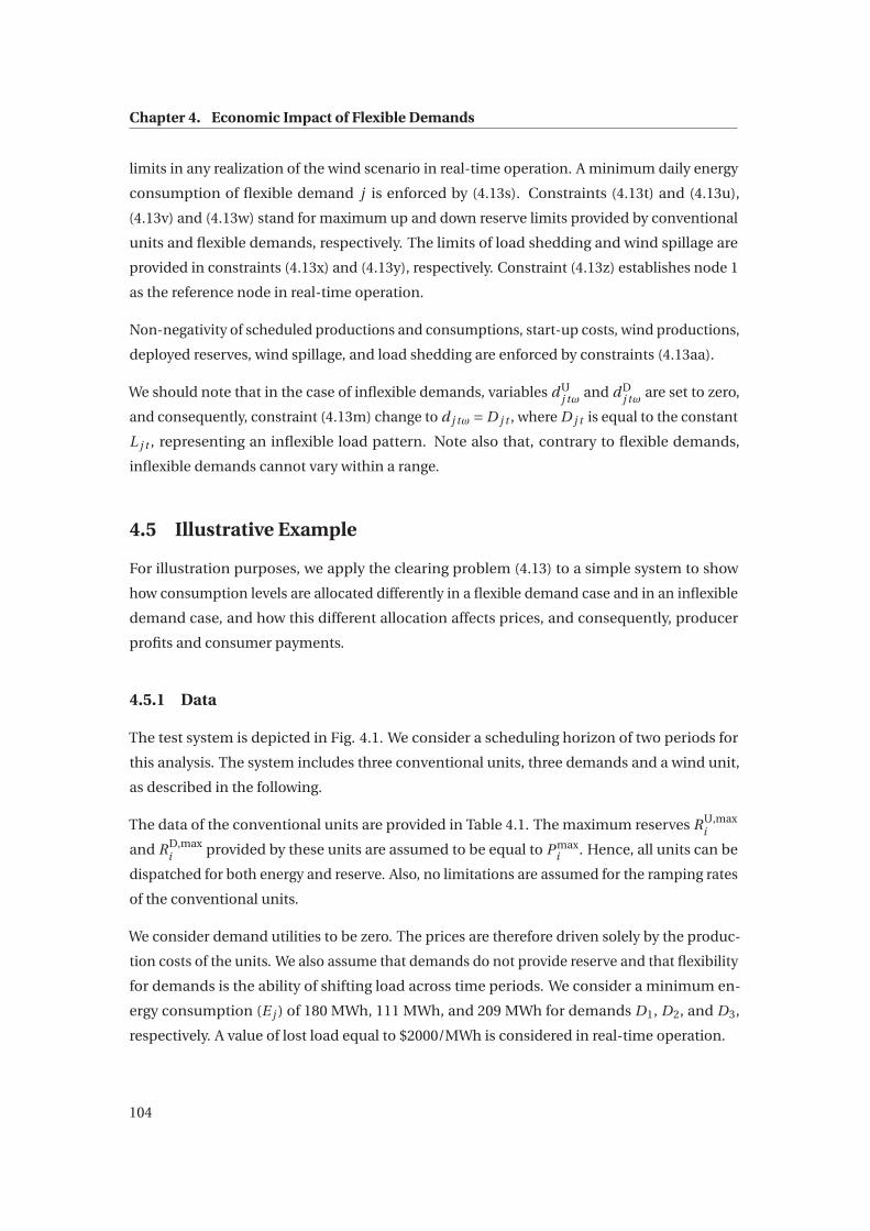
Chapter 4. Economic Impact of Flexible Demands
limits in any realization of the wind scenario in real-time operation. A minimum daily energy
consumption of flexible demand j is enforced by (4.13s). Constraints (4.13t) and (4.13u),
(4.13v) and (4.13w) stand for maximum up and down reserve limits provided by conventional
units and flexible demands, respectively. The limits of load shedding and wind spillage are
provided in constraints (4.13x) and (4.13y), respectively. Constraint (4.13z) establishes node 1
as the reference node in real-time operation.
Non-negativity of scheduled productions and consumptions, start-up costs, wind productions,
deployed reserves, wind spillage, and load shedding are enforced by constraints (4.13aa).
We should note that in the case of inflexible demands, variables d Uj tω and d D
j tω are set to zero,
and consequently, constraint (4.13m) change to d j tω = D j t , where D j t is equal to the constant
L j t , representing an inflexible load pattern. Note also that, contrary to flexible demands,
inflexible demands cannot vary within a range.
4.5 Illustrative Example
For illustration purposes, we apply the clearing problem (4.13) to a simple system to show
how consumption levels are allocated differently in a flexible demand case and in an inflexible
demand case, and how this different allocation affects prices, and consequently, producer
profits and consumer payments.
4.5.1 Data
The test system is depicted in Fig. 4.1. We consider a scheduling horizon of two periods for
this analysis. The system includes three conventional units, three demands and a wind unit,
as described in the following.
The data of the conventional units are provided in Table 4.1. The maximum reserves RU,maxi
and RD,maxi provided by these units are assumed to be equal to P max
i . Hence, all units can be
dispatched for both energy and reserve. Also, no limitations are assumed for the ramping rates
of the conventional units.
We consider demand utilities to be zero. The prices are therefore driven solely by the produc-
tion costs of the units. We also assume that demands do not provide reserve and that flexibility
for demands is the ability of shifting load across time periods. We consider a minimum en-
ergy consumption (E j ) of 180 MWh, 111 MWh, and 209 MWh for demands D1, D2, and D3,
respectively. A value of lost load equal to $2000/MWh is considered in real-time operation.
104

4.5. Illustrative Example
The wind power plant, at node 2, has an installed capacity of 300 MW. A small production cost
of $0.3/MWh is assumed for this unit. Two equi-probable scenarios are used to model the
wind power output uncertainty for each time period, as provided in Table 4.2. We should note
that period t1 represents a period with a high wind power production while at period t2 the
wind power output significantly decreases.
All line reactances are equal to 0.13 p.u. and all line capacities are set to be high enough to
avoid congestion.
WP𝑈 𝑈
𝑈 𝐷
𝐿𝑖𝑛𝑒 1𝐷 𝐷
Figure 4.1 – Test system
Table 4.1 – Data of generating units.
Unit K SUi [$] Ci [$/MWh] P max
i [MW] P mini [MW] RU,max
i [MW] RD,maxi [MW]
U1 300.01 10.03 95 15 95 95
U2 102.2 30.02 100 10 100 100
U3 101.2 31.01 105 5 105 105
Table 4.2 – Wind scenarios (W RTqtω)[MW]
Period scenario ω1 scenario ω2
t1 283 299
t2 10 13
105

Chapter 4. Economic Impact of Flexible Demands
4.5.2 Market Outcomes
Below, we present the results, including day-ahead schedules and day-ahead prices, for two
cases, one with flexible demands and other with inflexible demands.
Fig. 4.2 shows the day-ahead scheduled production (upper plots) and scheduled demands
(bottom plots) for the cases described.
In the case with inflexible demands, the consumption is assumed to be fixed to 283 MW in
period t1 and to 217 MW in period t2 (total 500 MW).
In this allocation, none of the conventional units is scheduled in period t1 (the load is covered
solely by the wind unit), whereas all of them are scheduled in period t2. On the other hand,
in the case with flexibility, demand is moved from period t2 to period t1 so that a larger load
share (378 MW from 500 MW) is allocated to period t1 and a smaller one (122 MW from 500
MW) to period t2. Note that this is the outcome that we aim to obtain in order to be able to
explore the impact of flexible demands on marginal prices.
U1 U2 U3 Wind0
100
200
300DA Scheduled Units at t1
MW
U1 U2 U3 Wind0
100
200 DA Scheduled Units at t2
MW
D1 D2 D30
50
100
150
MW
D1 D2 D30
50
100
MW
Flex. Demand Inflex. Demand
DA ScheduledDemands at t1
DA ScheduledDemands at t2
Figure 4.2 – Day-ahead scheduled units and demands - illustrative example
Table 4.3 provides the day-ahead prices λt and the probability-removed balancing prices
λtω/πω per scenario. Since there is no congestion in any of the scenarios considered, electricity
prices do not change across nodes.
As mentioned in the previous chapters, these prices are obtained as dual variables of power
balance equations after setting the binary unit-commitment variables to their optimal values
[46].
In period t1, the price from the inelastic demand case is the lowest, whereas it is the highest in
period t2. This is due to the commitment decisions: since none of the conventional units is
106

4.5. Illustrative Example
committed in period t1, the corresponding prices obtained are solely driven by the small cost
of the wind unit. However, in period t2 all conventional units are online and the corresponding
prices are driven by the marginal production cost of unit U3. Under flexible demands, the shift
of demands from period t2 to period t1 turns unit U1 on in period t1, which results in a higher
price ($10.03/MWh) than that of the inflexible demand case ($0.3/MWh).
Table 4.3 – Day-ahead and probability-removed balancing prices ($/MWh)
Flexible demand Inflexible demand
t1 t2 t1 t2
λ 10.03 30.02 0.3 31.01
λω1 /πω1 10.03 30.02 0.3 31.01
λω2 /πω2 10.03 30.02 0.3 31.01
Therefore, demand flexibility results in higher prices in valley and slightly lower prices in peak.
Given these schedules and prices, Table 4.4 provides the day-ahead profit, expected profit,
day-ahead cost, expected cost, consumer payment, and uplift for the different cases.
Table 4.4 – Market outcomes of three-node system
Flexible demand Inflexible demand
Unit DA Exp. DA Exp.
Profit Profit Profit Profit
($) ($) ($) ($)
U1 -0.16 1599.04 14.69 1693.09
U2 -102.20 -102.20 -92.30 -3.20
U3 0.00 0.00 -101.20 -101.20
Wind 5801.84 5801.84 5742.77 5742.77
Total 5699.48 7298.68 5563.96 7331.46
DA Exp. DA Exp.
Cost ($) 1754.30 2783.70 1250.10 4872.20
Consumer Payment ($) Consumer Payment ($)
7453.80 6814.10
Uplift ($) Uplift ($)
102.36 193.50
The inflexible demand case results in a higher expected cost and a lower day-ahead cost than
those from the case with flexibility. The comparatively lower day-ahead cost of the inflexible
demand case is due to a higher amount of wind power scheduled in the day-ahead market.
However, this requires a high expected balancing cost of deployed reserves, and eventually,
107

Chapter 4. Economic Impact of Flexible Demands
leads to a higher total expected cost than that of the case with flexibility.
This observation confirms that demand flexibility is beneficial to the system, as it decreases
the operation cost.
Focusing on unit profits, the inflexible demand case results in a smaller total day-ahead profit
(i.e., $5563.96 vs $5699.48), but a larger total expected profit than those from the flexible
demand case. The smaller total day-ahead profit is due to the low prices (i.e., $0.3/MWh) that
are driven by the off status of the conventional units in period t1, and a larger total expected
profit results from high prices (i.e., $31/MWh) obtained in period t2.
Note that under the day-ahead prices obtained, units U1 and U2 cannot recover their produc-
tion costs in the flexible demand case, as well as units U2 and U3 in the inflexible demand
case. These losses disappear or decrease, if the respective units are deployed at the operation
stage, such as unit U1 in the flexible demand case and unit U2 in the inflexible demand case.
Adopting the common practice of uplifts, these side-payments are provided for both cases.
Finally, the consumer payment, which is the summation of the day-ahead cost and total
day-ahead profit, is smaller under the inflexible demands than that under flexible demands.
Note that the flexible demand case results in a smaller day-ahead cost, but a higher total
day-ahead profit. The latter causes a higher consumer payment under this case than that of
the inflexible demand case. In other words, demand flexibility results in prices that increase
unit profits, and consequently, the demand payments.
Therefore, although demand flexibility is beneficial to the system as a whole, it may result in
prices not beneficial for the flexible demands.
4.6 Case Studies
In this section, we present two case studies: one without network congestion and without
ramping limits of units, and another with both network congestion and ramping limits of
units.
Similar to the illustrative example and for simplicity, the utility of demands is considered to be
zero. Therefore, the marginal prices are linked to the production costs of units.
In other words, we explore a situation where demands support the system operator with a full
scale flexibility free of charge, and compare the operational and economic outcomes to the
case with inflexible demands.
108

4.6. Case Studies
4.6.1 Data
The test system is a modified version of the 24-node system based on the single-area IEEE RTS
[72] including a generation mix of expensive fast-ramping units and one wind unit to facilitate
the analyses of the results.
The system considered has 34 lines, 8 conventional units, and 1 wind power unit. The data
of conventional units are provided in Table 4.5. Note that apart from hydro units U50, the
rest of the units have relatively high production costs as compared to the cheap wind unit.
As previously mentioned, such a generation mix is motivated by the case of mainland Spain,
whose generation mix is dominated by gas and wind units. Considering this generation mix, we
note that gas units (CCGTs) are generally not subject to minimum up/down time constraints.
Therefore, these constraints are not considered. We assume that the limit of reserve capacity
is equal to the capacity of each conventional unit.
Table 4.5 – Characteristics of the Generating Units
U90 U50 U155 U76 U197
Node 2 7,15 10,18 16 21,22
P maxi [MW] 90 50 20 76 197
P mini [MW] 25 15 12 15.2 69
K SUi [$] 400 100 400 400 300
Ci [$/MWh] 19.67 0.2 10.68 11.89 18.09
RU,maxi [MW] 90 50 20 76 197
RD,maxi [MW] 90 50 20 76 197
Table 4.6 provides demand data including their location and minimum energy consumption
E j .
The wind power unit, located at node 7, has an installed capacity of 1000 MW. To generate wind
power scenarios, we use wind speed historical data from Austin, Texas, which are available
in the System Advisor Model (SAM) [2]. To obtain hourly wind power scenarios for 24 time
periods, we apply the power curve of a 2-MW Vestas V80/2000 wind turbine with a hub height
of 80 m. The power curve of this turbine model can be found in [16].
We should note that we built up the scenarios employing historical data without applying
scenario reduction techniques.
We consider 30 equi-probable scenarios for the wind power output in real-time operation.
109
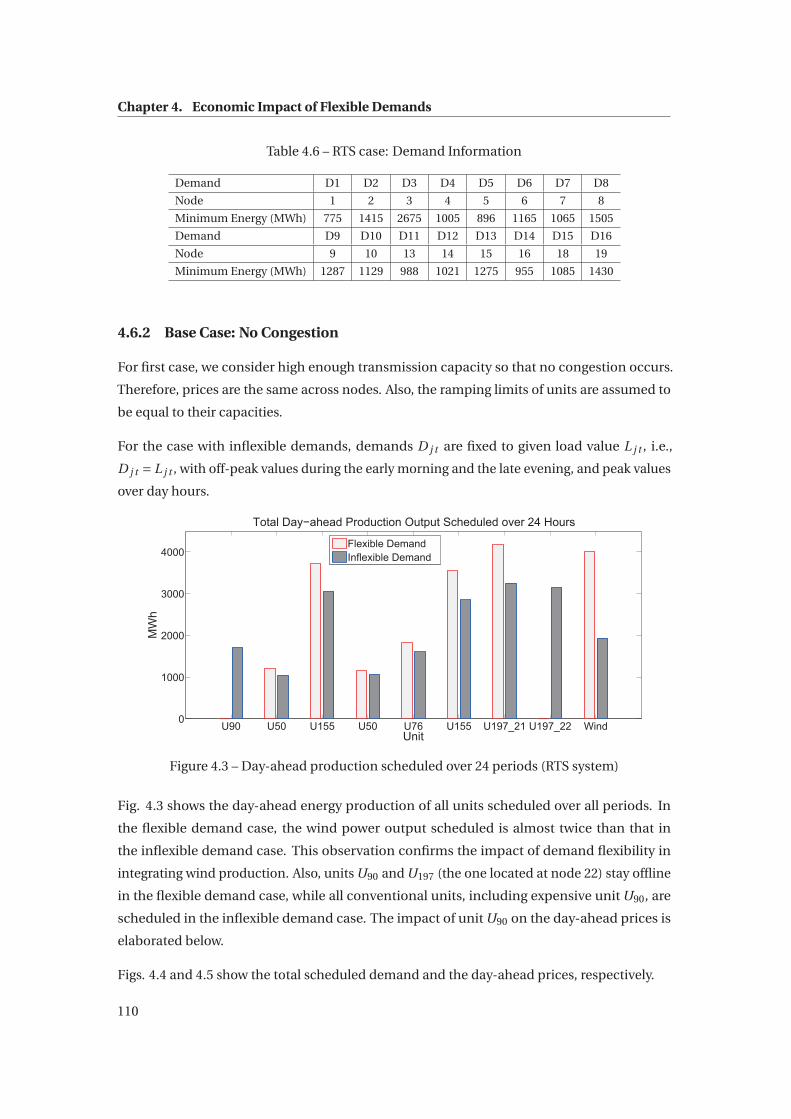
Chapter 4. Economic Impact of Flexible Demands
Table 4.6 – RTS case: Demand Information
Demand D1 D2 D3 D4 D5 D6 D7 D8
Node 1 2 3 4 5 6 7 8
Minimum Energy (MWh) 775 1415 2675 1005 896 1165 1065 1505
Demand D9 D10 D11 D12 D13 D14 D15 D16
Node 9 10 13 14 15 16 18 19
Minimum Energy (MWh) 1287 1129 988 1021 1275 955 1085 1430
4.6.2 Base Case: No Congestion
For first case, we consider high enough transmission capacity so that no congestion occurs.
Therefore, prices are the same across nodes. Also, the ramping limits of units are assumed to
be equal to their capacities.
For the case with inflexible demands, demands D j t are fixed to given load value L j t , i.e.,
D j t = L j t , with off-peak values during the early morning and the late evening, and peak values
over day hours.
U90 U50 U155 U50 U76 U155 U197_21 U197_22 Wind0
1000
2000
3000
4000
Unit
MW
h
Total Day−ahead Production Output Scheduled over 24 Hours
Flexible DemandInflexible Demand
Figure 4.3 – Day-ahead production scheduled over 24 periods (RTS system)
Fig. 4.3 shows the day-ahead energy production of all units scheduled over all periods. In
the flexible demand case, the wind power output scheduled is almost twice than that in
the inflexible demand case. This observation confirms the impact of demand flexibility in
integrating wind production. Also, units U90 and U197 (the one located at node 22) stay offline
in the flexible demand case, while all conventional units, including expensive unit U90, are
scheduled in the inflexible demand case. The impact of unit U90 on the day-ahead prices is
elaborated below.
Figs. 4.4 and 4.5 show the total scheduled demand and the day-ahead prices, respectively.
110

4.6. Case Studies
In the case with inflexible demands (blue and squares), during periods t1 − t4 demands are
relatively small and can be supplied solely by wind generation. In the mid-day hours, demand
grows while wind generation decreases. Therefore, to cover the demands, other units are
required. Focusing on the outcome from flexible demands (red and circles), demands are
shifted to periods t1 − t5 and periods t20 − t24 which are periods with cheap wind generation.
Correspondingly, the day-ahead prices have a different pattern for these cases: in the case
with inflexible demands, in periods t1 − t3 and t22 − t24 the day-ahead prices are derived from
the small production cost of wind unit, and therefore, are very low. With the load increase
starting at period t4, the prices increase until period t20, when the load decreases. In the
flexible demand case, the day-ahead prices are relatively high for all periods, however, still
smaller than the peak price of the inflexible demand case. They are overall high since demands
are shifted to low-demand periods (night hours). Increasing the demands in these periods
that now require both wind and conventional units (except from expensive unit U90) results in
overall high prices. Due to the off status of unit U90, the peak price of the case with flexible
demands is smaller than that of the inflexible demand case.
5 10 15 20200
400
600
800
1000
1200Load Pattern
time period
MW
Inflex. DemandFlex. Demand
Figure 4.4 – Demand pattern obtained from the flexible and inflexible demand cases (RTSsystem)
Table 4.7 provides details regarding day-ahead profits, expected profits, day-ahead costs,
expected costs (i.e., the total of day-ahead cost and balancing cost1 ), consumer payments,
uplifts, and total day-ahead scheduled demand resulting from the two case: flexible and
inflexible demands.
For the same amount of scheduled demand (i.e., 19,671 MWh), moving from the case with
inflexible demands to the case with flexibility, a cost saving of 24% is obtained in the day-ahead
1The day-ahead cost, the expected balancing cost, and the total expected cost are formulated in (4.1), (4.2),(4.3), respecively.
111
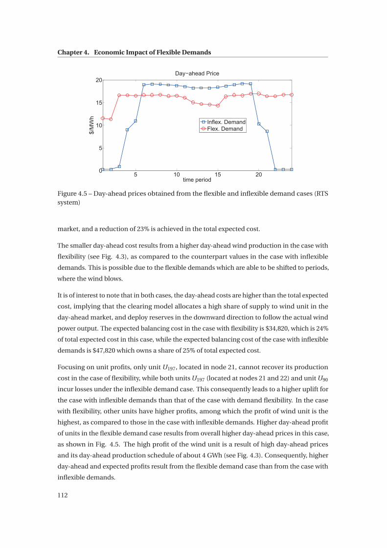
Chapter 4. Economic Impact of Flexible Demands
5 10 15 200
5
10
15
20Day−ahead Price
time period
$/M
Wh
Inflex. DemandFlex. Demand
Figure 4.5 – Day-ahead prices obtained from the flexible and inflexible demand cases (RTSsystem)
market, and a reduction of 23% is achieved in the total expected cost.
The smaller day-ahead cost results from a higher day-ahead wind production in the case with
flexibility (see Fig. 4.3), as compared to the counterpart values in the case with inflexible
demands. This is possible due to the flexible demands which are able to be shifted to periods,
where the wind blows.
It is of interest to note that in both cases, the day-ahead costs are higher than the total expected
cost, implying that the clearing model allocates a high share of supply to wind unit in the
day-ahead market, and deploy reserves in the downward direction to follow the actual wind
power output. The expected balancing cost in the case with flexibility is $34,820, which is 24%
of total expected cost in this case, while the expected balancing cost of the case with inflexible
demands is $47,820 which owns a share of 25% of total expected cost.
Focusing on unit profits, only unit U197, located in node 21, cannot recover its production
cost in the case of flexibility, while both units U197 (located at nodes 21 and 22) and unit U90
incur losses under the inflexible demand case. This consequently leads to a higher uplift for
the case with inflexible demands than that of the case with demand flexibility. In the case
with flexibility, other units have higher profits, among which the profit of wind unit is the
highest, as compared to those in the case with inflexible demands. Higher day-ahead profit
of units in the flexible demand case results from overall higher day-ahead prices in this case,
as shown in Fig. 4.5. The high profit of the wind unit is a result of high day-ahead prices
and its day-ahead production schedule of about 4 GWh (see Fig. 4.3). Consequently, higher
day-ahead and expected profits result from the flexible demand case than from the case with
inflexible demands.
112

4.6. Case Studies
Table 4.7 – Economic Outcomes (base case - RTS system)
Flexible Inflexible
demand demand
Unit DA Exp. DA Exp.
Profit Profit Profit Profit
($) ($) ($) ($)
U90 0.00 0.00 -8672.29 -2697.86
U50 17691.48 17698.02 13310.71 14015.00
U155 18744.00 19343.47 13672.96 15189.82
U50 17146.79 17698.02 13955.38 14015.00
U76 6779.69 7406.56 3388.50 6055.38
U155 17740.75 19343.46 13358.34 15282.41
U197n21 -8163.73 -2309.13 -4619.08 -1555.64
U197n22 0.00 0.00 -4179.50 -1555.64
Wind 60924.56 60924.56 7341.70 7341.70
Total 130863.54 140104.95 47556.73 66090.18
DA Exp. DA Exp.
Cost ($) 180420.00 145600.00 236780.00 188960.00
Consumer Payment ($) Consumer Payment ($)
311280.00 284340.00
Uplift ($) Uplift ($)
8163.70 17471.00
Total DA Demand Total DA Demand
(MWh) (MWh)
19671.00 19671.00
Therefore, the case with flexibility results in a smaller day-ahead cost and a smaller uplift,
but a higher total day-ahead profit which leads to 9.5% increase in consumer payment, as
compared to those from the case with inflexible demands.
This observation shows an inherent conflict in incorporating demand flexibility into an elec-
tricity market: on one hand, the system benefits from the reduced operation cost caused by
demand flexibility, but on the other hand, the resulting prices increases the demand expenses.
Thus, demands might be better off being inflexible.
4.6.3 Impact of Ramping Limits and Congestion
In this section, we consider that the ramping capability of each unit is half of its capacity. That
is, reduced flexibility is provided by the conventional units to the system as compared to the
base case, i.e., the previous case. Also, in order to create congestion, we consider reduced
transmission capacity for the lines connecting node 2 to 1, to 4, and to 6, node 4 to 9, node 5 to
113

Chapter 4. Economic Impact of Flexible Demands
10 (i.e., line limits of 50 MW), and node 17 to 18, and to 22 (i.e., line limits of 137MW and 179
MW, respectively). With this consideration, congestion appears mainly in peak periods.
5 10 15 200
5
10
15
20
25Day−ahead Price at Node 5
time
$/M
Wh
Inflex. DemandFlex. Demand
Figure 4.6 – The day-ahead prices at node 5 over different periods (ramping limits and conges-tion case)
As an example of the day-ahead prices obtained, Fig. 4.6 shows the prices at node 5 over the
24-hour study horizon. Similar to the trend observed in the case without congestion, the
prices from the flexible demand case are higher over the off-peak periods and lower over the
peak-periods with respect to the prices from the case with inflexible demands.
2 4 6 8 10 12 14 16 18 20 22 2416
16.5
17
17.5
18
18.5
19
19.5
Day−ahead Price at t19
Node
$/M
Wh
Inflex. DemandFlex. Demand
Figure 4.7 – RTS case study with congestion: nodal day-ahead prices in period t19
As an example of the nodal prices (i.e., prices across the nodes), the day-ahead prices in period
t19 are shown in Fig. 4.7. The nodal prices from the inflexible case are higher than those
from the flexible demand case in this period. This observation is also valid for the other peak
periods, when price differentiation across nodes appears. Note that congestion does not occur
114
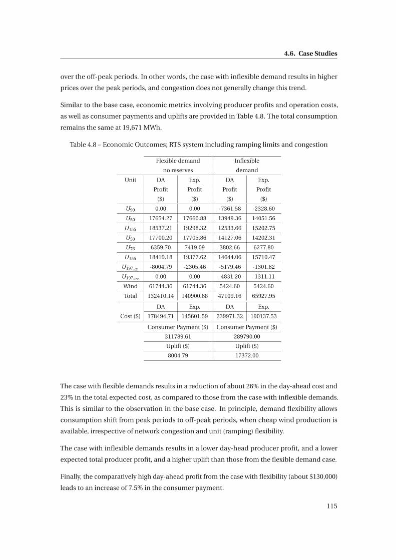
4.6. Case Studies
over the off-peak periods. In other words, the case with inflexible demand results in higher
prices over the peak periods, and congestion does not generally change this trend.
Similar to the base case, economic metrics involving producer profits and operation costs,
as well as consumer payments and uplifts are provided in Table 4.8. The total consumption
remains the same at 19,671 MWh.
Table 4.8 – Economic Outcomes; RTS system including ramping limits and congestion
Flexible demand Inflexible
no reserves demand
Unit DA Exp. DA Exp.
Profit Profit Profit Profit
($) ($) ($) ($)
U90 0.00 0.00 -7361.58 -2328.60
U50 17654.27 17660.88 13949.36 14051.56
U155 18537.21 19298.32 12533.66 15202.75
U50 17700.20 17705.86 14127.06 14202.31
U76 6359.70 7419.09 3802.66 6277.80
U155 18419.18 19377.62 14644.06 15710.47
U197n21 -8004.79 -2305.46 -5179.46 -1301.82
U197n22 0.00 0.00 -4831.20 -1311.11
Wind 61744.36 61744.36 5424.60 5424.60
Total 132410.14 140900.68 47109.16 65927.95
DA Exp. DA Exp.
Cost ($) 178494.71 145601.59 239971.32 190137.53
Consumer Payment ($) Consumer Payment ($)
311789.61 289790.00
Uplift ($) Uplift ($)
8004.79 17372.00
The case with flexible demands results in a reduction of about 26% in the day-ahead cost and
23% in the total expected cost, as compared to those from the case with inflexible demands.
This is similar to the observation in the base case. In principle, demand flexibility allows
consumption shift from peak periods to off-peak periods, when cheap wind production is
available, irrespective of network congestion and unit (ramping) flexibility.
The case with inflexible demands results in a lower day-head producer profit, and a lower
expected total producer profit, and a higher uplift than those from the flexible demand case.
Finally, the comparatively high day-ahead profit from the case with flexibility (about $130,000)
leads to an increase of 7.5% in the consumer payment.
115

Chapter 4. Economic Impact of Flexible Demands
Therefore, congestion and ramping limits of the conventional units do not change the conclu-
sions from the previous case, of which the most important one is that demands incur higher
expenses under the flexible demand case.
4.6.4 Case Study Conclusions
To get insights about the impact of demand flexibility, we compare two cases: one with highly
flexible demands in term of their ability to shift consumption across periods in the day-ahead
market without considering the demand ability of reserve provision for real-time deployment;
and the case with inflexible demands including inelastic demands following a traditional
consumption pattern with peak consumption in day hours and off-peak consumption in night
hours. The common feature of the two cases is that demands have the same total energy
consumption over the entire clearing horizon. Therefore, we are able to explore producers and
consumers expenses for the same amount of energy consumption. Based on the observations
in these case studies, we conclude the followings:
1. Demand flexibility is beneficial to the system, as it shifts consumption from day hours
to night hours, when cheap wind production is available. In other words, demand
flexibility adapts its consumption pattern to the production pattern of the wind unit.
Specifically, the scheduled production of the wind unit (i.e., the contribution of wind
production in energy supply) is almost twice in the case with flexibility. This leads to
a cost reduction of about 25%, as compared to the cost obtained from the case with
inflexible demands.
2. Due to the notable shift in consumption in the case with demand flexibility, a price
shift occurs: the prices from the flexible demand case are comparatively higher over
the off-peak periods and comparatively lower over the peak-periods with respect to the
prices from the case with inflexible demands. Network congestion and ramping limits
of the conventional units do not change these conclusions.
3. Higher off-peak prices result in a higher consumer payment in the flexible demand case
than that of the case with inflexible demands. The increase in consumer payment is 9%
in the base case and 7.5% in the case with congestion and limited ramping capability.
4. The observations from the case studies show an inherent conflict in incorporating
demand flexibility to an electricity market: on one hand, the system benefits from
the reduced operation cost caused by demand flexibility, but on the other hand, the
resulting prices increases the demand expenses. Thus, demands might be better off
being inflexible.
116

4.7. Summary and Conclusion of the Chapter
4.7 Summary and Conclusion of the Chapter
This chapter is devoted to analyze the economic consequences resulting from the actions of
flexible demands in a common future market consisting of a significant amount of renew-
able power production with comparatively low marginal cost and fast-ramping units with
comparatively high marginal cost, such as combined-cycle gas turbines.
On one hand, demand flexibility (the ability of some demands to move load from peak periods
to off-peak periods) is beneficial for the system as a whole since it decreases the expected
operation cost, but on the other hand, demand flexibility can result in price increases that
in turn increase demand expenses. Therefore, demands might be better off being inflexible
in systems with a generation mix dominated by comparatively cheap renewable units and
comparatively expensive fast-ramping units.
We should note that if pricing schemes other than the one adopted [46] are used, e.g., a convex-
hull pricing [24], the conclusions derived in our study are likely to remain valid provided that
the final prices do not deviate significantly from marginal prices.
We should also note that the use of a stochastic clearing model is for the purpose of obtaining
optimal outcomes in a market with a high penetration of renewable generation, and the choice
of clearing model, i.e., a deterministic or a stochastic one, does not change the conclusion
above.
The observations in this chapter call for new settlement approaches seeking to encourage
demand flexibility.
117


5 Two-Stage Stochastic Clearing Model
for the Reserve Market
5.1 Introduction
The system operator is responsible to ensure system security in power systems. A mechanism
to do so is reserve; in real-time operation, there is a need to compensate mismatches between
supply and demand in order to preserve the power balance in the system. For this purpose,
reserves are scheduled in a market prior to real time to be eventually deployed in real-time
operation. The structure of this market (e.g., gate closure, type of offers, etc.) depends on the
market organization, i.e., a centralized market organization and a decentralized one.
In a centralized market organization, such as electricity markets in the US, reserves are sched-
uled in the day-ahead market co-optimizing energy and reserves (this is similar to the clearing
models in Chapter 2), whereas in a decentralized market organization, such as electricity
markets in Europe, reserves are procured in reserve markets separately from energy markets.
In a centralized market, the system operator and market operator are generally the same entity.
However, a decentralized market separates energy transactions and system operations to a
large extent; the former is done by the market operator, whereas the latter is the responsibility
of the Transmission System Operator (TSO) [3].
The common practice in many European countries, as examples of the decentralized market
organization, is first to determine fixed amounts of reserves (of different types) using technical
(security) criteria, and then, to procure them in reserve markets. We challenge this practice as it
decouples technical criteria from market aspects, which may result in economic inefficiencies.
The particular focus of this chapter is the reserve market in Switzerland, as an example of
a decentralized market organization. We use two-stage stochastic clearing models to show
the advantages of our proposed model with respect to deterministic one, not only through
simulated case studies, but also through the outcomes of the actual implementation of the
119

Chapter 5. Two-Stage Stochastic Clearing Model for the Reserve Market
proposed two-stage clearing model.
The lay-out of this chapter is as follows. We first describe the Swiss reserve market in Section
5.2. Next, the decision-making process and scenarios are described in Sections 5.3 and 5.4,
respectively. Section 5.5 provides the assumptions that we use to model the reserve market.
Section 5.6 provides the mathematical descriptions of the proposed risk-neutral two-stage
stochastic model (in Section 5.6.1), of the proposed risk-averse counterpart (in Section 5.6.2),
and of a common deterministic model (in Section 5.6.3). Also, we formulate how to obtain
a perfect information solution as well as the actual cost of the two-stage model in Section
5.6.4. The proposed models are showcased through real cases from the Swiss reserve market
in Section 5.7. Finally, relevant remarks are concluded in Section 5.8.
5.2 The Swiss Reserve Market
In this section, we briefly describe the Swiss reserve market that is similar to those of other
countries in continental Europe.
5.2.1 Technical Description of Reserves in Europe
According to European Network of Transmission System Operators for Electricity (ENTSO-E)
definition, reserves are categorized as primary, secondary, and tertiary [47]. 1
Primary reserves react to frequency deviations in the interconnected Continental Europe
irrespective of the location of the contingencies. The corresponding amount is determined by
ENTSO-E and shared among all involved countries on an annual basis. Secondary reserves
automatically react to power imbalances within a time varying from a few seconds to several
minutes (e.g., load fluctuations). Finally, tertiary reserves are manually deployed to replace
secondary reserves [56, 34] if any power mismatch with a time duration more than several
minutes occurs (e.g., a constant (load) forecast error lasting more than 15 minute or an outage
of a power plant). In other words, secondary reserves compensate for spontaneous power
imbalances lasting a few to several seconds, while along with secondary reserves, tertiary
reserves are deployed to cover overall power mismatches lasting more than several minutes.
Therefore, secondary reserves are continuously in use, and hence, tertiary reserves cannot
be deployed without already-deployed secondary reserves. Fig. 5.1 illustrates the reaction
1In Guideline Electricity Balancing, reserves are called frequency containment reserves (FCR), frequencyrestoration reserves (FRR) and replacement reserves (RR) [13]. Also, frequency restoration reserves are categorizedinto automatic frequency restoration reserves (aFRR) and manual frequency restoration reserves (mFRR). The FCRand aFRR stand for primary and secondary reserves, respectively, while the mFRR is interpreted to be fast tertiaryreserves and the RR is considered as slow tertiary reserves.
120
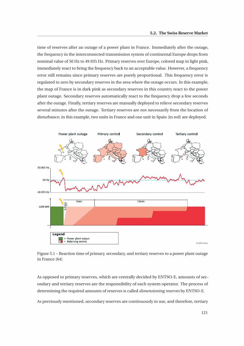
5.2. The Swiss Reserve Market
time of reserves after an outage of a power plant in France. Immediately after the outage,
the frequency in the interconnected transmission system of continental Europe drops from
nominal value of 50 Hz to 49.935 Hz. Primary reserves over Europe, colored map in light pink,
immediately react to bring the frequency back to an acceptable value. However, a frequency
error still remains since primary reserves are purely proportional. This frequency error is
regulated to zero by secondary reserves in the area where the outage occurs. In this example,
the map of France is in dark pink as secondary reserves in this country react to the power
plant outage. Secondary reserves automatically react to the frequency drop a few seconds
after the outage. Finally, tertiary reserves are manually deployed to relieve secondary reserves
several minutes after the outage. Tertiary reserves are not necessarily from the location of
disturbance; in this example, two units in France and one unit in Spain (in red) are deployed.
Figure 5.1 – Reaction time of primary, secondary, and tertiary reserves to a power plant outagein France [64]
As opposed to primary reserves, which are centrally decided by ENTSO-E, amounts of sec-
ondary and tertiary reserves are the responsibility of each system operator. The process of
determining the required amounts of reserves is called dimensioning reserves by ENTSO-E.
As previously mentioned, secondary reserves are continuously in use, and therefore, tertiary
121

Chapter 5. Two-Stage Stochastic Clearing Model for the Reserve Market
reserves cannot be deployed without considering already-deployed secondary reserves. There-
fore, two types of reserves are categorized for the reserve dimensioning process: secondary
and overall reserves. Overall reserves represent the total of secondary and tertiary reserves.
The system operator first determines the necessary amounts of secondary reserves and overall
reserves. The required amount of tertiary reserves is then obtained by subtracting the amount
of secondary reserves from the amount of overall reserves.
We should note that since determining the amount of primary reserves is the responsibility of
ENTSO-E, and not the TSOs, it is not consider in this chapter.
5.2.2 Reserve Dimensioning Criteria
In Switzerland, the dimensioning criteria that determine the required amount of reserves
include a probabilistic criterion and a deterministic one, as described in the following.
Probability Criterion:
The probability criterion states that the amount of reserves must be determined such that
power mismatches are regulated to zero with a probability of 99.8%. This implies that the
power balance in the system cannot be violated more than 0.2% of all hours over a year.
Therefore, the reserve amount R is determined by the 99.8% quantile of the power imbalance
distribution as expressed in inequality (5.1):
P(Δp ≤ R) ≥ 99.8% (5.1)
which is equivalent to:
P(Δp > R) ≤ 0.2% (5.2)
Inequality (5.2) describes the probability that a certain power deviation (Δp) exceeds a certain
quantity (R). This is translated to the probability that a certain amount of reserves (R) cannot
cover a certain power deviation. In other words, inequality (5.2) enforces that the probability
of the deficit of reserve (i.e., reserve deficit probability) must be equal to or smaller than 0.2%.
Given that there are two types of reserves (i.e., secondary and tertiary reserves), the probability
criterion is translated into the following. The portion of time over a year that secondary
reserves are not sufficient to cover spontaneous power mismatches and that the total of
secondary and tertiary reserves are not enough to cover power mismatches cannot exceed
122
5.2. The Swiss Reserve Market
0.2%. Therefore, inequality (5.2) is recast to:
P(Δps,+ > Rs,up)+P(Δps,− > Rs,dn)+P(Δpo,+ > Ro,up)+P(Δpo,− > Ro,dn) ≤ 0.2% (5.3)
where Δps,+, Δps,−, Δpo,+, Δpo,− denote positive spontaneous power imbalance, negative
spontaneous power imbalance, positive overall power imbalance, and negative overall power
imbalance, respectively. Positive spontaneous power imbalances denote power mismatches
resulting from situations where consumption exceeds generation within durations of order of
seconds. Therefore, upward secondary reserves Rs,up are deployed to keep the system power
balance. Negative spontaneous power imbalances represent power mismatches resulting
from situations where generation exceeds consumption within durations of order of seconds.
Thus, downward secondary reserves Rs,dn are deployed to keep the system power balance.
Positive overall power imbalances represent power mismatches resulting from situations
where consumption exceeds generation within durations of order of minutes. Therefore,
upward overall reserves Ro,up are deployed to keep the system power balance. Negative overall
power imbalances denote power mismatches resulting from situations where generation
exceeds consumption within durations of order of minutes. Thus, downward overall reserves
Ro,dn are deployed to keep the system power balance.
To evaluate the deficit probability, the system operator identifies the factors driving power
imbalances and their corresponding probability functions. These factors include load oscilla-
tions, load forecast errors, forecast errors of renewable generation, outages of power plants,
etc. We should note that some of these factors drive spontaneous power imbalances such as
load oscillations, while some others have a more permanent impact, such as outages of power
plants.
The Swiss TSO, Swissgrid, does not have a database with detailed information on the indi-
vidual factors deriving power imbalances. The available data only involves measurements
of Area Control Error (ACE) [34] 2 and deployed secondary and tertiary reserves. Therefore,
spontaneous power imbalances are calculated by adding the deployed secondary reserves
to the ACE measurements, and the overall power imbalances are computed by adding the
deployed secondary and tertiary reserves to the measurements of the ACE using the historical
data over a year.
Next, these datasets are used to statistically derive the corresponding cumulative distribution
functions. The advantage of using cumulative distribution functions is that these functions
easily describe the relationship between the deficit probability and the reserves.
2ACE is defined as the difference between scheduled power production and actual power within a control areaon the power grid, taking frequency bias into account
123

Chapter 5. Two-Stage Stochastic Clearing Model for the Reserve Market
Fig. 5.2 shows the cumulative distribution functions of power imbalances in the Swiss power
system in 2013. The larger the imbalance is, the smaller its probability is. Spontaneous power
imbalances (in blue) determine the amount of secondary reserves while overall imbalances
(in red) determine the amount of overall reserves.
−400 −300 −200 −100 0 100 200 300 4000
0.1
0.2
0.3
0.4
0.5
0.6
Power Imbalances (MW)
Pro
babi
lity
Overall power imbalancescompensated by total secondary and tertiaryreserves
The largerpower imbalances, thesmaller probability
Spontaneous powerimbalancescompensated by secondary reserves
Figure 5.2 – Cumulative distribution functions of spontaneous power imbalances and overallpower imbalance using data of the Swiss power system over 2013.
We should note that probability criterion does not specify how the 99.8% quantile of the power
imbalance distribution should be allocated to positive and negative imbalances, as well as to
spontaneous imbalances and overall imbalances. Therefore, any amounts of secondary and
tertiary reserves in any upward and/or downward directions that satisfy a deficit probability of
0.2% are the appropriate amounts. In other words, there is a set of solutions representing the
amounts of reserves, and not only fixed single amounts of secondary and tertiary reserves.
However, for clarity and simplicity, the TSOs prefer to have a fixed amount of each upward/-
downward secondary and tertiary reserves to be able to buy this amount in the corresponding
reserve market. For this purpose, a common practice is to equally allocate the deficit prob-
ability to positive and negative imbalances, as well as spontaneous imbalances and overall
imbalances. Therefore, instead of considering the 99.8% quantile of power imbalance distri-
bution, the common practice takes into account the 99.9% quantile of spontaneous power
imbalance distribution to determine secondary reserves and the 99.9% quantile of overall
power imbalance distribution to determine overall reserves:
P(Δps,+ > Rs,up)+P(Δps,− > Rs,dn) ≤ 0.1% (5.4)
P(Δpo,+ > Ro,up)+P(Δpo,− > Ro,dn) ≤ 0.1% (5.5)
124

5.2. The Swiss Reserve Market
This is shown in Fig. 5.3, where the amounts of reserves are as follow: upward secondary
reserve is 355 MW, downward secondary reserve is 415 MW, upward tertiary reserve is 65 MW
(i.e., 420MW-355 MW), and downward tertiary reserve is 120 MW (i.e., 535MW-415 MW).
−800 −200 0 200 800
0.001
.002
Power Imbalances (MW)
Pro
babi
lity
Overallpowerimbalances
Spontaneouspowerimbalances
−415−535 420355
Figure 5.3 – Amounts of reserves obtained from equally allocating the probability criterion topower imbalances (data of 2013).
This approach ignores other possible solutions obtained from allocating differently the deficit
probability without considering their costs, which is in contradiction to the TSO obligation to
procure reserves at minimum cost. Fig. 5.4 illustrates two examples of allocating differently
the deficit probability.
In Fig. 5.4(a), the amounts of secondary reserves can be determined by the 99.85% quantile
of spontaneous power imbalance distribution, while the amounts of overall reserves are
determined by the 99.95% quantile of overall power imbalance distribution:
P(Δps,+ > Rs,up)+P(Δps,− > Rs,dn) ≤ 0.15% (5.6)
P(Δpo,+ > Ro,up)+P(Δpo,− > Ro,dn) ≤ 0.05% (5.7)
The amounts of reserves are Rs,up =325 MW, Rs,dn =−380 MW, Ro,up =490 MW, and Ro,dn =−605 MW.
Other alternative is to asymmetrically allocate the 99.8% quantile to positive and negative
power imbalances. An example is depicted in Fig. 5.4(b), where the deficit criterion is met by:
P(Δps,+ > Rs,up)+P(Δpo,+ > Ro,up) ≤ 0.15% (5.8)
P(Δps,− > Rs,dn)+P(Δpo,− > Ro,dn) ≤ 0.05% (5.9)
125

Chapter 5. Two-Stage Stochastic Clearing Model for the Reserve Market
Therefore, the amounts of reserves are Rs,up =325 MW, Rs,dn =−495 MW, Ro,up =380 MW, and
Ro,dn =−605 MW.
−800 −200 0 200 800
0.001
.002
Power Imbalances (MW)
Pro
babi
lity
Overallpowerimbalances
−380 325 490−605
0.0005
0.0015
Spontaneouspowerimbalances
(a) Reserve amounts are determined by P(Δps,+ > Rs,up)+P(Δps,− > Rs,dn) ≤ 0.15 andP(Δpo,+ > Ro,up)+P(Δpo,− > Ro,dn) ≤ 0.05
−800 −200 0 200 800
0.001
.002
Power Imbalances (MW)
Pro
babi
lity
Overallpowerimbalances
0.0005
0.0015
Spontaneouspowerimbalances
−495−605 380325
(b) Reserve amounts are determined by P(Δps,+ > Rs,up)+P(Δpo,+ > Ro,up) ≤ 0.15% andP(Δps,− > Rs,dn)+P(Δpo,− > Ro,dn) ≤ 0.05%
Figure 5.4 – The amounts of reserves can be determined by any allocation of the deficitprobability.
Without considering reserve procurement costs, the TSOs consider the quantities of reserves
resulting from inequalities (5.4) and (5.5), and nor those obtained from inequalities (5.8) and
(5.9), neither inequalities (5.6) and (5.7).
Deterministic Criterion:
A common approach based on the n-1 security criterion indicates that the total amount of
reserves must be able to cover the largest possible incident in the power system regardless of
its (low) probability. In Switzerland, the largest possible incidence is the outage of a power
plant with a generation capacity of 1.2 GW (nuclear unit Leibstadt).
126

5.2. The Swiss Reserve Market
Additionally, there are contractual agreements between Switzerland and its neighboring coun-
tries called Mutual Emergency Ancillary Services (MEAS). According to the MEAS contracts,
the countries involved have an exchange of a certain amount of reserves in emergency situa-
tions. The MEAS contracts imply that the system operator does not have to procure reserves
to fully cover the largest possible incidence. Given a low probability of such an incidence, the
system operator can rely on the MEAS amount from the countries involved.
Currently, the most binding MEAS contract of Swissgrid is an agreement with the French
TSO, RTE, indicating the availability of 400 MW upward reserves. Therefore, the deterministic
criterion is interpreted to ensure 400 MW of upward tertiary reserves:
400 ≤ RT,up (5.10)
5.2.3 Structure of the Swiss Reserve Market
The Swiss reserve market consists of a weekly market and a daily market. Secondary reserves
are procured in the weekly market, while tertiary reserves can be procured in both weekly and
daily markets.
The weekly market has a delivery period of a week with a gate closure a week ahead of the
delivery period. That is, considering week w, the gate closure of the weekly market is at w-1
and the reserve offers accepted in this market must be available to the system operator for the
entire week w.
The daily market considered for day d has a gate closure at d-2. Reserve offers accepted in the
daily auction have a delivery period of four hours. That is, the daily market is composed of six
auctions, each standing for a four-hour interval. These auctions include the following hours
00:00-04:00, 04:00-08:00, 08:00-12:00, 12:00-16:00, 16:00-20:00, 20:00-24:00 per day. A market
agent can choose to offer reserves in a subset of these auctions (e.g., submitting offers only in
the time interval of 04:00-08:00) or all of them. Therefore, the daily market is of interest for
small market players who cannot guarantee the delivery period of one whole week (e.g., small
power units and demand side management).
The scheme of the Swiss reserve market, described above, is illustrated in Fig 5.5, where the
reserves for the entire week w are procured partly in the weekly market with a delivery period
of a week (in red) and partly in the daily market with a delivery period of four hours (in green).
127

Chapter 5. Two-Stage Stochastic Clearing Model for the Reserve Market
… … …
Week w
Delivery horizon for the offers acceptedin the weekly market.
Gate closure of the weekly market a week ahead of delivery
Delivery horizon for the offers accepted in the daily market.
Gate closure of the daily market (for Day 1) two days ahead of delivery.
The accepted weekly offers
The accepted daily offers
Day 4 Day 7
time
Gate closure of the daily market (for Day 4) two days ahead of delivery.
Day 1 Day 6
00-0404-0808-1212-1616-2020-24
00-0404-0808-1212-1616-2020-24
Figure 5.5 – Scheme of the weekly and daily reserve markets in Switzerland.
Offer Structure
Market participants submit their offers consisting of a quantity in MW and a price in CHF3/MW
without any information about the locations of the generating units, as the reserve market is
cleared without network constraints 4.
The offers are indivisible. That is, an offer cannot be partly accepted; it is either completely
accepted or rejected. Offers can be mutually exclusive. Such offers are a set of offers that a
market participant submits in the reserve market, while only one of them can be accepted by
the system operator. 5
Offers of secondary reserves need to be symmetric. That is, an offer of x MW represents the
ability of its unit to provide x MW of secondary reserve in the upward direction and x MW
in the downward direction. However, offers of tertiary reserves can be asymmetric; that is, a
3CHF denotes Swiss Francs4The Swiss transmission system is a highly meshed network with a few congested operating conditions per
year. Since the system is not sensitive to the location of reserves, the reserve market is cleared without locationalinformation.
5As an example, if market player A submits 100 MW, 120 MW and 150 MW as mutually exclusive offers, the TSOcan accept only one of them.
128

5.2. The Swiss Reserve Market
producer can offer x MW in the upward direction and y MW in the downward direction.
Remuneration
The remuneration of reserves follows the pay-as-bid scheme (not a marginal pricing scheme).
That is, the market participant whose offer is accepted is paid its price offer submitted irre-
spective of the deployment in real-time operation 6.
We should note that the focus of this chapter is on the reserve market, and not reserve deploy-
ment. Thus, topics pertaining to the reserve deployment are out of our scope.
5.2.4 Drawbacks of the Common Practice
The main drawback of the common practice is that it disregards a set of possible solutions
of reserve amounts without considering their costs. However, secondary reserves should
generally replace tertiary reserves as far as this substitution does not yield a higher reserve cost.
In other words, market aspects (economic objectives) and technical (dimensioning) criteria are
inefficiently separated in the common practice. As an example, symmetric offers of secondary
reserves imply that upward and downward secondary reserves must be represented by one
single amount. Considering the example of Fig. 5.3, where the corresponding secondary
amounts are 355 MW and −415 MW, the question is what amount the TSO should procure in
the reserve market. The current practice does not provide an optimal answer to this.
Another issue that the common practice does not optimally address is related to the allocation
of tertiary reserves in the weekly and daily markets. If the amounts of upward and downward
tertiary reserves are determined to be RT,up and RT,dn, respectively, the question is how the
system operator should allocate these amounts to the weekly and daily markets.
The common practice fixes the reserve amounts in the weekly and daily markets to predefined
values based on judgment and experience. These markets are cleared independently from
each other without considering that offers may be cheaper in one of these market than in the
other.
To summarize, the common practice of the Swiss reserve market suffers from the following
drawbacks:
• The market aspects and the technical dimensioning criteria are decoupled.
• The potential substitution of secondary and tertiary reserves are not reflected.
6The choice of renumeration scheme is a regulatory decision out of the scope of this thesis.
129

Chapter 5. Two-Stage Stochastic Clearing Model for the Reserve Market
• A link between the weekly and daily markets is missing.
These drawbacks call for an update of the clearing approach in the Swiss reserve market.
In this context, we propose a new clearing approach based on stochastic programming with the
purpose of actual implementation in the Swiss reserve market. This implies that major changes
in the structure and properties of the existing Swiss reserve market must be avoided. Therefore,
the new approach preserves the IT infrastructures, the structure of offers, and the gate closure
sequences of the weekly and daily markets. Additionally, a reasonable computation time is
desired.
5.3 Decision-Making Process
The TSO decides on the amounts of secondary reserves, upward and downward tertiary
reserves in the weekly market as well as in the daily market at minimum cost. There are two
points in time when the TSO makes decisions: at the gate closure of the weekly market, and
at the gate closure of the daily market. The beginning of the decision-making horizon is at
the gate closure of the weekly market, where offers of the daily market are still not available.
Unknown daily offers are translated to uncertainty, and therefore, the problem above is a
decision-making problem under uncertainty. To tackle this decision-making problem, we use
a stochastic programming model.
Therefore, we define a stage corresponding to each decision point in time. The first stage
represents the weekly market and the second stage models the daily market. The uncertain
daily offers are modeled through scenarios. Fig. 5.6 shows the scenario tree of this two-stage
clearing model for the reserve market. A two-stage stochastic optimization model clears the
weekly market with the objective of minimizing expected reserve cost subject to dimensioning
criteria and market properties (e.g., mutually exclusive and indivisible offers). In the first-stage
weekly market, the decision is on the optimal level of reserves by accepting/rejecting available
weekly offers while considering scenarios representing uncertain offers of the daily market.
In the second-stage daily market, when offers are realized, the TSO determines the amount
of tertiary reserves by accepting/rejecting available daily offers while taking into account the
outcomes of the weekly market.
5.4 Scenarios Modeling Reserve Offers in Daily Market
As previously mentioned, the source of uncertainty in this reserve clearing problem is the
unknown daily offers. The question is how to select scenarios representing daily offers.
130

5.4. Scenarios Modeling Reserve Offers in Daily Market
First Stage: Weekly
Reserve Market
Second Stage: Daily
Reserve Market
Scenario 𝜔 for daily offers
Scenario 𝜔 for daily offers
Figure 5.6 – Scenario tree of the two-stage Swiss reserve market
In a stochastic programming framework, scenarios are either historical samples or samples
generated by a distribution which is constructed based on the historical data. In both cases,
sufficient data is necessary.
We should note that we cannot assume a true-cost bidding behavior, as the market follows a
pay-as-bid scheme, which does not promote truth-telling. We should also note that Swissgrid
does not know true costs of generation units to estimate reserve offers. Therefore, historical
data of offers in the daily market need to be used.
The Swiss daily market was launched in February 2010, and we have data available up to
2012. At the first glance, it seems that there is sufficient data (data over two yeas). However,
a careful look indicates otherwise. The Swiss power system is a hydro-based system where
hydrological conditions play an important role in the reserve market. That is, electricity
generation is high in late spring and summer, and low in winter time and the beginning of
spring. Correspondingly, the reserve offers follow a hydrological trend. Therefore, the daily
offers in week w can be related to the previous weeks in the same month, or/and the same
week in the previous years (e.g., the offers in the daily market at week w-2 and the same year, at
week w in the previous year), and not to other weeks over that year. This implies that to model
daily offers, there are only few historical samples (and not the data of two years) available,
which are not sufficient to build-up a model.
Due to the limited data available, we invoke the experience and judgment of the operators to
select representative scenarios.
Considering the daily market in week w, the most recently-submitted offers are those of week
131

Chapter 5. Two-Stage Stochastic Clearing Model for the Reserve Market
w-2 (and not week w-1). The reason is as follows. The scenarios must be ready at the gate
closure of the weekly market which is at week w-1. At this time, not all daily markets in week
w-1 are closed. Therefore, considering day d1 to day d7 in week w, the best available data is
the daily offers of day d1 to day d7 in week w-2.
5.5 Practical Aspects
The proposed clearing approach is intended for an actual implementation, and hence, from a
practical point of view, drastic changes in the structure of the existing Swiss reserve market
shall be avoided in order to facilitate the acceptance of the new clearing model among market
players. Hence, the following points should be noted:
• The co-optimization of energy and reserves is not applicable to the Swiss electricity
market. As previously mentioned, the Swiss electricity market follows the principles of a
decentralized market, where energy and reserve markets are separately cleared by the
market operators and the TSO, respectively.
• A nodal market clearing model is not applicable to the Swiss reserve market, as offers do
not include locational information.
• The new approach does not alter the settlement scheme. That is, the pay-as-bid rule
remains as the settlement scheme.
• The new approach preserves the current practice of uncoupling reserve acquisition and
reserve deployment.
Therefore, we focus on an optimization model with minimum changes in communication and
rules from the viewpoint of market participants.
5.6 Model Description
In this section, we provide the mathematical descriptions of the proposed models, including a
risk-neutral two-stage model and a risk-averse one, as well as the reference model (common
practice). Next, we describe the notion of perfect information model and how to obtain the
actual cost.
132

5.6. Model Description
5.6.1 Risk-Neutral Model
In the following, we first describe the optimization variables, the objective function, and the
constraints. Next, we provide the mathematical description of the risk-neutral two-stage
model.
Decision Variables
We categorize the decisions into to groups:
• The first-stage variables are related to the weekly market that clears before the realization
of any scenario of daily offers. These variables are here-and-now decisions and include:
– Binary variables representing the acceptance or the rejection of each secondary
reserve offer with a quantity of psi r in MW and an offered price of cs
i r in CHF/MW
in the weekly market [xsi r ∈ {0,1}]. Each secondary offer can belong to a set of
mutually exclusive Nr offers.
– Binary variables representing the acceptance or the rejection of each upward
tertiary reserve offer with a quantity of pupj m in MW and an offered price of cup
j m
in CHF/MW in the weekly market [xupj m ∈ {0,1}]. Each upward tertiary offer can
belong to a set of mutually exclusive Nm offers.
– Binary variables representing the acceptance or the rejection of each downward
tertiary reserve offer with a quantity of pdnkq in MW and an offered price of cdn
kq in
CHF/MW in the weekly market [xdnkq ∈ {0,1}]. Each downward tertiary offer can
belong to a set of mutually exclusive Nq offers.
– A continuous variable representing the contribution of upward secondary reserves
in satisfying the probabilistic criteria [εs+ ∈ [0,1]].
– A continuous variable representing the contribution of downward secondary re-
serves in satisfying the probabilistic criteria [εs− ∈ [0,1]].
– A continuous variable representing the contribution of upward overall reserves in
satisfying the probabilistic criteria [εo+ ∈ [0,1]].
– A continuous variable representing the contribution of downward overall reserves
in satisfying the probabilistic criteria [εo− ∈ [0,1]].
• The second-stage variables pertain to the daily market. They are wait-and-see decisions
as they are made after the realization of offers in the daily market and involve:
– Amount of upward tertiary reserves procured in each four-hour interval t and each
scenario ω in the daily market [yuptω , MW].
133

Chapter 5. Two-Stage Stochastic Clearing Model for the Reserve Market
– Amount of downward tertiary reserves procured in each four-hour interval t and
each scenario ω in the daily market [ydntω , MW].
– Cost of the upward tertiary reserves procured in each four-hour interval t and each
scenario ω in the daily market [γuptω, CHF].
– Cost of the downward tertiary reserves procured in each four-hour interval t and
each scenario ω in the daily market [γdntω, CHF].
Objective Function
The objective function consists of two terms pertaining to the reserve cost in the weekly
market, and the expected reserve cost in the daily market:
• The reserve cost in the weekly market consists of secondary offers (∑NSR
i=1
Nr∑r=1
csi r ps
i r xsi r ),
upward tertiary offers (∑N j
j=1
∑Nmm=1 cup
j m pupj m xup
j m), and downward tertiary offers (∑Nk
k=1
∑Nq
q=1
cdnkq pdn
kq xdnkq ):
NSR∑i=1
Nr∑r=1
csi r ps
i r xsi r +
N j∑j=1
Nm∑m=1
cupj m pup
j m xupj m +
Nk∑k=1
Nq∑q=1
cdnkq pdn
kq xdnkq (5.11)
As an example, if secondary offer i is accepted, xsi r = 1 and in the objective function, the
term csi r ps
i r has a non-zero value.
• The expected reserve cost in the daily market includes the expected cost associated to
upward tertiary reserves and downward tertiary reserves:
∑ωπω
( Nt∑t=1
(γ
uptω+γdn
tω
))(5.12)
The summation of these cost components results in the total reserve cost. The objective of the
two-stage clearing model is to minimize this cost, as expressed by (5.13):
MinimizeΞR
NSR∑i=1
Nr∑r=1
csi r ps
i r xsi r +
N j∑j=1
Nm∑m=1
cupj m pup
j m xupj m +
Nk∑k=1
Nq∑q=1
cdnkq pdn
kq xdnkq
+∑ωπω
( Nt∑t=1
(γ
uptω+γdn
tω
))(5.13)
The minimization is over the set of variablesΞR = {xsi r ,∀i ,∀r ; xup
j m ,∀ j ,∀m; xdnkq ,∀k,∀q ;εs+;εs−;
εo+;εo−; yuptω , ydn
tω ,γuptω,γdn
tω,∀t ,∀ω}, as described in Section 5.6.1.
134

5.6. Model Description
Constraints
There are three groups of constraints: the first-stage constraints pertaining to the weekly
market, the second-stage constraints related to the daily market, and the linking constraints
coupling the first-stage decisions in the weekly market to the second-stage decisions in the
daily market.
First-stage Constraints (Weekly Market):
One constraint is solely related to the first-stage market. This constraint models mutually
exclusive offers in the weekly market, as described in Section 5.2.3.
Mutually Exclusive Offers:
If secondary reserve offer xsi r along with other Nr secondary offers are in a set of mutually
exclusive offers, only one of them can be accepted. Since xsi r is a binary variable, constraint
(5.14) enforces that at most only one offer among those in the set of mutually exclusive offers
is accepted:
Nr∑r=1
xsi r ≤ 1,∀i (5.14)
If secondary reserve offer xsi r is not in a set of mutually exclusive offers (i.e., Nr = 1), constraint
(5.14) becomes xsi 1 ≤ 1 that renders to xs
i ≤ 1, which is consistent with xsi r being binary (i.e.,
xsi r ∈ {0,1},∀i ,∀r ).
In the same vein, mutually exclusive upward tertiary offers and downward tertiary offers are
modeled through constraints (5.15) and (5.16), respectively:
Nm∑m=1
xupj m ≤ 1,∀ j (5.15)
Nq∑q=1
xdnkq ≤ 1,∀k (5.16)
Second-Stage Constraints (Daily Market):
One constraint pertains solely to the daily market. This constraint models offers in this market.
Similar to the weekly market, the structure of the the daily offers include indivisible offers
and mutually exclusive offers. An accurate modeling of such offers requires the use of binary
variables in the second stage, where variables and constraints are defined per scenario. An
increase in the number of scenarios results in an increase in the number of (binary) variables
135

Chapter 5. Two-Stage Stochastic Clearing Model for the Reserve Market
and constraints, and consequently, in the problem size. To ease the computational burden,
we avoid to use the binary variables for modeling daily offers in the second stage.
For this, we approximate indivisible offers and mutually exclusive offers by a piece-wise linear
offer curve.
Among a set of mutually exclusive offers, the one with the largest quantity offered is considered
as the representative of this set. These offers along with other indivisible offers form a Merit
Order List (MOL), where the offers are ranked based on ascending order of offer prices. A
piece-wise linear offer curve is, then, fitted to the resultant MOL, as shown in Fig 5.7.
Offer 1 Offer 2 Offer 3 Offer 4 Offer 5 Offer 6 Offer 7
MW
CHF/
MW
Figure 5.7 – The merit order list and its piece-wise linear curve
Considering upward tertiary offers, a linear curve consisting of l pieces at each four-hour
interval t and each scenario ω is:
γuptω =
⎧⎪⎪⎪⎪⎪⎨⎪⎪⎪⎪⎪⎩
αup1 yup
tω +βup1 , ymin,up
tω ≤ yuptω ≤ y2,up
tω
αup2 yup
tω +βup3 , y2,up
tω ≤ yuptω ≤ y3,up
tω...
αupL yup
tω +βupL , yL,up
tω ≤ yuptω ≤ ymax,up
tω
(5.17)
which is equivalent to:
Minimizeyup
tω
γuptω (5.18a)
136

5.6. Model Description
αupl yup
tω +βupl ≤ γ
uptω,∀l ,∀ω,∀t (5.18b)
ymin,uptω ≤ yup
tω ≤ ymax,uptω ,∀ω,∀t (5.18c)
In the same vein, we consider a piece-wise linear curve for downward tertiary offers:
Minimizeydn
tω
γdntω (5.19a)
αdnl ydn
tω +βdnl ≤ γdn
tω,∀l ,∀ω,∀t (5.19b)
ymin,dntω ≤ ydn
tω ≤ ymax,dntω ,∀ω,∀t (5.19c)
Linking Constraints:
The weekly and daily markets are linked through the probabilistic and deterministic criteria.
Deterministic Criterion:
According to the deterministic criterion, the total amount of upward tertiary reserves must be
at least 400 MW at each interval and each scenario:
400 ≤ ( N j∑j=1
Nm∑m=1
pupj m xup
j m
)+ yT,uptω ,∀ω,∀t (5.20)
Probabilistic Criterion:
Considering the probabilistic criterion formulated in (5.3), the amounts of upward secondary
Rs,up and downward secondary Rs,dn are the same (Rs,up = Rs,dn = Rs) due to symmetric
secondary offers. Therefore, inequality (5.3) becomes:
P(Δps,+ > Rs)+P(Δps,− > Rs)+P(Δpo,+ > Ro,up)+P(Δpo,− > Ro,dn) ≤ 0.2% (5.21)
The cumulative distribution functions of power imbalances are expressed as:
Fs+(Rs) =P(Δps,+ > Rs) (5.22)
Fs−(Rs) =P(Δps,− > Rs) (5.23)
Fo+(Rs +RT,up) =P(Δpo,+ > (Rs +RT,up)) (5.24)
Fo−(Rs +RT,dn) =P(Δpo,− > (Rs +RT,dn)) (5.25)
where Rs = ∑NSR
i=1
Nr∑r=1
psi r xs
i r . Similarly, the amount of upward tertiary reserve is determined
137

Chapter 5. Two-Stage Stochastic Clearing Model for the Reserve Market
by the upward tertiary offers in the weekly market and the contribution of uncertain offers
from the daily market. That is, RT,up = (∑N j
j=1
∑Nmm=1 pup
j m xupj m
)+ yuptω ,∀ω. In the same vein,
RT,dn = (∑Nk
k=1
∑Nq
q=1 pdnkq xdn
kq
)+ ydntω ,∀ω. Therefore, constraint (5.21) is recast to:
Fs+(NSR∑
i=1
Nr∑r=1
psi r xs
i r
)+Fs−
(NSR∑i=1
Nr∑r=1
psi r xs
i r
)+Fo+
(NSR∑i=1
Nr∑r=1
psi r xs
i r +N j∑j=1
Nm∑m=1
pupj m xup
j m + yuptω
)
+Fo−(NSR∑
i=1
Nr∑r=1
psi r xs
i r +Nk∑
k=1
Nq∑q=1
pdnkq xdn
kq + ydntω
)≤ 0.2%,∀ω,∀t (5.26)
−400 −300 −200 −100 0 100 200 300 4000
0.1
0.2
0.3
0.4
0.5
0.6
Power Imbalances (MW)
Pro
babi
lity
Spontaneous powerimbalancescompensated by secondary reserves
Fs+(Δps,+)
Fo+(Δpo,+)Fo−(Δpo,−)
Fs−(Δps,−)
Overall power imbalancescompensated by total secondary and tertiaryreserves
Figure 5.8 – Piece-wise linearization of cumulative distribution functions in dashed lines
As illustrated in Fig 5.8, the cumulative distribution functions are not linear. We use a piece-
wise linearization to represent these functions. That is, any cumulative distribution function
F(R) is represented by:
F(R) =
⎧⎪⎪⎪⎪⎪⎨⎪⎪⎪⎪⎪⎩
a1R +b1, R1 ≤ R ≤ R2
a2R +b2, R2 ≤ R ≤ R3...
aN R +bN , RN ≤ R ≤ RN+1
(5.27)
which is recast as:
MinimizeR1≤R≤RN+1
ε (5.28)
anR +bn ≤ ε,∀n
0 ≤ ε≤ 1
138

5.6. Model Description
Thus, equation (5.26) is represented by equations (5.29) below:
εs++εs−+εo++εo− ≤ 0.2% (5.29a)
as+n
(NSR∑i=1
Nr∑r=1
psi r xs
i r
)+bs+
n ≤ εs+,∀n (5.29b)
as−n
(NSR∑i=1
Nr∑r=1
psi r xs
i r
)+bs−
n ≤ εs−,∀n (5.29c)
ao+n
(NSR∑i=1
Nr∑r=1
psi r xs
i r +N j∑j=1
Nm∑m=1
pupj m xup
j m + yuptω
)+bo+
n ≤ εo+,∀n,∀t ,∀ω (5.29d)
ao−n
(NSR∑i=1
Nr∑r=1
psi r xs
i r +Nk∑
k=1
Nq∑q=1
pdnkq xdn
kq + ydntω
)+bo−
n ≤ εo−,∀n,∀t ,∀ω (5.29e)
εs+,εs−,εo+,εo− ∈ [0,1] (5.29f)
Complete Formulation of the Risk-Neutral Model
The complete formulation of the two-stage MILP reserve clearing model is:
MinimizeΞR
NSR∑i=1
Nr∑r=1
csi r ps
i r xsi r +
N j∑j=1
Nm∑m=1
cupj m pup
j m xupj m +
Nk∑k=1
Nq∑q=1
cdnkq pdn
kq xdnkq
+∑ωπω
( Nt∑t=1
(γ
uptω+γdn
tω
))(5.30a)
subject to
Nr∑r=1
xsi r ≤ 1,∀i (5.30b)
Nm∑m=1
xupj m ≤ 1,∀ j (5.30c)
Nq∑q=1
xdnkq ≤ 1,∀k (5.30d)
400 ≤ ( N j∑j=1
Nm∑m=1
pupj m xup
j m
)+ yuptω ,∀ω,∀t (5.30e)
εs++εs−+εo++εo− ≤ 0.2% (5.30f)
as+n
(NSR∑i=1
Nr∑r=1
psi r xs
i r
)+bs+
n ≤ εs+,∀n (5.30g)
as−n
(NSR∑i=1
Nr∑r=1
psi r xs
i r
)+bs−
n ≤ εs−,∀n (5.30h)
139

Chapter 5. Two-Stage Stochastic Clearing Model for the Reserve Market
ao+n
(NSR∑i=1
Nr∑r=1
psi r xs
i r +N j∑j=1
Nm∑m=1
pupj m xup
j m + yuptω
)+bo+
n ≤ εo+,∀n,∀t ,∀ω (5.30i)
ao−n
(NSR∑i=1
Nr∑r=1
psi r xs
i r +Nk∑
k=1
N q∑q=1
pdnkq xdn
kq + ydntω
)+bo−
n ≤ εo−,∀n,∀t ,∀ω (5.30j)
αupl yup
tω +βupl ≤ γ
uptω,∀l ,∀ω,∀t (5.30k)
αdnl ydn
tω +βdnl ≤ γdn
tω,∀l ,∀ω,∀t (5.30l)
0 ≤ yuptω ≤ ymax,up
tω ,∀ω,∀t (5.30m)
0 ≤ ydntω ≤ ymax,dn
tω ,∀ω,∀t (5.30n)
xsi r ∈ {0,1},∀i ,∀r (5.30o)
xupj s ∈ {0,1},∀ j ,∀s (5.30p)
xdnkq ∈ {0,1},∀k,∀q (5.30q)
εs+,εs−,εo+,εo− ∈ [0,1] (5.30r)
5.6.2 Risk-Averse Model
In problem (5.30), the objective is to minimize the expected reserve cost. This may, however,
lead to a situation where the TSO experiences high reserve costs if expensive offers occur in
the daily market, although the corresponding scenario may have a low probability.
To avoid losses due to unfavorable scenarios, we incorporate the Conditional Value at Risk
(CVaR) [57] as a risk control measure in problem (5.30).
The CVaR at the αr confidence level is the expected value of the costs under the scenarios
that lead to the (1−αr )× 100% worst outcomes. In other words, if the Value at Risk (VaR) γ is
defined to be the largest threshold that is not exceeded by the cost with probability αr , the
CVaR is the expected value of this risk. Fig. 5.9 illustrates the Value at Risk (VaR) and the CVaR.
The mathematical description of the CVaR at the αr confidence level is expressed by equation
(5.31):
CVaR = Mi n{γ+ 1
1−αrE[M ax{costω−γ,0}]
}(5.31)
Since costω is equal to∑NSR
i=1
Nr∑r=1
csi r ps
i r xsi r +
∑N j
j=1
∑Nmm=1 cup
j m pupj m xup
j m +∑Nk
k=1
∑Nq
q=1 cdnkq pdn
kq xdnkq +∑Nt
t=1
(γ
uptω+γdn
tω
),∀ω, using continuous non-negative variable sω, equation (5.31) is recast as:
MinimizeΞR,γ,sω
γ+ (1−αr )−1∑ωπωsω (5.32a)
140

5.6. Model Description
Prob
abili
ty
Maximum cost
CVaR
VaR
Cost
1 −
Figure 5.9 – Value at Risk (VaR) and Conditional Value at Risk (CVaR).
subject to
NSR∑i=1
Nr∑r=1
csi r ps
i r xsi r +
N j∑j=1
Nm∑m=1
cupj m pup
j m xupj m +
Nk∑k=1
Nq∑q=1
cdnkq pdn
kq xdnkq +
Nt∑t=1
(γ
uptω+γdn
tω
)−γ≤ sω,∀ω
(5.32b)
0 ≤ sω,∀ω (5.32c)
Considering a trade-off between the expected reserve cost and the CVaR, the risk-averse
formulation is:
MinimizeΞCVaR
(1−βr )[NSR∑
i=1
Nr∑r=1
csi r ps
i r xsi r +
N j∑j=1
Nm∑m=1
cupj m pup
j m xupj m +
Nk∑k=1
Nq∑q=1
cdnkq pdn
kq xdnkq
+∑ωπω
( Nt∑t=1
(γ
uptω+γdn
tω
))]+βr
(γ+ (1−αr )−1
∑ωπωsω
)(5.33a)
subject to
Nr∑r=1
xsi r ≤ 1,∀i (5.33b)
Nm∑m=1
xupj m ≤ 1,∀ j (5.33c)
Nq∑q=1
xdnkq ≤ 1,∀k (5.33d)
141

Chapter 5. Two-Stage Stochastic Clearing Model for the Reserve Market
400 ≤ ( N j∑j=1
Nm∑m=1
pupj m xup
j m
)+ yuptω ,∀ω,∀t (5.33e)
εs++εs−+εo++εo− ≤ 0.2% (5.33f)
as+n
(NSR∑i=1
Nr∑r=1
psi r xs
i r
)+bs+
n ≤ εs+,∀n (5.33g)
as−n
(NSR∑i=1
Nr∑r=1
psi r xs
i r
)+bs−
n ≤ εs−,∀n (5.33h)
ao+n
(NSR∑i=1
Nr∑r=1
psi r xs
i r +N j∑j=1
Nm∑m=1
pupj m xup
j m + yuptω
)+bo+
n ≤ εo+,∀n,∀t ,∀ω (5.33i)
ao−n
(NSR∑i=1
Nr∑r=1
psi r xs
i r +Nk∑
k=1
N q∑q=1
pdnkq xdn
kq + ydntω
)+bo−
n ≤ εo−,∀n,∀t ,∀ω (5.33j)
αupl yup
tω +βupl ≤ γ
uptω,∀l ,∀ω,∀t (5.33k)
αdnl ydn
tω +βdnl ≤ γdn
tω,∀l ,∀ω,∀t (5.33l)
NSR∑i=1
Nr∑r=1
csi r ps
i r xsi r +
N j∑j=1
Nm∑m=1
cupj m pup
j m xupj m +
Nk∑k=1
Nq∑q=1
cdnkq pdn
kq xdnkq +
Nt∑t=1
(γ
uptω+γdn
tω
)−γ≤ sω,∀ω
0 ≤ sω,∀ω (5.33m)
0 ≤ yuptω ≤ ymax,up
tω ,∀ω,∀t (5.33n)
0 ≤ ydntω ≤ ymax,dn
tω ,∀ω,∀t (5.33o)
xsi r ∈ {0,1},∀i ,∀r (5.33p)
xupj s ∈ {0,1},∀ j ,∀s (5.33q)
xdnkq ∈ {0,1},∀k,∀q (5.33r)
εs+,εs−,εo+,εo− ∈ [0,1] (5.33s)
The trade-off between the expected reserve cost and the CVaR is materialized by the parameter
βr ∈ (0,1). If βr = 0, the risk measure is neglected and the problem becomes the risk-neutral
problem (5.30). If βr = 1, the CVaR is minimized for the scenarios, where the reserve cost is
more than the risk γ, and hence, variable sω takes a positive value.
The minimization is over the set of variables ΞCVaR =ΞR ∪ {γ;sω∀ω}.
5.6.3 The Reference Model (Common Practice)
The reference model (common practice) separates the dimensioning process (technical com-
ponent) and the clearing process (market component). The system operator determines
that Rs, RT,w,up, RT,w,dn are the amounts of secondary reserves, upward tertiary reserves, and
142

5.6. Model Description
downward tertiary reserves, respectively, in the weekly market, while RT,d,up and RT,d,dn are
the amounts of upward tertiary reserves and downward tertiary reserves, respectively, in the
daily market. These amounts are next procured in the corresponding markets.
The mathematical description of the reference model includes the clearing models of the
weekly and daily markets, which are represented by problems (5.34) and (5.35), respectively.
Minimizexs
i r ,xupj s ,xdn
kq
NSR∑i=1
Nr∑r=1
csi r ps
i r xsi r +
N j∑j=1
Nm∑m=1
cupj m pup
j m xupj m +
Nk∑k=1
Nq∑q=1
cdnkq pdn
kq xdnkq (5.34a)
Rs ≤NSR∑i=1
Nr∑r=1
psi r xs
i r (5.34b)
RT,w,up ≤N j∑j=1
Nm∑m=1
pupj m xup
j m (5.34c)
RT,w,dn ≤Nk∑
k=1
Nq∑q=1
pdnkq xdn
kq (5.34d)
Nr∑r=1
xsi r ≤ 1,∀i (5.34e)
Nm∑m=1
xupj m ≤ 1,∀ j (5.34f)
Nq∑q=1
xdnkq ≤ 1,∀k (5.34g)
xsi r ∈ {0,1},∀i ,∀r (5.34h)
xupj s ∈ {0,1},∀ j ,∀s (5.34i)
xdnkq ∈ {0,1},∀k,∀q (5.34j)
In the weekly market, problem (5.34) minimizes the reserve cost (5.34a) over binary variables
{xsi r ,∀i ,∀r ; xup
j s ,∀ j ,∀s; xdnkq ,∀k,∀q}, as described in Section 5.6.1.
Constraints (5.34b)-(5.34d) satisfy the amounts of secondary, upward tertiary, and downward
tertiary reserves, respectively. Constraints (5.34e)-(5.34g) model mutually exclusive secondary
reserve offers, upward tertiary reserve offers, and downward tertiary reserve offers, respectively.
Finally, the indivisibility of offers related to secondary, upward tertiary, and downward tertiary
reserves are expressed by constraints (5.34h)-(5.34j), respectively.
In the daily market, the decision variables are:
• Binary variables representing the acceptance or the rejection of each upward tertiary
reserve offer in each four-hour interval t in the daily market [yupj ′m′t ]. Each upward
143

Chapter 5. Two-Stage Stochastic Clearing Model for the Reserve Market
tertiary reserve offer may be in a set of mutually exclusive Nm′ offers.
• Binary variables representing the acceptance or the rejection of each downward tertiary
reserve offer in each four-hour interval t in the daily market [ydnk ′q ′t ]. Each downward
tertiary reserve offer may be in a set of mutually exclusive Nq ′ offers.
The MILP clearing model of the daily market is formulated in problem (5.35) below:
Minimizeyup
j ′m′ t,ydn
k′q′ t
Nt∑t=1
( N j ′∑j ′=1
Nm′∑m′=1
cupj ′m′t pup
j ′m′t yupj ′m′t +
Nk′∑k ′=1
Nq′∑q ′=1
cdnk ′q ′t pdn
k ′q ′t ydnk ′q ′t
)(5.35a)
RT,d,up ≤N j ′∑j ′=1
Nm′∑m′=1
pupj ′m′t yup
j ′m′t (5.35b)
RT,d,dn ≤Nk′∑
k ′=1
Nq′∑q ′=1
pdnk ′q ′t ydn
k ′q ′t (5.35c)
N j ′∑j ′=1
Nm′∑m′=1
yupj ′m′t ≤ 1,∀ j ′,∀t (5.35d)
Nk′∑k ′=1
Nq′∑q ′=1
ydnk ′q ′t ≤ 1,∀k ′,∀t (5.35e)
yupj ′m′t ∈ {0,1},∀ j ′,∀m′,∀t , (5.35f)
ydnk ′q ′t ∈ {0,1},∀k ′,∀q ′,∀t (5.35g)
Problem (5.35) minimizes the costs of the upward and downward tertiary reserves (5.35a) in
the daily market over binary variables {yupj ′m′t ,∀ j ′,∀m′,∀t ; ydn
k ′q ′t ,∀k ′,∀q ′,∀t }, as described
above.
Constraints (5.35b) and (5.35c) satisfy the required amounts of upward and downward ter-
tiary reserves, respectively. Constraints (5.35d) and (5.35e) model mutually exclusive upward
tertiary offers and mutually exclusive downward tertiary offers, respectively. Indivisibility of
upward and downward tertiary offers are modeled by constraints (5.35f) and (5.35g), respec-
tively.
5.6.4 Metrics: Perfect Information Model & Actual Cost
To evaluate the performance of the proposed two-stage models (i.e., the risk-neutral model
and the risk-averse model), we compute the actual reserve cost obtained from these models,
and compare it to the reserve cost obtained from the deterministic reference model (common
practice). We also compare the outcomes of the proposed models to an optimal solution
obtained from a perfect information model. In the following, We first explain how to compute
144

5.6. Model Description
the actual cost, and next, we elaborate on the perfect information model.
The actual reserve cost is obtained as follows:
1. We solve the proposed two-stage model.
2. The variables pertaining to the weekly market are fixed at the optimal first-stage solution
obtained (i.e., xsi r = x∗s
i r , xupj m = x∗up
j m and xdnkq = x∗dn
kq ).
3. The offers are updated in the daily market.
4. The resulting problem is then solved for the actual daily offers (and not the scenarios).
5. The optimal value of objective function is the actual reserve cost.
The mathematical description of obtaining the actual cost is expressed by problem (5.36):
Minimizeyup
j ′m′ t,ydn
k′q′ t,εs+,εs−,εo+,εo−
NSR∑i=1
Nr∑r=1
csi r ps
i r x∗si r +
N j∑j=1
Nm∑m=1
cupj m pup
j m x∗upj m +
Nk∑k=1
Nq∑q=1
cdnkq pdn
kq x∗dnkq
+( Nt∑
t=1
( N j ′∑j ′=1
Nm′∑m′=1
cupj ′m′t pup
j ′m′t yupj ′m′t +
Nk′∑k ′=1
Nq′∑q ′=1
cdnk ′q ′t pdn
k ′q ′t ydnk ′q ′t
))(5.36a)
subject to
N j ′∑j ′=1
Nm′∑m′=1
yupj ′m′t ≤ 1,∀ j ′,∀t (5.36b)
Nk′∑k ′=1
Nq′∑q ′=1
ydnk ′q ′t ≤ 1,∀k ′,∀t (5.36c)
400 ≤ ( N j∑j=1
Nm∑m=1
pupj m x∗up
j m
)+ ( N j ′∑j ′=1
Nm′∑m′=1
pupj ′m′t yup
j ′m′t
),∀ω,∀t (5.36d)
εs++εs−+εo++εo− ≤ 0.2% (5.36e)
as+n
(NSR∑i=1
Nr∑r=1
psi r x∗s
i r
)+bs+
n ≤ εs+,∀n (5.36f)
as−n
(NSR∑i=1
Nr∑r=1
psi r x∗s
i r
)+bs−
n ≤ εs−,∀n (5.36g)
ao+n
(NSR∑i=1
Nr∑r=1
psi r x∗s
i r +N j∑j=1
Nm∑m=1
pupj m x∗up
j m + ( N j ′∑j ′=1
Nm′∑m′=1
pupj ′m′t yup
j ′m′t
))+bo+n ≤ εo+,∀n,∀t
(5.36h)
145

Chapter 5. Two-Stage Stochastic Clearing Model for the Reserve Market
ao−n
(NSR∑i=1
Nr∑r=1
psi r x∗s
i r +Nk∑
k=1
Nq∑q=1
pdnkq x∗dn
kq + ( Nk′∑k ′=1
Nq′∑q ′=1
pdnk ′q ′t ydn
k ′q ′t))+bo−
n ≤ εo−,∀n,∀t (5.36i)
yupj ′m′t ∈ {0,1},∀ j ′,∀m′,∀t (5.36j)
ydnk ′q ′t ∈ {0,1},∀k ′,∀q ′,∀t (5.36k)
εs+,εs−,εo+,εo− ∈ [0,1] (5.36l)
Perfect Information Model
The perfect information solution identifies what optimal decisions would have been made
if the daily offers were available in the weekly market. This solution is obtained by solving
a deterministic model where the scenarios are replaced by actual daily offers. Note that
scenarios constitute a discrete approximation, and thus, they may deviate from the actual
offers. Therefore, this solution acts as a proxy to evaluate the accuracy of the scenarios.
We should note that this solution is different from the Expected Value of Perfect Informa-
tion (EVPI). The EVPI is the expected optimal value of the two-stage model with relaxed
non-anticipativity constraints [4]. Therefore, the EVPI still uses scenarios. However, in the
perfect information model, there is one scenario with all actual offers, and not a number of
representative scenarios.
The formulation of the perfect information model is as follows:
MinimizeΞPI
NSR∑i=1
Nr∑r=1
csi r ps
i r xsi r +
N j∑j=1
Nm∑m=1
cupj m pup
j m xupj m +
Nk∑k=1
Nq∑q=1
cdnkq pdn
kq xdnkq
+( Nt∑
t=1
( N j ′∑j ′=1
Nm′∑m′=1
cupj ′m′t pup
j ′m′t yupj ′m′t +
Nk′∑k ′=1
Nq′∑q ′=1
cdnk ′q ′t pdn
k ′q ′t ydnk ′q ′t
))(5.37a)
subject to
Nr∑r=1
xsi r ≤ 1,∀i (5.37b)
Nm∑m=1
xupj m ≤ 1,∀ j (5.37c)
Nq∑q=1
xdnkq ≤ 1,∀k (5.37d)
N j ′∑j ′=1
Nm′∑m′=1
yupj ′m′t ≤ 1,∀ j ′,∀t (5.37e)
146

5.7. Case Studies
Nk′∑k ′=1
Nq′∑q ′=1
ydnk ′q ′t ≤ 1,∀k ′,∀t (5.37f)
400 ≤ ( N j∑j=1
Nm∑m=1
pupj m xup
j m
)+ ( N j ′∑j ′=1
Nm′∑m′=1
pupj ′m′t yup
j ′m′t
),∀ω,∀t (5.37g)
εs++εs−+εo++εo− ≤ 0.2% (5.37h)
as+n
(NSR∑i=1
Nr∑r=1
psi r xs
i r
)+bs+
n ≤ εs+,∀n (5.37i)
as−n
(NSR∑i=1
Nr∑r=1
psi r xs
i r
)+bs−
n ≤ εs−,∀n (5.37j)
ao+n
(NSR∑i=1
Nr∑r=1
psi r xs
i r +N j∑j=1
Nm∑m=1
pupj m xup
j m + ( N j ′∑j ′=1
Nm′∑m′=1
pupj ′m′t yup
j ′m′t
))+bo+n ≤ εo+,∀n,∀t
(5.37k)
ao−n
(NSR∑i=1
Nr∑r=1
psi r xs
i r +Nk∑
k=1
Nq∑q=1
pdnkq xdn
kq + ( Nk′∑k ′=1
Nq′∑q ′=1
pdnk ′q ′t ydn
k ′q ′t))+bo−
n ≤ εo−,∀n,∀t (5.37l)
xsi r ∈ {0,1},∀i ,∀r (5.37m)
xupj s ∈ {0,1},∀ j ,∀s (5.37n)
xdnkq ∈ {0,1},∀k,∀q (5.37o)
yupj ′m′t ∈ {0,1},∀ j ′,∀m′,∀t (5.37p)
ydnk ′q ′t ∈ {0,1},∀k ′,∀q ′,∀t (5.37q)
εs+,εs−,εo+,εo− ∈ [0,1] (5.37r)
Problem (5.37) minimizes the reserve cost (5.37a) over the set of variablesΞPI = {xsi r ,∀i ,∀r ; xup
j m ,
∀ j ,∀m; xdnkq ,∀k,∀q ; yup
j ′m′t ,∀ j ′,∀m′,∀t ; ydnk ′q ′t ,∀k ′,∀q ′,∀t } considering constraints (5.37b)-(5.37f)
modeling mutually exclusive offers, constraint (5.37g) representing the deterministic criterion,
constraints (5.37h)-(5.37l) modeling the probability criterion, and constraints (5.37m)-(5.37q)
enforcing indivisibility of offers.
5.7 Case Studies
For the case studies presented in this chapter, we analyze the outcomes from the proposed
risk-neutral model, problem (5.30), and from the proposed risk-averse model, problem (5.33),
in the Swiss reserve market.
147

Chapter 5. Two-Stage Stochastic Clearing Model for the Reserve Market
5.7.1 Outcomes of the Risk-Neutral Model
The proposed risk-neutral two-stage model has been used to clear the Swiss reserve market
since February 2014.
In this section, we provide the outcomes obtained from the actual implementation of the risk-
neutral model (5.30) and compare them to the results of the reference model (i.e., problems
(5.34) and (5.35)), as well as the solution of the perfect information model (i.e., problem (5.37)).
Given the limited data due to the short history of the Swiss reserve market, we use the expe-
rience and judgment of the operators to select scenarios. The experience pertaining to the
offering behavior of market participants indicate that offers of daily markets do not usually
change much over two consecutive weeks. As previously mentioned, the best available offers
that represent the offers in the daily markets in week w are those in week w-2. Therefore, we
take offers from week w-2 and assume three equi-probable scenarios representing price offers
higher than, lower than, and equal to the price offers in week w-2.
We provide the clearing outcomes for week 27, 2016 (the second week of July) and week 46,
2016 (the third week of November), as two examples of the season with high precipitation, and
thus, low price offers, and of the season with low precipitation and high price offers.
−800 −600 −400 400 600 800
Perfect Info2−Stage
Determin. Model
Week 27, 2016
−800 −600 −400 400 600 800
Perfect Info2−Stage
Determin. Model
Amount of Reserves (MW)
Week 46, 2016
SCRTR in the weekly marketTR in the daily market
Figure 5.10 – The amounts of reserves obtained from the perfect information model, therisk-neutral two-stage model, and the deterministic reference model (SCR and TR denotesecondary and tertiary reserves, respectively.)
Fig 5.10 shows the amounts of reserves obtained from the perfect information model, the
risk-neutral two-stage model, and the deterministic reference model in weeks 27 and 46, 2016.
The details about the levels of reserves are provided in Tables 5.1. We should note that the SCR
148

5.7. Case Studies
and TR denote secondary reserve and tertiary reserves, respectively.
Comparing the outcomes from the proposed two-stage model and those from the reference
model, the following observations are in order.
In week 27, the amount of secondary reserve decreases from 400 MW in the reference model to
386 MW in the two-stage approach. The total amount of upward tertiary reserve (i.e., the total
amount from the weekly and daily markets) decreases from 450 MW in the reference model
to 400 MW using the proposed two-stage approach. Also, the total amount of downward
tertiary reserve decreases from 390 MW in the reference model to 323 MW using the two-stage
approach. Therefore, the total amount of reserves (i.e., the total amount of secondary, upward
tertiary and downward tertiary) decreases from 1240 MW in the reference model to 1110 MW
in the two-stage model.
A similar observation is valid in week 46. That is, the levels of reserves decrease under the
two-stage model as compared to those from the reference model.
We also benchmark the outcomes of the risk-neutral two-stage model against those of the
perfect information model to evaluate the performance of the two-stage model.
In week 27, the amounts of secondary reserves are almost the same (differing only by 1 MW).
The total amount of upward tertiary reserve are also the same, as it is enforced by constraint
(5.20) to be at least 400 MW. Eventually, the total amount of downward tertiary reserve obtained
from the perfect information model is 16 MW smaller than that of the corresponding amount
from the two-stage model (307 MW vs. 323 MW). This is translated into the following. If actual
daily offers were available, the cheapest would be to buy 387 MW of secondary reserve and
307 MW of downward tertiary reserve. In the absence of actual offers in the daily market and
the use of scenarios in the two-stage model, these amounts are 386 MW of secondary reserve
(1 MW smaller than 387 MW) and 323 MW of downward tertiary reserve (16 MW greater than
307 MW).
Similar observations are valid in week 46. The total amount of reserves from the two-stage
model are only 7 MW greater than that of the perfect information model. The outcomes of
the prefect information model are also used to benchmark how accurate is the allocation of
tertiary reserve amounts to the weekly and daily markets.
Focusing on week 27 and downward tertiary reserves, the trend of buying a smaller share
of the total amount in the weekly market and a larger share in the daily market is similar in
the two-stage model and the perfect information model. The corresponding amounts are,
however, slightly different; the perfect information model procures 95 MW in the weekly
149

Chapter 5. Two-Stage Stochastic Clearing Model for the Reserve Market
market and 212 MW in the daily market, while the two-stage model procures 88 MW and 235
MW in the weekly and daily markets, respectively. This shows that the scenarios modeling
downward offers in the daily market are good representatives of actual offers and the two-stage
model has a good performance. We should also note that in the reference model a higher share
of tertiary reserves is allocated to the weekly market based on the judgment that the weekly
market would have a higher liquidity and cheaper offers than the daily market. However, this
example shows that such a judgment is not always correct.
Regarding upward tertiary reserves in week 27, the two-stage model allocates a higher share of
the total amount to the daily market. However, this is the opposite if the prefect information
model is used. Noting that in both models, 100 MW is procured in the daily market, we
conclude that upward tertiary scenarios are good representatives of the actual offers up to
100 MW; however, they are cheaper than actual offers for quantities larger than 100 MW. This
implies that a better modeling of scenarios representing upward tertiary reserves is desired.
Focusing on week 46, the trend of buying a higher share of tertiary reserves (both upward
and downward) in the weekly market is similar under both the two-stage model and perfect
information model; the amounts are, however, slightly different. That is, in the weekly market
the two-stage model procures 8 MW in addition to 282 MW of upward tertiary reserve resulting
from the perfect information model, and a 41 MW smaller than 250 MW of downward tertiary
reserve obtained from the perfect information model.
Details regarding reserve costs are provided in Table 5.2. We should note that Table 5.2 provides
the expected reserve cost (equation (5.13)) as well as the actual reserve cost (equation (5.36a) )
obtained from the two-stage model.
In week 27, the expected reserve cost from the two-stage model is CHF1.34M, and after
actualization of daily offers, the actual reserve cost is CHF1.40M. Therefore, a cost saving of
4.6% is achieved considering the cost of the reference model (CHF1.47M).
Considering the expected reserve cost of CHF1.34M and the perfect information cost of
CHF1.37M, we conclude that the reserve cost is underestimated by the scenarios in the two-
stage model. This results from the scenarios representing upward tertiary reserve offers that
are cheaper than the corresponding actual offers, as mentioned above. Note that the actual
cost from the two-stage model is only 2% higher than the cost obtained from the prefect
information model. This implies that there is still a potential of cost saving by better choosing
scenarios that represent daily offers.
In week 46, the expected reserve cost from the two-stage model is CHF5.72M, and after
actualization of daily offers, the actual reserve cost is CHF6.00M. A cost saving of 13.7% is
150

5.7. Case Studies
Table 5.1 – Reserves [MW]
SCR Up TR Down TR Total R.week 27 weekly daily weekly daily
Perfect Info. 387 300 100 95 212 1094
Two-stage Model 386 110 290 88 235 1109
Reference Model 400 250 200 240 150 1240
SCR Up TR Down TR Total R.week 46 weekly daily weekly daily
Perfect Info. 389 282 118 250 36 1075
Two-stage Model 388 300 100 209 85 1082
Reference Model 400 250 200 240 150 1240
Table 5.2 – Costs of Reserves [CHF]
Weekly cost Total Total costweek 27 SCR Up TR Down TR weekly cost Exp. Act.
Perfect Info. 1198437 91583 15643 1305663 – 1372716
Two-stage Model 1195459 30227 14341 1240027 1340186 1404820
Reference Model 1240595 73833 50302 1364730 – 1473258
week 46Perfect Info 4850598 271091 292132 5413821 – 5668418
Two-stage Model 4835450 307975 222866 5366291 5716644 6002171
Reference Model 5018841 222417 272752 5514010 – 6956193
obtained by considering this actual cost and the cost of the reference model (CHF6.96M).
The actual cost of the two-stage model is 5.56% higher than the cost from the perfect in-
formation model. That is, there is a potential of cost saving of about 5% by improving the
scenarios.
These outcomes show that the proposed two-stage model results in a smaller reserve cost
than that of the deterministic reference model as a result of procuring a smaller amount of
reserves, as well as of procuring a considerable share of tertiary reserves in the market stage
with cheaper offers.
We should note that the reserve amounts from the reference model, determined by Swissgrid
in 2008, result in a deficit probability of 0.18% that is smaller than 0.2%. In other words, the
reference model results in reserve over-procurement. The two-stage model, however, deter-
mines an adequate level of the reserves while avoiding over-procurement, and consequently,
attains a smaller reserve cost.
151

Chapter 5. Two-Stage Stochastic Clearing Model for the Reserve Market
5.7.2 Discussion on the Number of Scenarios, Optimal Expected Reserve Cost
and Computation Time
In this section, we elaborate on the number of scenarios and its impact on the solution
accuracy and the computation time.
An increase in the number of scenarios may improve representation of the daily offers, and
therefore, the expected reserve cost. However, on the other hand, it may increase the required
computation time. We investigate the impact of the number of scenarios on the computation
time and the expected reserve cost in the following.
For the simulations, we use CPLEX 12.5.0 under MATLAB on a computer with two Intel(R)
Core(TM) processors clocking at 2.7 GHz and 8 GB of RAM.
Table 5.3 provides the problem size in terms of the number of variables and constraints, the
computation time and the expected cost for different numbers of scenarios. With the increase
in the number of scenarios, the problem size and the computation time increase; however,
the expected cost remains unaltered.
Table 5.3 – Number of scenarios, computation time and expected reserve cost
week 46Number of scenarios 3 10 20
No. of binary variables 452 452 452
No. of continuous variables 762 2533 5063
No. of total variables 1214 2985 5515
No. of constraints 9017 29891 59711
Computation time (s) 28 257 445
Expected cost (CHFM) 5.67 5.67 5.67
week 27Number of scenarios 3 10 20
No. of binary variables 357 357 357
No. of continuous variables 762 2533 5063
No. of total variables 1119 2890 5420
No. of constraints 9009 29883 59703
Computation time (s) 15 88 258
Expected cost (CHFM) 1.32 1.32 1.32
These analyses imply that an increase in the number of scenarios does not necessarily improve
the representation of the daily offers. Hence, the same expected costs are obtained using
different numbers of scenarios.
152

5.7. Case Studies
5.7.3 Simulation Results for the Risk-Averse Model
In this section, we present outcomes from the risk-averse model (5.33) and compare them to
those from the risk-neutral two-stage model. These outcomes are also benchmarked against
the outputs from the perfect information model.
The CVaR is computed at the 0.9 confidence level; that is, the expected reserve cost pertaining
to the 10% worse scenarios is minimized.
We assume 20 equi-probable scenarios, where scenarios representing upward tertiary offers in
weeks 27 and 46 are within a range from 80% to 250% of the price offers in the daily market in
weeks 25 and 44, and those representing downward tertiary offers cover a range from 75% to
115% of the price offers in the daily market in weeks 25 and 44.
We select this number of scenarios so that it covers sufficiently probable scenarios while
avoiding high computational burden.
The results for week 27 are provided below.
The quantities of reserves including their allocations in the weekly and daily markets, as well
as the expected cost and the CVaR are provided in Table 5.4 for the risk-neutral case (βr = 0)
and the risk-averse case (βr = 1).
Using the risk-neutral model, the expected reserve cost is CHF1.34M and the CVaR is CHF1.39M.
That is, with a probability of 90%, the final reserve cost is less than or equal to CHF1.39M.
The amounts of upward and downward tertiary reserves in the weekly market are 110 MW, and
88 MW, respectively. That is, the risk-neutral model allocates a larger share of tertiary reserves
in the daily market.
Using the risk-averse model with βr = 1, the amount of upward tertiary reserve is 300 MW in
the weekly market. That is, a higher share of upward tertiary reserves is procured in the weekly
market to reduce the risk of being exposed to expensive offers in the daily market.
The expected cost of the risk-averse model is CHF1.36M, which is higher than CHF1.34M
obtained from the risk-neutral model. This higher expected cost is obtained at the benefit of a
smaller risk, i.e., the CVaR is CHF1.37M. In other words, with a probability of 90%, the final
reserve cost is less than or equal to CHF1.37M if the CVaR is minimized.
The efficient frontier is shown in Fig. 5.11. It is relevant to observe that moving from the
risk-neutral case with β= 0 to the risk-averse case with β= 0.5, there is a comparatively sharp
decrease in the risk (i.e, in the CVaR), but a slightly different expected cost, while moving from
153

Chapter 5. Two-Stage Stochastic Clearing Model for the Reserve Market
Table 5.4 – Reserves, expected cost and CVaR (week 27, 2016)
week 27 SCR Up TR Down TR Total R. Exp. cost CVaR[MW] [MW] [MW] [MW] [CHF] [CHF]
weekly daily weekly dailyβr = 0 386 110 290 88 235 1109 1341931 1394645
βr = 1 386 300 100 88 235 1109 1368091 1371527
β= 0.5 to β= 1 the risk does not noticeably alter. This suggests that the risk-averse model with
β= 0.5 avoids that the TSO is exposed to expensive reserve offers in the daily market, while
still minimizing the expected cost.
1.37 1.375 1.38 1.385 1.39 1.3951.34
1.345
1.35
1.355
1.36
1.365
1.37
1.375
CVaR (CHFM)
Exp
ecte
d C
ost (
CH
FM)
β = 0.5
β = 0
β = 1
Figure 5.11 – Efficient Frontier in term of the expected reserve cost and CVaR (week 27, 2016)
Considering the risk-averse model with βr = 0.5, the per-scenario reserve cost and the optimal
value of sω are provided in Table 5.5. The CVaR is CHF1.37M and results from scenarios 19
and 20, where high reserve costs occur.
The actual costs obtained from the risk-neutral and risk-averse models with βr = 0.5 and
βr = 1, and from the perfect information model are provided in Table 5.6.
The actual costs from the risk-averse models with βr = 0.5 and βr = 1 are close to the cost of
the perfect information model. The reason is that the risk-averse model procures a higher
portion of upward tertiary reserves (300 MW from the total 400 MW) in the weekly market
in order to minimize the risk of being exposed to the expensive offers in the daily market.
Eventually, since the actual offers are expensive, the actual costs of the risk-averse cases are
smaller than that of the risk-neutral model.
Table 5.7 provides the reserves, the expected cost, and the CVaR obtained from the risk-neutral
case (βr = 0) and the risk-averse one (βr = 1) for week 46.
154

5.7. Case Studies
Table 5.5 – Cost and sω per Scenario for βr = 0.5 (week 27, 2016)
Scenario Cost (CHF) sω (CHF) Scenario Cost (CHF) sω (CHF)
1 1322700.71 0.00 11 1349106.58 0.002 1325344.77 0.00 12 1351745.06 0.003 1327987.09 0.00 13 1354383.54 0.004 1330627.89 0.00 14 1357021.92 0.005 1333268.17 0.00 15 1359659.54 0.006 1335908.38 0.00 16 1362297.16 0.007 1338548.58 0.00 17 1364934.78 0.008 1341188.79 0.00 18 1367572.41 0.009 1343828.65 0.00 19 1370209.85 2637.44
10 1346468.10 0.00 20 1372846.66 5274.25
Table 5.6 – Actual costs (week 27, 2016)
Approach Actual cost (M CHF)
Perfect info 1372716Risk-neutral, βr = 0 1404820Risk-averse, βr = 0.5 1372962Risk-averse, βr = 1 1372939
155

Chapter 5. Two-Stage Stochastic Clearing Model for the Reserve Market
The expected cost and the CVaR of the risk-neutral model are CHF5.85M ad CHF6.15M,
respectively, and of the risk-averse model are CHF6.09M and CHF6.13M, respectively. That is,
the risk-averse model decreases the CVaR at the expense of increasing the expected cost.
Table 5.7 – Reserves, expected cost and CVaR (week 46, 2016)
week 46 SCR Up TR Down TR Total R. Exp. cost CVaR[MW] [MW] [MW] [MW] [CHF] [CHF]
weekly daily weekly dailyβr = 0 388 300 100 204 86 1078 5845596 6149647
βr = 1 388 300 100 214 80 1082 6089771 6131757
The efficient frontier for week 46 is shown in Fig. 5.12. Moving from β= 0 to β= 0.5, there
is a comparatively sharp decrease in the CVaR and a slight increase in the expected cost,
while moving from β= 0.5 to β= 1, the CVaR gently decreases but the expected cost sharply
increases. The difference of the CVaR between the extreme points (i.e., the case with β= 0 and
the case with β= 1) is of order of 0.3% (CHF18k).
6.13 6.132 6.134 6.136 6.138 6.14 6.142 6.144 6.146 6.148 6.155.8
5.85
5.9
5.95
6
6.05
6.1
CVaR (CHFM)
Exp
ecte
d C
ost (
CH
FM)
β = 1
β = 0.5 β = 0
Figure 5.12 – Efficient Frontier in term of the expected reserve cost and the CVaR (week 46,2016)
Considering the actual costs, provided in Table 5.8, the risk-averse model with βr = 1 results
in a cost with the smallest deviation from the cost of perfect information model, while the
actual cost of the risk-neutral model is the highest. The reason is that the risk-averse model
with βr = 1 procures 214 MW downward tertiary reserves in the weekly market in order to
minimize the risk of being exposed to the expensive offers in the daily market. Eventually,
since the actual offers are expensive, the actual costs of the risk-averse cases are smaller than
that of the risk-neutral model.
156

5.8. Summary and Conclusion of the Chapter
Table 5.8 – Actual costs (week 46, 2016)
Approach Actual cost (M CHF)
Perfect info 5668418Risk-neutral, βr = 0 6050277Risk-averse, βr = 0.5 6002171Risk-averse, βr = 1 5956934
5.7.4 Case Study Conclusions
We propose a risk-neutral stochastic two-stage clearing model to replace the deterministic
reference model in the Swiss reserve market.
The proposed two-stage model results in cost savings ranging from 4% to 14% over different
weeks. This is due to procuring a smaller quantity of reserves under the proposed model than
that of the reference model, as well as procuring a considerable share of tertiary reserves in
the market with cheaper offers.
The proposed model is benchmarked against a perfect information solution, which is the
optimal solution obtained from a deterministic model with actual offers. This comparison
confirms that the two-stage model generally has a good performance in term of procuring the
right amounts of reserves in the market with cheaper offers. However, the scenarios modeling
offers in the daily market can be still improved. Such improvements have potential cost savings
in the range of 2% to 5%.
From a computational point of view, the proposed two-stage model is tractable and requires a
reasonable solution time.
We also propose a risk-averse two-stage model, where the risk measure is the CVaR, to min-
imize the risk pertaining to expensive reserve offers in the daily market. If expensive offers
ocurr in the daily market, the use of the proposed risk-averse model may result in a smaller
actual cost than that of the risk-neutral model. Therefore, if Swissgrid wishes to implement a
risk-averse model, the proposed risk-averse model results in appropriate outcomes.
5.8 Summary and Conclusion of the Chapter
To cope with the drawbacks associated with the common practice of reserve provision in
Switzerland, we propose a risk-neutral two-stage stochastic clearing model, and also, a risk-
averse one.
157

Chapter 5. Two-Stage Stochastic Clearing Model for the Reserve Market
The decision-making problem consists of determining which amount of reserves to procure
in the weekly market and which one in the daily market. In the proposed two-stage model, the
first stage represents the weekly market and the second stage the daily market. The source
of uncertainty is the unknown offers in the daily market, which are represented by scenarios.
Additionally, to minimize the risk pertaining to expensive reserve offers in the daily market, a
risk-averse instance of this two-stage clearing model is proposed.
We compare the performance of the risk-neutral two-stage model with the common determin-
istic approach, which sacrifices optimality in favor of simplicity.
The proposed risk-neutral two-stage model results in a smaller reserve cost than that of the
deterministic approach as a result of procuring smaller reserve quantities, as well as procuring
these quantities in the market with cheaper offers.
We also compare the outcomes of the proposed models with the results of a perfect information
model, where the optimal solution is obtained from a deterministic model with actual weekly
and daily offers. This comparison shows that the two-stage model has a good performance in
term of procuring the right amounts of reserves in the market with cheaper offers. However,
that scenarios modeling offers in the daily market can still be improved.
The risk-neutral two-stage model has been clearing the Swiss reserve market since February
2014. Also, this study suggests that if Swissgrid wishes to implement a risk-averse model, the
proposed risk-averse model results in appropriate outcomes.
158

6 Closure
In this concluding chapter, we provide a summary, the main conclusions and contributions of
the work developed in this dissertation. We also provide suggestions for future research work.
6.1 Summary and Conclusions
In this thesis, we analyze some of the challenges associated with the operation of electricity
market under uncertainty. To tackle such challenges, mathematical models for decision
making are proposed, illustrated and analyzed. Below, we summarize the main characteristics
of these models and provide concluding remarks.
6.1.1 Multi-Stage Stochastic Clearing Model
Power systems across the world are moving to integrate a significant amount of renewable
power production and as a result to consider a number of intra-day markets. This calls for a
revise in market-clearing approaches.
To make informed day-ahead decisions in the presence of uncertain renewable power produc-
tion, we propose a multi-stage stochastic clearing model, where the first stage represents the
day-ahead market, n additional stages model n intra-day markets, and a final stage stands for
real-time operation. As an instance of multi-stage stochastic models, we present a three-stage
one, where uncertainty stems from wind power production. The stochastic clearing process
includes the first stage representing the day-ahead market, the second stage modeling an intra-
day market, and the third stage standing for real-time operation. Therefore, the day-ahead
schedules are decided with a detailed prognosis of the future, which includes the intra-day
market and real-time operation.
159

Chapter 6. Closure
The proposed model is illustrated and analyzed through an example and larger case studies,
and benchmarked against a two-stage stochastic model. The simulation outcomes show that
the proposed three-stage model has a better performance than the two-stage one as a result
of more informed decisions at the day-ahead market. That is, the three-stage model results in
lower day-ahead cost, expected cost, total expected profit, and consumer payment than those
from the two-stage model.
Additionally, the day-ahead peak prices obtained from the three-stage model are lower than
those derived from a two-stage model. This results from the use of more precise information
on evolving wind power forecast across market stages in the three-stage model, and therefore,
more efficient positioning of the units in term of day-ahead power production schedules, as
well as intra-day power adjustments and deployed reserves. This is concluded by applying the
three-stage model to different load profiles, and by considering different values of adjustment
bounds and flexibility of units to provide reserves. Our simulation results also indicate that the
outcomes from a three-stage model and a two-stage one get closer as restrictions get tighter.
Small bounds are translated into reduced energy trading in the intra-day market, and hence,
the results of the three-stage model get closer to those from two-stage one.
Therefore, we conclude that if a stochastic clearing model is adopted in systems with a large
amount of renewable production, it should be a multi-stage stochastic model, and not a two-
stage one. The advantage of a multi-stage clearing model stems from how renewable power
output forecasts evolve from the day-ahead market to real-time operation. The information
on how uncertain renewable production develops across the market floors, as well as, allowing
flexibility for the contribution of renewable generation in both the day-ahead and intra-day
markets improve the market outcomes and the integration of renewable generation.
6.1.2 Pricing Scheme Pertaining to A Stochastic Non-Convex Market-Clearing Model
Apart from the scheduling component of the market operation discussed in Chapter 2, other
key component is pricing. While the use of non-convex clearing models might be inevitable
due to the technical operating conditions of a power system, non-convex clearing models
fail to result in linear marginal prices. On the other hand, uncertainty adds another layer of
complexity.
We approach this problem by formulating a stochastic non-convex clearing model. We de-
fine three variants of cost-recovery conditions for producers in the presence of uncertainty
including cost-recovery condition in the day-ahead market, cost-recovery condition in ex-
pectation, and cost-recovery condition per scenario. We next develop models that enforce
these cost-recovery conditions. These models minimize the duality gap of the stochastic
160

6.1. Summary and Conclusions
non-convex model and the dual problem of a relaxed version of the non-convex model subject
to primal constraints, dual constraints, cost-recovery constraints, and integrity constraints.
The cost-recovery conditions make this model non-linear, as it includes bi-linear terms. For
computational tractability, the bi-linear terms are linearized using auxiliary integer variables
and additional constraints. Therefore, the non-linear optimization model with cost-recovery
constraints is recast as a MILP model with a higher problem size.
This model is benchmarked against the standard marginal pricing model through a simple ex-
ample as well as large case studies. Day-ahead prices obtained from the proposed approaches
are higher than conventional marginal prices in some periods. This, consequently, causes
higher producer profits, and therefore, higher consumer payments. However, the new prices
eliminate the need of uplifts and allow the market to fully rely on these “ modified” marginal
prices. Our conclusions are not affected by network congestion, as well as by considering
other sources of non-convexity such as minimum up/down time constraints of units.
From a social welfare point of view, the social welfare obtained from the proposed models
with cost-recovery features deviates the least possible amount from the optimal social welfare.
The approach with day-ahead cost-recovery constraints results in the same expected cost as
the original primal two-stage problem for the different load profiles considered. The other
proposed approaches attain optimal expected costs close to the one of the original problem.
The duality gaps are also small.
From the computational point of view, the models proposed have bi-linear terms, which need
to be linearized using integer variables. In this process, a smaller linearization step leads
to slightly more precise results at the expense of higher computation burden, but still the
same conclusions are derived. Generally, the models proposed are tractable and solvable in a
reasonable time using an MILP state-of-the-art solver.
Therefore, the proposed pricing schemes result in linear marginal prices without the need for
uplift at the expense of deviating slightly from the optimal value of social welfare.
6.1.3 Economic Impact of Flexible Demands
While the main stream research emphasizes advantages arisen from demand flexibility, we
take a closer look at the economic impacts of flexible demands and investigate economic
consequences of demand flexibility in details.
We consider a power system with significant renewable production, comparatively expensive
fast-ramping units, and flexible demands (ability of demands to move load from peak periods
to off-peak periods). In this market environment, we explore the impacts of demand flexibility
161

Chapter 6. Closure
on operation costs, prices, consumer payments, and producer profits. We compare the cases
of flexible and inflexible demands through a simple example and large case studies.
Demand flexibility is beneficial to the system, as it shifts its consumption from day hours to
night hours, when cheap renewable production is available. In other words, demand flexibility
adapts its consumption pattern to the production pattern of renewable production. This leads
to a considerable cost reduction as compared to the cost obtained from the case with inflexible
demands. Due to the notable shift in consumption in the case with demand flexibility, prices
from the flexible demand case are higher over the off-peak periods and lower over the peak-
periods with respect to the prices from the case with inflexible demands. Network congestion
and ramping limits of the conventional units do not generally change these observations.
Higher off-peak prices may result in higher consumer payments in the flexible demand case
than those in the case with inflexible demands.
On one hand, demand flexibility is beneficial for the system as a whole since it decreases
the expected operation cost, but on the other hand, demand flexibility can result in price
increases that in turn increase demand expenses. Therefore, demands might be better off being
inflexible in systems with a generation mix dominated by comparatively cheap renewable
units and comparatively expensive fast-ramping units.
6.1.4 Stochastic Clearing model for the Reserve Market
In the context of self-dispatch markets with separated energy and reserve trading, we present
a reserve scheduling problem motivated by the reserve market in Switzerland.
The Swiss reserve market consists of a weekly market and a daily market. The decision-making
problem consists of determining which amount of reserves to procure in the weekly market
and which one in the daily market.
We propose a risk-neutral two-stage stochastic clearing model to replace the common deter-
ministic clearing approach in the Swiss reserve market. In the proposed two-stage model, the
first stage represents the weekly market and the second stage the daily market. The source of
uncertainty is the unknown offers in the daily market, which are represented by scenarios. We
also introduce a risk-averse instance of this two-stage clearing model, where the risk measure
is the CVaR. In other words, we aim to minimize the risk pertaining to expensive reserve offers
in the daily market.
The proposed models are analyzed using real cases from the Swiss reserve market. We com-
pare the performance of the risk-neutral two-stage model with the common deterministic
approach, which sacrifices optimality in favor of simplicity. The proposed model results in a
162

6.2. Contributions
notable cost saving as compared to the deterministic approach. This is the result of procur-
ing a smaller quantity of reserves under the proposed model than that of the deterministic
approach, as well as procuring a considerable share of tertiary reserves in the market with
cheaper reserve offers.
The proposed model is also benchmarked against a perfect information solution, which is
obtained from a deterministic model with actual weekly and daily offers. This comparison
shows that the two-stage model has a good performance in term of procuring the right
amounts of reserves in the market with cheaper offers. However, the scenarios modeling offers
in the daily market can still be improved.
The risk-neutral two-stage model has been clearing the Swiss reserve market since February
2014.
Also, this study suggests that if Swissgrid wishes to implement a risk-averse model, the pro-
posed risk-averse model results in appropriate outcomes.
6.2 Contributions
The contributions of the work carried out in this dissertation are enumerated below:
1. To develop a multi-stage stochastic market-clearing model which takes into account
the day-ahead market, a number of intra-day markets and the real-time operation.
The propose model provides informed day-ahead decisions in renewable-dominated
systems.
2. To carry out a comprehensive analysis of the performance of a three-stage model and
its comparison with respect to a two-stage one.
3. To develop pricing methodologies for a stochastic non-convex market that result in
linear marginal prices guaranteeing cost-recovery for producers.
4. To mathematically formulate the cost-recovery conditions of the producers: cost re-
covery in the day-ahead market, cost recovery in expectation, and cost recovery per
scenario.
5. To carry out a comprehensive analysis to evaluate the performance of the proposed
pricing methodologies.
6. To investigate the economic impacts of flexible demands in a power system with com-
paratively expensive fast-ramping units and comparatively cheap renewable units.
163

Chapter 6. Closure
7. To develop and implement a risk-neutral two-stage stochastic market-clearing model
for the Swiss reserve market.
8. To develop a risk-averse two-stage stochastic market-clearing model for the Swiss re-
serve market.
9. To mathematically describe all technical and market constraints of the Swiss reserve
market.
10. To characterize the scenarios modeling uncertain offers in the Swiss daily reserve market.
6.3 Future Research Work
Finally, future research suggestions are provided below:
1. To consider quick-start units in intra-day markets and real-time operation in the market-
clearing model. This requires the use of integer variables in all stages (and not only in
the first stage) of the proposed multi-stage model.
2. To make the proposed clearing model more realistic by including security criteria such
as the n-1 one and an AC representation of the transmission network.
3. To consider in the clearing model topological control. The core idea is to co-optimize
topological changes such as line switching along with energy and reserves.
4. To apply appropriate decomposition algorithms for computational tractability.
5. To apply the proposed pricing methodologies to this model and evaluate their perfor-
mance in term of optimality of solutions and tractability of the problem.
6. To apply appropriate decomposition techniques to efficiently solve the proposed pricing
models.
7. To propose novel pricing schemes to encourage demand flexibility in a market with high
renewable production.
8. To consider scenarios that explicitly represent indivisible daily offers (and not an ap-
proximated piece-wise linear curve) in the reserve clearing model.
164

Appendices
A Some Notions on Multi-Stage Stochastic Programming
This appendix provides the mathematical description of two topics relevant to multi-stage
stochastic programming: the general formulation of a multi-stage stochastic programming
problem and an instance of the VSS computed for this multi-stage stochastic problem.
A.1 Mathematical Description of Multi-Stage Stochastic Programming
Considering a decision-making process with s points in time to make a decision, the decision-
making sequence is as follows: First, the decisions x1 are made. Second, the stochastic
process ζ1 is realized as ζ1ω1 . Third, the decisions x2 which depend on x1 and the realization
of ζ1 are generated (denoted by x2(x1,ω1)). Next, the stochastic process ζ2 is realized as ζ2ω2 ,
and consequently, the decisions x3(x1,ω1, x2,ω2) are taken. It continues till stage s, where
decisions xs(x1,ω1, · · · , xs−1,ωs−1) are made after realization of the stochastic process ζs−1ωs−1 .
Note that at each stage the decisions are made independent of future realizations of the
stochastic processes. In other words, the decisions are unique for all possible realizations of
the stochastic processes in future. Thus, the non-anticipativity of the decisions is considered
in the decision making sequence.
The formulation of the described multi-stage decision-making problem is:
Maximizex1
f 1(x1)+Eω1
(Maximize
x2(ω1)f 2(x1,ω1, x2(ω1)) (1)
+Eω2|ω1
[Maximize
x3(ω1,ω2)f 3(x1,ω1, x2(ω1),ω2, x3(ω2))
+·· ·+Eωs|ω1,··· ,ωs−1 [ Maximizexs(ω1,··· ,ωs−1)
f s(x1,ω1, · · · ,ωs−1, xs(ωs−1))] · · ·])
165

Chapter 6. Appendices
subject to
⎧⎪⎪⎪⎪⎪⎪⎪⎪⎪⎪⎪⎨⎪⎪⎪⎪⎪⎪⎪⎪⎪⎪⎪⎩
g 1(x1) ≤ 0
g 2(x1,ω1, x2(ω1)) ≤ 0, ∀ω1 ∈Ω1
...
g s(x1,ω1, · · · ,ωs−1, xs(ωs−1)) ≤ 0, ∀ω1 ∈Ω1, · · · ,∀ωs−1 ∈Ωs−1
x1, x2(ω1), · · · , xs(ωs−1) ∈Rn
According to [4], if all the random variables are finitely distributed and the objective and
constraints are linear functions, the equivalent of problem (1) is:
Maximizex1,x2(ω1),··· ,xs (ωs−1)
c1ᵀx1 + ∑ω1∈Ω1
π(ω1)(c2ᵀ(ω1)x2(ω1)+ ∑
ω2∈Ω2
π(ω2)[c3ᵀ(ω2)x3(ω2)+·· · (2)
+ ∑ωs−1∈Ωs−1
π(ωs−1)csᵀ(ωs−1)xs(ωs−1) · · ·])
subject to
⎧⎪⎪⎪⎪⎪⎪⎪⎪⎪⎪⎪⎪⎪⎪⎨⎪⎪⎪⎪⎪⎪⎪⎪⎪⎪⎪⎪⎪⎪⎩
A11x1 ≤ 0
A21(ω1)x1 + A22(ω1)x2(ω1) ≤ 0, ∀ω1 ∈Ω1
...
As1(ω1, · · · ,ωs−1)x1 +·· ·+ Ass(ω1, · · · ,ωs−1)xs(ωs−1) ≤ 0
∀ω1 ∈Ω1 · · · ,∀ωs−1 ∈Ωs−1
x1, x2(ω1), · · · , xs(ωs−1) ∈Rn
A.2 Value of the Stochastic Solution for Multi-Stage Stochastic Programming
In a multi-stage problem with s stages, the VSSs is defined for stage s as follows. First, the
uncertain parameters are replaced by their expected value, and a deterministic problem
without recourse is solved. We call this problem MV model (standing for Mean-Value):
Maximizex1,··· ,xs
c1ᵀx1 + c2ᵀx2 +·· ·+csᵀxs (3)
subject to
⎧⎪⎪⎪⎪⎪⎪⎪⎪⎪⎪⎪⎨⎪⎪⎪⎪⎪⎪⎪⎪⎪⎪⎪⎩
A11x1 ≤ 0,
A21
x1 + A22
x2 ≤ 0...
As1
x1 +·· ·+ Ass
xs ≤ 0,
x1, · · · , xs ∈Rn
166

B. IEEE 24-Node System Data
where c◦ and A◦
are the expected value of parameters c◦ and A◦, resoectively (i.e., c◦ =E[c(ω◦)]
and A◦ =E[A(ω◦)]).
Considering that {x∗,1, · · · , x∗,s} are optimizers of MV problem (3), the next step to compute the
VSS is to fix the decisions of stages 1 to s−1 to x∗,1 to x∗,s−1, and solve the resulting problem
for each scenario:
Maximizexs (ωs−1)
c1ᵀx∗,1 + ∑ω1∈Ω1
π(ω1)c2ᵀ(ω1)x∗,2 +·· ·+ ∑ωs−1∈Ωs−1
π(ωs−1)csᵀ(ωs−1)xs(ωs−1) (4)
subject to
⎧⎪⎪⎪⎪⎪⎪⎪⎪⎪⎪⎪⎪⎪⎪⎨⎪⎪⎪⎪⎪⎪⎪⎪⎪⎪⎪⎪⎪⎪⎩
A11x∗,1 ≤ 0
A21(ω1)x∗,1 + A22(ω1)x∗,2 ≤ 0, ∀ω1 ∈Ω1
...
As1(ω1, · · · ,ωs−1)x∗,1 +·· ·+ Ass(ω1, · · · ,ωs−1)xs(ωs−1) ≤ 0,
∀ω1 ∈Ω1, · · · ,∀ωs−1 ∈Ωs−1
xs(ωs−1) ∈Rn
Denoting the optimal value of problem (4) by zD,s and the optimal value of multi-stage problem
(2) by z∗, VSSs is:
VSSs = zD,s −z∗, ∀n > 1 (5)
and as a percentage of the optimal value of stochastic problem:
VSSs% = zD,s −z∗
z∗, ∀n > 1 (6)
B IEEE 24-Node System Data
This appendix provides the technical characteristics of the IEEE 24-node system considered in
the case studies of Chapters 2, 3 and 4.
The considered 24-node network is based on the single-area IEEE Reliability Test System (RTS)
[72] and is illustrated in Figure 1. Line resistances are null and thus, active power losses are
disregarded. The values of reactance and capacity of transmission lines are listed in Table 1.
We should note that line reactances are given in per unit on a 100-MVA base.
For the sake of clarity, the particular characteristics of the generating units are provided in
each case study of the corresponding chapters.
167

Chapter 6. Appendices
Table 1 – 24-node system: reactance and capacity of transmission lines
From node To node Reactance (p.u.) Capacity (MW)
1 2 0.014 2001 3 0.211 2201 5 0.085 5102 4 0.127 2202 6 0.192 2203 9 0.119 2203 24 0.084 5104 9 0.104 2205 10 0.088 2206 10 0.061 2007 8 0.061 2208 9 0.165 2208 10 0.165 2209 11 0.084 5109 12 0.084 510
10 11 0.084 51010 12 0.084 51011 13 0.048 60011 14 0.042 60012 13 0.048 60012 23 0.097 60013 23 0.087 60014 16 0.059 60015 16 0.071 60015 21 0.049 60015 21 0.049 60015 24 0.052 60016 17 0.026 60016 19 0.023 60017 18 0.014 60017 22 0.105 60018 21 0.026 60018 21 0.026 60019 20 0.040 60019 20 0.040 60020 23 0.022 60020 23 0.022 60021 22 0.068 600
168

C. Minimum Up- and Down-Time Constraints
18 21 22
17
16 19 20
23
1514
13
11 1224
3 9 10
6
4
5
21 7
8
Figure 1 – Schematic of 24-node system
C Minimum Up- and Down-Time Constraints
In the following, we provide the mathematical description of minimum up- and down-time
constraints.
For the sake of simplicity, we use a single-binary variable formulation [10], but recognize
that a three-binary variable formulation is more efficient [49]. The minimum up/down time
169

Chapter 6. Appendices
constraints are as follow:
HUi∑
t=1(1−ui t ) = 0,∀i (7a)
UTi (ui t −ui ,t−1) ≤t+UTi−1∑
k=tui k ,∀i ,∀t = HU
i +1, · · · , NT −UTi +1 (7b)
NT∑k=t
(ui k − (ui t −ui ,t−1)
)≥ 0,∀i ,∀t = NT −UTi +2, · · · , NT (7c)
HDi∑
t=1ui t = 0,∀i (7d)
DTi (ui ,t−1 −ui t ) ≤t+DTi−1∑
k=t(1−ui k ),∀i ,∀t = HD
i +1, · · · , NT −DTi +1 (7e)
NT∑k=t
(1−ui k − (ui ,t−1 −ui t )
)≥ 0,∀i ,∀t = NT −DTi +2, · · · , NT (7f)
where constants UTi and DTi denote minimum up-time and minimum down-time of unit i ,
respectively. Parameter HUi is the number of initial periods that unit i must be online, and HD
i
is the number of initial periods that unit i must be off-line.
Constraints (7a) and (7d) are related to initial conditions for the units as defined by HUi and
HDi , respectively. Constraints (7b) and (7e) enforce that in subsequent periods (of “sizes” UTi
and DTi ) minimum up-time and minimum down-time constraints are, respectively, satisfied.
Constraints (7c) pertain to the last periods of the study horizon and enforce that started-up
unit i remains online until the end of time span if required by its minimum up-time constraint.
Similarly, constraints (7f) enforce that already-off-line unit i remains off-line until the end of
time span if required by its minimum down-time constraints.
170

Bibliography
[1] M. H. Albadi and E. F. El-Saadany. Demand response in electricity markets: An overview.
In Power Engineering Society General Meeting, 2007. IEEE, pages 1–5, June 2007.
[2] Alliance for Sustainable Energy (Alliance), National Renewable Energy Laboratory (NREL).
Solar advisor model version 2012.5.11.
[3] R. Baldick, U. Helman, B. F. Hobbs, and R. P. O’Neill. Design of efficient generation
markets. Proceedings of the IEEE, 93(11):1998–2012, Nov 2005.
[4] J. R. Birge and F. Louveaux. Introduction to stochastic programming. Springer, New York,
1997.
[5] P. N. Biskas, D. I. Chatzigiannis, and A. G. Bakirtzis. European electricity market integra-
tion with mixed market designs; part I: Formulation. IEEE Transactions on Power Systems,
29(1):458–465, Jan 2014.
[6] M. Bjørndal and K. Jörnsten. Equilibrium prices supported by dual price functions in
markets with non-convexities. European Journal of Operational Research, 190(3):768–789,
Nov. 2008.
[7] S. Borenstein, M. Jaske, and A. Rosenfeld. Dynamic pricing, advanced metering, and
demand response in electricity markets. Center for the Study of Energy Markets. UC
Berkeley: Center for the Study of Energy Markets, 2002.
[8] F. Bouffard and F. D. Galiana. Stochastic security for operations planning with significant
wind power generation. IEEE Transactions on Power Systems, 23(2):306–316, May 2008.
[9] F. Bouffard, F. D. Galiana, and A. J. Conejo. Market-clearing with stochastic security-Part
I: formulation. Power Systems, IEEE Transactions on, 20(4):1818 – 1826, nov. 2005.
[10] M. Carrion and J. M. Arroyo. A computationally efficient mixed-integer linear formula-
tion for the thermal unit commitment problem. IEEE Transactions on Power Systems,
21(3):1371–1378, Aug 2006.
171

Bibliography
[11] S. Ceria. Solving hard mixed-integer programs for electricity generation. In B. F. Hobbs,
M. Rothkopf, R. P. O’Neil, and H. P. Chao, editors, The Next Generation of Electric Power
Unit Commitment Models, pages 153–166. Springer US, 2001.
[12] H.-P. Chao, S. S. Oren, A. Papalexopoulos, D. J. Sobajic, and R. Wilson. Interface between
engineering and market operations in restructured electricity systems. Proceedings of the
IEEE, 93(11):1984–1997, Nov 2005.
[13] European Comission. Guideline Electricity Balancing. March 2017.
https://www.entsoe.eu/major-projects/network-code-development/electricity-
balancing/Pages/default.aspx.
[14] A. J. Conejo, M. Carrion, and J. M. Morales. Decision Making Under Uncertainty in
Electricity Markets. Springer, 2010.
[15] A. J. Conejo, J. M. Morales, and L. Baringo. Real-time demand response model. IEEE
Transactions on Smart Grid, 1(3):236–242, Dec 2010.
[16] Danish Wind Industry Association. Wind Turbine Power Calculator.
http://www.windpower.org.
[17] G. B. Dantzig. Linear programming under uncertainty. Management Science, 1(3):197–
206, 1955.
[18] R. Doherty and M. O’Malley. A new approach to quantify reserve demand in systems with
significant installed wind capacity. IEEE Transactions on Power Systems, 20(2):587–595,
May 2005.
[19] J. Dupacová, G. Consigli, and S. W. Wallace. Scenarios for multistage stochastic programs.
Annals of Operations Research, 100(1):25–53, 2000.
[20] J. Dupacová, N. Gröwe-Kuska, and W. Römisch. Scenario reduction in stochastic pro-
gramming. Mathematical Programming, 95(3):493–511, 2003.
[21] EPEX. EPEX Intraday Market. https://www.epexspot.com/en/market-
data/intradaycontinuous.
[22] L. F. Escudero, A. Garín, M. Merino, and G. Pérez. The value of the stochastic solution in
multistage problems. TOP, 15(1):48–64, 2007.
[23] F. D. Galiana, F. Bouffard, J. M. Arroyo, and J. F. Restrepo. Scheduling and pricing of
coupled energy and primary, secondary, and tertiary reserves. Proceedings of the IEEE,
93(11):1970–1983, Nov 2005.
172

Bibliography
[24] P. R. Gribik, W. W. Hogan, and S. L. Pope. Market-clearing prices and energy uplift.
Unpublished, downloadable at: http://www.hks.harvard.edu/fs/whogan/, 2007.
[25] H. Heitsch and W. Römisch. Scenario reduction algorithms in stochastic programming.
Computational Optimization and Applications, 24(2):187–206, 2003.
[26] I. Herrero, P. Rodilla, and C. Batlle. Enhancing intraday price signals in us iso markets for
a better integration of variable energy resources. Working Paper IIT-15-168A, 2016.
[27] B.F. Hobbs, M. Rothkopf, and R.P. O’Neil. The Next Generation of Electric Power Unit
Commitment Models. International Series on Operations Research and Management
Science, 2001.
[28] W. Hogan. Demand response pricing in organized wholesale markets. IRC Comments,
Demand Response Notice of Proposed Rule-making, FERC Docket RM10-17-000, May
2010.
[29] W. Hogan and B. J. Ring. On minimum-uplift pricing for electricity markets. Unpublished,
downloadable at:http://www.hks.harvard.edu/fs/whogan/, 2003.
[30] K. Hoyland and W. S. Wallace. Generating scenario trees for multi-stage decision prob-
lems. Management Science, 47(2):295–307, 2 2001.
[31] International Energy Agency (IEA). Technology Roadmap: Wind Energy - 2013
edition. http://www.iea.org/publications/freepublications/publication/technology-
roadmap-wind-energy—2013-edition.html.
[32] A. M. Jafari, H. Zareipour, A. Schellenberg, and N. Amjady. The value of intra-day markets
in power systems with high wind power penetration. IEEE Transactions on Power Systems,
29(3):1121–1132, May 2014.
[33] D. S. Kirschen, G. Strbac, P. Cumperayot, and D. de Paiva Mendes. Factoring the elasticity
of demand in electricity prices. IEEE Transactions on Power Systems, 15(2):612–617, May
2000.
[34] P. Sh. Kundur, N. J. Balu, and M. G. Lauby. Power System Stability and Control. McGraw-
Hill, Inc., 1994.
[35] I. Lamprinos, N. D. Hatziargyriou, I. Kokos, and A. D. Dimeas. Making demand response
a reality in europe: Policy, regulations, and deployment status. IEEE Communications
Magazine, 54(12):108–113, December 2016.
[36] D. G Luenberger and Y. Ye. Linear and nonlinear programming, volume 228. Springer,
2015.
173

Bibliography
[37] H. M. Markowitz. Portfolio selection: Efficient Diversification of Investments, 2nd Edition.
Wiley, 1991.
[38] J. M. Morales, A. J. Conejo, K. Liu, and J. Zhong. Pricing electricity in pools with wind
producers. Power Systems, IEEE Transactions on, 27(3):1366–1376, Aug 2012.
[39] J. M. Morales, A. J. Conejo, H. Madseon, P. Pinson, and M. Zugno. Integrating Renewables
in Electricity Markets. Springer, New York, 2014.
[40] J. M. Morales, A. J. Conejo, and J. Perez-Ruiz. Economic valuation of reserves in power
systems with high penetration of wind power. Power Systems, IEEE Transactions on,
24(2):900–910, May 2009.
[41] J. M. Morales, S. Pineda, A. J. Conejo, and M. Carrion. Scenario reduction for futures
market trading in electricity markets. IEEE Transactions on Power Systems, 24(2):878–888,
May 2009.
[42] J.M. Morales, R. Minguez, and A.J. Conejo. A methodology to generate statistically
dependent wind speed scenarios. Applied Energy, 87(3):843–855, 2010.
[43] Nord Pool. Nord Pool Intraday Market. http://www.nordpoolspot.com/How-does-it-
work/Intraday-market/.
[44] U.S. Department of Energy. Benefits of demand response in electricity markets and
recommendations for achieving them. In A report to the United States congress pursuant
to Section 1252 of the energy policy act OF 2005, February 2006.
[45] OMIE. OMIE Intraday Market. http://www.omie.es/en/home/markets-and-
products/electricity-market/our-electricity-markets/intraday-market.
[46] R. P. O’Neill, P. M. Sotkiewicz, B. F. Hobbs, M. H. Rothkopf, and W. R. Stewart Jr. Efficient
market-clearing prices in markets with non-convexities. European Journal of Operational
Research, 164(1):269 – 285, 2005.
[47] OpHB-Team. Policy 1 − Load-Frequency Control and Performance. In UCTE Operation
Handbook, March 2009. www.entsoe.eu.
[48] M. A. Ortega-Vazquez and D. S. Kirschen. Estimating the spinning reserve requirements
in systems with significant wind power generation penetration. IEEE Transactions on
Power Systems, 24(1):114–124, Feb 2009.
[49] J. Ostrowski, M. F. Anjos, and A. Vannelli. Tight mixed integer linear programming
formulations for the unit commitment problem. IEEE Transactions on Power Systems,
27(1):39–46, Feb 2012.
174

Bibliography
[50] A. L. Ott. Experience with pjm market operation, system design, and implementation.
Power Systems, IEEE Transactions on, 18(2):528–534, May 2003.
[51] D. Papadaskalopoulos and G. Strbac. Decentralized participation of flexible demand
in electricity markets; part I: Market mechanism. IEEE Transactions on Power Systems,
28(4):3658–3666, Nov 2013.
[52] A. Papavasiliou, S. S. Oren, and R. P. O’Neill. Reserve requirements for wind power
integration: A scenario-based stochastic programming framework. Power Systems, IEEE
Transactions on, 26(4):2197–2206, Nov 2011.
[53] I. J. Perez-Arriaga and C. Meseguer. Wholesale marginal prices in competitive generation
markets. IEEE Transactions on Power Systems, 12(2):710–717, May 1997.
[54] G. Pritchard, G. Zakeri, and A. Philpott. A single-settlement, energy-only electric power
market for unpredictable and intermittent participants. Operations Research, 58(4-part-
2):1210–1219, 2010.
[55] G. C. Pug and W. Römisch. Modeling, measuring and managing risk. World Scientific,
2007.
[56] Y. G. Rebours, D. S. Kirschen, M. Trotignon, and S. Rossignol. A Survey of Frequency and
Voltage Control Ancillary Services; Part I: Technical Features. IEEE Transactions on Power
Systems, 22:350–357, 2007.
[57] R. Tyrrell Rockafellar and S. Uryasev. Optimization of conditional value-at-risk. Journal
of Risk, 2:21–41, 2000.
[58] M. Roozbehani, M. A. Dahleh, and S. K. Mitter. Volatility of power grids under real-time
pricing. IEEE Transactions on Power Systems, 27(4):1926–1940, Nov 2012.
[59] C. Ruiz, A. J. Conejo, and S. A. Gabriel. Pricing non-convexities in an electricity pool.
Power Systems, IEEE Transactions on, 27(3):1334–1342, Aug 2012.
[60] A. Shabbir. Convexity and decomposition of mean-risk stochastic programs. Mathemati-
cal Programming, 106(3):433–446, 2006.
[61] S. Stoft. Power System Economics: Designing Markets for Electricity. IEEE Press, WILEY-
INTERSCIENCE, 2002.
[62] G. Strbac. Demand side management: Benefits and challenges. Energy Policy, 36(12):4419
– 4426, 2008. Foresight Sustainable Energy Management and the Built Environment
Project.
175

Bibliography
[63] C. L. Su and D. Kirschen. Quantifying the effect of demand response on electricity markets.
IEEE Transactions on Power Systems, 24(3):1199–1207, Aug 2009.
[64] Swissgrid Ltd. Principles of ancillary services products. www.swissgrid.ch, May 2011.
[65] J. N. Tsitsiklis and Y. Xu. Pricing of fluctuations in electricity markets. European Journal
of Operational Research, 246(1):199 – 208, 2015.
[66] A. Tuohy, P. Meibom, E. Denny, and M. O’Malley. Unit commitment for systems with
significant wind penetration. IEEE Transactions on Power Systems, 24(2):592–601, May
2009.
[67] S. W. Wallace and S. Fleten. Stochastic programming models in energy. In Handbooks in
Operations Research and Management Science. Elsevier Science, 2003.
[68] C. Wang, P. B. Luh, P. Gribik, L. Zhang, and T. Peng. A study of commitment cost in
approximate extended locational marginal prices. In Power and Energy Society General
Meeting, 2012 IEEE, pages 1–7, July 2012.
[69] G. Wang, U. V. Shanbhag, T. Zheng, E. Litvinov, and S. P. Meyn. An extreme-point global
optimization technique for convex hull pricing. in Proc. IEEE Power Energy Society
General Meeting, pages 1 – 8, 2011.
[70] J. Wang, M. Shahidehpour, and Z. Li. Security-constrained unit commitment with volatile
wind power generation. IEEE Transactions on Power Systems, 23(3):1319–1327, Aug 2008.
[71] R. Wilson. Architecture of power markets. Econometrica, 70(4):1299–1340, 2002.
[72] P. Wong et al. The IEEE reliability test system-1996. Power Systems, IEEE Transactions on,
14(3):1010–1020, Aug 1999.
[73] S. Wong and J. D. Fuller. Pricing energy and reserves using stochastic optimization in an
alternative electricity market. IEEE Transactions on Power Systems, 22(2):631–638, May
2007.
[74] H. Wu, M. Shahidehpour, and A. Al-Abdulwahab. Hourly demand response in day-
ahead scheduling for managing the variability of renewable energy. IET Generation,
Transmission Distribution, 7(3):226–234, March 2013.
[75] H. Wu, M. Shahidehpour, A. Alabdulwahab, and A. Abusorrah. Thermal generation flexi-
bility with ramping costs and hourly demand response in stochastic security-constrained
scheduling of variable energy sources. IEEE Transactions on Power Systems, 30(6):2955–
2964, Nov 2015.
176

Farzaneh AbbaspourtorbatiIran, 31 May 1984Add: Funkwisenstrasse 100,8050 Zurich, Switzerland
Email: [email protected]
Education • Ph.D. in Electrical Engineering, EPFL, Lausanne, Switzerland.Thesis title: Electricity Market Operations under Uncertainty2013 – 2017
• Visiting Scholar, Department of Integrated Systems Engineering, The Ohio State University,Columbus, Ohio, USA.Feb – April 2015
• M.Sc. in Energy Science and Technology, ETH Zurich, Zurich, Switzerland.2009 – 2011
• B.Sc. in Electrical Engineering, Sharif University of Technology, Tehran, Iran.2002 – 2007
ProfessionalExperiences
• TSO Market Specialist, TSO Market Development, Swissgrid, Switzerland.Dec 2012 – now
• Application Engineer, Grid Application, Swissgrid, Switzerland.Nov 2011 – Nov 2012
• Internship, Ancillary Service Development, Swissgrid, Switzerland.Sep 2010 – Nov 2011
Invited Talk • “Pricing Electricity in a Stochastic Market Model with Non-Convexities”, IEEE PES GeneralMeeting, Chicago, US, July 2017.
• “Stochastic Programming in Practice: Swiss Reserve Marketp”, IEEE PES General Meeting,Chicago, US, July 2017.
• “Pricing Electricity in a Stochastic Market Model with Non-Convexities”, PowerTech, Manch-ester, UK, June 2017.
• “Is Being Flexible Advantageous for Demands?”, INFORMS Annual meeting, Nashville, USA,Nov 2016.
• “Stochastic Programming in Practice: Swiss Reserve Market”, ENTSO-E Ancillary ServiceWorkshop, Brussels, Belgium, Oct, 2016.
• “Stochastic Programming in Practice: Swiss Reserve Market”, Swiss Association for EnergyEconomics (SAEE), Zurich, Switzerland, Nov 2015.
• “Pricing Electricity in a Stochastic Market Model with Non-Convexities”, INFORMS Annualmeeting, Philadelphia, USA, Nov 2015.
• “Stochastic Programming in Practice: Swiss Reserve Market”, 5th Annual European Electric-ity Ancillary Services and Balancing Forum, Frankfurt, Germany, Sep 2014.
StudentSupervision
• Master Thesis, EPFL, 2015, Student: Anneta Matenli,Title: “Assessment of Centralized and Decentralized Dispatch Methodologies in Day-AheadContingency Analysis”
• Master Thesis, ETH Zurich, 2015, Student: Georgios Chatzis,Title: “A Framework for Joint Dimesnioning and Scheduling of Frequency Control Reservesand Energy Dispatch under OSTRAL Islanding Operation”
• Master Thesis, ETH Zurich, 2015, Student: Haoyuan Qu,Title: “Three-Stage Stochastic Market-Clearing Model for the Swiss Reserve Market ”
• Master Thesis, ETH Zurich, 2013, Student: Athanasios Troupakis,Title: “Integrated Market for Manually Activated Ancillary Services Energy Products in Switzer-land ”
177


List of Publications
Journal Papers
[J4] F. Abbaspourtorbati, A. J. Conejo, J. Wang, R. Cherkaoui, Is Being Flexible Advantageous
for Demands?, IEEE Transactions on Power Systems, vol. 32, no. 3, pp. 2337-2345, May 2017.
[J3] F. Abbaspourtorbati, A. J. Conejo, J. Wang, R. Cherkaoui, Three- or Two-stage Stochastic
Market-Clearing Algorithm?, IEEE Transactions on Power Systems, in press, 2016.
[J2] F. Abbaspourtorbati, A. J. Conejo, J. Wang, R. Cherkaoui, Pricing Electricity in a Stochastic
Market Model with Non-Convexities, IEEE Transactions on Power Systems, vol. 32, no. 2, pp.
1248-1259, March 2017.
[J1] F. Abbaspourtorbati, and M. Zima, The Swiss Reserve Market: Stochastic Programming in
Practice, IEEE Transactions on Power Systems, vol. 31, no. 2, pp. 1188-1194, March 2016.
Conference Papers
[C9] F. Abbaspourtorbati, R. Cherkaoui, and M. Zima, Scarcity Mitigation in the Swiss Reserve
Market, Power System Computation Conference (PSCC), Genoa, Italy, 2016.
[C8] G. Chatzis, I. Avramiotis-Falireas, L. Roald,F. Abbaspourtorbati, G. Andersson, M. Zima,
Joint Scheduling Of Frequency Control Reserves And Energy Dispatch For Islanded Power Sys-
tems, Power System Computation Conference (PSCC), Genoa, Italy, 2016.
[C7] A. Matenli, F. Abbaspourtorbati, F. Mende, L. Luongo, and R. Cherkaoui, Centralized and
Decentralized Electricity Market Settings: Assessment of Operational and Economic Aspects,
European Energy Market (EEM), Porto, Portugal, 2016.
[C6] I. Avramiotis-Falireas, H. Qu, F. Abbaspourtorbati, M. Zima, The Importance of Accurate
Transmission System Model for Cross-Border Exchange of Balancing Energy, European Energy
Market (EEM), Porto, Portugal, 2016.
[C5] F. Abbaspourtorbati, R. Cherkaoui, and M. Zima, Balancing Market under Uncertainty
179

Appendix . List of Publications
with a Rolling Horizon for European Market Structure, PowerTech Conference, Eindhoven,
Netherland, 2015.
[C4] A. Troupakis, M. Vrakopoulou, F. Abbaspourtorbati, G. Andersson, and M. Zima, Mar-
ket clearing framework for an integrated market for manually activated control reserves and
redispatch in Switzerland, European Energy Market (EEM), Krakow, Poland, 2014.
[C3] F. Abbaspourtorbati, M. Zima, Procurement of frequency control reserves in self-scheduling
markets using stochastic programming approach: Swiss case, European Energy Market (EEM),
Stockholm, Sweden, 2013.
[C2] I. Avramiotis, A. Troupakis, F. Abbaspourtorbati, and M.Zima, An MPC Strategy for Au-
tomatic Generation Control with Consideration of Deterministic Power Imbalances, IREP
Symposium, Crete, Greece, 2013.
[C1] F. Abbaspourtorbati, M. Scherer, A. Ulbig, and G. Andersson, Towards an optimal activa-
tion pattern of tertiary control reserves in the power system of Switzerland, American Control
Conference (ACC), Montreal, Canada, 2012.
180