Mapping high-altitude vegetation in the Bale mountains, Ethiopia

Walia-Special Edition on the Bale Mountains 97

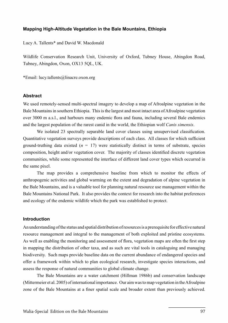
Mapping High-Altitude Vegetation in the Bale Mountains, Ethiopia

Lucy A. Tallents* and David W. Macdonald

Wildlife Conservation Research Unit, University of Oxford, Tubney House, Abingdon Road, Tubney, Abingdon, Oxon, Ox13 5qL, UK.

*Email: [email protected]

Abstract

We used remotely-sensed multi-spectral imagery to develop a map of Afroalpine vegetation in the Bale Mountains in southern Ethiopia. This is the largest and most intact area of Afroalpine vegetation over 3000 m a.s.l., and harbours many endemic flora and fauna, including several Bale endemics and the largest population of the rarest canid in the world, the Ethiopian wolf Canis simensis.

We isolated 23 spectrally separable land cover classes using unsupervised classification. Quantitative vegetation surveys provide descriptions of each class. All classes for which sufficient ground-truthing data existed (n = 17) were statistically distinct in terms of substrate, species composition, height and/or vegetation cover. The majority of classes identified discrete vegetation communities, while some represented the interface of different land cover types which occurred in the same pixel.

The map provides a comprehensive baseline from which to monitor the effects of anthropogenic activities and global warming on the extent and degradation of alpine vegetation in the Bale Mountains, and is a valuable tool for planning natural resource use management within the Bale Mountains National Park. It also provides the context for research into the habitat preferences and ecology of the endemic wildlife which the park was established to protect.

Introduction

An understanding of the status and spatial distribution of resources is a prerequisite for effective natural resource management and integral to the management of both exploited and pristine ecosystems. As well as enabling the monitoring and assessment of flora, vegetation maps are often the first step in mapping the distribution of other taxa, and as such are vital tools in cataloguing and managing biodiversity. Such maps provide baseline data on the current abundance of endangered species and offer a framework within which to plan ecological research, investigate species interactions, and assess the response of natural communities to global climate change.

The Bale Mountains are a water catchment (Hillman 1986b) and conservation landscape (Mittermeier et al. 2005) of international importance. Our aim was to map vegetation in the Afroalpine zone of the Bale Mountains at a finer spatial scale and broader extent than previously achieved.


Such a map is necessary to investigate fine-scale patterns of habitat selection and dependency of the endangered and endemic alpine species. It provides a baseline from which to monitor the effect of anthropogenic activities on the alpine plant communities and informs decision-making by the national park authorities about how to minimise potentially adverse impacts on ecosystem services provided by the park.

The Bale Mountains are in the southern highlands of Ethiopia (06°41’N, 39°03’E and 07°18’N, 40°00’E), and represent the largest area in Africa of Afroalpine vegetation over 3000m (Yalden, 1983). The contiguous massif is 2067 km2, or 17.5% of African land above 3000m, and is the most intact remnant of original highland vegetation (Brooks et al. 2004). The massif comprises one of Conservation International’s Key Biodiversity Areas, included in their Eastern Afromontane hotspot (Brooks et al. 2004), and is listed as an Important Bird Area (IBA) by Birdlife International (Fishpool and Evans 2001). Many of the species endemic to Ethiopia are associated with the high-altitude moorland and grassland abundant in Bale (Yalden 1983). These national endemics include 19 species of mammal, three of which are found only in the Bale mountains (Asefa this edition): the giant molerat Tachyoryctes macrocephalus, unstriped grass rat Arvicanthis blicki and harsh-furred mouse Lophuromys melanonyx (Yalden and Largen 1992). The area is also a hotspot of endemicity for amphibians (Largen and Spawls this edition) and birds (Shimelis et al this edition), and supports a diverse raptor guild which exploits the abundant rodent fauna (Birdlife International 2005). The flora of the alpine zone is equally notable, with no less than 163 highland endemics, 27 of which are restricted to Bale itself, including Alchemilla haumannii (Birdlife International 2006) and Euryops prostratus (Williams et al. 2004).

The BMNP was created in 1969 with the purpose of protecting the endemic mountain nyala Tragelaphus buxtoni and Ethiopian wolf Canis simensis, and the alpine zone and the tropical forest on the southern slopes (Hillman 1986a). The park boundaries encompass 52% of the land above 3000 m a.s.l., with most of the remainder in Somkero-Korduro, a spur to the west, and in Gaysay to the north. The area is characterised by high-altitude plateaux and wide valleys bounded by volcanic plugs, lava flows and the precipitous Harenna escarpment to the south (Miehe and Miehe 1994).

The first map of vegetation within and around the BMNP was published by Waltermire (1975, cited in Hillman 1986a), and most work has focussed on the montane forest and ericaceous belt (e.g. Miehe and Miehe 1993, 1994; Bussmann 1997, Hillman 1986a). These brief descriptions of the vegetation are restricted to small areas at the top of altitudinal transects, and the initial maps were hand-drawn from field surveys and aerial photography on 1:50,000 base-maps (Ethiopian Mapping Agency). More detail is presented in the management plans of the BMNP (Hillman 1986a, Nelson this edition), which includes a map of five subdivisions of the park, based on altitude and dominant flora. This map was derived from ground-surveys, 1:50,000 base maps, Landsat imagery and EMA aerial photography from the late 1960s and early 1970s. Nine of the 16 vegetation types described fall within the alpine grassland and moorland (subalpine) zones. Although useful for broad-scale management, these few categories do not adequately represent the complexity of vegetation communities, or the diversity of the animal communities that inhabit them. Other published studies


of the alpine vegetation have been with reference to suitable habitat for the Ethiopian wolf (Marino 2003, Sillero-Zubiri et al. 1997) and maps have been limited in spatial resolution (Hillman 1986a) or extent (Marino 2003), both of which constrain their use for more general research or management. In conclusion, the park currently lacks a detailed map of land cover throughout the alpine zone, and this study aims to fill that gap.

Methods

To summarise our approach, we derived principal components of the Landsat spectral bands, and used them as the input for an unsupervised classification to isolate spectrally unique land cover classes. We created a qualitative description of each land cover class based on substantial ground-truthing data and expert knowledge of the area. We then tested whether land cover classes were distinguishable from each other in terms of their substrate, plant cover and height, and species composition, using quantitative vegetation survey data.

Preparation of the satellite imagery

Variations in microclimate, substrate and drainage create a fine-scale mosaic of Afroalpine vegetation, making it difficult to delineate large enough homogeneous patches as training sites for supervised classification. Inaccurate classifications can result, especially where mixed pixels represent a large extent of the image (Cingolani et al. 2004). Terrain complexity in mountainous regions can also impair supervised classification through the inclusion of pixels with varying slope/aspect and therefore illumination in the same training sample (Townshend and Justice 1980). For these reasons, we chose unsupervised classification (Mather 1987) to map land cover, and determined the plant species composition and substrate of each class post-hoc. This exploits the full range of reflectance values, ensuring that all combinations of spectral characteristics are represented, and that classes are clearly distinguishable from each other (Lillesand et al. 2004).

Erdas (v8.7, Leica Geosystems GIS & Mapping LLC) was used to manipulate and analyse remotely-sensed data. The Landsat 7 ETM+ image (NASA Landsat Program, 2005: path 167 row 055, 28th Nov 2000) was downloaded from the Global Land Cover Facility (www.landcover.org). These free geotiffs contain all nine Landsat spectral bands. They are projected in UTM using the WGS84 datum and reference ellipsoid, and orthorectified using nearest neighbour sampling (Tucker et al. 2004). The digital elevation model (DEM) from the Shuttle Radar Topographic Mission (SRTM)’s 3 arc second dataset (USGS 2006) was also downloaded from the GLCF in UTM WGS84.

Ground-control points were obtained using a Garmin 12 hand-held GPS (Garmin Ltd.) along readily-identifiable features such as rivers, lake edges, lava cliffs and roads. Alignment of the Landsat image and ground data was slightly improved by a sub-pixel shift of 10m south and 20 m west applied to the Landsat image. Co-registration of the DEM was also improved by a linear shift of 180 m north.


A preliminary unsupervised classification of land above 2900m discriminated two classes of high-altitude vegetation. Lower-altitude forest and agricultural land was assigned to a third class, which was then masked (e.g. Lauver and Whistler 1993). The reduction in spectral variability of the image enhanced our ability to distinguish between the land cover types of interest.

A principal components analysis (PCA) on the eight non-panchromatic bands reduced dimensionality of the dataset by partitioning the majority of the spectral variation into fewer bands. This allowed us to remove spectral anomalies such as haze and banding (Jensen 1996) which were separated into the last components and excluded from the classification.

Unsupervised classification

We set the minimum number of classes as the number of habitat types that could be distinguished visually in false-colour composites by an observer familiar with the area. We examined exploratory classifications using 20 to 50 classes to assess the representation of known land cover types and the ability of the classification to distinguish between them. We determined the appropriate number of classes by a combination of testing for statistical separation of classes, and expert knowledge of the site. It is important to include expert knowledge in the classification process, particularly in topographically complex areas (Shrestha and Zinck 2001), to ensure that the map represents the fine distinctions needed by end users, and isolates land cover types of particular research or management interest.

Clusters were initialised along the principal axis, using the automatic scaling range option. The convergence threshold was set to 0.98, with 30 as the maximum number of iterations, and every cell in the grid used as input for the clustering algorithm (Leica Geosystems 2003).

Our criterion for class separation was that ellipses plotted in full-dimensional feature space showed no overlap at 1.28 standard deviations (SD). This allowed for 20% of the pixels to lie in the extremes beyond the ellipse, potentially falling within the signature of another class, but incorporating 80% of the pixels in non-overlapping space. Separation of class means was assessed by Euclidean distance, and spectral relationships between classes were illustrated using a dendrogram, based on complete linkage agglomeration (Leica Geosystems 1991-2003).

Vegetation sampling

Clustered stratified random sampling was used to survey vegetation intensively within the areas of primary interest in the Afroalpine zone: the Web Valley and Sanetti Plateau. Grid cells of 200 x 200m were chosen at random, and five locations coordinates were generated random within each cell. See Tallents (2007) for further detail on the sampling design. Data from 442 vegetation sampling locations and the central four points of 112 rodent trapping grids were included; 39 of the latter were located outside the two sites of primary interest. Extensive surveys throughout other areas of the Bale Mountains resulted in qualitative descriptions of the vegetation at a further 132 random locations, ensuring that all land cover classes were represented in the ground-truthing data.


Observers located each point by GPS, and four subsamples (N/E/S/W) were taken at each location. Sampling density was equivalent to that on rodent trapping grids, with 5m between subsamples. For each plant species intersected by the sampling rod, observers recorded the maximum height, plant part (leaf, stem or flower) and colour (to indicate seasonal changes in nutritional quality). Substrate (earth, rock or water), date, time and observer were also recorded.

Vegetation was surveyed by observers without formal botanical expertise, limiting the number of taxa which could be identified to species level. Surveys occurred in both wet and dry seasons, so the flower structures necessary for identification of grasses and some herbaceous species were not always present. All grass-like plants were therefore split into two categories only: wetland sedges and grasses. Similarly, no attempt was made to distinguish between different mosses or lichens.

Ground-truthing and statistical analysisThe land cover type represented by each class was determined using qualitative habitat descriptions, supplemented by visual examination of aerial photographs, false-colour composites, 199 ground-truthing photographs and familiarity with areas gained during field surveys between April 2003 and April 2005. To assess how related clusters of classes in the distance dendrogram differed from one another, pairwise statistical comparisons were made at each node for which sufficient data existed. Differences in plant species composition and substrate were assessed using contingency tables. General Linear Models (GLMs) were used to test for differences in altitude, slope, aspect, and percent vegetation cover, and mean sward height was also compared after accounting for species composition and altitude. Tests used all classes and all species for which enough data were available; sample sizes varied depending upon which classes were being compared.

The combination of mountainous terrain, low sun elevation (52.1 degrees) and sun azimuth (139.6 degrees) at the time of satellite image capture caused large differences in illumination between southeast and northwest slopes. This meant that classes on steeply sloping ground may have differed from each other only in the degree of illumination, rather than in species composition or density of vegetation. Therefore we calculated the incidence angle of the sun’s rays to describe the relative illumination of each pixel, and test for differences in average illumination between classes. The following formula was taken from Dozier and Frew (1990):

θi = arccos(cosθ0*cosS + sinθ0*sinS*cos(Φ0 − A))

where θi = illumination angle, θ0= solar elevation, S = pixel slope, Φ0 = solar azimuth and A = pixel aspect.

We investigated seasonal changes in photosynthetic activity by categorising plants into ‘alive’ (flowering or green) or ‘dead/dormant’ (brown or yellow). This was hard to determine for some pubescent species such as Helichrysum sp.; the status of these species was assigned as ‘unknown’ unless there was evidence of flowering.


We derived class descriptions from the quantitative surveys of substrate, cover, vegetation height and plant species composition, supplemented by photos, qualitative descriptions of vegetation structure, and familiarity with easily identifiable plant communities.

Results

Landsat PCA

Principal components (PCs) one to three captured over 95% of the variation in the Landsat pixel values, Table 1; see Tallents (2007) for factor loadings. PC1 isolated the factors which most strongly influenced reflectance in all wavelengths, contrasting water bodies and densely vegetated land with highly reflective bare soil. It was positively correlated with illumination (r = 0.44), separating heavily shaded from sun-facing slopes. PC2 had high values in cool, damp areas with high plant productivity such as drainage lines, and was lower in the arid Tullu Deemtu rain shadow and well-drained lava slopes. PC3 correlated strongly with altitude (r = -0.65), contrasting the Helichrysum-dominated high plateaux with the lower-altitude grassy valleys.

Table 1. Eigenvalues and variability captured by the Landsat image principal components.PC Eigenvalue Cumulative %1 4.99 62.392 1.47 80.793 1.14 95.064 0.27 98.395 0.06 99.166 0.04 99.657 0.02 99.958 < 0.01 100.00

PC8 only described differences between the two highly correlated thermal bands, and appeared as spatially random speckle, with some striping characteristic of the scanning path. PC7 isolated speckle probably associated with the resampling undertaken during orthoregistration, and was discarded along with PC8. The remaining six PCS captured over 99% of the variability in the data (Table 1), and formed the input for the classification. PCs 4 to 6 were retained despite their relatively low information content because they highlighted features of interest and it was expected that they would allow discrimination between broadly similar land cover classes. The fact that components have low eigenvalues can simply indicate that the variability they encapsulate is very localized (Eastman and Fulk 1993), so they can help to distinguish rare habitat types or those which are spectrally similar despite being floristically distinct (Townshend and Justice 1980).

Classification

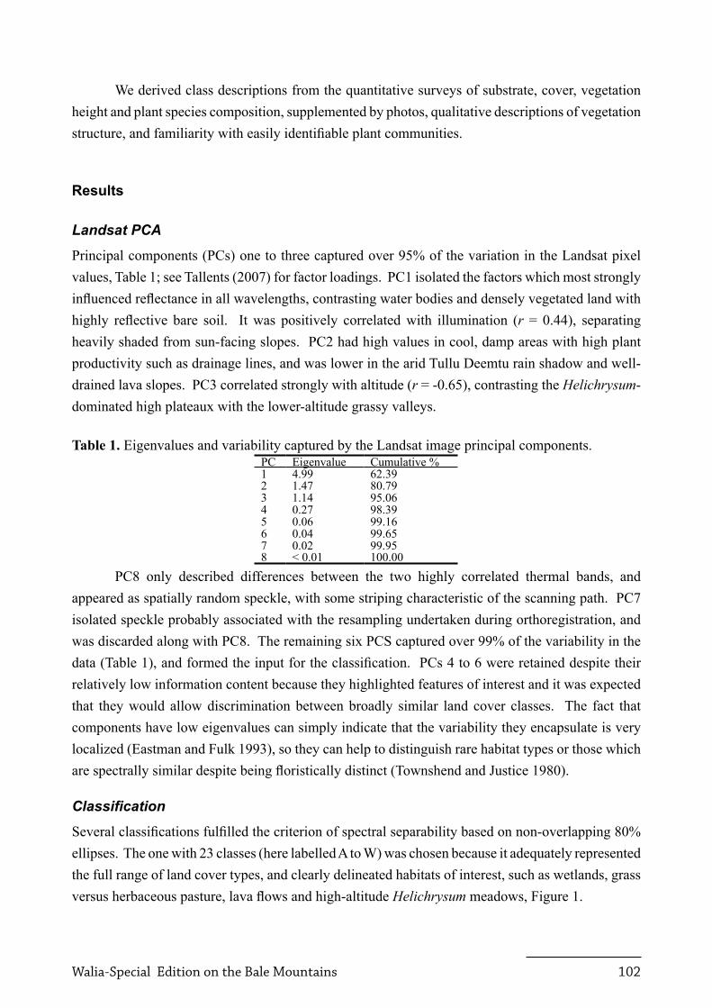
Several classifications fulfilled the criterion of spectral separability based on non-overlapping 80% ellipses. The one with 23 classes (here labelled A to W) was chosen because it adequately represented the full range of land cover types, and clearly delineated habitats of interest, such as wetlands, grass versus herbaceous pasture, lava flows and high-altitude Helichrysum meadows, Figure 1.

Wal

ia-S

peci

al E

diti

on o

n th

e Ba

le M

ount

ains

103

Figu

re 1

. Afr

oalp

ine

vege

tatio

n in

the

Bal

e M

ount

ains

. See

lege

nd fo

r pla

nt sp

ecie

s abb

revi

atio

ns.


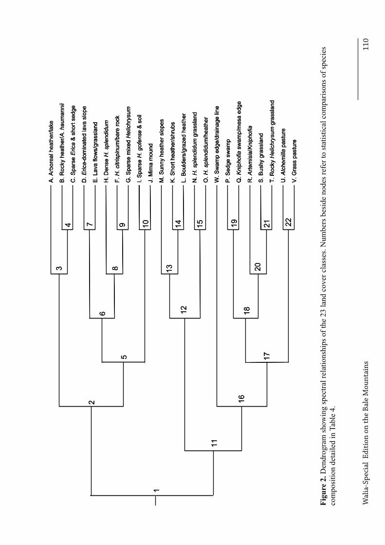
Where sufficient ground-truthing samples were available, class clustering in the distance dendrogram could be explained by the dominance of particular species, the degree of soil waterlogging, the coverage of rock/open water/vegetation, vegetation height, or topography (altitude/slope/illumination, Table 2).

Table 2. Topographic characteristics and survey sample sizes of land cover classes. See Table 3 for class names.

Class Median altitude(m)

Mean slope(°)

Mean illuminationCos(θi)

Pointsamples

A 3779 16.0 0.43 6B 3711 11.3 0.56 24C 3654 12.7 0.57 51D 3793 10.8 0.54 11E 3780 8.2 0.62 39F 3973 7.6 0.57 307G 4088 6.6 0.61 197H 4089 5.3 0.62 238I 4079 5.0 0.63 432J 4102 3.5 0.61 343K 3506 14.5 0.68 22L 3743 11.2 0.67 21M 3560 18.2 0.76 4N 3890 5.6 0.66 99O 3808 11.6 0.70 14P 3730 7.1 0.61 122q 3530 8.3 0.59 140R 3577 9.5 0.67 99S 3694 5.9 0.62 263T 3698 6.0 0.64 271U 3490 5.9 0.63 831V 3539 4.3 0.62 1148W 3444 12.7 0.68 70Total 4752

Vegetation surveys

We recorded 16,672 plants in 45 taxa, of which 82% were identified to species level and a further 7% to genus level. Unidentified plants comprised only 1.1% of the dataset, and the remainder were assigned to the broad classes of grasses, mosses and lichens.Seasonal differences were observed in the degree of open water (contingency table: Χ2 = 35.6, p < 0.001, n = 4104), with more in the wet season (3.2% cover versus 0.7% in the dry season). No differences were found in the percent cover of earth or rock substrate between seasons. A greater proportion of the vegetation was recorded as alive or actively growing in the wet season (76.9% versus 43.4% in the dry season, Χ1 = 395.5, p < 0.001, n = 3614).

Differences between land cover classes

Most land cover classes could also be distinguished from their nearest neighbour using the quantitative survey data. Exceptions were classes A, B and C from each other, classes K, L and M from each


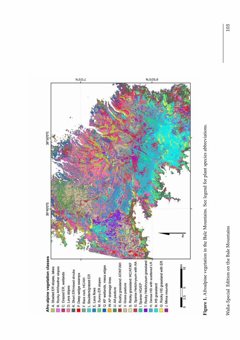
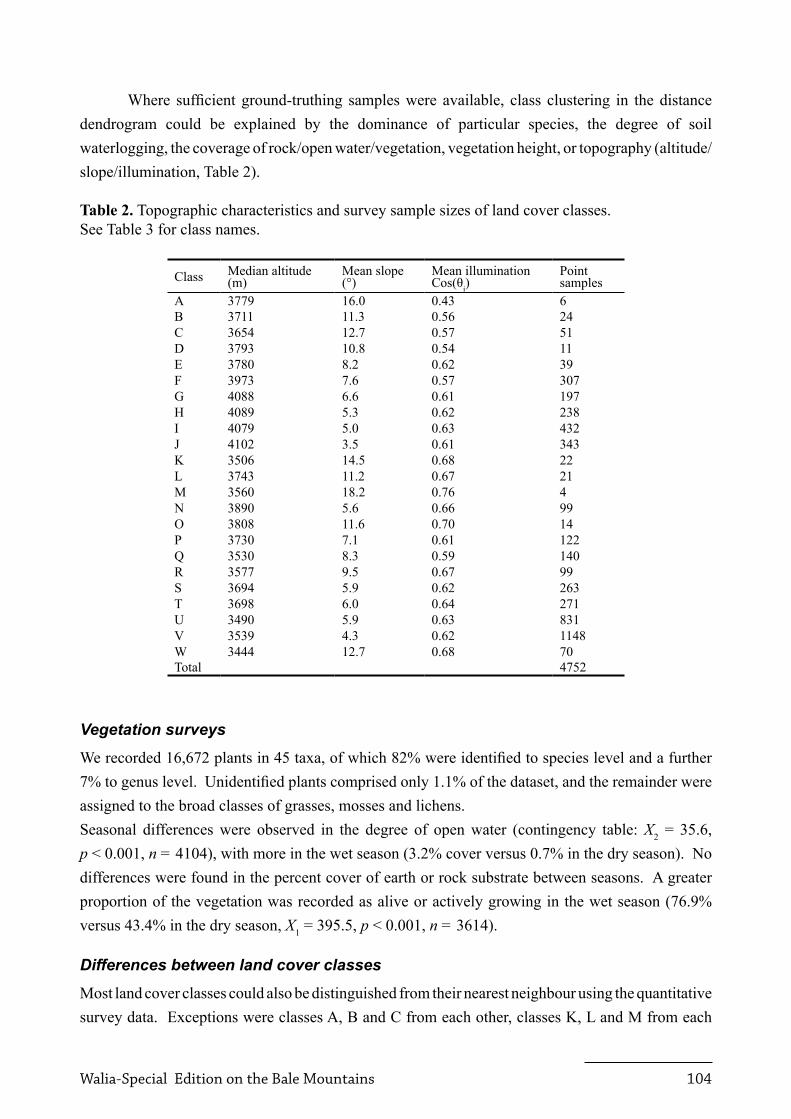
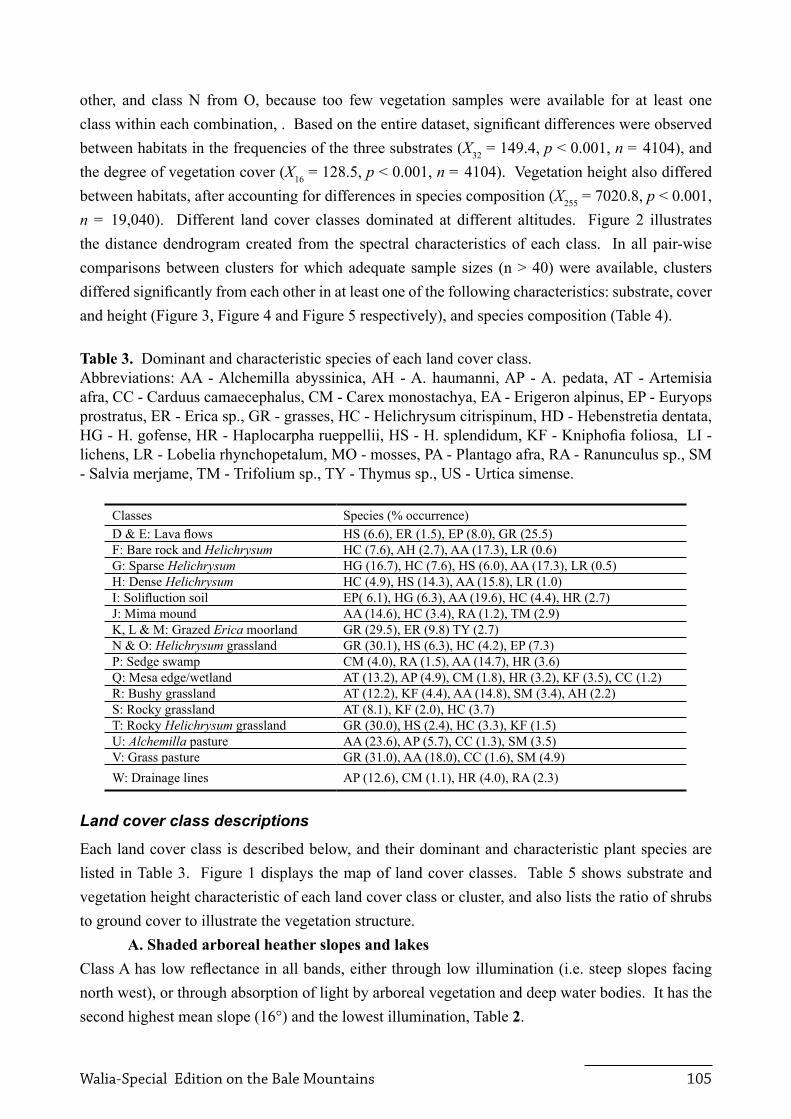
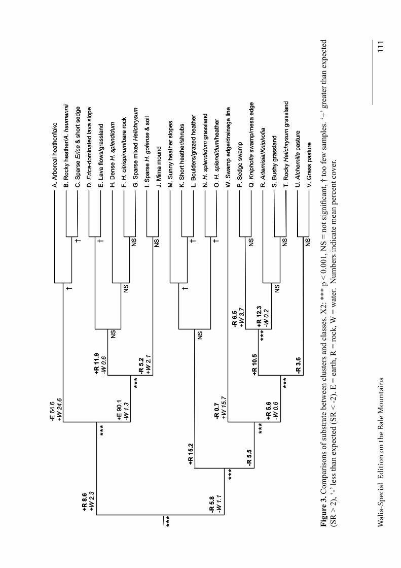
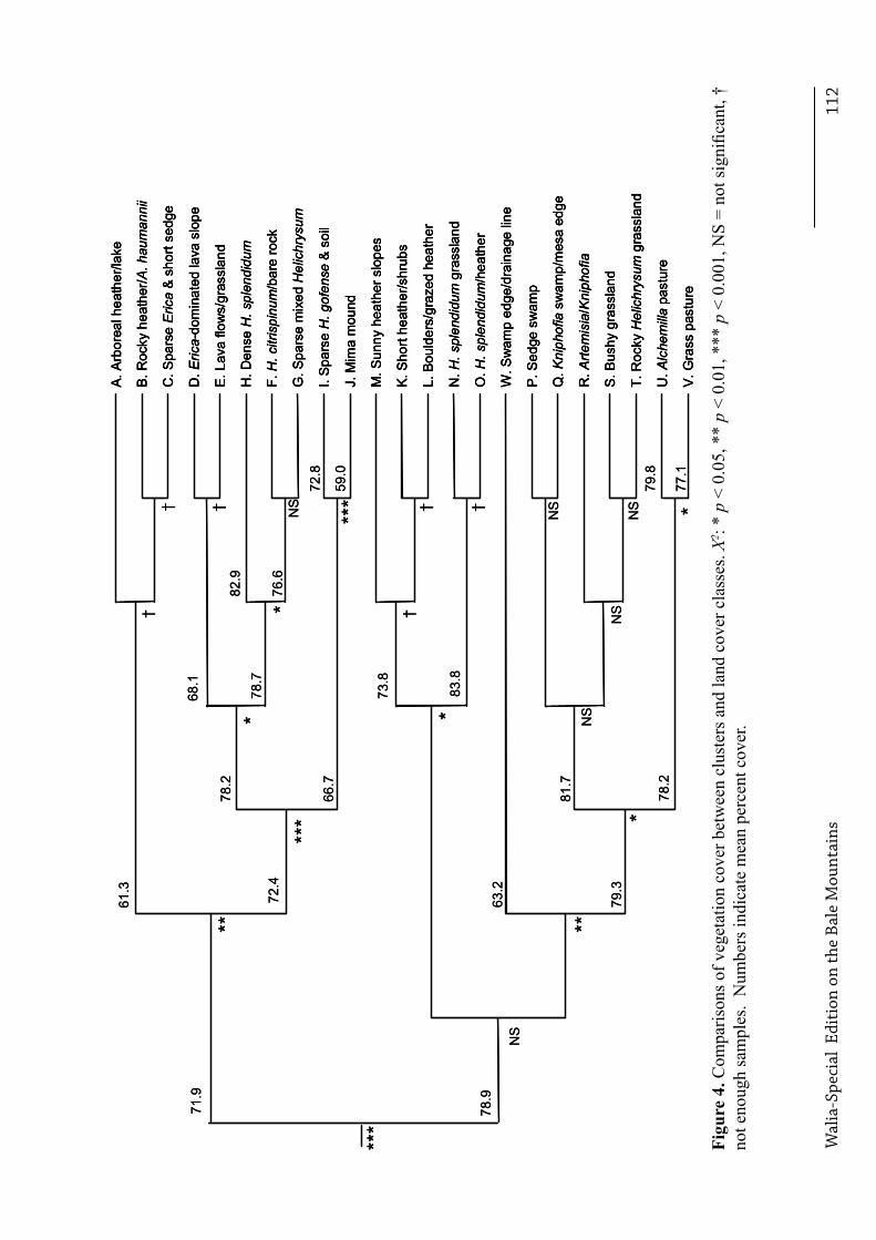
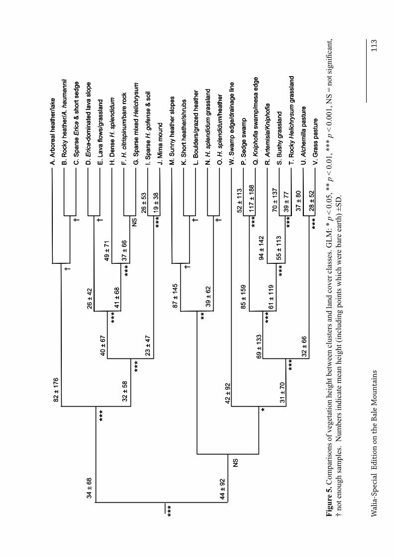
other, and class N from O, because too few vegetation samples were available for at least one class within each combination, . Based on the entire dataset, significant differences were observed between habitats in the frequencies of the three substrates (Χ32 = 149.4, p < 0.001, n = 4104), and the degree of vegetation cover (Χ16 = 128.5, p < 0.001, n = 4104). Vegetation height also differed between habitats, after accounting for differences in species composition (Χ255 = 7020.8, p < 0.001, n = 19,040). Different land cover classes dominated at different altitudes. Figure 2 illustrates the distance dendrogram created from the spectral characteristics of each class. In all pair-wise comparisons between clusters for which adequate sample sizes (n > 40) were available, clusters differed significantly from each other in at least one of the following characteristics: substrate, cover and height (Figure 3, Figure 4 and Figure 5 respectively), and species composition (Table 4).

Table 3. Dominant and characteristic species of each land cover class. Abbreviations: AA - Alchemilla abyssinica, AH - A. haumanni, AP - A. pedata, AT - Artemisia afra, CC - Carduus camaecephalus, CM - Carex monostachya, EA - Erigeron alpinus, EP - Euryops prostratus, ER - Erica sp., GR - grasses, HC - Helichrysum citrispinum, HD - Hebenstretia dentata, HG - H. gofense, HR - Haplocarpha rueppellii, HS - H. splendidum, KF - Kniphofia foliosa, LI - lichens, LR - Lobelia rhynchopetalum, MO - mosses, PA - Plantago afra, RA - Ranunculus sp., SM - Salvia merjame, TM - Trifolium sp., TY - Thymus sp., US - Urtica simense.

Classes Species (% occurrence)D & E: Lava flows HS (6.6), ER (1.5), EP (8.0), GR (25.5)F: Bare rock and Helichrysum HC (7.6), AH (2.7), AA (17.3), LR (0.6)G: Sparse Helichrysum HG (16.7), HC (7.6), HS (6.0), AA (17.3), LR (0.5)H: Dense Helichrysum HC (4.9), HS (14.3), AA (15.8), LR (1.0)I: Solifluction soil EP( 6.1), HG (6.3), AA (19.6), HC (4.4), HR (2.7)J: Mima mound AA (14.6), HC (3.4), RA (1.2), TM (2.9)K, L & M: Grazed Erica moorland GR (29.5), ER (9.8) TY (2.7)N & O: Helichrysum grassland GR (30.1), HS (6.3), HC (4.2), EP (7.3)P: Sedge swamp CM (4.0), RA (1.5), AA (14.7), HR (3.6)q: Mesa edge/wetland AT (13.2), AP (4.9), CM (1.8), HR (3.2), KF (3.5), CC (1.2)R: Bushy grassland AT (12.2), KF (4.4), AA (14.8), SM (3.4), AH (2.2)S: Rocky grassland AT (8.1), KF (2.0), HC (3.7)T: Rocky Helichrysum grassland GR (30.0), HS (2.4), HC (3.3), KF (1.5)U: Alchemilla pasture AA (23.6), AP (5.7), CC (1.3), SM (3.5)V: Grass pasture GR (31.0), AA (18.0), CC (1.6), SM (4.9)W: Drainage lines AP (12.6), CM (1.1), HR (4.0), RA (2.3)

Land cover class descriptions

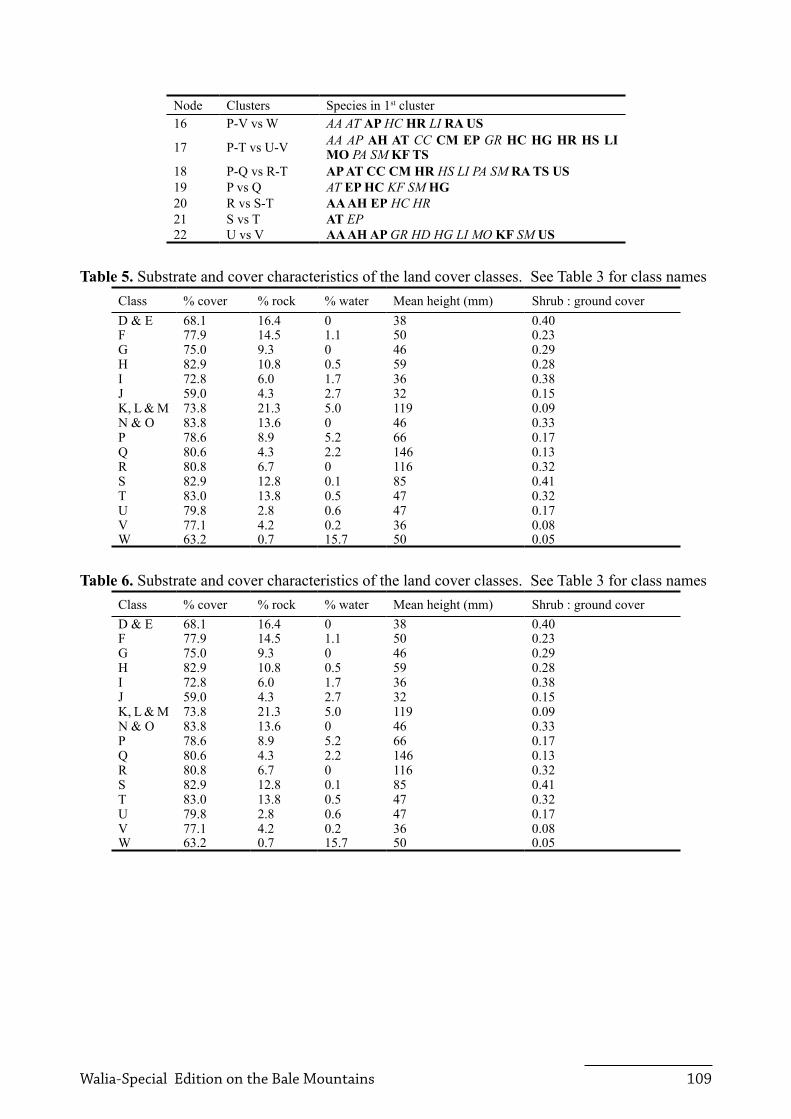
Each land cover class is described below, and their dominant and characteristic plant species are listed in Table 3. Figure 1 displays the map of land cover classes. Table 5 shows substrate and vegetation height characteristic of each land cover class or cluster, and also lists the ratio of shrubs to ground cover to illustrate the vegetation structure.

A. Shaded arboreal heather slopes and lakesClass A has low reflectance in all bands, either through low illumination (i.e. steep slopes facing north west), or through absorption of light by arboreal vegetation and deep water bodies. It has the second highest mean slope (16°) and the lowest illumination, Table 2.


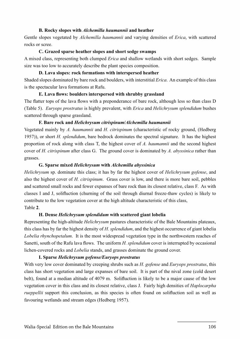
B. Rocky slopes with Alchemilla haumannii and heatherGentle slopes vegetated by Alchemilla haumannii and varying densities of Erica, with scattered rocks or scree.

C. Grazed sparse heather slopes and short sedge swampsA mixed class, representing both clumped Erica and shallow wetlands with short sedges. Sample size was too low to accurately describe the plant species composition.

D. Lava slopes: rock formations with interspersed heatherShaded slopes dominated by bare rock and boulders, with interstitial Erica. An example of this class is the spectacular lava formations at Rafu.

E. Lava flows: boulders interspersed with shrubby grasslandThe flatter tops of the lava flows with a preponderance of bare rock, although less so than class D (Table 5). Euryops prostratus is highly prevalent, with Erica and Helichrysum splendidum bushes scattered through sparse grassland.

F. Bare rock and Helichrysum citrispinum/Alchemilla haumanniiVegetated mainly by A. haumannii and H. citrispinum (characteristic of rocky ground, (Hedberg 1957)), or short H. splendidum, bare bedrock dominates the spectral signature. It has the highest proportion of rock along with class T, the highest cover of A. haumannii and the second highest cover of H. citrispinum after class G. The ground cover is dominated by A. abyssinica rather than grasses.

G. Sparse mixed Helichrysum with Alchemilla abyssinicaHelichrysum sp. dominate this class; it has by far the highest cover of Helichrysum gofense, and also the highest cover of H. citrispinum. Grass cover is low, and there is more bare soil, pebbles and scattered small rocks and fewer expanses of bare rock than its closest relative, class F. As with classes I and J, solifluction (churning of the soil through diurnal freeze-thaw cycles) is likely to contribute to the low vegetation cover at the high altitude characteristic of this class, Table 2.

h. Dense Helichrysum splendidum with scattered giant lobeliaRepresenting the high-altitude Helichrysum pastures characteristic of the Bale Mountains plateaux, this class has by far the highest density of H. splendidum, and the highest occurrence of giant lobelia Lobelia rhynchopetalum. It is the most widespread vegetation type in the northwestern reaches of Sanetti, south of the Rafu lava flows. The uniform H. splendidum cover is interrupted by occasional lichen-covered rocks and Lobelia stands, and grasses dominate the ground cover.

I. Sparse Helichrysum gofense/Euryops prostratusWith very low cover dominated by creeping shrubs such as H. gofense and Euryops prostratus, this class has short vegetation and large expanses of bare soil. It is part of the nival zone (cold desert belt), found at a median altitude of 4079 m. Solifluction is likely to be a major cause of the low vegetation cover in this class and its closest relative, class J. Fairly high densities of Haplocarpha rueppellii support this conclusion, as this species is often found on solifluction soil as well as favouring wetlands and stream edges (Hedberg 1957).


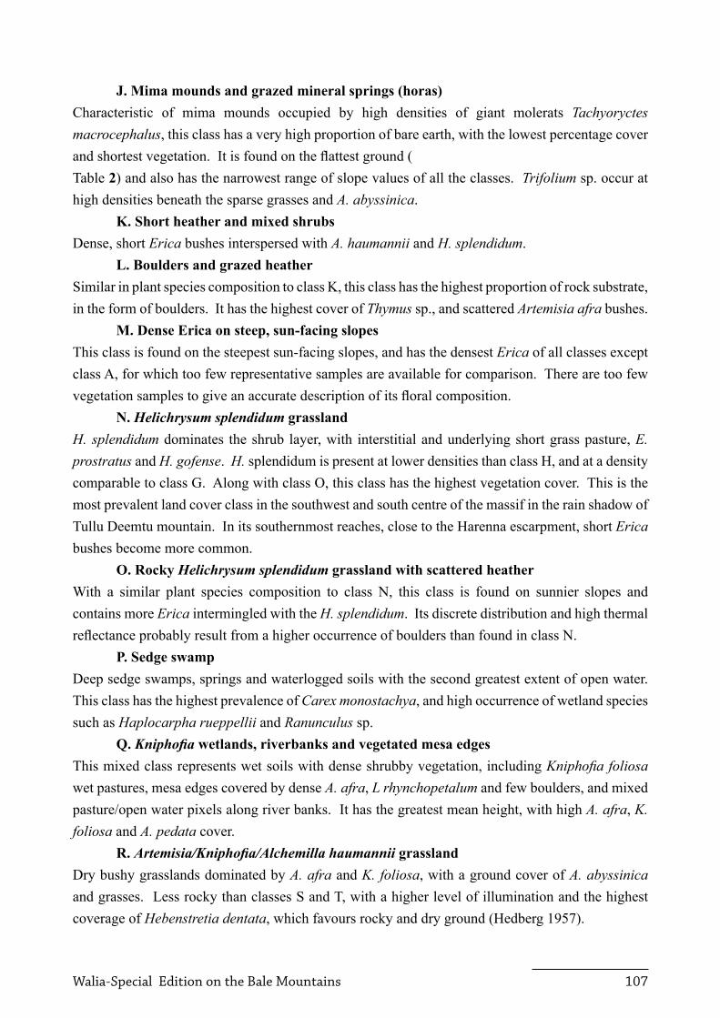
J. mima mounds and grazed mineral springs (horas)Characteristic of mima mounds occupied by high densities of giant molerats Tachyoryctes macrocephalus, this class has a very high proportion of bare earth, with the lowest percentage cover and shortest vegetation. It is found on the flattest ground (Table 2) and also has the narrowest range of slope values of all the classes. Trifolium sp. occur at high densities beneath the sparse grasses and A. abyssinica.

K. Short heather and mixed shrubsDense, short Erica bushes interspersed with A. haumannii and H. splendidum.

L. Boulders and grazed heatherSimilar in plant species composition to class K, this class has the highest proportion of rock substrate, in the form of boulders. It has the highest cover of Thymus sp., and scattered Artemisia afra bushes.

M. Dense Erica on steep, sun-facing slopesThis class is found on the steepest sun-facing slopes, and has the densest Erica of all classes except class A, for which too few representative samples are available for comparison. There are too few vegetation samples to give an accurate description of its floral composition.

N. Helichrysum splendidum grasslandH. splendidum dominates the shrub layer, with interstitial and underlying short grass pasture, E. prostratus and H. gofense. H. splendidum is present at lower densities than class H, and at a density comparable to class G. Along with class O, this class has the highest vegetation cover. This is the most prevalent land cover class in the southwest and south centre of the massif in the rain shadow of Tullu Deemtu mountain. In its southernmost reaches, close to the Harenna escarpment, short Erica bushes become more common.

O. Rocky Helichrysum splendidum grassland with scattered heatherWith a similar plant species composition to class N, this class is found on sunnier slopes and contains more Erica intermingled with the H. splendidum. Its discrete distribution and high thermal reflectance probably result from a higher occurrence of boulders than found in class N.

P. Sedge swampDeep sedge swamps, springs and waterlogged soils with the second greatest extent of open water. This class has the highest prevalence of Carex monostachya, and high occurrence of wetland species such as Haplocarpha rueppellii and Ranunculus sp.

Q. Kniphofia wetlands, riverbanks and vegetated mesa edgesThis mixed class represents wet soils with dense shrubby vegetation, including Kniphofia foliosa wet pastures, mesa edges covered by dense A. afra, L rhynchopetalum and few boulders, and mixed pasture/open water pixels along river banks. It has the greatest mean height, with high A. afra, K. foliosa and A. pedata cover.

r. Artemisia/Kniphofia/Alchemilla haumannii grasslandDry bushy grasslands dominated by A. afra and K. foliosa, with a ground cover of A. abyssinica and grasses. Less rocky than classes S and T, with a higher level of illumination and the highest coverage of Hebenstretia dentata, which favours rocky and dry ground (Hedberg 1957).


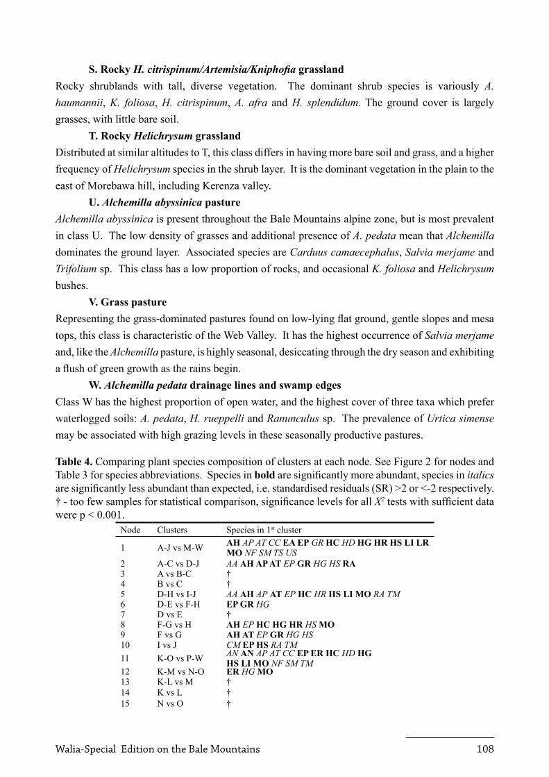
S. Rocky H. citrispinum/Artemisia/Kniphofia grasslandRocky shrublands with tall, diverse vegetation. The dominant shrub species is variously A. haumannii, K. foliosa, H. citrispinum, A. afra and H. splendidum. The ground cover is largely grasses, with little bare soil.

T. Rocky Helichrysum grasslandDistributed at similar altitudes to T, this class differs in having more bare soil and grass, and a higher frequency of Helichrysum species in the shrub layer. It is the dominant vegetation in the plain to the east of Morebawa hill, including Kerenza valley.

u. Alchemilla abyssinica pastureAlchemilla abyssinica is present throughout the Bale Mountains alpine zone, but is most prevalent in class U. The low density of grasses and additional presence of A. pedata mean that Alchemilla dominates the ground layer. Associated species are Carduus camaecephalus, Salvia merjame and Trifolium sp. This class has a low proportion of rocks, and occasional K. foliosa and Helichrysum bushes.

V. Grass pastureRepresenting the grass-dominated pastures found on low-lying flat ground, gentle slopes and mesa tops, this class is characteristic of the Web Valley. It has the highest occurrence of Salvia merjame and, like the Alchemilla pasture, is highly seasonal, desiccating through the dry season and exhibiting a flush of green growth as the rains begin.

W. Alchemilla pedata drainage lines and swamp edgesClass W has the highest proportion of open water, and the highest cover of three taxa which prefer waterlogged soils: A. pedata, H. rueppelli and Ranunculus sp. The prevalence of Urtica simense may be associated with high grazing levels in these seasonally productive pastures.

Table 4. Comparing plant species composition of clusters at each node. See Figure 2 for nodes and Table 3 for species abbreviations. Species in bold are significantly more abundant, species in italics are significantly less abundant than expected, i.e. standardised residuals (SR) >2 or <-2 respectively. † - too few samples for statistical comparison, significance levels for all Χ2 tests with sufficient data were p < 0.001.

Node Clusters Species in 1st cluster

1 A-J vs M-W Ah AP AT CC EA EP GR hC HD hG hr hS LI Lr mO NF SM TS US

2 A-C vs D-J AA Ah AP AT EP Gr HG HS rA3 A vs B-C †4 B vs C †5 D-H vs I-J AA Ah AP AT EP hC HR hS LI mO RA TM6 D-E vs F-H EP Gr HG7 D vs E †8 F-G vs H Ah EP hC hG hr HS mO9 F vs G Ah AT EP Gr HG HS10 I vs J CM EP hS RA TM11 K-O vs P-W AN AN AP AT CC EP Er hC HD hG

hS LI mO NF SM TM12 K-M vs N-O Er HG mO13 K-L vs M †14 K vs L †15 N vs O †


Node Clusters Species in 1st cluster16 P-V vs W AA AT AP HC hr LI rA uS

17 P-T vs U-V AA AP Ah AT CC Cm EP GR hC hG hr hS LI mO PA SM KF TS

18 P-q vs R-T AP AT CC Cm hr HS LI PA SM rA TS uS19 P vs q AT EP hC KF SM hG20 R vs S-T AA Ah EP HC HR21 S vs T AT EP22 U vs V AA Ah AP GR HD HG LI MO KF SM uS

Table 5. Substrate and cover characteristics of the land cover classes. See Table 3 for class namesClass % cover % rock % water Mean height (mm) Shrub : ground coverD & E 68.1 16.4 0 38 0.40F 77.9 14.5 1.1 50 0.23G 75.0 9.3 0 46 0.29H 82.9 10.8 0.5 59 0.28I 72.8 6.0 1.7 36 0.38J 59.0 4.3 2.7 32 0.15K, L & M 73.8 21.3 5.0 119 0.09N & O 83.8 13.6 0 46 0.33P 78.6 8.9 5.2 66 0.17q 80.6 4.3 2.2 146 0.13R 80.8 6.7 0 116 0.32S 82.9 12.8 0.1 85 0.41T 83.0 13.8 0.5 47 0.32U 79.8 2.8 0.6 47 0.17V 77.1 4.2 0.2 36 0.08W 63.2 0.7 15.7 50 0.05

Table 6. Substrate and cover characteristics of the land cover classes. See Table 3 for class namesClass % cover % rock % water Mean height (mm) Shrub : ground coverD & E 68.1 16.4 0 38 0.40F 77.9 14.5 1.1 50 0.23G 75.0 9.3 0 46 0.29H 82.9 10.8 0.5 59 0.28I 72.8 6.0 1.7 36 0.38J 59.0 4.3 2.7 32 0.15K, L & M 73.8 21.3 5.0 119 0.09N & O 83.8 13.6 0 46 0.33P 78.6 8.9 5.2 66 0.17q 80.6 4.3 2.2 146 0.13R 80.8 6.7 0 116 0.32S 82.9 12.8 0.1 85 0.41T 83.0 13.8 0.5 47 0.32U 79.8 2.8 0.6 47 0.17V 77.1 4.2 0.2 36 0.08W 63.2 0.7 15.7 50 0.05

Wal

ia-S

peci

al E

diti

on o

n th

e Ba

le M

ount

ains

110

A. A

rbor

eal h

eath

er/la

ke

B. R

ocky

hea

ther

/A. h

aum

anni

i

C. S

pars

e E

rica

& s

hort

sedg

e

D. E

rica-

dom

inat

ed la

va s

lope

E. L

ava

flow

s/gr

assl

and

H. D

ense

H. s

plen

didu

m

F. H

. citr

ispi

num

/bar

e ro

ck

G. S

pars

e m

ixed

Hel

ichr

ysum

I. S

pars

e H

. gof

ense

& s

oil

J. M

ima

mou

nd

M. S

unny

hea

ther

slo

pes

K. S

hort

heat

her/s

hrub

s

L. B

ould

ers/

graz

ed h

eath

er

N. H

. spl

endi

dum

gra

ssla

nd

O.H

. spl

endi

dum

/hea

ther

W. S

wam

p ed

ge/d

rain

age

line

P. S

edge

sw

amp

Q. K

niph

ofia

swam

p/m

esa

edge

R. A

rtem

isia

/Kni

phof

ia

S. B

ushy

gra

ssla

nd

T. R

ocky

Hel

ichr

ysum

gras

slan

d

U. A

lche

mill

apa

stur

e

V. G

rass

pas

ture

2

11

16

12

76

83 13 2017

18

22211915141094

5

1

A. A

rbor

eal h

eath

er/la

ke

B. R

ocky

hea

ther

/A. h

aum

anni

i

C. S

pars

e E

rica

& s

hort

sedg

e

D. E

rica-

dom

inat

ed la

va s

lope

E. L

ava

flow

s/gr

assl

and

H. D

ense

H. s

plen

didu

m

F. H

. citr

ispi

num

/bar

e ro

ck

G. S

pars

e m

ixed

Hel

ichr

ysum

I. S

pars

e H

. gof

ense

& s

oil

J. M

ima

mou

nd

M. S

unny

hea

ther

slo

pes

K. S

hort

heat

her/s

hrub

s

L. B

ould

ers/

graz

ed h

eath

er

N. H

. spl

endi

dum

gra

ssla

nd

O.H

. spl

endi

dum

/hea

ther

W. S

wam

p ed

ge/d

rain

age

line

P. S

edge

sw

amp

Q. K

niph

ofia

swam

p/m

esa

edge

R. A

rtem

isia

/Kni

phof

ia

S. B

ushy

gra

ssla

nd

T. R

ocky

Hel

ichr

ysum

gras

slan

d

U. A

lche

mill

apa

stur

e

V. G

rass

pas

ture

A. A

rbor

eal h

eath

er/la

ke

B. R

ocky

hea

ther

/A. h

aum

anni

i

C. S

pars

e E

rica

& s

hort

sedg

e

D. E

rica-

dom

inat

ed la

va s

lope

E. L

ava

flow

s/gr

assl

and

H. D

ense

H. s

plen

didu

m

F. H

. citr

ispi

num

/bar

e ro

ck

G. S

pars

e m

ixed

Hel

ichr

ysum

I. S

pars

e H

. gof

ense

& s

oil

J. M

ima

mou

nd

M. S

unny

hea

ther

slo

pes

K. S

hort

heat

her/s

hrub

s

L. B

ould

ers/

graz

ed h

eath

er

N. H

. spl

endi

dum

gra

ssla

nd

O.H

. spl

endi

dum

/hea

ther

W. S

wam

p ed

ge/d

rain

age

line

P. S

edge

sw

amp

Q. K

niph

ofia

swam

p/m

esa

edge

R. A

rtem

isia

/Kni

phof

ia

S. B

ushy

gra

ssla

nd

T. R

ocky

Hel

ichr

ysum

gras

slan

d

U. A

lche

mill

apa

stur

e

V. G

rass

pas

ture

2

11

16

12

76

83 13 2017

18

22211915141094

5

1

Figu

re 2

. Den

drog

ram

show

ing

spec

tral r

elat

ions

hips

of t

he 2

3 la

nd c

over

cla

sses

. Num

bers

bes

ide

node

s ref

er to

stat

istic

al c

ompa

rison

s of s

peci

es

com

posi

tion

deta

iled

in T

able

4.

Wal

ia-S

peci

al E

diti

on o

n th

e Ba

le M

ount

ains

111

A. A

rbor

eal h

eath

er/la

ke

B. R

ocky

hea

ther

/A. h

aum

anni

i

C. S

pars

e E

rica

& s

hort

sedg

e

D. E

rica-

dom

inat

ed la

va s

lope

E. L

ava

flow

s/gr

assl

and

H. D

ense

H. s

plen

didu

m

F. H

. citr

ispi

num

/bar

e ro

ck

G. S

pars

e m

ixed

Hel

ichr

ysum

I. S

pars

e H

. gof

ense

& s

oil

J. M

ima

mou

nd

M. S

unny

hea

ther

slo

pes

K. S

hort

heat

her/s

hrub

s

L. B

ould

ers/

graz

ed h

eath

er

N. H

. spl

endi

dum

gra

ssla

nd

O.H

. spl

endi

dum

/hea

ther

W. S

wam

p ed

ge/d

rain

age

line

P. S

edge

sw

amp

Q. K

niph

ofia

swam

p/m

esa

edge

R. A

rtem

isia

/Kni

phof

ia

S. B

ushy

gra

ssla

nd

T. R

ocky

Hel

ichr

ysum

gras

slan

d

U. A

lche

mill

apa

stur

e

V. G

rass

pas

ture

***

+R 8

.6+W

2.3

*** ***

+R 1

5.2

-R 0

.7+W

15.

7

-E 6

4.6

+W 2

4.6

+R 1

0.5

+R 1

1.9

-W 0

.6

-R 6

.5+W

3.7

-R 3

.6**

*

***

***

***

+E 9

0.1

-W 1

.3

-R 5

.8-W

1.1

-R 5

.5

+R 5

.6-W

0.6

-R 5

.2+W

2.1

NS

NS

††

†† †

+R 1

2.3

-W 0

.2

NS

NS

NS

NS NS

NS

NS†

A. A

rbor

eal h

eath

er/la

ke

B. R

ocky

hea

ther

/A. h

aum

anni

i

C. S

pars

e E

rica

& s

hort

sedg

e

D. E

rica-

dom

inat

ed la

va s

lope

E. L

ava

flow

s/gr

assl

and

H. D

ense

H. s

plen

didu

m

F. H

. citr

ispi

num

/bar

e ro

ck

G. S

pars

e m

ixed

Hel

ichr

ysum

I. S

pars

e H

. gof

ense

& s

oil

J. M

ima

mou

nd

M. S

unny

hea

ther

slo

pes

K. S

hort

heat

her/s

hrub

s

L. B

ould

ers/

graz

ed h

eath

er

N. H

. spl

endi

dum

gra

ssla

nd

O.H

. spl

endi

dum

/hea

ther

W. S

wam

p ed

ge/d

rain

age

line

P. S

edge

sw

amp

Q. K

niph

ofia

swam

p/m

esa

edge

R. A

rtem

isia

/Kni

phof

ia

S. B

ushy

gra

ssla

nd

T. R

ocky

Hel

ichr

ysum

gras

slan

d

U. A

lche

mill

apa

stur

e

V. G

rass

pas

ture

***

+R 8

.6+W

2.3

*** ***

+R 1

5.2

-R 0

.7+W

15.

7

-E 6

4.6

+W 2

4.6

+R 1

0.5

+R 1

1.9

-W 0

.6

-R 6

.5+W

3.7

-R 3

.6**

*

***

***

***

+E 9

0.1

-W 1

.3

-R 5

.8-W

1.1

-R 5

.5

+R 5

.6-W

0.6

-R 5

.2+W

2.1

NS

NS

††

†† †

+R 1

2.3

-W 0

.2

NS

NS

NS

NS NS

NS

NS†

Figu

re 3

. Com

paris

ons o

f sub

stra

te b

etw

een

clus

ters

and

cla

sses

. Χ2:

***

p <

0.0

01, N

S =

not s

igni

fican

t, †

too

few

sam

ples

. ‘+’

gre

ater

than

exp

ecte

d (S

R >

2),

‘-’ l

ess t

han

expe

cted

(SR

< -2

). E

= ea

rth, R

= ro

ck, W

= w

ater

. N

umbe

rs in

dica

te m

ean

perc

ent c

over

.

Wal

ia-S

peci

al E

diti

on o

n th

e Ba

le M

ount

ains

112

A. A

rbor

eal h

eath

er/la

ke

B. R

ocky

hea

ther

/A. h

aum

anni

i

C. S

pars

e E

rica

& s

hort

sedg

e

D. E

rica-

dom

inat

ed la

va s

lope

E. L

ava

flow

s/gr

assl

and

H. D

ense

H. s

plen

didu

m

F. H

. citr

ispi

num

/bar

e ro

ck

G. S

pars

e m

ixed

Hel

ichr

ysum

I. S

pars

e H

. gof

ense

& s

oil

J. M

ima

mou

nd

M. S

unny

hea

ther

slo

pes

K. S

hort

heat

her/s

hrub

s

L. B

ould

ers/

graz

ed h

eath

er

N. H

. spl

endi

dum

gra

ssla

nd

O.H

. spl

endi

dum

/hea

ther

W. S

wam

p ed

ge/d

rain

age

line

P. S

edge

sw

amp

Q. K

niph

ofia

swam

p/m

esa

edge

R. A

rtem

isia

/Kni

phof

ia

S. B

ushy

gra

ssla

nd

T. R

ocky

Hel

ichr

ysum

gras

slan

d

U. A

lche

mill

apa

stur

e

V. G

rass

pas

ture

***

71.9

78.9

**

NS

**

63.2

61.3

81.7

79.3

78.2

66.7

78.2

79.8

77.1

72.4

73.8

83.8

72.8

59.0

**

*

*

****

76.6

82.9

78.7

68.1

***

NS

††

† NS

NS † † NS

NS†

A. A

rbor

eal h

eath

er/la

ke

B. R

ocky

hea

ther

/A. h

aum

anni

i

C. S

pars

e E

rica

& s

hort

sedg

e

D. E

rica-

dom

inat

ed la

va s

lope

E. L

ava

flow

s/gr

assl

and

H. D

ense

H. s

plen

didu

m

F. H

. citr

ispi

num

/bar

e ro

ck

G. S

pars

e m

ixed

Hel

ichr

ysum

I. S

pars

e H

. gof

ense

& s

oil

J. M

ima

mou

nd

M. S

unny

hea

ther

slo

pes

K. S

hort

heat

her/s

hrub

s

L. B

ould

ers/

graz

ed h

eath

er

N. H

. spl

endi

dum

gra

ssla

nd

O.H

. spl

endi

dum

/hea

ther

W. S

wam

p ed

ge/d

rain

age

line

P. S

edge

sw

amp

Q. K

niph

ofia

swam

p/m

esa

edge

R. A

rtem

isia

/Kni

phof

ia

S. B

ushy

gra

ssla

nd

T. R

ocky

Hel

ichr

ysum

gras

slan

d

U. A

lche

mill

apa

stur

e

V. G

rass

pas

ture

A. A

rbor

eal h

eath

er/la

ke

B. R

ocky

hea

ther

/A. h

aum

anni

i

C. S

pars

e E

rica

& s

hort

sedg

e

D. E

rica-

dom

inat

ed la

va s

lope

E. L

ava

flow

s/gr

assl

and

H. D

ense

H. s

plen

didu

m

F. H

. citr

ispi

num

/bar

e ro

ck

G. S

pars

e m

ixed

Hel

ichr

ysum

I. S

pars

e H

. gof

ense

& s

oil

J. M

ima

mou

nd

M. S

unny

hea

ther

slo

pes

K. S

hort

heat

her/s

hrub

s

L. B

ould

ers/

graz

ed h

eath

er

N. H

. spl

endi

dum

gra

ssla

nd

O.H

. spl

endi

dum

/hea

ther

W. S

wam

p ed

ge/d

rain

age

line

P. S

edge

sw

amp

Q. K

niph

ofia

swam

p/m

esa

edge

R. A

rtem

isia

/Kni

phof

ia

S. B

ushy

gra

ssla

nd

T. R

ocky

Hel

ichr

ysum

gras

slan

d

U. A

lche

mill

apa

stur

e

V. G

rass

pas

ture

***

71.9

78.9

**

NS

**

63.2

61.3

81.7

79.3

78.2

66.7

78.2

79.8

77.1

72.4

73.8

83.8

72.8

59.0

**

*

*

****

76.6

82.9

78.7

68.1

***

NS

††

† NS

NS † † NS

NS†

Figu

re 4

. Com

paris

ons o

f veg

etat

ion

cove

r bet

wee

n cl

uste

rs a

nd la

nd c

over

cla

sses

. Χ2 :

* p

< 0.

05, *

* p

< 0.

01, *

** p

< 0

.001

, NS

= no

t sig

nific

ant,

† no

t eno

ugh

sam

ples

. N

umbe

rs in

dica

te m

ean

perc

ent c

over

.

Wal

ia-S

peci

al E

diti

on o

n th

e Ba

le M

ount

ains

113

A. A

rbor

eal h

eath

er/la

ke

B. R

ocky

hea

ther

/A. h

aum

anni

i

C. S

pars

e E

rica

& s

hort

sedg

e

D. E

rica-

dom

inat

ed la

va s

lope

E. L

ava

flow

s/gr

assl

and

H. D

ense

H. s

plen

didu

m

F. H

. citr

ispi

num

/bar

e ro

ck

G. S

pars

e m

ixed

Hel

ichr

ysum

I. S

pars

e H

. gof

ense

& s

oil

J. M

ima

mou

nd

M. S

unny

hea

ther

slo

pes

K. S

hort

heat

her/s

hrub

s

L. B

ould

ers/

graz

ed h

eath

er

N. H

. spl

endi

dum

gra

ssla

nd

O.H

. spl

endi

dum

/hea

ther

W. S

wam

p ed

ge/d

rain

age

line

P. S

edge

sw

amp

Q. K

niph

ofia

swam

p/m

esa

edge

R. A

rtem

isia

/Kni

phof

ia

S. B

ushy

gra

ssla

nd

T. R

ocky

Hel

ichr

ysum

gras

slan

d

U. A

lche

mill

apa

stur

e

V. G

rass

pas

ture

***

34 ±

68

44 ±

92

***

NS

82 ±

176

69 ±

133

40 ±

67

23 ±

47

85 ±

159

61 ±

119

94 ±

142

55 ±

113

70 ±

137

32 ±

66

39 ±

77

37 ±

80

28 ±

52

32 ±

58

87 ±

145

39 ±

62

52 ±

113

117

±18

8

***

***

***

***

** ***

******

***

49 ±

71

37 ±

6641

±68

26 ±

42

***

††

NS †

42 ±

92

*31

±70

††***

26 ±

53

19 ±

38

†

A. A

rbor

eal h

eath

er/la

ke

B. R

ocky

hea

ther

/A. h

aum

anni

i

C. S

pars

e E

rica

& s

hort

sedg

e

D. E

rica-

dom

inat

ed la

va s

lope

E. L

ava

flow

s/gr

assl

and

H. D

ense

H. s

plen

didu

m

F. H

. citr

ispi

num

/bar

e ro

ck

G. S

pars

e m

ixed

Hel

ichr

ysum

I. S

pars

e H

. gof

ense

& s

oil

J. M

ima

mou

nd

M. S

unny

hea

ther

slo

pes

K. S

hort

heat

her/s

hrub

s

L. B

ould

ers/

graz

ed h

eath

er

N. H

. spl

endi

dum

gra

ssla

nd

O.H

. spl

endi

dum

/hea

ther

W. S

wam

p ed

ge/d

rain

age

line

P. S

edge

sw

amp

Q. K

niph

ofia

swam

p/m

esa

edge

R. A

rtem

isia

/Kni

phof

ia

S. B

ushy

gra

ssla

nd

T. R

ocky

Hel

ichr

ysum

gras

slan

d

U. A

lche

mill

apa

stur

e

V. G

rass

pas

ture

A. A

rbor

eal h

eath

er/la

ke

B. R

ocky

hea

ther

/A. h

aum

anni

i

C. S

pars

e E

rica

& s

hort

sedg

e

D. E

rica-

dom

inat

ed la

va s

lope

E. L

ava

flow

s/gr

assl

and

H. D

ense

H. s

plen

didu

m

F. H

. citr

ispi

num

/bar

e ro

ck

G. S

pars

e m

ixed

Hel

ichr

ysum

I. S

pars

e H

. gof

ense

& s

oil

J. M

ima

mou

nd

M. S

unny

hea

ther

slo

pes

K. S

hort

heat

her/s

hrub

s

L. B

ould

ers/

graz

ed h

eath

er

N. H

. spl

endi

dum

gra

ssla

nd

O.H

. spl

endi

dum

/hea

ther

W. S

wam

p ed

ge/d

rain

age

line

P. S

edge

sw

amp

Q. K

niph

ofia

swam

p/m

esa

edge

R. A

rtem

isia

/Kni

phof

ia

S. B

ushy

gra

ssla

nd

T. R

ocky

Hel

ichr

ysum

gras

slan

d

U. A

lche

mill

apa

stur

e

V. G

rass

pas

ture

***

34 ±

68

44 ±

92

***

NS

82 ±

176

69 ±

133

40 ±

67

23 ±

47

85 ±

159

61 ±

119

94 ±

142

55 ±

113

70 ±

137

32 ±

66

39 ±

77

37 ±

80

28 ±

52

32 ±

58

87 ±

145

39 ±

62

52 ±

113

117

±18

8

***

***

***

***

** ***

******

***

49 ±

71

37 ±

6641

±68

26 ±

42

***

††

NS †

42 ±

92

*31

±70

††***

26 ±

53

19 ±

38

†

Figu

re 5

. Com

paris

ons o

f veg

etat

ion

heig

ht b

etw

een

clus

ters

and

land

cov

er c

lass

es. G

LM: *

p <

0.0

5, *

* p

< 0.

01, *

** p

< 0

.001

, NS

= no

t sig

nific

ant,

† no

t eno

ugh

sam

ples

. N

umbe

rs in

dica

te m

ean

heig

ht (i

nclu

ding

poi

nts w

hich

wer

e ba

re e

arth

) ±SD

.


Discussion

We easily detected biologically and statistically significant differences between all adequately sampled classes in their vegetation height, cover, substrate and/or dominant plant species. The latter is of particular interest given that remote-sensing lends itself well to describing vegetation cover and structure, but is generally less sensitive for detecting differences in species composition and diversity (Lewis 1998). Our findings illustrate that unsupervised classification of remotely-sensed imagery is an effective way to create maps even for arid Afroalpine areas where vegetation is generally short and sparse, and soil reflectance can dominate the image. The differences between the spectral signatures of some classes may be determined mainly by soil characteristics or topography rather than by the actual herb layer (e.g. Dirnböck et al. 2003), particularly in the poorly vegetated nival zone, but this was mirrored by diverging plant species composition. In effect the classification process is distinguishing soil-vegetation complexes, and may be detecting edaphic and microclimatic factors which in turn determine vegetation communities.

More sophisticated techniques exist to map vegetation via classification of remotely-sensed imagery. These can incorporate elements such as supervised classification (Lillesand et al. 2004), topographic correction of irradiance values (Fahsi et al. 2000), and expert-based decision rules (Bolstad and Lillesand 1992) to enhance classification accuracy, which can then be quantified using various statistical methods (Mather 1987). A tasselled cap transformation might also be informative, as it purports to remove the effect of soil background (Lillesand et al. 2004), enabling more sensitive detection of differences in vegetation. However, this could potentially erode useful information given the strong association between substrate and flora, and the sometimes weak vegetation signal. The basic approach presented here was adequate to build a map representing ecologically-meaningful land cover classes. However, it could be refined by assessing to what degree these spectral classes overlap with recognised plant communities, and incorporating this community-level data to increase the accuracy and ecological content of the vegetation map (e.g. Domaç and Süzen 2006). Homogeneous areas of the classes identified here and confirmed as botanical entities could provide training samples for supervised classification or a hybrid approach (Lillesand et al. 2004).

Existing vegetation maps can be approximated by our classification, although the former are usually coarser either in spatial scale or vegetation categories (e.g. Teshome et al. this edition). For example, Marino (2003) mapped vegetation from three study areas: Web Valley, around Tullu Deemtu peak and Central Sanetti. Her classes were created by clustering records of plant species into communities, mapping these communities using the survey points as training samples for a supervised classification, and then amalgamating communities which represented similar habitat quality in terms of rodent abundance. As such, her vegetation communities are broader than those presented here, and most correspond directly with between one and six of these 23 land cover classes (Tallents 2007).

In the nival zone, corresponding to land cover class I and to a lesser extent to classes G and J, soil is mostly glacial moraine and vegetation is sparse (Niemelä and Pellikka 2004). These large extents of bare soil can be caused by solifluction, or frost heaving, and are common above


elevations of 4100-4200 m a.s.l. in East African mountains (Hedberg 1964). Class J also represents the mima mounds which are the favoured habitat of giant molerats Tachyoryctes macrocephalus: the predominance of bare soil indicates their role as ecosystem engineers, as they eject soil from their burrow systems when excavating, and when plugging their burrows at night for thermoregulation (Yalden 1975). They also graze and gather vegetation for bedding around burrows, which further denudes the landscape.

Anthropogenic activities also modify the vegetation of the Afroalpine zone. A substantial human population lives within and around the boundaries of the BMNP (van de Veen 2004), and seasonal movements occur as livestock are herded into the highlands during the wet season (Stephens et al. 2001, Vial et al. this edition). Ericaceous vegetation is managed through burning to improve forage quality and reduce retreats for leopards Panthera pardus and spotted hyaena Crocuta crocuta. Classes K and L are probably kept short by a combination of grazing by livestock (Vial et al. this edition) and burning (Abera and Kinahan this edition). The occurrence of the denuded class J around the lower-altitude horas, or mineral springs (Chiodi and Pinard this edition), could indicate that heavy livestock grazing pressure and soil poaching has reduced natural vegetation cover.

The map was initially designed to investigate habitat preferences of endemic and restricted range species, specifically the Ethiopian wolf Canis simensis and its rodent prey. Therefore emphasis was placed on describing the substrate, vegetation growth form and dominant species within discrete land cover classes, rather than providing comprehensive species lists or assessing vegetation community structure or clines. However, this comprehensive map of land cover within the Afroalpine zone will be of great use as a tool to monitor changes in the extent and degradation of alpine vegetation within the Bale Mountains (Teshome et al. this edition). Alpine and nival zones have been identified as particularly vulnerable to climate change (e.g. Pauli et al. 2003), and this map will provide a baseline to monitor vegetative responses to global warming. It will also facilitate management of the BMNP through zonation of anthropogenic activities such as grazing and reed-cutting based on the extent and vulnerability of each vegetation type (Nelson this edition). This map will provide a spatial framework within which the results of past surveys can be placed, and by which future monitoring of the Afroalpine zone can be planned.

ReferencesBirdlife International 2005. BirdLife’s online world bird database: the site for bird conservation,

version 2.0. Birdlife International: Cambridge, UK.Birdlife International 2006. Bale Mountains National Park (Important Bird Areas of Ethiopia),

http://www.birdlife.org/datazone/sites/index.html, accessed Feb 2007.Bolstad, P. V. and Lillesand, T. M. 1992. Rule-based classification models - flexible integration

of satellite imagery and thematic spatial data. Photogrammetric Engineering & Remote Sensing, 58: 965-971.

Brooks, T., Hoffmann, M., Burgess, N., Plumptree, A., Williams, S., Gereau, R.E., Mittermeier, R.A. and Stuart, S. 2004. Eastern Afromontane. In: Hotspots Revisited (Mittermeier, R.A., Gil, P.R., Hoffman, M., Pilgrim, J. Brooks, T., Miittermeier, C.G., Lamoreux, J. and Da Fonseca, G.A.B. (eds)). CEMEx, Mexico City, Mexico.


Bussmann, R. W. 1997. The forest vegetation of the Harenna escarpment (Bale province, Ethiopia) - syntaxonomy and phytogeographical affinities. Phytocoenologia, 27: 1-23.

Cingolani, A.M., Renison, D., Zak, M.R. and Cabido, M.R. 2004. Mapping vegetation in a heterogeneous mountain rangeland using Landsat data: an alternative method to define and classify land-cover units. Remote Sensing and Environment, 92: 84-97.

Dirnböck, T., Dullinger, S., Gottfried, M., Ginzler, C. and Grabherr, G. 2003. Mapping alpine vegetation based on image analysis, topographic variables and Canonical Correspondence Analysis. Applied Vegetation Science, 6: 85-96.

Domaç, A. and Süzen, M.L. 2006. Integration of environmental variables with satellite images in regional scale vegetation classification. International Journal of Remote Sensing, 27: 1329-1350.

Dozier, J. and Frew, J. 1990. Rapid calculation of terrain parameters for radiation modeling from digital elevation data. IEEE Transactions on Geoscience and Remote Sensing, 28: 963-969.

Eastman, J.R. and Fulk, M. 1993. Long sequence time series evaluation using standardized principal components. Photogrammetric Engineering & Remote Sensing 59: 991-996.

Fashi, A., Tsegaye, T., Tadesse, W. and Coleman, T. 2000. Incorporation of digital elevation models with Landsat-TM data to improve land cover classification accuracy. Forest Ecological Management, 128: 57-64.

Fishpool, L.D.C. and Evans, M.I. (Eds.) 2001. Important Bird Areas in Africa and Associated Islands: Priority Sites for Conservation, BirdLife International & Pisces Publications, Cambridge, England.

Hedberg, O. 1957. Afroalpine Vascular Plants: A Taxonomic Revision, Lundequistska bokhandeln, Uppsala, Sweden.

Hedberg, O. 1964. Features of Afroalpine plant ecology. Acta Phytogeographica Suecica, 49: 1-144.Hillman, J.C., 1986a Bale Mountains National Park Management Plan, Ethiopian Wildlife

Conservation Organisation, Addis Ababa, Ethiopia.Hillman, J. C. 1986b. Conservation in Ethiopia’s Bale Mountains. Endangered Species, Technical

Bulletin Reprint, 3: 1-3.Jensen, J. R. 1996. Introductory Digital Image Processing: A Remote Sensing Perspective, Prentice-

Hall, New Jersey, USA.Lauver, C.L. and Whistler, J.L. 1993. A hierarchical classification of Landsat TM imagery to identify

natural grassland areas and rare species habitat. Photogrammetric Engineering & Remote Sensing , 59: 627-634.

LEICA GEOSYSTEMS (1991-2003) Erdas Imagine 8.7 Online Manual, Leica Geosystems GIS & Mapping, LLC, Atlanta, Georgia, USA.

LEICA GEOSYSTEMS (2003) Erdas Imagine Tour Guides, Leica Geosystems GIS & Mapping, LLC, Atlanta, Georgia, USA.

Lewis, M. M. 1998. Numeric classification as an aid to spectral mapping of vegetation communities. Plant Ecology, 136: 133-149.

Lillesand, T. M., Kiefer, R. W. & Chipman, J. W. 2004. Remote Sensing and Image Interpretation, John Wiley & Sons, Hoboken, USA.

Marino, J. 2003. Spatial ecology of the Ethiopian wolf, Canis simensis. DPhil thesis. Wildlife Conservation Research Unit, Zoology Department. University of Oxford, Oxford, England.

Mather, P. M. 1987. Computer Processing of Remotely-Sensed Images: An Introduction, John Wiley & Sons, Chichester, England.

Miehe, G. and Miehe, S. 1993. On the physiognomic and floristic differentiation of ericaceous vegetation in the Bale Mountains, SE Ethiopia. Operational Botany, 121: 85-112.


Miehe, G. and Miehe, S. 1994. Ericaceous Forests and Heathlands in the Bale Mountains of South Ethiopia: Ecology and Man’s Impact, Stiftung Walderhaltung in Afrika & Bundesforschungsanstalt fur Forst- und Holzwirtschaft, Hamburg, Germany.

Mittermeier, R.A., Gil, P.R., Hoffman, M., Pilgrim, J. Brooks, T., Miittermeier, C.G., Lamoreux, J. and Da Fonseca, G.A.B. 2005. Hotspots Revisited: Earth’s Biologically

Richest and Most Endangered Terrestrial Ecoregions, Conservation International, Washington DC, USA.

NASA LANDSAT PROGRAM (2005) Landsat ETM+ scene L7CPF20001001_20001231_07, Orthorectified, USGS, Sioux Falls, 28th November 2000.

Niemelä, T. and Pellikka, P. 2004. Zonation and characteristics of the vegetation of Mt. Kenya. In: Taita Hills and Kenya, 2004: Seminar, Reports and Journal of a Field Excursion to Kenya (Pellikka, P. Ylhäisi, J. and Clark, B.(eds)). University of Helsinki, Helsinki, Finland.

Pauli, H., Gottfried, M. and Grabherr, G. 2003. Effects of climate change on the alpine and nival vegetation of the Alps. Journal of Mountain Ecology, 7 (Suppl.): 9-12.

Shrestha, D. P. and Zinck, A. 2001. Land use classification in mountainous areas: integration of image processing, digital elevation data and field knowledge (application to Nepal). International Journal of Applied Earth Observation and Geoinformation, 3: 78-85.

Sillero-Zubiri, C. MacDonald, D.W. and IUCN/SSC Canid Specialist Group 1997. The Ethiopian Wolf: Status Survey and Conservation Action Plan. UCN, Gland, Switzerland.

Stephens, P.A., D’sa, C. A., Sillerio-Zubiri, C. and Leader-Williams, N. 2001. Impact of livestock and settlement on the large mammalian wildlife of Bale Mountains National Park, southern Ethiopia. Biological Conservation, 100: 307-322.

Tallents, L. A. 2007. Determinants of reproductive success in Ethiopian wolves. DPhil thesis. Wildlife Conservation Research Unit, Zoology Department. University of Oxford, Oxford, England.

Townshend, J. R. G. & Justice, C. O. 1980. Unsupervised classification of MSS Landsat data for mapping spatially complex vegetation. International Journal of Remote Sensing, 1: 105-120.

Tucker, C. J., Grant, D. M. and Dykstra, J. D. 2004. NASA’s global orthorectified Landsat data set. Photogrammetric Engineering & Remote Sensing, 70: 313-322.

USGS 2006. Shuttle Radar Topography Mission, 1 Arc Second scene, Filled Finished Version 2.0, SRTM_ffB03_p167r055, Global Land Cover Facility, University of Maryland, College Park, Maryland, February 2000.

Van De Veen, H. 2004. ‘Now we can live in harmony with the park’: conserving the Bale Mountains in Ethiopia. In: Tropical Forest Portfolio, Living Documents. DGIS-WWF, WWF International, Gland, Switzerland.

Walermire, R. G. 1975. A national park in the Bale Mountains. Walia, 6: 20-24.Williams, S.D., , Pol, J. L. V., Spawls, S., Shimelis, A. and Kelbessa, E. 2004. Conservation

International’s ‘Hotspots Revisited’: Ethiopian highlands. CEMEx, Agrupación Sierra Madre.

Yalden, D. W. 1975. Some observations on the giant molerat Tachyoryctes macrocephalus (Rüppell 1842) (Mammalia: Rhizomyidae) of Ethiopia. Monitore Zoologico Italiano: Italian Journal of Zoology, NS Suppl 6: 275-303.

Yalden, D. W. 1983. The extent of high ground in Ethiopia compared to the rest of Africa. Sinet: Ethiopian Journal of Science, 6: 35-38.

Yalden, D. W. & Largen, M. J. 1992. The endemic mammals of Ethiopia. Mammal Review, 22: 115-150.

Mapping high-altitude vegetation in the Bale mountains, Ethiopia

Documents

Transcript of Mapping high-altitude vegetation in the Bale mountains, Ethiopia