Mapping field scale soil moisture with L-band radiometer and off-ground GPR over a rough surface

IEEE TRANSACTIONS ON GEOSCIENCE AND REMOTE SENSING, VOL. 49, NO. 8, AUGUST 2011 2863

Mapping Field-Scale Soil Moisture With L-BandRadiometer and Ground-Penetrating

Radar Over Bare SoilFrançois Jonard, Lutz Weihermüller, Khan Zaib Jadoon, Mike Schwank, Harry Vereecken, and Sébastien Lambot

Abstract—Accurate estimates of surface soil moisture are es-sential in many research fields, including agriculture, hydrology,and meteorology. The objective of this study was to evaluate tworemote-sensing methods for mapping the soil moisture of a baresoil, namely, L-band radiometry using brightness temperatureand ground-penetrating radar (GPR) using surface reflection in-version. Invasive time-domain reflectometry (TDR) measurementswere used as a reference. A field experiment was performedin which these three methods were used to map soil moistureafter controlled heterogeneous irrigation that ensured a widerange of water content. The heterogeneous irrigation pattern wasreasonably well reproduced by both remote-sensing techniques.However, significant differences in the absolute moisture valuesretrieved were observed. This discrepancy was attributed to dif-ferent sensing depths and areas and different sensitivities to soilsurface roughness. For GPR, the effect of roughness was excludedby operating at low frequencies (0.2–0.8 GHz) that were notsensitive to the field surface roughness. The root mean square(rms) error between soil moisture measured by GPR and TDRwas 0.038 m3 · m−3. For the radiometer, the rms error decreasedfrom 0.062 (horizontal polarization) and 0.054 (vertical polariza-tion) to 0.020 m3 · m−3 (both polarizations) after accounting forroughness using an empirical model that required calibration withreference TDR measurements. Monte Carlo simulations showedthat around 20% of the reference data were required to obtain agood roughness calibration for the entire field. It was concludedthat relatively accurate measurements were possible with bothmethods, although accounting for surface roughness was essentialfor radiometry.

Index Terms—Active and passive remote sensing, digital soilmapping, ground-penetrating radar (GPR), microwave radiome-try, soil moisture, surface roughness.

Manuscript received January 4, 2010; revised December 17, 2010; acceptedJanuary 30, 2011. Date of publication April 19, 2011; date of current versionJuly 22, 2011. This work was supported in part by the German ResearchFoundation (DFG) in the frame of the Transregional Collaborative ResearchCentre 32 and in part by the Fonds National de la Recherche Scientifique(Belgium).

F. Jonard, L. Weihermüller, K. Z. Jadoon, and H. Vereecken are withAgrosphere (IBG-3), Institute of Bio- and Geosciences, ForschungszentrumJülich GmbH, 52425 Jülich, Germany (e-mail: [email protected];[email protected]; [email protected]; [email protected]).

M. Schwank is with the Section 5.1 “Geoecology and Geomorphology,”German Research Center for Geosciences GFZ, 14473 Potsdam, Germany(e-mail: [email protected]).

S. Lambot is with Agrosphere (IBG-3), Institute of Bio- and Geosciences,Forschungszentrum Jülich GmbH, 52425 Jülich, Germany, and also with theEarth and Life Institute, Université Catholique de Louvain, 1348 Louvain-la-Neuve, Belgium (e-mail: [email protected]; [email protected]).

Digital Object Identifier 10.1109/TGRS.2011.2114890

I. INTRODUCTION

SURFACE water content is a key variable for estimatingwater and energy fluxes at the land surface. Knowledge of

the spatial distribution and dynamics of the soil water contentis essential in agricultural, hydrological, meteorological, andclimatological research and applications. Soil sampling, time-domain reflectometry (TDR), as well as neutron and capaci-tance probes, are common methods used to characterize soilwater content at the point scale. In general, these techniquesare restricted to small observation areas and are tedious andtime consuming. Furthermore, these techniques may disturb thesoil structure and may not allow repeated measurements at thesame point. Finally, point measurements are not expected tobe representative of the within-field variability or even averagefield moisture [1].

Airborne and spaceborne remote-sensing techniques witheither passive microwave radiometry or active radar instrumentsare the most promising methods for mapping surface soilmoisture over larger areas [2]–[5]. Active radar instruments,particularly synthetic aperture radar, can provide high-spatial-resolution data from space (10–100 m). However, the radarsignal is highly sensitive to the geometric structure of thesoil surface [6]. To account for roughness effects, empiricalradar scattering models have been developed by several authors[7]–[9], but all these models require site-specific calibrations[10]. Currently, no widely applicable radar model accountingfor roughness effects is able to provide soil-moisture esti-mations at accuracies that would satisfy typical hydrologicalapplication requirements [5]. In addition, remote-sensing radarmeasurements are greatly affected by vegetation [3]. Activesystems are therefore limited to flat areas with bare soils orlow vegetation. On the other hand, numerous studies havealso demonstrated the potential of passive microwave remotesensing to retrieve geophysical parameters such as soil mois-ture [5], [11]–[14]. Passive methods provide coarser spatialresolution data (> 10 km) but are less influenced by surfaceroughness and vegetation cover [3]. Microwave radiometry inthe L-band (1–2 GHz) is a promising technique to estimatesoil moisture and has the advantage of being unaffected bycloud cover and independent of solar radiation [15], whichallows all-weather and continuous (day and night) observa-tions. The frequency band 1.400–1.427 GHz is a protectedradio astronomy band, thus reducing radiometric measure-ment errors due to radio frequency interferences. Addition-ally, at these wavelengths (∼21 cm), the soil emission depthis relatively large and the vegetation canopies are semitrans-parent [16], [17].

0196-2892/$26.00 © 2011 IEEE

2864 IEEE TRANSACTIONS ON GEOSCIENCE AND REMOTE SENSING, VOL. 49, NO. 8, AUGUST 2011

Few techniques are presently available to measure soilwater content at an intermediate scale between the localand remote-sensing scales, namely, the field scale. However,they are particularly necessary for improving and validatinglarge-scale remote-sensing data products [18]. In this respect,ground-penetrating radar (GPR) and ground-based microwaveradiometry techniques are specifically suited for field-scalecharacterization.

Over the past decade, GPR technology has made significantprogress and has shown great potential for mapping surface soilmoisture at the field scale with high spatial resolution. Reviewson the use of GPR in soil and hydrological sciences are given byHuisman et al. [4] and Annan [19]. As the dielectric propertiesof water outweigh those of other soil components, the spatialdistribution of water decisively controls GPR wave propagationin the subsurface. However, the forward model describing theradar backscatter measurements is usually subject to relativelystrong simplifications with respect to electromagnetic wavepropagation phenomena. This results in inherent errors in thewater content retrieval, and moreover, this does not permitthe exploitation of all the information contained in the radardata. To overcome this limitation, it is necessary to resort tofull-waveform forward and inverse modeling of the GPR data,which has become the logical choice due to the computingresources now available [20]–[22]. Lambot et al. [23] proposeda full-waveform forward and inverse modeling approach, whichparticularly applies to off-ground GPR. The electromagneticmodel is based on a solution of the 3-D Maxwell equationsfor waves propagating in multilayered media and correctlyaccounts for antenna effects and antenna–soil interactions. Themodel was shown to accurately reproduce the radar measure-ments, and model inversion was successfully applied to identifyand map surface soil moisture in the field [24], [25].

In the past, several experiments were performed usingground-based and airborne L-band radiometers to better under-stand the effects of vegetation cover [26]–[29], soil temperature[30], [31], soil surface roughness [32], [33], snow cover [34],and topography [35] on the microwave emission from theEarth’s surface. These effects have to be considered in theinterpretation of the signatures measured; otherwise, soil-water-content retrieval becomes inaccurate. Algorithms for estimatingsurface soil moisture from passive data are available in theliterature [36], [37]. These models include corrections for thesurface roughness as well as for the vegetation cover and havebeen successfully applied in a wide range of conditions inground-based and airborne experiments [3].

In this context, the further development of algorithms forsoil-moisture retrievals based on passive and/or active remote-sensing techniques is essential to fully benefit from EuropeanSpace Agency’s Soil Moisture and Ocean Salinity missionlaunched in November 2009 and the National Aeronautics andSpace Administration’s upcoming Soil Moisture Active Passive(SMAP) mission scheduled for launch in 2014. For the propercalibration of such algorithms, ground-truth measurements col-lected at relevant scales are necessary. In this respect, bothground-based GPR and radiometer show great promise formapping spatiotemporal variations of soil moisture at scalesranging from a few square meters to several hectares and with

a spatial resolution on the order of 1 m [38]. These ground-based GPR and radiometer techniques overcome the limitationsof the present ground truths (point information, see previousdiscussion) and constitute a promising solution for bridgingthe spatial scale gap between point information and large-scaleremote-sensing data.

The objective of this paper is to compare L-band radiometerand off-ground ultra-wideband (UWB) GPR [23], [39] to mapsurface soil moisture at the field scale over bare soil. Theeffect of soil roughness on the passive microwave signal isalso addressed by using an empirical roughness model. Theuncertainty related to, respectively, radiometer, GPR, and TDRestimates is appraised and discussed by comparing the threecharacterization techniques, as absolute uncertainty quantifi-cation is relatively complex when dealing with unknown het-erogeneities over different scales. In addition, Monte Carlosimulations were performed to evaluate the sensitivity of theroughness parameters with respect to the number of groundtruths used for the model calibration, thereby providing valu-able insights into the roughness calibration uncertainty. To thebest of our knowledge, this study represents the first attemptto compare field-scale maps of soil moisture over a bare roughsurface using radiometer and advanced GPR.

II. MATERIALS AND METHODS

A. Experimental Setup

The experiment was conducted on July 14, 2009 on an agri-cultural field at the Selhausen test site of ForschungszentrumJülich GmbH, Germany (longitude of 50◦ 87 N, latitude of6◦ 45 E, and elevation of 105 m above sea level). The mea-surements were performed three months after the last plowingevent on a compacted bare soil. The test site has a maximuminclination of 4◦ in the east–west direction. The ground waterdepth shows seasonal fluctuations between 3 and 5 m belowthe surface. The soil type is a Haplic Luvisol developed in siltloam according to the U.S. Department of Agriculture texturalclassification. In the upper horizons of the soil (0–30 cm), thegrain-size distribution is largely dominated by the silt fraction(mean value of 65.0%). The mean clay and sand contentsare 14.9% and 20.1%, respectively. In the upper part of thefield, stones are observed. Due to the geomorphology and soiltexture variation (around 5% within the experimental plot), alarge natural variability in surface soil water content is present(around 0.10 cm3 · cm−3) [24].

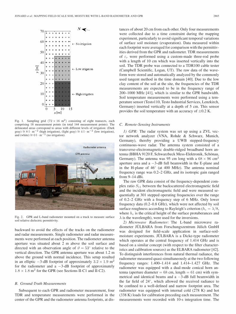
GPR, radiometer, and TDR data were collected on a 72×16 m2 experimental plot located in the upper part of the test site(Fig. 1). This plot consists of eight transects, each consistingof 18 measurement points (measurement spacing: 2 and 4 m inthe x- and y-direction, respectively). In order to produce a widerange of water contents, the plot was partially irrigated withdifferent quantities of water in two different areas using a firehose one day before the experiment. Fig. 1 shows the locationof the irrigated area. The dark-gray area was irrigated withapproximately 8 l · m−2, while the light-gray area was irrigatedwith approximately 4 l · m−2.

Measurements were performed with a radiometer and a GPRmounted on the back of a truck (see Fig. 2). The truck moved

JONARD et al.: MAPPING FIELD-SCALE SOIL MOISTURE WITH L-BAND RADIOMETER AND GPR 2865

Fig. 1. Sampling grid (72× 16 m2) consisting of eight transects, eachcomprising 18 measurement points (in total 144 measurement points). Thedelineated areas correspond to areas with different levels of irrigation: (Darkgray) ∼= 8 l · m−2 (high irrigation), (light gray) ∼= 4 l · m−2 (low irrigation),and (white) ∼= 0 l · m−2 (no irrigation).

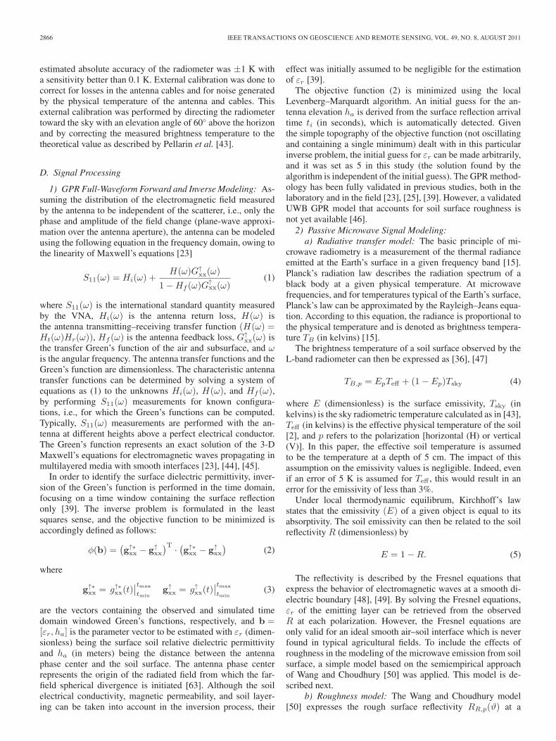
Fig. 2. GPR and L-band radiometer mounted on a truck to measure surfacesoil relative dielectric permittivity.

backward to avoid the effects of the tracks on the radiometerand radar measurements. Single radiometer and radar measure-ments were performed at each position. The radiometer antennaaperture was situated about 2 m above the soil surface anddirected with an observation angle of ϑ = 53◦ relative to thevertical direction. The GPR antenna aperture was about 1.2 mabove the ground with normal incidence. This setup resultedin an elliptic −3-dB footprint of approximately 3.2× 1.9 m2

for the radiometer and a −3-dB footprint of approximately1.8× 1.8 m2 for the GPR (see Sections II-C1 and II-C2).

B. Ground-Truth Measurements

Subsequent to each GPR and radiometer measurement, fourTDR and temperature measurements were performed in thecenter of the GPR and the radiometer antenna footprints, at dis-

tances of about 20 cm from each other. Only four measurementswere collected due to a time constraint during the mappingexperiment, particularly to avoid significant temporal variationsof surface soil moisture (evaporation). Data measured withineach footprint were averaged for comparison with the permittiv-ities derived from the GPR and radiometer. TDR measurementsof εr were performed using a custom-made three-rod probewith a length of 10 cm which was inserted vertically into thesoil. The TDR probe was connected to a TDR100 cable tester(Campbell Scientific, Logan, UT). The raw data of the wave-form were stored and automatically analyzed by the commonlyused tangent method in the time domain [40]. Due to the lowclay content of the soil at the site, the frequencies of the TDRmeasurements are expected to be in the frequency range of200–1000 MHz [41], which is similar to the GPR bandwidth.Soil temperature measurements were performed using a tem-perature sensor (Testo110, Testo Industrial Services, Lenzkirch,Germany) inserted vertically at a depth of 5 cm. This sensorprovides the soil temperature with an accuracy of ±0.2 K.

C. Remote-Sensing Instruments

1) GPR: The radar system was set up using a ZVL vec-tor network analyzer (VNA, Rohde & Schwarz, Munich,Germany), thereby providing a UWB stepped-frequencycontinuous-wave radar. The antenna system consisted of atransverse-electromagnetic double-ridged broadband horn an-tenna (BBHA 9120 F, Schwarzbeck Mess-Elektronik, Schönau,Germany). The antenna was 95 cm long with a 68× 96 cm2

aperture area and a −3-dB full beamwidth in the E-plane andin the H-plane of 46◦ (at 400 MHz). The antenna nominalfrequency range was 0.2–2 GHz, and its isotropic gain rangedfrom 9–14 dBi.

The raw GPR data consist of the frequency-dependent com-plex ratio S11 between the backscattered electromagnetic fieldand the incident electromagnetic field and were measured se-quentially at 301 stepped operating frequencies over the rangeof 0.2–2 GHz with a frequency step of 6 MHz. Only lowerfrequency data (0.2–0.8 GHz), which were not affected by soilsurface roughness according to Rayleigh’s criterion (hc = λ/8,where hc is the critical height of the surface protuberances andλ is the wavelength), were used for the inversions.

2) Microwave Radiometer: The L-band microwave ra-diometer JÜLBARA from Forschungszentrum Jülich GmbHwas designed for field-scale application in surface-soil-moisture experiments. JÜLBARA is a Dicke-type radiometerwhich operates at the central frequency of 1.414 GHz and isbased on a similar concept (with respect to the filter character-istics and calibration sources) as the ELBARA radiometer [42].To distinguish interferences from natural thermal radiance, theradiometer measured quasi-simultaneously at the two followingfrequency ranges: 1.400–1.414 and 1.414–1.427 GHz. Theradiometer was equipped with a dual-mode conical horn an-tenna (aperture diameter = 68 cm, length = 61 cm) with sym-metrical and identical beams and a −3-dB full beamwidth inthe far field of 24◦, which allowed the received radiance tobe confined to a well-defined and narrow footprint area. Theradiometer was equipped with internal cold (278 K) and hot(338 K) loads for calibration preceding each measurement. Themeasurements were recorded with 10-s integration time. The


estimated absolute accuracy of the radiometer was ±1 K witha sensitivity better than 0.1 K. External calibration was done tocorrect for losses in the antenna cables and for noise generatedby the physical temperature of the antenna and cables. Thisexternal calibration was performed by directing the radiometertoward the sky with an elevation angle of 60◦ above the horizonand by correcting the measured brightness temperature to thetheoretical value as described by Pellarin et al. [43].

D. Signal Processing

1) GPR Full-Waveform Forward and Inverse Modeling: As-suming the distribution of the electromagnetic field measuredby the antenna to be independent of the scatterer, i.e., only thephase and amplitude of the field change (plane-wave approxi-mation over the antenna aperture), the antenna can be modeledusing the following equation in the frequency domain, owing tothe linearity of Maxwell’s equations [23]

S11(ω) = Hi(ω) +H(ω)G↑

xx(ω)

1−Hf (ω)G↑xx(ω)

(1)

where S11(ω) is the international standard quantity measuredby the VNA, Hi(ω) is the antenna return loss, H(ω) isthe antenna transmitting–receiving transfer function (H(ω) =Ht(ω)Hr(ω)), Hf (ω) is the antenna feedback loss, G↑

xx(ω) isthe transfer Green’s function of the air and subsurface, and ωis the angular frequency. The antenna transfer functions and theGreen’s function are dimensionless. The characteristic antennatransfer functions can be determined by solving a system ofequations as (1) to the unknowns Hi(ω), H(ω), and Hf (ω),by performing S11(ω) measurements for known configura-tions, i.e., for which the Green’s functions can be computed.Typically, S11(ω) measurements are performed with the an-tenna at different heights above a perfect electrical conductor.The Green’s function represents an exact solution of the 3-DMaxwell’s equations for electromagnetic waves propagating inmultilayered media with smooth interfaces [23], [44], [45].

In order to identify the surface dielectric permittivity, inver-sion of the Green’s function is performed in the time domain,focusing on a time window containing the surface reflectiononly [39]. The inverse problem is formulated in the leastsquares sense, and the objective function to be minimized isaccordingly defined as follows:

φ(b) =(g↑∗xx − g↑

xx

)T ·(g↑∗xx − g↑

xx

)(2)

where

g↑∗xx = g↑∗xx(t)

∣∣tmax

tming↑xx = g↑xx(t)

∣∣tmax

tmin(3)

are the vectors containing the observed and simulated timedomain windowed Green’s functions, respectively, and b =[εr, ha] is the parameter vector to be estimated with εr (dimen-sionless) being the surface soil relative dielectric permittivityand ha (in meters) being the distance between the antennaphase center and the soil surface. The antenna phase centerrepresents the origin of the radiated field from which the far-field spherical divergence is initiated [63]. Although the soilelectrical conductivity, magnetic permeability, and soil layer-ing can be taken into account in the inversion process, their

effect was initially assumed to be negligible for the estimationof εr [39].

The objective function (2) is minimized using the localLevenberg–Marquardt algorithm. An initial guess for the an-tenna elevation ha is derived from the surface reflection arrivaltime ti (in seconds), which is automatically detected. Giventhe simple topography of the objective function (not oscillatingand containing a single minimum) dealt with in this particularinverse problem, the initial guess for εr can be made arbitrarily,and it was set as 5 in this study (the solution found by thealgorithm is independent of the initial guess). The GPR method-ology has been fully validated in previous studies, both in thelaboratory and in the field [23], [25], [39]. However, a validatedUWB GPR model that accounts for soil surface roughness isnot yet available [46].

2) Passive Microwave Signal Modeling:a) Radiative transfer model: The basic principle of mi-

crowave radiometry is a measurement of the thermal radianceemitted at the Earth’s surface in a given frequency band [15].Planck’s radiation law describes the radiation spectrum of ablack body at a given physical temperature. At microwavefrequencies, and for temperatures typical of the Earth’s surface,Planck’s law can be approximated by the Rayleigh–Jeans equa-tion. According to this equation, the radiance is proportional tothe physical temperature and is denoted as brightness tempera-ture TB (in kelvins) [15].

The brightness temperature of a soil surface observed by theL-band radiometer can then be expressed as [36], [47]

TB,p = EpTeff + (1− Ep)Tsky (4)

where E (dimensionless) is the surface emissivity, Tsky (inkelvins) is the sky radiometric temperature calculated as in [43],Teff (in kelvins) is the effective physical temperature of the soil[2], and p refers to the polarization [horizontal (H) or vertical(V)]. In this paper, the effective soil temperature is assumedto be the temperature at a depth of 5 cm. The impact of thisassumption on the emissivity values is negligible. Indeed, evenif an error of 5 K is assumed for Teff , this would result in anerror for the emissivity of less than 3%.

Under local thermodynamic equilibrum, Kirchhoff’s lawstates that the emissivity (E) of a given object is equal to itsabsorptivity. The soil emissivity can then be related to the soilreflectivity R (dimensionless) by

E = 1−R. (5)

The reflectivity is described by the Fresnel equations thatexpress the behavior of electromagnetic waves at a smooth di-electric boundary [48], [49]. By solving the Fresnel equations,εr of the emitting layer can be retrieved from the observedR at each polarization. However, the Fresnel equations areonly valid for an ideal smooth air–soil interface which is neverfound in typical agricultural fields. To include the effects ofroughness in the modeling of the microwave emission from soilsurface, a simple model based on the semiempirical approachof Wang and Choudhury [50] was applied. This model is de-scribed next.

b) Roughness model: The Wang and Choudhury model[50] expresses the rough surface reflectivity RR,p(ϑ) at a


Fig. 3. Flowchart representing the calibration procedure for the roughness parameters a and b of (7) for estimating the soil relative dielectric permittivity. Shadedboxes denote operators, and white boxes denote variables.

polarization p (H or V) and an incidence angle ϑ in relationto the specular reflectivity RF,p(ϑ) as

RR,p(ϑ) = [(1−Q)RF,p(ϑ) +QRF,p(ϑ)] exp (−h cos(ϑ)n)(6)

where Q is the polarization mixing factor, n expresses the angu-lar dependence of roughness, and h is the roughness parameter.

In our study, only a single incidence angle is used (ϑ = 53◦),and thus, the angular dependence of roughness will then notbe considered (n = 0). In most studies, polarization crosstalkis assumed to be negligible, and thus, Q = 0 is used [47],[51]. In (6), the roughness parameter h is generally consid-ered to be independent of polarization [47], [50]. However,various studies have pointed out that the roughness affects thetwo polarizations differently as a result of the anisotropy ofthe effective permittivity εr in the air to soil transition zone[52], [53]. Several studies have also shown that the roughnesseffect might change with soil moisture. Wigneron et al. [47],Schwank and Mätzler [54], and Escorihuela et al. [55] didindeed observe a negative correlation between their estimatedroughness parameter and the surface soil moisture. The appar-ently increasing roughness with decreasing soil moisture wasexplained by an increase of the dielectric heterogeneity (dielec-tric roughness) as the soil dries out. However, a recent study byEscorihuela et al. [56] showed that the dependence of the soilroughness parameter on soil moisture is due to the differencebetween the L-band radiometer sensing depth and the ground-truth sampling depth used for the calibration. Based on theseassumptions, a simplified bare soil reflectivity model account-ing for roughness was derived

RR,p = RF,p exp (−(ap + bpεr)) (7)

where a and b are the soil roughness model parameters depend-ing on polarization p. Parameter b is multiplied by εr instead ofthe volumetric soil water content to avoid any inaccuracy due tothe petrophysical relationship. Given that the model parametersare determined by best fit, they include the measurements errorsand their physical meaning is not straightforward [55].

The inversion procedure adopted for the estimation of theroughness parameters is shown in Fig. 3. In this optimizationprocess, only radiometer and reference TDR data are used.Inversion is composed of two sequential optimization steps.The first inverse problem consists of solving a nonlinear leastsquares problem. In this case, the Gauss–Newton algorithm isused to minimize the objective function

Φ(εr) =∑

(R∗R −RR)

2 . (8)

This objective function represents the cumulative squared errorbetween the measured and modeled reflectivity radiometer data(R∗

R and RR(a, b), respectively). The measured reflectivity dataare obtained from the brightness temperature measurements byusing the radiative transfer model presented in (4) and (5). Theradiometer data from each polarization are used separately inthe inversion procedure to obtain specific roughness parametersfor each polarization. The second inverse problem consists inminimizing the objective function

Φ′(a, b) =∑

(ε∗r − εr)2 . (9)

The objective function Φ′ represents the cumulative squarederror between the measured and modeled dielectric permittivitydata (ε∗r and εr(a, b), respectively) and is minimized bymeans of the global multilevel coordinate search optimization


algorithm combined with the local Nelder–Mead simplex algo-rithm (GMCS-NMS, see [57]). Measured permittivity data areobtained from raw TDR data while modeled permittivity dataare obtained from the solutions of the first inverse problem. Ateach iteration, new roughness parameters are generated, whichare used in the roughness model (7) to produce new modeledreflectivity data and then new modeled dielectric permittivitydata. The optimal roughness parameters a and b are finallyobtained after numerous iterations. For the optimization conver-gence criteria, the default values of the implementation of theNelder–Mead simplex algorithm in Matlab (The MathWorksInc.) were used (i.e., termination tolerance on the functionvalue set to 10−4 and termination tolerance on the optimizedparameters set to 10−4). It has to be noted that more stringentconditions did not affect the fitting results.

E. Petrophysical Relationship

For each type of measurement (GPR, radiometer, and TDR),the model of Topp et al. [58] was used to relate the soilvolumetric water content [θ (in m3 · m−3)] to the soil relativedielectric permittivity

θ = −5.3× 10−2 + 2.92× 10−2εr − 5.5× 10−4ε2r

+ 4.3× 10−6ε3r. (10)

The Topp model is a widely used empirical relationship mainlyapplied for TDR measurements with some restrictions forhighly clayic- and organic-rich soils as well as soils withhigh bulk electrical conductivity. For our study site, Topp’smodel was shown to perform well by Weihermüller et al. [24].The authors found a root-mean-square (rms) error of0.021 m3 · m−3 between volumetric soil samples and TDRestimates.

III. RESULTS AND DISCUSSION

A. Off-Ground GPR

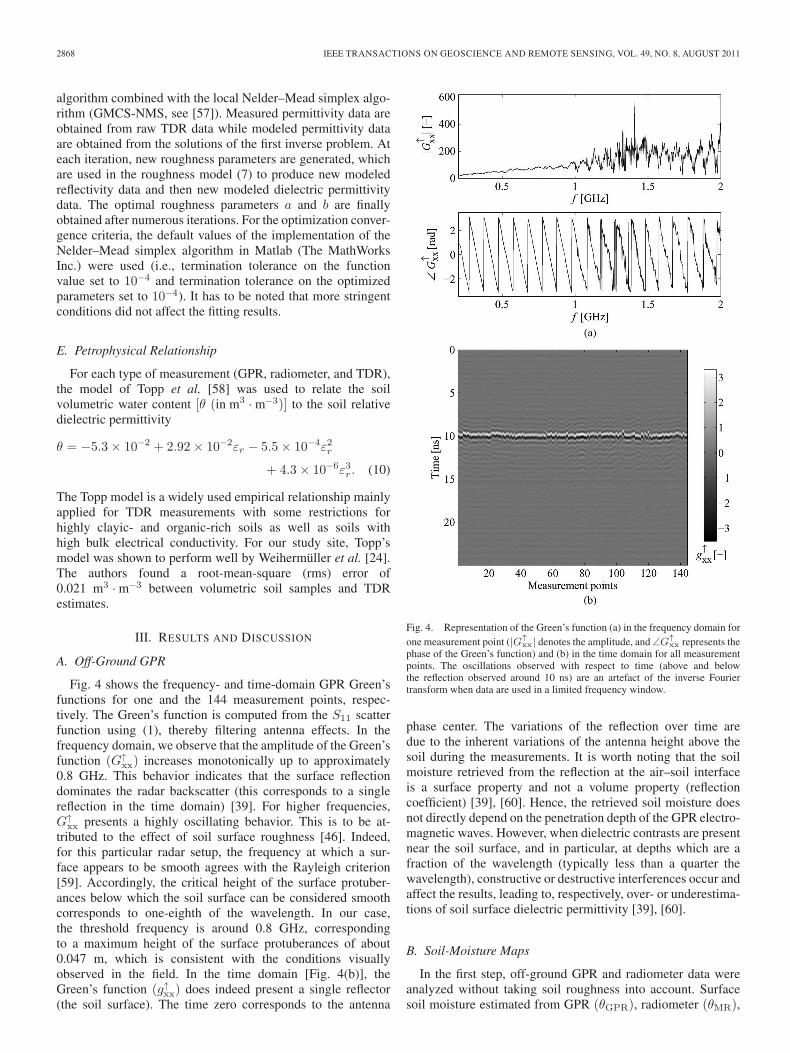
Fig. 4 shows the frequency- and time-domain GPR Green’sfunctions for one and the 144 measurement points, respec-tively. The Green’s function is computed from the S11 scatterfunction using (1), thereby filtering antenna effects. In thefrequency domain, we observe that the amplitude of the Green’sfunction (G↑

xx) increases monotonically up to approximately0.8 GHz. This behavior indicates that the surface reflectiondominates the radar backscatter (this corresponds to a singlereflection in the time domain) [39]. For higher frequencies,G↑

xx presents a highly oscillating behavior. This is to be at-tributed to the effect of soil surface roughness [46]. Indeed,for this particular radar setup, the frequency at which a sur-face appears to be smooth agrees with the Rayleigh criterion[59]. Accordingly, the critical height of the surface protuber-ances below which the soil surface can be considered smoothcorresponds to one-eighth of the wavelength. In our case,the threshold frequency is around 0.8 GHz, correspondingto a maximum height of the surface protuberances of about0.047 m, which is consistent with the conditions visuallyobserved in the field. In the time domain [Fig. 4(b)], theGreen’s function (g↑xx) does indeed present a single reflector(the soil surface). The time zero corresponds to the antenna

Fig. 4. Representation of the Green’s function (a) in the frequency domain forone measurement point (|G↑

xx| denotes the amplitude, and ∠G↑xx represents the

phase of the Green’s function) and (b) in the time domain for all measurementpoints. The oscillations observed with respect to time (above and belowthe reflection observed around 10 ns) are an artefact of the inverse Fouriertransform when data are used in a limited frequency window.

phase center. The variations of the reflection over time aredue to the inherent variations of the antenna height above thesoil during the measurements. It is worth noting that the soilmoisture retrieved from the reflection at the air–soil interfaceis a surface property and not a volume property (reflectioncoefficient) [39], [60]. Hence, the retrieved soil moisture doesnot directly depend on the penetration depth of the GPR electro-magnetic waves. However, when dielectric contrasts are presentnear the soil surface, and in particular, at depths which are afraction of the wavelength (typically less than a quarter thewavelength), constructive or destructive interferences occur andaffect the results, leading to, respectively, over- or underestima-tions of soil surface dielectric permittivity [39], [60].

B. Soil-Moisture Maps

In the first step, off-ground GPR and radiometer data wereanalyzed without taking soil roughness into account. Surfacesoil moisture estimated from GPR (θGPR), radiometer (θMR),


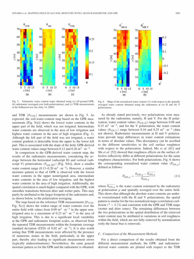
Fig. 5. Volumetric water content maps obtained using (a) off-ground GPR,(b) radiometer (averaged over both polarizations), and (c) TDR measurementsat the Selhausen test site (July 14, 2009).

and TDR (θTDR) measurements are shown in Fig. 5. Asexpected, the soil-water-content map based on the GPR mea-surements [Fig. 5(a)] shows the lowest water contents in theupper part of the field, which was not irrigated. Intermediatewater contents are observed in the area of low irrigation andhighest water contents in the area of high irrigation (Fig. 1).Although the left part of the field was not irrigated, a watercontent gradient is detectable from the upper to the lower leftpart. This is associated with the slope of the field. GPR-derivedwater content values range between 0.12 and 0.26 m3 · m−3.

In comparison to the GPR-derived water content map, theresults of the radiometer measurements, considering the av-erage between the horizontal (subscript H) and vertical (sub-script V) polarizations (θMR,HV) [Fig. 5(b)], show a smallerwater content range (0.13–0.20 m3 · m−3). However, a similarmoisture pattern to that of GPR is observed with the lowestwater contents in the upper nonirrigated area, intermediatewater contents in the area of low irrigation, and the highestwater contents in the area of high irrigation. Additionally, thespatial correlation is much higher compared with the GPR, withsmoother transitions between drier and wetter parts. This maypartly be attributed to the larger footprint of the radiometer and,as shown below, to the polarization averaging.

The map based on the reference TDR measurements [θTDR,Fig. 5(c)] shows the widest range of water contents over theentire field with values from 0.09 m3 · m−3 in the upper non-irrigated area to a maximum of 0.23 m3 · m−3 in the area ofhigh irrigation. This is due to a significant local variabilityat the GPR and radiometer footprint scales, as observed fromthe repeated TDR measurements within the footprints (averagestandard deviation (STD) of 0.02 m3 · m−3). It is also worthnoting that TDR measurements were affected by the presenceof numerous stones in the field, particularly in the upperpart, thereby also leading to significant measurement errors(typically underestimations). Nevertheless, the same generalmoisture pattern as for the GPR and the radiometer is obtained.

Fig. 6. Maps of the normalized water content (11) with respect to the spatiallyaveraged water content obtained using the radiometer at (a) H and (b) Vpolarizations.

As already stated previously, two polarizations were mea-sured by the radiometer, namely, H and V. For the H polar-ization, water content values (θMR,H) range between 0.08 and0.15 m3 · m−3, and for the V polarization, the water contentvalues (θMR,V) range between 0.16 and 0.25 m3 · m−3 (datanot shown). Radiometer measurements at H and V polariza-tions provide large differences in water content estimationsin terms of absolute values. This discrepancy can be ascribedto the different sensitivities to the soil surface roughnesswith respect to the polarization. Indeed, Mo et al. [61] andShi et al. [52] showed that roughness effects on the surface ef-fective reflectivity differ at different polarizations for the sameroughness characteristics. For both polarizations, Fig. 6 showsthe corresponding normalized water content value (θ∗MR,p)defined as follows:

θ∗MR,p =θMR,p − θMR,p

θMR,p

(11)

where θMR,p is the water content estimated by the radiometerat polarization p and spatially averaged over the entire field.This shows that although the absolute water contents are under-or overestimated with the H and V polarizations, the spatialpattern is similar for the two normalized maps (correlation coef-ficient r2 = 0.74) and consistent with the GPR and TDR maps(wetter and drier zones). The remaining differences betweenthe two polarizations in the spatial distribution of the retrievedwater content may be attributed to variations in soil roughnesswithin the field, which are not fully removed by normalization(only the linear bias is removed).

C. Comparison of the Measurement Methods

For a direct comparison of the results obtained from thedifferent measurement methods, the GPR- and radiometer-derived water contents are plotted with respect to the TDR


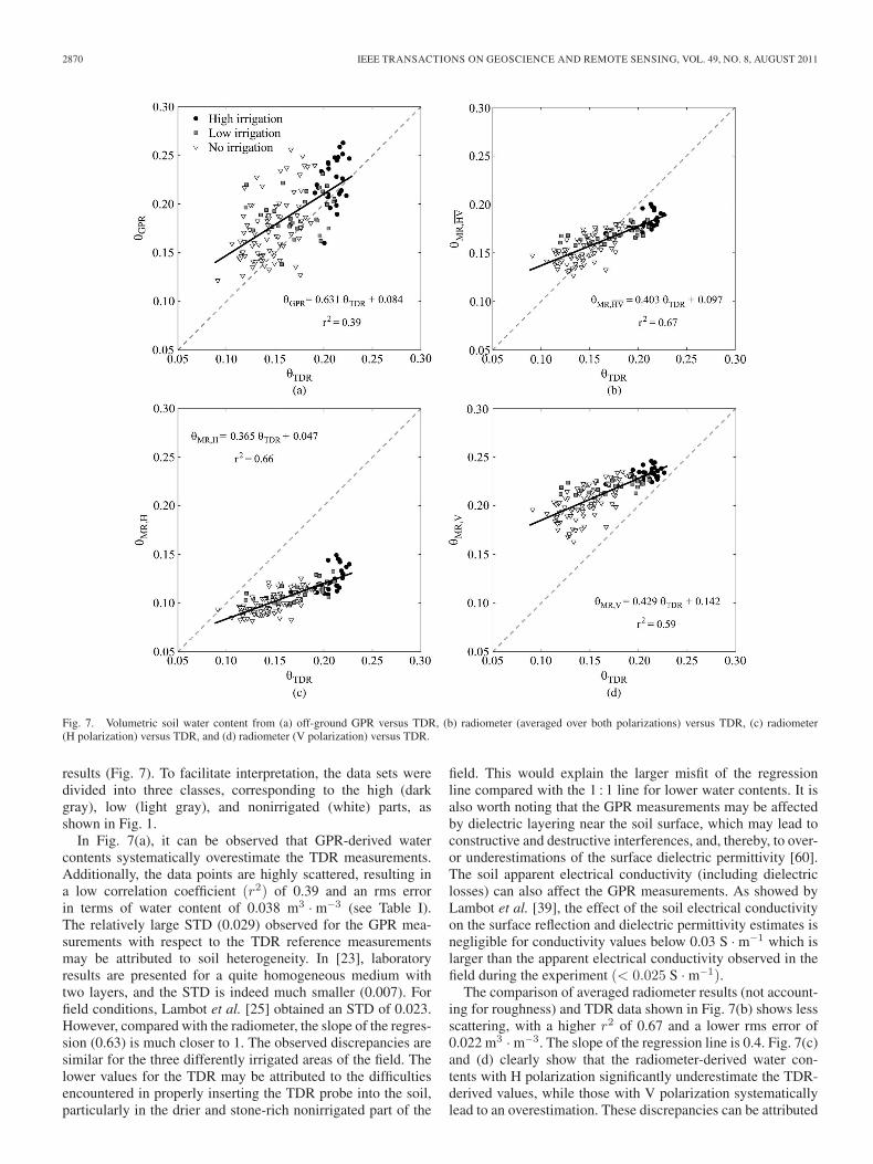
Fig. 7. Volumetric soil water content from (a) off-ground GPR versus TDR, (b) radiometer (averaged over both polarizations) versus TDR, (c) radiometer(H polarization) versus TDR, and (d) radiometer (V polarization) versus TDR.

results (Fig. 7). To facilitate interpretation, the data sets weredivided into three classes, corresponding to the high (darkgray), low (light gray), and nonirrigated (white) parts, asshown in Fig. 1.

In Fig. 7(a), it can be observed that GPR-derived watercontents systematically overestimate the TDR measurements.Additionally, the data points are highly scattered, resulting ina low correlation coefficient (r2) of 0.39 and an rms errorin terms of water content of 0.038 m3 · m−3 (see Table I).The relatively large STD (0.029) observed for the GPR mea-surements with respect to the TDR reference measurementsmay be attributed to soil heterogeneity. In [23], laboratoryresults are presented for a quite homogeneous medium withtwo layers, and the STD is indeed much smaller (0.007). Forfield conditions, Lambot et al. [25] obtained an STD of 0.023.However, compared with the radiometer, the slope of the regres-sion (0.63) is much closer to 1. The observed discrepancies aresimilar for the three differently irrigated areas of the field. Thelower values for the TDR may be attributed to the difficultiesencountered in properly inserting the TDR probe into the soil,particularly in the drier and stone-rich nonirrigated part of the

field. This would explain the larger misfit of the regressionline compared with the 1 : 1 line for lower water contents. It isalso worth noting that the GPR measurements may be affectedby dielectric layering near the soil surface, which may lead toconstructive and destructive interferences, and, thereby, to over-or underestimations of the surface dielectric permittivity [60].The soil apparent electrical conductivity (including dielectriclosses) can also affect the GPR measurements. As showed byLambot et al. [39], the effect of the soil electrical conductivityon the surface reflection and dielectric permittivity estimates isnegligible for conductivity values below 0.03 S · m−1 which islarger than the apparent electrical conductivity observed in thefield during the experiment (< 0.025 S · m−1).

The comparison of averaged radiometer results (not account-ing for roughness) and TDR data shown in Fig. 7(b) shows lessscattering, with a higher r2 of 0.67 and a lower rms error of0.022 m3 · m−3. The slope of the regression line is 0.4. Fig. 7(c)and (d) clearly show that the radiometer-derived water con-tents with H polarization significantly underestimate the TDR-derived values, while those with V polarization systematicallylead to an overestimation. These discrepancies can be attributed


TABLE IDIAGONAL MATRICES OF RMS ERROR IN TERMS OF WATER CONTENT (RMS ERROR θ) AND RELATIVE DIELECTRIC PERMITTIVITY (RMS ERROR εr)FOR THE GPR-, TDR-, AND RADIOMETER-AVERAGED (HV-POL), HORIZONTAL (H-POL), AND VERTICAL (V-POL) POLARIZATIONS, RESPECTIVELY

to the different sensitivities of the two polarizations with respectto roughness. In general, the H polarization better predicts thelower water contents in the nonirrigated areas compared withthe higher water contents from the irrigated parts. Indeed, inFig. 7(c), the low-water-content data are closer to the 1 : 1line compared with the higher water content data, whereasthe opposite is observed in Fig. 7(d). However, the r2 is still0.66 m3 · m−3 for the H polarization and 0.59 m3 · m−3 forthe V polarization, respectively, whereby the high rms errorsof 0.062 and 0.054 m3 · m−3 clearly indicate the systematicalmismatch between the two techniques. This explains the smallrms error obtained by averaging the two polarizations.

The frequency dependence of the soil dielectric permittivityover the frequency range covered by the three methods (GPR,radiometer, and TDR) is expected to be rather small [23] asall methods operate at frequencies well below the relaxationfrequency of free water (approximately 16 GHz). However, asthe soil is inherently heterogeneous, differences in soil moistureretrieved by the three techniques can also be partly explained bythe different characterized soil volumes.

D. Accounting for Soil Surface Roughness for the Radiometer

As already stated, soil surface roughness plays an importantrole in the retrieval of soil water content from the radiometerdata. In this section, soil surface roughness is accounted forusing the empirical roughness model [see (7)]. The optimalroughness parameters obtained by the inversion scheme inFig. 3 are a = 0.1818 and b = 0.0013 for the H polarizationand a = −1.1480 and b = 0.0913 for the V polarization, re-spectively. The value of b is close to zero for the H polarization,which means that the model dependence on εr is negligible forthis polarization. It is worth noting that, as they are empirical,no constraint on the value of the estimated parameters duringthe inversion process was applied and their physical meaning isnot straightforward. The values of these parameters depend onall electromagnetic phenomena that are not properly accountedfor by the Fresnel model, particularly roughness effects, andmeasurement errors.

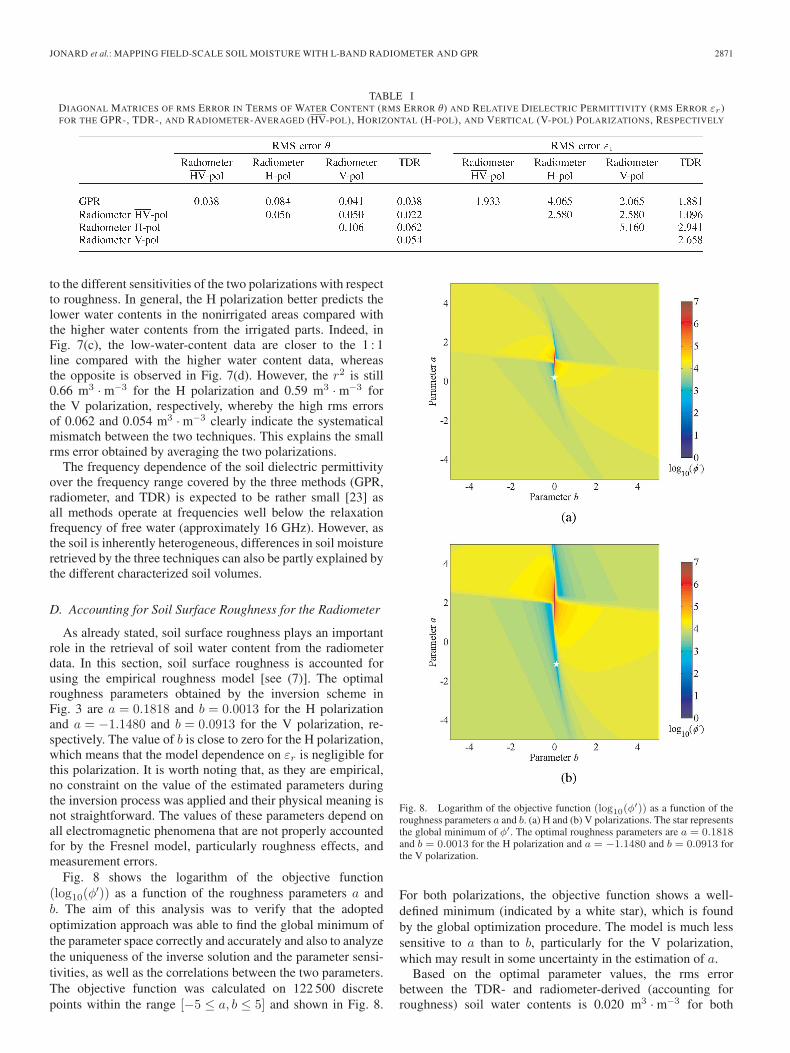
Fig. 8 shows the logarithm of the objective function(log10(φ

′)) as a function of the roughness parameters a andb. The aim of this analysis was to verify that the adoptedoptimization approach was able to find the global minimum ofthe parameter space correctly and accurately and also to analyzethe uniqueness of the inverse solution and the parameter sensi-tivities, as well as the correlations between the two parameters.The objective function was calculated on 122 500 discretepoints within the range [−5 ≤ a, b ≤ 5] and shown in Fig. 8.

Fig. 8. Logarithm of the objective function (log10(φ′)) as a function of the

roughness parameters a and b. (a) H and (b) V polarizations. The star representsthe global minimum of φ′. The optimal roughness parameters are a = 0.1818and b = 0.0013 for the H polarization and a = −1.1480 and b = 0.0913 forthe V polarization.

For both polarizations, the objective function shows a well-defined minimum (indicated by a white star), which is foundby the global optimization procedure. The model is much lesssensitive to a than to b, particularly for the V polarization,which may result in some uncertainty in the estimation of a.

Based on the optimal parameter values, the rms errorbetween the TDR- and radiometer-derived (accounting forroughness) soil water contents is 0.020 m3 · m−3 for both


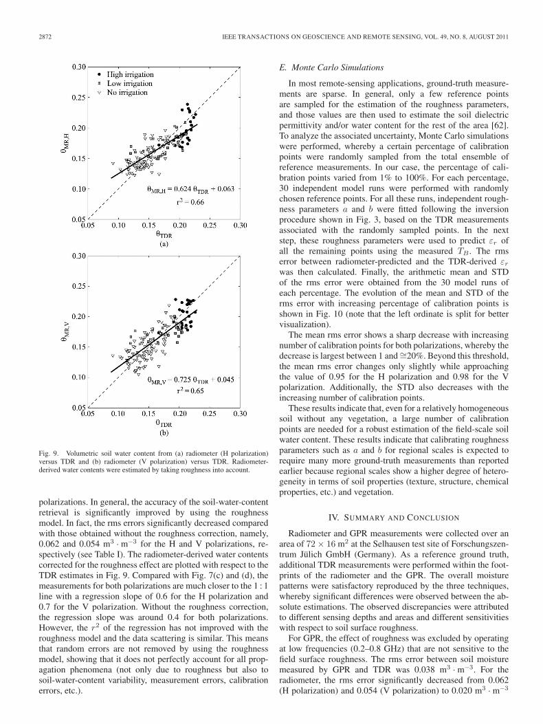
Fig. 9. Volumetric soil water content from (a) radiometer (H polarization)versus TDR and (b) radiometer (V polarization) versus TDR. Radiometer-derived water contents were estimated by taking roughness into account.

polarizations. In general, the accuracy of the soil-water-contentretrieval is significantly improved by using the roughnessmodel. In fact, the rms errors significantly decreased comparedwith those obtained without the roughness correction, namely,0.062 and 0.054 m3 · m−3 for the H and V polarizations, re-spectively (see Table I). The radiometer-derived water contentscorrected for the roughness effect are plotted with respect to theTDR estimates in Fig. 9. Compared with Fig. 7(c) and (d), themeasurements for both polarizations are much closer to the 1 : 1line with a regression slope of 0.6 for the H polarization and0.7 for the V polarization. Without the roughness correction,the regression slope was around 0.4 for both polarizations.However, the r2 of the regression has not improved with theroughness model and the data scattering is similar. This meansthat random errors are not removed by using the roughnessmodel, showing that it does not perfectly account for all prop-agation phenomena (not only due to roughness but also tosoil-water-content variability, measurement errors, calibrationerrors, etc.).

E. Monte Carlo Simulations

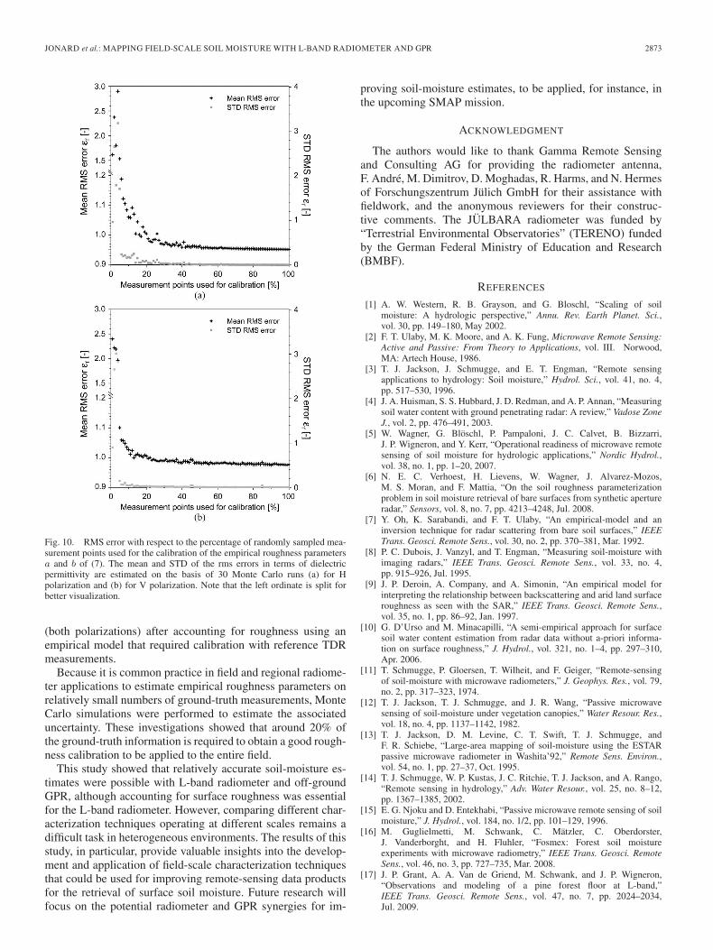
In most remote-sensing applications, ground-truth measure-ments are sparse. In general, only a few reference pointsare sampled for the estimation of the roughness parameters,and those values are then used to estimate the soil dielectricpermittivity and/or water content for the rest of the area [62].To analyze the associated uncertainty, Monte Carlo simulationswere performed, whereby a certain percentage of calibrationpoints were randomly sampled from the total ensemble ofreference measurements. In our case, the percentage of cali-bration points varied from 1% to 100%. For each percentage,30 independent model runs were performed with randomlychosen reference points. For all these runs, independent rough-ness parameters a and b were fitted following the inversionprocedure shown in Fig. 3, based on the TDR measurementsassociated with the randomly sampled points. In the nextstep, these roughness parameters were used to predict εr ofall the remaining points using the measured TB . The rmserror between radiometer-predicted and the TDR-derived εrwas then calculated. Finally, the arithmetic mean and STDof the rms error were obtained from the 30 model runs ofeach percentage. The evolution of the mean and STD of therms error with increasing percentage of calibration points isshown in Fig. 10 (note that the left ordinate is split for bettervisualization).

The mean rms error shows a sharp decrease with increasingnumber of calibration points for both polarizations, whereby thedecrease is largest between 1 and ∼=20%. Beyond this threshold,the mean rms error changes only slightly while approachingthe value of 0.95 for the H polarization and 0.98 for the Vpolarization. Additionally, the STD also decreases with theincreasing number of calibration points.

These results indicate that, even for a relatively homogeneoussoil without any vegetation, a large number of calibrationpoints are needed for a robust estimation of the field-scale soilwater content. These results indicate that calibrating roughnessparameters such as a and b for regional scales is expected torequire many more ground-truth measurements than reportedearlier because regional scales show a higher degree of hetero-geneity in terms of soil properties (texture, structure, chemicalproperties, etc.) and vegetation.

IV. SUMMARY AND CONCLUSION

Radiometer and GPR measurements were collected over anarea of 72× 16 m2 at the Selhausen test site of Forschungszen-trum Jülich GmbH (Germany). As a reference ground truth,additional TDR measurements were performed within the foot-prints of the radiometer and the GPR. The overall moisturepatterns were satisfactory reproduced by the three techniques,whereby significant differences were observed between the ab-solute estimations. The observed discrepancies were attributedto different sensing depths and areas and different sensitivitieswith respect to soil surface roughness.

For GPR, the effect of roughness was excluded by operatingat low frequencies (0.2–0.8 GHz) that are not sensitive to thefield surface roughness. The rms error between soil moisturemeasured by GPR and TDR was 0.038 m3 · m−3. For theradiometer, the rms error significantly decreased from 0.062(H polarization) and 0.054 (V polarization) to 0.020 m3 · m−3


Fig. 10. RMS error with respect to the percentage of randomly sampled mea-surement points used for the calibration of the empirical roughness parametersa and b of (7). The mean and STD of the rms errors in terms of dielectricpermittivity are estimated on the basis of 30 Monte Carlo runs (a) for Hpolarization and (b) for V polarization. Note that the left ordinate is split forbetter visualization.

(both polarizations) after accounting for roughness using anempirical model that required calibration with reference TDRmeasurements.

Because it is common practice in field and regional radiome-ter applications to estimate empirical roughness parameters onrelatively small numbers of ground-truth measurements, MonteCarlo simulations were performed to estimate the associateduncertainty. These investigations showed that around 20% ofthe ground-truth information is required to obtain a good rough-ness calibration to be applied to the entire field.

This study showed that relatively accurate soil-moisture es-timates were possible with L-band radiometer and off-groundGPR, although accounting for surface roughness was essentialfor the L-band radiometer. However, comparing different char-acterization techniques operating at different scales remains adifficult task in heterogeneous environments. The results of thisstudy, in particular, provide valuable insights into the develop-ment and application of field-scale characterization techniquesthat could be used for improving remote-sensing data productsfor the retrieval of surface soil moisture. Future research willfocus on the potential radiometer and GPR synergies for im-

proving soil-moisture estimates, to be applied, for instance, inthe upcoming SMAP mission.

ACKNOWLEDGMENT

The authors would like to thank Gamma Remote Sensingand Consulting AG for providing the radiometer antenna,F. André, M. Dimitrov, D. Moghadas, R. Harms, and N. Hermesof Forschungszentrum Jülich GmbH for their assistance withfieldwork, and the anonymous reviewers for their construc-tive comments. The JÜLBARA radiometer was funded by“Terrestrial Environmental Observatories” (TERENO) fundedby the German Federal Ministry of Education and Research(BMBF).

REFERENCES

[1] A. W. Western, R. B. Grayson, and G. Bloschl, “Scaling of soilmoisture: A hydrologic perspective,” Annu. Rev. Earth Planet. Sci.,vol. 30, pp. 149–180, May 2002.

[2] F. T. Ulaby, M. K. Moore, and A. K. Fung, Microwave Remote Sensing:Active and Passive: From Theory to Applications, vol. III. Norwood,MA: Artech House, 1986.

[3] T. J. Jackson, J. Schmugge, and E. T. Engman, “Remote sensingapplications to hydrology: Soil moisture,” Hydrol. Sci., vol. 41, no. 4,pp. 517–530, 1996.

[4] J. A. Huisman, S. S. Hubbard, J. D. Redman, and A. P. Annan, “Measuringsoil water content with ground penetrating radar: A review,” Vadose ZoneJ., vol. 2, pp. 476–491, 2003.

[5] W. Wagner, G. Blöschl, P. Pampaloni, J. C. Calvet, B. Bizzarri,J. P. Wigneron, and Y. Kerr, “Operational readiness of microwave remotesensing of soil moisture for hydrologic applications,” Nordic Hydrol.,vol. 38, no. 1, pp. 1–20, 2007.

[6] N. E. C. Verhoest, H. Lievens, W. Wagner, J. Alvarez-Mozos,M. S. Moran, and F. Mattia, “On the soil roughness parameterizationproblem in soil moisture retrieval of bare surfaces from synthetic apertureradar,” Sensors, vol. 8, no. 7, pp. 4213–4248, Jul. 2008.

[7] Y. Oh, K. Sarabandi, and F. T. Ulaby, “An empirical-model and aninversion technique for radar scattering from bare soil surfaces,” IEEETrans. Geosci. Remote Sens., vol. 30, no. 2, pp. 370–381, Mar. 1992.

[8] P. C. Dubois, J. Vanzyl, and T. Engman, “Measuring soil-moisture withimaging radars,” IEEE Trans. Geosci. Remote Sens., vol. 33, no. 4,pp. 915–926, Jul. 1995.

[9] J. P. Deroin, A. Company, and A. Simonin, “An empirical model forinterpreting the relationship between backscattering and arid land surfaceroughness as seen with the SAR,” IEEE Trans. Geosci. Remote Sens.,vol. 35, no. 1, pp. 86–92, Jan. 1997.

[10] G. D’Urso and M. Minacapilli, “A semi-empirical approach for surfacesoil water content estimation from radar data without a-priori informa-tion on surface roughness,” J. Hydrol., vol. 321, no. 1–4, pp. 297–310,Apr. 2006.

[11] T. Schmugge, P. Gloersen, T. Wilheit, and F. Geiger, “Remote-sensingof soil-moisture with microwave radiometers,” J. Geophys. Res., vol. 79,no. 2, pp. 317–323, 1974.

[12] T. J. Jackson, T. J. Schmugge, and J. R. Wang, “Passive microwavesensing of soil-moisture under vegetation canopies,” Water Resour. Res.,vol. 18, no. 4, pp. 1137–1142, 1982.

[13] T. J. Jackson, D. M. Levine, C. T. Swift, T. J. Schmugge, andF. R. Schiebe, “Large-area mapping of soil-moisture using the ESTARpassive microwave radiometer in Washita’92,” Remote Sens. Environ.,vol. 54, no. 1, pp. 27–37, Oct. 1995.

[14] T. J. Schmugge, W. P. Kustas, J. C. Ritchie, T. J. Jackson, and A. Rango,“Remote sensing in hydrology,” Adv. Water Resour., vol. 25, no. 8–12,pp. 1367–1385, 2002.

[15] E. G. Njoku and D. Entekhabi, “Passive microwave remote sensing of soilmoisture,” J. Hydrol., vol. 184, no. 1/2, pp. 101–129, 1996.

[16] M. Guglielmetti, M. Schwank, C. Mätzler, C. Oberdorster,J. Vanderborght, and H. Fluhler, “Fosmex: Forest soil moistureexperiments with microwave radiometry,” IEEE Trans. Geosci. RemoteSens., vol. 46, no. 3, pp. 727–735, Mar. 2008.

[17] J. P. Grant, A. A. Van de Griend, M. Schwank, and J. P. Wigneron,“Observations and modeling of a pine forest floor at L-band,”IEEE Trans. Geosci. Remote Sens., vol. 47, no. 7, pp. 2024–2034,Jul. 2009.


[18] J. S. Famiglietti, J. A. Devereaux, C. A. Laymon, T. Tsegaye, P. R. Houser,T. J. Jackson, S. T. Graham, M. Rodell, and P. J. van Oevelen, “Ground-based investigation of soil moisture variability within remote sensingfootprints during the southern great plains 1997 (SGP97) hydrologyexperiment,” Water Resour. Res., vol. 35, no. 6, pp. 1839–1851,1999.

[19] A. P. Annan, “GPR methods for hydrogeological studies,” in Hydrogeo-physics, Y. Rubin and S. Hubbard, Eds. New York: Springer-Verlag,2005, pp. 185–213.

[20] J. R. Ernst, K. Holliger, H. Maurer, and A. G. Green, “RealisticFDTD modelling of borehole georadar antenna radiation: Methodol-ogy and application,” Near Surf. Geophys., vol. 4, no. 1, pp. 19–30,2006.

[21] E. Gloaguen, B. Giroux, D. Marcotte, and R. Dimitrakopoulos,“Pseudo-full-waveform inversion of borehole GPR data using stochastictomography,” Geophysics, vol. 72, no. 5, pp. J43–J51, Sep./Oct. 2007.

[22] F. Soldovieri, J. Hugenschmidt, R. Persico, and G. Leone, “A linearinverse scattering algorithm for realistic GPR applications,” Near Surf.Geophys., vol. 5, no. 1, pp. 29–41, 2007.

[23] S. Lambot, E. C. Slob, I. van den Bosch, B. Stockbroeckx, andM. Vanclooster, “Modeling of ground-penetrating radar for accuratecharacterization of subsurface electric properties,” IEEE Trans. Geosci.Remote Sens., vol. 42, no. 11, pp. 2555–2568, Nov. 2004.

[24] L. Weihermüller, J. A. Huisman, S. Lambot, M. Herbst, and H. Vereecken,“Mapping the spatial variation of soil water content at the field scalewith different ground penetrating radar techniques,” J. Hydrol., vol. 340,no. 3/4, pp. 205–216, Jul. 2007.

[25] S. Lambot, E. Slob, D. Chavarro, M. Lubczynski, and H. Vereecken,“Measuring soil surface water content in irrigated areas of SouthernTunisia using full-waveform inversion of proximal GPR data,” Near Surf.Geophys., vol. 6, pp. 403–410, 2008.

[26] P. Ferrazzoli, S. Paloscia, P. Pampaloni, G. Schiavon, D. Solimini,and P. Coppo, “Sensitivity of microwave measurements to vegetationbiomass and soil-moisture content—A case-study,” IEEE Trans. Geosci.Remote Sens., vol. 30, no. 4, pp. 750–756, Jul. 1992.

[27] K. Saleh, J. P. Wigneron, P. Waldteufel, P. de Rosnay, M. Schwank,J. C. Calvet, and Y. H. Kerr, “Estimates of surface soil moisture undergrass covers using L-band radiometry,” Remote Sens. Environ., vol. 109,no. 1, pp. 42–53, Jul. 2007.

[28] J. P. Wigneron, Y. Kerr, P. Waldteufel, K. Saleh, M. J. Escorihuela,P. Richaume, P. Ferrazzoli, P. de Rosnay, R. Gurney, J. C. Calvet,J. P. Grant, M. Guglielmetti, B. Hornbuckle, C. Mätzler, T. Pellarin, andM. Schwank, “L-band Microwave Emission of the Biosphere (L-MEB)model: Description and calibration against experimental data sets overcrop fields,” Remote Sens. Environ., vol. 107, no. 4, pp. 639–655,Apr. 2007.

[29] M. Schwank, M. Guglielmetti, C. Mätzler, and H. Fluhler, “Testing a newmodel for the L-band radiation of moist leaf litter,” IEEE Trans. Geosci.Remote Sens., vol. 46, no. 7, pp. 1982–1994, Jul. 2008.

[30] B. J. Choudhury, T. J. Schmugge, and T. Mo, “A parameterization ofeffective soil-temperature for microwave emission,” J. Geophys. Res.,vol. 87, no. C2, pp. 1301–1304, 1982.

[31] A. Chanzy, S. Raju, and J. P. Wigneron, “Estimation of soil microwaveeffective temperature at L and C bands,” IEEE Trans. Geosci. RemoteSens., vol. 35, no. 3, pp. 570–580, May 1997.

[32] B. J. Choudhury, T. J. Schmugge, A. Chang, and R. W. Newton, “Effectof surface-roughness on the microwave emission from soils,” J. Geophys.Res., vol. 84, no. C9, pp. 5699–5706, 1979.

[33] T. Mo and T. J. Schmugge, “A parameterization of the effect of surface-roughness on microwave emission,” IEEE Trans. Geosci. Remote Sens.,vol. GRS-25, no. 4, pp. 481–486, Jul. 1987.

[34] C. Mätzler, “Passive microwave signatures of landscapes in winter,”Meteorol. Atmos. Phys., vol. 54, no. 1–4, pp. 241–260, Mar. 1994.

[35] C. Mätzler and A. Standley, “Relief effects for passive microwave re-mote sensing,” Int. J. Remote Sens., vol. 21, no. 12, pp. 2403–2412,2000.

[36] T. J. Jackson, “Measuring surface soil-moisture using passive mi-crowave remote-sensing,” Hydrol. Process., vol. 7, no. 2, pp. 139–152,1993.

[37] J. P. Wigneron, A. Chanzy, J. C. Calvet, and W. Bruguier, “A simplealgorithm to retrieve soil-moisture and vegetation biomass using pas-sive microwave measurements over crop fields,” Remote Sens. Environ.,vol. 51, no. 3, pp. 331–341, Mar. 1995.

[38] H. Vereecken, J. A. Huisman, H. Bogena, J. Vanderborght, J. A. Vrugt,and J. W. Hopmans, “On the value of soil moisture measurements invadose zone hydrology: A review,” Water Resour. Res., vol. 44,p. W00D06, Oct. 2008.

[39] S. Lambot, L. Weihermüller, J. A. Huisman, H. Vereecken,M. Vanclooster, and E. C. Slob, “Analysis of air-launched ground-penetrating radar techniques to measure the soil surface water content,”Water Resour. Res., vol. 42, p. W11403, 2006, DOI: 11410.11029/12006WR005097.

[40] T. J. Heimovaara and W. Bouten, “A computer-controlled 36-channel timedomain reflectometry system for monitoring soil water contents,” WaterResour. Res., vol. 26, no. 10, pp. 2311–2316, 1990.

[41] D. A. Robinson, M. G. Schaap, D. Or, and S. B. Jones, “On the effectivemeasurement frequency of time domain reflectometry in dispersive andnonconductive dielectric materials,” Water Resour. Res., vol. 41, no. 2,p. W02007, Feb. 2005.

[42] C. Mätzler, D. Weber, M. Wuthrich, K. Schneeberger, C. Stamm,H. Wydler, and H. Fluhler, “ELBARA, the ETH L-band radiometer forsoil-moisture research,” in Proc. 23rd IGARSS, Toulouse, France, 2003,pp. 3058–3060.

[43] T. Pellarin, J. P. Wigneron, J. C. Calvet, M. Berger, H. Douville,P. Ferrazzoli, Y. H. Kerr, E. Lopez-Baeza, J. Pulliainen, L. P. Simmonds,and P. Waldteufel, “Two-year global simulation of L-band brightnesstemperatures over land,” IEEE Trans. Geosci. Remote Sens., vol. 41, no. 9,pp. 2135–2139, Sep. 2003.

[44] K. A. Michalski and J. R. Mosig, “Multilayered media green’s functions inintegral equation formulations,” IEEE Trans. Antennas Propag., vol. 45,no. 3, pp. 508–519, Mar. 1997.

[45] E. C. Slob and J. Fokkema, “Coupling effects of two electric dipoleson an interface,” Radio Sci., vol. 37, no. 5, p. 1073, Sep. 2002, DOI:1010.1029/2001RS002529.

[46] S. Lambot, M. Antoine, M. Vanclooster, and E. C. Slob, “Effect of soilroughness on the inversion of off-ground monostatic GPR signal fornoninvasive quantification of soil properties,” Water Resour. Res., vol. 42,p. W03403, 2006, DOI: 03410.01029/02005WR004416.

[47] J. P. Wigneron, L. Laguerre, and Y. H. Kerr, “A simple parameteriza-tion of the L-band microwave emission from rough agricultural soils,”IEEE Trans. Geosci. Remote Sens., vol. 39, no. 8, pp. 1697–1707,Aug. 2001.

[48] F. T. Ulaby, M. K. Moore, and A. K. Fung, Microwave Remote Sensing:Active and Passive: Fundamentals and Radiometry, vol. I. Boston, MA:Addison Wesley, 1981.

[49] J. A. Kong, Electromagnetic Wave Theory, 2nd ed. New York: Wiley,1990.

[50] J. R. Wang and B. J. Choudhury, “Remote-sensing of soil-moisture con-tent over bare field at 1.4 GHz frequency,” J. Geophys. Res., vol. 86,no. C6, pp. 5277–5282, 1981.

[51] E. G. Njoku, T. J. Jackson, V. Lakshmi, T. K. Chan, and S. V. Nghiem,“Soil moisture retrieval from AMSR-E,” IEEE Trans. Geosci. RemoteSens., vol. 41, no. 2, pp. 215–229, Feb. 2003.

[52] J. C. Shi, K. S. Chen, Q. Li, T. J. Jackson, P. E. O’Neill, and L. Tsang, “Aparameterized surface reflectivity model and estimation of bare-surfacesoil moisture with L-band radiometer,” IEEE Trans. Geosci. RemoteSens., vol. 40, no. 12, pp. 2674–2686, Dec. 2002.

[53] M. Schwank, I. Volksch, J. P. Wigneron, Y. H. Kerr, A. Mialon,P. de Rosnay, and C. Matzler, “Comparison of two bare-soil reflec-tivity models and validation with L-band radiometer measurements,”IEEE Trans. Geosci. Remote Sens., vol. 48, no. 1, pp. 325–337,Jan. 2010.

[54] M. Schwank and C. Mätzler, “Modelling the soil microwave emission,” inThermal Microw. Radiat.: Appl. Remote Sens., C. Mätzler, Ed. London,U.K.: Inst. Eng. Technol., 2006, pp. 287–301.

[55] M. J. Escorihuela, Y. H. Kerr, P. de Rosnay, J. P. Wigneron, J. C. Calvet,and F. Lemaitre, “A simple model of the bare soil microwave emissionat L-band,” IEEE Trans. Geosci. Remote Sens., vol. 45, no. 7, pp. 1978–1987, Jul. 2007.

[56] M. J. Escorihuela, A. Chanzy, J. P. Wigneron, and Y. H. Kerr, “Effectivesoil moisture sampling depth of L-band radiometry: A case study,”Remote Sens. Environ., vol. 114, no. 5, pp. 995–1001,May 2010.

[57] S. Lambot, E. C. Slob, I. van den Bosch, B. Stockbroeckx, B. Scheers,and M. Vanclooster, “Estimating soil electric properties from monostaticground-penetrating radar signal inversion in the frequency domain,” Wa-ter Resour. Res., vol. 40, p. W04205, Apr. 2004, DOI: 04210.01029/02003WR002095.

[58] G. Topp, J. L. Davis, and A. P. Annan, “Electromagnetic determinationof soil water content: Measurements in coaxial transmission lines,” WaterResour. Res., vol. 16, no. 3, pp. 574–582, 1980.

[59] A. Chanzy, A. Tarussov, A. Judge, and F. Bonn, “Soil water contentdetermination using digital ground penetrating radar,” Soil Sci. Soc. Amer.J., vol. 60, pp. 1318–1326, 1996.


[60] J. Minet, S. Lambot, E. C. Slob, and M. Vanclooster, “Soil surface watercontent estimation by full-waveform GPR signal inversion in the pres-ence of thin layers,” IEEE Trans. Geosci. Remote Sens., vol. 48, no. 3,pp. 1138–1150, Mar. 2010.

[61] T. Mo, T. J. Schmugge, and J. R. Wang, “Calculations of the microwavebrightness temperature of rough soil surfaces: Bare field,” IEEE Trans.Geosci. Remote Sens., vol. GRS-25, no. 1, pp. 47–54, Jan. 1987.

[62] R. Panciera, J. P. Walker, J. D. Kalma, E. J. Kim, K. Saleh, andJ. P. Wigneron, “Evaluation of the SMOS L-MEB passive microwavesoil moisture retrieval algorithm,” Remote Sens. Environ., vol. 113, no. 2,pp. 435–444, Feb. 2009.

[63] K. Z. Jadoon, E. Slob, H. Vereecken, and S. Lambot, “Analysis of hornantenna transfer functions and phase-center position for modeling off-ground GPR,” IEEE Trans. Geosci. Remote Sens, vol. 49, no. 5, pp. 1649–1662, May 2011.

François Jonard received the Eng. and M.Sc.degrees in environmental engineering from theUniversité Catholique de Louvain (UCL), Louvain-la-Neuve, Belgium, in 2002. He is currently work-ing toward the Ph.D. degree in hydrogeophysicsand microwave remote sensing (active and pas-sive) in the Institute of Bio- and Geosciences,Forschungszentrum Jülich GmbH, Jülich, Germany.

In the past years, he has gained experience inforest hydrology modeling, working as a ResearchAssistant with the Earth and Life Institute, UCL.

From 2005 to 2009, he was a Consultant with the European Commission inthe fields of geographic information systems and remote sensing applied toenvironmental issues. His research interests particularly focus on soil-moistureretrieval with ground-penetrating radar and microwave radiometry forward andinverse modeling.

Lutz Weihermüller received the Diploma degreein geography from the University Bremen, Bremen,Germany, and the Ph.D. degree in numerical mod-eling from the University of Bonn, Bonn, Germany,in 2005.

He is currently a Postdoc with the Forschungszen-trum Jülich GmbH, Jülich, Germany. His researchinterests are numerical modeling of water, solute, andgas transports in the unsaturated zone and parameterestimation for various applications. In addition, heworks on different hydrogeophysical methods such

as ground-penetrating radar and radiometry for soil water monitoring.Dr. Weihermüller is a member of the American Geophysical Union, Euro-

pean Geosciences Union, and Soil Science Society of America.

Khan Zaib Jadoon received the M.Sc. degreein geophysics from the Quaid-i-Azam University,Islamabad, Pakistan, in 2006 and the Ph.D. degree inground-penetrating radar applied to agricultural andenvironmental issues from the Université Catholiquede Louvain, Louvain-la-Neuve, Belgium.

He is currently a Postdoc Researcher with theInstitute of Bio- and Geosciences, Forschungszen-trum Jülich GmbH, Jülich, Germany. His researchinterests particularly focus on soil hydraulic propertyestimation at the field scale from integrated hydro-

geophysical inversion of time-lapse full-waveform ground-penetrating-radardata.

Dr. Jadoon is a member of the American Geophysical Union, EuropeanGeosciences Union, Society of Exploration Geophysicists, and InternationalGlaciological Society.

Mike Schwank received the Ph.D. degree in physicsfrom the Swiss Federal Institute of Technology(ETH), Zürich, Switzerland, in 1999. The topic ofhis Ph.D. thesis was “nanolithography using a high-pressure scanning-tunneling microscope.”

In the following three years, he gained experi-ence in the industrial environment, where he was aResearch and Development Engineer in the field ofmicro-optics. In 2003, he started working in the re-search field of microwave remote sensing applied tosoil-moisture detection. Until 2010, he was a Senior

Research Assistant with the Swiss Federal Institute for Forest, Snow andLandscape Research (WSL), Birmensdorf, Switzerland. His research involvedpractical and theoretical aspects of microwave radiometry. In addition to hisresearch at WSL, he was also with the company Gamma Remote SensingResearch and Consulting AG, Gümligen, Switzerland, where he was involvedin the production of microwave radiometers to be deployed for ground-basedSoil Moisture and Ocean Salinity calibration/validation purposes. Currently, heis with the German Research Centre for Geosciences GFZ, Potsdam, Germany,where he is in charge of the coordination of the Terrestrial EnvironmentalObservatories (TERENO)’s Northeastern Lowland observatory in Germany.

Harry Vereecken received the Eng. and M.Sc. de-grees in agricultural engineering and the Ph.D. de-gree in agricultural sciences from the KatholiekeUniversiteit Leuven, Leuven, Belgium, 1982 and1988, respectively. His Ph.D. was on the develop-ment of pedotransfer functions to estimate soil hy-draulic properties.

From 1988 to 1990, he was a Research Assis-tant, working on modeling nitrogen and water fluxesin soils and groundwater. From 1990 to 1992, hewas Researcher with the Institute for Petroleum and

Organic Geochemistry, Forschungszentrum Jülich GmbH (FZJ), Jülich,Germany, where he became the Head of the division on “behavior of pollutantsin geological systems” from 1992 to 2000. He was appointed Director of theAgrosphere (IBG-3), Institute of Bio- and Geosciences, FZJ, in 2000. Hiscurrent field of research is modeling of flow and transport processes in soilsand hydrogeophysics.

Sébastien Lambot received the Eng. and M.Sc.degrees in agricultural engineering and the Ph.D.degree (summa cum laude) in engineering sciencesfrom the Université Catholique de Louvain (UCL),Louvain-la-Neuve, Belgium, in 1999 and 2003,respectively.

In 2004–2005, he was with The Delft Univer-sity of Technology, Delft, The Netherlands, as aEuropean Marie Curie Fellow. In 2006, he waswith Forschungszentrum Jülich GmbH (FZJ), Jülich,Germany, as Research Group Leader. He is currently

an Associate Professor and a Fonds de la Recherche Scientifique ResearchAssociate with UCL and partly works with FZJ. His current research interestsinclude hydrogeophysics, ground-penetrating radar and electromagnetic inter-ference forward and inverse modeling and digital soil mapping over differentscales. He published more than 35 journal papers on these subjects. He is anAssociate Editor for Vadose Zone Journal and was a Guest Editor of two specialissues on hydrogeophysics.

Dr. Lambot was the General Chair of the 3rd International Workshop onAdvanced Ground Penetrating Radar in 2005 and organized several hydrogeo-physics sessions in international conferences.

Mapping field scale soil moisture with L-band radiometer and off-ground GPR over a rough surface

Documents

Transcript of Mapping field scale soil moisture with L-band radiometer and off-ground GPR over a rough surface