On the Evolutionof Rough Set Exploration System

Jan G. Bazan1, Marcin S. Szczuka2, Arkadiusz Wojna2, and Marcin Wojnarski2

1 Institute of Mathematics, University of RzeszowRejtana 16A, 35-959 Rzeszow, Poland

bazan@univ.rzeszow.pl2 Faculty of Mathematics, Informatics and Mechanics, Warsaw University

Banacha 2, 02-097, Warsaw, Poland{szczuka,wojna}@mimuw.edu.pl, mwojnars@ns.onet.pl

Abstract. We present the next version (ver. 2.1) of the Rough Set Ex-ploration System – a software tool featuring a library of methods anda graphical user interface supporting variety of rough-set-based and re-lated computations. Methods, features and abilities of the implementedsoftware are discussed and illustrated with examples in data analysis anddecision support.

1 Introduction

Research in decision support systems, classification algorithms, in particularthose concerned with application of rough sets requires experimental verifica-tion. To be able to make thorough, multi-directional practical investigations andto focus on essential problems one needs an inventory of software tools that au-tomate basic operations. Several such software systems have been constructed byvarious researchers, see e.g. [13, vol. 2]. That was also the idea behind creationof the Rough Set Exploration System (RSES).

It is already almost a decade since the first version of RSES appeared. Afterseveral modifications, improvements and removal of detected bugs it was usedin many applications. Comparison with other classification systems (see [12, 1])proves its value. The RSESlib, which is a computational backbone of RSES,was also used in construction of the computational kernel of ROSETTA — anadvanced system for data analysis (see [19]).

The first version of Rough Set Exploration System (RSES v. 1.0) in its currentincarnation and its further development (RSES v. 2.0) were introduced approx-imately four and two years ago, respectively (see [3, 4]). The present version (v.2.1) introduces several changes, improvements and, most notably, several newalgorithms – the result of our recent research developments in the area of dataanalysis and classification systems.

The RSES software and its computational kernel maintains all advantagesof previous versions. The algorithms have been re-mastered to provide betterflexibility and extended functionality. New algorithms added to the library follow

S. Tsumoto et al. (Eds.): RSCTC 2004, LNAI 3066, pp. 592–601, 2004.c© Springer-Verlag Berlin Heidelberg 2004

On the Evolution of Rough Set Exploration System 593

the current state of our research. Improved construction of the system allowsfurther extensions and supports augmentation of RSES methods into other dataanalysis tools.

The re-implementation of the RSES core classes in JavaTM 2 and removal oflegacy code is further fostered in the RSES v. 2.1. The computational proceduresare now written in Java using its object-oriented paradigms. The migration toJava simplifies some development operations and, ultimately, leads to improvedflexibility of the product permitting migration of RSES software to operatingsystems other than Windows (currently e.g. Linux).

In this paper we briefly show the features of the RSES software, focusing onrecently added algorithms and methods. The changes in GUI and improvementsin existing components are also described. We illustrate the presentation of newmethods with examples of applications in the field of classification systems.

2 Basic Notions

To give the reader a better understanding of the RSES’ description, we bringhere some basic notions that are further used in the presentation of particularmethods.

The structure of data that is the central point of our work is representedin the form of information system or, more precisely, the special case of aninformation system called decision table.

Information system is a pair of the form A = (U, A) where U is a universeof objects and A = {a1, ..., am} is a set of attributes i.e. mappings of the formai : U → Vai

, where Vaiis called value set of the attribute ai. The decision

table is also a pair of the form A = (U, A∪{d}) with a distinguished attribute d.In the case of decision table the attributes belonging to A are called conditionalattributes or simply conditions and d is called decision. We will further assumethat the set of decision values is finite. The i-th decision class is a set of objectsCi = {o ∈ U : d(o) = di}, where di is the i-th decision value taken from thedecision value set Vd = {d1, ..., d|Vd|}

A reduct is one of the most essential notions in rough sets. B ⊂ A is a reductof information system if it carries the same indiscernibility information as thewhole A, and no proper subset of B has this property. In case of decision tablesa decision reduct is a set of attributes B ⊂ A such that it cannot be furtherreduced and carries the same indiscernibility information as the decision.

A decision rule is a formula of the form (ai1 = v1)∧ ...∧(aik= vk) ⇒ d = vd,

where 1≤ i1 < ... < ik ≤ m, vi ∈ Vai. Atomic subformulae (ai1 = v1) are called

conditions. We say that the rule r is applicable to an object, or alternatively,an object matches a rule, if its attribute values satisfy the premise of the rule.With a rule we can connect some numerical characteristics such as matching andsupport, that help in determining rule quality (see [1, 2]).

By cut for an attribute ai ∈ A, such that Vai is an ordered set we will denotea value c ∈ Vai . With the use of a cut we may replace the original attribute ai

with a new, binary attribute which depends on whether the original attributevalue for an object is greater or lower than c (more in [10]).

594 Jan G. Bazan et al.

Template of A is a propositional formula∧

(ai = vi) where ai ∈ A andvi ∈ Vai

. A generalised template is the formula of the form∧

(ai ∈ Ti) whereTi ⊂ Vai . An object satisfies (matches) a template if for every attribute ai

occurring in the template the value of this attribute on the considered objectis equal to vi (belongs to Ti in case of a generalised template). The templateinduces in natural way the split of original information system into two distinctsubtables. One of those subtables contains objects that satisfy the template, theother the remainder. Decomposition tree is a binary tree, whose every internalnode is labelled by a certain template and external node (leaf) is associated witha set of objects matching all templates in a path from the root to the leaf (see[10]).

3 Contents of RSES v. 2.1

3.1 Input/Output Formats

During operation certain functions belonging to RSES may read and write in-formation to/from files. Most of these files are regular ASCII files.

Slight changes from the previous RSES versions were introduced in the for-mat used to represent the basic data entity i.e. the decision table. The new fileformat permits attributes to be represented with use of integer, floating pointnumber or symbolic (text) value. There is also a possibility of using “virtual”attributes, calculated during operation of the system, for example derived as alinear combinations of existing ones. The file format used to store decision tablesincludes a header where the user specifies size of the table, the name and typeof attributes. The information from header is visible to the user in the RSESGUI e.g., attribute names are placed as column headers when the table is beingdisplayed.

RSES user can save and retrieve data entities such as rule sets, reduct setsetc. The option of saving the whole workspace (project) in a single file is alsoprovided. The project layout together with underlying data structures is storedusing dedicated, optimised binary file format.

3.2 The Algorithms

The algorithms implemented in RSES fall into two main categories.First category gathers the algorithms aimed at management and edition of

data structures. It covers functions allowing upload and download of data aswell as derived structures, procedures for splitting tables, selecting attributesetc. There are also procedures that simplify preparation of experiments, such asan automated n fold cross-validation.

The algorithms for performing rough set based and classification operationson data constitute the second essential kind of tools implemented inside RSES.

On the Evolution of Rough Set Exploration System 595

Most important of them are:Reduction algorithms i.e. algorithms allowing calculation of the collectionsof reducts for a given information system (decision table). In the version 2.1 themethod for calculation of dynamic reducts (as in [1]) is added.Rule induction algorithms. Several rule calculation algorithms are present.That includes reduct-based approaches (as in [2]) as well as evolutionary andcovering methods (cf. [17, 8]). Rules may be based on both classical and dy-namic reducts. Calculated rules are accompanied with several coefficients thatare further used while the rules are being applied to the set of objects.Discretisation algorithms. Discretisation permits discovery of cuts for at-tributes. By this process the initial decision table is converted to one describedwith simplified, symbolic attributes; one that is less complex and contains thesame information w.r.t. discernibility of objects (cf. [1, 10]).Data completion algorithms. As many real-life experimental data containsmissing data, some methods for filling gaps in data are present in RSES. Formore on data completion techniques see [9].Algorithms for generation of new attributes. New attributes can be gen-erated as linear combinations of existing (numerical) ones. Such new attributescan carry information that is more convenient in decision making. The properlinear combinations are established with use of methods based on evolutionarycomputing (cf. [4, 14]).Template generation algorithms provide means for calculation of templatesand generalised templates. Placed side by side with template generation are theprocedures for inducing table decomposition trees (cf. [11]).Classification algorithms used to determine decision value for objects withuse of decision rules, templates and other means (cf. [1, 2, 11]). Two major newclassification methods have been added in RSES version 2.1. They belong tothe fields of instance-based learning and artificial neural networks, respectively.They are described in more detail further in this paper (Sections 4.1 and 4.2).The classification methods can be used to both verifying classifiers on a testsample with given decision value and classifying new cases for which we do notknow decision value.

3.3 The RSES GUI

To simplify the use of RSES algorithms and make it more intuitive the RSESgraphical user interface was further extended. It is directed towards ease of useand visual representation of workflow. Version 2.0 (previous one) undergone someface lifting. There are some new gadgets and gizmos as well. Project interfacewindow has not change much (see Fig. 1). As previously, it consists of twoparts. The visible part is the project workspace with icons representing objectscreated during our computation. Behind the project window there is the historywindow, reachable via tab, and dedicated to messages, status reports, errorsand warnings. While working with multiple projects, each of them occupies aseparate workspace accessible via tab at the top of workplace window.

596 Jan G. Bazan et al.

Fig. 1. The project interface window

It was designers’ intention to simplify the operations on data within project.Therefore, the entities appearing in the process of computation are representedin the form of icons placed in the upper part of workplace. Such an icon iscreated every time the data (table, reducts, rules,...) is loaded from the file. Usercan also place an empty object in the workplace and further fill it with resultsof operation performed on other objects. Every object appearing in the projecthave a set of actions associated with it. By right-clicking on the object the userinvokes a context menu for that object. It is also possible to invoke an actionfrom the general pull-down program menu in the main window. Menu choicesallow to view and edit objects as well as include them in new computations. Inmany cases a command from context menu causes a new dialog box to open. Inthis dialog box the user can set values of parameters used in desired calculation.If the operation performed on the object leads to creation of a new object ormodification of existing one then such a new object is connected with edgeoriginating in object(s) which contributed to its current state. Placement ofarrows connecting icons in the workspace changes dynamically as new operationsare being performed. In the version 2.1 the user has the ability to align objects inworkspace automatically, according to his/her preferences (eg. left, horizontal,bottom).

On the Evolution of Rough Set Exploration System 597

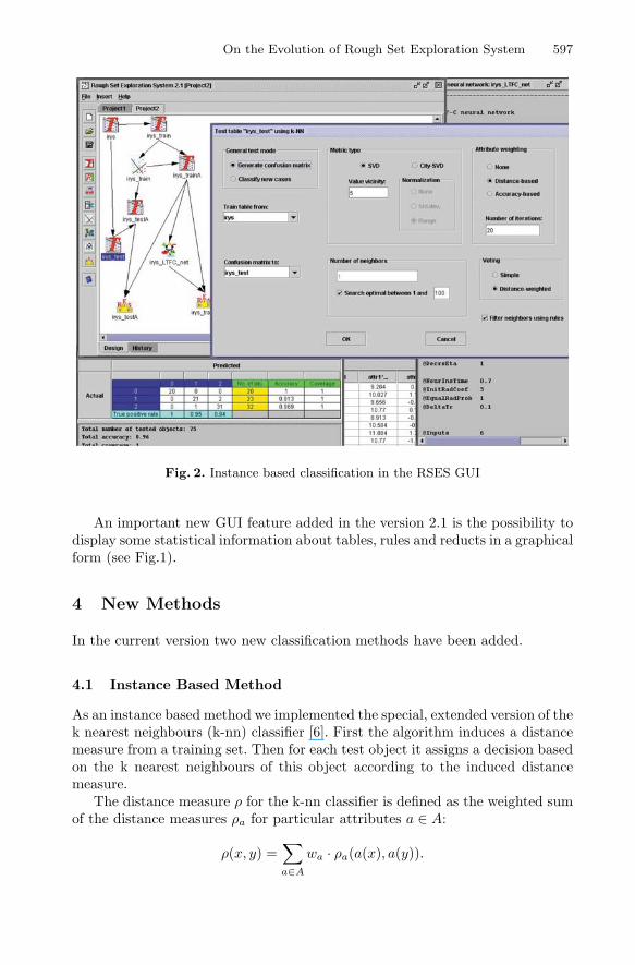
Fig. 2. Instance based classification in the RSES GUI

An important new GUI feature added in the version 2.1 is the possibility todisplay some statistical information about tables, rules and reducts in a graphicalform (see Fig.1).

4 New Methods

In the current version two new classification methods have been added.

4.1 Instance Based Method

As an instance based method we implemented the special, extended version of thek nearest neighbours (k-nn) classifier [6]. First the algorithm induces a distancemeasure from a training set. Then for each test object it assigns a decision basedon the k nearest neighbours of this object according to the induced distancemeasure.

The distance measure ρ for the k-nn classifier is defined as the weighted sumof the distance measures ρa for particular attributes a ∈ A:

ρ(x, y) =∑

a∈A

wa · ρa(a(x), a(y)).

598 Jan G. Bazan et al.

Two types of a distance measure are available to the user. The City-SVDmetric [5] combines the city-block Manhattan metric for numerical attributeswith the Simple Value Difference (SVD) metric for symbolic attributes.

The distance between two numerical values ρa(a(x), a(y)) is the difference|a(x) − a(y)| taken either as an absolute value or normalised with the rangeamax − amin or with the doubled standard deviation of the attribute a on thetraining set. The SVD distance ρa(a(x), a(y)) for a symbolic attribute a is thedifference between the decision distributions for the values a(x) and a(y) inthe whole training set. Another metric type is the SVD metric. For symbolicattributes it is defined as in the City-SVD metric and for a numerical attributea the difference between a pair of values a(x) and a(y) is defined as the differencebetween the decision distributions in the neighbourhoods of these values. Theneighbourhood of a numerical value is defined as the set of objects with similarvalues of the corresponding attribute. The number of objects considered as theneighbourhood size is the parameter to be set by a user.

A user may optionally apply one of two attribute weighting methods to im-prove the properties of an induced metric. The distance-based method is an iter-ative procedure focused on optimising the distance between the training objectscorrectly classified with the nearest neighbour in a training set. The detailed de-scription of the distance-based method is described in [15]. The accuracy-basedmethod is also an iterative procedure. At each iteration it increases the weightsof attributes with high accuracy of the 1-nn classification.

As in the typical k-nn approach a user may define the number of nearestneighbours k taken into consideration while computing a decision for a testobject. However, a user may use a system procedure to estimate the optimalnumber of neighbours on the basis of a training set. For each value k in a givenrange the procedure applies the leave-one-out k-nn test and selects the value kwith the optimal accuracy. The system uses an efficient leave-one-out test formany values of k as described in [7].

When the nearest neighbours of a given test object are found in a training setthey vote for a decision to be assigned to the test object. Two methods of nearestneighbours voting are available. In the simple voting all k nearest neighbours areequally important and for each test object the system assigns the most frequentdecision in the set of the nearest neighbours. In the distance-weighted votingeach nearest neighbour vote is weighted inversely proportional to the distancebetween a test object and the neighbour. If the option of filtering neighbourswith rules is checked by a user, the system excludes from voting all the nearestneighbours that produce a local rule inconsistent with another nearest neighbour(see [7] for details).

The k-nn classification approach is known to be computationally expensive.The crucial time-consuming task is searching for k nearest neighbours in a train-ing set. The basic approach is to scan the whole training set for each test object.To make it more efficient an advanced indexing method is used [15]. It acceler-ates searching up to several thousand times and allows to test datasets of a sizeup to several hundred thousand of objects.

On the Evolution of Rough Set Exploration System 599

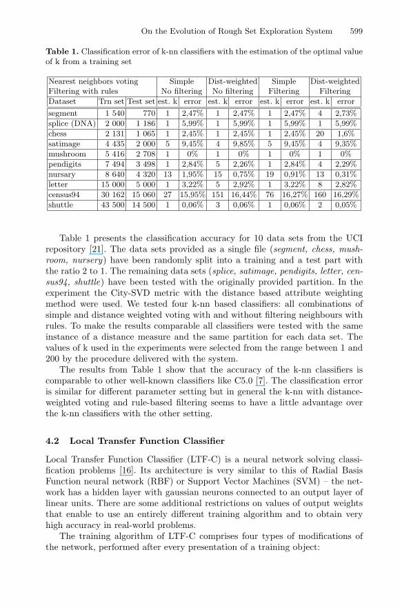
Table 1. Classification error of k-nn classifiers with the estimation of the optimal valueof k from a training set

Nearest neighbors voting Simple Dist-weighted Simple Dist-weightedFiltering with rules No filtering No filtering Filtering Filtering

Dataset Trn set Test set est. k error est. k error est. k error est. k error

segment 1 540 770 1 2,47% 1 2,47% 1 2,47% 4 2,73%

splice (DNA) 2 000 1 186 1 5,99% 1 5,99% 1 5,99% 1 5,99%

chess 2 131 1 065 1 2,45% 1 2,45% 1 2,45% 20 1,6%

satimage 4 435 2 000 5 9,45% 4 9,85% 5 9,45% 4 9,35%

mushroom 5 416 2 708 1 0% 1 0% 1 0% 1 0%

pendigits 7 494 3 498 1 2,84% 5 2,26% 1 2,84% 4 2,29%

nursary 8 640 4 320 13 1,95% 15 0,75% 19 0,91% 13 0,31%

letter 15 000 5 000 1 3,22% 5 2,92% 1 3,22% 8 2,82%

census94 30 162 15 060 27 15,95% 151 16,44% 76 16,27% 160 16,29%

shuttle 43 500 14 500 1 0,06% 3 0,06% 1 0,06% 2 0,05%

Table 1 presents the classification accuracy for 10 data sets from the UCIrepository [21]. The data sets provided as a single file (segment, chess, mush-room, nursery) have been randomly split into a training and a test part withthe ratio 2 to 1. The remaining data sets (splice, satimage, pendigits, letter, cen-sus94, shuttle) have been tested with the originally provided partition. In theexperiment the City-SVD metric with the distance based attribute weightingmethod were used. We tested four k-nn based classifiers: all combinations ofsimple and distance weighted voting with and without filtering neighbours withrules. To make the results comparable all classifiers were tested with the sameinstance of a distance measure and the same partition for each data set. Thevalues of k used in the experiments were selected from the range between 1 and200 by the procedure delivered with the system.

The results from Table 1 show that the accuracy of the k-nn classifiers iscomparable to other well-known classifiers like C5.0 [7]. The classification erroris similar for different parameter setting but in general the k-nn with distance-weighted voting and rule-based filtering seems to have a little advantage overthe k-nn classifiers with the other setting.

4.2 Local Transfer Function Classifier

Local Transfer Function Classifier (LTF-C) is a neural network solving classi-fication problems [16]. Its architecture is very similar to this of Radial BasisFunction neural network (RBF) or Support Vector Machines (SVM) – the net-work has a hidden layer with gaussian neurons connected to an output layer oflinear units. There are some additional restrictions on values of output weightsthat enable to use an entirely different training algorithm and to obtain veryhigh accuracy in real-world problems.

The training algorithm of LTF-C comprises four types of modifications ofthe network, performed after every presentation of a training object:

600 Jan G. Bazan et al.

1. changing positions (means) of gaussians,2. changing widths (deviations) of gaussians, separately for each hidden neuron

and attribute,3. insertion of new hidden neurons,4. removal of unnecessary or harmful hidden neurons.

As one can see, the network structure is dynamical. The training process startswith an empty hidden layer, adding new hidden neurons when the accuracyis insufficient and removing the units which do not positively contribute to thecalculation of correct network decisions. This feature of LTF-C enables automaticchoice of the best network size, which is much easier than setting the numberof hidden neurons manually. Moreover, this helps to avoid getting stuck in localminima during training, which is a serious problem in neural networks trainedwith gradient-descend.

LTF-C shows a very good performance in solving real-world problems. Asystem based on this network won the first prize in the EUNITE 2002 WorldCompetition “Modelling the Bank’s Client behaviour using Intelligent Technolo-gies”. The competition problem was to classify bank customers as either activeor non-active, in order to predict if they would like to leave the bank in the near-est future. The system based on LTF-C achieved 75.5% accuracy, outperformingmodels based on decision trees, Support Vector Machines, standard neural net-works and others (see [20]) .

LTF-C performs also very well in other tasks, such as handwritten digitrecognition, breast cancer diagnosis or credit risk assessment (details in [16]).

5 Perspective

The RSES toolkit will further grow as new methods and algorithms emerge.More procedures are still coming from current state-of-the-art research. Mostnotably, the work on a new version of the RSESlib library of methods is wellunder way. Also, currently available computational methods are being integratedwith DIXER - a system for distributed data processing.

The article reflects the state of software tools at the moment of writing, i.e.beginning of March 2004. For information on most recent developments visit theWeb site [18].

Acknowledgement

Many persons have contributed to the development of RSES. In the first placeProfessor Andrzej Skowron, the supervisor of all RSES efforts from the verybeginning. Development of our software was supported by grants 4T11C04024and 3T11C00226 from Polish Ministry of Scientific Research and InformationTechnology.

On the Evolution of Rough Set Exploration System 601

References

1. Bazan, J.: A Comparison of Dynamic and non-Dynamic Rough Set Methods forExtracting Laws from Decision Tables, In [13], vol. 1, pp. 321–365

2. Bazan, J.G., Nguyen, S.H, Nguyen, H.S., Synak, P., Wroblewski, J.: Rough SetAlgorithms in Classification Problem. In: Polkowski, L., Tsumoto, S., Lin, T.Y.(eds), Rough Set Methods and Applications, Physica-Verlag, Heidelberg, 2000 pp.49–88.

3. Bazan, J., Szczuka, M.,: RSES and RSESlib - A Collection of Tools for Rough SetComputations. Proc. of RSCTC’2000, LNAI 2005, Springer-Verlag, Berlin, 2001,pp. 106–113

4. Bazan, J., Szczuka, M., Wroblewski, J.: A New Version of Rough Set ExplorationSystem. Proc. of RSCTC’2002, LNAI 2475, Springer-Verlag, Berlin, 2002, pp. 397–404

5. Domingos, P.: Unifying Instance-Based and Rule-Based Induction. Machine Learn-ing, Vol. 24(2), 1996, pp. 141–168.

6. Duda, R.O., Hart, P.E.: Pattern Classification and Scene Analysis, Wiley, NewYork, 1973.

7. Gora, G., Wojna, A.G.: RIONA: a New Classification System Combining Rule In-duction and Instance-Based Learning. Fundamenta Informaticae, Vol. 51(4), 2002,pp. 369–390.

8. Grzyma�la-Busse, J.: A New Version of the Rule Induction System LERS. Funda-menta Informaticae, Vol. 31(1), 1997, pp. 27–39

9. Grzyma�la-Busse, J., Hu, M.: A Comparison of Several Approaches to Missing At-tribute Values in Data Mining. Proc. of RSCTC’2000, LNAI 2005, Springer-Verlag,Berlin, 2001, pp. 340–347

10. Nguyen Sinh Hoa, Nguyen Hung Son: Discretization Methods in Data Mining. In[13] vol.1, pp. 451-482

11. Hoa S. Nguyen, Skowron, A., Synak, P.: Discovery of Data Patterns with Applica-tions to Decomposition and Classfification Problems. In [13] vol.2, pp. 55-97.

12. Michie, D., Spiegelhalter, D.J., Taylor, C.C.: Machine Learning, Neural and Sta-tistical Classification. Ellis Horwood, London, 1994

13. Skowron A., Polkowski L.(ed.): Rough Sets in Knowledge Discovery vol. 1 and 2.Physica-Verlag, Heidelberg, 1998

14. Slezak, D., Wroblewski, J.: Classification Algorithms Based on Linear Combina-tions of Features. Proc. of PKDD’99, LNAI 1704, Springer-Verlag, Berlin, 1999,pp. 548–553.

15. Wojna, A.G.: Center-Based Indexing in Vector and Metric Spaces. FundamentaInformaticae, Vol. 56(3), 2003, pp. 285-310.

16. Wojnarski, M.: LTF-C: Architecture, Training Algorithm and Applications of NewNeural Classifier. Fundamenta Informaticae, Vol. 54(1), 2003, pp. 89–105

17. Wroblewski, J.: Covering with Reducts - A Fast Algorithm for Rule Generation.Proceeding of RSCTC’98, LNAI 1424, Springer-Verlag, Berlin, 1998, pp. 402-407

18. Bazan, J., Szczuka, M.: The RSES Homepage,http://logic.mimuw.edu.pl/∼rses

19. Ørn, A.: The ROSETTA Homepage, http://www.idi.ntnu.no/∼aleks/rosetta20. Report from EUNITE World competition in domain of Intelligent Technologies,

http://www.eunite.org/eunite/events/eunite2002/competitionreport2002.htm

21. Blake, C.L., Merz, C.J.:UCI Repository of machine learning databases. Irvine, CA:University of California, 1998, http://www.ics.uci.edu/∼mlearn