Omega-analysis and 0.999... (rough translation)

Curt Schmieden and Detlef Laugwitz developed the so-called omega-analysis (a form of differential and integral calculus with infinitely great and infinitely small numbers). This system can be considered as a precursor to the more comprehensive and abstract non-standard analysis of Abraham Robinson. In the omega-analysis, we can construct a type of decimal numbers (the parareal numbers) for which 0.999... < 1.000... .

Omega-analysis The basic ideas of omega-analysis are essentially quite simple. (For more information see [8], [14] and [16].) This system of the German mathematicians Curt Schmieden (1905-1992) and Detlef Laugwitz (1932-2000) is to be regarded as a precursor of the non-standard analysis of Abraham Robinson [13]. The mathematical relationship between omega-analysis and non-standard analysis is treated in [8]. Schmieden and Laugwitz base their system on infinite sequences of real or rational numbers that are added and multiplied component wise. These sequences they consider as omega-numbers (Ω-Zahlen). For convenience, we here work with sequences of real numbers. Sequences that have the same number for each component correspond to the ordinary real numbers. Thus, the numbers 1, 2 and √3 correspond to:

(1, 1, 1, 1, ... , 1, ...) , (2, 2, 2, 2, ... , 2, ...) & (√3, √3, √3, √3, ... , √3, ...) .

The sum and the product of the second and third sequence are:

(2+√3, 2+√3, 2+√3, 2+√3, ... , 2+√3, ...) , (2 .√3, 2 .√3, 2 .√3, 2 .√3, ... , 2 .√3, ...) .

In the same way 'copies' of all the real numbers find their place in omega-analysis. For convenience, we wil denote a sequence in which all components are equal to a real number α by α*. We will call them omega copies. With such sequences we can calculate as if they were the actual real numbers themselves.

But all omega-numbers a and b - whether they are omega-copies or not - can be written in the form:

a = (a0 , a1 , a2 , a3 , ... , an , ...) , b = (b0 , b1 , b2 , b3 , ... , bn , ...) .

In the general case we therefore have:

a + b = (a0 + b0 , a1 + b1 , a2 + b2 , a3 + b3 , ... , an + bn , ...) , a . b = ( a0 . b0 , a1 . b1 , a2 . b2 , a3 . b3 , ... , an . bn , ...) .

Further we call a equal to b (written as a = b) then and only then when an = bn for all natural numbers n (including 0).

We call a finally equal to b (written as a ≃ b) then and only then when there exists a natural number N such that an = bn for all n > N.

We call a approximately equal to b (written as a ≈ b) then and only then when for any positive real number ε (no matter how small) there is a natural number N such that │ an - bn │ < ε for all natural numbers n > N.

Whenever two omega-numbers are equal, they are also finally equal and approximately equal. And whenever two omega-numbers are finally equal, they are also approximately equal.

Commutative ring It is easy to show that the omega-numbers together with the above introduced addition + and multiplication . satisfy the following properties:

(i) For all omega-numbers a and b the sum a + b and the product a . b are also omega-numbers (so that + and . are internal operations).

(ii) For all omega-numbers a and b we have: a + b = b + a and a . b = b . a (commutativity).

(iii) For all omega-numbers a, b and c we have: a + (b + c) = (a + b) + c and a .(b . c) = (a . b) . c (associativity).

(iv) For all omega-numbers a, b and c we have: a. (b + c) = a .b + a .c (distributivity).

(v) There exists an omega-number 0 such that a + 0 = a for all omega-numbers a (existence of a zero-element).

(vi) There exists an omega-number 1 ≠ 0 such that a . 1 = a for all omega-numbers a (existence of an one-element).

(vii) For all omega-numbers a the equation a + x = 0 has an omega-number x as a solution (existence of an opposite).

The zero-element 0 and the one-element 1 are:

0 = (0, 0, 0, ... , 0, ...) , 1 = (1, 1, 1, ... , 1, ...) .

Clearly for all omega-numbers a there exists an opposite -a . To see this let us write the omega-number a as:

a = (a0 , a1 , a2 , a3 , ... , an , ...) .

Than the omega-number -a with:

-a = (-a0 , -a1 , -a2 , -a3 , ... , -an , ...) ,

clearly satisfies the equation a + -a = 0 .

We define the difference a - b of two omega-numbers a and b as: a + -b.

That the other properties are also satisfied, can easily be proven from corresponding properties of the real numbers.

A (number) system that satisfies properties (i) to (vii) in abstract algebra is called a commutative ring. Therefore our system of the omega-numbers with the indicated addition and multiplication is a commutative ring.

Ordering For convenience, we here and later write {x}k for the k-th component xk of the omega-number:

x = (x0 , x1 , x2 , x3 , ... , xn , ...) .

The ordering of the omega-numbers we define as follows.

We call a greater than b (written as a > b) then and only then when there exists a natural number N such that {a}n > {b}n for all n > N.

We call a smaller than b (written as a < b) then and only then when there exists a natural number N such that {a}n < {b}n for all n > N.

We can write the omega-numbers α* and β*, which correspond to the real numbers α and β, as the constant sequences:

α* = (α , α , α , α , ... , α , ...) , β* = (β , β , β , β , ... , β , ...) .

For which it of course holds that:

α* = β* then and only then when α = β , α* > β* then and only then when α > β , α* < β* then and only then when α < β .

Thus we see that our definition for the ordering of the omega-numbers respects the usual ordering of the real numbers.

For the omega-copies 0.999...* and 1* (of the real numbers 0.999... and 1) in particular it holds that: 0.999...* = 1*. This can be seen as follows. The equality or inequality of two omega-copies α* and β* (of the real numbers α and β) is determined by comparison of the corresponding components of α* and β*. But all components of α* are α and all components of β* are β . The equality or inequality of the two omega-copies α* and β* therefore depends on the equality or inequality of the real numbers α and β . But within the system of the real numbers it holds that 0.999... and 1 are equal. Therefore the same has to hold for 0.999...* and 1*. Only later in this article will we introduce the parareal numbers. These will be defined independently of the omega-copies. As we will then see the parareal numbers «+0.999...» and «+1.000...» are unequal.

There are omega-numbers a and b for which none of the five relations a = b, a ≃ b, a ≈ b, a > b or a < b applies. An example is:

a = (1, 0, 1, 0, 1, ... , 1, 0, ...) , b = (0, 1, 0, 1, 0, ... , 0, 1, ...) .

Because we are going to need it anyway, let us here already define the absolute value │a│ of an omega-number a . For:

a = (a0 , a1 , a2 , a3 , ... , an , ...) ,

we set:

│a│ = (│a0│, │a1│, │a2│, │a3│, ... , │an│, ...) .

Finally, let us give an example. Let:

a = (0, 1, 2, 3, 2, 1, 0, -1, -2, -3, -2, -1, 0, 1, 2, 3, 2, ...) .

Then:

-a = (0, -1, -2, -3, -2, -1, 0, 1, 2, 3, 2, 1, 0, -1, -2, -3, -2, ...) .

And also:

│a │ = │-a│ = (0, 1, 2, 3, 2, 1, 0, 1, 2, 3, 2, 1, 0, 1, 2, 3, 2, ...) .

Infinitely great and infinitely small omega-numbers The nice thing is that we can now easily imagine a sequence whose components keep on increasing. By the omega-number Ω we mean:

Ω = (0, 1, 2, 3, ... , n, ...) .

The components of this sequence Ω eventually pass by any chosen positive real number α . So:

│Ω│ > α* ,

for all positive real numbers α . Omega-numbers with this property we call infinitely great.

A precise definition runs as follows: We call an omega-number a infinitely great then and only then when for any positive real number r (no matter how great) there is a natural number N such that: │{a}n │ > r for all n > N .

We can also have infinitely small or infinitesimal omega-numbers. The following example ω is found by taking (except for the first component) the reciprocal of the components of the previous sequence:

ω = (1, 1, ½, ⅓, ... , 1/n , ...) .

The components of this sequence ω (except for the first component) keep on becoming smaller and smaller but remain positive. For any positive real number α there is indeed a point beyond which the components of the above sequence are smaller but still positive. So:

0 <│ω│ < α* ,

for all positive real numbers α . The omega-numbers with this property we call infinitely small (or infinitesimal).

A precise definition runs as follows: We call an omega-number a infinitely small or infinitesimal then and only then when for any positive real number ε (however small) there is a natural number N such that: 0 < │{a}n │ < ε for all n > N .

(Here we do not consider zero an infinitesimal. This has advantages and disadvantages. So whether we do it or not is a matter of convention.)

For ω.Ω we find:

ω.Ω = (1.0, 1.1, ½ .2, ⅓ .3, ... , 1/n . n , ...) , ω.Ω = (0, 1, 1, 1, ... , 1 , ...) .

So: ω.Ω ≠ 1 (but ω.Ω ≃ 1 ).

Division doesn't always work For all real numbers x except 0, the reciprocal number 1/x exists. To make a function q out of it of all real numbers (that is including 0) to the real numbers, we define:

q(x) = 1/x for x ≠ 0, and q(0) = 0 .

We can always apply such a trick to transform real functions that are not defined for all real numbers, into real functions that are defined for all real numbers. This has the disadvantage that the so obtained function has meaningless zero results for certain arguments. The advantage is that we do not need to worry about any possible restrictions in the domain of the real functions, when extending those real functions to functions from the omega-numbers to the omega-numbers.

Next we define the function q* from the omega-numbers to the omega-numbers as follows:

For all arguments:

x = (x0 , x1 , x2 , x3 , ... , xn , ...) ,

let:

q*(x) = ( q(x0 ), q(x1 ), q(x2 ), q(x3 ), ... , q(xn ), ...) .

Also, we call an omega-number:

a = (a0 , a1 , a2 , a3 , ... , an , ...) ,

zero-free exactly then, when none of the components a0 , a1 , a2 , a3 , ... , an , ... is equal to 0.

For all zero-free omega-numbers a we than have:

q*(a) . a = ( q(a0 ), q(a1 ), q(a2 ), q(a3 ), ... , q(an ), ...) . (a0 , a1 , a2 , a3 , ... , an , ...) , q*(a) . a = ( q(a0 ). a0 , q(a1 ).a1 , q(a2 ).a2 , q(a3 ).a3 , ... , q(an ).an , ...) , q*(a) . a = ((1/a0 ). a0 , (1/a1 ).a1 , (1/a2 ).a2 , (1/a3 ).a3 , ... , (1/an ).an , ...) , q*(a) . a = (1, 1, 1, 1, ... , 1, ...) , q*(a) . a = 1 .

For all omega-numbers α* (with α ≠ 0) in particular, we find:

q*(α*) . α* = 1 .

Therefore, when dealing with omega-numbers we can divide by α* (for α ≠ 0). Just as in the ordinary real numbers.

An omega-number a we call finally zero-free then and only then when there exists a natural number N such that none of the components aN+1 , aN+2 , aN+3 , ... , aN+n , ... is equal to 0.

An example is Ω. We find:

q*(Ω) = q*((0, 1, 2, 3, ... , n, ...)) , q*(Ω) = ( q(0), q(1), q(2), q(3), ... , q(n), ...) , q*(Ω) = (0, 1, ½, ⅓, ... , 1/n , ...) .

It is now easy to verify that:

q*(Ω) . Ω ≃ 1 .

This can be generalised. We will now prove that for all finally zero-free omega-numbers a we have:

q*(a) . a ≃ 1 .

Proof: For a we again write:

a = (a0 , a1 , a2 , a3 , ... , an , ...) ,

It then follows that:

q*(a) . a = ( q(a0 ), q(a1 ), q(a2 ), q(a3 ), ... , q(an ), ...) . (a0 , a1 , a2 , a3 , ... , an , ...) ,q*(a) . a = ( q(a0 ) . a0 , q(a1 ) . a1 , q(a2 ) . a2 , q(a3 ) . a3 , ... , q(an ) . an , ...) .

Since for all finally zero-free omega-numbers a there is a natural number N such that none of the components aN+1 , aN+2 , aN+3 , ... , aN+n , ... is equal to 0, we from the natural number N on get:

q(aN+1 ) . aN+1 = (1/aN+1 ) . aN+1 = 1 , q(aN+2 ) . aN+2 = (1/aN+2 ) . aN+2 = 1 , q(aN+3 ) . aN+3 = (1/aN+3 ) . aN+3 = 1 , ... , q(aN+n ) . aN+n = (1/aN+n ) . aN+n = 1 , ... .

The product q*(a) . a therefore is of the form:

q*(a) . a = (c0 , c1 , c2 , c3 , ... , cN , 1, 1, 1, 1, ... , 1, ...) .

Thus: q*(a) . a ≃ 1 .

Which completes the proof.

So we for all zero-free omega-numbers a have: q*(a) . a = 1 . And we for all finally zero-free omega-numbers a found: q*(a) . a ≃ 1 .

(Note that zero-free omega-numbers are always finally zero-free.)

This leads us to define the omega-reciprocal number a-1 for all zero-free and also all finally zero-free omega-numbers a as:

a-1 = q*(a) .

Furthermore we define the division a : b for all omega-numbers a and for all zero-free and finally zero-free omega-numbers b as: a : b = a . b -1 .

Hence for all omega-numbers a and all zero-free omega-numbers b we have:

(a : b) . b = (a . b-1) . b , (a : b) . b = a. (b-1. b) , (a : b) . b = a . ( q*(b) . b) , (a : b) . b = a . 1 , (a : b) . b = a .

And for all omega-numbers a and all finally zero-free omega-numbers b we get:

(a : b) . b = (a . b-1) . b , (a : b) . b = a . (b-1. b) , (a : b) . b = a . ( q*(b) . b) , (a : b) . b ≃ a . 1 , (a : b) . b ≃ a .

There are however omega-numbers a ≠ 0 that are not finally zero-free. The following sequence is an example:

(0, 1, 0, 1, ..., 0, 1, ...) .

For such omega-numbers a , in a trivial way q*(a) is still defined. But there are no omega-numbers b such that b . a = 1 or b . a ≃ 1 . Therefore we have not defined the omega-reciprocal number a-1

for omega-numbers that are not finally zero-free. Division goes very well for all zero-free omega-numbers, and we can manage (by using the final equality ≃) for all finally zero-free omega-numbers. But as we have seen, for some omega-numbers different from 0 division is not possible. To this peculiarity of omega-analysis we have to keep continuously alert.

Functions In the definition of the opposite -x of an omega-number x, of the absolute value │x│ of an omega-number x and of the image q*(x) for an omega-number x, we see a similar pattern. Always a function from the (set of) real numbers to the (set of) real numbers is transformed into a function from the (set of) omega-numbers to the (set of) omega-numbers by applying the original real function on the components of the omega-numbers that are playing the role of arguments.

Indeed, for:

x = (x0 , x1 , x2 , x3 , ... , xn , ...) ,

we have:

-x = ( -x0 , -x1 , -x2 , -x3 , ... , -xn , ...) , │x│ = ( │x0│, │x1│, │x2│, │x3│, ... , │xn│, ...) , q*(x) = ( q(x0 ), q(x1 ), q(x2 ), q(x3 ), ... , q(xn ) , ...) .

(The addition and multiplication of two omega-numbers follow the same pattern as well.)

For all functions f from the real numbers to the real numbers, we will now consider the function f* from the omega-numbers to the omega-numbers to be the function that is defined by the following scheme:

f*(x) = (f(x0 ), f(x1 ), f(x2 ), f(x3 ), ... , f(xn ), ...) .

Or more explicit:

f*((x0 , x1 , x2 , x3 , ... , xn , ...)) = (f(x0 ), f(x1 ), f(x2 ), f(x3 ), ... , f(xn ), ...) .

This function f* can be regarded as a translation to the realm of omega-numbers of the original real function f. But is f* a 'faithful version' of f ? Suppose a real function f has the real image β = f(α) for a real argument α . Then of course α* and β* are the omega-copies of α and β. Now we would like the function f* to have the image β* = f*(α*) for the argument α*. Only then can we consider f* to be a generalisation of f. Let us see if this is so.

Suppose that f is a function from the real numbers to the real numbers. Further let us assume that β = f(α) for some real numbers α and β. Then we get:

f*(α*) = f*((α , α , α , α , ... , α , ...)) , f*(α*) = (f(α), f(α), f(α), f(α), ... , f(α), ...) , f*(α*) = (β, β, β, β, ... , β, ...) , f*(α*) = β* .

So f* is indeed a generalisation of f. Therefore in practice we can often omit the asterisk. Because omega-copies α* behave just like the real numbers α , the asterisk on omega-copies can in practice also often be omitted. However, during the explanation of the theory a clear distinction between real numbers and omega-numbers and between functions f from the real numbers to the real numbers and functions f* from the omega-numbers to the omega-numbers is indispensable.

Identities Real identities are equations that are true, whatever real numbers we substitute for the individual variables. Examples are:

(a) (x + y)2 = x2 + 2 . x . y + y2, (b) exp(x + y) = exp(x) . exp(y) , (c) sin(2 . x) = 2 . sin(x) . cos(x) .

Such identities are frequently used in mathematics. We can prove that generalised forms of these identities apply to the omega-numbers. Here we will only proof the validity within omega-analysis of a generalisation of (b). Other identities can be treated in the same way. All such proofs are based on the fact that omega-numbers are - by definition - infinite sequences of real numbers.

For all omega-numbers:

x = (x0 , x1 , x2 , x3 , ... , xn , ...) , y = (y0 , y1 , y2 , y3 , ... , yn , ...) ,

we have:

exp(x0 + y0 ) = exp(x0 ) . exp(y0 ) , exp(x1 + y1 ) = exp(x1 ) . exp(y1 ) , exp(x2 + y2 ) = exp(x2 ) . exp(y2 ) , exp(x3 + y3 ) = exp(x3 ) . exp(y3 ) , ... , exp(xn + yn ) = exp(xn ) . exp(yn ) , ... .

That is:

exp({x+y}0 ) = {exp*(x)}0 . {exp*(y)}0 , exp({x+y}1 ) = {exp*(x)}1 . {exp*(y)}1 , exp({x+y}2 ) = {exp*(x)}2 . {exp*(y)}2 , exp({x+y}3 ) = {exp*(x)}3 . {exp*(y)}3 , ... , exp({x+y}n ) = {exp*(x)}n . {exp*(y)}n , ... .

Which gives:

{exp*(x+y)}0 = {(exp*(x) . exp*(y))}0 , {exp*(x+y)}1 = {(exp*(x) . exp*(y))}1 , {exp*(x+y)}2 = {(exp*(x) . exp*(y))}2 , {exp*(x+y)}3 = {(exp*(x) . exp*(y))}3 , ... , {exp*(x+y)}n = {(exp*(x) . exp*(y))}n , ... .

So:

exp*(x+y) = exp*(x) . exp*(y) .

Which completes the proof.

Limits Statements about limits in 'usual' analysis can often be translated into statements on the approximate equalness in omega-analysis. We give two important examples:

Limits of sequences

For the limit of an infinite sequence of real numbers a0 , a1 , a2 , a3 , ... , an , ... we use the following definition:

Let L be a certain real number. Then we denote the proposition that for any positive real number ε (no matter how small) there is a natural number N such that │an - L │ < ε for all n > N by:

lim an = L . n→ ∞

The above mentioned sequence of real numbers corresponds to the omega-number:

a = (a0 , a1 , a2 , a3 , ... , an , ...) .

Now it holds, as one can easily verify, that:

lim an = L ⇔ a ≈ L* . n→ ∞

Which means that the first and second statement are logically equivalent: if the first statement is true the second also has to be true, and vice versa.

Limits of functions

Let f be a function from the real numbers to the real numbers. We again consider f* to be the previously defined generalisation of f to a function from the omega-numbers to the omega-numbers. The proposition that for a real number L there exists for any positive real number ε (no matter how small) a positive real number δ such that 0 < │x - a│< δ implies │f(x) - L│< ε , we denote as:

lim f(x) = L (α) x→ a Then the above assertion (α) is logically equivalent to the undermentioned assertion (β):

For all zero-free infinitesimal omega-numbers h it holds that f*(a* + h) ≈ L* (β)

Proof: We have two things to prove. First (α) ⇒ (β) and second (β) ⇒ (α).

We start with (α) ⇒ (β). Let us therefore assume that (α) is true. And let ε0 be a positive real number. Then there is a positive real number δ such that 0 <│x - a│< δ implies │f(x) - L│< ε0 . Let δ0 be such a positive real number. Then we have:

0 < │x - a│< δ0 ⇒ │f(x) - L│< ε0 .

If h is a zero-free infinitesimal omega-number then for our δ0 there has to be a natural number N such that 0 <│{h}n│< δ0 for all natural numbers n > N . Let N0 be such a number. Then it follows that:

n > N0 ⇒ 0 <│{h}n │< δ0 ,

n > N0 ⇒ 0 <│(a + {h}n ) - a│< δ0 .

And consequently we get:

n > N0 ⇒ 0 <│(a + {h}n ) - a│< δ0 ⇒ │f(a + {h}n ) - L│< ε0 ,

n > N0 ⇒ │f(a + {h}n ) - L│< ε0 , n > N0 ⇒ │f({a*}n + {h}n ) - {L*}n │< ε0 ,

n > N0 ⇒ │f({a* + h}n ) - {L*}n │< ε0 , n > N0 ⇒ │{f*(a* + h)}n - {L*}n │< ε0 .

For ε0 we only assumed it to be is a positive real number. And for h we only assumed that it is a zero-free infinitesimal omega-number. So there are for all positive real numbers ε0 and all zero-free infinitesimal omega-numbers h corresponding N0 such that:

n > N0 ⇒ │{f*(a* + h)}n - {L*}n │< ε0 .

Thus for all zero-free infinitesimal omega-numbers h it holds that:

f*(a* + h) ≈ L* .

Wherewith it is proved that from:

lim f(x) = L ......................................................................................................... (α) , x→ a it follows that:

f*(a* + h) ≈ L*, for all zero-free infinitesimal omega-numbers h ...................... (β) .

Next we prove that (β) ⇒ (α). Thus we now assume that (β) is true. In this case, it holds for each zero-free infinitesimal omega-number h that:

f*(a* + h) ≈ L* .

Now let g be such a zero-free infinitesimal omega-number. For convenience, we will write:

g = (g0 , g1 , g2 , g3 , ... , gn , ...) .

Then there is for every positive real number ε a natural number N such that:

│{f*(a* + g)}n - {L*}n │< ε for all natural numbers n > N .

The expression U = │{f*(a* + g)}n - {L*}n │ from the above we can rewrite as:

U = │{f*(a* + g)}n - {L*}n │, U = │f({a* + g}n ) - L│, U = │f({a*}n + {g}n ) - L│, U = │f(a + gn ) - L│.

So for any positive real number ε there is a natural number N such that:

│f(a + gn ) - L│< ε for all natural numbers n > N .

And hence:

lim f(a + gn ) = L . n→ ∞ Because for our particular g we only assumed it to be a zero-free infinitesimal omega-number, the above follows for all such zero-free infinitesimal omega-numbers. Therefore we may in the undermentioned general formulation again use h. For convenience, we write:

h = (h0 , h1 , h2 , h3 , ... , hn , ...) .

Thus we find:

lim f(a + hn ) = L , for all zero-free infinitesimal omega-numbers h ....................... (γ) n→ ∞ So we have proven that: (β) ⇒ (γ).

Now suppose that (α) would not hold. Then:

lim f(x) = L , x→ a would not be true. Thus there should have to be at least one positive real number ε for which there is no positive real number δ such that 0 < │x - a│< δ implies │f(x) - L│< ε . Let ε0 be such a number. Then for ε0 there is no positive real number δ such that from 0 < │x - a│< δ it follows that │f(x) - L│< ε0 . Thus whatever positive real number δ we choose, there are always values of x that satisfy 0 < │x - a│< δ but for which │ f(x) - L │ ≥ ε0 . We now choose for all natural

numbers 0, 1, 2, 3, ..., n, ... for δ the positive real numbers δn = 10-n. Then there are values for x called: x0 , x1 , x2 , x3 , ... such that:

0 < │x0 - a│ < δ0 = 1 & │f(x0 ) - L│ ≥ ε0 , 0 < │x1 - a│ < δ1 = 1/10 & │f(x1 ) - L│ ≥ ε0 , 0 < │x2 - a│ < δ2 = 1/100 & │f(x2 ) - L│ ≥ ε0 , 0 < │x3 - a│ < δ3 = 1/1000 & │f(x3 ) - L│ ≥ ε0 , ... , 0 < │xn - a│ < δn = 10 -n & │f(xn ) - L│ ≥ ε0 ,

... .

We now form the omega-number y , with yn = xn - a . Thus we get:

y = (x0 - a , x1 - a , x2 - a , x3 - a , ... , xn - a , ...) .

We can easily verify that y is a zero-free infinitesimal omega-number. And we also see that:

│f(a + y0 ) - L│ ≥ ε0 , │f(a + y1 ) - L│ ≥ ε0 , │f(a + y2 ) - L│ ≥ ε0 , │f(a + y3 ) - L│ ≥ ε0 , ... , │f(a + yn ) - L│ ≥ ε0 , ... .

Thus it does not now hold that:

lim f(a + yn ) = L , n→ ∞ for the zero-free infinitesimal omega-number y.

This result however is in contradiction with (γ). Thus we have found that from the assumption that (α) is not true (written as ¬(α)) it follows that (γ) is not true (written as ¬(γ)). Symbolically:

¬(α) ⇒ ¬(γ) .

We already proved that: (β) ⇒ (γ). Further: in case that (β) is true, it cannot happen that (α) is false, because then (γ) would have to be both true and false. Consequently: in case that (β) is true, (α) also has to be true. That is:

(β) ⇒ (α) .

This completes the proof.

The above allows us to convert a number of basic rules for limits in the usual type of analysis into elementary rules for the 'approximate equalness' in omega-analysis.

Infinite series In the usual type of analysis, the sum S of an infinite series:

a0 + a1 + a2 + a3 + ... + an + ... ,

is defined as the limit of the sequence of partial sums: 0 S0 = ∑ ai = a0 ,

i = 0

1 S1 = ∑ ai = a0 + a1 ,

i = 0 2 S2 = ∑ ai = a0 + a1 + a2 ,

i = 0 3 S3 = ∑ ai = a0 + a1 + a2 + a3 ,

i = 0 ... , n Sn = ∑ ai = a0 + a1 + a2 + a3 + ... + an ,

i = 0 ... . n That is: S = lim Sn = lim ∑ ai .

n → ∞ n → ∞ i = 0 Because the above limit does not in all cases exist, the sum of an infinite series is not always defined.

The connection of all this with the omega-analysis can be established as follows. Because for every infinite series of real numbers:

a0 + a1 + a2 + a3 + ... + an + ... ,

all partial sums S0 , S1 , S2 , S3 , ... , Sn , ... exist and moreover are real numbers themselves, the infinite sequence of these partial sums defines the omega-number S' with:

S' = (S0 , S1 , S2 , S3 , ... , Sn , ...) .

Previously, we found the undermentioned relationship between the limit of an infinite sequence of real numbers and the approximate equalness of the omega-numbers therewith related:

lim bn = L ⇔ b ≈ L* , n→ ∞ where: b = (b0 , b1 , b2 , b3 , ... , bn , ...) .

(To avoid confusion with the terms of the earlier mentioned infinite series, we have here used b's instead of a's.)

Applied to our infinite series we get:

lim Sn = L ⇔ S' ≈ L* . n→ ∞ Another approach generalises the partial sum Sn so that it can also be determined for infinitely great natural omega-numbers n. This however requires us to know which omega-numbers may be

considered as being natural omega-numbers. We define:

Only those omega-numbers will be called natural omega-numbers of which all components are natural numbers.

Now let S(x) = Sx for all natural real numbers x, and S(x) = 0 for all non-natural real numbers x . Then S(x) is a function from the real numbers to the real numbers. We already explained how to generalise functions from the real numbers to the real numbers to functions from the omega-numbers to the omega-numbers. So we can also generalise our real function S(x) to a function S*(x) from the omega-numbers to the omega-numbers. Now it so happens that we are only interested in those images S*(x) for which x is a natural omega-number. For such x we will write S*(x) as S*x . By using this generalised partial sum S*x , we can now calculate partial sums for infinitely great indices.

To give an example, for n = Ω we find:

S*Ω = (S0 , S1 , S2 , S3 , ... , Sn , ...) = S'.

Or written differently (where we have omitted the asterisk): Ω Σ ai = (S0 , S1 , S2 , S3 , ... , Sn , ...) = S'. i = 0 Every infinite series of real numbers (whether or not it has a limit in the usual sense) can thus in principle be calculates by the methods of omega-analysis. The result wil always be an omega-number.

Even 'foolish' series such as:

1 + -1 + 1 + -1 + 1 + -1 + ... , 1 + 2 + 3 + 4 + 5 + 6 + 7 + ... , 3 + 1.10 1 + 4.10 2 + 1.10 3 + 5.10 4 + 9.10 5 + ... ,

sum to omega-numbers. The last series is a kind of revolved pi. So as we see from this example, by using omega-analysis it is also possible to introduce infinitely great 'decimal numbers' with infinitely many digits to the left of the decimal point. (I do not here mean the 10-adic numbers.) Even numbers with infinitely many digits both left and right of the decimal point are possible. For instance:

- ... 9 ... 9999.343434343434343434343434 ... 34 ... .

In such cases we may use the sequence of partial sums:

S0 = ± (a0 )

S1 = ± (a1 .10 + a0 + a -1 .10-1 )

S2 = ± (a2 .102 + a1 .10 + a0 + a -1 .10-1 + a -2 .10-2 )

S3 = ± (a3 .103 + a2 .102 + a1 .10 + a0 + a -1 .10-1 + a -2 .10-2 + a -3 .10-3 ) ... Sn = ± (an .10n + ... + a3 .103 + a2 .102 + a1 .10 + a0 + a -1 .10-1 + a -2 .10-2 + a -3 .10-3 ... + a -n .10-n ) ... (+ for positive and - for negative numbers)

In my younger years, I for a long time searched for a foundation of such 'numbers'. Well - here it is! Later I discovered that the Usenet celebrity Archimedes Plutonium also considered such 'doubly infinites' (see [11] and [12]). A more serious approach is that of Frank C. DeSua. Double-sided infinite decimal expressions that at their left side ultimately become periodical he calls double decimals. DeSua has invented an interpretation under which they actually represent real numbers [2]. The problem however with all such creations is not their logical possibility (with the concepts and techniques of modern mathematics the most strange mathematical objects can be created), but whether they lead to any interesting mathematics. A difficult point ...

Differential quotient and derived function Let f be a function from the real numbers to the real numbers. Then we define the differential quotient (df*/dx)(x) of f* for the argument x and the zero-free infinitesimal dx as:

(df*/dx)(x) = (f*(x+dx) - f*(x)) . (dx)-1 .

It is clear that this differential quotient always exists.

The derivative function f ' of the function f from the real numbers to the real numbers does not always exist. Within the usual type of analysis, for every real argument a for which the limit exists the derivative function f ' is defined as:

f '(a) = lim (f(a+h) - f(a)) . h-1 . h → 0 Now we can prove that:

f '(a) = L ⇔ [(df*/dx)(a*) ≈ L*, for all zero-free infinitesimal omega-numbers dx] .

Proof: For convenience, we use some abbreviations. We denote the statement that f '(a) = L (for some real numbers a and L) by (ζ). The statement that (df*/dx)(a*) ≈ L* for all zero-free infinitesimal omega-numbers dx, we write as (η). We therefore have to prove that: (ζ) ⇔ (η). This proof will be split into two parts. First (ζ) ⇒ (η), and second (η) ⇒ (ζ).

We start with (ζ) ⇒ (η). Let us assume that (ζ) is true. That is f '(a) = L for certain real numbers a and L. Then for every positive real number ε (no matter how small) there has to exist a positive real number δ such that from 0 <│h│< δ it follows that │(f(a+h) - f(a)).h-1 - L│< ε . Now let ε0 be a positive real number. Then there has to be a positive real number δ (call one such a number δ0 ) such that:

0 < │h│< δ0 ⇒ │(f(a +h) - f(a)) . h-1 - L│< ε0 .

Let further dx be a zero-free infinitesimal omega-number. Then there is for every positive real number θ (no matter how small) a natural number N such that: 0 <│{dx}n│< θ for all n > N. Therefore we can also find a natural number N0 such that:

n > N0 ⇒ 0 < │{dx}n│ < δ0 .

Thus it holds that:

n > N0 ⇒ 0 < │{dx}n│ < δ0 ⇒ │(f(a + {dx}n ) - f(a)).({dx}n )-1 - L│< ε0 ,

n > N0 ⇒ │(f(a + {dx}n ) - f(a)).({dx}n )-1 - L│< ε0 ,

n > N0 ⇒ │(f({a*}n + {dx}n ) - f({a*}n )).({dx}n )-1 - L│< ε0 ,

n > N0 ⇒ │(f({a* + dx}n ) - f({a*}n )).({dx}n )-1 - L│< ε0 ,

n > N0 ⇒ │({f*(a* + dx)}n - {f*(a*)}n ).({dx}n )-1 - L│< ε0 ,

n > N0 ⇒ │({f*(a* + dx)}n - {f*(a*)}n ). q ({dx}n ) - L│< ε0 , n > N0 ⇒ │{f*(a* + dx) - f*(a*)}n .{ q*(dx)}n - L │< ε0 ,

n > N0 ⇒ │{f*(a* + dx) - f*(a*)}n .{(dx)-1}n - L │< ε0 ,

n > N0 ⇒ │{(f*(a* + dx) - f*(a*)) . (dx)-1}n - {L*}n │< ε0 .

For ε0 we only assumed that it is a positive real number. Thus the result found above holds generally. That is, for any positive real number ε there is a natural number N such that:

n > N ⇒ │{(f*(a* + dx) - f*(a*)) . (dx)-1}n - {L*}n │< ε .

And consequently:

(f*(a* + dx) - f*(a*)) . (dx) -1 ≈ L* , (df*/dx)(a*) ≈ L* .

For dx we only assumed that it is a zero-free infinitesimal omega-number. Thus for all real numbers a and L satisfying f '(a) = L it holds that:

(df*/dx)(a*) ≈ L*, for all zero-free infinitesimal omega-numbers dx .

Wherewith (ζ) ⇒ (η) is proven.

Next we prove (η) ⇒ (ζ). Thus we now assume that (η) is true. In this case, for some real numbers a and L and for all zero-free infinitesimal omega-numbers dx it holds that:

(df*/dx)(a*) ≈ L*.

Let us now define the function ga from the real numbers to the real numbers. For each function f from the real numbers to the real numbers and for all real numbers a we let:

ga (h) = (f(a+h) - f(a)) . h-1 for h ≠ 0, and ga (0) = 0 .

Then, for all zero-free omega-numbers dx and all natural numbers n (including 0), we get:

{ga*(dx)}n = ga ({dx}n ) ,

{ga*(dx)}n = (f(a + {dx}n ) - f(a)) . ({dx}n )-1 ,

{ga*(dx)}n = (f({a*}n + {dx}n ) - f({a*}n )) . ({dx}n )-1 ,

{ga*(dx)}n = (f({a* + dx}n ) - f({a*}n )) . ({dx}n )-1 ,

{ga*(dx)}n = ({f*(a* + dx)}n - {f*(a*)}n ) . ({dx}n )-1 ,

{ga*(dx)}n = ({f*(a* + dx)}n + -{f*(a*)}n ) . ({dx}n )-1 ,

{ga*(dx)}n = ({f*(a* + dx)}n + {-(f*(a*))}n ) . ({dx}n )-1 ,

{ga*(dx)}n = {f*(a* + dx) + -(f*(a*))}n . ({dx}n ) -1 ,

{ga*(dx)}n = {f*(a* + dx) - f*(a*)}n . ({dx}n )-1 , {ga*(dx)}n = {f*(a* + dx) - f*(a*)}n . q({dx}n ) , {ga*(dx)}n = {f*(a* + dx) - f*(a*)}n .{ q*(dx)}n ,

{ga*(dx)}n = {f*(a* + dx) - f*(a*)}n .{(dx)-1}n ,

{ga*(dx)}n = {(f*(a* + dx) - f*(a*)) . (dx)-1}n .

So:

ga*(dx) = (f*(a* + dx) - f*(a*)) . (dx)-1 .

That is, for all zero-free infinitesimal omega-numbers dx, we have:

ga*(dx) = (df*/dx)(a*) .

Therefore (assuming that (η) is true) for all zero-free infinitesimal omega-numbers dx it holds that:

ga*(dx) ≈ L*.

Here we can use the previously found result on the limits of functions. This gets us:

lim ga(h) = L . h→ 0 Substituting ga gives:

lim ((f(a+h) - f(a)) . h-1) = L. h→ 0

That is:

f '(a) = L.

Wherewith (η) ⇒ (ζ) also is proven.

And there's much more... It would be nice to also here cover other basic concepts of analysis such as the continuity of functions and the operation of integration. And we could even go much further. Detlef Laugwitz has shown how by using omega-analysis the so-called generalised functions - such as the Dirac delta-function - can also be introduced (see [6]). Even a version of the operational calculus of the Polish mathematician Jan Mikusiński (1913 - 1987) can be developed by the use of omega-analysis (see [7]). Although very interesting, all this would lead us too far astray. Moreover, it deflects from the purpose of this article: the construction of an alternative number system in which 1 ≠ 0.999...9... .

Childhood memoryDetlef Laugwitz, one of the founders of omega-analysis, notes the following about his first acquaintance with infinitesimals:

"Other reminiscences go back to my childhood. I suppose I was a boy of about 12 when our mathematics teacher asked what a circle and its tangent have in common. My spontaneous answer was: Nothing. A point was "nothing" to me. If they had anything in common, this something must have some extension, very small, practically invisible of course. My teacher, whom I remember quite well, did not subdue this curious aberration of my mind. Moreover, at about the same time he even encouraged another glimpse of the infinitesimal which must have occurred to everybody who does not simply believe in textbooks: Is 0.9... really equal to 1? Shouldn't it be less than 1? Actually, the usual "proofs" at that level are far from convincing, and objections like those ascribed to Zeno of Elea should come to the mind of everyone who is not infected by the 19th century dogma of the real numbers." (See [9] p. 2.)

A promising note. Detlef D. Spalt, a student of Laugwitz, gives a further elaboration ([15] pp. 352-370). Our explorations are in a similar vein.

Parareal numbers The decimal notation of the real numbers has, within the usual theory of the real numbers, a precise meaning which leads to 1 = 0.999...9... . Our aim, however, is to find an interpretation in which this equality does not hold. Now we cannot have both 1 = 0.999...9... and 1 ≠ 0.999...9... . Therefore we must make it clear that our alternative interpretation of 0.999...9... differs from the usual one. This can be done in many ways. I have chosen to write our alternative decimal numbers, which I will call parareal numbers, as «t cm ... c3c2c1c0.c-1c-2c-3 ... c-n ...». I use French quotation marks. Thus it becomes clear, even in the notation, that these are not the usual decimal numbers. Positive and negative numbers will be indicted by taking for t the symbol '+' or '-' respectively. We will regard an expression of the form:

«t cm ... c3c2c1c0.c-1c-2c-3 ... c-n ...» ,

as a designation of the corresponding infinite sequence of real numbers:

(φ0 , φ1 , φ2 , φ3 , ... , φn , ...) .

Where:

φ0 = sg(t).(cm .10m + ... + c3 .103 + c2 .102 + c1 .10 + c0 )

φ1 = sg(t).(cm .10m + ... + c3 .103 + c2 .102 + c1 .10 + c0 + c -1 .10-1 )

φ2 = sg(t).(cm .10m + ... + c3 .103 + c2 .102 + c1 .10 + c0 + c -1 .10-1 + c-2 .10-2 )

φ3 = sg(t).(cm .10m + ... + c3 .103 + c2 .102 + c1 .10 + c0 + c -1 .10-1 + c-2 .10-2 + c-3 .10-3 ) ... φn = sg(t).(cm .10m + ... + c3 .103 + c2 .102 + c1 .10 + c0 + c -1 .10-1 + c-2 .10-2 + c-3 .10-3 + ... + c-n .10-n ) ...

In which: sg(+) = 1 and sg(-) = -1 . And where the digits cm , ... , c3 , c2 , c1 , c0 , c-1 , c-2 , c-3 , ... , c-n , ... are to be chosen from 0, 1, 2, 3, 4, 5, 6, 7, 8 and 9.

So that we have:

φ0 = sg(t) . cm ... c3c2c1c0 φ1 = sg(t) . cm ... c3c2c1c0.c-1 φ2 = sg(t) . cm ... c3c2c1c0.c-1c-2 φ3 = sg(t) . cm ... c3c2c1c0.c-1c-2c-3 ... φn = sg(t) . cm ... c3c2c1c0.c-1c-2c-3 ... c-n ...

Any expression of the form «t cm ... c3c2c1c0.c-1c-2c-3 ... c-n ...» thus designates the corresponding sequence of real numbers. Such infinite sequences of real numbers are - by definition - omega-numbers. With the parareal numbers we can therefore calculate in the way already explained for omega-numbers. In addition to all parareal numbers also all omega-copies a* of real numbers a belong to the omega-numbers. The parareal numbers therefore are as it were standing besides the (copies of the) real numbers.

We can also look at the φk (neglecting the sign) as partial sums of the series:

(cm .10m + ... + c3 .103 + c2 .102 + c1 .101 + c0 .100 ) + c-1 . 10-1 + c-2 .10-2 + c-3 .10-3 + ... + c-n .10-n + ... .

That is: n

φn = sg(t) . Σ c-i .10-i .

i =-m Because:

Ω = (0, 1, 2, 3, ... , n, ...) & «t cm ... c3c2c1c0.c-1c-2c-3 ... c-n ...» = (φ0 , φ1 , φ2 , φ3 , ... , φn , ...) ,

we now also have: Ω

«t cm ... c3c2c1c0.c-1c-2c-3 ... c-n ...» = (sg(t))* . Σ c-i .10-i .

i = -m Here the sum is generalised in our usual way to a function from the (natural) omega-numbers to the omega-numbers.

In the special cases of «+1.000...» and «+0.999...» we get the sequences:

«+1.000...0...» = (1, 1.0, 1.00, 1.000, ... , 1.000...0 (with n zeros) , ...) , «+0.999...9...» = (0, 0.9, 0.99, 0.999, ... , 0.999...9 (with n nines) , ...) .

We immediately see that:

«+0.999...9...» < «+1.000...0...» .

And further it is clear that:

«+1.000...0...» - «+0.999...9...» = (1, 0.1, 0.01, 0.001, 0.0001, 0.00001, 0.000001, ...) .

The above difference, called by Professor Edgar E. Escultura the dark number d* (see [3]), is to be regarded as infinitesimal, just like our earlier example ω. We will take over Escultura's notation. But to indicate that it is not the omega-copy of a real number d, we will write d * in italics (as d*). We thus find:

«+1.000...0...» = «+0.999...9...» + d* .

Proof that 0.999 ... = 1 fails A familiar argument why the numbers 1 and 0.999 ... should be equal, goes like this:

9 . 0.999... = (10 - 1) . 0.999... , 9 . 0.999... = 10 . 0.999... - 1 . 0.999... , 9 . 0.999... = 9.999... - 0.999... , 9 . 0.999... = 9 , 0.999... = 9/9 ,0.999... = 1 .

If the parareal numbers form a consistent system, the above derivation as tailored to the real numbers has to be impossible for the parareal numbers. Let's see:

«+9.000...0...» . «+0.999...9...» = «+9.000...0...» . «+0.999...9...» , «+9.000...0...» . «+0.999...9...» = (9, 9, 9, 9, ...) . «+0.999...9...» , «+9.000...0...» . «+0.999...9...» = (10-1, 10-1, 10-1, 10-1, ...) . «+0.999...9...» , «+9.000...0...» . «+0.999...9...» = ((10, 10, 10, 10, ...) - (1, 1, 1, 1, ...)) . «+0.999...9...» , «+9.000...0...» . «+0.999...9...» = («+10.000...0...» - «+1.000...0...») . «+0.999...9...» .

Until this point every thing works out the same for the parareal numbers as for the real numbers. For convenience, we below denote («+10.000...0...» - «+1.000...0...») . «+0.999...9...» by ψ. So we get:

«+9.000...0...» . «+0.999...9...» = ψ .

Working out ψ gives:

ψ = («+10.000...0...» - «+1.000...0...») . «+0.999...9...» , ψ = («+10.000...0...» + -«+1.000...0...») . «+0.999...9...» , ψ = («+10.000...0...» + «-1.000...0...») . «+0.999...9...» , ψ = «+0.999...9...».(«+10.000...0...» + «-1.000...0...») , ψ = «+0.999...9...».«+10.000...0...» + «+0.999...9...».«-1.000...0...» , ψ = (0, 0.9, 0.99, 0.999, ...).(10, 10, 10, 10, ...) + (0, 0.9, 0.99, 0.999, ...).(-1, -1, -1, -1, ...) , ψ = (0, 9, 9.9, 9.99, ...) + (0, -0.9, -0.99, -0.999, ...) , ψ = ((9, 9.9, 9.99, 9.999, ...) + (-9, -0.9, -0.09, -0.009, ...)) + (0, -0.9, -0.99, -0.999, ...) , ψ = ((-9, -0.9, -0.09, -0.009, ...) + (9, 9.9, 9.99, 9.999, ...)) + (0, -0.9, -0.99, -0.999, ...) , ψ = (-9, -0.9, -0.09, -0.009, ...) + ((9, 9.9, 9.99, 9.999, ...) + (0, -0.9, -0.99, -0.999, ...)) , ψ = (-9, -0.9, -0.09, -0.009, ...) + (9, 9, 9, 9, ...) , ψ = (9, 9, 9, 9, ...) + (-9, -0.9, -0.09, -0.009, ...) , ψ = (9, 9, 9, 9, ...).(1, 1, 1, 1, ...) + (9, 9, 9, 9, ...).(-1, -0.1, -0.01, -0.001, ...) , ψ = (9, 9, 9, 9, ...).((1, 1, 1, 1, ...) + (-1, -0.1, -0.01, -0.001, ...)) , ψ = (9, 9, 9, 9, ...).((1, 1, 1, 1, ...) + -(1, 0.1, 0.01, 0.001, ...)) , ψ = (9, 9, 9, 9, ...).((1, 1, 1, 1, ...) - (1, 0.1, 0.01, 0.001, ...)) , ψ = «+9.000...0...» . («+1.000...0...» - d* ) .

This result we substitute back in «+9.000...0...» . «+0.999...9...» = ψ. So:

«+9.000...0...» . «+0.999...9...» = «+9.000...0...» . («+1.000...0...» - d* ) .

This already looks very different from the real case. It is however exactly what, given the definition of d*, was to be expected. Because «+9.000...0...» = (9, 9, 9, 9, ...) we may now, as in the real case, divide out «+9.000...0...» on both sides. This gives:

«+0.999...9...» = «+1.000...0...» - d* .

From which we see that everything develops neatly as we want it for the parareal numbers to happen; and that the difference of «+0.999...9...» and «+1.000...0...» is indeed infinitesimal.

No closed system When we add or multiply two real numbers α and β the sum α + β and the product α . β are again real numbers. This fact that the addition and multiplication of real numbers are internal operations, is an important feature of the real numbers. For the omega-copies α* and β* of the real numbers α and β the same holds true. That is, for all real numbers α and β we have:

α* + β* = (α + β)* , α* . β* = (α . β)* .

Thus the omega-copies of the real numbers with respect to addition and multiplication also form a closed system, within the omega-numbers.

For the parareal numbers this no longer holds. Indeed:

«+1.000...0...» + «-0.999...9...» = (1, 1/10, 1/100, 1/1000, ... , 1/10n , ...) .

This outcome (that is d*) is a strictly decreasing infinite sequence of positive real numbers. This omega-number cannot, on account of the definition of the parareal numbers, itself be a parareal number. Thus the parareal numbers, with respect to addition, do not form a closed system.

For the sequel it is useful to introduce some concise arithmetical notations. Let b be a real number, k a positive natural number and a an omega-number with:

a = (a0 , a1 , a2 , a3 , ... , an , ...) .

Then we define the hybrid addition, subtraction, multiplication and exponentiation as:

a + b = (a0 + b, a1 + b, a2 + b, a3 + b, ... , an + b, ...) , a - b = (a0 - b, a1 - b, a2 - b, a3 - b, ... , an - b, ...) , b . a = (b . a0 , b . a1 , b . a2 , b . a3 , ... , b . an , ...) ,

a k = ((a0 )k , (a1 )k , (a2 )k , (a3 )k , ... , (an )k , ...) ,

k a = (k^(a0 ) , k^(a1 ) , k^(a2 ) , k^(a3 ) , ... , k^(an ) , ...) .

It is clear that:

a + b = a + b* (where the first sum is hybrid and the second a sum of omega-numbers) ,a - b = a - b* (where the first difference is hybrid and the second a difference of omega-numbers) ,

b . a = b*. a (where the first product is hybrid and the second a product of omega-numbers) ,a k = a . a . a . a . ... . a (with k factors of a) .

A decimal notation for d* What would an extended decimal notation for d* look like? We have:

d* = (1, 0.1, 0.01, 0.001, 0.0001, 0.00001, 0.000001, ...) , d* = (1, 1/10, 1/100, 1/1000, ... , 1/10n , ...) , d* = (100 , 10-1 , 10-2 , 10-3 , ... , 10-n , ...) , d* = 10-Ω .

It therefore seems plausible to write d* as:

d* = +0.000...0...;...0...0001000...0... . -Ω The '1' here stands on the place indexed with -Ω.

That all -nΩ should be considered as different omega-numbers, we can see as follows. For all natural numbers n we have:

(-nΩ) - (-(n+1)Ω) = -nΩ + -(-(n+1)Ω) , (-nΩ) - (-(n+1)Ω) = -nΩ + (n+1)Ω) , (-nΩ) - (-(n+1)Ω) = -nΩ + (nΩ + Ω) , (-nΩ) - (-(n+1)Ω) = (-nΩ + nΩ) + Ω , (-nΩ) - (-(n+1)Ω) = 0* + Ω , (-nΩ) - (-(n+1)Ω) = Ω .

Thus we see that -nΩ > -(n+1)Ω , for all natural numbers n . That is:

0 > -Ω > -2Ω > -3Ω > ... > -nΩ > -(n+1)Ω > ... .

Further, for all natural numbers a, b, n and i it holds that:

{-nΩ - a}i - {-(n+1)Ω + b}i = (-n.i - a) - (-(n+1).i + b) , {-nΩ - a}i - {-(n+1)Ω + b}i = -n.i - a + (n+1).i - b , {-nΩ - a}i - {-(n+1)Ω + b}i = i - (a + b) .

So:

(-nΩ - a) > (-(n+1)Ω + b) .

Therefore after the usual sequence of indices 0, -1, -2, -3, ... , -n, ... we can, for our extended decimal notation, in principle also make use the (multiply) infinite sequence of indices:

... , -Ω+3, -Ω+2, -Ω+1, -Ω, -Ω-1, -Ω-2, -Ω-3, ... ;

... , -2Ω+3, -2Ω+2, -2Ω+1, -2Ω, -2Ω-1, -2Ω-2, -2Ω-3, ... ;

... , -3Ω+3, -3Ω+2, -3Ω+1, -3Ω, -3Ω-1, -3Ω-2, -3Ω-3, ... ;

... ,

... , -nΩ+3, -nΩ+2, -nΩ+1, -nΩ, -nΩ-1, -nΩ-2, -nΩ-3, ... ;

... .

(By using powers of Ω this may, if necessary, be yet further expanded. Then we can raise Ω to the Ω-th power. And so on. And so on.)

Because:

d* = (100 , 10-1 , 10-2 , 10-3 , ... , 10-n , ...) ,

we get:

(d*)m = ((100 )m , (10-1 )m , (10-2 )m , (10-3 )m , ... , (10-n )m , ...) , (d*)m = (100.m , 10-1.m , 10-2.m , 10-3.m , ... , 10-nm , ...) , (d*)m = (10-m.0 , 10-m.1 , 10-m.2 , 10-m.3 , ... , 10-mn , ...) , (d*)m = 10^(-m.0, -m.1, -m.2, -m.3, ... , -m.n, ...) , (d*)m = 10^(-m.(0, 1, 2, 3, ... , n, ...)) , (d*)m = 10^(-m.Ω) , (d*)m = 10-mΩ .

It is therefore plausible to write (d*)m for positive natural numbers m as:

(d*)m = +0.000...0...;...0...0001000...0... . -mΩ

Looking for a more general representation The extended decimal notations for d* and (d*)m are interesting. Is it perhaps possible to write many more parareal numbers and other omega-numbers derived therefrom, in a similar way? We will try some examples. But first for clarity, I wish to point out that this section is of a purely heuristic nature. Nothing gets proofed here! Only afterwards, with the introduction of the 'omega-decimal development', will the results here obtained get a solid mathematical basis.

We have already seen that we may write: Ω

«t cm ... c3c2c1c0.c-1c-2c-3 ... c-n ...» = (sg(t))* . Σ c-i .10-i .

i = -m Or with the hybrid multiplication: Ω

«t cm ... c3c2c1c0.c-1c-2c-3 ... c-n ...» = sg(t) . Σ c-i .10-i .

i = -m Therefore it would be nice if we had:

«t cm...c3c2c1c0.c-1c-2c-3...c-n...» = t cm...c3c2c1c0.c-1c-2c-3...c-n...;...d-Ω+n...d-Ω+3d-Ω+2d-Ω+1d-Ω000...0... .

Let us take a simple example. For «+0.999...9...» it is plausible to write:

«+0.999...9...» = +0.999...9...;...9...9999000...0... . -Ω Similarly for «+0.333...3...» we would then write:

«+0.333...3...» = +0.333...3...;...3...3333000...0... . -Ω But what should u = «+5.000...0...».«+0.333...3...» be? Let's work it out:

{u}n = {«+5.000...0...» . «+0.333...3...»}n ,{u}n = {«+5.000...0...»}n .{«+0.333...3...»}n , {u}n = (5.000...0 (with n zeros)).(0.333...3 (with n threes)) , {u}n = 5.(⅓ . 0.999...9 (with n nines)) ,

{u}n = 5 . ⅓ . (1 - 10-n ) ,

{u}n = (1.666...6...).(1 - 10-n ) ,

{u}n = (1.666...6...) - (1.666...6...).10-n .

Thus:

{u}0 = (1.666...6...) - (1.666...6...).10-0 = (1.6666666666...) - (1.6666666666...) = 0 ,

{u}1 = (1.666...6...) - (1.666...6...).10-1 = (1.6666666666...) - (0.1666666666...) = 1.5 ,

{u}2 = (1.666...6...) - (1.666...6...).10-2 = (1.6666666666...) - (0.0166666666...) = 1.65 ,

{u}3 = (1.666...6...) - (1.666...6...).10-3 = (1.6666666666...) - (0.0016666666...) = 1.665 , ... , {u}n = (1.666...6...) - (1.666...6...).10-n = (1.6666666666...) - (0.000...01666...) = 1.666...65 .

... . -n -n

(Where the expression for {u}n is calculated for n ≥ 2.)

As a plausible extended decimal notation for u we thus find:

u = +1.666...6...;...6...6665000...0... . -Ω Finally, a slightly more complicated case. Is there also an extended decimal notation for v = «+4.999...9...» . «+0.333...3...»? For the n-th component of v we find:

{v}n = {«+4.999...9...».«+0.333...3...»}n , {v}n = {«+4.999...9...»}n .{«+0.333...3...»}n , {v}n = (4.999...9 (with n nines)).(0.333...3 (with n threes)) , {v}n = (4.999...9 (with n nines)).(⅓ . 0.999...9 (with n nines)) ,

{v}n = (5 - 10-n ).(⅓ . (1 - 10-n )) ,

{v}n = ⅓ .(5 - 10-n ).(1 - 10-n ) ,

{v}n = ⅓ .(5 - 5.10-n - 1.10-n + 10-2n ) ,

{v}n = ⅓ .(5 - 6.10-n + 10-2n ) ,

{v}n = (1.666...6...) - 2.10-n + (0.333...3...).10-2n .

Calculation gives:

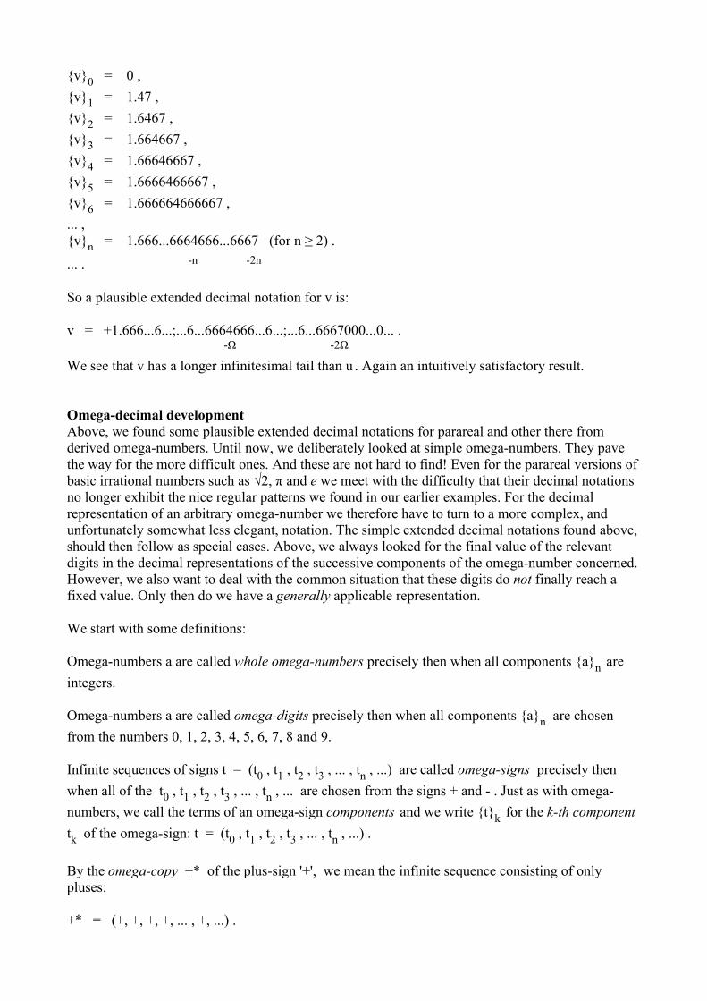
{v}0 = 0 , {v}1 = 1.47 , {v}2 = 1.6467 , {v}3 = 1.664667 , {v}4 = 1.66646667 , {v}5 = 1.6666466667 , {v}6 = 1.666664666667 , ... , {v}n = 1.666...6664666...6667 (for n ≥ 2) .

... . -n -2n

So a plausible extended decimal notation for v is:

v = +1.666...6...;...6...6664666...6...;...6...6667000...0... . -Ω -2Ω We see that v has a longer infinitesimal tail than u . Again an intuitively satisfactory result.

Omega-decimal development Above, we found some plausible extended decimal notations for parareal and other there from derived omega-numbers. Until now, we deliberately looked at simple omega-numbers. They pave the way for the more difficult ones. And these are not hard to find! Even for the parareal versions of basic irrational numbers such as √2, π and e we meet with the difficulty that their decimal notations no longer exhibit the nice regular patterns we found in our earlier examples. For the decimal representation of an arbitrary omega-number we therefore have to turn to a more complex, and unfortunately somewhat less elegant, notation. The simple extended decimal notations found above, should then follow as special cases. Above, we always looked for the final value of the relevant digits in the decimal representations of the successive components of the omega-number concerned. However, we also want to deal with the common situation that these digits do not finally reach a fixed value. Only then do we have a generally applicable representation.

We start with some definitions:

Omega-numbers a are called whole omega-numbers precisely then when all components {a}n are integers.

Omega-numbers a are called omega-digits precisely then when all components {a}n are chosen from the numbers 0, 1, 2, 3, 4, 5, 6, 7, 8 and 9.

Infinite sequences of signs t = (t0 , t1 , t2 , t3 , ... , tn , ...) are called omega-signs precisely then when all of the t0 , t1 , t2 , t3 , ... , tn , ... are chosen from the signs + and - . Just as with omega-numbers, we call the terms of an omega-sign components and we write {t}k for the k-th component tk of the omega-sign: t = (t0 , t1 , t2 , t3 , ... , tn , ...) .

By the omega-copy +* of the plus-sign '+', we mean the infinite sequence consisting of only pluses:

+* = (+, +, +, +, ... , +, ...) .

By the omega-copy -* of the minus-sign '-', we mean the infinite sequence consisting of only minuses: -* = (-, -, -, -, ... , -, ...) .

Two omega-signs t and t' we consider equal precisely than when for all natural numbers n (including 0) it holds that {t}n = {t'}n . The equality of t and t' we write as: t = t'.

Two omega-signs t and t' we consider finally equal precisely then when there is a natural number N such that {t}n = {t'}n for all natural numbers n > N. The final equalness of t and t' we write as:t ≃ t'.

Perhaps unnecessarily, I want to point out that for the + and - sign we use the following conventions:

a = b for a = + & b = + , a ≠ b for a = + & b = - , a ≠ b for a = - & b = + , a = b for a = - & b = - .

Furthermore, any real number a (as one can easily verify in the mathematical literature) can be written in the decimal form:

a = t ... cn ... c3c2c1c0.c-1c-2c-3 ... c-n ... .

And this in exactly one way, when:

(i) the sign t may only be + or - , (ii) the digits ..., cn ,..., c3 , c2 , c1 , c0 , c-1 , c-2 , c-3 , ..., c-n , ... may only be 0, 1, 2, 3, 4, 5, 6, 7, 8 or 9 , (iii) there is no integer N such that ck = 9 for all k < N , (iv) t = + for the case that ck = 0 for all integers k .

The conditions (iii) and (iv) are added for simplicity and unambiguity. We will call the decimal notation thus defined, the stipulated decimal notation.

Our intention is to generalise the stipulated decimal notation for real numbers to an 'omega-decimal development' for omega-numbers. To do this smoothly, we will designate the sign and the digits of the stipulated decimal notation by a 'real signfunction' rt and a 'real digitfunction' rc respectively. (In Dutch sign = teken, and digit = cijfer.) Which we define as follows:

By the real signfunction rt we mean the "function" that has for each real number a the sign t from the (above mentioned) stipulated decimal notation for a, as image rt(a) .

By the real digitfunction rc we mean the function that for any integer k and each real number a has the digit ck from the (above mentioned) stipulated decimal notation for a, as image rc(k,a) .

Of course, with these definitions, we now for each real number a have:

a = rt(a) ... rc(n,a) ... rc(3,a) rc(2,a) rc(1,a) rc(0,a).rc(-1,a) rc(-2,a) rc(-3,a) ... rc(-n,a) ... .

By generalisation of the real signfunction and the real digitfunction we can now easily find the 'omega-decimal development' for omega-numbers. This goes as follows:

By the omega-signfunction ot we mean the "function" that for each omega-number a has the undermentioned image:

ot(a) = ( rt({a}0 ), rt({a}1 ), rt({a}2 ), rt({a}3 ), ... , rt({a}n ), ...) .

It is clear that the omega-signfunction delivers an omega-sign for each omega-number a.

By the omega-digitfunction oc we mean the function that for each whole omega-number k and each omega-number a has the undermentioned image:

oc(k,a) = ( rc({k}0 ,{a}0 ), rc({k}1 ,{a}1 ), rc({k}2 ,{a}2 ), rc({k}3 ,{a}3 ), ... , rc({k}n ,{a}n ), ...) .

It is also clear that the omega-digitfunction delivers an omega-digit for each whole omega-number k and each omega-number a.

Finally, we for each omega-number a mean by its omega-decimal development the omega-sign t = ot(a) of a, together with all omega-digits cm= oc(m,a) of a. An omega-decimal development - by reason of the many possible indices m - therefore forms a dazzlingly complex object. Nevertheless we might want to give some impression So in practice we may write out a beginning, and suggest the rest by means of the ellipsis. For example, as follows:

a = t ... cn* ... c3* c2* c1* c0* .c-1* c-2* c-3* ... c-n* ... ,

where:

t = ot(a) , ... , cn* = oc( n*, a) , ... , c3* = oc( 3*, a) , c2* = oc( 2*, a) , c1* = oc( 1*, a) , c0* = oc( 0*, a) , c-1* = oc(-1*, a) ,c-2* = oc(-2*, a) , c-3* = oc(-3*, a) ,... , c-n* = oc(-n*, a) , ... .

That is:

a = ot(a) ... oc(n*,a) ... oc(3*,a) oc(2*,a) oc(1*,a) oc(0*,a).oc(-1*,a) oc(-2*,a) oc(-3*,a) ... oc(-n*,a) ... .

Note that we indeed have actually written out only the very beginning of the omega-decimal development. Of the stipulated decimal notation for real numbers we of course also cannot write out all digits. But in that case, the digits still have a relatively neat doubly-infinite sequence of indices:

... , n , ... , 3, 2, 1, 0, -1, -2, -3, ... , -n, ... .

There are - admittedly - infinitely many indices here, but the indices themselves are finite numbers. Moreover, each index in this sequence, has a clear position in relation to all other indices. But for the whole omega-numbers, that act as indices for omega-decimal developments, this no longer holds. There are infinitely great whole omega-numbers such as Ω and -2.Ω+4 . And there are whole omega-numbers such as (1, -1, 2, -2, 3, -3, 4, -4, ...) that are neither greater than 0 , nor smaller than 0 , nor equal to 0 . Thus in omega-decimal developments there are as it were digits with indices that refuse to stand in a row. So always remember that an omega-decimal development not only has omega-digits for the orderly sequence of indices:

... , n* , ... , 3*, 2*, 1*, 0*, -1*, -2*, -3*, ... , -n*, ... ,

but that for an omega-decimal development all whole omega-numbers act as an index for omega-digits. Thus an omega-decimal development indeed has an enormes amount of omega-digits!

An alternative presentation - which we will call the omega-decimal matrix - as it were unrolls ot(a) and the oc(k,a) of the omega-decimal development of an omega-number a , downwards. Let a be an omega-number with:

a = (a0 , a1 , a2 , a3 , ... , an , ...) ,

then a beginning of the omega-decimal matrix of a is:

a = rt(a0 ) ... rc(n,a0 ) ... rc(3,a0 ) rc(2,a0 ) rc(1,a0 ) rc(0,a0 ). rc(-1,a0 ) rc(-2,a0 ) rc(-3,a0 ) ... rc(-n,a0 ) ... rt(a1 ) ... rc(n,a1 ) ... rc(3,a1 ) rc(2,a1 ) rc(1,a1 ) rc(0,a1 ). rc(-1,a1 ) rc(-2,a1 ) rc(-3,a1 ) ... rc(-n,a1 ) ... rt(a2 ) ... rc(n,a2 ) ... rc(3,a2 ) rc(2,a2 ) rc(1,a2 ) rc(0,a2 ). rc(-1,a2 ) rc(-2,a2 ) rc(-3,a2 ) ... rc(-n,a2 ) ... rt(a3 ) ... rc(n,a3 ) ... rc(3,a3 ) rc(2,a3 ) rc(1,a3 ) rc(0,a3 ). rc(-1,a3 ) rc(-2,a3 ) rc(-3,a3 ) ... rc(-n,a3 ) ... ... rt(an ) ... rc(n,an ) ... rc(3,an ) rc(2,an ) rc(1,an ) rc(0,an ). rc(-1,an ) rc(-2,an ) rc(-3,an ) ... rc(-n,an ) ... ... .

Because these are precisely the stipulated decimal notations for a0 , a1 , a2 , a3 , ... , an , ... , any omega-number a can be recovered from its omega-decimal matrix, and hence from its omega-decimal development. Thus two different omega-numbers can never have the same omega-decimal development.

What parts of the omega-decimal development we will actually want to write out all depends on the problems in which we are interested. What we still want to do here, is to compare the earlier heuristically found plausible extended decimal notations of our chosen simple omega-numbers with their representation by means of the generally applicable omega-decimal development. The undermentioned explications of parts of the omega-decimal development are specially tailored to this purpose.

Let a be an arbitrary omega-number with:

a = (a0 , a1 , a2 , a3 , ... , an , ...) ,

and let :

t ...c3*c2*c1*c0* .c-1*c-2*c-3* ...;...c-Ω+3c-Ω+2c-Ω+1c-Ωc-Ω-1c-Ω-2c-Ω-3 ...;...c-2Ω+3c-2Ω+2c-2Ω+1c-2Ωc-2Ω-1c-2Ω-2c-2Ω-3 ...;... ,

be (a somewhat bigger chunk from) the omega-decimal development of a .

Then we get:

t = ot(a) = ( rt(a0 ), rt(a1 ), rt(a2 ), rt(a3 ), ... , rt(an ), ...) , ... , c3* = oc( 3*, a) = ( rc( 3, a0 ), rc( 3, a1 ), rc( 3, a2 ), rc( 3, a3 ), ... , rc( 3, an ), ...) , c2* = oc( 2*, a) = ( rc( 2, a0 ), rc( 2, a1 ), rc( 2, a2 ), rc( 2, a3 ), ... , rc( 2, an ), ...) , c1* = oc( 1*, a) = ( rc( 1, a0 ), rc( 1, a1 ), rc( 1, a2 ), rc( 1, a3 ), ... , rc( 1, an ), ...) , c0* = oc( 0*, a) = ( rc( 0, a0 ), rc( 0, a1 ), rc( 0, a2 ), rc( 0, a3 ), ... , rc( 0, an ), ...) , c-1* = oc(-1*, a) = ( rc(-1, a0 ), rc(-1, a1 ), rc(-1, a2 ), rc(-1, a3 ), ... , rc(-1, an ), ...) , c-2* = oc(-2*, a) = ( rc(-2, a0 ), rc(-2, a1 ), rc(-2, a2 ), rc(-2, a3 ), ... , rc(-2, an ), ...) , c-3* = oc(-3*, a) = ( rc(-3, a0 ), rc(-3, a1 ), rc(-3, a2 ), rc(-3, a3 ), ... , rc(-3, an ), ...) , ... , ... , c-Ω+3 = oc(-Ω+3, a) = ( rc( 3, a0 ), rc( 2, a1 ), rc( 1, a2 ), rc( 0, a3 ), ... , rc(-n+3, an ), ...) , c-Ω+2 = oc(-Ω+2, a) = ( rc( 2, a0 ), rc( 1, a1 ), rc( 0, a2 ), rc(-1, a3 ), ... , rc(-n+2, an ), ...) , c-Ω+1 = oc(-Ω+1, a) = ( rc( 1, a0 ), rc( 0, a1 ), rc(-1, a2 ), rc(-2, a3 ), ... , rc(-n+1, an ), ...) , c-Ω = oc(-Ω, a) = ( rc( 0, a0 ), rc(-1, a1 ), rc(-2, a2 ), rc(-3, a3 ), ... , rc(-n, an ), ...) , c-Ω-1 = oc(-Ω-1, a) = ( rc(-1, a0 ), rc(-2, a1 ), rc(-3, a2 ), rc(-4, a3 ), ... , rc(-n-1, an ), ...) , c-Ω-2 = oc(-Ω-2, a) = ( rc(-2, a0 ), rc(-3, a1 ), rc(-4, a2 ), rc(-5, a3 ), ... , rc(-n-2, an ), ...) , c-Ω-3 = oc(-Ω-3, a) = ( rc(-3, a0 ), rc(-4, a1 ), rc(-5, a2 ), rc(-6, a3 ), ... , rc(-n-3, an ), ...) , ... , ... , c-2Ω+3 = oc(-2Ω+3, a) = ( rc( 3, a0 ), rc( 1, a1 ), rc(-1, a2 ), rc(-3, a3 ), ... , rc(-2n+3, an ), ...) , c-2Ω+2 = oc(-2Ω+2, a) = ( rc( 2, a0 ), rc( 0, a1 ), rc(-2, a2 ), rc(-4, a3 ), ... , rc(-2n+2, an ), ...) , c-2Ω+1 = oc(-2Ω+1, a) = ( rc( 1, a0 ), rc(-1, a1 ), rc(-3, a2 ), rc(-5, a3 ), ... , rc(-2n+1, an ), ...) , c-2Ω = oc(-2Ω, a) = ( rc( 0, a0 ), rc(-2, a1 ), rc(-4, a2 ), rc(-6, a3 ), ... , rc(-2n, an ), ...) , c-2Ω-1 = oc(-2Ω-1, a) = ( rc(-1, a0 ), rc(-3, a1 ), rc(-5, a2 ), rc(-7, a3 ), ... , rc(-2n-1, an ), ...) , c-2Ω-2 = oc(-2Ω-2, a) = ( rc(-2, a0 ), rc(-4, a1 ), rc(-6, a2 ), rc(-8, a3 ), ... , rc(-2n-2, an ), ...) , c-2Ω-3 = oc(-2Ω-3, a) = ( rc(-3, a0 ), rc(-5, a1 ), rc(-7, a2 ), rc(-9, a3 ), ... , rc(-2n-3, an ), ...) , ... , ... .

Let again a be an arbitrary omega-number with:

a = (a0 , a1 , a2 , a3 , ... , an , ...) ,

and (for a positive natural number k) let:

t ...c3* c2* c1* c0* .c-1* c-2* c-3* ...;...c-kΩ+3 c-kΩ+2 c-kΩ+1 c-kΩ c-kΩ-1 c-kΩ-2 c-kΩ-3 ...;... ,

also be a piece from the omega-decimal development of a .

Then:

t = ot(a) = ( rt(a0 ), rt(a1 ), rt(a2 ), rt(a3 ), ... , rt(an ), ...) , ... , c3* = oc( 3*, a) = ( rc( 3, a0 ), rc( 3, a1 ), rc( 3, a2 ), rc( 3, a3 ), ... , rc( 3, an ), ...) , c2* = oc( 2*, a) = ( rc( 2, a0 ), rc( 2, a1 ), rc( 2, a2 ), rc( 2, a3 ), ... , rc( 2, an ), ...) , c1* = oc( 1*, a) = ( rc( 1, a0 ), rc( 1, a1 ), rc( 1, a2 ), rc( 1, a3 ), ... , rc( 1, an ), ...) , c0* = oc( 0*, a) = ( rc( 0, a0 ), rc( 0, a1 ), rc( 0, a2 ), rc( 0, a3 ), ... , rc( 0, an ), ...) , c-1* = oc(-1*, a) = ( rc(-1, a0 ), rc(-1, a1 ), rc(-1, a2 ), rc(-1, a3 ), ... , rc(-1, an ), ...) , c-2* = oc(-2*, a) = ( rc(-2, a0 ), rc(-2, a1 ), rc(-2, a2 ), rc(-2, a3 ), ... , rc(-2, an ), ...) , c-3* = oc(-3*, a) = ( rc(-3, a0 ), rc(-3, a1 ), rc(-3, a2 ), rc(-3, a3 ), ... , rc(-3, an ), ...) , ... , ... , c-kΩ+3 = oc(-kΩ+3, a) = ( rc( 3, a0 ), rc(-k+3, a1 ), rc(-2k+3, a2 ), rc(-3k+3, a3 ), ...) , c-kΩ+2 = oc(-kΩ+2, a) = ( rc( 2, a0 ), rc(-k+2, a1 ), rc(-2k+2, a2 ), rc(-3k+2, a3 ), ...) , c-kΩ+1 = oc(-kΩ+1, a) = ( rc( 1, a0 ), rc(-k+1, a1 ), rc(-2k+1, a2 ), rc(-3k+1, a3 ), ...) , c-kΩ = oc(-kΩ, a) = ( rc( 0, a0 ), rc(-k, a1 ), rc(-2k, a2 ), rc(-3k, a3 ), ...) , c-kΩ-1 = oc(-kΩ-1, a) = ( rc(-1, a0 ), rc(-k-1, a1 ), rc(-2k-1, a2 ), rc(-3k-1, a3 ), ...) , c-kΩ-2 = oc(-kΩ-2, a) = ( rc(-2, a0 ), rc(-k-2, a1 ), rc(-2k-2, a2 ), rc(-3k-2, a3 ), ...) , c-kΩ-3 = oc(-kΩ-3, a) = ( rc(-3, a0 ), rc(-k-3, a1 ), rc(-2k-3, a2 ), rc(-3k-3, a3 ), ...) , ... , ... .

We will use the formulas found above, in a moment. However, readers interested in other parts of the omega-decimal development may now easily find the formulas for these other parts themselves. They just follow from the definition of the omega-decimal development.

Examples Previously, we found as plausible extended decimal notations for some simple omega-numbers:

(i) d* = +0.000...0...;...0...0001000...0... . -Ω (ii) (d*)m = +0.000...0...;...0...0001000...0... . -mΩ (iii) «+0.999...9...» = +0.999...9...;...9...9999000...0... . -Ω (iv) «+0.333...3...» = +0.333...3...;...3...3333000...0... . -Ω (v) «+5.000...0...».«+0.333...3...» = +1.666...6...;...6...6665000...0... . -Ω (vi) «+4.999...9...».«+0.333...3...» = +1.666...6...;...6...6664666...6...;...6...6667000...0... . -Ω -2Ω We will now show that these heuristic results are preserved when using the omega-decimal development.

(i) For d* we know that:

d* = (1, 0.1, 0.01, 0.001, 0.0001, 0.00001, 0.000001, ...) .

Written differently:

{d*}0 = + ...0001.000000000... , {d*}1 = + ...0000.100000000... , {d*}2 = + ...0000.010000000... , {d*}3 = + ...0000.001000000... , {d*}4 = + ...0000.000100000... , {d*}5 = + ...0000.000010000... , {d*}6 = + ...0000.000001000... , ... .

So:

t = (+, +, +, +, ... , +, ...) ≃ +* , ... , c3* = (0, 0, 0, 0, 0, 0, 0, 0, 0, 0, ...) ≃ 0*, c2* = (0, 0, 0, 0, 0, 0, 0, 0, 0, 0, ...) ≃ 0*,

c1* = (0, 0, 0, 0, 0, 0, 0, 0, 0, 0, ...) ≃ 0*, c0* = (1, 0, 0, 0, 0, 0, 0, 0, 0, 0, ...) ≃ 0*,

c-1* = (0, 1, 0, 0, 0, 0, 0, 0, 0, 0, ...) ≃ 0*, c-2* = (0, 0, 1, 0, 0, 0, 0, 0, 0, 0, ...) ≃ 0*,

c-3* = (0, 0, 0, 1, 0, 0, 0, 0, 0, 0, ...) ≃ 0*,... , ... , c-Ω+3 = (0, 0, 0, 0, 0, 0, 0, 0, 0, 0, ...) ≃ 0*,

c-Ω+2 = (0, 0, 0, 0, 0, 0, 0, 0, 0, 0, ...) ≃ 0*, c-Ω+1 = (0, 0, 0, 0, 0, 0, 0, 0, 0, 0, ...) ≃ 0*,

c-Ω = (1, 1, 1, 1, 1, 1, 1, 1, 1, 1, ...) ≃ 1*, c-Ω-1 = (0, 0, 0, 0, 0, 0, 0, 0, 0, 0, ...) ≃ 0*

c-Ω-2 = (0, 0, 0, 0, 0, 0, 0, 0, 0, 0, ...) ≃ 0* c-Ω-3 = (0, 0, 0, 0, 0, 0, 0, 0, 0, 0, ...) ≃ 0*... , ... , c-2Ω+3 = (0, 0, 0, 1, 0, 0, 0, 0, 0, 0, ...) ≃ 0*, c-2Ω+2 = (0, 0, 1, 0, 0, 0, 0, 0, 0, 0, ...) ≃ 0*,

c-2Ω+1 = (0, 1, 0, 0, 0, 0, 0, 0, 0, 0, ...) ≃ 0*, c-2Ω = (1, 0, 0, 0, 0, 0, 0, 0, 0, 0, ...) ≃ 0*,

c-2Ω-1 = (0, 0, 0, 0, 0, 0, 0, 0, 0, 0, ...) ≃ 0*,

c-2Ω-2 = (0, 0, 0, 0, 0, 0, 0, 0, 0, 0, ...) ≃ 0*,

c-2Ω-3 = (0, 0, 0, 0, 0, 0, 0, 0, 0, 0, ...) ≃ 0*, ... , ... .

Which agrees with:

d* = +0.000...0...;...0...0001000...0... . -Ω

(ii) For (d*)m it holds (for positive natural numbers m) that:

(d*)m = (100 , 10-1 , 10-2 , 10-3 , ... , 10-n , ...)m , (d*)m = ((100 )m , (10-1 )m , (10-2 )m , (10-3 )m , ... , (10-n )m , ...) , (d*)m = (1, 10-m , 10-2m , 10-3m , ... , 10-nm , ...) , (d*)m = (1, 0.000...001, 0.000...001, 0.000...001, ... , 0.000...001, ...) . -m -2m -3m -nm Written differently:

{(d*)m }0 = + ...0001.0000000000... ,

{(d*)m }1 = + ...0000.000...001000... ,

-m {(d*)m }2 = + ...0000.000...001000... ,

-2m {(d*)m }3 = + ...0000.000...001000... ,

-3m ... ,

{(d*)m }n = + ...0000.000...001000... ,

-nm ... .

So:

t = (+, +, +, +, ... , +, ...) ≃ +* , ... , c3* = (0, 0, 0, 0, 0, 0, 0, 0, 0, 0, ...) ≃ 0*, c2* = (0, 0, 0, 0, 0, 0, 0, 0, 0, 0, ...) ≃ 0*,

c1* = (0, 0, 0, 0, 0, 0, 0, 0, 0, 0, ...) ≃ 0*, c0* = (1, 0, 0, 0, 0, 0, 0, 0, 0, 0, ...) ≃ 0*,

c-1* = (0, ?, 0, 0, 0, 0, 0, 0, 0, 0, ...) ≃ 0*,c-2* = (0, ?, ?, 0, 0, 0, 0, 0, 0, 0, ...) ≃ 0*,

c-3* = (0, ?, ?, ?, 0, 0, 0, 0, 0, 0, ...) ≃ 0*,

... ,

... , c-mΩ+3 = (0, 0, 0, 0, 0, 0, 0, 0, 0, 0, ...) ≃ 0*,

c-mΩ+2 = (0, 0, 0, 0, 0, 0, 0, 0, 0, 0, ...) ≃ 0*, c-mΩ+1 = (0, 0, 0, 0, 0, 0, 0, 0, 0, 0, ...) ≃ 0*,

c-mΩ = (1, 1, 1, 1, 1, 1, 1, 1, 1, 1, ...) ≃ 1*, c-mΩ-1 = (0, 0, 0, 0, 0, 0, 0, 0, 0, 0, ...) ≃ 0*,

c-mΩ-2 = (0, 0, 0, 0, 0, 0, 0, 0, 0, 0, ...) ≃ 0*, c-mΩ-3 = (0, 0, 0, 0, 0, 0, 0, 0, 0, 0, ...) ≃ 0*, ... , ... .

To find the numbers on the places with the question marks, we have to know the exact value of m. But this is irrelevant for establishing the connection with the previously found plausible extended decimal notation for (d*)m. As we see, the omega-sign and the relevant omega-digits are finally equal to omega-copies of the sign and digits of the extended decimal notation:

(d*)m = +0.000...0...;...0...0001000...0... . -mΩ

(iii) For «+0.999...9...» we per definition have:

«+0.999...9...» = (0, 0.9, 0.99, 0.999, 0.9999, 0.99999, 0.999999, ...) .

Differently written:

{«+0.999...9...»}0 = + ...0000.000000000... , {«+0.999...9...»}1 = + ...0000.900000000... , {«+0.999...9...»}2 = + ...0000.990000000... , {«+0.999...9...»}3 = + ...0000.999000000... , {«+0.999...9...»}4 = + ...0000.999900000... , {«+0.999...9...»}5 = + ...0000.999990000... , {«+0.999...9...»}6 = + ...0000.999999000... , ... .

So:

t = (+, +, +, +, +, +, +, +, +, +, ...) ≃ +* , ... , c3* = (0, 0, 0, 0, 0, 0, 0, 0, 0, 0, ...) ≃ 0* ,

c2* = (0, 0, 0, 0, 0, 0, 0, 0, 0, 0, ...) ≃ 0* , c1* = (0, 0, 0, 0, 0, 0, 0, 0, 0, 0, ...) ≃ 0* ,

c0* = (0, 0, 0, 0, 0, 0, 0, 0, 0, 0, ...) ≃ 0* , c-1* = (0, 9, 9, 9, 9, 9, 9, 9, 9, 9, ...) ≃ 9* ,

c-2* = (0, 0, 9, 9, 9, 9, 9, 9, 9, 9, ...) ≃ 9* ,

c-3* = (0, 0, 0, 9, 9, 9, 9, 9, 9, 9, ...) ≃ 9* , ... , ... , c-Ω+3 = (0, 0, 0, 0, 9, 9, 9, 9, 9, 9, ...) ≃ 9* ,

c-Ω+2 = (0, 0, 0, 9, 9, 9, 9, 9, 9, 9, ...) ≃ 9* , c-Ω+1 = (0, 0, 9, 9, 9, 9, 9, 9, 9, 9, ...) ≃ 9* ,

c-Ω = (0, 9, 9, 9, 9, 9, 9, 9, 9, 9, ...) ≃ 9* , c-Ω-1 = (0, 0, 0, 0, 0, 0, 0, 0, 0, 0, ...) ≃ 0* ,

c-Ω-2 = (0, 0, 0, 0, 0, 0, 0, 0, 0, 0, ...) ≃ 0* , c-Ω-3 = (0, 0, 0, 0, 0, 0, 0, 0, 0, 0, ...) ≃ 0* , ... , ... , c-2Ω+3 = (0, 0, 9, 9, 0, 0, 0, 0, 0, 0, ...) ≃ 0* , c-2Ω+2 = (0, 0, 9, 0, 0, 0, 0, 0, 0, 0, ...) ≃ 0* ,

c-2Ω+1 = (0, 9, 0, 0, 0, 0, 0, 0, 0, 0, ...) ≃ 0* , c-2Ω = (0, 0, 0, 0, 0, 0, 0, 0, 0, 0, ...) ≃ 0* ,

c-2Ω-1 = (0, 0, 0, 0, 0, 0, 0, 0, 0, 0, ...) ≃ 0* , c-2Ω-2 = (0, 0, 0, 0, 0, 0, 0, 0, 0, 0, ...) ≃ 0* ,

c-2Ω-3 = (0, 0, 0, 0, 0, 0, 0, 0, 0, 0, ...) ≃ 0* , ... , ... .

Which agrees with:

«+0.999...9...» = +0.999...9...;...9...9999000...0... . -Ω

(iv) For «+0.333...3...» we per definition have:

«+0.333...3...» = (0, 0.3, 0.33, 0.333, 0.3333, 0.33333, 0.333333, ...) .

Differently written:

{«+0.333...3...»}0 = + ...0000.000000000... , {«+0.333...3...»}1 = + ...0000.300000000... , {«+0.333...3...»}2 = + ...0000.330000000... , {«+0.333...3...»}3 = + ...0000.333000000... , {«+0.333...3...»}4 = + ...0000.333300000... , {«+0.333...3...»}5 = + ...0000.333330000... , {«+0.333...3...»}6 = + ...0000.333333000... , ... .

So:

t = (+, +, +, +, +, +, +, +, +, +, ...) ≃ +* , ... , c3* = (0, 0, 0, 0, 0, 0, 0, 0, 0, 0, ...) ≃ 0* ,

c2* = (0, 0, 0, 0, 0, 0, 0, 0, 0, 0, ...) ≃ 0* , c1* = (0, 0, 0, 0, 0, 0, 0, 0, 0, 0, ...) ≃ 0* ,

c0* = (0, 0, 0, 0, 0, 0, 0, 0, 0, 0, ...) ≃ 0* , c-1* = (0, 3, 3, 3, 3, 3, 3, 3, 3, 3, ...) ≃ 3* ,

c-2* = (0, 0, 3, 3, 3, 3, 3, 3, 3, 3, ...) ≃ 3* , c-3* = (0, 0, 0, 3, 3, 3, 3, 3, 3, 3, ...) ≃ 3* , ... , ... , c-Ω+3 = (0, 0, 0, 0, 3, 3, 3, 3, 3, 3, ...) ≃ 3* , c-Ω+2 = (0, 0, 0, 3, 3, 3, 3, 3, 3, 3, ...) ≃ 3* ,

c-Ω+1 = (0, 0, 3, 3, 3, 3, 3, 3, 3, 3, ...) ≃ 3* , c-Ω = (0, 3, 3, 3, 3, 3, 3, 3, 3, 3, ...) ≃ 3* ,

c-Ω-1 = (0, 0, 0, 0, 0, 0, 0, 0, 0, 0, ...) ≃ 0* , c-Ω-2 = (0, 0, 0, 0, 0, 0, 0, 0, 0, 0, ...) ≃ 0* ,

c-Ω-3 = (0, 0, 0, 0, 0, 0, 0, 0, 0, 0, ...) ≃ 0* , ... , ... , c-2Ω+3 = (0, 0, 3, 3, 0, 0, 0, 0, 0, 0, ...) ≃ 0* ,

c-2Ω+2 = (0, 0, 3, 0, 0, 0, 0, 0, 0, 0, ...) ≃ 0* , c-2Ω+1 = (0, 3, 0, 0, 0, 0, 0, 0, 0, 0, ...) ≃ 0* ,

c-2Ω = (0, 0, 0, 0, 0, 0, 0, 0, 0, 0, ...) ≃ 0* , c-2Ω-1 = (0, 0, 0, 0, 0, 0, 0, 0, 0, 0, ...) ≃ 0* ,

c-2Ω-2 = (0, 0, 0, 0, 0, 0, 0, 0, 0, 0, ...) ≃ 0* , c-2Ω-3 = (0, 0, 0, 0, 0, 0, 0, 0, 0, 0, ...) ≃ 0* , ... , ... .

Which agrees with:

«+0.333...3...» = +0.333...3...;...3...3333000...0... . -Ω

(v) For «+5.000...0...».«+0.333...3...» we found:

«+5.000...0...».«+0.333...3...» = (0, 1.5, 1.65, 1.665, ... , 1.666...65 (for n ≥ 2), ...) . -n Written differently:

{«+5.000...0...».«+0.333...3...»}0 = + ...0000.000000000... , {«+5.000...0...».«+0.333...3...»}1 = + ...0001.500000000... , {«+5.000...0...».«+0.333...3...»}2 = + ...0001.650000000... , {«+5.000...0...».«+0.333...3...»}3 = + ...0001.665000000... , ... , {«+5.000...0...».«+0.333...3...»}n = + ...0001.666...65000... (for n ≥ 2) ,

... . -n

So:

t = (+, +, +, +, +, +, +, +, +, +, ...) ≃ +* , ... , c3* = (0, 0, 0, 0, 0, 0, 0, 0, 0, 0, ...) ≃ 0* , c2* = (0, 0, 0, 0, 0, 0, 0, 0, 0, 0, ...) ≃ 0* ,

c1* = (0, 0, 0, 0, 0, 0, 0, 0, 0, 0, ...) ≃ 0* , c0* = (0, 1, 1, 1, 1, 1, 1, 1, 1, 1, ...) ≃ 1* ,

c-1* = (0, 5, 6, 6, 6, 6, 6, 6, 6, 6, ...) ≃ 6* ,c-2* = (0, 0, 5, 6, 6, 6, 6, 6, 6, 6, ...) ≃ 6* ,

c-3* = (0, 0, 0, 5, 6, 6, 6, 6, 6, 6, ...) ≃ 6* , ... , ... , c-Ω+3 = (0, 0, 0, 1, 6, 6, 6, 6, 6, 6, ...) ≃ 6* ,

c-Ω+2 = (0, 0, 1, 6, 6, 6, 6, 6, 6, 6, ...) ≃ 6* , c-Ω+1 = (0, 1, 6, 6, 6, 6 ,6, 6, 6, 6, ...) ≃ 6* ,

c-Ω = (0, 5, 5, 5, 5, 5, 5, 5, 5, 5, ...) ≃ 5* , c-Ω-1 = (0, 0, 0, 0, 0, 0, 0, 0, 0, 0, ...) ≃ 0* ,

c-Ω-2 = (0, 0, 0, 0, 0, 0, 0, 0, 0, 0, ...) ≃ 0* , c-Ω-3 = (0, 0, 0, 0, 0, 0, 0, 0, 0, 0, ...) ≃ 0* , ... , ... , c-2Ω+3 = (0, 0, 6, 5, 0, 0, 0, 0, 0, 0, ...) ≃ 0* , c-2Ω+2 = (0, 1, 5, 0, 0, 0, 0, 0, 0, 0, ...) ≃ 0* ,

c-2Ω+1 = (0, 5, 0, 0, 0, 0, 0, 0, 0, 0, ...) ≃ 0* , c-2Ω = (0, 0, 0, 0, 0, 0, 0, 0, 0, 0, ...) ≃ 0* ,

c-2Ω-1 = (0, 0, 0, 0, 0, 0, 0, 0, 0, 0, ...) ≃ 0* , c-2Ω-2 = (0, 0, 0, 0, 0, 0, 0, 0, 0, 0, ...) ≃ 0* ,

c-2Ω-3 = (0, 0, 0, 0, 0, 0, 0, 0, 0, 0, ...) ≃ 0* , ... , ... .

Which agrees with:

«+5.000...0...».«+0.333...3...» = +1.666...6...;...6...6665000...0... . -Ω

(vi) For «+4.999...9...».«+0.333...3...» we found:

{«+4.999...9...».«+0.333...3...»}0 = 0 , {«+4.999...9...».«+0.333...3...»}1 = 1.47 , {«+4.999...9...».«+0.333...3...»}2 = 1.6467 , {«+4.999...9...».«+0.333...3...»}3 = 1.664667 , {«+4.999...9...».«+0.333...3...»}4 = 1.66646667 , {«+4.999...9...».«+0.333...3...»}5 = 1.6666466667 , {«+4.999...9...».«+0.333...3...»}6 = 1.666664666667 , ... , {«+4.999...9...».«+0.333...3...»}n = 1.666...6664666...6667 (for n ≥ 2) ,

... . -n -2n

Differently written:

{«+4.999...9...».«+0.333...3...»}0 = + ...0000.00000000000000000000... , {«+4.999...9...».«+0.333...3...»}1 = + ...0001.47000000000000000000... , {«+4.999...9...».«+0.333...3...»}2 = + ...0001.64670000000000000000... , {«+4.999...9...».«+0.333...3...»}3 = + ...0001.66466700000000000000... , {«+4.999...9...».«+0.333...3...»}4 = + ...0001.66646667000000000000... , {«+4.999...9...».«+0.333...3...»}5 = + ...0001.66664666670000000000... , {«+4.999...9...».«+0.333...3...»}6 = + ...0001.66666466666700000000... , ... , {«+4.999...9...».«+0.333...3...»}n = + ...0001.666...6664666...6667000... (for n ≥ 2) , ... . -n -2n

So:

t = (+, +, +, +, +, +, +, +, +, +, ...) ≃ +* , ... , c3* = (0, 0, 0, 0, 0, 0, 0, 0, 0, 0, ...) ≃ 0* ,

c2* = (0, 0, 0, 0, 0, 0, 0, 0, 0, 0, ...) ≃ 0* , c1* = (0, 0, 0, 0, 0, 0, 0, 0, 0, 0, ...) ≃ 0* ,

c0* = (0, 1, 1, 1, 1, 1, 1, 1, 1, 1, ...) ≃ 1* , c-1* = (0, 4, 6, 6, 6, 6, 6, 6, 6, 6, ...) ≃ 6* ,

c-2* = (0, 7, 4, 6, 6, 6, 6, 6, 6, 6, ...) ≃ 6* , c-3* = (0, 0, 6, 4, 6, 6, 6, 6, 6, 6, ...) ≃ 6* ,... , ... , c-Ω+3 = (0, 0, 0, 1, 6, 6, 6, 6, 6, 6, ...) ≃ 6* ,

c-Ω+2 = (0, 0, 1, 6, 6, 6, 6, 6, 6, 6, ...) ≃ 6* ,

c-Ω+1 = (0, 1, 6, 6, 6, 6, 6, 6, 6, 6, ...) ≃ 6* , c-Ω = (0, 4, 4, 4, 4, 4, 4, 4, 4, 4, ...) ≃ 4* ,

c-Ω-1 = (0, 7, 6, 6, 6, 6, 6, 6, 6, 6, ...) ≃ 6* , c-Ω-2 = (0, 0, 7, 6, 6, 6, 6, 6, 6, 6, ...) ≃ 6* ,

c-Ω-3 = (0, 0, 0, 7, 6, 6, 6, 6, 6, 6, ...) ≃ 6* , ... , ... , c-2Ω+3 = (0, 0, 6, 4, 6, 6, 6, 6, 6, 6, ...) ≃ 6* ,

c-2Ω+2 = (0, 1, 4, 6, 6, 6, 6, 6, 6, 6, ...) ≃ 6* , c-2Ω+1 = (0, 4, 6, 6, 6, 6, 6, 6, 6, 6, ...) ≃ 6* ,

c-2Ω = (0, 7, 7, 7, 7, 7, 7, 7, 7, 7, ...) ≃ 7* , c-2Ω-1 = (0, 0, 0, 0, 0, 0, 0, 0, 0, 0, ...) ≃ 0* ,

c-2Ω-2 = (0, 0, 0, 0, 0, 0, 0, 0, 0, 0, ...) ≃ 0* , c-2Ω-3 = (0, 0, 0, 0, 0, 0, 0, 0, 0, 0, ...) ≃ 0* , ... , ... .

Which agrees with:

«+4.999...9...».«+0.333...3...» = +1.666...6...;...6...6664666...6...;...6...6667000...0... . -Ω -2Ω All in all, the omega-decimal development is seen to be a neatly defined generalisation of the earlier heuristically found extended decimal notations for some simple omega-numbers.

Escultura's new real numbers and the parareal numbers In a previous article [3] we discussed the attempt by Professor Edgar E. Escultura to design a number system (called the new real numbers ) with 0.999... ≠ 1. As it now appears the system of Schmieden and Laugwitz already has this possibility. Indeed we found: «+1.000...0...» = «+0.999...9...» + d*. Here «+1.000...0...» and «+0.999...9...» are what we have called parareal numbers, and d* is an infinitesimal omega-number. Nevertheless, our d* has not exactly the same properties that Escultura attributes to his d*. Thus, according to Escultura (see [4]) for all natural numbers n > 2 we should have:

xn + yn = zn ,

when:

x = (0.999...).10T , y = d*, z = 10T ,

for all positive natural numbers T.

Let us take a look at the simplest case: n = 3 and T = 1. For our parareal numbers and for the infinitesimal omega-number d* we then get:

x = «+0.999...9...».«+10.000...0...», y = d* , z = «+10.000...0...».

So: {x}k = {«+0.999...9...».«+10.000...0...»}k , {x}k = {«+0.999...9...»}k . {«+10.000...0...»}k ,

{x}k = (1 - 10-k ) .10 .

{y}k = {d*}k ,

{y}k = 10-k .

{z}k = {«+10.000...0...»}k . {z}k = 10 .

Hence:

{x3 + y3}k = {x3}k + {y3}k ,

{x3 + y3}k = {x}k3 + {y}k

3 ,

{x3 + y3}k = ((1 - 10-k ) .10)3 + (10-k

)3 ,

{x3 + y3}k = (1 - 10-k )3 .1000 + (10-k

)3 ,

{x3 + y3}k = (1 - 3.10-k + 3.(10-k )2 - (10-k

)3 ) .1000 + (10-k )3 ,

{x3 + y3}k = 1000 - 3000.10-k + 3000.(10-k )2 - 999.(10-k

)3 .

{z3}k = {z}k 3 ,

{z3}k = 103 ,

{z3}k = 1000 .

It is easy to verify that {x3 + y3}k ≠ {z3}k for k = 0. So we already know that:

x3 + y3 ≠ z3 .

But might there still be infinitely many values of k for which we have: {x3 + y3}k = {z3}k ? For such k we would have:

{x3 + y3}k = {z3}k ,

1000 - 3000.10-k + 3000.(10-k )2 - 999.(10-k

)3 = 1000 , -3000.10-k + 3000.(10-k

)2 - 999.(10-k )3 = 0 ,

-3000 + 3000.10-k - 999.(10-k )2 = 0 .

Since this is a quadratic equation in 10-k and f(k) = 10-k is a strictly decreasing function of k, there can be at most two values of k for which {x3 + y3}k = {z3}k . Thus:

x3 + y3 ≄ z3 .

However, it is clear that: x3 + y3 ≈ z3. But because we also have «+0.999...9...» ≈ 1 and d* ≈ 0, this is nothing special.

Variants For convenience, we based our presentation on sequences of real numbers. As a result, we got a number system that contains all omega-copies of real numbers as well as all parareal numbers. We could also have started with sequences of rational numbers. The construction of the usual real numbers can then be omitted (see [14]). In this way we can get an alternative extension of the system Q of rational numbers. In this alternative system, the parareal numbers (as sequences of terminating decimal and therefore rational numbers) can also be defined. Because this system does not depend on the real numbers, it could possibly be more attractive for people who insist on the inequality of 0.999... and 1 in any system. However, we will not here consider the advantages and disadvantages of such an approach.

Finally, we could also have made use of the non-standard analysis of Abraham Robinson (1918-1974). This theory, just like the omega-analysis of Schmieden and Laugwitz, makes it possibly to introduce infinitely small and infinitely great numbers [13]. One of Robinson's assistants A. Harold Lightstone has even devised a way to give infinitely small numbers a decimal representation [10]. This looks somewhat like our approach, but there are also important differences. Lightstone's approach is of a pronounced non-constructive character. A specific application of Robinson's non-standard analysis to the 0.999... problem is given by Karin Usadi Katz and Mikhail G. Katz in their A Strict Non-standard Inequality .999... < 1 [5]. However, because the foundations of non-standard analysis are extremely abstract, it is doubtful whether a real clarification of the 0.999... problem can thereby be achieved.

Conclusion The above provides a simplified, coarse sketch. I have not followed Schmieden and Laugwitz to closely. My intention has been to present the core of the omega-analysis in a very simple but still sound way. We have not used a rigorous presentation on the basis of definitions and proofs. Although that surely would also have been an interesting exercise! The proofs we did include, however, give some impression. How the omega-analysis as a whole can be developed in a mathematically sound way one can read in [8] and [14].

Nevertheless, I believe to have made it sufficiently clear that it indeed is possible to construct a number system in which 0.999... is smaller than 1. The intuition of many that 0.999... is a 'little' smaller than 1, thus should not simply be dismissed as nonsense. Besides that, the number system here sketched is basically to be understood as a contribution to recreational mathematics. The abundant discussions on the Internet on the 0.999... question frequently run around in circles where long known arguments are endlessly repeated. It would be much more interesting - and also much more fun! - when people would actually start designing and developing alternative number systems in which 0.999... and 1 are unequal. In this area math enthusiasts still have a lot to discover.

Bart van Donselaar

[The original article can be found on http://wetenschap.infonu.nl/wiskunde/35856-omega-analyse-en-0999.html .]

Sources and references:

[1] 0.999... (http://en.wikipedia.org/wiki/0.999).

[2] DeSua, F.C. (1960) A System Isomorphic to the Reals. American Mathematical Monthly 67. pp. 900-903 .

[3] Donselaar, B. van (2009). Edgar E. Escultura en de ongelijkheid van 1 en 0,999... (http://wetenschap.infonu.nl/wiskunde/32165-edgar-e-escultura-en-de-ongelijkheid-van-1-en-0999.html).

[4] Freeman, L. (2006). False Proofs - E.E. Escultura. (http://falseproofs.blogspot.com/).

[5] Katz, K. Usadi & Katz, M. G.(2009). A Strict Non-standard Inequality .999 . . . < 1.(http://arxiv.org/PS_cache/arxiv/pdf/0811/0811.0164v8.pdf).

[6] Laugwitz, D. (1961). Anwendungen unendlich kleiner Zahlen. I. Zur Theorie der Distributionen. Journal für die reine und angewandte Mathematik 207, pp. 53-60.

[7] Laugwitz, D. (1961). Anwendungen unendlich kleiner Zahlen. II. Ein Zugang zur Operatorenrechnung von Mikusiński. Journal für die reine und angewandte Mathematik 208. pp. 22-34.

[8] Laugwitz, D. (1973). Ein Weg zur Nonstandard-Analysis. Jahresbericht der Deutschen Mathematiker-Vereinigung 75 pp. 66-93.

[9] Laugwitz, D. (1984). Rise, Fall and Resurrection of Infinitesimals. Tekst Nr. 88. (http://milne.ruc.dk/ImfufaTekster/pdf/88.pdf).

[10] Lightstone, A. H. (1972). Infinitesimals. American Mathematical Monthly 79, 242–251.

[11] Plutonium, A. (2004). Adics are Riemannian Geometry and Reals are Lobachevsky and Doubly−Infinites are Euclidean Geometry. (http://sci.tech-archive.net/pdf/Archive/sci.logic/2004-09/1103.pdf).

[12] Plutonium, A. (2004). Re: evidence Re: Reals form a saddle shape? Re: Adics are Riemannian Geometry and Reals are Lobachevsky and Doubly−Infinites are Euclidean. (http://sci.tech-archive.net/pdf/Archive/sci.math/2004-09/4247.pdf).

[13] Robinson, A. (1996). Non-standard Analysis. Princeton, New Jersey: Princeton University Press.

[14] Schmieden, C. & Laugwitz, D. (1958). Eine Erweiterung der Infinitesimalrechnung Mathematische Zeitschrift 69, pp. 1-39.

[15] Spalt, D.D. (1981). Vom Mythos der mathematischen Vernunft. Darmstadt: Wissenschaftliche Buchgesellschaft.

[16] Vollrath, H.-J. (1968). Grundgedanken der Omega-Analysis und ihrer Anwendung auf die Bestimmung reeller Grenzwerte. Mathematisch Physikalische Semesterberichte 15, pp. 102-111.