Rough Sets and its Different Applications

Faculty of EducationMathematics Department

Rough Sets and its Different Applications

A Thesis

Submitted in Partial Fulfillment of the Requirements of the Master’s

Degree in Teacher’s Preparation in Science

(Pure Mathematics)

Submitted to:

The Department of Mathematics, Faculty of Education, Ain Shams

Universty

By

Amr Zakaria Mohamed Abd El-Hamed

Demonstrator at,

Mathematics Department, Faculty of Education, Ain Shams

Universty

Supervised by

Prof. Dr. Ali Kandil Saad Ibrahim Dr. Mohamed Mostafa YakoutProfessor of Pure Mathematics Lecturer of Pure Mathematics

Department of Mathematics Department of MathematicsFaculty of Science Faculty of EducationHelwan University Ain Shams University

Dr. Emad Hassan AlyLecturer of Applied Mathematics

Department of MathematicsFaculty of EducationAin Shams University

2011

Faculty of EducationDepartment of Mathematics

Candidate: Amr Zakaria Mohamed Abd El-Hamed

Thesis Title: Rough Sets and its Different Applications

Degree: Master’s Degree for Teacher’s Preparation inScience

(Pure Mathematics)

Supervisors:

No. Name Profession Signature

1. Prof. Dr. Ali Kandil Saad Ibrahim Prof. of Pure Mathematics,Department of Mathematics,Faculty of Science,Helwan University.

2. Dr. Mohamed Mostafa Yakout Mousa Lecturer of Pure Mathematics,Department of Mathematics,Faculty of Education,Ain Shams University.

3. Dr. Emad Hassan Aly Lecturer of Applied Mathematics,Department of Mathematics,Faculty of Education,Ain Shams University.

Acknowledgements

I want to start by expressing my deep gratitude to God for giving me

the strength and faith to start this journey and the ability to finally

complete this work.

This thesis would not be possible without the support of many in-

dividuals, to whom I would like to express my gratitude. First and

foremost, I would like to thank my supervisors:

Prof. Dr. Ali Kandil Saad, Professor of Pure Mathematics,

Helwan University, for the opportunity of working with him, and for

his continuous guidance, motivations, and encouragement throughout

my M.S.c studies. His invaluable suggestions and precious ideas have

helped me to walk through various stages of my research, while his

passion and extraordinary dedication to work have always inspired me

and encouraged me to work harder. His trust and support in delega-

tion have instilled in me great confidence and were key factors in my

development as a person and as a researcher.

Dr. Mohamed Mostafa Yakout, Lecturer of Pure Mathemat-

ics, Ain Shams University, for his dedication and guidance during the

elaboration of this thesis. The constant encouragement he provided

was essential for the determination of the course of this work. I am

indebted to him for the time and attention he devoted to this project.

Dr. Emad Hassan Aly, Lecturer of Applied Mathematics, Fac-

ulty of Education, Ain Shams University, who provided me with guid-

ance and continuous encouragement. Dr Aly did his best for the success

3

of this work through seminars, many discussions, precious comments

and valuable reviews and remarks. His efforts during revision of this

thesis is an invaluable.

I would like to thank Prof. Dr. Galal Mahrous, Head of Mathe-

matics Department, Faculty of Education, Ain Shams University, and

all staff members for providing me all facilities required to the success

of this work. I would like to offer my great thanks to all my friends

who helped me through this thesis, especially all colleagues of Prof.

Kandil’s topological seminar for their interest and support.

Finally, words fail me to express my appreciation to my father Za-

karia, my mother Mona, my brothers, Osama, Mohamed, my sisters,

Shimaa, Gehad, Nadia for their support and encouragement through-

out my life.

Amr Zakaria

Summary

A classic paper of Pawlak [23] is the rough sets, published in 1982,

which declared the birth of the Rough Set theory. A lot of mathemati-

cians, logicians, and researchers of computers have become interested

in the rough set theory and have done a lot of research work of rough

set theory in [7, 15, 17] and applications. This is introduced in wide

fields such as machine learning [6], data mining [5], decision making

support and analysis [19, 27, 30], process control [28] and expert system

[43].

The theory of rough sets [11, 21, 25] is a mathematical tool for

extracting knowledge from uncertain and incomplete data based infor-

mation. The theory assumes that we first have necessary information

or knowledge of all the objects in the universe with which the objects

can be divided into different groups. If we have exactly the same infor-

mation of two objects then we say that they are indiscernible (similar),

i.e. we cannot distinguish them with known knowledge. The theory

of rough sets can be used to find dependence relationship among data,

evaluate the importance of attributes, discover the patterns of data,

learn common decision making rules, reduce all redundant objects and

attributes and seek the minimum subset of attributes so as to attain

satisfying classification.

This Thesis includes four chapters as follows:

Chapter 1 is a natural introduction, providing the reader with

results concerning, relations, bitopological spaces, ideals, rough sets,

i

SUMMARY

rough membership function and rough relations.

In Chapter 2, a new definitions of lower and upper approximations

via ideal have been introduced. These new definitions are compared

with Pawlak’s, Yao’s and Allam’s definitions. It’s therefore shown that

the current definitions are more generally. It’s shown that the present

method decreases the boundary region and we get a topology finer

than Allam’s one which is a generalization of that obtained by Yao’s

method. In addition, T1 topological spaces are obtained by relations

and ideals which are not discrete. Moreover, a new rough member-

ship function for any reflexive binary relation R on a non-empty finite

set X is introduced and new lower and upper approximations via this

membership function are defined. We introduce a new rough relation

and its properties.

Some results of this chapter are:

• Published in Annals of Fuzzy Mathematics and Informatics.

• Another results of the current chapter have been submitted for

international Journal.

In Chapter 3, we used preordered relations to define a bipreordered

space and hence bitopological space and introduced a condition

(*): If (R1y ∩R2z)\{y, z} 6= φ, then yR1z or zR2y. On these relations

such that R(A ∪ B) = R(A) ∪ R(B), where R(A) = R1(A) ∩ R2

(A),

and hence we get a topology τR12 on X satisfies

A = R(A) = R1(A)∩R2

(A) = {x ∈ X : xR1∩xR2∩A 6= φ} = A1∩A2

and τR12 = τR1∩R2 = τR1 ∨ τR2 .We deal with bitopological spaces

(X, τ1, τ2) which satisfying a certain condition

(**):({y}1∩{z}

2)\{y, z} 6= φ⇒ y ∈ {z}

1or z ∈ {y}

2and proved that

the family of all such bitopological spaces BTS∗∗ is equivalent to the

family of all bipreordered spaces BPS∗.

ii

SUMMARY

We generate some topologies via different relations and ideals as

cofinite topology, cocountable topology and particular point topology.

Some results of this chapter are:

• Published in Journal of Life Science.

In Chapter 4, a new method via ideal for reduction of attributes

is introduced. Four examples of different sciences are solved, namely

in medicine (cancer and rheumatic fever), environment and automo-

tive sciences. On comparing with an old method [42], it is found that

the present one is better because the number of attributes becomes

smaller than the number of those in the old one or there exist flexibil-

ity of choosing the attributes. In addition, this chapter contains two

appendices, where basic concepts of rough sets for applications have

been introduced in the Appendix A, while the second one, Appendix

B, contains some important definitions and properties of cancer which

have been needed on studying rough sets in breast cancer.

• It should be noted that some results of this chapter have been

prepared for international publication.

iii

SUMMARY

iv

Contents

1 Preliminaries 1

1.1 Relations . . . . . . . . . . . . . . . . . . . . . . . . . . 1

1.2 Some basic concepts of topological

structure . . . . . . . . . . . . . . . . . . . . . . . . . . 2

1.3 Bitopological spaces . . . . . . . . . . . . . . . . . . . . 4

1.4 Ideals . . . . . . . . . . . . . . . . . . . . . . . . . . . 5

1.5 Rough sets . . . . . . . . . . . . . . . . . . . . . . . . . 7

1.5.1 Pawlak’s approximation space . . . . . . . . . . 8

1.5.2 Yao’s approximation space . . . . . . . . . . . . 11

1.5.3 Allam’s approximation space . . . . . . . . . . . 13

1.6 Rough membership function . . . . . . . . . . . . . . . 14

1.7 Rough relations . . . . . . . . . . . . . . . . . . . . . . 16

1.7.1 Properties of rough relations . . . . . . . . . . . 18

2 Generalized Rough Sets, Rough Membership Functions

and Rough Relations 21

2.1 Generalized rough sets via ideals . . . . . . . . . . . . . 22

2.2 Generalized rough membership

function via ideals . . . . . . . . . . . . . . . . . . . . . 29

2.3 Generalized rough relations via ideals . . . . . . . . . . 34

2.4 Properties of rough relations . . . . . . . . . . . . . . . 37

v

CONTENTS

3 On Bipreordered Approximation Spaces 41

3.1 Bipreordered spaces . . . . . . . . . . . . . . . . . . . . 42

3.2 Special kinds of bitopological spaces . . . . . . . . . . . 47

3.3 Generating some topologies via

relations . . . . . . . . . . . . . . . . . . . . . . . . . . 49

3.3.1 Finite case . . . . . . . . . . . . . . . . . . . . . 50

3.3.2 Discrete topology . . . . . . . . . . . . . . . . . 50

3.3.3 Indiscrete topology . . . . . . . . . . . . . . . . 50

3.3.4 Particular point topology . . . . . . . . . . . . . 50

3.3.5 Particular point topology via ideal . . . . . . . 51

3.3.6 Excluded point topology . . . . . . . . . . . . . 51

3.3.7 Inclusion topology . . . . . . . . . . . . . . . . 51

3.3.8 Exclusion topology . . . . . . . . . . . . . . . . 51

3.3.9 Cofinite topology via ideal . . . . . . . . . . . . 52

3.3.10 Cocountable topology via ideal . . . . . . . . . 52

3.3.11 Example . . . . . . . . . . . . . . . . . . . . . . 52

4 Rough Sets and its Applications in Different Sciences 55

4.1 Rough sets in medicine . . . . . . . . . . . . . . . . . . 56

4.1.1 Rough sets in medical data mining . . . . . . . 56

4.1.2 Degree of dependency via ideal . . . . . . . . . 57

4.1.3 Reduction of condition attributes relative to de-

cision attributes via ideal . . . . . . . . . . . . . 57

4.1.4 Rough sets in breast cancer . . . . . . . . . . . 57

4.1.5 Rough sets in rheumatic fever . . . . . . . . . . 61

4.2 Rough sets in environment science . . . . . . . . . . . 62

4.3 Rough sets in automotive science . . . . . . . . . . . . 64

A Basic Concepts of the Rough Sets for Applications 67

A.1 Information system . . . . . . . . . . . . . . . . . . . . 67

A.2 Indiscernibility relation . . . . . . . . . . . . . . . . . . 67

vi

CONTENTS

A.3 Lower and upper approximations . . . . . . . . . . . . 68

A.4 Accuracy of approximation . . . . . . . . . . . . . . . . 69

A.5 The discernibility matrix . . . . . . . . . . . . . . . . . 69

A.6 The discernibility function . . . . . . . . . . . . . . . . 70

A.7 Reduction of knowledge . . . . . . . . . . . . . . . . . 71

A.8 Decision table . . . . . . . . . . . . . . . . . . . . . . . 72

A.9 Degree of dependency . . . . . . . . . . . . . . . . . . . 72

A.10 Reduction of condition attributes relative to decision

attributes [42] . . . . . . . . . . . . . . . . . . . . . . . 72

B Definitions and properties of cancer 73

B.1 Benign and malignant tumors . . . . . . . . . . . . . . 73

B.2 Cancer and normal cells . . . . . . . . . . . . . . . . . 74

Bibliography 77

vii

Chapter 1

Preliminaries

1.1 Relations

Definition 1.1.1 [20] A binary relation from a set X to a set Y is a

subset of X ×Y . If R is a relation, we write (x, y) ∈ R or equivalently

xRy.

Definition 1.1.2 [20] A subset of X × X is a binary relation in the

set X. In particular, the set X ×X is the universal relation in X.

Definition 1.1.3 [20] A relation R in a set X is

1. reflexive if xRx for all x ∈ X,

2. an identity if it is reflexive and if xRy for x, y ∈ X ⇒ x = y,

3. symmetric if xRy for x, y ∈ X ⇒ yRx,

4. antisymmetric if xRy and yRx for x, y ∈ X ⇒ x = y,

5. transitive if xRy and yRz for x, y, z ∈ X ⇒ xRz.

Definition 1.1.4 [47] A reflexive, antisymmetric and transitive rela-

tion in a set is called a partial order in the set. If R is a partial order in

X, the ordered pair (X,R) is called a partially ordered set or a Poset.

1

1.2. SOME BASIC CONCEPTS OF TOPOLOGICALSTRUCTURE

Definition 1.1.5 [20] A relation in a set X is called an equivalence

relation in X if it is reflexive, symmetric and transitive.

1.2 Some basic concepts of topological

structure

Definition 1.2.1 [10] Let X be a non-empty set. A class τ of subsets

of X is called a topology on X iff τ satisfies the following axioms:

1. X,φ ∈ τ ,

2. Arbitrary union of members of τ belongs to τ ,

3. The intersection of any two sets in τ belongs to τ .

The member of τ is then called τ -open set, or simply open set, and the

pair (X, τ) is called a topological space.

A subset A of a topological space (X, τ) is called a closed set if its

complement A′ is an open set.

Definition 1.2.2 [10] Let τ1 and τ2 be two topologies on a set X. τ1

is said to be finer than τ2 or τ2 is said to be coarser than τ1 if every

τ2-open set is τ1-open.

Definition 1.2.3 [13] Let P (X) be the class of all subsets of X. If

h : P (X)→ P (X) is a function satisfying

1. h(φ) = φ,

2. A ∈ P (X)⇒ A ⊆ h(A),

3. A,B ∈ P (X)⇒ h(A ∪B) = h(A) ∪ h(B), and

4. A ∈ P (X)⇒ h(h(A)) = h(A),

2

1.2. SOME BASIC CONCEPTS OF TOPOLOGICALSTRUCTURE

then h is called a Kuratowski’s closure operator and

{A ∈ P (X) : h(A′) = A′}

is a topology on X, where A′ is the complement of A with respect to

X.

Theorem 1.2.1 [13] Let P (X) be the class of all subsets of X. If

K : P (X)→ P (X) is a function satisfying

1. K(φ) = φ,

2. K(A ∪B) = K(A) ∪K(B),

3. K(K(A)) ⊆ K(A).

Then cl : P (X) → P (X) defined by cl(A) := A ∪ K(A) is a Kura-

towski’s closure operator on P (X).

Definition 1.2.4 [10] Let (X, τ) be a topological space and β ⊆ τ .

Then β is called a base for the topology τ iff

1. every open set G ∈ τ is a union of members of β.

Equivalently, β is a base for τ iff

2. for any point p belonging to an open set G, there exists B ∈ βwith p ∈ B ⊆ G.

Theorem 1.2.2 [20] Let β ⊆ P (X). β is a topological basis iff the

following conditions are satisfied:

1. ∪{B : B ∈ β} = X

2. Given B1, B2 ∈ β and x ∈ B1 ∩B2, there exists B ∈ β such that

x ∈ B ⊆ B1 ∩B2.

3

1.3. BITOPOLOGICAL SPACES

1.3 Bitopological spaces

Definition 1.3.1 [8] Let (X, τ1, τ2) be a bitopological space. Then

1. the p∗-closure operator − : P (X)→ P (X) is defined by:

A = A1 ∩ A2

, ∀A ∈ P (X), (1.1)

where Ai

denotes the closure of A w.r.t. τi, i = 1, 2,

2. the p∗-interior operator o : P (X)→ P (X) is defined by:

Ao = Ao1 ∪ Ao2, ∀A ∈ P (X), (1.2)

where Aoi denotes the interior of A w.r.t. τi, i = 1, 2.

Theorem 1.3.1 [9] Let (X, τ1, τ2) be a bitopological space. Then the

p∗-closure and p∗-interior operators satisfy the following properties:

1. A ⊆ A,

2. A ⊆ B ⇒ A ⊆ B,

3. A = A,

4. A ∪B ⊆ A ∪B,

5. A ∩B ⊆ A ∩B,

6. φ = φ,

7. Ao ⊆ A,

8. A ⊆ B ⇒ Ao ⊆ Bo,

9. (A ∩B)o ⊆ Ao ∩Bo,

4

1.4. IDEALS

10. Ao ∪Bo ⊆ (A ∪B)o,

11. Aoo = Ao,

12. Ao′ = A′.

1.4 Ideals

Definition 1.4.1 [13] A non-empty collection I of subsets of a set X

is called an ideal on X, if it satisfies the following conditions

1. A ∈ I and B ∈ I ⇒ A ∪B ∈ I,

2. A ∈ I and B ⊆ A⇒ B ∈ I,

i.e. I is closed under finite unions and subsets.

Example 1.4.1 [13] Let X be a non-empty set. Then the following

families are ideals on X

1. I = {φ},

2. I = P (X) = {A : A ⊆ X},

3. If = {A ⊆ X : A is finite}, called ideal of finite subsets,

4. Ic = {A ⊆ X : A is countable}, called ideal of countable subsets,

5. IA = {B ⊆ X : B ⊆ A},

6. If (X, τ) is a topological space, then the family of nowhere dense

subsets, namely In = {A ⊆ X : Ao

= φ} forms an ideal on X.

It should be noted that the collection of complements of sets in a

proper ideal is a non-empty collection of non-empty sets closed under

the operations of superset and finite intersection. Such a collection is

called a filter; hence an ideal is sometimes called a dual filter.

5

1.4. IDEALS

Definition 1.4.2 [13] Let (X, τ) be a topological space and I be an

ideal on X. Then

A∗(I, τ) (orA∗) := {x ∈ X : Ox ∩ A 6∈ I ∀Ox}

is called the local function of A with respect to I and τ , where Ox is

open set containing x.

Theorem 1.4.1 [13] Let (X, τ) be a topological space with I and Jideals on X, and let A and B be subsets of X. Then

1. A ⊆ B ⇒ A∗ ⊆ B∗,

2. I ⊆ J ⇒ A∗(I) ⊆ A∗(J ),

3. A∗ = cl(A∗) ⊆ cl(A), where cl is the closure w.r.t. τ ,

4. (A∗)∗ ⊆ A∗,

5. (A ∪B)∗ = A∗ ∪B∗,

6. A∗ −B∗ = (A−B)∗ −B∗ ⊆ (A−B)∗,

7. G ∈ τ ⇒ G ∩ A∗ = G ∩ (G ∩ A)∗ ⊆ (G ∩ A)∗,

8. I ∈ I ⇒ (A ∪ I)∗ = A∗ = (A− I)∗.

Proposition 1.4.1 [13] Let (X, τ) be a topological space and I be an

ideal on X. Then the closure operator

cl∗ : P (X)→ P (X)

defined by:

cl∗(A) = A ∪ A∗ (1.3)

satisfies Kuratwski’s axioms and induces a topology on X called τ ∗(I)

given by

τ ∗(I) = {A ⊆ X : cl∗(A′) = A′}. (1.4)

6

1.5. ROUGH SETS

Proposition 1.4.2 [13] Let (X, τ) be a topological space and I be an

ideal on X. Then τ ⊆ τ ∗(I), i.e. τ ∗(I) is finer than τ .

Examples 1.4.1 [13] Let (X, τo) be the indiscrete space. Then

1. If I = If , then τ ∗(If ) = {A ⊆ X : A′ finite} ∪ {φ} known as

the cofinite topology.

2. If I = Ic, then τ ∗(Ic) = {A ⊆ X : A′ countable}∪ {φ} known as

the cocountable topology.

3. If I = I(X−{a}), then

τ ∗(I(X−{a})) = {A ⊆ X : a ∈ A} ∪ {φ}

known as the particular point topology.

Example 1.4.2 [13] Let N be the set of natural numbers and τ be the

partition topology on N generated by the base {{2n − 1, 2n} : n ∈ N}and consider the ideal If . Then τ ∗(If ) is the discrete topology on N.

Theorem 1.4.2 [13] Let (X, τ) be a topological space and I be an

ideal on X. Then

β(I, τ) = {G− I : G ∈ τ, I ∈ I}

is a basis for τ ∗(I).

1.5 Rough sets

The notion of approximation spaces is one of the fundamental con-

cepts in the theory of rough set. This section presents a review of the

Pawlak’s approximation space constructed from an equivalence rela-

tion and its generalization using any binary relations.

7

1.5. ROUGH SETS

1.5.1 Pawlak’s approximation space

Let X denotes a non-empty finite set. Let R be an equivalence rela-

tion on X. The pair apr = (X,R) is called a Pawlak’s approximation

space. The equivalence relation R partitions the set X into disjoint

subsets. Let X/R denotes the quotient set consisting of equivalence

classes of R. The empty set φ and the elements of X/R are called

elementary sets. A finite union of elementary sets is called composed

set [16]. The family of all composed sets is denoted by Com(apr). It

is a subalgebra of the Boolean algebra 2X formed by the power set of

X. A set which is a union of elementary sets is called a definable set

[16]. The family of all definable sets is denoted by Def(apr). For a

finite universe, the family of definable sets is the same as the family

of composed sets. A Pawlak’s approximation space defines uniquely a

topological space (X,Def(apr)), in which Def(apr) is the family of all

open and closed sets [23]. Given an arbitrary set A ⊆ X, in general it

may not be possible to describe A precisely in apr = (X,R). One may

characterize A by a pair of lower and upper approximations.

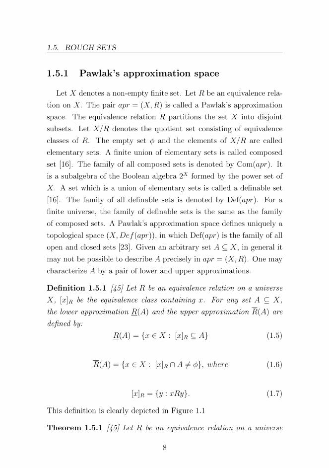
Definition 1.5.1 [45] Let R be an equivalence relation on a universe

X, [x]R be the equivalence class containing x. For any set A ⊆ X,

the lower approximation R(A) and the upper approximation R(A) are

defined by:

R(A) = {x ∈ X : [x]R ⊆ A} (1.5)

R(A) = {x ∈ X : [x]R ∩ A 6= φ}, where (1.6)

[x]R = {y : xRy}. (1.7)

This definition is clearly depicted in Figure 1.1

Theorem 1.5.1 [45] Let R be an equivalence relation on a universe

8

1.5. ROUGH SETS

X. Then R(A), defined in (1.5) is equivalent to each of the following

cases

(i) the greatest definable set contained in A,

(ii) ∪{[x]R : [x]R ⊆ A},

(iii) ∪{B : B ⊆ A,B ∈ Def(apr)},

(iv) {x ∈ X : ∀ y ∈ X, xRy ⇒ y ∈ A},

and R(A) defined in (1.6) is equivalent to each of the following

(a) the least definable set containing A,

(b) ∪{[x]R : [x]R ∩ A 6= φ},

(c) ∩{B : A ⊆ B,B ∈ Def(apr)},

(d) {x ∈ X : ∃ y ∈ X such that xRy and y ∈ A}.

Theorem 1.5.2 [46] The lower and upper approximations satisfy the

following properties: for subsets A, B ⊆ X,

(L1) R(A) = (R(A′))′ ,

(L2) R(X) = X,

(L3) R(A ∩B) = R(A) ∩R(B) ,

(L4) R(A) ∪R(B) ⊆ R(A ∪B),

(L5) A ⊆ B ⇒ R(A) ⊆ R(B),

(L6) R(φ) = φ,

(L7) R(A) ⊆ A,

(L8) A ⊆ R(R(A)),

9

1.5. ROUGH SETS

(L9) R(A) ⊆ R(R(A)),

(L10) R(A) ⊆ R(R(A)),

(U1) R(A) = (R(A′))′,

(U2) R(φ) = φ,

(U3) R(A ∪B) = R(A) ∪R(B),

(U4) R(A ∩B) ⊆ R(A) ∩R(B),

(U5) A ⊆ B ⇒ R(A) ⊆ R(B),

(U6) R(X) = X,

(U7) A ⊆ R(A),

(U8) R(R(A)) ⊆ A,

(U9) R(R(A)) ⊆ R(A),

(U10) R(R(A)) ⊆ R(A),

(LU) R(A) ⊆ R(A).

The universe can be divided into three disjoint regions using the lower

and upper approximations:

POSA = R(A),

NEG(A) = POS(A′) = X −R(A),

BND(A) = R(A)−R(A).

An element of the positive region POS(A) definitely belongs to A,

an element of the negative region NEG(A) definitely does not belong

to A, and an element of the boundary region BND(A) only possibly

belongs to A.

10

1.5. ROUGH SETS

Figure 1.1: Sketch shows Pawlak’s definition

1.5.2 Yao’s approximation space

Definition 1.5.2 [45] An approximation space is the pair (X,R), where

R is a binary relation on X and the lower and the upper approxima-

tions, R(A) and R(A), are defined for any set A ⊆ X by:

R(A) = {x ∈ X : xR ⊆ A} (1.8)

R(A) = {x ∈ X : xR ∩ A 6= φ}, (1.9)

11

1.5. ROUGH SETS

where xR, which is called the after set of x, is

xR = {y ∈ X : xRy}. (1.10)

Obviously, if R is an equivalence relation, then xR = [x]R, and hence

these definitions are equivalent to the original Pawlak’s definitions (1.5)

and (1.6).

Theorem 1.5.3 [31] If R is reflexive, then the operator R on P (X),

defined by (1.9), is Cech closure operator [10] and hence it generates a

topology on X given by

τR = {A ⊆ X : R(A′) = A′}. (1.11)

Moreover, if R is a preorder relation on X, i.e. (reflexive and transitive

relation), then R satisfies Kuratowski’s axioms, i.e. for all A ⊆ X,

R(A) represents the closure of A w.r.t. the induced topology τR, which

satisfies the following condition

For all x ∈ X and A ⊆ X, x ∈ A⇒ ∃ y ∈ A s.t. x ∈ {y}. (1.12)

Qin et.al. [31] used the following preorder relation on X:

xRy ⇔ x ∈ {y} ∀x, y ∈ X, (1.13)

where − denotes the closure operator with respect to a given topological

space (X, τ).

Theorem 1.5.4 [31] Let (X, τ) be a topological space, − be its closure

operator and R be as defined in (1.13). If (X, τ) satisfies the condition

(1.12), then:

1. R(A) = A ∀A ⊆ X,

2. τR = τ , where τR as defined in (1.11),

12

1.5. ROUGH SETS

3. RτR = R.

Theorem 1.5.5 [49] Let (X, τ) be a topological space. Then the fol-

lowing cases are equivalent:

1. (X, τ) satisfies the condition (1.12),

2. ∪j∈JAj = ∪j∈JAj,

3. (X, τ) is an Alexandrov space, i.e. arbitrary intersection of mem-

bers of τ are in τ (or arbitrary union of members of τ ′ are in τ ′).

Theorem 1.5.6 [31] There exists a one-to-one correspondence between

the family of all preorder relations on X and the family of all topologies

which satisfy (1.12).

1.5.3 Allam’s approximation space

Definition 1.5.3 [4] Let R be a reflexive binary relation on X. For

any set A ⊆ X, a pair of lower and upper approximations, R(A) and

R(A), are defined by:

R(A) = {x ∈ X : 〈x〉R ⊆ A} (1.14)

R(A) = {x ∈ X : 〈x〉R ∩ A 6= φ} (1.15)

where,

〈x〉R = ∩{pR : x ∈ pR}. (1.16)

Obviously, if R is a preorder relation, then 〈x〉R = xR, and hence

we get (1.8) and (1.9) introduced by Yao [45] and if R is an equivalence

relation, then 〈x〉R = [x]R, and hence, we get (1.5) and (1.6) introduced

by Pawlak [23].

13

1.6. ROUGH MEMBERSHIP FUNCTION

Proposition 1.5.1 [3] Let R be a binary relation on X and y ∈ 〈x〉R.

Then

〈y〉R ⊆ 〈x〉R. (1.17)

Theorem 1.5.7 [3] Let R be a binary relation on X. Then the closure

operator clR : P (X)→ P (X) which is defined by

clR(A) := A ∪ {x : 〈x〉R ∩ A 6= φ} (1.18)

satisfies Kuratowski’s axioms.

1.6 Rough membership function

Pawlak [26] presented a rough membership function for an equiva-

lence relation R, namely,

µRA(x) =|[x]R ∩ A||[x]R|

;x ∈ X, A ⊆ X. (1.19)

The rough membership function expresses conditional probability that

x belongs to A given R and can be interpreted as a degree that x

belongs to A in view of information about x expressed by R. The

meaning of rough membership function can be depicted as shown in

Figure 1.2.

It can be shown that the membership function has the following

properties [26]:

(1) µRA(x) = 1⇔ x ∈ R(A),

(2) µRA(x) = 0⇔ x ∈ (R(A))′,

(3) 0 < µRA(x) < 1⇔ x ∈ BND(A),

14

1.6. ROUGH MEMBERSHIP FUNCTION

Figure 1.2: Sketch shows the definition of rough membership function

(4) µRA′(x) = 1− µRA(x) for all x ∈ X,

(5) µRA∪B(x) ≥ max(µRA(x), µRB(x)) for any x ∈ X,

(6) µRA∩B(x) ≤ min(µRA(x), µRB(x)) for any x ∈ X.

From these it follows that the rough membership differs essentially

from the fuzzy membership. Properties (5) and (6) show that the

membership for union and intersection of sets, in general, cannot be

computed as in the case of fuzzy sets from their constituent member-

ships. Thus formally the rough membership is a generalization of fuzzy

15

1.7. ROUGH RELATIONS

membership. Besides, the rough membership function, in contrast to

fuzzy membership function, has a probabilistic flavor.

Abo-Tabl [2] generalized the rough membership function for any re-

flexive relation R by using the right neighborhood concepts as follows:

µRA(x) =|xR ∩ A||xR|

; x ∈ X. (1.20)

He introduced a new rough membership function for any reflexive bi-

nary relation R as follows:

µRA(x) =|〈x〉R ∩ A||〈x〉R|

; x ∈ X. (1.21)

Proposition 1.6.1 [2] Let X be a universe set, A ⊆ X and R be a

reflexive and symmetric binary relation on X. Then

µRA(x) =|Rx ∩ A||Rx|

; x ∈ X

=|xR ∩ A||xR|

; x ∈ X.

Proposition 1.6.2 [2] Let X be a universe set, A ⊆ X and R be a

preorder relation on X. Then

µRA(x) =|〈x〉R ∩ A||〈x〉R|

; x ∈ X

=|xR ∩ A||xR|

; x ∈ X.

1.7 Rough relations

Basic idea for the notion of rough relation is connected with the fact

that in some cases we might be unable to decide for sure whether some

16


objects, states processes, etc., are in a certain relationship or not. This

may be caused by our limited accuracy of observation, measurement

or description of some phenomena, processes, states, etc.

Let A1 = (U1, R1), ...., An = (Un, Rn) be a family of approximation

spaces, where Ri is an equivalence relation on Ui for i = 1, 2, ....., n,

and let

An = (Un, R),

where Un = U1 × U2 × .....× Un, R = R1 ×R2 × ....×Rn defined as

((x1, x2, ..., xn), (y1, y2, ..., yn)) ∈ R ⇔ (xj, yj) ∈ Rj, for each j =

1, 2, ..., n.

Obviously, R is also an equivalence relation and An is an approxi-

mation space, called the product of Ai. The equivalence classes of the

relation R are called R-elementary relations in An and a finite union

of R-elementary relations is called an R-definable relation in An.

Definition 1.7.1 [24] Let An = (Un, R) be a product of approximation

spaces. For any relation Q ⊆ Un, define two relations R(Q) and R(Q)

called the lower and upper approximations of Q in An, respectively,

and defined as:

R(Q) = {(x1, x2, ..., xn) ∈ Un : [(x1, x2, ..., xn)]R ⊆ Q}, (1.22)

R(Q) = {(x1, x2, ..., xn) ∈ Un : [(x1, x2, ..., xn)]R ∩Q 6= φ}, (1.23)

where [(x1, x2, ..., xn)]R denotes the equivalence class of the relation R

containing (x1, x2, ..., xn).

Proposition 1.7.1 [18] Let A1 = (U1, R1) and A2 = (U2, R2) be two

approximation spaces. The product of A1 by A2 is the approximation

space denoted by A = (U,R), where U = U1 × U2. Then

17


[(x, y)]R = [x]R1 × [y]R2.

Example 1.7.1 Let A1 = (U1, R1) and A2 = (U2, R2) be two approxi-

mation spaces, where U1 = {x1, x2, x3, x4}, R1 = ∆∪{(x1, x2), (x2, x1),(x3, x4), (x4, x3)}, U2 = {a, b, c}, R2 = ∆∪{(a, b), (b, a)}, A = (U,R) =

(U1 × U2, R), where U = {(x1, a), (x1, b), (x1, c), (x2, a), (x2, b), (x2, c),

(x3, a), (x3, b), (x3, c), (x4, a), (x4, b), (x4, c)} and R is defined by

((x, y), (z, t)) ∈ R ⇔ (x, z) ∈ R1 and (y, t) ∈ R2. If X, Y, Z ⊆ U1 ×U2, where X = {(x1, a), (x1, b)}, Y = {(x1, c), (x2, c), (x3, c), (x4, c)}and Z = {(x1, a), (x1, c), (x3, a), (x3, c), (x4, c)}, then

R(X) = φ

R(X) = {(x1, a), (x1, b), (x2, a), (x2, b)}

R(Y ) = R(Y ) = Y,

R(Z) = {(x3, c), (x4, c)},

R(Z) = U.

1.7.1 Properties of rough relations

In this section, consider an approximation space (A, S) and B =

A × A = (U2, R) as the approximation product space, where R ⊆(U × U)2 and also consider that Q ⊆ U2. Pawlak [22] lists properties

of approximations of binary relations in a product space and assume

that they are all true, as follow :

1. If ∆ is an identity relation and A is not selective, then neither

R(∆) nor R(∆) is an identity relation.

2. If Q is a reflexive relation, so is R(Q), but not necessarily R(Q).

3. If Q is a symmetric relation, so are R(Q) and R(Q).

4. If Q is an antisymmetric relation, so is R(Q), but not necessarily

R(Q).

18


5. If Q is a nonsymmetric relation, so is R(Q), but not necessarily

R(Q).

6. If Q is a transitive relation, then in general, neither R(Q) nor

R(Q) is transitive.

7. If Q is an equivalence relation, then in general, neither R(Q) nor

R(Q) are equivalence relations.

8. If Q is an ordering relation and Q is not R-definable then, in

general, neither R(Q) nor R(Q) are ordering relations.

9. R(Q−1) = (R(Q))−1 and R(Q−1) = (R(Q))−1.

However, Maria et al. [18] found that some of them do not exactly

prove their validity as stated in the reference. They rewrote those

properties and proved that those are valid, as follow :

Property 1.7.1 [18] If Q is a reflexive relation in U , then

1. R(Q) is a reflexive relation in U ,

2. if R(Q) 6= Q, nothing can be said about the reflexivity of R(Q).

Property 1.7.2 [18] If Q is a symmetric relation in U , then

1. R(Q) is symmetric,

2. R(Q) is symmetric provided that R(Q) 6= φ.

Property 1.7.3 [18] If Q is an antisymmetric relation in U , then

1. R(Q) is an antisymmetric in U , provided that R(Q) 6= φ,

2. nothing can be said about the antisymmetric of R(Q) if R(Q) 6=Q.

19


Property 1.7.4 [18] If Q is a nonsymmetric relation in U , then noth-

ing can be said about R(Q) and R(Q) being or not a nonsymmetric

relation.

Property 1.7.5 [18] If Q is a transitive relation in U , then

1. R(Q) is a transitive relation in U provided that R(Q) 6= φ,

2. nothing can be said about the transitivity of R(Q).

Property 1.7.6 [18] If Q is a partial order in U , then

1. if R(Q) 6= Q, then nothing can be said about R(Q) being a partial

order,

2. if R(Q) 6= Q, then nothing can be said about R(Q) being a partial

order.

Property 1.7.7 [18] If Q is a relation in U , then

1. R(Q−1) = (R(Q))−1,

2. R(Q−1) = (R(Q))−1.

Property 1.7.8 [18] If V and W are any relations in U and Q =

W • V (composition of V and W ), then

1. R(W ) •R(V ) ⊆ R(Q),

2. R(Q) ⊆ R(W ) •R(V ).

20

Chapter 2

Generalized Rough Sets,

Rough Membership

Functions and Rough

Relations

In this chapter, a new definitions of lower and upper approximations

via ideal have been introduced. These new definitions are compared

with Pawlak’s, Yao’s and Allam’s definitions. It’s therefore shown that

the current definitions are more generally. It’s shown that the present

method decreases the boundary region and we get a topology finer

than Allam’s one which is a generalization of that obtained by Yao’s

method. In addition, T1 topological spaces are obtained by relations

and ideals which are not discrete. Moreover, a new rough membership

function for any reflexive binary relation R on a non-empty finite set

X is introduced and new lower and upper approximations via this

membership function are defined. We introduce a new rough relation

and its properties.

21

2.1. GENERALIZED ROUGH SETS VIA IDEALS

2.1 Generalized rough sets via ideals

Definition 2.1.1 Let R be a binary relation on X, A ⊆ X and I be

an ideal on X, The R∗− upper and R∗− lower approximations of A

are defined respectively by:

R∗(A) := {x ∈ X : 〈x〉R ∩ A 6∈ I}, (2.1)

R∗(A) := {x ∈ X : 〈x〉R ∩ A′ ∈ I}. (2.2)

By this generalized definition, we obtain all preceding definitions

introduced by Pawlak [23], Yao [45], Allam [3] as special cases of the

current definition, as follows

Theorem 2.1.1 Let I = {φ} in Definition 2.1.1.

1. If R is an equivalence relation, then we get Pawlak’s Definition

1.5.1,

2. If R is a preorder relation, i.e. (reflexive and transitive relation),

then we get Yao’s Definition 1.5.2,

3. If R is reflexive, then we get Allam’s Definition 1.5.3.

Proof. Straightforward.

Theorem 2.1.2 Let R be a binary relation on X, I and J be ideals

on X. Then the R∗− upper and R∗− lower approximations, defined in

(2.1) and (2.2), satisfy the following properties:

1. R∗(φ) = φ,

2. A ⊆ B ⇒ R∗(A) ⊆ R∗(B),

3. R∗(A ∪B) = R∗(A) ∪R∗(B),

22


4. R∗(R∗(A)) ⊆ R∗(A),

5. I ⊆ J ⇒ R∗J (A) ⊆ R∗I(A),

6. R∗(A) = (R∗(A′))′,

7. R∗(X) = X,

8. R∗(A ∩B) = R∗(A) ∩R∗(B),

9. I ⊆ J ⇒ R∗I(A) ⊆ R∗J (A),

10. A ⊆ B ⇒ R∗(A) ⊆ R∗(B),

11. A * R∗(A), in general.

Proof. We prove only (1)-(6) and (11), where the others are similar.

1. Straightforward.

2. Let x ∈ R∗(A). Then 〈x〉R ∩ A 6∈ I. Since 〈x〉R ∩ A ⊆ 〈x〉R ∩ B,

it follows that 〈x〉R ∩ B 6∈ I, and hence x ∈ R∗(B). Then the

result is valid.

3. We want to show that R∗(A ∪ B) ⊆ R∗(A) ∪ R∗(B) and the other

inclusion is clear. Let x ∈ R∗(A∪B). Then 〈x〉R ∩ (A∪B) 6∈ I.

It follows that 〈x〉R ∩ (A) 6∈ I or 〈x〉R ∩ (B) 6∈ I, and hence

x ∈ R∗(A) or x ∈ R∗(B), i.e. x ∈ R∗(A) ∪R∗(B).

4. Let x ∈ R∗(R∗(A)). Then 〈x〉R ∩ R∗(A) 6∈ I, and hence 〈x〉R ∩R∗(A) 6= φ. Therefore, there exists y ∈ 〈x〉R ∩ R∗(A). It follows

that 〈y〉R ⊆ 〈x〉R by Proposition 1.5.1, and 〈y〉R ∩ A 6∈ I. Since

〈y〉R ∩ A ⊆ 〈x〉R ∩ A. Hence 〈x〉R ∩ A 6∈ I, i.e. x ∈ R∗(A).

5. Let x ∈ R∗J (A). Then 〈x〉R ∩ A 6∈ J , since I ⊆ J . It follows that

〈x〉R ∩ A 6∈ I, i.e. x ∈ R∗I(A).

23


6.

(R∗(A′))′ = {x ∈ X : 〈x〉R ∩ A′ 6∈ I}′

= {x ∈ X : 〈x〉R ∩ A′ ∈ I}

= R∗(A).

11. To prove that A * R∗(A), we give an example

Let X = {a, b, c, d}, I = {φ, {a}, {b}, {c}, {a, b}, {a, c}, {b, c},{a, b, c}} and R = ∆ ∪ {(a, b), (a, c), (b, c), (b, d), (c, d), (c, a)}.Then R∗({a}) = φ.

Definition 2.1.2 Let R be a binary relation on X, A ⊆ X and I be

an ideal on X. The upper approximation of A is defined by

R(A) := A ∪R∗(A) (2.3)

and the lower approximation is defined by:

R(A) = {x ∈ A : 〈x〉R ∩ A′ ∈ I}. (2.4)

With respect to any subset A ⊆ X, the universe can be divided into

three disjoint regions using the lower and upper approximations:

BND(A) = R(A)\R(A), (2.5)

POS(A) = R(A), (2.6)

NEG(A) = X\R(A). (2.7)

Theorem 2.1.3 Let R be a binary relation on X. Then the lower and

upper approximations defined by (2.4) and (2.3), respectively satisfy the

following properties, for all A, B ⊆ X:

24


1. R(φ) = φ,

2. A ⊆ R(A),

3. A ⊆ B ⇒ R(A) ⊆ R(B),

4. R(A ∪B) = R(A) ∪R(B),

5. R(R(A)) = R(A),

6. R(A ∩B) ⊆ R(A) ∩R(B),

7. R(X) = X,

8. A ⊆ B ⇒ R(A) ⊆ R(B),

9. R(A) ⊆ A,

10. R(A ∩B) = R(A) ∩R(B),

11. R(R(A)) = R(A),

12. R(A) ∪R(B) ⊆ R(A ∪B),

13. R(A) = (R(A′))′.

Proof. The result follows immediately from Theorem 2.1.2.

Corollary 2.1.1 Let R be a binary relation on X. Then the upper ap-

proximation defined by (2.3) satisfies Kuratowski’s axioms and induces

a topology on X called τ ∗R given by

τ ∗R = {A ⊆ X : R(A′) = A′}. (2.8)

In such case interior of A, int∗R(A), is identical with R(A) defined

in (2.4) and closure of A, cl∗R(A), is identical with R(A) defined in

(2.3).

25



Theorem 2.1.4 Let (X, τ ∗R) be a topological space defined in (2.8).

Then

1. cl∗R(A) ⊆ clR(A), (for clR(A), see (1.18)),

2. R∗(A) is closed, i.e. cl∗R(R∗(A)) = R∗(A), (for R∗(A), see (2.1)).

Proof.

1. Let x ∈ cl∗R(A). Hence x ∈ A or 〈x〉R ∩ A 6∈ I. It follows that

x ∈ A or 〈x〉R ∩ A 6= φ, and hence x ∈ clR(A).

2. We want to prove that cl∗R(R∗(A)) ⊆ R∗(A). Let x ∈ cl∗R(R∗(A)).

It implies that x ∈ R∗(A) or x ∈ R∗(R∗(A)), and hence x ∈R∗(A) by Theorem 2.1.2.

In the following corollary, we compare between τR and τ ∗R, where τR

is the topology generated by closure operator defined in (1.18) and τ ∗Ris that one defined in (2.8).

Corollary 2.1.2 Let R be a binary relation on X. Then τR ⊆ τ ∗R, i.e.

τ ∗R is finer than τR.

Proof. By Theorem 2.1.4 (1).

The following theorem shows that the boundary of a subset de-

creases as the ideal on X increases.

Theorem 2.1.5 Let R be a binary relation on X and I and J be

ideals on X. If I ⊆ J , then BNDJ (A) ⊆ BNDI(A).

Proof. Let x ∈ BNDJ (A). Then x ∈ RJ (A) and x ∈ (RJ (A))′, by

Theorem 2.1.2. It follows that x ∈ RI(A) and x ∈ (RI(A))′. Hence

x ∈ BNDI(A).

In the following example, we see that the current method in Defini-

tion 2.1.2 reduce the boundary in comparison of Allam’s method [4].

26


Example 2.1.1 Let X = {a, b, c, d}, R = ∆ ∪ {(a, b), (a, d), (b, c),

(c, b)} and I = {φ, {a}, {b}, {a, b}} be an ideal on X (see Table 2.1)

Table 2.1: Comparison between Allam’s and the present methods

AAllam method present method Allam method present method Allam method present method

R(A) RI(A) R(A) RI(A) BND(A) BNDI

φ φ φ φ φ φ φX X X X X φ φ{a} φ φ {a} {a} {a} {a}{b} {b} {b} {a, b, c} {b} {a, c} φ{c} φ {c} {c} {c} {c} φ{d} {d} {d} {a, d} {a, d} {a} {a}{a, b} {b} {b} {a, b, c} {a, b} {a, c} {a}{a, c} φ {c} {a, c} {a, c} {a, c} {a}{a, d} {d} {a, d} {a, d} {a, d} {a} φ{b, c} {b, c} {b, c} {a, b, c} {b, c} {a} φ{b, d} {b, d} {b, d} X {a, b, d} {a, c} {a}{c, d} {d} {c, d} {c, d} {a, c, d} {a, c} {a}{a, b, c} {b, c} {b, c} {a, b, c} {a, b, c} {a} {a}{a, b, d} {a, b, d} {a, b, d} X {a, b, d} {c} φ{a, c, d} {d} {a, c, d} {a, c, d} {a, c, d} {a, c} φ{b, c, d} {b, c, d} {b, c, d} X X {a} {a}

Theorem 2.1.6 Let R be a reflexive binary relation on X and I be

an ideal on X. Then

β = {〈x〉R − I : x ∈ X, I ∈ I} (2.9)

is a basis for τ ∗R.

Proof. We prove that every element of β belongs to τ ∗R, i.e. R(〈x〉R −I) = 〈x〉R − I.

Let y ∈ 〈x〉R − I. Then 〈y〉R ⊆ 〈x〉R by Proposition 1.5.1, we want to

prove that 〈y〉R ∩ (〈x〉R − I)′ ∈ I. Now

〈y〉R ∩ (〈x〉R − I)′ = 〈y〉R ∩ ((〈x〉R)′ ∪ I)

= 〈y〉R ∩ I ⊆ I.

It follows that 〈y〉R ∩ (〈x〉R − I)′ ∈ I by Definition 1.4.1.

Now, to prove that β is a basis for τR,

27


1. Let 〈x〉R−I1, 〈y〉R−I2 ∈ β such that z ∈ (〈x〉R−I1)∩(〈y〉R−I2).It follows that 〈z〉R ⊆ 〈x〉R and 〈z〉R ⊆ 〈y〉R by Proposition 1.5.1,

and hence

(〈z〉R−(I1∪I2)) ⊆ 〈x〉R−I1 and (〈z〉R−(I1∪I2)) ⊆ 〈y〉R−I1, and

hence ∃ (〈z〉R − (I1 ∪ I2)) ∈ β such that z ∈ (〈z〉R − (I1 ∪ I2)) ⊆(〈x〉R − I1) ∩ (〈y〉R − I2).

2. ∪{〈x〉R − I : x ∈ X, I ∈ I} = X.

Example 2.1.2 Let X = {a, b, c, d}, R = ∆∪{(a, b), (a, c), (c, d), (b, d)}and I = {φ, {a}, {b}, {d}, {a, b}, {a, d}, {b, d}, {a, b, d}}. Then 〈a〉R =

{a, b, c}, 〈b〉R = {b}, 〈c〉R = {c}, 〈d〉R = {d} and the basis of τ ∗R is

β = {φ, {a, b, c}, {b}, {c}, {d}, {a, c}, {b, c}}. To form τ ∗R R(X) = X,

R(φ) = φ, R({a}) = φ, R({b}) = {b}, R({c}) = {c}, R({d}) = {d},R({a, b}) = {b}, R({a, c}) = {a, c}, R({a, d}) = {d}, R({b, c}) =

{b, c}, R({b, d}) = {b, d}, R({c, d}) = {c, d}, R({a, b, c}) = {a, b, c},R({a, b, d}) = {b, d}, R({a, c, d}) = {a, c, d}, R({b, c, d}) = {b, c, d},and hence τ ∗R = {X,φ, {b}, {c}, {d}, {b, c}, {b, d}, {c, d},{a, c}, {b, c, d}, {a, c, d}, {a, b, c}}. It’s clear that β is a basis for τ ∗R.

Proposition 2.1.1 If (X, τ) is Alexandrove’s topology and T1 space.

Then (X, τ) is the discrete space.

Proof. We prove that every subset of X is closed.

A = ∪x∈A{x} ((X, τ) is Alexandrov topology)

= ∪x∈A{x} ((X, τ) is T1 Space)

= A.

In the following theorem, we have non discrete topological spaces

generated by relations and is T1 space, which are not found before.

Theorem 2.1.7 Let R be a binary relation on X and If be an ideal

of finite subsets of X. Then the topological space (X, τ ∗R) is T1 space.

28

2.2. GENERALIZED ROUGH MEMBERSHIPFUNCTION VIA IDEALS

Proof. We want to prove that for every x ∈ X, {x} is closed. Since

R∗({x}) = φ. It follows that R({x}) = {x}.

2.2 Generalized rough membership

function via ideals

In this section, a new rough membership function for any reflexive

binary relation R on non-empty finite set X is introduced.

Definition 2.2.1 Let X be a non-empty finite set, A ⊆ X, I be an

ideal on X and R be a reflexive binary relation on X. Then we can

define a membership function µ∗A(x) as follows:

µ∗A(x) = max{|(〈x〉R − Ix) ∩ A|

|〈x〉R − Ix|: Ix ∈ I}, x ∈ X, (2.10)

where Ix is any element of I not containing x.

Example 2.2.1 Let X = {a, b, c, d}, R = ∆ ∪ {(a, b), (a, d), (a, c),

(d, c), (c, b)} and I = {φ, {c}, {d}, {c, d}} an ideal on X. Then 〈a〉R =

X, 〈b〉R = {b}, 〈c〉R = {c} and 〈d〉R = {c, d}, so {〈a〉R − Ia : Ia ∈I} = {X, {a, b, d}, {a, b, c}, {a, b}}, {〈b〉R − Ib : Ib ∈ I} = {{b}},{〈c〉R − Ic : Ic ∈ I} = {{c}}, {〈d〉R − Id : Id ∈ I} = {{d}, {c, d}}If A = {a, c}, then

µ∗A(a) = 23, µ∗A(b) = 0, µ∗A(c) = 1 and µ∗A(d) = 1

2.

By this generalized definition, we obtain all preceding definitions

introduced by Pawlak [26] and Abo-Tabl [2], as special cases of the

current definition, as follows

Proposition 2.2.1 Let X be a universe set, A ⊆ X, R be a reflexive

29


binary relation on X and I = {φ} an ideal on X. Then

µ∗A(x) = max{|(〈x〉R − Ix) ∩ A|

|〈x〉R − Ix|; Ix ∈ I}, x ∈ X

=|〈x〉R ∩ A||〈x〉R|

; x ∈ X.

Proof. Since I = {φ} and R is a reflexive binary relation on X, it

follows that 〈x〉R − Ix = 〈x〉R.

Proposition 2.2.2 Let X be a universe set, A ⊆ X, R be a preorder

relation on X and I = {φ} an ideal on X. Then

µ∗A(x) = max{|(〈x〉R − Ix) ∩ A|

|〈x〉R − Ix|; Ix ∈ I}, x ∈ X

=|xR ∩ A||xR|

; x ∈ X.

Proof. Since I = {φ} and R is a preorder relation on X, then 〈x〉R −Ix = 〈x〉R = xR for all x ∈ X.

Proposition 2.2.3 Let X be a universe set, A ⊆ X, R be an equiva-

lence relation on X and I = {φ} an ideal on X. Then

µ∗A(x) = max{|(〈x〉R − Ix) ∩ A|

|〈x〉R − Ix|: Ix ∈ I}, x ∈ X

=|[x]R ∩ A||[x]R|

;x ∈ X.


Remark 2.2.1 By Example 2.2.1, we can show that µ∗A′(x) 6= 1 −µ∗A(x) as µ∗A(a) = µ∗A′(a) = 2

3.

Theorem 2.2.1 Let X be a non-empty set, R be a reflexive relation

on X, A,B ⊆ X and I be an ideal on X. Then the membership

function (2.10) satisfies the following properties:

30


1. µ∗A(x) = 1⇔ x ∈ R(A),

2. µ∗A(x) = 0⇒ x ∈ (R(A))′, but the converse is not true,

3. If R = {(x, x) : x ∈ X}, then µ∗A is the characteristic function of

A,

4. If xRy, then µ∗A(x) = µ∗A(y) provided that R is an equivalence

relation,

5. x ∈ A⇒ µ∗A(x) 6= 0,

6. A ⊆ B ⇒ µ∗A(x) ≤ µ∗B(x).

Proof.

1. ⇒ Let µ∗A(x) = 1. It implies that ∃ Ix ∈ I such that (〈x〉R−Ix) ⊆A, and hence (〈x〉R− Ix)∩A′ = φ, i.e. 〈x〉R ∩A′ ⊆ Ix. It follows

that 〈x〉R ∩ A′ ∈ I by Definition 1.4.1 of ideal.

⇐ Let x ∈ R(A). Then x ∈ A and 〈x〉R ∩ A′ ∈ I, hence there

exists Ix = 〈x〉R ∩ A′ ∈ I.i.e, (〈x〉R − Ix) ⊆ A, i.e. µ∗A(x) = 1.

2. Let µ∗A(x) = 0. It follows that for every Ix ∈ I, (〈x〉R−Ix)∩A) =

φ, hence (〈x〉R ∩ A ⊆ Ix, therefore 〈x〉R ∩ A ∈ I. Hence x 6∈ Aand x 6∈ R∗(A), so x ∈ (R(A))′. To prove that the converse is not

true, by Example 2.2.1. Let A = {c}, hence d ∈ (R(A))′ = {b, d},but µ∗A(d) = 1

2.

3. Since 〈x〉R = {x} ∀x ∈ X, hence 〈x〉R − Ix = {x} ∀x ∈ X. It

follows that

(〈x〉R − Ix) ∩ A =

{x} if x ∈ Aφ if x ∈ A′

φ if x ∈ A′

{x} if x ∈ A

31


and hence

µ∗A(x) =

{1 if x ∈ A,0 if x ∈ A′

.

4. Straightforward.

5. Straightforward.

6. Since A ⊆ B. Hence (〈x〉R − Ix) ∩ A ⊆ (〈x〉R − Ix) ∩ B, it

follows that |(〈x〉R − Ix) ∩ A| ≤ |(〈x〉R − Ix) ∩ B|, and hence

µ∗A(x) ≤ µ∗B(x).

Definition 2.2.2 Let X be a universe set, A ⊆ X , R be a reflexive

binary relation on X and I be an ideal on X. Then the lower and

upper approximations of A are defined by:

R(A) = {x ∈ X : µ∗A(x) = 1}. (2.11)

If we define R(A) = {x ∈ X : µ∗A(x) > 0}, we notice that R(A) 6=(R(A′))′ as µ∗A′(x) 6= 1−µ∗A(x) in general, so, we define R(A) as follows

R(A) = {x ∈ X : 0 ≤ µ∗A′(x) < 1}. (2.12)

Theorem 2.2.2 Let X be a universe set, A,B are subsets of X, R

be a reflexive relation on X and I be an ideal on X. Then the lower

and upper approximations expressed in (2.11) and (2.12) satisfy the

following properties:

1. R(X) = X,

2. R(A) ⊆ A,

3. A ⊆ B ⇒ R(A) ⊆ R(B),

4. R(A ∩B) = R(A) ∩R(B),

32


5. R(R(A)) = R(A),

6. R(A) ⊆ R(A),

7. R(A) = (R(A′))′.

Proof.

1. Straightforward.

2. Let x ∈ R(A). It follows that µ∗A(x) = 1, and hence there exists

Ix ∈ I such that 〈x〉R − Ix ⊆ A, therefore x ∈ A.

3. Follows by (7) in the preceding theorem.

4. We prove that R(A)∩R(B) ⊆ R(A∩B) and the other inequality

by (2). Let x ∈ R(A) ∩ R(B). It follows that µ∗A(x) = 1 and

µ∗B(x) = 1, and hence there exist Ix1 , Ix2 ∈ I such that 〈x〉R−Ix1 ⊆

A and 〈x〉R − Ix2 ⊆ B, which implies that (〈x〉R − (Ix1 ∪ Ix2 )) ⊆A∩B, where Ix1 ∪Ix2 ∈ I. Hence µ∗A∩B(x) = 1, i.e. x ∈ R(A∩B).

5. It is sufficient to prove that R(A) ⊆ R(R(A)). Let x ∈ R(A).

Hence µ∗A(x) = 1. It follows that there exists Ix ∈ I such that

〈x〉R − Ix ⊆ A. We want to prove that 〈x〉R − Ix ⊆ R(A). Let

y ∈ 〈x〉R−Ix. It follows that 〈y〉R−Ix ⊆ 〈x〉R−Ix by Proposition

1.5.1, and hence 〈y〉R− Ix ⊆ A and 〈y〉R∩A′ ∈ I, i.e. y ∈ R(A).

6. Let x ∈ R(A). It follows that µ∗A(x) = 1, i.e. there exists Ix ∈ Isuch that 〈x〉R−Ix ⊆ A, i.e. x ∈ A, and hence |(〈x〉R−Ix)∩A′| ≤|〈x〉R − Ix|. Hence 0 ≤ µ∗A′(x) < 1, i.e. x ∈ R(A).

33

2.3. GENERALIZED ROUGH RELATIONS VIA IDEALS

7.

R(A) = (R(A′))′

= {x ∈ X : µ∗A′(x) = 1}′

= {x ∈ X : µ∗A′(x) 6= 1}

= {x ∈ X : 0 ≤ µ∗A′(x) < 1}.

Corollary 2.2.1 Let R be a reflexive binary relation on X. The lower

approximation expressed by (2.11) satisfies Kuratwski’s axioms and in-

duces a topology on X called τR given by

τR = {A ⊆ X : R(A) = A}. (2.13)


2.3 Generalized rough relations via ideals

Definition 2.3.1 Let X and Y be two non-empty sets and < ⊆ P (X×Y ). Then < is called an ideal on X × Y if:

1. A, B ∈ < ⇒ A ∪B ∈ <,

2. A ∈ <, B ⊆ A⇒ B ∈ <.

Examples 2.3.1 Let X and Y be two non-empty sets. Then the fol-

lowing are ideals on X × Y :

1. < = P (X × Y ),

2. < = {φ},

3. <f = {A ⊆ X × Y : A is finite},

4. <c = {A ⊆ X × Y : A is countable}.

34


Definition 2.3.2 Let A1 = (U1, R1) and A2 = (U2, R2) be two approx-

imation spaces. The product of A1 by A2 is the approximation space

denoted by A = (U,R), where U = U1×U2 and the indiscernibility rela-

tion R ⊆ (U1×U2)2 is defined by ((x1, x2), (y1, y2)) ∈ R⇔ (x1, y1) ∈ R1

and (x2, y2) ∈ R2, where x1, x2 ∈ U1 and y1, y2 ∈ U2. If < an ideal on

U1 × U2 and Q ⊆ U1 × U2, then we can define the R∗-lower and the

R∗-upper approximations of Q as follows:

R∗(Q) = {(x, y) ∈ U1 × U2 : [(x, y)]R ∩Q′ ∈ <}, (2.14)

R∗(Q) = {(x, y) ∈ U1 × U2 : [(x, y)]R ∩Q 6∈ <}. (2.15)

Definition 2.3.3 Let (U,R) be an approximation space as in Defini-

tion 2.3.2, < be an ideal on U1 × U2 and Q ⊆ U1 × U2. We can define

the upper and lower approximations of Q by:

R(Q) = Q ∪R∗(Q), (2.16)

R(Q) = {(x, y) ∈ Q : [(x, y)]R ∩Q′ ∈ <}. (2.17)

Example 2.3.1 Let A1 = (U1, R1) and A2 = (U2, R2) be two approxi-

mation spaces, where U1 = {x1, x2, x3, x4}, R1 = ∆∪{(x1, x2), (x2, x1),(x3, x4), (x4, x3)}, U2 = {a, b, c}, R2 = ∆∪{(a, b), (b, a)} and U = U1×U2 = {(x1, a), (x1, b), (x1, c), (x2, a), (x2, b), (x2, c), (x3, a), (x3, b), (x3, c),

(x4, a), (x4, b), (x4, c)}. Then by Proposition 1.7.1

[(x1, a)]R = {(x1, a), (x1, b), (x2, a), (x2, b)}

[(x1, c)]R = {(x1, c), (x2, c)}

[(x3, c)]R = {(x3, c), (x4, c)}

[(x4, a)]R = {(x3, a), (x3, b), (x4, a), (x4, b)}.

35


Let Q1 = {(x1, a), (x1, b)}, Q2 = {(x1, c), (x2, c), (x3, c), (x4, c)} and

Q3 = {(x1, a), (x2, b)} are subsets of U1 × U2 and < = {φ, {(x1, a)},{(x2, b)}, {(x1, a), (x2, b)}}. Then

R(Q1) = φ

R(Q1) = Q1 ∪ {(x2, a), (x2, b)}

R(Q2) = Q2

R(Q2) = Q2

R(Q3) = φ

R(Q3) = Q3 ∪ {(x1, b), (x2, b)}

Theorem 2.3.1 Let (U,R) be an approximation space as in Definition

2.3.2. Then the lower and upper approximations defined by (2.17) and

(2.16) satisfy the following properties, for all Q1 ⊆ U1 × U2, Q2 ⊆U1 × U2:

1. R(U1 × U2) = U1 × U2,

2. R(Q1) ⊆ Q1,

3. Q1 ⊆ Q2 ⇒ R(Q1) ⊆ R(Q2),

4. R(Q1 ∩Q2) = R(Q1) ∩R(Q2),

5. R(R(Q)) = R(Q),

6. R(φ) = φ,

7. Q1 ⊆ R(Q1),

8. Q1 ⊆ Q2 ⇒ R(Q1) ⊆ R(Q2),

9. R(Q1 ∪Q2) = R(Q1) ∪R(Q2),

10. R(R(Q)) = R(Q),

36

2.4. PROPERTIES OF ROUGH RELATIONS

11. R(Q) = (R(Q′))′.


2.4 Properties of rough relations

In this section, an approximation space A = (U, S) and

B = A×A = (U2, R) as the approximation product space are consid-

ered, where S ⊆ U × U and R ⊆ (U × U)2.

Property 2.4.1 If Q is a reflexive relation on U . Then

1. R(Q) is a reflexive relation on U ,

2. If R(Q) 6= Q, nothing can be said about the reflexivity of R(Q).

Proof.

1. Since Q ⊆ R(Q) and Q is reflexive on U , hence R(Q) is reflexive

on U .

2. This inconclusive assertion can be evidenced in the following ex-

ample

Example 2.4.1 Let (U, S) be an approximation space such that U =

{a, b, c, d}, S = ∆ ∪ {(a, b), (b, a), (b, d), (d, b), (a, d), (d, a)} and < =

{φ, {(a, c)}, {(b, d)}, {(a, b)}, {(a, b), (a, c)}, {(a, c), (b, d)},{(b, d), (a, b)}, {(a, c), (b, d), (a, b)}}, hence by Proposition 1.7.1

[(a, b)]R = {(a, a), (b, b), (d, d), (a, b), (b, a), (a, d), (d, a), (b, d), (d, b)}

[(a, c)]R = {(a, c), (b, c), (d, c)}

[(c, a)]R = {(c, a), (c, b), (c, d)}

[(c, c)]R = {(c, c)}

37


Let Q = ∆ be a reflexive relation on U . Then we get R(Q) =

{(c, c)}, i.e. we have a nonreflexive relation on U .

Property 2.4.2 If Q is a symmetric relation on U . Then

1. If R(Q) 6= Q, nothing can be said about the symmetry of R(Q),

2. If R(Q) 6= Q , nothing can be said about the symmetry of R(Q).

Proof. Consider Example 2.4.1 and symmetric relation given by Q =

{(a, c), (c, a)}. Then

1. R(Q) = Q∪{(c, b), (c, d)}, which is not symmetric relation on U

2. R(Q) = φ, which is not symmetric relation on U .

Property 2.4.3 If Q is an antisymmetric relation on U , then

1. R(Q) is an antisymmetric relation on U ,

2. nothing can be said about the antisymmetry of R(Q) if R(Q) 6= Q.

Proof.

1. IfR(Q) 6= φ, then there exists (x, y) ∈ R(Q). But if (x, y), (y, x) ∈R(Q), since R(Q) ⊆ Q and Q is antisymmetric, we have x = y.

2. By Example 2.4.1, let Q = {(a, d), (b, c)} is an antisymmetric

relation. Then R(Q) = Q ∪ {(a, a), (b, b), (d, d), (b, a),

(b, d), (d, a), (d, b), (a, b), (d, c), (a, c)}.

Property 2.4.4 If Q is a nonsymmetric relation in U

1. If R(Q) 6= Q, nothing can be said about the non symmetry of

R(Q),

38


2. If R(Q) 6= Q, nothing can be said about the non symmetry of

R(Q).

Proof.

1. Consider Example 2.4.1 with an ideal

< = {φ, {(d, c)}, {(a, c)}, {(c, d)}, {(c, a)}, {(d, c), (a, c)},{(d, c), (c, d)}, {(d, c), (c, a)}, {(a, c), (c, d)}, {(a, c), (c, a)},{(c, d), (c, a)}, {(a, c), (d, c), (c, d)}, {(a, c), (d, c), (c, a)},{(d, c), (c, d), (c, a)}, {(a, c), (c, d), (c, a)}, {(a, c), (c, d), (c, a)},{(a, c)(d, c), (c, d), (c, a)}} and Q = {(b, c), (c, b), (a, b)} is a non

symmetric relation, then R(Q) = {(b, c), (c, b)} which is symmet-

ric relation

2. Consider Example 2.4.1 and let Q = {(a, a), (b, b), (a, b)}, then

R(Q) = {(a, a), (b, b), (a, b), (d, d), (b, a), (b, d), (d, a), (d, b), (a, d)}which is symmetric relation.

Property 2.4.5 If Q is a transitive relation on U , then

1. If R(Q) 6= Q , nothing can be said about the transitivity of R(Q),

2. If R(Q) 6= Q , nothing can be said about the transitivity of R(Q).

Proof. Consider Example 2.4.1 with an ideal in Property 2.4.4

1. Let Q = {(b, a), (b, c), (c, a)}, then R(Q) = {(b, c), (c, a)} which

is not transitive relation in U .

2. Let Q = {(b, a), (b, c), (c, a), (c, c)}, then R(Q) = U1×U2 {(c, c)}which is not transitive relation in U .

Property 2.4.6 If Q is a partial ordering on U , then

1. If R(Q) 6= Q , then nothing can be said about R(Q) being a partial

ordering,

39


2. If R(Q) 6= Q, then nothing can be said about R(Q) being a partial

ordering.

Property 2.4.7 If Q is a binary relation on U and < an ideal on

U × U satisfies condition Q ∈ < ⇒ Q−1 ∈ <, then

1. R(Q−1) = (R(Q))−1,

2. R(Q−1) = (R(Q))−1.

1.

Let (x, y) ∈ R(Q−1)⇔ [(x, y)]R ∩ (Q−1)′ ∈ <

⇔ [(x, y)]R ∩ (Q′)−1 ∈ <

⇔ ([(x, y)]R ∩ (Q′)−1)−1 ∈ <

⇔ [(y, x)]R ∩Q′ ∈ <

⇔ (y, x) ∈ R(Q)

⇔ (x, y) ∈ (R(Q))−1

2.

Let (x, y) ∈ R(Q−1)⇔ [(x, y)]R ∩Q−1 6∈ <

⇔ ([(x, y)]R ∩Q−1)−1 6∈ <

⇔ [(y, x)]R ∩Q 6∈ <

⇔ (y, x) ∈ R(Q)

⇔ (x, y) ∈ (R(Q))−1

40

Chapter 3

On Bipreordered

Approximation Spaces

In this Chapter, we used preordered relations to define a bipreordered

space and hence bitopological space and introduced a condition

(*): If (R1y ∩R2z)\{y, z} 6= φ, then yR1z or zR2y. On these relations

such that R(A ∪ B) = R(A) ∪ R(B), where R(A) = R1(A) ∩ R2

(A),

and hence we get a topology τR12 on X satisfies

A = R(A) = R1(A)∩R2

(A) = {x ∈ X : xR1∩xR2∩A 6= φ} = A1∩A2

and τR12 = τR1∩R2 = τR1 ∨ τR2 .We deal with bitopological spaces

(X, τ1, τ2) which satisfying a certain condition

(**):({y}1∩{z}

2)\{y, z} 6= φ⇒ y ∈ {z}

1or z ∈ {y}

2and proved that

the family of all such bitopological spaces BTS∗∗ is equivalent to the

family of all bipreordered spaces BPS∗.

We generate some topologies via different relations and ideals as

cofinite topology, cocountable topology and particular point topology.

41

3.1. BIPREORDERED SPACES

3.1 Bipreordered spaces

Definition 3.1.1 Let R1 and R2 be two preorder relations on a non-

empty set X. Then (X,R1, R2) is called bipreordered space (BPS).

Theorem 3.1.1 Let (X,R1, R2) be a BPS. Then pre-upper approxi-

mation operator R : P (X)→ P (X) given by:

R(A) = R1(A) ∩R2

(A), (3.1)

where Rj(A), j = 1, 2 be defined as in (1.9), satisfies the following

properties:

1. R(φ) = φ,

2. A ⊆ R(A),

3. A ⊆ B ⇒ R(A) ⊆ R(B),

4. R(A) ∪R(B) ⊆ R(A ∪B),

5. R(R(A)) = R(A),

6. R(A ∩B) ⊆ R(A) ∩R(B),

7. R(A) = (R(A′))

′.

Proof.

1. Straightforward.

2. Since R(A) = R1(A)∩R2

(A) and A ⊆ R1(A), A ⊆ R

2(A), hence

A ⊆ R(A).

3. Straightforward.

4. Immediately by (3).

42


5.

R(R(A)) = R(R1(A) ∩R2

(A))

= R1(A) ∩R2

(A)1

∩R1(A) ∩R2

(A)2

⊆ R1(A)

1

∩R2(A)

1

∩R1(A)

2

∩R2(A)

2

= R1(A) ∩R2

(A)1

∩R1(A)

2

∩R2(A)

= R1(A) ∩R2

(A), where (R1(A) ⊆ R

1(A)

2

and R2(A) ⊆ R

2(A)

1

)

= R(A).

6. Similar to (4).

7. (R(A′))

′= (R

1(A

′)∩R2

(A′))

′= (R

1(A

′))

′∪(R2(A

′))

′= R1(A)∪

R2(A).

The following example shows that

R(A) ∪R(B) 6= R(A ∪B).

Example 3.1.1 Let X = {a, b.c}, R1 = ∆ ∪ {(c, b), (b, c)}, R2 =

∆ ∪ {(c, a), (a, c)}, A = {a} and B = {b}. R(A) = {a}, R(B) = {b}whereas R(A ∪B) = {a, b, c}.

Definition 3.1.2 The BPS (X,R1, R2) is called BPS∗ if it satisfies

the following condition

(*): If (R1y ∩R2z)\{y, z} 6= φ, then yR1z or zR2y.

Examples 3.1.1 Let X be a non-empty set, a ∈ X and A ⊆ X. Then

the following spaces (X,R1, R2) are examples for BPS∗

1. R1 = ∆ ∪ {(x, a) : x ∈ X}, R2 = ∆ ∪ {(a, y) : y ∈ X},

2. R1 = ∆ ∪ {(x, y) : y ∈ A}, R2 = ∆ ∪ {(x, y) : x ∈ A′},

43


whereas the preceding example is not BPS∗.

Theorem 3.1.2 If (X,R1, R2) is BPS∗, then

1. R(A ∪B) = R(A) ∪R(B), where R(A) as defined in (3.1),

2. R(A) = {x ∈ X : xR1 ∩ xR2 ∩ A 6= φ},

3. If we define τR12 := {A ⊆ X : R(A) = A} then τR12 is a topology

on X. Moreover,

A = R(A) = C(A) = A1∩A2

, where Aj

is the closure of A w.r.t.

τRj, j = 1, 2.

Proof.

1. By Theorem 3.1.1

R(A) ∪R(B) ⊆ R(A ∪B) (3.2)

Let x ∈ R(A ∪ B). Then x ∈ R1(A ∪ B) and x ∈ R

2(A ∪ B),

i.e. xR1 ∩ (A ∪ B) 6= φ and xR2 ∩ (A ∪ B) 6= φ, therefore, there

exists y ∈ xR1 ∩ (A ∪B) and z ∈ xR2 ∩ (A ∪B).

We have the following cases:

• If y, z ∈ A then xR1∩A 6= φ and xR2∩A 6= φ which implies

that x ∈ R(A) and then R(A) ∪R(B) = R(A ∪B).

• Similarly if y, z ∈ B.

• If y ∈ A, z ∈ B and y ∈ xR1, z ∈ xR2, hence by (*) yR1z or

zR2y. Since R1andR2 are transitive we have xR1z or xR2y,

and hence (xR1 ∩ B 6= φ, xR2 ∩ B 6= φ) or (xR1 ∩ A 6=φ, xR2∩A 6= φ). Hence x ∈ R(B) or x ∈ R(A), accordingly,

R(A ∪B) ⊆ R(A) ∪R(B). (3.3)

44


From 4.1.4 and 3.3 we get R(A ∪B) = R(A) ∪R(B).

• Similarly if y ∈ B, z ∈ A.

2. Let x ∈ R(A). Then x ∈ R1(A) and x ∈ R2

(A), i.e. xR1∩A 6= φ

and xR2 ∩A 6= φ, i.e. there exists y ∈ xR1 ∩A and z ∈ xR2 ∩A,

hence by (*) yR1z or zR2y. Since R1, R2 are transitive we have

xR1z or xR2y and hence xR1 ∩ xR2 ∩ A 6= φ,

i.e. R(A) ⊆ {x ∈ X : xR1∩xR2∩A 6= φ}. {x ∈ X : xR1∩xR2∩A 6= φ} ⊆ R(A) is trivial.

3. Straightforward.

Theorem 3.1.3 Let (X,R1, R2) be a BPS∗. Then τR12 satisfies con-

dition (1.12).

Proof. Let x ∈ C(A). It follows that x ∈ R(A) and hence xR1 ∩xR2 ∩A 6= φ, i.e. x ∈ R{y} = C({y}).

Theorem 3.1.4 Let (X,R1, R2) be a BPS∗. Then the family {xR1 ∩xR2 : x ∈ X} is a basis for τR12.

Proof. Let x ∈ G be an open subset ofX. It follows that x ∈ G = R(G)

and hence x ∈ xR1 ∩ xR2 ⊆ G.

Lemma 3.1.1 Let (X,R1, R2) be a BPS∗. Then

1. Since xR1 ∩ xR2 is the smallest possible neighborhood of x,

2. A subset A of X is open in τR12if and only if A = ∪x∈A(xR1 ∩ xR2).

Proof.

1. Since R1 and R2 are reflexive relations, then x ∈ xR1 ∩ xR2

∀x ∈ X, hence xR1 ∩ xR2 is a neighborhood of x.

Let A be any neighborhood of x. It follows that x ∈ i(A) = R(A),

hence xR1 ∩ xR2 ⊆ A, i.e. xR1 ∩ xR2 is the smallest possible

neighborhood of x.

45


2. By Theorem 3.1.4 the result follows immediately.


τR12 = τR1∩R2.

Proof. For simplicity put R1 ∩R2 = Q.

A ∈ τQ ⇔ Q(A) = A

⇔ {x : xQ ⊆ A} = A

⇔ {x : xR1 ∩ xR2 ⊆ A} = A

⇔ R(A) = A

⇔ A ∈ τR12 , for all A ⊆ X.


τR12 = τR1 ∨ τR2,

i.e. τR12 is the least upper bound topology containing τR1 , τR2.

Proof. We want to show thatτR1 ∨ τR2 ⊆ τR12 and the other inclusion

is clear.

Let A ∈ τR1 ∨ τR2 . Then

A = (∪i,j(Bi ∩Bj)), whereBi ∈ τR1andBj ∈ τR2

A′ = ∩i,j(B′i ∪B′j))

R(A′) = R(∩i,j(B′i ∪B′j))

= R((∩iB′i) ∪ (∩jB′j))

= R((∩iB′i)) ∪R((∩jB′j)), by Theorem 3.1.2(1)

= (∩iB′i) ∪ (∩jB′j)

= A′

⇒ A′ ∈ τ ′R12⇒ A ∈ τR12 .

46

3.2. SPECIAL KINDS OF BITOPOLOGICAL SPACES

3.2 Special kinds of bitopological spaces

Definition 3.2.1 The bitopological space (BTS) (X, τ1, τ2) is called

BTS∗∗ if it satisfies the following condition

(**): ({y}1∩ {z}

2)\{y, z} 6= φ⇒ y ∈ {z}

1or z ∈ {y}

2, where τ1 and

τ2 satisfy the condition (1.12).

Example 3.2.1 Let X be a non-empty set, a ∈ X and A ⊆ X Then

the following spaces (X, τ1, τ2) are examples for BTS∗∗

1. τ(a) = {A ⊆ X : a ∈ A} ∪ {φ},τa = {A ⊆ X : a 6∈ A} ∪ {X}

2. τA = {B ⊆ X : A ⊆ B} ∪ {φ},τA = {B ⊆ X : B ⊆ A} ∪ {X}.

The following example shows that the two topologies satisfy (**)

but one of them does not satisfy (1.12).

Example 3.2.2 Let X be an infinite set and a ∈ X. The BTS (X, τ∞, τa)

where

τ∞ = {A ⊆ X : A′finite} ∪ {φ},

τa = {A ⊆ X : a 6∈ A} ∪ {X}. Then each of τ∞, τa satisfies (**) and

(X, τ∞) does not satisfy (1.12).

The following example shows that the two topologies satisfy (**)

but neither of them is (1.12).

Example 3.2.3 The BTS (R, τ∞, τN) where

τ∞ = {A ⊆ X : A′finite} ∪ {φ},

τN = {G ⊆ R : ∀x ∈ G ∃ ε > 0 s.t. (x − ε, x + ε) ⊆ G} satisfy (**),

but neither (R, τ∞) nor (R, τN) satisfies (1.12).

Theorem 3.2.1 Let (X, τ1, τ2) be a BTS∗∗. Then

47

3.2. SPECIAL KINDS OF BITOPOLOGICAL SPACES

1. C(A ∪B) = C(A) ∪ C(B), where

C(A) = A1 ∩ A2

, ∀ A ∈ P (X), (3.4)

Aj

denotes the closure of A w.r.t τj, j = 1, 2;

2. C(A) defined in (3.4) satisfies Kuratowski’s axioms and hence

it generates a topology τ12 = {A ⊆ X : i(A) = A}, where the

interior of A

i(A) = (C(A′))

′, (3.5)

3. τ12 satisfies condition (1.12).

Proof.

1. It’s clear that

C(A) ∪ C(B) ⊆ C(A ∪B). (3.6)

Now, we prove the other inclusion.

Let x ∈ C(A ∪B). Then x ∈ A ∪B1and x ∈ A ∪B2

. Hence by

condition (1.12), there exists y ∈ A ∪ B such that x ∈ {y}1

and

z ∈ A ∪B such that x ∈ {z}2.

we have the following cases:

• if y, z ∈ A then x ∈ {y}1⊆ A

1and x ∈ {z}

2⊆ A

2and

hence x ∈ A1 ∩ A2

= C(A). It follows that C(A ∪ B) =

C(A) ∪ C(B).

• Similarly if y, z ∈ B.

• If y ∈ A, z ∈ B and x ∈ {y}1∩ {z}

2. Hence by (**)

y ∈ {z}1

or z ∈ {y}2. It follows that x ∈ {z}

1or x ∈ {y}

2,

48

3.3. GENERATING SOME TOPOLOGIES VIARELATIONS

and hence x ∈ C(z) or x ∈ C(y). it implies that x ∈ C(B)

or x ∈ C(A), accordingly,

C(A ∪B) ⊆ C(A) ∪ C(B). (3.7)

From (3.6) and (3.7) we get C(A ∪B) = C(A) ∪ C(B).

• Similarly if y ∈ B, z ∈ A.

2. Straightforward.

3. Let x ∈ C(A). Hence x ∈ A1 ∩ A2. It implies that there exists

y, z ∈ A such that x ∈ {y}1∩ {z}

2. Hence by (**) y ∈ {z}

1

or z ∈ {y}2, and hence x ∈ {z}

1or x ∈ {y}

2. It follows that

x ∈ C(z) or x ∈ C(y).

Theorem 3.2.2 There exists one-to-one correspondence between the

family of all BPS∗ and family of all BTS∗∗.

Proof. It suffices to prove that

(∗)⇔ (∗∗). (3.8)

Let ({y}1∩ {z}

2)\{y, z} 6= φ. Then there exists x ∈ X such that

x ∈ ({y}1∩ {z}

2)\{y, z} 6= φ. Hence xR1y and xR2z, and hence by

(*) yR1z or zR2y. It implies that y ∈ {z}1

or z ∈ {y}2. Necessity of

(3.8) is similar.

3.3 Generating some topologies via

relations

Definition 3.3.1 A topological space (X, τ) is called relationable space

if and only if there exists a relation R such that τR = τ .

49


3.3.1 Finite case

If X is a non-empty finite set, then the topological space (X, τ)

satisfies condition (1.12) and hence is generated by relation (1.13).

3.3.2 Discrete topology

The discrete topology on a non-empty set X, (X,D) satisfies con-

dition (1.12) and hence is generated by relation (1.13) which becomes

xRy ⇔ x = y and xR = {x} for all x ∈ X.

∴ ∀A ⊆ X, R(A) = A (for R(A) see1.9).

3.3.3 Indiscrete topology

The indiscrete topology τo = {X,φ} satisfies condition (1.12) and

is generated by R = X ×X where xR = X for all x ∈ X.

∴ ∀A ⊆ X, R(A) =

{X if A 6= φ,

φ if A = φ (for R(A) see1.9).

3.3.4 Particular point topology

Let X be a non-empty set and a ∈ X. Then the particular point

topology τ(a) = {A ⊆ X : a ∈ A} ∪ {φ} satisfies (1.12) and hence is

generated by relation (1.13) xRy ⇔ y = a or x = y, R = ∆ ∪ {(x, a) :

x ∈ X}, xR = {x, a} for all x ∈ X

∴ ∀A ⊆ X, R(A) =

{A if a 6∈ A,X if a ∈ A (for R(A) see1.9).

50


3.3.5 Particular point topology via ideal

Let X be a non-empty set, R = X ×X and I(X−{a}) is an ideal on

X. Then

∴ ∀A ⊆ X, R(A) =

{A if a 6∈ A,X if a ∈ A (for R(A) see2.3).

This means that τ ∗R, where (τ ∗R is the topology generated by R(A)), is

the particular point topology.

3.3.6 Excluded point topology

Let X be a non-empty set and a ∈ X. Then τa satisfies (1.12)

and hence is generated by relation (1.13) xRy ⇔ x = a or x = y,

R = ∆ ∪ {(a, y) : y ∈ X}, xR = {x} if x 6= a and xR = X if x = a

∴ R(A) = A∪ {a} for all A ⊆ X (for R(A) see1.9).

3.3.7 Inclusion topology

Let X be a non-empty set and A ⊆ X. Then

τA = {B ⊆ X : A ⊆ B}∪{φ} is generated by the relation xRy ⇔ x = y

or y ∈ A, i.e. R = ∆ ∪ {(x, y) : y ∈ A}, xR = A ∪ {x} for all x ∈ X

∴ ∀B ⊆ X, R(B) =

{B if B ⊆ A

′,

X if B * A′(for R(A) see1.9).

3.3.8 Exclusion topology

Let X be a non-empty set and A ⊆ X. Then τA = {B ⊆ X : B ⊆A} ∪ {X} is generated by the relation

51


xRy ⇔ x = y or x ∈ A′, that is R = ∆ ∪ {(x, y) : x ∈ A′},

xR =

{{x} if x ∈ A,X if x ∈ A′

.

∴ ∀B ⊆ X, R(B) =

{B if A′ ⊆ B,

B ∪ A′ if A′ * B (for R(A) see1.9).

3.3.9 Cofinite topology via ideal

Let X be a non-empty set, R = X ×X and If be an ideal of finite

subsets. Then

∴ ∀A ⊆ X, R(A) =

{X if A 6∈ If ,A if A ∈ If (for R(A) see2.3).

This means that τ ∗R, where (τ ∗R is the topology generated by R(A)), is

the cofinite topology.

3.3.10 Cocountable topology via ideal

Let X be a non-empty set, R = {(x, y) : x, y ∈ X} and Ic be an

ideal of countable subsets. Then

∴ ∀A ⊆ X, R(A) =

{X if A 6∈ Ic,A if A ∈ Ic (for R(A) see2.3).

This means that τ ∗R is the cocountable topology.

3.3.11 Example

Let X be a non-empty set and A ⊆ X. Then τ = {X,φ,A′, A} is a

topology on X. This topology generated by the relation

52


xRy ⇔ x, y ∈ A or x, y ∈ A′ and R = ∆∪{(x, y) : x, y ∈ A∨x, y ∈ A′},where

xR =

{A if x ∈ A,A′ if x ∈ A′

.

∴ ∀B ⊆ X, R(B) =

A if B ⊆ A,

A′ if B ⊆ A′,

X otherwise (for R(A) see1.9).

53


54

Chapter 4

Rough Sets and its

Applications in Different

Sciences

In this chapter, a new method via ideal for reduction of attributes is

introduced. Four examples of different sciences are solved, namely in

medicine (cancer and rheumatic fever), environment and automotive

sciences. On comparing with an old method [42], it is found that the

present one is better because the number of attributes becomes smaller

than the number of those attributes in the old one or there exist flexi-

bility of choosing the attributes. In addition, this chapter contains two

appendices, where basic concepts of rough sets for applications have

been introduced in the Appendix A, while the second one, Appendix

B, contains some important definitions and properties of cancer which

have been needed on studying 4.1.4.

55

4.1. ROUGH SETS IN MEDICINE

4.1 Rough sets in medicine

4.1.1 Rough sets in medical data mining

On increasing sizes of the amount of data stored in medical

databases, efficient and effective techniques for medical data mining

are highly sought after. Applications of rough sets in this domain in-

clude propositional rules from databases using rough sets prior to using

these rules in an expert system. Tsumoto [41] presented a knowledge

discovery system based on rough sets and feature-oriented generaliza-

tion and its application to medicine. Diagnostic rules and information

on features are extracted from clinical databases on diseases of congen-

ital anomaly. Experimental results showed that the proposed method

extracts expert knowledge correctly and also discovers that symptoms

observed in six positions (eyes, noses, ears, lips, fingers and feet) play

important roles in differential diagnosis.

Hassanien el al. [12] presented a rough set approach to feature re-

duction and generation of classification rules from a set of medical

datasets. They introduced a rough set reduction technique to find all

reducts of the data that contain the minimal subset of features associ-

ated with a class label for classification. To evaluate the validity of the

rules based on the approximation quality of the features, a statistical

test to evaluate the significance of the rules was introduced. A set of

data samples of patients with suspected breast cancer were used and

evaluated. The rough set classification accuracy was shown to compare

favorably with the well-known ID3 classifier algorithm.

56


4.1.2 Degree of dependency via ideal

The degree of dependency γ(A,D, I) of a condition attributes A

with respect to decision attributes D via ideal I on U is defined as:

γ(A,D, I) =POSA(D)

|U |, (4.1)

where

POSA(D) = ∪[x]D∈U/Ind(D){[x]A ∈ U/Ind(A) : [x]A ∩ ([x]D)′ ∈ I}(4.2)

4.1.3 Reduction of condition attributes relative to

decision attributes via ideal

An attribute a ∈ A is called superfluous with respect to D if

γ(A,D, I) = γ(A − {a}, D, I), otherwise a is called indispensable in

A.

A subset M of the condition attributes A is called a reduct of A

with respect to decision attributes D if:

1. γ(A,D, I) = γ(M,D, I),

2. γ(M,D, I) 6= γ(M − {a}, D, I) ∀a ∈M .

4.1.4 Rough sets in breast cancer

Each sample consists of nine measurement or features (see Table

4.2) along with a label that denotes its class. Each instance has one

of two possible classes: benign (B) or malignant (M). These features

have integer values in the range 1 to 10 as shown in Table 4.1, where

the attributes are defined as [50]:

57


Table 4.1: Condition and decision attributes of breast cancer dataset

LabelAttribute Domain

a1 Clump thickness 1− 10a2 Uniformity of cell size 1− 10a3 Uniformity of cell shape 1− 10a4 Marginal adhesion 1− 10a5 Single epithelial cell size 1− 10a6 Bare nuclei 1− 10a7 Bland Chromatin 1− 10a8 Normal Nucleoli 1− 10a9 Mitoses 1− 10

d = a10 Class B or M

Clump thickness: Benign cells tend to be grouped in monolayers,

while cancerous cells are often grouped in multilayers.

Uniformity of cell size/shape: Cancer cells tend to vary in size

and shape. That is why these parameters are valuable in determining

whether the cells are cancerous or not.

Marginal adhesion: Normal cells tend to stick together. Cancer cells

tends to loos this ability. So loss of adhesion is a sign of malignancy.

Single epithelial cell size: Is related to the uniformity mentioned

above. Epithelial cells that are significantly enlarged may be a malig-

nant cell.

Bare nuclei: This is a term used for nuclei that is not surrounded

by cytoplasm (the rest of the cell). Those are typically seen in benign

tumours.

Bland Chromatin: Describes a uniform ”texture” of the nucleus seen

58


in benign cells. In cancer cells the chromatin tend to be more coarse.

Normal nucleoli: Nucleoli are small structures seen in the nucleus.

In normal cells the nucleolus is usually very small if visible at all. In

cancer cells the nucleoli become more prominent, and sometimes there

are more of them.

Table 4.2: Information system for breast cancer dataset

ObjectCondition attributes Decision attribute

a1 a2 a3 a4 a5 a6 a7 a8 a9 d = a10x1 5 3 3 3 2 3 4 4 1 Mx2 1 1 1 1 2 3 3 1 1 Bx3 8 7 5 10 7 9 5 5 4 Mx4 7 4 6 4 6 1 4 3 1 Mx5 4 1 1 1 2 1 2 1 1 Bx6 4 1 1 1 2 1 3 1 1 Bx7 10 7 7 6 4 10 4 1 2 Mx8 6 1 1 1 2 1 3 1 1 Bx9 7 3 2 10 5 10 5 4 4 Mx10 10 5 5 3 6 7 7 10 1 Mx11 3 1 1 1 2 1 2 1 1 Bx12 8 4 5 1 2 4 7 1 1 Mx13 1 1 1 1 2 1 3 1 1 Bx14 5 2 3 4 2 7 3 6 1 Mx15 3 2 1 1 1 1 9 1 1 B

The decision table shown in Table 4.2, adopted from [12]. Then

U/Ind(A) = {{x1}, {x2}, {x3}, {x4}, {x5}, {x6}, {x7}, {x8}, {x9}, {x10},{x11}, {x12}, {x13}, {x14}, {x15}} and U/Ind(D) = {{x1, x3, x4, x7, x9,x10, x12, x14}, {x2, x5, x6, x8, x11, x13, x15}}, and hence by A.10

Red(A) = {{a6, a7}, {a4, a6}, {a6, a8}, {a4, a7}, {a7, a8}} and Core(A) =

φ.

The same result of this reduction is obtained by using the discerni-

bility matrix (see Table 4.3) and the discernibility function as follows:

59


Tab

le4.

3:T

he

dis

cern

ibilit

ym

atri

xfo

rbre

ast

cance

rdat

aset

U×U

x1

x2

x3

x4

x5

x6

x7

x8

x9

x10

x11

x12

x13

x14

x15

x1

−−

−−

−−

−−

−−

−−

−−

−

x2

a1,a2,a3,a4,a7,a8

−−

−−

−−

−−

−−

−−

−−

x3

a1,...a9

−−

−−

−−

−−

−−

−−

−−

x4

a1,...a8

−−

−−

−−

−−

−−

−−

−−

x5

a1,a2,a3,a4,a6,a7,a8

−a1,...a9a1,a2,a3,a4,a5,a7,a8

−−

−−

−−

−−

−−

−

x6

a1,a2,a3,a4,a6,a7,a8

−a1,...a9a1,a2,a3,a4,a5,a7,a8

−−

−−

−−

−−

−−

−

x7

−a1,...a9

−−

a1,a2,a3,a4,a5,a6,a7,a9a1,a2,a3,a4,a5,a6,a7,a9

−−

−−

−−

−−

−

x8

a1,a2,a3,a4,a6,a7,a8

−a1,...a9a1,a2,a3,a4,a5,a7,a8

−−

a1,a2,a3,a4,a5,a6,a7,a9

−−

−−

−−

−−

x9

−a1,...a9

−−

a1,...a9

a1,...a9

−a1,...a9

−−

−−

−−

−

x10

−a1,...a8

−−

a1,...a8

a1,...a8

−a1,...a8

−−

−−

−−

−

x11

a1,a2,a3,a4,a6,a7,a8

−a1,...a9a1,a2,a3,a4,a5,a7,a8

−−

a1,a2,a3,a4,a5,a6,a7,a9

−a1,..,a9

a1,..,a8

−−

−−

−

x12

−a1,a2,a3,a6,a7

−−

a1,a2,a3,a6,a7

a1,a2,a3,a6,a7

−a1,a2,a3,a6,a7

−−

a1,a2,a3,a6,a7

−−

−−

x13

a1,a2,a3,a4,a6,a7,a8

−a1,...a9a1,a2,a3,a4,a5,a7,a8

−−

a1,a2,a3,a4,a5,a6,a7,a9

−a1,..,a9

a1,..,a8

−a1,a2,a3,a6,a7

−−

−

x14

−a1,a2,a3,a4,a6,a8

−−

a1,a2,a3,a4,a6,a7,a8

a1,a2,a3,a4,a6,a8

−−

a1,a2,a3,a4,a6,a8

−−

a1,a2,a3,a4,a6,a7,a8−

a1,a2,a3,a4,a6,a8−

x15

a1,a2,a3,a4,a6,a7,a8

−a1,...a9a1,a2,a3,a4,a5,a7,a8

−−

a1,a2,a3,a4,a5,a6,a7,a9

−a1,..,a9

a1,..,a8

−a1,a2,a3,a4,a5,a6,a7−

a1,..,a8

−

60


Then

f(M) = (a1 ∨ a2 ∨ a3 ∨ a4 ∨ a7 ∨ a8)∧ (a1 ∨ a2 ∨ a3 ∨ a4 ∨ a6 ∨ a7 ∨ a8)∧(a1 ∨ a2 ∨ a3 ∨ a4 ∨ a5 ∨ a6 ∨ a7 ∨ a9) ∧ (a1 ∨ a2 ∨ a3 ∨ a6 ∨ a7) ∧ (a1 ∨a2 ∨ a3 ∨ a4 ∨ a6 ∨ a8) ∧ (a1 ∨ a2 ∨ a3 ∨ a5 ∨ a6 ∨ a7)= (a6 ∧ a7) ∨ (a4 ∧ a6) ∨ (a6 ∧ a8) ∨ (a4 ∧ a7) ∨ (a7 ∧ a8),and hence Red(A) = {{a6, a7}, {a4, a6}, {a6, a8}, {a4, a7}, {a7, a8}}. If

we take I = {φ, {x2}} and by using 4.1.2 and 4.1.3, then we get {a5, a6}is reduct.

4.1.5 Rough sets in rheumatic fever

In this section, we briefly describe the rheumatic fever data sets

used in this study as a topological application of data reduction [1],

[32]−[37]. rheumatic fever is a very common disease and it has many

symptoms that differ from one patient to another though the diagnosis

is the same. So, the following example is obtained on four rheumatic

fever patients. All patients were between 9 and 12 years old with a

history of Arthurian which began from age 3 to 5 years. This disease

has many symptoms and it usually starts at young age and persists

with the patient all through his life.

Table 4.5 [36] contains information on seven patients characterized

by eight symptoms (attributes) which were used to decide the diagnosis

for each patient (decision attribute), where the attributes are shown

in Table 4.4 [36].

Then U/Ind(A) = {{x1}, {x2}, {x3}, {x4}, {x5}, {x6}, {x7}} and

U/Ind(D) = {{x1, x2, x3, x6, x7}, {x4}, {x5}}, and hence Red(A) =

{{R,F}, {R,A}, {R,P}, {S,E,A}, {K,A, F}, {S,E,H}}The same result of this reduction is obtained by using the discerni-


Then the discernibility function is given by:

f(M) = (S∨R∨K)∧ (R∨K∨E∨H)∧ (S∨A∨R)∧ (S∨F ∨A∨K∨

61

4.2. ROUGH SETS IN ENVIRONMENT SCIENCE

Table 4.4: Single-valued medical information system.

Attribute symbol refers to Attribute values refers toS Sex s1 Male

s2 FemaleF Pharyngitis f1 Yes

f2 NoA Arthritis a0 No arthritis

a1 Began in the kneea2 Began in the ankle

R Carditis r1 Affectedr2 Not affected

K Chorea k1 Yesk2 No

E ESR e1 Normale2 High

P Abdominal Pain p1 Absentp2 Present

H Headache h1 Yesh2 NO

D Diagnosis d1 Rheumatic arthritisd2 Rheumatic carditisd3 Rheumatic arthritis and carditis

P )∧ (F ∨A∨K∨E∨P ∨H)∧ (S∨F ∨A∨P )∧ (F ∨A∨R∨P )∧ (R∨E)∧(F ∨A∨E∨P )∧(A∨R∨H)∧(F ∨A∨P ∨H) = (R∧F )∨(R∧A)∨(R ∧ P )∨ (S ∧E ∧A)∨ (K ∧A∧ F )∨ (S ∧E ∧H). Hence Red(A) =

{{R,F}, {R,A}, {R,P}, {S,E,A}, {K,A, F}, {S,E,H}}. If we take

I = {φ, {x5} and by using 4.1.2 and 4.1.3, then we can get {R,H} is

reduct.

4.2 Rough sets in environment science

The decision table shown in Table 4.7, adopted from [44], can be

used to illustrate The new reduction of attributes, where a1, a2, a3, a4,

a5 and d represent temperature, humidity, wind, fertilization, pesticide

and decision, respectively.

Then U/Ind(A) = {{x1}, {x2}, {x3}, {x4}, {x5}, {x6}, {x7}} and

62

4.2. ROUGH SETS IN ENVIRONMENT SCIENCE

Table 4.5: Rheumatic fever data.

PatientsCondition attributes Decision attribute

S F A R K E P H Dx1 s2 f1 a1 r1 k1 e1 p1 h2 d3x2 s1 f1 a1 r1 k1 e2 p1 h1 d3x3 s2 f1 a2 r1 k2 e1 p1 h2 d3x4 s1 f1 a1 r2 k2 e1 p1 h2 d1x5 s1 f2 a0 r1 k2 e1 p2 h2 d2x6 s1 f1 a1 r1 k2 e2 p1 h2 d3x7 s1 f1 a2 r1 k2 e1 p1 h1 d3

Table 4.6: The discernibility matrix for rheumatic fever dataset

U x1 x2 x3 x4 x5 x6 x7x1 φ - - - - - -x2 φ φ - - - - -x3 φ φ φ - - - -x4 S,R,K R,K,E,H S,A,R φ - - -x5 S, F,A,K, P F,A,K,E, P,H S, F,A, P F,A,R, P φ - -x6 φ φ φ R,E F,A,E, P φ -x7 φ φ φ A,R,H F,A, P,H φ φ

U/Ind(D) = {{x1, x2, x3}, {x4, x5, x6, x7}}, and hence by A.10

Red(A) = {{a1, a4, a5}, {a1, a2, a5}, {a2, a3, a5}, {a2, a3, a4}} and

Core(A) = φ.

The same result of this reduction is obtained by using the discerni-


Then

f(M) = (a1 ∨ a2)∧ (a2 ∨ a4)∧ (a3 ∨ a5)∧ (a1 ∨ a3)∧ (a1 ∨ a3 ∨ a4)∧(a1 ∨ a2 ∨ a3 ∨ a5)∧ (a4 ∨ a5)∧ (a1 ∨ a4 ∨ a5)∧ (a1 ∨ a2 ∨ a3 ∨ a4)∧ (a2 ∨a5) ∧ (a1 ∨ a2 ∨ a4 ∨ a5) ∧ (a1 ∨ a3)= (a1 ∧ a4 ∧ a5) ∨ (a1 ∧ a2 ∧ a5) ∨ (a2 ∧ a3 ∧ a5) ∨ (a2 ∧ a3 ∧ a4)

and hence, Red(A) = {{a1, a4, a5}, {a1, a2, a5}, {a2, a3, a5}, {a2, a3, a4}}

63

4.3. ROUGH SETS IN AUTOMOTIVE SCIENCE

Table 4.7: A decision table

U a1 a2 a3 a4 a5 dx1 High Middle Middle fer1 pes1 Highx2 Middle Middle Middle fer2 pes1 Highx3 Middle High Weak fer1 pes2 Highx4 Middle High Middle fer1 pes1 Lowx5 Low Middle Strong fer1 pes1 Lowx6 High Middle Middle fer3 pes2 Lowx7 High High Middle fer1 pes2 Low

Table 4.8: The discernibility matrix environment science dataset

U × U x1 x2 x3 x4 x5 x6 x7x1 − − − − − − −x2 − − − − − − −x3 − − − − − − −x4 a1, a2 a2, a4 a3, a5 − − − −x5 a1, a3 a1, a3, a4 a1, a2, a3, a5 − − − −x6 a4, a5 a1, a4, a5 a1, a2, a3, a4 − − − −x7 a2, a5 a1, a2, a4, a5 a1, a3 − − − −

If we take I = {φ, {x2}, {x4}, {x2, x4}} and by using 4.1.2 and 4.1.3,

we get a reduction of {a1, a4, a5} to {a1, a5}.

4.3 Rough sets in automotive science

Table 4.9 shows information about automotive science,

where a1 =capacity, a2 =interior, a3 =noise, a4 =vibration,

a5 = quality. Then U/Ind(A) = {{x1}, {x2}, {x3}, {x4}, {x5},

64


Table 4.9: A decision table

U a1 a2 a3 a4 dx1 5 Fair Medium Medium Lowx2 4 Fair Medium Medium Lowx3 5 Good Medium Medium Lowx4 5 Fair Low Low Mediumx5 2 Fair Medium Low Mediumx6 4 Excellent Low Medium Highx7 4 Good Low Low Highx8 2 Good Low Low High

{x6}, {x7}, {x8}} and U/Ind(D) = {{x1, x2, x3}, {x4, x5},{x6, x7, x8}}, and hence by A.10 Red(A) = {{a1, a3}, {a2, a4}}. The

same result of this reduction is obtained by using the discernibility

matrix (see Table 4.10) and the discernibility function as follows:

Table 4.10: The discernibility matrix automotive science dataset

U × U x1 x2 x3 x4 x5 x6 x7 x8x1 − − − − − − − −x2 − − − − − − − −x3 − − − − − − − −x4 a3, a4 a1, a3, a4 a2, a3, a4 − − − − −x5 a1, a4 a1, a4 a1, a2, a4 − − − − −x6 a1, a2, a3 a2, a3 a1, a2, a3 a1, a2, a4 a1, a2, a3, a4 − − −x7 a1, a2, a3, a4 a2, a3, a4 a1, a3, a4 a1, a2 a1, a2, a3 − − −x8 a1, a2, a3, a4 a1, a2, a3, a4 a1, a3, a4 a1, a2 a2, a3 − − −

Then f(M) = (a3 ∨ a4)∧ (a1 ∨ a3 ∨ a4)∧ (a2 ∨ a3 ∨ a4)∧ (a1 ∨ a4)∧(a1 ∨ a2 ∨ a4)∧ (a1 ∨ a2 ∨ a3)∧ (a2 ∨ a3)∧ (a1 ∨ a2 ∨ a3 ∨ a4)∧ (a1 ∨ a2)= (a1 ∧ a3) ∨ (a2 ∧ a4), and hence Red(A) = {{a1, a3}, {a2, a4}}. If we

take I = {φ, {x2}, {x4}, {x2, x4}} and by using 4.1.2 and 4.1.3, then

65


we can get {a1, a2} and {a1, a4} are reduct, i.e. there exist flexibility

of choosing the attributes {a1, a3} or {a2, a4} or {a1, a2} or {a1, a4}.

66

Appendix A

Basic Concepts of the Rough

Sets for Applications

A.1 Information system

Formally, an information system, IS (or an approximation space),

can be shown as a system IS= (U,A), where U is the universe (a finite

set of objects) and A is the set of attributes (features, variables). Each

attribute a ∈ A defines an information function fa : U → Va, where Va

is the set of values of a, it called the domain of attribute a.

A.2 Indiscernibility relation

For every set of attributesB ⊆ A, an indiscernibility relation Ind(B)

[42] is defined by the following relation:

Ind(B) = {(x, y) ∈ U × U : b(x) = b(y) for every b ∈ B} (A.1)

67

A.3. LOWER AND UPPER APPROXIMATIONS

Ind(B) is an equivalence relation that partitions U and divides it into

equivalence classes, and

Ind(B) = ∩b∈BInd({b}) (A.2)

The equivalence class of Ind(B) is called elementary set in B because it

represents the smallest discernible groups of objects. For every x ∈ U ,

the equivalence class of x in relation Ind(B) is defined by:

[x]B = {y ∈ U : (x, y) ∈ Ind(B)}. (A.3)

Thus the family of all equivalence classes with respect to B is denoted

by U/Ind(B), where:

U/Ind(B) = {[x]B : x ∈ U}. (A.4)

A.3 Lower and upper approximations

The rough sets approach to data analysis hinges on two basic con-

cepts [42], namely the lower and upper approximations of a set. Let

X ⊆ U , the lower approximation of X in B ⊆ A, denoted as B(X), is

defined by:

B(X) = {x ∈ U : [x]B ⊆ X} (A.5)

and the upper approximation of X in B ⊆ A, denoted as B(X), is

defined by:

B(X) = {x ∈ U : [x]B ∩X 6= φ} (A.6)

If the lower and upper approximations are identical, i.e. (B(X) =

B(X), then the set X is definable in U , otherwise, it is undefinable.

There are four types of undefinable sets in U :

1. if B(X) 6= φ and B(X) 6= U , X is called roughly definable in U ,

68

A.4. ACCURACY OF APPROXIMATION

2. if B(X) 6= φ and B(X) = U , X is called externally undefinable

in U ,

3. if B(X) = φ and B(X) 6= U , X is called internally undefinable

in U ,

4. if B(X) = φ and B(X) = U , X is called totally undefinable in

U .

A.4 Accuracy of approximation

An accuracy measure [12] of the set X in B ⊆ A is defined as:

µB(X) =|B(X)||B(X)|

, (A.7)

where |.| is the cardinality of a set. As one can notice, 0 ≤ µB(X) ≤ 1.

If X is definable in U then µB(X) = 1, if X is undefinable in U then

µB(X) < 1.

A.5 The discernibility matrix

Two objects are discernible if their values are different in at least one

attribute. Skowron and Rauszer [39] suggested a matrix representation

for storing the sets of attributes that discern pairs of objects, called a

discernibility matrix.

on given an information system IS= (U,A), its discernibility matrix

M = (M(x, y)) is a |U | × |U | matrix, in which the element M(x, y) for

an object pair (x, y) is defined by

M(x, y) = {a ∈ A : a(x) 6= a(y)}. (A.8)

69

A.6. THE DISCERNIBILITY FUNCTION

The physical meaning of the matrix element M(x, y) is that objects

x and y can be distinguished by any attribute in M(x, y). The pair

(x, y) can be discerned if M(x, y) 6= φ. A discernibility matrix M is

symmetric, i.e. M(x, y) = M(y, x), and M(x, x) = φ. Therefore, it is

sufficient to consider only the lower triangle or the upper triangle of the

matrix. By the definitions of indiscernibility relation and discernibility

matrix, we have

xInd({a})y ⇔ a 6∈M(x, y), xInd(A)y ⇔ A ∩M(x, y) = φ.

Therefore, they can be defined by each other as follows:

Ind(A) = {(x, y) ∈ U × U : A ∩M(x, y) = φ}, (A.9)

M(x, y) = {a ∈ A : (x, y) 6∈ Ind({a})}. (A.10)

A.6 The discernibility function

Definition A.6.1 The discernibility function [44] of a discernibility

matrix is defined by:

f(M) = ∧{∨(M(x, y)) : ∀x, y ∈ U M(x, y) 6= φ} (A.11)

The expression ∨(M(x, y)) is the disjunction of all attributes inM(x, y),

indicating that the object pair (x, y) can be distinguished by any at-

tribute in M(x, y). The expression ∧{∨(M(x, y))} is the conjunction

of all ∨(M(x, y)), indicating that the family of discernible object pairs

can be distinguished by a set of attributes satisfying ∧{∨(M(x, y))}.The discernibility function can be used to state an important result

regarding the set of reducts of an information table, as shown by the

following theorem introduced by Skowron and Rauszer [39].

70

A.7. REDUCTION OF KNOWLEDGE

Theorem A.6.1 The reduct set problem is equivalent to the prob-

lem of transforming the discernibility function to a reduced disjunctive

form. Each conjunctor of the reduced disjunctive form is called a prime

implicant. Given the discernibility matrix M of an information table

an attribute set A = {a1, a2, a3, ...., an} is a reduct if and only if the

conjunction of all attributes in A, denoted as a1 ∧ a2 ∧ ...... ∧ an is a

prime implicant of f(M).

A.7 Reduction of knowledge

Reduction of knowledge is divided to reduction of objects and re-

duction of attributes [42].

1. Reduction of objects

the objects can be reduced by using the discernibility matrix,

where if we find an empty set φ between two objects in discerni-

bility matrix, then we can eliminate one of them.

2. Reduction of attributes

let B ⊆ A and b ∈ B, then b is called superfluous attribute in B

if

U/Ind(B) = U/Ind(B − {b}).and the reduct of B is Red(B) = B − {b}

The set M is called a minimal reduct of B iff:

(i) U/Ind(M) = U/Ind(B),

(ii) U/Ind(M) 6= U/Ind(M − {a}) for every a ∈M .

The core is the common part of all reducts, which can not be elim-

inated from knowledge in the reduct process:

Core(B) = ∩Red(B).

71

A.8. DECISION TABLE

A.8 Decision table

A knowledge representation system containing the set of attributes

A ( called condition attributes) and the set of decision attributes D is

called a decision table.

A.9 Degree of dependency

The degree of dependency [12] γ(A,D) of a condition of attributes

A with respect to decision attributes D is defined as:

γ(A,D) =|POSA(D)||U |

, (A.12)

where POSA(D) is called positive region and defined as:

POSA(D) = ∪[x]DA([x]D). (A.13)

A.10 Reduction of condition attributes rel-

ative to decision attributes [42]

An attribute a ∈ A is called superfluous with respect to D if

γ(A,D) = γ(A− {a}, D), otherwise a is called indispensable in A.

A subset M of the condition attributes A is called a reduct of A

with respect to decision attributes D if:

(i) γ(A,D) = γ(M,D),

(ii) γ(M,D) 6= γ(M − {a}, D) for every a ∈M .

72

Appendix B

Definitions and properties of

cancer

The body is made up of many types of cells. Normally, cells grow,

divide, and produce more cells as needed to keep the body healthy and

functioning properly. However, the process sometimes – cells become

abnormal and form more cells in an uncontrolled way. These extra cells

form a mass of tissue, called a growth or tumor. Tumors can be benign,

which means not cancerous, or malignant, which means cancerous [38].

B.1 Benign and malignant tumors

1. Benign tumors are not cancer [38]

Benign tumors are rarely life-threatening. Usually, benign tu-

mors can be removed and they seldom grow back. Cells from

benign tumors do not spread to tissues around them or to other

parts of the body.

2. Malignant tumors are cancer

Malignant tumors generally are more serious than benign tumors.

73

B.2. CANCER AND NORMAL CELLS

They may be life-threatening. Malignant tumors often can be re-

moved, but they can grow back. Cells from malignant tumors can

invade and damage nearby tissues and organs. Cancer cells can

also break away from a malignant tumor and enter the blood-

stream or lymphatic system. That is how cancer cells spread

from the original cancer (primary tumor) to form new tumors in

other organs. The spread of cancer is called metastasis.

B.2 Cancer and normal cells

1. Normal Cells [38]

During the early years of a person’s life, normal cells divide faster

to allow the person to grow. After the person becomes an adult,

most cells divide only to replace worn-out or dying cells or to

repair injuries.

Normal cells reproduce themselves exactly, stop reproducing at

the right time, stick together in the right place, self destruct if

they are damaged and become specialized or mature.

2. Cancer Cells [38]

• Cancer cells don’t stop reproducing. Cancer cell will go on

and on and on doubling. So one cell becomes 2, then 4, then

8 and so on, as shown in Fig. B.1.

They may self destruct more slowly than they reproduce,

so that their numbers continue to increase. Eventually a

tumor is formed that is made up of billions of copies of the

original cancerous cell.

• Cancer cells don’t obey signals from other cell.

Something in the cancer cells overrides the normal signaling

system. This may be because the genes that normally tell

74


Figure B.1: Normal and cancer cells.

the cell to stop reproducing have been damaged or lost. So

the cancer cell keeps on doubling, regardless of the damage

the extra cells cause to the part of the body where the cancer

is growing.

• Cancer cells don’t stick together

As shown in Fig. B.2, cancer cells can lose the molecules

on their surface that keep normal cells in the right place.

So they can become detached from their neighbors. This

partly explains how cancer cells spread to other parts of the

body.

• Cancer cells don’t specialize, but stay immature

Cancer cells don’t carry on maturing once they have been

made. In fact, cancer cells don’t carry on maturing once

they have been made. The cells in a cancer can become

even less mature over time. With all the reproducing, it is

not surprising that more of the genetic information in the

cell can become lost. So the cells become more and more

75


Figure B.2: Cancer cells lose the molecules on their surface

primitive and tend to reproduce more quickly and even more

haphazardly.

76

Bibliography

[1] M.E. Abd El-Monsef, B.M. Taher, A.S. Salama, Some topological

properties of information systems, J. Fuzzy Math., Los Angeles

15 (2007) 607−625.

[2] E.A. Abo-Tabl, Some Topological Concepts and Their Applica-

tions from the Relation Point of View, Assiut University, Ph.D.

(2007).

[3] A.A. Allam, M.Y. Bakeir, E.A. Abo-Tabl, New approach for clo-

sure spaces by relations, Acta Mathematica Academiae Paedagog-

icae Nyregyhziensis 22 (2006) 285–304.

[4] A.A. Allam, M.Y. Bakeir, E.A. Abo-tabl, Some methods for gen-

erating topologies by relations, Bull. Malays. Math. Sci. Soc. 31

(2008) 35–45.

[5] C.C. Chan, A rough set approach to attribute generalization in

data mining, J. Inf. Sci. 107 (1998) 169–176.

[6] M.R. Chmielewshi and J. W. Grzymala-Busse, Global discretiza-

tion of continuous attributes as preprocessing for machine learn-

ing, Int. J. Approx. Reason 15 (1966) 319–331.

[7] B. Davvaz, Roughness in rings, J. Inf. Sci 164 (2004) 147–163.

77

BIBLIOGRAPHY

[8] B.P. Dvalishvili, Bitopological Spaces: Theory, Relations with

Generalized Algebraic Structures, and Applications, North Hol-

land (2005).

[9] S.A.A. El-sheikh, Dimension Theory of Bitopological Spaces, Ain

Shams University, Faculty of Education, M.Sc. (1987)

[10] R. Engelking, General Topology, Warszawa (1977).

[11] J. Grzymala-Busse, Z. Pawlak, R. Slowinski, W. Ziarko, Rough

sets, Communications of the ACM 38 (1999) 89–95.

[12] A.E. Hassanien, J.M. Ali, V.Hajime, Detection of spiculated

masses in mammograms based on fuzzy image processing. In 7th

Int. Conference on Artificial Intelligence and Soft Computing,

Springer Lecture Notes in Artificial Intelligence 3070 (2004) 1002-

1007.

[13] D. Jankovic, T.R. Hamlet, New topologies from old via ideals,

The American Mathematical Monthly 97 (1990) 295–310.

[14] E.F. Lashin, A.M. Kozae, A.A. Abo Khadra, T. Medhat, Rough

set theory for topological spaces, International Journal of Approx-

imate Reasoning 40 (2005) 35–43.

[15] H.J. Lee, J.B. Park, and Y.H. Joo, Robust load-frequency control

for uncertain nonlinear power systems: A fuzzy logic approach, J.

Inf. Sci 176 (2006) 3520–3537.

[16] T.Y. Lin, Topological and fuzzy rough sets, in Intelligent Decision

Support: Handbook of Applications and Advances of the Rough

Sets Theory (R. Slowinski, Ed.), Kluwer Academic Publishers,

Boston (1992) 287–304.

78

BIBLIOGRAPHY

[17] W.N. Liu, Y. JingTao, Y. Yiyu, Rough approximations under level

fuzzy sets, in Proc. 4th Int. Conf., RSCTC, S. S. Tsumoto, K. J.

Roman et al. Eds. (2004) 78–83.

[18] Maria do Carmo Nicoletti, Joaquim Quinteiro Uchoa, Margarete

T.Z. Baptistini, Rough relation properties, Int. J. Appl. Math.

Comput. Sci. 11 (2001) 621–635.

[19] D. Mcsherry, Knowledge discovery by inspection, Decis. Support

Syst. 21 (1997) 43–47.

[20] M.G. Murdeshwar, General Topology, New Age International (P)

Ltd, Publishers (1990).

[21] E. Orlowska, What you always wanted to know about rough sets,

Incomplete information Set Analysis, Orlowska (Ed.), Physica-

Verlag (1998).

[22] Z. Pawlak, Rough relations, Techn. Rep. No.435, Institute of Com-

puter Science, Polish Academy of Sciences, Warsaw (1981).

[23] Z. Pawlak, Rough sets, Int. J. Comput. Inf. Sci. 11 (1982) 341–356.

[24] Z. Pawlak, On rough relations, Bulletin of the Polish Academy of

Sciences Technical Sciences 34 (1986) 9–10.

[25] Z. Pawlak, Rough Sets Theoretical Aspects of Reasoning About

Data, Knowledge Engineering and Problem Solver Kluwer Aca-

dem ic Publishers, Dordrecht 9 (1991).

[26] Z. Pawlak, A. Skowron: Rough membership function, in: R.

E Yeager, M. Fedrizzi and J. Kacprzyk (eds.), Advaces in the

Dempster-Schafer of Evidence, Wiley, New York, (1994) 251–271.

[27] Z. Pawlak, Rough set approach to knowledge-based decision sup-

port, Eur. J. Oper. Res. 99 (1997) 48–57.

79

BIBLIOGRAPHY

[28] J.F. Peters, K. Ziaei, S. Ramanna, Approximate time rough con-

trol: Concepts and application to satellite attitude control, in

Proc. RSCTC (1998) 491–498.

[29] J.F. Peters, M. Borkowski, K-means indiscernibility relation over

pixels, In Int. Conference on Rough Sets and Current Trends in

Computing (2004) 580-585.

[30] J.C. Pomerol, Artificial intelligence and human decision making,

Eur. J. Oper. Res. 99 (1997) 3–25.

[31] K. Qin, J. Yang, Z. Pei, Generalized rough sets based on reflexive

and transitive relations, J. Inf. Sci. 178 (2008) 4138–4141.

[32] A.S. Salama, H.M. Abu-Donia, New approaches for data reduc-

tion. Int. J. Pure Appl. Math. 27 (2006) 39-53.

[33] A.S. Salama, Two new topological rough operators, J. Interdisci-

plinary Math. 11 (2008) 1-10.

[34] A.S. Salama, Topologies induced by relations with applications,

J. Comp. Sci. 4 (2008) 879-889.

[35] A.S. Salama, Topological approach for incomplete information

systems, J. Hybrid Comput. Res 1 (2008).

[36] A.S. Salama, Bitopological rough approximations with medical

applications, Journal of King Saud University (Science) 22 (2010)

177-183.

[37] A.S. Salama, Topological solution for missing attribute values in

incomplete information tables, J. Inf. Sci. 180 (2010) 631-639.

[38] W.A. Schulz, Molecular Biology of Human Cancers, Springer Sci-

ence, (2005).

80

BIBLIOGRAPHY

[39] A. Skowron, C. Rauszer, The discernibility matrices and func-

tions in information systems, in: R. Slowin ski (Ed.), Intelligent

Decision Support, Handbook of Applications and Advances of the

Rough Sets Theory, Kluwer, Dordrecht 1992.

[40] D. Slezak. Various approaches to reasoning with frequency-based

decision reducts: a survey. In L. Polkowski, S. Tsumoto, and T.Y.

Lin, editors, Rough Sets in Soft Computing and Knowledge Dis-

covery: New Developments. Physica Verlag 2000.

[41] S. Tsumoto, Mining diagnostic rules from clinical databases using

rough sets and medical diagnostic model, J. Inf. Sci. 162 (2004)

65-80.

[42] B. Walczak, D.L. Massart, Tutorial of rough sets, Chemometrics

and Intelligent Laboratory Systems 47 (1999) 1–16.

[43] M.E. Yahia, R. Mahaod, N. Sulaiman, F. Ahamad, Rough neural

expert systems, Expert Syst. Appl. 18 (2000) 87–99.

[44] Y. Yao, Y. Zhao, Discernibility matrix simplification for construct-

ing attribute reducts, J. Inf. Sci. 179 (2009) 867–882.

[45] Y.Y. Yao, Two views of the theory of rough sets in finite universes

International Journal of Approximation Reasoning 15 (1996) 291–

317.

[46] Y.Y. Yao, On generalizing rough set theory, Rough Sets, Fuzzy

Sets, Data Mining, and Granular Computing, Proceedings of the

9th International Conference, LNAI 2639 (2003) 44–51.

[47] L. Ying-Ming, L. Mao-Kang, Fuzzy Topology, Advances in fuzzy

systems-applications and theory 9 (1997).

[48] L. Zadeh, Fuzzy sets, Information and Control 8 (1965) 338–353.

81

BIBLIOGRAPHY

[49] H-P. Zhang, Y. Ouyang, Z. Wang, Note on ”Generalized rough

sets based on reflexive and transitive relations”, J. Inf. Sci. 179

(2009) 471–473.

[50] http://answers.yahoo.com/question/index?qid=20101204013824A

AWTufG, 21/02/2011.

82

Rough Sets and its Different Applications

Documents

Transcript of Rough Sets and its Different Applications