Rough Sets Reduction Techniques forCase-Based Reasoning

Maria Salamo and Elisabet Golobardes

Enginyeria i Arquitectura La Salle, Universitat Ramon Llull,Psg. Bonanova 8, 08022 Barcelona, Spain

{mariasal,elisabet}@salleurl.edu

Abstract. Case Based Reasoning systems are often faced with the prob-lem of deciding which instances should be stored in the case base. Anaccurate selection of the best cases could avoid the system being sensitiveto noise, having a large memory storage requirements and, having a slowexecution speed. This paper proposes two reduction techniques based onRough Sets theory: Accuracy Rough Sets Case Memory (AccurCM) andClass Rough Sets Case Memory (ClassCM). Both techniques reduce thecase base by analysing the representativity of each case of the initial casebase and applying a different policy to select the best set of cases. Thefirst one extracts the degree of completeness of our knowledge. The sec-ond one obtains the quality of approximation of each case. Experimentsusing different domains, most of them from the UCI repository, showthat the reduction techniques maintain accuracy obtained when not us-ing them. The results obtained are compared with those obtained usingwell-known reduction techniques.

1 Introduction and Motivation

Case-Based Reasoning (CBR) systems solve problems by reusing the solutions tosimilar problems stored as cases in a case memory [19] (also known as case-base).However, these systems are sensitive to the cases present in the case memory andoften its good accuracy rate depends on the significant cases stored. Therefore,in CBR systems it is important to reduce the case memory in order to removenoisy cases. This reduction allows us to achieve a good generalisation accuracy.

In this paper we present an initial approach to two different reduction tech-niques based on Rough Sets theory. Both reduction techniques was introducedinto our Case-Based Classifier System called BASTIAN. Case-Based Reasoningand Rough Sets theory have usually been used separately in the literature.

The first one, Case-Based Reasoning [19,10], is used in a wide variety offields and applications (e.g. diagnosis, planning, language understanding). Weuse Case-Based Reasoning as an automatic classification system.

On the other hand, Rough Sets theory [16] is a Data Mining technique. Themain research trends in Rough Sets theory -which tries to extend the capabilitiesof reasoning systems- are: (1) the treatment of incomplete knowledge; (2) themanagement of inconsistent pieces of information; and (3) the manipulation of

D.W. Aha and I. Watson (Eds.): ICCBR 2001, LNAI 2080, pp. 467–482, 2001.c© Springer-Verlag Berlin Heidelberg 2001

468 M. Salamo and E. Golobardes

various levels of representation, moving from refined universes of discourse tocoarser ones and conversely.

The reduction techniques proposed are: Accuracy Rough Sets Case Memory(AccurCM) and Class Rough Sets Case Memory (ClassCM). Both Rough Setsreduction techniques use the reduction of various levels of information. Fromthose levels of information we extract relevant cases. The first technique, Ac-curCM, extracts an accuracy measure to capture the degree of completeness ofour knowledge. The second one, ClassCM, obtains the quality of approximationof each case. It expresses the percentage of possible correct decisions when thecase classifies new cases.

The paper is structured as follows: section 2 introduces related work; next,section 3 explains the Rough Sets theory; section 4 details the proposed RoughSets reduction techniques; section 5 describes the Case-Based Classifier Systemused in this study; section 6 exposes the testbed of the experiments and theresults obtained; and finally, section 7 presents the conclusions and further work.

2 Related Work

Case-Based Reasoning systems solve problems by reusing a corpus of previoussolving experience stored (set of training instances or cases T ) as a case memoryof solved cases t. Reduction techniques are applied in Case-Based Reasoningsystems for two main reasons: (1) to reduce storage requirements by increasingexecution speed, and (2) to avoid sensitivity to noise. Thus, a performance goalfor any CBR system is the maintenance of a case memory T maximizing coverageand minimizing case memory storage requirements. Reduction techniques removeinstances of T obtaining a new training set S, S ⊆ T , that aims to maintain thegeneralization performance as well as reduce the storage requirements.

Many researchers have addressed the problem of case memory reduction [26].Related work on pruning a set of cases comes from the pattern recognition andmachine learning community, most of them through studies of nearest neighbouralgorithm (NNA), and Instance-Based Learning (IBL) methods.

The first kind of approaches to the reduction of the case memory are com-monly known as nearest neighbours editing rules. Most algorithms look for a sub-set of cases S of the original case memory T . The first approach was CondensedNearest Neighbour (CNN) [9], which ensures that all cases in T are classifiedcorrectly, though it does not guarantee a minimal set and it is sensitive to noise.Selective Nearest Neighbour (SNN) [20] extends CNN such that every memberof T must be closer to a member of S of the same class than to any member ofT (instead of S) of a different class. SNN is more complex than other reductiontechniques and its learning time is significantly greater; it is also sensitive tonoise. Reduced Nearest Neighbour (RENN) [6] removes an instance from S ifany other instance in T is misclassified by the instances remaining in S. RENNis computationally more expensive than CNN, but it is able to remove noisyinstances while retaining border cases (i.e. cases that are placed at the bound-aries of two classes). Edited Nearest Neighbour rule (ENN)[26], removes noisy

Rough Sets Reduction Techniques for Case-Based Reasoning 469

instances, and maintains internal cases and close border ones. Variable Similar-ity Metric (VSM)[13], removes instances depending on a confidence level and allthe K nearest neighbours. VSM is able to remove noisy instances and internalinstances and retains border ones.

The second kind of approaches are related to Instance Based Learning Algo-rithms (IBL) [1]. IB1 is a simple implementation of NNA. IB2 is an incrementalalgorithm that does not necessarily classify all the instances correctly becauseit is sensitive to noise. IB2 is similar to CNN; it retains border points while iteliminates cases that are surrounded by members of the same class. IB3 improvesIB2 retaining only those cases that have acceptable bounds. IB3 produces higherreduction than IB2 and higher accuracy. It also reduces sensitivity to noise. IB4extends IB3, by building a set of attribute weights for each class.

There is another way to approach this problem. There are systems that mod-ify the instances themselves, instead of simply deciding which ones to keep. RISE[3] treats each instance as a rule that can be generalised. EACH [23] introducedthe Nested Generalized Exemplars (NGE) theory, in which hyperrectangles areused to replace one or more instances, thus reducing the original training set.

Another approach to instance pruning systems are those that take into ac-count the order in which instances are removed [26]. DROP1 is similar to RNNand RISE, with some differences. DROP1 removes an instance from S (where S= T originally) if at least as many of its associates in S would be classified cor-rectly without it. This heuristic has some problems with noisy instances, whichDROP2 tries to solve by removing an instance from S if at least as many of itsassociates in T would be classified correctly without it. DROP3 is designed tofilter noise before sorting the instances. DROP4 is a more careful noise filter.Finally, DROP5 modifies DROP2 trying to smooth the decision boundary.

Finally, researchers have also focused on increasing the overall competence,the range of target problems that can be successfully solved, of the case memorythrough case deletion [24]. Strategies have been developed for controlling casememory growth through methods such as competence-preserving deletion [24]and failure-driven deletion [18], as well as for generating compact case memoriesthrough competence-based case addition [25,28]. Leake and Wilson [11] exam-ine the benefits of using fine-grained performance metrics to directly guide caseaddition or deletion. This method is specially important for task domains withnon-uniform problem distributions. Finally, a case-base maintenance methodthat avoids building sophisticated structures around a case-base or complex op-erations is presented by Yang and Wu [27]. Their method partitions cases intoclusters where the cases in the same cluster are more similar than cases in otherclusters. Clusters can be converted to new smaller case-bases.

3 Rough Sets Theory

Zdzislaw Pawlak introduced Rough Sets theory in 1982 [16,17]. The idea ofRough Sets consists of the approximation of a set by a pair of sets, called thelower and the upper approximation of this set. In fact, these approximations

470 M. Salamo and E. Golobardes

are inner and closure operations in a certain topology. These approximationsare generated by the available data about the elements of the set. The natureof Rough Sets theory makes them useful for reducing knowledge, extractingdependencies in knowledge, reasoning about knowledge, pattern recognition, etc.

We use Rough Sets theory for reducing and extracting the dependencies inknowledge. This reduction of knowledge is the basis for computing the relevanceof instances into the Case-Based Classifier System. We use that relevance in twodifferent ways. The first one is Accuracy Rough Sets Case Memory and thesecond one is Class Rough Sets Case Memory.

First of all, we incorporate some concepts and definitions. Then, we explainhow to obtain the dependencies, in order to select the set of instances.

Basic Concepts and Definitions

We have a Universe (U) (finite not null set of objects that describes our prob-lem, i.e. the case memory). We compute from our universe the concepts (objectsor cases) that form partitions. The union of all the concepts make the entire Uni-verse. Using all the concepts we can describe all the equivalence relations (R)over the universe U . Let an equivalence relation be a set of features that describea specific concept. U/R is the family of all equivalence classes of R.

The universe and the relations form the knowledge base (K), defined asK =< U, R >. Where R is the family of equivalence relations over U . Everyrelation over the universe is an elementary concept in the knowledge base. Allthe concepts are formed by a set of equivalence relations that describe them.Thus, we search for the minimal set of equivalence relations that defines thesame concept as the initial set.

Definition 1 (Indiscernibility Relations)IND(P ) =

⋂R where P ⊆ R. The indiscernibility relation is an equivalence relation

over U . Hence, it partitions the concepts (cases) into equivalence classes. These setsof classes are sets of instances indiscernible with respect to the features in P . Sucha partition is denoted as U/IND(P ). In supervised machine learning, the sets ofcases indiscernible with respect to the class attribute contain the cases of each class.

4 Rough Sets as Reduction Techniques

In this section we explain how to reduce the case memory using the Rough Setstheory. We obtain a minimal case memory unifying two concepts: (1) approxi-mation sets of knowledge and (2) reduction of search space. These two conceptsare the basis for the AccurCM and ClassCM reduction techniques.

Both reduction techniques deal with cases containing continuous, nominaland missing features. Rough Sets reduction techniques perform search approxi-mating sets by other sets and both proposals are global. Global means that weselect the representative knowledge without taking into account which class thecases classify. AccurCM computes an accuracy measure. ClassCM computes the

Rough Sets Reduction Techniques for Case-Based Reasoning 471

classification accuracy measure of each case in the representative knowledge. Wewant to remark that AccurCM and ClassCM can be used in multiclass tasks.

First of all, this section explains how to approximate and reduce knowledge.Next, it describes the unification of both concepts to extract the reduced set ofcases using two policies: (1) Accuracy Rough Sets Case Memory (AccurCM),and Class Rough Sets Case Memory (ClassCM).

4.1 Approximating and Reducing the Knowledge

Approximations of Set. This is the main idea of Rough Sets, to approximatea set by other sets. The condition set contains all cases present in the casememory. The decision set presents all the classes that the condition set has toclassify. We are searching for a subset of the condition set able to classify thesame as the initial set, so it approximates the same decision set. The followingdefinitions explain this idea.

Let K =< U, R > be a knowledge base. For any subset of cases X ⊆ U and anequivalence relation R ⊆ IND(K) we associate two subsets called: Lower RX;and Upper RX approximations. If RX=RX then X is an exact set (definableusing subset R), otherwise X is a rough set with respect to R.

Definition 2 (Lower approximation)The lower approximation, defined as: RX =

⋃{Y ∈ U/R : Y ⊆ X} is the set of allelements of U which can certainly be classified as elements of X in knowledge R.

Definition 3 (Upper approximation)The upper approximation, RX =

⋃{Y ∈ U/R : X⋂

Y 6= ∅} is the set of elementsof U which can possibly be classified as elements of X, employing knowledge R.

Example 1If we consider a set of 8 objects in our Universe, U = {x1, x2, x3, x4, x5, x6, x7, x8},using R = (A, B, C, D) as a family of equivalence relations over U . Where A ={x1, x4, x8}, B = {x2, x5, x7}, C = {x3} and D = {x6}. And we also consider3 subsets of knowledge X1, X2, X3. Where X1 = {x1, x4, x5}, X2 = {x3, x5},X3 = {x3, x6, x8}.

The lower and upper approximations are:RX1 = ∅ and RX1 = A

⋃B = {x1, x2, x4, x5, x7, x8}

RX2 = C = {x3} and RX2 = B⋃

C = {x2, x3, x5, x7}RX3 = C

⋃D = {x3, x6} and RX3 = A

⋃C

⋃D = {x1, x3, x4, x6, x8}

Reduct and Core of knowledge. This part is related to the concept of re-duction of the search space. We are looking for a reduction in the feature searchspace that defines the initial knowledge base. Next, reduction techniques applythis new space to extract the set of cases that represents the new case memory.

472 M. Salamo and E. Golobardes

Intuitively, a reduct of knowledge is its essential part, which suffices to defineall concepts occurring in the considered knowledge, whereas the core is the mostimportant part of the knowledge.

Let R be a family of equivalence relations and R ∈ R. We will say that:

– R is indispensable if IND(R) 6= IND(R − {R}); otherwise it is dispensable.IND(R − {R}) is the family of equivalence R extracting R.

– The family R is independent if each R ∈ R is indispensable in R; otherwiseit is dependent.

Definition 4 (Reduct)Q ∈ R is a reduct of R if : Q is independent and IND(Q) = IND(R). Obviously,R may have many reducts. Using Q it is possible to approximate the same as usingR. Each reduct has the property that a feature can not be removed from it withoutchanging the indiscernibility relation.

Definition 5 (Core)The set of all indispensable relations in R will be called the core of R, and will bedenoted as:CORE(R) =

⋂RED(R). Where RED(R) is the family of all reducts

of R. The core can be interpreted as the set of the most characteristic part ofknowledge, which can not be eliminated when reducing the knowledge.

Example 2If we consider a set of 8 objects in our Universe, U = {x1, x2, x3, x4, x5, x6, x7, x8},using R = {P, Q, S} as a family of equivalence relations over U . Where P can becolours (green, blue, red, yellow); Q can be sizes (small, large, medium); and S canbe shapes (square, round, triangular, rectangular). For example, we can suppose thatthe equivalence classes are:U/P = { (x1, x4, x5), (x2, x8), (x3),(x6, x7) }U/Q ={ (x1, x3, x5), (x6), (x2, x4, x7, x8) }U/S = { (x1, x5), (x6), (x2, x7, x8), (x3, x4) }

As can be seen, every equivalence class divides the Universe in a different way.Thus the relation IND(R) has the following equivalence classes:U/IND(R) = {(x1, x5),(x2, x8),(x3),(x4),(x6),(x7)}The relation P is indispensable in R, since:U/IND(R − {P}) = { (x1, x5), (x2, x7, x8), (x3), (x4), (x6) } 6= U/IND(R).The information obtained removing relation Q is equal, so it is dispensable in R.U/IND(R − {Q}) = { (x1, x5), (x2, x8), (x3), (x4), (x6), (x7) }=U/IND(R).

Hence the relation S is also dispensable in R.U/IND(R − {S}) = { (x1, x5), (x2, x8), (x3),(x4), (x6), (x7) }=U/IND(R).

That means that the classification defined by the set of three equivalence re-lations P, Q and S is the same as the classification defined by relation P and Qor P and S. Thus, the reducts and the core are: RED(R) = {(P, Q), (P, S)} andCORE(R) = {P}.

Rough Sets Reduction Techniques for Case-Based Reasoning 473

4.2 Reducing the Set of Cases

Accuracy Rough Sets Case Memory and Class Rough Sets Case Memory, themethods which we propose, use the information of reducts and core to select thecases that are maintained in the case memory.

Accuracy Rough Sets Case Memory. This reduction technique computesthe Accuracy reducts coefficient (AccurCM) of each case in the knowledge base(case memory). The coefficient µ(t) is computed as:

For each instance t ∈ T it computes :

µ(t) =card ( P (t))card ( P (t))

(1)

Where µ(t) is the relevance of the instance t; P is the set that containsthe reducts and core obtained from the original data; T is the condition set;card is the cardinality of one set; and finally P and P are the lower and upperapproximations, respectively.

For each case we apply the following algorithm, where the confidenceLevel isthe µ(t) value computed:

1. Algorithm SelectCases2. confidenceLevel = 0.03. for each case4. select the case if it accomplishes this confidenceLevel5. end for6. end Algorithm

In this algorithm the confidenceLevel is set at to zero, in order to only selectthe set of cases that accomplishes this space region. Inexactness of a set of casesis due to the existence of a borderline region. The greater a borderline region of aset, the lower the accuracy of the set. The accuracy measure expresses the degreeof completeness of our knowledge about the set P . This reduction techniqueobtains the minimal set of instances present in the original case memory. Theaccuracy coefficient explains if an instance is needed or not, so µ(t) is a binaryvalue. When the value µ(t)= 0 it means an internal case, and a µ(t) =1 means aborderline case. This technique does not guarantee that all classes will be presentin the set of instances selected. However, it guarantees that all the internal pointsthat represent a class will be included. The accuracy expresses the percentage ofpossible correct decisions when classifying cases employing knowledge P . Thismeasure approximates the coverage of each case.

Class Rough Sets Case Memory. In this reduction technique we use thequality of classification coefficient (ClassCM), computed using the core andreducts of information. The classification accuracy coefficient µ(t) is computedas:

For each instance t ∈ T it computes :

µ(t) =card ( P (t))

card ( all instances)(2)

474 M. Salamo and E. Golobardes

Where µ(t) is the relevance of the instance t; P is the set that contains thereducts and core obtained from the original data; T is the condition set; card isthe cardinality of one set; and finally P is the lower approximation.

The ClassCM coefficient expresses the percentage of cases which can be cor-rectly classified employing the knowledge t. This coefficient (µ(t)) has a rangeof values between 0 to 1, where 0 means that the instance classifies incorrectlythe range of cases that belong to its class and a value of 1 means an instancethat classifies correctly the range of cases that belong to its class. In this reduc-tion technique the cases that obtain a higher value of µ(t) represent cases thatclassify correctly the cases, but these cases are to be found on the search spaceboundaries.

This reduction technique guarantees a minimal set of instances of each classalso applying the following algorithm, where the confidenceLevel is the µ(t)computed previously:

1. Algorithm SelectCases2. confidenceLevel = 1.0 and freeLevel = ConstantTuned (set at 0.01)3. select all possible cases that accomplish this confidenceLevel4. while all classes are not selected5. confidenceLevel = confidenceLevel - freeLevel6. select all possible cases that accomplish this confidenceLevel7. end while8. end Algorithm

Due to the range of values, it is possible to select not only the best set ofinstances as ClassCM computes. We select a set of instances depending on theconfidence level of µ(t) that we compute. The confidence level is reduced untilall the classes have a minimum of one instance present in the new case memory.

The introduction of these techniques into a CBR system is explained in sec-tion 5.1.

5 Description of the BASTIAN System

The study described in this paper was carried out in the context of BASTIAN, acase-BAsed SysTem In clAssificatioN [22,21]. This section details two points:(1) the main capabilities of the BASTIAN platform used in the study carried outin this paper, in order to understand what kind of CBR cycle has been appliedin the experimental analysis; (2) how to introduce the Rough Sets reductiontechniques into a Case-Based Reasoning System.

The BASTIAN system is an extension of CaB-CS (Case-Based ClassifierSystem) system [5]. The BASTIAN system allows the user to test several vari-ants of CBR (e.g. different retrieval or retain phases, different similarity func-tions and weighting methods). For details related to the BASTIAN platform see[22]. BASTIAN has been developed in JAVA language and the system is beingimproved with new capabilities.

Rough Sets Reduction Techniques for Case-Based Reasoning 475

BASTIAN Platform Capabilities

The system capabilities are developed to work separately and independently inco-operation with the rest. Each capability described in the general structurehas a description of the general behaviour that it has to achieve. The main goalis to obtain a general structure that could change dynamically depending on thetype of Case-Based Reasoner we want to develop. The main capabilities are:

– The CaseMemory defines the behaviour for different case memory organi-zations. In this study, we use a list of cases. Our main goal in this paperis to reduce the case memory; for this reason, we have not focus on therepresentation used by the system.

– The SimilarityFunctionInterface concentrates on all the characteristics re-lated to similarity functions. It allows us to change the similarity functiondynamically within the system. In this paper, we use the K-Nearest Neigh-bour similarity function.

– The WeightingInterface contains the main abilities to compute the featurerelevance in a Case-Based Classifier System [22]. It is related to the Retrieval-Interface and the SimilarityFunctionInterface. This paper does not use themin order to test the reliability of our new reduction techniques. Further workwill consist of testing the union of both proposals.

– The {Retrieval, Reuse, Revise, Retain}Interface are the four phases of theCBR cycle. These interfaces describe the behaviour of each phase.• Retrieval interface is applied using K=1 and K=3 values in the K-NN

policy.• {Reuse, Revise, Retain} interface are applied choosing a standard config-

uration for the system, in order to analyse only the reduction techniques.

Our aim, is to improve the generalisation accuracy of our system by reducingthe case memory in order to remove the noisy instances and maintain borderpoints [26].

5.1 Rough Sets Inside the BASTIAN Platform

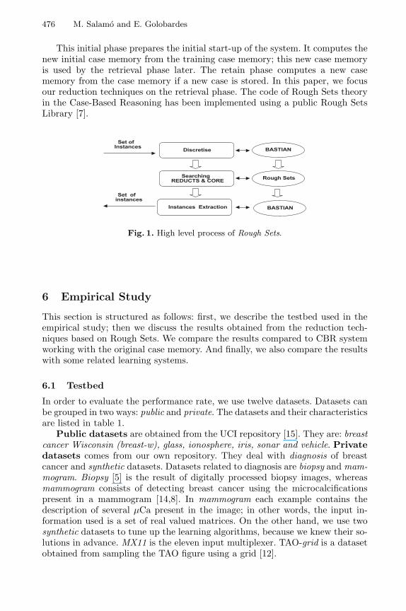
Figure 1 shows the meta-level process when incorporating the Rough Sets intothe CBR system. The Rough Sets process is divided into three steps:

The first one discretises the instances, it is necessary to find the most relevantinformation using the Rough Sets theory. In that case, we discretise continuousfeatures using [4] algorithm. The second step searches for the reducts and thecore of knowledge using the Rough Sets theory, as was described in section 4.Finally, the third step uses the core and the reducts of knowledge to decidewhich cases are maintained in the case memory using AccurCM and ClassCMtechniques, as explained in 4.2.

Rough Sets theory has been introduced as reduction techniques in two phasesof the CBR cycle. The first phase is the start-up phase and the second one isthe retain phase. The system adds a previous phase Startup, which is not in theCase-Based Reasoning cycle.

476 M. Salamo and E. Golobardes

This initial phase prepares the initial start-up of the system. It computes thenew initial case memory from the training case memory; this new case memoryis used by the retrieval phase later. The retain phase computes a new casememory from the case memory if a new case is stored. In this paper, we focusour reduction techniques on the retrieval phase. The code of Rough Sets theoryin the Case-Based Reasoning has been implemented using a public Rough SetsLibrary [7].

Set ofInstances

Discretise BASTIAN

Rough SetsSearchingREDUCTS & CORE

Instances Extraction BASTIAN

Set ofinstances

Fig. 1. High level process of Rough Sets.

6 Empirical Study

This section is structured as follows: first, we describe the testbed used in theempirical study; then we discuss the results obtained from the reduction tech-niques based on Rough Sets. We compare the results compared to CBR systemworking with the original case memory. And finally, we also compare the resultswith some related learning systems.

6.1 Testbed

In order to evaluate the performance rate, we use twelve datasets. Datasets canbe grouped in two ways: public and private. The datasets and their characteristicsare listed in table 1.

Public datasets are obtained from the UCI repository [15]. They are: breastcancer Wisconsin (breast-w), glass, ionosphere, iris, sonar and vehicle. Privatedatasets comes from our own repository. They deal with diagnosis of breastcancer and synthetic datasets. Datasets related to diagnosis are biopsy and mam-mogram. Biopsy [5] is the result of digitally processed biopsy images, whereasmammogram consists of detecting breast cancer using the microcalcificationspresent in a mammogram [14,8]. In mammogram each example contains thedescription of several µCa present in the image; in other words, the input in-formation used is a set of real valued matrices. On the other hand, we use twosynthetic datasets to tune up the learning algorithms, because we knew their so-lutions in advance. MX11 is the eleven input multiplexer. TAO-grid is a datasetobtained from sampling the TAO figure using a grid [12].

Rough Sets Reduction Techniques for Case-Based Reasoning 477

These datasets were chosen in order to provide a wide variety of applicationareas, sizes, combinations of feature types, and difficulty as measured by theaccuracy achieved on them by current algorithms. The choice was also madewith the goal of having enough data points to extract conclusions.

All systems were run using the same parameters for all datasets. The per-centage of correct classifications has been averaged over stratified ten-fold cross-validation runs, with their corresponding standard deviations. To study the per-formance we use paired t-test on these runs.

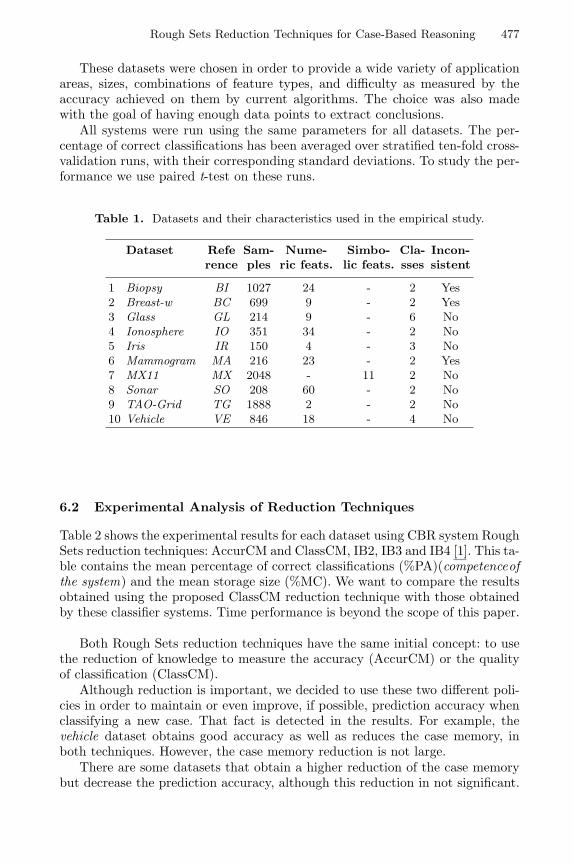
Table 1. Datasets and their characteristics used in the empirical study.

Dataset Refe Sam- Nume- Simbo- Cla- Incon-rence ples ric feats. lic feats. sses sistent

1 Biopsy BI 1027 24 - 2 Yes2 Breast-w BC 699 9 - 2 Yes3 Glass GL 214 9 - 6 No4 Ionosphere IO 351 34 - 2 No5 Iris IR 150 4 - 3 No6 Mammogram MA 216 23 - 2 Yes7 MX11 MX 2048 - 11 2 No8 Sonar SO 208 60 - 2 No9 TAO-Grid TG 1888 2 - 2 No10 Vehicle VE 846 18 - 4 No

6.2 Experimental Analysis of Reduction Techniques

Table 2 shows the experimental results for each dataset using CBR system RoughSets reduction techniques: AccurCM and ClassCM, IB2, IB3 and IB4 [1]. This ta-ble contains the mean percentage of correct classifications (%PA)(competenceofthe system) and the mean storage size (%MC). We want to compare the resultsobtained using the proposed ClassCM reduction technique with those obtainedby these classifier systems. Time performance is beyond the scope of this paper.

Both Rough Sets reduction techniques have the same initial concept: to usethe reduction of knowledge to measure the accuracy (AccurCM) or the qualityof classification (ClassCM).

Although reduction is important, we decided to use these two different poli-cies in order to maintain or even improve, if possible, prediction accuracy whenclassifying a new case. That fact is detected in the results. For example, thevehicle dataset obtains good accuracy as well as reduces the case memory, inboth techniques. However, the case memory reduction is not large.

There are some datasets that obtain a higher reduction of the case memorybut decrease the prediction accuracy, although this reduction in not significant.

478 M. Salamo and E. Golobardes

Table 2. Mean percentage of correct classifications and mean storage size. Two-sidedpaired t-test (p = 0.1) is performed, where a • and ◦ stand for a significant improvementor degradation of our ClassCM approach related to the system compared. Bold fontindicates the best prediction accuracy.

Ref. CBR AccurCM ClassCM IB2 IB3 IB4

BIBCGLIOIRMAMXSOTGVE

%PA %CM83.15 100.096.28 100.072.42 100.090.59 100.096.0 100.064.81 100.078.61 100.084.61 100.095.76 100.067.37 100.0

%PA %CM75.15• 2.7594.56 58.7658.60• 23.8888.60• 38.9894.00◦ 96.5066.34◦ 81.5668.00• 0.5475.48• 33.0196.34◦ 95.3964.18• 34.75

%PA %CM84.41 1.7396.42 43.9571.12 76.1192.59 61.0087.40 8.8559.34 37.5078.74 99.9086.05 67.0586.97 13.1468.42 65.23

%PA %CM75.77• 26.6591.86• 8.1862.53• 42.9986.61• 15.8293.98◦ 9.8566.19 42.2887.07◦ 18.9980.72 27.3094.87◦ 7.3865.46• 40.01

%PA %CM78.51• 13.6294.98 2.8665.56• 44.3490.62 13.8991.33 11.2660.16 14.3081.59 15.7662.11• 22.7095.04◦ 5.6363.21• 33.36

%PA %CM76.46• 12.8294.86 2.6566.40• 39.4090.35 15.4496.66 12.0060.03 21.5581.34 15.8463.06• 22.9293.96◦ 5.7963.68• 31.66

Comparing AccurCM and ClassCM, the most regular behaviour is achievedusing ClassCM. This behaviour is due to its own nature, because it introducesall the border cases classifying the class correctly into the reduced case memory,as well as the internal cases needed to complete all classes. AccurCM calculatesthe border points of the case memory. AccurCM calculates the degree of com-pleteness of our knowledge, which can be seen as the coverage [25]. AccurCMpoints out the relevance of classification of each case.

ClassMC reduction technique obtains on average a higher generalisation ac-curacy than IBL, as can be seen in table 2. There are some datasets whereClassCM shows a significant increase in the prediction accuracy. The perfor-mance of IBL algorithms declines when case memory is reduced. CBR obtainson average higher prediction accuracy than IB2, IB3 and IB4.

On the other hand, the mean storage size obtained for ClassCM is higherthan that obtained when using IBL schemes (see table 2). IBL algorithms obtaina higher reduction of the case memory. However, IBL performance declines,in almost all datasets (e.g. Breast-w, Biopsy). This degradation is significantin some datasets, as happens with the sonar dataset. Our initial purpose forthe reduction techniques was to reduce the case memory as much as possible,maintaining the generalisation accuracy. We should continue working to obtaina higher reduction on the case memory.

To finish the empirical study, we also run additional well-known reductionschemes on the previous data sets. The reduction algorithms are: CNN, SNN,DEL, ENN, RENN, DROP1, DROP2, DROP3, DROP4 and DROP5 (a completeexplanation of them can be found in [26]). We use the same data sets describedabove but with different ten-fold cross validation sets. We want to compare theresults obtained using the proposed ClassCM reduction technique with thoseobtained by these reduction techniques. Tables 3 and 4 show the mean predictionaccuracy and the mean storage size for all systems in all datasets, respectively.

Table 3 shows the behaviour of our ClassCM reduction technique in com-parison with CNN, SNN, DEL, ENN and RENN techniques. The results are onaverage better than those obtained by the reduction techniques studied. RENN

Rough Sets Reduction Techniques for Case-Based Reasoning 479

Table 3. Mean percentage of correct classifications and mean storage size. Two-sidedpaired t-test (p = 0.1) is performed, where a • and ◦ stand for a significant improvementor degradation of our ClassCM approach related to the system compared. Bold fontindicates the best prediction accuracy.

Ref. ClassCM CNN SNN DEL ENN RENN

BIBCGLIOIRMAMXSOTGVE

%PA %CM84.41 1.7396.42 43.9571.12 76.1192.59 61.0087.40 8.8559.34 37.5078.74 99.9086.05 67.0586.97 13.1468.42 65.23

%PA %CM79.57• 17.8295.57 5.8767.64 24.9788.89• 9.9496.00◦ 14.0061.04 25.0689.01◦ 37.1783.26 23.4594.39◦ 7.1569.74 23.30

%PA %CM78.41• 14.5195.42 3.7267.73 20.5185.75• 7.0094.00◦ 9.9363.42◦ 18.0589.01◦ 37.1580.38 20.5294.76◦ 6.3869.27 19.90

%PA %CM82.79• 0.3596.57◦ 0.3264.87• 4.4780.34• 1.0196.00◦ 2.5262.53◦ 1.0368.99• 0.5577.45• 1.1287.66 0.2662.29• 2.55

%PA %CM77.82• 16.5295.28 3.6168.23 19.3288.31• 7.7991.33 8.5963.85◦ 21.6685.05◦ 32.5485.62 19.3496.77◦ 3.7566.91 20.70

%PA %CM81.03• 84.5197.00◦ 96.3468.66 72.9085.18• 86.3996.00◦ 94.4465.32◦ 66.9299.80◦ 99.8982.74 86.4995.18◦ 96.5168.67 74.56

improves the results of ClassCM in some data sets (e.g. Breast-w) but its reduc-tion on the case memory is lower than ClassCM.

Table 4. Mean percentage of correct classifications and mean storage size. Two-sidedpaired t-test (p = 0.1) is performed, where a • and ◦ stand for a significant improvementor degradation of our ClassCM approach related to the system compared. Bold fontindicates best prediction accuracy.

Ref. ClassCM DROP1 DROP2 DROP3 DROP4 DROP5

BIBCGLIOIRMAMXSOTGVE

%PA %CM84.41 1.7396.42 43.9571.12 76.1192.59 61.0087.40 8.8559.34 37.5078.74 99.9086.05 67.0586.97 13.1468.42 65.23

%PA %CM76.36• 26.8493.28 8.7966.39 40.8681.20• 23.0491.33 12.4461.60 42.6987.94◦ 19.0284.64 25.0594.76◦ 8.0364.66• 38.69

%PA %CM76.95• 29.3892.56 8.3569.57 42.9487.73• 19.2190.00 14.0758.33 51.34100.00◦ 98.3787.07 28.2695.23◦ 8.9567.16 43.21

%PA %CM77.34• 15.1696.28 2.7067.27 33.2888.89 14.2492.66 12.0758.51 12.6082.37 17.1076.57• 16.9394.49◦ 6.7666.21 29.42

%PA %CM76.16• 28.1195.00 4.3769.18 43.3088.02• 15.8388.67 7.9358.29 50.7786.52 25.4784.64 26.8289.41◦ 2.1868.21 43.85

%PA %CM76.17• 27.0393.28 8.7965.02• 40.6581.20• 23.0491.33 12.4461.60 42.6486.52 18.8984.64 25.1194.76◦ 8.0364.66• 38.69

In table 4 the results obtained using ClassCM and DROP algorithms arecompared. ClassCM shows better competence for some data sets (e.g. biopsy,breast-w, glass), although its results are also worse in others (e.g. multiplexer).The behaviour of these reduction techniques are similar to the previously stud-ied. ClassCM obtains a balance behaviour between competence and size. Thereare some reduction techniques that obtain best competence for some data setsreducing less the case memory size.

All the experiments (tables 2, 3 and 4) point to some interesting observa-tions. First, it is worth noting that the individual AccurCM and ClassCM workswell in all data sets, obtaining better results on ClassCM because the reductionis smaller. Second, the mean storage obtained using AccurCM and ClassCMsuggest complementary behaviour. This effect can be seen on the tao-grid data

480 M. Salamo and E. Golobardes

set, where AccurCM obtains a 95.39% mean storage and ClassCM 13.14%. Wewant to remember that ClassCM complete the case memory in order to obtainat least one case of each class. This complementary behaviour suggests that theycan be used together in order to improve the competence and maximise the re-duction of the case memory. Finally, the results on all tables suggest that allthe reduction techniques work well in some, but not all, domains. This has beentermed the selective superiority problem [2]. Consequently, future work consistsof combining both approaches in order to exploit the strength of each one.

7 Conclusions and Further Work

This paper introduces two new reduction techniques based on the Rough Setstheory. Both reduction techniques have a different nature: AccurCM reduces thecase memory maintaining the internal cases; and ClassCM obtains a reducedset of border cases, increasing that set of cases with the most relevant classifiercases. Empirical studies show that these reduction techniques produce a higheror equal generalisation accuracy on classification tasks. We conclude that RoughSets reduction techniques should be improved in some ways. That fact focus ourfurther work. First, the algorithm selectCases should be changed in order toselect a most reduced set of cases. In this way, we want to modifiy the algorithmselecting only the most representative K-nearest neighbour cases that accom-plishing the confidenceLevel. Second, we should search for new discretisationmethods in order to improve the pre-processing of the data. Finally, we want toanalyse the influence of the weighting methods in these reduction techniques.

Acknowledgements. This work is supported by the Ministerio de Sanidady Consumo, Instituto de Salud Carlos III, Fondo de Investigacion Sanitaria ofSpain, Grant No. 00/0033-02. The results of this study have been obtained us-ing the equipment co-funded by the Direccio de Recerca de la Generalitat deCatalunya (D.O.G.C 30/12/1997). We wish to thank Enginyeria i ArquitecturaLa Salle (Ramon Llull University) for their support of our Research Group inIntelligent Systems. We also wish to thank: D. Aha for providing the IBL codeand D. Randall Wilson and Tony R. Martinez who provided the code of theother reduction techniques. Finally, we wish to thank the anonymous reviewersfor their useful comments during the preparation of this paper.

References

1. D. Aha and D. Kibler. Instance-based learning algorithms. Machine Learning,Vol. 6, pages 37–66, 1991.

2. C.E. Brodley. Addressing the selective superiority problem: Automatic algo-rithm/model class selection. In Proceedings of the 10th International Conferenceon Machine Learning, pages 17–24, 1993.

3. P. Domingos. Context-sensitive feature selection for lazy learners. In AI Review,volume 11, pages 227–253, 1997.

Rough Sets Reduction Techniques for Case-Based Reasoning 481

4. U.M. Fayyad and K.B. Irani. Multi-interval discretization of continuous-valuedattributes for classification learning. In 19th International Joint Conference onArtificial Intelligence, pages 1022–1027, 1993.

5. J.M. Garrell, E. Golobardes, E. Bernado, and X. Llora. Automatic diagnosis withGenetic Algorithms and Case-Based Reasoning. Elsevier Science Ltd. ISSN 0954-1810, 13:367–362, 1999.

6. G.W. Gates. The reduced nearest neighbor rule. In IEEE Transactions on Infor-mation Theory, volume 18(3), pages 431–433, 1972.

7. M. Gawry’s and J. Sienkiewicz. Rough Set Library user’s Manual. Technical Report00-665, Computer Science Institute, Warsaw University of Technology, 1993.

8. E. Golobardes, X. Llora, M. Salamo, and J. Martı. Computer Aided Diagnosiswith Case-Based Reasoning and Genetic Algorithms. Knowledge Based Systems(In Press), 2001.

9. P.E. Hart. The condensed nearest neighbour rule. IEEE Transactions on Infor-mation Theory, 14:515–516, 1968.

10. J. Kolodner. Case-Based Reasoning. Morgan Kaufmann Publishers, Inc., 1993.11. D. Leake and D. Wilson. Remembering Why to Remember:Performance-Guided

Case-Base Maintenance. In Proceedings of the Fifth European Workshop on Case-Based Reasoning, 2000.

12. X. Llora and J.M. Garrell. Inducing partially-defined instances with Evolution-ary Algorithms. In Proceedings of the 18th International Conference on MachineLearning (To Appear), 2001.

13. D.G. Lowe. Similarity Metric Learning for a Variable-Kernel Classifier. In NeuralComputation, volume 7(1), pages 72–85, 1995.

14. J. Martı, J. Espanol, E. Golobardes, J. Freixenet, R. Garcıa, and M. Salamo. Clas-sification of microcalcifications in digital mammograms using case-based reasonig.In International Workshop on digital Mammography, 2000.

15. C. J. Merz and P. M. Murphy. UCI Repository for Machine Learning Data-Bases[http://www.ics.uci.edu/∼mlearn/MLRepository.html]. Irvine, CA: University ofCalifornia, Department of Information and Computer Science, 1998.

16. Z. Pawlak. Rough Sets. In International Journal of Information and ComputerScience, volume 11, 1982.

17. Z. Pawlak. Rough Sets: Theoretical Aspects of Reasoning about Data. KluwerAcademic Publishers, 1991.

18. L. Portinale, P. Torasso, and P. Tavano. Speed-up, quality and competence inmulti-modal reasoning. In Proceedings of the Third International Conference onCase-Based Reasoning, pages 303–317, 1999.

19. C.K. Riesbeck and R.C. Schank. Inside Case-Based Reasoning. Lawrence ErlbaumAssociates, Hillsdale, NJ, US, 1989.

20. G.L. Ritter, H.B. Woodruff, S.R. Lowry, and T.L. Isenhour. An algorithm fora selective nearest neighbor decision rule. In IEEE Transactions on InformationTheory, volume 21(6), pages 665–669, 1975.

21. M. Salamo and E. Golobardes. BASTIAN: Incorporating the Rough Sets theoryinto a Case-Based Classifier System. In III Congres Catala d’Intel·ligencia Artifi-cial, pages 284–293, October 2000.

22. M. Salamo, E. Golobardes, D. Vernet, and M. Nieto. Weighting methods for aCase-Based Classifier System. In LEARNING’00, Madrid, Spain, 2000. IEEE.

23. S. Salzberg. A nearest hyperrectangle learning method. Machine Learning, 6:277–309, 1991.

482 M. Salamo and E. Golobardes

24. B. Smyth and M. Keane. Remembering to forget: A competence-preserving casedeletion policy for case-based reasoning systems. In Proceedings of the ThirteenInternational Joint Conference on Artificial Intelligence, pages 377–382, 1995.

25. B. Smyth and E. McKenna. Building compact competent case-bases. In Proceedingsof the Third International Conference on Case-Based Reasoning, 1999.

26. D.R. Wilson and T.R. Martinez. Reduction techniques for Instance-Based LearningAlgorithms. Machine Learning, 38, pages 257–286, 2000.

27. Q. Yang and J. Wu. Keep it Simple: A Case-Base Maintenance Policy Based onClustering and Information Theory. In Proc. of the Canadian AI Conference, 2000.

28. J. Zhu and Q. Yang. Remembering to add: Competence-preserving case-additionpolicies for case base maintenance. In Proceedings of the Fifteenth InternationalJoint Conference on Artificial Intelligence, 1999.