Classification and rule induction using rough set theory

ArticleClassification and ruleinduction using rough settheory

Malcolm Beynon, Bruce Curryand Peter Morgan

Cardiff Business School, Cardiff University,Colum Drive, Cardiff CF10 3EU, UKE-mail: beynonMJKcardiff.ac.uk

Abstract: Rough set theory (RST) offers an interestingand novel approach both to the generation of rules foruse in expert systems and to the traditional statisticaltask of classification. The method is based on a novelclassification metric, implemented as upper and lowerapproximations of a set and more generally in terms ofpositive, negative and boundary regions. Classificationaccuracy, which may be set by the decision maker, ismeasured in terms of conditional probabilities forequivalence classes, and the method involves a searchfor subsets of attributes (called ‘reducts’) which do notrequire a loss of classification quality. To illustrate thetechnique, RST is employed within a state levelcomparison of education expenditure in the USA.

Keywords: rough sets, classification, decision tables,rule induction, set approximation

1. Introduction

Rough set theory (RST) offers an interesting and novelapproach both to the generation of rules for use in expertsystems and to the traditional statistical task of classi-fication. Its philosophy is founded on the assumption thatwith every object of the universe of discourse there is someassociated information, data or knowledge (Krawiecet al.,1998). Recent papers have looked at RST with respect toother modern techniques of data analysis including evi-dence theory (Skowron & Grzymala-Busse, 1994). More-

136 Expert Systems, July 2000, Vol. 17, No. 3

over, comparisons have been made with other methods suchas discriminant analysis (Krusinskaet al., 1992; Browneet al., 1998; Dimitras et al., 1999), logistic analysis(Dimitraset al., 1999) and neural networks (Jeloneket al.,1995; Szczuka, 1998).

Pawlaket al. (1995) discuss the application of RST tothe reduction of data for a neural network, finding thatlearning time accelerates data reduction by up to 4.72 times,hence exhibiting a useful tool for preprocessing of data forneural networks. Pawlak (1998, p. V) concludes that

RST lies on the crossroads of fuzzy sets, theory of evidence, neuralnetworks, Petri nets and many other branches of artificial intelligence,logic and mathematics.

However, rather than being a technique for automated ruleinduction, RST requires a level of input from a decisionmaker, and so is not as yet suitable as a means ofimplementing machine learning. It can of course also beargued that rule generation is a statistical task, and therelationships between RST and mainstream statisticalreasoning are discussed in this paper. We may usefully stateat the outset, however, that RST may to some readersappear to be almost ‘anti-statistical’ in nature!

In what follows we outline the basic principles behindthe original concepts of RST and proceed to consider thevariable precision rough set (VPRS) model, a more recentgeneralization which incorporates probabilities. We thenoutline procedures generating rules suitable for the purposeof classification. These concepts are further illustratedthrough an example, in this case a US state by state com-parison of the expenditure per student in elementary andsecondary schools based on proportions of stated ethnicitylevels of students. The VPRS analysis of the example pro-duces rules which individually classify groups of states.These rules may subsequently be used to provide predic-tions of expenditure for a ‘holdout’ sample of states. Theexample illustrates the novel results of analysis in whatwould be considered a ‘small data’ set. Indeed, Getis (1999)considers that we should be uncomfortable with 50 statesplus the District of Columbia as a basis for conventionalanalysis. To provide comparisons with our results a lineardiscriminant analysis model is also presented for thesame data.

2. Basic concepts

RST has its origins in pure mathematics (Pawlak, 1982)and, as presented below, has a rigorous theoretical foun-dation. As can be seen from the names of the relevantauthors working in this area, the Polish influence has beenprominent in its development. The nascent research interest

in rough sets can be gauged through the number of researcharticles produced — by 1991 there had been over 400 art-icles and reports published on RST and its applications(Pawlak, 1991). By 1993 there were over 800 publicationsin this area, including two books and an annual workshop(Ziarko, 1993a).

RST operates on what may be described as a decisiontable or ‘information system’. In statistical terminology thiswould be described as a data matrix or data table. As canbe seen in the example in Table 1, we have a set of objectsU (o1, . . ., o7) contained in the rows of the table, with thecolumns denoting condition attributesC (c1, . . ., c6) ofthese objects and a related decision attributeD (d1), a valuedenoting the nature of an attribute to an object and calleda ‘descriptor’. To use RST one must have data in discreteor categorical form. A range of discretization procedures isavailable, such as the minimal class entropy method(Fayyad & Irani, 1992) and the global discretization methodof Chmielewski and Grzymala-Busse (1996), which isbased on median clustering.

In this particular decision table the condition attributedescriptors are made up of 1s and 0s (e.g. yes/no answers)and the decision attributes are ‘M’ or ‘F’ (e.g. Male orFemale). One may criticize authors writing on RST for theoften confusing terminology and notation that is employedand that has become standard. In our view it is useful tofocus initially on the theme of classification. In Table 1 wehave the information that objects have been classified intoone of two categories (decisions), M and F, also describedas ‘concepts’.

Fundamental to RST is the classification of data points(‘objects’ in RST terminology) which are ideal in the senseof being completely unambiguous. An unambiguous classi-fication has the property that objects with identical sets ofattributes should belong to the same decision category. RSTprovides measures of the extent to which this ideal isattained. The measures are based entirely on the availableset of data. Taking the data in this way at face value runscounter to the standard approach to statistical inferencewhereby sampling aspects are prominent.

In the example in Table 1, objectso1, o3, o4 ando6 areunambiguouslyclassified, in the sense that all objects with

Table 1: Decision table

Objects c1 c2 c3 c4 c5 c6 d1

o1 1 1 1 1 1 1 Mo2 1 0 1 0 1 1 Mo3 0 0 1 1 0 0 Mo4 1 1 1 0 0 1 Fo5 1 0 1 0 1 1 Fo6 0 0 0 1 1 0 Fo7 1 0 1 0 1 1 F

Expert Systems, July 2000, Vol. 17, No. 3 137

a given set of attribute values are assigned to the samedecision category. Also of interest are objects which maypossiblybe classified to a certain category, in the sense thatnot all objects with a given set of attribute values belongto the same category. Thus, objectso2, o5 and o7 areambiguouslyclassified. The set of objects which are defi-nitely (i.e. unambiguously) classified is known as the‘lower approximation’, and the set of objects possibly ordefinitely classified is the ‘upper approximation’.

RST in its original form is based on the simple andelegant principle that for each decision category wemeasure the effectiveness of classification by comparingthe number of objects definitely classified to that cate-gory with the numbers possibly or definitely classified.The ratio for each category is known as the ‘accuracy ofapproximation’, and for the data set as a whole the ‘qual-ity of approximation’.

3. A formal treatment

We denote byC andD respectively the condition attributesand decision values, withA denoting the set of conditionand decision attribute values taken together, i.e.A = C <D. For formal analysis, and also for computational pur-poses, we need to focus on objects which are identical inevery respect. We therefore define an indiscernibilityrelation as a binary relation IND(P), defined for some sub-setP of A (P # A).

IND(P) = h(x, y) P U2: for everya P P, a(x) = a(y)j

Subsequently, we define theequivalence classesof objectsfor the condition attributes as groupings of indiscernibleobjects, in which case, for our example, we have the equiv-alence classes (for condition attributes) as

X1 = ho1j X2 = ho2, o5, o7jX3 = ho3j X4 = ho4j X5 = ho6j

Similarly, the equivalence classes of the decision categor-ies are

YM = ho1, o2, o3j YF = ho4, o5, o6, o7j

In equivalence classX2, for example, the objects are ident-ical in their condition attribute values, although not for thedecision categories they belong to. The lower and upperapproximations are then formally defined as follows:

P-lower approximation= PZ = hE(P): E(P) # Zj

P-upper approximation= PZ = hE(P): E(P) > Z Þ [}

for Z # U, the ‘universe’ of objects. We also define theboundary regionBNP(Z) as the difference between these

sets, i.e. the objects possibly classified. These definitions,and hence also the computations, operate on the equival-ence classes. To illustrate letP = hc1, c2, c3j and Z = ho5,o6j. The equivalence classes (Eis) of P are then

E1 = ho1, o4j E2 = ho2, o5, o7j E3 = ho3j E4 = ho6j

Of these onlyE4 is contained entirely inZ, in which casePZ = ho6j. For the upper approximation we consider non-empty intersections of theEis with Z. It follows thatE2 andE4 are then the relevant equivalence classes, givingPZ =E2 < E4 = ho2, o5, o6, o7j and thereforeBNP(Z) = ho2, o5,o7j. Using P = hc1, c2, c3j, only two objects overall haveunambiguous classification: these are objectso3 ando6. Thequality of approximation is then 2/7. Working with thecomplete set of attributes (P = C), four out of seven objects(quality of approximation) are unambiguously classified:these areX1, X3, X4 and X5. The use of all attributes hasthe effect of making fewer objects indiscernible, i.e.increasing the number of equivalence classes.

The definition of the lower approximation of a setinvolves an inclusion relation whereby the objects in anequivalence class of the attributes are entirely contained inthe equivalence class for a decision category. This is thecase of perfect or unambiguous classification. For the upperapproximation we take the union of intersections: the defi-nition operates with all equivalence classes of the attributeswhich have a non-empty intersection with a decision class.We are then using all objects which may be classified.Figure 1 gives an illustration of these ideas by means of adiagrammatic method due to Bjorvand (1996).

In Figure 1 the squares represent the equivalence classesof the information system with respect to a subset of attri-butes, sayP (with P # C). The area enclosed by the free-hand drawing isZ (a subset of objects). TheP-lowerapproximation is then the dark grey squares, i.e. thoseequivalence classes comprising objects fully contained inZ. The P-upper approximation is depicted by the dark andthe light grey squares. TheBNP(Z) region is depicted bythe light grey squares.

Figure 1: Visual interpretation of rough sets.


4. The VPRS model: generalization for partialclassifications

The VPRS model originally suggested by Ziarko (1993b,1993c) provides a powerful generalization of RST. Thegeneralization is such that we are no longer restricted toobjects which are certainly classified to categories and caninstead handle conditional probabilities. The latter aredefined for equivalence classes, so that for equivalenceclassX2 = ho2, o5, o7j for example, relating to the full setof attributes, objectso5 ando7 are assigned to categoryYF

and we have the conditional probability Pr(YF u X2) = 2/3.This concentration on subsets of objects defined in terms

of equivalence classes implies a rather different emphasisfor RST compared with conventional statistical methods.The latter relate to particular data points, to the entire dataset or to subsets defined in a certain way, e.g. temporally.VPRS deals with partial classification by introducing aprobability valueb (using the definition due to Anet al.(1996)), which has some similarities with the level of sig-nificance used in conventional statistical methods. For anyequivalence class groups of objects may be classified todifferent decision categories. The value ofb measures thesize of the largest group (of objects) as a proportion of thetotal number of objects in the equivalence class. It may beviewed as a conditional probability, namely the probabilityof a decision category given a specified equivalence class.

What we term ‘original’ RST amounts to the special caseb = 1, but in VPRS we now permit a range of values,bounded below byb = 0.5. For any value ofb, we mayidentify the equivalence classes which have the propertythat thelargest proportionof objects classified to the samecategory is at leastb. Also of interest is the proportion ofthose objects definitely not classified: this must not exceed1 − b. The sets are known respectively as theb-positiveand b-negative regions and the difference between thesetwo sets, which is crucial to the rule generation process, isreferred to as theb-boundary region.

Formal definitions of the set approximations are then

b-positive region of the setZ # U and P # C:POSb

P(Z) = <Pr(ZuXi)$b hXi P E(P)jb-negative region of the setZ # U andP # C:

NEGbP(Z) = <Pr(ZuXi)#1 − b hXi P E(P)j

b-boundary region of the setZ # U and P # C:BNDb

P(Z) = <1 − b,Pr(ZuXi),b hXi P E(P)j

The use of probabilities in these definitions corresponds tothe use of ‘majority inclusion’ relations for classification.In the example, using the defined subset of attributesP =hc1, c2, c3j, with b = 0.8 and using againZ = ho5, o6j

POSbP(Z) = ho6j NEGb

P(Z) = ho1, o3, o4j

BNDbP(Z) = ho2, o5, o7j

This is because, atb = 0.8, objecto6 is fully included inZ and objectsho1, o3, o4j are fully excluded fromZ. Thevalue ofb is too strict for unambiguous classification ofho2,o5, o7j. However, lettingb fall to 0.6, since the conditionalprobability of non-inclusion inZ for the latter is 2/3, theequivalence classho2, o5, o7j moves into theb-negativeregion and the boundary region becomes empty.

We may envisage, in general, starting atb = 1, at whichpoint POSbP(Z) coincides with theP-lower approximationPZ, and thence progressively lowering the value ofb untilthe boundary region becomes the empty set or we reachthe boundary pointb = 0.5. An empty boundary regionmeans that each object is given a classification. We seekan empty boundary region for as high a value ofb as poss-ible, in the same sense that in significance testing we canoperate by finding the best significance level at which thenull hypothesis can still be rejected. Alternatively, as withsignificance tests, we may specify a value ofb, reflectingthe judgement of the decision maker. These issues are dis-cussed further below.

In formal terms, we are working not with an inclusionrelation as above but with a novel concept, due to Ziarko(1993b), of majority inclusion. We have a proportionb ofobjects in an equivalence class included in a set denotinga decision category: this proportion is specified, perhapsarbitrarily, to amount at least to a majority (at least greaterthan 50% of objects in the equivalence class). Thus in theexample, using Ziarko’s notation, we may make statements

such asX2 #b

YF for any b P (0.5, 0.667].1

4. 1. Reducing the number of attributes

Having defined and computed measures relating to thequality or ambiguity of classification, we also seek to achievea given level of quality by using only subsets of attributes.We may seek a minimal set of attributes. Equally, andthis is where RST provides an emphasis rather differentfrom more conventional statistical methods, we may wishto generate rules applying only to certain subsets of objectsspecified by the decision maker. In original RST, thismeans defining a ‘reduct’ which has the property that thesame measured quality of approximation may be achieveddespite removal of certain attributes. Interestingly, Pawlaket al. (1995) claim (from a study involving a neural networkwith a single hidden layer) that the minimum number ofneurons in the hidden layer is equal to the cardinality of thesmallest reduct. In VPRS, we need a generalized version ofthis measure of quality.

Ziarko (1993b) defines

gb(P, D) =card[<Pr(ZuXi)$bhXi P E(P)j]

card(U)

1The range 0.5 (not including 0.5) up to and including 0.667.


whereZ P E(D), P P C, for a specified value ofb. Thevalue gb(P, D) measures the proportion of objects in theuniverse (or complete data set) for which classification ispossible at the specified value ofb. In other words, itinvolves combining allb-positive regions and working withthe number of objects involved in such a combination. Inthe example in Table 1, working with the full set of attri-butes and commencing withb = 1, objectso1 ando2 maybe unambiguously classified to category M and objectso4

ando6 unambiguously to category F. The value ofgb(P, D)is then 4/7. If we allowb to fall to 0.6 (i.e. less than orequal to 0.667), then we obtain a value of unity for themeasure, i.e.gb(C, D) = 1 for b P (0.5, 0.667].

In VPRS we consider a probabilistic reduct REDb(C, D),referred to as ab-reduct, which has the twin properties that

(1) gb(C, D) = gb(REDb(C, D), D);(2) no attribute can be eliminated from REDb(C, D) with-

out affecting the requirement (1).

It is important to note that ab-reduct may consist of anumber of equivalence classes, for each one of which theremay exist a thresholdb value where the boundary regionis empty (Ziarko, 1993b); otherwise the equivalence classis not given a classification. Considering theb-reduct as awhole, we define the valuebmin to be the minimum valueof these thresholds, i.e. the worst case value. Table 2 showsfour b-reducts (for which quality of approximation is unity)for the decision table in Table 1.

In VPRS, by convention, only reducts with abmin valueexceeding 0.5 are considered. Above this value the decisionmaker may impose a threshold, in the same way as onemay select levels of significance for statistical tests.

4. 2. Rule generation

Rules are generated fromb-reducts. Anet al. (1996) sug-gest a procedure whereby rules are extracted fromb-reducts on the basis of attribute descriptors. Each equival-ence class in theb-reduct generates a rule and the certaintyfactor for a rule follows from the conditional probabilitytherein. To illustrate this, Table 3 gives the minimum setof rules for two of the aboveb-reducts, namelyb-reduct 3hc3, c6j andb-reduct 4hc2, c5j.

Each row in these tables relates to the equivalenceclasses for the respective reducts. The final columns in

Table 2: b-reducts associated with decision table inTable 1

b-reduct 1 bmin b-reduct 2 bmin

hc1, c3j 0.60 hc4j 0.66

b-reduct 3 bmin b-reduct 4 bmin

hc3, c6j 0.60 hc2, c5j 0.75

Table 3, labelledS andP respectively, indicate the qualityaspects of the rules.Sshows the number of objects involvedandP the proportion (conditional probability) allocated orcategorized by the rule. Thus, for example, rule 3 forb-reduct 4hc2, c5j involves four objects, of which three arecorrectly classified. The values of the attributes are ‘0’ and‘1’ respectively, and the decision category is F. Theimportant point to be made here is that the rule is generatedautomatically by a simple reading of attribute values.Whether the classification error (bmin value) is acceptableis a matter of choice for the decision maker.

4. 3. Reduct selection

Reduct selection may be on the grounds of thebmin value,and hence requires the judgement of the decision maker.Reduct selection can be on the basis of the smallest numberof attributes or the maximum number of objects classified(Wakulicz-Deja & Paszek, 1997), or of the increase in thequality of classification by successive augmentation of thesubset of attributes (Moraczewskiet al., 1996; Slowinskiet al., 1997), through to the use of an expert (Dimitraset al., 1999). Selection can also be on the basis of the rel-evance of the rules to the decision. This has to be a matterentirely of judgement. An alternative approach is to assigna cost or importance function to the attributes, perhaps inconjunction with domain experts.

5. An illustrative application

In this section we consider as an example the analysis ofexpenditure on elementary and secondary school educationat the US state level, part of a more extensive on-goingproject. One aspect of this analysis is the small data setinvolved, i.e. the 50 states of America plus the District ofColumbia (DC). The data employed for this exercise are

Table 3: Rules generated forb-reduct 3 hc3, c6j andb-reduct 4hc2, c5j

Rule c3 c6 d1 S P

1 If 1 and 0 then M 1 12 If 1 then F 5 0.603 If 0 then F 1 1

c2 c5

1 If 1 and 1 then M 1 12 If 0 and 0 then M 1 13 If 0 and 1 then F 4 0.754 If 1 and 0 then F 1 1


all obtained from the US Government’s National Centre ofEducational Statistics.2

The scatter plot diagram given in Figure 2 (top) showsthe positions of the states (using standard postcode abbrevi-ations, e.g. AL, Alabama) based on expenditure per studentagainst average number of students per school. While astrong positive correlation exists (R = 0.809, significant atthe 0.01 level) between these factors, there are variations.For example, while AL and AK have similar levels ofexpenditure, their average numbers of students per schoollevels are quite different. Since any decision variable (aswith condition attributes) needs to be in categorical form,we employed a cluster analysis to group the states into threecategories. These are also shown in the scatter plot in Fig-ure 2. Specifically, we have used thek-means clusteringoption in SPSS (version 9), applying the Euclidean distancemetric. To further illustrate the results, Figure 2 (bottom)also shows the clustering of the states (geographically) on amap of the USA. We note in passing that certain interestingpatterns emerge, such as the majority of states in Cluster 1grouped (geographically) together in the northeast of theUSA and the bisection of Cluster 3 by Cluster 2. Furtherinterpretation is not included in this paper.

To illustrate the rule classification and predictive oppor-tunities of VPRS, the 51 states are split into an ‘in sample’of 41 states for rule construction and a ‘holdout sample’ of10 states, to illustrate prediction.

5. 1. Data

Table 4 gives a description of the condition attributes(characteristics) used in this application. The table des-cribes eight condition attributes (c1, c2, . . . , c8); thesecharacteristics are available on all 51 states (including DC).Only these eight condition attributes, describing the charac-teristics of students (including differing ethnic levels), areused here. We note that in statistical terms they may notbe independent, with for example attributec7 (percentageof 5–17-year-olds under the poverty level) likely to be cor-related withc1 (percentage of white students).

5. 2. Data preparation

We have noted previously that data to be used in VPRSmust exist in categorical form, and hence continuous data(as in our case) must first be subjected to a process ofdiscretization. There are a number of techniques availableto perform this discretization process, including relativelysimple methods based on either equal-width intervals orintervals with equal frequency. A more recent technique isthe minimal class entropy method (Fayyad & Irani, 1992).Each of these three methods considers only a single con-

2http://nces.ed.gov/

Figure 2: Scatter plot and map visualization.


Table 4: Condition attribute descriptions

Attribute Description

c1 Percentage of white studentsc2 Percentage of blackc3 Percentage of hispanicc4 Percentage of Asian or Pacific islanderc5 Percentage of American Indian/Alaskan

nativec6 Teacher–pupil ratioc7 Percentage of 5–17-year-olds under the

poverty levelc8 Percentage disabled

dition attribute at a time (local discretization), often needingan expert to say accurately how many intervals an attributeshould be discretized into. In this paper we use a morerecent method, namely the global discretization method ofChmielewski and Grzymala-Busse (1996).

In summary, this method uses a form of cluster analysis3

to fuse together into a cluster objects which exhibit themost similarity (within their condition attributes). The clus-ters are analysed in terms of all these condition attributesat the same time. The level of discretization is controlledby the level of consistency needed within the data table asa whole. Consistency is a measure of how ambiguous/contradictory the data become. For two objects with thesame discretized condition attributes but different decisionattribute values, there will be a consistency level less thanone, indicating contradictory information. For a more in-depth discussion on this method of discretization we directthe reader to Chmielewski and Grzymala-Busse (1996).One advantage of using this method is that it removes theneed for an expert to determine the number of intervalsdefined for each attribute. Instead, it is only the level ofoverall consistency which needs to be determined. Theresults of this discretization of the 41 in-sample states areshown in Table 5, which gives a list of intervals (withboundary values) for each condition attribute.

From this table we see that the discretization process hasproduced between two and five intervals for each of thecondition attributes. For example, attributec8 (percentagedisabled) has three intervals. These are respectively ‘0’between 0.0% and 8.8% (not including 8.8%, indicated bythe curved bracket rather than a square bracket), ‘1’ from8.8% up to 10.3%, and ‘2’ greater than or equal to 10.3%.By way of example we show in Table 6 the associated

3Median clustering, through the Lance–Williams flexible method(Everitt, 1993).


original and discretized condition attribute values for thestate of Alabama (AL).

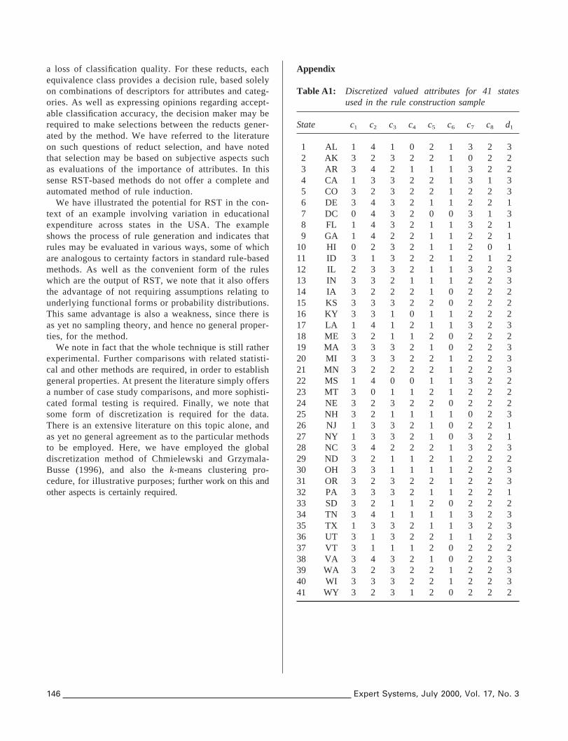
The full list of discretized attribute values (including thedecision attribute value) is given in the Appendix, TableA1. Inspecting this table we note that there are 37 differentcombinations of discretized condition attribute values. Itfollows there are three groups of states, namelyh5, 31, 39j,h18, 33j and h20, 40j, having the same combination ofdiscretized condition attributes (within their groups). Thestates inside each of the individual groups are within thesame cluster, e.g. states 5, 31 and 39 are all within cluster3 (see the Appendix and Figure 2). This factor allows usto give a measure of the consistency of the data, in thiscase unity (see Chmielewski & Grzymala-Busse, 1996).Importantly, since this paper employs the VPRS method,this implies that the quality of approximation needs to beequal to unity for any value ofbmin P (0.5, 1.0].

5. 3. Rough set analysis

The first stage when using VPRS is to calculate theb-reducts for the discretized information in the Appendix,Table A1. Table 7 gives a list of eightb-reducts available.

The table shows us that the number of condition attri-butes in any of the above givenb-reducts ranges from 1(e.g.b-reduct 1) to 7 (e.g.b-reduct 8). Since in this paperwe are following the method of Anet al. (1996), we areconcerned with the minimum value ofb for which theboundary region is empty (thebmin value must also begreater than 0.5) for each associated condition equivalenceclass. Thebmin score for each of theb-reducts is also shownin Table 7. Thebmin values range from 0.538 (b-reduct 1)to 1.00 (b-reduct 8). The fact thatb-reduct 8 hasb = 1implies that each object classified is correctly classified. Ifwe considerb-reduct 5 (i.e.hc1, c3, c8j), then itsbmin valueis 0.571, implying that the minimum conditional probabilityof classifying an object to a manufacturer is 0.571 (i.e. atleast one condition attribute equivalence class has 57.1%of its objects within a single cluster). Hence we considerour level of confidence in predictions made using all theassociated rules.

We have noted previously that the choice ofb-reduct touse depends to a large extent on the decision maker andhave noted suggestions which have been offered in theliterature. In the absence of a particular method of choice,we simply useb-reduct 5 (i.e.hc1, c3, c8j) to illustrate. Mov-ing on to rule construction for this particularb-reduct givesus 12 rules, which classify 41 out of the 41 in-sample states(hence the quality of approximation is unity as required).These rules are given in Table 8.

As we have defined earlier, decision attribute valued1

denotes the clusters of the states shown in Figure 2 takingthe values 1, 2 or 3. Table 8 shows that rules 1–3 classifystates to Cluster 1, rules 4–6 classify to the Cluster 2 andrules 7–12 classify to the final Cluster 3. TheS column

Table 5: Condition attribute intervals for discretization

Attribute Interval ‘0’ Interval ‘1’ Interval ‘2’ Interval ‘3’ Interval ‘4’

c1 [0.0, 40.4) [40.4, 63.6) [63.6, 63.7) [63.7, 100]c2 [0.0, 0.6) [0.6, 0.8) [0.8, 8.2) [8.2, 23.1) [23.1, 100]c3 [0.0, 0.4) [0.4, 1.5) [1.5, 2.7) [2.7, 100]c4 [0.0, 0.7) [0.7, 1.2) [1.2, 100]c5 [0.0, 0.1) [0.1, 0.6) [0.6, 100]c6 [0.0, 15.6) [15.6,̀ )c7 [0.0, 8.4) [8.4, 9.5) [9.5, 19.6) [19.6, 100]c8 [0.0, 8.8) [8.8, 10.3) [10.3, 100]

Table 6: Example of discretization of state conditionattributes

State AL c1 c2 c3 c4 c5 c6 c7 c8

Original 62.1 36.0 0.5 0.6 0.7 16.9 22.6 13.2Discretized 1 4 1 0 2 1 3 2

relates to the strength of each rule, i.e. denotes the numberof states classified by that particular rule. We note that thesum of the values in theS column amounts to 41 (6 withd1 = 1, 11 with d1 = 2 and 24 withd1 = 3), indicating thatall of the 41 in-sample states are assigned a classification.

The P column represents the conditional probability ofeach rule, i.e. the proportion of objects satisfying this ruleand satisfying the decision attribute. We note that rule 1hasP = 0.750 (i.e. three out of four): of the four states withthe same combination of condition attributes (fromhc1, c3,c8j), three states have decision attribute 1 (i.e. FL, NJ andNY) and a single state (i.e. TX) has decision attribute 3.Importantly, rule 7 hasP = 0.571, which is the minimumconditional probability value in the list (hencebmin = 0.571as in Table 7): the value 0.571 follows from the fact that14 states have the same combination of attributes (i.e.c1,c3, c8), of which eight are correctly satisfied. By consideringthe effects of the values in theP column, we see that inthis case a total of 29 out of 41 of the states are cor-rectly classified.

One further important feature shown by thisS column

Table 7: b-reducts of the brand attributes

No. b-reducts bmin No. b-reducts bmin No. b-reducts bmin

1 hc2j 0.538 4 hc1, c5j 0.545 7 hc2, c3, c4, c5, c6, c8j 0.6672 hc4j 0.555 5 hc1, c3, c8j 0.571 8 hc1, c2, c3, c4, c5, c6, c7j 1.0003 hc6j 0.583 6 hc3, c4, c5, c6, c7j 0.667


concerns the number of rules which only classify a singleobject (in this example seven out of the 12 rules). The sep-aration of the rules, between high valued and low valuedstrengths, may be interpreted as signifying differencesbetween states, almost equivalent to labelling certainobjects (states) as ‘outliers’. However, as in many statisticaltechniques where outliers once found are removed from theanalysis, here they are not removed but are allocated totheir specific rules. These rules are potentially importantfor prediction. To illustrate the interpretation of the rules,bringing in the information from the attribute intervalboundaries given in Table 5, we consider rule 4, which wecan fully write out as

(63.7# c1 # 100)` (0.4# c3 , 1.5) JJJ→9 66.7%

(d1 = 2)

or

If the percentage of white students lies between 63.7%and 100%, and the percentage of hispanic students liesbetween 0.4% and 1.5% then the state is in Cluster 2,classifying nine states with 66.7% certainty.

To illustrate the benefit of the use of VPRS we need tolook at the holdout sample group of states, given in theAppendix, Table A2. Using the rules given in Table 8 andthe boundary values for the intervals given in Table 5 wecheck to see if the rules we have constructed for theb-reduct classify the states correctly. First we check to see ifthe condition attributes in theb-reduct exactly match any

Table 8: Decision rules for theb-reduct hc1, c3, c8j

Rule c1 c3 c8 d1 S P

1 If 1 and 3 and 2 Then 1 4 0.7502 If and 0 Then 1 1 13 If 1 and 2 Then 1 1 14 If 3 and 1 Then 2 9 0.6675 If 0 Then 2 1 16 If 3 and 1 Then 2 1 17 If 3 and 3 and 2 Then 3 14 0.5718 If 3 and 2 Then 3 5 0.6009 If 1 and 1 Then 3 2 1

10 If 2 Then 3 1 111 If 1 and 1 Then 3 1 112 If 0 and 1 Then 3 1 1

Table 9: Which rule classifies which state

State

AZ CT MD MO NV NM OK RI SC WV

Rule 11e 7e 1e 4e 7e 1n 7e 7e 9e 5e

rule. For those states which we are unable to match to a ruleexactly, we need to see which rule most closely matches thestate’s relevant condition attributes.

To do this we use a method discussed by Stefanowski(1992) and Slowinski and Stefanowski (1992). The methodcalculates a measure of the distance between each classify-ing rule and each new object. This is computed only forattributes present in each rule. We take each given newobject x to be described by valuesc1(x), c2(x), . . ., cm(x)for the condition attributes, withm # card(C). Similarly,we havec1(y), c2(y), . . ., cm(y) of the samem conditionattributes for available rules. It follows that the distance ofobjectx from rule y is measured by

D =1m SOm

l = 1

HklF|cl(x) − cl(y)|vl

max − vlmin GpJD1/p

wherep = 1, 2, . . . is a natural number to be chosen by ananalyst, vl

max, vl

minare the maximal and minimal values

respectively ofcl, kl is the importance coefficient of cri-terion cl and m is the number of condition attributes in arule. For this case we have usedp = 2 andkl = 1 for all l.The value ofp chosen determines the importance of thenearest rule. A small value ofp allows a major difference


on one criterion to be compensated by a number of minordifferences on other criteria, whereas high values ofp willover-value the larger differences and ignore minor differ-ences. We employ a value ofp = 2, thereby implicitly con-sidering ‘least squares’ fitting for each rule. When consider-ing the method of finding the nearest rule, we acknowledgean alternative method discussed by Slowinski (1993) whichis based on a ‘valued closeness relation’. The method putsmore emphasis on subjective assessments of the importancevalues of the attributes by professional experts and is there-fore less suitable for statistical work.

After applying the rules in Table 8 (using the definedintervals in Table 5) to the data in the Appendix, Table A2,we find 70.0% (seven out of 10) of the states are correctlyclassified. We can illustrate this by looking at the rulesmatching with each state from the holdout sample group.

Table 9 provides an illustration. For each state we givethe relevant rule, with an ‘e’ superscript indicating exactrule classification and an ‘n’ indicating a nearest rule classi-fication. If a rule, whether exact or nearest, classifies anobject wrongly then the rule number is shown in boldfaceand underlined (i.e. states CT, NM and OK). We can finallygive an indication of the strength of each rule (see Table10) in terms of its use in the prediction of the holdout sam-ple states.

Where a number in brackets appears in these columns,it denotes a rule chosen which wrongly classified that num-ber of states. An interesting case is rule 11, which one couldthink of as a rule classifying an outlier in the original ruleconstruction. For rule 11,S = 1 in Table 8; in the holdoutsample states the rule correctly classifies the state AZ, illus-trating the advantage of keeping what might be seen to beoutlier objects within the system. With the holdout samplestates each classified by a rule, Figure 3 shows a scatter

Table 10: Strength of rules with respect to the holdoutsample states

Rule 1 2 3 4 5 6 7 8 9 10 11 12

Strength 1 (1) 0 0 1 1 0 2 (2) 0 1 0 1 0

Figure 3: Scatter plot visualization of rules.

plot diagram similar to that in Figure 2 but with states rep-resented by the rule which classifies them.

Within Figure 3, those states in the holdout sample groupand hence predicted are signified with a ‘p’ superscript,and those states mis-classified (in-sample or holdoutsample) by a rule are underlined. We noted earlier thatrule 11 (with S = 1) correctly classified a state in theholdout sample; Figure 3 shows that the two states classi-fied (in-sample and holdout sample) by rule 11 are nextto each other and away from other states. Indeed thesestates AZ and CA (from the USA map in Figure 2) areneighbouring states (geographically).

6. A comparison with discriminant analysis

Given that the primary purpose of VPRS is to generaterules for classification, the most closely related ‘classical’


statistical technique is discriminant analysis. In this sectionwe present the results of a standard linear discriminantanalysis (LDA) and provide some comparisons with theVPRS model described above. Standard LDA involves alinear classification boundary, but it should be noted thatit depends on assumptions regarding normality of theunderlying populations, which must also possess identicalvariance–covariance matrices. The linear rule can be shownto minimize the expected number of misclassifications (seefor example Johnson & Wichern, 1998). VPRS does notoperate with a specific functional form, nor does it requiredistributional assumptions. Table 11 gives a comparisonbetween the results of LDA (used on the original continu-ous values of the condition attributes) and VPRS.

7. Summary and conclusions

RST, which for our purposes includes its probabilisticgeneralization VPRS, is a novel method for rule induc-tion and classification. It began as a general method forapproximating a set, but is most applicable in a super-vised learning context. The method is based on a novelclassification metric, implemented as upper and lowerapproximations of a set and more generally in terms ofpositive, negative and boundary regions. Classificationaccuracy, which may be set by the decision maker, ismeasured in terms of conditional probabilities for equiv-alence classes, and the method involves a search for sub-sets of attributes (called ‘reducts’) which do not require

Table 11: Comparison of results between LDA and VPRS

Sample Predicted Percentage Totalclassifications correct correct

‘1’ ‘2’ ‘3’

LDA usinghc1, c2, c3, c4, c5, c6, c7, c8jIn sample ‘1’ 4 0 3 57.14% 82.93%

‘2’ 0 13 1 92.86%‘3’ 3 0 17 85.00%

Out of ‘1’ 2 0 0 100.00% 60.00%sample ‘2’ 0 3 1 75.00%

‘3’ 1 2 1 25.00%

VPRS analysis onb-reduct hc1, c3, c8jIn sample ‘1’ 5 0 2 71.43% 70.73%

‘2’ 0 8 6 57.14%‘3’ 1 3 16 80.00%

Out of ‘1’ 1 0 1 50.00% 70.00%sample ‘2’ 1 2 1 50.00%

‘3’ 0 0 4 100.00%

a loss of classification quality. For these reducts, eachequivalence class provides a decision rule, based solelyon combinations of descriptors for attributes and categ-ories. As well as expressing opinions regarding accept-able classification accuracy, the decision maker may berequired to make selections between the reducts gener-ated by the method. We have referred to the literatureon such questions of reduct selection, and have notedthat selection may be based on subjective aspects suchas evaluations of the importance of attributes. In thissense RST-based methods do not offer a complete andautomated method of rule induction.

We have illustrated the potential for RST in the con-text of an example involving variation in educationalexpenditure across states in the USA. The exampleshows the process of rule generation and indicates thatrules may be evaluated in various ways, some of whichare analogous to certainty factors in standard rule-basedmethods. As well as the convenient form of the ruleswhich are the output of RST, we note that it also offersthe advantage of not requiring assumptions relating tounderlying functional forms or probability distributions.This same advantage is also a weakness, since there isas yet no sampling theory, and hence no general proper-ties, for the method.

We note in fact that the whole technique is still ratherexperimental. Further comparisons with related statisti-cal and other methods are required, in order to establishgeneral properties. At present the literature simply offersa number of case study comparisons, and more sophisti-cated formal testing is required. Finally, we note thatsome form of discretization is required for the data.There is an extensive literature on this topic alone, andas yet no general agreement as to the particular methodsto be employed. Here, we have employed the globaldiscretization method of Chmielewski and Grzymala-Busse (1996), and also thek-means clustering pro-cedure, for illustrative purposes;further work on this andother aspects is certainly required.


Appendix

Table A1: Discretized valued attributes for 41 statesused in the rule construction sample

State c1 c2 c3 c4 c5 c6 c7 c8 d1

1 AL 1 4 1 0 2 1 3 2 32 AK 3 2 3 2 2 1 0 2 23 AR 3 4 2 1 1 1 3 2 24 CA 1 3 3 2 2 1 3 1 35 CO 3 2 3 2 2 1 2 2 36 DE 3 4 3 2 1 1 2 2 17 DC 0 4 3 2 0 0 3 1 38 FL 1 4 3 2 1 1 3 2 19 GA 1 4 2 2 1 1 2 2 1

10 HI 0 2 3 2 1 1 2 0 111 ID 3 1 3 2 2 1 2 1 212 IL 2 3 3 2 1 1 3 2 313 IN 3 3 2 1 1 1 2 2 314 IA 3 2 2 2 1 0 2 2 215 KS 3 3 3 2 2 0 2 2 216 KY 3 3 1 0 1 1 2 2 217 LA 1 4 1 2 1 1 3 2 318 ME 3 2 1 1 2 0 2 2 219 MA 3 3 3 2 1 0 2 2 320 MI 3 3 3 2 2 1 2 2 321 MN 3 2 2 2 2 1 2 2 322 MS 1 4 0 0 1 1 3 2 223 MT 3 0 1 1 2 1 2 2 224 NE 3 2 3 2 2 0 2 2 225 NH 3 2 1 1 1 1 0 2 326 NJ 1 3 3 2 1 0 2 2 127 NY 1 3 3 2 1 0 3 2 128 NC 3 4 2 2 2 1 3 2 329 ND 3 2 1 1 2 1 2 2 230 OH 3 3 1 1 1 1 2 2 331 OR 3 2 3 2 2 1 2 2 332 PA 3 3 3 2 1 1 2 2 133 SD 3 2 1 1 2 0 2 2 234 TN 3 4 1 1 1 1 3 2 335 TX 1 3 3 2 1 1 3 2 336 UT 3 1 3 2 2 1 1 2 337 VT 3 1 1 1 2 0 2 2 238 VA 3 4 3 2 1 0 2 2 339 WA 3 2 3 2 2 1 2 2 340 WI 3 3 3 2 2 1 2 2 341 WY 3 2 3 1 2 0 2 2 2

Table A2: Continuous valued attributes for 10 statesused in the holdout sample

State c1 c2 c3 c4 c5 c6 c7 c8 d1

1 AZ 56.9 4.3 30.0 1.7 7.2 19.6 24.2 10.2 32 CT 72.0 13.5 11.8 2.4 0.3 14.4 17.8 14.7 13 MD 57.5 35.0 3.3 3.8 0.3 16.8 13.3 12.5 14 MO 81.7 16.1 1.0 1.0 0.2 15.4 9.8 13.6 25 NV 66.5 9.8 17.2 4.5 1.9 19.1 11.1 10.6 36 NM 39.5 2.4 46.8 1.0 10.4 17.0 34.9 14.4 27 OK 69.4 10.5 3.9 1.3 15.0 15.7 24.2 11.6 28 RI 78.9 7.0 10.3 3.3 0.5 14.3 16.4 16.7 39 SC 56.3 42.1 0.7 0.8 0.2 16.2 31.7 13.4 3

10 WV 95.2 4.0 0.3 0.4 0.1 14.6 25.8 15.1 2

References

An, A., N. Shan, C. Chan, N. Cercone andW. Ziarko (1996)Discovering rules for water demand prediction: an enhancedrough-set approach,Engineering Applications of ArtificialIntellgence, 9 (6), 645–653.

Bjorvand, A.T. (1996)Time series and rough sets, Master’s The-sis, Knowledge Systems Group, Department of Computer Sys-tems and Telematics, Faculty of Electrical Engineering andComputer Science, The Norwegian Institute of Technology,University of Trondheim.

Browne, C., I. Duntsch andG. Gediga (1998) IRIS revisited:a comparison of discriminant and enhanced rough set dataanalysis, in Rough Sets in Knowledge Discovery 2: Appli-cations, Case Studies and Software Systems, L. Polkowski andA. Skowron (eds.), Heidelberg: Physica, 345–368.

Chmielewski, M.R. and J.W. Grzymala-Busse (1996) Globaldiscretization of continuous attributes as preprocessing formachine learning, International Journal of ApproximateReasoning, 15, 319–331.

Dimitras, A., R. Slowinski, R. Susmaga and C. Zopounidis(1999) Business failure using rough sets,European Journal ofOperational Research, 114, 263–280.

Everitt, B. (1993) Cluster Analysis, 3rd edn, London: Heine-mann Educational.

Fayyad, U.M. andK.B. Irani (1992) On the handling of continu-ous-valued attributes in decision tree generation,MachineLearning, 8, 87–102.

Getis, A. (1999) Some thoughts on the impact of large data setson regional science,Annals of Regional Science, 33, 145–150.

Jelonek, J., K. Krawiec and R. Slowinski (1995) Rough setreduction of attributes and their domains for neural networks,Computational Intelligence, 11 (2), 339–347.

Johnson, R.A. andD.W. Wichern (1998)Applied MultivariateStatistical Analysis, 4th edn, Upper Saddle River, NJ:Prentice Hall.

Krawiec, K., R. Slowinski and D. Vanderpooten (1998)Learning decision rules from similarity based rough approxi-mations, in Rough Sets in Knowledge Discovery 2: Appli-cations, Case Studies and Software Systems, L. Polkowski andA. Skowron (eds), Heidelberg: Physica, 37–54.

Krusinska, E., R. Slowinski andJ. Stefanowski (1992) Discri-minant versus rough set approach to vague data analysis,Applied Stochastic Models and Data Analysis, 8, 43–56.

Moraczewski, I.R., B. Sudnik-Wojcikowska andW. Borkow-


ski (1996) Rough sets in floristic description of the inner-cityof Warsaw,FLORA, 191, 253–260.

Pawlak, Z. (1982) Rough sets,International Journal of Infor-mation and Computer Sciences, 11 (5), 341–356.

Pawlak, Z. (1991)Rough Sets — Theoretical Aspects of Reason-ing about Data, London: Kluwer Academic.

Pawlak, Z. (1998) Foreword, inRough Sets in Knowledge Dis-covery 2: Applications, Case Studies and Software Systems, L.Polkowski and A. Skowron (eds), Heidelberg: Physica, V.

Pawlak, Z., J. Grzymala-Busse, R. Slowinski andW. Ziarko(1995) Rough sets,Communications of the ACM, 38 (11),89–95.

Skowron, A. andJ.W. Grzymala-Busse (1994) From the roughset theory to evidence theory, inAdvances in the Dempster–Shafer Theory of Evidence, R.Y. Ronald, M. Fedrizzi and J.Kacprzyk (eds), New York: Wiley, 193–236.

Slowinski, R. (1993) Rough set learning of preferential attitudein multi-criteria decision making, inMethodologies for Intelli-gent Systems, Lecture Notes in Artificial Intelligence 689, J.Komorowski and Z.W. Ras (eds), Berlin: Springer, 642–651.

Slowinski, R. and J. Stefanowski (1992) RoughDAS andRoughClass software implementations of the rough setsapproach, inIntelligent Decision Support. Applications andAdvances of the Rough Sets Theory, R. Slowinski (ed.), Lon-don: Kluwer Academic.

Slowinski, R., C. Zopounidis andA.I. Dimitras (1997) Predic-tion of company acquisition in Greece by means of the roughset approach,European Journal of Operational Research, 100,1–15.

Stefanowski, J. (1992) Classification support based on the roughset theory,Proceedings, IIASA Workshop on User-orientedMethodology and Techniques of Decision Analysis and Sup-port, Serock, 1991. Heidelberg: Springer.

Szczuka, M.S. (1998) Rough sets and artificial neural networks,Rough Sets in Knowledge Discovery 2: Applications, CaseStudies and Software Systems, L. Polkowski and A. Skowron(eds), Heidelberg: Physica, 449–470.

Wakulicz-Deja, A. andP. Paszek (1997) Diagnose progressiveencephalopathy applying the rough set approach,InternationalJournal of Medical Informatics, 46, 119–127.

Ziarko, W. (1993a) Rough sets and knowledge discovery: anoverview,Proceedings of the International Workshop on RoughSets and Knowledge Discovery (RSKD’93), Banff, Alberta,Canada.

Ziarko, W. (1993b) Variable precision rough set model,Journalof Computer and System Sciences, 46, 39–59.

Ziarko, W. (1993c) Analysis of uncertain information in theframework of variable precision rough sets,Foundations ofComputing Decision Sciences, 18, 381–396.

The authors

Malcolm Beynon

Malcolm Beynon received his BSc and PhD in mathematicsfrom the University of Wales, Cardiff. In 1993 be becamea Lecturer in the Computing Mathematics Department ofCardiff University and in 1995 he took up his currentposition of Lecturer at Cardiff Business School. Hisresearch interests range from his PhD work investigatingKolmogorov-type integral inequalities to the analytical

theory of neural networks. He is also working on moderndata analysis techniques including Dempster–Shafer theoryand rough set theory.

Bruce Curry

Bruce Curry is Senior Lecturer in Computing at CardiffBusiness School, Cardiff University. His background is ineconometrics and operations research, but he also hasinterests in information technology. In recent years he hasdone research on expert systems in marketing. His currentinterests centre mainly on neural network techniques andapplications, but also include wider aspects of decision sup-port modelling.


Peter Morgan

Peter Morgan originally graduated in industrial chemistryfrom the University of Wales and then gained a PhD inpolymer physical chemistry. His subsequent careerincluded fundamental research in chemical microwavespectroscopy and spectroscopic data analysis, as well asindustrial liaison in technology transfer and innovationtraining. He is currently a Lecturer in Quantitative Analysisat Cardiff Business School with research interests in optim-ization applied to business problems and data analysis withneural networks.

Classification and rule induction using rough set theory

Documents

Transcript of Classification and rule induction using rough set theory