1

Rule Induction for Automatic Configuration of Planning Systems

Dimitris Vrakas DVRAKAS@CSD.AUTH.GR Grigorios Tsoumakas GREG@CSD.AUTH.GR Nick Bassiliades NBASSILI@CSD.AUTH.GR Ioannis Vlahavas VLAHAVAS @CSD.AUTH.GR Department of Informatics, Aristotle University of Thessaloniki, Thessaloniki 54124, GREECE

Abstract This paper presents a methodology for building an adaptive planning system, which automatically fine-tunes its planning parameters according to the morphology of the problem in hand, through a combination of Planning, Machine Learning and Knowledge-Based techniques. The adaptation is guided by a rule-based system that sets planner configuration parameters based on measurable characteristics of the problem instance. The knowledge of the rule system has been acquired through a rule induction algorithm. Specifically, the approach of propositional rule learning was applied to a dataset produced by results from experiments on a large number of problems from various domains, including those used in the three International Planning Competitions. The validity of our methodology is assessed through thorough experimental results that demonstrate the boost in performance of the planning system in problems of both known and unknown domains.

1. Introduction

In domain independent heuristic planning there is a number of systems that their performance varies between best and worse on a number of toy and real-world planning domains. No planner has been proved yet to be the best for all kinds of problems and domains. Similar instability in their efficiency is also noted when different variations of the same planner are tested on the same problem, when the value of one or more parameters of the planner is changed. Although most planners claim that the default values for their options guarantee a stable and averagely good performance, in most cases fine tuning the parameters by hand improves the performance of the system for the given problem. Few attempts have been made to explain which are the specific dynamics of a planning problem that favor a specific planning system and even more, which is the best setup for a planning system given the characteristics of the planning problem. This kind of knowledge would clearly assist the planning community in producing flexible systems that could automatically adapt themselves to each problem, achieving best performance. In this paper, we used a large dataset with results from executions of our planning system, called HAP (Highly Adjustable Planner), on various problems and we employed machine learning techniques to discover knowledge that associates measurable characteristics of the planning problems with specific values for the parameters of the planning system. The selection of these characteristics was very carefully made, emphasizing on balancing the mixture of characteristics that are independent, semi-dependent and dependent on the specific planning system used for the research. The knowledge, acquired by the process of machine learning, was embedded in the planner in the form of a rule-based system, which can automatically change its configuration to best suit the current problem. The performance of the resulting planning system was thoroughly evaluated through experiments that aimed at showing the behavior of the adaptive system in a) unknown problems of known domains, b) unseen domains, c) harder problems of known domains, d) a

2

single domain and e) comparison with three state-of-the-art domain independent planning systems. The results showed that the system managed to adapt quite well in all the experiments and to be competitive compared to the other planning systems. The rest of the paper is organized as follows: Section 2 presents a survey of related work combining Machine Learning and Planning. The next section outlines the complete methodology we followed in this work. The planning system used for the purposes of our research and the problem analysis done for deciding the problem attributes are presented in sections 4 and 5, respectively. Section 6 describes in detail the learning methodology we followed and Section 7 discusses how the learned model was embedded as a rule system in the adaptive planner. Section 8 presents and discusses the experimental results and finally, Section 9 concludes the paper and poses future research directions.

2. Related Work

Machine learning has been extensively exploited in the past to support Planning systems in many ways. Since it is a usual case for seemingly different planning problems to present similarities in their structure, it is reasonable enough to believe that planning strategies that have been successfully applied to some problems in the past will be also effective for similar problems in the future. Learning can assist planning systems in three ways: a) to learn domain knowledge, b) to learn control knowledge and c) to learn optimization knowledge. Domain knowledge is utilized by planners in pre-processing phases in order to either modify the description of the problem in a way that it will make it easier for solving or make the appropriate adjustments to the planner to best attack the problem. Control knowledge can be utilized during search in order to either solve the problem faster or produce better plans. For example, the knowledge extracted from past examples can be used to refine the heuristic functions or create a guide for pruning non-promising branches. Finally, optimization knowledge is utilized after the production of an initial plan, in order to transform it in a new one that optimizes certain criteria, e.g. number of steps or resources usage. Most approaches in the past have focused on ways for learning control knowledge since it is crucial for planners to have an informative guide during search. The PRODIGY Architecture (Carbonell, Knoblock and Minton 1991, Veloso et al. 1995) was the main representative of this trend. This architecture, supported by various learning modules, focuses on learning the necessary knowledge (rules) that guides a planner to decide what action to take next during plan execution. Since the overhead of testing the applicability of rules was quite large (utility problem) the system also adopted a mixed criterion of usability and cost for each rule in order to discard some of them. Although PRODIGY is the most known system integrating planning and learning, the history of learning control knowledge for guiding planning systems dates back to the early 70’s. The STRIPS planning system was quickly enhanced with a learning module (Fikes, Hart and Nilsson 1972) that analyzed past experience from solved problems in order to infer macro-operators, which represented successful combinations of action sequences, and general conditions for applying these macro-operators. DYNA-Q (Sutton 1990) uses Q-learning, a form of reinforcement learning, in order to accompany each pair of state-action with a reward (Q-value). The rewards maintained by DYNA-Q are incrementally updated as new problems are faced and are utilized during search as a means of heuristic function. The main problems faced by this approach were the very large memory requirements and the amount of experience needed for solving non-trivial problems.

3

Borrajo and Veloso (1996) also developed HAMLET, another system combining planning and learning that was built on top of PRODIGY. HAMLET combines deductive and inductive learning strategies in order to incrementally learn through experience. The main aspect responsible for the efficiency of the system are: the lazy explanation of successes, the incremental refinement of acquired knowledge and the lazy learning to override only the default behavior of the planner. Another learning approach that has been applied on PRODIGY, is the STATIC algorithm (Etzioni 1993), which uses Partial Evaluation (PE) instead of EBL to automatically extract search-control knowledge from training examples. A more recent approach of learning control knowledge for domain independent planning was presented by Martin and Geffner (2000). In their research they focus on learning generalized policies that serve as heuristic functions, mapping states and goals into actions. In order to represent their policies they adopt a concept language, which allows the inference of more accurate models using less training examples. Another example of utilizing learning techniques for inferring control knowledge for automated planning systems is the family of case-based planners, such as CHEF (Hammond 1989) or PRIAR (Kambhampati and Hendler 1992). CHEF is one of the earliest case-based planners and used the Szechwan cooking as the application domain. CHEF used memory structures and indexes in order to store successful plans, failed plans and repairs among with general conditions allowing it to reuse past experience. PRIAR is a more general case-based system for plan modification and reuse that uses hierarchical non-linear planning, allowing abstraction and least-commitment. Apart from learning control knowledge there has been a number of works focusing on learning domain knowledge. For example, Wang’s OBSERVER (Wang 1996) is a learning system, build on top of the PRODIGY system, that uses expert’s hints and past knowledge in order to extract and refine the full description of the operators for a new domain. The description of the operators include preconditions and effects (negative and positive), allowing also conditional effects and preconditions. Knoblock (1990) presented another learning module for the PRODIGY system, called ALPINE, that learns abstraction hierarchies and thus reducing the required search. MULTI-TAC (Minton, 1996) is a learning system which uses a library of heuristics and generic algorithms and automatically fine tunes itself in order to synthesize the most appropriate constraint satisfaction program to solve a problem. The methodology we followed in this paper presents some similarities with MULTI-TAC. Probably, the only approach to the direction of adaptive planning done in the past is the work presented in (Howe and Dahlman, 1993, Howe et al, 1999). They have created a system called BUS, which incorporates six state-of-the-art planners (STAN, IPP, SGP, BlackBox, UCPOP and Prodigy) and runs them using a round-robin schema, until one of them finds a solution. BUS is adaptable in the sense of deciding the ordering of the six planners and the duration of the time slices dynamically based on the values of five problem characteristics and some rules extracted from a statistical analysis on past runs. The system achieved more stable behavior but it was not as fast as one may have expected. This paper extends and completes previous research by the authors on learning domain knowledge for adaptive planning (Vrakas et al., 2003). In that work the method of classification based on association rules was followed to learn rules for configuring a previous version of HAP. That work used a limited number of problem attributes that were not adequate enough to capture the dynamics of certain problems and the learning methodology required discrete values which had an impact on the accuracy of the model. Furthermore, the experimental results covered only a few aspects of the methodology potentials.

4

The third option of learning for Planning (optimization learning) concerns the extraction of knowledge that will assist in the modification of the extracted plans. Ambite, Knoblock and Minton (2000) have presented an approach for the automatic learning of Plan Rewriting Rules, that can be utilized along with some local search, in order to improve easy-to-generate low quality plans. Zimmerman and Kambhampati (2003) have presented a very detailed and analytical survey of past approaches combining Planning and Machine Learning. Additional information about learning-powered adaptive planners can be found in (Gopal 2000).

3. Methodology Outline

We will here briefly sketch the methodology for learning a rule base, embedding it in our adaptive planner and evaluating its performance. All the steps that are outlined here will be described in more detail in the following sections.

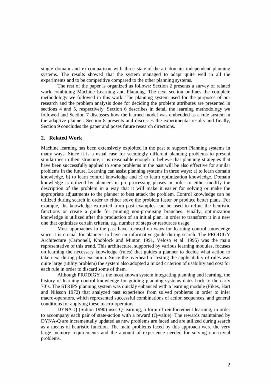
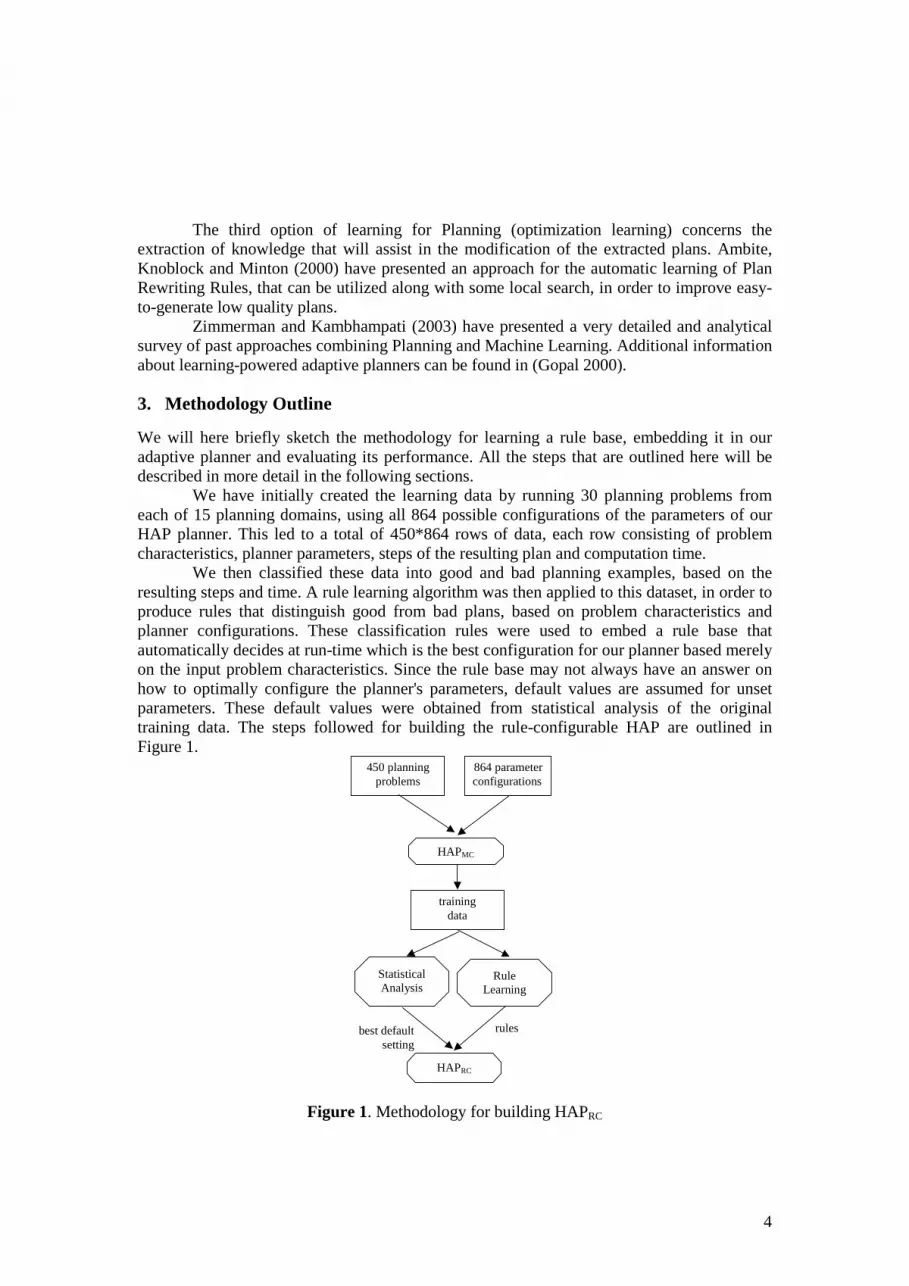
We have initially created the learning data by running 30 planning problems from each of 15 planning domains, using all 864 possible configurations of the parameters of our HAP planner. This led to a total of 450*864 rows of data, each row consisting of problem characteristics, planner parameters, steps of the resulting plan and computation time.

We then classified these data into good and bad planning examples, based on the resulting steps and time. A rule learning algorithm was then applied to this dataset, in order to produce rules that distinguish good from bad plans, based on problem characteristics and planner configurations. These classification rules were used to embed a rule base that automatically decides at run-time which is the best configuration for our planner based merely on the input problem characteristics. Since the rule base may not always have an answer on how to optimally configure the planner's parameters, default values are assumed for unset parameters. These default values were obtained from statistical analysis of the original training data. The steps followed for building the rule-configurable HAP are outlined in Figure 1.

450 planning problems

864 parameter configurations

training data

Rule Learning

Statistical Analysis

HAPRC

best default setting

rules

HAPMC

Figure 1. Methodology for building HAPRC

5

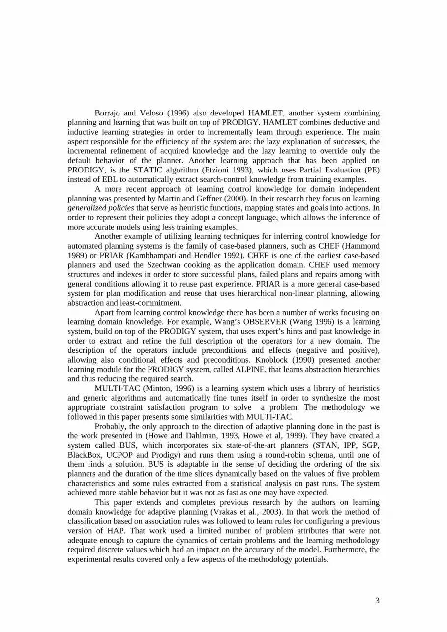
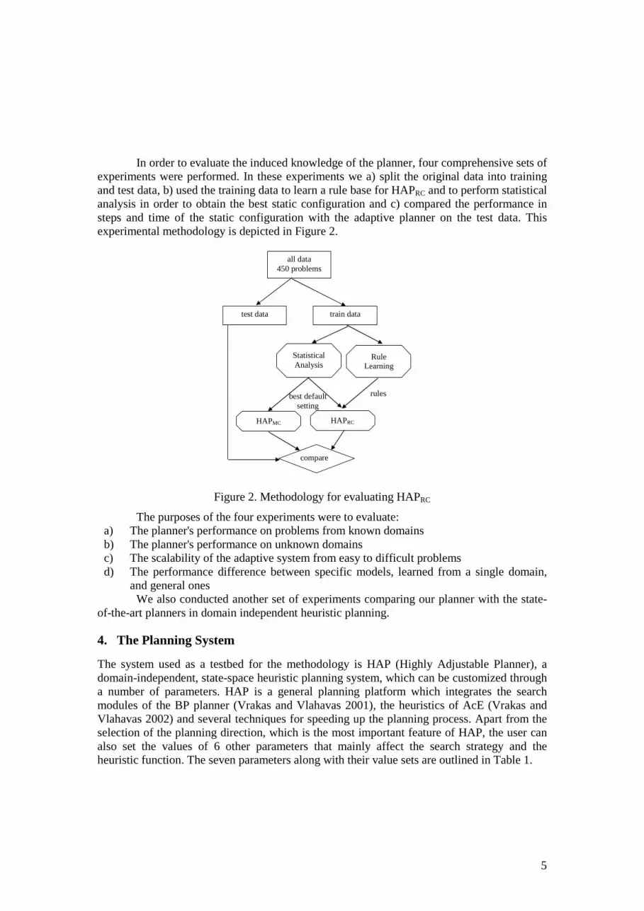
In order to evaluate the induced knowledge of the planner, four comprehensive sets of experiments were performed. In these experiments we a) split the original data into training and test data, b) used the training data to learn a rule base for HAPRC and to perform statistical analysis in order to obtain the best static configuration and c) compared the performance in steps and time of the static configuration with the adaptive planner on the test data. This experimental methodology is depicted in Figure 2.

test data train data

all data 450 problems

Rule Learning

Statistical Analysis

HAPRC

best default setting

rules

HAPMC

compare

Figure 2. Methodology for evaluating HAPRC

The purposes of the four experiments were to evaluate: a) The planner's performance on problems from known domains b) The planner's performance on unknown domains c) The scalability of the adaptive system from easy to difficult problems d) The performance difference between specific models, learned from a single domain,

and general ones We also conducted another set of experiments comparing our planner with the state-

of-the-art planners in domain independent heuristic planning.

4. The Planning System

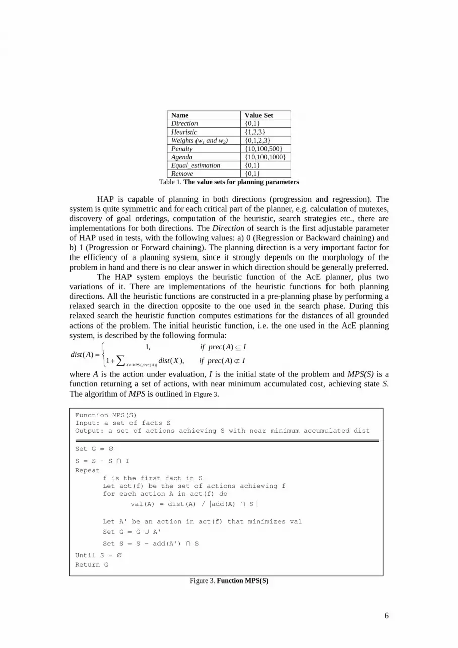
The system used as a testbed for the methodology is HAP (Highly Adjustable Planner), a domain-independent, state-space heuristic planning system, which can be customized through a number of parameters. HAP is a general planning platform which integrates the search modules of the BP planner (Vrakas and Vlahavas 2001), the heuristics of AcE (Vrakas and Vlahavas 2002) and several techniques for speeding up the planning process. Apart from the selection of the planning direction, which is the most important feature of HAP, the user can also set the values of 6 other parameters that mainly affect the search strategy and the heuristic function. The seven parameters along with their value sets are outlined in Table 1.

6

Name Value Set Direction {0,1} Heuristic {1,2,3} Weights (w1 and w2) {0,1,2,3} Penalty {10,100,500} Agenda {10,100,1000} Equal_estimation {0,1} Remove {0,1}

Table 1. The value sets for planning parameters

HAP is capable of planning in both directions (progression and regression). The system is quite symmetric and for each critical part of the planner, e.g. calculation of mutexes, discovery of goal orderings, computation of the heuristic, search strategies etc., there are implementations for both directions. The Direction of search is the first adjustable parameter of HAP used in tests, with the following values: a) 0 (Regression or Backward chaining) and b) 1 (Progression or Forward chaining). The planning direction is a very important factor for the efficiency of a planning system, since it strongly depends on the morphology of the problem in hand and there is no clear answer in which direction should be generally preferred. The HAP system employs the heuristic function of the AcE planner, plus two variations of it. There are implementations of the heuristic functions for both planning directions. All the heuristic functions are constructed in a pre-planning phase by performing a relaxed search in the direction opposite to the one used in the search phase. During this relaxed search the heuristic function computes estimations for the distances of all grounded actions of the problem. The initial heuristic function, i.e. the one used in the AcE planning system, is described by the following formula:

( ( ))

1, ( )( )

1 ( ), ( )X MPS prec A

if prec A Idist A

dist X if prec A I�

� � ��

� � � �

��

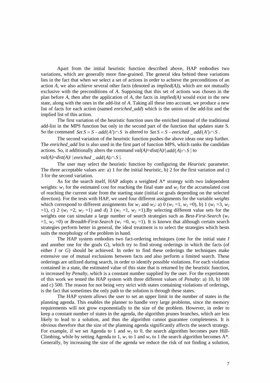
where A is the action under evaluation, I is the initial state of the problem and MPS(S) is a function returning a set of actions, with near minimum accumulated cost, achieving state S. The algorithm of MPS is outlined in Figure 3. Function MPS(S)

Input: a set of facts S Output: a set of actions achieving S with near minimum accumulated dist

Set G = �

S = S – S � I

Repeat f is the first fact in S Let act ( f ) be the set of actions achieving f for each action A in act ( f ) do

val ( A) = dist ( A) / �add ( A) � S��

Let A' be an action in act ( f ) that minimizes val

Set G = G � A'

Set S = S – add ( A' ) � S

Until S = �

Return G

Figure 3. Function MPS(S)

7

Apart from the initial heuristic function described above, HAP embodies two variations, which are generally more fine-grained. The general idea behind these variations lies in the fact that when we select a set of actions in order to achieve the preconditions of an action A, we also achieve several other facts (denoted as implied(A)), which are not mutually exclusive with the preconditions of A. Supposing that this set of actions was chosen in the plan before A, then after the application of A, the facts in implied(A) would exist in the new state, along with the ones in the add-list of A. Taking all these into account, we produce a new list of facts for each action (named enriched_add) which is the union of the add-list and the implied list of this action. The first variation of the heuristic function uses the enriched instead of the traditional add-list in the MPS function but only in the second part of the function that updates state S. So the command ( ')Set S S add A S� � � is altered to _ ( ')Set S S enriched add A S� � � . The second variation of the heuristic function pushes the above ideas one step further. The enriched_add list is also used in the first part of function MPS, which ranks the candidate actions. So, it additionally alters the command val(A)=dist(A)/| ( )add A S� | to val(A)=dist(A)/ | _ ( )enriched add A S� |. The user may select the heuristic function by configuring the Heuristic parameter. The three acceptable values are: a) 1 for the initial heuristic, b) 2 for the first variation and c) 3 for the second variation. As for the search itself, HAP adopts a weighted A* strategy with two independent weights: w1 for the estimated cost for reaching the final state and w2 for the accumulated cost of reaching the current state from the starting state (initial or goals depending on the selected direction). For the tests with HAP, we used four different assignments for the variable weights which correspond to different assignments for w1 and w2: a) 0 (w1 =1, w2 =0), b) 1 (w1 =3, w2 =1), c) 2 (w1 =2, w2 =1) and d) 3 (w1 =1, w2 =1).By selecting different value sets for the weights one can simulate a large number of search strategies such as Best-First-Search (w1 =1, w2 =0) or Breadth-First-Search (w1 =0, w2 =1). It is known that although certain search strategies perform better in general, the ideal treatment is to select the strategies which bests suits the morphology of the problem in hand. The HAP system embodies two fact-ordering techniques (one for the initial state I and another one for the goals G), which try to find strong orderings in which the facts (of either I or G) should be achieved. In order to find these orderings the techniques make extensive use of mutual exclusions between facts and also perform a limited search. These orderings are utilized during search, in order to identify possible violations. For each violation contained in a state, the estimated value of this state that is returned by the heuristic function, is increased by Penalty, which is a constant number supplied by the user. For the experiments of this work we tested the HAP system with three different values of Penalty: a) 10, b) 100 and c) 500. The reason for not being very strict with states containing violations of orderings, is the fact that sometimes the only path to the solution is through these states.

The HAP system allows the user to set an upper limit in the number of states in the planning agenda. This enables the planner to handle very large problems, since the memory requirements will not grow exponentially to the size of the problem. However, in order to keep a constant number of states in the agenda, the algorithm prunes branches, which are less likely to lead to a solution, and thus the algorithm cannot guarantee completeness. It is obvious therefore that the size of the planning agenda significantly affects the search strategy. For example, if we set Agenda to 1 and w2 to 0, the search algorithm becomes pure Hill-Climbing, while by setting Agenda to 1, w1 to 1 and w2 to 1 the search algorithm becomes A*. Generally, by increasing the size of the agenda we reduce the risk of not finding a solution,

8

even if at least one exists, while by reducing the size of the agenda the search algorithm becomes faster and we ensure that the planner will not run out of memory. For the tests we used three different settings for the size of the agenda: a) 10, b) 100 and c) 1000.

Another parameter of HAP is Equal_estimation that defines the way in which states with the same estimated distances are treated. If Equal_estimation is set to 0 then between two states with the same value in the heuristic function, the one with the largest distance from the starting state (number of actions applied so far) is preferred. If Equal_estimation is set to 1, then the search strategy will prefer the state that is closer to the starting state.

HAP also embodies a technique for simplifying the definition of the sub-problem in hand. This technique eliminates from the definition of the sub-problem (current state and goals) all the goals that have already been achieved in the current state and do not interfere with the achievement of the remaining goals. In order to do this, the technique performs off-line before the search process, a dependency analysis on the goals of the problem. Although the technique is very useful in general, the dependency analysis is not complete. In other words, there are cases where an already achieved sub-goal should be temporarily destroyed in order to continue with the achievement of the rest of the goals. Therefore, by removing this fact from the current state the algorithm may risk completeness. The parameter Remove is used to turn on (value 1) and off (value 0) this feature of the planning system.

5. Problem Attributes

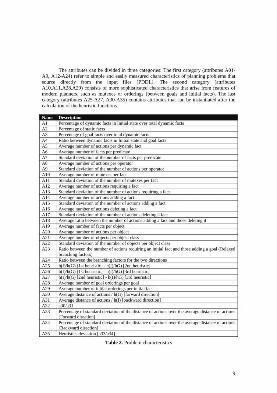
The purpose of this research effort was to discover interesting knowledge that associates the characteristics of a planning problem with the parameters of HAP and leads to good performance. Therefore, a first necessary step that we performed was a theoretical analysis of a planning problem, in order to discover salient characteristics that could potentially influence the choice of parameters of HAP. This resulted in a set of 35 measurable characteristics that are presented in Table 2. In the attributes presented in Table 2, h(I) refers to the number of steps needed to reach I (initial state) by regressing the goals, as this distance is estimated by the backward heuristic. Similarly, h(G) refers to the number of steps needed to reach the goals by progressing the initial state, as this is estimated by the forward heuristic.

Our main concern was to select attributes that their values are easily calculated and not complex attributes that would cause a large overhead in the total planning time. Therefore, most of the attributes come from the PDDL files, which are input to the planner, and their values can be calculated during the standard parsing process. We also included a small number of attributes which are closely related to specific features of the HAP planning system such as the heuristics or the fact-ordering techniques. In order to calculate the values of these attributes, the system must perform a limited search but the overhead is negligible compared to the total planning time.

A second concern which influenced the selection of attributes was the fact that the attributes should be general enough to be applied to all domains and their values should not depend so much on the size of the problem. Otherwise the knowledge learned from easy problems would not be applied effectively to difficult ones. For example, instead of using the number of mutexes (mutual exclusions between facts) in the problem as an attribute that strongly depends on the size of the problem (larger problems tend to have more mutexes), we divide it by the total number of dynamic facts (attribute A10) and this attribute (mutex density) identifies the complexity of the problem without taking into account whether it is a large problem or a not. This is a general solution followed in all situations where a problem attribute depends nearly linearly on the size of the problem.

9

The attributes can be divided in three categories: The first category (attributes A01-A9, A12-A24) refer to simple and easily measured characteristics of planning problems that source directly from the input files (PDDL). The second category (attributes A10,A11,A28,A29) consists of more sophisticated characteristics that arise from features of modern planners, such as mutexes or orderings (between goals and initial facts). The last category (attributes A25-A27, A30-A35) contains attributes that can be instantiated after the calculation of the heuristic functions.

Name Description A1 Percentage of dynamic facts in Initial state over total dynamic facts A2 Percentage of static facts A3 Percentage of goal facts over total dynamic facts A4 Ratio between dynamic facts in Initial state and goal facts A5 Average number of actions per dynamic fact A6 Average number of facts per predicate A7 Standard deviation of the number of facts per predicate A8 Average number of actions per operator A9 Standard deviation of the number of actions per operator A10 Average number of mutexes per fact A11 Standard deviation of the number of mutexes per fact A12 Average number of actions requiring a fact A13 Standard deviation of the number of actions requiring a fact A14 Average number of actions adding a fact A15 Standard deviation of the number of actions adding a fact A16 Average number of actions deleting a fact A17 Standard deviation of the number of actions deleting a fact A18 Average ratio between the number of actions adding a fact and those deleting it A19 Average number of facts per object A20 Average number of actions per object A21 Average number of objects per object class A22 Standard deviation of the number of objects per object class A23 Ratio between the number of actions requiring an initial fact and those adding a goal (Relaxed

branching factors) A24 Ratio between the branching factors for the two directions A25 h(I)/h(G) [1st heuristic] - h(I)/hG) [2nd heuristic] A26 h(I)/h(G) [1st heuristic] - h(I)/hG) [3rd heuristic] A27 h(I)/h(G) [2nd heuristic] - h(I)/hG) [3rd heuristic] A28 Average number of goal orderings per goal A29 Average number of initial orderings per initial fact A30 Average distance of actions / h(G) [forward direction] A31 Average distance of actions / h(I) [backward direction] A32 a30/a31 A33 Percentage of standard deviation of the distance of actions over the average distance of actions

[Forward direction] A34 Percentage of standard deviation of the distance of actions over the average distance of actions

[Backward direction] A35 Heuristics deviation [a33/a34]

Table 2. Problem characteristics

10

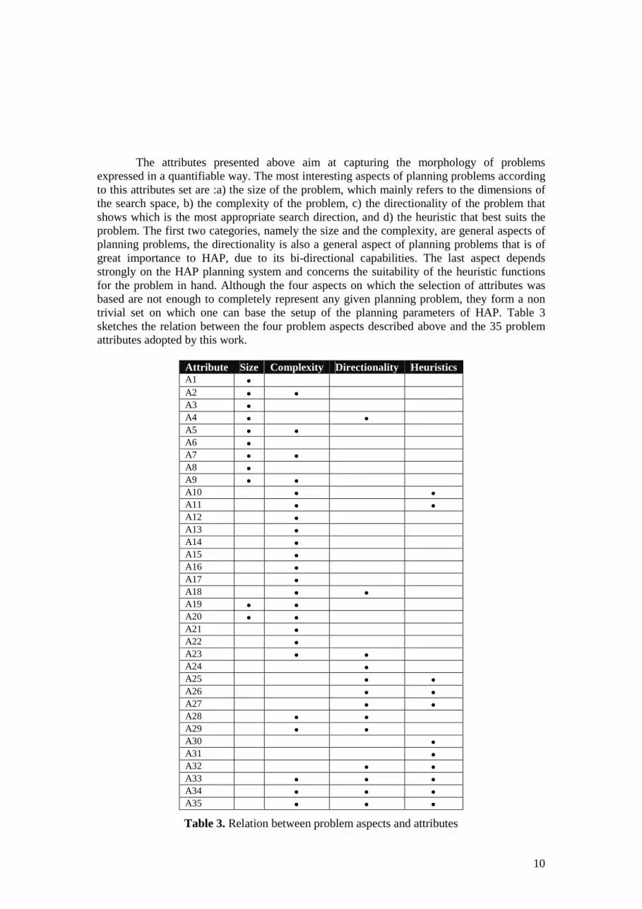
The attributes presented above aim at capturing the morphology of problems expressed in a quantifiable way. The most interesting aspects of planning problems according to this attributes set are :a) the size of the problem, which mainly refers to the dimensions of the search space, b) the complexity of the problem, c) the directionality of the problem that shows which is the most appropriate search direction, and d) the heuristic that best suits the problem. The first two categories, namely the size and the complexity, are general aspects of planning problems, the directionality is also a general aspect of planning problems that is of great importance to HAP, due to its bi-directional capabilities. The last aspect depends strongly on the HAP planning system and concerns the suitability of the heuristic functions for the problem in hand. Although the four aspects on which the selection of attributes was based are not enough to completely represent any given planning problem, they form a non trivial set on which one can base the setup of the planning parameters of HAP. Table 3 sketches the relation between the four problem aspects described above and the 35 problem attributes adopted by this work.

Attribute Size Complexity Directionality Heuristics A1 A2 A3 A4 A5 A6 A7 A8 A9 A10 A11 A12 A13 A14 A15 A16 A17 A18 A19 A20 A21 A22 A23 A24 A25 A26 A27 A28 A29 A30 A31 A32 A33 A34 A35

Table 3. Relation between problem aspects and attributes

11

The initial set of the 35 problem attributes was then processed using machine learning techniques in order to figure out their suitability for the purposes of our work. The outcome of this processing was a reduced set containing 30 attributes, since the other 5 did not seem to play an important role for the planner configuration. The attributes that were filtered out of the set are: A14, A16, A18, A19 and A20. More details about the machine learning technique used for reducing the set of attributes will be given in the following section.

6. Learning Rules

This section describes the steps of our methodology for discovering rules that associates the characteristics of a planning problem with the parameters of HAP.

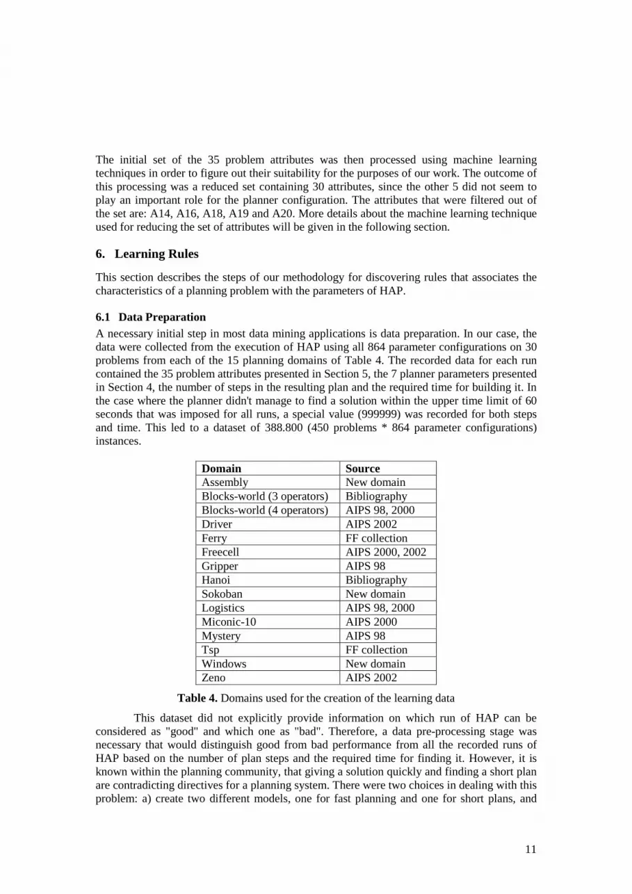
6.1 Data Preparation A necessary initial step in most data mining applications is data preparation. In our case, the data were collected from the execution of HAP using all 864 parameter configurations on 30 problems from each of the 15 planning domains of Table 4. The recorded data for each run contained the 35 problem attributes presented in Section 5, the 7 planner parameters presented in Section 4, the number of steps in the resulting plan and the required time for building it. In the case where the planner didn't manage to find a solution within the upper time limit of 60 seconds that was imposed for all runs, a special value (999999) was recorded for both steps and time. This led to a dataset of 388.800 (450 problems * 864 parameter configurations) instances.

Domain Source Assembly New domain Blocks-world (3 operators) Bibliography Blocks-world (4 operators) AIPS 98, 2000 Driver AIPS 2002 Ferry FF collection Freecell AIPS 2000, 2002 Gripper AIPS 98 Hanoi Bibliography Sokoban New domain Logistics AIPS 98, 2000 Miconic-10 AIPS 2000 Mystery AIPS 98 Tsp FF collection Windows New domain Zeno AIPS 2002

Table 4. Domains used for the creation of the learning data

This dataset did not explicitly provide information on which run of HAP can be considered as "good" and which one as "bad". Therefore, a data pre-processing stage was necessary that would distinguish good from bad performance from all the recorded runs of HAP based on the number of plan steps and the required time for finding it. However, it is known within the planning community, that giving a solution quickly and finding a short plan are contradicting directives for a planning system. There were two choices in dealing with this problem: a) create two different models, one for fast planning and one for short plans, and

12

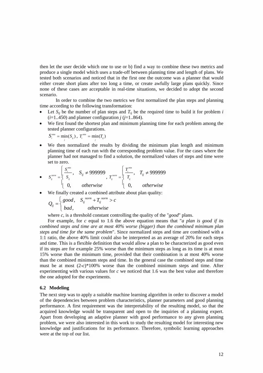
then let the user decide which one to use or b) find a way to combine these two metrics and produce a single model which uses a trade-off between planning time and length of plans. We tested both scenarios and noticed that in the first one the outcome was a planner that would either create short plans after too long a time, or create awfully large plans quickly. Since none of these cases are acceptable in real-time situations, we decided to adopt the second scenario.

In order to combine the two metrics we first normalized the plan steps and planning time according to the following transformation: Let Sij be the number of plan steps and Tij be the required time to build it for problem i

(i=1..450) and planner configuration j (j=1..864). We first found the shortest plan and minimum planning time for each problem among the

tested planner configurations. min min( )i ij

j

SS � , min min( )i ij

j

T T�

We then normalized the results by dividing the minimum plan length and minimum planning time of each run with the corresponding problem value. For the cases where the planner had not managed to find a solution, the normalized values of steps and time were set to zero.

min

, 999999

0,

i

norm

ijij

ij

S

SSS

otherwise

�

���

��

,

min

, 999999

0,

i

norm

ijij

ij

T

TTT

otherwise

�

���

��

We finally created a combined attribute about plan quality:

,

,

norm normij ij

ij

good S T cQ

bad otherwise

� � �� �

where c, is a threshold constant controlling the quality of the "good" plans. For example, for c equal to 1.6 the above equation means that "a plan is good if its

combined steps and time are at most 40% worse (bigger) than the combined minimum plan steps and time for the same problem". Since normalized steps and time are combined with a 1:1 ratio, the above 40% limit could also be interpreted as an average of 20% for each steps and time. This is a flexible definition that would allow a plan to be characterized as good even if its steps are for example 25% worse than the minimum steps as long as its time is at most 15% worse than the minimum time, provided that their combination is at most 40% worse than the combined minimum steps and time. In the general case the combined steps and time must be at most (2-c)*100% worse than the combined minimum steps and time. After experimenting with various values for c we noticed that 1.6 was the best value and therefore the one adopted for the experiments.

6.2 Modeling The next step was to apply a suitable machine learning algorithm in order to discover a model of the dependencies between problem characteristics, planner parameters and good planning performance. A first requirement was the interpretability of the resulting model, so that the acquired knowledge would be transparent and open to the inquiries of a planning expert. Apart from developing an adaptive planner with good performance to any given planning problem, we were also interested in this work to study the resulting model for interesting new knowledge and justifications for its performance. Therefore, symbolic learning approaches were at the top of our list.

13

Mining association rules from the resulting dataset was a first idea, which however was turned down due to the fact that it would produce too many rules making it extremely difficult to produce all the relevant ones. In our previous work (Vrakas et al., 2003), we have used the approach of classification based on association rules (Liu, Hsu & Ma, 1998), which induces association rules that only have a specific target attribute on the right hand side. However, such an approach was proved inappropriate for our current much more extended dataset.

We therefore turned towards classification rule learning approaches, and specifically decided to use the SLIPPER rule learning system (Cohen & Singer, 1999) which is fast, robust, easy to use, and its hypotheses are compact and easy to understand. SLIPPER generates rule sets by repeatedly boosting a simple, greedy rule learner. This learner splits the training data, grows a single rule using one subset of the data and then prunes the rule using the other subset. The metrics that guide the growing and pruning of rules is based on the formal analysis of boosting algorithms. The implementation of SLIPPER that we used handles only two-class classification problems. This suited fine our two-class problem of "good" and "bad" performance. The output of SLIPPER is a weighted rule set, in which each rule R is associated with a confidence CR, where all rules predict membership in only one of the two classes. There is also one default rule that predicts the complementary class in case no rule satisfies the example to be classified.

6.3 Feature Selection The large number of problem attributes (35) together with the comparatively small number of problems (450) raises the known problem of the curse of dimensionality: the higher the dimensionality of the input space, the more data may be needed to discover a good model. We decided to perform feature selection in order to reduce the number of attributes and possibly enhance the resulting model. Feature selection is an interesting research field, with many established approaches especially when it is applied to the task of classification (Dash & Liu, 1997). We here followed an approach similar to the Decision Tree Method (Cardie, 1994). The Decision Tree Method involves running the c4.5 learning algorithm over a set of training examples and selecting the features that appear in the pruned decision tree. We run SLIPPER 15 times on the data of each domain and recorded the frequency of the appearance of the 35 features in the resulting rules and their distribution over the planning parameters. With a careful study on the results we noticed that there were attributes that: a) rarely appeared in the rules, or b) the frequency of their appearance was inconsistent among the 15 models or c) their distribution over the planning parameters was not uniform in the different rule models. These attributes were filtered out because they would either be useless or disorienting for the general models that were the target of our research. The excluded features are: A14, A16, A18, A19 and A20.

SLIPPER was run on the dataset with the 30 retained problem attributes and produced 79 classification rules predicting good plans based on the rest of the attributes and a default rule predicting bad plans.

7. The Rule-Based Planner Tuner

The next step was to embed the learned rules in HAP as a rule-based system that decides the optimal configuration of planning parameters based on the characteristics of a given problem. In order to perform this task certain issues had to be addressed:

14

7.1 Should all the rules be included? The rules that could actually be used for adaptive planning are those that associated, at the same time, problem characteristics, planning parameters and the quality field. So, the first step was to filter out the rules that included only problem characteristics as their antecedents. This process filtered out 21 rules from the initial set of 79 rules. We notice here that there were no rules that included only parameters. If such rules existed, then this would mean that certain parameter values are good regardless of the problem and the corresponding parameters should be fixed.

The remaining 58 rules modeling good performance were subsequently transformed so that only the attributes concerning problem characteristics remained as antecedents and the planning parameters were moved on the right-hand side of the rule as conclusions, omitting the rule quality attribute. In this way, a rule decides one or more planning parameters based on one or more problem characteristics. For example, assume that the following is a rule produced by SLIPPER, where Pi are problem characteristics and Cj are planner parameters:

IF P1 and ... and Pn and C1 and ... and Cm THEN good

If we interpret this rule as a backward chaining rule, then in order to achieve good performance it suffices to have all Pi problem characteristics and all Cj planner parameters. If all the problem characteristics Pi are met, then the only way to achieve good performance (using this rule) is to set the Cj planner parameters. This can be interpreted as a production (forward chaining) rule having all Pi at the rule condition and all Cj at the rule action:

IF P1 and ... and Pn THEN C1 and ... and Cm

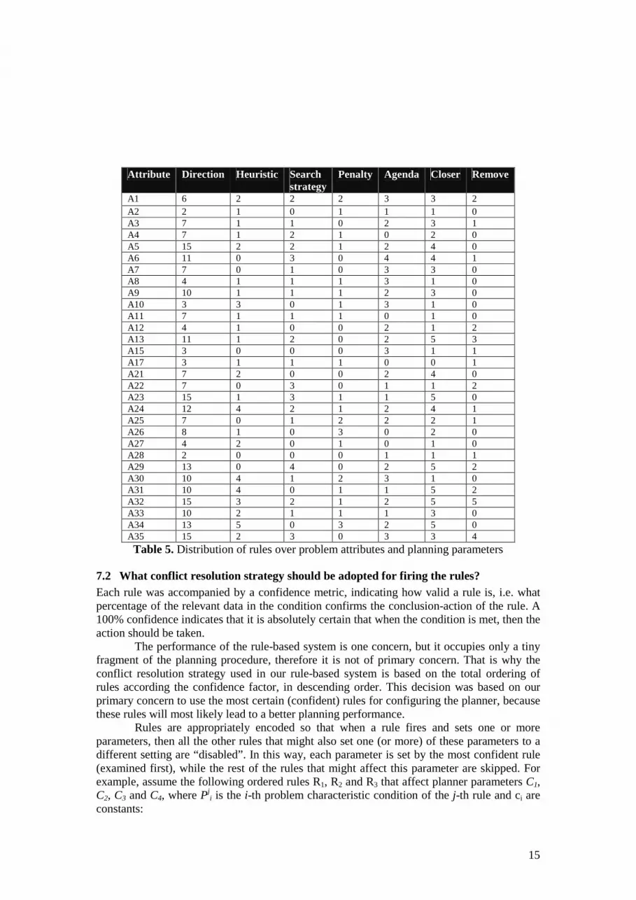
We notice here that the conditions of rules produced by SLIPPER are not mutually exclusive and may cover common data sets; therefore, the production rules generated using the above transformation are disjunctive and can be fired independently from each other. For any given problem several rules may simultaneously apply. The conflict resolution strategy used is discussed in the next subsection. Table 5 outlines the distribution of rules over the 30 problem attributes and the planning parameters. The number in a cell Cij refer to the number of rules associating the attribute in line i with the parameter in column j. Comparing Table 5 with Table 3 we can conclude that the learned model contains information that seems reasonable, for example we expected the direction to depend on attributes A4 (number of initial facts divided by the number of goal facts), A23 (ratio of the relaxed branching factors) or A24 (ratio of the branching factors), and there are also associations that support our claim that there are hidden dynamics in problems which cannot be easily investigated. For example, there is no obvious connection between the search direction and the average number of actions per fact (attribute A5), nevertheless there are 15 rules that associate them.

15

Attribute Direction Heuristic Search

strategy Penalty Agenda Closer Remove

A1 6 2 2 2 3 3 2 A2 2 1 0 1 1 1 0 A3 7 1 1 0 2 3 1 A4 7 1 2 1 0 2 0 A5 15 2 2 1 2 4 0 A6 11 0 3 0 4 4 1 A7 7 0 1 0 3 3 0 A8 4 1 1 1 3 1 0 A9 10 1 1 1 2 3 0 A10 3 3 0 1 3 1 0 A11 7 1 1 1 0 1 0 A12 4 1 0 0 2 1 2 A13 11 1 2 0 2 5 3 A15 3 0 0 0 3 1 1 A17 3 1 1 1 0 0 1 A21 7 2 0 0 2 4 0 A22 7 0 3 0 1 1 2 A23 15 1 3 1 1 5 0 A24 12 4 2 1 2 4 1 A25 7 0 1 2 2 2 1 A26 8 1 0 3 0 2 0 A27 4 2 0 1 0 1 0 A28 2 0 0 0 1 1 1 A29 13 0 4 0 2 5 2 A30 10 4 1 2 3 1 0 A31 10 4 0 1 1 5 2 A32 15 3 2 1 2 5 5 A33 10 2 1 1 1 3 0 A34 13 5 0 3 2 5 0 A35 15 2 3 0 3 3 4

Table 5. Distribution of rules over problem attributes and planning parameters

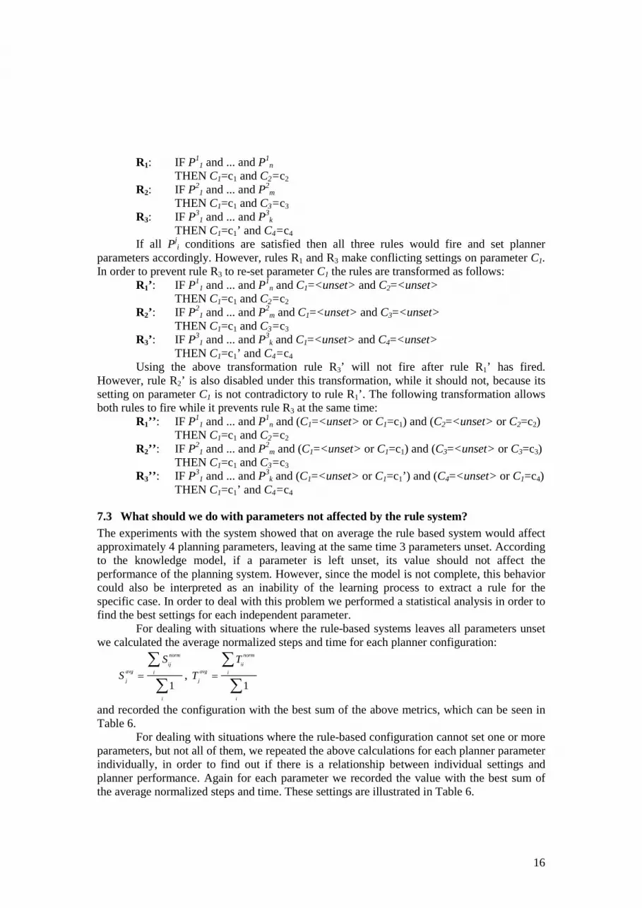
7.2 What conflict resolution strategy should be adopted for firing the rules? Each rule was accompanied by a confidence metric, indicating how valid a rule is, i.e. what percentage of the relevant data in the condition confirms the conclusion-action of the rule. A 100% confidence indicates that it is absolutely certain that when the condition is met, then the action should be taken. The performance of the rule-based system is one concern, but it occupies only a tiny fragment of the planning procedure, therefore it is not of primary concern. That is why the conflict resolution strategy used in our rule-based system is based on the total ordering of rules according the confidence factor, in descending order. This decision was based on our primary concern to use the most certain (confident) rules for configuring the planner, because these rules will most likely lead to a better planning performance. Rules are appropriately encoded so that when a rule fires and sets one or more parameters, then all the other rules that might also set one (or more) of these parameters to a different setting are “disabled”. In this way, each parameter is set by the most confident rule (examined first), while the rest of the rules that might affect this parameter are skipped. For example, assume the following ordered rules R1, R2 and R3 that affect planner parameters C1, C2, C3 and C4, where Pj

i is the i-th problem characteristic condition of the j-th rule and ci are constants:

16

R1: IF P11 and ... and P1

n THEN C1=c1 and C2=c2 R2: IF P2

1 and ... and P2m

THEN C1=c1 and C3=c3 R3: IF P3

1 and ... and P3k

THEN C1=c1’ and C4=c4 If all Pj

i conditions are satisfied then all three rules would fire and set planner parameters accordingly. However, rules R1 and R3 make conflicting settings on parameter C1. In order to prevent rule R3 to re-set parameter C1 the rules are transformed as follows: R1’ : IF P1

1 and ... and P1n and C1=<unset> and C2=<unset>

THEN C1=c1 and C2=c2 R2’ : IF P2

1 and ... and P2m and C1=<unset> and C3=<unset>

THEN C1=c1 and C3=c3 R3’ : IF P3

1 and ... and P3k and C1=<unset> and C4=<unset>

THEN C1=c1’ and C4=c4 Using the above transformation rule R3’ will not fire after rule R1’ has fired. However, rule R2’ is also disabled under this transformation, while it should not, because its setting on parameter C1 is not contradictory to rule R1’. The following transformation allows both rules to fire while it prevents rule R3 at the same time: R1’’ : IF P1

1 and ... and P1n and (C1=<unset> or C1=c1) and (C2=<unset> or C2=c2)

THEN C1=c1 and C2=c2 R2’’ : IF P2

1 and ... and P2m and (C1=<unset> or C1=c1) and (C3=<unset> or C3=c3)

THEN C1=c1 and C3=c3 R3’’ : IF P3

1 and ... and P3k and (C1=<unset> or C1=c1’) and (C4=<unset> or C1=c4)

THEN C1=c1’ and C4=c4

7.3 What should we do with parameters not affected by the rule system? The experiments with the system showed that on average the rule based system would affect approximately 4 planning parameters, leaving at the same time 3 parameters unset. According to the knowledge model, if a parameter is left unset, its value should not affect the performance of the planning system. However, since the model is not complete, this behavior could also be interpreted as an inability of the learning process to extract a rule for the specific case. In order to deal with this problem we performed a statistical analysis in order to find the best settings for each independent parameter. For dealing with situations where the rule-based systems leaves all parameters unset we calculated the average normalized steps and time for each planner configuration:

1

norm

ijavg i

j

i

S

S �

,

1

norm

iiavg i

j

i

T

T �

and recorded the configuration with the best sum of the above metrics, which can be seen in Table 6. For dealing with situations where the rule-based configuration cannot set one or more parameters, but not all of them, we repeated the above calculations for each planner parameter individually, in order to find out if there is a relationship between individual settings and planner performance. Again for each parameter we recorded the value with the best sum of the average normalized steps and time. These settings are illustrated in Table 6.

17

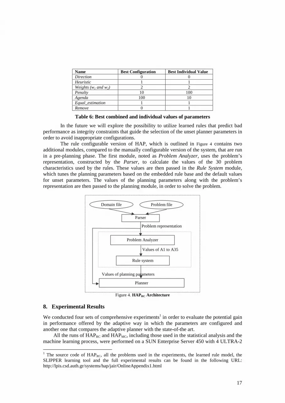
Name Best Configuration Best Individual Value Direction 0 0 Heuristic 1 1 Weights (w1 and w2) 2 2 Penalty 10 100 Agenda 100 10 Equal_estimation 1 1 Remove 0 1

Table 6: Best combined and individual values of parameters

In the future we will explore the possibility to utilize learned rules that predict bad performance as integrity constraints that guide the selection of the unset planner parameters in order to avoid inappropriate configurations.

The rule configurable version of HAP, which is outlined in Figure 4 contains two additional modules, compared to the manually configurable version of the system, that are run in a pre-planning phase. The first module, noted as Problem Analyzer, uses the problem’s representation, constructed by the Parser, to calculate the values of the 30 problem characteristics used by the rules. These values are then passed in the Rule System module, which tunes the planning parameters based on the embedded rule base and the default values for unset parameters. The values of the planning parameters along with the problem’s representation are then passed to the planning module, in order to solve the problem.

Figure 4. HAPRC Architecture

8. Experimental Results

We conducted four sets of comprehensive experiments1 in order to evaluate the potential gain in performance offered by the adaptive way in which the parameters are configured and another one that compares the adaptive planner with the state-of-the art.

All the runs of HAPRC and HAPMC, including those used in the statistical analysis and the machine learning process, were performed on a SUN Enterprise Server 450 with 4 ULTRA-2

1 The source code of HAPRC, all the problems used in the experiments, the learned rule model, the SLIPPER learning tool and the full experimental results can be found in the following URL: http://lpis.csd.auth.gr/systems/hap/jair/OnlineAppendix1.html

Problem file Domain file

Parser

Problem Analyzer

Rule system

Planner

Problem representation

Values of A1 to A35

Values of planning parameters

18

processors at 400 MHz and 2 GB of shared memory. The Operating system of the computer was SUN Solaris 8. For all experiments we counted CPU clocks and we had an upper limit of 60 sec, beyond which the planner would stop and report that the problem is unsolvable.

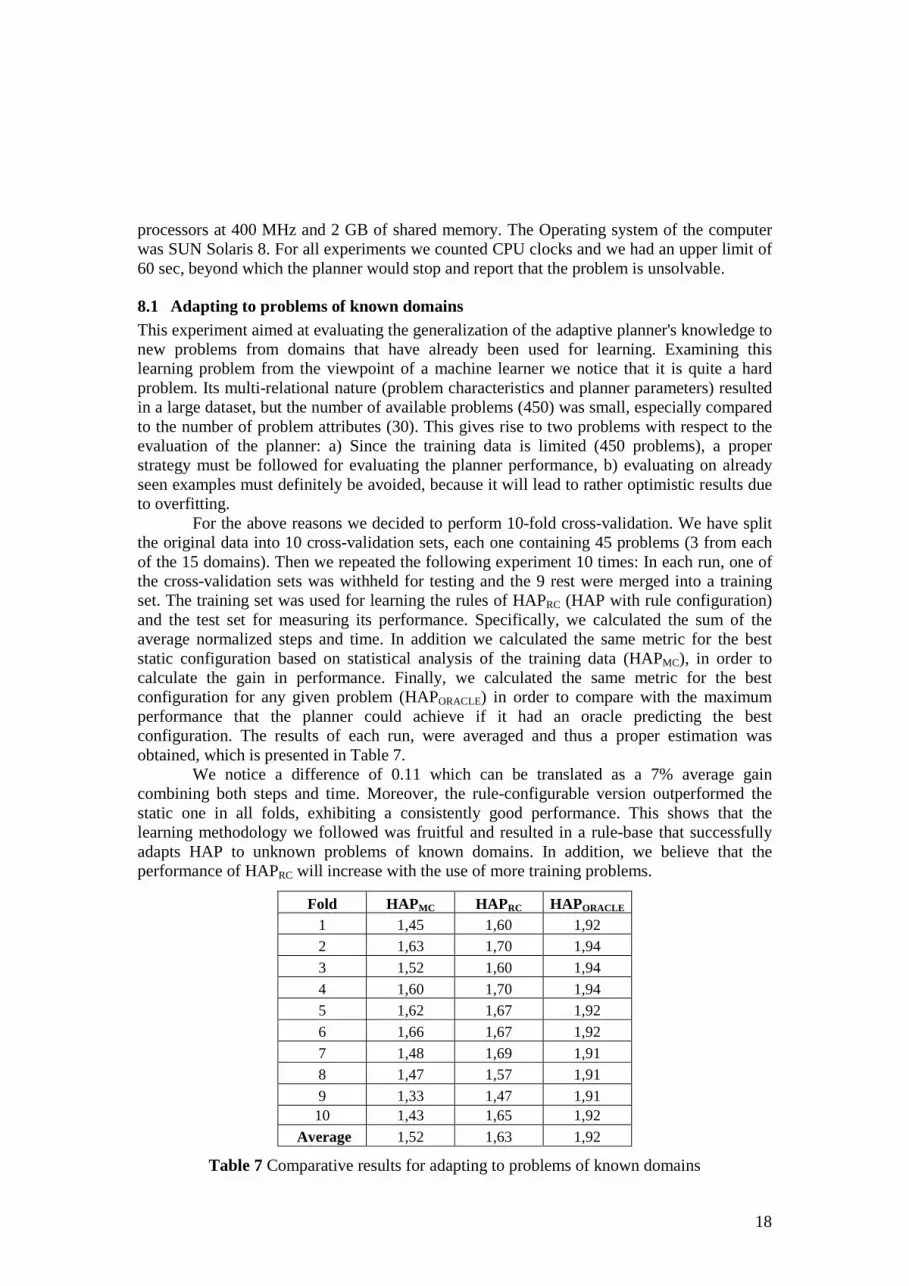
8.1 Adapting to problems of known domains This experiment aimed at evaluating the generalization of the adaptive planner's knowledge to new problems from domains that have already been used for learning. Examining this learning problem from the viewpoint of a machine learner we notice that it is quite a hard problem. Its multi-relational nature (problem characteristics and planner parameters) resulted in a large dataset, but the number of available problems (450) was small, especially compared to the number of problem attributes (30). This gives rise to two problems with respect to the evaluation of the planner: a) Since the training data is limited (450 problems), a proper strategy must be followed for evaluating the planner performance, b) evaluating on already seen examples must definitely be avoided, because it will lead to rather optimistic results due to overfitting. For the above reasons we decided to perform 10-fold cross-validation. We have split the original data into 10 cross-validation sets, each one containing 45 problems (3 from each of the 15 domains). Then we repeated the following experiment 10 times: In each run, one of the cross-validation sets was withheld for testing and the 9 rest were merged into a training set. The training set was used for learning the rules of HAPRC (HAP with rule configuration) and the test set for measuring its performance. Specifically, we calculated the sum of the average normalized steps and time. In addition we calculated the same metric for the best static configuration based on statistical analysis of the training data (HAPMC), in order to calculate the gain in performance. Finally, we calculated the same metric for the best configuration for any given problem (HAPORACLE) in order to compare with the maximum performance that the planner could achieve if it had an oracle predicting the best configuration. The results of each run, were averaged and thus a proper estimation was obtained, which is presented in Table 7.

We notice a difference of 0.11 which can be translated as a 7% average gain combining both steps and time. Moreover, the rule-configurable version outperformed the static one in all folds, exhibiting a consistently good performance. This shows that the learning methodology we followed was fruitful and resulted in a rule-base that successfully adapts HAP to unknown problems of known domains. In addition, we believe that the performance of HAPRC will increase with the use of more training problems.

Fold HAPMC HAPRC HAPORACLE 1 1,45 1,60 1,92 2 1,63 1,70 1,94

3 1,52 1,60 1,94

4 1,60 1,70 1,94 5 1,62 1,67 1,92

6 1,66 1,67 1,92

7 1,48 1,69 1,91 8 1,47 1,57 1,91

9 1,33 1,47 1,91 10 1,43 1,65 1,92

Average 1,52 1,63 1,92

Table 7 Comparative results for adapting to problems of known domains

19

8.2 Adapting to problems of unknown domains The second experiment aimed at evaluating the generalization of the adaptive planner's knowledge to problems of new domains that have not been used for learning before. In a sense this would give an estimation for the behavior of the planner when confronted with a previously unknown problem of a new domain.

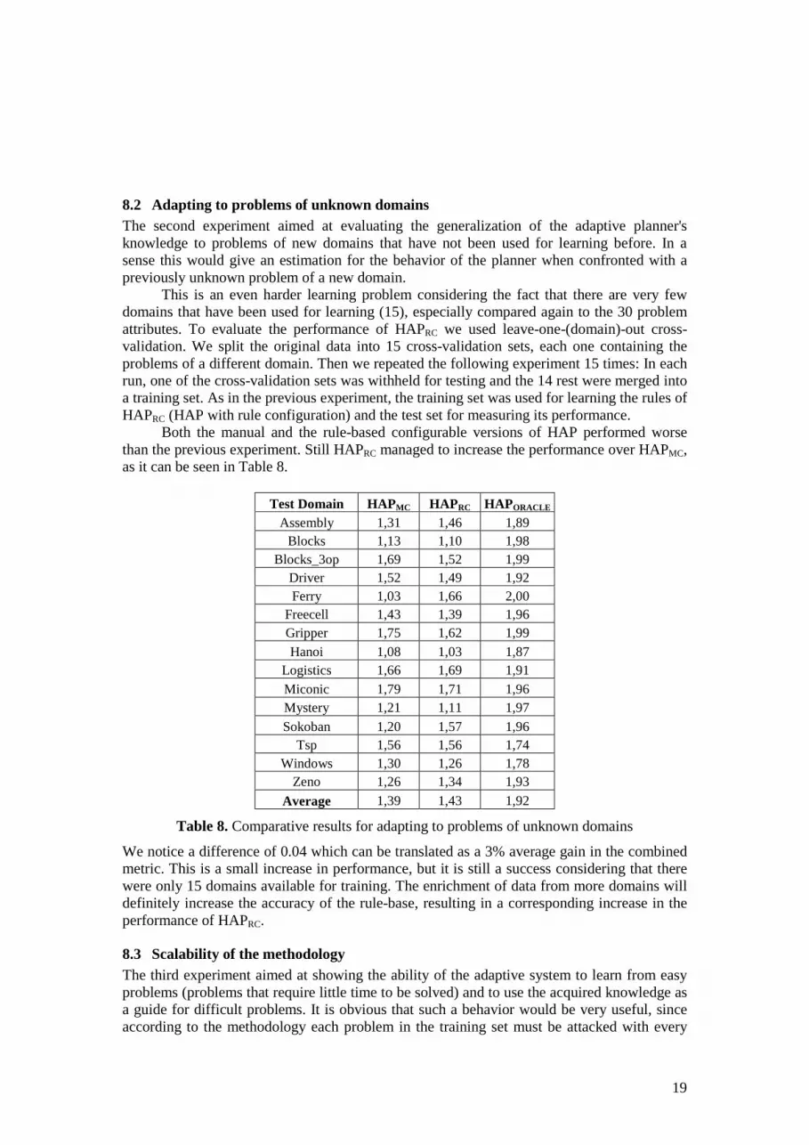
This is an even harder learning problem considering the fact that there are very few domains that have been used for learning (15), especially compared again to the 30 problem attributes. To evaluate the performance of HAPRC we used leave-one-(domain)-out cross-validation. We split the original data into 15 cross-validation sets, each one containing the problems of a different domain. Then we repeated the following experiment 15 times: In each run, one of the cross-validation sets was withheld for testing and the 14 rest were merged into a training set. As in the previous experiment, the training set was used for learning the rules of HAPRC (HAP with rule configuration) and the test set for measuring its performance.

Both the manual and the rule-based configurable versions of HAP performed worse than the previous experiment. Still HAPRC managed to increase the performance over HAPMC, as it can be seen in Table 8.

Test Domain HAPMC HAPRC HAPORACLE

Assembly 1,31 1,46 1,89 Blocks 1,13 1,10 1,98

Blocks_3op 1,69 1,52 1,99 Driver 1,52 1,49 1,92 Ferry 1,03 1,66 2,00

Freecell 1,43 1,39 1,96 Gripper 1,75 1,62 1,99 Hanoi 1,08 1,03 1,87

Logistics 1,66 1,69 1,91 Miconic 1,79 1,71 1,96 Mystery 1,21 1,11 1,97

Sokoban 1,20 1,57 1,96 Tsp 1,56 1,56 1,74

Windows 1,30 1,26 1,78 Zeno 1,26 1,34 1,93

Average 1,39 1,43 1,92

Table 8. Comparative results for adapting to problems of unknown domains

We notice a difference of 0.04 which can be translated as a 3% average gain in the combined metric. This is a small increase in performance, but it is still a success considering that there were only 15 domains available for training. The enrichment of data from more domains will definitely increase the accuracy of the rule-base, resulting in a corresponding increase in the performance of HAPRC.

8.3 Scalability of the methodology The third experiment aimed at showing the ability of the adaptive system to learn from easy problems (problems that require little time to be solved) and to use the acquired knowledge as a guide for difficult problems. It is obvious that such a behavior would be very useful, since according to the methodology each problem in the training set must be attacked with every

20

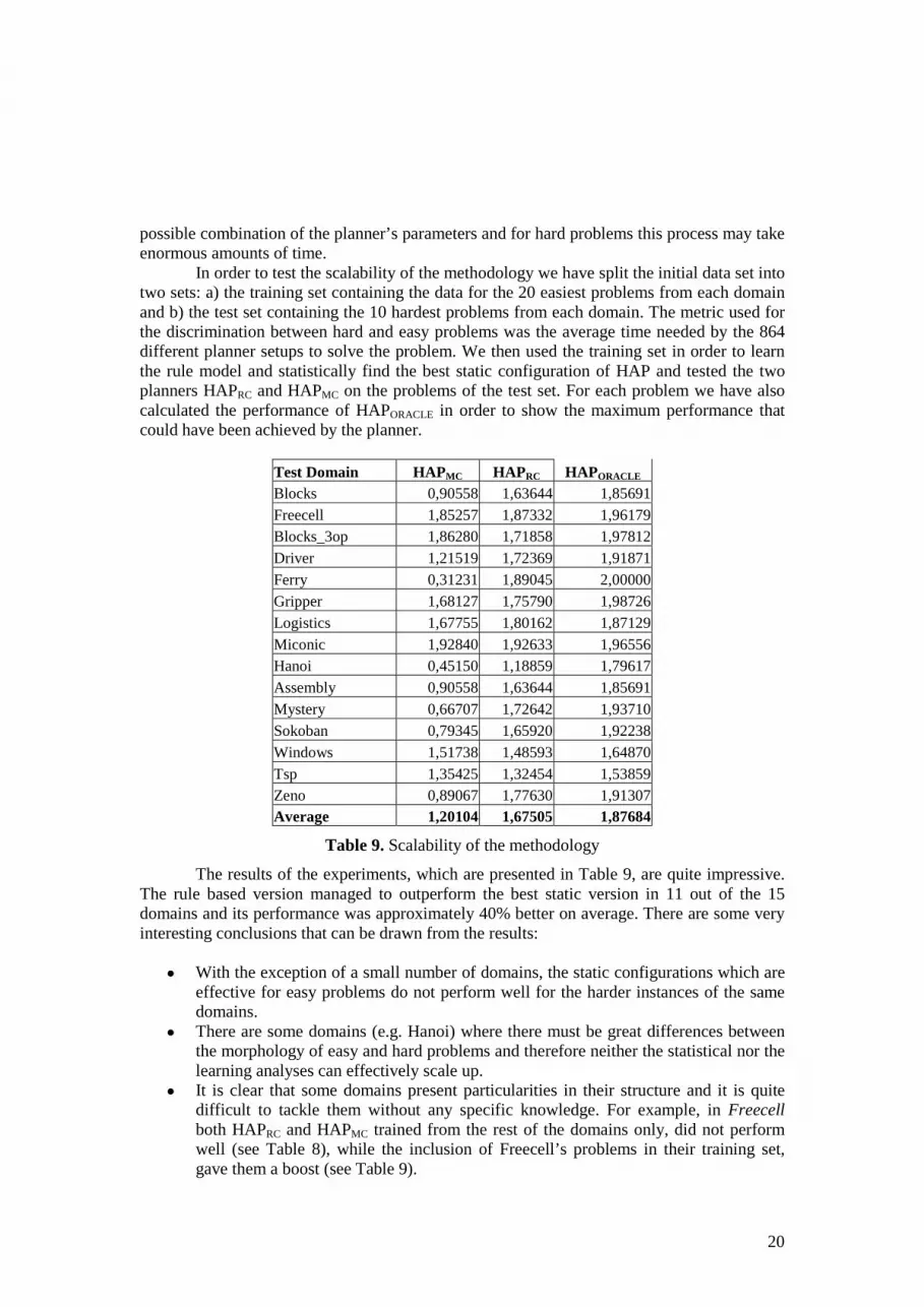
possible combination of the planner’s parameters and for hard problems this process may take enormous amounts of time. In order to test the scalability of the methodology we have split the initial data set into two sets: a) the training set containing the data for the 20 easiest problems from each domain and b) the test set containing the 10 hardest problems from each domain. The metric used for the discrimination between hard and easy problems was the average time needed by the 864 different planner setups to solve the problem. We then used the training set in order to learn the rule model and statistically find the best static configuration of HAP and tested the two planners HAPRC and HAPMC on the problems of the test set. For each problem we have also calculated the performance of HAPORACLE in order to show the maximum performance that could have been achieved by the planner.

Test Domain HAPMC HAPRC HAPORACLE Blocks 0,90558 1,63644 1,85691 Freecell 1,85257 1,87332 1,96179 Blocks_3op 1,86280 1,71858 1,97812 Driver 1,21519 1,72369 1,91871 Ferry 0,31231 1,89045 2,00000 Gripper 1,68127 1,75790 1,98726 Logistics 1,67755 1,80162 1,87129 Miconic 1,92840 1,92633 1,96556 Hanoi 0,45150 1,18859 1,79617 Assembly 0,90558 1,63644 1,85691 Mystery 0,66707 1,72642 1,93710 Sokoban 0,79345 1,65920 1,92238 Windows 1,51738 1,48593 1,64870 Tsp 1,35425 1,32454 1,53859 Zeno 0,89067 1,77630 1,91307 Average 1,20104 1,67505 1,87684

Table 9. Scalability of the methodology

The results of the experiments, which are presented in Table 9, are quite impressive. The rule based version managed to outperform the best static version in 11 out of the 15 domains and its performance was approximately 40% better on average. There are some very interesting conclusions that can be drawn from the results:

With the exception of a small number of domains, the static configurations which are effective for easy problems do not perform well for the harder instances of the same domains.

There are some domains (e.g. Hanoi) where there must be great differences between the morphology of easy and hard problems and therefore neither the statistical nor the learning analyses can effectively scale up.

It is clear that some domains present particularities in their structure and it is quite difficult to tackle them without any specific knowledge. For example, in Freecell both HAPRC and HAPMC trained from the rest of the domains only, did not perform well (see Table 8), while the inclusion of Freecell’s problems in their training set, gave them a boost (see Table 9).

21

There are domains where there is a clear trade-off between short plans and small planning time. For example, the low performance of HAPORACLE in the Tsp domain shows that the configurations that result in short plans require a lot of planning time and the ones that solve the problems quickly produce bad plans.

The proposed learning paradigm can scale up very well and the main reason for this is the general nature of the selected problem attributes.

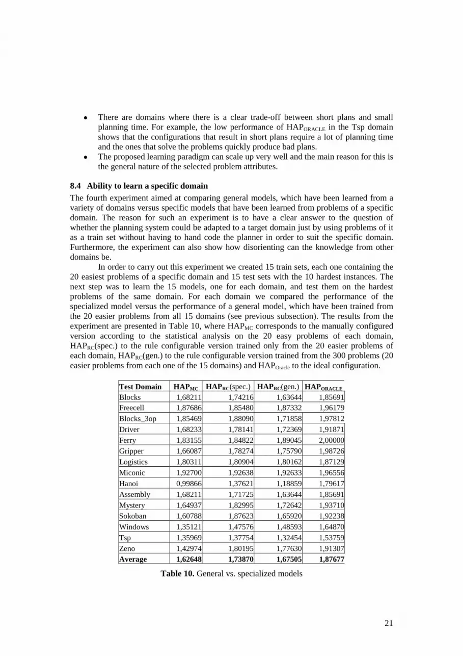
8.4 Ability to learn a specific domain The fourth experiment aimed at comparing general models, which have been learned from a variety of domains versus specific models that have been learned from problems of a specific domain. The reason for such an experiment is to have a clear answer to the question of whether the planning system could be adapted to a target domain just by using problems of it as a train set without having to hand code the planner in order to suit the specific domain. Furthermore, the experiment can also show how disorienting can the knowledge from other domains be.

In order to carry out this experiment we created 15 train sets, each one containing the 20 easiest problems of a specific domain and 15 test sets with the 10 hardest instances. The next step was to learn the 15 models, one for each domain, and test them on the hardest problems of the same domain. For each domain we compared the performance of the specialized model versus the performance of a general model, which have been trained from the 20 easier problems from all 15 domains (see previous subsection). The results from the experiment are presented in Table 10, where HAPMC corresponds to the manually configured version according to the statistical analysis on the 20 easy problems of each domain, HAPRC(spec.) to the rule configurable version trained only from the 20 easier problems of each domain, HAPRC(gen.) to the rule configurable version trained from the 300 problems (20 easier problems from each one of the 15 domains) and HAPOracle to the ideal configuration.

Test Domain HAPMC HAPRC(spec.) HAPRC(gen.) HAPORACLE Blocks 1,68211 1,74216 1,63644 1,85691Freecell 1,87686 1,85480 1,87332 1,96179Blocks_3op 1,85469 1,88090 1,71858 1,97812Driver 1,68233 1,78141 1,72369 1,91871Ferry 1,83155 1,84822 1,89045 2,00000Gripper 1,66087 1,78274 1,75790 1,98726Logistics 1,80311 1,80904 1,80162 1,87129Miconic 1,92700 1,92638 1,92633 1,96556Hanoi 0,99866 1,37621 1,18859 1,79617Assembly 1,68211 1,71725 1,63644 1,85691Mystery 1,64937 1,82995 1,72642 1,93710Sokoban 1,60788 1,87623 1,65920 1,92238Windows 1,35121 1,47576 1,48593 1,64870Tsp 1,35969 1,37754 1,32454 1,53759Zeno 1,42974 1,80195 1,77630 1,91307Average 1,62648 1,73870 1,67505 1,87677

Table 10. General vs. specialized models

22

According to the results presented in Table 10, the machine learning powered version outperforms the best static one in 13 out of the 15 domains and on average it is approximately 7% better. This shows that we can also induce efficient models that perform well in difficult problems of a given domain when trained on easy problems of this domain only.

Comparing the specialized model with the general one, we see that it is on average 4% better. This shows that in order to adapt to a single domain, it is better to train the planner exclusively from problems of that domain. However, such an approach would compromise the generality of the adaptive planner.

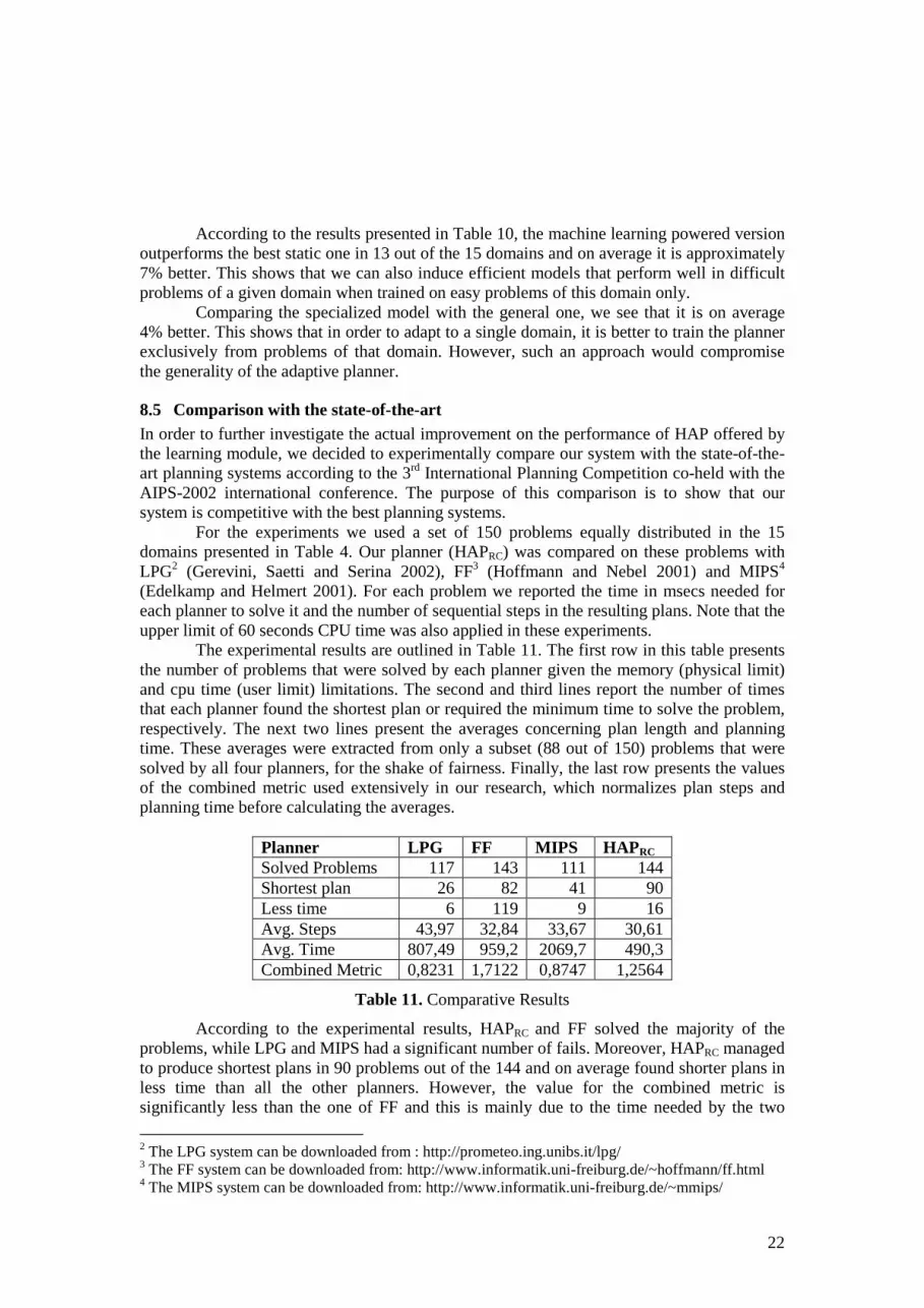
8.5 Comparison with the state-of-the-art In order to further investigate the actual improvement on the performance of HAP offered by the learning module, we decided to experimentally compare our system with the state-of-the-art planning systems according to the 3rd International Planning Competition co-held with the AIPS-2002 international conference. The purpose of this comparison is to show that our system is competitive with the best planning systems. For the experiments we used a set of 150 problems equally distributed in the 15 domains presented in Table 4. Our planner (HAPRC) was compared on these problems with LPG2 (Gerevini, Saetti and Serina 2002), FF3 (Hoffmann and Nebel 2001) and MIPS4 (Edelkamp and Helmert 2001). For each problem we reported the time in msecs needed for each planner to solve it and the number of sequential steps in the resulting plans. Note that the upper limit of 60 seconds CPU time was also applied in these experiments. The experimental results are outlined in Table 11. The first row in this table presents the number of problems that were solved by each planner given the memory (physical limit) and cpu time (user limit) limitations. The second and third lines report the number of times that each planner found the shortest plan or required the minimum time to solve the problem, respectively. The next two lines present the averages concerning plan length and planning time. These averages were extracted from only a subset (88 out of 150) problems that were solved by all four planners, for the shake of fairness. Finally, the last row presents the values of the combined metric used extensively in our research, which normalizes plan steps and planning time before calculating the averages.

Planner LPG FF MIPS HAPRC Solved Problems 117 143 111 144 Shortest plan 26 82 41 90 Less time 6 119 9 16 Avg. Steps 43,97 32,84 33,67 30,61 Avg. Time 807,49 959,2 2069,7 490,3 Combined Metric 0,8231 1,7122 0,8747 1,2564

Table 11. Comparative Results

According to the experimental results, HAPRC and FF solved the majority of the problems, while LPG and MIPS had a significant number of fails. Moreover, HAPRC managed to produce shortest plans in 90 problems out of the 144 and on average found shorter plans in less time than all the other planners. However, the value for the combined metric is significantly less than the one of FF and this is mainly due to the time needed by the two

2 The LPG system can be downloaded from : http://prometeo.ing.unibs.it/lpg/ 3 The FF system can be downloaded from: http://www.informatik.uni-freiburg.de/~hoffmann/ff.html 4 The MIPS system can be downloaded from: http://www.informatik.uni-freiburg.de/~mmips/

23

planners to solve the problems. Although FF was faster than HAPRC in the vast majority of the problems and this is clear from Table 11, since FF took less time than any planner in 119 problems, in some of the remaining problems FF needed extremely large amount of time to solve them. These negative peaks in the performance of FF, concerning planning time, are responsible for the large average time. Our metric however, manages to smooth these peaks due to normalization and the resulting combined metric comparison is quite different. Concluding, HAPRC seems to be at least a fair match to three of the best domain independent planners, generally producing shorter plans and exhibiting a more stable performance.

9. Conclusions and Future Work

This paper presented our research work in the area of using Machine Learning and Rule-based techniques in order to infer and utilize domain knowledge in Automated Planning. The learned knowledge consists of rules that associate specific values or value ranges of measurable problem attributes with the best values for one or more planning parameter, such as the direction of search or the heuristic function. The knowledge is learned offline and it is embedded in a rule system, which is utilized by the planner in a pre-processing phase in order to decide for the best setup of the planner according to the values of the given problem attributes.

In order to extract these rules, we experimented with all possible combinations of the values of the planning parameters of an adjustable planning system called HAP, over 450 problems of 15 domains. For each run we recorded the values of the problem attributes, the values of the planning parameters and the performance of the planner (in terms of planning time and plan length). The two performance metrics were then normalized and combined in a single one. The next step was to apply a criterion on the performance metric in order to specify whether a run is considered to be good or bad. This yielded a very large dataset of approximately 389,000 records, containing the values of the problem attributes, the values of the planning parameters and a Boolean field for performance. The dataset was then fed in a machine learning tool in order to learn rules associating good performance with planning parameters and problem attributes. The classification rules were then transformed into production rules that tune planner parameters in the presence of certain problem characteristics and were embedded in the planner. The whole system was thoroughly tested using various experiments and according to the results managed to offer a significant increase in the performance of the planner.

The experimental results, presented in the paper, have shown that the adaptive planning system performs on average better than any statistically found static configuration. The speedup improves significantly, when the system is tested on unseen problems of known domains, even when the knowledge was induced by far easier problems than the tested ones. Such a behavior can prove very useful in customizing domain independent planners for specific domains using only a small number of easy-to-solve problems for training, when it cannot be afforded to reprogram the planning system.

The speedup of our approach compared to the statistically found best configuration can be attributed to the fact that it treats planner parameters as associations of the problem characteristics, whereas the statistical analysis tries to associate planner performance with planner settings, ignoring the problem morphology. In the future we plan to expand the application of Machine Learning to include more measurable problem characteristics in order to come up with vectors of values that represent the problems in a unique way and manage to capture all the hidden dynamics. We also plan to add more configurable parameters of planning, such as parameters for time and resource

24

handling and enrich the HAP system with other heuristics from state-of-the-art planning systems. In addition, we will explore the applicability of different rule-learning algorithms, such as decision-tree learning that could potentially provide knowledge of better quality. We will also investigate the use of alternative automatic feature selection techniques that could prune the vector of input attributes thus giving the learning algorithm the ability to achieve better results. The interpretability of the resulting model and its analysis by planning experts will also be a point of greater focus in the future.

10. References

Ambite, J. L., Knoblock, C., & Minton, S. (2000). Learning Plan Rewriting Rules. In Proceedings of the 5th International Conference on Artificial Intelligence Planning and Scheduling Systems.

Borrajo, D., & Veloso, M. (1996). Lazy Incremental Learning of Control Knowledge for Efficiently Obtaining Quality Plans. Artificial Intelligence Review,10, 1-34.

Carbonell, J., Knoblock, C., & Minton, S. (1991). PRODIGY: An integrated architecture for planning and learning, in: K. VanLehn, ed., Architectures for Intelligence. Lawrence Erlbaum Associates, 241-278.

Cardie, C. (1994). Using decision trees to improve case-based learning. In Proceedings of Tenth International Conference on Machine Learning, Morgan Kaufmann, New Brunswick, New Jersey, 28-36. Cohen, W., & Singer, Y. (1999). A Simple, Fast, and Effective Rule Learner. In Proceedings of the 16th National Conference on Artificial Intelligence. Dash, M., & Liu, H. (1997). Feature Selection for Classification. Intelligent Data Analysis, 1(3), 131-156.

Edelkamp, S., & Helmert, M. (2001). The Model Checking Integrated Planning System. AI-Magazine, Fall, 67-71. Etzioni, O. (1993). Acquiring Search-Control Knowledge via Static Analysis. Artificial Intelligence 62 (2). 265-301.

Gerevini, A., Saetti, A. & Serina, I. (2003). Planning through Stochastic Local Search and Temporal Action Graphs, to appear in Journal of Artificial Intelligence Research (JAIR).

Gopal, K. (2000). An Adaptive Planner based on Learning of Planning Performance. Master Thesis, Office of Graduate Studies, Texas A&M University.

Hammond, K. (1989). Case-Based Planning: Viewing Planning as a Memory Task. Academic Press, Boston, MA.

25

Hoffmann, J., & Nebel, B. (2001). The FF Planning System: Fast Plan Generation Through Heuristic Search. Journal of Artificial Intelligence Research, 14, 253 – 302.

Howe, A., & Dahlman, E. (1993). A critical assessment of Benchmark comparison in Planning. Journal of Artificial Intelligence Research, 1, 1-15.

Howe, A., Dahlman, E., Hansen, C., vonMayrhauser, A., & Scheetz, M. (1999). Exploiting Competitive Planner Performance. In Proceedings of the 5th European Conference on Planning.

Kambhampati, S., & Hendler, H. (1992). A Validation-Structure-Based Theory of Plan Modification and Reuse. Artificial Intelligence, 55, 193-258.

Knoblock, C. (1990). Learning Abstraction Hierarchies for Problem Solving. In Proceedings of the 8th National Conference on Artificial Intelligence. Menlo Park, California AAAI Press, 923-928.

Liu, B., Hsu, W., & Ma, Y. (1998). Integrating Classification and Association Rule Mining. In Proceedings of the 4th International Conference on Knowledge Discovery and Data Mining (Plenary Presentation).

Martin, M., & Geffner, H. (2000). Learning Generalized Policies in Planning Using Concept Languages. In Proceedings of the 7th International Conference on Knowledge Representation and Reasoning. San Francisco, California, Morgan Kaufmann, 667-677.

Minton, S., (1996). Automatically Configuring Constraint Satisfaction Programs: A Case Study. Constraints 1(1/2), 7-43.

Sutton, R. (1990). Integrated Architectures for learning, planning and reacting based on approximating dynamic programming. In Proceedings of the 7th International Conference on Machine Learning, Austin, Texas. Morgan Kaufmann. 216-224.

Veloso, M., Carbonell, J., Perez, A., Borrajo, D., Fink, E., & Blythe, J. (1995). Integrating planning and learning: The prodigy architecture. Journal of Experimental and Theoretical Artificial Intelligence 7(1), 81-120.

Vrakas, D., & Vlahavas, I., (2001). Combining progression and regression in state-space heuristic planning. In Proceedings of the 6th European Conference on Planning.

Vrakas, D. & Vlahavas, I. (2002). A heuristic for planning based on action evaluation. In Proceedings of the 10th International Conference on Artificial Intelligence: Methodology, Systems and Applications.

26

Vrakas, D., Tsoumakas, G., Bassiliades, N., & Vlahavas, I., (2003). Learning rules for Adaptive Planning. In Proceedings of the 13th International Conference on Automated Planning and Scheduling. Trento, Italy. 82-91. Wang, X., (1996). A Multistrategy Learning System for Planning Operator Acquisition. In Proceedings of the 3rd International Workshop on Multistrategy Learning. Harpers Ferry, West Virginia, 23-25. Zimmerman, T., & Kambhampati, S., (2003). Learning-Assisted Automated Planning: Looking Back, Taking Stock, Going Forward. AI Magazine 24(2), 73-96.