1

Robotic Inspection and 3D GPR-basedReconstruction for Underground Utilities

Jinglun Feng1, Liang Yang1, Jiang Biao2, Jizhong Xiao1∗ Senior Member, IEEE

Abstract—Ground Penetrating Radar (GPR) is an effectivenon-destructive evaluation (NDE) device for inspecting and sur-veying subsurface objects (i.e., rebars, utility pipes) in complexenvironments. However, the current practice for GPR datacollection requires a human inspector to move a GPR cartalong pre-marked grid lines and record the GPR data in bothX and Y directions for post-processing by 3D GPR imagingsoftware. It is a time-consuming and tedious work to surveya large area. Furthermore, identifying the subsurface targetsdepends on the knowledge of an experienced engineer, who has tomake manual and subjective interpretation that limits the GPRapplications, especially in large-scale scenarios. In addition, thecurrent GPR imaging technology is not intuitive, and not fornormal users to understand, and not friendly to visualize. Toaddress the above challenges, this paper presents a novel roboticsystem to collect GPR data, interpret GPR data, localize theunderground utilities, reconstruct and visualize the undergroundobjects’ dense point cloud model in a user-friendly manner. Thissystem is composed of three modules: 1) an vision-aided omni-directional robotic data collection platform, which enables theGPR antenna to scan the target area freely with an arbitrarytrajectory, while using a visual-inertial-based positioning moduletags the GPR measurements with positioning information; 2) adeep neural network (DNN) migration module to interpret theraw GPR B-scan image into a cross-section of object model; 3) aDNN-based 3D reconstruction method, i.e., GPRNet, to generateunderground utility model represented as fine 3D point cloud.Comparative studies on synthetic and field GPR raw data withvarious incompleteness and noise are performed. Experimentalresults demonstrate that our proposed method achieves muchfaster and better performance in GPR data collection and higherresolution in GPR imaging on cross-section estimation and 3Dmodel reconstruction than baseline methods. The GPR-basedrobotic inspection will provide an effective tool for civil engineersto detect and survey underground utilities.

Index Terms—3D reconstruction, back-projection (BP) algo-rithm, ground penetrating radar (GPR), deep neural network,none-destructive evaluation (NDE).

I. INTRODUCTION

GROUND Penetrating Radar (GPR) is widely used innon-destructive testing (NDT), geophysics survey, and

archaeology to locate and map buried objects (e.g., utilities,rebars, underground storage tanks, metallic or plastic con-duits), measure pavement thickness and properties, locate andcharacterize subsurface features (e.g., subgrade voids belowconcrete slabs or behind retaining walls). The GPR method is a

1The CCNY Robotics Lab, Electrical Engineering Depart-ment, The City College of New York, New York, USAemail(jfeng1,lyang1,jxiao@ccny.cuny.edu)

2Hostos Community College, New York, NY, USA.email(bjiang@ccny.cuny.edu)∗Corresponding author.

wave propagation technique that transmits a pulse of polarizedhigh-frequency radar waves into the subsurface media. EMwave attenuates as it travels in media and reflects when itencounters a material change. GPR antenna would thus recordthe strength and traveled time of each reflected pulse. [1]. Thereflections are then amplified, processed, and displayed on ascreen as an A-scan signal, analogous to a waveform in anoscilloscope. When the GPR device moves along a straightline, the ensemble of the A-scans forms a B-scan, whichis shown as the hyperbolic feature, indicating the objects’locations as well. For 3D investigation, the GPR device scans atarget area along grid lines in X-Y perpendicular directions torecord the B-Scan data of each scan for post-processing. 3-DGPR imaging software, such as GPR-SLICE [2], implementsGPR migration and interpolates the data from multiple scansto produce plan view depth slices, analogous to X-ray images.

(a) Manual survey using LeicaDS2000 GPR antenna [3]

(b) Manual inspection on the wallwith Quantum Mini Concrete Scan-ner [4]

(c) GPR-SLICE 3D GPR imaging software.

Fig. 1. An illustration of current GPR data collection methods and 3D GPRimaging software: (a) manual survey using a GPR cart, (b) manual inspectionon a vertical wall using survey wheel encoder along the grid lines, and (c)3D GPR imaging software showing the pseudo-3D model reconstructed bytraditional GPR migration algorithms.

As illustrated in Fig.1, the current GPR data collectionprocedure is, first mark/layout a grid covering the inspectionarea, then push the GPR device along the grid lines and relyon survey wheel encoder to trigger the GPR reading at equalspatial intervals, and it is important to collect and record the

arX

iv:2

106.

0190

7v1

[ee

ss.I

V]

3 J

un 2

021

2

GPR data in both X and Y directions for post-processingby 3D GPR imaging software. It is a time-consuming andtedious work to surveying a large area. The feedback from thegeophysical survey and NDT service providers indicates that itnormally takes a two-person team two hours to mark the gridintersection nodes on a 200-feet by 200-feet site. Assumingthe grid spacing is 0.5 feet, the total distance to collect GPRdata along the grid lines covering the site is 160,000 linear feet(30.3 miles), and the operator must precisely follow the gridlines for the 30.3 miles, a very challenging task, to hopefullyget accurate data readings. Other limitations of manual inspec-tion include 1) the inability to obtain position and orientationinformation from its wheel encoder, 2) the requirement forperpendicular scanning concerning buried pipelines to generateclear B-scan hyperbola images, 3) the requirement to takenotes to record these linear motion trajectories for GPR datapost-processing, and 4) the inability of the current 3D GPRimaging software to process GPR data collected along non-linear trajectories.

In summary, there are two major pain points for GPR-basedNDT and Geophysical Survey: 1) the lack of an effective andefficient tool for automatic GPR data collection in surveyinglarge areas or at critical locations of infrastructure that aredifficult to access by human operators; and 2) the lack ofeffective and efficient 3D GPR data analysis software that canprocess GPR data collected by scanning the targeted area inarbitrary trajectories.

To address these challenges, we propose a novel sub-surface3D model reconstruction system for GPR sensors by takingadvantage of an Omni-directional robot to collect the raw data,which allows the user to visualize the underground utilities.Inspired by [5], [6], this paper also takes advantage of someDNN-based models to improve the GPR 3D model recon-struction further. The key difference between our methodsand existing ones is that only a small amount of GPR datais required for 3D model reconstruction. In the meanwhile, italso generates a better visualization model represented as apoint cloud.

The main contributions of this work are:• an automated GPR data collection solution using an

Omni-directional robot, which holds the GPR antenna onthe bottom and moves forward, backward, and sidewayswithout any rotations occurred during data collection.

• a DNN model that processes and interprets the GPR B-scan image into a cross-section model of undergroundobjects.

• a novel 3D reconstruction model that takes sparse GPRmeasurement as input and completes it with a densepoint cloud that can present the fine details of the objectstructure.

II. RELATED WORKS

Ground Penetrating Radar (GPR) migration and modelreconstruction are popular topics in the robotics and civil en-gineering communities and have been extensively investigatedduring the past two decades. This paper focuses on a completesolution from data collection to model reconstruction, togetherwith some algorithms exploiting uncertainty.

Conventional Migration Methods: The mathematical-based technique which serves as the traditional GPR imagingtools, enabling to convert the unfocused raw B-scan radargramdata into a focused target, is called migration. Conventionalmigration methods can be roughly categorized into Kirch-hoff migration, the phase-shift migration, the finite-differencemethod.

Kirchhoff migration method [7] is first introduced in 1970s,[8] tests Kirchhoff migration method by using both syntheticand real GPR data, the results show that though the localizationof the buried targets could be achieved, the information abouttarget shape and extension are not provided by implementingthis method. In the meanwhile, [9] represents that Kirchhoffmigration method is capable to focus on the target position,however, it’s processing speed is slower than the rest ofmigration approaches.

Similar to Kirchhoff migration, phase-shift migration is firstproposed and applied in 1978 [10], this is also a mathematical-based method that utilizes the FFT concept [11]. For compa-rable accuracy, this approach to migration is computationallymore efficient than the finite-difference [12] approach, whichis designed for the geometry of a single radargram source witha line of surface receivers.

Back-projection Related Methods: The back-projection(BP) algorithm is the most significant and common 2D imag-ing reconstruction method in GPR [1], [13]. When GPR emitsthe radiation pulse, the conventional BP algorithm assumesthis wave path shares a semi-sphere pattern with an equalenergy level. After GPR receives the radiation pulse back, theBP algorithm stack the radiation energy along the hyperbolictrajectory, then the sum of the responded amplitude couldreflect the target region [14], [15].

To further improve the effectiveness of the convention BPalgorithm, several modified BP methods are proposed. X. Xieet al. [16] presented the bi-frequency BP (BBP) to enhancethe visualization quality of the subsurface objects, especiallyfor grouting. Fast BP (FBP) is proposed by L. Zhou et al.[17], it’s an approximation method which could run faster bysimplifying the computation of subsurface dielectric [18]. Inaddition, many researches focus on cross-correlation BP (CBP)method [19]–[22] as well, CBP can cut down the round triptime-of-flight from a stimulating source to a focal point andback to a receiver. Moreover, H. Liu et al. [23] improvedBP algorithm by integrating a correction factor for radiationpattern in the subsurface, to reduce the negative influence ofthe traditional homogeneous radiation pattern on GPR. FilteredBP (FBP) is another common modified BP method, papers[14], [24] investigated this method to get rid of the noiseeffects back in the GPR images.

3D GPR imaging methods: In recent years, researchon 3D GPR imaging has made commendable progress inacademia. Prof. Dezhen Song’s group at Taxes A&M Uni-versity published a series of papers on automatic subsurfacepipeline mapping and 3D reconstruction by fusing a GPR anda Camera [25]–[30]. They model the GPR sensing processand prove hyperbola response for general scanning with non-perpendicular angles, which is novel. They fuse V-SLAMand encoder readings with GPR scans to classify hyperbolas

3

Fig. 2. The omni-directional robot for vision-based GPR data collection, where a GPR antenna is installed at the bottom of the robot chassis.

into different pipeline groups and apply the J-linkage andmaximum likelihood method to estimate the radii and locationsof all pipelines. However, the average error for pipe radiusestimation is over 35%, which is not good enough for practi-cal use [25]. They encounter calibration and synchronizationproblems and have to use customized artificial landmarksto synchronize camera poses (temporally evenly-spaced) tothe GPR data (spatially evenly spaced) [30]. Similarly, M.Pereira et al. at the University of Vermont published severalpapers related to 3D reconstruction from both ground and air-coupled multistatic GPR [31]–[34]. The main contribution ofthese works is the consideration of phase compensation fordifferent receiver antennas. Not only stack the B-scan imagesto model the 3D multistatic GPR imaging, but they also takethe different obtained gain and dielectric contrast of eachreceiver antenna into consideration and further fuse it witha Hessian-based enhancement filter to formulate the final 3Dreconstruction model. However, the noise reconstructed in the3D model is still not clearly removed by the proposed method,which makes the 3D model not good enough for visualization.In addition, even if the author proposed another method forintegration between GPR scan and positioning information[35], the 3D GPR imaging method they presented could onlyrecover the depth of subsurface objects, which overlooked thex-y direction positioning information.

III. ROBOTICS GPR INSPECTION SYSTEM OVERVIEW

As illustrated in Fig.2, we propose a novel GPR-basedrobotic inspection system as a holistic solution to automatethe data collection and generate the 3D model of subsurfacetargets. The robotic inspection system implements visual-inertial Simultaneous Localization and Mapping (SLAM) toestimate the pose and facilitate GPR data collection. We

further analyze the GPR scan through a learning-based modulethat can interpret the B-scan image to a cross-section image.At last, we propose the GPR pipe reconstruction network(GPRNet) (illustrated in Section.IV) to generate the 3D modelof subsurface objects.

A. Vision-aided Robotic GPR Data CollectionThe current GPR data collection in the industry needs

to satisfy multiple requirements. It needs an inspector tocalibrate the survey wheel, layout the grid map, take notesand photographs, and manually push the GPR device alongthe pre-mapped lines. Therefore, to facilitate and automate theGPR data collection/survey, a low latency, low cost, and robustvision-aided robotic data collection solution is implemented inthis paper to obtain the 3-DOF pose (X, Y, Theta) of the GPRcart in real-time. We developed an Omni-directional robotfor the inspection of underground utilities. Our robot has atriangle-shaped chassis with three specially designed mecanumwheels that allow the robot to move forward, backward, andsideways without rotation. It also carries a GPR antenna toconduct data collection, an RGB-D tracking camera with a6-axis IMU embedded to provide accurate and robust poseestimation for the GPR sensor, and a high level controller (i.e.,Intel NUC) to synchronize the positioning data with GPR scandata.

Specifically, as depicts in Fig.3, our high maneuverabledesign allows the robot to move in any direction withoutspinning and thus provide a non-linear arbitrary trajectory forthe GPR scanning, the robot motion satisfies the followingrelation:vw1 drv

vw2 drvvw3 drv

=

1 0 −dcos 2π

3 sin 2π

3 −dcos −2π

3 sin −2π

3 −d

vxvyω

(1)

4

where vw1 drv, vw2 drv, vw3 drv represents the linear velocityof each wheel, d indicates the distance between the centerof a wheel and the center of the robot body. vx, vy, and ω

represent the linear velocity and angular velocity of the robotbody respectively.

Fig. 3. The Omni-directional robot for vision-based GPR data collection,where a GPR antenna is installed at the bottom of the robot chassis.

We further fuse the IMU and the visual odometry data toimprove the positioning accuracy by using a loosely-coupledapproach, which was introduced in our previous works [5],[36].

At last, the GPR scan data and pose data are synchronizedaccording to their time stamp, making the GPR data collectionsignificantly easier by enabling the robotic GPR-Cart to scanthe surface in arbitrary trajectories.

B. MigrationNet for GPR Data Interpretation

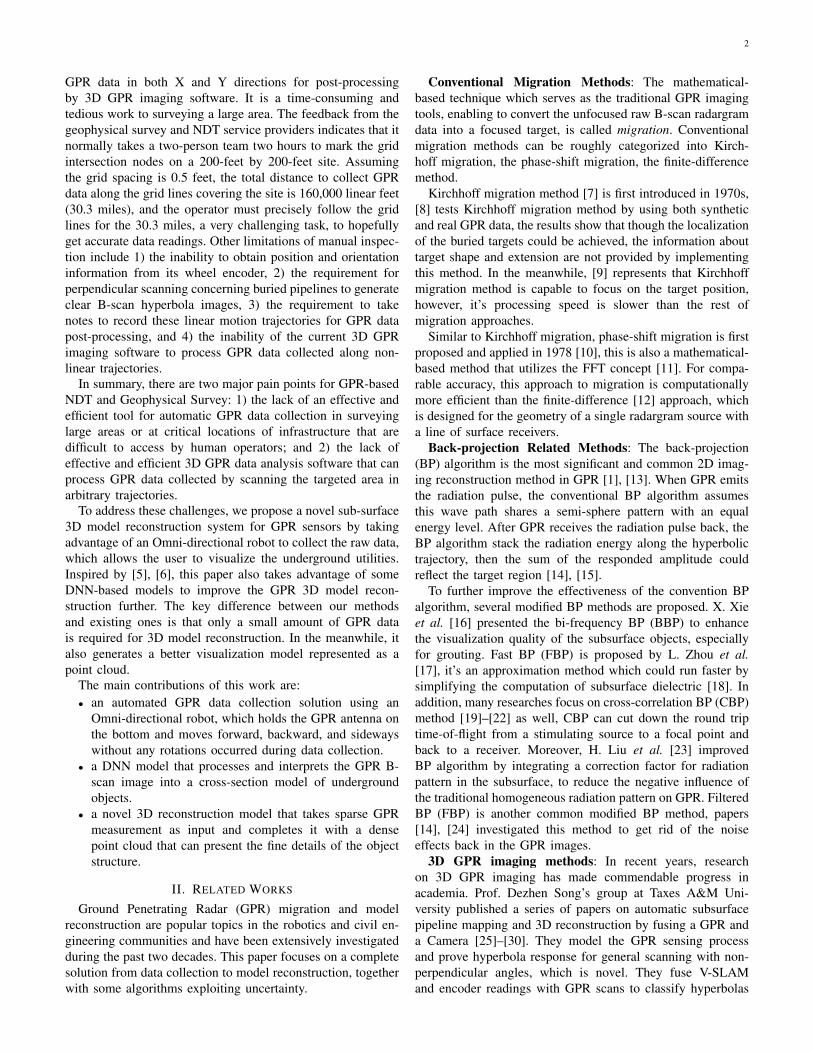
In this section, we introduce an encoder-decoder learningmodel, MigrationNet, to interpret B-scan images. Comparedwith the existing learning-based method of GPR data inter-pretation [37]–[40], our approach does not focus on detectinghyperbola features in the raw B-scan image, because detectionon the GPR B-scan hyperbolic features won’t be helpfulfor GPR data interpretation. MigrationNet takes advantage ofthe back-projection (BP) algorithm. The BP is a process ofaggregation that converts different amplitude of energy into asemi-sphere format at different time. As illustrated in Fig.4,the brighter semi-sphere indicates the higher amplitude partin A-scan. Furthermore, the radius of each semi-sphere in theBP image indicates the depth between the ground and theobject. Hence, MigrationNet emulates the BP principle, stackeach back-projected A-scans into space domain with multi-resolutions, and further interpret them to the cross-sectionimage of the subsurface objects.

Fig. 4. BP algorithm converts the A-scan raw data into a set of semi-spheres.

1) Sparse Back Projection Aggregation: There are somelimitations in the conventional BP approach. First of all, itneeds to back-project each A-scan into a pre-defined 3D

volumetric map, where each A-scan comes from the same B-scan. Second, as each back-projected A-scan is overlapped intoa volumetric map one by one, it leads to heavier computationand processing speed.

To address the above issues, we propose a multi-spatial res-olution input, where the resolution denotes how many A-scanmeasurements from a B-scan are used for back-projection.Specifically, since each B-scan might have a different numberof A-scan measurements, for any B-scan data whose numberof A-scan measurements are less than 1024, we only pick256, 128 and 64 A-scan measurements for back-projectionand stack them in the spatial domain as the input. This ishow we distinguish the different spatial resolution in the inputdata. Otherwise, for those B-scan data with more than 1024A-scan signals, we introduce a sliding-window crop operationover the B-scan raw data to split it into several parts. Thisoperation is equivalent to Equ.2. Note that the length of thesliding window is fixed to 1024 while the width is as same asthe raw B-scan data, which represents the sampling numberof an A-scan measurement.

m = bN/1024c (2)

where N is the number of A-scan measurements in a B-scanand m is the number of cropping B-scans has 1024 A-scansafter the trim operation.

In this way, several M ∗N ∗C 3D stacked input is created,where M demonstrates the number of A-scans in the relatedB-scan, N indicates the number of the sample data in an A-scan measurement, and C is the number of BP data in eachstack group.

We choose to sparsely aggregate the back-projected databecause the proposed MigrationNet can well learn the spatialrelationship from the stacked input data as well as interpretingthe cross-section image of the subsurface cylindrical model.Moreover, this input data with a sparse resolution can decreasethe computational cost and provide richer input informationdue to the multiple resolutions in the spatial domain. Moredetails will be shown in Section III-B and Section V-B2.

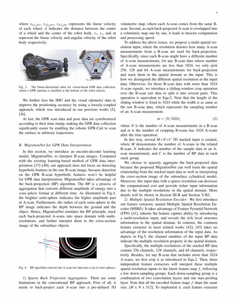
2) Multiple Spatial Resolution Encoder: We first introduceour feature extractor, named Multiple Spatial Resolution En-coder (MSRE). It takes advantage of Feature Pyramid Network(FPN) [41], inherits the feature capture ability by introducinga multi-resolution input, and reveals the rich local structureinformation in the spatial domain. In contrast, the commonfeature extractor in most related works [42], [43] takes noadvantage of the resolution information of the input data. Asdepicts in Fig.5, the channel numbers of the input BP dataindicate the multiple resolution property in the spatial domain.

Specifically, the multiple resolutions of the stacked BP datacontain 256 channels, 128 channels, and 64 channels, respec-tively. Besides, for any B-scan that includes more than 1024A-scans, we first crop it as introduced in Equ.2. Then, threeindependent feature extractors will interpret these multiplespatial resolution inputs to the latent feature map f , followinga few down-sampling groups. Each down-sampling group is acombination of two convolution layers and one max-poolinglayer. Note that all the encoded feature maps f share the samesize: [M x N x 512]. To implement it, each feature extractor

5

Fig. 5. Schematic of the proposed DNN-based migration framework. The input is the stacked BP data with 256 channels and further down-sampling into 128and 64 channels in the spatial domain. Then, the global features are extracted through the multiple spatial resolution encoder and further concatenated into 1536channels. The encoder consists of several de-convolutional groups. The global feature is combined with local features from MSRE through skip-connectionoperation indicated by ⊕ while ¬ to ´ present the last layer feature in each de-convolutional group, and finally decoded into a binary migration image.

has its unique down-sampling group where the kernel sizeof the max-pooling layer is different. In detail, the kernelsize of the max-pooling layer in the 256 channels input is 8.Meanwhile, for 128 channels input, the kernel size of the firstmax-pooling layer is 4, while the rest of the pooling layers’kernel size is equal to 2. As 64 channels sparse input, allthe kernel sizes of max-pooling layers in the down-samplinggroups are 2. As depicts in Fig.5, the different color in theencoder structure indicates the different kernel size of thepooling layer in each down-sampling group.

At last, all three feature maps are then concatenated togetheras F , where size = [M x N x 1536]. This design bringsthe combined latent feature ability to contain better spatialinformation of the input BP data.

3) Decoder: Our decoder consists of 4 up-sampling groups,and each group contains two convolutional layers and onedeconvolutional layer. Besides, we also take advantage ofskip connections as illustrated in Fig.5. The skip-connectionworks on the different encoder layers that have the same size.Specifically, layers ¯ to ± share the same size, and they areconcatenated to the first up-sampling layer. Layer ² and ³ areconcatenated to the second up-sampling layer for the samereason. At last, layer ´ is skip-connected to the third up-sampling layer.

To summarize, the decoder interprets the global feature mapF to a [M x N x 1] migration binary image, where the whiteregion indicates the pipe and the black area indicates thebackground.

4) Loss Design and Training: To constrain the shape andsize of the underground cylindrical object, we develop a jointloss in a two-level hierarchy, pixel, and structure-level, whichcan capture fine structures with clear boundaries. Our hybrid

loss function is composed by following two terms:Firstly, since most of the non-destructive testing objects

have a round shape cross-section (i.e., rebars, utilities, PVCpipes, etc.), we must compare structure similarity between thepredicted image and the ground truth to maintain the propersize and shape. Thus, inspired by [44]–[46], we demonstratethe structure comparison loss between predicted image X andground truth Y as follows:

L1 =σxy +C

σxσy +C(3)

where σx and σy are the standard deviation as an estimate ofthe image contrast, C is a constant value while σxy representsthe covariance which is:

σxy =1

N−1

N

∑i=1

(xi−µx)(yi−µy) (4)

where µx and µy are mean intensity of the predicted imageand ground truth respectively, N is the number of pixels inthe image.

The second loss expression is a common cross entropy lossas proposed in [42]

L2 = ∑xi∈M

w j(x)log(p(xi, j)) (5)

where xi indicates an element in given input while M, p(xi, j)is the element xi probabilistic prediction over class j, and w j

is the weight of each classes.Finally, our loss function could be illustrated as following:

L = λiL1 +λ jL2 (6)

6

Fig. 6. GPRNet framework. The input is a sparse point cloud representing the cross-section of utilities, the encoder abstracts the input as a global feature,and the decoder recovers the global feature to a dense point cloud.

where λi and λ j are the weight of cross entropy loss andstructure loss which satisfy the relation as λi + λ j = 1.

Training: The weights governing the terms in loss functionis set to λi = 0.1 and λ j = 0.9, we also use the stochasticgradient descent (SGD), select momentum as 0.9 and weightdecay as 1e-8. As for the initial learning rate (LR) and inputscale, by evaluating the average accuracy, average precision,average recall as well as F1 score in training dataset withdifferent LR and scale, the learning rate is set to 5e-6 whilethe input scale is 0.25.

IV. GPRNET: GPR PIPES RECONSTRUCTION NETWORKFOR 3D MODELLING

MigrationNet facilitates interpreting the raw B-scan imageinto a cross-section image. However, MigrationNet only pro-vides the 2D slice structure of underground utilities. Even byconcatenating the slices into the 3D space, the obtained 3Dmap is still too sparse to precept. Thus, we manage to completethe gap between this sparse 3D map to recover a dense modelof underground utilities.

Inspired by the 3D point cloud completion works [6], [47]in the computer vision area, we propose GPRNet to obtain adense model of the targets. We firstly represent the interpretedimage, which indicates the cross-section of the undergroundutilities, into the 3D point cloud data format. Our encoder-decoder-based network further completes the sparse input togenerate a fine and dense 3D point cloud reconstruction map.

A. GPRNET Design

1) Encoder: The encoder is an extended version of PCN[6], it represents the geometric information in the input pointcloud with a global feature vector v ∈Rn, n = 896, where thisglobal feature vector is the output of the encoder. Besides, ourencoder implements PointNet layer [48] to extract features,while the PointNet layer is a combination of the convolu-tional multi-layer perceptron (MLP) layer and the max-pooling

layer. This design facilitates our encoder to extract multipleresolution information of the input data, leading to betterperformance on local structure completion.

Specifically, by passing through three MLP layers withdifferent dimensions, our input m×3 point cloud data, wherem is the number of the points set to 1500, is firstly encodedinto three point feature vectors fi, where size is equal to fi :=m× 64, m× 128, m× 256 for i = 1,2,3 respectively. Then,a max-pooling layer is conducted on each extracted featureto obtain three intermediate features g j=1,2,3 with multipledimensions [64− 128− 256]. Furthermore, we concatenateeach point feature vector fi and each intermediate featureg j together to obtain a expanded feature, which includes thefeature information at different level. In addition, each g j isconcatenated to each fi to obtain the feature matrix F, wherethe size is m× 896. At last, F is passed through anotherPointNet layer to generate the global feature vector v.

2) Decoder: The fully-connected decoder [49] is good atpredicting the global geometry of point cloud. However, itignores the local features. While FoldingNet decoder [50]is good at generating a smooth local feature. Taking theadvantages of both decoders, we introduced a decoder as ahierarchical structure similar to [51].

As shown in Fig.6 decoder part, at the top of the decoder,there are three features (size:= 256×3,128×3,64×3) whichare extracted from the global feature by the fully-connectedlayers. Meanwhile, to get a better structure sense of the inputpoint cloud, the global feature is further down-sampled intothe three different levels through the MLP layers. These threedown-sampling features share the size:= 256×3,128×3,64×3as well. Then, the global and local features are concatenatedand represented as an 896× 3 matrix. At last, by takingadvantage of folding operation, a patch of 9 points is generatedat each point in the point set generated from the last step. Thus,we can obtain the detailed output consisting of 896∗9 points.A dense point cloud output is then generated from our multi-resolution decoder, based on the fully-connected and folding

7

operations.Thanks to this multi-resolution architecture, high-level fea-

tures will affect the expression of low-level features. The low-resolution features can contribute to forming the global feature,which provides a sense of the local geometry of the shape.Our experiments show that the prediction of our proposeddecoder has fewer distortions and better-detailed geometry ofthe shape.

3) Loss Design and Training: To constrain and compare thedifference between the output point cloud S and the groundtruth point cloud Sgt , an ideal loss must be differentiableconcerning point locations and invariant to the permutationof the point cloud. In this paper, we use Chamfer Distance(CD) to calculate the average closest point distance betweenS and Sgt , that meets the requirement of the above conditions:

dCD(S,Sgt) =1S ∑

x∈Sminy∈Sgt‖x− y‖2 +

1Sgt

∑y∈Sgt

minx∈S‖y− x‖2 (7)

The Chamfer Distance finds the nearest neighbor in theground truth point set. Thus it can force output point cloudsto lie close to the ground truth and be piecewise smooth.

Training: The training dataset for 3D reconstruction con-tains 306 models while we reserve 18 models for validationand 36 models for testing. The details of dataset setup will beexplained in Section.V-A. Notice that our models are trainedfor 100 epochs with an Adam optimizer. The initial learningrate is set to 0.00005 while the batch size is 16. The weightdecay is 0.7 for every 50000 iterations.

V. EXPERIMENTS STUDY

A. Data Preparation

To verify the proposed DNN models in this paper, we pre-pare a GPR B-scan dataset for training and testing purposes.The dataset we provide contains both synthetic and field B-scan data.

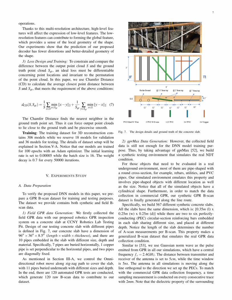
1) Field GPR data Generation: We firstly collected thefield GPR data with our proposed robotics GPR inspectionsystem on a concrete slab at CCNY Robotics Lab TestingPit. Design of our testing concrete slab with different pipesis defined in Fig. 7, our concrete slab have a dimension of96′′× 36′′× 8.5′′ (length×width× thickness), and there are10 pipes embedded in the slab with different size, depth andmaterial. Specifically, 7 pipes are buried horizontally, 1 copperpipe is set perpendicular to the horizontal pipes, and two pipesare diagonally fixed.

As mentioned in Section III-A, we control the Omni-directional robot move along zig-zag path to cover the slab,with 11 pipes buried underneath with different sizes and depth.In the end, there are 120 automated GPR tests are conducted,which generate 120 raw B-scan data to contribute to ourdataset.

Fig. 7. The design details and ground truth of the concrete slab.

2) gprMax Data Generation: However, the collected fielddata is still not enough for the DNN model training pur-pose. Thus, by taking advantage of gprMax [52], we builda synthetic testing environment that simulates the real NDTcondition.

For those objects that need to be evaluated in a realunderground environment, most of them are pipe-shaped witha round cross-section, for example, rebars, utilities, and PVCpipes. Our simulated environment emulates this property andinvolves pipe-shaped objects with different location as wellas the size. Notice that all of the simulated objects have acylindrical shape. Furthermore, in order to match the datacollection in commercial GPR, our synthetic GPR B-scandataset is finally generated along the line route.

Specifically, we build 567 different synthetic concrete slabs.All the slabs have the same dimension, which is: [0.35m (l) x0.25m (w) x 0.25m (d)] while there are two to six perfectly-conducting (PEC) circular-section reinforcing bars embeddedin each slab sharing different size, and placed at differentdepth. Notice the length of the slab determines the numberof A-scan measurements per B-scan. This property makes ageneralized B-scan dataset that emulates the real GPR datacollection condition.

Similar to [53], we use Gaussian norm wave as the pulseemitted from GPR in all our simulations, which have a centralfrequency f c = 2.4GHz. The distance between transmitter andreceiver of the antenna is set to 5cm, while the time windowis 5ns. The antenna in all simulations is moving along theline orthogonal to the direction we set up the PECs. To matchwith the commercial GPR data collection frequency, a timesampling measurement is conducted on every consecutive tracewith 2mm. Note that the dielectric property of the surrounding

8

(a) On-site collected Raw GPR B-scan image (b) Sparse-BP image aggregated in time domain

(c) Predicted migration result with multiple resolution input data (d) Full-BP image aggregated in time domain

(e) Ground-Truth/cross-section image of on-site collected GPR B-scandata

(f) Filtered BP image after applying Hilbert Transform.

Fig. 9. Migration results comparison between our proposed migration method and conventional migration method.

medium in all our slabs is set to 7, which matches with theconcrete dielectric property in the real world. The front viewfigure of our synthetic slabs is shown in Fig.8.

Fig. 8. Some CAD models built by gprMax, which simulate the concreteslab environment where several pipes inserted in.

We conduct 9 times synthetic GPR data collection on eachsimulated slab, with the same spacing between each collection.Therefore, there are 5103 B-scan data are generated in the end.We also generate the point cloud ground truth data accordingto the slab model we created. (The updated GPR dataset willbe released once our work is accepted.)

B. Experiments Study of MigrationNet

1) Effectiveness of MigrationNet: As depicted in Fig.9,Fig.9 (a) shows the collected on-site GPR B-scan data, whichis illustrated in a highlighted hotmap format. Then, Fig.9 (b)and (d) are represented the back-projected data in the timedomain, and are displayed with a highlighted parula colorcode; specifically, figure (b) shows the conventional B-scaninterpretation result with a sparse input BP data, while figure(d) uses the dense BP data as input. In addition, we furtherapply the Hilbert Transform filter in figure (d). The filtered BPimage is shown in figure (f) with a highlighted parula colorcode. At last, figure (e) indicates the ground truth of cross-section image for our collected on-site B-scan data, while

figure (c) demonstrates the B-scan interpretation result fromMigrationNet.

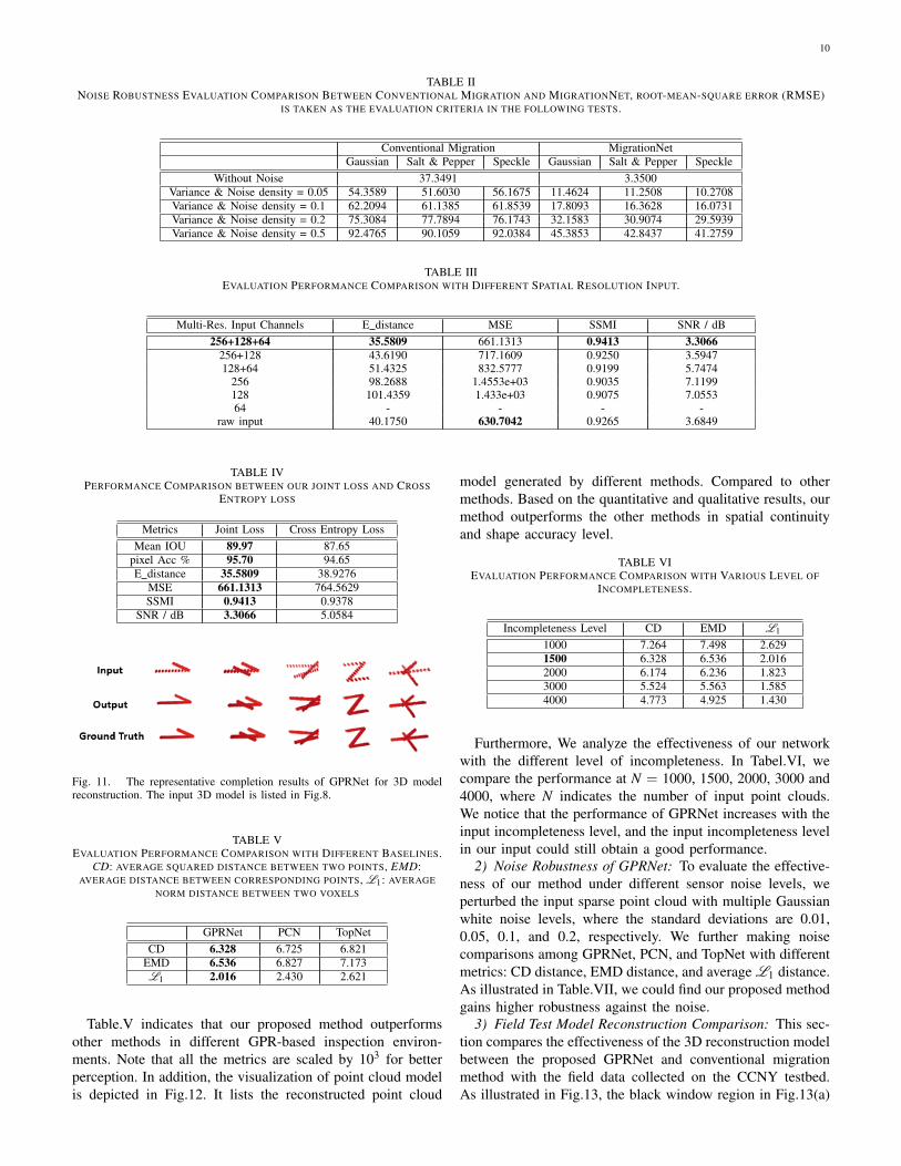
In the meanwhile, quantitative effectiveness comparisonbetween the conventional Migration and MigrationNet aredemonstrated in Table.I. Note that in conventional migrationmethod, the energy level is continuous distributed from 0 to1. In contrast, the energy level in MigrationNet is binarydistributed. That is, 0 stands for the background, and 1presents the target area. Due to this reason, we convert theconventional migration results to the binary image by selectingthe luminance threshold as 0.45. This luminance thresholdwould convert the region where energy level is greater than0.45 to 1, and the rest of the region to 0. In this way, wecan compare the GPR image reconstruction results betweenthe conventional and learning-based methods with multiplemetrics.

The metrics include Mean IOU, Pixel Accuracy, EuclideanDistance (E distance), Mean Square Error (MSE), Signal-to-Noise-Ratio (SNR / dB) and Structural Similarity Index (SSMI).For metrics Mean IOU, Pixel Accuracy, SSMI, the larger thevalue is, the better the performance it stands for; and vice versafor metrics E distance, MSE, SNR. Thus, we can concludethat MigrationNet could effectively improve the performanceof GPR imaging reconstruction.

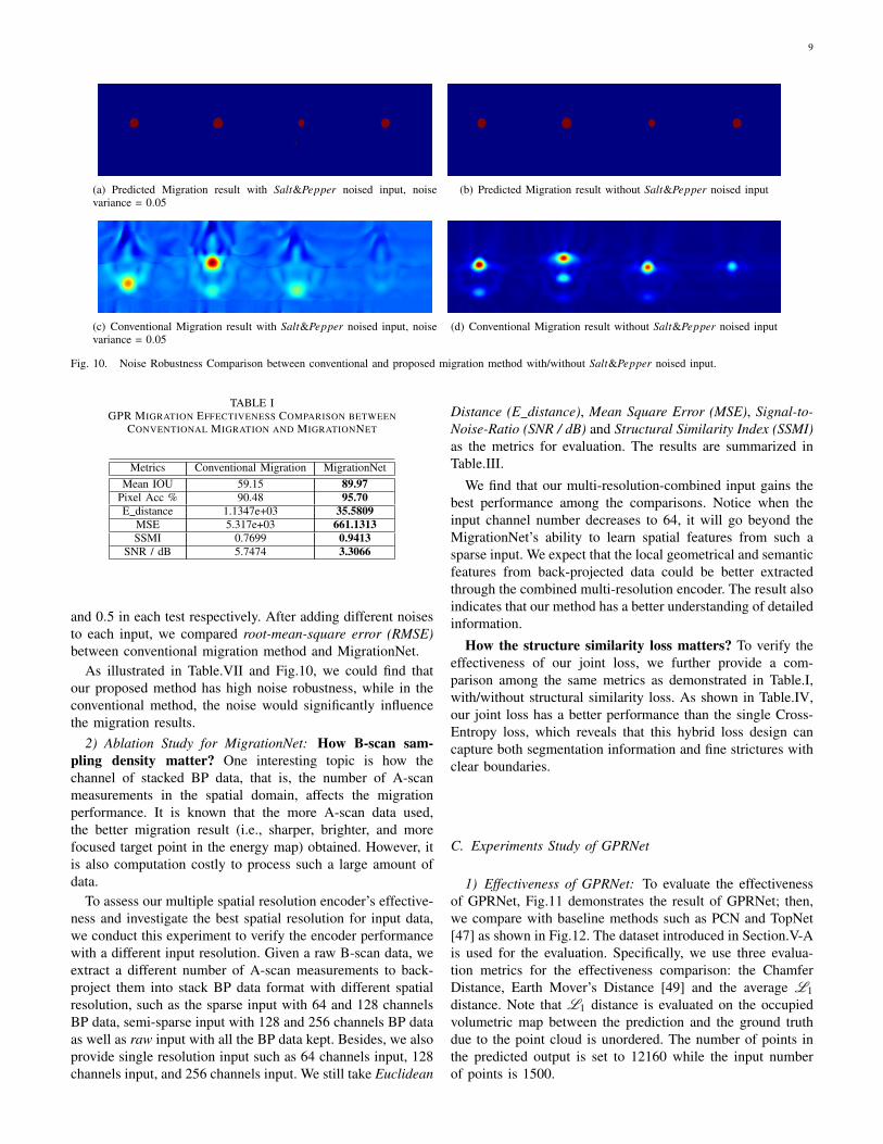
We also test noise robustness in MigrationNet. In thissection, we choose to add Gaussian white noise, salt & peppernoise and speckle noise respectively to the GPR raw data andour stacked BP input data. We conduct 12 sets of experimentson the conventional migration method while another 12 setsof experiments on our proposed method. There are 4 differentvariance and noise density parameters being compared for eachof the noise types. The parameter settings are 0.05, 0.1, 0.2,

9

(a) Predicted Migration result with Salt&Pepper noised input, noisevariance = 0.05

(b) Predicted Migration result without Salt&Pepper noised input

(c) Conventional Migration result with Salt&Pepper noised input, noisevariance = 0.05

(d) Conventional Migration result without Salt&Pepper noised input

Fig. 10. Noise Robustness Comparison between conventional and proposed migration method with/without Salt&Pepper noised input.

TABLE IGPR MIGRATION EFFECTIVENESS COMPARISON BETWEEN

CONVENTIONAL MIGRATION AND MIGRATIONNET

Metrics Conventional Migration MigrationNetMean IOU 59.15 89.97

Pixel Acc % 90.48 95.70E distance 1.1347e+03 35.5809

MSE 5.317e+03 661.1313SSMI 0.7699 0.9413

SNR / dB 5.7474 3.3066

and 0.5 in each test respectively. After adding different noisesto each input, we compared root-mean-square error (RMSE)between conventional migration method and MigrationNet.

As illustrated in Table.VII and Fig.10, we could find thatour proposed method has high noise robustness, while in theconventional method, the noise would significantly influencethe migration results.

2) Ablation Study for MigrationNet: How B-scan sam-pling density matter? One interesting topic is how thechannel of stacked BP data, that is, the number of A-scanmeasurements in the spatial domain, affects the migrationperformance. It is known that the more A-scan data used,the better migration result (i.e., sharper, brighter, and morefocused target point in the energy map) obtained. However, itis also computation costly to process such a large amount ofdata.

To assess our multiple spatial resolution encoder’s effective-ness and investigate the best spatial resolution for input data,we conduct this experiment to verify the encoder performancewith a different input resolution. Given a raw B-scan data, weextract a different number of A-scan measurements to back-project them into stack BP data format with different spatialresolution, such as the sparse input with 64 and 128 channelsBP data, semi-sparse input with 128 and 256 channels BP dataas well as raw input with all the BP data kept. Besides, we alsoprovide single resolution input such as 64 channels input, 128channels input, and 256 channels input. We still take Euclidean

Distance (E distance), Mean Square Error (MSE), Signal-to-Noise-Ratio (SNR / dB) and Structural Similarity Index (SSMI)as the metrics for evaluation. The results are summarized inTable.III.

We find that our multi-resolution-combined input gains thebest performance among the comparisons. Notice when theinput channel number decreases to 64, it will go beyond theMigrationNet’s ability to learn spatial features from such asparse input. We expect that the local geometrical and semanticfeatures from back-projected data could be better extractedthrough the combined multi-resolution encoder. The result alsoindicates that our method has a better understanding of detailedinformation.

How the structure similarity loss matters? To verify theeffectiveness of our joint loss, we further provide a com-parison among the same metrics as demonstrated in Table.I,with/without structural similarity loss. As shown in Table.IV,our joint loss has a better performance than the single Cross-Entropy loss, which reveals that this hybrid loss design cancapture both segmentation information and fine strictures withclear boundaries.

C. Experiments Study of GPRNet

1) Effectiveness of GPRNet: To evaluate the effectivenessof GPRNet, Fig.11 demonstrates the result of GPRNet; then,we compare with baseline methods such as PCN and TopNet[47] as shown in Fig.12. The dataset introduced in Section.V-Ais used for the evaluation. Specifically, we use three evalua-tion metrics for the effectiveness comparison: the ChamferDistance, Earth Mover’s Distance [49] and the average L1distance. Note that L1 distance is evaluated on the occupiedvolumetric map between the prediction and the ground truthdue to the point cloud is unordered. The number of points inthe predicted output is set to 12160 while the input numberof points is 1500.

10

TABLE IINOISE ROBUSTNESS EVALUATION COMPARISON BETWEEN CONVENTIONAL MIGRATION AND MIGRATIONNET, ROOT-MEAN-SQUARE ERROR (RMSE)

IS TAKEN AS THE EVALUATION CRITERIA IN THE FOLLOWING TESTS.

Conventional Migration MigrationNetGaussian Salt & Pepper Speckle Gaussian Salt & Pepper Speckle

Without Noise 37.3491 3.3500Variance & Noise density = 0.05 54.3589 51.6030 56.1675 11.4624 11.2508 10.2708Variance & Noise density = 0.1 62.2094 61.1385 61.8539 17.8093 16.3628 16.0731Variance & Noise density = 0.2 75.3084 77.7894 76.1743 32.1583 30.9074 29.5939Variance & Noise density = 0.5 92.4765 90.1059 92.0384 45.3853 42.8437 41.2759

TABLE IIIEVALUATION PERFORMANCE COMPARISON WITH DIFFERENT SPATIAL RESOLUTION INPUT.

Multi-Res. Input Channels E distance MSE SSMI SNR / dB256+128+64 35.5809 661.1313 0.9413 3.3066

256+128 43.6190 717.1609 0.9250 3.5947128+64 51.4325 832.5777 0.9199 5.7474

256 98.2688 1.4553e+03 0.9035 7.1199128 101.4359 1.433e+03 0.9075 7.055364 - - - -

raw input 40.1750 630.7042 0.9265 3.6849

TABLE IVPERFORMANCE COMPARISON BETWEEN OUR JOINT LOSS AND CROSS

ENTROPY LOSS

Metrics Joint Loss Cross Entropy LossMean IOU 89.97 87.65

pixel Acc % 95.70 94.65E distance 35.5809 38.9276

MSE 661.1313 764.5629SSMI 0.9413 0.9378

SNR / dB 3.3066 5.0584

Fig. 11. The representative completion results of GPRNet for 3D modelreconstruction. The input 3D model is listed in Fig.8.

TABLE VEVALUATION PERFORMANCE COMPARISON WITH DIFFERENT BASELINES.

CD: AVERAGE SQUARED DISTANCE BETWEEN TWO POINTS, EMD:AVERAGE DISTANCE BETWEEN CORRESPONDING POINTS, L1 : AVERAGE

NORM DISTANCE BETWEEN TWO VOXELS

GPRNet PCN TopNetCD 6.328 6.725 6.821

EMD 6.536 6.827 7.173L1 2.016 2.430 2.621

Table.V indicates that our proposed method outperformsother methods in different GPR-based inspection environ-ments. Note that all the metrics are scaled by 103 for betterperception. In addition, the visualization of point cloud modelis depicted in Fig.12. It lists the reconstructed point cloud

model generated by different methods. Compared to othermethods. Based on the quantitative and qualitative results, ourmethod outperforms the other methods in spatial continuityand shape accuracy level.

TABLE VIEVALUATION PERFORMANCE COMPARISON WITH VARIOUS LEVEL OF

INCOMPLETENESS.

Incompleteness Level CD EMD L1

1000 7.264 7.498 2.6291500 6.328 6.536 2.0162000 6.174 6.236 1.8233000 5.524 5.563 1.5854000 4.773 4.925 1.430

Furthermore, We analyze the effectiveness of our networkwith the different level of incompleteness. In Tabel.VI, wecompare the performance at N = 1000, 1500, 2000, 3000 and4000, where N indicates the number of input point clouds.We notice that the performance of GPRNet increases with theinput incompleteness level, and the input incompleteness levelin our input could still obtain a good performance.

2) Noise Robustness of GPRNet: To evaluate the effective-ness of our method under different sensor noise levels, weperturbed the input sparse point cloud with multiple Gaussianwhite noise levels, where the standard deviations are 0.01,0.05, 0.1, and 0.2, respectively. We further making noisecomparisons among GPRNet, PCN, and TopNet with differentmetrics: CD distance, EMD distance, and average L1 distance.As illustrated in Table.VII, we could find our proposed methodgains higher robustness against the noise.

3) Field Test Model Reconstruction Comparison: This sec-tion compares the effectiveness of the 3D reconstruction modelbetween the proposed GPRNet and conventional migrationmethod with the field data collected on the CCNY testbed.As illustrated in Fig.13, the black window region in Fig.13(a)

11

TABLE VIINOISE ROBUSTNESS EVALUATION ON GPRNET WITH THREE METRICS.

GPRNet PCN TopNetCD EMD L1 distance CD EMD L1 distance CD EMD L1 distance

Variance & Noise density = 0.01 6.419 6.628 2.2871 6.901 7.266 2.6187 6.894 7.024 2.5498Variance & Noise density = 0.05 7.722 8.124 2.5648 7.965 8.313 2.7015 8.248 8.480 2.7973Variance & Noise density = 0.1 7.774 8.068 2.6013 8.141 8.458 2.7833 8.489 8.517 2.8571Variance & Noise density = 0.2 8.069 8.369 3.0455 8.495 8.901 2.9559 8.662 8.956 3.1304

Fig. 12. The comparison of completion results between other methods and our network. From left to right: the slab CAD model, input data, PCN [6], TopNet[47], our method and the ground truth. Based on the results, our method could reconstruct a better 3D model for visualization.

(a) Conventional 2D migration result of CCNYtest bed.

(b) 3D model of conventional migration method. (c) Point cloud based 3D model, where the colorindicates the depth of the pipes.

Fig. 13. An illustration of GPR 3D model results. (a) indicates the conventional migration results for our collected field data at the CCNY test bed/concreteslab. (b) shows both the raw and filtered 3D model from the migration result, while (c) shows our proposed 3D reconstruction method, which could reconstructthe 3D point cloud model from the sparse input.

indicates the data collection area while the three 2D imagesdemonstrates migration results from the top view. Note thatthe red pipe in Fig.13(a) could not be recovered, the reasonis that its depth is out of the GPR detection range (See Fig.7

for concrete slab details). Furthermore, we also illustrate rawand filtered 3D model generated by conventional migrationmethods in Fig.13(b). Due to the limitation of the conventionalmigration method, the noise data is hard to be cleaned out

12

and differentiated from the raw GPR data, which causes thefiltered 3D model is still hard to be recognized by normalGPR users. At last, Fig.13(c) illustrates the proposed 3Dmodel reconstruction method, where the color represents thedepth of the pipe. Note that in field test, the positioningaccuracy would affect the distribution of the sparse input,which would introduce the noise in reconstituted point cloudmodel. However, under the supervision of the ground truth,the model could cover the uneven distributed area and fill upwith point clouds, to reveal the real 3D model of the target. Aswe can see, compared with the traditional migration method,our method only requires a sparse input and further generatea fine and continuous output 3D model of underground pipes.It facilitates the GPR users to understand the complex rawGPR B-scan data. In addition to the better performance, usingthe proposed GPR-based robotic inspection platform, the data-collection time is also extremely reduced. Without the roboticdata collection platform, the inspector has to push the GPRdevice along straight lines and move the GPR antenna fromone spot to another, which would take around 5 minutesto scan a 16′′ by 5′ area. However, our robotic-based datacollection only needs less than one minute to automated scanthe same area, which provides a more efficient way for GPRsurvey.

VI. CONCLUSION

This paper presents a novel GPR-based 3D model recon-struction system for underground utilities by using an omni-directional robot. Our omni-directional robot allows the GPRdevice to move forward, backward, and sideways without ro-tations. The proposed system can reconstruct the undergroundutility model represented as a 3D point cloud map. Accordingto the experiments, our approach could obtain a fine 3D modelfor a better visualization while finding out our method hashigher robustness against noise.

ACKNOWLEDGMENT

Financial support for this study was provided by NSF grantIIP-1915721, and by the U.S. Department of Transportation,Office of the Assistant Secretary for Research and Technology(USDOT/OST-R) under Grant No. 69A3551747126 throughINSPIRE University Transportation Center (http://inspire-utc.mst.edu) at Missouri University of Science and Technol-ogy. The views, opinions, findings and conclusions reflectedin this publication are solely those of the authors and do notrepresent the official policy or position of the USDOT/OST-R, or any State or other entity. J Xiao has significant financialinterest in InnovBot LLC, a company involved in R&D andcommercialization of the technology.

REFERENCES

[1] S. Demirci, E. Yigit, I. H. Eskidemir, and C. Ozdemir, “Groundpenetrating radar imaging of water leaks from buried pipes based onback-projection method,” Ndt & E International, vol. 47, pp. 35–42,2012.

[2] GPR-SURVEY, “Gpr-slice,” https://users.neo.registeredsite.com/4/6/6/22358664/assets/GPR-SLICE Software Manual 2021.pdf/, 2021.

[3] leica geosystems, “Leica ds2000 gpr,” https://leica-geosystems.com/en-us/products/detection-systems/utility-detection-solutions/leica-ds2000-utility-detection-radar/, 2021.

[4] usradar, “Quantum mini dual-frequency concrete scanner,” https://usradar.com/quantum-mini-concrete-scanner//, 2021.

[5] J. Feng, L. Yang, H. Wang, Y. Song, and J. Xiao, “Gpr-based subsurfaceobject detection and reconstruction using random motion and depthnet,”in 2020 IEEE International Conference on Robotics and Automation(ICRA). IEEE, 2020, pp. 7035–7041.

[6] W. Yuan, T. Khot, D. Held, C. Mertz, and M. Hebert, “Pcn: Pointcompletion network,” in 2018 International Conference on 3D Vision(3DV). IEEE, 2018, pp. 728–737.

[7] W. A. Schneider, “Integral formulation for migration in two and threedimensions,” Geophysics, vol. 43, no. 1, pp. 49–76, 1978.

[8] X. Liu, M. Serhir, A. Kameni, M. Lambert, and L. Pichon, “Groundpenetrating radar data imaging via kirchhoff migration method,” in2017 International Applied Computational Electromagnetics SocietySymposium-Italy (ACES). IEEE, 2017, pp. 1–2.

[9] N. Smitha, D. U. Bharadwaj, S. Abilash, S. Sridhara, and V. Singh,“Kirchhoff and fk migration to focus ground penetrating radar images,”International Journal of Geo-Engineering, vol. 7, no. 1, p. 4, 2016.

[10] J. Gazdag, “Wave equation migration with the phase-shift method,”Geophysics, vol. 43, no. 7, pp. 1342–1351, 1978.

[11] I. Lecomte, S.-E. Hamran, and L.-J. Gelius, “Improving kirchhoffmigration with repeated local plane-wave imaging? a sar-inspired signal-processing approach in prestack depth imaging,” Geophysical Prospect-ing, vol. 53, no. 6, pp. 767–785, 2005.

[12] J. F. Claerbout and S. M. Doherty, “Downward continuation of moveout-corrected seismograms,” Geophysics, vol. 37, no. 5, pp. 741–768, 1972.

[13] S. Demirci, H. Cetinkaya, E. Yigit, C. Ozdemir, and A. A. Vertiy, “Astudy on millimeter-wave imaging of concealed objects: Application us-ing back-projection algorithm,” Progress In Electromagnetics Research,vol. 128, pp. 457–477, 2012.

[14] R. Schofield, L. King, U. Tayal, I. Castellano, J. Stirrup, F. Pontana,J. Earls, and E. Nicol, “Image reconstruction: Part 1–understandingfiltered back projection, noise and image acquisition,” Journal of car-diovascular computed tomography, vol. 14, no. 3, pp. 219–225, 2020.

[15] M. A. Gonzalez-Huici, I. Catapano, and F. Soldovieri, “A comparativestudy of gpr reconstruction approaches for landmine detection,” IEEEJournal of Selected Topics in Applied Earth Observations and RemoteSensing, vol. 7, no. 12, pp. 4869–4878, 2014.

[16] X. Xie, J. Zhai, and B. Zhou, “Back-fill grouting quality evaluation ofthe shield tunnel using ground penetrating radar with bi-frequency backprojection method,” Automation in Construction, vol. 121, p. 103435.

[17] L. Zhou, C. Huang, and Y. Su, “A fast back-projection algorithm basedon cross correlation for gpr imaging,” IEEE Geoscience and RemoteSensing Letters, vol. 9, no. 2, pp. 228–232, 2011.

[18] A. Gharamohammadi, F. Behnia, and A. Shokouhmand, “Imaging basedon a fast back-projection algorithm considering antenna beamwidth,”in 2019 Sixth Iranian Conference on Radar and Surveillance Systems.IEEE, 2019, pp. 1–4.

[19] J. Cai, P. Peng, H. Zeng, and S. Wang, “A cross correlation based back-projection imaging method for through-wall imaging,” in Journal ofPhysics: Conference Series, vol. 1607, no. 1. IOP Publishing, 2020, p.012020.

[20] C. Lin, X. Wang, Y. Li, F. Zhang, Z. Xu, and Y. Du, “Forward modellingand gpr imaging in leakage detection and grouting evaluation in tunnellining,” KSCE Journal of Civil Engineering, vol. 24, no. 1, pp. 278–294,2020.

[21] S. Jacobsen and Y. Birkelund, “Improved resolution and reduced clut-ter in ultra-wideband microwave imaging using cross-correlated backprojection: Experimental and numerical results,” Journal of BiomedicalImaging, vol. 2010, p. 20, 2010.

[22] H. Zhang, O. Shan, G. Wang, J. Li, S. Wu, and F. Zhang, “Back-projection algorithm based on self-correlation for ground-penetratingradar imaging,” Journal of Applied Remote Sensing, vol. 9, no. 1, p.095059, 2015.

[23] H. Liu, Z. Chen, H. Lu, F. Han, C. Liu, J. Li, and J. Cui, “Migrationof ground penetrating radar with antenna radiation pattern correction,”IEEE Geoscience and Remote Sensing Letters, 2020.

[24] N. Chetih and Z. Messali, “Tomographic image reconstruction usingfiltered back projection (fbp) and algebraic reconstruction technique(art),” in 2015 3rd International Conference on Control, Engineering& Information Technology (CEIT). IEEE, 2015, pp. 1–6.

[25] H. Li, C. Chou, L. Fan, B. Li, D. Wang, and D. Song, “Toward automaticsubsurface pipeline mapping by fusing a ground-penetrating radar and

13

a camera,” IEEE Transactions on Automation Science and Engineering,vol. 17, no. 2, pp. 722–734, 2019.

[26] C. Chou, S.-H. Yeh, J. Yi, and D. Song, “Extrinsic calibration of aground penetrating radar,” in 2016 IEEE International Conference onAutomation Science and Engineering (CASE). IEEE, 2016, pp. 1326–1331.

[27] C. Chou, S.-H. Yeh, and D. Song, “Mirror-assisted calibration of a multi-modal sensing array with a ground penetrating radar and a camera,”in 2017 IEEE/RSJ International Conference on Intelligent Robots andSystems (IROS). IEEE, 2017, pp. 1457–1463.

[28] C. Chou, A. Kingery, D. Wang, H. Li, and D. Song, “Encoder-camera-ground penetrating radar tri-sensor mapping for surface and subsurfacetransportation infrastructure inspection,” in 2018 IEEE InternationalConference on Robotics and Automation (ICRA). IEEE, 2018, pp.1452–1457.

[29] H. Li, C. Chou, L. Fan, B. Li, D. Wang, and D. Song, “Roboticsubsurface pipeline mapping with a ground-penetrating radar and acamera,” in 2018 IEEE/RSJ International Conference on IntelligentRobots and Systems (IROS). IEEE, 2018, pp. 3145–3150.

[30] C. Chou, H. Li, and D. Song, “Encoder-camera-ground penetratingradar sensor fusion: Bimodal calibration and subsurface mapping,” IEEETransactions on Robotics, 2020.

[31] M. Pereira, Y. Zhang, D. Orfeo, D. Burns, D. Huston, and T. Xia, “3dtomography for multistatic gpr subsurface sensing,” in Radar SensorTechnology XXII, vol. 10633. International Society for Optics andPhotonics, 2018, p. 1063302.

[32] M. Pereira, Y. Zhang, D. Huston, and T. Xia, “3-d sar imaging formultistatic gpr,” in Image Sensing Technologies: Materials, Devices,Systems, and Applications VI, vol. 10980. International Society forOptics and Photonics, 2019, p. 109801D.

[33] M. Pereira, Y. Zhang, D. Orfeo, D. Burns, D. Huston, and T. Xia,“3d tomographic image reconstruction for multistatic ground penetratingradar,” in 2019 IEEE Radar Conference (RadarConf). IEEE, 2019, pp.1–6.

[34] M. Pereira, D. Burns, D. Orfeo, Y. Zhang, L. Jiao, D. Huston, and T. Xia,“3-d multistatic ground penetrating radar imaging for augmented realityvisualization,” IEEE Transactions on Geoscience and Remote Sensing,2020.

[35] M. Pereira, D. Burns, D. Orfeo, R. Farrel, D. Hutson, and T. Xia, “Newgpr system integration with augmented reality based positioning,” inProceedings of the 2018 on Great Lakes Symposium on VLSI, 2018, pp.341–346.

[36] L. Yang, G. Yang, Z. Liu, Y. Chang, B. Jiang, Y. Awad, and J. Xiao,“Wall-climbing robot for visual and gpr inspection,” in 2018 13th IEEEConference on Industrial Electronics and Applications (ICIEA). IEEE,2018, pp. 1004–1009.

[37] H. Liu, C. Lin, J. Cui, L. Fan, X. Xie, and B. F. Spencer, “Detectionand localization of rebar in concrete by deep learning using groundpenetrating radar,” Automation in Construction, vol. 118, p. 103279,2020.

[38] J. Gao, D. Yuan, Z. Tong, J. Yang, and D. Yu, “Autonomous pavementdistress detection using ground penetrating radar and region-based deeplearning,” Measurement, p. 108077, 2020.

[39] S. Khudoyarov, N. Kim, and J.-J. Lee, “Three-dimensional convolutionalneural network–based underground object classification using three-dimensional ground penetrating radar data,” Structural Health Moni-toring, p. 1475921720902700, 2020.

[40] U. Ozkaya, F. Melgani, M. B. Bejiga, L. Seyfi, and M. Donelli, “Gprb scan image analysis with deep learning methods,” Measurement, p.107770, 2020.

[41] T.-Y. Lin, P. Dollar, R. Girshick, K. He, B. Hariharan, and S. Belongie,“Feature pyramid networks for object detection,” in Proceedings of theIEEE conference on computer vision and pattern recognition, 2017, pp.2117–2125.

[42] O. Ronneberger, P. Fischer, and T. Brox, “U-net: Convolutional networksfor biomedical image segmentation,” in International Conference onMedical image computing and computer-assisted intervention. Springer,2015, pp. 234–241.

[43] Z. Zhou, M. M. R. Siddiquee, N. Tajbakhsh, and J. Liang, “Unet++:A nested u-net architecture for medical image segmentation,” in DeepLearning in Medical Image Analysis and Multimodal Learning forClinical Decision Support. Springer, 2018, pp. 3–11.

[44] Z. Wang, A. C. Bovik, H. R. Sheikh, and E. P. Simoncelli, “Imagequality assessment: from error visibility to structural similarity,” IEEEtransactions on image processing, vol. 13, no. 4, pp. 600–612, 2004.

[45] H. Zhao, O. Gallo, I. Frosio, and J. Kautz, “Loss functions for neuralnetworks for image processing,” arXiv preprint arXiv:1511.08861, 2015.

[46] C. Godard, O. Mac Aodha, and G. J. Brostow, “Unsupervised monoculardepth estimation with left-right consistency,” in Proceedings of the IEEEConference on Computer Vision and Pattern Recognition, 2017, pp. 270–279.

[47] L. P. Tchapmi, V. Kosaraju, H. Rezatofighi, I. Reid, and S. Savarese,“Topnet: Structural point cloud decoder,” in Proceedings of the IEEEConference on Computer Vision and Pattern Recognition, 2019, pp. 383–392.

[48] C. R. Qi, H. Su, K. Mo, and L. J. Guibas, “Pointnet: Deep learning onpoint sets for 3d classification and segmentation,” in Proceedings of theIEEE conference on computer vision and pattern recognition, 2017, pp.652–660.

[49] P. Achlioptas, O. Diamanti, I. Mitliagkas, and L. Guibas, “Learning rep-resentations and generative models for 3d point clouds,” in Internationalconference on machine learning. PMLR, 2018, pp. 40–49.

[50] Y. Yang, C. Feng, Y. Shen, and D. Tian, “Foldingnet: Point cloudauto-encoder via deep grid deformation,” in Proceedings of the IEEEConference on Computer Vision and Pattern Recognition, 2018, pp. 206–215.

[51] Z. Huang, Y. Yu, J. Xu, F. Ni, and X. Le, “Pf-net: Point fractalnetwork for 3d point cloud completion,” in Proceedings of the IEEE/CVFConference on Computer Vision and Pattern Recognition, 2020, pp.7662–7670.

[52] C. Warren, A. Giannopoulos, and I. Giannakis, “gprmax: Open sourcesoftware to simulate electromagnetic wave propagation for groundpenetrating radar,” Computer Physics Communications, vol. 209, pp.163–170, 2016.

[53] S. Meschino and L. Pajewski, “Spot-gpr: A freeware toolfor targetdetection and localizationin gpr data developedwithin the cost actiontu1208,” Journal of Telecommunications and Information Technology,2017.

Jinglun Feng was born in Jinan, Shandong, China.He received his Master degree in control engineeringfrom the Shandong University in 2015. He is cur-rently pursuing the Ph.D. degree in electrical engi-neering with City College of New York, CUNY, NewYork, NY, USA. His research interests computervision, structural health monitoring, visual SLAMand reconstruction, multi-sensor fusion, and roboticcontrol.

Liang Yang received his B.S. degree from ShenyangAerospace University, Shenyang, China in 2012,and PhD degree in electronics engineering from theCity College of New York (CUNY City College)in 2019, and PhD degree in pattern recognitionand intelligent system from University of ChineseAcademy of Sciences in 2019. He joined APPLEas a senior 3D computer vision researcher in 2019,and currently working on 3D visual perception andunderstanding. His research interests cover motionand path planning, 3D perception and understanding,

visual SLAM and reconstruction, multi-sensor fusion, and robotic control.

Biao Jiang was born in Jiangsu, China. He receiveda Master in Interdisciplinary Studies in 2010, anda PhD in Electrical Engineering in 2013 from theCity College of the City University of New York(CUNY), USA. He currently works at the RoboticsLab of City College of New York as a researchscientist. His research interests include computervision, SLAM and wireless communication.

14

Jizhong Xiao is a Professor of Electrical Engineer-ing at the City College of New York (CCNYCUNYCity College) and a doctoral faculty member ofthe Ph.D. program in Computer Science at CUNYGraduate Center. He received his Ph.D. degree fromMichigan State University in 2002, M.E. degreefrom Nanyang Technological University, Singaporein 1999, M.S, and B.S. degrees from the East ChinaInstitute of Technology, Nanjing, China, in 1993 and1990, respectively. He started the robotics researchprogram at CCNY in 2002 as the founding director

of CCNY Robotics Lab. His current research interests include robotics andcontrol, cyberphysical systems, autonomous navigation and 3D simultaneouslocalization and mapping (SLAM), real-time and embedded computing, as-sistive technology, multiagent systems and swarm robotics. He has publishedmore than 160 research articles in peer reviewed journal and conferences.He received the U.S. National Science Foundation CAREER Award in 2007,the CCNY Outstanding Mentor Award in 2011, and the Humboldt ResearchFellowship for Experienced Researchers from the Alexander von HumboldtFoundation, Germany, from 2013 to 2015. He is a senior member of IEEE.