MAHANAMA-DISSERTATION-2021.pdf - TTU DSpace Principal
106
Risk Assessment and Financial Management of Natural Disasters and Crime by Thilini Vasana Mahanama, M.S. A Dissertation in Mathematics and Statistics Submitted to the Graduate Faculty of Texas Tech University in Partial Fulfillment of the Requirements for the Degree of DOCTOR OF PHILOSOPHY Approved Dr. W. Brent Lindquist Chairperson of the Committee Dr. Dimitri Volchenkov Dr. Svetlozar Rachev Dr. Mark Sheridan Dean of the Graduate School May, 2021
-
Upload
khangminh22 -
Category
Documents
-
view
0 -
download
0
Transcript of MAHANAMA-DISSERTATION-2021.pdf - TTU DSpace Principal

Risk Assessment and Financial Management of Natural Disasters and Crime
by
Thilini Vasana Mahanama, M.S.
A Dissertation
in
Mathematics and Statistics
Submitted to the Graduate Facultyof Texas Tech University in
Partial Fulfillment ofthe Requirements for
the Degree of
DOCTOR OF PHILOSOPHY
Approved
Dr. W. Brent LindquistChairperson of the Committee
Dr. Dimitri Volchenkov
Dr. Svetlozar Rachev
Dr. Mark SheridanDean of the Graduate School
May, 2021

c©2021, Thilini Vasana Mahanama

Texas Tech University, Thilini Mahanama, May 2021
ACKNOWLEDGMENTS
It is with great pleasure that I record my heartfelt indebtedness to my research ad-
visors, Dr. Dimitri Volchenkov, Dr. Svetlozar Rachev, and Dr. W. Brent Lindquist,
for their valuable counsel, guidance, and perseverance throughout my research. Their
continuous encouragement and support have been always a source of inspiration and
energy for me. I am so honored and privileged to have these incredible mentors in
my life.
My heartfelt gratitude also goes out to Dr. D.K. Mallawa Arachchi, my undergrad-
uate research supervisor, at the University of Kelaniya, Sri Lanka. His continuous
advice, guidance, and encouragement immensely helped me to pursue my postgrad-
uate studies at TTU.
I would like to extend my sincere thanks to all the professors in the Department
of Mathematics and Statistics at TTU for helping me in numerous ways during my
graduate studies. I thank the department and graduate school for giving me the
opportunity to pursue my doctoral studies and supporting me with scholarships. I
also wish to thank all my friends at TTU for making these years so memorable.
It is with great appreciation my sincere gratitude is extended to all my professors
at the Department of Mathematics and the Department of Statistics & Computer
Science at the University of Kelaniya, Sri Lanka. I am also grateful to all my teachers
for their valuable guidance and inspiration throughout my education.
I am very much indebted to my colleagues Nadeesha Jayaweera, Mr. Karunarathna
Banda, Dr. Pushpi Paranamana, Abootaleb Shirvani, and Dr. Ann Almeida for their
constant encouragement and support. Valuable experience I received from Toast-
masters International, TTU graduate writing center and library workshops greatly
acknowledged.
I am forever beholden to my parents, sisters, and relatives for their intimacy,
endless patience, and encouragement. They kept me going on and this work would
not have been possible without their input.
ii

Texas Tech University, Thilini Mahanama, May 2021
CONTENTS
ACKNOWLEDGMENTS . . . . . . . . . . . . . . . . . . . . . . . . . . . ii
ABSTRACT . . . . . . . . . . . . . . . . . . . . . . . . . . . . . . . . . . vi
List of Tables . . . . . . . . . . . . . . . . . . . . . . . . . . . . . . . . . . viii
List of Figures . . . . . . . . . . . . . . . . . . . . . . . . . . . . . . . . . . ix
1. Introduction . . . . . . . . . . . . . . . . . . . . . . . . . . . . . . . . . 1
2. Data Description . . . . . . . . . . . . . . . . . . . . . . . . . . . . . . . 5
2.1 Tornado Data Description . . . . . . . . . . . . . . . . . . . . 5
2.2 Crime Data Description . . . . . . . . . . . . . . . . . . . . . . 9
3. Learning a Statistical Manifold to Determine the Risk Covering Strate-
gies for Tornado-induced Property Losses in the United States . . . 14
3.1 Categorizing Tornado Data with respect to Physical Parameters 17
3.2 Exploratory Analysis on Determining Bilateral Coverages for
Tornado Damages . . . . . . . . . . . . . . . . . . . . . . . . . 17
3.3 Assessing a Distance Matrix based on the Differences between
Statistics in Tornado Scales . . . . . . . . . . . . . . . . . . . . 19
3.4 Visualizing the Distances of Property Loss Distributions be-
tween Tornado Scales using Classical Multidimensional Scaling 20
3.5 Learning an Underlying Framework for a Statistical Manifold
on Tornado Property Losses . . . . . . . . . . . . . . . . . . . 21
3.6 Upgrading the Underlying Framework to a Statistical Manifold
using a Subdivision Surface Method . . . . . . . . . . . . . . . 23
3.7 Determining a Curvature Matrix for the Statistical Manifold . 24
3.8 Determining the Risk Assessment Strategy based on the Cur-
vature Matrix . . . . . . . . . . . . . . . . . . . . . . . . . . . 26
4. Assessment of Tornado Property Losses in the United States . . . . . . 29
4.1 Classifying Tornado Data . . . . . . . . . . . . . . . . . . . . . 29
4.1.1 Non-negative Matrix Factorization Method for Classification 29
4.1.2 Classifying Tornado Data Using NMF . . . . . . . . . . . . 31
iii

Texas Tech University, Thilini Mahanama, May 2021
4.2 Measuring the Dependence between Tornado Variables . . . . . 34
4.2.1 Bivariate Copula for Measuring the Non-linear Dependence
between Tornado Variables . . . . . . . . . . . . . . . . . . 34
4.2.2 Measuring the Dependence between Tornado Variables Us-
ing a Bivariate Gaussian Copula Approach . . . . . . . . . 37
4.3 Predicting Tornado Property Losses . . . . . . . . . . . . . . . 40
4.3.1 Long Short-Term Memory Neural Networks for Prediction
of Future Property Losses . . . . . . . . . . . . . . . . . . 40
4.3.2 Predicting Future Tornado-induced Damage Costs Using
LSTM and Shallow Neural Networks . . . . . . . . . . . . 42
5. A Natural Disasters Index . . . . . . . . . . . . . . . . . . . . . . . . . 45
5.1 Construction of the Natural Disasters Index (NDI) . . . . . . . 45
5.2 NDI Option Prices . . . . . . . . . . . . . . . . . . . . . . . . . 48
5.3 NDI Risk Budgets . . . . . . . . . . . . . . . . . . . . . . . . . 53
5.4 Evaluating the Impact of Climate Extreme Indicators on NDI
Performance . . . . . . . . . . . . . . . . . . . . . . . . . . . . 54
6. Global Index on Financial Losses due to Crimes in the United States . . 62
6.1 Financial Losses due to Crimes in the United States . . . . . . 63
6.1.1 Modeling the Multivariate Time Series of Financial Losses
due to Crimes . . . . . . . . . . . . . . . . . . . . . . . . . 63
6.1.2 Backtesting the Portfolio . . . . . . . . . . . . . . . . . . . 63
6.2 Option Prices for the Crime Portfolio . . . . . . . . . . . . . . 66
6.2.1 Defining a Model for Pricing Options . . . . . . . . . . . . 66
6.2.2 Issuing the European Option Prices for the Crime Portfolio 69
6.3 Risk Budgets for the Crime Portfolio . . . . . . . . . . . . . . 70
6.3.1 Defining Tail and Center Risk Measures . . . . . . . . . . . 71
6.3.2 Determining the Risk Budgets for the Crime Portfolio . . . 72
6.4 Performance of the Crime Portfolio for Economic Crisis . . . . 74
6.4.1 Defining Systemic Risk Measures . . . . . . . . . . . . . . 74
6.4.2 Evaluating the Performance of the Crime Portfolio for Eco-
nomic Crisis . . . . . . . . . . . . . . . . . . . . . . . . . . 75
iv

Texas Tech University, Thilini Mahanama, May 2021
7. Discussion & Conclusion . . . . . . . . . . . . . . . . . . . . . . . . . . 77
Bibliography . . . . . . . . . . . . . . . . . . . . . . . . . . . . . . . . . . 80
v
Texas Tech University, Thilini Mahanama, May 2021
ABSTRACT
The National Oceanic and Atmospheric Administration reports that the U.S. an-
nually sustains about 1,300 tornadoes. Currently, the Enhanced Fujita scale is used
to categorize the severity of a tornado event based on a wind speed estimate. We pro-
pose the new Tornado Property Loss scale (TPL-Scale) to classify tornadoes based on
associated damage costs. The dependence between the tornado-affected area and the
associated property losses vary strongly over time and location. The overall tornado
damage costs forecasted by a trained long short-term memory network trained on
historical data might reach $8 billion over the next five years although no systematic
increase in the number and cost of disasters is observed over time.
The approach of compensating for the property losses caused by tornadoes in
the United States is a two-fold process. First, private insurance companies cover the
tornado damage costs claimed by their clients. Second, the state distributes fundings
in the case of state emergency for local governments. We intend to recover these risk
assessment strategies for tornado-induced property losses reported in the national
tornado database. In order to that, we learn a statistical manifold on probability
distributions of property losses and define a measure of curvature on the manifold
to estimate variations of property losses with respect to changes in tornado path
lengths and path widths.
Natural disasters, such as tornadoes, floods, and wildfire pose risks to life and
property, requiring the intervention of insurance corporations. One of the most
visible consequences of changing climate is an increase in the intensity and frequency
of extreme weather events. The relative strengths of these disasters are far beyond
the habitual seasonal maxima, often resulting in subsequent increases in property
losses. Thus, insurance policies should be modified to endure increasingly volatile
catastrophic weather events. We propose a Natural Disasters Index (NDI) for the
property losses caused by natural disasters in the United States based on the “Storm
Data” published by the National Oceanic and Atmospheric Administration. The
proposed NDI is an attempt to construct a financial instrument for hedging the
intrinsic risk. The NDI is intended to forecast the degree of future risk that could
forewarn the insurers and corporations allowing them to transfer insurance risk to
vi

Texas Tech University, Thilini Mahanama, May 2021
capital market investors. This index could also be modified to other regions and
countries.
Following the financial management principles in the NDI, we propose an index-
based insurance portfolio for crime in the United States by utilizing the financial
losses reported by the Federal Bureau of Investigation for property crimes and cy-
bercrimes. Our research intends to help investors envision risk exposure in our port-
folio, gauge investment risk based on their desired risk level, and hedge strategies
for potential losses due to economic crashes. Underlying the index, we hedge the
investments by issuing marketable European call and put options and providing risk
budgets (diversifying risk to each type of crime). We find that real estate, ran-
somware, and government impersonation are the main risk contributors. We then
evaluate the performance of our index to determine its resilience to economic crisis.
The unemployment rate potentially demonstrates a high systemic risk on the portfo-
lio compared to the economic factors used in this study. In conclusion, we provide a
basis for the securitization of insurance risk from certain crimes that could forewarn
investors to transfer their risk to capital market investors.
vii

Texas Tech University, Thilini Mahanama, May 2021
LIST OF TABLES
2.1 The Enhanced Fujita Scale (EF-scale) [1]. . . . . . . . . . . . . . . . 64.1 Kendall’s τ and Spearman’s ρ rank correlation coefficients between
ln(Area) and ln(Loss). . . . . . . . . . . . . . . . . . . . . . . . . . . 395.1 Percent contribution to risk for standard deviation (Std) and expected
tail loss (ETL) (at 95% and 99% levels) risk budgets for the NaturalDisasters Index (NDI) . . . . . . . . . . . . . . . . . . . . . . . . . . 60
5.2 The left-tail systemic risk measures (CoVaR, CoES, and CoETL) onthe Natural Disasters Index (NDI) at different stress levels based onstressing the factors monthly maximum temperature (Max Temp) andthe Palmer Drought Severity Index (PDSI). . . . . . . . . . . . . . . 61
6.1 VaR Backtesting Results for ARMA(1,1)-GARCH(1,1) with Student’st and NIG innovations. . . . . . . . . . . . . . . . . . . . . . . . . . . 65
6.2 The estimated parameters of the fitted the NIG process to the Crimeportfolio log-returns . . . . . . . . . . . . . . . . . . . . . . . . . . . . 67
6.3 The percentages of center risk (CR) and tail risk (TR) (at levels of95% and 99%) budgets for the portfolio on crimes. . . . . . . . . . . . 73
6.4 The empirical correlation coefficients of the joint densities of eacheconomic factors and the crime portfolio . . . . . . . . . . . . . . . . 76
6.5 The left tail systemic risk measures (CoVaR, CoES, and CoETL) onthe portfolio at stress levels of 10%, 5%, and 1% on the following eco-nomic factors - Unemployment Rate, Poverty Rate, Household Income 76
viii

Texas Tech University, Thilini Mahanama, May 2021
LIST OF FIGURES
2.1 According to the NOAA Storm Data reports from 1950-2018, (a) thetotal tornado-induced property losses in states (measured in U.S. dol-lars adjusted for inflation in 2019) and (b) the total numbers of tor-nadoes in Tornado Alley states. Texas has the highest number ofreported tornadoes in Tornado Alley states. . . . . . . . . . . . . . . 6
2.2 The path of a tornado occurred in Raleigh, NC on April 19, 2019,according to National Weather Service, NOAA [2]. . . . . . . . . . . . 6
2.3 In the Tornado Alley states, the annual total numbers of tornadoesdetermined using the NOAA Storm Data reports between 1955 and2018. Over the years, the annual numbers of tornadoes have no com-mon trend. . . . . . . . . . . . . . . . . . . . . . . . . . . . . . . . . . 7
2.4 In the Tornado Alley states, the annual tornado-induced propertylosses (in billions adjusted for inflation in 2019) determined using theNOAA Storm Data reports between 1955 and 2018. Over the years,the annual tornado-induced losses significantly can vary up to billionsof dollars. . . . . . . . . . . . . . . . . . . . . . . . . . . . . . . . . . 8
2.5 Fitted Gaussian distributions for tornado variables: ln(Length), ln(Width),and ln(Loss) (left to right) using the NOAA Storm Data reports be-tween 1955 and 2018. The tornado variables do not hold Gaussiandistributional assumptions. . . . . . . . . . . . . . . . . . . . . . . . . 8
3.1 Kernel density plots for the property losses attributed to tornadoscales in A. Aij represents the tornadoes with path lengths in Liand path widths in Wj. . . . . . . . . . . . . . . . . . . . . . . . . . . 18
3.2 A visual representation of the distance matrix (D) which consists ofthe pairwise Kolmogorov-Smirnov’s distances between the distribu-tions of property losses in tornado scales. . . . . . . . . . . . . . . . . 20
3.3 The underlying framework of the statistical manifold on tornado-induced property losses. Each edge is comprised of the periodic in-terpolating cubic splines and the vertices are the tornado scales inA. The vertex, Aij, represents the tornadoes with lengths in Li andwidths in Wj. . . . . . . . . . . . . . . . . . . . . . . . . . . . . . . . 22
ix

Texas Tech University, Thilini Mahanama, May 2021
3.4 The learned statistical manifold for the property losses of tornadoes,constructed using the reported losses between 1993 and 2018. Aijrepresents the tornadoes with lengths in Li and widths in Wj. Themanifold is constructed by implementing classical dimensional scalingand a method of subdivision surfaces. . . . . . . . . . . . . . . . . . . 23
3.5 (a) The learned statistical manifold and (b) its curvature portrait(right). Figure (b) is constructed with respect to the positions ofthe path width (Wj, j = 1, ..30) and path length (Li, i = 1, ..50)coordinates of a tornado. Yellow and blue regions in Fig (b) depictcompressed and expanded cells in Figure (a), respectively. . . . . . . 25
3.6 The curvature portrait with kernel densities of property losses of somemajor tornado scales in A. The statistics in monochromic zones showsimilar forms. . . . . . . . . . . . . . . . . . . . . . . . . . . . . . . . 27
4.1 The visual representation of the NMF results for tornado data between1950 and 2018. Tornado events and variables are depicted as pointsand vectors, respectively, on the two-dimensional plane constructedby the two salient components of NMF. Tornado events (points) arecolored according to the EF-scale. . . . . . . . . . . . . . . . . . . . . 32
4.2 The visual representation of the NMF results for tornado data duringthe periods 1950-1992 (left) and 1993-2018 (right). Tornado eventsand variables are depicted as points and vectors, respectively, on thetwo-dimensional plane spanned by the two salient components derivedfrom NMF. Tornado events (points) are colored according to the EF-scale. . . . . . . . . . . . . . . . . . . . . . . . . . . . . . . . . . . . . 33
4.3 The histograms of the TPL-Scale (4.5) for the tornado data during (a)1950-1992, (b) 1993-2018, and (c) 1950-2018 are based on the propertylosses reported in NOAA Storm Data. The segment of the TPL-Scalegreater than 60 is magnified in (c); P(TPL−Scale ≥ 60) = 0.025, i.e.,there is a 2.5% chance a tornado will occur causing over ten milliondollars in damages. . . . . . . . . . . . . . . . . . . . . . . . . . . . . 34
4.4 The figures are constructed using the tornado data reported between1955 and 2018 in NOAA Storm Data. Figure (a) provides simplelinear regression analysis: ln(Loss) = 0.59 ln(Area) + 5.06. Figure(b) is the joint density of the generated marginal cdfs of ln(Loss) andln(Area) (F1 and F2, respectively). . . . . . . . . . . . . . . . . . . . 35
x

Texas Tech University, Thilini Mahanama, May 2021
4.5 A sampling distribution of ln(Area): ln(Area) ∼ Γ (18.65, 0.59). Acomparison of the sampled and observed data for ln(Area) (between1955 and 2018 in NOAA Storm Data) using pdf, P-P, and Q-Q plots(left to right). . . . . . . . . . . . . . . . . . . . . . . . . . . . . . . . 38
4.6 A sampling distribution of ln(Loss): ln(Loss) ∼ Γ (15.78, 0.73). Acomparison of the sampled and observed data for ln(Loss) (between1955 and 2018 in NOAA Storm Data) using pdf, P-P, and Q-Q plots(left to right). . . . . . . . . . . . . . . . . . . . . . . . . . . . . . . . 38
4.7 Modeling the joint density of tornado variables, ln(Area) and ln(Loss),using a bivariate Gaussian copula associated with univariate gammadensities (4.11). Applying the generated data, we provide (a) the jointprobability density plot, (b) its contour plot, and (c) a comparison ofthe simulated and the observed data (between 1955 and 2018 in NOAAStorm Data). . . . . . . . . . . . . . . . . . . . . . . . . . . . . . . . 39
4.8 Bivariate Gaussian copula parameters for annual tornado data in Tor-nado Alley states, generated from NOAA Storm Data. There is nomonotonicity in the copula parameters (which provide the correlationof ln(Area) and ln(Loss)) over the years and states. . . . . . . . . . . 40
4.9 The LSTM layer architecture consists of a set of recurrently connectedLSTM blocks. The input, cell state, and output in the tth LSTM blockare denoted as xt, ct, and ht, respectively [4, 5]. . . . . . . . . . . . . 41
4.10 The structure of the tth LSTM block: The multiplicative units areinput (i), forget (f), and output (o) gates, and the cell state (g). Theinput, cell state, and output in the tth memory cell are denoted asxt, ct, and ht, respectively [4, 5]. . . . . . . . . . . . . . . . . . . . . . 42
4.11 A comparison of the observed and simulated monthly losses caused bytornadoes between 1990 and 2018 (testing data) and the errors due topredictions using a LSTM network. The simulations were generatedusing NOAA Storm Data. . . . . . . . . . . . . . . . . . . . . . . . . 43
4.12 The predictions of the monthly tornado-induced property losses in2019 (in millions) (a) using a LSTM and (b) using a shallow neu-ral network. The box plots in (b) are constructed using the 10,000simulations generated for each month based on NOAA Storm Data. . 44
xi

Texas Tech University, Thilini Mahanama, May 2021
4.13 The predictions of (a) the monthly tornado-induced property lossesand (b) the cumulative monthly property losses (in billions adjustedfor inflation in 2019) between 2020 and 2025 using a LSTM network.The higher losses would be reported from March to June, and thevolume of property losses would amount up to eight billion dollars in2025. The simulations were generated using NOAA Storm Data. . . . 44
5.1 The monthly property losses (in billions adjusted for inflation in 2019)caused by drought, flood, winter storm, thunderstorm wind, hail, andtornado events between 1996 and 2018 generated using NOAA StormData. . . . . . . . . . . . . . . . . . . . . . . . . . . . . . . . . . . . . 46
5.2 Our proposed Natural Disasters Index (NDI) for the United States.This NDI (5.1) is constructed using the property losses of naturaldisasters reported in NOAA Storm Data between 1996 and 2018. . . . 47
5.3 The first differences of the stress testing variables, (a) Maximum Tem-perature (Max Temp) and (b) Palmer Drought Severity Index (PDSI),yield stationary time series. . . . . . . . . . . . . . . . . . . . . . . . 48
5.4 The call option prices (5.7) for the Natural Disasters Index (NDI) attime t for a given strike price K using a GARCH(1,1) model withgeneralized hyperbolic innovations. . . . . . . . . . . . . . . . . . . . 51
5.5 The put option prices (5.8) for the Natural Disasters Index (NDI) attime t for a given strike price K using a GARCH(1,1) model withgeneralized hyperbolic innovations. . . . . . . . . . . . . . . . . . . . 52
5.6 The call and put option prices for the Natural Disasters Index (NDI)at time t for a given strike price K using a GARCH(1,1) model withgeneralized hyperbolic innovations. . . . . . . . . . . . . . . . . . . . 52
5.7 The Natural Disasters Index (NDI) implied volatilities against timeto maturity (T ) and moneyness (M = S/K, where S and K thestock and strike prices, respectively) using a GARCH(1,1) model withgeneralized hyperbolic innovations. . . . . . . . . . . . . . . . . . . . 53
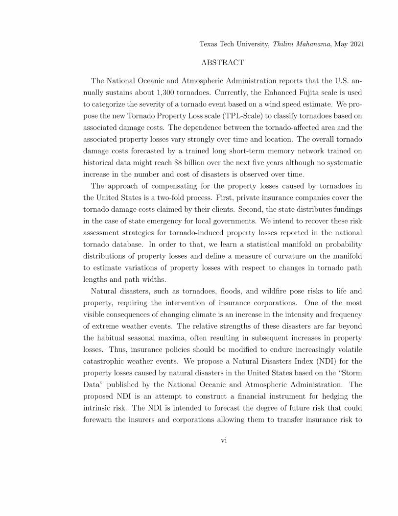
5.8 The percent contribution to risk (PCTR) of the expected tail loss(ETL) risk budgets for the Natural Disasters Index (NDI) at 95%level. The legend depicts the severe weather events in ascending orderof their PCTR of ETL risk budgets at 95% level. . . . . . . . . . . . 55
5.9 The percent contribution to risk (PCTR) of the expected tail loss(ETL) risk budgets for the Natural Disasters Index (NDI) at 99%level. The legend depicts the severe weather events in ascending orderof their PCTR of ETL risk budgets at 99% level. . . . . . . . . . . . 56
xii

Texas Tech University, Thilini Mahanama, May 2021
5.10 The percent contribution to risk (PCTR) of the standard deviation(Std) risk budgets for the Natural Disasters Index (NDI). The legenddepicts the severe weather events in ascending order of their PCTR ofStd risk budgets. . . . . . . . . . . . . . . . . . . . . . . . . . . . . . 57
5.11 The generated joint densities of the returns of monthly maximum tem-perature (Max Temp) and the Natural Disasters Index (NDI), andthe Palmer Drought Severity Index (PDSI) and the NDI (right panel)using the fitted bivariate NIG models of the joint distributions ofindependent and identically distributed standardized residuals. Thefigures depict the simulated values and the contour plots of the jointdensities. . . . . . . . . . . . . . . . . . . . . . . . . . . . . . . . . . . 58
6.1 Call option prices against time to maturity (T , in days) and strikeprice (K, based on S0 = 100). . . . . . . . . . . . . . . . . . . . . . . 69
6.2 Put option prices against time to maturity (T , in days) and strikeprice (K, based on S0 = 100). . . . . . . . . . . . . . . . . . . . . . . 70
6.3 Implied volatility surface against time to maturity (T , in days) andmoneyness (M = K/S, the ratio of strike price, K, and stock price, S). 71
xiii

Texas Tech University, Thilini Mahanama, May 2021
CHAPTER 1
INTRODUCTION
The National Centers for Environmental Information reports the United States
has experienced 69 natural disasters with losses exceeding one billion dollars between
2015 and 2019. The accumulated loss exceeds $535 billion at an average of $107.1
billion/year. The trend of disaster frequency is expected to escalate over the years
due to changes in climate which will result in catastrophic losses [6]. These volatile
weather patterns will result in an inevitable challenge to the U.S.’s ability to sustain
human and economic development [7]. As a result, weather risk markets need to be
capable of offsetting the financial impacts of natural disasters [8, 9].
The financial losses due to natural disasters exacerbate due to changes in popula-
tion and national wealth density [10, 11]. If insurers are to retain profitability and
solvency in the event of a major catastrophe that insurers must increase their prices
for catastrophe insurance and reduce their exposure to risk [12]. Also, reinsurers un-
dergo severe financial stress in facilitating catastrophe insurance by offering tenable
reduction for risk in large catastrophic losses [13, 14, 15]. However, the substantial
losses can be alleviated using protective measures such as preparedness, mitigation,
and insurance [16, 17]. To better protect the clients, catastrophe insurance policies
should ramp-up investments in cost-effective loss reduction mechanisms by better
managing the risk.
Unequivocally, the catastrophe losses and related risks inherent create uncertainty
over the type of disaster event [13, 18]. For example, due to less coverage of insured
assets and data latency in drought and flooding events, they tend to provide uncertain
loss estimates compared to the losses of severe storm events in the United States
[18, 19]. In consequence, prioritization for mitigating the risks can be diverse and
complex.
In this dissertation, we address the risk assessment strategies for tornadoes re-
ported in NOAA Storm Data [3] in chapter 3 and 4. We consider the reported finan-
cial losses for tornadoes without considering their temporal relationships. Then, we
discuss the risk assessment strategies from the perspective of the compensations for
1

Texas Tech University, Thilini Mahanama, May 2021
tornado property damages.
In the United States, the approach of compensating the property losses caused by
tornadoes is a two-pronged strategy. First, private insurance companies cover the
tornado damage costs claimed by their clients. Second, the state distributes fundings
in the case of state emergency for local governments. We intend to recover the risk
assessment strategies for tornado-induced property losses reported in the database
[3]. Therefore, we learn a statistical manifold on probability distributions of property
losses to describe the processes of risk evaluations.
We categorize tornado data with respect to tornado path lengths and tornado path
widths and determine their probability distributions of property losses in sections
3.1 and 3.2. Then, we construct a distance matrix using the pairwise Kolmogorov-
Smirnov’s distances [20] in terms of property losses between tornado categories in
section 3.3. Henceforth, we learn a statistical manifold using classical multidimen-
sional scaling [21] for the distance matrix and a subdivision surface method in sec-
tions 3.4 - 3.6. Then, we define a measure of curvature on the statistical manifold to
show the existence of different risk assessment strategies for tornado-induced prop-
erty losses in sections 3.7 and 3.8. Finally, we generalize this procedure to introduce
the “Statistical Manifold Learning Algorithm” for high dimensional data.
In chapter 4, we address three problems in assessing tornado-induced property
losses. First, we introduce a new scale (known as TPL-Scale) in addition to the
Enhanced Fujita Scale [1] to classify tornadoes based on their financial impacts due
to damages using the non-negative matrix factorization analysis [22] in section 4.1.
Second, we apply a copula approach [23] for assessing property losses based on its
dependence on the area affected by tornadoes in section 4.2. Third, we predict
future tornado damage costs in section 4.3 using the shallow and the long short-term
memory neural networks. Based on our findings, the volume of tornado-induced
property losses would amount up to eight billion dollars by 2025.
The risk assessment strategies outline in chapter 3 and 4 cannot be implemented
for natural disasters other than tornadoes due to the lack of reported data in [3].
For that reason, we integrate the reported property losses in all types of natural
disasters taking the temporal ordering into account. Then, we utilize the time series
2

Texas Tech University, Thilini Mahanama, May 2021
of financial losses for hedging the risk due to natural disasters in chapter 5.
The weather index insurance can effectively transfer spatially covariate weather
risks as it pays indemnities based on realizations of a weather index that is highly
correlated with actual losses [24]. The securitization of losses from natural disas-
ters provides a valuable novel source of diversification for investors. Catastrophe
risk bonds are a promising type of insurance-linked securities introduced to smooth
transferring of catastrophic insurance risk from insurers and corporations to capital
market investors by offering an alternative or complement of capital to the traditional
reinsurance [15]. The three types of variables that pay off in insurance-linked secu-
rities [25] are insurer-specific catastrophe losses, insurance-industry catastrophe loss
indices, and parametric indices based on the physical characteristics of catastrophic
events.
The first index-based catastrophe derivatives, CAT-futures, introduced by the
Chicago Board of Trade using the ISO-Index was ineffective due to a lack of re-
alistic models in the market [26]. Secondly, the Property Claim Services (PCS)
proposed the PCS-options based on the PCS-index and they slowed down due to
market illiquidity [27]. Then, the New York Mercantile Exchange (NYMEX) de-
signed catastrophe futures and options to enhance the transparency and liquidity
of the capital markets to the insurance sector [27]. [28] further explains alternative
risk transfer mechanisms within the context of natural catastrophe problems in the
United States.
We propose Natural Disasters Index (NDI) to address these shortcomings by cre-
ating a financial instrument for hedging the intrinsic risk induced by the property
losses caused by natural disasters in the U.S. The vital objective of the NDI is to
forecast the severity of future systemic risk attributed to natural disasters. This pro-
vides advance warnings to the insurers and corporations allowing them to transfer
insurance risk to capital market investors. Therefore, the proposed NDI is intended
to make up the shortfall between the capital and insurance markets. The NDI identi-
fies the potential risk contributions of each natural disaster and provides options and
futures in sections 5.2 and 5.3. In addition, we assess the performance of the NDI to
adverse weather events in section 5.4. Furthermore, the NDI could be modified to
3

Texas Tech University, Thilini Mahanama, May 2021
calculate the risk in other regions or countries using a data set comparable to NOAA
Storm Data [3].
We follow the methods applied in the NDI on an ad hoc basis as a benchmark
to investigate the financial impact of crimes in the U.S. Using the financial losses
due to various types of crimes reported by the Federal Bureau of Investigation, we
propose a portfolio based on the economic impacts of these crimes in chapter 6. The
objective of this portfolio is to examine the impact of crime on insurance policies in
the United States by analyzing the financial losses associated with property crimes
and cybercrimes. Therefore, the key findings are intended to provide a basis for
the securitization of insurance risk from crimes. We investigate the financial market
implications of the portfolio using option pricing theory as well as risk budgeting
in sections 6.1 - 6.3. Furthermore, we evaluate the performance of our index with
respect to economic factors using stress testing in section 6.4.
4

Texas Tech University, Thilini Mahanama, May 2021
CHAPTER 2
DATA DESCRIPTION
2.1 Tornado Data Description
National Oceanic and Atmospheric Administration (NOAA)’s National Centers for
Environmental Information reports severe weather events that have great impacts on
the U.S. economy. The total cost of the climate disasters since 1980 exceeds $1.775
trillion [18]. The U.S. sustains about 1,300 tornadoes and loses around fifty people
annually [3, 29]. In Figure 2.1(a), we have shown tornado property losses reported in
the U.S. in US dollars adjusted for 2019. Texas, Oklahoma, Kansas, Iowa, Missouri,
and Nebraska form a region with a disproportionately high frequency of tornadoes
known as Tornado Alley. Tornadoes in this region typically happen in late spring
and occasionally the early fall [30]. Texas alone experienced around 4,000 tornado
events since records began in 1950 [3], see Figure 2.1(b). These disastrous events
resulted in many deaths and had significant economic effects on the areas impacted.
In the United States, over 69,000 tornadoes have been reported by NOAA [3]
during the period from 1950 to 2018. For the recorded tornado events, the database
reports path length and width (measured in miles and feet, respectively) and property
losses (measured in U.S. Dollars of the given year). For example, Figure 2.2 illustrates
a path of a tornado in Raleigh, NC on April 19, 2019. Whenever appropriate, we
approximate the area affected by a tornado as the product of path length and width
(measured in square feet). We estimate property losses in U.S. dollars of 2019.
Tornado intensity, assessed by the Enhanced Fujita Scale (EF-scale) [1], assigns
each tornado a ‘rating’ based on estimated wind speed and related possible damages.
For each tornado in [3], the tornado intensity is characterized by one of six scales
[31] with an increasing degree of damage given by the EF-scale, see Table 2.1.
5

Texas Tech University, Thilini Mahanama, May 2021
0
2,000,000,000
4,000,000,000
6,000,000,000
Total Losses (USD 2019) 1950 − 2018
(a) (b)
Figure 2.1: According to the NOAA Storm Data reports from 1950-2018, (a) thetotal tornado-induced property losses in states (measured in U.S. dollars adjustedfor inflation in 2019) and (b) the total numbers of tornadoes in Tornado Alley states.Texas has the highest number of reported tornadoes in Tornado Alley states.
Figure 2.2: The path of a tornado occurred in Raleigh, NC on April 19, 2019,according to National Weather Service, NOAA [2].
Table 2.1: The Enhanced Fujita Scale (EF-scale) [1].
EF-scale Wind Speed Estimate (mph) Damage Description
EFO 65–85 Minor
EF1 86–110 Moderate
EF2 111–135 Considerable
EF3 136–165 Severe
EF4 166–200 Devastating
EF5 ≥ 200 Incredible
6

Texas Tech University, Thilini Mahanama, May 2021
NOAA has identified Florida and the South-Central U.S. as having a dispropor-
tionately high frequency of tornadoes [3], see Figure 2.1. Texas, Oklahoma, Kansas,
Nebraska, Iowa, and Missouri are widely known as Tornado Alley [30]. They display
high fluctuations in the annual numbers of tornadoes that occurred between 1955 and
2018, see Figure 2.3. The quadratic trendline fits (curves in red) exemplify that the
trends are not monotonic over the years. Furthermore, the annual tornado-induced
property losses in the Tornado Alley states vary up to nine orders of magnitude (i.e.
billions of dollars), see Figure 2.4.
1960 1980 2000Year
0
50
100
150
200
250
No
of T
orna
does
Texas
1960 1980 2000Year
0
20
40
60
80
100
No
of T
orna
does
Oklahoma
1960 1980 2000Year
0
20
40
60
80
No
of T
orna
does
Kansas
1960 1980 2000Year
0
20
40
60
80
No
of T
orna
does
Iowa
1960 1980 2000Year
0
20
40
60
80
100
No
of T
orna
does
Missouri
1960 1980 2000Year
0
20
40
60
80
No
of T
orna
does
Nebraska
Figure 2.3: In the Tornado Alley states, the annual total numbers of tornadoesdetermined using the NOAA Storm Data reports between 1955 and 2018. Over theyears, the annual numbers of tornadoes have no common trend.
We fit Gaussian distributions for tornado variables (i.e., path length, path width,
and property loss), see Figure 2.5. The assumptions of normality do not hold for
tornado variables as depicted in Figure 2.5 [32]. We use a copula approach for the
bivariate non-Gaussian distributed tornado affected areas and property losses [33, 34].
We thus investigate the dependence between tornado-affected areas and attributed
property losses in section 4.2.2.
7

Texas Tech University, Thilini Mahanama, May 2021
1960 1980 2000Year
0
1
2
3
Loss
(bi
llion
s $
2019
)
Texas
1960 1980 2000Year
0
0.5
1
1.5
2
2.5
Loss
(bi
llion
s $
2019
)
Oklahoma
1960 1980 2000Year
0
0.5
1
1.5
2
2.5
Loss
(bi
llion
s $
2019
)
Kansas
1960 1980 2000Year
0
0.5
1
1.5Lo
ss (
billi
ons
$ 20
19)
Iowa
1960 1980 2000Year
0
1
2
3
4
Loss
(bi
llion
s $
2019
)
Missouri
1960 1980 2000Year
0
0.5
1
1.5
Loss
(bi
llion
s $
2019
)
Nebraska
Figure 2.4: In the Tornado Alley states, the annual tornado-induced property losses(in billions adjusted for inflation in 2019) determined using the NOAA Storm Datareports between 1955 and 2018. Over the years, the annual tornado-induced lossessignificantly can vary up to billions of dollars.
Figure 2.5: Fitted Gaussian distributions for tornado variables: ln(Length),ln(Width), and ln(Loss) (left to right) using the NOAA Storm Data reports be-tween 1955 and 2018. The tornado variables do not hold Gaussian distributionalassumptions.
8

Texas Tech University, Thilini Mahanama, May 2021
2.2 Crime Data Description
In this section, we define the types of crimes utilized for constructing our index.
Using official data published by the Federal Bureau of Investigation (FBI), we con-
sidered financial losses caused by crimes committed in the United States between
2001 and 2019. We use the FBI’s Internet Crime Reports [35] to estimate the fi-
nancial losses attributed to cybercrimes and Uniform Crime Reports [36] to assess
the financial losses caused by property crimes (burglary, larceny-theft, and motor
vehicle theft). Using the information collected from these two reports, we calculate
the cumulative financial losses reported for the following 32 types of crimes [35, 37]:
• Advanced Fee: An individual pays money to someone in anticipation of
receiving something of greater value in return, but instead receives significantly
less than expected or nothing.
• BEA/EAC (Business Email Compromise/Email Account Compro-
mise): BEC is a scam targeting businesses working with foreign suppliers
and/or businesses regularly performing wire transfer payments. EAC is a sim-
ilar scam that targets individuals. These sophisticated scams are carried out
by fraudsters compromising email accounts through social engineering or com-
puter intrusion techniques to conduct unauthorized transfer of funds.
• Burglary: The unlawful entry of a structure to commit a felony or a theft.
Attempted forcible entry is included.
• Charity: Perpetrators set up false charities, usually following natural disas-
ters, and profit from individuals who believe they are making donations to
legitimate charitable organizations.
• Check Fraud: A category of criminal acts that involve making the unlawful
use of cheques in order to illegally acquire or borrow funds that do not exist
within the account balance or account-holder’s legal ownership.
• Civil Matter: Civil lawsuits are any disputes formally submitted to a court
that is not criminal.
9

Texas Tech University, Thilini Mahanama, May 2021
• Confidence Fraud/Romance: A perpetrator deceives a victim into believ-
ing the perpetrator and the victim have a trust relationship, whether family,
friendly or romantic. As a result of that belief, the victim is persuaded to send
money, personal and financial information, or items of value to the perpetra-
tor or to launder money on behalf of the perpetrator. Some variations of this
scheme are romance/dating scams or the grandparent scam.
• Corporate Data Breach: A leak or spill of business data that is released
from a secure location to an untrusted environment. It may also refer to a
data breach within a corporation or business where sensitive, protected, or
confidential data is copied, transmitted, viewed, stolen, or used by an individual
unauthorized to do so.
• Credit Card Fraud: Credit card fraud is a wide-ranging term for fraud com-
mitted using a credit card or any similar payment mechanism as a fraudulent
source of funds in a transaction.
• Crimes Against Children: Anything related to the exploitation of children,
including child abuse.
• Denial of Service: A Denial of Service (DoS) attack floods a network/system
or a Telephony Denial of Service (TDoS) floods a service with multiple requests,
slowing down or interrupting service.
• Employment: Individuals believe they are legitimately employed, and lose
money or launders money/items during the course of their employment.
• Extortion: Unlawful extraction of money or property through intimidation or
undue exercise of authority. It may include threats of physical harm, criminal
prosecution, or public exposure.
• Gambling: Online gambling, also known as Internet gambling and iGambling,
is a general term for gambling using the Internet.
10

Texas Tech University, Thilini Mahanama, May 2021
• Government Impersonation: A government official is impersonated in an
attempt to collect money.
• Harassment/Threats of Violence: Harassment occurs when a perpetrator
uses false accusations or statements of fact to intimidate a victim. Threats
of Violence refers to an expression of an intention to inflict pain, injury, or
punishment, which does not refer to the requirement of payment.
• Identity Theft: Identify theft involves a perpetrator stealing another per-
son’s personal identifying information, such as name or Social Security number,
without permission to commit fraud.
• Investment: A deceptive practice that induces investors to make purchases
on the basis of false information. These scams usually offer the victims large
returns with minimal risk. Variations of this scam include retirement schemes,
Ponzi schemes, and pyramid schemes.
• IPR Copyright: The theft and illegal use of others’ ideas, inventions, and
creative expressions, to include everything from trade secrets and proprietary
products to parts, movies, music, and software.
• Larceny Theft: The unlawful taking, carrying, leading, or riding away of
property (except motor vehicle theft) from the possession or constructive pos-
session of another.
• Lottery/Sweepstakes: Individuals are contacted about winning a lottery
or sweepstakes they never entered, or to collect on an inheritance from an
unknown relative and are asked to pay a tax or fee in order to receive their
award.
• Misrepresentation: Merchandise or services were purchased or contracted
by individuals online for which the purchasers provided payment. The goods
or services received were of measurably lesser quality or quantity than was
described by the seller.
11

Texas Tech University, Thilini Mahanama, May 2021
• Motor Vehicle Theft: The theft or attempted theft of a motor vehicle.
A motor vehicle is self-propelled and runs on land surface and not on rails.
Motorboats, construction equipment, airplanes, and farming equipment are
specifically excluded from this category.
• Non-Payment/Non-Delivery: In non-payment situations, goods and ser-
vices are shipped, but payment is never rendered. In non-delivery situations,
payment is sent, but goods and services are never received.
• Overpayment: An individual is sent a payment/commission and is instructed
to keep a portion of the payment and send the remainder to another individual
or business.
• Personal Data Breach: A leak or spill of personal data that is released from
a secure location to an untrusted environment. It may also refer to a security
incident in which an individual’s sensitive, protected, or confidential data is
copied, transmitted, viewed, stolen, or used by an unauthorized individual.
• Phishing/Vishing/Smishing/Pharming: Unsolicited email, text messages,
and telephone calls purportedly from a legitimate company requesting personal,
financial, and/or login credentials.
• Ransomware: A type of malicious software designed to block access to a
computer system until money is paid.
• Real Estate/Rental: Fraud involving real estate, rental, or timeshare prop-
erty.
• Robbery: The taking or attempting to take anything of value from the care,
custody, or control of a person or persons by force or threat of force or violence
and/or by putting the victim in fear.
• Social Media: A complaint alleging the use of social networking or social
media (Facebook, Twitter, Instagram, chat rooms, etc.) as a vector for fraud.
Social Media does not include dating sites.
12

Texas Tech University, Thilini Mahanama, May 2021
• Terrorism: Violent acts intended to create fear that are perpetrated for a
religious, political, or ideological goal and deliberately target or disregard the
safety of non-combatants.
Whenever necessary, we use multiple imputations with the principal component
analysis model to compute missing data [38]. Moreover, we adjust the financial
losses for U.S. dollars in 2020 using the CPI Inflation Calculator available in the
U.S. Bureau of Labor Statistics. Then, we model the time series of financial losses
due to these crime types in section 6.1.1.
13

Texas Tech University, Thilini Mahanama, May 2021
CHAPTER 3
LEARNING A STATISTICAL MANIFOLD TO DETERMINE THE RISK
COVERING STRATEGIES FOR TORNADO-INDUCED PROPERTY LOSSES
IN THE UNITED STATES
In the United States, the approach of compensating the property losses caused by
tornadoes is a two-pronged strategy. First, private insurance companies cover the
tornado damage costs claimed by their clients. Second, the state distributes fundings
in the case of state emergency for local governments. We intend to recover the risk
assessment strategies for tornado-induced property losses reported in the database
[3]. In order to accomplish this, we learn a statistical manifold on probability distri-
butions of property losses to describe the processes of risk evaluations.
We develop a “Statistical Manifold Learning Algorithm” to learn a statistical man-
ifold for tornado property losses reported between 1993 and 2019 [3] . First, we cat-
egorize tornado data with respect to the physical parameters (tornado path lengths
and tornado path widths) in section 3.1. In section 3.2, we determine the probability
distributions of property losses in each tornado scale. Then, we assess pairwise differ-
ences of distributions of property losses using Kolmogorov-Smirnov’s distance [20] to
construct a distance matrix in section 3.3. Then, we use classical multidimensional
scaling [21] for the distance matrix in section 3.4. As a result, we geometrize the
statistics of property losses in tornado scales on a two-dimensional manifold in sec-
tion 3.5. Henceforth, we learn a statistical manifold using the coordinates of classical
multidimensional scaling and a subdivision surface method in section 3.6.
We investigate the properties of curvature inherent to this statistical manifold in
section 3.7. First, we introduce a measure of curvature on the statistical manifold
based on the densification of cells. Then, we construct a matrix consisting of cur-
vature coefficients where the path widths and path lengths are columns and rows,
respectively. Moreover, the visual representation of the curvature matrix (curva-
ture portrait) confirms that there is no single distribution good enough to describe
all available property losses in the database. Furthermore, the curvature portrait
demonstrates a smooth connection between the points, which represent statistics of
14

Texas Tech University, Thilini Mahanama, May 2021
property losses, on the statistical manifold. Hence, section 3.8 concludes that the
existence of different risk assessment strategies for tornado-induced property losses
reported in the database by utilizing the statistical manifold and the curvature por-
trait.
15

Texas Tech University, Thilini Mahanama, May 2021
Statistical Manifold Learning Algorithm for Tornado Risk Assessment
Tornado Data: (Path Length, Path Width, Property Loss)n∗3
Categorize tornado data with respect to physical parameters
Samples of property losses in tornado scales
Calculate pairwise Kolmogorov-Smirnov’s distance for distributions of losses
Distance matrix
Visualize the distances using classical multidimensional scaling
Learn a framework for a statistical manifold using cubic splines
Upgrade the framework to a smooth statistical manifold using surface subdivision
Define a curvature coefficient based on the cell desifications
Determine the risk assessment strategies in data based on curvature coefficients
16

Texas Tech University, Thilini Mahanama, May 2021
3.1 Categorizing Tornado Data with respect to Physical Parameters
In this section, we perform learning on the statistical manifold for describing the
difference between distributions of tornado-induced property losses with respect to
different physical parameters (tornado path length and path width). For that, we use
the tornado property losses (measured in USD 2019) and their physical parameters
(measured in ft) for each tornado reported between 1993 and 2018 in the storm
database published by the National Oceanic and Atmospheric Administration [3].
Then, we define the following scales of physical parameters using logarithms of path
lengths (Li, i = 1, · · · , 6) and path widths (Wj, j = 0, · · · , 3):
Li = {L | logL ∈ [ i , i+ 1)}, i = 1, · · · , 6
Wj = {W | logW ∈ [ j , j + 1)}, j = 0, · · · , 3.(3.1)
We further categorize the tornado data using the combinations of length and width
scales. Then, we examine the tornado-induced property losses for each combined
scale given below:
A = [Aij], i = 1, · · · , 6, j = 0, · · · , 3, (3.2)
where Aij represents the sample of property losses with path lengths in ith length
interval, Li, and path widths in jth width interval, Wj.
3.2 Exploratory Analysis on Determining Bilateral Coverages for Tornado
Damages
This section qualitatively analyzes the distributions of tornado-induced property
losses of tornado scales introduced in section 3.1. We provide the kernel density plots
of 24 tornado scales in Figure 3.1 and discern the inconsistent distribution shapes.
Since the densities (statistics) in A31, A41, A32, A42 scales are similar, any of
the statistics can be used to predict the losses in neighboring tornado scales. Due to
this relatively high predictability, the insurance companies are prepared to cover the
claims for such tornado property losses.
17

Texas Tech University, Thilini Mahanama, May 2021
2 4 6 8ln(Loss, $ 2019)
0
0.2
0.4
0.6
Den
sity
2 4 6 8ln(Loss, $ 2019)
0
0.2
0.4
0.6
Den
sity
2 4 6 8ln(Loss, $ 2019)
0
0.2
0.4
0.6
Den
sity
2 4 6 8ln(Loss, $ 2019)
0
0.2
0.4
0.6
Den
sity
2 4 6 8ln(Loss, $ 2019)
0
0.2
0.4
0.6
Den
sity
2 4 6 8ln(Loss, $ 2019)
0
0.2
0.4
0.6
Den
sity
2 4 6 8ln(Loss, $ 2019)
0
0.2
0.4
0.6
Den
sity
2 4 6 8ln(Loss, $ 2019)
0
0.2
0.4
0.6
Den
sity
2 4 6 8ln(Loss, $ 2019)
0
0.2
0.4
0.6
Den
sity
2 4 6 8ln(Loss, $ 2019)
0
0.2
0.4
0.6
Den
sity
2 4 6 8ln(Loss, $ 2019)
0
0.2
0.4
0.6
Den
sity
2 4 6 8ln(Loss, $ 2019)
0
0.2
0.4
0.6
Den
sity
2 4 6 8ln(Loss, $ 2019)
0
0.2
0.4
0.6
Den
sity
2 4 6 8ln(Loss, $ 2019)
0
0.2
0.4
0.6
Den
sity
2 4 6 8ln(Loss, $ 2019)
0
0.2
0.4
0.6
Den
sity
2 4 6 8ln(Loss, $ 2019)
0
0.2
0.4
0.6
Den
sity
2 4 6 8ln(Loss, $ 2019)
0
0.2
0.4
0.6
Den
sity
2 4 6 8ln(Loss, $ 2019)
0
0.2
0.4
0.6
Den
sity
2 4 6 8ln(Loss, $ 2019)
0
0.2
0.4
0.6
Den
sity
2 4 6 8ln(Loss, $ 2019)
0
0.2
0.4
0.6
Den
sity
2 4 6 8ln(Loss, $ 2019)
0
0.2
0.4
0.6
Den
sity
2 4 6 8ln(Loss, $ 2019)
0
0.2
0.4
0.6
Den
sity
2 4 6 8ln(Loss, $ 2019)
0
0.2
0.4
0.6
Den
sity
2 4 6 8ln(Loss, $ 2019)
0
0.2
0.4
0.6
Den
sity
L6L5L4L3L2L1
W1
W3
W2
W0
A10
A13
A20
A22
A30
A33
A32
A31
A40
A43
A42
A41
A50
A53
A52
A51
A60
A61
A12
A23
A62
A63
A11 A21
Figure 3.1: Kernel density plots for the property losses attributed to tornado scalesin A. Aij represents the tornadoes with path lengths in Li and path widths in Wj.
The two tornado scales A60 and A61 have the same length scale but different
width scales. Even though the difference between their path widths is only 90 ft,
the statistics seem to be significantly different. Clearly, this is an extremity and
insurance companies fail to cover such losses. For such cases, the government intro-
duced coverage programs to fund states of emergency. This funding is distributed by
the Federal Emergency Management Agency, which is a part of in Homeland Secu-
rity. They fund the states and local governments, but they do not fund individuals
directly.
Thus, we cannot use a single probability distribution (a unique statistic) to ex-
amine all the tornado-induced property losses in the database as their distributions
are distinct variants with reference to the physical parameters. For example, the
bimodal density curves in A22, A62 and A63 might be the result of the two-fold risk
assessment strategies used in the United States: 1. private insurance 2. government
coverages. We substantiate this claim using the characteristics of the forthcoming
statistical manifold on tornado property losses. As the initial step, we quantitatively
measure the differences between distributions of tornado scales in section 3.3.
18

Texas Tech University, Thilini Mahanama, May 2021
3.3 Assessing a Distance Matrix based on the Differences between Statistics in
Tornado Scales
In this section, we quantitatively compare the distributions of property losses for
the tornado scales introduced in section 3.1. In particular, we quantify the pair-
wise differences between the 24 distributions of property losses attributed to A using
Kolmogorov-Smirnov’s distance [20]. These measures provide the maximum dis-
tances between the empirical distribution functions of property losses of each pair in
A. For instance, the Kolmogorov-Smirnov’s distance between the property losses of
category Aij and Akl is given by
d(ij,kl) = maxx
(∣∣∣Fij(x)− Fkl(x)∣∣∣) i, k = 1, · · · , 6, j, l = 0, · · · , 3, (3.3)
where x denotes the property losses and Fij(x) is the proportion of property losses
in Aij less than or equal to x. Similarly, Fkl(x) is the proportion of property losses
in Akl less than or equal to x.
Consequently, we define a distance matrix (D) which consists of these pairwise dis-
tances, see Eq (3.4) and Figure 3.2. For example, d4,13 is the Kolmogorov-Smirnov’s
distance between the distributions of property losses in A40 and A12 tornado scales.
We utilize this distance matrix to investigate a geometrical representation to tornado
scales.
D =
A10 A20 · · · A63
d1,1 d2,1 · · · d24,1 A10
d1,2 d2,2 · · · d24,2 A20
......
. . ....
...
d1,24 d2,24 · · · d24,24 A63
(3.4)
19

Texas Tech University, Thilini Mahanama, May 2021
Figure 3.2: A visual representation of the distance matrix (D) which consists ofthe pairwise Kolmogorov-Smirnov’s distances between the distributions of propertylosses in tornado scales.
3.4 Visualizing the Distances of Property Loss Distributions between Tornado
Scales using Classical Multidimensional Scaling
We apply classical multidimensional scaling (also known as principal coordinate
analysis) [21, 39] for obtaining a visual representation of the distance matrix (D).
In particular, we obtain a two-dimensional configuration for the tornado scales in
terms of the distances between probability distributions of property losses. The
classical multidimensional scaling provides a two-dimensional coordinate matrix for
the tornado scales by minimising the following loss function (residual sum of square):
SD (X) =
√ ∑i 6=j=1,··· ,N
(dij − ||xi − xj||)2, dij ∈ D. (3.5)
20

Texas Tech University, Thilini Mahanama, May 2021
This maps tornado scales to a new configuration (X) such the distances in tornado
scales, dij, are well-approximated by the distances in new configuration ||xi − xj||,i.e., this quadratic optimization problem finds the best possible coordinates based
on the distances in D. The coordinate matrix (X) is calculated using the following
steps [40, 41]:
1. Use the distance matrix (D) to calculate the inner product matrix (B),
B = −1
2JDJ,
where J = I − 1n11T , I is the identity matrix, 1 is a vector of all ones and n is
the number of tornado scales (n=24).
2. Decompose B using
B = V ΛV T ,
where Λ = diag (λ1, . . . , λn) such that λ1 ≥ . . . ≥ λn ≥ 0, the diagonal matrix
of eigenvalues of B, and V = [v1, . . . ,vn], the matrix of corresponding unit
eigenvectors.
3. Extract the first and second eigenvalues Λ2 = diag (λ1, λ2) and corresponding
eigenvectors V2 = [v1,v2] .
4. The two coordinates are given by
X = [x1,x2]T = V2Λ
122 .
3.5 Learning an Underlying Framework for a Statistical Manifold on Tornado
Property Losses
In this section, we utilize the configuration of tornado scales obtained using clas-
sical multidimensional scaling to learn a statistical manifold for tornado-induced
property losses. First, we comprehend the inherent patterns related to length and
width scales (Li & Wj) in the two-dimensional configuration (with Coordinate 1 and
21

Texas Tech University, Thilini Mahanama, May 2021
Coordinate 2). Then, we integrate these conformations by introducing a third di-
mension (say Coordinate 3) which conserves unit distance between the consecutive
contours of length scales (Li, i = 1, ..6). In Figure 3.3, we outline the contours of
length and width scales using periodic interpolating cubic splines [42] on the space
constructed using the three coordinates.
Figure 3.3: The underlying framework of the statistical manifold on tornado-inducedproperty losses. Each edge is comprised of the periodic interpolating cubic splines andthe vertices are the tornado scales in A. The vertex, Aij, represents the tornadoeswith lengths in Li and widths in Wj.
Figure 3.3 is the underlying framework for the forthcoming smooth statistical
manifold on tornado-induced property losses. In this graph, each vertex represents
the probability distribution of property losses in the corresponding tornado scale
(Aij). Clearly, this configuration of tornado scales preserves the distances between
probability distributions of property losses in A. We ameliorate this skeleton to a
smooth statistical manifold in section 3.6.
22

Texas Tech University, Thilini Mahanama, May 2021
3.6 Upgrading the Underlying Framework to a Statistical Manifold using a
Subdivision Surface Method
The fuzzy structure in Figure 3.3 can be smoothened by enhancing the degree of
edges. We upgrade the geometry of the network in Figure 3.3 to a smooth manifold by
subdividing the ambient space of contours. In particular, we increase the cardinality
of vertices and subdivide each edge into 10 equally-spaced segments to obtain 10
supplementary vertices. Taking the new vertices into account, we add contours with
respect to width (Wj, j = 1, ..30) and length (Li, i = 1, ..50) scales using cubic
splines in Figure 3.4. As a result, we improve the coarse-grained conformational
manifold in Figure 3.3 to the smooth statistical manifold illustrated in Figure 3.4.
Figure 3.4: The learned statistical manifold for the property losses of tornadoes,constructed using the reported losses between 1993 and 2018. Aij represents thetornadoes with lengths in Li and widths in Wj. The manifold is constructed byimplementing classical dimensional scaling and a method of subdivision surfaces.
23

Texas Tech University, Thilini Mahanama, May 2021
Figure 3.5(a) is a different orientation of Figure 3.4 that we use to demonstrate the
compactness of cells in section 3.7. In fact, each point on this manifold potentially
represents a distribution of property losses for a given path length and path width.
In section 3.7, we delineate the statistics of the manifold by defining a curvature
coefficient.
3.7 Determining a Curvature Matrix for the Statistical Manifold
Each point on the learned statistical manifold, Figure 3.4, postulates a probability
distribution of property losses with respect to the physical parameters. However,
this curved manifold seems to be too complex to interpret. Therefore, we introduce
a matrix based on the characteristics of the manifold to interpret the compensations
for property losses caused by tornadoes.
In Figure 3.5(a), the bottom leftmost (A10-A11-A21-A20) and the top rightmost
(A52-A53-A63-A62) zones consist of compressing (dense) cells. The cells in the re-
gions neighboring A22-A23-A33-A32 and A51-A52-A62-A61 illustrate relatively high
expansions. Non-trivial curvatures are present in both of these cell types. Further-
more, the sporadic tornadoes reported in the database densify the corresponding
regions (A10-A11-A21-A20 and A42-A43-A63-A62) in Figure 3.5(a). Hence, the spa-
tial characteristics of the manifold potentially detect anomalies in tornado property
losses.
The probability distributions (statistics) of property losses in compressing cells
hardly change within neighboring cells (see Figure 3.1), i.e., that most of the cell
statistics have the same form in densification. However, since the statistics tremen-
dously vary from one cell to another in expanding cells, we identify the possible
regions for extreme tornado events. This variation escalates at the border zones of
compressing and expanding regions. The statistics in expansion and transition zones
change abruptly from the conventional statistics. In such cases, distinct statistics
are essential to determine the significant variations from one cell to another. Corre-
spondingly, the predictability of tornado property losses relates to the densification
of cells in the statistical manifold, Figure 3.4.
We quantify the expansions and densifications of cells to estimate the predictability
24

Texas Tech University, Thilini Mahanama, May 2021
of tornado property losses on the manifold, Figure 3.5(a). In particular, we determine
these deformations numerically based on the underlying curvatures of ambient spaces
in cells. Then, we define a measure of curvature (C) for a cell by comparing its area
with the mean area of the cells on the manifold as follows:
Cij = 1− Xij
E(X), i = 1, · · · , 50, j = 1, · · · , 30 (3.6)
where X denotes the area of a cell on the manifold, and Xij the area of a cell with i
and j denoting the lower leftmost two coordinates. The curvature coefficients provide
positive values for compressions and negative values for expansions in cells. Next,
we introduce a curvature matrix (C) for the statistical manifold learned in section
3.6 as follows:
C = [Cij]; i = 1, ..50, j = 1, .., 30. (3.7)
(a)
Width (Wj)
Leng
th (
Li)
-1.2
-1
-0.8
-0.6
-0.4
-0.2
0
0.2
0.4
0.6
0.8
A10 A13A12A11
A62 A63A61A60
A20
A30
A40
A50
(b)
Figure 3.5: (a) The learned statistical manifold and (b) its curvature portrait (right).Figure (b) is constructed with respect to the positions of the path width (Wj, j =1, ..30) and path length (Li, i = 1, ..50) coordinates of a tornado. Yellow and blueregions in Fig (b) depict compressed and expanded cells in Figure (a), respectively.
25

Texas Tech University, Thilini Mahanama, May 2021
In Figure 3.5(b), we provide a visual representation of the curvature matrix with
respect to the positions of the width (Wj, j = 1, ..30) and length (Li, i = 1, ..50)
coordinates. The relative positions of some scales in A are shown in exterior locations.
In this curvature portrait, yellow and blue regions depict compressed and expanded
cells, respectively. The transitions between them (compressed and expanded cells)
are shown as green phases. Also, the legend in Figure 3.5(b) shows a color scale with
yellow for positive curvatures (compressed cells) and blue for negative curvatures
(expanded cells). In section 3.8, we describe how to utilize the curvature matrix for
assessing the risks related to tornado damage costs.
3.8 Determining the Risk Assessment Strategy based on the Curvature Matrix
Obviously, the risk assessment strategy for the damage caused by a tornado de-
pends on its severity. For typical tornadoes, the private insurance companies com-
pensate the property losses claimed by their clients. However, they fail to cover
the property losses attributed to catastrophic tornadoes. For such cases, the United
States Department of Homeland Security introduced Federal Emergency Manage-
ment Agency (FEMA) as a coverage program. When a catastrophic tornado occurs
in a state, the state governor proclaims a state of emergency. Upon the presidential
approval, FEMA distributes funds to state and local governments. Henceforth, the
local governments redistribute money to counties and municipalities but not directly
to individual victims.
The approaches of risk assessment strategies and compensations used in state
funds and private insurance companies are significantly different. In this section,
we identify these two different approaches using the statistical manifold. Then, we
analyze how the risk evaluation policies vary according to the physical parameters
of a tornado (i.e., from point to point on the manifold).
We compare the probability distribution plots of some main tornado scales with the
curvature portrait in Figure 3.6. Clearly, the probability distributions related to the
monochromic zones seem to have similar statistics. For example, the neighboring
region of A53 and A63 show a yellow zone in Figure 3.6, and their densities are
moderately similar. The statistics of either A53 or A63 potentially approximate the
26

Texas Tech University, Thilini Mahanama, May 2021
Figure 3.6: The curvature portrait with kernel densities of property losses of somemajor tornado scales in A. The statistics in monochromic zones show similar forms.
property losses caused by a tornado with a path length in the range of 100,000-
1,000,000 ft and a path width in the range of 100-1,000 ft.
In Figure 3.6, some regions of the statistical manifold show that the small changes
in physical parameters (Li and Wj) trigger vast changes in the statistics related to
their property losses. For example, the property losses reported for the tornadoes
in the zone bounded by A51-A52-A62-A61 vary dramatically. In such scenarios, a
single statistic fails to estimate such volatilities in property losses with respect to
small changes in tornado path lengths and path widths. Therefore, the blue regions
27

Texas Tech University, Thilini Mahanama, May 2021
on the manifold seem to demonstrate the potential tornado scales for extreme tornado
events.
The statistical manifold and its curvature portrait, Figure 3.5, provide a smooth
connection between the probability distributions of property losses in all tornado
scales of A. We described how the property losses vary with small changes of physical
parameters in section 3.7. As a result, we suggest a prospective framework for
recovering the proper risk assessment strategy for a tornado based on the statistical
manifold and its curvature matrix.
The two-dimensional statistical manifold reflects the principle of two-fold compen-
sation mechanisms for property losses in the United States. For small-scale torna-
does, the individual clients claim property losses from their insurance companies. For
losses due to catastrophic tornadoes, the government allocates funds for administra-
tive units to redistribute money to counties for compensations. We represent this
diversity of risk assessment strategies within the database using a two-dimensional
statistical manifold on property losses.
In this study, we identified the two different types of machinery to cover the prop-
erty losses caused by tornadoes by learning a statistical manifold. Even though we
determined compensations for the majority of the property losses reported in the
database [3], we failed to interpret some extremities. Furthermore, we can generalize
our statistical manifold learning algorithm for other applications with high dimen-
sional data.
28

Texas Tech University, Thilini Mahanama, May 2021
CHAPTER 4
ASSESSMENT OF TORNADO PROPERTY LOSSES IN THE UNITED STATES
In this chapter, we address three problems in tornado-related data analysis: (i)
classifying tornado events, (ii) measuring the dependence between tornado variables,
and (iii) predicting future tornado-induced property losses based on available his-
torical data [3]. In addition to the Enhanced Fujita Scale [1] based on wind speed
estimates, we propose a novel tornado event classification accounting for the prop-
erty losses in NOAA Storm Data [3]. Underpinning the proposed classification by
the Non-negative Matrix Factorization analysis [22], we introduce a new scale for tor-
nado damage, the Tornado Property Loss scale (TPL-Scale). We also investigate the
non-linear dependence between property losses and the area affected by tornadoes
using a copula approach [23]. The resultant correlation coefficients are not mono-
tonic over time and location. As a result, we suggest forgoing the copula approach
for assessing property losses. Finally, we apply the shallow and the Long Short-Term
Memory neural networks for predicting future tornado damage costs. Based on our
findings, the volume of property losses caused by tornadoes in the U.S. would amount
to almost eight billion dollars in the next five years (by 2025).
4.1 Classifying Tornado Data
In the traditional EF-scale [1], tornadoes are classified using wind speed estimates
and related property damages. We apply the Multiplicative Update (MU) algorithm
for NMF to classify tornadoes taking the reported property losses into account. As
a result, we introduce a new tornado property loss scale (TPL-scale).
4.1.1 Non-negative Matrix Factorization Method for Classification
Data representation techniques, such as Principal Component Analysis (PCA) and
Non-negative Matrix Factorization (NMF), explore the hidden structure of a data set
[43, 44]. Notwithstanding PCA is commonplace in research, NMF outclasses PCA
on strongly correlated, non-Gaussian, multivariate data [45, 46, 47]. Furthermore,
the interpretation of principal components for non-negative data, characterized by
29

Texas Tech University, Thilini Mahanama, May 2021
positive and negative coefficients, is vague (for example, negative property losses are
meaningless) [47, 48].
We consider the following data matrix: Vn×m = [log(Length), log(Width), log(Loss)]
(say, tornado matrix ). The tornado matrix (V ) consists of non-negative elements,
and the tornado variables (column vectors) follow non-Gaussian distributions (Fig-
ure 2.5). In order to get better results for tornado data classification, we apply the
NMF method which surpasses the potential limitations of conventional PCA [22, 47].
In NMF, the non-negative data matrix Vn×m is approximated by the product of two
non-negative matrices (Wn×r and Hr×m);
Vn×m ≈ Wn×rHr×m, (4.1)
where the rank of factorization (r) is a value less than the number of variables (m)
and the sample size (n) in the data matrix (V ) [22, 49, 50, 51]. The factor matrices
(W and H) represent latent and salient components of the data set [51]. In particular,
the jth variable in V is approximated by a linear combination of the columns in W
weighted by the elements of jth column in H [22];
V (:, j) ≈r∑
k=1
W (:, k)H(k, j) = WH(:, j), r < min(n,m), j = 1, · · · ,m.
(4.2)
The collection of all m variables results in the factorization of the data matrix
(4.1) [44, 49]. Theoretically, the m−dimensional data vectors in V project to an
r−dimensional linear subspace spanned by the columns in W (where the coordinates
are the elements of H) [50]. Thus, the linear approximation of V optimizes with the
basis W [22]. We determine the optimal W and H so that they minimize the recon-
struction error between the data matrix (V ) and its NMF image (WH) [49]. The
nonlinear optimization problem underlying NMF can be written using the Frobenius
30

Texas Tech University, Thilini Mahanama, May 2021
norm ‖.‖F [22, 52]:
minW,H
f(W,H) =1
2‖V −WH‖2F
=1
2
n∑i=1
m∑j=1
|vij − (wh)ij|2, wij ≥ 0, hij ≥ 0.(4.3)
We apply the Multiplicative Update (MU) algorithm [22, 53] to compute factor
matrices (W and H) as it is simple to implement and the fastest per iteration. The
MU rules are as follows:
Haj ← Haj(W TV )aj
(W TWH)aj, a = 1, · · · , r, j = 1, · · · ,m
Wia ← Wia(V HT )ia
(WHHT )ia, a = 1, · · · , r, i = 1, · · · , n.
(4.4)
With a proper initialization, H and W update consecutively in each iteration
[43, 51, 52]. The iteration with the least amount of error between V and WH (4.3)
will yield the optimum W and H [46]. In general, they contain a large number
of vanishing elements leading to sparseness in outcomes that enhance accuracy and
interpretability of the results [46, 47, 49]. We classify tornado events reported by
NOAA in [3] using the MU algorithm for NMF in section 4.1.2.
4.1.2 Classifying Tornado Data Using NMF
We implemented NMF [22] to classify the reported tornado occurrences in [3]
between 1950 and 2018. For two dimensional visualization of the results, we chose
the rank coefficient, r = 2 (see the 2D plots in Figure 4.1 and 4.2). We computed the
factor matrices (W and H) using the MU algorithm (4.4) implemented in Matlab
[54]. As the iterative MU algorithm requires initializations for W and H (i.e., starting
matrices for W and H), we set 20 random replications. The three columns in H
provide the vectors for tornado variable representations on the plane constructed
31

Texas Tech University, Thilini Mahanama, May 2021
from NMF components, see Figure 4.1;
H =
log(Length) log(Width) log(Loss)[ ]0.3564 0.2187 0.9084
0.8749 0.3479 0.3370.
Each point in Figure 4.1 (determined by a row in Wn×2 as Cartesian coordinates)
represents a tornado event reported by NOAA [3]. The EF-scale of a tornado is analo-
gized using the color scale given in the legend. This illustrates a poor classification
under the traditional EF-scale, since none of these tornado variables are included in
the EF-scale. Counterintuitively, some severe tornadoes show low property losses in
Figure 4.1 while some mild tornadoes show extremely high property losses. The EF-
scale does not exhibit a direct relation with property losses even though it includes
a qualitative measurement of tornado-induced damages (see Table 2.1). Hence, we
proposed a quantitative scale of tornado-induced property losses.
Figure 4.1: The visual representation of the NMF results for tornado data between1950 and 2018. Tornado events and variables are depicted as points and vectors,respectively, on the two-dimensional plane constructed by the two salient componentsof NMF. Tornado events (points) are colored according to the EF-scale.
32

Texas Tech University, Thilini Mahanama, May 2021
In Figure 4.1 and 4.2, the clusters of points are orthogonal to the log(Loss) vector.
This pattern arises from the fact that before 1993, the property losses were reported
using one of eight amounts (in $): 25, 250, 2,500,· · · , 250,000,000. Figure 4.2(a)
organizes points into these categories by creating eight distinct clusters. Due to the
changes in loss assessment after 1993, the points in Figure 4.2(b) are scattered and
less uniform.
Figure 4.2: The visual representation of the NMF results for tornado data duringthe periods 1950-1992 (left) and 1993-2018 (right). Tornado events and variables aredepicted as points and vectors, respectively, on the two-dimensional plane spanned bythe two salient components derived from NMF. Tornado events (points) are coloredaccording to the EF-scale.
Tornado Property Loss Scale (TPL-Scale)
It is natural to utilize decibel scale [55] with the minimum property loss in [3] ($10)
for the TPL-scale:
TPL scale = 10 log10
(Loss
$ 10
)dB. (4.5)
A tornado event with a TPL-Scale = 50 indicates that the tornado attributed
property loss is 105 times higher than the minimal property loss ($10) reported in
NOAA [3]. Figure 4.3(a) and (b) are distinguished due to changes in the assessment
of tornado-induced losses after 1993. The TPL-Scale predicts a 2.5% chance that a
severe tornado would occur causing over ten million dollars in damage costs (i.e., the
TPL-Scale higher than 60), see to Figure 4.3(c).
33

Texas Tech University, Thilini Mahanama, May 2021
(a) (b) (c)
Figure 4.3: The histograms of the TPL-Scale (4.5) for the tornado data during (a)1950-1992, (b) 1993-2018, and (c) 1950-2018 are based on the property losses reportedin NOAA Storm Data. The segment of the TPL-Scale greater than 60 is magnifiedin (c); P(TPL−Scale ≥ 60) = 0.025, i.e., there is a 2.5% chance a tornado will occurcausing over ten million dollars in damages.
4.2 Measuring the Dependence between Tornado Variables
The results of simple linear regression analysis, showing how property losses are
roughly proportional to the square root of a tornado’s area, have been substantially
improved in this section using a bivariate Gaussian copula approach.
4.2.1 Bivariate Copula for Measuring the Non-linear Dependence between
Tornado Variables
The tornado variables ln(Area) and ln(Loss), display a nonlinear relationship as
evidenced in Figure 4.4. Since they follow non-Gaussian distributions (see section
2.1), the Pearson linear correlation coefficient provides an inaccurate measure of their
dependence. The Kendall’s τ and Spearman’s ρ rank correlation coefficients are
nonparametric measures of nonlinear dependence [56, 57, 58]. The Kendall’s τ and
Spearman’s ρ coefficients are the average likelihood ratio dependence and quadrant
dependence, respectively [59]. However, these correlation coefficients fail to explain
the dependence structure of extreme events [60]. Therefore, we use a copula approach
to determine the dependence between strongly correlated, bivariate, non-Gaussian
distributed random variables [61, 62, 63].
A bivariate copula is a function of two variables which couples the joint cumulative
34

Texas Tech University, Thilini Mahanama, May 2021
(a) (b)
Figure 4.4: The figures are constructed using the tornado data reported between1955 and 2018 in NOAA Storm Data. Figure (a) provides simple linear regressionanalysis: ln(Loss) = 0.59 ln(Area) + 5.06. Figure (b) is the joint density of thegenerated marginal cdfs of ln(Loss) and ln(Area) (F1 and F2, respectively).
distribution function (cdf) to the marginal cdfs [64]. According to the Sklar’s theorem
[23], there exists a bivariate copula function (C): C : [0, 1]2 → [0, 1] such that
C(F1(x1), F2(x2)) = F (x1, x2), F (x1, x2) =
∫ x1
−∞
∫ x2
−∞f(x1, x2) dx1dx2, (4.6)
where F and f are the joint cdf and pdf (probability density function), respectively,
of X1 and X2, and Fi(xi) for i = 1, 2 is the marginal cdf of Xi [65, 66, 67]. According
to the probability integral transformation [68] (i.e., the cdf of a continuous random
variable has a standard uniform distribution), a copula function has uniform margins:
Fi(xi) = ui ∼ U(0, 1) for i = 1, 2. Furthermore, since cdfs are continuous and
differentiable, (4.6) can be reformulated as
C(u1, u2) =
∫ u1
−∞
∫ u2
−∞c(u′1, u
′2) du
′1du
′2, ui = Fi(xi), i = 1, 2. (4.7)
The copula density function c(·, ·) in (4.7) contains information about the dependence
35

Texas Tech University, Thilini Mahanama, May 2021
structure of X1 and X2 [33]. The joint pdf (f) can then be constructed as
f(x1, x2) = f1(x1) · f2(x2) · c(u1, u2), ui = Fi(xi) for i = 1, 2. (4.8)
Hence, a bivariate copula approach allows us to investigate the dependence between
X1 and X2 when their marginal distributions (f1 and f2) are properly defined [33,
62, 69].
Implementation of Copula:
We use two educated assumptions on the variables (X1 and X2): (i) the choices
of marginal distributions, f1(·) and f2(·), and (ii) the choice of the copula function,
C(·, ·) (4.7) [65, 69, 70]. We estimate the parameters of candidate distributions
of X1 and X2 using the maximum likelihood method [71]. Then, we evaluate the
goodness-of-fit using Anderson Darling or Kolmogorov-Smirnov tests to choose the
best candidate [34, 72].
There are no common principles for choosing the optimal copula function [33].
For tornado data, we selected the Gaussian copula (among Gaussian, Student-t,
Gumbel, Frank, and Clayton copulas) based on the performance of Cramer-von Mises
goodness-of-fit test [34, 72].
Bivariate Gaussian Copula:
A bivariate Gaussian copula function (C) with parameter θ is defined by
C(u1, u2; θ) = F (F−11 (u1), F−12 (u2); θ), ui = Fi(xi) for i = 1, 2 (4.9)
where
(1 θ
θ 1
)is the correlation matrix with θ ∈ (−1, 1) [73, 74, 75]. The copula
parameter (θ) determines the dependence structure in variables (i.e., the non-linear
pairwise correlation coefficient of X1 and X2) as copulas are invariant to monotonic
transformations of the margins [74, 76]. The Gaussian copula density function for a
36

Texas Tech University, Thilini Mahanama, May 2021
bivariate Gaussian distribution is given by
c(u1, u2; θ) =1√
1− θ2exp
(−v
21θ
2 − 2θv1v2 + v22θ2
2(1− θ2)
), vi = Φ−1(ui) for i = 1, 2
(4.10)
where Φ is the cdf of the standard normal distribution [77]. We estimate the copula
parameter (θ) via the maximum likelihood method [57, 58]. The maximum correla-
tion coefficient is given by |θ| (i.e., higher the |θ|, higher the correlation) [78]. We
follow this procedure in section 4.2.2 to investigate the dependence between tornado
variables (i.e., ln(Area) and ln(Loss)).
4.2.2 Measuring the Dependence between Tornado Variables Using a Bivariate
Gaussian Copula Approach
In section 4.2.1, we examined that property losses are roughly proportional to the
square root of a tornado’s area. We investigated the dependence between ln(Area)
and ln(Loss) using a bivariate Gaussian copula approach: C(F1[ln(Area)], F2[ln(Loss)] ; θ) =
F (ln(Area), ln(Loss); θ) (4.6). Therefore, we estimated marginal pdfs (f1 and f2) and
the copula function (C) to determine the copula parameter (θ).
Estimating Marginal Distributions:
The gamma sampling distributions of ln(Area) and ln(Loss) with shape and rate
parameters are given by
ln(Area) ∼ Γ (18.65, 0.59) & ln(Loss) ∼ Γ (15.78, 0.73). (4.11)
The sampling distributions deviate for the high areas and property losses reported
in [3] because of the data cut-off phenomenon, see Figures 4.5 and 4.6. Furthermore,
Figure 4.6 depicts the quantification inherent in property losses (refer section 4.1.2).
Estimating Copula Density:
We implemented a bivariate Gaussian copula associated with univariate gamma
densities (4.11) to model the tornado data. We estimated the copula parameter as
37

Texas Tech University, Thilini Mahanama, May 2021
0 5 10 15
Sampled cdf
0.00010.001
0.25 0.5
0.75 0.9
0.95 0.99 0.995 0.999 0.9995
0.9999
Em
piric
al c
df
0 10 20 30Sampled quantiles
0
10
20
30
Em
piric
al q
uant
iles
Figure 4.5: A sampling distribution of ln(Area): ln(Area) ∼ Γ (18.65, 0.59).A comparison of the sampled and observed data for ln(Area) (between 1955 and2018 in NOAA Storm Data) using pdf, P-P, and Q-Q plots (left to right).
0 5 10 15 20 25
Sampled cdf
0.00010.001 0.05 0.1 0.25 0.5
0.75 0.9
0.95
0.99 0.995 0.999 0.9995
0.9999
Em
piric
al c
df
0 10 20 30Sampled quantiles
0
10
20
30
Em
piric
al q
uant
iles
Figure 4.6: A sampling distribution of ln(Loss): ln(Loss) ∼ Γ (15.78, 0.73).A comparison of the sampled and observed data for ln(Loss) (between 1955 and 2018in NOAA Storm Data) using pdf, P-P, and Q-Q plots (left to right).
θ = 0.5356, using the ‘fitCopula’ R package. Figure 4.7 (a) and (b) illustrate the
joint probability density of the generated ln(Area) and ln(Loss) data. We compared
them with the reported (observed) data in [3], see Figure 4.7 and Table 4.1.
Measuring Rank Correlation Coefficients:
We estimated the Kendall’s τ and Spearman’s ρ rank correlation coefficients be-
tween ln(Area) and ln(Loss) for the NOAA data [3] and the data generated from
the bivariate Gaussian copula associated with univariate gamma densities (4.11), see
Table 4.1. The comparison of the results in Table 4.1 confirms that the bivariate
Gaussian copula is suitable for modeling tornado data [3].
38

Texas Tech University, Thilini Mahanama, May 2021
(a) (b) (c)
Figure 4.7: Modeling the joint density of tornado variables, ln(Area) and ln(Loss),using a bivariate Gaussian copula associated with univariate gamma densities (4.11).Applying the generated data, we provide (a) the joint probability density plot, (b) itscontour plot, and (c) a comparison of the simulated and the observed data (between1955 and 2018 in NOAA Storm Data).
Table 4.1: Kendall’s τ and Spearman’s ρ rank correlation coefficients betweenln(Area) and ln(Loss).
Rank correlation coefficientType of data
Observed Generated
Kendall’s τ 0.3671 0.3591
Spearman’s ρ 0.5242 0.5169
We assessed the copula parameters (θ) for the annual tornado data for each state
in Tornado Alley. According to Figure 4.8, there is no monotonicity in copula pa-
rameters over the years and states. Thus, the dependence of ln(Area) and ln(Loss)
varies with time and geographical location. Therefore, we cannot capture the ten-
dency of property losses using this copula approach. We examined a better approach
in time series analysis to predict the losses attributed to tornadoes in the future.
39

Texas Tech University, Thilini Mahanama, May 2021
1960 1980 2000Year
0
0.2
0.4
0.6
0.8
Cop
ula
Par
amet
er
Texas
1960 1980 2000Year
0
0.2
0.4
0.6
0.8
Cop
ula
Par
amet
er
Oklahoma
1960 1980 2000Year
0.2
0.4
0.6
0.8
1
Cop
ula
Par
amet
er
Kansas
1960 1980 2000Year
0
0.2
0.4
0.6
0.8
1
Cop
ula
Par
amet
er
Iowa
1960 1980 2000Year
0.2
0.4
0.6
0.8
Cop
ula
Par
amet
er
Missouri
1960 1980 2000Year
0.2
0.4
0.6
0.8
1
Cop
ula
Par
amet
er
Nebraska
Figure 4.8: Bivariate Gaussian copula parameters for annual tornado data in TornadoAlley states, generated from NOAA Storm Data. There is no monotonicity in thecopula parameters (which provide the correlation of ln(Area) and ln(Loss)) over theyears and states.
4.3 Predicting Tornado Property Losses
According to section 4.2.2, the calculated non-linear dependence coefficients be-
tween the property losses and areas affected by tornadoes vary with time and location.
Therefore, we use the Long Short-Term Memory (LSTM) neural networks to predict
monthly tornado-induced property losses.
4.3.1 Long Short-Term Memory Neural Networks for Prediction of Future
Property Losses
LSTM is a fast Recurrent Neural Network (RNN) with long time lags and higher
accuracy [79, 80]. We use a LSTM network composed of an input layer, a hidden layer
(LSTM layer), an intermediate fully connected layer, and an output layer [81, 82]. We
set one neuron for each input, intermediate, and output layer and then determine the
40

Texas Tech University, Thilini Mahanama, May 2021
optimal number of neurons for the LSTM layer [82]. Furthermore, the LSTM layer
consists of a set of recurrently connected LSTM blocks (memory cells), as depicted
in Figure 4.9, and the LSTM block is further illustrated in Figure 4.10 [83, 84, 85].
Figure 4.9: The LSTM layer architecture consists of a set of recurrently connectedLSTM blocks. The input, cell state, and output in the tth LSTM block are denotedas xt, ct, and ht, respectively [4, 5].
A Constant Error Carousel (CEC) is a recurrently connected unit in a LSTM block
that determines what information to store in the memory, how long to store it, and
when to read it out, see Figure 4.10 [80, 81, 86, 87]. CEC’s activation is known as the
cell state and it is controlled by multiplicative units known as input (i), forget (f),
and output (o) gates (which analogize read, reset and write), and the cell candidate
(g), see Figure 4.10 [79, 82, 84, 86]. The gates use a sigmoid activation function,
σ(x) = (1+e−x)−1, and the cell candidate use the hyperbolic tangent, tanh, function
[4, 88].
The input, cell state, and output in the tth LSTM block are denoted xt, ct, and
ht, respectively [4]. The tth LSTM block contains the information learned (memory
gained) from the previous time step: cell state and output of (t− 1)th step (ct−1 and
ht−1) [5, 82]. At each time step, the LSTM block captures the time dependencies
to update its cell state (ct) and compute its output (ht) [5, 89, 90]. In this iterative
process, LSTM is capable of learning long-term dependencies in the data set as
it updates the memory in each block [82, 91]. We predict future tornado-induced
monthly property losses using LSTM in section 4.3.2.
41

Texas Tech University, Thilini Mahanama, May 2021
Figure 4.10: The structure of the tth LSTM block: The multiplicative units are input(i), forget (f), and output (o) gates, and the cell state (g). The input, cell state, andoutput in the tth memory cell are denoted as xt, ct, and ht, respectively [4, 5].
4.3.2 Predicting Future Tornado-induced Damage Costs Using LSTM and Shallow
Neural Networks
We considered monthly losses attributed to tornadoes between 1950 and 2018. The
property losses due to tornadoes depend on time, geographic locations, and seasonal
effects (see Figure 2.3). We trained a LSTM [81] network to capture the long-term
dependencies in the data set and then predicted future monthly property losses.
We allow the time series data during 1950-1990 and 1991-2018 for the training and
testing datasets, respectively.
We set up the ‘Adam’ solver (Adaptive moment estimation) [92] available in Mat-
lab and trained the LSTM with 500 hidden neurons. For predictions of the future
losses, we used the ‘predictAndUpdateState’ function, which uses the previous pre-
diction as an input for the next prediction [92]. A comparison of the observed and
simulated test data reports a low root-mean-square error (RMSE = 3.7733) [93], see
Figure 4.11.
The predictions of monthly losses in 2019 are reasonable approximations of the
observations except for September and October, see Figure 4.12(a). Furthermore,
we predicted the seasonal losses in 2019 (considering the data sets of each month
separately) using shallow neural networks with ten hidden neurons. The box plots in
Figure 4.12(b) are constructed using the 10,000 simulations generated for each month.
42

Texas Tech University, Thilini Mahanama, May 2021
1990 1994 1998 2002 2006 2010 2014 20180
5
10
15
20
ln(L
oss,
$ 2
019)
ObservedSimulated
-20
-10
0
10
20
Err
or
RMSE = 3.7733
1990 1994 1998 2002 2006 2010 2014 2018
Time
Figure 4.11: A comparison of the observed and simulated monthly losses caused bytornadoes between 1990 and 2018 (testing data) and the errors due to predictionsusing a LSTM network. The simulations were generated using NOAA Storm Data.
Then, we forecasted the monthly property losses attributed to tornadoes from 2020
to 2025, see Figure 4.13. It is apparent that the higher losses would be reported
from March to June (so-called tornado season), see Figure 4.13(a). According to our
analysis, the volume of property losses would amount up to eight billion dollars in
2025, see Figure 4.13(b).
43

Texas Tech University, Thilini Mahanama, May 2021
Jan Feb Mar Apr May Jun Jul Aug Sep Oct Nov Dec
Month
0
500
1000
1500
2000
Loss
(m
illio
ns $
201
9)ObservedSimulated
(a)
Jan Feb Mar Apr May Jun Jul Aug Sep Oct Nov Dec
Month
0
500
1000
1500
2000
Loss
(m
illio
ns $
201
9)
Observed
(b)
Figure 4.12: The predictions of the monthly tornado-induced property losses in 2019(in millions) (a) using a LSTM and (b) using a shallow neural network. The boxplots in (b) are constructed using the 10,000 simulations generated for each monthbased on NOAA Storm Data.
2020 2021 2022 2023 2024 2025Year
0
0.2
0.4
0.6
Loss
(bi
llion
s $
2019
)
(a)
2020 2021 2022 2023 2024 2025Year
0
2
4
6
8
Cum
ulat
ive
Loss
(bi
llion
s $
2019
)
(b)
Figure 4.13: The predictions of (a) the monthly tornado-induced property losses and(b) the cumulative monthly property losses (in billions adjusted for inflation in 2019)between 2020 and 2025 using a LSTM network. The higher losses would be reportedfrom March to June, and the volume of property losses would amount up to eightbillion dollars in 2025. The simulations were generated using NOAA Storm Data.
44

Texas Tech University, Thilini Mahanama, May 2021
CHAPTER 5
A NATURAL DISASTERS INDEX
We propose a Natural Disasters Index (NDI) for the United States using the prop-
erty losses reported in NOAA Storm Data [3] between 1996 and 2018. The NDI is
aimed to assess the level of future systemic risk caused by natural disasters. We
provide an evaluation framework for the NDI using a discrete-time generalized au-
toregressive conditional heteroskedasticity model to calculate the fair values of the
NDI options [94] in section 5.2. Then, we simulate call and put option prices using
the Monte Carlo method.
We distribute the cumulative risk attributed to our equally weighted portfolio
in order to find the risk contribution of each type of natural disaster in section
5.3. According to our assessments using standard deviation and expected tail loss
risk budgets, flood and flash flood are the main risk contributors in our portfolio.
Furthermore, we evaluate the portfolio risk of the NDI to mitigate risks using monthly
maximum temperature and the Palmer Drought Severity Index as stressors in section
5.4. We identify the stress on maximum temperature significantly impacts the NDI
compared to that of the Palmer Drought Severity Index at the highest stress level
(1%).
5.1 Construction of the Natural Disasters Index (NDI)
This section provides an exploratory data analysis for constructing an index on
financial losses caused by natural disasters. The National Oceanic and Atmospheric
Administration (NOAA) has published information on severe weather events occur-
ring in the United States between 1950 and 2018 in their “Storm Data” database [29].
We utilize the property losses caused by the following 50 types of natural disasters
from 1996-2018 to construct the index:
Avalanche, Blizzard, Coastal Flood, Cold/Wind Chill, Debris Flow, Dense
Fog, Dense Smoke, Drought, Dust Devil, Dust Storm, Excessive Heat, Ex-
treme Cold/Wind Chill, Flash Flood, Flood, Frost/Freeze, Funnel Cloud,
Freezing Fog, Hail, Heat, Heavy Rain, Heavy Snow, High Surf, High
45

Texas Tech University, Thilini Mahanama, May 2021
Wind, Hurricane (Typhoon), Ice Storm, Lake-Effect Snow, Lakeshore
Flood, Lightning, Marine Dense Fog, Marine Heavy Freezing Spray, Ma-
rine High Wind, Marine Hurricane/Typhoon, Marine Lightning, Marine
Strong Wind, Marine Thunderstorm Wind, Rip Current, Seiche, Sleet,
Storm Surge/Tide, Strong Wind, Thunderstorm Wind, Tornado, Trop-
ical Depression, Tropical Storm, Tsunami, Volcanic Ash, Waterspout,
Wildfire, Winter Storm, Winter Weather.
The database reports the property losses incurred by natural disasters in U.S.
dollars of the given year [29]. For this study, we estimate them in U.S. dollars adjusted
for inflation in 2019. Figure 5.1 provides examples of natural disasters between 1996
and 2018 that exemplify eccentric property losses (adjusted for inflation in 2019).
2000 2005 2010 2015Year
0
0.2
0.4
0.6
0.8
1
Pro
pert
y Lo
ss (
$ bi
llion
s)
2000 2005 2010 2015Year
0
2
4
6
8
Pro
pert
y Lo
ss (
$ bi
llion
s)
2000 2005 2010 2015Year
0
0.2
0.4
0.6
0.8
1
Pro
pert
y Lo
ss (
$ bi
llion
s)
2000 2005 2010 2015Year
0
0.5
1
1.5
Pro
pert
y Lo
ss (
$ bi
llion
s)
2000 2005 2010 2015Year
0
1
2
3
4
Pro
pert
y Lo
ss (
$ bi
llion
s)
2000 2005 2010 2015Year
0
2
4
6
8
Pro
pert
y Lo
ss (
$ bi
llion
s)
Figure 5.1: The monthly property losses (in billions adjusted for inflation in 2019)caused by drought, flood, winter storm, thunderstorm wind, hail, and tornado eventsbetween 1996 and 2018 generated using NOAA Storm Data.
46

Texas Tech University, Thilini Mahanama, May 2021
Natural Disasters Index (NDI)
To obtain an equally spaced time series, we examine the cumulative property
losses for all 50 types of natural disasters in two-week increments between 1996 and
2018. We define Lt as the total property loss at the tth biweekly period. Then, we
transform this time series Lt to a stationary time series by taking the first difference
(lag-1 difference) of L0.1t (5.1), see Figure 5.2. Thus, we propose a Natural Disasters
Index (NDI) as follows:
NDIt = L0.1t − L0.1
t−1, t = 1, · · · , T = 552. (5.1)
2000 2002 2004 2006 2008 2010 2012 2014 2016
Year
-8
-6
-4
-2
0
2
4
6
8
ND
I
Figure 5.2: Our proposed Natural Disasters Index (NDI) for the United States. ThisNDI (5.1) is constructed using the property losses of natural disasters reported inNOAA Storm Data between 1996 and 2018.
For stress testing in section 5.4, we utilize monthly maximum temperatures and
the Palmer Drought Severity Index (PDSI) used in the U.S. Climate Extremes Index
(CEI) [95, 96, 97]. We define the reported highest temperature for each month in the
U.S. as the monthly maximum temperature (measured in Fahrenheit) [98, 99]. PDSI
is a measurement of the severity of drought in a region for a given period [100, 101].
We use the monthly PDSI in the U.S. that assigns a value in [-4,4] on a decreasing
47

Texas Tech University, Thilini Mahanama, May 2021
degree of dryness (i.e., the extremely dry condition and extremely wet condition
provides -4 and 4, respectively) [102]. Figure 5.3 depicts that the first differences of
both stress testing variables yield stationary time series.
2000 2005 2010 2015
Year
-20
-10
0
10
20
Ret
urns
of M
ax T
emp
(a)
2000 2005 2010 2015
Year
-6
-4
-2
0
2
4
6
Ret
urns
of P
DS
I
(b)
Figure 5.3: The first differences of the stress testing variables, (a) Maximum Temper-ature (Max Temp) and (b) Palmer Drought Severity Index (PDSI), yield stationarytime series.
5.2 NDI Option Prices
Standard insurance and reinsurance systems encounter difficulties in reimbursing
the extremely high losses caused by natural disasters. Insurance companies seek
more reliable approaches for hedging and transferring these types of intensive risks
to capital market investors. Catastrophe risk bonds (CAT bonds) are one of the
most important types of Insurance-Linked-Securities used to accomplish this. Our
proposed NDI is intended to assess the degree of future systemic risk caused by nat-
ural disasters. Therefore, we determine a proper model for pricing the NDI options
in this section.
Options can be used for hedging, speculating, and gauging risk. The Black-Scholes
model, binomial option pricing model, trinomial tree, Monte Carlo simulation, and
finite difference model are the conventional methods in option pricing. Recently, the
48

Texas Tech University, Thilini Mahanama, May 2021
discrete stochastic volatility-based model was introduced to compute option prices1 and explain some well-known mispricing phenomena. Furthermore, Duan [112]
proposes the application of discrete-time Generalized AutoRegressive Conditional
Heteroskedasticity (GARCH) to price options. We extend his work by considering the
standard GARCH model with Generalized Hyperbolic (GH) innovations to compute
the fair values of the NDI options. We assume that the dynamic returns (5.1) follow
the process
Rt = logNDItNDIt−1
= r′t + λ0√at −
1
2at +
√atεt, (5.2)
where r′t and εt are the risk-less rate of return and standardized residual during
the time period t, respectively, λ0 denotes the risk premium for the NDI, and at is
the conditional variance of returns (Rt) given the information set consisting of all
linear functions of the past returns available during the time period t− 1 (Ft−1), i.e.,
at = var (Rt | Ft−1). We use the standard GARCH(1,1) to model
a2t = m+ a a2t−1 + b ε2t−1, (5.3)
where m (constant), a, and b are non-negative parameters of the model; each of these
variables is to be estimated from the data. We assume the standardized residuals (εt)
are independent and identically distributed GH (λ, α, β, δ, µ). According to [113], Rt
for given Ft−1 is distributed on real world probability space (P) as
Rt ∼ GH
(λ,
α√at,
β√at, δ√at, r
′t +mt + µ
√at
), mt = λ0
√at −
1
2at. (5.4)
The Esscher transformation given in [114] is the conventional method of identifying
an equivalent martingale measure to obtain a consistent price for options. Based on
the Esscher transformation [115], Rt for given Ft−1 is distributed on the risk-neutral
probability (Q) as follows:
Rt ∼ GH
(λ,
α√at,β√at
+ θt, δ√at, r
′t +mt + µ
√at
), (5.5)
1See [103, 104, 105, 106, 107, 108, 109, 110] and [111]
49

Texas Tech University, Thilini Mahanama, May 2021
where θt is the solution to MGF (1 + θt) = MGF (θt) er′t , and MGF is the condi-
tional moment generating function of Rt+1 given Ft.
We generate future values of the NDI to price its call and put options using the
Monte Carlo simulations [115] as follows:
1. Fitting GARCH(1,1) with Normal Inverse Gaussian (NIG) innovations to L0.1t
and forecasting a21 (we set t = 1).
2. Beginning from t = 2, repeat the steps (a)-(c) for t = 3, 4, ..., T , where T is
time to maturity of the NDI call option.
(a) Estimating the parameter θt using MGF (1 + θt) = MGF (θt) er′t , where
MGF is the conditional moment generating function of Rt+1 given Ft on
P.
(b) Finding an equivalent distribution function for εt on Q and generate the
value of εt+1 under the assumption εt ∼ GH(λ, α, β +√atθt, δ, µ) on Q.
(c) Computing the values of Rt+1 and at+1 using (5.2) and (5.3).
3. Generating future values of L0.1t for t = 1, ...., T on Q where T is the time to
maturity. Recursively, future values of the NDI is obtained by
NDIt = R10t +NDIt−1. (5.6)
4. Repeating steps 2 and 3 for 10,000 (N) times to simulate N paths to compute
future values of the NDI.
Then, the Monte Carlo averages approximate future values of the NDI at time t
for a given strike price K to price its call and put options (C and P , respectively)
C (t, T,K) =1
Ne−r
′t(T−t)
N∑i=1
(NDI
(i)T −K
)+, (5.7)
P (t, T,K) =1
Ne−r
′t(T−t)
N∑i=1
(K −NDI(i)T
)+. (5.8)
50

Texas Tech University, Thilini Mahanama, May 2021
We provide call and put option prices for the NDI (C and P ) at time t for a
given strike price K in Figure 5.4 and 5.5, respectively. These Figures illustrate the
relationship between time to maturity (T ), the strike price (K), and option prices.
As we expected, in Figure 5.5 the put option price for NDI (P ) increases as the
strike price increases. However, the call option price for NDI (C) increases as the
strike price decreases, see Figure 5.4. Figure 5.7 depicts the implied volatility surface
against the time to maturity (T ) and moneyness (M = S/K), where S is the stock
price. The observed volatility surface has an inverted volatility smile which is usually
seen in periods of high market stress. Options with lower strike prices have higher
implied volatilities compared to those with higher strike prices. The highest implied
volatilities of options are observed in (1.2, 1.4) of moneyness. The implied volatilities
tend to converge to a constant as the time to maturity converges to 60.
Figure 5.4: The call option prices (5.7) for the Natural Disasters Index (NDI) at timet for a given strike price K using a GARCH(1,1) model with generalized hyperbolicinnovations.
51

Texas Tech University, Thilini Mahanama, May 2021
Figure 5.5: The put option prices (5.8) for the Natural Disasters Index (NDI) at timet for a given strike price K using a GARCH(1,1) model with generalized hyperbolicinnovations.
Figure 5.6: The call and put option prices for the Natural Disasters Index (NDI)at time t for a given strike price K using a GARCH(1,1) model with generalizedhyperbolic innovations.
52

Texas Tech University, Thilini Mahanama, May 2021
Figure 5.7: The Natural Disasters Index (NDI) implied volatilities against time tomaturity (T ) and moneyness (M = S/K, where S and K the stock and strike prices,respectively) using a GARCH(1,1) model with generalized hyperbolic innovations.
5.3 NDI Risk Budgets
The risk budgets help investors as they provide the risk contributions of each
component in the portfolio to the aggregate portfolio risk. To accomplish this, an
investor should determine the relationships among various factors. Then, the investor
can envision the amount of risk exposure (as partly) depending on the behavior of
each component position. The primary strategies of assessing the center risk and
tail risk contributions are portfolio standard deviation (Std), Value at Risk (VaR),
and Expected Tail Loss (ETL) budgets. Some recent research applied Std and VaR
for portfolio risk budgeting 2 and ETL budgets are used in [120]. As Std and ETL
are coherent risk measures, we use them as the investment strategies for our equal-
weighted portfolio.
We delineate the marginal risk and risk contribution of each asset in the portfolio.
We define a risk measure, R(.), on the portfolio weight vector, w = (w1, w2, ..., wn)
where wi = 1n
(R(w) : Rn → R). Then, the marginal contribution to risk (MCTR)
2See [116], [117], [118], and [119].
53

Texas Tech University, Thilini Mahanama, May 2021
of the ith asset to the total portfolio risk is
MCTRi(w) = wi∂R(w)
∂wi. (5.9)
The MCTR of the kth subset is
MCTRMk(w) =
∑i∈Mk
MCTRi(w), (5.10)
where Mk ⊆ {1, 2, ..., n} denote s subsets of portfolio assets. The percent contribu-
tion to risk (PCTR) of the ith asset to the total portfolio risk is
PCTRi(w) =MCTRi(w)∑ni=1 MCTRi(w)
. (5.11)
Since a large number of observations are involved in our analysis, we use a rolling-
method for risk budgeting. We use the first 400 data (biweekly loss returns) at each
window as in-sample-data and the last 400 data as out-of-sample data. The results
of the rolling method for finding risk contributions across the time are depicted in
Figures 5.8-5.10.
We calculate Std and ETL for risk contributions in our portfolio. Table 5.1 reports
the estimated risk allocations within the equal-weighted portfolio. According to the
results, the main center risk contributors are tornado, tropical storm, flood, ice
storm, and flash flood. However, flash flood, flood, and wildfire are the main tail risk
contributors at 95% level. Thus, flash flood and flood are the main risk contributors
in our portfolio.
5.4 Evaluating the Impact of Climate Extreme Indicators on NDI Performance
In finance, stress testing is an analysis intended to determine the strength of a
financial instrument and its resilience to the economic crisis. Stress testing is a form
of scenario analysis used by regulators to investigate the robustness of a financial
instrument is in inevitable crashes. In risk management, this helps to determine
portfolio risks and serves as a tool for hedging strategies required to mitigate against
54
Texas Tech University, Thilini Mahanama, May 2021
Figure 5.8: The percent contribution to risk (PCTR) of the expected tail loss (ETL)risk budgets for the Natural Disasters Index (NDI) at 95% level. The legend depictsthe severe weather events in ascending order of their PCTR of ETL risk budgets at95% level.
potential losses.
We assess the performance of the NDI via stress testing using monthly maximum
temperature (Max Temp) and the Palmer Drought Severity Index (PDSI) as stressors
(refer to section 5.1). Instead of working with each factor, we use the first differences
of them as returns that yield stationary time series, see Figure 5.3.
The two series of returns inherit serial correlation and dependence according to
the results of the Ljung-Box test results (p-values are less than 0.05). Thus, to
55

Texas Tech University, Thilini Mahanama, May 2021
Figure 5.9: The percent contribution to risk (PCTR) of the expected tail loss (ETL)risk budgets for the Natural Disasters Index (NDI) at 99% level. The legend depictsthe severe weather events in ascending order of their PCTR of ETL risk budgets at99% level.
capture linear and nonlinear dependencies in data sets, we put the series through the
ARMA(1,1)-GARCH(1,1) filter with Student-t innovations. Then, we consider the
sample innovations obtained from the aforementioned filter for our analysis.
We fit bivariate NIG models to the joint distributions of independent and identi-
cally distributed standardized residuals of each factor and the NDI (Total Loss): Max
Temp vs NDI and PSDI vs NDI. Then, we simulate 10,000 values from the models of
factors to perform the scenario analysis and to compute the systemic risk measures.
56

Texas Tech University, Thilini Mahanama, May 2021
Figure 5.10: The percent contribution to risk (PCTR) of the standard deviation(Std) risk budgets for the Natural Disasters Index (NDI). The legend depicts thesevere weather events in ascending order of their PCTR of Std risk budgets.
Figure 5.11 shows the fitted contour plots from each model, overlaid with the 10,000
simulated values. The empirical correlation coefficients based on the observed data
suggest a weak positive relationship between the factors and the NDI (R ' 0.155).
There are various measures of systemic risk used to assess the impact of negative
events on the stress factors. Adrian and Brunnermeier [121] proposed Conditional
Value at Risk (CoVaR): the change in the value at risk of the financial system
conditional on an institution being under distress relative to its median state. [122]
improved the definition of financial distress from an institution being exactly at its
57

Texas Tech University, Thilini Mahanama, May 2021
Figure 5.11: The generated joint densities of the returns of monthly maximumtemperature (Max Temp) and the Natural Disasters Index (NDI), and the PalmerDrought Severity Index (PDSI) and the NDI (right panel) using the fitted bivari-ate NIG models of the joint distributions of independent and identically distributedstandardized residuals. The figures depict the simulated values and the contour plotsof the joint densities.
VaR to being at most at its VaR (CoVaR). As the CoVaR is a coherent risk measure
[123], changing VaR to CoVaR allows us to consider more severe distress events, back-
test CoVaR, and improve its monotonicity concerning the dependence parameter.
The definition of CoVaR by [122] was based on the conditional distribution of a
random variable Y given a stress event for a random variable X. [124] defined an
alternative CoVaR notion in terms of copulas. They showed that conditioning on
X ≤ V aRα(X) improves the response to dependence between X and Y compared to
conditioning on X = V aRα(X). Therefore, we use the variant of CoVaR developed
by Mainik and Schaanning [124] for our study.
We define the distributions of Y and X are given by FY and FX , respectively, and
FY |X is the conditional distribution of Y given X. Then, CoVaR at level q, CoVaRq
58

Texas Tech University, Thilini Mahanama, May 2021
(or ξq), is defined as
ξq := CoVaRq := F−1Y |X≤F−1
X (q)(q) = VaRq (Y |X ≤ VaRq(X)) , (5.12)
where VaRq (X) denotes the VaR of X at level q, which is same as the qth quantile
of X (F−1X (q)). CoVaR for the closely associated Expected Shortfall (ES) is defined
as the tail mean beyond VaR [124]:
CoESq := E (Y |Y ≤ ξq, X ≤ VaRq(X)) . (5.13)
Furthermore, Biglova et al. [125] has proposed
CoETLq := E (Y |Y ≤ VaRq(Y ), X ≤ VaRq(X)) . (5.14)
Table 5.2 reports the left-tail systemic risk measures on the NDI at different levels
based on stressing the factors (Max Temp and PDSI). At 5% and 10% stress levels,
stress on Max Temp seems to have a marginally more meaningful impact on the NDI
than the stress on PDSI. However, at the highest stress level (1%), the results show
stress on Max Temp has a greater significant impact on the NDI compared to that
of PDSI.
59

Texas Tech University, Thilini Mahanama, May 2021
Table 5.1: Percent contribution to risk for standard deviation (Std) and expectedtail loss (ETL) (at 95% and 99% levels) risk budgets for the Natural Disasters Index(NDI)
Natural Disaster Std ETL(95) ETL(99)
Marine Lightning 0.01 0.02 0.21Marine Dense Fog 0.02 0.03 0.32Tornado 0.49 1.13 4.49Blizzard 0.49 1.96 3.53Dense Smoke 0.57 0.94 0.33Volcanic Ash 0.68 1.10 0.36Marine Hurricane Typhoon 0.78 1.24 0.61Sleet 0.79 1.24 0.54Marine Hail 0.80 1.16 0.37Winter Storm 1.05 1.92 3.40Marine Strong Wind 1.08 1.57 0.62Rip Current 1.21 1.55 0.55Funnel Cloud 1.31 1.64 0.40Seiche 1.32 1.85 0.78High Surf 1.33 2.11 3.05Avalanche 1.44 1.85 1.15Dust Devil 1.51 1.82 0.75Heavy Snow 1.58 2.86 2.59Hail 1.58 0.99 3.36Thunderstorm Wind 1.63 0.95 2.96Ice Storm 1.64 1.89 4.12Freezing Fog 1.66 2.25 0.67Dust Storm 1.66 1.45 1.72Waterspout 1.68 2.04 0.88Strong Wind 1.88 1.85 2.61Marine Thunderstorm Wind 1.89 1.54 1.32Marine High Wind 2.08 2.26 0.92Excessive Heat 2.11 2.51 0.62Heat 2.11 2.20 0.95Dense Fog 2.19 1.54 1.81Extreme Cold Wind Chill 2.27 2.38 1.06Lakeshore Flood 2.33 2.98 0.66Lightning 2.34 2.54 2.40Winter Weather 2.49 2.85 1.15Tropical Depression 2.58 2.92 1.06Storm Surge Tide 2.58 2.07 5.94Frost Freeze 2.61 3.25 0.92Lake Effect Snow 2.63 3.04 1.24Tsunami 2.63 3.49 0.67Cold Wind Chill 2.77 2.83 0.63High Wind 2.83 1.83 4.90Heavy Rain 2.84 1.24 3.39Coastal Flood 2.95 4.52 3.21Debris Flow 3.15 2.93 1.88Hurricane Typhoon 3.15 1.94 5.63Drought 3.40 2.14 2.79Tropical Storm 3.88 2.62 4.85Wildfire 4.14 3.50 3.15Flood 4.87 2.64 4.26Flash Flood 4.96 3.08 4.21
60

Texas Tech University, Thilini Mahanama, May 2021
Table 5.2: The left-tail systemic risk measures (CoVaR, CoES, and CoETL) on theNatural Disasters Index (NDI) at different stress levels based on stressing the factorsmonthly maximum temperature (Max Temp) and the Palmer Drought Severity Index(PDSI).
Climate Extreme Indicator Stress LevelsSystemic Risk Measure
CoVaR CoES CoETL
Maximum Temperature10% -1.87 -2.53 -2.035% -2.47 -3.32 -2.471% -4.57 -5.31 -3.76
Palmer Drought Severity Index10% -1.35 -2.37 -1.555% -2.22 -4.00 -2.161% -7.86 -17.63 -4.27
61

Texas Tech University, Thilini Mahanama, May 2021
CHAPTER 6
GLOBAL INDEX ON FINANCIAL LOSSES DUE TO CRIMES IN THE
UNITED STATES
This chapter examines the impact of crime on insurance policies in the United
States by analyzing the financial losses associated with various types of crimes as
reported by the Federal Bureau of Investigation. Taking all the available data in
uniform crime reports and internet crime reports, we model the financial losses gen-
erated by property crimes and cybercrimes. Then, we propose a portfolio based on
the economic damages due to crimes and validate it via value at risk backtesting
models. The objective of this research is to employ financial methods to construct a
reliable and dynamic aggregate index based on economic factors to provide a basis
for the securitization of insurance risk from crimes.
We hedge the investments underlying the portfolio using two methods to assess
the level of future systemic risk. First, we issue marketable financial contracts in our
portfolio, the European call and put options, to help the investors strategize buying
call options and selling put options in our portfolio based on their desired risk level.
Second, we hedge the investment by diversifying risk to each type of crime based
on tail risk and center risk measures. According to the estimated risk budgets, real
estate, ransomware, and government impersonation mainly contribute to the risk
in our portfolio. These findings will help investors to envision the amount of risk
exposure with financial planning on our portfolio.
We evaluate the performance of our index with respect to economic factors to
determine the strength of our index by investigating its resilience to the economic
crisis. The unemployment rate potentially demonstrates a high systemic risk on the
portfolio compared to the economic factors used in this study. Therefore, the key
findings are intended to provide a basis for the securitization of insurance risk from
crime. This will help insurers gauge investment risk in our portfolio based on their
desired risk level and hedge strategies for potential losses due to economic crashes.
62

Texas Tech University, Thilini Mahanama, May 2021
6.1 Financial Losses due to Crimes in the United States
In this section, we propose an index based on the financial losses caused by various
types of crimes reported between 2001 and 2019 as a proxy to assess the level of
future systemic risk caused by crimes. First, we describe the crime data used in
this study in section 2.2. Then, we model the multivariate time series of financial
losses due to crimes in section 6.1.1. As a result, we propose a portfolio using the
annual cumulative financial losses due to property crimes and cybercrimes. Finally,
we perform backtesting for our index using value at risk models in section 6.1.2.
6.1.1 Modeling the Multivariate Time Series of Financial Losses due to Crimes
In this section, we model the financial losses due to the 32 types of crimes described
in section 6.1. In each type of crime, we transform the series of financial losses to a
stationary time series by taking the log returns:
R(i)t = logL
(i)t − logL
(i)t−1; i = 1, ..32, t = 0, .., T (6.1)
where L(i)t denotes the financial loss due to ith crime type at time t.
Then, we fit the Normal Inverse Gaussian (NIG) distribution to each log return r(i)t
series and estimate parameters using the maximum likelihood method. As a result,
we have NIG Levy processes for each type of crime. Moreover, since NIG has an
exponential form at the moment generating function, we use these dynamic returns
for option pricing in section 6.2. Then, for each NIG Levy process, we generate
10,000 scenarios to obtain independent and identically distributed data for returns.
6.1.2 Backtesting the Portfolio
In this study, we propose a portfolio based on the annual cumulative financial
losses due to all types of crimes described in section 2.2. Then, we convert this
portfolio to a stationary time series by taking their log returns. We denote rt as the
log return of the index at time t where µt is drift and σt is volatility:
rt = µt + at, t = 0, . . . , T. (6.2)
63

Texas Tech University, Thilini Mahanama, May 2021
Then, we model the log-returns using the ARMA(1,1)-GARCH(1,1) filter to elim-
inate the serial dependence. In particular, we use ARMA(1,1) [126] to model the
drift (µt)
µt = φ0 + φ1rt−1 + θ1at−1 (6.3)
and GARCH(1,1) [127] to model the volatility (σt)
σt =atεt
σ2t = α0 + α1a
2t−1 + β1σ
2t−1
(6.4)
where φ0 and α0 are constants and φ1, θ1, α1 and β1 are parameters to be estimated.
Moreover, the sample innovations, εt, follows an arbitrary distribution with zero
mean and unit variance.
In particular, we assume Student’s t and NIG for the distributions of sample
innovations, εt. Then, we examine the performance of these two filters (ARMA(1,1)-
GARCH(1,1) with Student’s t innovations and ARMA(1,1)-GARCH(1,1) with NIG
innovations) via backtesting. Furthermore, we utilize the better model obtained in
this section to implement option pricing to our portfolio in section 6.2.
We backtest the models using Value at Risk (VaR) measures [128]. In VaR back-
testing [129], we compare the actual returns with the corresponding VaR models.
The level of difference between them helps to identify whether the VaR model is
underestimating or overestimating the risk. Moreover, if the total failures are less
than expected, then the model is considered to overestimate the VaR, and if the
actual failures are greater than expected, the model underestimates VaR.
To perform backtesting, we use the residuals of filters between 2002 and 2015 to
train the model. Then, the test window starts in 2016 and runs through the end of
the sample (2019). We perform the backtesting for the out-of-sample data at the
quantile levels of 0.01, 0.05, 0.25, 0.50, 0.75, 0.95, and 0.99. For the α quantile level,
we define VaR as follows:
VaRα(x) = − inf{x | F (x) > α, x ∈ R} (6.5)
64

Texas Tech University, Thilini Mahanama, May 2021
Table 6.1: VaR Backtesting Results for ARMA(1,1)-GARCH(1,1) with Student’s tand NIG innovations.
Innovation VaR LevelTest Results
Traffic Light Binomial PoF CCI
Student’s t0.01 green reject reject accept0.05 green accept accept accept0.25 green reject reject accept0.50 green accept accept accept0.75 green accept accept accept0.95 green accept accept accept0.99 yellow accept accept accept
NIG0.01 green reject reject accept0.05 green reject reject accept0.25 green reject reject accept0.50 green accept accept accept0.75 yellow reject reject accept0.95 red reject reject accept0.99 red reject reject accept
where F (x) is the cumulative density function of the returns.
Table 6.1 provides the results for VaR backtesting on ARMA(1,1)-GARCH(1,1)
with Student’s t and NIG filters. First, we perform the Conditional Coverage Inde-
pendence (CCI) to test for independence [130]. According to Table 6.1, both filters
show independence on consecutive returns.
Then, we perform traffic light, binomial test, and proportion of failures (PoF)
tests as frequency tests. ARMA(1,1)-GARCH(1,1) with Student’s t model is gener-
ally acceptable in the frequency tests at most of the levels. However, ARMA(1,1)-
GARCH(1,1) with NIG model fails at all the levels except the 0.5 level.
In conclusion, ARMA(1,1)-GARCH(1,1) with Student’s t innovations outperforms
the ARMA(1,1)-GARCH(1,1) with NIG model in backtesting. Hence, we utilize
ARMA(1,1)-GARCH(1,1) with Student’s t to implement option pricing in section
6.2.
65

Texas Tech University, Thilini Mahanama, May 2021
6.2 Option Prices for the Crime Portfolio
An option is a contract between two parties that gives one party the right, but
not the obligation, to buy or sell the underlying asset at a prespecified price within a
specific time. We provide fair prices of call and put options in our portfolio in section
6.2.2 based on the pricing model defined in section 6.2.1. Then, we investigate the
implied volatilities of our index using the Black-Scholes and Merton model. Ulti-
mately, the findings of this section are intended to help investors strategize buying
call options and selling put options of our portfolio based on their desired risk level
and predicted volatilities.
6.2.1 Defining a Model for Pricing Options
The theoretical value of an option estimates its fair value based on strike price and
time to maturity1. In pricing options, the conventional Black-Scholes Model2 assumes
the price of a financial asset follows a stochastic process based on a Brownian motion
with a normal distribution assumption. Since the asset returns are heavy-tailed in
practice, the extreme variations in prices cannot be well captured using a normal
distribution. With non-normality assumption, we implement a Levy processes for
asset returns. This provides better estimates for prices since the non-marginal vari-
ations are more likely to happen as a consequence of fat-tailed distribution-based
processes3.
Among Levy processes, the NIG process [138] is widely used for pricing options
as it allows for wider modeling of skewness and kurtosis than the Brownian motion
does. Thus, it enables us to estimate consistent option prices with different strikes
and maturities using a single set of parameters. We use the NIG process to price
options for the crime portfolio based on the estimated parameters for the returns
obtained using the maximum likelihood estimation given in Table 6.2.
The NIG process is a Brownian motion where the time change process follows
an Inverse Gaussian (IG) distribution, i.e., the NIG process is a Brownian motion
1See [103, 104, 105, 106, 107, 108, 109] and [110]2See [131] and [132]3See [133, 134, 135, 136], and [137]
66

Texas Tech University, Thilini Mahanama, May 2021
Table 6.2: The estimated parameters of the fitted the NIG process to the Crimeportfolio log-returns
Parameters µ α β δ
Estimates -0.0014 0.4826 0.0006 0.6553
subordinated to an IG process. We define the NIG process (Xt) as a Brownian
motion (Bt) with drift (µ) and volatility (σ) as follows
Xt = µt+ σBt, t ≥ 0, µ ∈ R, σ > 0. (6.6)
At t = 1, we denote the process as X1 ∼ NIG (µ, α, β, δ) with parameters µ, α, β, δ ∈R such that α2 > β2 and the density given by
fX1 (x) =
αδK1
(α√δ2 + (x− µ)2
)π√δ2 + (x− µ)2
exp(δ√α2 − β2 + β (x− µ)
), x ∈ R. (6.7)
The characteristic function of the NIG process is derived using ϕXt (t) = E(eitXt
), t ∈
R and is given by
ϕXt (t) = exp
(iµt+ δ
(√α2 − β2 −
√α2 − (β + it)2
)). (6.8)
For pricing financial derivatives, we search for risk-neutral probability (Q) known
as Equivalent Martingale Measure (EMM). The current value of an asset is exactly
equal to the discounted expectation of the asset at the risk-free rate under Q. In
particular, we use Mean-Correcting Martingale Measure (MCMM) for Q as it is
sufficiently flexible for calibrating market data. In MCMM, the price dynamics of
the price process (St) on Q is given by
S(Q)t =
e−rtStMXt(1)
, t ≥ 0 (6.9)
67

Texas Tech University, Thilini Mahanama, May 2021
where MXt() is the moment generating function of Xt and r is the risk free rate. We
model the risk-neutral log stock-price process for a given option pricing formula and
our market model on Q as follows
ϕlnS
(Q)t
(v) = Siv0 exp{[iv(r − lnϕX1(−i)) + lnϕX1(v)]t} (6.10)
where ϕXt(v) = E(eivXt) is the characteristic function of Xt in Eq. (6.8).
We obtain the EMM using MCMM as the pricing formula is arbitrage-free for the
European call option pricing formula under Q. First, we estimate all the parameters
involved in the process and add the drift term, Xnewt = Xold
t + mt, in such a way
that the discounted stock-price process becomes a martingale.
We define the price of a European call contract (C) with underlying risky assets
at t = 0 as
C(S0, r,K, T ) = e−rT EQ max(S(Q)T −K, 0), K, T > 0, (6.11)
for the given price process (St), time to maturity (T ), and strike price (K).
When the characteristic function of the risk-neutral log stock-price process is
known, Carr and Madan’s study [139] derives the pricing method for the Euro-
pean option valuation using the fast Fourier transform. Following that, we price the
European options contract with an underlying risky asset using the characteristics
function, Eq (6.8), and fast Fourier transform to convert the generalized Fourier
transform of the call price. For any positive constant a such that EQ(S(Q)T )
a< ∞
exists, we define the call price as
C(S0, r,K, T ) =e−rT−ak
π
∫ ∞0
e−ivkϕlnS
(Q)T
(v − i(a+ 1))
a(a+ 1)− v2 + 2i(a+ 1)vdv, a > 0, (6.12)
where k = lnK and ϕlnS
(Q)t
(v) is the characteristic function of the log-price process
under Q. By utilizing call option prices in the put–call parity formula, we calculate
the price of a put option in the crime portfolio.
68

Texas Tech University, Thilini Mahanama, May 2021
Figure 6.1: Call option prices against time to maturity (T , in days) and strike price(K, based on S0 = 100).
6.2.2 Issuing the European Option Prices for the Crime Portfolio
In this section, we calculate the European call and put option prices for our port-
folio using the pricing model, Eq (6.12), introduced in section 6.2.1. We provide
European option prices by fixing S0 to 100 in Eq (6.12), i.e., the price of the crime
portfolio at time zero is 100 units, and the time to maturity is in days. Later, we
provide the implied volatilities of the portfolio based on the volatilities of call and
put option prices.
First, we demonstrate the relationship between call option prices, strike price (K),
and time to maturity (T ) in Figure 6.1. These calculated prices help the investors
to strategize buying the stocks in our portfolio at a predefined price (K) within a
specific time frame (T ). Second, we show put option prices in Figure 6.2 to provide
selling prices of the shares in our index. The prices of our options validate the fact
that option prices decrease as the time to maturity increases for a given strike price.
Third, we determine the implied volatilities of our portfolio using the Black-Scholes
and Merton model. This provides the expected volatility of our portfolio over the
life of the option (T ). Figure 6.3 is the implied volatility surface with respect to
moneyness (M) and time to maturity (T ). In particular, we calculate moneyness
as the ratio of the strike price (K) and stock price (S), i.e., M = K/S. Then, the
69

Texas Tech University, Thilini Mahanama, May 2021
Figure 6.2: Put option prices against time to maturity (T , in days) and strike price(K, based on S0 = 100).
volatilities for call and put option prices are shown in the regions of the surface with
M < 1 and M > 1, respectively. The volatility surface demonstrates a volatility
smile which is usually seen in the stock market.
Figure 6.3 illustrates that implied volatility increases when the moneyness is fur-
ther out of the money or in the money, compared to at the money (M = 1). In this
case, volatility seems to be low, with a range of 0.8 and 1.2 in moneyness, compared
to the other regions in the implied volatility surface, i.e., the options with higher
premiums result in high implied volatilities. These findings help investors strategize
buying call options and selling put options in our portfolio based on their desired
risk level and predicted volatilities.
6.3 Risk Budgets for the Crime Portfolio
The investors intend to optimize portfolio performance while maintaining their
desired risk tolerance level [140]. In this section, we provide a rationale for investors
to determine the degree of variability in our portfolio. Therefore, we provide the risk
contribution related to each type of crime in section 6.3.2 using the risk measures
70

Texas Tech University, Thilini Mahanama, May 2021
Figure 6.3: Implied volatility surface against time to maturity (T , in days) andmoneyness (M = K/S, the ratio of strike price, K, and stock price, S).
defined in section 6.3.1. As a result, we present the main risk contributors and
risk diversifiers in our portfolio. Ultimately, these risk budgets (the estimated risk
allocations) will potentially help investors with their financial planning (maximizing
the returns).
6.3.1 Defining Tail and Center Risk Measures
This section defines the risk measures that we use for assessing risk allocations in
section 6.3.2. We determine the tail risk contributors and center risk contributors
using expected tail loss and volatility risk measures, respectively [116, 120].
We use Conditional Value at Risk (CoVaR) [121, 122] for finding the tail risk
contributors in our portfolio at levels of 95% and 99%. We define the tail risk
contribution of the ith asset at α level as follows:
TRi(α) = CoVaR(i)α =
1
α
∫ α
0
V aR(i)γ (x) dγ. (6.13)
In order to find center risk contributors, we measure the volatility of asset prices
using standard deviation. Since we utilize an equally-weighted portfolio, we denote
the weight vector for 32 types of crimes as w = (w1, · · · , w32) where wi = 132
. We
define the volatility risk measure, R(w), using the covariance matrix, Σ, of asset
returns (6.1) [141]:
71

Texas Tech University, Thilini Mahanama, May 2021
R(w) =√
w′Σw. (6.14)
Then, the center risk contribution of the ith asset is given by
CRi(w) = wi∂R(w)
∂wi. (6.15)
Having outlined the risk measures, section 6.3.2 utilizes tail and center risk con-
tributions to find the risk allocation for each type of crime defined in section 2.2.
6.3.2 Determining the Risk Budgets for the Crime Portfolio
This section assesses the risk attributed to each type of crime using the risk mea-
sures defined in section 6.3.1. First, we calculate the tail risk allocations (TR) using
Eq (6.13) to find the main tail risk contributors in our portfolio. Then, we inves-
tigate the main center risk contributors in our index using center risk allocations
(CR) computed using Eq (6.15). Finally, taking the main tail risk and center risk
contributors into account, we find the main risk contributors of our portfolio.
In Table 6.3, we provide the center risk (CR) and tail risk (TR) allocations for
each type of crime. We find the risk diversifiers in the portfolio using the negative
risk allocations shown in Table 6.3. With significantly low center and tail risk diver-
sifications, Misrepresentation and Social Media seems to be the potential main risk
diversifiers in our portfolio.
We consider the positive values outlined in Table 6.3 to identify the main risk
contributors in our portfolio. We find the main tail risk contributors using the
positive tail risk estimates at levels of 95% and 99%. At the 95% level, TR(95%),
Real Estate, Ransomware, and Government Impersonation provide a relatively higher
tail risk than the other factors. However, Real Estate, Ransomware, and Identity
Theft seem to be the main tail risk contributors at the 99% level, TR(99%).
We determine the main center risk contributors in our portfolio using the positive
center risk estimates, CR, illustrated in Table 6.3. Since Real Estate, Ransomware,
and Government Impersonation demonstrate high volatility compared to the other
types of crimes, they seem to be the main center risk contributors in our portfolio.
72

Texas Tech University, Thilini Mahanama, May 2021
Table 6.3: The percentages of center risk (CR) and tail risk (TR) (at levels of 95%and 99%) budgets for the portfolio on crimes.
Crime Type %TR(95) %TR(99) %CR
Real Estate 13.62 12.93 11.29Ransomware 10.35 11.40 8.48Government Impersonation 9.48 8.80 8.25Identity Theft 7.96 10.23 6.74Extortion 7.72 6.90 7.19Lottery 7.09 7.37 6.26Confidence Fraud 5.56 6.64 5.48Investment 5.31 7.11 4.90Crimes Against Children 5.24 3.95 5.55Personal Data Breach 3.69 4.29 3.24Credit Card Fraud 3.58 3.16 3.96BEC/EAC 3.27 3.29 3.00Non-Payment 2.56 4.38 2.10IPR Copyright 2.02 2.04 1.95Gambling 1.97 2.55 1.40Robbery 1.80 0.67 6.77Phishing 1.48 0.97 2.01Civil Matter 1.30 -0.57 2.89Denial Of Service 1.02 -0.23 2.74Motor Vehicle Theft 1.01 1.30 0.73Check Fraud 0.98 2.19 -0.51Advanced Fee 0.75 0.43 1.04Harassment 0.74 0.10 1.14Corporate Data Breach 0.70 0.03 0.90Larceny Theft 0.50 0.56 0.39Terrorism 0.36 -0.20 2.06Burglary 0.30 0.21 0.44Employment 0.22 0.09 0.29Charity 0.17 0.18 0.54Overpayment -0.04 -0.23 0.10Social Media -0.16 -0.17 -0.31Misrepresentation -0.55 -0.41 -1.00
73

Texas Tech University, Thilini Mahanama, May 2021
As Real Estate and Ransomware are both main tail risk and center risk contribu-
tors, they are the potential main risk contributors in our portfolio. These estimated
risk budgets and the main risk contributors will help investors to envision the amount
of risk exposure with financial planning on our portfolio.
6.4 Performance of the Crime Portfolio for Economic Crisis
We evaluate the performance of our portfolio using economic factors related to
low income as they are known to be major root causes of crime. To investigate
the robustness of the crime portfolio for inevitable economic crashes, we perform
stress testing in section 6.4.2 based on the systemic risk measures defined in section
6.4.1 The findings of this section are intended to help to determine portfolio risks
and serves as a tool for hedging strategies required to mitigate inevitable economic
crashes.
6.4.1 Defining Systemic Risk Measures
In this section, we define the systemic risk measures used for stress testing the
portfolio on crimes. We define three derived risk measures based on VaR (6.5)
denoting Y as the portfolio and X as a stress factor [94].
CoVaR is a coherent measure of tail risk in an investment portfolio. In our study,
we use a variant of CoVaR defined in terms of copulas [124]. Using the condition X ≤VaRα(X) rather than the traditional CoVaR condition, X = VaRα(X), improves the
response to dependence between X and Y . We define CoVaR at level α as
CoVaRα = VaRα (Y | X ≤ VaRα(X)) . (6.16)
The CoVaR for the closely associated expected shortfall is defined as the tail
mean beyond VaR [124]. Furthermore, we use an extension of CoVaR denoted as
Conditional Expected Shortfall (CoES). Then, we define CoES at level α as follows:
CoESα = E (Y | Y ≤ CoVaRα, X ≤ VaRα(X)) . (6.17)
Conditional Expected Tail Loss (CoETL) [125] is the average of the portfolio losses
74

Texas Tech University, Thilini Mahanama, May 2021
when all the assets are in distress. CoETL is an appropriate risk measure to quantify
the portfolio downside risk in the presence of systemic risk. We denote CoETL at
level α as
CoETLα = E (Y | Y ≤ VaRα(Y ), X ≤ VaRα(X)) . (6.18)
We quantify the market risk of our portfolio on crime using these systemic risk
measures in section 6.4.2.
6.4.2 Evaluating the Performance of the Crime Portfolio for Economic Crisis
In this section, we evaluate how well our portfolio would perform with economic
factors related to low income. In particular, we test the impact of the Unemployment
Rate, Poverty Rate, and Median Household Income on our index. We quantify the
potential impact of these economic factors on our index using the systemic risk mea-
sures defined in section 6.4.1. Since the stress testing results indicate the investment
risk in our portfolio, the investors can utilize the outcomes to hedge strategies for
forthcoming economic crashes.
Based on backtesing results in section 6.1.2, we use the ARMA(1,1)-GARCH(1,1)
model with Student-t innovations for the log returns of our portfolio. Also, we apply
this filter to log returns of the economic factors to eliminate inherent linear and
nonlinear dependencies. Then, we fit bivariate NIG models to the joint distributions
of independent and identically distributed standardized residuals of each economic
factor and our portfolio on crime. Using these bivariate models, we generate 10,000
simulations for each joint density to perform a scenario analysis. In Table 6.4, we
provide the empirical correlation coefficients of each simulated joint density with the
corresponding economic factor. This table demonstrates weak correlations between
the economic factors and the portfolio.
We utilize the simulated joint densities to compute the systemic risk measures.
In Table 6.5, we provide the left tail systemic risk measures (CoVaR, CoES, and
CoETL) on the portfolio at stress levels of 10%, 5%, and 1% on the economic fac-
tors - Unemployment Rate, Poverty Rate, Household Income. At each level, the
75
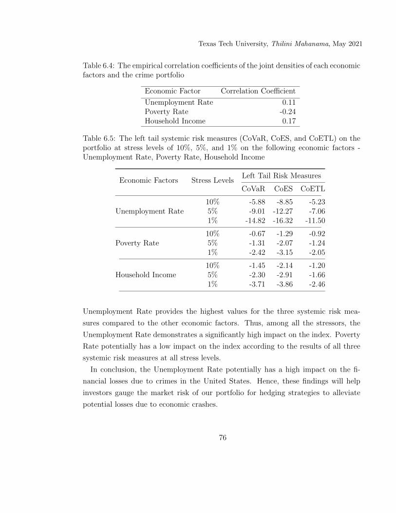
Texas Tech University, Thilini Mahanama, May 2021
Table 6.4: The empirical correlation coefficients of the joint densities of each economicfactors and the crime portfolio
Economic Factor Correlation Coefficient
Unemployment Rate 0.11Poverty Rate -0.24Household Income 0.17
Table 6.5: The left tail systemic risk measures (CoVaR, CoES, and CoETL) on theportfolio at stress levels of 10%, 5%, and 1% on the following economic factors -Unemployment Rate, Poverty Rate, Household Income
Economic Factors Stress LevelsLeft Tail Risk Measures
CoVaR CoES CoETL
Unemployment Rate10% -5.88 -8.85 -5.235% -9.01 -12.27 -7.061% -14.82 -16.32 -11.50
Poverty Rate10% -0.67 -1.29 -0.925% -1.31 -2.07 -1.241% -2.42 -3.15 -2.05
Household Income10% -1.45 -2.14 -1.205% -2.30 -2.91 -1.661% -3.71 -3.86 -2.46
Unemployment Rate provides the highest values for the three systemic risk mea-
sures compared to the other economic factors. Thus, among all the stressors, the
Unemployment Rate demonstrates a significantly high impact on the index. Poverty
Rate potentially has a low impact on the index according to the results of all three
systemic risk measures at all stress levels.
In conclusion, the Unemployment Rate potentially has a high impact on the fi-
nancial losses due to crimes in the United States. Hence, these findings will help
investors gauge the market risk of our portfolio for hedging strategies to alleviate
potential losses due to economic crashes.
76

Texas Tech University, Thilini Mahanama, May 2021
CHAPTER 7
DISCUSSION & CONCLUSION
Although over 69,000 tornadoes are recorded in NOAA Storm Data [3], we con-
sidered approximately 40,000 tornado events since not all of the tornado events had
measurements for all tornado variables (length, width, and losses). In section 4.3.2,
we analyzed the natural logarithm of the monthly property losses which resulted in
constant variance over the time series. In this study, we focused on states in Tornado
Alley on an ad hoc basis as they represent a disproportionately high frequency of
tornadoes [30].
Tornadoes are rated in [3] using an intensity-based scale known as the EF-scale
[1]. Moreover, the property loss caused by a tornado unequivocally depends on the
location and value of the real estate. For example, the damage costs due to a tornado
in an urban area might be significantly high even if the tornado has a low EF-Scale.
We implemented the MU algorithm for NMF to classify tornado data in [3], and
they exhibited a conspicuous classification underpinning property losses. We have
introduced a novel scale for tornado damages based on the property losses attributed
to them, the TPL-Scale (4.5).
Using simple linear regression analysis, we found the relationship between the
property loss and area affected by a tornado: Loss ∼√Area =
√Length ·Width
(i.e., Loss approximates to the geometric mean of path length and width). Then, we
employed a bivariate Gaussian copula approach to explore the underlying non-linear
dependence between ln(Area) and ln(Loss). However, the dependence coefficients
(copula parameters) between ln(Area) and ln(Loss) strongly vary with time and
geographical location. Thus, we trained the LSTM and shallow neural networks to
capture the long-term dependencies in the data set. Finally, we predicted monthly
property losses between 2020 and 2025 using the LSTM, and the expected volume
of property losses would amount to just under eight billion dollars over the next five
years (by 2025).
The approach of compensating for the property losses caused by tornadoes is a
two-fold process in the United States. For catastrophic tornadoes, the government
77

Texas Tech University, Thilini Mahanama, May 2021
coverage programs such as FEMA distribute fundings to local governments. For typ-
ical tornadoes, private insurance companies cover the tornado damage costs claimed
by their clients. We recovered the existence of these two risk assessment strate-
gies by learning a statistical manifold on probability distributions of property losses.
The smooth connection between the points in the manifold illustrates that there is no
single good enough distribution to describe all available property losses in [3]. There-
fore, we defined a measure of curvature on the manifold to estimate such volatilities
in property losses with respect to small changes in tornado path lengths and path
widths. However, there are few extremities in data that we failed to interpret using
the statistical manifold.
In this dissertation, chapter 3 and 4 addressed the risk assessment strategies of
tornadoes reported in the NOAA Storm Data [3]. We considered reported tornado
data as separate events and investigated the risk in terms of the property losses. Due
to the lack of reported occurrences in [3], the risk assessment methods discussed in
chapter 3 and 4 cannot be implemented for other types of natural disasters. There-
fore, we integrated the reported property losses in all 50 types of disasters in time
steps (in particular, two-week increments). Then, we utilized the temporal ordering
of financial losses for hedging the risk due to natural disasters in chapter 5.
As a result, we proposed the Natural Disasters Index, NDI (5.1), using the United
States as a model with property losses reported in NOAA Storm Data [3] between
1996 and 2018. In order to establish the NDI, we provided an evaluation framework
using three promising approaches: (1) option pricing, (2) risk budgeting, and (3)
stress testing.
We determined the fair values of the NDI options using a discrete-time GARCH
model with GH innovations and then simulated Monte Carlo averages to approxi-
mate call and put option prices (5.7),(5.8). The relationships among time to maturity,
strike price, and option prices help to construct and valuate insurance-type financial
instruments. Then, we disaggregated the cumulative risk attributed to natural dis-
asters to our equally-weighted portfolio (i.e., we investigated the risk contribution
of each type of natural disaster). The Std and ETL risk budgets for the NDI yield
that flood and flash flood are the main risk contributors in our portfolio. Finally, we
78

Texas Tech University, Thilini Mahanama, May 2021
assessed the performance of the NDI via a stress testing analysis using Max Temp
and PDSI as stressors. We found the stress on Max Temp significantly impacts the
NDI compared to that of the PDSI at the highest stress level (1%).
The proposed NDI is an attempt to address a financial instrument for hedging the
intrinsic risk induced by the property losses caused by natural disasters in the United
States. The main objective of the NDI is to forecast the degree of future systemic
risk caused by natural disasters. This information could forewarn the insurers and
corporations allowing them to transfer insurance risk to capital market investors.
Hence the issuance of the NDI will conspicuously help to bridge the gap between
the capital and insurance markets. While the NDI is specifically constructed for the
United States, it could be modified to calculate the risk in other regions or countries
using a data set comparable to NOAA Storm Data [3].
Following the financial management principles in the NDI, we proposed construct-
ing a portfolio that outlines the financial impacts of various types of crimes in the
United States. In order to that, we modeled the financial losses of crimes reported
by the Federal Bureau of Investigation using the annual cumulative property losses
due to property crimes and cybercrimes. Then, we backtested the index using VaR
models at different levels to find a proper model for implementing in evaluation pro-
cesses. As a result, we utilized ARMA(1,1)-GARCH(1,1) with Student’s t model to
evaluate the crime portfolio.
We presented the use of our portfolio on crimes through option pricing, risk bud-
geting, and stress testing. First, we provided fair values for European call and put
option prices (Figure 6.1 and 6.2) and implied volatilities (Figure 6.3) for our portfo-
lio. Second, we found the risk attributed to each type of crime based on tail risk and
center risk measures. Third, we evaluated the performance of our index for the eco-
nomic crisis by implementing stress testing. According to the findings, in the United
States, the Unemployment Rate potentially has a higher impact on the financial
losses due to the crimes incorporated in this study compared to the Poverty Rate
and Median Household Income. The findings, estimated option prices, risk budgets,
and systemic risk outlined in the portfolio will help investors with financial planning
on our portfolio.
79

Texas Tech University, Thilini Mahanama, May 2021
BIBLIOGRAPHY
[1] Storm Prediction Center,National Weather Service (NWS), National Oceanicand Atmospheric Administration (NOAA). The Enhanced Fujita Scale (EFScale), 2019.
[2] National Weather Service Reports, 2019.
[3] National Centers for Environmental Information (NCEI), National Oceanicand Atmospheric Administration (NOAA). Storm Events Database, availableat https://www.ncdc.noaa.gov/stormevents/.
[4] Sreelekshmy Selvin, R Vinayakumar, EA Gopalakrishnan, Vijay KrishnaMenon, and KP Soman. Stock price prediction using lstm, rnn and cnn-slidingwindow model. In 2017 international conference on advances in computing,communications and informatics (icacci), pages 1643–1647. IEEE, 2017.
[5] Inc. The MathWorks. Long Short-Term Memory Networks, Deep Learing Tool-box. Natick, Massachusetts, United State, 2019.
[6] Vyacheslav Lyubchich and YR Gel. Can we weather proof our insurance?Environmetrics, 28(2):e2433, 2017.
[7] Hiroko Tabuchi. 2017 Set a Record for Losses From Natural Disasters. It CouldGet Worse. The New York Times, 2018.
[8] Panos Varangis, Jerry Skees, and Barry Barnett. Weather indexes for devel-oping countries. Forest, 4:3–754, 2003.
[9] Maxx Dilley, Robert S Chen, Uwe Deichmann, Arthur L Lerner-Lam, andMargaret Arnold. Natural disaster hotspots: a global risk analysis. The WorldBank, 2005.
[10] Gregory Van der Vink, Richard M Allen, Jeffery Chapin, Morgan Crooks,W Fraley, Joshua Krantz, AnnMarie Lavigne, Andrew LeCuyer, Eugene KMacColl, WJ Morgan, et al. Why the united states is becoming more vul-nerable to natural disasters. Eos, Transactions American Geophysical Union,79(44):533–537, 1998.
80

Texas Tech University, Thilini Mahanama, May 2021
[11] Jesse E Bell, Claudia Langford Brown, Kathryn Conlon, Stephanie Herring,Kenneth E Kunkel, Jay Lawrimore, George Luber, Carl Schreck, Adam Smith,and Christopher Uejio. Changes in extreme events and the potential im-pacts on human health. Journal of the Air & Waste Management Association,68(4):265–287, 2018.
[12] Richard J Roth Sr and Howard Kunreuther. Paying the price: The status androle of insurance against natural disasters in the United States. Joseph HenryPress, 1998.
[13] Christopher M. Lewis and Kevin C. Murdock. The role of government contractsin discretionary reinsurance markets for natural disasters: Abstract. Journalof Risk and Insurance (1986-1998), 63(4):567, 12 1996.
[14] Zongxia Liang, Lin He, and Jiaoling Wu. Optimal dividend and reinsur-ance strategy of a property insurance company under catastrophe risk. arXivpreprint arXiv:1009.1269, 2010.
[15] Ngouffo Zangue and Jaures Poppo. Evaluating catastrophe risk and cat bondspricing methods. B.S. thesis, Universita Ca’Foscari Venezia, 2016.
[16] Howard Kunreuther. Mitigating disaster losses through insurance. Journal ofrisk and Uncertainty, 12(2-3):171–187, 1996.
[17] Philip T Ganderton, David S Brookshire, Michael McKee, Steve Stewart, andHale Thurston. Buying insurance for disaster-type risks: experimental evi-dence. Journal of risk and Uncertainty, 20(3):271–289, 2000.
[18] National Centers for Environmental Information (NCEI), National Oceanic andAtmospheric Administration (NOAA). Billion-Dollar Weather and ClimateDisasters: Overview, 2020.
[19] Adam B Smith and Jessica L Matthews. Quantifying uncertainty and vari-able sensitivity within the us billion-dollar weather and climate disaster costestimates. Natural Hazards, 77(3):1829–1851, 2015.
[20] Frank J Massey Jr. The kolmogorov-smirnov test for goodness of fit. Journalof the American statistical Association, 46(253):68–78, 1951.
[21] Ingwer Borg and Patrick JF Groenen. Modern multidimensional scaling: The-ory and applications. Springer Science & Business Media, 2005.
81

Texas Tech University, Thilini Mahanama, May 2021
[22] Daniel D. Lee and H. Sebastian Seung. Algorithms for non-negative matrixfactorization. In T. K. Leen, T. G. Dietterich, and V. Tresp, editors, Advancesin Neural Information Processing Systems 13, pages 556–562. MIT Press, 2001.
[23] Roger Nelsen. Properties and applications of copulas: A brief survey. Proc.1st Braz. Conf. on Stat. Modeling in Insurance and Finance, 01 2003.
[24] Barry J Barnett and Olivier Mahul. Weather index insurance for agricultureand rural areas in lower-income countries. American Journal of AgriculturalEconomics, 89(5):1241–1247, 2007.
[25] J David Cummins, David Lalonde, and Richard D Phillips. The basis risk ofcatastrophic-loss index securities. Journal of Financial Economics, 71(1):77–111, 2004.
[26] Claus Vorm Christensen and Hanspeter Schmidli. Pricing catastrophe insur-ance products based on actually reported claims. Insurance: Mathematics andEconomics, 27(2):189–200, 2000.
[27] Francesca Biagini, Yuliya Bregman, and Thilo Meyer-Brandis. Pricing of catas-trophe insurance options written on a loss index with reestimation. Insurance:Mathematics and Economics, 43(2):214–222, 2008.
[28] Walter Kielholz and Alex Durrer. Insurance derivatives and securitization:New hedging perspectives for the us cat insurance market. Geneva Papers onRisk and Insurance. Issues and Practice, pages 3–16, 1997.
[29] John D. Murphy. Storm data preparation. National Weather Service(NWS) instruction 10-1605, National Oceanic and Atmospheric Administra-tion (NOAA), 2018.
[30] National Centers for Environmental Information (NCEI), National Oceanicand Atmospheric Administration (NOAA). Tornado Alley, 2020.
[31] Tetsuya Theodore Fujita. Proposed characterization of tornadoes and hurri-canes by area and intensity (satellite and mesometeorology research projectreport 91). Chicago: University of Chicago, 119(5), 1971.
[32] Harold E Brooks. On the relationship of tornado path length and width tointensity. Weather and forecasting, 19(2):310–319, 2004.
82

Texas Tech University, Thilini Mahanama, May 2021
[33] Christian Schoelzel and Petra Friederichs. Multivariate non-normally dis-tributed random variables in climate research-introduction to the copula ap-proach. NPGeo, 15(5):761–772, 2008.
[34] Raushan Bokusheva. Improving the effectiveness of weather-based insurance:an application of copula approach. Institute for Environmental Decisions, 2014.
[35] Federal Bureau of Investigation Internet Crime Complaint Center. Crime inthe united states, 2019. 2020.
[36] Federal Bureau of Investigation United States Department of Justice. Crimein the united states, 2019. 2020.
[37] Federal Bureau of Investigation United States Department of Justice. Crimein the united states, 2011. 2020.
[38] Julie Josse, Jerome Pages, and Francois Husson. Multiple imputation in princi-pal component analysis. Advances in data analysis and classification, 5(3):231–246, 2011.
[39] M Serva, D Vergni, D Volchenkov, and A Vulpiani. Recovering geography froma matrix of genetic distances. Europhysics letters, 118(4):48003, 2017.
[40] Stanley T Birchfield and Amarnag Subramanya. Microphone array positioncalibration by basis-point classical multidimensional scaling. IEEE transactionson Speech and Audio Processing, 13(5):1025–1034, 2005.
[41] Florian Wickelmaier. An introduction to mds. Sound Quality Research Unit,Aalborg University, Denmark, 46(5):1–26, 2003.
[42] Eugene TY Lee. Choosing nodes in parametric curve interpolation. Computer-Aided Design, 21(6):363–370, 1989.
[43] Michael W Berry, Murray Browne, Amy N Langville, V Paul Pauca, andRobert J Plemmons. Algorithms and applications for approximate nonnegativematrix factorization. Computational statistics & data analysis, 52(1):155–173,2007.
[44] M. Shokrollahi and S. Krishnan. Non-negative matrix factorization and sparserepresentation for sleep signal classification. In 2013 35th Annual InternationalConference of the IEEE Engineering in Medicine and Biology Society (EMBC),pages 4318–4321, July 2013.
83

Texas Tech University, Thilini Mahanama, May 2021
[45] Richard A Johnson and Dean Wichern. Multivariate analysis. Wiley StatsRef:Statistics Reference Online, pages 1–20, 2014.
[46] Daniel D Lee and H Sebastian Seung. Learning the parts of objects by non-negative matrix factorization. Nature, 401(6755):788–791, 1999.
[47] Nacim Fateh Chikhi, Bernard Rothenburger, and Nathalie Aussenac-Gilles. Acomparison of dimensionality reduction techniques for web structure mining.In IEEE/WIC/ACM International Conference on Web Intelligence (WI’07),pages 116–119. IEEE, 2007.
[48] Zhong-Yuan Zhang. Nonnegative matrix factorization: Models, algorithmsand applications. In Data Mining: Foundations and Intelligent Paradigms:Volume 2: Statistical, Bayesian, Time Series and other Theoretical Aspects,volume 24 of Intelligent Systems Reference Library, pages 99–134. SpringerBerlin Heidelberg, Berlin, Heidelberg, 2012.
[49] Patrik O Hoyer. Non-negative matrix factorization with sparseness constraints.Journal of machine learning research, 5(Nov):1457–1469, 2004.
[50] Nicolas Gillis. The why and how of nonnegative matrix factorization. Regular-ization, Optimization, Kernels, and Support Vector Machines, 12, 01 2014.
[51] Serhat S Bucak and Bilge Gunsel. Incremental subspace learning via non-negative matrix factorization. Pattern recognition, 42(5):788–797, 2009.
[52] Andreas Janecek and Ying Tan. Iterative improvement of the multiplicativeupdate nmf algorithm using nature-inspired optimization. In 2011 SeventhInternational Conference on Natural Computation, volume 3, pages 1668–1672.IEEE, 2011.
[53] Chih-Jen Lin. On the convergence of multiplicative update algorithms fornonnegative matrix factorization. IEEE Transactions on Neural Networks,18(6):1589–1596, 2007.
[54] Inc. The MathWorks. Non-negative Matrix Factorization, Dimensionality Re-duction and Feature Extraction. Natick, Massachusetts, United State, 2019.
[55] David M Pozar. Microwave engineering. John Wiley & Sons, 2009.
[56] Christian Genest and Anne-Catherine Favre. Everything you always wantedto know about copula modeling but were afraid to ask. Journal of hydrologicengineering, 12(4):347–368, 2007.
84

Texas Tech University, Thilini Mahanama, May 2021
[57] Rogelio Salinas-Gutierrez, Arturo Hernandez-Aguirre, Mariano JJ Rivera-Meraz, and Enrique R Villa-Diharce. Using gaussian copulas in supervisedprobabilistic classification. In Soft Computing for Intelligent Control and Mo-bile Robotics, pages 355–372. Springer, 2010.
[58] Hamani El Maache and Yves Lepage. Spearman’s rho and kendall’s tau formultivariate data sets. Lecture Notes-Monograph Series, pages 113–130, 2003.
[59] Gregory A Fredricks and Roger B Nelsen. On the relationship between spear-man’s rho and kendall’s tau for pairs of continuous random variables. Journalof statistical planning and inference, 137(7):2143–2150, 2007.
[60] Abootaleb Shirvani and Dimitri Volchenkov. A regulated market under sanc-tions. on tail dependence between oil, gold, and tehran stock exchange index.Journal of Vibration testing and System Dynamic, 3(3):297–311, 2019.
[61] Rong-Gang Cong and Mark Brady. The interdependence between rainfall andtemperature: copula analyses. The Scientific World Journal, 2012.
[62] Workamaw P Warsido and Girma T Bitsuamlak. Synthesis of wind tunneland climatological data for estimating design wind effects: A copula basedapproach. Structural Safety, 57:8–17, 2015.
[63] Youssef Stitou, Noureddine Lasmar, and Yannick Berthoumieu. Copulas basedmultivariate gamma modeling for texture classification. In 2009 IEEE Interna-tional Conference on Acoustics, Speech and Signal Processing, pages 1045–1048.IEEE, 2009.
[64] Roger B Nelsen. Copulas and association. In Advances in probability distribu-tions with given marginals, pages 51–74. Springer, 1991.
[65] Shahrbanou Madadgar and Hamid Moradkhani. Drought analysis under cli-mate change using copula. Journal of hydrologic engineering, 18(7):746–759,2013.
[66] Andrew Gordon Wilson and Zoubin Ghahramani. Copula processes. In Pro-ceedings of the 23rd International Conference on Neural Information Process-ing Systems - Volume 2, NIPS’10, page 2460–2468, Red Hook, NY, USA, 2010.Curran Associates Inc.
85

Texas Tech University, Thilini Mahanama, May 2021
[67] C Piani and JO Haerter. Two dimensional bias correction of temperature andprecipitation copulas in climate models. Geophysical Research Letters, 39(20),2012.
[68] Daniel Berg and Henrik Bakken. A goodness-of-fit test for copulae based onthe probability integral transform. Preprint series. Statistical Research Reporthttp://urn. nb. no/URN: NBN: no-23420, 2005.
[69] Juan Carlos Rodriguez. Measuring financial contagion: A copula approach.Journal of empirical finance, 14(3):401–423, 2007.
[70] Andras Bardossy and Jing Li. Geostatistical interpolation using copulas. WaterResources Research, 44(7), 2008.
[71] George Casella and Roger L Berger. Statistical inference, volume 2. DuxburyPacific Grove, CA, 2002.
[72] Daniel Berg. Copula goodness-of-fit testing: an overview and power compari-son. The European Journal of Finance, 15(7-8):675–701, 2009.
[73] Marius Hofert, Ivan Kojadinovic, Martin Machler, and Jun Yan. Elements ofcopula modeling with R. Springer, 2019.
[74] Jun Yan et al. Enjoy the joy of copulas: with a package copula. Journal ofStatistical Software, 21(4):1–21, 2007.
[75] Gianfausto Salvadori, Carlo De Michele, Nathabandu T Kottegoda, and RenzoRosso. Extremes in nature: an approach using copulas. Springer Science &Business Media, 2007.
[76] DianQing Li, XiaoSong Tang, ChuangBing Zhou, and Kok-Kwang Phoon. Un-certainty analysis of correlated non-normal geotechnical parameters using gaus-sian copula. Science China Technological Sciences, 55(11):3081–3089, 2012.
[77] Christian Meyer. The bivariate normal copula. Communications in Statistics-Theory and Methods, 42(13):2402–2422, 2013.
[78] Chris AJ Klaassen, Jon A Wellner, et al. Efficient estimation in the bivariatenormal copula model: normal margins are least favourable. Bernoulli, 3(1):55–77, 1997.
86

Texas Tech University, Thilini Mahanama, May 2021
[79] Alex Graves and Jurgen Schmidhuber. Framewise phoneme classification withbidirectional lstm and other neural network architectures. Neural networks,18(5-6):602–610, 2005.
[80] Felix A Gers, Nicol N Schraudolph, and Jurgen Schmidhuber. Learning precisetiming with lstm recurrent networks. Journal of machine learning research,3(Aug):115–143, 2002.
[81] Sepp Hochreiter and Jurgen Schmidhuber. Long short-term memory. Neuralcomputation, 9(8):1735–1780, 1997.
[82] Thomas Fischer and Christopher Krauss. Deep learning with long short-termmemory networks for financial market predictions. European Journal of Oper-ational Research, 270(2):654–669, 2018.
[83] Alex Graves, Abdel-rahman Mohamed, and Geoffrey Hinton. Speech recogni-tion with deep recurrent neural networks. IEEE international conference onacoustics, speech and signal processing, pages 6645–6649, 2013.
[84] Hasim Sak, Andrew W Senior, and Francoise Beaufays. Long short-term mem-ory recurrent neural network architectures for large scale acoustic modeling.Fifteenth Annual Conference of the International Speech Communication As-sociation, 2014.
[85] Felix A Gers, Jurgen Schmidhuber, and Fred Cummins. Learning to forget:Continual prediction with lstm. Neural Comput, 1999.
[86] Xiang Li, Ling Peng, Xiaojing Yao, Shaolong Cui, Yuan Hu, Chengzeng You,and Tianhe Chi. Long short-term memory neural network for air pollutant con-centration predictions: Method development and evaluation. Environmentalpollution, 231:997–1004, 2017.
[87] Xiaolei Ma, Zhimin Tao, Yinhai Wang, Haiyang Yu, and Yunpeng Wang. Longshort-term memory neural network for traffic speed prediction using remote mi-crowave sensor data. Transportation Research Part C: Emerging Technologies,54:187–197, 2015.
[88] Yongxue Tian and Li Pan. Predicting short-term traffic flow by long short-termmemory recurrent neural network. In 2015 IEEE international conference onsmart city/SocialCom/SustainCom (SmartCity), pages 153–158. IEEE, 2015.
87

Texas Tech University, Thilini Mahanama, May 2021
[89] Xiangyun Qing and Yugang Niu. Hourly day-ahead solar irradiance predictionusing weather forecasts by lstm. Energy, 148:461–468, 2018.
[90] R. Fu, Z. Zhang, and L. Li. Using lstm and gru neural network methods fortraffic flow prediction. In 2016 31st Youth Academic Annual Conference ofChinese Association of Automation (YAC), pages 324–328, Nov 2016.
[91] Niek Tax, Ilya Verenich, Marcello La Rosa, and Marlon Dumas. Predictive busi-ness process monitoring with lstm neural networks. In International Conferenceon Advanced Information Systems Engineering, pages 477–492. Springer, 2017.
[92] Inc. The MathWorks. Time Series Forecasting Using Deep Learnin. Natick,Massachusetts, United State, 2019.
[93] Rob J Hyndman and Anne B Koehler. Another look at measures of forecastaccuracy. International journal of forecasting, 22(4):679–688, 2006.
[94] A Alexandre Trindade, Abootaleb Shirvani, and Xiaohan Ma. A socioeconomicwell-being index. arXiv preprint arXiv:2001.01036, 2020.
[95] NCEI. U.S. Climate Extremes Index (CEI). National Centers for Environmen-tal Information (NCEI), National Oceanic and Atmospheric Administration(NOAA), accessed by 2019.
[96] Wayne C Palmer. Meteorological drought, volume 30. US Department of Com-merce, Weather Bureau, 1965.
[97] Karin L Gleason, Jay H Lawrimore, David H Levinson, Thomas R Karl, andDavid J Karoly. A revised us climate extremes index. Journal of climate,21(10):2124–2137, 2008.
[98] Matthew J Menne, Claude N Williams Jr, and Russell S Vose. The us historicalclimatology network monthly temperature data, version 2. Bulletin of theAmerican Meteorological Society, 90(7):993–1008, 2009.
[99] Russell S Vose, Scott Applequist, Mike Squires, Imke Durre, Matthew J Menne,Claude N Williams Jr, Chris Fenimore, Karin Gleason, and Derek Arndt. Im-proved historical temperature and precipitation time series for us climate divi-sions. Journal of Applied Meteorology and Climatology, 53(5):1232–1251, 2014.
[100] Richard R Heim Jr. A review of twentieth-century drought indices used inthe united states. Bulletin of the American Meteorological Society, 83(8):1149–1166, 2002.
88

Texas Tech University, Thilini Mahanama, May 2021
[101] William M Alley. The palmer drought severity index: limitations and assump-tions. Journal of climate and applied meteorology, 23(7):1100–1109, 1984.
[102] Thomas R Heddinghaus and Paul Sabol. A review of the palmer droughtseverity index and where do we go from here. In Proc. 7th Conf. on AppliedClimatology, pages 242–246. American Meteorological Society Boston, MA,1991.
[103] Fischer Black and Myron Scholes. The pricing of options and corporate liabili-ties. In World Scientific Reference on Contingent Claims Analysis in CorporateFinance: Volume 1: Foundations of CCA and Equity Valuation, pages 3–21.World Scientific, 2019.
[104] Dilip B Madan, Frank Milne, and Hersh Shefrin. The multinomial optionpricing model and its brownian and poisson limits. The Review of FinancialStudies, 2(2):251–265, 1989.
[105] Simon R Hurst, Eckhard Platen, and Svetlozar Todorov Rachev. Option pricingfor a logstable asset price model. Mathematical and computer modelling, 29(10-12):105–119, 1999.
[106] Peter Carr and Liuren Wu. Time-changed levy processes and option pricing.Journal of Financial economics, 71(1):113–141, 2004.
[107] Richard A Bell. Option pricing with the extreme value distributions. Universityof London, London, 2006.
[108] Sven Klingler, Young Shin Kim, Svetlozar T Rachev, and Frank J Fabozzi.Option pricing with time-changed levy processes. Applied financial economics,23(15):1231–1238, 2013.
[109] Svetlozar Rachev, Frank J Fabozzi, Boryana Racheva-Iotova, and AbootalebShirvani. Option pricing with greed and fear factor: The rational financeapproach. arXiv preprint arXiv:1709.08134, 2017.
[110] Abootaleb Shirvani, Frank J Fabozzi, and Stoyan V Stoyanov. Option pricingin an investment risk-return setting. arXiv preprint arXiv:2001.00737, 2020.
[111] Abootaleb Shirvani, Yuan Hu, Svetlozar T Rachev, and Frank J Fabozzi. Op-tion pricing with mixed levy subordinated price process and implied probabilityweighting function. The Journal of Derivatives, 28(2):47–58, 2020.
89

Texas Tech University, Thilini Mahanama, May 2021
[112] J.C. Duan. The garch option pricing model. Mathematical Finance, 5:13–32,1995.
[113] P. Blaesild. The two-dimensional hyperbolic distribution and related distri-butions with an application to johannsen’s bean data. Mathematical Finance,68:251–263, 1981.
[114] H. U. Gerber and E. S. W. Shiu. Option pricing by esscher transforms. Trans-actions of the Society of Actuaries, 46:99–191, 1994.
[115] C. Chorro. Option pricing for garch-type models with generalized hyperbolicinnovations. Quantitative Finance, 12(7):1079–1094, 2012.
[116] G. Chow and M. Kritzman. Risk budgets. Journal of Portfolio Management,pages 56–60, 2001.
[117] R. B. Litterman. Hot spots and hedges. Journal of Portfolio Management,pages 52–75, 1996.
[118] S. Maillard, T. Roncalli, and J. Teiletche. On the properties of equallyweightedrisk contributions portfolios. Journal of Portfolio Management, pages 52–75,2010.
[119] B. Peterson and K. Boudt. Component var for a non-normal world. Journalof Risk, pages 78–81, 2008.
[120] K. Boudt, P. Carl, and B. G. Peterson. Asset allocation with conditionalvalue-at-risk budgets. Journal of Risk, 15(3):39–68, 2013.
[121] Tobias Adrian and Markus K Brunnermeier. Covar. Technical report, NationalBureau of Economic Research, 2011.
[122] Giulio Girardi and A Tolga Ergun. Systemic risk measurement: Multivariategarch estimation of coVaR. Journal of Banking & Finance, 37(8):3169–3180,2013.
[123] Carlo Acerbi and Dirk Tasche. Expected shortfall: a natural coherent alterna-tive to value at risk. Economic notes, 31(2):379–388, 2002.
[124] Georg Mainik and Eric Schaanning. On dependence consistency of covar andsome other systemic risk measures. Statistics & Risk Modeling, 31(1):49–77,2014.
90

Texas Tech University, Thilini Mahanama, May 2021
[125] A. Biglova, S. Ortobelli, and F.J. Fabozzi. Portfolio selection in the presenceof systemic risk. Journal of Asset Management, 15:285–299, 2014.
[126] Peter Whittle. The analysis of multiple stationary time series. Journal of theRoyal Statistical Society: Series B (Methodological), 15(1):125–139, 1953.
[127] Tim Bollerslev. Generalized autoregressive conditional heteroskedasticity.Journal of econometrics, 31(3):307–327, 1986.
[128] Philippe Jorion. Value at risk: the new benchmark for managing financial risk.The McGraw-Hill Companies, Inc., 2007.
[129] Olli Nieppola et al. Backtesting value-at-risk models. 2009.
[130] Manuela Braione and Nicolas K Scholtes. Forecasting value-at-risk under dif-ferent distributional assumptions. Econometrics, 4(1):3, 2016.
[131] F. Black and M. Scholes. The pricing of options and corporate liabilities. TheJournal of Political Economy, 81:637–654, 1973.
[132] R.C. Merton. Theory of rational option pricing. The Bell Journal of Economicsand Management, 4:141–183, 1973.
[133] Benoit Mandelbrot and Howard M Taylor. On the distribution of stock pricedifferences. Operations research, 15(6):1057–1062, 1967.
[134] Peter K Clark. A subordinated stochastic process model with finite variancefor speculative prices. Econometrica: journal of the Econometric Society, pages135–155, 1973.
[135] Sato Ken-Iti. Levy processes and infinitely divisible distributions. Cambridgeuniversity press, 1999.
[136] Simon R Hurst, Eckhard Platen, and Svetlozar T Rachev. Subordinated marketindex models: A comparison. Financial Engineering and the Japanese Markets,4(2):97–124, 1997.
[137] Abootaleb Shirvani, Svetlozar T Rachev, and Frank J Fabozzi. Multiple subor-dinated modeling of asset returns: Implications for option pricing. EconometricReviews, pages 1–30, 2020.
[138] Ole E. Barndorff-Nielsen. Normal inverse gaussian distributions and stochasticvolatility modelling. Scandinavian Journal of Statistics, 24(1):1–13, 1997.
91

Texas Tech University, Thilini Mahanama, May 2021
[139] P. Carr and D. Madan. Option valuation using the fast fourier transform.Journal of Computational Finance, 2:61—-73, 1998.
[140] Thilini V Mahanama and Abootaleb Shirvani. A natural disasters index. arXivpreprint arXiv:2008.03672, 2020.
[141] Yuan Hu, Svetlozar T Rachev, and Frank J Fabozzi. Modelling crypto assetprice dynamics, optimal crypto portfolio, and crypto option valuation. arXivpreprint arXiv:1908.05419, 2019.
92