Low temperature studies for the sulphuric acid decomposition ...

Low temperature studies for the sulphuric

acid decomposition step in the HyS and SI

thermochemical cycles

Thesis submitted to the Department of Chemical and Biological Engineering, University of Sheffield, for the Degree of Doctor of

Philosophy (PhD)

by

Moisés Alfonso Romero González, B.Eng(Hons)

Department of Chemical and Biological Engineering

University of Sheffield

July 2013

Chemical & Biological Engineering

II

Abstract

Hydrogen is a promising element for the transition from fossil fuels, even

though the majority of industrial hydrogen production methods are not carbon-

neutral. There are, however, alternatives which could produce this CO2 free fuel

on a massive scale. In particular, thermochemical cycles, including the Hybrid

Sulfur (HyS) and Sulfur-Iodine (SI) cycles, which share a common sulphuric acid

decomposition step. This project continues the work done by Shaw (2008),

which involved the acquisition of experimental data relevant to the production of

Hydrogen in the sulphur family of thermochemical cycles. This also lays the

framework needed to continue the thermodynamic calculations needed for the

design of equipment relevant to the SO2/O2/H2O separation. The model was

developed simultaneously with the design of the next generation equilibrium still

that was able to incorporate in-situ analysis. Several technical design milestones

were achieved in the process, including the development of a sapphire liquid

gas cell, a glass reinforced single pass 10 cm Zinc Selenide gaseous cell,

several iterations of Raman Spectroscopy probes with ranging capabilities for

different purposes, mostly high pressures and temperatures. It was also

confirmed that with the low temperature separation approach, materials become

an important factor for the success or failure of the process.

Based on the results comparison between the calculations of the

Mathematica® model, the GFE model, the available experimental data and

general tendencies in the literature, it is concluded that the calculations, as well

as the experimental techniques used throughout this project, are successful for

their purpose, which is the aiding of equipment design for the HyS and SI cycle,

Further efforts can be done to implement this model into process modelling

software.

III

Acknowledgements

I would like to thank Prof. Ray Allen for his continuous guidance, motivation

and encouragement; to Dr. Rachael Elder for her everlasting patience and to Dr.

Dmitriy Kuvshinov, Dr. Geof Priestman, Prof. Will Zimmerman, Dr. Rile Ristic and

Dr. Jordan MacInnes, for the stimulating discussions that helped shape this

project.

I would like to acknowledge the support and training received from the

brilliant technical staff in the Chemical Engineering Department, Adrian Lumby,

Andy Patrick, Stuart Richards, Mike O’Meara, Dave Palmer, Oz McFarlane, Mark

McIntosh, Usman Younis and to the very fond memory of the late Clifton Wray.

Finally, I’d like to thank everyone that was involved in this project for all the

support they have given me throughout almost 4 years of continuous problem

solving, in and out of the lab: my friends in Tampico, Veracruz and other parts of

Mexico, my friends in the Chemical Engineering Department, in Sheffield, in

London, my 3 brothers and their families (Nico, Bola and Samail) and most

importantly, my parents (Nicolas and Carmela).

Without them, this amazing journey would have been impossible.

IV

Indivisa Manent!

(Remain Undivided)

Vince in Bono Malum

(Overcome Evil with Good)

Rerum Cognoscere Causas

(To Discover and Understand)

V

Table of Contents

Abstract ................................................................................................................................... II

Acknowledgements ................................................................................................................... III

Table of Contents ..................................................................................................................... V

Nomenclature .......................................................................................................................... XI

Chapter 1 - Introduction

Table of Contents ........................................................................................................................ 1

1.1 Overview and General Remarks .............................................................................................. 2

1.2 Aim .......................................................................................................................................... 3

1.3 Background ............................................................................................................................ 4

1.4 Outline ..................................................................................................................................... 5

1.5 Energy and The Hydrogen Economy ....................................................................................... 7

1.5.1 Hydrogen National Programs ..................................................................................... 9 1.5.2 Hydrogen: Energy Carrier ......................................................................................... 11

1.6 H2 Production routes ............................................................................................................. 12

1.7 Summary ............................................................................................................................... 13

Chapter 1 References ........................................................................................................................ 14

Chapter 2 – Literature Review on the H2SO4 decomposition

Table of Contents .................................................................................................................... 19

2.1 Background to Thermochemical Cycles ................................................................................ 20

2.2 SI Cycle ................................................................................................................................. 20

2.3 HyS Cycle ............................................................................................................................. 22

2.3.1 Example Flow sheets in the HyS Cycle .................................................................... 23 2.3.2 SO2 Electrolysers ..................................................................................................... 25

2.4 Acid decomposition background ........................................................................................... 26

2.4.1 SI and HyS flowsheets ............................................................................................. 27

2.5 Decomposition Section Development .................................................................................... 27

2.6 Decomposer Design .............................................................................................................. 29

2.7 Material Development ............................................................................................................ 30

2.8 Catalyst Development ........................................................................................................... 31

VI

2.9 Previous work with sulphur species solutions ........................................................................ 32

2.9.1 Binary Mixtures ........................................................................................................ 33

2.10 Work on O2 solutions ............................................................................................................. 33

2.10.1 Tromans Solubility .................................................................................................... 34 2.10.2 Germanium Oxidation .............................................................................................. 34

2.11 Previous work with sulphuric Acid ......................................................................................... 35

2.12 Summary ............................................................................................................................... 36


Chapter 3 VLE Theoretical Background

Chapter 3. Table of Contents ................................................................................................. 43

3.1 Overview ............................................................................................................................... 44

3.2 The equilibrium condition ....................................................................................................... 45

3.2.1 Gibbs fundamental Equation .................................................................................... 47

3.3 Non idealities: Activity and Fugacity ....................................................................................... 49

3.3.1 Gas Fugacity and the Fugacity coefficient ................................................................ 49 3.3.2 Molality .................................................................................................................... 50 3.3.3 Gibbs Free Energy Change at Equilibrium ................................................................ 50 3.3.4 Activity Coefficient .................................................................................................... 52 3.3.5 Approaches for Activity Coefficient Calculation ........................................................ 52

3.4 Solubility of Gases ................................................................................................................. 56

3.4.1 The Bunsen coefficient α ......................................................................................... 56 3.4.2 The Ostwald Coefficient L ........................................................................................ 56 3.4.3 The weight solubility ................................................................................................. 57 3.4.4 Henry’s Law Constant ............................................................................................. 57

3.5 Reacting Equilibrium: Electrolytes .......................................................................................... 57

3.5.1 Phase and Chemical Equilibrium .............................................................................. 57

3.6 Approach to Equilibrium Calculations .................................................................................... 58

3.6.1 Reaction Constant Calculation ................................................................................. 58

3.7 Gibbs Free Energy Minimization Technique ........................................................................... 66

3.7.1 Gibbs Procedural calculation ................................................................................... 68

3.8 Summary ............................................................................................................................... 69

References for Chapter 3 ................................................................................................................... 70

VII

Chapter 4 Thermodynamic Modelling

Chapter 4 Table of Contents ................................................................................................... 74

4.1 Overview ............................................................................................................................... 75

4.2 Justification ........................................................................................................................... 75

4.3 Sulphuric Acid Equilibrium ..................................................................................................... 76

4.3.1 H2SO4 dissociation ................................................................................................... 76

4.4 Problem Set Up ..................................................................................................................... 82

4.4.1 Reaction Equations .................................................................................................. 83

4.5 Equilibrium equations ............................................................................................................ 84

4.5.1 Vapour-liquid Equilibrium Equations ......................................................................... 84 4.5.2 Reaction Equations .................................................................................................. 85 4.5.3 Fugacity Coefficients ................................................................................................ 86 4.5.4 Activity Coefficients .................................................................................................. 86 4.5.5 Selection of Fugacity and Activity Coefficients Methods ........................................... 87

4.6 Summary of Code Changes .................................................................................................. 87

4.6.1 Molecular Interaction Parameters ............................................................................. 88 4.6.2 Guessing of initial values .......................................................................................... 88 4.6.3 Secant Method ........................................................................................................ 89 4.6.4 Iterative behaviour of VLE model .............................................................................. 89 4.6.5 Reaction Rate Constants ......................................................................................... 90 4.6.6 Electroneutrality ....................................................................................................... 90

4.7 Sample Calculations: HSC and Mathematica ........................................................................ 90

4.8 Discussion ............................................................................................................................. 93

4.9 Summary ............................................................................................................................... 94


Chapter 5 Experimental Design

Table of Contents .................................................................................................................... 100

Background ............................................................................................................................ 105

5.1 Overview ............................................................................................................................. 105

5.2 Aim ...................................................................................................................................... 105

5.3 Previous Equilibrium Still Designs ........................................................................................ 106

5.3.1 Mark I and Mark II .................................................................................................. 108 5.3.1 Mark III ................................................................................................................... 110 5.3.2 Experimental Procedure ......................................................................................... 115 5.3.3 Spatial Thermal Uniformity ..................................................................................... 116 5.3.4 PID Damping ......................................................................................................... 117 5.3.5 Sample Flashing .................................................................................................... 118

5.4 Requirements: Visualisation, Solids and Phase determination ............................................. 120

5.4.1 Flow visualisation ................................................................................................... 120

VIII

5.4.2 Solid Formation: SO2 Clathrate Hydrate ................................................................. 121 5.4.3 Aqueous and SO2 phase determination ................................................................. 122

5.5 Thermal-switch Incident ...................................................................................................... 123

5.5.1 Root Cause Analysis .............................................................................................. 123 5.5.2 Mark III Follow-up .................................................................................................. 124

Mark IV Design ...................................................................................................................... 126

5.6 Aim ...................................................................................................................................... 126

5.7 Material Considerations ....................................................................................................... 126

5.8 Pressure Vessel Calculations ............................................................................................... 127

5.8.1 Operating Pressure ................................................................................................ 128 5.8.2 Allowable Stress .................................................................................................... 128

5.9 Thermal Properties ............................................................................................................... 129

5.9.1 Preliminary thermal calculations ............................................................................. 129 5.9.2 Problem set-up ...................................................................................................... 130 5.9.3 Lumped System Analysis for transient heat conduction Rig Design ....................... 130

5.10 Equipment & Instrumental Design ........................................................................................ 132

5.11 Spectroscopic theoretical background ................................................................................ 133

5.11.1 Infrared spectroscopy ............................................................................................ 133 5.11.2 Raman spectroscopy ............................................................................................. 134 5.11.3 Raman Spectrometer ............................................................................................. 134 5.11.4 FTIR Spectrometer ................................................................................................. 139 5.11.5 Auto Titrator ........................................................................................................... 141

5.12 Infrared Materials ................................................................................................................. 141

5.12.1 Silicon .................................................................................................................... 141 5.12.2 Germanium ............................................................................................................ 144 5.12.3 Zinc Selenide ......................................................................................................... 145

5.13 Chemical Inertness ............................................................................................................... 146

5.14 Infrared Developments ........................................................................................................ 147

5.14.1 Gas Cell ................................................................................................................. 147 5.14.2 Full ATR Configuration Results ............................................................................... 150 5.14.3 Liquid Cell .............................................................................................................. 152

5.15 Mark IV Additional Considerations ....................................................................................... 153

5.15.1 Weight and Dead Volume ...................................................................................... 153 5.15.2 Germanium ATR Design ........................................................................................ 154 5.15.3 Thermal Uniformity ................................................................................................. 157

5.16 Summary ............................................................................................................................. 159

References for Chapter 5 ................................................................................................................. 160

Chapter 6 Results & Discussion

Table of Contents ............................................................................................................................ 164

List of Figures .................................................................................................................................. 165

IX

List of Tables ................................................................................................................................... 167

6.1 Overview ............................................................................................................................. 168

6.2 Aim ...................................................................................................................................... 168

6.3 Data Acquisition .................................................................................................................. 171

6.4 Sample Analysis .................................................................................................................. 172

Results .................................................................................................................................. 174

6.5 Dissolved Sulphur Dioxide ................................................................................................... 175

6.5.1 Binary Data ............................................................................................................ 175 6.5.2 Ternary Data .......................................................................................................... 178 6.5.3 Isomolar Calculation Method .................................................................................. 178 6.5.4 Temperature Effects ............................................................................................... 188 6.5.5 Quaternary Data ..................................................................................................... 189 6.5.6 Effect of Acid species............................................................................................. 189

6.6 Dissolved Oxygen ................................................................................................................ 191

6.6.1 Salting Out Effect ................................................................................................... 193

6.7 Sulphites and other species ................................................................................................ 194

6.8 Uncertainty Analysis ............................................................................................................ 197

6.8.1 Species Mass Addition .......................................................................................... 197 6.8.2 Gas Uncertainty ..................................................................................................... 200 6.8.3 Iodometry Uncertainty ............................................................................................ 202 6.8.4 Gas Chromatography ............................................................................................ 203

6.9 Summary ............................................................................................................................. 205

Chapter 6 References 207

Chapter 7 Conclusions & Future Work

Table of Contents .................................................................................................................. 210

7.1 Overview ............................................................................................................................. 211

7.2 Discussion ........................................................................................................................... 212

7.2.1. Gibbs Free Energy Calculations ............................................................................. 212 7.2.2. Acid threshold in HyS and SI operation .................................................................. 214

7.3 Suggested Future Work ...................................................................................................... 214

7.2.3. Spectroscopy ........................................................................................................ 215 7.2.4. Prismatic In-situ Acquisition ................................................................................... 215 7.2.5. Conical In-situ Acquisition ...................................................................................... 215 7.2.6. Implementation of the Model .................................................................................. 216

7.4 Summary ............................................................................................................................. 218


X

Appendixes

Appendix A. Experimental Procedure

Appendix B. LabVIEW Program

Appendix C. HSC Calculation Example

Appendix D. Mathematica Calculations

Appendix E. Macros in Visual Basic

Appendix F. Publications

Appendix G. Technical Drawings

Consolidated Reference List

XI

Nomenclature Symbols

a Activity

a Parameter signifying the hard core size of molecules for the Nakamura equation of state l mole-1

A Helmholtz energy J AI Interfacial area m2

b Parameter signifying the attractive force strength for the Nakamura equation of state l atm mole-1

B Second virial coefficient cm3 mole-1

c Constant for the Nakamura equation of state l mole-1 Cp Heat capacity J mol-1 K-1 d0 Density g cm-3

Dw Dielectric constant of water E Electrode potential Volts Et Threshold energy for water splitting eV f Fugacity atm, bar G Gibbs free energy J

iG Partial molar Gibbs free energy J mol-1 GE Gibbs excess free energy J

EiG Partial molar Gibbs excess free energy J mol-1

GR Residual Gibbs energy J oΔG Standard Gibbs free energy J mol-1

oih Molar enthalpy of pure i J mol-1

hG Gas specific constant m3 kmol-1 hT Gas parameter for salting out equation m3 kmol-1 K-1 H Enthalpy kJ mol-1 Hij Henry’s constant atm kg mole-1

ofΔH Standard enthalpy of formation kJ mol-1 ΔHºrxn Standard enthalpy of reaction kJ mol-1

I Ionic strength mol (kg H2O)-1

I Current Amps k Boltzmann’s constant (see table of constants) J K-1 k Reaction rate constant Specified in text kH Reciprocal of Henry’s constant mole kg-1 atm-1 ksc Salting out coefficient m3 kmol-1 K Equilibrium constant

Kp Equilibrium constant in terms of partial pressure of gases

KT Thermodynamic equilibrium constant ovL Ostwald coefficient

m Molal concentration mol (kg H2O)-1

2SOm Molal concentration of SO2 moles SIV (kg H2O)-1

XII

2Om Molal concentration of O2 moles O2 (kg H2O)-1 mH2O Mass of water kg M Extensive thermodynamic property

iM Partial molar M of component i Me Metal ion MW Molecular weight of water (see Appendix C) g mole-1

n Moles of species moles NA Avogadro’s number (see table of constants) mol-1 p Partial pressure bar, atm P Pressure bar, atm Pi Partial pressure of species i bar, atm R Universal gas constant (see table of constants) R Electrical Resistance Ohms sº Gas solubility in pure water Molality s Gas solubility in salt solution Molality S Entropy J K-1 SIV Total dissolved sulphur dioxide SIV

0 Initial concentration of SIV t Time seconds T Absolute temperature K Tn Normal boiling point K U Internal energy J vi Molar volume of species i l mole-1

iv Partial molar volume of species i l mole-1 v−∞ Partial molar volume at infinite dilution l mole-1 v Stoichiometric coefficient V Volume ml, l olV Volume of pure liquid ml, l

xi Mole fraction of species i in the liquid y Mole fraction Z Compressibility factor

XIII

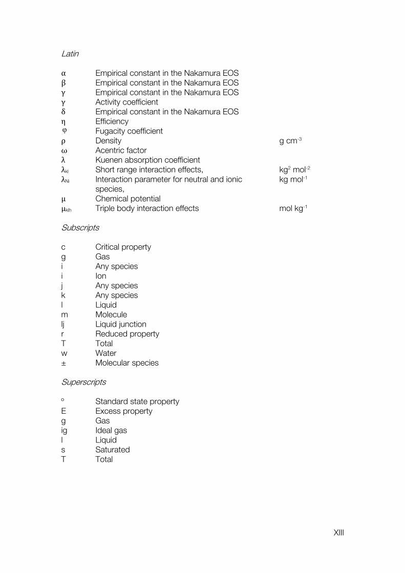
Latin α Empirical constant in the Nakamura EOS β Empirical constant in the Nakamura EOS γ Empirical constant in the Nakamura EOS γ Activity coefficient δ Empirical constant in the Nakamura EOS η Efficiency φ Fugacity coefficient ρ Density g cm-3 ω Acentric factor λ Kuenen absorption coefficient λkl Short range interaction effects, kg2 mol-2 λNi Interaction parameter for neutral and ionic

species, kg mol-1 μ Chemical potential μklh Triple body interaction effects mol kg-1

Subscripts c Critical property g Gas i Any species i Ion j Any species k Any species l Liquid m Molecule lj Liquid junction r Reduced property T Total w Water ± Molecular species Superscripts º Standard state property E Excess property g Gas ig Ideal gas l Liquid s Saturated T Total

Chapter 1

Introduction

1

Chapter 1

Table of Contents

Table of Contents ....................................................................................................................... 1

1.1 Overview and General Remarks ............................................................................................... 2

1.2 Aim 3

1.3 Background ............................................................................................................................. 4

1.4 Outline ..................................................................................................................................... 5

1.5 Energy and The Hydrogen Economy ........................................................................................ 7

1.5.1 Hydrogen National Programs ..................................................................................... 9 1.5.2 Hydrogen: Energy Carrier ........................................................................................ 11

1.6 H2 Production routes .............................................................................................................. 12

1.7 Summary ............................................................................................................................... 13



2

1.1 Overview and General Remarks

This work involves the characterization of a vapour liquid equilibrium

system both experimentally and mathematically. This system is ideally represented

by an enclosed vessel that includes conditions relevant to the sulphur family of

thermochemical cycles. The studied media consists of a mixture of chemical

species (described below) in both liquid and gaseous phases. These, in turn,

achieve chemical and phase equilibrium at a certain temperature and pressure.

This equilibrium behaviour is best described with the theory of weak aqueous

electrolyte thermodynamics.

The multicomponent gas-liquid mixture at hand contains sulphur dioxide,

oxygen, water and traces of sulphuric acid, which is a very important solution in

the separation step involving the decomposition of H2SO4. The sulphur family of

thermochemical cycles, namely the Hybrid Sulphur cycle (HyS) and the Sulphur

Iodine (SI) cycle, share this common sulphuric acid step, which leads to products

that need to be effectively separated for the efficiency of the cycle not to be

compromised.

As part of an international effort to research renewables and the gradual

substitution for fossil fuels, the University of Sheffield has contributed towards the

advancement of thermochemical cycles, especially towards the research of the

H2SO4 decomposition step. In this group, thermochemical cycles have been

investigated within four main approaches:

High temperature membrane separation via ceramic membranes

Low temperature poly-sulphonated ionomer membranes

Experiments using ionic liquids

Classic, low temperature vapour-liquid equilibria separation

While the former three have been investigated by other authors in this

University, efforts presented here are concerned with the latter, low temperature

approach. The hypothesis is that a high-temperature stream of products (after the


3

sulphuric acid decomposition step) would be lowered to the 30 to 50 °C range,

and then separated by conventional means (absorption columns or flash units),

which agrees with the optimal separator conditions by the work of Jeong & Kazimi

in their HyS optimised flowsheet. (Jeong Y.H., 2005).

To date, no rigorous study of the equilibrium between sulphur dioxide,

oxygen and water exists, let alone including sulphuric acid. On the other hand,

several studies with subsystems (e.g., SO2-H2O, SO3-H2SO4-H2O, etc.) have been

detailed. The aim of this work is to obtain thermodynamic data fully characterizing

solubility behaviours of this mixture, as well as advancing spectroscopic

knowledge towards it. This thesis continues the work of Dr. Andrew Shaw, which

laid an experimental basis for this required data, starting with binary SO2-O2

mixtures, followed by a rigorous ternary model containing SO2, O2 and H2O).

In this chapter, hydrogen will be presented as a justification for this

project. Hydrogen, an alternative to fossil fuels, sustains the motivation behind this

work. The research objectives and the thesis outline will be presented, before

briefly describing the hydrogen economy concept, some national programs

highlighting H2 production, before going on to Thermochemical Cycles and acid

decomposition on the next chapter.

1.2 Aim

To our knowledge, no full representation of the vapour liquid equilibrium of

sulphur dioxide, oxygen, water and sulphuric acid has been reported in literature.

Even further, rigorous thermodynamic modelling for this system and information

required to develop it, is scarce. According to Duigou et al. (2007), both the SI and

the HyS cycles can only be viable if they achieve two important criteria:

competitive cost and successful large scale demonstration.

If both cycles are to be competitive, they need to get as close as possible

to the maximum theoretical efficiency. These numbers, depending on the

methodology, oscillate between 40 and 50%, and it has been discussed often,


4

according to Elder and Allen (2009). As in all engineering processes, it is standard

practice to focus on the separation equipment, which amounts to a considerable

percentage of the energy of the cycle, as well as its capital costs. If one is to

succeed in developing detailed engineering for the cycles, it is imperative to obtain

accurate thermodynamic data that will aid in the design of the aforementioned

separation equipment. This work focuses on that effort.

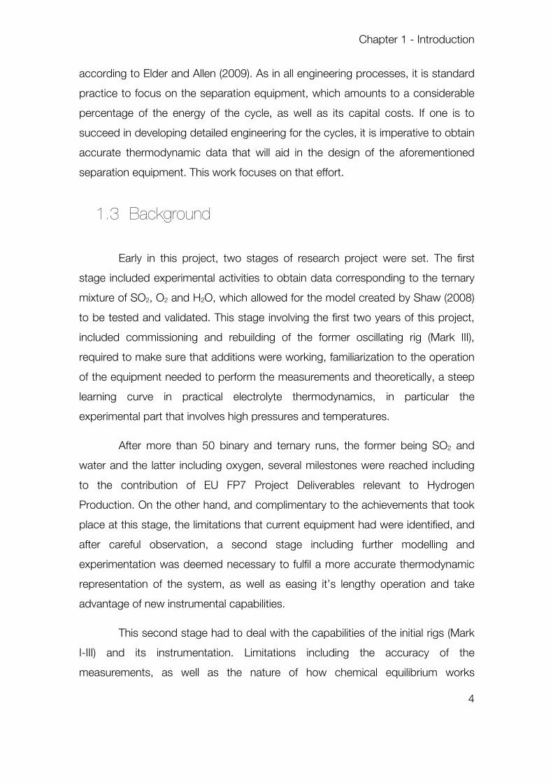
1.3 Background

Early in this project, two stages of research project were set. The first

stage included experimental activities to obtain data corresponding to the ternary

mixture of SO2, O2 and H2O, which allowed for the model created by Shaw (2008)

to be tested and validated. This stage involving the first two years of this project,

included commissioning and rebuilding of the former oscillating rig (Mark III),

required to make sure that additions were working, familiarization to the operation

of the equipment needed to perform the measurements and theoretically, a steep

learning curve in practical electrolyte thermodynamics, in particular the

experimental part that involves high pressures and temperatures.

After more than 50 binary and ternary runs, the former being SO2 and

water and the latter including oxygen, several milestones were reached including

to the contribution of EU FP7 Project Deliverables relevant to Hydrogen

Production. On the other hand, and complimentary to the achievements that took

place at this stage, the limitations that current equipment had were identified, and

after careful observation, a second stage including further modelling and

experimentation was deemed necessary to fulfil a more accurate thermodynamic

representation of the system, as well as easing it’s lengthy operation and take

advantage of new instrumental capabilities.

This second stage had to deal with the capabilities of the initial rigs (Mark

I-III) and its instrumentation. Limitations including the accuracy of the

measurements, as well as the nature of how chemical equilibrium works


5

(discussed in Chapters 3 and 4), made necessary the development of new

experimental approaches, dealing with spectroscopic methods and the

development of a new rig (Mark-IV - see Chapter 5). This, in turn, brought new

research objectives that proved the most challenging, and ultimately the most

productive.

All in all, the commissioning of the Mark-IV and the acquisition of data with

it culminates the second stage of this project, bringing to conclusion this summary

of research objectives:

To fully characterize both ternary and quaternary mixtures and their

thermodynamic data, both with experiments and calculations;

To design an apparatus capable of providing solubility data for a broader

range of conditions, in order to enhance current separation knowledge within

the sulphur thermochemical cycles;

To be able to cope with more dangerous and corrosive media (such as the

addition of dilute sulphuric acid at high temperatures and pressures in this

multicomponent mixture of sulphur dioxide, oxygen and water)

The capability to subject equilibrium mixtures to test in a quicker, better and

safer way.

To pave the way to rigorous modelling in thermochemical flow sheets,

relevant to H2 production.

For its better understanding, the development of this work must then be

described methodically. An outline is presented in the next section.

1.4 Outline

The introductory part starts with Chapter One, where the research

background is explained, along with general remarks about the hydrogen research

field as well as an outline of the thesis structure and its research objectives.


6

Chapter Two tackles thermochemical cycles, mainly the sulphuric acid

decomposition, and a thorough analysis for different hydrogen plant alternatives,

including a discussion on the sulphuric acid decomposition step and its recent

developments.

Chapter Three lays the theoretical foundation needed to deal with vapour

liquid equilibrium, equations of state and aqueous electrolyte solutions.

Chapter Four covers the development of a rigorous vapour-liquid

equilibrium model containing equations describing a system containing SO2, O2 in

an aqueous sulphuric acid solution. This model largely takes from the

methodology laid down by Zemaitis et al. (1986).

Chapter Five describes the design and engineering of the new

experimental apparatus, as well as a brief description of the analytic techniques

intended for it.

Chapter Six presents the tests performed and the results obtained from

the apparatuses used in this project, with a focus on solubility diagrams, as well as

the compilation of ternary data gathered from the first apparatus. It contains a

discussion of the results gathered, contrasting the experimental and the

calculations, along with the concluding remarks gathered from the comparison

between the model and the experiments,

Chapter 7 contains the conclusions drawn from this project, a summary of

findings and finally the recommended future work available for this particular

research project.

Finally, included at the end of this dissertation are appendixes that contain

calculations relevant to the design of the reactor, as well as parameters useful for

the study of this work and experimental procedures that were essential, but not

directly related to the results obtained. In the next section, some important

aspects of the hydrogen economy are addressed.


7

1.5 Energy and The Hydrogen Economy

It is unarguable that the fuel for technology advancement in a modern

society is energy and its consumption; at least on a large scale (Jorgenson, 1984).

Energy not only is related to technological growth, but also to quality the of life, the

economy, productivity; even obesity (Drewnowski and Specter, 2004). This is an

example of how energy is intimately close to human life. There’s no question

about the finite nature of fossil fuels, one of the examples being the peak in oil

production in the UK, shown in Figure 1.

Figure 1. Oil peak in the United Kingdom (Hirsch et al., 2005).

Since the oil crisis in the ‘70’s, and the price spike in 2008, a renewed

interest in energy sustainability emerged. It is clear that the problem that arises

from energy demand and production must be addressed in the future. Although it

is important to state that as we deplete hydrocarbons in general (oil, natural gas,

shales and tar sands) new reserves are found, it is clear that the nature of these

resources is finite, and it is clear that their extraction and processing is detrimental

to the environment (Dudley, 2012).

After the oil price shocks of the 1970’s, oil as a share of primary energy

has been reduced from 48% in 1973 to 39% in 1985, and BP predicts that it will


8

continue to be reduced to a further 28% by 2030. However, by 2030, renewables

will account for 6% of the global primary energy by 2030. Hydrogen would be

included in the ideal diversified energy portfolio of the future (BP, 2012). Current

forecasts predict that increasing costs of energy production will deem today’s

technologies insufficient (Moriarty and Honnery, 2009). Not only do the economic

costs of fossil fuels rise, but also the environmental impact, especially in

developing countries. A future energy portfolio including hydrogen could alleviate

some of the demand problems in the future. This is all but a new idea, dating to

the XIXth century.

The concept of the hydrogen economy is a term coined by John O’Mara

Bockris in his speech at the General Motors Technical Centre in 1970, and

reported in the section 2.20 of the conference proceedings, “On Methods For the

Large Scale Production of Hydrogen From Water”. It is fundamentally a developed

energy system based only on hydrogen. It arose as a response to the

environmental concerns that fossil fuel combustion and depletion posed to the

scientific community and the energy crisis in the mid-seventies, but as Weston

puts it, from the seventies to how we presently got here four decades later is a

study worthy of many volumes (Weston, 1992).

Hydrogen is clean in terms of pollutants created by its combustion (only

H2O); and it can also be produced from water, a very abundant resource in the

planet. This is one of the reasons why this system could solve the greenhouse

effect and regional environmental problems.

For the sole purpose of creating consciousness about this proposed

economy, the International Association for Hydrogen Energy (IAHE)1 was

established in Florida, U.S., starting the International Journal of Hydrogen Energy

(IJHE) and holding biennial World Hydrogen Energy Conferences (WHEC), helping


9

the developing concept to be thoroughly studied. By 1980, the hydrogen

economy was fully theorized and explained as the transition of non-renewable

fuels into a hydrogen-based economy; with its transportation and storage

schemes, industrial and domestic usage and appropriate materials to deliver. The

hydrogen economy has been fed by research in over 40 countries, with some of

them including the scheme in their energy policies (e.g., U.S., Iceland, Japan,

Germany) (Goltsov and Veziroglu, 2001). Selected programs are briefly discussed

in next section.

1.5.1 Hydrogen National Programs

Many nations have pursued the know-how to make the transition to a

hydrogen economy more approachable. Some examples are provided below. This

list is not exhaustive, but it is a recap of some of the national hydrogen programs

that amounted to a relevant budget figure.

In Japan, the government-funded WE-NET Program has already

researched hydrogen-combustion technologies, and they presented a prototype

hydrogen fuelled burner operating at 1700 °C, with efficiencies of 60%. Hydrogen

was produced by a 90% efficient SPEM electrolysis (Hijikata, 2002). Prospective

R&D will comprise a short, mid and long-term result analysis, for them to be

practically applied throughout 1993-2030. These objectives are proposed:

200,000 m3 of hydrogen storage; 50,000 m3 of cryogenic material storage, 30 to

50 kW fuel cells, 100 kW H2 Diesel engines, 30 Nm3/h H2 refuelling, and finally H2

large-scale utilization (Mitsugi et al., 1998). Public demonstrations are yet to be

developed.

In Germany, a H2 mobility Initiative plans to bring infrastructure for the HE

implementation. Germany holds 70% of all fuel cell demonstrations in Europe. The

Ministry of Foreign Trade and Investment has a clear intention of propelling the

fuel-cell industry, where more than 350 companies and institutes are operating in

this matter, particularly in the North-Rhine Westphalia region (Pastowski and


10

Grube, 2010). The annual growth for fuel cells is expected to be of more than 200

MW from 2015. Partners include among others, Daimler, Linde, Shell, Total and

EnBW. Germany also collaborated with Saudi Arabia in HySolar (Abaoud and

Steeb, 1998), a program ended in 1995 where they built a Solar H2 plant near

Riyadh, funded with $4.7M split 50-50 between mainly the King Abdulaziz City for

Science and Technology, and the German Aerospace Research establishment

(DLR).

Canada entered a joint research program with Europe, the Euro-Quebec

project (Drolet et al., 1996), where research has been applied to importing

schemes between them, proving that importing H2(l) from Canada can be

successful, especially in the iron and transportation industry; as well in developing

a prospective massive transportation infrastructure between the two. More

recently, the WHEC 2012 was held in Toronto, where companies from different

parts of the world showcased their achievements, including profitability for the first

quarter. This is significant, as it shows that hydrogen technologies can overcome

negative economic climate if the market is there, even a niche one.

Iceland, on the other hand, is an example of a complete commitment

towards a Hydrogen Economy. Several institutions, including the transportation

industry, commodity companies, multi-national companies, universities and the

government have formed a commitment to a full hydrogen implementation.

Currently, there are various programs including the SMART-H2, H-SHIP and

PREPAR-H2; which are studying experimentally the hydrogen introduction in

Iceland at a social, technical and economical level. The transition is planned to be

fully completed in 2050, facilitated by partners such as DaimlerChrysler, Norsk

Hydro and Shell Hydrogen. Some of the technologies could be integrated with

hydroelectric power. In 2007, Hydropower powered almost 73.4% of electricity

generation in the country, with a prospective addition of >700 MW to the grid

(Orkustofnun, 2007).

In Australia, ACIL Tasman and Parsons Brinckeroff prepared a National

Hydrogen Study, in 2007, appointed by the Department of Industry, Tourism and


11

Resources. It contains an assessment of the role of hydrogen in Australia, plus

recommendations that would lay the foundation for their inclusion in the HE.

Veziroglu and several other researchers have compiled the status of

Hydrogen Energy in a thorough manner, rendering optimistic results; mentioning

enterprises that have already started to commercialize hydrogen production

technology, expertise and energy systems; including automotive systems,

electrolysis units, battery technologies and hazard studies concerning H2

transportation (Veziroğlu and Takahashi, 1990) (Momirlan and Veziroglu, 2002)

(EHA, 2012). There is a stable scientific community developing new ideas for the

H2 transition, including prospects that go beyond 2100 (Goltsov and Veziroglu,

2001). A comprehensive economic evaluation of Hydrogen national programs has

been presented by Khamis, et.al. (2011), whereas Dunn (2002) showed an

interesting political narrative for Hydrogen in his publication. In the recent WHEC

2012, held in Toronto, several hydrogen fuel cell companies achieved profitability

for the first time since their inception. This further thrusts hydrogen from niche-

market towards mass market positioning.

1.5.2 Hydrogen: Energy Carrier

Hydrogen is the most abundant element in the galaxy, and only forms

water when lit. Hydrogen is not found naturally, and it is a light, colourless gas with

a density of 0.0899 kg/Nm , and a boiling point of only 20.39 °K (Haynes and

Lide, 2010). The energy stored in 1 kg of H2 is approximately equivalent to 2.75

kg of gasoline, and it has the most dense energy / mass ratio, compared to other

common fuels, although storage remains to be efficiently addressed. However,

technological obstacles that were thought to be limiting for the development of the

hydrogen economy are quickly fading away as technologies achieve their original

benchmark goals.

These factors, along with clean burning and availability; make H2 a

promising energy carrier, which, contrary to energy source, it is only a means of


12

transporting and distributing energy for its consumption, according to the ISO

13600:1997 definition 2 (ISO, 1997). This is an important distinction. Petrol, or

solar energy, are examples of energy sources; whereas hydrogen and electricity

are examples of energy carriers.

1.6 H2 Production routes

Figure 2. Diagram of the main H2 production routes (Stolten, 2010).

A number of technologies are available for hydrogen production which

can be categorized as renewable and non-renewables (Taylor, 2006), some of

them are represented in Figure 2. The main difficulty of hydrogen production is

that it continues to be coupled with some non-renewable fuels or processes, like

natural gas or gasoline reforming. As of this moment, the most popular industrial

method to produce hydrogen comes from reforming hydrocarbons with steam,

especially natural gas which contains methane. The EIA gave a rough estimate of

hydrogen production costs using different prospective technologies, these are

shown below in Table 1.


13

Table 1. Estimate Hydrogen Production Costs. (J.Joosten, 2008).

In this EIA publication dated August 2008, it was clearly shown that the most

capacity could be achieved by thermochemical cycles. These are not limited to

nuclear energy; concentrated solar could also be used as an alternative source.

1.7 Summary

If the Hydrogen Economy is to be achieved, vast quantities of hydrogen

are required to be competitive with conventional fuels, and some of the current

production technologies are difficult to scale industrially. In this work,

thermochemical cycles have been selected for its potential to produce massive

amounts of hydrogen if coupled with nuclear or solar sources, using waste heat

from the fission processes or in solar tower concentrators. These are addressed in

the next chapter.

14

Chapter 1 References

ABAOUD, H. & STEEB, H. 1998. The German-Saudi HYSOLAR program. International Journal of Hydrogen Energy, 23, 445-449.

DREWNOWSKI, A. & SPECTER, S. 2004. Poverty and obesity: the role of energy density and energy costs. The American Journal of Clinical Nutrition, 79, 6-16.

DROLET, B., GRETZ, J., KLUYSKENS, D., SANDMANN, F. & WURSTER, R. 1996. The euro-québec hydro-hydrogen pilot project [EQHHPP]: demonstration phase. International Journal of Hydrogen Energy, 21, 305-316.

DUDLEY, B. 2012. BP statistical review of world energy.

DUIGOU, A. L., BORGARD, J.-M., LAROUSSE, B., DOIZI, D., ALLEN, R., EWAN, B. C., H. PRIESTMAN, G., ELDER, R., DEVONSHIRE, R., RAMOS, V., CERRI, G., SALVINI, C., GIOVANNELLI, A., DE MARIA, G., CORGNALE, C., BRUTTI, S., ROEB, M., NOGLIK, A., RIETBROCK, P.-M., MOHR, S., DE OLIVEIRA, L., MONNERIE, N., SCHMITZ, M., SATTLER, C., MARTINEZ, A. O., DE LORENZO MANZANO, D., CEDILLO ROJAS, J., DECHELOTTE, S. & BAUDOUIN, O. 2007. HYTHEC: An EC funded search for a long term massive hydrogen production route using solar and nuclear technologies. International Journal of Hydrogen Energy, 32, 1516-1529.

DUNN, S. 2002. Hydrogen futures: toward a sustainable energy system. International Journal of Hydrogen Energy, 27, 235-264.

EHA. 2012. EHA March Newsletter [Online]. Available: http://www.h2euro.org/category/publications/newsletters/newsletters-2012/eha-newsletter-march-2012.

ELDER, R. & ALLEN, R. 2009. Nuclear heat for hydrogen production: Coupling a very high/high temperature reactor to a hydrogen production plant. Progress in Nuclear Energy, 51, 500-525.

GOLTSOV, V. A. & VEZIROGLU, T. N. 2001. From hydrogen economy to hydrogen civilization. International Journal of Hydrogen Energy, 26, 909-915.

HAYNES, W. M. & LIDE, D. R. 2010. CRC Handbook of Chemistry and Physics: A Ready-Reference Book of Chemical and Physical Data, Taylor & Francis Group.

15

HIJIKATA, T. 2002. Research and development of international clean energy network using hydrogen energy (WE-NET). International Journal of Hydrogen Energy, 27, 115-129.

HIRSCH, R., BEZDEK, R. & WENDLING, R. Peaking of world oil production. Proceedings of the IV International Workshop on Oil and Gas Depletion, 2005. 19-20.

ISO 1997. ISO 13600:1997. 2- Definitions.

J.JOOSTEN, P. G., A. KYDES, J.D.MAPLES 2008. The Impact of Increased Use of Hydrogen on Petroleum Consumption and Carbon Dioxide Emissions. 1 ed. Washington, D.C. U.S. 20585: Energy Information Administration, U.S.DOE.

JEONG Y.H., M. S. K., K.J. HOHNHOLT, AND B. YILDIZ, 2005. Optimization of the Hybrid Sulfur Cycle for Hydrogen Generation. MIT–Nuclear Clear Energy and Sustainability (NES) PROGRAM, 004.

JORGENSON, D. W. 1984. The Role of Energy in Productivity Growth. The American Economic Review, 74, 26-30.

KHAMIS, I. 2011. An overview of the IAEA HEEP software and international programmes on hydrogen production using nuclear energy. International Journal of Hydrogen Energy, 36, 4125-4129.

MITSUGI, C., HARUMI, A. & KENZO, F. 1998. WE-NET: Japanese hydrogen program. International Journal of Hydrogen Energy, 23, 159-165.

MOMIRLAN, M. & VEZIROGLU, T. N. 2002. Current status of hydrogen energy. Renewable and Sustainable Energy Reviews, 6, 141-179.

MORIARTY, P. & HONNERY, D. 2009. Hydrogen's role in an uncertain energy future. International Journal of Hydrogen Energy, 34, 31-39.

PASTOWSKI, A. & GRUBE, T. 2010. Scope and perspectives of industrial hydrogen production and infrastructure for fuel cell vehicles in North Rhine-Westphalia. Energy Policy, 38, 5382-5387.

SHAW, A. C. 2008. The simultaneous solubility of sulphur dioxide and oxygen in water for the hybrid sulphur thermochemical cycle. Ph.D. Doctoral Thesis, University of Sheffield.

STOLTEN, D. 2010. Hydrogen and Fuel Cells: Fundamentals, Technologies and Applications, John Wiley & Sons.

16

TAYLOR, M. 2006. Improvement of the Sulphur-Iodine cycle through the addition of ionic liquids. M.Phil, University of Sheffield.

VEZIROĞLU, T. N. & TAKAHASHI, P. K. Hydrogen energy progress VIII :

proceedings of the 8th World Hydrogen Energy Conference, Honolulu and Waikoloa, Hawaii, U.S.A., 22-27 July 1990. In: VEZIROĞLU, T. N. & TAKAHASHI,

P. K., eds., 1990 New York :. Pergamon Press.

WESTON, K. C. 1992. Energy Conversion, West Publishing Company.

ZEMAITIS, J. F., CLARK, D. M., RAFAL, M. & SCRIVINER, N. C. 1986. Handbook of Aqueous Electrolyte Thermodynamics, New York, AIChE.

18

Chapter 2

Literature Review on the H2SO4

decomposition

19

Chapter 2.

Table of Contents

Chapter 2. Table of Contents ................................................................................................. 19

2.1 Background to Thermochemical Cycles ................................................................................ 20

2.2 SI Cycle ................................................................................................................................ 20

2.3 HyS Cycle ............................................................................................................................. 22

2.3.1 Example Flow sheets in the HyS Cycle .................................................................... 23 2.3.2 SO2 Electrolysers ..................................................................................................... 25

2.4 Acid decomposition background .......................................................................................... 26

2.4.1 SI and HyS flowsheets ............................................................................................ 27

2.5 Decomposition Section Development ................................................................................... 27

2.6 Decomposer Design ............................................................................................................. 29

2.7 Material Development ........................................................................................................... 30

2.8 Catalyst Development ........................................................................................................... 31

2.9 Previous work with sulphur species solutions ....................................................................... 32

2.9.1 Binary Mixtures ........................................................................................................ 33

2.10 Work on O2 solutions ............................................................................................................ 33

2.10.1 Tromans Solubility ................................................................................................... 34 2.10.2 Germanium Oxidation .............................................................................................. 34

2.11 Previous work with sulphuric Acid ......................................................................................... 35

2.12 Summary .............................................................................................................................. 36

Chapter 2 References ....................................................................................................................... 37

Chapter 2 – Literature Review on the H2SO4 Decomposition

20

2.1 Background to Thermochemical Cycles

In thermochemical cycles, water is split to H2 and O2 via a series of reactions,

while intermediate species are kept inside the cycle. As heat can be directly used and

the electrode potential lowered, the efficiency could be potentially enhanced to

commercial levels. This group has been involved with the SI and the HyS cycles, which

are presented in this chapter, along with important aspects that lead to the literature

relevant to the separation.

2.2 SI Cycle

The sulphur family of cycles was jointly developed by General Atomics,

Westinghouse and JRC (Funk, 1976). The SI cycle is a promising combination if

coupled with nuclear heat (Elder and Allen, 2009). It consists of three steps: the Bunsen

reaction, the Sulphuric Acid Decomposition, and the Hydroiodic Acid Decomposition.

The overall reactions occur as follows:

2 2( ) 2 ( )

2 2 ( ) 2 4 2 ( )

9 16

(2 10 8 ) ( 4 )

g l

l l

I SO H O

HI H O I H SO H O

Reaction 1

( ) 2 2 ( )(2 ) ( )g lHI H I Reaction 2

1 2 4 2 2 4 ( ) 2 ( )( 4 ) ( ) (4 )l lL H SO H O H SO H O Reaction 3

2 4 ( ) 2 4 ( )( ) ( )l gH SO H SO Reaction 4

2 4 ( ) 3 ( ) 2 ( )( ) ( ) ( )g g gH SO SO H O Reaction 5

13 ( ) 2 ( ) 22( ) ( )g gSO SO O Reaction 6

General Atomics developed the classification used in this work, consisting of

three sections. The first reaction is called the Bunsen reaction, an exothermic and


21

spontaneous reaction (if ranging from 20 – 100 °C); where water reacts with molecular

iodine and sulphur dioxide, that in certain concentrations, happen to produce two liquid

sulphuric and hydroiodic acid-rich phases, that are immiscible. The phase containing

the hydroiodic acid is called the HIx phase, due to the average of polyiodide formation

that occur inside it. The entire cycle is shown on Figure 1.

Figure 1. Schematic representation of the SI Cycle, with temperature profiling of the reactions. (E. Funk, 2001)

The second section, the so-called HIx step, is the most critical step in the cycle.

It occurs when the hydrogen iodide decomposes and concentrates to produce H2.

Further, H2O, I2 and SO2 are recycled in the system (O'Keefe et al., 1982). This is

shown above. The third section is the sulphuric acid decomposition, after which the

system of interest in this project is generated.

Efficiencies of this cycle, calculated by several publications (O'Keefe et al.,

1982, Ewan and Allen, 2005, Elder and Allen, 2009, Atkin, 2009), are in the ranges of

51%, without considering estimates from flow sheets; that is, taking into consideration

Equation 1,


22

2 @25 )

*

H O CH

WQ

Equation 1

where H is the enthalpy of formation of liquid water at ambient temperature,

Q and W are the heat and work requirements of the cycle and η* is the efficiency of the

heat to work conversion system, taken as 0.5 (Vitart et al., 2006).

From the set of reactions shown above, the upper bound of this efficiency,

calculated from the reversible heat and work requirements of the reactions, can be

estimated to be 51%. However, a refinement of the estimation, taking into account a

more detailed flow sheet along with plausible values of components efficiencies such as

pumps or compressors, leads to a value between 34% and 37%, depending on the

optimization assumed for heat recovery in the HIx Section.

Work at this department has been done to optimize flow sheets with the

software ProSimPlus®, estimating improvements up to 40%, using different dewatering

parameters, according to Elder (2005). Other work including flow sheet optimization,

from the original GA design, include research from Özturk (1995) and Huang and

T.Raissi (2005), using ideal and Peng-Robinson models respectively.

2.3 HyS Cycle

The HyS Cycle, known also as the Westinghouse Cycle, is a hybrid

thermochemical cycle, as electrolysis is used for the purpose of generating hydrogen,

this was originally developed by Brecher and Wu (1977) while working at

Westinghouse. The main reactions are shown below:

0.232 2 2 4 2

700 122 4 2 2 2

2 V

C

SO H O H SO H

H SO SO H O O

Reaction 7

The main advantage of this cycle is that, compared to normal water electrolysis

requiring a potential barrier of 1.23 V; the potential barrier for this first reaction is one


23

fifth only, with an exact voltage of 0.17 V needed. This theoretically lowers the power

required for operation of industrial electrolysers (Atkin, 2009, Ewan and Allen, 2005).

Originally, the energy sources aimed to satisfy the heat requirements of this

cycle were nuclear in nature; but recent research has shown that solar heliostats or

parabolic troughs can be used to produce the large amounts of heat required for the

process.

The focus in this cycle is mainly targeted at electrolyser development, since it is

the first step in the cycle and it is a particularly useful point of research in industrial

applications. It is also important to mention that according to Jeong & Kazimi (2005) the

acid electrolysis is the limiting step in this cycle.

Studies have shown that an electrolyser unit operating in the 500-600 mV per

cell can lead to a predicted efficiency of more than 50%, superior to all other cycles.

Research by Ewan and Allen (2005) even showed theoretical increases of up to 60%.

Analysis of the economic aspects of the cycle give an approximate $1.60 USD per H2

kilogram for a mature technology coupled with a nuclear plant, but since then prices

have changed according to recent data, e.g. Miller et al. (2012) considers a milestone

to achieve USD $2/gge ($2-4 dispensed). Summers and co-workers (2005) point out

that there are still some obstacles, e.g. current density, operating lifetime and moderate

capital cost.

2.3.1 Example Flow sheets in the HyS Cycle

The most up-to-date work in flow sheet optimization was done at MIT, with

contributions and comments from partners involved in the project. Other modifications

have focused on equipment design, rather than rearranging the whole process. The

work is shown in the next page, for clarity purposes.


24

Figure 2. Flow sheet developed by Jeong & Kazimi, et.al. (2005)


25

Current work at the Massachusetts Institute of Technology diverted focus on

the HyS cycle and started working on electrolyser technologies, and their coupling with

nuclear power (High Temperature Steam Electrolysers, HTSE); while the Westinghouse

Corporation already bet the future of Hydrogen on the HyS Cycle (Lahoda, 2010).

Although funding has decreased in the last couple of years, research is still being done

on a smaller scale and hopes of funding remain for thermochemical H2. In the following

sections, some related research is discussed.

2.3.2 SO2 Electrolysers

In the Westinghouse original design, the electrolyser unit has two chambers

separated by the electrolysing membrane, where hydrogen occurs at the cathode,

while SO2 is converted to sulphuric acid at the anode, following a scheme represented

in Figure 3:

Figure 3. The original electrolyser set-up, designed at Westinghouse. (Lu and Ammon, 1982)


26

More modern developments include a membrane electrode assembly, MEA;

obtaining lower cell resistance in return. The current density at a specific voltage in a

cell depends on the operating PT conditions; the composition and the concentration of

both the anolyte and catholyte.

The Westinghouse original benchmark of obtaining 500 mA/cm2 was achieved

by Staser, Gorensek and Summers (2009) with a 0.6V current; however, this was done

with concentrated sulphur dioxide. The optimal performance with dilute sulphur dioxide

concentrations has not been satisfactory yet. This milestone, if reached, would reduce

the electrolyser area by 60%, largely decreasing capital costs.

Particular attention has been brought to the research being presently done by

Yildiz et.al (2007), where high temperature electrocatalytic materials have been of

interest; viz, conducting oxide surfaces for enhanced activity and durability. These

materials will prove to be useful for the decomposition stages of the cycles, a materials

section is discussed in sections 2.7, 5.7 and 5.12.

2.4 Acid decomposition background

As mentioned previously, sulphuric acid decomposition is common to the two

most researched thermochemical cycles for hydrogen production: the SI and the HyS

cycles, although it is iterated slightly differently in each technology. In this group, a brief

review of the decomposition section developments was conducted by Atkin in his

doctoral dissertation (2009), however, since then a number of publications related to

the sulphuric acid step have been presented both in refereed papers, as well as

conferences where thermochemical cycles play a role as part of the hydrogen

production track, e.g. the ICH2P or WHEC conferences. It is worth mentioning again a

summary of the many advantages associated with the sulphur cycles, namely:

Non-volatile price of the end product, regardless of relatively high capital

costs associated

A massive reduction of greenhouse gas emissions throughout the

lifespan of a large scale H2 thermochemical plant.


27

Industrial capacities, high output for mass market demand,

complimentary to renewable hydrogen generation.

Lower capital costs compared to conventional electrolyser technologies.

Compatible with both nuclear and solar energy sources

Sulphur is cheap and abundant

Further benefits and cost reduction could be reached in the long term.

According to a report presented by TIAX LLC, the average HyS production costs will be

USD $5.68 in 2015 and USD $3.85 in 2025 (Kromer et al., 2011). Nonetheless, it is

necessary to indicate the technical challenges that remain in current research. These

aspects of this H2SO4 decomposition section will be presented below.

2.4.1 SI and HyS flowsheets

It is important to mention that although the development between the SI and

the HyS had stemmed in parallel, it is not to say that the interest is equal for both.

Disadvantages regarding the capital cost for iodine feedstock and process solid

difficulties somewhat hindered the SI cycle flow sheet development. This is why,

throughout this H2SO4 chapter, a preference to present selected conditions relevant to

the Hybrid Sulphur Cycle are discussed more than SI flowsheets, even if the

decomposition section chemistry remains with key similarities between both processes.

2.5 Decomposition Section Development

A great deal of research has been directed at this step in the SI and HyS

cycles. The sulphuric acid industry has helped in acquiring the know-how to tackle

some of the technical challenges present. The proposed steps, according to the

original cycle proposed by Westinghouse and included in flowsheets in the seminal

work of Öztürk and colleagues (Öztürk et al., 1995); consist of concentrating sulphuric

acid through a series of flashing equipment, starting from low operating pressures.

Then, it is dehydrated, before SO3 is decomposed into SO2. This decomposition is only

partial, for undecomposed sulphur trioxide is recombined with water, which allows


28

recovering of its heat content (Vitart et al., 2006). As stated by Vitart, for this particular

section, several tasks had to be met. Catalyst endurance needed to be analysed, as

well as a conceptual decomposer that could tackle the challenges posed by these

harsh conditions. Since the mid-2000’s, several additions and optimizations have been

included in the original flowsheet by Bilgen (1995), and these other technical challenges

have been met.

10 years later, Huang and co-workers (2005) analysed and optimized the work

carried out by Öztürk (1995) and added some changes to the original flow sheets,

achieving energy efficiencies of 76%. Some calculations were based on chemical

equilibrium for the sulphuric acid decomposition, where these assumptions were made:

Simple phase gases were considered ideal,

Liquid phases were considered to be real solutions

Henry’s Law to predict behaviour of sulphur dioxide and water;

These assumptions were used to optimize the Bilgen’s flowsheet, arguably,

“without compromising efficiency or process” feasibility, lowering acid decomposition

temperatures down to 500 °C. This has important implications for this work: this is a

simplification that accounts for a strong argument against the accuracy of the flow

sheets, as there is no indication of electrolyte behaviour or non-idealities in the gas

phases.

Figure 4. Huang’s improved sulphuric acid decomposition step, originally conceived by Bilgen (2005). HySYS was used to enhance the original flow sheet. Three flow sheets were studied in that particular

research, simplifications used are stated above.


29

On behalf of the sulphur-iodine side, in Japan, a week long demonstration of

the cycle was conducted, but not in a closed-loop configuration, leaving questions

about effects on recycling and reaction completion. In the SI cycle, sulphuric acid is

reduced and then the remaining oxygen and SO2 are reacted in the Bunsen section,

leaving hydroiodic and sulphuric acid, whose densities are sufficiently different for them

to be separated easily. As stated in an feasibility analysis about the sulphuric acid

decomposition from the Sandia National Laboratories (Perret, 2011), in the SI cycle,

extractive distillation using phosphoric acid and iodine recovery remain an issue.

On the side of the Hybrid Sulphur side, the acid from the electrolyser side is

passed onto the decomposition section to be separated as SO2, O2 and H2O after

being concentrated in vacuum columns. An important note is that sulphuric acid and

sulphur trioxide will be present as traces in the mixture. Since the decomposer per-

pass conversion is ~50%, a large amount of acid is recycled. A temperature of 950 °C

is contemplated for a nuclear source in the flowsheets by NGNP reports (Nel et al.,

2009), Jeong (2005) uses 850 °C, and according to Summers (2005), a solar source is

also available with heat transfer media in the form of sands and helium loops.

2.6 Decomposer Design

The decomposer represents a critical equipment that is also in a relatively early

development stage, especially regarding materials and construction. An advanced

design was reached in the form of an advanced heat-exchange reactor design made

from Silicon Carbide, the Bayonet H2SO4 decomposition reactor (Gorensek and

Summers, 2009). The material is resistant to corrosive media and high temperatures

and pressures, but the real challenge is the integration of the system itself.

Metal/ceramic brazing and joining require further development. Machining of silicon

carbide remains a problem in big industrial sized vessels of this sort. The reactor is

designed to operate in a laminar flow regime for the gas risers, contained in a 3.64 m

inside diameter vessel. The reactor operates at 87 bar and a flowrate of 0.073 kg/s gas

velocity for the decomposition species. The setup is shown below in Figure 5.


30

2.7 Material Development

R&D efforts are continuously required for the harsh conditions and materials in

the process. For its complexity, this is completely another area of research that was

addressed promptly by Savitzky (1982), although recently a more analytical approach

was used to evaluate the feasibility of materials in the high temperature decomposer,

catalysts and electrolysers.

Research in the U.S., funded by the National Hydrogen Initiative, developed a

silicon carbide design (Nagarajan et al., 2009), whereas Kim, et.al (Kim et al., 2008)

designed two shell-and-tube decomposers, for sulphuric acid and sulphur trioxide

respectively, where a nominal 66% decomposition yield was reached, at 850 °C and 7

bar(a).

Research has also addressed the catalysts that would withstand the process

conditions. Platinum, palladium and palladium oxide have been tested, with good

Figure 5. The SiC composite design for the reactor, concentrator and preheater (Connolly et al., 2009).


31

results. Platinum catalysts were used experimentally by Ginosar (Ginosar et al., 2007),

where the activation energy was found to be 8.8034x104 kJ/kmol, and the Arrhenius

constant was 0.6218 s-1.

Work conducted by this department, specifically mentioning the experimental

set-up designed by this group, show that PTFE-lined stainless steel and PEEK are

good materials that can withstand the low temperature separations of sulphuric acid,

sulphur dioxide, oxygen and water; showing good resistance to corrosion and ability to

withstand moderate temperatures and high pressures. These are results reported in

Chapter 5.

A thorough and comprehensive literature review is available in Atkin’s thesis

(Atkin, 2009) for the high-temperature membrane selection and experiments, including

a process description of both SI and HyS cycles; work carried out by Elder showed

more interest in the SI Cycle, and the behaviour of porous membranes; whereas work

carried out by Shaw (2008) produced an extensive theoretical description of the

methodology that is used for the sulphuric acid decomposition modelling that is to

follow, in Chapter 4.

2.8 Catalyst Development

In recent years, different catalysts for the high temperature SO3 decomposition

have been researched by different groups. Supported Pt/X catalysts remain the most

investigated.

Recently, a series of publications by Ginosar (2007) filled a research gap within

SO3 decomposition catalysts from work in the 70’s and 80’s, as previous work used

very diluted concentrations and very ideal conditions, not representative in

thermochemical cycles. One of his main objectives was to explore long-term stability

between two different candidates, a Pt/TiO2 and a Pt/a-Al2O3 supported catalysts, with

0.1 and 1% wt loadings of platinum, which were the most promising according to his

first study. In his work, these catalysts were tested at 800 to 850 ºC for 24 hours,

deeming them reliable for that typical reaction period, in contact with 96% wt H2SO4,


32

not previously used. While the typical loss of activity for the titanium oxide remained

acceptable at 24 hours, a 240 h exposure registered a loss of 30% of its initial amount

of catalytic metal, but was significantly more surface area retention than zirconia or

alumina based catalysts.

In a more integrated study on the catalytic decomposition of sulphur trioxide, a

system was modelled with rigorous catalytic packed bed reactor differential equations

by Kubo and co-workers (2004), along with experimental characterization. This study

contained conditions that included the parametric variables related to a VHTR source,

including heat transfer coefficients inside an advanced helium heat exchanger. Reaction

rates were formulated, taken from experimental kinetic data with a 1% wt a-Al2O3

supported Pt catalyst, with a bulk density of 1.12 g/cm3. An Arrhenius plot was fitted

after catalytic reaction modelling was numerically regressed, ranging from 953 to 1153

K. This data was included in a heat exchanger reactor model that predicted 20-25 m2

of area needed to achieve nearly chemical equilibrium for the production of 1 mol/s of

SO2.

These high temperature conditions have been investigated by Atkin (2009), in

the form of equilibrium calculations along with experimental data from Barbarossa

(2006) and Brutti et al. (2006), relevant to the decomposer conditions. These will be

discussed in the equilibrium section, Chapter 4.

2.9 Previous work with sulphur species solutions

Earlier in this chapter, it was stated that one of the motivations for this work

was to obtain the relevant thermodynamic data that was going to be used for industrial

equipment design in the HyS and SI cycles, focusing on post-decomposer separations.

While the exact mixture of SO2, O2, H2O has not been pursued in literature, let alone

mixtures with sulphuric acid, this group has gathered a large amount of ternary

solubility diagrams that, compared with Shaw’s model, offers a good starting point for

design-specific tasks.


33

However, several authors have permutated subgroups of the system of

interest. The main three sources of data are the work by Que (2011), containing

sulphur trioxide solubility in sulphuric acid solutions using the symmetric electrolyte

non-random two liquid model; the modelling of Aspen Plus along with the OLI MSE

models carried out by Gorensek (2009), with a thermodynamic analysis of SO2-

depolarized electrolysis with focus on the electrochemistry of the process, and finally

the work of Leiva (1986), which contains SO2 and O2 in a Gibbs-Free energy program in

Fortran. In the latter, although the conditions are not broad, they have a fair try at

regressing parameters not available in literature, and heavily relying on other authors

work for interaction contribution estimation. A brief description of each is presented

below.

2.9.1 Binary Mixtures

The seminal work of sulphur dioxide and water by Shaw (2008), taken from the

book of Zemaitis (1985), contains the thermodynamics of dissociation into sulphite and

bisulphite in water. This was performed by the Henry’s law to predict solubility, and

liquid phase reactions based on the liquid activity and molar compositions. In this

project, experimental data was acquired and published elsewhere (Shaw et al., 2011)

as part of the HyCycleS project, along with deliverables relevant to the European FP7

on Hydrogen . These results are presented in Chapter 6.

2.10 Work on O2 solutions

As stated in the Literature Review by Shaw (2008), a number of papers where

the properties of oxygen in aqueous solutions are available. Most of these relate to the

atmospheric sciences, as oxygen plays a vital role for different meteorological

processes that contain complex yet interesting reactions, taking place in the

troposphere.

As stated by Pawlikowski and Prausnitz (1983), although there are several

papers containing the thermodynamics of volatile electrolyte in the literature, there is a


34

difficulty to process them in a simple manner, indicative of the engineering approach.

They concluded that a salting out constant calculation was enough and simple to

implement, as long as care was taken for complexing electrolytes. Two cases are

possible: use the Setschenow salting out contribution equation, or using a rigorous VLE

equation set that accounts for non-idealities and reaction dissociations. Both of them

are presented in the results chapter, along with their comparison with data from the

Mark-1 to III and Mark-IV reactor, in the ranges from 25 to 80 °C, and pressures up to

16 bar containing up to 0.4 mol O2 and 0.5 mol SO2. This is also compared with a

Gibbs-Free Energy model in further sections.

2.10.1 Tromans Solubility

In 1998’s paper, Tromans (2000) stated that when oxygen is dissolved in

water, the coefficients of fugacity and liquid activity are close to unity at up to a few

tens of atmospheres. This is relevant, as the Henry’s Law constant holds up strongly.

2

2

OH

O

mk

p

According to this simplification, an equation was derived that contains solubility

calculations that approximate oxygen in water up to 60 atmospheres.

2 2

2 32980.046 203.357 ln( ) (299.378 0.092 )( 298) 20.591 10

8.3144

T

O O

T T T Tm P

T

While this format is not compatible with the rigorous model described in

Chapter 4, it is of great help to check internal consistency, for it facilitates an initial

guess. This data is compared with the VLE model containing the other species.

2.10.2 Germanium Oxidation

Although the catalytic nature of Germanium does not come very intuitively, it is

a concern for ATR measurements in the spectroscopic setup designed for this system.


35

It has been stated by Chiodo and co-workers (2007) that in certain conditions, that

germanium may catalyse the reduction of species in aqueous solutions. In their work,

26 atomic cations were experimentally checked, among them germanium, relevant to

the nitrous oxide reduction. Although the aqueous acid system at hand is more

susceptible to oxidation rather than reduction, it is worth noting that reduction may

disturb chemical equilibrium depending on the pH of the system. It is also of concern

that the study was on crushed germanium powder, and according to Baddour and

Selvidge (1967), a polished Germanium surface may not have the same effects on

species catalysis. However, this is an interesting additional part of this research, and

can be quantified as the metal-induced oxidation in the Mark-I rig by Shaw.

2.11 Previous work with sulphuric Acid

Although many authors have worked with sulphuric acid and the CPI has

advanced knowledge on its chemical reactions, unit operations and so forth, the only

actual work related to sulphuric acid and hydrogen production (in a thermochemical

context) has been performed by Gorensek (2009), focusing on the SO2/H2SO4(aq)

system, in order to fully understand the depolarised electrolysis power requirements,

using OLI MSE, a proprietary electrolyte modelling plug-in for Aspen Plus.

Figure 6. SO2 solubility in H2SO4(aq) as a function of system pressure (Gorensek et al., 2009).


36

Although the concentrations for this work and that of Gorensek were different,

the same tendency of increased solubility of SO2 as the pressure increased is shown.

However, there is a saturation limit for SO2 dissolved, reaching 28 g per 100 g of

sulphuric acid solution at 14.76 bar, 80 °C and 30-wt% H2SO4 solution. Although this is

related to the electrolyser, it is useful to see the effect of concentrated sulphuric acid

directly to sulphur dioxide solubility, but one has to take into account the scale of the

comparison between concentrations (30%-60% Gorensek’s work, 1% for this work).

2.12 Summary

The HyS and the SI cycles pose visible advantages compared to other

thermochemical cycles that are currently being developed. Both cycles show promising

alternatives for the creation of pure, clean energy without harmful pollutants in the

process outputs, as long as the separations carried out are safe and efficient. The

efficiency of the separations will be related to the accuracy of the design data for them.

These cycles have been researched since the mid-seventies, but recently the

spotlight has been focused on the sulphuric acid decomposition, which is one of the

critical steps towards sustainability and efficiency gains. Even though the species at

hand (sulphuric acid, sulphur dioxide, oxygen and water) are common and a vast

amount of expertise has been brought by industry since the late XIX century, it is clear

that better data is needed to characterize the thermodynamic system.

In this Chapter, a review on the work done on this system has been presented,

along with related research for sulphur dioxide subsystems, oxygen subsystems and

analysis including sulphuric acid. These all incorporate into the thermochemical cycle

body of knowledge, as well as the considerations related to the process flowsheets that

are necessary to understand the system at hand.

37

Chapter 2 References

ATKIN, I. 2009. Improvement of conversion in sulphuric acid thermal decomposition process by use of membrane separation. Ph.D., University of Sheffield.

B. YILDIZ, K.-C. C., D. MYERS, J.D. CARTER, AND H. YOU. In situ X-ray and Electrochemical Studies of the Solid Oxide Fuel and Electrolysis Cell Electrodes. Advances in Solid Oxide Fuel Cells III: Ceramic Engineering and Science Proceedings, 28(4), 153., 2007.

BADDOUR, R. F. & SELVIDGE, C. W. 1967. Catalytic and chemical properties of clean germanium surfaces. The Journal of Physical Chemistry, 71, 2536-2544.

BARBAROSSA, V., BRUTTI, S., DIAMANTI, M., SAU, S. & DE MARIA, G. 2006. Catalytic thermal decomposition of sulphuric acid in sulphur-iodine cycle for hydrogen production. International Journal of Hydrogen Energy, 31, 883-890.

BRECHER, L. E., SPEWOCK, S. & WARDE, C. J. 1977. The Westinghouse Sulfur Cycle for the thermochemical decomposition of water. International Journal of Hydrogen Energy, 2, 7-15.

BRUTTI, S., BENCIVENNI, L., BARBAROSSA, V., SAU, S. & MARIA, G. D. 2006. Gas phase dissociation of H2SO4: A computational study. The Journal of Chemical Thermodynamics, 38, 1292-1300.

CHIODO, S., RONDINELLI, F., RUSSO, N. & TOSCANO, M. 2007. On the Catalytic Role of Ge+ and Se+ in the Oxygen Transport Activation of N2O by CO. Journal of Chemical Theory and Computation, 4, 316-321.

CONNOLLY, S. M., ZABOLOTNY, E., MCLAUGHLIN, D. F. & LAHODA, E. J. 2009. Design of a composite sulfuric acid decomposition reactor, concentrator, and preheater for hydrogen generation processes. International Journal of Hydrogen Energy, 34, 4074-4087.

E. FUNK, J. 2001. Thermochemical hydrogen production: past and present. International Journal of Hydrogen Energy, 26, 185-190.


38

ELDER, R. H., PRIESTMAN, G. H., EWAN, B. C. & ALLEN, R. W. K. 2005. The Separation of Hix in the Sulphur–Iodine Thermochemical Cycle for Sustainable Hydrogen Production. Process Safety and Environmental Protection, 83, 343-350.

EWAN, B. C. & ALLEN, R. W. K. 2005. A Figure of Merit Assessment of the Routes to Hydrogen. International Journal of Hydrogen Energy, 30, 809-819.

FUNK, J. E. 1976. Thermochemical production of hydrogen via multistage water splitting processes. Journal Name: Int. J. Hydrogen Energy; (United States); Journal Volume: 1:1, Medium: X; Size: Pages: 33-43.

GINOSAR, D. M., PETKOVIC, L. M., GLENN, A. W. & BURCH, K. C. 2007. Stability of supported platinum sulfuric acid decomposition catalysts for use in thermochemical water splitting cycles. International Journal of Hydrogen Energy, 32, 482-488.

GORENSEK, M. B., STASER, J. A., STANFORD, T. G. & WEIDNER, J. W. 2009. A thermodynamic analysis of the SO2/H2SO4 system in SO2-depolarized electrolysis. International Journal of Hydrogen Energy, 34, 6089-6095.

GORENSEK, M. B. & SUMMERS, W. A. 2009. Hybrid sulfur flowsheets using PEM electrolysis and a bayonet decomposition reactor. International Journal of Hydrogen Energy, 34, 4097-4114.

HUANG, C. & T-RAISSI, A. 2005. Analysis of sulfur-iodine thermochemical cycle for solar hydrogen production. Part I: decomposition of sulfuric acid. Solar Energy, 78, 632-646.

JEONG, Y. H., K. HOHNHOLT, M. S. KAZIMI AND B. YILDIZ. 2005. Optimization of the hybrid sulfur cycle for hydrogen generation. Nuclear Energy and Sustainability Program (NES) Technical Report: MIT-NES-TR-004. Massachusetts, NE: Center for Advanced Nuclear Energy Systems, MIT.

KIM, J., CHANG, J., PARK, B. H., SHIN, Y., LEE, K., LEE, W. & CHANG, J. 2008. A study on the dynamic behavior of a sulfur trioxide decomposer for a nuclear hydrogen production. International Journal of Hydrogen Energy, 33, 7361-7370.

KROMER, M., ROTH, K., ROSALIND, T. & CHIN, P. 2011. Support for Cost Analyses on Solar-Driven High Temperature Thermochemical Water-Splitting Cycles. In: LLC, T. (ed.). TIAX LLC.

KUBO, S., NAKAJIMA, H., KASAHARA, S., HIGASHI, S., MASAKI, T., ABE, H. & ONUKI, K. 2004. A demonstration study on a closed-cycle hydrogen production by the thermochemical water-splitting iodine-sulfur process. Nuclear Engineering and Design

39

Japan's HTTR, 233, 347-354.

LAHODA, E. 2010. RE: Hydrogen Plant Alternatives Study: Report on Design Readiness Levels and Design Technology Readiness Levels. September, 2007. p.321-340. Type to M.ROMERO.

LEIVA, M. A. & VIVANCO, V. 1986. Vapour-liquid equilibria of aqueous solutions containing volatile weak electrolytes by using the free energy minimization method. Fluid Phase Equilibria, 27, 483-490.

LU, P. W. T. & AMMON, R. L. 1982. Sulfur dioxide depolarized electrolysis for hydrogen production: Development status. International Journal of Hydrogen Energy, 7, 563-575.

MILLER, E., DILLICH, S., WEIL, S., BABICK, K. & STUDER, S. Hydrogen Production: R&D Challenges, Targets and Pathways. In: DOE, U. S., ed. WHEC 2012, 2012 Toronto, Ontario, Canada. WHEC 2012.

NAGARAJAN, V., PONYAVIN, V., CHEN, Y., VERNON, M. E., PICKARD, P. & HECHANOVA, A. E. 2009. CFD modeling and experimental validation of sulfur trioxide decomposition in bayonet type heat exchanger and chemical decomposer for different packed bed designs. International Journal of Hydrogen Energy, 34, 2543-2557.

NEL, B., ANTWERPEN, H. V., VENTER, L., VILJOEN, D., BRUYN, R. D., KAISER, W., PITSO, L. & WELLS, P. 2009. NGNP and Hydrogen Production Conceptual Design Study Section 10: System Integration. NGNP CTF Test Loop Preconceptual Design Report. Pittsburgh, PA: Westinghouse Electric Company LLC.

O'KEEFE, D., ALLEN, C., BESENBRUCH, G., BROWN, L., NORMAN, J., SHARP, R. & MCCORKLE, K. 1982. Preliminary results from bench-scale testing of a sulfur-iodine thermochemical water-splitting cycle. International Journal of Hydrogen Energy, 7, 381-392.

ÖZTÜRK, I. T., HAMMACHE, A. & BILGEN, E. 1995. An improved process for H2SO4 decomposition step of the sulfur-iodine cycle. Energy Conversion and Management, 36, 11-21.

PAWLIKOWSKI, E. M. & PRAUSNITZ, J. M. 1983. Estimation of Setchenow constants for nonpolar gases in aqueous solutions of common salts at moderate temperatures. Industrial & Engineering Chemistry Fundamentals, 22, 86-90.

40

PERRET, R. 2011. Solar Thermochemical Hydrogen Production Research (STCH). Thermochemical Cycle Selection and Investment Priority. Livermore, CA. U.S.: Sandia National Laboratories.

QUE, H., SONG, Y. & CHEN, C.-C. 2011. Thermodynamic Modeling of the Sulfuric Acid−Water−Sulfur Trioxide System with the Symmetric Electrolyte NRTL Model. Journal of Chemical & Engineering Data, 56, 963-977.

SAVITSKY, E. M., ARSKAYA, E. P., LAZAREV, E. M., KOROTKOV, N. A., VERESHAGIN, I. I. & SHAROV, I. A. 1982. Investigation of corrosion resistance of materials in the presence of sulphuric acid and its decomposition products applied in the thermochemical cycle of hydrogen production. International Journal of Hydrogen Energy, 7, 393-396.

SHAW, A., ROMERO, MOISES, ELDER, R. H., EWAN, B. C. R. & ALLEN, R. W. K. 2011. Measurements of the solubility of sulphur dioxide in water for the sulphur family of thermochemical cycles. International Journal of Hydrogen Energy, 36, 4749-4756.

SUMMERS, W. A., GORENSEK, M. B. & BUCKNER, M. R. 2005. The Hybrid Sulfur Cycle for Nuclear Hydrogen Production.

TROMANS, D. 2000. Modeling Oxygen Solubility in Water and Electrolyte Solutions. Industrial & Engineering Chemistry Research, 39, 805-812.

VITART, X., LE DUIGOU, A. & CARLES, P. 2006. Hydrogen production using the sulfur-iodine cycle coupled to a VHTR: An overview. Energy Conversion and Management, 47, 2740-2747.

42

Chapter 3

VLE Theoretical Background

Chapter 3.

Table of Contents

Chapter 3. Table of Contents .......................................................................................... 43

3.1 Overview ........................................................................................................................ 44

3.2 The equilibrium condition ................................................................................................ 45

3.2.1 Gibbs fundamental Equation ............................................................................. 47

3.3 Non idealities: Activity and Fugacity ................................................................................ 49

3.3.1 Gas Fugacity and the Fugacity coefficient ......................................................... 49 3.3.2 Molality ............................................................................................................. 50 3.3.3 Gibbs Free Energy Change at Equilibrium ......................................................... 50 3.3.4 Activity Coefficient ............................................................................................. 52 3.3.5 Approaches for Activity Coefficient Calculation ................................................. 52

3.4 Solubility of Gases .......................................................................................................... 56

3.4.1 The Bunsen coefficient .................................................................................. 56 3.4.2 The Ostwald Coefficient L ................................................................................. 56 3.4.3 The weight solubility .......................................................................................... 57 3.4.4 Henry’s Law Constant ...................................................................................... 57

3.5 Reacting Equilibrium: Electrolytes ................................................................................... 57

3.5.1 Phase and Chemical Equilibrium ....................................................................... 57

3.6 Approach to Equilibrium Calculations ............................................................................. 58

3.6.1 Reaction Constant Calculation .......................................................................... 58

3.7 Gibbs Free Energy Minimization Technique .................................................................... 66

3.7.1 Gibbs Procedural calculation ............................................................................ 68

3.8 Summary ........................................................................................................................ 69

References for Chapter 3 ........................................................................................................... 70

Chapter 3 – VLE Theoretical Background

44

3.1 Overview

The study of equilibrium is far from theoretical-driven. A practical approach

should always be sought after, as this is the force that accelerates new calculations

which facilitate the separation of species. A separation is always possible, if the

composition of a vapour mixture is different from the vapour coming from that pure

liquid (Daubert, 1985). The greater the difference in this composition, the easier the

separation; although separation may be achieved with small differences. It is

therefore important to know the composition behaviours in a particular component

system.

This relation is usually obtained from information related to the composition

of the vapour when it is in equilibrium with the liquid. On this account, the

knowledge of VLE is essential for a qualitative approach to design separation

equipment. Fundamentally, any method that could produce a vapour of different

composition from that of the liquid, is suitable for separation, but usually these types

of equipment that include vaporization are subject to equilibrium conditions, which is

a good criterion to explore separation possibilities (Clark, 2007). As mentioned in

Chapters 1 and 2, in order to keep a healthy compromise between power

consumption and efficiency, there must be thermodynamic data for the sulphur

cycles, in order for the design equipment to operate at desired standards. There is

not enough data at the moment.

There are two ways to obtain equilibrium compositions for a system, namely

the experimental approach, as well as theory-based calculations. This work is

concerned with both, as the two have been utilized. Although the molecular theory

of equilibrium and its thermodynamics is out of the scope of this work, nevertheless

it is necessary to outline the basic principles that surround these phenomena. These

key concepts are concisely described below, and are mostly taken from the fluid

phase equilibria chapter in the seminal work by Reid, Prausnitz and Sherwood

(Prausnitz et al., 1986a), and parameters relevant to the SO2, O2 and water species

from Shaw (2008a), along with the methodology adapted from Zemaitis (1986).


45

3.2 The equilibrium condition

When one takes a first look at the criteria of modelling, the first guess would

have to be the approximate gaseous solubility in a liquid. In certain conditions, this is

well predicted by Henry’s Law. One simple definition of the Henry’s Law is that the

solubility of a gas in a liquid solution is directly proportional to its partial pressure.

This is not widely applicable, however, successful at predicting a first guess for

simple mixtures. Some corrections can be made to the equations, in order to

account for non idealities, and then enhance accuracy.

It is important to mention that as the pressure increases, the non-ideal

behaviour in the gas phase also increases. In order to correct for these deviations,

some special considerations need to be taken into account, and it is the same case

for an increasing concentration in relation to activity coefficients in the liquid. Up to

higher pressures, and the Krichevsky-Kasarnovsky term, also known as the

“Poynting Term”, must be added to the calculations to correct deviations on the

liquid phase reference fugacities (Krichevsky and Kasarnovsky, 1935).

The result is the ‘ensemble’ Henry’s law. It is applicable for non-reacting

binary systems over the entire range of composition. Further, if the phase

equilibrium equations are coupled with a reaction equilibrium model, then even

systems involving chemical reactions can be handled. It is reported that the

ensemble form includes no simplifying assumptions and is even valid near the

critical point of the solvent (Carroll, 1991).

0

expj

p ji i ij i ip

vx H dP y P

RT

Equation 1

Where:

ix Liquid phase mole fraction

iy Gas phase mole fraction


46

Liquid phase activity coefficient, non-dimensional

iφ Gas phase fugacity coefficient of component in solution, non-dimensional

ijH Henry’s Constant for solute i in solvent j, atm· kg/mol

P Pressure, atm

R Gas Constant, cm3·atm/mole K

T Temperature, Kelvin

jv Partial molar volume at infinite dilution, dm3/mole

In equation 1, the liquid phase potential is represented on the left hand side

and is equated with the gas phase potential represented on the right. The equation

is a realisation of the thermodynamic concept which states that the vapour-liquid

equilibrium means the chemical potential of any species iin phase ‘a’ is equal to

the chemical potential of that same species in phase ‘b’, denoted below.

, ,i a i b Equation 2

Now that an equation describing vapour liquid equilibrium has been outlined

it is necessary to explore some thermodynamics of fluid phase equilibria to bring

meaning to the terms in the equation. In doing so the other modelling topics

highlighted in the introduction to this chapter will be covered and a set of equations

developed for full description of weak electrolyte vapour liquid equilibria.


47

3.2.1 Gibbs fundamental Equation

According to Malanowski and Anderko (1992), equilibrium will be defined as:

“the state in which the thermodynamic variables of the system are independent

of time”.

A system tends spontaneously to this state, although some systems take

considerably longer to achieve equilibrium than others. It is important to remember that

the variables required to describe equilibrium are always less than the representing

variables of that of a non-equilibrium state: as an example, a pure gas in equilibrium

would be described by any two of these: pressure, temperature and volume. This same

gas experiencing non-equilibrium conditions would require two gradients (e.g.,

temperature or pressure).

In this case, to clarify how important measurable conditions are to equilibrium,

the phenomenological definition of entropy of phase α in its differential form must be

introduced:

( ) ( ) ( ) ( ) ( ) ( )

2 1

l n

j j i ij i

TdS dU PdV Y dy dN

Equation 3

Which is derived from the explicit equation for internal energy

( ) ( ) ( ) ( ) ( ) ( )2 1( , , ,..., , ,..., )i nU U S V y y N N

Equation 4

in its energetic representation; where ( )S

is a function of the variables of state

( )U , the internal energy of phase i, its volume

( )V , additional work coordinates (

( )iy for l generalized forces

( )

jY

, and the number of moles ( ( )

iN ) of each of n

different components. This is called the Gibbs fundamental equation, and it is

applicable for reversible and irreversible processes. This equation can also be used for

open (non isolated) systems, but this property will not be used in this work, as the


48

experimental conditions mentioned in Chapter 5 are carefully approximated to adiabatic

parameters.

This Gibbs equation is called a characteristic function as it contains all the

thermodynamic information about the system, such as heat capacities, temperature,

pressure and chemical potential of each component, in a form that can be measured

directly. Interestingly, the fundamental equation represents a surface in a (n+l+1)-

dimensional space (Malanowski and Anderko, 1992), where a point represents an

equilibrium of the system, and this form is almost exclusively used in phase equilibrium

thermodynamics. The intensive parameters of interest are the following:

Temperature (T)

,V N

UT

S

Equation 5

Pressure (P)

,S N

UP

V

Equation 6

Chemical Potential of species iμ

, , j i

ii V S N

U

N

Equation 7

Further delving into the different mathematical relationships between

thermodynamic functions and variables are out of the scope of this work, but it is

strongly recommended to look at the work by Smith & Van Ness, an introductory

textbook on thermodynamics (Smith and Van Ness, 1996), as well as the useful

Appendix A of thermodynamic relationships by Maxwell relevant to closed systems by

Prausnitz (1986b), included in Shaw’s doctoral dissertation (Shaw, 2008a).

Although chemical potential is not directly measured (as a consequence of the

definition considered above), it is important to state that it is involved in the condition of


49

equilibrium. Chemical potential is a fundamental property relationship for single

systems, fixed or variable mass or composition respectively. According to Daubert

(1985), the change in any property can be calculated using partial molar properties. It is

important to mention that the chemical potential and the partial molal Gibbs free energy

(a partial molar property) are equal. This has consequences that will be explained in the

following section.

3.3 Non idealities: Activity and Fugacity

3.3.1 Gas Fugacity and the Fugacity coefficient

G.N.Lewis introduced the concept of fugacity to include a real behaviour of

free-energy changes in an isothermal gas, and it relates three key variables: the Gibbs

free energy, the chemical potential, and the fugacity, for any component of a mixture.

[ (ln )]i i i TdG d RTd f Equation 8

Where P was replaced by f to correct for real behaviour in the gas. It is

generally agreed that the fugacity of a pure component in the ideal state must be equal

to the system’s pressure, in other words,

as 0P , the ratio is / 1f P

If equation 8 is integrated between any state f and the ideal-gas state f*, and

then combined with the definition of Gibbs free energy, we obtain equations for non-

idealities in a solution for i components (Prausnitz et al., 1986b). It is important to

introduce the fugacity coefficient, (valid for both gas and liquid phases), which is the

ratio of the fugacity of a pure component against its pressure;

ii

i

f

P , equally showing that as 0P , 1

Fugacity has units of pressure, therefore the fugacity coefficient is

dimensionless. Pi is equal to the total pressure for a one component system, and for


50

mixtures, it is equal to the sum of partial pressures of the components in the gas

phase. Since this coefficient is dimensionless, it is easier to predict than fugacity for

generalized methods. Two methods are available to predict fugacity coefficients;

corresponding states techniques and analytical equation of states.

Analytical equations of state include equations such as the van der Waals

equation, Benedict Webb Rubin type of equations, Redlich-Kwong, Soave’s

modifications and so on. A review of these equations was performed by Lin and

Daubert (1978). On the other hand, the corresponding states EOS are the domain of

Lydersen and Prausnitz (Reid et al., 1987), where computers are generally used for

subroutines and graphical acquisition of coefficients. Finally, Smith & Van Ness (1996)

include worked examples in their work, whereas Daubert (1985) gives further example

calculations for fugacity coefficient calculation.

3.3.2 Molality

Literature suggests using the molal scale, which is the amount of component i

in moles, dissolved in kilograms of solvent (not solution!). In the case of aqueous

solutions, n moles divided by 1000 grams of water. This is the relevant scale in this

work, as we’re dealing with aqueous electrolyte solutions. If polymer solutions or

normal non-electrolyte solutions are addressed, volumetric forms or simple molar

fraction would be suitable. Data acquired in literature usually needs to be converted

from one scale to another.

3.3.3 Gibbs Free Energy Change at Equilibrium

The free-energy change of the entire system at equilibrium must remain cero,

but not only that, it also aids in the approximation of liquid or solid fugacities from

vapour fugacities:


51

, , . ln 0vapT P eq

liq

fG RT

f Equation 9

, therefore

V L

i if f Equation 10

which is derived for multicomponent systems. The fundamental problem is to

relate these properties to mixture compositions, since compositions are necessary to

provide information about the thermodynamic state of the system. For purposes of

simplification, negligible effects brought upon by surface forces, electromagnetic fields,

nuclear or gravitational forces or semi-permeable membranes, are ignored.


52

At low pressures, as stated, one would suspect to find the fugacity coefficient

conveniently approximated as 1; but how low? “Low” will depend on the nature of the

mixture, its composition and temperature. Typical mixtures of non-polar (or slightly

polar) components could be set as “ideal” below a couple of atmospheres. However,

molecular repulsion or strongly associating compounds make fugacity coefficients differ

appreciably from unity even at pressures less than one atmosphere.

Since high pressures are involved in the separation of species inside the

sulphur family of thermochemical cycles, non-idealities need to be taken into account if

accurate representation of the system is to be achieved.

3.3.4 Activity Coefficient

The fugacity of a component i in the liquid is related to the composition of that

phase via the activity coefficient i. The activity coefficient i is related to the mole

fraction in the liquid xi, and the standard state fugacity f°, which is arbitrarily selected

but associated with a unique combination of pressure and composition, at the system’s

temperature:

Li i

ii i i

a f

x x f Equation 11

It is vital to remember that both the activity and the activity coefficient are

meaningless, unless the standard state fugacity is clearly specified. It is also important

to mention that the activity coefficient is inextricably linked with the Gibbs free energy.

3.3.5 Approaches for Activity Coefficient Calculation

A table presenting a basic compilation of the models relating activity

coefficients and Gibbs free-energy is shown below, containing the different equations

used for this purpose. The compilation is taken from the work by Reid, Prausnitz and

Sherwood, and it is relevant for binary systems. Multi-component equations can be


53

derived from these sets of models. This only represents an overview, further reading is

strongly recommended [see work by Warn (1996) and Prausnitz (1986a)]. Note these

are for binary, non-dissociating systems.


54

Table 1. Models for Excess Gibbs Energy and subsequent activity coefficients (Binary systems)

Name Gibbs Free Energy Binary Parameters γ1

ln and γ2

ln

Two-suffix

Margules 1 2

Eg Ax x A

2

1 2lnRT Ax

2

2 1lnRT Ax

Three-suffix

Margules 1 2 1 2[ ( )]

Eg x x A B x x

A

B

2 3

1 2 2

2 3

2 1 1

ln ( 3 ) 4

ln ( 3 ) 4

RT A B x Bx

RT A B x Bx

Van Laar 1 2

1 2( / )

EAx x

gx A B x

A

B

2

1

1

2

2

2

2

1

ln 1

ln 1

AxRT A

Bx

BxRT B

Ax

Wilson 1 1 12 2 2 2 21 1ln( ) ln( )

Eg

x x x x x xRT

12

21

Λ

Λ

12 211 1 12 2 2

2 12 2 21 1 2

12 212 2 21 1 1

1 12 2 21 1 2

ln ln( )

ln ln( )

x x xx x x x

x x xx x x x


55

Four-suffix

Margules 1 2 1 2 1 2 2[ ( ) ( ) ]Eg x x A B x x C x x

A

B

C

2 3 41 2 2 2

2 3 42 1 1 1

ln ( 3 5 ) 4( 4 ) 12

ln ( 3 5 ) 4( 4 ) 12

RT A B C x B C x Cx

RT A B C x B C x Cx

NRTL1

21 21 12 121 2

1 2 21 2 1 12

E G Ggx x

RT x x G x x G

where 1212

g

RT

and 2121

g

RT

12 12 12ln G and

21 12 21ln G

12

21

12

g

g

2

2 21 12 121 2 21 2

1 2 21 2 1 12

2

2 12 21 212 1 12 2

2 1 12 1 2 21

ln( )

ln( )

G Gx

x x G x x G

G Gx

x x G x x G

UNIQUAC2

( ) 1 2 1 21 2 1 1 2 2

1 2 1 2

ln ln ln ln2

Ecombinatorialg z

x x q x q xRT x x

( ) ( )E E E

combinatorial residualg g g 10z

( )1 1 1 2 21 2 2 2 1 12ln[ ] ln[ ]

Eresidualg

q x q xRT

7 1 11

1 1 2 2

x r

x r x r

1 1

11 1 2 2

x q

x q x q

12

21

u

u

Δ

Δ

1

ln ln ln ( )2

ln( )

i i ii i j i j

i j

ji iji i j ji j i

i j ji j i ij

rzq

x r

q q

Where 1i , 2j ( ) ( 1)

2

( ) ( 1)2

i i i i

i j j j

zr q r

zr q r

or 2i 1j

1 Non‐Random Two Liquid (see the chapter on Free Energy Calculations by Prausnitz for most of the equations above). 2 Universal Quasi Chemical. See work by Abrams & Prausnitz. Note that these are non‐electrolyte models, with no phase dissociation.


56

Once these definitions have been described, one final practical aspect of phase

equilibria must be introduced before crossing to electrolyte modelling choices, which is

gas solubility.

3.4 Solubility of Gases

As Battino and Clever explain (1966), gas solubilities can be expressed in many

ways, but the most popular will be presented, as they have been the standard for

almost half a century.

3.4.1 The Bunsen coefficient

This coefficient

273.15 1 760

760g

gs g

PV

T V P

Equation 12

where Vg is the volume of gas absorbed, T is in K, Pg is the

partial pressure of the gas, and Vs is the solvent’s volume. The equation above could

be simplified further when the liquid pressure is non-negligible (Battino and Clever,

1966).

3.4.2 The Ostwald Coefficient L

The Ostwald coefficient is defined as the relationship between the volume

of gas absorbed and the volume of solvent absorbing, g and s standing for its

corresponding gaseous or solvent phase. Note absorption and adsorption are not to be

confused.


57

/g sL V V Equation 13

3.4.3 The weight solubility

This number, recommended by Cook and mentioned by Battino’s review

(Battino and Clever, 1966) is defined as the moles of gas that, at a partial pressure of

760 mm Hg per gram of solvent. Since this is a ratio of weights, makes some

calculations easier, and should be explored to obtain “trench” calculations.

3.4.4 Henry’s Law Constant

Although the approach to use the Henry’s Law Constant is tempting for its

simplicity, it has no real theoretical deduction and therefore, it is only a macroscopic

approximation of the system at hand. Although this clearly lacks a molecular theory

foundation, one of the main advantages of this rule is its simplicity, very practical for first

guesses. In the simplest version, stating that the partial pressure of the gas is the

product of concentration of solute and a proportionality constant, viz, the Henry’s

constant, particular for a unique system.

i Hp k c Equation 14

It is significant to mention that the Henry’s constant is strongly dependent on

temperature.

3.5 Reacting Equilibrium: Electrolytes

3.5.1 Phase and Chemical Equilibrium

With volatile species equilibria that dissociate, we have two types of

equilibrium: phase equilibrium and chemical equilibrium. Phase equilibrium is usually

achieved by the already mentioned condition, the equivalence of chemical potential. For


58

chemical equilibrium, it is the reaction rate constants that act as the key element to

account for dissociations and concentrations of ions in the liquid, and it’s even

applicable for gases in theory. With these axioms outlined, the approach to account for

phase and chemical equilibrium needs to be met. Work by Shaw included the

ensemble Henry equation (Shaw, 2008a), which uses the aqueous electrolyte

thermodynamic methodology developed by the seminal work of Zemaitis and

coworkers (1986) to calculate reaction constants, activity and fugacity coefficients.

However, as the reactions get more complicated, other approaches need to be

explored. In current literature, there are three ways to tackle chemical and phase

equilibria.

3.6 Approach to Equilibrium Calculations

3.6.1 Reaction Constant Calculation

In this section, consideration will be given to some fundamental

thermodynamics and the dissociation of gas molecules dissolved in the liquid phase.

The derivation of equations is taken from the work by Leiva (1986). The dissociation of

a portion of molecules into ions is a characteristic of weak electrolytes, for a strong

electrolyte most if not all molecules are ionised. For a chemical or ionic equilibrium

occurring in aqueous solution the reaction can be represented thus

aA bB cC dD Equation 15

The condition of chemical or ionic equilibrium in a particular phase would be

denoted by

a b c da b c d Equation 16

The chemical potential, μi, does not have an immediate equivalent in the

physical world and it is therefore desirable to express it in terms of some auxiliary

function which might be easily identified with physical reality. The basic relationship

between activity and chemical potential was developed by G.N. Lewis who first


59

established a relationship for the chemical potential of a pure ideal gas, and then

generalised his result for all systems to define the chemical potential of species i in

terms of its activity ai. The following paragraphs show the derivation of this function.

The chemical potential, μi, can be expressed as a derivative of an extensive

property with respect to the amount of component under consideration, one such

derivative involves the fundamental grouping Gibbs free energy; G, Temperature; T and

Pressure; P, Equation 17.

, , j

i ii T P n

GG

n

Equation 17

μi is defined as the partial molar Gibbs free energy because the independent

variables T and P, which are arbitrarily chosen in defining partial molar quantities, are

also the independent variables for Gibbs free energy (Prausnitz, 1969). Equation 18 is

the fundamental thermodynamic relationship of Gibbs energy for a homogeneous

closed system. To begin with this simple case is sufficient in which S denotes entropy

and V volume.

- dG SdT VdP Equation 18

Absolute chemical potential cannot be computed, only changes accompanying

an arbitrary change in the independent variables; temperature, pressure and

composition. It arises because relations between chemical potential and physically

measurable quantities are often in the form of differential equations which, upon

integration, give only differences. One such differential equation is given by

differentiation of Equation 19 with respect the number of moles of i, ni, which yields,

- i i id s dT v dP Equation 19

Where si is the molar entropy and vi is the molar volume. From Equation 19 it

can be shown that the following relation is true


60

ii

T

vP

Equation 20

and in Equation 19 vi can be substituted for; using the ideal gas equation.

i

RTv

P

Equation 21

After substitution, integration at constant temperature results in

0

0 - lni i

PRT

P Equation 22

Equation 22 shows that at constant temperature the change in abstract

thermodynamic quantity μ is a simple logarithmic function of the physically real quantity,

pressure. However is only valid for pure ideal gases, in order to generalise it Lewis

defined a function f called the fugacity. For a pure ideal gas the fugacity is equal to the

pressure at that temperature. For a component i in a mixture of ideal gases it is equal

to the partial pressure, yiP, where yi is the mole fraction of i. An isothermal change for

any component in any system was now described by

00

- lni i

fRT

f

Equation 23

In an important step to generalise this result to all phases Lewis called the ratio 0f f the activity, which is given the symbol ai.

lnoi i iT T RT a

Equation 24

Here oiμ is a reference chemical potential or the standard chemical potential at

an arbitrarily chosen standard state. The activity is a measure of the difference

between the components chemical potential at the state of interest and at its standard

state. In terms of the fugacity this can be denoted by the equation


61

0 0

, , , ,

, , i

i

i

f T P ma T P m

f T P m

Equation 25

Where P0 is the standard state pressure and m0 is the standard state

composition. Now we will introduce the activity coefficient iγ as the ratio of the activity

of i to some convenient measure of concentration of i. Equation 26 gives this

relationship where the measure of concentration is taken to be the molality. Thus as

the chemical potential of component i approaches the chemical potential of itself at its

arbitrarily chosen standard state, the activity approaches unity.

i

ii

am

Equation 26

There are two types of ideality for liquid phases, Raoult’s law and Henry’s law,

which means that there are two methods for normalising the activity coefficient. For

aqueous solutions in which the composition of the solution is expressed in terms of

molality, the activity coefficients are defined with reference to an ideal dilute solution

which leads to the familiar relation known as Henry’s law. This means that as the

molality of the solute i approaches zero, the ratio of i

i

am tends to unity.

1 1

2 2

1 1 ( )

1 0 ( )

as m solvent

as m solute

Equation 24 can now be expressed in terms of the activity coefficient and the

molality as follows.

lnoi i i iRT m

Equation 27

Now the general expression for the equilibrium, Equation 16, can be expanded

in terms of the relationship for activity and chemical potential to yield


62

ln ln

ln ln

o oA A A B B B

o oC C C D D D

a RT m b RT m

c RT m d RT m

Equation 28

By combining terms and simplifying.

- - ln ln - ln - lno o o oA B C D C C D D A A B Ba b c d RT c m d m a m b mμ μ μ μ γ γ γ γ

or

- - lnc d

C C D Do o o oA B C D a b

A A B B

m ma b c d RT

m m

Equation 29

Recalling that oiμ is the standard chemical potential at an arbitrary chosen

standard state and that the partial molar Gibbs free energy is also defined as chemical

potential, oiG T can be substituted for o

iμ T . Tabulations of partial molar Gibbs free

energy are available. These are given in the form of tabulations of ofΔG for a

substance. i

ofΔG represents the free energy when one gram-formula weight of the

substance i is formed isothermally from the constituent elements each in their

appropriate reference state. It can be shown that i

o

fΔG is a valid form of o

iG and since

the left hand side of Equation 16 can be represented by

- -o o o oA B C DaG bG cG dG

Equation 30

Substitution can be made to give

- -A B C D

o o o of f f fa G b G c G d G

Equation 31

From Equations 30 & 31 the thermodynamic equilibrium constant, KT, for this

reaction can be defined as

expA B C D

o o o oT f f f fK a G b G c G d G RT

Equation 32


63

And thus the complete expression for the equilibrium is given by

c d

C C D DT a b

A A B B

m mK

m m

Equation 33

This is an important derivation since it means that from Equation 31 a value for

KT can be determined for a particular reaction. Therefore, a unique expression in terms

of molalities and activities for each component taking part in the reaction has been

found. This can then be used as part of a set of equations, solved simultaneously, to

help find the equilibrium conditions of a system.

Since the equilibrium constants in the equations described above have

temperature dependence complete description of this topic warrants further

discussion. The standard free energy change for reaction is defined as

-C D A B

o o o o oRXN f f f fG T c G T d G T a G T b G T Eq. 34

This can be written in a simplified form for the general case

-i j

o o oRXN i f j f

i j

G T v G T v G T Equation 35

Where i represent products and j represents reactants and v is the

stoichiometric coefficient. Combining Equation 33 and Equation 35 the equilibrium

constant KT is now given by

exp - o

T RXNK G T RT

Equation 36

Differentiation of Equation d gives

lno

Td G T Td K

RdT dT

Equation 37


64

In a closed system the fundamental thermodynamic relationship of Equation 37

applies where G is a function G = G T, P ; however in an open system there are

additional independent variables. The mole numbers of the various species present

can be used to represent these independent variables and the Gibbs Free Energy must

now be considered as a function of the form, 1 2 mG = G T, P, n , n .......n where m is the

number of species. The total differential becomes

, , , , i i j

iP n T n i P T n

G G GdG dT dP dn

T P n

Equation 38

Since the first two derivatives of Equation 38 refer to a closed system the

identities resulting from the fundamental thermodynamic equations, given in equation

18 can be substituted for.

- i i

i

dG SdT VdP dn

Equation 39

At constant pressure and composition the following is true

o oG d G

T T dT T

Equation 40

Equation 40 can be restated using the thermodynamic equation 41 to give

Equation 42.

2

-P

G T H

T T

Equation 41

2

lnd K HR

dT T

Equation 42

ΔH can be expressed as a function of temperature in terms of heat capacity, Cp

o oH H Cp dT

Assuming constant ΔCp


65

-o o oH H Cp T T

Equation 43

Combining 42 and 43

2 2

ln 1-

o ood K H T

R CpdT T T T

Equation 44

Finally integrating between the limits of reference temperature, To and T the

solution is

1 1ln ln - - - ln - 1

o o oo

o o

H Cp T TK K

R T T R T T

Equation 45

or

1 1ln - ln - - - ln - - ln 1

o oo o o

o

Cp TK K H T T

RT RT R T

(46)

Restating Equation 46, ln -oG

KRT

, the solution becomes

1 1ln ln 1

o o o o

o o o

G H Cp T TK

RT R T T R T T

Eq. 47

This is the desired definition of a temperature dependent equilibrium constant,

K. The assumption of constant heat capacity can be modified by substituting a heat

capacity as a function of temperature, Cp(T), into 46.

The usefulness of Equation 47 in predicting the temperature dependence of K

is that ΔGo, ΔHo and ΔCpo are tabulated for a great many species. The result of this

means that equilibrium constants can be defined for any temperature for each reaction.

The constants can be used with Equation 36, restated below, to form an equation in

terms of activity coefficients and molalities of each species


66

c d

C C D DT a b

A A B B

m mK

m m

Equation 48

3.7 Gibbs Free Energy Minimization Technique

A gas-liquid system tending towards thermodynamic equilibrium, at a set of

fixed state variables such as pressure and temperature, the Gibbs free energy is

represented as

i ii

G N

Equation 49

Where the chemical potential for the gas phase is

mV

p

Equation 50

Because ions are not in the volatile gas phase, the sole species present in the

vapour phase are H2O and the electrolytes in molecular form. The fugacity of these

electrolytes is described with the equation

0 0

0ln i

i i i

i

fGi G RT

f

Equation 51

And the coefficient of fugacity is calculated by the Nakamura routine (1976).

The liquid phase can be represented by three components: the ions, the molecules and

water itself. For each of these species, the chemical potential can be formulated as

0 ln

low

Pi

i i ii totP

fV dP RT

y P

Equation 52

In these equations, 51 and 52 are the reference free energy formation of the ith

component, at reference conditions (systems temperature, but atmospheric pressure)

compon G° are contained in the HSC Chemistry package.


67

In the case of the liquid phase fugacity, for each of the components, the

equation relevant is

0

0ln i

i ii

fRT

f

Equation 53

Where the water fugacity in its reference state, f(i) is given by

0 (1 )w w w wf f x

Equation 54

And is the fugacity coefficient at saturation of water at the system's

temperature. Similarly, the parameter is calculated using the model of Nakamura

(1976), and the partial molar volume of water v(w) is calculated using the HSC database

data interpolation, and the saturation pressure of water at the system's temperature

from Edwards (1974). As for the Henry's constant, from the Antoine equation (Reid et

al. 1976), whose dependence with pressure is

10logB

p AC T

Equation 55

Where A is related to the partial molar volume of the solute in molecular form at

infinite Solution, taken from the Brelvi and O'Connell relation (1972); this rather simple

calculation is obtained from Edwards et al. (1978) and done automatically in the HSC

program.

The water activity (a,) and the activity coefficient () are calculated from the

thermodynamical model constructed by Edwards et al. (1978), with the interaction

parameters regressed from the HSC program, and with the Debye-Huckel parameters

reported in Chen et al. (1979). When not available, they are considered to be zero.

Further, a set of revised parameters was published by Maurer (1980), and the extension

for this work’s SO2-O2 system was presented by Shaw (2008b), where this

methodology is taken from.


68

3.7.1 Gibbs Procedural calculation

The approximation of the aqueous solution vapour liquid equilibrium, with

reaction rates of electrolytes included from a set of operating conditions: temperature,

pressure and initial compositions is performed using the Gibbs Free Energy algorithm

bound in HSC chemistry, as proposed by Thomsen and Rasmussen (1996).

The convergence to minimization using Lagrangian multipliers, once initial

guesses of composition in each phases are made, is achieved and equilibrium is

approximately represented using thermodynamic relations. The sequence that is

followed is this:

1. Assuming that there is no chemical reaction in the aqueous solution, a VLE

calculation is performed. This calculation allows us to guess the molar composition of

the molecular species approximately in each of the phases.

2. Once an initial approximation is set, containing the number of moles of the

molecular solutes in the aqueous solution, the molality can be determined. Further, the

ionic species formation is proposed by the partial dissociation of molecular electrolytes.

Using the reaction rate equilibrium constants, calculated from the free energy of

formation and using the equations of mass balance and electroneutrality, the molar

composition of the ions and the molecular species in the mixture are calculated. The

algorithm is carried out separating the reaction between each phase, and then doing

the material balances to normalize numbers and achieve convergence.

3. The number of moles of each species in the vapour phase, undissociated,

and the known mole numbers of the ions and undissociated molecules in the solution

are then solved as simultaneous iterations. The sequence is performed for the

electrolyte system, depending on the number of desired steps and temperature or

pressure ranges. This is set in the options panel in HSC Chemistry. Calculations were

performed from 25 to 80 °C, and these are all presented in next chapter.


69

3.8 Summary

In this chapter, the theoretical foundations needed for the interpretation of

vapour liquid equilibria have been briefly explained, with particular focus on the Gibbs

Free Energy minimization technique, along with activity coefficient models that are

worth knowing due to their importance in industry, and finally the thermodynamic

relations that are fundamental for the comprehension of vapour-liquid equilibrium in

multicomponent systems.

It is strongly recommended to take this only as an initial reference, due to the

nature of Thermodynamics. This section is only a very small review on the very large

field of chemical thermodynamics, and one recommends to further deepen the

knowledge for volatile weak electrolyte systems that contain mixed strength

dissociations. To describe these dissociations, there are three key aspects of the theory

covered briefly here:

Henry’s Ensemble Law, to describe solubility of molecular species

Dissociation of Ionic Species

Gibbs Free Energy Minimisation Technique

These are part of a generally standard method to get started on

thermodynamic modelling, and are enough to give an introductory view on the

equations that are implemented in this work’s modelling. In the next chapter, the

particular equations for this system are discussed, along with results obtained from the

Gibbs Free Energy Model as well as the Mathematica Calculations.

70

References for Chapter 3

BATTINO, R. & CLEVER, H. L. 1966. The Solubility of Gases in Liquids. Chemical Reviews, 66, 395-463.

CARROLL, J. J. 1991. What is Henry's Law? Chemical Engineering Progress, 87, 48-52.

CLARK, S. R. 2007. Elements of Fractional Distillation, Read Books.

DAUBERT, T. E. 1985. Chemical engineering thermodynamics, McGraw-Hill.

KRICHEVSKY, I. R. & KASARNOVSKY, J. S. 1935. Thermodynamical Calculations of Solubilities of Nitrogen and Hydrogen in Water at High Pressures. Journal of the American Chemical Society, 57, 2168-2171.


LIN, C.-T. & DAUBERT, T. E. 1978. Prediction of the Fugacity Coefficients of Nonpolar Hydrocarbon Systems from Equations of State. Industrial & Engineering Chemistry Process Design and Development, 17, 544-549.

MALANOWSKI, S. & ANDERKO, A. 1992. Modelling phase equilibria: thermodynamic background and practical tools, Wiley.

MAURER, G. 1980. On the solubility of volatile weak electrolytes in aqueous solutions. Thermodynamics of aqueous systems with industrial applications; ACS Symposium Series, 133, 139-172.

NAKAMURA, R., BREEDVELD, G. J. F. & PRAUSNITZ, J. M. 1976. Thermodynamic properties of gas mixtures containing common polar and nonpolar components. Industrial & Engineering Chemistry Process Design and Development, 15, 557-64.

PRAUSNITZ, J. M. 1969. Molecular Thermodynamics of Fluid-Phase Equilibria (Prentice-Hall International Series in the Physical and Chemical Engineering Sciences).

PRAUSNITZ, J. M., LICHTENTHALER, R. N. & DE AZEVEDO, E. G. 1986a. Molecular thermodynamics of fluid-phase equilibria, Prentice-Hall.

71

PRAUSNITZ, J. M., LICHTENTHALER, R. N. & DE AZEVEDO, E. G. 1986b. Molecular thermodynamics of fluid-phase equilibria. Prentice-Hall.

REID, R. C., PRAUSNITZ, J. M. & POLING, B. E. 1987. The properties of gases and liquids, McGraw-Hill.

SHAW, A. C. 2008a. The simultaneous solubility of sulphur dioxide and oxygen in water for the hybrid sulphur thermochemical cycle. Ph.D. Doctoral Thesis, University of Sheffield.

SHAW, A. C. 2008b. The simultaneous solubility of sulphur dioxide and oxygen in water for the hybrid sulphur thermochemical cycle. PhD Thesis, University of Sheffield.

SMITH, J. M. & VAN NESS, H. C. 1996. Introduction to chemical engineering thermodynamics, McGraw-Hill.

THOMSEN, K., RASMUSSEN, P. & GANI, R. 1996. Correlation and prediction of thermal properties and phase behaviour for a class of aqueous electrolyte systems. Chemical Engineering Science, 51, 3675-3683.

WARN, J. R. W. & PETERS, A. P. H. 1996. Concise Chemical Thermodynamics, 2nd Edition, N. Thornes.

ZEMAITIS, J. F. J., CLARK, D. M., RAFAL, M. & SCRIVNER, N. D. 1986. Handbook of aqueous electrolyte thermodynamics.

73

Chapter 4

Thermodynamic Modelling

74

Chapter 4

Table of Contents

Chapter 4 Table of Contents ................................................................................................... 74

4.1 Overview ................................................................................................................................ 75

4.2 Justification ............................................................................................................................ 75

4.3 Sulphuric Acid Equilibrium...................................................................................................... 76

4.3.1 H2SO4 dissociation ................................................................................................... 76

4.4 Problem Set Up ..................................................................................................................... 82

4.4.1 Reaction Equations .................................................................................................. 83

4.5 Equilibrium equations ............................................................................................................. 84

4.5.1 Vapour-liquid Equilibrium Equations ......................................................................... 84 4.5.2 Reaction Equations .................................................................................................. 85 4.5.3 Fugacity Coefficients ................................................................................................ 86 4.5.4 Activity Coefficients .................................................................................................. 86 4.5.5 Selection of Fugacity and Activity Coefficients Methods ........................................... 87

4.6 Summary of Code Changes ................................................................................................... 87

4.6.1 Molecular Interaction Parameters ............................................................................. 88 4.6.2 Guessing of initial values ........................................................................................... 88 4.6.3 Secant Method ......................................................................................................... 89 4.6.4 Iterative behaviour of VLE model .............................................................................. 89 4.6.5 Reaction Rate Constants .......................................................................................... 90 4.6.6 Electroneutrality ........................................................................................................ 90

4.7 Sample Calculations: HSC and Mathematica ......................................................................... 90

4.8 Discussion ............................................................................................................................. 93

4.9 Summary ............................................................................................................................... 94


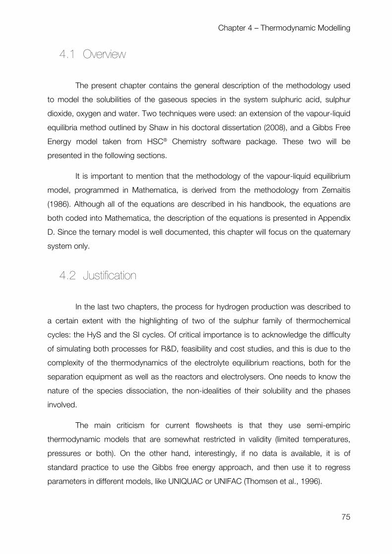
Chapter 4 – Thermodynamic Modelling

75

4.1 Overview

The present chapter contains the general description of the methodology used

to model the solubilities of the gaseous species in the system sulphuric acid, sulphur

dioxide, oxygen and water. Two techniques were used: an extension of the vapour-liquid

equilibria method outlined by Shaw in his doctoral dissertation (2008), and a Gibbs Free

Energy model taken from HSC® Chemistry software package. These two will be

presented in the following sections.

It is important to mention that the methodology of the vapour-liquid equilibrium

model, programmed in Mathematica, is derived from the methodology from Zemaitis

(1986). Although all of the equations are described in his handbook, the equations are

both coded into Mathematica, the description of the equations is presented in Appendix

D. Since the ternary model is well documented, this chapter will focus on the quaternary

system only.

4.2 Justification

In the last two chapters, the process for hydrogen production was described to

a certain extent with the highlighting of two of the sulphur family of thermochemical

cycles: the HyS and the SI cycles. Of critical importance is to acknowledge the difficulty

of simulating both processes for R&D, feasibility and cost studies, and this is due to the

complexity of the thermodynamics of the electrolyte equilibrium reactions, both for the

separation equipment as well as the reactors and electrolysers. One needs to know the

nature of the species dissociation, the non-idealities of their solubility and the phases

involved.

The main criticism for current flowsheets is that they use semi-empiric

thermodynamic models that are somewhat restricted in validity (limited temperatures,

pressures or both). On the other hand, interestingly, if no data is available, it is of

standard practice to use the Gibbs free energy approach, and then use it to regress

parameters in different models, like UNIQUAC or UNIFAC (Thomsen et al., 1996).


76

The model contained in this chapter, along with the model obtained from HSC

Chemistry, are a starting point towards rigorous thermodynamic modelling, that in the

future could be implemented for more components and modified to predict a broader

range of temperature and pressure conditions. This will then be compared with the

Gibbs Free Energy model, which is the standard non-experimental electrolyte modelling

technique. In the following section, some equilibrium chemistry considerations are

mentioned, in order to introduce the speciation that one has to become familiar with in

this work.

4.3 Sulphuric Acid Equilibrium

4.3.1 H2SO4 dissociation

According to the review performed by Zemaitis (1986), when pure liquid, the

electrical conductivity of sulphuric acid is very high, as well as its viscosity. In this state,

self-dissociation occurs, according to the following reaction:

32 4 4 42H SO H SO HSO

This has been proposed as the main cause for high conductivity. Simultaneously,

a second reaction has been suggested:

2 4 3 2 2 72H SO H O H S O

, where self-dissociation products have been estimated at 0.043 molal in total,

which is by no means a negligible amount. This needs to be compared with the total

proton and hydroxide ion presence in water, calculated as 2x10-7.

When in solution with water, the polyprotic acid dissociates into sulphite and bi-

sulphite, according to the following overall reaction:

22 4 4 42H SO H HSO H SO

While the first reaction is thought to be complete, or having a large reaction

constant; the second dissociation prevails in only low sulphuric acid concentrations. This

is critical, as low concentrations are relevant to the conditions involved current flowsheets


77

(Jeong, 2005, Brown et al., 2003). According to research performed by Young and Blatz

(1949), the chemical equilibrium diagram between species and concentration of sulphuric

acid in solution is shown in Figure 1. The data was taken from 0.06 to 2.34 moles of

water per mole of sulphuric acid, a non-standard method of measuring, but revealing

experimentally that concentrated sulphuric acid leads to rare species such as H5SO5+.

However, the equation

2 4 2 5 5 4H SO H O H SO HSO

is very rare for concentrations lower than 50%, and were not included in the model. A

review done in this work confirmed that the salting out effects for higher concentration

acid solutions of sulphuric acid are scarce, or not at all to be found in literature. In his

experiments, a 1040 cm-1 band was seen by Young and Walrafen (1961) that we could

confirm experimentally for higher concentrations in our Raman setup, discussed in

Chapter 5.

Figure 1. Equilibrium of concentrated aqueous H2SO4 at 25 °C.

Interestingly, these measurements were performed using dispersive Raman

spectroscopy, an advanced technique at the time.


78

As pointed out by Zemaitis, the second dissociation constant has been the

subject of much study. In this work, the reaction rate was taken as the Gibbs Free

energy polynomial function fitted to between 20 to 80 degrees °C. These are shown

below, fitted to the simplest equation possible for ease of calculation.

Figure 2. Sulphite formation from SO2 dissociation equilibrium constant, from 25 to 80 °C.

Figure 3. Water dissociation equilibrium constant, from 25 to 80 °C.

y = 3E‐06x2 ‐ 0.0006x + 0.0292

0.00E+00

2.00E‐03

4.00E‐03

6.00E‐03

8.00E‐03

1.00E‐02

1.20E‐02

1.40E‐02

1.60E‐02

1.80E‐02

25 35 45 55 65 75

Reaction Rate Constant

Temperature °C

Aqueous Sulphite Dissociation

y = 9E‐17x2 ‐ 5E‐15x + 9E‐14

0.00E+00

5.00E‐14

1.00E‐13

1.50E‐13

2.00E‐13

2.50E‐13

3.00E‐13

25 35 45 55 65 75


Temperature, °C

Water dissociation


79

Figure 4. Aqueous Bisulphite formation, from sulphite. 25 to 80 °C.

Figure 5. Sulphuric acid ionization, or sulphate formation, 25 to 80 °C.

y = 3E‐12x2 ‐ 1E‐09x + 9E‐08

0.00E+00

1.00E‐08

2.00E‐08

3.00E‐08

4.00E‐08

5.00E‐08

6.00E‐08

7.00E‐08

25 35 45 55 65 75


Temperature, °C

Aqueous Bisulphite Formation

y = 3E+12e‐0.089x

0.00E+00

5.00E+10

1.00E+11

1.50E+11

2.00E+11

2.50E+11

3.00E+11

3.50E+11

25 35 45 55 65 75 85


Temperature, °C

Aqueous Sulphate Formation


80

Figure 6. Bisulphate formation, from initial sulphuric acid dissociation. 25 to 80 °C.

Figure 7. Acid recombination (from sulphur trioxide). 25 to 80 °C.

y = 2E‐06x2 ‐ 0.0004x + 0.0183

0.00E+00

2.00E‐03

4.00E‐03

6.00E‐03

8.00E‐03

1.00E‐02

1.20E‐02

0 10 20 30 40 50 60 70 80 90


Temperature, °C

Aqueous Bisulphate Formation

y = 9E‐15e0.1245x

0.00E+00

2.00E‐11

4.00E‐11

6.00E‐11

8.00E‐11

1.00E‐10

1.20E‐10

1.40E‐10

1.60E‐10

1.80E‐10

2.00E‐10

0 10 20 30 40 50 60 70 80 90


Temperature, °C

Aqueous Acid Formation from SO3


81

Figure 8. Gaseous acid dissociation to SO3 in the gas phase, 25 to 80 °C.

Once the reaction rates were developed, and analysed, stating that none of

them had negligible effects onto the model, one could then plug in the respective

equations into Shaw’s model to include H2SO4. It is evident that no solid reactions were

considered, nor formation of a 2nd liquid phase.

y = 3E‐11e0.1112x

0.00E+00

5.00E‐08

1.00E‐07

1.50E‐07

2.00E‐07

2.50E‐07

0 10 20 30 40 50 60 70 80 90


Temperature, °C

Gaseous Acid Dissociation


82

4.4 Problem Set Up

The following is the schematic representation of the problem:

Figure 9. Problem Set up (quaternary).

The aqueous solution containing sulphuric acid consists of the following

chemical equilibrium reactions:

Sulphuric acid first dissociation or sulphate formation

Bisulphate formation

Water dissociation

Sulphur dioxide dissociation or sulphite formation

Bisulphite formation


83

4.4.1 Reaction Equations

The following equations are used in the VLE calculations, each equation

represents a distinctive reaction, either gaseous or liquid.

Table 1. Reactions involved and corresponding chemical equations.

Reaction Equation

Sulphur dioxide dissociation (leading to Bisulphite) 2

3

2

[ ][ ]

[ ]SO

HSO HK

SO

Water dissociation [ ][ ]waterK H OH

Sulphite dissociation (leading to Sulphite) 3

23

3

[ ][ ]

[ ]HSO

SO HK

HSO

Acid dissociation (leading to Bisulphate) 2 4

4

2 4

[ ][ ]

[ ]H SO

HSO HK

H SO

Sulphate dissociation (Leading to Sulphate) 4

24

4

[ ][ ]

[ ]HSO

SO HK

HSO

Liquid Acid formation from Sulphur Trioxide(aq) 3( )

2 4( )

3( ) 2

[ ]

[ ][ ]aq

aqSO

aq

H SOK

SO H O

Gas Acid formation from Gaseous H2SO4(g) 2 4( )

3( ) 2 ( )

2 4( )

[ ][ ]

[ ]g

g gH SO

g

SO H OK

H SO

The useful form coded into Mathematica is in the form:

c d

C C D DT a b

A A B B

m mK

m m

Next, the equilibrium equations will be presented.


84

4.5 Equilibrium equations

In this section, equations from the literature are taken and adapted from the

Henry’s Ensemble Law, modified via the Zemaitis (1986) methodology, and incorporated

to Mathematica, they also represent the dissociation as a function of ionic molarities and

activity coefficients for all species. Along with the electroneutrality condition, material

balances and fugacity and activity coefficients, the thermodynamic modelling is fully

posed.

4.5.1 Vapour-liquid Equilibrium Equations

The following equations are the ensemble equations relevant to the gas-liquid

exchange for the species in question.

Vapour-liquid equilibria of oxygen

2

2 2 2 2 2

, ( )exp

sO w w

O O O O O

v P Py P H m

RT

Vapour-liquid equilibria of sulphur dioxide

2

2 2 2 2 2

, ( )exp

sSO w w

SO H O SO SO SO

v P Py P H m

RT

Vapour-liquid equilibria of sulphuric acid

2 4

2 4 2 4 2 4 2 4 2 4

, ( )exp

sH SO w w

H SO H SO H SO H SO H SO

v P Py P H m

RT

Vapour-liquid equilibria of water

2 2 2

( )exp

ss w w

H O H O H O w w

v P Py P a P

RT


85

4.5.2 Reaction Equations

These following equations are taken from the identities drawn upon on Chapter

3. They are the equilibrium reaction constants as a function of molar concentration and

activities (for the liquid phase).

Water dissociation

- -

2

H H OH OHH O

w

m mK

a

Sulphur dioxide dissociation

- -3 3

2

2 2( ) ( )

H H HSO HSOSO

wSO aq SO aq

m mK

m a

Bisulphite formation

2- 2-3 3

-3

- -3 3( )

H H SO SO

HSOHSO aq HSO

m mK

m

Sulphuric acid dissociation

- -4 4

2 4

2 4 2 4( ) ( )

H H HSO HSOH SO

H SO aq H SO aq w

m mK

m a

Bisulphate formation

2- 2-4 4

-4

- -4 4( )

H H SO SO

HSOHSO aq HSO

m mK

m

The rest of the reactions were implemented as a numerical approximation of the

HSC thermochemical database, in order to increase the speed of convergence. It has to


86

be noted that an accurate first guess is imperative if one is to achieve convergence

quickly, or to achieve it at all.

4.5.3 Fugacity Coefficients

For the gaseous phase, the molar volume of the mixture and the fugacity

coefficients were required. The equation of Nakamura was used, which is a perturbed

harp-sphere model used in Shaw’s doctoral thesis (2008) and originally published by

Nakamura et al. (1976). This equation makes it possible to determine volumetric

properties of gases with different polarities, although approximations on the published

parameters were needed as they were not readily available for oxygen, SO3 and H2SO4.

The equation of interest is the following:

2 3

3

1

(1 ) ( )

RT aP

V v v c

Where

4

b

v

The full method is a semi-empirical way to determine volumetric properties taken

from experimental data, and is described elsewhere (Shaw, 2008).

4.5.4 Activity Coefficients

The method of Pitzer (1973), which is a generalized correlation method to

calculate activity coefficients depending on the nature of individual electrolytes was used.

The method is essentially a sum of the different ion-ion, ion-molecule and molecule-

molecule interactions for each species, totalling a repulsive or attractive force that will

dictate the solvation behaviour of the mixture.


87

4.5.5 Selection of Fugacity and Activity Coefficients Methods

Previous to the work of Pitzer and Kim regarding the activity and osmotic

coefficients for mixed electrolytes (1974), there was no simple or accurate description of

multi-component electrolyte solution behaviour. Their work demonstrates a semi-

empirical method to determine solubility behaviour spanning different ionic strengths and

chemical compositions over a wide range of single components. These equations were

tested for 69 sets of mixtures showing on average a deviation of less than 0.01 in 36

cases and above 0.05 in only seven cases, all involving OH1- and Cs+. Since in this work,

the ability to combine solubility properties of such distinct electrolytes (H2SO4 and SO2)

was paramount, it was deemed acceptable to continue using the Pitzer model for the

prediction of VLE behaviour.

With respect to the fugacity coefficient, and continuing the criteria selected by

Shaw in his doctoral dissertation, it was considered prudent to remain using the

Nakamura equation of state for gaseous calculations, as this presented reasonable

approximations to the experimental data. This was also selected for simplicity and ease

of modification, since it’s a simple, perturbed hard-sphere equation, originally presented

for carbon dioxide, but suitable for SO2 molecules.

4.6 Summary of Code Changes

This is an overview of the code changes that are included in the ternary vapour-

liquid equilibrium model. It is a modified version stemmed from the version submitted in

Shaw’s doctoral thesis and the results published in the IJHE paper in 2010, and used in

the ternary models in this project. These are intended to be merely descriptive, all the

code is included in Appendix D. The main modifications had to do with the following

aspects:

‐ Estimation of molecular interaction parameters ‐ Guessing of initial values ‐ Mathematical method to solve the system of algebraic equations ‐ Iterative procedure to improve accuracy of partial pressures ‐ Fitting of reaction rate constants


88

These modifications were included in the quaternary system. The reaction rate

constant fitted curves are explained in section 4.3.1.

4.6.1 Molecular Interaction Parameters

As stated in the introductory part of this thesis, one of the justifications of this

work was to establish the solubility behaviour of sulphur dioxide in aqueous sulphuric

acid solutions at moderate temperatures and pressures. The difficulty of pursuing this

objective is clearly noticeable by the almost non-existent body of experimental work with

this particular set of components.

Apart from the obvious modern approach of molecular simulation, one of the

main solutions to this is to approximate values of interaction to similar components,

hence acquiring a certain similarity of results in comparison to the original mixture. For

example, gathering interaction parameters from a volatile electrolyte vapour liquid

equilibrium dataset would be a starting point for a sulphur dioxide mixture in water. This

is what it was done in this project, but instead, using the existing parameters of

interaction between CO2 (a mild volatile electrolyte, although less soluble in water than

SO2) and water. If deemed reasonable, molecular weight was used instead for sulphuric

acid.

4.6.2 Guessing of initial values

Promotion of convergence in chemical engineering calculations is a daily

problem in research. This problem was also noticed in the algorithms used to calculate

vapour liquid equilibria in this project. Originally, the ternary code used the Newton’s

method of solving simultaneous algebraic equations. This was superseded by the Secant

method in the quaternary calculations, as it limits the number of a certain variable with

the selection of a maximum and a minimum. The other values are then constrained so

that the overall calculation takes less computing power, as well as an arithmetically

sound result. This was needed as the activity coefficient calculations (and several other

variables) acquired a complex number value as the iterations progressed. This optimized

the calculations significantly.


89

4.6.3 Secant Method

A computational procedure described by Wolfe (1959) for the solution of not

necessarily linear equations is incorporated in Mathematica software, in which the only

hard theoretical assumption is that the solution function has a second derivative, and

consists, in short, in the iteration of a step in which there are n trials at hand, where the

solutions are replaced between two values (the aforementioned maximum and

minimum).

In this work, since the activity coefficient values can only be between 0 and 1 (in a

thermodynamically consistent model), it was deemed reasonable to limit these values

between -1 and 2, which gave plenty of range to acquire reasonable approximations for

other variables. In case a coefficient went slightly below 0, or more than one, which is

very common in complex multiphase vapour liquid equilibria calculations, there was

enough tolerance for values several iterations previous to the final solution.

4.6.4 Iterative behaviour of VLE model

The methodology outlined by Zemaitis suggested the construction of a equation-

based vapour liquid equilibrium model starting from the binary reactions of SO2-H2O and

increase its complexity by adding subsequently O2 and then H2SO4. As the complexity

progressed, the flexibility of the code was reduced, and the initial value “elasticity” was

compromised. This affected the accuracy of the vapour pressure guesses of each

species, that were directly connected to fugacity calculations. This limitation was solved

by looping the entire code in order to achieve an enhanced guess and then proceed with

the calculations. This approach reduced the amount of iterations needed for

convergence and reduced the amount of complex numbers showing up in the console,

by merely doubling the lines of code in the program.


90

4.6.5 Reaction Rate Constants

Finally, the HSC Chemistry software was used to determine an algebraic

expression for reaction rate constants for the different equilibrium reactions taking place,

either in the gaseous form or the liquid form. For ease of use, the expressions were then

formulated between the temperature ranges of use (20 and 80 degrees) and then were

coded into the quaternary model (see section 4.3) These in turn were only used in that

particular range, guaranteeing the validity of the values selected in this work.

4.6.6 Electroneutrality

Finally, the condition referred to as “electroneutrality” has to be set, and this just

means that the electric forces between ions are so strong that theoretically, they instantly

neutralize each other’s fields, so as to have an overall electric charge of ~ 0. This can be

expressed as:

2 23 4 3 4

2[ ]H OH HSO HSO SO SO

m m m m m m

In essence, the important VLE equilibrium equations have been presented in

these sections. These equations, along with their supporting derivations and

implementations are entirely presented in code form in Appendix D. This Mathematica

model is then compared with the HSC calculations, as well as presented in more detail

with a sample calculation, tabulating results as needed.

4.7 Sample Calculations: HSC and Mathematica

Figure 10 shows the calculation of a ternary system at constant temperature,

while changing pressures. This data is either tabulated raw in spreadsheet format, or

displayed as a diagram with axis and different colors for each species involved in the

calculation. This was considered the easiest way to visualise the results, but in order to

compare components on an individual basis, tabulated data was converted to multi-

curve plots, where each curve represented a single run of one species.


91

Figure 10. Sample Calculation of ternary system, 40 degrees, 0-5 bar.

In the calculation shown in Figure 10, one can appreciate the decrease of

concentration of sulphur dioxide gas as the total pressure of the system increases. One

expects then that the solubility of SO2 increases, and this is confirmed by the rise of the

red curve labelled as SO2(a) in the bottom of the graph. It is natural to see that although

the concentration of gases in the liquid phase is relatively low in comparison to the

gaseous state, it is by no means negligible. This type of visualization is helpful to see the

relation held between the gaseous concentrations and the ionic concentrations of the

dissociation products.


92

Figure 11. Excel format, from raw tabulated data shown in Appendix C.

In the calculation shown in Figure 11, a more detailed analysis can be performed

via either decreasing the scale of the concentration on the y-axis, or one can filter the

species involved as to see which ones are the main players in that particular calculation.

Evidently, these dissolved amounts will be directly related to the system input in the HSC

start spreadsheet. When very little amounts of ions were present, one had to recur to

logarithmic scales, or reducing the pressure range in order to visualize and compare

between ions.

Table 2. Activity coefficients of quaternary species vs. temperature, from 25 to 80 °C.

80% of the time of each calculation is spent on the initial guesses. It is extremely

important to be familiar with the quantities that are involved in each experiment, since an

order or magnitude difference can mean divergence of the calculation and in those

situations, restarting of the kernel is unavoidable.


93

4.8 Discussion

Solubility of SO2 in water is a subject of many studies in the last century. The

publication of Hales (1973) is a fine example of an experimental study of SO2 solubility for

atmospheric purposes, and the author compares it with this work due to the similarities

of questions that arose during their experiments and after their work was summarized

along with their advantages and disadvantages when making the theoretical

considerations included in the publication. A key finding of Hales is the fact that the

authors reported an increasing source of error as the concentration of SO2 decreased in

the experiments, acquired via a flow technique, different from the static technique that

it’s developed in this work and described in Chapters 5 and 6. In this case, the

theoretical assumption that the second dissociation did not take place leads them to

inconsistencies in their experimental data, which was a source of undesirable

discrepancy between experiments.

In this work, and taken from the lessons learned by Hales, there was no single

possible reaction that was neglected in the system, including those involving sulphur

trioxide. This is a key strength of the Mathematica model, along with the fact that the

Mathematica model is the only rigorous equation-based attempt at Vapour Liquid

equilibrium, that can be extended for more species and has a strong theoretical

foundation with the Pitzer interaction model, the Nakamura equation of state and the

ensemble Henry’s Law in the form presented by Zemaitis (1986).

Also, the calculations are comparable with the Gibbs free energy model, a well-

known industry based method to determine non-ideal behaviour in electrolyte solutions,

with a semi-empiric support taken from thermochemical measurements.

Deviations and uncertainties of the calculations developed in this chapter cannot

be discussed without the comparison with experimental data (Chapter 6), although it is

likely that the lack of a large enough body of data required to regress the interaction

parameters needed for the activity coefficient calculations could be a source of instability.

Without a sufficient body of experimental data, it is impossible to regress the model

adequately enough to be certain that the solubility predictions are within at least 5% of


94

the true values, considering the uncertainties shown in the experimental section of this

work, in Chapter 6.

It is very likely that the prediction at higher pressures is just more than the

approximate binary interaction parameters due to the lack of experimental data. One

could suggest that there could be other sources of error:

Neglect of the clathrate hydrate formation in the model, experimentally

evidenced when taking small samples from the equilibrium apparatus.

This would mark the need for a SVL equilibrium model, with deposited

solids that would change entirely the volume calculation equations.

Wrong prediction of speciation (unknown species are present)

Formation of complexes, and even elemental sulphur.

Although there are limitations to the not very flexible set of equations in the

Mathematica model, it is a very good starting point to aid in the planning of experimental

data that is necessary for the conditions relevant to the acid decomposition in both the SI

and the HyS cycles.

4.9 Summary

A working set of equations has been devised to represent the vapour-liquid

equilibria of multicomponent aqueous solutions, containing sulphuric acid, oxygen and

sulphur dioxide; including the formation of sulphur trioxide simultaneously as a

dissociated product of the sulphuric acid gaseous dissociation and as a reagent to form

acid once dissolved in water.

The thermodynamic treatment together with liquid phase reactions, material

balances and the condition of electroneutrality can be used to devise a set of equations

so that for known input amounts of species (sulphur dioxide-H2SO4-water) and starting

conditions the resulting equilibrium is modelled. For a solute and solvent pair there will

be x independent equations in x unknowns, which when solved will give the amount of

gas that dissolves, associated molalities of all species in the liquid phase, mole fractions

in the vapour phase and a vapour production rate.


95

While there are many ways to calculate the fugacity and the activity of the

aforementioned mixture, it was decided to continue the methodology described by

Zemaitis, using the parameters determined by Shaw in his doctoral thesis, containing the

most applicable calculations for SO2 and sulphuric acid. Beutier and Renon’s (1978)

model for the activity coefficient was developed as an extension to the work by Edwards

(1975, 1978) and specifically considered sulphur dioxide/water equilibria, amongst other

mixtures, for sour water strippers. The Nakamura (1976) method used to predict

fugacity coefficients comes from work on prediction of thermodynamic properties of gas

mixtures containing polar and non-polar molecules.

This is further supported by the calculation of the same equilibrium using HSC

Chemistry, a software package that uses the Gibbs Free Energy minimisation technique

to provide a glance at the vapour liquid equilibrium and speciation in the aforementioned

system.

It is worth remembering that H2SO4, SO2 and water are polar molecules and this

work’s rigorous model is intended to be a good approximation for a broad range of

conditions, relevant to electrolyte modelling in thermochemical cycles. In the next

chapter, the experimental activities of this project will be presented, along with the

considerations that were deducted from both models.


BEUTIER, D. & RENON, H. 1978. Representation of ammonia-hydrogen sulfide-water, ammonia-carbon dioxide-water and ammonia-sulfur dioxide-water vapor-liquid equilibriums. Industrial & Engineering Chemistry Process Design and Development, 17, 220-30.

BROWN, L. C., BESENBRUCH, G., LENTSCH, R., SCHULTZ, K. R., FUNK, J. E. & ATOMICS, G. 2003. Alternative flowsheets for the sulfur-iodine thermochemical hydrogen cycle, United States. Department of Energy. Oakland Operations Office.

EDWARDS, T. J., MAURER, G., NEWMAN, J. & PRAUSNITZ, J. M. 1978. Vapor-liquid equilibria in multicomponent aqueous solutions of volatile weak electrolytes. AIChE Journal, 24, 966-976.

EDWARDS, T. J., NEWMAN, J. & PRAUSNITZ, J. M. 1975. Thermodynamics of aqueous solutions containing volatile weak electrolytes. AIChE Journal, 21, 248-59.

HALES, J. M. & SLITTER, S. L. 1973. Solubility of sulfur dioxide in water at low concentrations. Atmospheric Environment (1967), 7, 997-1001.



PITZER, K. S. 1973. Thermodynamics of electrolytes. I. Theoretical basis and general equations. The Journal of Physical Chemistry, 77, 268-277.

PITZER, K. S. & KIM, J. J. 1974. Thermodynamics of electrolytes. IV. Activity and osmotic coefficients for mixed electrolytes. Journal of the American Chemical Society, 96, 5701-5707.



97


WOLFE, P. 1959. The Secant method for simultaneous nonlinear equations. Commun. ACM, 2, 12-13.

YOUNG, T. & WALRAFEN, G. 1961. Raman spectra of concentrated aqueous solutions of sulphuric acid. Transactions of the Faraday Society, 57, 34-39.

YOUNG, T. F. & BLATZ, L. A. 1949. The variation of the properties of electrolytic solutions with degrees of dissociation. Chemical Reviews (Washington, DC, United States), 44, 93-115.

ZEMAITIS, J. F., CLARK, D. M., RAFAL, M. & SCRIVNER, N. C. 1986a. Activity Coefficients of Strongly Complexing Compounds. Handbook of Aqueous Electrolyte Thermodynamics. John Wiley & Sons, Inc.

ZEMAITIS, J. F. J., CLARK, D. M., RAFAL, M. & SCRIVNER, N. D. 1986b. Handbook of aqueous electrolyte thermodynamics.

99

Chapter 5

Experimental Design

100

Chapter 5 Table of Contents Background ........................................................................................................................... 105

5.1 Overview .............................................................................................................................. 105

5.2 Aim ...................................................................................................................................... 105

5.3 Previous Equilibrium Still Designs ......................................................................................... 106

5.3.1 Mark I and Mark II ............................................................................................................... 108 5.3.1 Mark III ................................................................................................................................ 110 5.3.2 Experimental Procedure ...................................................................................................... 115 5.3.3 Spatial Thermal Uniformity ................................................................................................... 116 5.3.4 PID Damping ....................................................................................................................... 117 5.3.5 Sample Flashing .................................................................................................................. 118

5.4 Requirements: Visualisation, Solids and Phase determination .............................................. 120

5.4.1 Flow visualisation ................................................................................................................ 120 5.4.2 Solid Formation: SO

2 Clathrate Hydrate ................................................................................ 121

5.4.3 Aqueous and SO2 phase determination ................................................................................ 122

5.5 Thermal-switch Incident ....................................................................................................... 123

5.5.1 Root Cause Analysis ........................................................................................................... 123 5.5.2 Mark III Follow-up ................................................................................................................ 124

Mark IV Design ..................................................................................................................... 126

5.6 Aim ...................................................................................................................................... 126

5.7 Material Considerations ........................................................................................................ 126

5.8 Pressure Vessel Calculations................................................................................................ 127

5.8.1 Operating Pressure ............................................................................................................. 128 5.8.2 Allowable Stress .................................................................................................................. 128

5.9 Thermal Properties ............................................................................................................... 129

5.9.1 Preliminary thermal calculations ........................................................................................... 129 5.9.2 Problem set-up ................................................................................................................... 130 5.9.3 Lumped System Analysis for transient heat conduction Rig Design ...................................... 130

5.10 Equipment & Instrumental Design ........................................................................................ 132

5.11 Spectroscopic theoretical background ................................................................................. 133

5.11.1 Infrared spectroscopy ......................................................................................................... 133 5.11.2 Raman spectroscopy .......................................................................................................... 134 5.11.3 Raman Spectrometer .......................................................................................................... 134 5.11.4 FTIR Spectrometer .............................................................................................................. 139 5.11.5 Auto Titrator ........................................................................................................................ 141

5.12 Infrared Materials .................................................................................................................. 141

5.12.1 Silicon ................................................................................................................................. 141 5.12.2 Germanium ......................................................................................................................... 144 5.12.3 Zinc Selenide ...................................................................................................................... 145

Chapter 5: Experimental Design

101

5.13 Chemical Inertness ............................................................................................................... 146

5.14 Infrared Developments ......................................................................................................... 147

5.14.1 Gas Cell .............................................................................................................................. 147 5.14.2 Full ATR Configuration Results ............................................................................................ 150 5.14.3 Liquid Cell ........................................................................................................................... 152

5.15 Mark IV Additional Considerations ........................................................................................ 153

5.15.1 Weight and Dead Volume .................................................................................................... 153 5.15.2 Germanium ATR Design ...................................................................................................... 154 5.15.3 Thermal Uniformity .............................................................................................................. 157

5.16 Summary ............................................................................................................................. 159

References for Chapter 5 ...................................................................................................... 160

102

List of Figures

Figure 1. Original still by Othmer (1952), p.1865. Still body, 19” long. .................................... 107

Figure 2. Simplified Schematic diagram of Mark I to III. (Shaw, 2008) .................................... 108

Figure 3. Fluoropolymer coating used in Mark II, taken from Shaw’s thesis (2008). ............... 110

Figure 4. Mark II. T: Thermocouple gland. P: Pressure transducer. V1: Gas Valve. V2:

Liquid Valve. E: pH probe. V8: Liquid Sampling valve. V9: Gas sampling valve. ..................... 111

Figure 5. Mark III in operation, with rotating still and insulation in display. .............................. 112

Figure 6. Mark III Mechanical detail. Distances in mm. ........................................................... 113

Figure 7. Mark III run at 60 °C. .............................................................................................. 115

Figure 8. Surface vs. Well thermal measurements, Mark III rig. .............................................. 117

Figure 9. Example of non-dampening of controller signals: “spiking” temperatures. .............. 118

Figure 10. Iodometry analysis in a pressurized aqueous SO2 solution. ................................... 119

Figure 11. Van Berkum’s (1979) optical autoclave, with measurement instruments . ............. 121

Figure 12. Principle of operation of in-situ vibrational spectrometry. ...................................... 133

Figure 13. Preliminary Raman Experiments pointing at certain operating aspects of

acquisition. Acetonitrile acquired without caps. Light contamination with Microscope

objective. SO2 exposure, with correlation to light contamination peaks. ................................. 137

Figure 14. Raman PEEK Probe designed by the author. ....................................................... 139

Figure 15. Varian 660 Spectrometer, showing the optical path of the IR source and

internal components. ............................................................................................................ 140

Figure 16. Optical IR Transmission Curves for Silicon, Germanium and ZnSe. (Crystran,

2012) .................................................................................................................................... 143

Figure 17. Transmission model T%(n,r,t) for Germanium, coded in Mathematica. ................... 144

Figure 18. First design attempt at a gaseous cell. ................................................................. 148

Figure 19. CAD designed cell, using Inventor™..................................................................... 148

Figure 20. Final Gas Cell Version (Spectroscopic High-Accuracy Gas Cell – SHAG Cell). ...... 149

Figure 21. Interferogram of the in-house gas cell, with ZnSe windows. ................................. 150


103

Figure 22. ATR configuration with highlighted IR emission path. ............................................ 151

Figure 23. Germanium ATR Configuration with fibre optics and no sample............................ 151

Figure 24. Maximum compressive stress inside the liquid PTFE liner, within the liquid cell. .... 153

Figure 25. Mark IV rig body, including major sections. ........................................................... 154

Figure 26. Final ATR configuration, Top and Side view of assembly. ..................................... 156

Figure 27. FLIR Imaging of the rig within the water bath a) outside the water bath and b)

submerged. Acknowledgments to Dennis Cumming. ............................................................ 157

Figure 28. A) Ge Prism configuration, top lid with recess and locating pins. ......................... 158


104

List of Tables

Table 1. Volumes of top, bottom and connecting sections of Mark-II .................................... 109

Table 2. Description of experimental apparatuses used for the acquisition of sulphur

dioxide, oxygen, water and sulphuric acid vapour liquid equilibria. ........................................ 114

Table 3. Thermal and Mechanical Properties of commercial GF-PTFE. (Quadrant, 2011) ...... 127

105

Background

5.1 Overview

In this Chapter, the research leading to the design of the final equilibrium

apparatus is described. Picking up from Shaw’s research and funded by the

HyCycleS project, it continued to be funded through the final stage of the EU FP7

final deliverable, as well as being funded partly by the Mexican Government. The

author continued the experimental work and pursued the incorporation of

sulphuric acid into the project, using novel technologies and one of a kind in-situ

setup.

The chapter starts with the aim of the design, as well as the background

of the former generation of rigs, discussing shortcomings, possible solutions,

making a case for the analysis of the instrumental additions to the apparatus and

finally, some findings prior to the operation of the final version of the equilibrium

still, the Mark IV.

5.2 Aim

Experimental work in this project consisted on gathering vapour-liquid

equilibrium data. This was initially done with Shaw’s designed stills, Mark I to III,

but some shortcomings were identified, that led to the development of a new rig.

The idea behind the new setup was to tackle inconsistencies in the equilibrium

measurements, specifically the chemical analysis and the uncertainty of the

results, which had to do with two questions:

How to minimise experimental uncertainties, inherent to the

equilibrium still measurements.

What is the nature of the ionic speciation that could not be

determined with analytical techniques featured in previous rigs.


106

These questions had to be addressed, so a considerable amount of time

in this project was allocated to the design of a reactor that could avoid the

shortcomings that were identified with the former generation of VLE still.

Analysis of the data acquired with previous rig designs (Mark I to Mark III)

led to important findings, including the necessity of refocusing the chemical

analysis approach to equilibrium measurements (in-situ). A detailed step-by-step

description of the engineering that took place to produce the Mark-IV rig is

presented in this chapter, along with the associated calculations and technical

necessary in the process.

The objective of the experiments is to successfully bring into contact the

species of interest (ternary: SO2, O2 and H2O – quaternary: including H2SO4).

Select quantities of each species would be inserted into the equilibrium apparatus

in question, mixed and then analysed, providing a full picture of the

thermodynamic status of the system. The rig needs to withstand temperatures of

up to the boiling point of the solution, be resistant to acid corrosion and be able to

withstand 20 bar of hydraulic static pressure. Ideally, one would sample the

species without disturbing the equilibrium.

5.3 Previous Equilibrium Still Designs

Prior to this research project, several VLE stills were designed and are

presented in Shaw’s doctoral thesis (2008). The principle via which the rigs

operated was based on the still developed by Othmer (1952), and was

constructed in-house. The original Othmer still is shown in Figure 1. In the figure,

several elements are shown: T1-T5 thermocouples, a) cartridge Heater wells, b)

liquid sample outlet, c) peep sights, d) cone shape top plate for condensate, e)

vapour outlet pipe, f) vent valve for noncondensable gases, g) inlet tube for

condensate return. The original equilibrium design in this work was inspired by this

first static still. A brief description of the apparatuses leading to the Mark-IV is

discussed in the following sections, inspired by the first Othmer still.


107

Figure 1. Original still by Othmer (1952), p.1865. Still body, 19” long.


108

5.3.1 Mark I and Mark II

The first reactor, Mark I, is shown schematically in Figure 2. It had a

volume of 1005.8 cm3 and it was made partly from stainless steel, where

sometimes QVF® glass chambers were attached for low pressure experiments.

The chambers were united via a pipe and were isolated using Swagelok valves.

The outside diameter of the chambers was 140 mm and the inner diameter was

100 mm, which narrowed down to a cone with an angle of 30°, to a minimum

through diameter pipe of 30 mm. The length of the apparatus was 800 mm in

total, and reached a mass above 10 kg. The pipe connecting the chambers was a

¾” SS pipe that allowed liquids to move freely. The inter-valve section allowed for

the expansion of the liquid volume after complete gas dissolution.

Figure 2. Simplified Schematic diagram of Mark I to III. (Shaw, 2008)


109

Table 1. Volumes of top, bottom and connecting sections of Mark-II

Part Volume (in cm3)

Gas chamber (Top) 630.9 cm3

Liquid Chamber (Bottom) 302.7 cm3

Connecting Pipe Section 72.2 cm3

The Mark I design intensified the aqueous sulphur dioxide oxidation as the

stainless steel valves provided considerable wetted surface. This was further

identified by noting a decrease in operating pressure without apparent leakage.

The next iteration of the design included a fluoropolymer (DuPont® B5513-Green)

coating to limit the oxidation. Shaw (2008) describes the difference between the

Mark I and Mark II designs:

“All valves were stainless steel ball valves cleaned

to be compatible with pure oxygen. The pressure

transducer was a Sensortechnics CTE9035AY7 which

had a stainless steel body and diaphragm. The

thermocouples were Teflon insulated K type sensors

with an outer diameter of 4 mm installed via bored

through Swagelok® 4 mm compression fittings. The pH

probe was an Omega® PHE-5433-10 electrode housed

in a Ryton® body having a Temperature Range of -5 to

135 °C and a pressure rating of 500 psig at 25 °C. The

electrode had a triple junction reference cell of

KCl/AgCl, 3M KCl and a reference junction of Porous

PTFE. The electrode was installed through a 25 mm

port gland compression fitting. The apparatus was

hydraulically tested to a pressure of 60 bar with a

blanking plug in place of the pH electrode. The rig was


110

heated by a combination of 5 individually controlled mat, tape

and rope heaters attached to the outer surface. The control of

the rope heaters and data acquisition was the same for both

rigs…” (p.167)

The Mark I had no lining. A fluoropolymer coating was set to the Mark II

and is shown in Figure 3. Even though the lining was successful in reducing the

metal contact, the valve metal area that was interfacing with the liquid solution

nonetheless gave significant catalysis of the oxidation, although significantly less

than the original design. The wetted area is clearly shown relative to the coated

area in Figure 4. Note that, contrary to the original Othmer still, it is a rotating

apparatus and it skips the condenser section (compare with Figure 1).

Figure 3. Fluoropolymer coating used in Mark II, taken from Shaw’s thesis (2008).

5.3.1 Mark III

Following the oxidative problems in the Mark I and II, Shaw decided to

apply a full inert lining of the metal parts. This also needed to withstand the acidic

nature of the SO2 solutions that were part of the ternary research objective. The

logic behind this is explained in a paragraph of Shaw’s (2008) doctoral thesis:


111

“In addition to having low extractable content, fully fluorinated

fluoropolymers have very low surface energies, for example Teflon’s® lack

of polarity causes it to resist polar molecules such as water (Fleming et

al., 2001). The non-wetting property had the benefit that, during mixing,

water would not remain on the walls of the rig removing the likelihood of a

droplet of liquid remaining in the gas phase pot.” (p.170)

Figure 4. Mark II. T: Thermocouple gland. P: Pressure transducer. V1: Gas Valve. V2: Liquid Valve. E: pH probe. V8: Liquid Sampling valve. V9: Gas sampling valve.

While the metal extractable contents were selected as a critical priority for

the new design, the mechanical and thermal properties were omitted during the

Mark III design phase. This presented leakage problems throughout the


112

experimental phase of the Mark III, even though careful machining of the individual

components was ensured. This had important consequences in later stages of the

project, especially after the thermal switch incident. The mechanical and thermal

considerations for the new design will be discussed starting from section 5.9.

A picture of the Mark III in operation is shown in Figure 5, while a more detailed mechanical diagram of the Mark III design is shown in

Figure 6.

Figure 5. Mark III in operation, with rotating still and insulation in display.

The Mark III design was initially used in the first year of this project to

obtain thermodynamic data for binary and ternary mixtures. This data has been

published (Shaw et al., 2011), including a comparison with the literature and with

models pertaining preliminarily to SO2, O2 and water. A detailed discussion of the

results obtained with the Mark III rig is given in Chapter 6.


113

Figure 6. Mark III Mechanical detail. Distances in mm.

Table 2 contains a summary of the different rigs used in this project and

their main desired characteristics of the next generation of apparatus.


114

Table 2. Description of experimental apparatuses used for the acquisition of sulphur dioxide, oxygen, water and sulphuric acid vapour liquid equilibria.

Rig Iteration

Main Characteristics Length of Operation

Mark I

Metal body, stainless steel liquid and gas valves, QVF® borosilicate glass attachment for liquid phase, <400 cm3, <1000 cm3 volume. Wetted metal parts.

See Shaw’s doctoral thesis.

Mark II Stainless steel body with green PTFE coating, SS valves, 800 cm3 volume.

See Shaw’s doctoral thesis.

Mark III

SS body with virgin PTFE lining, PEEK oxygen valves and transducers, PFA gas and liquid valves, 4 mm virgin PTFE lining, PEEK oxygen valves and transducers, 800 cm3 total volume, 16 bar maximum operating pressure.

In this project, July-2009 to Feb-2011.

Mark IV

15% Glass-reinforced PTFE body with stainless steel modular threaded frame inserts, Raman probe, liquid IR transmission cell, liquid UV-Vis cell and gas IR cell attachments. Maximum hydraulic pressure 16 bar, maximum design temperature 220 °C. Negligible zero-volume.

Aug-2012 to date

The rig had to be operated at relatively dangerous pressures in

comparison to other routine experiments and the use of corrosive and very toxic

media at high temperatures (SO2 at 120 °C) has significant health and safety

implications. A risk assessment was made. Key safety points were addressed.

One of the measures taken to provide a reasonable safety margin for the

operating pressure, was to commission the rig made out of steel and PTFE lining.

A permissible strength of the stainless steel at the operating pressures of 20 bar

was met with a reasonable 10 mm thickness, according to simple pressure vessel

calculations. Finally, the decision was made to manufacture the apparatus with at


115

least a 4mm thick PTFE lining, and a full stainless steel body, machined out of a

>180mm diameter rod.

This measure led to the full apparatus to weigh more than 35 kilos, with

the rotating stand included. Several rope and mat heaters were purchased,

totalling a heating power of almost 2 kW. Even with this heating capacity, the time

taken for a mild increase of 20 °C could take hours. And due to the fluctuating

behaviour inherent to a PID algorithm, thermal equilibrium between phases was no

easy task. This is covered thoroughly in section 5.3.4. Overall, not only was it very

tedious to operate, but moving the entire rig and the electrical connections

required special logistic arrangements and led to reduced experimental uptime at

the end. This has to be improved, and section 5.5 is dedicated to the discussion

of these aspects.

5.3.2 Experimental Procedure

A typical operating graph is shown schematically in Figure 7.

Figure 7. Mark III run at 60 °C.


116

The experimental procedure is explained in the Appendix A. In summary,

the rig is subjected to vacuum, and the valves are closed to isolate the phases. It

is important to close the phases and leave an “inter-valve” space to allow for liquid

expansion after the volatile electrolytes are fully dissolved in the solution medium.

This has an additional advantage discussed in the sampling section of this

chapter.

Input of the water is straightforward and is based on calculation of the

mass difference between a water bottle before and after its attachment to the rig.

The difference is assumed to have transferred to the rig, ignoring little compressed

nitrogen bubbles. The mass amount of water compared to the mass of the

bubbles that could be seen stagnant in the flow system was at least a thousand

times less. However, the volume that the bubbles occupied was not negligible, so

an experimental volume calculation was necessary for the individual chambers, as

well as the total rig volume.

On the gas side, two approaches could be taken: adding a known

composition mixture of O2 and SO2, and using a smaller cylinder to measure the

mass difference before and after the addition to the rig. On the other hand, one

could attach the SO2 first, add a certain amount (mass would be then dependent

on the initial SO2 cylinder pressure), then attach a higher pressure O2 cylinder, then

take advantage of the higher driving force of the oxygen to diffuse to the rig and

calculate the mass added. These data would then be related to the calculations

via experimental values of solubility and composition, in each phase. A more

detailed procedure for the Mark III and Mark IV is given in the Appendix A.

5.3.3 Spatial Thermal Uniformity

To cope with large amounts of heat transfer, rope heaters were used to

increase temperature in incremental discrete steps, following a PID algorithm

optimised in LabVIEW. Typical behaviour is shown in Figure 8. Since the feedback

thermocouples were in the surface of the chambers, a moving average was taken


117

into account to modulate the wattage drawn into the heaters. Although the

temperature control was achieved easily on the outside, considerable time was

required to achieve the gas and liquid bulk temperatures.

Figure 8. Surface vs. Well thermal measurements, Mark III rig.

The practicality of the experimental procedure was undermined by the

amount of time that it took the rig to attain equilibrium, having sometimes to wait 4

hours for near-uniform heating in both chambers, for relatively moderate set

temperatures (40 – 80 °C).

5.3.4 PID Damping

An important optimisation was introduced to the heater controller, to

avoid excessive heat generation for the rope heaters. This had to do with damping

the proportional and integral constants that characterize the behaviour of the PID

algorithm, to avoid spiking. An example of the aforementioned “spiking” is shown

in Figure 9. In this example, a temperature almost reaching the 120 °C mark was

attained when the set temperature was 50 °C. This proved to be hazardous in

higher temperatures, ranging from 50 to 80 °C, since the peak was even higher,

sometimes reaching the 240 °C maximum from the heaters.

0 50 100 150 20015

20

25

30

35

40

45

50T

(°C

)

Time (min)


118

Figure 9. Example of non-dampening of controller signals: “spiking” temperatures.

5.3.5 Sample Flashing

An important aspect of the rig design concerns how representative was

the sample taken just after the equilibrium was reached. Although pressurized

samples taken from the reactor were relatively much smaller than the overall

system volume (~2 cm3 vs. ~640 cm3), one could not determine the physical state

of the sample (dissolved or mixed immiscible liquid). This problem was highlighted

by the observation of a decreasing trend in concentration, as measured by

Iodometry of the liquid samples. This is shown in one of the experimental titrimetric

analysis in Figure 10.

0.1 0.2 0.3 0.4 0.5 0.6 0.710

20

30

40

50

60

70

80

90

100

110

T (

°C)

Time (h)

Set Temperature Temp 4 cm. away Lab Temperature


119

Figure 10. Iodometry analysis in a pressurized aqueous SO2 solution.

In this example, the std. deviation is =0.191 and the 95% confidence

interval was 0.132, an average uncertainty of 6.5%. The overall trend for SO2 to

volatilise into the ambient atmosphere while in solution is well defined. This was a

constant source of error that crippled efforts to precisely to determine the VLE

behaviour of the mixture. This was a vulnerability in comparison with the Othmer

still: the lack of a compensating pressure system had a perceivable effect on the

results gathered atmospherically.

While it was possible to make modifications to the rig and alleviate certain

of these shortcomings, the decision to make a fourth-generation still was

hastened by an incident that eventually caused the decommissioning of the Mark

III, discussed in section 5.5.

1.8

1.9

2

2.1

2.2

2.3

2.4Molality Sulphur Dioxide (m

ol SIv/kg water))

Time (15 minute intervals)

Iodometry Concentration

Iodometry Concentration


120

5.4 Requirements: Visualisation, Solids and Phase

determination

5.4.1 Flow visualisation

In the literature, particularly the work by Battino (1966) and Maass &

Maass (1928), on which Shaw’s experiments were based, flow within the system

was easily seen as the apparatus that the authors were using was made out of

glassware and very simple mercury manometers. Although simple, this greatly

eased the pinpointing of important stages within the vapour-liquid equilibrium

context of the system, such as the bubble point, dew point and the identification

of impurities. In contrast, the Mark III was designed to withstand high pressures

while remaining safe to operate, and so there was no opportunity to easily include

a sightglass without incurring higher costs and custom machining not possible in

the workshop. This was also an approach taken by van Berkum (1979), on which

we based the Mark IV sight-glass upgrade, even if only a one-way sight-glass.

Although not critical, it was desirable to obtain visual confirmation of the behaviour

of the mixture within the system, without the penalty of flashing solutes, as

explained in section 5.3.5.


121

5.4.2 Solid Formation: SO2 Clathrate Hydrate

According to several authors (Harvey et al., 1964, Mohammadi and

Richon, 2010), the conditions necessary for the formation of a crystalline white

clathrate hydrate are readily attained with moderate pressures (<10 bar) and

temperatures (from 279.9 to 285 K). This was identified as a white watery powder

after the sampling of liquids once equilibrium was reached. This was problematic,

as the molar quantities that are contained in the SO2 clathrate crystals are by no

means negligible, and were identified to cause further deviation from real molarity

values during Iodometry.

It is important to note that the liquid and gas valves providing isolation

during sampling is an advantage because each phase does not interfere with the

other during sampling. This means that, while the pressure inevitably dropped

during liquid sampling (as the liquid sampling valve is opened), the gas in the

gaseous chamber remained at equilibrium conditions if the liquid and gaseous

chambers were isolated via a valve, as the state variables were not modified

(decreased pressure in one chamber, not the two). Once the valves were opened

though (and the chambers equalized), equilibrium shifted (towards a higher

Figure 11. Van Berkum’s (1979) optical autoclave, with measurement instruments .


122

flashing and lower pressure) and it wasn’t further considered representative of

what was inside the rig during the experiment (generally, lower pressure=less

solubility, as shown in the Chapter 4 models, for both SO2 and O2).

5.4.3 Aqueous and SO2 phase determination

The validity of the sample taken was not only determined by the possibility

of equilibrium shift due to the volume state variable being changed in the system,

but also by the physical orientation of the rotating still. In other words, flashing the

sample and the rig being vertical or horizontal. This becomes clear if one

considers that gravity and density play a key role in the equilibrium distribution of

the different hypothetical phases within the liquid chamber. If it is hypothesized

that there are two liquid phases within the chamber, depending on the horizontal

orientation of the L1-L2 interface normal to the sampling point, one could sample

either a mixture of different phases, or a representative sample of only one of

them, depending on their volume. One could not possibly tell as there was no

sight glass as experiments were carried out. In low pressure preliminary

spectroscopic experiments (described further in section 5.11.3), peaks pointing to

the formation of a second liquid phase increased the suspicion of a second liquid

SO2 phase.

This incident, along with the interest of a fellow researcher involved in

thermochemical cycles, Bob Buckingham, from GA, sparked the objective to

obtaining visual confirmation of a possible formation of elemental sulphur in these

experiments (Buckingham, 2011). The relevance of this hypothetical finding is out

of the scope of this project, but it is noteworthy that this possible reaction is

relevant to the sulphur-sulphur thermochemical cycle. However, it was impossible

to identify the common yellow flakes of elemental sulphur in-situ. This was another

motivation to go for in-situ measurements and a sight glass for the new reactor. In

total, prior to the thermal switch incident (see section 5.5), more than 50 binary

and ternary data points were acquired.


123

5.5 Thermal-switch Incident

On the 21st of February 2011, multicomponent experiment #52

concluded. Standard procedure after its conclusion was to prepare the rig for the

next day’s run. This included drying of the rig for 1 to 2 hours. The method of

drying involved a regulated heat supply from the rope heaters and a compressed

air current venting out to the fume cupboard. This had two objectives: to delete

traces of sulphur dioxide inside the gas chamber and to dry the rig. Heating

remained controlled, as it limited excessive temperature drops due to evaporative

cooling from droplet remains inside the rig in contact with the compressed air. An

operating system crash occurred within the PC and, as there was no

implementation of software safe-mode, all five solid state relays in the data

acquisition module turned completely on, leading to the rope heaters to reach

their maximum temperature, only limited via the thermal switches, set at 240 °C.

After three hours, a quick click in the fuse box of the heater controller was noticed

and the system was shut down. The PTFE lining melted and was deemed

unusable. A root-cause analysis was then performed to determine the causes of

the incident.

5.5.1 Root Cause Analysis

A thorough inspection of the rig was performed after the incident. After

careful consideration, the conclusion that an electrical failure in the heater/relay

subsystem was the main cause of the malfunction was reached. Factors

attributed for the system failure were the following:

Thermal degradation of the continuous use of the rope/mat heaters,

including the heaters themselves as well as the cables needed for their

electrical connections. This was evidenced by several scorched terminals in

the fuse-box.


124

Slow response in the event of a malfunction. The fact that the rig is

operated under full fume cupboard extraction made difficult to notice

appreciably some smoke that came out of the inside of the rig.

Fluctuation of the PID algorithm. Along with the missing safe-mode

implementation that should have been programmed, this was ultimately an

accelerating cause of failure. (see section 5.3.4)

After the causes were identified, efforts to fix the Mark III were pursued.

These included resurfacing damaged parts of the PTFE lining, plugging blanks

where former pieces were deemed unusable, replacing electrical components and

updating the LabVIEW software. A noble but unfruitful effort that made evident the

necessity of a new reactor.

5.5.2 Mark III Follow-up

Further to the measures taken to update the software used for the data

acquisition (see 5.3.4), several conclusions were drawn from this event. These

notes account only for technical difficulties encountered during the experiment,

and they are not related to theoretical problems that were inherent to the design of

the chemical sampling, which are discussed in section 5.3.5. A summary of the

formerly mentioned difficulties is presented below.

a) Heating

Rope and mat non-uniform heating of large areas of the apparatus

metal body, leading to higher-than-expected fluctuations between

liquid and gas temperatures (see section 5.3.4).

Temperature gradient extremes, inherent to the PID controller.

Consistent degradation of the rubber-based heater surface,

contributing ultimately to electrical failure of the connections.

Excessive amount of energy needed to reach desired temperatures,

associated with high mass (35 kg), high heat capacity of steel and

species contents (~0.6-0.8 kg water).


125

b) Electrical/Data Acquisition

Numerous connections and little flexibility of adding new voltage

measurements within the DAQ interfaces.

c) Other

Associated costs with large amounts of chemical reagents to

titrate/analyse due to large system volumes.

Bulky set-up, hard-to reach valve connections once installed. PFA

valves accounted for 15% of the reactor weight.

Non-standard attachments and their associated cost. Modifications

to the Mark III had to be done at our Workshop in Buxton, due to

specialized large machining tools that were only available there. This

was largely a nuisance, rather than a limitation.

After a thorough evaluation, it was decided to continue and develop a

new reactor that would improve upon the shortcomings of the Mark III design, and

add novel instrumental analysis. In the following section, the detailed design and

engineering of the Mark IV rig are presented.

126

Mark IV Design

5.6 Aim

On account of the shortcomings of the Mark III reactor discussed in

previous sections, it was deemed necessary to provide novel alternatives to the

thermodynamic determination of equilibrium of the ternary and quaternary

mixtures. The aims of the new design are:

Ease of use

Smaller, more practical size

Lightweight

Cheap to machine

Simple to operate

Addition of in-situ measurements

5.7 Material Considerations

There are only few attempts to obtain high-pressure VLE in the literature

that include electrolytes, let alone high temperature. Even more so if a limited

budget is included in the design constraints. The materials within the Mark III

design were very resilient, withstanding harsh SO2 hot solutions, and capable of

sustaining sulphuric acid. Therefore, the idea remained to use high-performance

fluoropolymers. As mentioned in section 5.9.1, preliminary calculations indicated

that In order to optimize time per run, mass had also to be decreased. With these

set of conditions, pure PTFE plastic was not considered, as the costs required for

a successful permissive strength would be prohibitive. Additional mechanical

strength was required, so the second option was PEEK, but was deemed very

expensive (a 200mm rod, 80mm thickness would have been £700.00). Finally,

glass-reinforced PTFE was selected over PEEK for price/performance. The


127

thermal and mechanical properties of GF-PTFE are shown in Table 3. It is worth

noting that the dimensional stability of GF-PTFE far succeeds that of virgin PTFE.

Table 3. Thermal and Mechanical Properties of commercial GF-PTFE. (Quadrant, 2011)

Thermal Properties Units Result

Melting Temperature (DSC, 10 °C/min) °C 327

Coefficient of linear thermal expansion, 23-100 °C m/(m.K) 0.000086

Temperature of deflection under load (1.8 Mpa) °C 100

Max. Allowable service temperature in air:

for short periods °C 280

continuously °C 260

Minimum service temperarure °C -50

Flammability: Oxygen Index % >95

Tensile Stress at Yield Mpa 10

Tensile Strength MPa 10

Tensile Strain at yield % 5

Tensile strain at break % >50

Tensile modulus of elasticity MPa 1450

Charpy impact strength - unnotched kJ/m2 30

Charpy impact strength - notched kJ/m2 7.5

Ball indentation hardness N/mm2 40

Rockwell Hardness R 50

5.8 Pressure Vessel Calculations

As with all other compressed gases, safe engineering practice requires

the calculation of the permissible thickness for a given internal diameter Di,


128

allowable tress S and internal pressure Pi for a pressure vessel. According to

Sinnot’s Handbook (2007), p.986,

i i

i

PDt=

2S-P 1

the minimum GF-PTFE thickness for a 40mm internal diameter was

20mm, considering a tensile strength of 9 MPa for virgin PTFE and it being a

cylindrical vessel where the cone shaped for the gas chamber would be maxed

out at 40 mm, giving plenty of safety margin for 60 bar and the 15% overdesign

factor.

5.8.1 Operating Pressure

Although the design pressure was 60 bar, the maximum operating

pressure was 30 (as it is the maximum pressure reached by 6 grams of oxygen in

a 1450 ml container), and including the soft nature of PTFE, even with a mica

content, the author dared not to raise the new operating pressures up to 5 bar.

Limits on the time available for the operation of the new reactor meant that any

failure of the new rig would be catastrophic for the project deadlines. This made

sense, as the Kazimi’s flowsheet shows a 5-30 bar optimal separation pressure

range for a 1 to 70 bar acid decomposer (see Chapter 2).

5.8.2 Allowable Stress

A survey from different plastics providers showed a definite increase in

tensile strength on account of the addition of mica to the polytetrafluoroethylene

mixture, thus allowing a further safety margin to the operation of the vessel.

Depending on the provider (Quadrant, Bay Plastics, Plasteurope), one could reach

15% to 40% mica content, and tensile strengths from the minimum virgin 10 Mpa

to 15 Mpa. Although a GF45% (45% glass reinforced PTFE) content was

requested, the supplier shipped a 15%GF.


129

5.9 Thermal Properties

5.9.1 Preliminary thermal calculations

One of the features that was most sought after in the new design was low

mass and better operability. This would lessen the time required to run an

experiment, and facilitate the acquisition of larger amounts of solubility data. For

this, two engineering approaches were taken to explore new design alternatives

that would determine how long an experiment would carry on, once the basic

engineering of materials and rig geometries was selected. The first is a simple

calculation determining the heat required to bring the supposed new design to a

certain temperature, compared to the old Mark III. Considering the following

equation,

pQ= mC t 2

and the two materials of interest, steel and PTFE, with their respective

specific heats Cp(steel) = 0.49 kJ/kg*K, and the Cp(PTFEl) = 1.05 kJ/kg*K, one can then

calculate that the amount generated by each. Considering the Mark III mass of 20

kg, and a 1 kg mass for the PTFE Mark IV, to 80 °C when an ambient temperature

is 20 °C, the energy required is:

steelQ = 20×0.49×60 = 588 kJ 3

PTFEQ = 1×1.05×60=63 kJ 4

The energy required to heat the Mark IV rig is only 10% of that required for

the Mark III rig. Added to this, a size reduction would make it feasible to insert the

entire rig into a water bath, eliminating the need for a new PID program in

LabVIEW, reducing the risk of burning elements of the plastic rig. This would also

remove the necessity to worry about the heating uniformity, since the conductive

rope heaters would be substituted by a turbulent convective process within the


130

water bath. Further calculations were conducted to confirm the selection of glass-

reinforced PTFE.

5.9.2 Problem set-up

Some necessary calculations were required in order to determine the

approximate time the apparatus would take to reach thermal equilibrium,

according to the following constraints:

The apparatus was certain to be made of a somehow stiffer

polytetrafluoroethylene, to sustain the operating pressures and achieve

chemical inertness with the species to be investigated. GFPTFE was

selected for this process.

The apparatus was not fully single-component. Stainless steel was certainly

going to be used for additional external frame support, but the geometries

were not known initially.

Once the geometry was fully characterized, further analysis of the thermal

behaviour of the reactor could take place in a more sophisticated form, or

explore structural analysis for instance (see section 5.14.3).

This systematic approach would guarantee maximum experimental

productivity with the shortest time per run possible. This was a critical design

criterion due to the limited time available for experimental acquisition, once the

apparatus was commissioned. Lumped system analysis calculations were

performed for preliminary time calculations, using oven-heating scenarios and

water-heating scenarios.

5.9.3 Lumped System Analysis for transient heat conduction Rig

Design

Consider a cylinder made of PTFE, 8 cm Ø and 20 cm length. Its area and

volume would be, respectively


131

4

2 2πD πDV = h, A =

4 5

Its characteristic length, the volume to contact area ratio, would be 1.6

cm. Since a typical natural convective coefficient of water is between 20 and 100,

it follows that the Biot number, the ratio of convective to conductive resistance

that determines the feasibility of the transient analysis, is

1cc

s

h×L VBi= ,L =

k A 6

Since the applicability of the analysis is exploratory when the Bi <0.1, one

can assume that the approximations would have a certain error. However, if one

considers the transient time equation

-bt

i

T(t)-T= e

T -T 7

the temperature needed for the VLE experiment will be at one degree

prior to the set temperature when

i

T(t)-T=0.166

T -T 8

Considering an initial temperature Ti, a set temperature of T , and 79 °C in

the reactor, one degree less than the set temperature. Since the exponent value b

is

p c

hb=

ρC L 9

Where

, Density of PTFE, ~2200 kg/m3

Cp, Specific heat of PTFE, 1.2 – 1.4 J/kg*C


132

Lc, Characteristic length, calculated as 0.016 m

h, Least convective scenario for water, 20 W/m2*C

The exponential value b is then 0.004 s-1. Substituting into eq.7,the time it

takes for this proposed rig to reach ~80 °C is 10 minutes, a negligible amount and

quite an optimistic one, however, this was an approximation that was

encouraging, so it was decided that no CFD was required as the heat transfer

would not be a problem.

5.10 Equipment & Instrumental Design

One of the key aspects of the new apparatus was to implement the

means to look at the physicochemical nature of the media whilst at equilibrium.

There were several alternatives that could be practical and were explored via a

literature review:

Interface spectroscopy. These potentially included nanophysics,

linear and non-linear optical techniques which were out of the

scope of this project, and were of exorbitant cost

Vibrational spectroscopy. Through the combination of literature

review and an informal survey with colleagues at the Chemistry

department, it was thought reasonable to include these as

quantitative possibilities of analysis within the VLE system.

Gas Chromatography. Since very little amounts are required for

gas chromatography, this was ideal for species calibration,

although the discrete nature of sampling would not be considered

as the main way to determine composition.

Titrimetric analysis and Iodometry would still be the staple means

to check composition for atmospheric liquid samples, prior or

subsequent to the addition of an iodine solution.

The design then would look like the arrangement shown in Figure 12


133

Figure 12. Principle of operation of in-situ vibrational spectrometry.

Once these parameters were decided, the equipment was purchased.

5.11 Spectroscopic theoretical background

Prior to the acquisition of the instruments, a detailed analysis of the theory

behind each measurement was performed. In the following sections, a brief yet

concise introduction to both spectroscopic measurements will be addressed.

5.11.1 Infrared spectroscopy

Infrared spectroscopy is the most common spectroscopic method, and it

was selected as a candidate to obtain a closer look at the vibrations of ions. The

method is quick, sensitive, easy to handle and is very versatile. The relative ease of

handling and the non-destructive nature are advantageous for an in-situ

technique. According to Gauglitz and Vo-Dinh (2006), infrared is “excellently”

suited to multi-component, gaseous, liquid and solid quantification of analytes,

providing them with an unique fingerprint. The availability of fiber optics has

increased the flexibility of the analysis as well. What the spectra shows is the


134

fundamental vibrations of bound atoms, which is the vibration j as a change in

molecular dipole moment μ during vibration, according to a normal coordinate q:

22

0 2

1...

2j j jj j

q qq q

5.11.2 Raman spectroscopy

The Raman effect is the non elastic scattering of light, in contrast to the

Rayleigh light scattering (1000x more common). The Raman effect is very weak,

and it occurs when the wavelength of a monochromatic emission changes due to

the interaction with the polarity of a molecule, hence causing an induced dipole

moment. The condition for Raman to be active in a molecule is a change in

polarization of the electrons during the light interaction with the radiation of

incidence (Gauglitz and Vo-Dinh, 2006).

In Raman spectroscopy, care has to be taken to avoid fluorescence and

light noise, as the effect is very weak and could be overshadowed by several

interferences.

5.11.3 Raman Spectrometer

The advantages and characteristics of Raman spectrometry were briefly

explained in section 5.11.2. Since the intention was to provide a relatively low-

cost, turnkey device that would be sturdy, yet capable of slight modifications, the

Raman Systems R-3000 was selected. The Raman R-3000 is a fibre-optic based

spectrometer with a short 1m fibre optic and a probe head made out of stainless

steel, holding a borosilicate glass lens of approximate 8mm Ø and focal length of

5mm. The Raman spectrometer featured a 785 He-Ne laser capable of 350 mW

of excitation. Because it is a Class 3B device, near-IR blocking safety spectacles

were obtained and used for all experiments.


135

The stainless steel tube is approximately 80mm long and 15 mm in

diameter, with one side a threaded lid to put against a sample (depending on

whether it was liquid or solid) and on the other side a M9x0.75 metric thread that

went into the beamsplitter configuration and finally a CCD array of 3648 pixels,

capable of a 10 cm-1 resolution and a Raman Shift range of between 400 and

3200 wavenumbers. The software provided, RSIQ®, was not capable of adding

scans reliably, therefore the author settled with SpectraSuite.

The drivers were modified from an OceanOptics® NIR USB4000. Since it

was a charge-coupled device detector and provided only a weak Raman signal

(discussed in Chapter 3), noise was a major problem, and it was only possible to

obtain delicate signals, not sufficiently reliable for qualitative analysis. A procedure

for obtaining Raman spectra is provided in the experimental appendix, and the

usual operating parameters are later described in Chapter 6.

Several iterations of probes and Raman configurations were tested:

In promptu alignment of a 100x Carl-Zeiss microscope objective.

Liquid attachment of the original probe

Solid attachment of the original probe

Different laser power configurations and wavelengths.

Different scans/acquisition time arrangements

Finally, a PEEK Raman probe, designed and tested in-house.

More than 200 spectra were acquired, testing different settings. Finally,

the highest signal-to-noise ratio was found at 5 seconds acquisition time, and 200

scans, for a total acquisition time of ~17 minutes.

In the compilation in Figure 13, one can see the different limitations that

were encountered in the Raman Experiments. Acetonitrile, a limited absorbing

component is shown to have a convoluted peak in the upper left part of the

diagram. These are comparable to the spectra of SO2, very weak and

contaminated with ambient light (see in the light contamination part). Even at one

day of exposure, no significant spectrum is shown to have a signal to noise ratio of


136

more than 5, except a peak between 1100 and 1300 cm-1 in the lower left part.

These results are discussed in next chapter, in the spectroscopic section.


137

PRELIMINARY RAMAN EXPERIMENTS

Figure 13. Preliminary Raman Experiments pointing at certain operating aspects of acquisition. Acetonitrile acquired without caps. Light contamination with Microscope objective. SO2 exposure, with correlation to light contamination peaks.

0

500

1000

1500

2000

2500

3000

200 700 1200 1700 2200 2700 3200

Raman Shift, wavenumbers (cm‐1)

Acetonitrile

0

1000

2000

3000

4000

5000

6000

7000

8000

9000

10000

200 700 1200 1700 2200 2700 3200


Light Contamination

0

500

1000

1500

2000

2500

3000

3500

4000

4500

5000

500 1000 1500 2000 2500 3000


SO2, 1 day exposure

0

200

400

600

800

1000

200 700 1200 1700 2200 2700 3200


SO2, 100 scans @ 175 ms


138

Since the normal Raman probe was not able to withstand the harsh

corrosive media inside the rig, the idea was to machine a PEEK probe with an O-

ring seal that would press against the rig body (to seal against the hydraulic

internal pressure of the experiment) and against a lens with similar or better

characteristics than the original probe. The final probe design is shown in Figure

14. Detailed drawings are provided in the Appendix.

The probe consisted of a PEEK casing of approximately 40 mm Ø, and a

metal, 50mm long internal optical path with a M12 external thread that would fit

inside a 3/8” BSP clearance hole in the center of the PEEK casing, that would

push against a 6.3mm sapphire lens, with a back focal length of 4.3mm. The

wetted surface of the lens was minimal in comparison to the thickness of it. Along

with the strong, hard resilience of sapphire, and considering ideal welded

efficiency typical for small dimensions; the design pressure for the arrangement

was a little above 60 bar. Results of the final Raman configuration are provided in

next sections in this chapter.


139

Figure 14. Raman PEEK Probe designed by the author.

5.11.4 FTIR Spectrometer

According to the analysis that was performed during the literature review,

it was determined that the SO2 was going to need a high performance

spectrometer if we were to use it quantitatively. The specifications were fulfilled by

a research-grade Varian 660 FTIR spectrometer.

The Varian 660 spectrometer features a 10,000:1 signal to noise ratio, as

well as a nominal range between 400 cm-1 to 15,000 cm-1. The settings used are

given in Appendix A. A diagram of the optical path of the FTIR is shown in Figure

15, including the detector arrangement, the optical path, and the internal

components.


140

Figure 15. Varian 660 Spectrometer, showing the optical path of the IR source and internal components.

The sensitivity was the main criterion for the selection of the mercury-

cadmium-telluride detector, which is in fact an alloy of Cadmium telluride and

Mercury Telluride. A linearized broadband MCT detector was selected, nitrogen

cooled to avoid noise build-up.

A critical review of the proposed sampling method was undertaken, and it

was determined that the required liquid cell and gas cells accessories would be

manufactured in the department. These will be covered in Section 5.14.


141

5.11.5 Auto Titrator

The autotitrator used was a Mettler Toledo® DL 40 with two channels, two

detectors (DM-140 for electrode potential measurements, and D90-SC for pH

measurements). Once a liquid sample was taken, it was made to react with an

excess iodine solution.

Knowing the amount of initial sample, and the mass and concentration of

the initial and final Iodine solutions, one could determine the SO2 reacted with

Iodine, and therefore the amount of SO2 contained in the sample extracted from

the Rig at equilibrium. This was done automatically, although the programming of

the method in the autotitrator required knowledge of the stoichiometric of the

reaction, as well as the results interpretation. The proof of chemistry is taken from

the Appendix from Shaw’s doctoral thesis (2008).

5.12 Infrared Materials

Along with the selection of accessories and instruments, materials were

evaluated for their potential role as IR-transmitting media. Their chemical and

mechanical properties were important, as the vibrational excitations of the species

to be investigated would not be readily suitable for the transmission spectra of

most infrared materials. The properties of the key three analysed materials are

described briefly in the next few paragraphs.

5.12.1 Silicon

Silicon is well known for its semiconductor properties; however, it is

sometimes not known that elemental silicon has different properties from the more

common compound, SiO2. Silicon, in its elemental form, is a relatively light shiny,

dark silvery lustrous element with a cold feel to it. In polycrystalline form, is very

sharp and has important optical properties, one of them being the broad capability

to transmit a high percentage of IR energy through a relatively thick window


142

(~10mm would be considered normal). The IR transmission curves for Silicon,

Germanium and Zinc Selenide is shown in Figure 16.


143

Figure 16. Optical IR Transmission Curves for Silicon, Germanium and ZnSe. (Crystran, 2012)


144

5.12.2 Germanium

Germanium is a very shiny, dark lustrous material that resembles more a

crystal than a metal with an atomic weight of 72.61 g/mol and 5.32 g/cm3. It is

well known for its usage in IR imaging. It is softer than Silicon, yet it presents a

higher transmission curve for the same thickness. This material was the baseline

used for calculations that would determine the percentage of transmission from a

window arrangement of Ge as a function of absorption coefficient, wavelength,

thickness and refraction index. The results are shown in Figure 17. The refraction

data was taken from the Ge datasheet from Umicore Optical Materials. The code

is detailed in the Appendix D.

Figure 17. Transmission model T%(n,r,t) for Germanium, coded in Mathematica.

5 10 15 20 25

0.405

0.410

0.415

0.420

0.425


145

The data showed a transmission of up to 33% with a maximum

permissible thickness of 10 cm, way above the needs of the simple 5 mm window

required for a pressure cell. The equation used for the transmission model was

taken from the Handbook of Optics by Bass and DeCusatis, on its 3rd edition

(Bass et al., 2009),

2 -at

2 -2at

(1-r)eT=

1-r e 10

where

2n-1

r=n+1

11

with the variables:

T, the fraction of the energy transmitted, as a function of the

absorption coefficient, reflectivity, refractive index and thickness

r, reflectivity (dimensionless)

a, absorption coefficient (cm-1)

t, thickness (cm)

n, refractive index (dimensionless)

5.12.3 Zinc Selenide

Zinc Selenide is another favoured ATR crystal, due to its low solubility in

water and high refraction index (n). It’s useful range is between the visible to the

mid infrared (500 cm-1), and it’s insoluble in water, organic solvents, dilute acids

and bases (Stuart, 2004). However, its mechanical properties are a different story,

making it very unreliable to experiment with it in joints and crevasses, as a small

stress can cause it to chip and crack. For this reason, small samples were

requested from Crystran® to see the applicability of a possible ATR conical prism.

Unfortunately, the mechanical workshop capabilities were not sufficient to


146

successfully manipulate such small and soft materials. This also would have

incurred in a very high cost penalty and further 4-5 months of technicians man-

hours.

5.13 Chemical Inertness

Through the literature review, it was suspected that the intention to use a

Germanium ATR would interfere with the objective to reduce to the minimum the

catalysed oxidation of sulphur species in the liquid, as studies with Iron,

Manganese and Cobalt shown this trend. According to Coichev (1992) and Martin

& Good (1991), these metals shown evidence of S(IV) to S(VI) transition in aqueous

solutions. Since the nature of these metals is varied, it was assumed that

germanium would act in approximately the same manner. However, as the design

of the ATR prism shows (see figure 26), there are three reasons why the Ge prism

was selected as a valid material to obtain the attenuated total reflectance

measurements:

The brittleness of ZnSe proved to be prohibitive for its planned use.

The care that it took to place and fix the test pieces, along with the

constant chipping due to its soft nature, was the main reason for its

dismissal, regardless of the superior transmission properties that

provided for the gas cell, which will be discussed in the next section.

The near-semiconductor nature of Germanium would certainly

attenuate its catalyst nature, although to the author’s knowledge, no

real Ge-catalysed SO2 oxidation study has taken place;

The relative wetted Germanium area (~40 mm2), in comparison to

the entire glass-reinforced PTFE area (~500 – 2000 times more)

meant that there was little surface contact area to promote oxidative

reactions of the sulphur species, without considering reaction rate

promoting from the hypothesized catalytic activity of Ge.


147

5.14 Infrared Developments

Further to the in-situ design reported in previous sections (5.10), the need

to investigate the gaseous spectra of the mixed species was of interest to the

project. It was advantageous that sulphur species in the H2O-SO2-O2-H2SO4,

along with water, are strong IR absorbants.

Since the densities of gases are much less than liquids, this poses a

problem for IR absorption of gaseous species. This is worked around with larger

pathlengths, e.g. a liquid cell would be several microns, whereas gas cells could

be several centimeters to multiple-path cells of 40 meters. A gas cell is simply a

containing media for the gas, with an optical pathlength that will allow the IR

energy to absorb it and travel to the detector, on a common configuration.

Since the sampling was to be undertaken at moderate pressures, this

design was modified to withstand higher pressures, only constrained by the

softness of ZnSe. The windows were provided for free by Crystran®.

5.14.1 Gas Cell

With the constraint of the optical diameter of the windows, it was decided

to manufacture a gas cell that would fit inside the sample compartment of the

FTIR. The gas cell was manufactured of virgin PTFE, that would hold up to 5 bar,

dependent on the effectiveness of the thread. The design is shown in Figure 18

and Figure 19.


148

Figure 18. First design attempt at a gaseous cell.

The first potential design had a 50 mm diameter and a 100 mm

pathlength, attainable depending on the machining tolerances of the milling

machine.

Figure 19. CAD designed cell, using Inventor™.

The optical path was limited. However, optimistic scenarios would put

SO2 absorption noticeable after the Fourier transform. A second iteration of the

design was done with aid of stress simulations, shown in Figure 19. The final

version is shown in Figure 20. The path length was a little below 100 mm, and it

had 6xM3 bolts and nuts to secure 10 mm O-rings with 1mm cross section. The


149

cell was tested up to 6 bar with compressed air, with no significant leakage. The

inlet and outlet was ¼”BSP threaded.

Figure 20. Final Gas Cell Version (Spectroscopic High-Accuracy Gas Cell – SHAG Cell).

The performance of the cell was benchmarked against an attenuated

signal using a grated 50% attenuation plate. The results were promising, showing

an entire interferogram despite small impurities within the ZnSe crystals (they were

not being quality grade, but ex-stock).

The results of the interferogram are shown in Figure 21, where it can be

seen that the average voltage achieved, 7.216 V, after the ADC conversion. This is

much better than the regular 6.6 V from standard readings.


150

Figure 21. Interferogram of the in-house gas cell, with ZnSe windows.

5.14.2 Full ATR Configuration Results

Further, prior to the failure of the Germanium prism, the complete setup

was configured in the sample compartment of the FTIR. This was an experiment

to determine

The accuracy of the Mathematica model to determine the transmission

percentage according to a 6-7 V of infrared emission, measured by

the MCT detector

To determine the amount of noise that would have to be offset by the

scans in the final experiments.

Only one experiment was conducted with the fiber optic configuration, as

well as the germanium prism. The spectrometer used an open aperture, with 16x

sensitivity, 25 kHz and only one scan at 4 cm-1. The strength of the background is

remarkably strong, considering there is only air in the compartment. This is a huge

success considering there was no alignment and the signal to noise ratio could be

improved almost a 1000 times, with little time penalty. This was one of the most

important findings of this research, which inspired the author to develop further

the liquid cell.


151

Figure 22. ATR configuration with highlighted IR emission path.

Figure 23. Germanium ATR Configuration with fibre optics and no sample.


152

5.14.3 Liquid Cell

For the purpose of attempting liquid sampling in the infrared spectra, a

liquid cell was designed. The idea would be to obtain a liquid sample in

equilibrium, and characterise it without compromising it with a big volume change.

One could attach a small size tubing to the liquid chamber and let through the

liquid. The driving force of the pressure inside the rig would make the liquid flow

towards the lower-pressure of the cell. Although bubbles would be expected, the

main factor to investigate would be the feasibility of the concept and the success

of the sealing, using sapphire windows.

d) Sapphire.

Sapphire is relatively cheap in comparison with other IR materials, and it

transmits well into the 1450-1600 cm-1 (6-7 m) range, close to the fingerprint

region of interest for SO2. It also withstands a range of acid media, and it features

superior mechanical strength. Since the surface tolerances of the liquid cell would

be much smaller than the gas cell, it was decided to select sapphire as the main

optical material for this experiment. The spacing between the two 5 mm Ø x 2.5

mm windows was provided by a thin 1mm PTFE liner, later replaced by a

deformable NBR sheet, coming down to approximately 700 m. Preliminary stress

calculations performed in AutoCAD Inventor™ showed that the design could

withstand further stresses than planned. A cross-section of the aforementioned

lining is shown in Figure 24, showing the stresses being well distributed among

the liner except where the liquid path takes place.


153

Figure 24. Maximum compressive stress inside the liquid PTFE liner, within the liquid cell.

5.15 Mark IV Additional Considerations

5.15.1 Weight and Dead Volume

To reduce the dead volume, and also to reduce the weight of the final rig

to its minimum, valves were constructed within the body of the reactor, in order to

decrease its overall length, and to avoid lined metal joints.

The length of the rig body is 250 mm, and it weighs approximately 1.55

kg. The liquid side has a 5 mm perforation that passed through the liquid and gas

valve, turning into a 10 mm perforation in the gas side. It then tapers to 50 mm,

where the sight glass is added. In the liquid side, a Ge prism is then seated onto a

slot, aligned with a steel lid that pushes into the rig body, tightening it.

Further, the valves were designed as plug valves, made of virgin PTFE,

with a 5 mm path where the liquid penetrates both ways to the different

chambers. A diagram of the rig body is shown in Figure 25.


154

Figure 25. Mark IV rig body, including major sections.

The rig is submerged into a water bath, and rotated and vigorously

shaken manually, to guarantee thorough mixing between phases. The valves are

pushed against the body using a threaded plate which holds 4 M4 hex-head bolts

per valve. On the gaseous side, a sight glass pushes against the body with a

threaded metal lid, making it easy to disassemble in case cleaning is needed. On

the liquid side, the ATR design was a very delicate process that will be described

in the next section.

5.15.2 Germanium ATR Design

Spectroscopic design experience was not readily available in the

Department so aid was sought in the Chemistry department. With the help of Dr.

M. Hippler and Dr. A. Haynes (2010), specifics of the design were smoothed and a

final design came about. The idea was to direct infrared radiation onto the

pressurized rig, bounce it in the liquid, and gather the transmission spectra on the

other side, where it would then be directed to the detector. Several technical

difficulties arose at this stage:


155

While the practice of transmitting high powered, visible and UV

light through fibre optics without any significant signal loss is fairly

standard, a different story holds for infrared. Costly technologies

that transmit infrared in the form of waveguides are costly and not

very sturdy, rather more suitable to the research subject of

photonics, than corrosive thermodynamic electrolyte equilibrium in

situ.

The distance between the FTIR spectrometer sample compartment

and the cupboard made it difficult to shorten the length of the fibre

optics that were to be acquired. Further, a dramatic loss of power

is seen with polycrystalline silver chloride per meter of fibre optic.

Added to that, the internal absorption and consequently the loss of

energy from the IR excitation travelling through the Ge prism and

absorbing and diffracting over the liquid sample made it clear that

a boost of IR energy was needed, as well as the most delicate

positioning of the fibre optic cables, to achieve the correct

alignment.

Further, these would have to be hydraulically tested up to 16-20

bar, a 33% safety margin for the maximum operating pressure (15

bar).

These posed significant challenges, all of which were successfully

addressed. The final design is shown in Figure 26.


156

Figure 26. Final ATR configuration, Top and Side view of assembly.

Since the ATR Prism was optimized to maximize the absorption per

bounce (5 bounces in fact), there was no possibility to thicken the prism to

augment its resistance to failure. A key problem was the amount of shear stress

that the prism would withstand before breakage due to two main forces:

The threaded liquid lid would be subject to a certain torque tension when

the maximum displacement towards the reactor body is attained.

The prism would be subject to compressive stress, due to the action of the

lid being pushed against the reactor body.

The surface roughness of the Ge prism seat would have to be sufficiently

small enough to allow for acceptable slip, in order to limit the amount of

resistance between the prism and the seat, thus allowing for minimum

stress. Quantification of the deformation under load of the Ge prism had to

be calculated.


157

Attempts to model the system at hand, with current time constraints and

tools available at the department, were not fruitful and experiments with blank test

pieces were conducted.

Figure 27. FLIR Imaging of the rig within the water bath a) outside the water bath and b) submerged. Acknowledgments to Dennis Cumming.

5.15.3 Thermal Uniformity

Finally, the fully assembled Mark IV was submitted to a thermal imaging

scan. This was to assure that reasonable spatial uniformity of temperature was

achieved, important because of the sensitivity of equilibrium temperature,

especially in liquid equilibrium kinetics. The results are shown in Figure 27, in

different configurations: outside the bath and submerged. The main result shows

the uniform distribution of the set temperature (40 °C, bright yellow) throughout

the sampling valves. This has huge implications, as the samples will remain at the

equilibrium temperature for considerable time. A good feature of the rig, since

thermal flashing was a problem in the Mark III.

Lastly, some detailed photos of the manufacturing process of the Mark IV

are shown in the next page.


158

DETAILED MANUFACTURING OF THE MARK IV

Figure 28. A) Ge Prism configuration, top lid with recess and locating pins.

B) Full configuration render.

C) Gas Cell inside FTIR Sample Compartment.

D) Upside down orientation, with valves.

E) Full Rig submerged in water bath.

F) FLIR Imaging of the experiment.


159

5.16 Summary

In this Chapter, the operation of the previous generation of equilibrium

apparatus led to important findings and these results aided the development of

the next generation of equilibrium apparatus, the Mark IV. The requirements for

the design, the desired additions to the reactor and the most relevant calculations

have been presented and briefly discussed.

No further modifications were made to the instrumental design. Prior to

the acquisition of VLE data with this apparatus, calculations indicated the need for

refinement with the mechanical design of the sampling accessories, such as a

heated liquid cell with less pressure drop. These desired additions are discussed

in Chapter 7. The brittleness of the Ge that led to its demise would also indicate

the necessity to design a sturdier ATR element, which would not break or chip

easily. Suggestions for the design of this together with detailed drawings are

provided in Appendix F. This work was not taken forward in this project due to

time constraints.

In Chapter 6, the operation of the Mark III and Mark IV that was executed

for the acquisition of the experimental data for each rig is detailed, prior to the

presentation of the model calculations and along with a thorough discussion of

results and the relationship between gaseous solubilities and acid presence in

solutions.

160


BASS, M., DECUSATIS, C., ENOCH, J., LAKSHMINARAYANAN, V., LI, G., MACDONALD, C., MAHAJAN, V. & VAN STRYLAND, E. 2009. Handbook of Optics, Third Edition Volume I: Geometrical and Physical Optics, Polarized Light, Components and Instruments(set), McGraw-Hill Companies,Incorporated.


BUCKINGHAM, B. 2011. RE: Generation of Sulphur in vapour-liquid experiments. Type to M.ROMERO.

COICHEV, N., BAL REDDY, K. & VAN ELDIK, R. 1992. The synergistic effect of manganese (II) in the sulfite-induced autoxidation of metal ions and complexes in aqueous solution. Atmospheric Environment. Part A. General Topics, 26, 2295-2300.

CRYSTRAN. 2012. Optical Properties of Materials [Online]. Available: http://www.crystran.co.uk/materials-data.htm.

GAUGLITZ, G. & VO-DINH, T. 2006. Handbook of Spectroscopy, Wiley.

HARVEY, K. B., MCCOURT, F. R. & SHURVELL, H. F. 1964. INFRARED ABSORPTION OF THE SO2 CLATHRATE-HYDRATE MOTION OF THE SO2 MOLECULE. Canadian Journal of Chemistry, 42, 960-963.

HIPPLER, M. & HAYNES, A. 2010. RE: Raman Spectroscopy Laboratory, Introduction. Type to M.ROMERO.

MAASS, C. E. & MAASS, O. 1928. Sulfur Dioxide and its aqueous solutions. I. Analytical Methods, Vapor Density and Vapor Pressure of Sulfur Dioxide. Vapor Pressure and Concentrations of the Solutions. . Journal of the American Chemical Society, 50, 1352-1368.

MARTIN, L. R. & GOOD, T. W. 1991. Catalyzed oxidation of sulfur dioxide in solution: The iron-manganese synergism. Atmospheric Environment. Part A. General Topics, 25, 2395-2399.

MOHAMMADI, A. H. & RICHON, D. 2010. Equilibrium Data of Sulfur Dioxide and Methyl Mercaptan Clathrate Hydrates. Journal of Chemical & Engineering Data, 56, 1666-1668.

161

OTHMER, D. F., SILVIS, S. J. & SPIEL, A. 1952. Composition of Vapors from Boiling Binary Solutions: Pressure Equilibrium Still for Studying Water–Acetic Acid System. Industrial & Engineering Chemistry, 44, 1864-1872.

QUADRANT. 2011. Fluorosint® 207 Product Data Sheet [Online]. Available: http://www.quadrantplastics.com/fileadmin/quadrant/documents/QEPP/EU/Product_Data_Sheets_PDF/AEP/Fluorosint_207_E_PDS_2011.pdf.



STUART, B. H. 2004. Infrared Spectroscopy: Fundamentals and Applications, John Wiley & Sons.

TOWLER, G. & SINNOTT, R. K. 2007. Chemical Engineering Design: Principles, Practice and Economics of Plant and Process Design, Elsevier Science.

VAN BERKUM, J. G. & DIEPEN, G. A. M. 1979. Phase equilibria in SO2 + H2O: the sulfur dioxide gas hydrate, two liquid phases, and the gas phase in the temperature range 273 to 400 K and at pressures up to 400 MPa. The Journal of Chemical Thermodynamics, 11, 317-334.

163

Chapter 6 Results & Discussion

Chapter 6 – Results & Discussion

164

Chapter 6 Table of Contents

List of Figures ........................................................................................................................ 165

List of Tables ......................................................................................................................... 167

6.1 Overview ................................................................................................................... 168

6.2 Aim ........................................................................................................................... 168

6.3 Data Acquisition ........................................................................................................ 171

6.4 Sample Analysis ........................................................................................................ 172

Results ........................................................................................................................ 174

6.5 Dissolved Sulphur Dioxide ......................................................................................... 175

6.5.1 Binary Data .................................................................................................. 175 6.5.2 Ternary Data ................................................................................................ 178 6.5.3 Isomolar Calculation Method ....................................................................... 178 6.5.4 Temperature Effects .................................................................................... 188 6.5.5 Quaternary Data .......................................................................................... 189 6.5.6 Effect of Acid species .................................................................................. 189

6.6 Dissolved Oxygen ..................................................................................................... 191

6.6.1 Salting Out Effect ......................................................................................... 193

6.7 Sulphites and other species ...................................................................................... 194

6.8 Uncertainty Analysis .................................................................................................. 197

6.8.1 Species Mass Addition ................................................................................ 197 6.8.2 Gas Uncertainty ........................................................................................... 200 6.8.3 Iodometry Uncertainty.................................................................................. 202 6.8.4 Gas Chromatography .................................................................................. 203

6.9 Summary .................................................................................................................. 205

Chapter 6 References ........................................................................................................... 207


165

List of Figures

Figure 1. Experimental setup, including membrane dryer. This is valid for the Mark-III.

(Romero, 2011) ..................................................................................................................... 169

Figure 2. Experimental Setup of the Mark-IV. See Appendix G. ............................................. 170

Figure 3. Snapshot of a typical Ternary run, data acquired with LabVIEW®. ........................... 171

Figure 4. Binary data, 25 °C. Compared with Beuschlein & Maass & Maass (1940,

1928) & Shaw’s Model (2008). .............................................................................................. 176

Figure 5. Binary, 40 °C. Compared with Beuschlein and Simenson (1940), Sherwood

(1925), Hudson (1925), Rabe and Harris (1963), Rumpf et al. (1993) and Romero,

labelled as “This Work” (2011). ............................................................................................. 177

Figure 6. 25 °C, Ternary, Isomolar curves ............................................................................. 182

Figure 7. Ternary, 60 °C. Isomolar Curves. ............................................................................ 183

Figure 8. Isomolar curve at 80 °C. Only experiment. .............................................................. 184

Figure 9. HSC Chemistry Model, SO2(aq), 25 to 80 C. ............................................................. 187

Figure 10. Mathematica Ternary Model, SO2(aq), 25 to 80 C. .................................................. 187

Figure 11. Dissolved SO2(aq) comparison between ternary and quaternary

Mathematica models. ........................................................................................................... 190

Figure 12. Compilation of dissolved oxygen results between 25 to 80 C, HSC,

Mathematica, Ternary vs. Quaternary. ................................................................................... 192

Figure 13. Oxygen solubility, difference in percentage between ternary and

quaternary models in Mathematica. ...................................................................................... 193

Figure 14. Salting out effect due to 1% addition of sulphuric acid (HSC Model) ..................... 194

Figure 15. HSC Model, quaternary, 25 C, 0 – 0.5 bar. .......................................................... 195

Figure 16. HSC Model, quaternary, 60 C, 0 – 0.5 bar. .......................................................... 195

Figure 17. HSC Model, quaternary, 80 C, 0 – 5 bar. ............................................................. 196

Figure 18. Mass analysis of the species addition stage. ........................................................ 199

Figure 19. Statistical treatment for paramagnetic gaseous oxygen analysis. .......................... 201


166

Figure 20. Statistical treatment of Sulfur Dioxide analysis with the IR analyser. ...................... 201

Figure 21. Representation of increasing titrimetric uncertainty vs. operating

temperature .......................................................................................................................... 202

Figure 22. Differences between ideal-gas predicted composition of SO2 vs.

Experimental GC analysis. Quaternary experiments. ............................................................. 204


167

List of Tables

Table 1. Chemical species preparation and equipment required to measure and analyse

each. .................................................................................................................................... 172

Table 2. Case Study Composition for ternary and quaternary models. .................................. 180

Table 3. Liquid composition for quaternary comparison. ....................................................... 180

Table 4. Gaseous composition for quaternary comparison. ................................................... 181

Table 5. Maximum error between experimental point and ..................................................... 185

Table 6. Mass uncertainties of gaseous species for quaternary experiments, expressed in

percentages. ........................................................................................................................ 200

Table 7. Mass addition measurements for SO2 and O2, highlighting deviations between

prediction and chromatography values. ................................................................................ 204


168

6.1 Overview

As mentioned in the previous chapter, two distinct apparatuses were

used in this project, the Mark III and the still operational Mark IV. Although the

design of each differ, the procedure used to gather data remained consistent

throughout the entire experimental part of the project (see Appendix A). In the

following sections, the methodology for the acquisition of data is explained, along

with additional experiments that built up to the final results compilation, along with

a discussion of the results and the main findings of these experiments and

modelling efforts.

It is worth noting that the main intention has been to develop an

experimental body of knowledge that is key to develop thermodynamically a

rigorous vapour-liquid equilibrium model for SO2/O2 separation. This, in turn,

highlights the differences with a very common commercial package, HSC

Chemistry, which is used by many researchers in different fields, and adds a

practical focus to this project.

6.2 Aim

The fundamental idea is to mix the species adequately in order to achieve

equilibrium. In principle, the species are brought together using chaotic movement

leading to thermodynamic equilibrium and then carefully sampled and

characterized. This, in turn, provides a snapshot of the behaviour of the individual

species within the system, if sampling is performed correctly. A detailed procedure

is in Appendix A. Although the operation during the more recent experiments is

identical to the Mark III, the sampling of the species is slightly different for the

current Mark IV, as it contains additional steps for flushing through the gaseous

cell, as well as the liquid cell. The universal experimental setup is shown in Figure

1.


169

Figure 1. Experimental setup, including membrane dryer. This is valid for the Mark-III. (Romero, 2011)

The Mark III was, as described before, heated by rope heaters. In the

case of the Mark IV, the entire apparatus is submerged in the water bath, with only

the species valves sticking out, along with the Raman probe and the pressure

gauges. This is shown in Figure 2.


170

Figure 2. Experimental Setup of the Mark-IV. See Appendix G.

Then it is subjected to vacuum, to a maximum of 5 mbar. Any vacuum

gauge pressure over 5 mbar indicates a slight leakage in the rig. The vacuum hose

can be connected in the liquid or gaseous side, as long as the rig is dry. Then, the

liquid chamber (m) is filled with water for ternary experiments, or for quaternary

runs with a 1%wt solution of H2SO4, prepared in a clean glass bottle. This is

subsequently pressurized with pure nitrogen, using an OmniFit cap and PTFE

tubing that goes to the chamber. N2 is used due to its inertness, safety and

economy. Due to the nature of the PTFE tubing, only limited pressure is retained in

the solution bottle. Nitrogen is carefully regulated as to not increase the solution

bottle above 1.8 bar. The solution, once transferred, is then detached and the

weight difference is calculated as the difference of the initial bottle attached, and

after the addition of the solution. This is then entered manually into a spreadsheet

containing the experimental measurements.

Once the liquid and gas valves are closed (j, I, respectively), one can then

add the gaseous species, in the order SO2, then O2, according to the maximum

pressure on the sample cylinder pressure regulators. As mentioned in the previous

chapter, an inter-valve space is left to account for the slight expansion of the liquid

once the gaseous species are dissolved and in equilibrium.


171

The rig is mixed vigorously. In the case of the Mark III, rotated, in the Mark

IV, manually agitated and resubmerged. Once the pressure is stabilized, indicated

by negligible changes in the pressure gauge, liquid and gas valves are closed on

the vertical position, and sampling (described in Chapter 5 and in Appendix A) is

performed. In the next section, the data acquisition is briefly described.

6.3 Data Acquisition

In addition to the characteristics of the previous design, the Mark IV

needed to be easy to use, and the data acquisition hardware, inherited from the

previous project, simplified. However, it was decided to continue using LabVIEW®

for its familiarity, ease of use and modularity.

Figure 3. Snapshot of a typical Ternary run, data acquired with LabVIEW®.

A sample of a ternary run and the data acquired with the LabVIEW

interface is shown in Figure 3.

K-type thermocouples are placed in strategic places to determine

uniformity, and plotted for the purpose of monitoring the equilibrium process,

connected to a NI-9211 thermocouple analog to digital module. Pressure

transducers (SensorTechnics®, Impress®) were calibrated to a high accuracy, to a


172

minimum R2 of 0.999 and connected to a NI 9220 Analog input module. Finally,

the individual NI modules are connected to a NI-9178 USB data acquisition

chassis, with up to 8 individual module slots.

The data is then acquired every 2 seconds to limit the amount of data

gathered, but with 4-10 data channels, in a couple of hours the datasets can

become very complex. Automated macros were developed in Visual Basic (in

Microsoft Excel), to automate, post-process and arrange the data in a consistent-

error-free way. This is also discussed in the uncertainty section, 6.8. These pieces

of code are shown in Appendix E. Once the raw pressure and temperature data

(along with voltages from other components) are stored in a text file, the species

can then be sampled. This is discussed in section 6.4.

6.4 Sample Analysis

Statistical treatment is performed on the different data. In Table 1, the

equipment used for sample preparation and analysis is summarized. This is

relevant to the vapour liquid equilibrium measurements.

Table 1. Chemical species preparation and equipment required to measure and analyse each.

Species Preparation & Addition Equipment

Sulphuric Acid Gravimetric Preparation Mass Balance, pH, Raman

Spectrometry

Water Deionized Purification,

Preparation PermaPure Deionizer,

Mass Balance, pH

Sulphur Dioxide Pressure Gauge addition, Condensation with Liquid

N2

N2 Dewar, Qualitative FTIR, Gas Chromatography,

Dispersive IR, Titrimetric Analysis, Raman

spectrometry

Oxygen Pressure Gauge addition Paramagnetic Analyser


173

The confidence intervals for all species and their uncertainties are

discussed in section 6.8. In the following section, the results gathered for the

ternary system, as well as the quaternary system, are presented and discussed.

174

Results In this final section, the results obtained with the Mark-III and the Mark-IV

will be presented, and compared with the predictions of the four models

mentioned in Chapter 4: the Gibbs Free Energy model (ternary and quaternary),

the ternary Mathematica model developed by Shaw, as well as the author’s

quaternary model. Some of the work detailed here has been published elsewhere

(Shaw et al., 2011, Romero, 2011, Elder et al., 2010), as part of the HyCycleS FP7

project, and in refereed journal articles.

The results are presented on an individual species basis, with an

explanation behind the binary, ternary and quaternary nature of the experiments,

and its relevance in comparison with the respective calculations. In that respect,

focus on the dissolved molecular sulphur dioxide is presented starting in section

6.5, along with a discussion of the different experimental conditions of binary,

ternary and quaternary data.

a) Conditions Selection

The conditions most relevant to the separation of the sulphur dioxide and

oxygen in the sulphur family of thermochemical cycles are reviewed by Shaw in his

doctoral thesis (2008). Several important points arise from this review:

In the work by Jeong, Yildiz and Kazimi (2005), part of the optimization of

the HyS was to cool down the decomposer stream (containing a sulphuric

acid, oxygen and sulphur dioxide and sulphur trioxide water solution) in

three stages: at 431, 110 and finally 87 °C in the flashing unit, where most

of the sulphuric acid would be condensed, concentrated and sent to the

electrolyser, while the ternary mixture would be separated. Most of the

separation actually occurs at these low temperatures (between 25 - 80 °C)

at pressures ranging from 1 to 20 bar for efficient separation.


175

It is important to state that no sulphur trioxide is thought to be present in

the SO2/O2 separator, due to the conversion to sulphuric acid. These

quantities are considered to be “traces”, hence the 1% weight in the

quaternary experiments.

Farbman (2005), on his thermochemical status report for the HyS cycle,

considered a gas mixture of sulphur dioxide and oxygen (with no unreacted

species) that would be cooled to 100 °F, where bulk SO2 would be

removed, further cooled to 68 F and recovered for the electrolyser system.

These are temperatures ranging from (20 to 37.7) degrees Fahrenheit.

In sections 6.5 and 6.6, experimental results for dissolved SO2, dissolved

O2 and the dissolved ionic species (respectively) are subjected to discussion, and

compared with the calculations for both models.

6.5 Dissolved Sulphur Dioxide

6.5.1 Binary Data

The initial step for comparison of the binary model and the experimental

data is to determine the reliability of the equilibrium still. Not only is it critical to be

able to reproduce data from the literature, but also to aim at reproducibility of

Shaw’s experiments after the 2010 recommissioning of the apparatus. This is

shown in Figure 4, where one can the new experimental data at 25 °C, at a range

of pressures. This is the most common approach to present experimental data

points in the binary system SO2-H2O, as other species do not interfere with the

graphical representation of solubility.

Several things can observed from the data:

The experimental data (in red) and the literature show very good

correlation. This proves that the new equilibrium still is able to

acquire reliable thermodynamic data.


176

At approximately 1 atm, the experimental data of this work, and

the literature, agree on an inflection in the curve at approximately

1.5 mol SIV/kgH2O.

After this inflection, the model then starts slightly to over-predict

the solubility of sulphur dioxide species As the pressure increases,

the overall tendency is for the calculations to further over-predict

dissolved species in the liquid.

While the calculations aren’t ideal, it is worth mentioning that as explained

in Chapter 4, no rigorous effort to compare experimental data with an analytical

equation based vapour-liquid equilibrium model on the same project has been

done over the past 30 years, the being most recent worked example by Zemaitis

(1986), as part of the DIPPR initiative.

Figure 4. Binary data, 25 °C. Compared with Beuschlein & Maass & Maass (1940, 1928) & Shaw’s Model (2008).

As the temperature increases, one needs to take into account that the

amount of SO2 that can be inserted to the reactor is limited by two factors: the

SO2 containing flask, and the volume by which the gas is allowed to expand. In

the following plot, Figure 5, one can appreciate a cut off in experimental points, at

approximately 3.5 atm. This is related to the maximum amount of SO2 that could


177

be inserted into the gas chamber without it liquefying. In the 40 °C series, which is

the staple work of our 2011 publication (Shaw et al.), an overall trend of

agreement with the literature is clearly seen. One interesting aspect of it is that the

model does not seemingly over predict SO2 molality by as much as for the 25 °C

experiments. There is also a point of inflection 1 atm that might not necessarily be

supported by the literature data. Once more, an increase of pressure (induced by

the expanding mass of the gas) is only limited by the maximum amount of gas that

can be introduced to the experiments. Again, this is limited only by the sampling

cylinders and the physical dimensions of the rig, in this case, the Mark III.

Figure 5. Binary, 40 °C. Compared with Beuschlein and Simenson (1940), Sherwood (1925), Hudson (1925), Rabe and Harris (1963), Rumpf et al. (1993) and Romero, labelled as “This Work”

(2011).

As in our previously mentioned publication (Shaw & Romero, 2011), most

of the work available in the literature reports SO2 solubility as a ratio of solubility vs.

total pressure, whereas Beuschlein subtracted the partial pressure of H2O from

the total experiment pressure. For those non-standard datasets, the relevant

corrections were made in order to compare them with this work.


178

6.5.2 Ternary Data

The addition of oxygen to the experiments increased significantly the

maximum pressure that could be achieved, but there was no experiment done

above 16 bar. The nature of ternary data made the orthodox method of presenting

solubility in terms of total pressure vs. molality of the species of interest

meaningless, so a new method, founded in isomolar curves was developed. This

is explained in section 5.5.3.

6.5.3 Isomolar Calculation Method

Equilibrium curves contain three main variables; pressure, temperature

and composition and are presented according to the species of interest:. For

binary data, one can present an equilibrium curve with only one composition (in

most cases, for aqueous solutions, the solute). In this work, SO2 is the species of

interest. The amount of SO2 dissolved in the solution is a portion of the total

amount of SO2 in the system, and there is a finite amount of molecules that will be

solvated in water. Without taking into account excess SO2 that could form a

second liquid phase, one could plot in a single graph the entire range of

temperatures and pressures achieved in experimental runs, each curve

representing a temperature and each point representing an equilibrium

measurement in one phase. This is slightly different for ternary systems, as

explained in section 5.5.3b.

a) Experimental implications of the Gibbs Phase Rule

The Gibbs Phase Rule states the degrees of freedom in a system (F) with

this simple equation:

- 2F C P Eq.1

which simply states the relationship between every component (C) that is added to

the system and the number of phases (P) that correspond to the degrees of

freedom. In the case of a binary, two phase system, this equates to F=2. This


179

amounts to the number of intensive properties of the system that will be needed

for the characterization of the system. If no equilibrium knowledge is available,

then the composition of one of the species (the solute) is needed.

With three components, SO2-O2-H2O, one does not only need to state

pressure and temperature, but also composition of one of the solute species.

Since there is no knowledge of equilibrium behaviour, the compositions of O2 and

SO2 will suffice to characterise the entire system.

b) Isochoric Behaviour of a Ternary Mixture

To successfully represent the system at hand, and to be able to compare

it with the different models that were prepared in this work, some assumptions

were made, founded by the brief theoretical reminder of part a) of this section:

In an isomolar process, a compression of volume would pose no

change in the pressure, as long as equilibrium remains stable.

Shift in equilibrium would be noticeable if a physical ternary system

is subjected to this piston-like theoretical behaviour, due to

differences in vapour pressure and fugacity of two or more

species.

With these assumptions, one can construct a curve containing a modelled

solubility curve for one component, while the amounts of each species remains

constant in the system, but shifts between phases due to differences in fugacity.

This is more clearly explained if you imagine a piston containing known amounts of

SO2, O2 and water, and then expanding the piston. This would certainly make O2

bubble quicker, due to the fact that its vapour pressure is significantly higher than

the sulphur dioxide’s, and therefore the phase composition relative to each would

change. This principle is used to represent the solubility behaviour of SO2 in

ternary mixtures containing oxygen, by only changing the total pressure of the

system (simulating a compression of a piston-like device). The model is compared

at the exact pressure of the experiment that was performed. In turn, the pressure

is dependent on the amount inserted in our rig.


180

c) Case Study Compositions

In order to compare both models sensibly, a case study was selected to

represent only one set of mole amounts for the ternary (and quaternary system).

The compositions are shown in Table 2.

Table 2. Case Study Composition for ternary and quaternary models.

Composition Table

HSC Ternary Water=8.292 mol SO2(g)=0.135 mol O2(g)=0.139 mol

HSC Quaternary Added 0.01 mol of acid to the composition

Mathematica Ternary Water=8.292 mol SO2(g)=0.135 mol O2(g)=0.139 mol

Mathematica Quaternary

Water=8.292 mol SO2(g)=0.135 mol O2(g)=0.139 mol H2SO4=0.01 mol

The entire input in Mathematica consists only of 5 or 6 numbers: 3 or 4

molar inputs (for ternary and quaternary respectively), temperature and pressure.

Units are converted accordingly. In HSC, the inputs differ slightly, and are shown

in Table 3. For blanks, the program calculates the amount of moles that will be

shifted due to Gibbs Free Energy Minimisation.

Table 3. Liquid composition for quaternary comparison.

Liquid Phase

Total Moles: 8.292

Percent (Total) 100

H2O 40 8.271 99.753

H(+a) 40 0.006 0.072

OH(‐a) 40 0.001 0.012


181

HSO3(‐a) 40 0.001 0.012

SO3(‐2a) 40 0.001 0.006

SO2(a) 40

H2SO4 40 0.01 0.121

O2(a) 40

HSO4(‐a) 40 0.001 0.012

SO4(‐2a) 40 0.001 0.012

SO3(a) 40

Table 4. Gaseous composition for quaternary comparison.

Gaseous Phase

Total Moles 0.274

Percent (Total) 100

H2O(g) 40

O2(g) 40 0.139 50.823

SO2(g) 40 0.135 49.177

SO3(g) 40

H2SO4(g) 40

It is important to remember that all the quaternary species are not

included in the ternary calculations and vice versa. Sulphur trioxide and its

reactions are specific to the quaternary system and would render erroneous

results if inserted onto the ternary calculations. Again, the blanks are calculated by

the models.


182

Figure 6. 25 °C, Ternary, Isomolar curves


183

Figure 7. Ternary, 60 °C. Isomolar Curves.


184

0

0.1

0.2

0.3

0.4

0.5

0.6

0 5 10 15 20 25

Molality (m

oles SIV/kg H2O)

Pressure (atm)

Model O2 Analyser

Figure 8. Isomolar curve at 80 °C. Only experiment.


185

d) Ternary Mathematica Model

Examples of the predictions of the Mathematica® model developed for this

work and these isomolar curves are presented in Figure 6 and Figure 7. Contrary

to the binary discussion, the tendency towards over predicting the solubility is not

as clear as in the ternary system. One can even argue towards the system under

predicting the solubility, as most of the experimental points lie above the model

curve. However, it is clear from the uncertainty analysis (shown in Table 5) that

Temperature played a key part in the model predictions. This can be explained if

once considers the uncertainty analysis in section 6.8.1. When only one analyser

was available, the other gas quantity was determined by mass balance, not

considering the water that was taken out with the membrane dryer.

It is worth noting that, while moderately unstable, throughout the entire

range, the model predicts accurately to less than 5.20% error the solubility of SO2

in water, below pressures of up to 13 atm and temperatures up to 80 C. This is a

remarkable finding, bearing in mind that a considerable number of parameters in

the modelling were missing or approximated.

Table 5. Maximum error between experimental point and

Experiment Temperature Model vs. Sample Analysis

25°C 2.41%

40°C 2.60%

60°C 4.21%

80°C 5.20%

e) Ternary Gibbs Free Energy Model

The Gibbs Free Energy model is an aggregation of algorithms that

minimize the total Gibbs Free Energy of the system, as explained in Chapter 3.

This, in turn, is related to the chemical potential, the variable responsible for the


186

equilibrium of phases. The method is implemented in the program HSC

Chemistry, and here it is compared graphically with the Mathematica® model.


187

Figure 9. HSC Chemistry Model, SO2(aq), 25 to 80 C.

Figure 10. Mathematica Ternary Model, SO2(aq), 25 to 80 C.


188

The ternary Mathematica model developed for this work contains two key

differences, in comparison to the HSC ternary model. These differences are clearly

seen if one compares the prediction of dissolved SO2 in Figure 9 and Figure 10.

These differences are similar to the analysis discussed for the quaternary model in

section 6.5.5:

The Mathematica model predicts a solubility of between 0.16 to

0.01 mol% in the liquid phase, whereas the HSC model predicts it

at between 1.2 to 0.9 mol %. This is a difference of half an order

of magnitude that shows that the HSC model is not as accurate

as its Mathematica counterpart.

The HSC model does not take into account the different volatilities

under atmospheric pressures, and the condensation that occurs

as atmospheric pressure is reached. This is seen as an inflection

point as the curves reach 1 bar in Figure 10.

While the differences between models are appreciable, there are certain

similarities that are remarkable, especially considering the entirely different

approaches to measure equilibrium. These similarities are discussed in section

6.5.4, and they are principally related to the equilibrium shift as a function of

temperature.

6.5.4 Temperature Effects

While these differences are to be highlighted, there are similarities that

lead to interesting conclusions for the ternary models:

Consistent representation on the effect of temperature against SO2

solubility is seen on both models. This is a similarity that shows the

relative thermodynamic consistency of both models, regardless of

the quantitative aspects of solute prediction in the liquid phase.

This is a familiar aspect of rigorous thermodynamic modelling vs.

more semi-empiric calculations, pointed out by Shaw (2008).


189

Nevertheless, the difference in solubility due to temperature seems

to have an asymptotic effect on SO2 solubility in the Mathematica

model, contrasted to a more linear effect in the HSC model. It

seems that even as temperatures reach the boiling point of the

aqueous solution (regardless of composition), there is a balance

between the number of allowed SO2 molecules and the vapour

pressure of the gas “pushing out” of the solution.

To assume that the temperature has a detrimental effect on the solubility

of gaseous species is not entirely correct all the time. One must carefully take into

account also the effect on oxygen, which is much more volatile than sulphur

dioxide and, when in the gaseous phase, would increase the total pressure of the

system and conversely push the SO2 solvation further. While this was identified,

due to the complexity of the ternary data, no further quantification or sensitivity

analysis was performed.

6.5.5 Quaternary Data

An important finding with the quaternary data is the remarkable effect of a

very small amount of sulphuric acid in the mixture, provokes such a great effect on

salting out of the dissolved species, and shifts entirely the stoichiometric

relationship between them, specially sulphite and bisulphite species. This effect is

more pronounced in the HSC model than the Mathematica model.

6.5.6 Effect of Acid species

As the principal focus of this research was sulphur dioxide solubility, a

compilation of different predictions of solubility are shown in Figure 11. This graph

compares the acid effect on the results of the Mathematica models, as the

temperature is modified. The overall tendency is that the acid addition on the

system increases the difference in SO2 solubility proportionally to temperature and

pressure, however, an interesting feature can be noticed at 80 degrees, where the

difference is the maximum at pressures lower than one bar. This coincides with


190

abrupt ion concentration changes shown in the HSC chemistry results stated in

part d) of section 6.5.3.

Figure 11. Dissolved SO2(aq) comparison between ternary and quaternary Mathematica models.

This is related to the sensitivity of sulphur dioxide to salt-out in low

pressures and high temperatures, that is where the difference is greatest, e.g.

high temperature means a SO2 molecule is less likely to accommodate in an

empty space in the liquid, therefore decreasing the chances of solvation.

Then, a tendency towards salting out (seen as an increase in the

difference between ternary and quaternary models) is shown as being proportional

to the pressure. Apart from the 80 °C curve, one can assume this as a

consequence of the increased pressure which equates to a more intimate contact

between molecular and ionic species, enhancing the repulsive effects and thus,

increasing the differences of solubilities among models. To make this statement

clearer, one can imagine an increased difference between models if we added a

component that would scavenge for solvation spaces, further salting out the

volatile electrolytes.


191

While the behaviour of dissolved sulphur dioxide is a delicate balance

related to temperatures, relative volatilities, and the amount of salting out caused

by the sulphuric acid, this is not the case with oxygen, and this is discussed in the

next section.

6.6 Dissolved Oxygen

The results for dissolved oxygen are shown in Figure 12. The contrast

between the GFE model and the rigorous semi-empirical equation-based model

written in Mathematica for this work is remarkable, although slightly ambiguous.

Hayduk et al. (1988) measured SO2 solubilities in concentrated H2SO4 solutions,

and similar to the work of Gubbins and Walker (1965), found a slight reduction

from the original pure water solubility to a mere 2% in acid solutions. This is seen

also in the present work, but in this case, it consists of reduced O2 solubility.

There is more than 2 orders of magnitude difference between the ternary

and quaternary O2(aq) quantities, getting to a minimum of 2x10-5 % at all

temperatures at approximately 1.5 bar.

Again, the Mathematica model agrees with statements from the literature,

that show that while the general tendency is to slightly over predict solubilities of

the volatile electrolytes, a good thermodynamic consistency is shown for the ionic

species and the predicted acid effect on solvation of ions.


192

Figure 12. Compilation of dissolved oxygen results between 25 to 80 C, HSC, Mathematica, Ternary vs. Quaternary.


193

6.6.1 Salting Out Effect

In Figure 12, the addition of sulphuric acid and its salting out effect is

calculated arithmetically as the difference in molar percentage between ternary

and quaternary models vs. pressure in Mathematica. It would be an arithmetic

representation of the differences in Figure 11. This reduction of almost 100% in

gaseous form is consistent with Hayduk’s observations (1988), marking progress

towards a good approximation to the thermodynamic behaviours of this system of

electrolytes.

Figure 13. Oxygen solubility, difference in percentage between ternary and quaternary models in Mathematica.


194

Figure 14. Salting out effect due to 1% addition of sulphuric acid (HSC Model)

In contrast, the effect was remarkably large in the GFE model, where the

solubility had to be expressed in logarithmic scale due to its small magnitude. One

only needs to simply check the difference of scales in the axis to determine the

difference in solubility caused by the addition of a small amount of sulphuric acid.

This is marked for both model methodologies: the HSC model and the

Mathematica model.

6.7 Sulphites and other species

Finally, a summary of dissolved species (acquired with the GFE model) is

presented in figures Figure 15, Figure 16 and Figure 17. Dissolved species,

following the analogy of the molecular species, occupy spaces inside the solution,

affecting the solubility of the gaseous species (especially SO2), that could be

detrimental to the efficiency of the absorption columns.


195

Figure 15. HSC Model, quaternary, 25 C, 0 – 0.5 bar.

Figure 16. HSC Model, quaternary, 60 C, 0 – 0.5 bar.


196

Figure 17. HSC Model, quaternary, 80 C, 0 – 5 bar.

The full extent of dissolved species is shown in the figures but for the

most part concentrations are extremely small. However, ion concentrations, even

if very diluted, have a massive impact in the design of separation equipment, as

the concentrations cannot be regarded as negligible as they affect largely the

solubility of the gaseous media. On a modelling perspective, this is advantageous

as the mixture of SO2-O2-H2SO4(g) could be treated as a pseudo-ternary mixture

when the acid concentrations reach no more than 1% molar concentration. This

has implications towards the design of the separation equipment, as it is critical to

maintain acid concentrations to a minimum.

This is not new, and flow sheets including H2SO4 and SO3(aq) assume only

ppm traces after the sulphuric acid flashing. However, it is important to mention

that it is the first time (to the author’s knowledge) that this weak-electrolyte

treatment to mixtures including low concentration H2SO4 in the HyS and SI cycle

(when doing process optimization) has been justified.


197

6.8 Uncertainty Analysis

One of the objectives of this project was to accurately measure

equilibrium with a corrosive mixture of dilute hot acid media. This proved to be

extremely difficult experimentally, but a good approximation was achieved, and

the method was reproducible to most extent. However, a large amount of the

experimental work was spent analysing the uncertainties of all the variables

included in the determination of vapour liquid equilibrium. This section contains the

most important aspects that affected the experimental measurements, section

6.8.1, mass measurements, section 6.8.2, gaseous uncertainties and finally

section 6.8.3, iodometric analysis.

6.8.1 Species Mass Addition

The evaluation of the scattering resulted from the quaternary experiments

indicated a source of uncertainty in the mass, mole and volume calculations that

affected the gaseous species. This needs to be explained a bit more carefully

within the context of the model, in comparison with the experimental data.

a) Representative Mass Measurement

The accuracy of ternary data consists of primarily three variables: the

amount of oxygen, the amount of SO2 and the amount of water in the system.

One of the most critical parameters during the acquisition of the data was the

mass that was transferred from the sample cylinders, to the actual rig. It is clear

that the easiest quantity to measure is the mass of water transferred to the

apparatus, due to the relatively low mass of the container compared to the actual

moles of water that are inserted to the rig. This is not the case with the gases, as

the minimum resolution of the measurement is 0.01 g, using the Precisa 2200g

balance available. This requires a minimum amount of 6.37 g of sulphur dioxide,

and a further 8.29 g of oxygen (considering an approximate value of 1.274 kg for

the SO2 cylinder, and 1.658 kg for the O2 cylinder).


198

Considering that the average amount of SO2 and O2 that were added to

the rig were in the region between 0.5 g and 13 g (when at its maximum extent),

one can conclude that the accuracy of the measured mass fell short of the desired

accuracy of 0.5%. This numbers are shown in Figure 18.

The propagation of error for a resolution drift of 0.01 g is shown in the

calculation of volume of vessel, density (relative to room temperature) and finally,

averaged between the maximum and the minimum.

The important number, for the gaseous species, is the volume. With it,

one can approximate the amount added via the ideal gas law (or the Redlich-

Kwong EOS) and compare it with the experimental mass. From an uncertainty of

2% from the mass addition of species (0.01 g from a mass of 0.5 g), and

comparing it with the ideal gas law, one could achieve errors of less than 17% for

oxygen, and less than 10% for sulphur dioxide. These ranges of uncertainty are in

no way negligible, but the limitations resided with the mass of the entire rig, and

the maximum sensitivity achievable with the balance available.

The analysis of these uncertainties are covered only for quaternary

experiments, and is presented in Table 6. It should be noted that quaternary

experiments 4 and 7 were rejected as the amounts of oxygen added to the rig

were not significant (<30 mg, <0.001 mol). Uncertainties of mass, volume and

density as fluctuations of temperature are derived from these formulas of error

propagation:

( )

mv

T ; volume as a function of mass over density as a function of T

max min

min max( ) ( )

m merr

T T ; maximum uncertainty achieved for temperature fluctuations


199

Figure 18. Mass analysis of the species addition stage.


200

Table 6. Mass uncertainties of gaseous species for quaternary experiments, expressed in percentages.

Temperature (K) 333 313 298

Experiment (#) 1 6 2 3 5 11 8 9 10

Added O2 (g) 0.43 2.27 1.99 1.43 2.4 1.43 1.34 0.6 0.53

Added SO2 (g) 0.75 0.38 0.64 1.49 0.34 2.57 0.89 0.85 1.66

Predicted O2 (g) 0.488 2.397 2.034 1.463 2.453 1.487 1.323 0.638 0.625

Predicted SO2 (g) 0.768 0.349 0.631 1.485 0.371 2.599 0.846 0.842 1.497

Error O2 (%) 13.55% 5.58% 2.19% 2.31% 2.19% 4.01% 1.27% 6.27% 17.90%

Error SO2 (%) 2.36% 8.17% 1.39% 0.34% 9.19% 1.11% 4.93% 0.92% 9.80%

These findings provide a general explanation to the deviation of

experimental data against the two types of models used for comparison: the

Gibbs Free Energy model and the equation-based calculations in Mathematica,

and it makes sense to assume that deviation shown in the calibration curves

(obtained via gas chromatography) attest to this experimental shortcoming.

6.8.2 Gas Uncertainty

The experimental procedure (Appendix A) is that, once equilibrium is

established inside the rig, indicated by a non-perceptible change of pressure, then

gaseous samples are analysed. The voltage is logged in a text file, then converted

to XY scattered data, that can be plotted in spreadsheet software. One needs to

keep the flow rates constant, as fluctuations affect the voltage readings in both

analysers, O2 and SO2. In contrast, the FTIR spectrometer, as long as the pressure

does not change suddenly, readings remain constant. If pressure changes

abruptly, this would contribute to rapid droplet formation that could affect the

analysis.

Using the programming code in Visual Basic shown in appendix E, the

“stable zone” is identified and used as N samples that are then analysed with

statistical software (Minitab®) for descriptive information about the confidence

interval of the measurements.


201

Figure 19. Statistical treatment for paramagnetic gaseous oxygen analysis.

In Figure 19 and Figure 20, one can see the histograms for ternary

gaseous analysis of oxygen and sulphur dioxide, respectively. It can be contrasted

with the Iodometry measurements (discussed in section 6.8.3), that have

considerably more standard deviation than the gaseous measurements.

Figure 20. Statistical treatment of Sulfur Dioxide analysis with the IR analyser.

The main comparison for reliability of measurements is related to the

composition change of the gases, the standard deviation just below 1% (vol.), in


202

contrast with the Iodometry that reaches approximately >6%, mentioned earlier as

a limitation for the design of the Mark-IV in Chapter 5.

6.8.3 Iodometry Uncertainty

As explained in Chapter 5, a sensitivity analysis on one particular

experiment shows that the standard deviation of a typical titration is approximately

=0.191 and the confidence interval at 95% is 0.132, an uncertainty value of 6.5%

at a concentration of slightly over 1.9 mol SIV/kg H2O. It is stated that sample

flashing due to differences in a) temperature and b) pressure at the exit of the

system returned erroneous or highly noisy results. This is qualitatively represented

in Figure 21, where one can see this trend represented schematically. This

iodometric uncertainty leads one to assume that temperature has an important

role in the accuracy of the chemistry involved in the titrimetric analysis, or the

unreliability of the sampling mechanism.

Figure 21. Representation of increasing titrimetric uncertainty vs. operating temperature


203

6.8.4 Gas Chromatography

In order to reach the maximum amount of technical simplicity with the last

quaternary experiments, and due to time constraints, the only available analytical

measurements for these runs were chosen to be discrete gaseous samples. This

were analysed with a Varian StarChrom system, with a Hayesep-N® 1.5 m

column, enough to provide reasonable resolution for gaseous samples, as long as

the sulphuric acid concentrations remained low. Further details about the analysis

are explained in the sampling section in Chapter 5.

Being a gaseous sample, the amounts injected were chosen to be

between 100 to 1000 L. A method was developed to provide the most accurate

reading of SO2 and O2 concentrations, with a total running time of less than 5 min.

The retention times and the voltage response were clearly related to the amount

injected, so it was kept constant to 500 L, which equates to less than 1% of the

total gaseous chamber volume in the Mark-IV, and even less in the previous Mark-

III.

However, the minuscule amounts leaked while transferring the

equilibrated gaseous media to the sampling chromatography bag may have

affected the accuracy of the readings, as it is clearly shown in Table 7, where one

can appreciate the large differences in predicted concentration against the

experimental GC data. It is important to state that because of time constraints, the

concentration peaks in the chromatogram were processed manually, without any

electronic baseline correction.


204

Table 7. Mass addition measurements for SO2 and O2, highlighting deviations between prediction and chromatography values.

Experiment 1 2 3 5 6 8 9 10 11

Date 01‐Oct 01‐Oct 04‐Oct 09‐Oct 10‐Oct 12‐Oct 12‐Oct 13‐Oct 15‐Oct

Mass of SO2 added (g) 0.75 0.64 1.49 0.34 0.38 0.89 0.85 1.66 2.57

Mass of O2 added (g) 0.43 1.99 1.43 2.40 2.27 1.34 0.60 0.53 1.43

Temperature (C) 60 40 40 40 60 25 25 25 40

Mass of SO2 predicted (g) 0.77 0.63 1.48 0.37 0.35 0.85 0.84 1.50 2.60

Predicted SO2 (%) 43.99% 13.42% 33.64% 7.03% 6.78% 24.21% 39.75% 54.48% 46.60%

Chromatograph SO2 (%) 82.05% 19.58% 61.35% 9.77% 5.40% 33.87% 65.29% 91.01% 87.27%

Prediction Deviation (%) 38.06% 6.16% 27.71% 2.74% 1.38% 9.66% 25.54% 36.53% 40.67%

0%

10%

20%

30%

40%

50%

60%

70%

80%

90%

100%

0.00 0.50 1.00 1.50 2.00 2.50 3.00

Predicted vs. Experimental Gaseous SO2 (Chromatography)

Predicted SO2 (%) Chromatograph SO2 (%)

Figure 22. Differences between ideal-gas predicted composition of SO2 vs. Experimental GC analysis. Quaternary experiments.


205

6.9 Summary

In this Chapter, results derived from calculations devised to predict the

thermodynamic equilibrium of different mixtures were presented. The calculations

involved different techniques:

Using the Gibbs Free Energy minimisation technique, a very

commonly implemented technique for complex chemistries and

aqueous electrolytes not readily available experimentally,

developed by Thomsen and Rasmussen (Outokumpu, 2002), using

3-component calculations and a 4-component calculation,

including sulphuric acid. The importance of having a comparison

with the HSC Chemistry package, which is used for most flow

sheets in the H2 production research field as well as general

industry, is fundamental to this project.

Using a rigorous thermodynamic model derived from the

methodology by Zemaitis et al. (1986), which contains phase-

equilibrium equations, equilibrium rate constants and further

equations describing activity and fugacity of the species of interest,

both ternary (SO2, O2 and water) and quaternary, including

sulphuric acid and its associated species (sulphates, bisulphates

and sulphur trioxide).

Additional calculations (unit, scale and group conversions) to

bridge the two models, in order to be able to compare the two.

The models concur in certain aspects (SO2 solubility prediction,

temperature effects on solubility of gaseous species), but in others they differ

considerably (effect on dissolved ionic species concentration and salting out

effects due to acid addition).

Several questions arise from these differences. On the Gibbs Free Energy

model, it is not clear whether the experimental data that was used to obtain the


206

HSC predictions is slightly off, or the algorithms used for the minimisation do not

weight justly the effects of acid concentration.

On the other hand, it is also not clear if the assumptions utilised by the

Mathematica Model (both ternary and quaternary) are sufficient to predict ionic

species. Until the in-situ solution is available, no possible determination of the

relationship between equilibrium and dissociation can be established successfully.

However, great success is reported for the in-situ Fourier-Transform

spectroscopic preliminary solutions, which clearly show promise to deliver clear,

successful characterization of the dilute ionic species inside a liquid (and possibly

a gaseous) chamber. This is a remarkable achievement that to the author’s

knowledge, has not been achieved for weak-electrolyte thermodynamics research.

In Chapter 7, conclusions drawn from this project are presented, along

with the recommended work needed to address the questions left unanswered in

this project.

207


BEUSCHLEIN, W. L. & SIMENSON, L. O. 1940. Solubility of Sulfur Dioxide in Water. Journal of the American Chemical Society, 62, 610-612.

ELDER, R. H., SHAW, A., ROMERO, M., ELBAKHBAKHI, N., PRIESTMAN, G. H. & ALLEN, R. W. K. 2010. Low Temperature Separations in the Sulphuric Acid Decomposition Stage of the Sulphur Iodine and Hybrid Sulphur Thermochemical Water Splitting Cycles. In: DETLEF STOLTEN, T. G. E. F. J. G. (ed.) WHEC 2010. Essen, Germany: Forschungszentrum Jülich GmbH, Zentralbibliothek, Verlag.

GUBBINS, K. & WALKER, R. 1965. The Solubility and Diffusivity of Oxygen in Electrolytic Solutions. Journal of the Electrochemical Society, 112, 469.

HAYDUK, W., ASATANI, H. & LU, B. C. Y. 1988. Solubility of sulfur dioxide in aqueous sulfuric acid solutions. Journal of Chemical and Engineering Data, 33, 506-9.

HUDSON, J. C. 1925. The solubility of sulphur dioxide in water and in aqueous solutions of potassium chloride and sodium sulphate. Journal of the Chemical Society, 127, 1332-1347.



OUTOKUMPU 2002. Software: HSC chemistry version 5.0. Chemical Engineering Progress, 98, 28.

RABE, A. E. & HARRIS, J. F. 1963. Vapor Liquid Equilibrium Data for the Binary System Sulfur Dioxide and Water. Journal of Chemical & Engineering Data, 8, 333-336.

ROMERO, M. Low temperature SO2-O2-H2O VLE in the sulphur family of thermochemical cycles. In: ALLEN, R. W. K., ed. International Conference on Hydrogen Production, 2011 Thessaloniki, Greece. Hellas Research Centre, Greece.

208

RUMPF, B., WEYRICH, F. & MAURER, G. 1993. Simultaneous solubility of ammonia and sulfur dioxide in water at temperatures from 313.15 K to 373.15 K and pressures up to 2.2 MPa. Fluid Phase Equilibria, 83, 253-260.



SHERWOOD, T. K. 1925. Solubilities of Sulfur Dioxide and Ammonia in Water. Industrial & Engineering Chemistry, 17, 745-747.

ZEMAITIS, J. F. J., CLARK, D. M., RAFAL, M. & SCRIVNER, N. D. 1986. Handbook of aqueous electrolyte thermodynamics.

209

Chapter 7

Conclusions & Future Work

Chapter 7 – Conclusions & Future Work

210

Chapter 7

Table of Contents

Table of Contents ................................................................................................................. 210

Overview .............................................................................................................................. 211

Discussion ........................................................................................................................... 212

7.2.1. Gibbs Free Energy Calculations .............................................................................. 212 7.2.2. Acid threshold in HyS and SI operation .................................................................. 214

Suggested Future Work ....................................................................................................... 214

7.2.3. Spectroscopy ......................................................................................................... 215 7.2.4. Prismatic In-situ Acquisition .................................................................................... 215 7.2.5. Conical In-situ Acquisition ...................................................................................... 215 7.2.6. Implementation of the Model .................................................................................. 216

Summary ............................................................................................................................. 218



211

Overview

In this Chapter, conclusions are drawn from the set of equations that were

used to describe weak electrolyte thermodynamic behaviour in the ternary system

containing SO2-O2-H2O with the GFE and Shaw’s model, the mixed electrolyte vapour-

liquid equilibrium behaviour in the quaternary system including sulphuric acid, and lastly

the ternary and quaternary data acquired with the equilibrium stills operated and

developed for this objective. Each stage of this project is discussed below, and related

to a specific chapter in this thesis.

Chapter 1 and 2 are the introduction and the Literature review. These are

mainly the background to the project, the justification for it and how relevant this

separation stage is for the sulphuric acid decomposition step, largely documented in

the literature pertaining to the Hybrid-Sulphur and Sulphur-Iodine cycles. One cannot

skip the important point that

Chapter 3 gave the necessary theory behind electrolyte dissolutions and

vapour liquid equilibrium, and should be considered an introductory body of work for

the further study of vapour liquid equilibria for volatile species, and its intention is to

provide the necessary foundations to understand the calculations in Chapter 4. The

theory is mainly taken from work from Malanowski and Anderko (1992), as well as

Shaw’s doctoral thesis (2008) and the work done by Smith and Van Ness (1996).

Chapter 4 is an extension of the calculations performed in Shaw’s doctoral

thesis (2008), containing sulphuric acid in the equilibrium equations. Most of the binary

interaction parameters and quaternary variables were extrapolated to account for the

presence of H2SO4, in the temperature range between 293 and 353 K. This calculation

is a promising prediction tool for gaseous solubilities, key to the design of separation

equipment. In comparison with the ternary models, it is shown that the salting out effect

of the acid contained in the solution, even at low concentrations, deviates from the

ideal behaviour of the mixture, reverts the behaviour of the electrolytes to a lesser

soluble species and strengthens the case for the importance of separating sulphuric

acid after the decomposer if efficiencies in the absorber are to be maintained at an

optimum level.


212

Chapter 5 present a thorough explanation through the design and operating

process of the equilibrium stills necessary to gather experimental solubility data for the

ternary and quaternary systems. All of the technical developments in this project are

presented in these chapters, along with the design process followed and the respective

uncertainty analysis for each of the experimental aspects of the project.

Finally, Chapter 6 presents the results from both the experimental activities in

this project as well as the modelling that was performed bot in Mathematica and in

HSC chemistry. A comparison between HSC results and the Mathematica model is

also included, analysed and discussed.

Discussion

7.2.1. Gibbs Free Energy Calculations

The Gibbs Free energy calculations showed a very interesting ionic species

behaviour. Even more when the species were subject to the salting out effect of the

acid media in the calculations. This unfortunately could not be confirmed

experimentally, as the possibility of using in-situ analysis was not available, although the

instrumental design proved to be successful.

A very important similarity between the Gibbs Free Energy calculations and the

Mathematica models is the consistent representation on the effect of pressure and

temperature in the solubility of both gases, and marked further in sulphur dioxide.

Although thermodynamic consistency proofs have not been performed, this is a good

indicator that the accuracy of the macroscopic phenomena that both techniques are

trying to achieve, are on the right direction and can be deemed reliable, at least for an

approximate level. Without an in-situ analysis, one cannot determine how accurate the

models are.

One also needs to highlight a difference in the way solubility is affected in both

models. The difference in solubility due to temperature seems to have an asymptotic

effect on SO2 solubility in the Mathematica model, in contrast to a more linear effect in

the HSC model. It seems that even as temperatures reach the boiling point of the


213

aqueous solution (regardless of composition), there is a balance between the number

of allowed SO2 molecules and the vapour pressure of the gas “pushing out” of the

solution. A more dramatic effect is shown in the Gibbs model, however, the causes of

these are not quantified yet. One could assume discontinuities in the solution

algorithms, or even wrong thermochemical database numbers, where the Gibbs Free

Energy is derived from.

Another interesting finding is the unorthodox effect of temperature on oxygen

solubility. There is a certain compromise between the partial pressure exerted by

oxygen and the fugacity that makes it less soluble as the temperature reaches the

boiling point of the solution. This effect is highlighted in the upper plot in Figure 1,

where the solubility of oxygen is similar between 60 and 80 °C, in contrast with a more

orthodox result in the ternary system (less solubility at a higher temperature).

Figure 1. Comparison between Quaternary and Ternary for dissolved oxygen, 0-5 bar, 25 to 80 °C.


214

7.2.2. Acid threshold in HyS and SI operation

Due to the weak electrolytic behaviour of sulphur dioxide in aqueous solutions,

including dilute acid solutions the quaternary model is shown to be accurate in

determining the gaseous solubility to an average of 20%. Although this is definitely not

ideal, again, it is important to acknowledge the current limitations of the model:

The majority of interaction parameters were extrapolated to the best of

the author’s knowledge, or on a molecular weight basis

Due to time constraints, the regression of data was not feasible as the

number of experiments was not enough for that purpose

As with all rigorous models, the flexibility of the model is not massive,

hence modifications to a core set of equations is difficult. This does not

help when trying to achieve adaptability for different input conditions.

However these shortcomings, the Mathematica model agrees with statements

from the literature (Hayduk et al., 1988), that show that while the general tendency is to

slightly over predict solubilities of the volatile electrolytes, a good thermodynamic

consistency is shown for the ionic species and the predicted acid effect on solvation of

ions.

While some accomplishments have been achieved throughout the entirety of

this project, particularly on the experimental side of technology development and the

know-how for equilibrium, further work is strongly recommended for the remaining

questions in this field of weak aqueous electrolyte thermodynamics.

Suggested Future Work

In the following sections, the recommended future work is laid out, as well as

the technical developments that were not achieved due to time constraints, and that

could be implemented easily in a timeframe of no more than 4 months.


215

7.2.3. Spectroscopy

Shaw (2008) initially recommended Raman for its low sensitivity to water and

applicability for symmetrical molecules, such as nitrogen or oxygen, even if the induced

dipole moment is very little. Now that equipment is available in the university, several

experiments must be conducted to conclude the questions of acid speciation in the

near infrared, in situ analysis and the first dual in-situ IR and Raman set-up for vapour

liquid equilibrium purposes.

7.2.4. Prismatic In-situ Acquisition

After a failure of the Germanium prism that was featured for the ATR

measurement in the Mark IV, the author believes that a substitution of the same prism,

but made out of silicon, would prove equally successful. This has to do with the

brittleness of Si in comparison to Germanium, and its enhanced mechanical properties,

which would make it a good choice for compressive / shear stress tests in the ATR

configuration explained in Chapter 5.

7.2.5. Conical In-situ Acquisition

Another choice would be to include a plug-shaped cone prism and a back-

scattering fibre optic configuration to achieve the in-situ measurements. The idea would

be to emit from the spectrometers infrared source, let the emission travel through the

fibre optic cables, be collimated at the end of the fiber where it would be concentrated

via mirrors or a focusing IR lens, then incide at a 90° angle from the surface of the

outside polished surface of the prism, travel through the prism and bounce at an angle,

ideally two times for a 45° angle, and come back from the other side, making it a dual

bounce configuration and travel back to another route until gathered by the MCT

detector (Gauglitz and Vo-Dinh, 2006). This has the advantage of solving only one

problem, rather than various for a horizontal ATR configuration: alignment, brittleness of

the prism, shear stress and torque in the twist required to close the ATR lid. The only

compromise would be to decrease overall transmission due to the thickness of the

conical prism.


216

One would have to acquire the maximum permissible thickness of Silicon to

simulate the strength of the emission, however, an initial and successful attempt was

made for Germanium. The optics of the Silicon Cone are shown in Figure 1.

7.2.6. Implementation of the Model

Finally, the intention of the model is to overcome the programming language

barriers and be implemented in C or C++. This will make the program compatible with

the Aspen scripts, and would be eventually usable for a flowsheeting software, not

limited to Aspen, but available also to ProSIM® or even multiphysics models, such as

COMSOL® or FLUENT®.

One disadvantage of using the methodology of Zemaitis is the fact that the

poor flexibility of the model limits its practical applicability. This perspective has led to

the development of different methods that have tried to implement electrolyte

thermodynamics, such as the eNRTL model or the UNIFAC or UNIQUAC with

Figure 2. Conical Silicon/Germanium ATR prism for in‐situ determinations.


217

electrolytes. This needs to be explored, as well as different equations available for

different species, if one desires to add traces of components to the model.


218

Summary

The objective of this thesis was to follow up on the project initiated by Shaw,

which involved the acquisition of experimental data that would enable the

thermodynamic characterization of a mixture of gases relevant to the production of

Hydrogen in the sulphur family of thermochemical cycles. This would also lay the

framework needed to continue the thermodynamic calculations needed for the design

of equipment relevant to the SO2/O2/H2O separation. This work was a two part project

in conjunction with the European Union, and partly funded by the Mexican

Government, who provided funding for the author during the 4 years of the duration of

his stay in the University of Sheffield.

The model was developed, simultaneously with the design of the next

generation equilibrium still that was able to incorporate in-situ analysis, which for a

short time it did accomplish. Several technical design milestones were achieved in the

process, including the development of a sapphire liquid gas cell, a glass reinforced

single pass 10 cm Zinc Selenide gaseous cell, several iterations of Raman

Spectroscopy probes with ranging capabilities for different purposes, mostly high

pressures and temperatures. It was also confirmed that on low temperature conditions

such as this one, materials become an important factor for the success or failure of the

process.

Based on the results comparison between the calculations of the Mathematica

model, the GFE model, the little available experimental data and general tendencies in

the literature, one can conclude that the calculations, as well as the experimental

techniques used throughout this project, are successful for their purpose, which is the

aiding of equipment design for the HyS and SI cycle, ideally leading to the reduction of

carbon emissions and the reduction on foreign oil imports for Europe, and for countries

such as Mexico.

219







Appendix A.

Experimental Operating Procedure

Appendix A. Experimental Procedure

Location: Hydrogen Lab, G61

Operator: Moises Romero

Additional equipment: Sulphur dioxide cartridge mask, cryo gloves, nitrile gloves, safety goggles, howie coat, sulphur dioxide detector, faceplate, Liquid Nitrogen dewar, ToolBox,

1. THINK, is it safe to remove an item from the fume hood?

Do not remove any items of equipment which may be contaminated with sulphur dioxide from the fume hood including tissues, gloves, pipe work, glassware etc. Be aware of electric shocks, be aware of laser light, sulphuric acid, and moisturize skin often. Do not wear contact lenses for extended periods. Do not use chemicals out of hours. When using high pressure gases, make sure there is a cylinder sample prior to attaching it to media.

Cartridge mask should be COSHH checked monthly. Cartridges should be changed every 15 user hours or 6 months which ever is sooner. SO2 alarm should be taken care of. DO NOT splash water into the FTIR.

This is intended as an experimental procedure summary. For a detailed version of the valves, use COSHH form.

Before the Experimental Activities 1. Check that all items are in good condition. Check for leaks, bad smells,

water, rust, hissing sounds or any other type of unusual condition that

was not on previous experiments. This is particularly important for the

sample cylinders.

2. The FTIR should be cooled down with liquid nitrogen, use 250 ml. For

help, refer to the Varian 660 Manual.

3. The Raman probe should be aligned, dry and with no signs of lens

corrosion.

4. The rig should be tightened every week if PTFE, if SS, it is not necessary.

Experimental Procedure (Summary)

1. Weight the Mark IV in a balance, with 4kg capacity and 0.01 gr

resolution. Contact K. Penny. Note the number, then subject the rig

to vacuum, weight. The difference can be used to determine within

certain accuracy the air inside the rig.

2. After reaching less than 10 mbar pressure, close the PTFE valves and

the tube fitting used to connect the vacuum pump. Check for leaks.

3. Once the rig is subject to vacuum, one can then submerge the Mark

IV in the waterbath. Set temperature, note for any leaks. If necessary,

try pressurizing it with nitrogen.

4. Once the rig is subjected to vacuum, the addition of species may

occur. The gas species could be premixed and calculated using

partial pressures, the solutions using gravimetry. The solutions will be

going into the liquid part, and the gases into the gaseous part, while

maintaining the contact between the two sections of the rig isolated.

5. Once the species have been added, the rig may be weighted again,

and the accuracy of the masses can be calculated. The mixing can

be started, by chaotically shaking the rig until no bubbles are seen

through the sightglass. Equilibrium then will be reached carefully

monitoring LabVIEW, and noting constant pressure and

temperatures.

6. Sampling can occur from this point, using syringe sampling for

gaseous (FTIR, GC) and carefully iodometric analysis with the liquids.

7. Purging the rig with compressed air and rinsing it with water overnight

is advisable for following runs.

Appendix B.

LabVIEW Program

Appendix B.

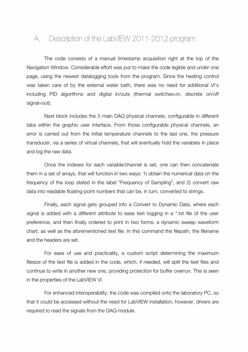
A. Description of the LabVIEW 2011-2012 program.

The code consists of a manual timestamp acquisition right at the top of the

Navigation Window. Considerable effort was put to make the code legible and under one

page, using the newest datalogging tools from the program. Since the heating control

was taken care of by the external water bath, there was no need for additional VI’s

including PID algorithms and digital in/outs (thermal switches=in, discrete on/off

signal=out).

Next block includes the 5 main DAQ physical channels, configurable in different

tabs within the graphic user interface. From those configurable physical channels, an

error is carried out from the initial temperature channels to the last one, the pressure

transducer, via a series of virtual channels, that will eventually hold the variables in place

and log the raw data.

Once the indexes for each variable/channel is set, one can then concatenate

them in a set of arrays, that will function in two ways: 1) obtain the numerical data on the

frequency of the loop stated in the label “Frequency of Sampling”, and 2) convert raw

data into readable floating-point numbers that can be, in turn, converted to strings.

Finally, each signal gets grouped into a Convert to Dynamic Data, where each

signal is added with a different attribute to ease text logging in a *.txt file of the user

preference, and then finally ordered to print in two forms: a dynamic sweep waveform

chart, as well as the aforementioned text file. In this command the filepath, the filename

and the headers are set.

For ease of use and practicality, a custom script determining the maximum

filesize of the text file is added in the code, which, if needed, will split the text files and

continue to write in another new one, providing protection for buffer overrun. This is seen

in the properties of the LabVIEW VI.

For enhanced interoperability, the code was compiled onto the laboratory PC, so

that it could be accessed without the need for LabVIEW installation, however, drivers are

required to read the signals from the DAQ-module.

Appendix C.

HSC Calculation – Example

Equilibrium Calculation (Isothermic)

Example Equilibrium Calculation (Isothermic)31 October 2012 10:09

Appendix A Page 1 Appendix A Page 2



Appendix A Page 23

Appendix D.

Mathematica Calculations

(*-----------Begin Program to Calculate Equilibrium------------*) TCel =25; T=TCel + 273.15; Barpressure =1.2; Pressure = Barpressure * 0.987; H2OIN =8.3; SO2IN =0.3; O2IN = 0.10; H2SO4IN=0.01; If[(T-273)≤50,do = (1.0-4.8*10-6*(T-273)2)]; If[(T-273)>50, do = (1.0064-(2.5*10-4*(T-273))-(2.3*10-6*(T-273)2))]; alphaSO2 = -0.030; elec = 4.8029*10-10; Dielec = 305.7*Exp[-Exp[-12.741+0.01875*T]-(T/219)]; k =1.38045*10-16; Mw = 0.01802; Na = 6.0232*1023; PSH2O = (10^(7.96681-1668.21/(T-45.15)))/760; R = 82.06; rH = 3.8; rHSO3 = 2.7; rOH = 3.5; rSO3 = 2.8; zH = 1; zHSO3 = -1; zOH = -1; zSO3 = -2; Subst = {KSO2, KH2O, KHSO3}; kvalA = {-3768, -13445.9, 1333.4}; kvalB = {-20,-22.4773,0}; kvalC={0.0,0 , 0}; kvalD={122.53, 140.932, -21.274}; Kvalue = Exp[(kvalA/T)+(kvalB*Log[T]) + (kvalC*T)+kvalD]; KSO2 =Kvalue[[1]]; KH2O = Kvalue[[2]]; KHSO3 =Kvalue[[3]]; HenvalA =6211.22; HenvalB = 60.239; HenvalC = -0.102974; HenvalD = -333.362; HenrySO2 = Exp[(HenvalA/T)+(HenvalB*Log[T]) + (HenvalC*T) + HenvalD]; vstar2= 115.0; vmolwater = 18.02*(1.001508+3.976412*10-6*(T-273.15)2); If[(T-273)≤50,ρ = 1.0-4.8*10-6*(T-273)2]; If[(T-273)>50, ρ = 1.0064-(2.5*10-4*(T-273))-(2.3*10-6*(T-273)2)]; Clear[C12subso, solution, solution1, solution2, K, partmolvol]; rhotil = ρ/18.012*46.4; solution1 =Solve[Log[1 +18.02/((ρ)*K*R*T)]�(-0.42704*(rhotil-1)+2.089*(rhotil-1)2-0.42367*(rhotil-1)3), K]; Flatten[solution1]; K = K/.solution1[[1]]; If[2≤rhotil≤2.785, series= -2.4467+ 2.12074*rhotil, "outside range"]; If[2.785≤rhotil≤3.2, series = 3.02214 - 1.87085*rhotil+0.71955*rhotil2, "outside range"]; For[i=2, i<3, ivalue = i; C12subso = (Subscript[vstar, ivalue]/46.4)0.62*(-Exp[series]); vmol ivalue= K*R*T*(1-C12subso)

i++]; partmolvolSO2 = vmol2/1000; partmolvolH2O = vmolwater/1000; partmolvolH = -0.0047; partmolvolHSO3 = 0.035; partmolvolOH = 0.0005; partmolvolSO3 = 0.0197; Ionicstrength =0.5*(molalH + molalOH + molalHSO3 + 4*molalSO3);

A = * ;

FAC=(-(A/3))*( /(1+1.2* )+2.0/1.2*Log[1+1.2*

]); Clear[Bi, Bypi, Bwateri]; Beta0 = {0.04, -0.06, 0.12}; Beta1 = {0.12, -0.54, 1.08}; ion= {1,2,3}; Bi[Beta0_, Beta1_, ion_] := (Beta0) + (Beta1)/(2*Ionicstrength)*(1-(1+2*Sqrt[Ionicstrength])*Exp[-2*Sqrt[Ionicstrength]]); Bypi [Beta0_, Beta1_, ion_] :=(Beta1)*(1-(1+2*Sqrt[Ionicstrength]+2*Ionicstrength)*Exp[(-2*Sqrt[Ionicstrength])]); Bwateri [Beta0_, Beta1_, ion_] := Beta0 +Beta1*Exp[-2*Sqrt[Ionicstrength]]; Bi = Bi[Beta0, Beta1, ion]; Bypi = Bypi[Beta0, Beta1, ion]; Bwateri = Bwateri[Beta0, Beta1, ion]; B1 = Bi[[1]]; Byp1 = Bypi[[1]]; Bwater1 = Bwateri[[1]]; B2 = Bi[[2]]; Byp2 = Bypi[[2]]; Bwater2 = Bwateri[[2]]; B3 = Bi[[3]]; Byp3 = Bypi[[3]]; Bwater3 = Bwateri[[3]]; Bsum = 2*molalH*((molalOH*Byp1)+(molalHSO3*Byp2)+(molalSO3*Byp3)); do; Vm = (1/do)+molalSO2*partmolvolSO2; Vi = (1/do)+(molalH*partmolvolH) +(molalOH*partmolvolOH)+ (molalHSO3*partmolvolHSO3)+ (molalSO3*partmolvolSO3); vHc = (4/3)*π*Na*(rH^3)*(10^-27); vOHc = (4/3)*π*Na*(rOH^3)*(10^-27) ; vHSO3c = (4/3)*π*Na*(rHSO3^3)*(10^-27); vSO3c = (4/3)*π*Na*(rSO3^3)*(10^-27); Vc = (molalH*vHc) + (molalOH * vOHc) + (molalHSO3*vHSO3c)+(molalSO3*vSO3c); Vf = Vi+(molalSO2*partmolvolSO2); lambdaSO2 = -0.05+(0/T); muSO2 = -(1/55.5)*(lambdaSO2+(1/166.5)); Ds = Dielec*(1+((alphaSO2*molalSO2)/Vm)); LH = ((elec^2)* (zH^2))/(2*rH*k*T*Dielec)*(10^8); LHSO3 = ((elec^2)* (zHSO3^2))/(2*rHSO3*k*T*Dielec)*(10^8); LOH = ((elec^2)* (zOH^2))/(2*rOH*k*T*Dielec)*(10^8); LSO3 = ((elec^2)* (zSO3^2))/(2*rSO3*k*T*Dielec)*(10^8); DIV = Dielec/Ds; Vfc = Vf - Vc; Vic = Vi - Vc; SUML = (molalH*LH)+ (molalOH*LOH)+ (molalHSO3*LHSO3)+(molalSO3*LSO3); BRAC = (DIV * molalSO2)*(-alphaSO2/Vm*(Vi+(0.5*Vc))/Vic-(1.5*partmolvolSO2*Vc)/(Vic*Vfc)); activitycoeffH = Exp[FAC+2*((molalOH*B1)+(molalHSO3*B2)+(molalSO3*B3))- (Bsum/(4*Ionicstrength2))+(BRAC*LH) + (1.5*SUML*((DIV*((Vf*vHc)-(Vc*partmolvolH))/Vfc2)-(((Vi*vHc)-(Vc*partmolvolH))/Vic2)))]; activitycoeffOH = Exp[FAC + (2*B1*molalH)-(Bsum/(4*Ionicstrength2))+(BRAC*LOH) + 1.5*SUML*(DIV*((Vf*vOHc)-(Vc*partmolvolOH))/Vfc2-((Vi*vOHc)-(Vc*partmolvolOH))/Vic2)]; activitycoeffHSO3 = Exp[FAC + (2*B2*molalH)-(Bsum/(4*Ionicstrength2))+(BRAC*LHSO3) + (1.5*SUML*((DIV*((Vf*vHSO3c)-(Vc*partmolvolHSO3))/Vfc2)-(((Vi*vHSO3c)-(Vc*partmolvolHSO3))/Vic2)))]; activitycoeffSO3 = Exp[(4*FAC) + (2*B3*molalH)-(Bsum/Ionicstrength2)+(BRAC*LSO3) + (1.5*SUML*((DIV*((Vf*vSO3c)-(Vc*partmolvolSO3))/Vfc2)-(((Vi*vSO3c)-(Vc*partmolvolSO3))/Vic2)))];

2∗ π∗ Na∗do

1000

12

elec2

Dielec∗k∗T

32

Ionicstrength Ionicstrength

Ionicstrength

activitycoeffSO2 = Exp[(2*lambdaSO2*molalSO2)+ (3*muSO2*molalSO22)+(SUML*DIV*(((-1.5*partmolvolSO2*Vc)/Vfc2)+(((Vf + (0.5*Vc))/Vfc)*(partmolvolSO2/Vm-(DIV*(partmolvolSO2+alphaSO2))/Vm))))];

activityH2O = Exp[Mw*(((2*A)/3*Ionicstrength1.5/(1 + 1.2* ))-(2*molalH*(Bwater1*molalOH +Bwater2*molalHSO3+ Bwater3*molalSO3))-(lambdaSO2*molalSO22)-(2*muSO2*molalSO23)-(molalH+molalOH+molalHSO3 +molalSO3+molalSO2)-(SUML*(((-alphaSO2*molalSO2*DIV2)/(do*Vm2)*(Vf+(0.5*Vc))/Vfc)+((1.5*Vc*DIV)/(do*Vfc2))-((1.5*Vc)/(do*Vic2)))))]; (αô)1,1= 0; (αô)2,2 = 0; (αô)1,2 = 1.7; (αô)2,1 = 1.7; c1=0.01; c2 = 0.017; αlp1 =3.1307; αlp2 = 2.8730; βeta1 =1161.7; βeta2 = 1815.4; γ1 =1.5589; γ2 = 1.1043; δ1 =0.593*10-4; δ2 = 2.721*10-4; (α^0)1=1.06; (α^0)2=2.86; (α^1)1=2.07; (α^1)2=0.01; (β^0)1=8.4; (β^0)2=21.9; (β^1)1=1153.3; (β^1)2=1793.5; Rl . atm = 0.082054; Initguess = ((Rl . atm*T)/Pressure); NVFUG = 2; f1= 1; PartpressureH2O =( (10^(7.96681-1668.21/(T-45.15)))/760); PartpressureSO2 = Pressure - PartpressureH2O; vapmolefracH2O = PartpressureH2O/Pressure; vapmolefracSO2 = 1 -vapmolefracH2O; y1 1= vapmolefracH2O; y12 = vapmolefracSO2; TOTY = y1 1+ y12; y1 = y11/ TOTY; y2 = y12/TOTY; Tempa = T; Pressa = Pressure; Clear[V, ETA]; Do[bi = Exp[2.30259*(-γi-δi*Tempa)];, {i, NVFUG}]; Do[ Do[ (β^0i,j)= 0.5*((β^0)i+(β^0)j); (β^1i,j)= Sqrt[(β^1)i*(β^1)j]; If [i�j ,(βi,j)=βetai, (βi,j)= (β^0i,j)+ (β^1i,j)]; (α^1i,j)= Sqrt[(α^1)i*(α^1)j]; If [i�j ,(αi,j)=αlpi, (αi,j)= (αô)i,j+ (α^1i,j)]; ai,j= αi,j + (βi,j)/T; , {j,1, NVFUG}]; , {i, 1,NVFUG}];

aM = ;

bM= ;

cM = ; ETA = bM/(4*V); VLO = bM/(4*1.0000001);

Ionicstrength

‚i=1

NVFUG

‚j=1

NVFUG

yi ∗ yj ∗ ai,j

‚i=1

NVFUG

yi ∗ bi

‚i=1

NVFUG

yi ∗ci

VHI = Initguess * 100; VIER = Solve[Pressure==(Rl . atm*T)/V*((1+ETA+ETA2-ETA3)/(1-ETA)3)-aM/(V(V+cM )), V]; Len = Length[VIER]; Do[Vsubs=V/.VIER[[subs]], {subs, 1, Len}]; V = Max[Table[Re[Vsubs], {subs, 1, Len}]]; z =( Pressure* V)/(Rl . atm * T); Do[fk= Exp[((4*ETA - 3*ETA2)/(1-ETA)2) +( bk/bM*((4*ETA - 2*ETA2)/(1-ETA)3))-(2/(Rl .

atm*T*V)*( ) *( +1))+((aM*ck)/(Rl . atm*T*V2)*(

+0.5))-Log[z]], {k,1, NVFUG}]; NVFUG = 1; y1 1= 1; y12 = 0; TOTY = y1 1+ y12; y1 = y11/ TOTY; y2 = y12/TOTY; Tempa = T; Pressa = Pressure; Clear[waterV, ETA]; Do[bi = Exp[2.30259*(-γi-δi*Tempa)];, {i, NVFUG}]; Do[ Do[ (β^0i,j)= 0.5*((β^0)i+(β^0)j); (β^1i,j)= Sqrt[(β^1)i*(β^1)j]; If [i�j ,(βi,j)=βetai, (βi,j)= (β^0i,j)+ (β^1i,j)]; (α^1i,j)= Sqrt[(α^1)i*(α^1)j]; If [i�j ,(αi,j)=αlpi, (αi,j)= (α^o)i,j+ (α^1i,j)]; ai,j= αi,j + (βi,j)/T; , {j,1, NVFUG}]; , {i, 1,NVFUG}];

aM = ;

bM= ;

cM = ; Clear[waterV]; ETA = bM/(4*waterV); BOX =( 1 + ETA + ETA2+ETA3)/(1-ETA)3; VVIER = Solve[Pressure == ((Rl . atm*T)/waterV*BOX) - aM/(waterV*(waterV+cM)), waterV]; Len = Length[VVIER]; Do[waterVsubs=waterV/.VVIER[[subs]], {subs, 1, Len}]; waterV= Max[Table[Re[waterVsubs], {subs, 1, Len}]]; purez =( Pressure* waterV)/(Rl . atm * T); fpurewater= Exp[((4*ETA - 3*ETA2)/(1-ETA)2) +( b1/bM*((4*ETA - 2*ETA2)/(1-ETA)3))-(2/(Rl .

atm*T*waterV)*( ) *( +1))+((aM*c1)/(Rl . atm*T*waterV)*(

+0.5))-Log[purez]]; fugcoeffpureH2O = f1purewater; guesspartpressureH2O =( (10^(7.96681-1668.21/(T-45.15)))/760)*1; Clear[vapmolefracSO2,vapmolefracH2O]; guessvapmolefracH2O = guesspartpressureH2O/Pressure; guessvapmolefracSO2 = 1 - guessvapmolefracH2O; guessmolesH2O = H2OIN; guessmolalH = 0.9*10-1; guessmolalOH = KH2O/guessmolalH; guessmolalSO2 = 0.05*(SO2IN); guessmolalHSO3 =(KSO2*guessmolalSO2)/(guessmolalH); guessmolalSO3 = (KHSO3*guessmolalHSO3)/(guessmolalH);

‚j=1

NVFUG

yj ∗ak,j ‚m=1

5 H−1Lm

m + 1∗KcM

VOm

‚m=1

4 H−1Lm ∗Hm + 1LHm + 2L ∗KcM

VOm

‚i=1

NVFUG

‚j=1

NVFUG

yi ∗ yj ∗ ai,j

‚i=1

NVFUG

yi ∗ bi

‚i=1

NVFUG

yi ∗ci

‚j=1

NVFUG

yj ∗a1,j ‚m=1

5 H−1Lm

m + 1∗K cM

waterVOm

‚m=1

4 H−1Lm ∗Hm + 1LHm + 2L ∗K cM

waterVOm

guessVaprate= 3; S1=KH2O==(activitycoeffH * molalH *activitycoeffOH * molalOH)/(activityH2O); S2 =KSO2 ==((activitycoeffH*molalH * activitycoeffHSO3 * molalHSO3)/(activitycoeffSO2 *molalSO2*activityH2O)); S3 =KHSO3== ((activitycoeffH*molalH * activitycoeffSO3 * molalSO3)/(activitycoeffHSO3 *molalHSO3)); (* Vapour liquid equilibria expressions labelled as book *) S5 = vapmolefracH2O * f1 *Pressure ==activityH2O* PSH2O * fugcoeffpureH2O*Exp[(partmolvolH2O *1000*(Pressure- PSH2O))/(R*T)]; S6 = vapmolefracSO2 * f2 * Pressure == molalSO2*activitycoeffSO2*HenrySO2* Exp[(partmolvolSO2 *1000*(Pressure- PSH2O))/(R*T)]; (*---------------------------------------------------------------------------------------*) (* other system equations*) (* vapour phase balance *) S8 = vapmolefracSO2 + vapmolefracH2O == 1; (* sulphur balance *) S9 = (molesH2O/55.51*(molalSO2 + molalHSO3 + molalSO3)) + (vapmolefracSO2*Vaprate) == SO2IN ; (* hydrogen balance *) S10 = (2*molesH2O) + (molesH2O/55.51*(molalH + molalOH + molalHSO3)) + (2*vapmolefracH2O*Vaprate)==2*H2OIN ; (* electroneutrality *) S11 = molalH == (molalOH + molalHSO3 + (2*molalSO3)); Unknowns= FindRoot[ {S1, S2, S3, S5,S6,S8, S9,S10,S11}, {{molesH2O, guessmolesH2O,10}, {molalH, guessmolalH,1}, {molalOH, guessmolalOH,1}, {molalSO2, guessmolalSO2,10}, {molalHSO3, guessmolalHSO3,1}, {molalSO3, guessmolalSO3,1}, {vapmolefracH2O, guessvapmolefracH2O,1}, {vapmolefracSO2, guessvapmolefracSO2,1}, {Vaprate, guessVaprate,5}},Method→"Secant"]; molesH2O = molesH2O/.Unknowns; molalH = molalH/.Unknowns; molalOH = molalOH/.Unknowns; molalSO2 = molalSO2/.Unknowns; molalHSO3 = molalHSO3/.Unknowns; molalSO3 = molalSO3/.Unknowns; vapmolefracH2O = vapmolefracH2O/.Unknowns; vapmolefracSO2 = vapmolefracSO2/.Unknowns; Vaprate= Vaprate/.Unknowns; molalHSO4=molalHSO3; molalSO4=molalSO3; vapmolefracO2=1-vapmolefracH2O-vapmolefracSO2+0.01; molalSO2aq=molalSO3+molalHSO3-.1; molalSO3aq=molalSO3*0.001; molalH2SO4aq=molalHSO4+molalSO4+.02; (*-----------Do Not Clear Variables------------*) (* (* Clear the values for Vapour Mole Fractions *) Clear[vapmolefracO2, vapmolefracSO3, vapmolefracSO2, vapmolefracH2SO4, vapmolefracH2O]; (* Clear the values for Ion Mole values *) Clear[molalH, molalOH, molalHSO3, molalHSO4, molalSO3, molalSO4]; (* Clear the values for Liquid Mole values *) Clear[molesSO2, molesH2O, molesO2, molesSO3, molesH2SO4, molalSO3aq, molalSO2aq, molalH2SO4aq]; (* Clear the values for K Values *) Clear[KH2O, KH2SO4, KHSO4, KH2SO4G, KSO3, KSO2,KHSO3]; (* Clear the values for Partial Molar Volumes*) Clear[partmolvolH2SO4, partmolvolH2O, partmolvolO2, partmolvolSO3, partmolvolSO2]; (* Clear the values for Partial Pressures*) Clear[vapmolefracH2SO4, vapmolefracH2O, vapmolefracO2, vapmolefracSO3, vapmolefracSO2] (* Clear the values for the other necessary variables*)

Clear[ρ,Subst,Vaprate, IonicStrength,Totpress, TotalMolalH2SO4, TotalMolalSO2, TotalMolalSO3];*) Pressure = Barpressure * 0.987; T=TCel + 273.15; guesspartpressureH2O =Pressure*.1; guesspartpressureSO2 =Pressure*.5*SO2IN; guesspartpressureO2 = Pressure - (guesspartpressureH2O + guesspartpressureSO2+guesspartpressureH2SO4 ); guesspartpressureH2SO4 =Pressure*.01*H2SO4IN; (*---------------------Define Constants-----------------------------------------*) If[(T-273)≤50,do = (1.0-4.8*10-6*(T-273)2)]; If[(T-273)>50, do = (1.0064-(2.5*10-4*(T-273))-(2.3*10-6*(T-273)2))];(*Density of Water*) alphaSO2 = -0.030; alphaSO3 = -0.030;(*added*) alphaH2SO4 = -0.030;(*added*) elec = 4.8029*10-10; Dielec = 305.7*Exp[-Exp[-12.741+0.01875*T]-(T/219)]; k =1.38045*10-16;(*Boltzmann Constant*) Mw = 0.01802;(*MW of Water*) Na = 6.0232*1023;(*Avogadros Number*) PSH2O = (10^(7.96681-1668.21/(T-45.15)))/760;(*Vapour Pressure of Water*) R = 82.06;(*Gas Constant, need units*) (*Ionic Radius - Check Numbers of sulfate and bisulfate*) rH = 3.8; rHSO3 = 2.7; rOH = 3.5; rSO3 = 2.8; rHSO4 = 2.7; rSO4 = 2.8; (*Electric Charge*) zH = 1; zHSO3 = -1; zOH = -1; zSO3 = -2; zHSO4 = -1; zSO4 = -2; (*-------------------------------------------------------------*) (*-------------------------------------------------------------*) (* Calculation of equilibrium constants for liquid phase reactions The order is the following: 1=SO2 dissociation 2=Water hydrolysis 3=Bisulphite formation 4=Sulphuric Acid Strong dissociation 5=Bisulfate formation 6=Sulfuric acid formation *) (* Substituted K values for values within property databanks *) (* Subst = {KSO2, KH2O, KHSO3, KH2SO4, KHSO4, KSO3, KH2SO4G}; kvalA = {-3768, -13445.9, 1333.4,1333.4,1333.4,1333.4,1333.4}; kvalB = {-20,-22.4773,0,0,0,0,0}; kvalC={0.0,0 , 0,0,0,0,0}; kvalD={122.53, 140.932, -21.274, -21.274, -21.274, -21.274, -21.274}; Kvalue = Exp[(kvalA/T)+(kvalB*Log[T]) + (kvalC*T)+kvalD]; (*Print["Equilibrium constants for liquid phase reactions"]*) KSO2 =Kvalue[[1]]; KH2O = Kvalue[[2]]; KHSO3 =Kvalue[[3]]; KH2SO4 =Kvalue[[4]]; KHSO4 =Kvalue[[5]]; KSO3 =Kvalue[[6]]; KH2SO4G =Kvalue[[7]]; *) (*These values are fitted from the HSC rate bank - Reaction Equations - Correct if needed*) KSO2 =N[3*10^(-6)*TCel*TCel-0.0006*TCel+0.0292];

KH2O =N[9*10^(-17)*TCel*TCel-5*10^(-15)*TCel+9*10^(-14)]; KHSO3 =N[3*10^(-12)*TCel*TCel-1*10^(-9)*TCel+9*10^(-8)]; KH2SO4 =N[3*10^(12)*Exp[-0.089*TCel]]; KHSO4 =N[2*10^(-6)*TCel^2-0.0004*TCel+0.0183]; KSO3 =N[9*10^(-15)*Exp[0.1245*TCel]];(*Formation of acid under trioxide dissolution*) KH2SO4G =N[3*10^(-11)*Exp[0.111*TCel]]; (*-------------------------------------------------------------*) (*Calculation of ionic quantities for activity coefficient calculation*) (* litwater=H2OIN*Mw/do; Print["Liters of water: ", litwater]; contribH1=Sqrt[KH2O]; molalO2=Sqrt[KH2O]; molalHSO3= *) (*-------------------------------------------------------------*) (*Calculation of Henry's constant for Subscript[SO, 2]*) HenvalA =6211.22; HenvalB = 60.239; HenvalC = -0.102974; HenvalD = -333.362; HenrySO2 = Exp[(HenvalA/T)+(HenvalB*Log[T]) + (HenvalC*T) + HenvalD]; (*Print["Calculated Henry's Constant = ", HenrySO2];*) (*------------------------------------------------------------------------*) (*Calculation of Henry's constant for Subscript[SO, 3] - INCORRECT VALUES*) HenvalA =6211.22; HenvalB = 60.239; HenvalC = -0.102974; HenvalD = -333.362; HenrySO3 = Exp[(HenvalA/T)+(HenvalB*Log[T]) + (HenvalC*T) + HenvalD]; (*------------------------------------------------------------------------*) (*Calculation of Henry's constant for Subscript[H, 2] Subscript[SO, 4] - INCORRECT VALUES*) HenvalA =6211.22; HenvalB = 60.239; HenvalC = -0.102974; HenvalD = -333.362; HenryH2SO4 = Exp[(HenvalA/T)+(HenvalB*Log[T]) + (HenvalC*T) + HenvalD]; (*------------------------------------------------------------------------*) (* Calculation of Henry's Constant for O2 *) KHdash = Exp[1/(8.3144*T) ((0.046*T2)+(203.357*T*Log[T/298])-((299.378+0.092*T)*(T-298))-20.591*103)]; HenryO2 = 1/KHdash; (* Print["Calculated Henry's Constant = ", HenryH2SO4]; Print["Calculated Henry's Constant Subscript[O, 2] = ", HenryO2]; Print["Calculated Henry's Constant = ", HenrySO3]; *) (* ---------------------------------------------------------------------- *) (*Brelvi & O'Connell Correlation for Partial Molar volume*) (* vsubso = partial molar volume at infinite dilution, cm^3/g mole (Overscript[v, _]^o); R = gas constant, 82.06 atm cm^3/g mole K (R); T = Temperature, Kelvins; C12subso = reduced volume integral of the molecular direct correlation function Subscript[c, ij] at infinite dilution (Subscript[C, 12]^o);

K2subso = isothermal compressibility at infinite dilution, atm^-1 (Subscript[K, 2]^o); vistar = characteristic volume of i, cm^3/g mole. For nonpolar species the critical volume, Subscript[v, c], may be used; experimental compressibility data may be used to determaine v^* for polar compounds. (Subscript[v, i]^*); rho = pure solvent density, g mole/cm^3 (ρ); rhotil = reduced density = Subscript[ρv, 2]^* (Overscript[ρ, ~]); *) (* the numbers 1 2 and 3 are the opposite way round to the book *) (* 1 - water *) (* 2 - sulphur dioxide *) (* 3 - oxygen *) (* 4 - sulphur trioxide *) (* 5 - sulfuric acid *) (*vstar and molecular weight Linear Solution - see Vstar Calculation*) (*END vstar and molecular weight Linear Solution*) (* vstar values from Zemaitis *) vstar1= 46.4; vstar2= 115.0; vstar3 = 74.4; vstar4= 132; vstar5= 154; (* the molar volume of water is calculated using this equation *) vmolwater = 18.02*(1.001508+3.976412*10-6*(T-273.15)2); (*Calculation of density of water using equation from Handbook*) If[(T-273)≤50,ρ = 1.0-4.8*10-6*(T-273)2]; If[(T-273)>50, ρ = 1.0064-(2.5*10-4*(T-273))-(2.3*10-6*(T-273)2)]; Clear[C12subso, solution, solution1, solution2, K, partmolvol]; rhotil = ρ/18.012*46.4; solution1 =Solve[Log[1 +18.02/((ρ)*K*R*T)]�(-0.42704*(rhotil-1)+2.089*(rhotil-1)2-0.42367*(rhotil-1)3), K]; Flatten[solution1]; K = K/.solution1[[1]]; If[2≤rhotil≤2.785, series= -2.4467+ 2.12074*rhotil, "outside range"]; If[2.785≤rhotil≤3.2, series = 3.02214 - 1.87085*rhotil+0.71955*rhotil2, "outside range"]; For[i=2, i<6, ivalue = i; C12subso = (Subscript[vstar, ivalue]/46.4)0.62*(-Exp[series]); vmol ivalue= K*R*T*(1-C12subso); i++] partmolvolSO2aq = vmol2/1000; partmolvolSO2 = vmol2/1000; partmolvolH2O = vmolwater/1000; partmolvolO2 = vmol3/1000; partmolvolSO3aq = vmol4/1000; partmolvolH2SO4 = vmol5/1000; (*Print["Calculated partial molar volumes"] Print["Partial molar volume of SO2 = ", partmolvolSO2, " dm3/mol"] Print["Partial molar volume of H2O = ", partmolvolH2O, " dm3/mol"] Print["Partial molar volume of O2 = ", partmolvolO2, "dm3/mol"] Print[] Print["in zemaitis the henry's law equation says these should be in dm3 per mole but then in the calculations they give cm3 per mole and analysis of the exponential term would indicate that cm3 mol is the appropriate unit, need to calculate in dm3 for the activity coefficient equations though"] Print[]*) (* rest of partial molar volumes from table in appendix 9.1 Zemaitis - Check Partial Molar Volumes*) partmolvolH = -0.0047; partmolvolHSO3 = 0.035; partmolvolOH = 0.0005; partmolvolSO3 = 0.0197; partmolvolHSO4 = 0.035*1.2;

partmolvolSO4 = 0.035*1.2; (* partial molar volume of oxygen in water from Bignell J Phys Chem 1984, 88, 5409 - 5412 *) partmolvolO2bignell = (31.73 - 0.0919*TCel + 0.00267*(TCel^2))/1000; (* Print["Partial molar volume of O2 from bignell = ", partmolvolO2bignell, " m^3 mol^-1"]; *) (* Bignells paper had an incorrect unit the value given by Brelvi and O'Connell is in the right unit *) (* partial molar volume is the contribution that a component makes to the total volume of a sample partial molar volume of a substance A in a mixture is the change in volume on the addition of 1 mol A to a large excess of the mixture *) (* Zhou and Battino gave the partial molar volume of oxygen as 32 cm3 mol-1 *) (*-------------------------------------------------------------*) (* Calculation of fugacity coefficients for each species using Nakamura equation of state *) (*<<Miscellaneous`RealOnly`*) (* Define constants; 1 = water, 2 = sulphur dioxide 3 = oxygen , 4 = sulfur trioxide, 5 = sulphuric acid THESE ARE ALL FAKE*) (αô)1,1= 0; (αô)1,2 = 1.7; (αô)1,3 = 2.19; (αô)1,4 = 2.19; (αô)1,5 = 2.19; (αô)2,1 = 1.7; (αô)2,2 = 1; (αô)2,3 = 2; (αô)2,4 = 1; (αô)2,5 =1; (αô)3,1 = 2.19; (αô)3,2 = 2; (αô)3,3 = 2; (αô)3,4 = 2; (αô)3,5 = 2; (αô)4,1 = 2; (αô)4,2 = 2; (αô)4,3 = 2; (αô)4,4 = 4; (αô)4,5 = 4; (αô)5,1 = 3; (αô)5,2 = 3; (αô)5,3 = 3; (αô)5,4 = 4; (αô)5,5 = 5; c1=0.01; c2 = 0.017; c3 = 0; c4 = .017; c5 = 0; αlp1 =3.1307; αlp2 = 2.8730; αlp3 = 1.5324; αlp4 = 1.5324; αlp5 = 1.5324; βeta1 =1161.7; βeta2 = 1815.4; βeta3 = 8.56; βeta4 = 8.56; βeta5 = 8.56; γ1 =1.5589;

γ2 = 1.1043; γ3 = 1.2458; γ4 =1.5589; γ5 =1.5589; δ1 =0.593*10-4; δ2 = 2.721*10-4; δ3 = 1.199*10-4; δ4 = 1.199*10-4; δ5 = 1.199*10-4; (* nonpolar and polar contributions *) (α^0)1=1.06; (α^0)2=2.86; (α^0)3=1.5324; (α^0)4=1.5324; (α^0)5=1.5324; (α^1)1=2.07; (α^1)2=0.01; (α^1)3=0.0; (α^1)4=0.0; (α^1)5=0.0; (β^0)1=8.4; (β^0)2=21.9; (β^0)3=8.56; (β^0)4=8.56; (β^0)5=8.56; (β^1)1=1153.3; (β^1)2=1793.5; (β^1)3=0; (β^1)4=0; (β^1)5=0; (* ---------------- Calculation of fugacity coefficients ----------------------- *) Rl . atm = 0.082054; Initguess = ((Rl . atm*T)/Pressure); NVFUG = 5; (* 1 = water, 2 = sulphur dioxide, 3 = oxygen , 4= SO3, 5=H2SO4*) guessvapmolefracH2O = guesspartpressureH2O/Pressure; guessvapmolefracSO2 = guesspartpressureSO2/Pressure; guessvapmolefracO2 = guesspartpressureO2/Pressure; guessvapmolefracSO3 = guesspartpressureSO2/Pressure*.075; guessvapmolefracH2SO4 = guesspartpressureH2SO4/Pressure; y11= guessvapmolefracH2O; y12 = guessvapmolefracSO2; y13 = guessvapmolefracO2; y14 = guessvapmolefracSO3; y15 = guessvapmolefracH2SO4; TOTY = y1 1+ y12 + y13+y14+y15; y1 = y11/ TOTY; y2 = y12/TOTY; y3=y13/TOTY; y4=y14/TOTY; y5=y15/TOTY; Tempa = T; Pressa = Pressure; Clear[V, ETA]; Do[bi = Exp[2.30259*(-γi-δi*Tempa)];, {i, NVFUG}]; Do[ Do[ (β^0i,j)= 0.5*((β^0)i+(β^0)j); (β^1i,j)= Sqrt[(β^1)i*(β^1)j]; If [i�j ,(βi,j)=βetai, (βi,j)= (β^0i,j)+ (β^1i,j)];

(α^1i,j)= Sqrt[(α^1)i*(α^1)j]; If [i�j ,(αi,j)=αlpi, (αi,j)= (α^o)i,j+ (α^1i,j)]; ai,j= αi,j + (βi,j)/T; , {j,1, NVFUG}]; , {i, 1,NVFUG}];

aM = ;

bM= ;

cM = ; ETA = bM/(4*V); VLO = bM/(4*1.0000001); VHI = Initguess * 100; (* Print["Initial Guess for Molar Volume from ideal gas law = ", Initguess]; Print["Molar volume boundary"]; Print["Possible highest value = ", VHI]; Print["Possible lowest value = ", VLO]; Print[]; *) VIER = Solve[Pressure==(Rl . atm*T)/V*((1+ETA+ETA2-ETA3)/(1-ETA)3)-aM/(V(V+cM )), V]; Len = Length[VIER]; Do[Vsubs=V/.VIER[[subs]], {subs, 5, Len}]; Vsol = Table[Vsubs, {subs, 5, Len}]; Vsol; V = Max[Vsol]; z =( Pressure* V)/(Rl . atm * T); Do[fk= Exp[((4*ETA - 3*ETA2)/(1-ETA)2) +( bk/bM*((4*ETA - 2*ETA2)/(1-ETA)3))-(2/(Rl .

atm*T*V)*( ) *( +1))+((aM*ck)/(Rl . atm*T*V2)*(

+0.5))-Log[z]], {k,1, NVFUG}]; (* Print["molar volume = ", V, " l/mole"] Print ["fugacity coefficient of water = ",Subscript[f, 1]]; Print["Fugacity coefficient of sulphur dioxide = ", Subscript[f, 2]]; Print["Fugacity coefficient of oxygen = ", Subscript[f, 3]]; Print["Fugacity coefficient of SO3 = ", Subscript[f, 4]]; Print["Fugacity coefficient of H2SO4 = ", Subscript[f, 5]]; *) (* ---------------------------------------*) (* ---------------------------------------*) (* calculation of pure water fugacity using Nakamura equation of state *) (* 1 = water, 2 = nothing *) NVFUG = 1; y1 1= 1; y12 = 0; TOTY = y1 1+ y12; y1 = y11/ TOTY; y2 = y12/TOTY; Tempa = T; Pressa = Pressure; Clear[waterV, ETA]; Do[bi = Exp[2.30259*(-γi-δi*Tempa)];

‚i=1

NVFUG

‚j=1

NVFUG

yi ∗ yj ∗ ai,j

‚i=1

NVFUG

yi ∗ bi

‚i=1

NVFUG

yi ∗ci

‚j=1

NVFUG

yj ∗ak,j ‚m=1

5 H−1Lm

m + 1∗KcM

VOm

‚m=1

4 H−1Lm ∗Hm + 1LHm + 2L ∗KcM

VOm

(*Print[SubscriptBox["b",i]//DisplayForm, " = ",Subscript[b, i] ];*), {i, NVFUG}]; Do[ Do[ (β^0i,j)= 0.5*((β^0)i+(β^0)j); (β^1i,j)= Sqrt[(β^1)i*(β^1)j]; If [i�j ,(βi,j)=βetai, (βi,j)= (β^0i,j)+ (β^1i,j)]; (α^1i,j)= Sqrt[(α^1)i*(α^1)j]; If [i�j ,(αi,j)=αlpi, (αi,j)= (α^o)i,j+ (α^1i,j)]; ai,j= αi,j + (βi,j)/T; , {j,1, NVFUG}]; , {i, 1,NVFUG}];

aM = ;

bM= ;

cM = ; Clear[waterV] ETA = bM/(4*waterV); BOX =( 1 + ETA + ETA2+ETA3)/(1-ETA)3; VVIER = Solve[Pressure == ((Rl . atm*T)/waterV*BOX) - aM/(waterV*(waterV+cM)), waterV]; Len = Length[VVIER]; Do[waterVsubs=waterV/.VVIER[[subs]], {subs, 5, Len}]; Vsol = Table[waterVsubs, {subs,5, Len}]; waterV = Max[Vsol]; (* Calculation of compressibility factor*) purez =( Pressure* waterV)/(Rl . atm * T); fpurewater= Exp[((4*ETA - 3*ETA2)/(1-ETA)2) +( b1/bM*((4*ETA - 2*ETA2)/(1-ETA)3))-(2/(Rl .

atm*T*waterV)*( ) *( +1))+((aM*c1)/(Rl . atm*T*waterV)*(

+0.5))-Log[purez]]; fugcoeffpureH2O = f1purewater; (*Print["fugacity coefficient for pure water = ", fugcoeffpureH2O]*) (* ------------------------------------------------------------------------- *) (* Calculation of activity coefficient of oxygen in sulphur dioxide electrolyte solution from UEA paper Clegg and Brimblecombe Modify with sulphuric Acid and Sulfur Trioxide*) λO2,H= -0.2379 + 81.450/T; λO2,OH= 0.93318 - 430.552/T+49860.8/T2; λO2,HSO3= (15.571/T)/2; λO2,SO3= 15.571/T; ζO2,H,OH=0; ζO2,H,HSO3=0; ζO2,H,SO3=0; activitycoeffO2 = Exp[(2*molalH*λO2,H) +2*((molalOH*λO2,OH) +(molalHSO3 * λO2,HSO3)+(molalSO3 *λO2,SO3))+((molalH*molalOH*ζO2,H,OH)+ (molalH*molalHSO3*ζO2,H,HSO3)+(molalH*molalSO3 * ζO2,H,SO3))]; (* ionic strength *) IonicStrength =0.5*(molalH + molalOH + molalHSO3 + 4*molalSO3+4*molalSO4+molalHSO4); (* Print["Ionic strength = ", IonicStrength]; *)

‚i=1

NVFUG

‚j=1

NVFUG

yi ∗ yj ∗ ai,j

‚i=1

NVFUG

yi ∗ bi

‚i=1

NVFUG

yi ∗ci

‚j=1

NVFUG

yj ∗a1,j ‚m=1

5 H−1Lm

m + 1∗K cM

waterVOm

‚m=1

4 H−1Lm ∗Hm + 1LHm + 2L ∗K cM

waterVOm

(*---------------------------------------------------------------*) (*---------------------------------------------------------------*) (* The Debye-Huckel constant, A, is calculated as follows *)

A = * ; (* Print["Debye-Huckel constant A = ", A]; *) (* Debye-Huckel term *)

FAC=(-(A/3))*( /(1+1.2* )+2.0/1.2*Log[1+1.2*

]); (* Print["Debye-Huckel term FAC = ", FAC]; *) (*---------------------------------------------------------------*) (*---------------------------------------------------------------*) (*ion-ion interactions using standard Pitzer terms*) Clear[Bi, Bypi, Bwateri]; (* species specific coefficients (water-sulphur dioxide system) values in order, H+OH-, H+HSO3-, H+SO3- , H+HSO4-, H+SO4-- INCORRECT DATA - MODIFY!*) Beta0 = {0.04, 0.06, 0.12, .02, .02}; Beta1 = {0.12, 0.54, 1.08, .02, .02}; ion= {1,2,3, 4, 5}; Bi[Beta0_, Beta1_, ion_] := (Beta0) + (Beta1)/(2*IonicStrength)*(1-(1+2*Sqrt[IonicStrength])*Exp[-2*Sqrt[IonicStrength]]); Bypi [Beta0_, Beta1_, ion_] :=(Beta1)*(1-(1+2*Sqrt[IonicStrength]+2*IonicStrength)*Exp[(-2*Sqrt[IonicStrength])]); Bwateri [Beta0_, Beta1_, ion_] := Beta0 +Beta1*Exp[-2*Sqrt[IonicStrength]]; Bi = Bi[Beta0, Beta1, ion]; Bypi = Bypi[Beta0, Beta1, ion]; Bwateri = Bwateri[Beta0, Beta1, ion]; B1 = Bi[[1]]; Byp1 = Bypi[[1]]; Bwater1 = Bwateri[[1]]; B2 = Bi[[2]]; Byp2 = Bypi[[2]]; Bwater2 = Bwateri[[2]]; B3 = Bi[[3]]; Byp3 = Bypi[[3]]; Bwater3 = Bwateri[[3]]; B4 = Bi[[4]]; Byp4 = Bypi[[4]]; Bwater4 = Bwateri[[4]]; B5 = Bi[[5]]; Byp5 = Bypi[[5]]; Bwater5 = Bwateri[[5]]; Bsum = 2*molalH*((molalOH*Byp1)+(molalHSO3*Byp2)+(molalSO3*Byp3)+(molalHSO4*Byp4)+(molalSO4*Byp5)); (*------------------------------------------------------------------------*) (*ion molecule interaction coefficients from dielectric effects*) do; (* Print["Density of water = ", do, " kg/dm^3"] *)

2∗ π∗ Na∗do

1000

12

elec2

Dielec∗k∗T

32

IonicStrength IonicStrength

IonicStrength

(* a. volume of neutral solution excluding ions, dm^3/kg of Subscript[H, 2]O / NOTE THAT THERE IS NO H2SO4!*) Vm = (1/do)+molalSO2aq*partmolvolSO2+molalSO3aq*partmolvolSO3aq; (* b. volume of ionic solution excluding neutral solutes, dm^3/kg Subscript[H, 2]O *) Vi = (1/do)+(molalH*partmolvolH) +(molalOH*partmolvolOH)+ (molalHSO3*partmolvolHSO3)+ (molalSO3*partmolvolSO3)+(molalSO4*partmolvolSO4)+(molalHSO4*partmolvolHSO4); (* c. volume of ionic cavities for ion i, dm/mole *) vHc = (4/3)*π*Na*(rH^3)*(10^-27); vOHc = (4/3)*π*Na*(rOH^3)*(10^-27) ; vHSO3c = (4/3)*π*Na*(rHSO3^3)*(10^-27); vSO3c = (4/3)*π*Na*(rSO3^3)*(10^-27); vHSO4c = (4/3)*π*Na*(rHSO4^3)*(10^-27); vSO4c = (4/3)*π*Na*(rSO4^3)*(10^-27); (* d. volume of all ionic cavities, dm^3/kg Subscript[H, 2]O *) Vc = (molalH*vHc) + (molalOH * vOHc) + (molalHSO3*vHSO3c)+(molalSO3*vSO3c)+(molalSO4*vSO4c)+(molalHSO4*vHSO4c); (* e. volume of real solution dm^3/kg Subscript[H, 2]O *) Vf = Vi+(molalSO2aq*partmolvolSO2)+(molalSO3aq*partmolvolSO3aq); (*----------------------------------------------------------------------------------*) (* molecule molecule interactions + CORRECT FOR SO3-SO3 and O2-O2?*) (*lambdaSO2 = 0.0275+(0/T)*) lambdaSO2 = -0.05+(0/T); muSO2 = -(1/55.5)*(lambdaSO2+(1/166.5)); (*SAME LAMBDA WITH SO2*) lambdaSO3 = -0.05+(0/T); muSO3 = -(1/55.5)*(lambdaSO3+(1/166.5)); muH2SO4=muSO3*3; (* What is this haha get rid of this!*) (*--------------Dielectric constant of soln without ions--------------------------*) Ds = Dielec*(1+(((alphaSO2*molalSO2aq)+(alphaSO3*molalSO3))/Vm)); (* ------------------------------------------------------------------ *) vapmolefracH2SO4=vapmolefracSO2*.1; vapmolefracSO3=vapmolefracSO2*01; (*--------------------------------------------------------------------------------*) (*dimensionless constant of dielectric contribution of ion i in activity coefficient*) LH = ((elec^2)* (zH^2))/(2*rH*k*T*Dielec)*(10^8); LHSO3 = ((elec^2)* (zHSO3^2))/(2*rHSO3*k*T*Dielec)*(10^8); LOH = ((elec^2)* (zOH^2))/(2*rOH*k*T*Dielec)*(10^8); LSO3 = ((elec^2)* (zSO3^2))/(2*rSO3*k*T*Dielec)*(10^8); LHSO4 = ((elec^2)* (zHSO4^2))/(2*rHSO4*k*T*Dielec)*(10^8); LSO4 = ((elec^2)* (zSO4^2))/(2*rSO4*k*T*Dielec)*(10^8); (*--------------------------------------------------------------------------------*) (*Definition of terms often used to simplify the activity coefficient equations*) DIV = Dielec/Ds; Vfc = Vf - Vc; Vic = Vi - Vc; SUML = (molalH*LH)+ (molalOH*LOH)+ (molalHSO3*LHSO3)+(molalSO3*LSO3); BRAC = (DIV * molalSO2aq)*(-alphaSO2/Vm*(Vi+(0.5*Vc))/Vic-(1.5*partmolvolSO2*Vc)/(Vic*Vfc)); (*-----------------------------------OXYGEN-----------------------------------*) Calcppoxygen = vapmolefracO2 * Barpressure; PartialO2bar = Calcppoxygen; PartialO2atm = PartialO2bar * 0.987; T =TCel + 273.15; conc = PartialO2atm*Exp[1/(8.3144*T) ((0.046*T2)+(203.357*T*Log[T/298])-((299.378+0.092*T)*(T-298))-20.591*103)]; (*--------------------------------------------------------------------------------*) (*ERASE AFTER THIS : DEBUGGING AREA*)

activitycoeffH = Exp[FAC+2*((molalOH*B1)+(molalHSO3*B2)+(molalSO3*B3))- (Bsum/(4*IonicStrength2))+(BRAC*LH) + (1.5*SUML*((DIV*((Vf*vHc)-(Vc*partmolvolH))/Vfc2)-(((Vi*vHc)-(Vc*partmolvolH))/Vic2)))]; (*----------------------------------------------------------------------------------*) (* OH- hydroxide ion activity coefficient *) activitycoeffOH = Exp[FAC + (2*B1*molalH)-(Bsum/(4*IonicStrength2))+(BRAC*LOH) + 1.5*SUML*(DIV*((Vf*vOHc)-(Vc*partmolvolOH))/Vfc2-((Vi*vOHc)-(Vc*partmolvolOH))/Vic2)]; (*----------------------------------------------------------------------------------*) (* HSO4- bisulphate ion activity coefficient - CORRECT?*) activitycoeffHSO4= Exp[FAC + (2*B2*molalH)-(Bsum/(4*IonicStrength2))+(BRAC*LHSO4) + (1.5*SUML*((DIV*((Vf*vHSO4c)-(Vc*partmolvolHSO4))/Vfc2)-(((Vi*vHSO4c)-(Vc*partmolvolHSO4))/Vic2)))]; (*----------------------------------------------------------------------------------*) (* HSO3- bisulphite ion activity coefficient *) activitycoeffHSO3 = Exp[FAC + (2*B2*molalH)-(Bsum/(4*IonicStrength2))+(BRAC*LHSO3) + (1.5*SUML*((DIV*((Vf*vHSO3c)-(Vc*partmolvolHSO3))/Vfc2)-(((Vi*vHSO3c)-(Vc*partmolvolHSO3))/Vic2)))]; (*----------------------------------------------------------------------------------*) (* SO3-- sulphite ion activity coefficient *) activitycoeffSO3 = Exp[(4*FAC) + (2*B3*molalH)-(Bsum/IonicStrength2)+(BRAC*LSO3) + (1.5*SUML*((DIV*((Vf*vSO3c)-(Vc*partmolvolSO3))/Vfc2)-(((Vi*vSO3c)-(Vc*partmolvolSO3))/Vic2)))]; (*----------------------------------------------------------------------------------*) (* SO4-- Sulphate Ion activity coefficient *) activitycoeffSO4 = Exp[(4*FAC) + (2*B3*molalH)-(Bsum/IonicStrength2)+(BRAC*LSO4) + (1.5*SUML*((DIV*((Vf*vSO4c)-(Vc*partmolvolSO4))/Vfc2)-(((Vi*vSO4c)-(Vc*partmolvolSO4))/Vic2)))]; (*----------------------------------------------------------------------------------*) (*SO2 Sulphur dioxide activity coefficient*) activitycoeffSO2 = Exp[(2*lambdaSO2*molalSO2aq)+ (3*muSO2*molalSO2aq2)+(SUML*DIV*(((-1.5*partmolvolSO2aq*Vc)/Vfc2)+(((Vf + (0.5*Vc))/Vfc)*(partmolvolSO2aq/Vm-(DIV*(partmolvolSO2aq+alphaSO2))/Vm))))]; (*----------------------------------------------------------------------------------*) (*SO3 Sulphur trioxide activity coefficient*) activitycoeffSO3aq = Exp[(2*lambdaSO3*molalSO3aq)+ (3*muSO3*molalSO3aq2)+(SUML*DIV*(((-1.5*partmolvolSO3aq*Vc)/Vfc2)+(((Vf + (0.5*Vc))/Vfc)*(partmolvolSO3aq/Vm-(DIV*(partmolvolSO3aq+alphaSO3))/Vm))))]; (*----------------------------------------------------------------------------------*) (*H2SO4 Sulfuric Acid activity coefficient*) activitycoeffH2SO4 = Exp[ (3*muH2SO4*molalH2SO4aq2)+(SUML*DIV*(((-1.5*partmolvolH2SO4*Vc)/Vfc2)+(((Vf + (0.5*Vc))/Vfc)*(partmolvolH2SO4/Vm-(DIV*(partmolvolH2SO4+alphaH2SO4))/Vm))))]; (*-----------------------------------------------------------------------------------*) (* Water activity *)

activityH2O = Exp[Mw*(((2*A)/3*IonicStrength1.5/(1 + 1.2* ))- (2*molalH*(Bwater1*molalOH +Bwater2*molalHSO3+ Bwater3*molalSO3+Bwater4*molalHSO4+Bwater5*molalSO4)) -(lambdaSO2*molalSO2aq2)-(lambdaSO3*molalSO32) -(2*muSO2*molalSO2aq3)-(2*muSO3*molalSO33) -(molalH+molalOH+molalHSO3 +molalSO3+molalSO2aq)-(SUML*(((-alphaSO2*molalSO2aq*DIV2)/(do*Vm2)*(Vf+(0.5*Vc))/Vfc)+((1.5*Vc*DIV)/(do*Vfc2))-((1.5*Vc)/(do*Vic2)))))]; (*-----------------------------------------------------------------------------*) (* Liquid phase reaction equations labelled as book *) S1=KH2O==(activitycoeffH * molalH *activitycoeffOH * molalOH)/(activityH2O); S2 =KSO2 ==((activitycoeffH*molalH * activitycoeffHSO3 * molalHSO3)/(activitycoeffSO2 *molalSO2aq*activityH2O));

IonicStrength

S3 =KHSO3== ((activitycoeffH*molalH * activitycoeffSO3 * molalSO3)/(activitycoeffHSO3 *molalHSO3)); S4 =KHSO4== ((activitycoeffH*molalH * activitycoeffSO4 * molalSO4)/(activitycoeffHSO4 *molalHSO4)); S5= KH2SO4 == ((activitycoeffH*molalH * activitycoeffHSO4 * molalHSO4)/(activitycoeffH2SO4 *molalH2SO4aq*activityH2O)); S6= KSO3 == ((activitycoeffH2SO4 * molalH2SO4aq)/(activitycoeffSO3aq *molalSO3aq*activityH2O)); (* Gas phase reaction equation *) S7 = KH2SO4G �(fugcoeffpureH2O*vapmolefracH2O*f4*vapmolefracSO3)/(f5*vapmolefracH2SO4); (* Vapour liquid equilibria expressions labelled as book *) S8 = vapmolefracH2O * f1 *Pressure ==activityH2O* PSH2O * fugcoeffpureH2O*Exp[(partmolvolH2O *1000*(Pressure- PSH2O))/(R*T)]; S9= vapmolefracSO2 * f2 * Pressure == molalSO2aq*activitycoeffSO2*HenrySO2* Exp[(partmolvolSO2 *1000*(Pressure- PSH2O))/(R*T)]; S10= vapmolefracO2 * f3 * Pressure � molalO2 * activitycoeffO2 * HenryO2 * Exp[(partmolvolO2*1000* (Pressure - PSH2O))/(R*T)]; S11= vapmolefracSO3 * f4 * Pressure � molalSO3aq * activitycoeffSO3aq * HenrySO3 * Exp[(partmolvolSO3*1000* (Pressure - PSH2O))/(R*T)]; S12= vapmolefracH2SO4 * f5 * Pressure � molalH2SO4aq * activitycoeffH2SO4 * HenryH2SO4 * Exp[(partmolvolH2SO4*1000* (Pressure - PSH2O))/(R*T)]; (*---------------------------------------------------------------------------------------*) (*---------------------------------------------------------------------------------------*) (* other system equations*) (* vapour phase balance *) S13 = vapmolefracSO2 + vapmolefracH2O + vapmolefracO2+vapmolefracSO3+vapmolefracH2SO4== 1; (* sulphur balance *) S14 = (molesH2O/55.51*(molalSO2aq + molalHSO3 + molalSO3+molalSO4+molalHSO4+molalSO3aq+molalH2SO4aq)) + (vapmolefracSO2*Vaprate) +(vapmolefracH2SO4*Vaprate)== SO2IN+H2SO4IN ; (* hydrogen balance *) S15 = (2*molesH2O) + (molesH2O/55.51*(molalH + molalOH + molalHSO3+molalHSO4)) + (2*vapmolefracH2O*Vaprate)+(2*vapmolefracH2SO4*Vaprate)==2*H2OIN +2H2SO4IN; (* oxygen balance *) S16 =molesH2O +(molesH2O/55.51*(2*molalO2+2*molalSO2aq + 3*molalHSO3 + 3*molalSO3+molalOH+4*molalSO4+4*molalHSO4+3*molalSO3aq+4molalH2SO4aq))+(2*vapmolefracO2 * Vaprate)+(2*vapmolefracSO2*Vaprate)+(3*vapmolefracSO3*Vaprate)+ (4*vapmolefracH2SO4*Vaprate)+(vapmolefracH2O*Vaprate)� 2*O2IN + 2*SO2IN + H2OIN+4*H2SO4IN; (* electroneutrality *) S17 = molalH == (molalOH + molalHSO3 + molalHSO4 + (2*molalSO3)+(2*molalSO4)); $RecursionLimit=1000; (*-----------------------------------------------------------------------------*) (* set initial guess for the liquid compositions *) (*guessmolesH2O = H2OIN;*) guessmolalO2 =O2IN/H2OIN/0.01801*.01; guessmolalH =0.19462654819466652`; guessmolalOH = _1.1249617342965978`*^-10; guessmolalSO2aq = 1; guessmolalSO3aq =_ 1.412569707920273`*^-7; guessmolalHSO3 =_0.19462626556822873`; guessmolalSO3 = 0.0000000000005/H2OIN/0.018; guessmolalSO3aq =0.00000000006/H2OIN/0.018; guessmolalHSO4 =0.098/H2OIN/0.018; guessmolalH2SO4aq =0.007/H2SO4IN/0.018; guessmolalSO4 = 0.003/H2OIN/0.018; guessmolalO2=guessmolalSO2aq; (* initial guess for vapour rate AND vapmolefracs *) guessvapmolefracSO2 = .3; guessvapmolefracO2 = .65; guessvapmolefracSO3 =.001; guessvapmolefracH2SO4 = .001; guessVaprate=3.5; guessvapmolefracH2O = .02; (*-------------------------------------------------------------*) (*NSolve[{S1,S2,S3,S4,S5,S6,S7,S8,S9,S10,S11,S12,S13,S14,S15,S16,S17},{molesH2O,molalH, molalOH, molalSO2aq,molalSO3aq,molalHSO3,molalHSO4,molalH2SO4aq,molalSO4,molalSO3,vapmolefracH2O,vapmolefracSO2,vapmolefracSO3,vapmolefracH2SO4,Vaprate,molalO2,vapmolefracO2}]*) (* Module[{s=0,e=0},{

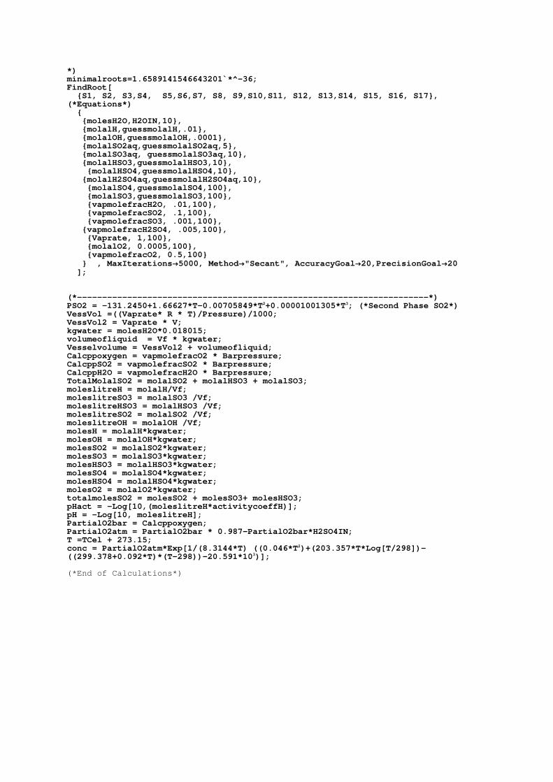
*) minimalroots=1.6589141546643201`*^-36; FindRoot[ {S1, S2, S3,S4, S5,S6,S7, S8, S9,S10,S11, S12, S13,S14, S15, S16, S17}, (*Equations*) { {molesH2O,H2OIN,10}, {molalH,guessmolalH,.01}, {molalOH,guessmolalOH,.0001}, {molalSO2aq,guessmolalSO2aq,5}, {molalSO3aq, guessmolalSO3aq,10}, {molalHSO3,guessmolalHSO3,10}, {molalHSO4,guessmolalHSO4,10}, {molalH2SO4aq,guessmolalH2SO4aq,10}, {molalSO4,guessmolalSO4,100}, {molalSO3,guessmolalSO3,100}, {vapmolefracH2O, .01,100}, {vapmolefracSO2, .1,100}, {vapmolefracSO3, .001,100}, {vapmolefracH2SO4, .005,100}, {Vaprate, 1,100}, {molalO2, 0.0005,100}, {vapmolefracO2, 0.5,100} } , MaxIterations→5000, Method→"Secant", AccuracyGoal→20,PrecisionGoal→20 ]; (*----------------------------------------------------------------------*) PSO2 = -131.2450+1.66627*T-0.00705849*T2+0.00001001305*T3; (*Second Phase SO2*) VessVol =((Vaprate* R * T)/Pressure)/1000; VessVol2 = Vaprate * V; kgwater = molesH2O*0.018015; volumeofliquid = Vf * kgwater; Vesselvolume = VessVol2 + volumeofliquid; Calcppoxygen = vapmolefracO2 * Barpressure; CalcppSO2 = vapmolefracSO2 * Barpressure; CalcppH2O = vapmolefracH2O * Barpressure; TotalMolalSO2 = molalSO2 + molalHSO3 + molalSO3; moleslitreH = molalH/Vf; moleslitreSO3 = molalSO3 /Vf; moleslitreHSO3 = molalHSO3 /Vf; moleslitreSO2 = molalSO2 /Vf; moleslitreOH = molalOH /Vf; molesH = molalH*kgwater; molesOH = molalOH*kgwater; molesSO2 = molalSO2*kgwater; molesSO3 = molalSO3*kgwater; molesHSO3 = molalHSO3*kgwater; molesSO4 = molalSO4*kgwater; molesHSO4 = molalHSO4*kgwater; molesO2 = molalO2*kgwater; totalmolesSO2 = molesSO2 + molesSO3+ molesHSO3; pHact = -Log[10,(moleslitreH*activitycoeffH)]; pH = -Log[10, moleslitreH]; PartialO2bar = Calcppoxygen; PartialO2atm = PartialO2bar * 0.987-PartialO2bar*H2SO4IN; T =TCel + 273.15; conc = PartialO2atm*Exp[1/(8.3144*T) ((0.046*T2)+(203.357*T*Log[T/298])-((299.378+0.092*T)*(T-298))-20.591*103)]; (*End of Calculations*)

Appendix E.

Macros in Visual Basic

Example to generate a continuous buffered sample clocked digital pulse train

from a Counter Output Channel.

Public Class MainForm

Inherits System.Windows.Forms.Form

Private idleState As COPulseIdleState

Private WithEvents dutyCycleMaxTextBox As System.Windows.Forms.TextBox

Private WithEvents channelParameterGroupBox As

System.Windows.Forms.GroupBox

Private WithEvents counterComboBox As System.Windows.Forms.ComboBox

Private WithEvents idleStateGroupBox As System.Windows.Forms.GroupBox

Private WithEvents highRadioButton As System.Windows.Forms.RadioButton

Private WithEvents lowRadioButton As System.Windows.Forms.RadioButton

Private WithEvents physicalChannelLabel As System.Windows.Forms.Label

Friend WithEvents clockSourceLabel As System.Windows.Forms.Label

Private WithEvents dutyCycleMaxLabel As System.Windows.Forms.Label

Private WithEvents dutyCycleMinTextBox As System.Windows.Forms.TextBox

Private WithEvents frequencyTextBox As System.Windows.Forms.TextBox

Private WithEvents frequencyLabel As System.Windows.Forms.Label

Private WithEvents pwmParametersGroupBox As


Private WithEvents dutyCycleMinLabel As System.Windows.Forms.Label

Private WithEvents timingParametersGroupBox As


Friend WithEvents clockSourceTextBox As System.Windows.Forms.TextBox

Friend WithEvents rateLabel As System.Windows.Forms.Label

Friend WithEvents samplesLabel As System.Windows.Forms.Label

Friend WithEvents samplesPerChannelNumeric As

System.Windows.Forms.NumericUpDown

Friend WithEvents rateNumeric As System.Windows.Forms.NumericUpDown

Private WithEvents stopButton As System.Windows.Forms.Button

Private WithEvents startButton As System.Windows.Forms.Button

Private myTask As Task

#Region " Windows Form Designer generated code "

Public Sub New()

MyBase.New()

Application.EnableVisualStyles()

'This call is required by the Windows Form Designer.

InitializeComponent()

'Add any initialization after the InitializeComponent() call

idleState = COPulseIdleState.Low

counterComboBox.Items.AddRange(DaqSystem.Local.GetPhysicalChannels(PhysicalC

hannelTypes.CO, PhysicalChannelAccess.External))

If (counterComboBox.Items.Count > 0) Then

counterComboBox.SelectedIndex = 0

End If

End Sub

'Form overrides dispose to clean up the component list.

Protected Overloads Overrides Sub Dispose(ByVal disposing As Boolean)

If disposing Then

If Not (components Is Nothing) Then

components.Dispose()

End If

End If

MyBase.Dispose(disposing)

End Sub

'Required by the Windows Form Designer

Private components As System.ComponentModel.IContainer

'NOTE: The following procedure is required by the Windows Form Designer

'It can be modified using the Windows Form Designer.

'Do not modify it using the code editor.

<System.Diagnostics.DebuggerStepThrough()> Private Sub

InitializeComponent()

Dim resources As System.ComponentModel.ComponentResourceManager =

New System.ComponentModel.ComponentResourceManager(GetType(MainForm))

Me.dutyCycleMaxTextBox = New System.Windows.Forms.TextBox

Me.channelParameterGroupBox = New System.Windows.Forms.GroupBox

Me.counterComboBox = New System.Windows.Forms.ComboBox

Me.idleStateGroupBox = New System.Windows.Forms.GroupBox

Me.highRadioButton = New System.Windows.Forms.RadioButton

Me.lowRadioButton = New System.Windows.Forms.RadioButton

Me.physicalChannelLabel = New System.Windows.Forms.Label

Me.clockSourceLabel = New System.Windows.Forms.Label

Me.dutyCycleMaxLabel = New System.Windows.Forms.Label

Me.dutyCycleMinTextBox = New System.Windows.Forms.TextBox

Me.frequencyTextBox = New System.Windows.Forms.TextBox

Me.frequencyLabel = New System.Windows.Forms.Label

Me.pwmParametersGroupBox = New System.Windows.Forms.GroupBox

Me.dutyCycleMinLabel = New System.Windows.Forms.Label

Me.timingParametersGroupBox = New System.Windows.Forms.GroupBox

Me.clockSourceTextBox = New System.Windows.Forms.TextBox

Me.rateLabel = New System.Windows.Forms.Label

Me.samplesLabel = New System.Windows.Forms.Label

Me.samplesPerChannelNumeric = New System.Windows.Forms.NumericUpDown

Me.rateNumeric = New System.Windows.Forms.NumericUpDown

Me.stopButton = New System.Windows.Forms.Button

Me.startButton = New System.Windows.Forms.Button

Me.channelParameterGroupBox.SuspendLayout()

Me.idleStateGroupBox.SuspendLayout()

Me.pwmParametersGroupBox.SuspendLayout()

Me.timingParametersGroupBox.SuspendLayout()

CType(Me.samplesPerChannelNumeric,

System.ComponentModel.ISupportInitialize).BeginInit()

CType(Me.rateNumeric,

System.ComponentModel.ISupportInitialize).BeginInit()

Me.SuspendLayout()

'

'dutyCycleMaxTextBox

'

Me.dutyCycleMaxTextBox.Location = New System.Drawing.Point(112, 82)

Me.dutyCycleMaxTextBox.Name = "dutyCycleMaxTextBox"

Me.dutyCycleMaxTextBox.Size = New System.Drawing.Size(132, 20)

Me.dutyCycleMaxTextBox.TabIndex = 11

Me.dutyCycleMaxTextBox.Text = "0.8"

'

'channelParameterGroupBox

'

Me.channelParameterGroupBox.Controls.Add(Me.counterComboBox)

Me.channelParameterGroupBox.Controls.Add(Me.idleStateGroupBox)

Me.channelParameterGroupBox.Controls.Add(Me.physicalChannelLabel)

Me.channelParameterGroupBox.FlatStyle =

System.Windows.Forms.FlatStyle.System

Me.channelParameterGroupBox.Location = New System.Drawing.Point(10,

9)

Me.channelParameterGroupBox.Name = "channelParameterGroupBox"

Me.channelParameterGroupBox.Size = New System.Drawing.Size(250, 117)

Me.channelParameterGroupBox.TabIndex = 7

Me.channelParameterGroupBox.TabStop = False

Me.channelParameterGroupBox.Text = "Channel Parameters:"

'

'counterComboBox

'

Me.counterComboBox.Location = New System.Drawing.Point(112, 16)

Me.counterComboBox.Name = "counterComboBox"

Me.counterComboBox.Size = New System.Drawing.Size(132, 21)

Me.counterComboBox.TabIndex = 1

Me.counterComboBox.Text = "Dev1/ctr0"

'

'idleStateGroupBox

'

Me.idleStateGroupBox.Controls.Add(Me.highRadioButton)

Me.idleStateGroupBox.Controls.Add(Me.lowRadioButton)

Me.idleStateGroupBox.FlatStyle =


Me.idleStateGroupBox.Location = New System.Drawing.Point(6, 43)

Me.idleStateGroupBox.Name = "idleStateGroupBox"

Me.idleStateGroupBox.Size = New System.Drawing.Size(238, 64)

Me.idleStateGroupBox.TabIndex = 6

Me.idleStateGroupBox.TabStop = False

Me.idleStateGroupBox.Text = "Idle State:"

'

'highRadioButton

'

Me.highRadioButton.FlatStyle = System.Windows.Forms.FlatStyle.System

Me.highRadioButton.Location = New System.Drawing.Point(123, 24)

Me.highRadioButton.Name = "highRadioButton"

Me.highRadioButton.Size = New System.Drawing.Size(64, 24)

Me.highRadioButton.TabIndex = 1

Me.highRadioButton.Text = "High"

'

'lowRadioButton

'

Me.lowRadioButton.Checked = True

Me.lowRadioButton.FlatStyle = System.Windows.Forms.FlatStyle.System

Me.lowRadioButton.Location = New System.Drawing.Point(51, 24)

Me.lowRadioButton.Name = "lowRadioButton"

Me.lowRadioButton.Size = New System.Drawing.Size(64, 24)

Me.lowRadioButton.TabIndex = 0

Me.lowRadioButton.TabStop = True

Me.lowRadioButton.Text = "Low"

'

'physicalChannelLabel

'

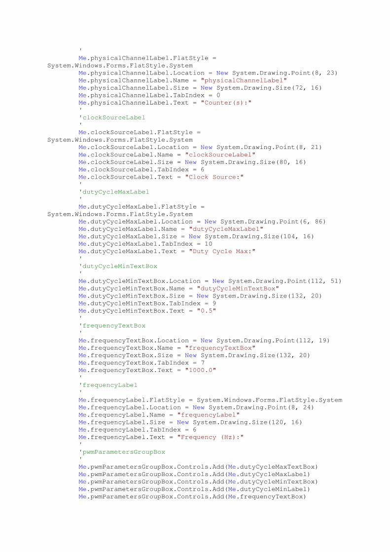
Me.physicalChannelLabel.FlatStyle =


Me.physicalChannelLabel.Location = New System.Drawing.Point(8, 23)

Me.physicalChannelLabel.Name = "physicalChannelLabel"

Me.physicalChannelLabel.Size = New System.Drawing.Size(72, 16)

Me.physicalChannelLabel.TabIndex = 0

Me.physicalChannelLabel.Text = "Counter(s):"

'

'clockSourceLabel

'

Me.clockSourceLabel.FlatStyle =


Me.clockSourceLabel.Location = New System.Drawing.Point(8, 21)

Me.clockSourceLabel.Name = "clockSourceLabel"

Me.clockSourceLabel.Size = New System.Drawing.Size(80, 16)

Me.clockSourceLabel.TabIndex = 6

Me.clockSourceLabel.Text = "Clock Source:"

'

'dutyCycleMaxLabel

'

Me.dutyCycleMaxLabel.FlatStyle =


Me.dutyCycleMaxLabel.Location = New System.Drawing.Point(6, 86)

Me.dutyCycleMaxLabel.Name = "dutyCycleMaxLabel"

Me.dutyCycleMaxLabel.Size = New System.Drawing.Size(104, 16)

Me.dutyCycleMaxLabel.TabIndex = 10

Me.dutyCycleMaxLabel.Text = "Duty Cycle Max:"

'

'dutyCycleMinTextBox

'

Me.dutyCycleMinTextBox.Location = New System.Drawing.Point(112, 51)

Me.dutyCycleMinTextBox.Name = "dutyCycleMinTextBox"

Me.dutyCycleMinTextBox.Size = New System.Drawing.Size(132, 20)

Me.dutyCycleMinTextBox.TabIndex = 9

Me.dutyCycleMinTextBox.Text = "0.5"

'

'frequencyTextBox

'

Me.frequencyTextBox.Location = New System.Drawing.Point(112, 19)

Me.frequencyTextBox.Name = "frequencyTextBox"

Me.frequencyTextBox.Size = New System.Drawing.Size(132, 20)

Me.frequencyTextBox.TabIndex = 7

Me.frequencyTextBox.Text = "1000.0"

'

'frequencyLabel

'

Me.frequencyLabel.FlatStyle = System.Windows.Forms.FlatStyle.System

Me.frequencyLabel.Location = New System.Drawing.Point(8, 24)

Me.frequencyLabel.Name = "frequencyLabel"

Me.frequencyLabel.Size = New System.Drawing.Size(120, 16)

Me.frequencyLabel.TabIndex = 6

Me.frequencyLabel.Text = "Frequency (Hz):"

'

'pwmParametersGroupBox

'

Me.pwmParametersGroupBox.Controls.Add(Me.dutyCycleMaxTextBox)

Me.pwmParametersGroupBox.Controls.Add(Me.dutyCycleMaxLabel)

Me.pwmParametersGroupBox.Controls.Add(Me.dutyCycleMinTextBox)

Me.pwmParametersGroupBox.Controls.Add(Me.dutyCycleMinLabel)

Me.pwmParametersGroupBox.Controls.Add(Me.frequencyTextBox)

Me.pwmParametersGroupBox.Controls.Add(Me.frequencyLabel)

Me.pwmParametersGroupBox.Location = New System.Drawing.Point(10,

252)

Me.pwmParametersGroupBox.Name = "pwmParametersGroupBox"

Me.pwmParametersGroupBox.Size = New System.Drawing.Size(250, 110)

Me.pwmParametersGroupBox.TabIndex = 9

Me.pwmParametersGroupBox.TabStop = False

Me.pwmParametersGroupBox.Text = "Pulse-width Modulation Parameters:"

'

'dutyCycleMinLabel

'

Me.dutyCycleMinLabel.FlatStyle =


Me.dutyCycleMinLabel.Location = New System.Drawing.Point(8, 55)

Me.dutyCycleMinLabel.Name = "dutyCycleMinLabel"

Me.dutyCycleMinLabel.Size = New System.Drawing.Size(104, 16)

Me.dutyCycleMinLabel.TabIndex = 8

Me.dutyCycleMinLabel.Text = "Duty Cycle Min:"

'

'timingParametersGroupBox

'

Me.timingParametersGroupBox.Controls.Add(Me.clockSourceLabel)

Me.timingParametersGroupBox.Controls.Add(Me.clockSourceTextBox)

Me.timingParametersGroupBox.Controls.Add(Me.rateLabel)

Me.timingParametersGroupBox.Controls.Add(Me.samplesLabel)

Me.timingParametersGroupBox.Controls.Add(Me.samplesPerChannelNumeric)

Me.timingParametersGroupBox.Controls.Add(Me.rateNumeric)

Me.timingParametersGroupBox.Location = New System.Drawing.Point(10,

132)

Me.timingParametersGroupBox.Name = "timingParametersGroupBox"

Me.timingParametersGroupBox.Size = New System.Drawing.Size(250, 114)

Me.timingParametersGroupBox.TabIndex = 8

Me.timingParametersGroupBox.TabStop = False

Me.timingParametersGroupBox.Text = "Timing Parameters:"

'

'clockSourceTextBox

'

Me.clockSourceTextBox.Location = New System.Drawing.Point(112, 19)

Me.clockSourceTextBox.Name = "clockSourceTextBox"

Me.clockSourceTextBox.Size = New System.Drawing.Size(132, 20)

Me.clockSourceTextBox.TabIndex = 7

Me.clockSourceTextBox.Text = "/Dev1/PFI7"

'

'rateLabel

'

Me.rateLabel.FlatStyle = System.Windows.Forms.FlatStyle.System

Me.rateLabel.Location = New System.Drawing.Point(8, 85)

Me.rateLabel.Name = "rateLabel"

Me.rateLabel.Size = New System.Drawing.Size(64, 16)

Me.rateLabel.TabIndex = 10

Me.rateLabel.Text = "Rate (Hz):"

'

'samplesLabel

'

Me.samplesLabel.FlatStyle = System.Windows.Forms.FlatStyle.System

Me.samplesLabel.Location = New System.Drawing.Point(8, 53)

Me.samplesLabel.Name = "samplesLabel"

Me.samplesLabel.Size = New System.Drawing.Size(104, 16)

Me.samplesLabel.TabIndex = 8

Me.samplesLabel.Text = "Samples / Channel:"

'

'samplesPerChannelNumeric

'

Me.samplesPerChannelNumeric.Location = New System.Drawing.Point(112,

51)

Me.samplesPerChannelNumeric.Maximum = New Decimal(New Integer()

{1000000, 0, 0, 0})

Me.samplesPerChannelNumeric.Name = "samplesPerChannelNumeric"

Me.samplesPerChannelNumeric.Size = New System.Drawing.Size(132, 20)

Me.samplesPerChannelNumeric.TabIndex = 9

Me.samplesPerChannelNumeric.Value = New Decimal(New Integer() {1000,

0, 0, 0})

'

'rateNumeric

'

Me.rateNumeric.DecimalPlaces = 2

Me.rateNumeric.Location = New System.Drawing.Point(112, 83)

Me.rateNumeric.Maximum = New Decimal(New Integer() {1000000, 0, 0,

0})

Me.rateNumeric.Name = "rateNumeric"

Me.rateNumeric.Size = New System.Drawing.Size(132, 20)

Me.rateNumeric.TabIndex = 11

Me.rateNumeric.Value = New Decimal(New Integer() {100, 0, 0, 0})

'

'stopButton

'

Me.stopButton.Enabled = False

Me.stopButton.FlatStyle = System.Windows.Forms.FlatStyle.System

Me.stopButton.Location = New System.Drawing.Point(266, 56)

Me.stopButton.Name = "stopButton"

Me.stopButton.Size = New System.Drawing.Size(96, 32)

Me.stopButton.TabIndex = 6

Me.stopButton.Text = "Stop"

'

'startButton

'

Me.startButton.FlatStyle = System.Windows.Forms.FlatStyle.System

Me.startButton.Location = New System.Drawing.Point(266, 18)

Me.startButton.Name = "startButton"

Me.startButton.Size = New System.Drawing.Size(96, 32)

Me.startButton.TabIndex = 5

Me.startButton.Text = "Start"

'

'MainForm

'

Me.AutoScaleBaseSize = New System.Drawing.Size(5, 13)

Me.ClientSize = New System.Drawing.Size(372, 370)

Me.Controls.Add(Me.channelParameterGroupBox)

Me.Controls.Add(Me.pwmParametersGroupBox)

Me.Controls.Add(Me.timingParametersGroupBox)

Me.Controls.Add(Me.stopButton)

Me.Controls.Add(Me.startButton)

Me.FormBorderStyle =

System.Windows.Forms.FormBorderStyle.FixedDialog

Me.Icon = CType(resources.GetObject("$this.Icon"),

System.Drawing.Icon)

Me.MaximizeBox = False

Me.Name = "MainForm"

Me.StartPosition =

System.Windows.Forms.FormStartPosition.CenterScreen

Me.Text = "Digital Pulse Train - Continuous - Buffered"

Me.channelParameterGroupBox.ResumeLayout(False)

Me.idleStateGroupBox.ResumeLayout(False)

Me.pwmParametersGroupBox.ResumeLayout(False)

Me.pwmParametersGroupBox.PerformLayout()

Me.timingParametersGroupBox.ResumeLayout(False)

Me.timingParametersGroupBox.PerformLayout()

CType(Me.samplesPerChannelNumeric,

System.ComponentModel.ISupportInitialize).EndInit()

CType(Me.rateNumeric,

System.ComponentModel.ISupportInitialize).EndInit()

Me.ResumeLayout(False)

End Sub

#End Region

Private Sub startButton_Click(ByVal sender As System.Object, ByVal e As

System.EventArgs) Handles startButton.Click

Dim samplesPerChannel As Integer =

Convert.ToInt32(samplesPerChannelNumeric.Value)

Dim rate As Double = Convert.ToDouble(rateNumeric.Value)

Dim frequency As Double = Convert.ToDouble(frequencyTextBox.Text)

Dim dutyCycleMin As Double =

Convert.ToDouble(dutyCycleMinTextBox.Text)

Dim dutyCycleMax As Double =

Convert.ToDouble(dutyCycleMaxTextBox.Text)

Dim dutyStep As Double = (dutyCycleMax - dutyCycleMin) /

samplesPerChannel

Try

Dim data(samplesPerChannel - 1) As CODataFrequency

For I As Integer = 0 To data.Length - 1

data(I) = New CODataFrequency(frequency, dutyCycleMin +

dutyStep * I)

Next

myTask = New Task()

myTask.COChannels.CreatePulseChannelFrequency(counterComboBox.Text, _

"ContinuousPulseTrain", COPulseFrequencyUnits.Hertz,

idleState, 0.0, _

frequency, _

dutyCycleMin)

myTask.Timing.ConfigureSampleClock(clockSourceTextBox.Text,

rate, _

SampleClockActiveEdge.Rising,

SampleQuantityMode.ContinuousSamples)

Dim writer As CounterSingleChannelWriter = New

CounterSingleChannelWriter(myTask.Stream)

writer.WriteMultiSample(False, data)

AddHandler myTask.Done, AddressOf OnTaskDone

myTask.Start()

startButton.Enabled = False

stopButton.Enabled = True

Catch ex As DaqException

MessageBox.Show(ex.Message)

myTask.Dispose()

startButton.Enabled = True

stopButton.Enabled = False

End Try

End Sub

Private Sub stopButton_Click(ByVal sender As System.Object, ByVal e As

System.EventArgs) Handles stopButton.Click

myTask.Stop()

myTask.Dispose()



End Sub

Private Sub lowRadioButton_CheckedChanged(ByVal sender As Object, ByVal

e As System.EventArgs) Handles lowRadioButton.CheckedChanged

idleState = COPulseIdleState.Low

End Sub

Private Sub highRadioButton_CheckedChanged(ByVal sender As Object, ByVal

e As System.EventArgs) Handles highRadioButton.CheckedChanged

idleState = COPulseIdleState.High

End Sub

Private Sub OnTaskDone(ByVal sender As Object, ByVal e As

TaskDoneEventArgs)

Try



e.CheckForException()

myTask.Stop()

myTask.Dispose()

myTask = Nothing

Catch ex As Exception

MessageBox.Show(ex.Message)

myTask.Stop()

myTask.Dispose()

myTask = Nothing

End Try

End Sub

End Class

Appendix F.

Publications

In progress April 2013 to date: Ternary model with preliminary ternary and quaternary data using Mathematica.

M.Romero, R.Elder, R.W.K.Allen. Date to publish approximately: September 2013.

Conference Proceeding Low temperature SO2-O2-H2O VLE in the sulphur family of thermochemical cycles

M.Romero, R. Allen, R. Elder

01/2011; In proceeding of: International Conference on Hydrogen Production 2011, At Thessaloniki, Greece

ABSTRACT

Thermochemical cycles have great potential for massive scale, carbon-neutral hydrogen production. Of

particular interest are the Sulphur Iodine (SI) and the Hybrid Sulphur (HyS) cycles, both having a

common step consisting on the high temperature thermal decomposition of H2SO4. The energy

requirements are large and there is no known thermodynamic data for this particular system. In order

for a design-based approach to be taken for the low temperature separation, accurate vapour-liquid

equilibrium data is needed for the decomposition products: SO2-H2O-O2. This work experimentally

investigates both the binary SO2-H2O and ternary SO2-O2-H2O system at pressures up to 15 bar and

temperatures up to 80° C. Results are compared to a theoretical model based on weak electrolyte

thermodynamics. Good correlation between the model and experimental results is seen at low

pressures for the binary solution and across the pressure range for the ternary solution. The divergence

at high pressures in the binary comparison is thought to be due to the formation of two liquid phases,

and the underestimation of the dissolved SO2 salting-out effect. Online spectroscopic measurements

are being developed to measure this phenomenon.

Conference Proceeding Low Temperature Separations in the Sulphuric Acid Decomposition Stage of the Sulphur Iodine and Hybrid Sulphur Thermochemical Water Splitting Cycles

M. Romero R.H. Elder A. Shaw N. Elbakhbakhi G.H. Priestman R.W.K. Allen Detlef Stolten

(Hrsg.) Thomas Grube (Hrsg.)

01/2010; In proceeding of: 18th World Hydrogen Energy Conference 2010 - WHEC 2010, At Essen, Germany

ABSTRACT

The Sulphur Iodine and Hybrid Sulphur thermochemical cycles are promising routes for large scale

production of hydrogen from water. The thermal decomposition of aqueous sulphuric acid to form SO2,

O2 and H2O is common to both cycles and involves high temperatures and difficult separations. The

energy requirement is large due to the excess of water present. This work investigates the separations

involved with a view to improving efficiency.

Conference Proceeding Simultaneous Solubilities of Oxygen and Sulphur Dioxide in Water: Thermodynamic Data for the Sulphur Family of Thermochemical Cycles

M. Romero, R. Elder, A. Shaw, R. Allen

01/2010; In proceeding of: 2010 AIChE Annual Meeting, At Salt Lake City, US

ABSTRACT

The Sulphur family of thermochemical cycles shows great promise for the massive scale production of

hydrogen from water. The decomposition of sulphuric acid is a common stage in the cycles and poses

design problems due to the corrosive nature of the solution, the high temperatures involved and the

difficult separations required. The work considered here focuses on the oxygen separation stage of the

process where, in order for a science based design approach to be taken, thermodynamic data are

required for multicomponent phase equilibrium relationships between water, sulphur dioxide and

oxygen; H2O-SO2-O2. A bespoke vapour-liquid-equilibrium still is used to measure the simultaneous

solubilities of the ternary solution. The results are presented, along with a comparison to a model based

on weak electrolyte thermodynamics. The model can be used for flash calculations, necessary for the

design of the separation equipment.

Journal Article Measurements of the solubility of sulphur dioxide in water for the sulphur family of thermochemical cycles

Moises A. Romero, Andrew C. Shaw, Rachael H. Elder, Bruce C.R. Ewan, Ray W.K. Allen

International Journal of Hydrogen Energy (impact factor: 4.05). 01/2010; 38:4749.

ABSTRACT

In recent years, the Hybrid Sulphur (HyS) and Sulphur Iodine (SI) cycles have emerged as promising

routes for the massive scale thermochemical production of Hydrogen from water. Common to these

two cycles is a high temperature stage involving the decomposition of sulphuric acid to sulphur dioxide,

water and oxygen. The work considered here focuses on the oxygen separation stage of the process

where, in order for a science based design approach to be taken, thermodynamic data are required for

multicomponent phase equilibrium relationships between the decomposition products; H2O–SO2–O2.

A method of making flash calculations, useful in the separation equipment design, has been proposed

and coded into Mathematica®. Further, a vapour–liquid equilibrium still has been designed and built to

make measurements of the multicomponent solubility of sulphur dioxide and oxygen in water. The

experiments presented here concentrate on the binary SO2–H2O system, covering a wider range of

pressures than that found in the literature. Solubility, expressed in molality, was obtained at 25 and 40

°C and pressures ranging from 0.2 to 3.6 atm. Good agreement is seen between the experimental data

and the model at lower pressures, however improvements are needed at higher pressure. Preliminary

data for the ternary system at 40 °C is presented, showing good agreement with the multicomponent

model. Future work will focus on the three component system.

Appendix G.

Technical Drawings

1

1

2

2

3

3

4

4

5

5

6

6

A A

B B

C C

D D

DRAWNM.RomeroCHECKEDMRQA

MFG

APPROVEDMR

MR

22/05/2013University of Sheffield

TITLE

Mark IV Experiment Layout

SIZE

A3SCALE

DWG NO

Final Reactor Thesis 2013REV

1

SHEET 1 OF 1

A

B

C

D

E

F

G

H

I

J

Mark IV Laboratory SetupThe following diagram represents the laboratory setup used for the Mark IV experiments that were performed during this project A Reactor Thermocouple B Waterbath ThermocoupleC Bath ControllerD Mark IV ReactorE Heating Media Chemical & Biological EngineeringUniversity of Sheffield

F Fume cupboardG NI DAQ InterfaceH LabVIEW PCI Sulphur Dioxide and OxygenJ FTIR Spectrometer

1

1

2

2

3

3

4

4

5

5

6

6

A A

B B

C C

D D

DRAWNDr. M. RomeroCHECKEDMRQA

MFG

APPROVEDRWKA

MR

23/05/2013

23/05/2013

23/05/2013

23/05/2013

University of Sheffield

TITLE

Mark IV VLE Reactor

SIZE

A3SCALE

DWG NO

Mark IV VLE ReactorREV

1

SHEET 1 OF 1

A - GAS LIDB - OUTER PTFE GASKETC - SIGHT GLASSD - INNER PTFE GASKETE - REACTOR BODYF - BSP THREADG - VALVE HOLDERH - PLUG HOLES

I - GAS VALVEJ - LIQUID VALVEK - SLOTTED PTFE GASKETL - THERMOCOUPLE INSERTM - ATR GERMANIUM PRISMN - PTFE GERMANIUM SEATO - 45° FIBER OPTIC INSERTSP - LIQUID LID

Q - GAS CHAMBERR - VALVE SEATS - MULTIPHASE AREAT - ALIGNMENT PIN

Mark IV VLE Reactor

A

BC

D

E

F

G

H I

J

K

L

M

N

O

P

Q

RS

T

Consolidated Reference List

ABAOUD, H. & STEEB, H. 1998. The German-Saudi HYSOLAR program. International Journal of Hydrogen Energy, 23, 445-449.

BASS, M., DECUSATIS, C., ENOCH, J., LAKSHMINARAYANAN, V., LI, G., MACDONALD, C., MAHAJAN, V. & VAN STRYLAND, E. 2009. Handbook of Optics, Third Edition Volume I: Geometrical and Physical Optics, Polarized Light, Components and Instruments(set), McGraw-Hill Companies,Incorporated.


CARROLL, J. J. 1991. What is Henry's Law? Chemical Engineering Progress, 87, 48-52.



CRYSTRAN. 2012. Optical Properties of Materials [Online]. Available: http://www.crystran.co.uk/materials-data.htm.

DAUBERT, T. E. 1985. Chemical engineering thermodynamics, McGraw-Hill.

DREWNOWSKI, A. & SPECTER, S. 2004. Poverty and obesity: the role of energy density and energy costs. The American Journal of Clinical Nutrition, 79, 6-16.

DROLET, B., GRETZ, J., KLUYSKENS, D., SANDMANN, F. & WURSTER, R. 1996. The euro-québec hydro-hydrogen pilot project [EQHHPP]: demonstration phase. International Journal of Hydrogen Energy, 21, 305-316.

DUDLEY, B. 2012. BP statistical review of world energy.

DUNN, S. 2002. Hydrogen futures: toward a sustainable energy system. International Journal of Hydrogen Energy, 27, 235-264.

EHA. 2012. EHA March Newsletter [Online]. Available: http://www.h2euro.org/category/publications/newsletters/newsletters-2012/eha-newsletter-march-2012.


ELDER, R. H., SHAW, A., ROMERO, M., ELBAKHBAKHI, N., PRIESTMAN, G. H. & ALLEN, R. W. K. 2010. Low Temperature Separations in the Sulphuric Acid Decomposition Stage of the Sulphur Iodine and Hybrid Sulphur Thermochemical Water Splitting Cycles. In: DETLEF STOLTEN, T. G. E. F. J. G. (ed.) WHEC 2010. Essen, Germany: Forschungszentrum Jülich GmbH, Zentralbibliothek, Verlag.


GOLTSOV, V. A. & VEZIROGLU, T. N. 2001. From hydrogen economy to hydrogen civilization. International Journal of Hydrogen Energy, 26, 909-915.

GUBBINS, K. & WALKER, R. 1965. The Solubility and Diffusivity of Oxygen in Electrolytic Solutions. Journal of the Electrochemical Society, 112, 469.

HARVEY, K. B., MCCOURT, F. R. & SHURVELL, H. F. 1964. INFRARED ABSORPTION OF THE SO2 CLATHRATE-HYDRATE MOTION OF THE SO2 MOLECULE. Canadian Journal of Chemistry, 42, 960-963.


HIJIKATA, T. 2002. Research and development of international clean energy network using hydrogen energy (WE-NET). International Journal of Hydrogen Energy, 27, 115-129.

HIPPLER, M. & HAYNES, A. 2010. RE: Raman Spectroscopy Laboratory, Introduction. Type to M.ROMERO.

HIRSCH, R., BEZDEK, R. & WENDLING, R. Peaking of world oil production. Proceedings of the IV International Workshop on Oil and Gas Depletion, 2005. 19-20.

HUDSON, J. C. 1925. The solubility of sulphur dioxide in water and in aqueous solutions of potassium chloride and sodium sulphate. Journal of the Chemical Society, 127, 1332-1347.

J.JOOSTEN, P. G., A. KYDES, J.D.MAPLES 2008. The Impact of Increased Use of Hydrogen on Petroleum Consumption and Carbon Dioxide Emissions. 1 ed. Washington, D.C. U.S. 20585: Energy Information Administration, U.S.DOE.


JORGENSON, D. W. 1984. The Role of Energy in Productivity Growth. The American Economic Review, 74, 26-30.

KHAMIS, I. 2011. An overview of the IAEA HEEP software and international programmes on hydrogen production using nuclear energy. International Journal of Hydrogen Energy, 36, 4125-4129.

KRICHEVSKY, I. R. & KASARNOVSKY, J. S. 1935. Thermodynamical Calculations of Solubilities of Nitrogen and Hydrogen in Water at High Pressures. Journal of the American Chemical Society, 57, 2168-2171.



LIN, C.-T. & DAUBERT, T. E. 1978. Prediction of the Fugacity Coefficients of Nonpolar Hydrocarbon Systems from Equations of State. Industrial & Engineering Chemistry Process Design and Development, 17, 544-549.



MARTIN, L. R. & GOOD, T. W. 1991. Catalyzed oxidation of sulfur dioxide in solution: The iron-manganese synergism. Atmospheric Environment. Part A. General Topics, 25, 2395-2399.

MAURER, G. 1980. On the solubility of volatile weak electrolytes in aqueous solutions. Thermodynamics of aqueous systems with industrial applications; ACS Symposium Series, 133, 139-172.

MITSUGI, C., HARUMI, A. & KENZO, F. 1998. WE-NET: Japanese hydrogen program. International Journal of Hydrogen Energy, 23, 159-165.

MOHAMMADI, A. H. & RICHON, D. 2010. Equilibrium Data of Sulfur Dioxide and Methyl Mercaptan Clathrate Hydrates. Journal of Chemical & Engineering Data, 56, 1666-1668.

MOMIRLAN, M. & VEZIROGLU, T. N. 2002. Current status of hydrogen energy. Renewable and Sustainable Energy Reviews, 6, 141-179.

MORIARTY, P. & HONNERY, D. 2009. Hydrogen's role in an uncertain energy future. International Journal of Hydrogen Energy, 34, 31-39.


OTHMER, D. F., SILVIS, S. J. & SPIEL, A. 1952. Composition of Vapors from Boiling Binary Solutions: Pressure Equilibrium Still for Studying Water–Acetic Acid System. Industrial & Engineering Chemistry, 44, 1864-1872.

OUTOKUMPU 2002. Software: HSC chemistry version 5.0. Chemical Engineering Progress, 98, 28.

PASTOWSKI, A. & GRUBE, T. 2010. Scope and perspectives of industrial hydrogen production and infrastructure for fuel cell vehicles in North Rhine-Westphalia. Energy Policy, 38, 5382-5387.

PRAUSNITZ, J. M. 1969. Molecular Thermodynamics of Fluid-Phase Equilibria (Prentice-Hall International Series in the Physical and Chemical Engineering Sciences).

PRAUSNITZ, J. M., LICHTENTHALER, R. N. & DE AZEVEDO, E. G. 1986a. Molecular thermodynamics of fluid-phase equilibria, Prentice-Hall.

PRAUSNITZ, J. M., LICHTENTHALER, R. N. & DE AZEVEDO, E. G. 1986b. Molecular thermodynamics of fluid-phase equilibria. Prentice-Hall.

QUADRANT. 2011. Fluorosint® 207 Product Data Sheet [Online]. Available: http://www.quadrantplastics.com/fileadmin/quadrant/documents/QEPP/EU/Product_Data_Sheets_PDF/AEP/Fluorosint_207_E_PDS_2011.pdf.

RABE, A. E. & HARRIS, J. F. 1963. Vapor Liquid Equilibrium Data for the Binary System Sulfur Dioxide and Water. Journal of Chemical & Engineering Data, 8, 333-336.

REID, R. C., PRAUSNITZ, J. M. & POLING, B. E. 1987. The properties of gases and liquids, McGraw-Hill.

ROMERO, M. Low temperature SO2-O2-H2O VLE in the sulphur family of thermochemical cycles. In: ALLEN, R. W. K., ed. International Conference on Hydrogen Production, 2011 Thessaloniki, Greece. Hellas Research Centre, Greece.

RUMPF, B., WEYRICH, F. & MAURER, G. 1993. Simultaneous solubility of ammonia and sulfur dioxide in water at temperatures from 313.15 K to 373.15 K and pressures up to 2.2 MPa. Fluid Phase Equilibria, 83, 253-260.

SHAW, A. C. 2008a. The simultaneous solubility of sulphur dioxide and oxygen in water for the hybrid sulphur thermochemical cycle. Ph.D. Doctoral Thesis, University of Sheffield.

SHAW, A. C. 2008b. The simultaneous solubility of sulphur dioxide and oxygen in water for the hybrid sulphur thermochemical cycle. PhD Thesis, University of Sheffield.


SHERWOOD, T. K. 1925. Solubilities of Sulfur Dioxide and Ammonia in Water. Industrial & Engineering Chemistry, 17, 745-747.


STOLTEN, D. 2010. Hydrogen and Fuel Cells: Fundamentals, Technologies and Applications, John Wiley & Sons.

STUART, B. H. 2004. Infrared Spectroscopy: Fundamentals and Applications, John Wiley & Sons.

TAYLOR, M. 2006. Improvement of the Sulphur-Iodine cycle through the addition of ionic liquids. M.Phil, University of Sheffield.


TOWLER, G. & SINNOTT, R. K. 2007. Chemical Engineering Design: Principles, Practice and Economics of Plant and Process Design, Elsevier Science.

VAN BERKUM, J. G. & DIEPEN, G. A. M. 1979. Phase equilibria in SO2 + H2O: the sulfur dioxide gas hydrate, two liquid phases, and the gas phase in the temperature range 273 to 400 K and at pressures up to 400 MPa. The Journal of Chemical Thermodynamics, 11, 317-334.

VEZIROĞLU, T. N. & TAKAHASHI, P. K. Hydrogen energy progress VIII : proceedings of

the 8th World Hydrogen Energy Conference, Honolulu and Waikoloa, Hawaii, U.S.A., 22-27 July 1990. In: VEZIROĞLU, T. N. & TAKAHASHI, P. K., eds., 1990 New York :.

Pergamon Press.

WARN, J. R. W. & PETERS, A. P. H. 1996. Concise Chemical Thermodynamics, 2nd Edition, N. Thornes.

WESTON, K. C. 1992. Energy Conversion, West Publishing Company.

ZEMAITIS, J. F., CLARK, D. M., RAFAL, M. & SCRIVINER, N. C. 1986. Handbook of Aqueous Electrolyte Thermodynamics, New York, AIChE

Low temperature studies for the sulphuric acid decomposition ...

Documents

Transcript of Low temperature studies for the sulphuric acid decomposition ...