arX

iv:a

stro

-ph/

0309

258v

1 9

Sep

200

3

Submitted to AJ, June 2003

The morphological decomposition of Abell 8681

S.P.Driver

The Research School of Astronomy and Astrophysics, The Australian National University,

Weston Creek, ACT 2611, AUSTRALIA

spd@mso.anu.edu.au

S.C.Odewahn, L.Echevarria, S.H.Cohen, R.A.Windhorst

School of Physics and Astronomy, Arizona State University, Tempe, AZ 85287-1504, USA

S.Phillipps

Department of Physics, University of Bristol, Bristol, BS8 1TL, UK

and

W.J.Couch

School of Physics and Astronomy, University of New South Wales, Sydney, NSW 2052,

AUSTRALIA

ABSTRACT

We report on the morphological luminosity functions (LFs) and radial profiles

derived for the galaxy population within the rich cluster Abell 868 (z = 0.153)

based purely on Hubble Space Telescope Imaging in F606W . We recover Schechter

functions (−24.0 < MF606W − 5logh0.65 < −16.0) within a 0.65h0.65 Mpc radius

for early(E/S0)-, mid(Sabc)- and late(Sd/Irr)- type galaxies of:

M∗All − 5 log10 h0.65 = −22.4+0.6

−0.6, αAll = −1.27+0.2−0.2

M∗E/S0 − 5 log10 h0.65 = −21.6+0.6

−0.6, αE/S0 = −0.5+0.2−0.3

M∗Sabc − 5 log10 h0.65 = −21.3+1.0

−0.9, αSabc = −1.2+0.2−0.2

M∗Sd/Irr − 5 log10 h0.65 = −17.4+0.7

−0.7, αSd/Irr = −1.4+0.6−0.5.

The early-, mid- and late- types are all consistent with the recent field morpho-

logical LFs based on recent analysis of the Sloan Digital Sky Survey — Early

– 2 –

Data Release (SDSS-EDR; Nakamura et al 2003). From a detailed error anal-

ysis, including clustering of the background population, we note that improved

statistics can only come from combining data from many clusters.

We also examine the luminosity-density and number-density profiles as a function

of morphology and draw the following conclusions: (1) The galaxies responsible

for the steep faint-end slope are predominantly of late-type morphology, (2) The

cluster core is dominated by elliptical galaxies, (3) The core is devoid of late-

types systems, (4) The luminosity-density as a function of morphological type

is skewed towards early-types when compared to the field, (5) Up to half of

the elliptical galaxies may have formed from the spiral population through core

disk-destruction process(es).

We believe the most plausible explanation is the conventional one that late-types

are destroyed during transit through the cluster core and that mid-types are

converted into early-types through a similar process, which destroys the outer

disk and results in a more tightly bound population of core ellipticals.

Subject headings: galaxies: luminosity function, mass function — galaxies: clus-

ters: general — galaxies: evolution — galaxies: formation galaxies: fundamental

parameters — galaxies: dwarf

1. Introduction

The overall luminosity distribution of galaxies in any environment is the traditional

tool for describing the galaxy population (see Binggeli, Sandage & Tammann 1988, BST).

However, while it categorises the number-density as a function of absolute magnitude it

provides no information on the morphology, structure, spectra or star-formation rates of the

contributing galaxies. While studies may show that the luminosity function (LF) of the field,

groups and rich clusters are comparable at bright magnitudes (see for example De Propris et

al 2003 and Christlein & Zabludoff 2003), this is by no means conclusive proof that the entire

galaxy population and characteristics are identical. Indeed the morphology-density (Dressler

1Based on observations made with the NASA/ESA Hubble Space Telescope, obtained at the Space

Telescope Science Institute, which is operated by the Association of Universities for Research in Astronomy,

Inc., under NASA contract NAS 5-26555. These observations are associated with program #8203.

– 3 –

1980; Dressler et al 1997) and the dwarf population-density (Phillipps et al 1998) relations

clearly tell us that local galaxy density is important and that luminous elliptical galaxies

prefer clustered environments and low luminosity irregular galaxies field environments. In

short, a single luminosity distribution may bypass exactly the information that is required

to decipher the subtleties of the environmental dependency of galaxy evolution.

In addition, recent measurements of the LFs in rich clusters have led to inconsistent

conclusions as to whether there is a universal LF (see for example Trentham 1998) or a

dwarf population-density relation (Phillipps et al 1998). In a study of 7 Abell clusters

Driver et al (1998a), using a statistical background subtraction method, found significant

variation in the faint-end slopes whereby low density clusters exhibit steeper slopes (or higher

dwarf-to-giant ratios). The same result was independently found for a separate sample of 35

clusters by Lopez-Cruz (1997)2. However, both methods rely on a statistical subtraction of

the background population which, although rigorously tested in Driver et al (1998b), has

been criticized by Valotto, Moore & Lambas (2001) as being susceptible to cosmic variance

along the line of sight — although, it is difficult to understand how cosmic variance can lead

to the relatively clean relation between luminosity and local density seen by Phillipps et al

(1998) and the smooth radial increase in dwarf-to-giant ratios seen in A2554 (Smith et al

2000) and A2218 (Pracy et al 2003). More recently Barkhouse & Yee (2003) report a general

trend of an increase in faint-end slope with cluster radius from α = −1.81 to α = −2.07

for a sample of 17 nearby clusters. For very local clusters where cluster membership can be

ascertained more easily, such as Virgo and Coma, Trentham & Tully (2002) summarise the

state-of play and argue for a universal LF (see also review by Driver & De Propris 2003

and references therein). Trentham & Hodgkin (2001) however argue the opposite noting

the significant difference in dwarf-to-giant ratio between Virgo and Ursa Major. Some part

of this confusion most likely comes about from the apparent different clustering of the two

dwarf populations. For example Sandage, Binggeli & Tammann (1985) found a generally

centrally concentrated distribution of dwarf ellipticals in Virgo, whereas Sabatini et al (2003)

report to the contrary a significant steepening in the luminosity function faint-end slope with

cluster-centric radius, also in Virgo, due to low surface brightness dwarf irregulars. In the

Coma cluster Thompson & Gregory (1993) identify three dwarf populations (dIs, dEs and

dSphs) each with distinct clustering signatures.

Taken together, the sparse information contained within a single LF and the contra-

dictions in the literature, it seems necessary to deconstruct the LF further, incorporating

morphological/structural and/or color information in the analysis. It is also worth noting

2It is worth noting that both studies used a fixed field-of-view size, limited by the respective detectors,

and hence representing progressively larger physical extents for higher redshift clusters.

– 4 –

that some component of the confusion may arise from radial dependencies and the specific

areal extent over which the cluster has been surveyed — particularly if the above radial

trends seen in Virgo are confirmed as universal. To this end we have embarked upon a

detailed observational program, including space-based optical and X-ray observations, and

ground-based narrow-band imaging, of the rich cluster A868. In this paper we focus purely

on the morphological aspects based upon a 12 orbit Wide Field Planetary Camera 2 mosaic

of the cluster A868. In particular we are interested in the suggestion that there may exist

a universal LF for each morphological type (BST) and that only the relative normalisation

changes with environment. Analysis of the two-degree field galaxy redshift survey by De Pro-

pris et al (2003) find that although the overall luminosity distribution is invariant between

the field and cluster composite, differences do arise when subdivided according to spectral

type. Christlein & Zabludoff (2003) confirm this result based on their independent spectral

study of the population in and around 6 low redshift clusters. These latter results, based

on spectral classifications, generally supports the developing notion that star-formation is

quenched in the infalling galaxy population (Lewis et al 2002, Gomez et al 2003, see

also review by Bower & Balogh 2003), unfortunately spectral classifications cannot address

whether the population has physically changed as well.

The cluster A868 itself, is unremarkable, except that it formed part of a cluster popu-

lation study by Driver et al (1998a), in which a high dwarf-to-giant ratio was found. The

primary purpose of these HST data were to study the morphologies and structural properties

of the giants and dwarfs, and in particular to identify the nature of the population responsible

for the apparently steep LF upturn at the faint-end. An initial attempt in this regard, using

ground-based data, was made by Boyce et al (2001). They concluded that the population

responsible for the faint upturn could be subdivided into three categories: a contaminating

population of background high-redshift ellipticals, an overdensity (relative to the giants) of

dwarf ellipticals, and an overdensity of dwarf irregulars. The type classification was made

on the basis of color. Boyce et al (2001) noted that when the population of contaminating

background galaxies was removed, the overall LF still showed a distinct upturn (α = −1.22)

and a generally high overdensity of dwarf galaxies. From the colors it was concluded that

the main component of this population was blue and therefore presumed to consist of dwarf

Irregular galaxies. Furthermore Boyce et al (2001) argued that the core was devoid of dIrrs

which were mostly destroyed via processes such as galaxy harassment (Moore, Lake & Katz

1998), thus accounting for the increase in the luminosity function faint-end slope from the

centre outwards (Driver et al 1998a).

The plan of this paper is as follows: In section 2 we summarise the observations, reduc-

tion and analysis of the Hubble Space Telescope images. In section 3 we describe and validate

the morphological classification process, and in section 4 we describe the appropriate error

– 5 –

analysis incorporating the clustering signature of the background population. In section 5

we show the overall and morphological luminosity distributions, determined via statistical

background subtraction, and compare them to recent field estimates to test BSTs hypothesis.

In section 6 we investigate the radial distribution in terms of the luminosity- and number-

density profile of each morphological type and conclude in section 7. We adopt Ho = 65

km/s/Mpc, ΩM = 0.3 and ΩΛ = 0.7 throughout, this results in a distance modulus to A868

of 39.47 mags (excluding K-correction).

2. Data Acquisition, Reduction and Analysis

A868 formed part of a cluster population study by Driver et al (1998a), in which a

high dwarf-to-giant ratio was found (see also Boyce et al 2001). To pursue this further

12 orbits were allocated in Cycle 8 with the Wide Field Planetary Camera 2 onboard the

Hubble Space Telescope (HST3) to obtain a six-pointing F606W mosaic of the cluster. A868

lies at coordinates αJ2000.0 = 09h45m26.43s, δJ2000.0 = −08o39′

06.7′′

, z = 0.153 (Strubble &

Rood 1999). The cluster has an Abell richness class 3, and is of Bautz-Morgan type II-III

(see Driver et al 1998a and Boyce et al 2001 for the earlier work on A868).

The data comprise 24 individual exposures of 1100s, each targeted at six individual

and marginally overlapping pointings (see Fig. 1). The data were combined using a pixel

clipping algorithm based on local sky statistics developed for use with WFPC2 images in

the lmorpho package (Odewahn et al 2002). Extensive tests were made comparing the

photometry derived from such stacks, to those derived from the drizzle algorithm (Fruchter

& Hook 2002) with no appreciable systematic difference found. The lmorpho stacks,

produced in a more straight-forward fashion, and free of problems associated with correlated

pixel noise, were adopted for further use. The final pixel scale is 0.0996 arcsec/pixel and

the full mosaic field covers an area of 0.007545 sq. degrees. Fig. 2 shows the WFPC2

chip containing the cluster core, showing the dominant cD and D galaxies, and evidence

for strong gravitational lensing. The photometric zeropoint for each mosaic was 30.443, as

taken from Holtzmann et al (1995), placing the photometry onto the Vega system. Initial

object source catalogs were derived with sextractor (Bertin & Arnouts 1996) using a 2σ

sky level threshold (per pixel) and a minimum isophotal area of 5 pixels. A gui-based

image editor in the lmorpho package was used to visually inspect image segmentation

over the field and edit obvious problems. Image postage stamps were prepared for each

3Based on observations made with the NASA/ESA Hubble Space Telescope. STScI is operated by the

Association of Universities for Research in Astronomy, Inc. under NASA contact NAS 5-26555.

– 6 –

detected source and the galphot package in lmorpho was used to perform automated

galaxy surface photometry. This package incorporates information about nearby cataloged

sources and performs modest corrections designed to decrease photometric degradation from

field crowding. The lmorpho catalog for 1616 valid objects in A868 contained a variety

of image structural parameters as well as total magnitudes and quartile radii (including the

effective radius) — for full details of the inner workings of this software package see Odewahn

et al (2002). Note that final magnitudes are extinction corrected using Schlegel, Finkbeiner

& Davis (1998) dust maps. Briefly an initial isophotal magnitude within an elliptical

aperture is measured and the data is corrected to total based upon the extrapolated profile

fit. In most cases this provides an excellent approximation to the total magnitude and is

ideal for crowded sight-lines such as A868. However its well known that for anomalous

and/or flat profile objects the isophotal correction can become unrealistically large. As a

check of the isophotal corrections we show the isophotal versus total magnitudes for the

full A868 galaxy population (see Fig. 3). Clearly a small fraction of objects do indeed have

unrealistic isophotal corrections. We hence adopt a cap to the isophotal correction shown

as the dotted line. This is a simple power-law fitted to the lower bound of the brighter data

(note that not surprisingly the cap is only required for the late-types, triangles on Fig. 4,

which exhibit non-standard profile shapes). The expression for the isophotal cap is given by:

mTotal ≤ mIso + 0.25 − 0.0055(mIso − 16)2.5

Finally Fig. 4 shows the apparent bivariate brightness distribution, this highlights that

stars and galaxies are well separated to mF606W ≤ 24.0 mag, and that the bulk of the galaxy

population lies above the surface brightness detection isophote to the same limit. From Fig.

4 it is also apparent that earlier-types are of higher effective surface brightness in line with

conventional wisdom.

2.1. Reference field counts

In order to determine the contribution to the A868 galaxy counts from the field, we

performed an identical reduction and analysis on the Hubble Deep Field North (HDFN),

Hubble Deep Field South (HDFS) and the deep field 53W002 (Driver et al 1995; Windhorst,

Keel & Pascarelle 1998) — all observed in F606W, covering ∼ 0.0011 sq deg, and calibrated

onto the same photometric system as A868 (see Cohen et al 2003 for further details of

these specific fields). However these three deep fields only provide reference counts at faint

magnitudes (mF606W > 21 mag). To provide reference counts at brighter magnitudes we

adopt the Millennium Galaxy Catalogue (MGC; Liske et al 2003; Cross et al 2003) and

convert the MGC photometry fromBMGC to F606W. This is achieved by convolving the Isaac

– 7 –

Newton Telescope’s KPNO B and the Hubble Space Telescope’s F606W filter+instrument

transmission functions with the mean zero redshift cosmic spectrum from the 2dF galaxy

redshift survey (Baldry et al 2002), after dividing out the equivalent flux calibrated spectrum

for Vega (see for example Sung & Bessell 2000). This resulted in a transformation of:

(BMGC −F606W )V ega = +1.06. Although the MGC counts extend to B = 24 mag, the color

transformation above will only be appropriate for non-cosmological distances, i.e., B ≤ 18.25

mag.

3. Galaxy Classification

Object classification for the A868, HDFN, HDFS, 53W002 fields were performed using

an Artificial Neural Network (ANN), as described in Odewahn et al (1996). Briefly, the

ANNs were initially trained on a sample classified by eye, drawn from a variety of datasets

including the HST BBpar (Cohen et al 2003) and RC3 catalogues (de Vaucouleurs et al

1995). The ANNs take as input parameters a set of structural measurements for each image

(seven isophotal areas and a seeing/PSF measurement) and output a classification onto the

16 step de Vaucouleurs’ t-type system (see de Vaucouleurs et al 1995) with an additional

step added for stars. Stars are defined as t-type=12, early-types (E/S0) as −6.0 ≤ t-type

≤ 0.0, mid-types (Sabc) as 0.0 < t-type ≤ 6.0, and late-types (Sd/Irr) as 6.0 < t-type

≤ 10.0. An error is allocated to each classification based upon the dispersion amongst five

independently trained ANNs. As a check of the classification accuracy we visually inspected

all objects brighter than mF606W < 24.0 mag. In 80 out of the 663 cases a visual override

was necessary. The majority of these were due to entangled isophotes (i.e., crowding) which

is known to cause some problems with ANN classifications. Table 1 sumarises the overrides

and no obvious classification bias is apparent. We also note that three of these errors were

the A868 central cD and two D galaxies which were all erroneously classified as Sabcs. As no

cD or D galaxies were included in the ANN training sets, it is understandable that the giant

bulge surrounded by a low surface brightness halo could readily be confused with a mid-type

spiral. Excluding these three specific objects, thereby gives an unchecked ANN classification

accuracy of ∼ 90 per cent. Postage stamp images for randomly selected galaxies are shown

in Fig. 5, ordered by type and apparent magnitude.

For the ground-based MGC data all galaxies brighter than B ≤ 18.25 were classified by

eye (SCO) to provide fully consistent4 bright magnitude reference counts.

4This process produces fully consistent counts as the ANNs were trained on data classified by SCO.

– 8 –

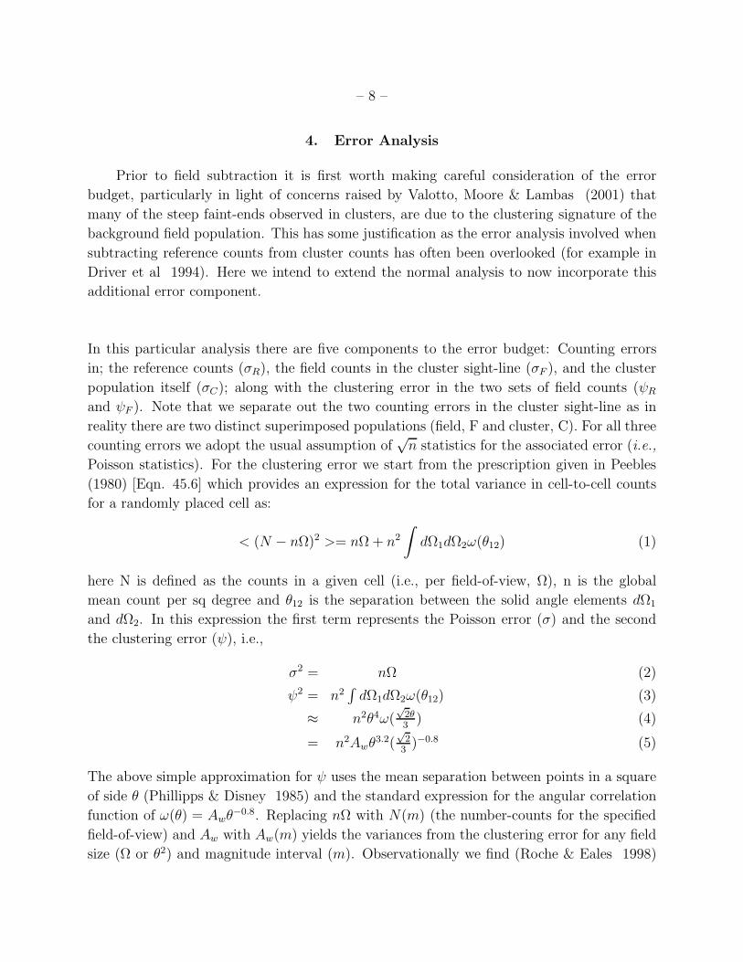
4. Error Analysis

Prior to field subtraction it is first worth making careful consideration of the error

budget, particularly in light of concerns raised by Valotto, Moore & Lambas (2001) that

many of the steep faint-ends observed in clusters, are due to the clustering signature of the

background field population. This has some justification as the error analysis involved when

subtracting reference counts from cluster counts has often been overlooked (for example in

Driver et al 1994). Here we intend to extend the normal analysis to now incorporate this

additional error component.

In this particular analysis there are five components to the error budget: Counting errors

in; the reference counts (σR), the field counts in the cluster sight-line (σF ), and the cluster

population itself (σC); along with the clustering error in the two sets of field counts (ψR

and ψF ). Note that we separate out the two counting errors in the cluster sight-line as in

reality there are two distinct superimposed populations (field, F and cluster, C). For all three

counting errors we adopt the usual assumption of√n statistics for the associated error (i.e.,

Poisson statistics). For the clustering error we start from the prescription given in Peebles

(1980) [Eqn. 45.6] which provides an expression for the total variance in cell-to-cell counts

for a randomly placed cell as:

< (N − nΩ)2 >= nΩ + n2

∫

dΩ1dΩ2ω(θ12) (1)

here N is defined as the counts in a given cell (i.e., per field-of-view, Ω), n is the global

mean count per sq degree and θ12 is the separation between the solid angle elements dΩ1

and dΩ2. In this expression the first term represents the Poisson error (σ) and the second

the clustering error (ψ), i.e.,

σ2 = nΩ (2)

ψ2 = n2∫

dΩ1dΩ2ω(θ12) (3)

≈ n2θ4ω(√

2θ3

) (4)

= n2Awθ3.2(

√2

3)−0.8 (5)

The above simple approximation for ψ uses the mean separation between points in a square

of side θ (Phillipps & Disney 1985) and the standard expression for the angular correlation

function of ω(θ) = Awθ−0.8. Replacing nΩ with N(m) (the number-counts for the specified

field-of-view) and Aw with Aw(m) yields the variances from the clustering error for any field

size (Ω or θ2) and magnitude interval (m). Observationally we find (Roche & Eales 1998)

– 9 –

that:

Aw(m) = 10−0.235mr+2.6 (6)

Hence by combining Eqns 5 & 6 and adopting (F606W − R) = 0.2—0.6 we get a final

approximation for ψ of:

ψ2 ≈ 1.83N(mF606W )210(−0.235mF606W +2.7)Ω−0.4 (7)

Assuming ω remains a power law out to the size of the field. Here N(mF606W ) are the galaxy

counts per 0.5 mag for the specified field of view, Ω, which is given in sq degrees.

The five errors identified above can now be written down explicitly as follows:

σR =√

NRΩC

3ΩR

(8)

ψR =√

3(1.83(NR/3)210(−0.235m+2.7)Ω−0.4R )ΩC

ΩR(9)

σC =√NC (10)

σF =√NF (11)

ψF =√

(1.83(NF )210(−0.235m+2.7)Ω−0.4C ) (12)

Where NR, NF and NC are the number-counts for the combined reference fields, the field

population in the A868 sight-line and the number-counts of the cluster population respec-

tively, and ΩR and ΩC are the field-of-views of the 3 individual reference fields (0.0011 sq

deg) and the cluster field-of-view (0.007545 sq deg) respectively. Where appropriate these

errors, or their adaptations, are combined in quadrature and used throughout all further

analysis steps.

5. The Morphological Luminosity Distributions of A868

The overall and morphological galaxy number-counts for the full A868 mosaic and the

combined reference fields scaled to the same area are shown on Fig. 6. Note that the A868

total counts lie above the reference field counts until mF606W ≈ 24.25 (and for each class until

mE/S0F606W ≈ 25.25, mSabc

F606W ≈ 24.75, mSd/IrrF606W ≈ 24.0), at which point the A868 counts drop

sharply indicating the approximate completeness limit(s) of the A868 data (see also Fig. 4).

We hereby adopt mF606W ≈ 24 mag as the completeness limit (equivalent to MF606W = −16

mag) and 0.75 mag brighter than the apparent completeness limit. The reference counts,

obtained from the two Hubble Deep Fields and 53W002, extend substantially deeper than

the A868 counts but provide no available data at bright magnitudes (mF606W < 21 mag).

– 10 –

To circumvent this we add in the MGC bright counts after transposing from B to F606W as

discussed in section 3. To provide continuous coverage over the full magnitude range we now

elect to represent the field counts by a second order polynomial fit5 to the combined reference

field data. As well as providing continuous coverage this has the additional advantage of

smoothing the reference data to remove unwanted structure from the 3 contributing fields.

The field data used and the resulting fits are shown in Tables 2 & 3 respectively. Note

that the data were only fitted over the magnitude range 15.75 < mF606W < 24.25 although

additional data are shown in Table 2 for completeness. The smoothing of the counts does

not reduce the associate errors but redistributes it over the specified magnitude range.

Subtracting the smoothed reference field counts from the A868 counts for each popu-

lation yields a direct statistical representation of the morphological luminosity distribution

for the cluster (adopting a universal Sab K-correction of 0.20 mags), as shown on Fig. 7

and tabulated as Table 4. Also shown on Fig. 7 (upper left, dotted line) is the 2dFGRS

composite cluster luminosity function (LF) as derived by De Propris et al (2003), shifted to

the F606W bandpass. This gives a formally acceptable fit to the cluster. The open squares

show the previous and deeper ground-based R-band data which agrees well within the er-

rors. Given that the background subtraction is derived from an entirely different region of

sky to the earlier work (see Driver et al 1998a) this provides a further indication that the

steep faint-end slope seen in A868 is a robust result. Of course one might argue that the

A868 sight-line could be contaminated by a more distant cluster, although this would boost

the faint elliptical counts/LF which is not seen. Fig. 7 shows the LFs of ellipticals (E/S0s,

upper right), spirals (Sabcs, lower left) and irregulars (Sd/Irrs, lower right). Morphological

K-corrections of K(E/S0) = 0.25, K(Sabc) = 0.20, K(Sd/Irr) = 0.11 were calculated for

the F606W filter combined with the 15Gyr evolved E, Sa and Sc model spectra of Poggianti

(1997). The formal 1, 2,& 3σ error ellipses for the Schechter function fits, based on the

χ2-minimisation of the standard Schechter LF, are shown as Fig. 7. The results and formal

1σ errors are also tabulated in Table 5. For Fig. 7 (upper left, all types) the solid line shows

the sum of the three individually derived morphological LFs showing interesting structure

consistent with recent reports of an upturn at fainter magnitudes (e.g. A0963, Driver et

al 1994) and/or a dip at intermediate mags (e.g. Coma, Trentham 1998). If each mor-

phological class has a universal LF, as has been suggested (Binggeli, Sandage & Tammann

1988), this dip then naturally arises as the morphological mix changes (as required by the

morphology-density relation, Dressler et al 1997). The errorbars shown in Fig. 7 and the re-

sulting error contours shown on Fig. 8 include the five error components discussed in section

4. It is worthwhile assessing which of these error components dominate the error budget.

5The fit is a least squares fit to the data with the errors given by Eqns. 8 and 9.

– 11 –

Fig. 9 shows the total and individual error components involved in this analysis. From this

figure we can see that the dominant error at bright magnitudes comes from the number of

cluster members, whereas at faint magnitudes the dominant error typical comes from the

clustering of the background population in the cluster sight-line. One interesting point to

note is that a full blown spectroscopic study would fail to reach the faint magnitudes probed

here, and of course be unable to improve the statistics at bright magnitudes. In fact a spec-

troscopic study is more likely to lead to additional uncertainty due to completeness issues.

Further improvement can only come from the combination of extensive deep imaging data for

a large sample of combined cluster data. Nevertheless it is clear from Fig. 7 that the steep

faint-end seen in A868 is almost entirely dominated by late-types with some contribution

from mid-types in general agreement with the findings of Boyce et al (2001).

5.1. Comparisons with the Field

Unfortunately while field morphological LFs exist, no comparison is sensible unless an

identical morphological classification methodology has been applied. However as a general

result, morphological field studies typically find α > −1 for early-types, α ≈ −1 for mid-

types and α < −1 for late-types (see for example SSRS2s morphological LFs, Marzke et al

1998; 2dFGRSs spectral LFs, De Propris et al 2003, Madgwick et al 2002; and SDSS-EDRs

morphological LFs, Nakamura et al 2003). We compare the recent results, from the SDSS-

EDR, who classify 1500 galaxies onto a similar but not identical morphological system in

r′. To adapt Nakamura et al’s numbers to provide consistent morphological LFS we added

2/3s of their Sbc-Sd class to their S0a-Sb class and 1/3 of their Sbc-Sd class to their Im

class and rederived the Schechter function parameters. We also derive (F606W − r′) =

r′ + 1.35(B − V ) − 0.95 (from Fukugita et al 1996; Liske et al 2003; and our estimate of

(BMGC − F606W ) from section 2.1) and adopt (B − V )E/S0 = 0.9, (B − V )Sabc = 0.7 and

(B − V )Sd/Irr = 0.5 (see Driver et al 1994). This gives the following morphological field

LFs:

M∗E/S0 = −21.42, αE/S0 = −0.8,

M∗Sabc = −21.35, αSabc = −1.1,

M∗Sd/Irr = −21.65, αSd/Irr = −1.9

The location of the morphological field LFs are shown on Fig. 8 as solid symbols with

errorbars. We see that the E/S0, Sabc and Sd/Irr field and cluster LFs are all consistent at

the 1σ-level (and in qualitative agreement the field and cluster LFs of Binggeli, Sandage &

Tammann (1988)). Clearly though the errors dominate and many clusters must be studied

– 12 –

in a combined analysis before the universality of morphological luminosity functions can

be confirmed or refuted. Given the extensive SDSS-EDR database and the incoming ACS

cluster data this is likely to be established in the near future and the current results should

be taken as indicative that the morphological LFs are not widely variant between cluster

and field environments.

6. The Morphological Radial Distributions of A868

We now subdivide the mosaic into five radial intervals of 0.75′ (130 kpc) around the

dominant cD, and calculate the contribution of each morphological class to the luminosity-

and number- density within the range 15.9 < mF606W < 23.9 mag (equivalent to −24 <

MF606W < −16 mag). To achieve this we build a map of the mosaic to calculate the relevant

active fields-of-view, within each annulus, and use the expressions given in Table 3 to subtract

off the appropriate field component. Fig. 10 (upper) shows the radial dependency of the

luminosity-density, j, for each type in arbitrary units and Fig. 10 (lower) the number-density.

Whereas the former is skewed towards brighter systems (which dominate the luminosity-

density) the latter is skewed towards fainter systems (at least for mid- and late- type spirals

which have rising LFs). From Fig. 10 we find a number of indicative results. First though, we

note the rise in luminosity-density and number-density in the final radial bin. This is likely

because of the presence of the second D galaxy which lies 0.7 Mpc from the central cD and

may represent an infalling sub-group. Ignoring the bias introduced by this last bin we find

that the luminosity-density of each class falls in a near linear fashion in log(j) versus radius

with gradients of: −0.68±0.06, −0.32±0.06, −0.30±0.18, for E/S0+cD/D, Sabc and Sd/Irr

respectively. Ignoring the cD/D galaxies results in a gradient of −0.41± 0.08, for the E/S0s

alone (i.e., consistent with the mid-type population). This is of course an independent

confirmation of the well known morphology-density relation Dressler et al (1997). Note

that the exclusion of the cD/Ds has little impact upon the derived Schechter function for

early-types, (c.f. dashed line on Fig. 8, middle, E/S0s, see also Table 5). Similarly the

number-densities also fall near linearly in log(N) versus radius with a significant variation

in gradient depending on type (−0.68± 0.21, −0.28± 0.08, +0.02± 0.07, for E/S0+cD/Ds,

Sabcs and Sd/Irrs respectively)6.

From Fig. 10 two clear conclusions can be drawn. Firstly the classical result that early-

type galaxies are more centrally concentrated in number than mid-type spirals which in turn

6Note that a projected profile with ρ ∝ r−k is roughly equivalent to a real profile of ρ ∝ r

−1−k, hence

the positive projected profile for Sd/Irrs still implies a decreasing 3D radial profile.

– 13 –

are more centrally concentrated than late-type irregulars. Secondly the flat number-density

profile of late-types implies that the core must be devoid of late-types which therefore exist

exclusively in the cluster halo, independently confirming the result of Boyce et al (2001).

This halo extends beyond the field-of-view studied here but from the luminosity-density

profile it is unlikely to contribute significantly to the total luminosity-density at any radii.

Within the field-of-view studied we note that the total luminosity-density, within all annuli,

is divided into (72 ± 13) per cent E/S0+cD/Ds, (26 ± 3) per cent Sabcs, and (2 ± 1) per

cent Sd/Irrs. This can be compared to those derived from the SDSS-EDR field LFs shown

above (where j = φ∗L∗Γ(α+2)) of 29 per cent, 59 per cent, and 12 per cent for early-, mid-,

and late- types respectively. Neglecting the cD/Ds changes the cluster percentages to 63 per

cent, 34 per cent and 3 per cent respectively (with similar errors).

As a comparison we note that values of 33 per cent, 53 per cent, and 14 per cent for the

field were derived by Driver (1999) for a volume limited sample at z ≈ 0.45 drawn from the

Hubble Deep Field and classified using the same ANN classifiers as used here. The consensus

between these two independent field studies is reassuring and provides some indication of the

associated errors. If one assumes that both the field and cluster environments originate from

an identical shape primordial mass spectrum but with differing amplitudes, this discrepancy

must be due to an additional/accelerated evolutionary mechanism(s) over those at work

in the field. From this data alone one cannot argue factually for the exact nature of this

mechanism other than it has the net effect of converting later types towards earlier types, and

is most efficient in the cluster core. In fact if one crudely adopts conservation of luminosity

(strictly more valid at longer wavelengths) then up to 50 per cent of the ellipticals must

have been formed from mid- or late- type spirals. This requires some contrivance given the

apparent universality of the morphological LFs between the field and A868 environment

although far more data for both field and clusters are required before any real significance

can be attached to the difference seen, as well as a more fully consistent classification scheme.

In general the results here are consistent with the conventional picture whereby the

core environment is hostile to disks and converts mid-types to early-types — which remain

captured in the core — and destroys late-types entirely as they transit through the core.

7. Conclusions

We report the first reconstruction of morphological luminosity functions for a cluster

environment since the founding work of BST. Through the method of background subtraction

we recover the overall LF seen for A868 in a previous ground-based study, but which used

an entirely different region of sky for the background subtraction, this adds credence to the

– 14 –

methodology of background subtraction for this very rich cluster at least. In our analysis we

lay down a methodology for accounting for background clustering bias missing in previous

analysis of this type and addressing concerns raised by Valotto, Moore & Lambas (2001).

The overall cluster LF is comparable to the general field LF (2dFGRS) and we find that

the early-, mid- and late- type LFs are all consistent with the field LFs. However the errors

are such that one can not yet argue convincingly for, or against, ubiquitous morphological

LFs as proposed by BST.

In exploring the luminosity- and number- density radial profiles we find flat profiles for

late-types and argue that this implies an absence of late-type galaxies in the core region.

Furthermore we find a significantly skewed luminosity-density breakdown towards early-

types, as compared to the field. We speculate that this implies that cluster cores are in

essence disk-destroying engines resulting in the build up of a hot inter-cluster member and

the formation of a tightly bound population of intermediate-luminosity core ellipticals most

likely formed from mid-type bulges.

Finally from our error analysis we note that more definitive results can only be obtained

from the combination of cluster data, as the dominant error at bright magnitudes is simply

the number of cluster members. Such data is is now becoming freely available via the Sloan

Digital Sky Survey and the Hubble Space Telescope Archives. In this paper we have laid down

a rigorous methodology for the analysis of such data and look forward to an illuminating

era.

We would like to thank Ray Lucas for help with the planning of the observations and

Roberto De Propris and an anonymous referee for helpful comments on the manuscript.

Support for program #8203 was provided by NASA through a grant from the Space Tele-

scope Science Institute, which is operated by the Association of Universities for Research in

Astronomy, Inc., under NASA contract NAS 5-26555.

REFERENCES

Baldry, I., et al, 2002, ApJ, 569, 582

Barkhouse, W.A., & Yee, H.C., in Tracing Cosmic Evolution with Galaxy Clusters. ASP Con-

ference Proceedings 268, ed. S. Borgani, M. Mezzetti, R. Valdarnini (San Fransisco:

Astronomical Society of the Pacific), p 289,

Bertin, E., & Arnouts, S., 1996, A&AS, 117, 393

– 15 –

Bingelli, B., Sandage, A., & Tammann G.A., 1988, ARA&A, 26, 509

Boyce, P., Phillipps, S., Jones, J.B., Driver, S.P., Smith, R.M., & Couch, W.J., 2001, MN-

RAS, 328, 277

Bower, R.G., & Balogh, M.L., 2003, in Clusters of Galaxies: Probes of Cosmic Structure

and Evolution. eds. J. S. Mulchaey, A. Dressler, A. Oemler, (Publ: Cambridge Univ.

Press), in press

Christlein, D., & Zabludoff, A., 2003, ApJ, in press

Cohen, S., Windhorst, R.A., Odewahn, S.C., Chiarenza, C.A., & Driver, S.P., 2003, AJ, in

press

Cross, N.J.G., Driver, S.P., Liske, J., & Lemon, D.J., 2003, MNRAS, submitted

De Propris, R., et al, 2003, MNRAS, in press

de Vaucouleurs, G., de Vaucouleurs, A., Corwin, H.G., Buta, R.J, Paturel, G., & Fouque,

P., 1995, The Third Reference Catalogue of Galaxies, (Publ: Springer-Verlag)

Dressler, A., 1980, ApJ, 236, 351

Dressler, A., Oemler, A., Couch, W.J., Smail, I., Ellis, R.S., Barger, A., Butcher, H., Pog-

gianti, B., & Sharples, R.M., 1997, ApJ, 490, 577

Driver, S.P., Phillipps, S., Davies, J.I., Morgan, & Disney, M.J., 1994, MNRAS, 268, 393

Driver, S.P., & De Propris, R., 2003, Astro. Lett & Comm., in press

Driver, S.P., Couch, W.J., & Phillipps, S., 1998a, MNRAS, 301, 369

Driver, S.P., Couch, W.J., Phillipps, S., & Smith, R.M., 1998b, MNRAS, 301, 357

Driver, S.P., Windhorst, R.A., Ostrander, E.J., Keel, W.M., Griffiths, R.E., & Ratnatunga,

K.U., 1995, ApJ, 449, 23

Driver, S.P., 1999, ApJL, 526, 69

Fukugita, M., Ichikawa, T., Gunn, J. E., Doi, M., Shimasaku, K., & Schneider, D.P., 1996,

AJ, 111, 1748

Fruchter, A.S., & Hook, R., 2002, PASP, 114, 144

Gomez, P., et al., 2003, ApJ, in press

– 16 –

Holtzmann, J.A., Burrows, C.J., Casertano, S., Hester, J.J., Trauger, J.T., Watson, A.M.,

& Worthey, G., 1995, PASP, 107, 1065

Lewis, I., et al 2002, MNRAS, 334, 673

Liske, J., Lemon, D.J., Driver, S.P., Cross, N.J.G., & Couch, W.J., 2003, MNRAS, in press

Lopez-Cruz, 1997, PhD University of Toronto

Madgwick, D.S., et al, 2002, MNRAS, 333, 133

Marzke, R.O., da Costa, L.N., Pellegrini, P.S., Willmer, C.N.A., & Geller, M.J., 1998, ApJ,

503, 617

Moore, B., Lake, G., & Katz, N., ApJ, 499, 5

Nakamura, O., Fukugita, M., Yasuda, N., Loveday, J., Brinkmann, J., Schneider, D.P.,

Shimasaku, K., & SubbaRao, M., 2003, ApJ, in press

Norberg, P., et al 2002, MNRAS, 336, 907

Odewahn, S.C., Windhorst, R.A., Driver, S.P., & Keel, W.C., 1996, ApJ, 472, 13

Odewahn, S.C., Cohen, S., Windhorst, R.A., & Ninan Sajeeth, P., 2002, ApJ, 568, 539

Peebles, J.P.E., 1980, in The Large Scale Structure of the Universe, (Publ: Princeton)

Phillipps, S., Disney, M.J., 1985, A& A, 148, 234

Phillipps, S., Driver, S.P., Couch, W.J., & Smith, R.M., 1998, ApJ, 498, 119

Poggianti, B., 1997, A&AS, 122, 399

Pracy, M., de Propris, R., Couch, W.J., Bekki, K., Driver, S.P., & Nulsen P.E.J., 2003,

MNRAS, submitted

Roche, N., & Eales, S., 1998, MNRAS, 307, 703

Sabatini, S., Davies, J., Scaramella, R., Smith, R.M., Baes, M., Linder, S., Roberts, S., &

Testa, V., MNRAS, in press

Sandage, A., Bingelli, B., & Tammann G.A., 1985, AJ, 90, 1759 (BST)

Schlegel, D., Finkbeiner, D.P., & Marc, D., 1998, ApJ, 500, 525

Smith, R.M., Driver, S.P., & Phillipps, S., 1997, MNRAS, 287, 415

– 17 –

Strubble, M.F., & Rood, H.J., 1999, ApJS, 125, 35

Sung, H., & Bessell, M.S., 2000, PASA, 17, 244

Thompson, L.A., Gregory, S.A, 1993, AJ, 106, 2197

Trentham, N., 1998, MNRAS, 295, 360

Trentham, N., & Tully, B., 2002, MNRAS, 335, 712

Trentham, N., & Hodgkin, S., 2001, MNRAS, 333, 423

Valotto, C.A., Moore, B., & Lambas, D.G., 2001, ApJ, 546, 157

Windhorst, R.A., Keel, W.C., & Pascarelle, S., 1998, ApJ, 494, 27

This preprint was prepared with the AAS LATEX macros v5.0.

– 18 –

Fig. 1.— The full six pointing mosaic of the A868 cluster and environs. North is up with

East to the left. The box is 6.62 arcminutes (or 1.08 Mpc at z = 0.158) on each side. The

cluster core is clearly visible and shown in more detail in Fig.2.

Fig. 2.— A single WFPC2 chip showing the core of the rich cluster A868. The image is

approximately 1.5 arcminutes on each side (0.25 Mpc). Clearly visible is the central cD and

one of the D galaxies with numerous examples of gravitational lenses.

Fig. 3.— Total versus isophotal magnitudes for the full A868 mosaic. The cD/Ds, early-,

mid- and late-types are denoted as filled circles, open circles, filled squares and open triangles

respectively. The dotted line shows the adopted cap to the isophotal corrections. (Note that

the one spiral furtherest from the unity line lies close to a bright elliptical resulting in the

extreme isophotal correction.)

Fig. 4.— The apparent bivariate brightness distribution for galaxies in the A868 sight-line.

The effective surface brightness is derived from the measured major-axis half-light radius

(µeff = m + 2.5 log10(2πr2hlr)). Large filled circles denote cD/Ds, open circles early-types,

filled squares mid-types, triangles late-types and crosses stars. The dashed lines denote the

limiting surface brightness and star-galaxy separation limit.

Fig. 5.— A random sample of stars, early-, mid- and late- types (across) versus apparent

magnitude (down).

Fig. 6.— Cluster sight-line and reference field counts (scaled to the A868 field-of-view size

of 0.007545 sq degrees). Counts are shown for all galaxies, early-, mid- and late-types. The

solid lines shows a 2nd order polynomial fit to the field count data. Errors are purely Poisson

at this point.

Fig. 7.— The recovered luminosity distributions for the cluster population after subtracting

the reference field counts from the A868 sight-line counts. The errorbars now include the

full error analysis (i.e., five error components including 3 Poisson and 2 clustering errors).

The solid lines show the χ2-minimised Schechter function fits to the data. In the case of all

galaxies we also show the 2dFGRS composite cluster luminosity function ((De Propris et al

2003)) transposed to the F606W filter and renormalized to match the data. The squares

show the previous deeper R-band cluster results from Driver et al (1998a).

Fig. 8.— The 1, 2 and 3 σ error contours for the Schechter function fits shown in Fig.9.

The crosses shows the actual best fit points. The solid points with errorbars show the recent

field estimates based on SDSS-EDR data by Nakamura et al 2003. The open data point

shows the recent composite cluster LF estimated from the 2dFGRS (De Propris et al 2003),

– 19 –

errors are comparable to the symbol size. For the ellipticals the solid contours show the fit

to E/S0s+cD/Ds and the dotted contours the fits to E/S0s only.

Fig. 9.— The five error components to the cluster luminosity distributions for all galaxies,

ellipticals, early-type and late-type galaxies. In most cases the Poisson error in the cluster

population dominates at brighter magnitudes and the clustering error in the field population

dominates at faint magnitudes.

Fig. 10.— (upper) The luminosity-density profiles derived from the absolute magnitude

range −24 < MF606w < −16 for all (crosses, solid), cD/D+E/S0 (pentagons, dotted line),

E/S0 (circles, dotted line), Sabc (squares, short dashed), Sd/Irr (triangles, long dashed

line) in arbitrary units in five annuli centered around the central cD galaxies. (lower) The

equivalent number-density profiles labeled as above.

.

– 20 –

Table 1. Summary of morphological classification overrides

Ellipticals Early-types Late-types Stars

Ellipticals - 4 0 2

Early-types 2 - 20 0

Late-types 1 32 - 0

Stars 2 3 1 -

Junk 2 11 2 6

– 21 –

Table 2. Number Count data for all, early-, mid- and late- type reference field galaxies

per 0.007545 sq degrees. The errors include both Poisson and clustering components

mag N(All) N(E/S0) ∆N(Sabc) ∆N(Sd/Irr)

15.190 0.016 + /− 0.003 0.003 + /− 0.001 0.010 + /− 0.002 0.003 + /− 0.001

15.690 0.030 + /− 0.005 0.011 + /− 0.002 0.012 + /− 0.003 0.006 + /− 0.002

16.190 0.057 + /− 0.009 0.020 + /− 0.004 0.028 + /− 0.005 0.009 + /− 0.002

16.690 0.115 + /− 0.015 0.041 + /− 0.006 0.060 + /− 0.008 0.013 + /− 0.002

17.190 0.202 + /− 0.023 0.066 + /− 0.008 0.104 + /− 0.012 0.032 + /− 0.004

21.450 23.003 + /− 8.751 4.601 + /− 3.395 9.201 + /− 5.061 4.601 + /− 3.395

21.750 32.204 + /− 10.655 6.901 + /− 4.205 13.802 + /− 6.346 9.201 + /− 4.938

22.050 29.904 + /− 9.886 2.300 + /− 2.337 16.102 + /− 6.849 11.502 + /− 5.544

22.350 46.006 + /− 12.811 9.201 + /− 4.847 16.102 + /− 6.740 18.402 + /− 7.187

22.650 64.409 + /− 15.664 13.802 + /− 6.018 18.402 + /− 7.187 16.102 + /− 6.566

22.950 59.808 + /− 14.452 11.502 + /− 5.394 34.505 + /− 10.357 13.802 + /− 5.962

23.250 62.108 + /− 14.432 11.502 + /− 5.357 34.505 + /− 10.154 20.703 + /− 7.409

23.550 85.111 + /− 17.329 25.303 + /− 8.212 29.904 + /− 9.162 27.604 + /− 8.631

23.850 142.619 + /− 24.035 16.102 + /− 6.342 32.204 + /− 9.436 71.309 + /− 15.048

24.150 190.925 + /− 28.632 18.402 + /− 6.773 55.207 + /− 12.822 98.913 + /− 18.157

24.450 246.133 + /− 33.231 13.802 + /− 5.783 73.610 + /− 15.030 156.421 + /− 24.024

24.750 280.637 + /− 35.223 9.201 + /− 4.670 75.910 + /− 15.027 158.721 + /− 23.569

25.050 437.058 + /− 47.259 16.102 + /− 6.221 112.715 + /− 18.849 220.829 + /− 28.661

25.350 558.974 + /− 54.724 16.102 + /− 6.201 200.127 + /− 26.792 331.244 + /− 36.906

25.650 565.875 + /− 52.836 9.201 + /− 4.643 211.628 + /− 27.051 365.748 + /− 38.259

– 22 –

Table 3. 2rd order polynomial fits to the field number-count data over the range

15 < m < 24.25

Fit χ2/ν

log10N(All)dm = −14.752 + 1.103mF606W − 0.0166m2F606W 7.8/12

log10N(E/S0)dm = −18.595 + 1.484mF606W − 0.0273m2F606W 10.0/11

log10N(Sabc)dm = −16.770 + 1.290mF606W − 0.0215m2F606W 10.0/12

log10N(Sd/Irr)dm = −11.491 + 0.639mF606W − 0.0035m2F606W 14.2/11

Table 4. The estimated cluster population for all, early-, mid-, and late- type A868

cluster galaxies per 0.007545 sq degrees. The errors include both Poisson and clustering

components

mag N(All) N(E/S0) N(Sabc) N(Sd/Irr)

16.00 −0.05 + /− 1.07 −0.01 + /− 1.02 −0.02 + /− 1.04 −0.01 + /− 1.01

16.50 0.91 + /− 1.10 0.97 + /− 1.03 −0.05 + /− 1.07 −0.01 + /− 1.02

17.00 1.84 + /− 1.55 1.94 + /− 1.46 −0.09 + /− 1.14 −0.02 + /− 1.04

17.50 2.70 + /− 1.94 2.89 + /− 1.80 −0.16 + /− 1.25 −0.04 + /− 1.07

18.00 6.46 + /− 2.90 2.81 + /− 1.86 3.70 + /− 2.18 −0.08 + /− 1.13

18.50 10.03 + /− 3.69 7.67 + /− 2.97 2.47 + /− 2.09 −0.14 + /− 1.22

19.00 15.32 + /− 4.67 9.43 + /− 3.38 6.07 + /− 3.07 −0.26 + /− 1.37

19.50 5.13 + /− 4.08 3.06 + /− 2.52 1.42 + /− 2.69 0.54 + /− 1.46

20.00 18.19 + /− 6.20 8.51 + /− 3.72 10.38 + /− 4.51 −0.83 + /− 1.96

20.50 20.10 + /− 7.43 9.69 + /− 4.25 10.75 + /− 5.23 −0.47 + /− 2.48

21.00 7.25 + /− 8.20 −1.46 + /− 3.71 8.29 + /− 5.95 0.40 + /− 3.12

21.50 17.84 + /− 10.89 1.97 + /− 4.55 9.67 + /− 7.26 6.41 + /− 4.83

22.00 30.70 + /− 14.03 −3.09 + /− 5.25 20.47 + /− 9.34 13.94 + /− 6.69

22.50 21.34 + /− 17.02 −5.67 + /− 6.12 10.23 + /− 10.52 17.90 + /− 8.61

23.00 39.80 + /− 21.54 −8.79 + /− 7.02 12.44 + /− 12.63 37.43 + /− 11.88

23.50 55.65 + /− 26.65 −4.38 + /− 7.92 10.57 + /− 14.81 49.35 + /− 15.55

24.00 66.95 + /− 32.43 −7.34 + /− 8.78 42.17 + /− 18.15 26.27 + /− 19.69

– 23 –

Table 5. Derived Schechter function parameters for the overall and morphological

luminosity distributions of the Rich cluster Abell 868.

Morphological T-type φ∗h30.65 M∗

F606W − 5log10h0.65 α χ2/ν

Class Range (0.007545 sq deg−1) (mag)

All −6 < T < 9 16.4 −22.4+0.6−0.6 −1.27+0.13

−0.15 8.8/12

E/S0+cD/D −6 < T ≤ 0 29.2 −21.6+0.6−0.5 −0.51+0.2

−0.3 7.9/7

E/S0 −6 < T ≤ 0 41.2 −20.9+0.4−0.4 −0.13+0.4

−0.4 6.9/5

Sabc 0 < T ≤ 6 14.0 −21.3+1.0−0.9 −1.19+0.2

−0.2 6.0/10

Sd/Irr 6 < T ≤ 9 89.7 −17.4+0.7−0.7 −1.40+0.6

−0.5 0.7/4

– 24 –

– 25 –

– 26 –

16 17 18 19 20 21 22 23 24 25 26 2716

17

18

19

20

21

22

23

24

25

26

27

F606W isophotal magnitudes

– 27 –

16 17 18 19 20 21 22 23 24 25 2626

25

24

23

22

21

20

19

18

17

16

15

14

F606W app. mag

– 28 –

– 29 –

16 18 20 22 24 26

0.1

1

10

100

1000

F606W app. mag.

All galaxies

Cluster Field

16 18 20 22 24 26

0.1

1

10

100

1000

F606W app. mag.

E/S0

16 18 20 22 24 26

0.1

1

10

100

1000

F606W app. mag.

Sabc

16 18 20 22 24 26

0.1

1

10

100

1000

F606W app. mag.

Sd/Irr

– 30 –

– 31 –

-24 -22 -20 -18 -162

1

0

-1

-2 All

2dFGRSSDSS-EDR

-24 -22 -20 -18 -162

1

0

-1

-2 E/S0+cD/DsE/S0

-24 -22 -20 -18 -162

1

0

-1

-2 Sabc

-24 -22 -20 -18 -162

1

0

-1

-2

Sd/Irr

– 32 –

– 33 –

All

E/S0+cD/D

E/S0

Sabc

Sd/Irr