Loss of Linearity and Symmetrisation inRegulatory Networks

Jacques Demongeot1, Eric Goles2,3, and Sylvain Sene4,5

1 UJF-Grenoble, TIMC-IMAG, Faculte de Medecine, 38706 La Tronche cedex, France2 Universidad Adolfo Ibanez, Penalolen, Santiago, Chile

3 ISCV, Institute for Complex Systems, Av. Artillerıa 600B, Cerro Artillerıa,Valparaıso, Chile

4 Universite de Lyon, INSA-Lyon, LIRIS, F-69621, France5 IXXI, Institut rhone-alpin des systemes complexes, 5, rue du Vercors, 69007 Lyon,

France

Abstract. This article aims at giving some new theoretical propertiesof threshold Boolean automata networks which are good mathematicalobjects to model biological regulatory networks. The objective is the em-phasis of a necessary condition for which these networks, when they aregoverned by a non-linear evolution law, are sensitive to the influence ofboundary conditions. Then, this paper opens an argued discussion aboutthe notion of “symmetrisability” of regulatory networks which is relevantto understand some specific dynamical behaviours of real biological net-works, and shows that this notion allows to explain an important featureof the Arabidopsis thaliana floral morphogenesis model.

Keywords: Stochastic and deterministic regulatory networks; Robust-ness; Boundary conditions; Symmetrisation.

1 Introduction

More and more studies have been opened since a decade about the robust-ness of biological regulatory networks [1,2]. This is explained by the fact therobustness against several kinds of perturbations, such as changes of updatingmodes [3,4] or changes of topology [5], may bring a better understanding ofparticular phenomena emerging in biology. The purpose of this paper is to showthat, sometimes, a theoretical framework allows to obtain some results which areof great interest not only in this theoretical framework but also in applied frame-works. Moreover, we think that studies on real biological regulatory networks,whatever the used mathematical objects are, need a deep theoretical attention.Indeed, if it is possible to dive a real biological network in a specific frameworkwith relevant theoretical tools, we can reasonably expect to obtain some resultson inherent properties of this biological network which could not be obtainedwith an empirical method.

After a brief section presenting the main definitions which will be used in thispaper, Section 3 focuses on artificial stochastic regulatory networks representedby square lattices on Z2. It extends some results already obtained [6,7] on the

impact of variations of boundary conditions on stochastic regulatory networkswhose evolution is governed by a non-linear law and presents a necessary condi-tion for which phase transitions can emerge. These results are interesting fromboth the theoretical and biological points of view. Indeed, biological regulatorynetworks present in general natural boundaries such as hormones or microRNAsin general inhibiting the expression of some genes inside the network (some casesof activation being also described as in [8]). Section 4 gives an argued discussionabout the dynamical behaviour of the well known Mendoza genetic regulatorynetwork for the floral morphogenesis of the plant Arabidopsis thaliana [9] andshows that it is a direct consequence of its underlying threshold Boolean au-tomata network, which can be seen as a symmetric network.

2 Preliminaries

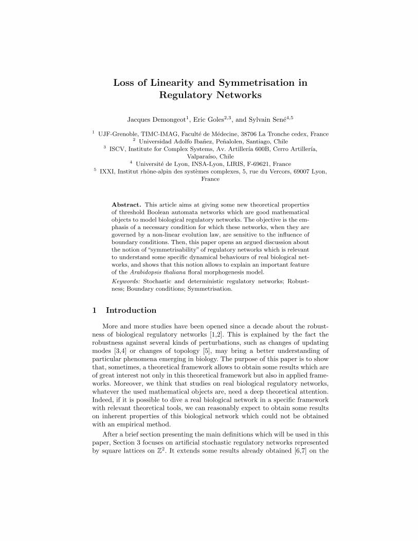
Artificial regulatory networks are widely used in systems biology and presentremarkable regularities in their architecture due to the evolution [10,11,12],namely similar values for architectural (connectivity) or dynamic features, oroccurrence of same interaction motifs [3], i.e., oriented sub-graphs relating theirelements (here genes). These similarities cause identical dynamical behaviours,like existence of periodic attractors, called limit cycles due for example to thesame internal motif imposing its periodicity to the global network. Biologicalregulatory networks are less regular than artificial ones (see Figure 1) but theyshare many common dynamical concepts that we will give first in whole gener-ality.

(a) (b) (c) (d)

Fig. 1. Representations of oriented interaction graphs of biological (a, b) andartificial (c, d) regulatory networks.

The interaction matrix W of a regulatory network R of n genes is the orientedand valued incident n × n matrix of its interaction graph. W is then similar tothe synaptic weights matrix, which rules the relationships between neurons in aneural network. The general coefficient wik of such a matrix W is positive (resp.negative, null) if the gene k activates (resp. inhibits, does not influence) the genei, the state xi of i being equal to 1 (resp. 0), if it is (resp. is not) expressed. Inthe sequel, we consider two different kinds of regulatory networks, called eitherdeterministic or stochastic. Precisely, in a deterministic regulatory network, thechange of state of a gene i between times t and t + 1 is supposed to obey the

deterministic transition rule [13,14]:

∀i ∈ R, xi(t+ 1) = H(∑j∈Ni

wij · xj(t)− θi)

or

x(t+ 1) = H(W · x(t)− θ)

whereH is the classical Heaviside sign-step function (H(x) = 0 if x < 0 and 1 otherwise),Ni is the set of neighbours of i such that j ∈ Ni ⇐⇒ wij 6= 0 and θi is theactivation threshold of i. In a general way, it is of great biological interest to de-termine interaction matrices having characteristic properties like: (i) a minimalnumber of non zero coefficients for a given set of attractors or (ii) a minimalnumber P (W ) of positive loops (i.e. paths on the interaction graph coming froma gene and returning to it after an even number of negative interactions) countedonly one time, which controls the number A(W ) of attractors [15,16]. The con-

nectivity coefficient K(W ) = I(W )n is the mean number of interactions going

to a gene, where I(W ) is the total number of interactions: K(W ) is in generalbetween 1.5 and 3. About the number C(W ) of strong connected components(i.e. with a path between each pair of genes in both senses) containing positiveloops, we can conjecture (in particular for feed-forward networks) that:

2P (W ) ≥ A(W ) ≥ 2C(W ) and A(W ) ≥ O(n12 )

The total number of attractors is, in the general case, of greater order of mag-nitude, due to the presence of numerous limit cycles both in Hopfield-like (resp.Kauffman-like) random regulatory networks in which the 43 different sets of in-teraction signs 1, −1 or 0 (resp. the 16 possible sets of Boolean functions) arerandomly chosen for the nearest neighbours of any node in the transition rule[42,43].

In the case of stochastic regulatory networks, the introduction of randomnessis done by a specific parameter called the temperature, denoted by T . By con-sidering the same transition operator as above Rx = H(Wx − θ), we computethe probability for the gene i to be in state 1 at time t+ 1 knowing the state ofits neighbours at time t:

∀i ∈ R, P (xi(t+ 1) = 1) =eRx/T

1 + eRx/T

If T is sufficiently large, this probability is 1/2 (uniform case) and if T is suf-ficiently small, the stochastic network has the same behaviour as the networkwith the deterministic transition rule given above. When T is small, we retrievethe deterministic rule. Nevertheless, the real link between the stochastic andthe deterministic rules is not actually well known. In this context, we give thefollowing proposition:

Proposition 1. If T is small and ∀i, j ∈ Zd, wii = u0 > θ,wij = u1 > 0 ifδ(i, j) = 1, and wij = 0 if δ(i, j) > 1, where δ is the L1-distance on Zd, then

the mean probability α(T ) to change from state 1 to state 0 at time t+ 1, with auniform initial distribution over the a = |Ni\{i}| nodes of Ni\{i}, is given by:

α(T ) = e(−u0+θ)/T · [(1 + e−u1/T )/2]a

Proof: Let us denote C = {xi(t) = 1; xj(t) = yj ; j ∈ Ni\{i}} and develop:

α(T ) =∑

y∈Ni\{i}

P (xi(t+ 1) = 0|C)2a

≈a∑k=0

(ak

)e(−u0+θ)/T−ku1/T )

2a

= e(−u0+θ)/T · [(1 + e−u1/T )/2]a

Let us note that the value above gives an estimation of the ”noise” introducedby the stochastic transition on the deterministic one where the state 0 is in thiscase never reached. �

Before going further, let us give some definitions about the notion of updatingmodes. An updating mode is: (i) parallel if, at each time step t, all the nodes of Rare updated synchronously, (ii) sequential if, at each time step, only one node ofR is updated, such that all the nodes are updated after n time steps, according toa specific sequence, (iii) block-sequential if, when the network R is divided intodisjoint subsets of nodes, the nodes in a same subset execute their local transitionfunction synchronously and the subsets are updated sequentially. Let us remarkhere that the parallel and the sequential updating modes are particular block-sequential modes. Furthermore, in the context of artificial networks representedby square lattices on Z2, the centre of a regulatory network is the set of minimaleccentricity nodes (the eccentricity ε(u) of the vertex u of a connected orientedinteraction graph G = (V,E) is the maximal distance from u to any other nodesv of G) and its boundary is simply the set of all geometric boundary nodes ofthe underlying lattice.

3 Loss of linearity in stochastic networks

Some relevant studies [17,6,7] have been recently done on the influence ofboundary conditions on two-dimensional square lattices showing both theoret-ically and by simulation a specific condition under which stochastic thresholdBoolean networks are strongly subjected to variations of their boundary con-ditions. These studies have been based on a specific kind of networks evolu-tion which is characterised by the linear stochastic transition function presentedabove. Indeed, the networks elements update their state from the time step t tothe time step t + 1 according to two different potentials: u0, a function of theauto-interaction weight, and u1, a function of the closest neighbours interactionweights. Here, we propose to study two-dimensional square lattices governed bya stochastic law taking also into account a collective potential, denoted by φ,

which is going to be detailed in the following. Let us remark that the introduc-tion of this coalition potential is translated by a loss of linearity of the stochastictransition function, which makes this kind of problem much more difficult.

Let us first remark that, when time t tends to infinity, the occurrence of con-figurations is given by an invariant measure µ on the space of all configurations,which depends on the updating mode of the network. In [17,7] has been givena general expression of µ, for an arbitrary given feed-forward network R of nnodes, for the general block-sequential updating mode. The notion of invariantmeasure is of particular interest because it allows to define the notion of phasetransitions [18]. Indeed, being given a network R, a phase transition emergesfrom the dynamics of R, when, for two different fixed boundary conditions ∂R1

and ∂R2, two different invariant measures µ∂R1 and µ∂R2 are computed, i.e. theinvariant measure is not unique.

Let us now denote by Λ = R\{O}, where O is one of the central points ofthe interaction graph (R,E) and define the cylinder [A,B] as follows:

[A,B] = {σ | σi = 1, i ∈ A;σi = 0, i ∈ B]

The matricial projectivity equation between the probabilities of configurationson Λ is defined, as in [17], by the matrix M below:

M =

1 1 0 . . . 0 . . . 01 0 1 . . . 0 . . . 01 0 0 . . . 0 . . . 0...

......

......

......

0 0 0 . . . 0 . . . 1Φ0 Φ1 Φ2 . . . ΦK . . . Φ2d

where Φ0 = Φ(Λ, ∅), Φ1 = Φ(Λ\{1}, {1}), Φ2 = Φ(Λ\{2}, {2}), ΦK = Φ(Λ\K,K),and Φ2d = Φ(∅, Λ). In this matrix, the first equations represent the classical pro-jectivity: ∀i ∈ Λ\K, µ([Λ\K,K]) + µ([Λ\(K ∪ {i}),K ∪ {i}]) = µ([Λ\(K ∪{i}),K]), where µ([Λ\K,K]) is the probability to observe the configuration[Λ\K,K], i.e. the state 1 on Λ\K and 0 on K. The last equation is just theBayes formula, i.e. if Φ([Λ\K,K]) denotes the probability to observe the state 1in O knowing the configuration [Λ\K,K], we have:∑

K

Φ(Λ\K,K) · µ([Λ\K,K]) = µ([i, ∅])

By developing detM with respect to the last row, we have:

detM =∑K

(−1)|Λ\K| · Φ(Λ\K,K)

where (−1)|Λ\K| · Φ(Λ\K,K) + (−1)|K| · Φ(K,Λ\K) = (−1)|K|(Φ(Λ\K,K) +Φ(K,Λ\K)), because |Λ| = 2 · d, with:

Φ(K,Λ\K) =e(u0+

∑i∈K u1,i+φ(K))/T

1 + e(u0+∑i∈K u1,i+φ(K))/T

where the potential φ is symmetrical, i.e. verifies:

φ(K) = φ(Λ)− φ(Λ\K) =∑i,j∈Ki6=j

u2,i,j +∑

i,j,k∈Ki6=j 6=k

u3,i,j,k

which is the case if the u2,i,j ’s (resp. u3,i,j,k’s) are constant and equal to u2 (resp.−u2).

Proposition 2. If the singleton potential (or external field) u0, and the pair,triple and quadruple potentials, respectively denoted by u1,i’s, u2,i,j’s and u3,i,j,k’s,verify:

u0 +∑i∈Λ

u1,i2

+∑i,j∈Ki6=j

u2,i,j2

+∑

i,j,k∈Ki6=j 6=k

u3,i,j,k2

= 0

then detM = 0.

Proof: In order to prove that detM = 0, it suffices to multiply in the definitionformula of Φ(K,Λ\K) the numerator and the denominator by:

1 =e(−2u0−

∑i∈Λ\K ui−φ(Λ))/T

e(−2u0−∑i∈Λ\K ui−φ(Λ))/T

Then we have:

Φ(K,Λ\K) =e−u0−

∑i∈Λ\K ui+φ(K)−φ(Λ)

T

e−2u0−

∑i∈Λ ui−φ(Λ)

T + e−u0−

∑i∈Λ\K ui+φ(K)−φ(Λ)

T

=e−u0−

∑i∈Λ\K ui−φ(Λ\K)

T

1 + e−u0−

∑i∈Λ\K ui−φ(Λ\K)

T

= 1− eu0+

∑i∈Λ\K ui+φ(Λ\K)

T

1 + eu0+

∑i∈Λ\K ui+φ(Λ\K)

T

= 1− Φ(Λ\K,K)

Thus, we have Φ(Λ\K,K) + Φ(K,Λ\K) = 1, and, since we have |Λ| = 2d,we eventually get: detM =

∑|K|=0,...,

|Λ|2

(−1)|K| = 0. �

Let us eventually remark that, if we want to increase the non-linearity ofthe collective interactions by introducing an interaction of order 4, namely aquintuple potential denoted by u4,i,j,k,l, then, for having φ symmetrical, we need:2φ({i, j}) = 2u2 = φ(Λ) = 6u2 + 4u3 + u4 and φ({i, j, k}) = 3u2 + u3 = φ(Λ) =6u2 + 4u3 + u4, which involves u3 = −u2 and u4 = 0.

4 Usefulness of the notion of symmetrisation

After having focused on theoretical aspects of artificial regulatory networks,it has seemed natural to make a step in the direction of biology and focus on

0 5 10 15 20 25 30 35 40 45 50

Phase Diagram

S

0 2 4 6 8 10

u1

-20

-15

-10

-5

0

u2

0 5

10 15 20 25 30 35 40 45

S

0 5 10 15 20 25 30 35 40 45 50

Phase Diagram

S

0 2 4 6 8 10

u1

-20

-15

-10

-5

0

u2

0 5

10 15 20 25 30 35 40 45

S

(a) (b)

0 5 10 15 20 25 30 35 40 45 50

Phase Diagram

S

0 2 4 6 8 10

u1

-20

-15

-10

-5

0

u2

0 5

10 15 20 25 30 35 40 45

S

(c)

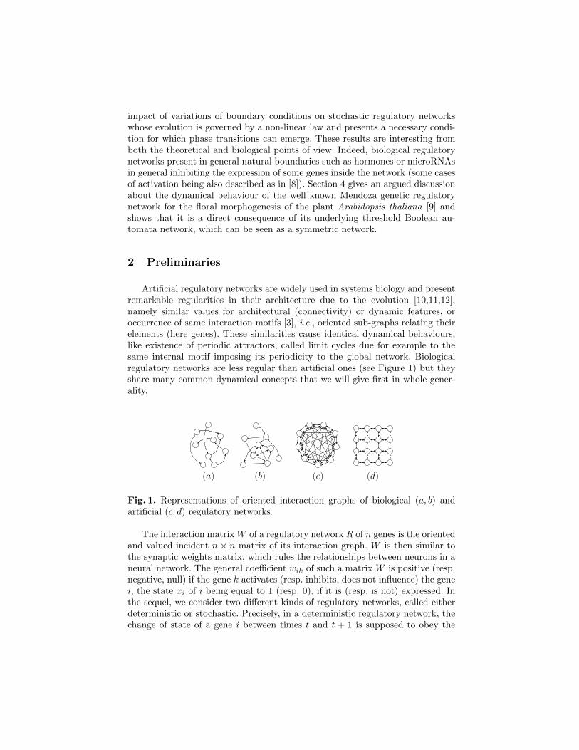
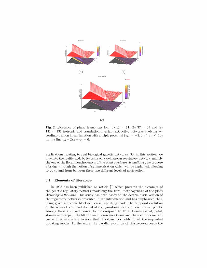
Fig. 2. Existence of phase transitions for: (a) 11 × 11, (b) 37 × 37 and (c)131 × 131 isotropic and translation-invariant attractive networks evolving ac-cording to a non linear function with a triple potential (u0 = −3, 0 ≤ u1 ≤ 10)on the line u0 + 2u1 + u2 = 0.

applications relating to real biological genetic networks. So, in this section, wedive into the reality and, by focusing on a well known regulatory network, namelythe one of the floral morphogenesis of the plant Arabidopsis thaliana , we proposea bridge, through the notion of symmetrisation which will be explained, allowingto go to and from between these two different levels of abstraction.

4.1 Elements of literature

In 1998 has been published an article [9] which presents the dynamics ofthe genetic regulatory network modelling the floral morphogenesis of the plantArabidopsis thaliana. This study has been based on the deterministic version ofthe regulatory networks presented in the introduction and has emphasised that,being given a specific block-sequential updating mode, the temporal evolutionof the network can lead its initial configurations to six different fixed points.Among these six fixed points, four correspond to floral tissues (sepal, petal,stamen and carpel), the fifth to an inflorescence tissue and the sixth to a mutanttissue. It is interesting to note that this dynamics holds for all the sequentialupdating modes. Furthermore, the parallel evolution of this network leads the

configurations to be attracted not only by these six fixed points but also by sevenlimit cycles of period two whose biological meaning is not actually known at thistime.

This observation is of particular interest because some theoretical results,given by Goles in [19], show that particular deterministic threshold Booleanautomata networks get these specific properties, as stated by the two followingtheorems:

Theorem 1. [20] If the interaction matrix W of a threshold Boolean automatanetwork is symmetric, then the period of the attractors is less or equal to 2.

Theorem 2. [21] If the interaction matrix W of a threshold Boolean automatanetwork is symmetric and such that its diagonal contains only positive coeffi-cients, then the period of the attractors equals 1 for a sequential dynamics.

4.2 The Mendoza network as a symmetric network

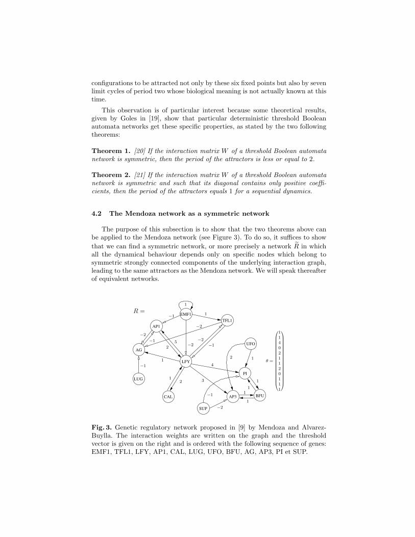
The purpose of this subsection is to show that the two theorems above canbe applied to the Mendoza network (see Figure 3). To do so, it suffices to show

that we can find a symmetric network, or more precisely a network R in whichall the dynamical behaviour depends only on specific nodes which belong tosymmetric strongly connected components of the underlying interaction graph,leading to the same attractors as the Mendoza network. We will speak thereafterof equivalent networks.

EMF1

TFL1

LFY

AG

AP1

AP3

UFO

CAL

SUP

PI

LUG

BFU

1

1

−2−2 −12

1

−1 5

−1

2 1

1

−2

1

−2

−1

3

2

11

−2

−1

1

4θ =

114021120111

R =

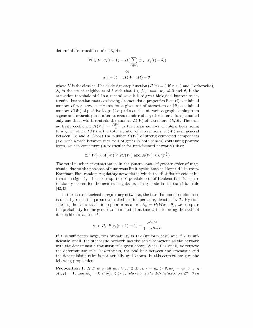
Fig. 3. Genetic regulatory network proposed in [9] by Mendoza and Alvarez-Buylla. The interaction weights are written on the graph and the thresholdvector is given on the right and is ordered with the following sequence of genes:EMF1, TFL1, LFY, AP1, CAL, LUG, UFO, BFU, AG, AP3, PI et SUP.

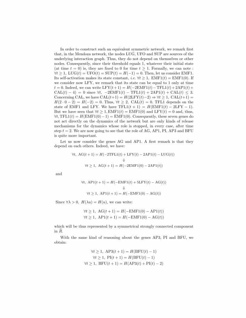
In order to construct such an equivalent symmetric network, we remark firstthat, in the Mendoza network, the nodes LUG, UFO and SUP are sources of theunderlying interaction graph. Thus, they do not depend on themselves or othernodes. Consequently, since their threshold equals 1, whatever their initial state(at time t = 0) is, they are fixed to 0 for time t ≥ 1. Formally, we can note :∀t ≥ 1, LUG(t) = UFO(t) = SUP(t) = H(−1) = 0. Then, let us consider EMF1.Its self-activation makes its state constant, i.e. ∀t ≥ 1, EMF1(t) = EMF1(0). Ifwe consider now LFY, we remark that its state can be equal to 1 only at timet = 0. Indeed, we can write LFY(t+1) = H(−2EMF1(t)−TFL1(t)+2AP1(t)+CAL(t) − 4) = 0 since ∀t, −2EMF1(t) − TFL1(t) + 2AP1(t) + CAL(t) ≤ 3.Concerning CAL, we have CAL(t+1) = H(2LFY(t)−2)⇒ ∀t ≥ 1, CAL(t+1) =H(2 · 0 − 2) = H(−2) = 0. Thus, ∀t ≥ 2, CAL(t) = 0. TFL1 depends on thestate of EMF1 and LFY. We have TFL1(t + 1) = H(EMF1(t) − 2LFY − 1).But we have seen that ∀t ≥ 1,EMF1(t) = EMF1(0) and LFY(t) = 0 and, thus,∀t,TFL1(t) = H(EMF1(0)−1) = EMF1(0). Consequently, these seven genes donot act directly on the dynamics of the network but are only kinds of releasemechanisms for the dynamics whose role is stopped, in every case, after timestep t = 2. We are now going to see that the role of AG, AP1, PI, AP3 and BFUis quite more important.

Let us now consider the genes AG and AP1. A first remark is that theydepend on each others. Indeed, we have:

∀t, AG(t + 1) = H(−2TFL1(t) + LFY(t)− 2AP1(t)− LUG(t))

⇓∀t ≥ 1, AG(t + 1) = H(−2EMF1(0)− 2AP1(t))

and

∀t, AP1(t + 1) = H(−EMF1(t) + 5LFY(t)−AG(t))

⇓∀t ≥ 1, AP1(t + 1) = H(−EMF1(0)−AG(t))

Since ∀λ > 0, H(λu) = H(u), we can write:

∀t ≥ 1, AG(t+ 1) = H(−EMF1(0)−AP1(t))

∀t ≥ 1, AP1(t+ 1) = H(−EMF1(0)−AG(t))

which will be thus represented by a symmetrical strongly connected componentin R.

With the same kind of reasoning about the genes AP3, PI and BFU, weobtain:

∀t ≥ 1, AP3(t+ 1) = H(BFU(t)− 1)

∀t ≥ 1, PI(t+ 1) = H(BFU(t)− 1)

∀t ≥ 1, BFU(t+ 1) = H(AP3(t) + PI(t)− 2)

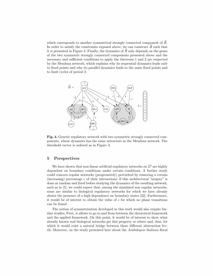
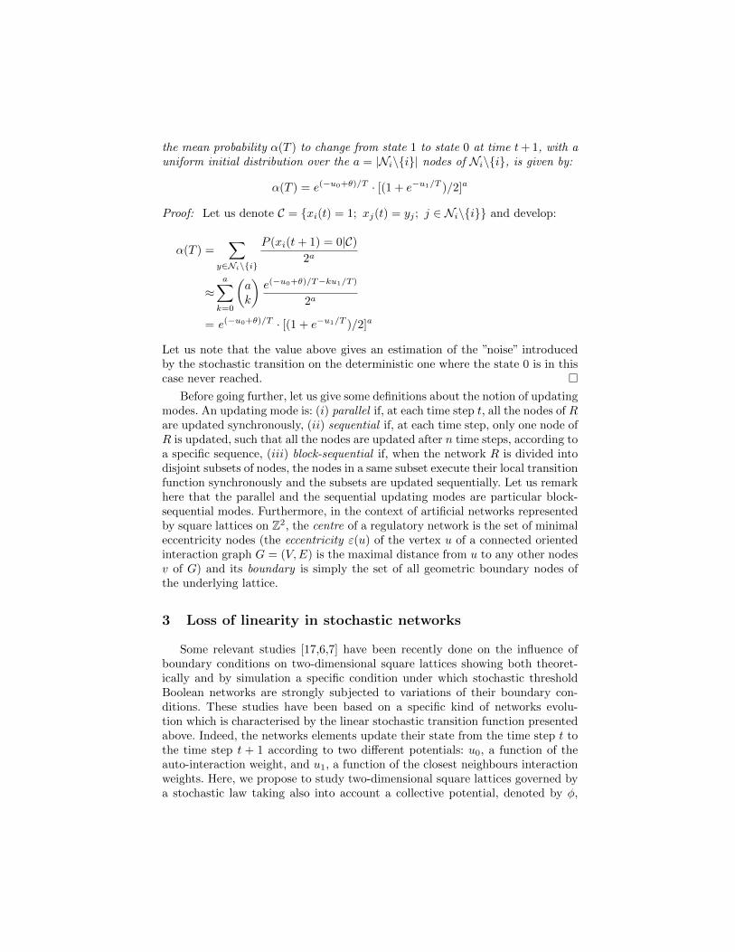
which corresponds to another symmetrical strongly connected component of R.In order to satisfy the constraints exposed above, we can construct R such thatit is presented in Figure 4. Finally, the dynamics of R only depends on the genesof the two symmetric strongly connected components presented above and thenecessary and sufficient conditions to apply the theorems 1 and 2 are respectedby the Mendoza network, which explains why its sequential dynamics leads onlyto fixed points and why its parallel dynamics leads to the same fixed points andto limit cycles of period 2.

CAL

UFO

LUG

AG AP1 TFL1 AP3 PI

BFU

SUPLFY

EMF1

4−1

1 1 1 1

− 12

−1

−1

−1

5

−1

−2

1

1

2 3

−1

1 −2 2

θ =

111021120111

− 12

R =

Fig. 4. Genetic regulatory network with two symmetric strongly connected com-ponents, whose dynamics has the same attractors as the Mendoza network. Thethreshold vector is ordered as in Figure 3.

5 Perspectives

We have shown that non-linear artificial regulatory networks on Z2 are highlydependent on boundary conditions under certain conditions. A further studycould concern regular networks (progressively) perturbed by removing a certain(increasing) percentage ε of their interactions: if this architectural ”surgery” isdone at random and fixed before studying the dynamics of the resulting network,such as in [5], we could expect that, among the simulated non regular networks,some are similar to biological regulatory networks for which we have alreadyshown the presence of a high dependence on boundary states [22]. Furthermore,it would be of interest to obtain the value of ε for which no phase transitionscan be found.

The notion of symmetrisation developed in this work would also require fur-ther studies. First, it allows to go to and from between the theoretical frameworkand the applied framework. On this point, it would be of interest to show whatalready known real biological networks get this property or others and, thus, forwhich it would exist a natural bridge between these different abstraction lev-els. Moreover, on the study presented here about the Arabidopsis thaliana floral

morphogenesis regulatory network, the fact that it is symmetric is importantbecause for symmetric threshold Boolean automata networks, one may define anenergy function on the dynamics and, then, attractors (fixed points and limitcycles) are energy’s local minima. This will give an enlarged regard on this floralmorphogenesis model.

Acknowledgements

This work has been supported in part by Eric Goles project Fondecyt 1070022;BASAL CMM and PROJECT STIC SUD.

References

1. Albert, R., Barabasi, A.L.: Statistical Mechanics of Complex Networks. Reviewsof Modern Physics 74 (2002) 47–97

2. Kitano, H.: Biological robustness. Nature Reviews Genetics 5 (2004) 826–8373. Elena, A., Demongeot, J.: Interaction Motifs in Regulatory Networks and Struc-

tural Robustness. In: Proceedings of the Second International Conference on Com-plex, Intelligent and Software Intensive Systems, IEEE Press (2008) 682–686

4. Goles, E., Salinas, L.: Comparison between Parallel and Serial Dynamics of BooleanNetworks. Theoretical Computer Science 396 (2008) 247–253

5. Fates, N., Morvan, M.: Perturbing the Topology of the Game of Life IncreasesIts Robustness to Asynchrony. In: Cellular Automata. Volume 3305 of LNCS.,Springer (2004) 111–120

6. Demongeot, J., Sene, S.: Boundary Conditions and Phase Transitions in NeuralNetworks. Simulation Results. Neural Networks 21 (2008) 962–970

7. Sene, S.: Influence des conditions de bords dans les reseaux d’automates booleens aseuil et application a la biologie. PhD thesis, Universite Joseph Fourier de Grenoble(2008)

8. Jopling, C.L., Yi, M., Lancaster, A.M., Lemon, S.M., Sarnow, P.: Modulation ofHepatitis C Virus RNA Abundance by a Liver-Specific MicroRNA. Science 309(2005) 1577–1581

9. Mendoza, L., Alvarez-Buylla, E.R.: Dynamics of the Genetic Regulatory Networkfor Arabidopsis thaliana Flower Morphogenesis. Journal of Theoretical Biology193 (1998) 307–319

10. de Duve, C.: Life Evolving. Oxford University Press (2002)11. Eigen, M., Gardiner, W., Schuster, P., Winkler-Oswatitsch, R.: The Origin of

Genetic Information. Scientific American 244 (1981) 88–9212. Gardner, M.: Mathematical Games. The Fantastic Combinations of John Conway’s

New Solitaire Game ”Life”. Scientific American 223 (1970) 20–12313. Hopfield, J.J.: Neural Networks and Physical Systems with Emergent Collective

Computational Abilities. Proceedings of the National Academy of Science of theUSA 79 (1982) 2554–2558

14. McCulloch, W.S., Pitts, W.: A Logical Calculus of the Ideas Immanent in NervousActivity. Journal of Mathematical Biology 5 (1943) 115–133

15. Cinquin, O., Demongeot, J.: Positive and Negative Feedback: Striking a BalanceBetween Necessary Antagonists. Journal of Theoretical Biology 216 (2002) 229–241

16. Kaufman, M., Soule, C., Thomas, R.: A New Necessary Condition on InteractionGraphs for Multistationarity. Journal of Theoretical Biology 248 (2007) 675–685

17. Demongeot, J., Jezequel, C., Sene, S.: Boundary Conditions and Phase Transitionsin Neural Networks. Theoretical Results. Neural Networks 21 (2008) 971–979

18. Dobrushin, R.L.: The Problem of Uniqueness of a Gibbsian Random Field and theProblem of Phase Transitions. Functional Analysis and Its Applications (1968)

19. Goles, E., Martinez, S.: Neural and Automata Networks. Kluwer Academic Pub-lishers (1990)

20. Goles, E., Olivos, J.: Comportement periodique des fonctions seuils binaires etapplications. Discrete Applied Mathematics 3 (1981) 93–105

21. Fogelman-Soulie, F., Goles, E., Weisbuch, G.: Transient Length in SequentialIteration of Threshold Functions. Discrete Applied Mathematics 6 (1983) 95–98

22. Ben Amor, H., Demongeot, J., Sene, S.: Structural Sensitivity of Neural and Ge-netic Networks. In: MICAI. Volume 5317 of Lecture Notes in Computer Science.,Springer (2008) 973–986