Graph-theoretic description of the interplay between non-linearity and connectivity in biological...

Graph-theoretic description of the interplaybetween non-linearity and connectivity in

biological systems

R. D�õaz-Sierra 1, B. Hern�andez-Bermejo 2, V. Fair�en *

Departamento de F�õsica Fundamental, Universidad Nacional de Educaci�on a Distancia, Apartado

60141, 28080 Madrid, Spain

Received 15 March 1998; accepted 7 April 1998

Abstract

The purpose of this article is to stress the implications that the consideration of non-

linearity has upon the extension and strength of connectivity, if this is understood as a

characterization of the degree of interrelation between parts of the system. This ob-

jective is reached within the QP formalism for non-linear ODEs. The formalism is de-

veloped in a graph-theoretic setting, with the help of which the connectionist aspect of

non-linearity becomes apparent. Topology-preserving transformations involve an ex-

change between the degree of non-linearity and the strengths of interactions, thus as-

sembling systems of apparently di�erent nature into classes of equivalence. We argue

that, if we have in mind a classi®cation of systems according to behavior, these classes of

equivalence should be given their proper singularity. We characterize globally the

connectivity of a class with an index, although we point out during the discussion that

the mathematical conception of the complex idea of connectivity is still incom-

plete. Ó 1999 Elsevier Science Inc. All rights reserved.

Keywords: Graph theory; Connectivity; Non-linearity; Generalized Lotka±Volterra

equations; QP-formalism for ODEs

Mathematical Biosciences 156 (1999) 229±253

* Corresponding author. Fax: +34-1 398 6697; e-mail: [email protected] E-mail: [email protected] E-mail: [email protected].

0025-5564/99/$ ± see front matter Ó 1999 Elsevier Science Inc. All rights reserved.

PII: S 0 0 2 5 - 5 5 6 4 ( 9 8 ) 1 0 0 6 8 - 8

1. Introduction

This paper is about connectionism, or more precisely, about connectionistrepresentations ± or models ± of biological systems. A connectionist model issimply an abstraction in which the system is regarded as a set of elementaryunits which are connected together to form a network [1]; the metaphor beingparticularly popular in biology, especially in studies in theoretical populationbiology [2], or in catalytic [1,3,4] and immune nets [1]. Details of the underlyingcommon mathematical structure will be elaborated upon later, but what isimportant here is to realize that a common denominator to most conventionalconnectionist models is to view them as `®xed' in form. The variability is thenwholly encapsulated in the state of the vertices (or nodes), the transition rule ofwhich is usually speci®ed by ordinary di�erential equations or discrete timemaps. The connections are ®xed and their strengths are taken in their simplestpossible representation, that is, in terms of the constant values of the entries ofa matrix. In the ®eld of population dynamics, for example, networks are thenan iconic representation of structurally simple dynamical systems ± linear,general Lotka±Volterra, or equivalently, replicator ± , in which a speci®cconnectivity pattern is given a particular emphasis in the establishment of re-lations between the expected qualitative behavior and certain structuralproperties of the net [5±13]. This approach disregards the proper functionalform of interactions, which is collapsed into the simplest possible mathematicalexpression. Generic qualitative features such as the amount, distribution andsign of internal connections, occupy instead the pivotal position in supportingconjectures in such important theoretical issues as those concerning, for ex-ample, the complexity vs. stability debate in ecological modeling [14±19].

The e�ect of interactions with a high degree of non-linearity has not beenalways eluded. It has however been restricted to models with very few vari-ables, solved case to case, outside the context of any connectionist frameworkwhatsoever. The reason seems to be quite simple. As soon as we depart fromthe structurally simple models used in the connectionist approach describedabove, connection strengths depend upon, and vary with, the states of thesystem. And, they may do so in very di�erent ways. This makes models to berepresentation-dependent, a fact which does not facilitate the inclusion of ar-bitrary non-linearities within a tentative connectionist description. Thus, theabsence of a proper framework has dismissed such inquiries as, for example,the investigation on how holling type rate laws might a�ect a stability vs.connectance, or vs. number of species relationship.

It is intended here to show that it is perfectly possible to o�er a mathe-matical scheme where non-linearity can be reconciled with a connectivist pointof view. By elaborating on an appropriate universal format of the evolutionequations written in terms of combinations of rates in power law form, we shalldiscover how the concepts of connectivity and non-linearity are closely inter-

230 R. D�õaz-Sierra et al. / Mathematical Biosciences 156 (1999) 229±253

mingled and cannot be examined separately. Operations in the connectionstrengths a�ect the connective architecture of a network of interacting entities,the reciprocal being also true. The result is that connectivity in a network lossesits meaning if no reference is made to the degree of non-linearity, and viceversa. The consequence is that the interplay between both facets of a systemdisrupts the traditional association between a given level of connectance and anexpected behavior. Instead, we ®nd the ensemble of would-be models parti-tioned into classes of equivalence. The members of a given class do di�er intheir degrees of connectance and non-linearity, but share the same globalqualitative behavior. Within a class, models are related one to each otherthrough topology preserving transformations. The latter leave invariant agiven product of two matrices, the entries of which are the connection strengthsand the degrees of non-linearity, respectively. This invariant product mightthus be considered a potential candidate substitute for the traditional conceptof community matrix [6] as the meaningful mathematical object to be con-sidered in the search for a potential classi®cation of models according to ex-pected behavior.

The framework in which we will operate is the quasipolynomial (QP) for-malism [20±29]. We demonstrated in previous publications [25±27] how verygeneral systems represented in terms of ordinary di�erential equations, can beencapsulated within this formal scheme. Although all the aforementionedfeatures can be formulated algebraically, we shall here adopt essentially a con-nectionist point of view, without neglecting to resort to some algebraic manipula-tions whenever found necessary for the sake of clarity in the exposition.

The foundation of a connectionist representation is a graph consisting ofnodes (vertices) and connections (links, edges, or arcs) between them. So, weshall reason in terms of graphs. Graphs will be of two types. On the one hand,we shall introduce the rather conventional digraph, where the representation ofnon-linearity on connections is not easy to visualize and operate with. This willlead us to the introduction of a more appropriate and workable diagram ±somehow reminiscent of bipartite graphs [30] ± which will become our workingmodel throughout the paper.

This work has an important consequence. We emphasize here why theconcept of connectivity should be reconsidered. Till now it has been essentiallyhandled in the context of linear di�erential systems and has not raised im-portant conceptual questions. We point out how both, the coming into actionof non-linearity, and the connectionist description, open new possibilities ofthought on the concept of connectivity. The idea of class of equivalence ofsystems sharing the same behavior, casts a new light on the possible relationconnectivity-behavior, and thus sets up limits on the appropriateness of thetraditional de®nition. A connectivity should be associated to both an indi-vidual system and to a class of equivalence. We make a ®rst step in this di-rection by suggesting the de®nition of an index of the class.

R. D�õaz-Sierra et al. / Mathematical Biosciences 156 (1999) 229±253 231

The paper starts with a review of the algebraic properties of the QP-for-malism. In Section 3, we de®ne its connectionist representation, and in Sec-tion 4 we elaborate on some of its implications. It is here where we characterizeconnectivity index. Finally, Section 5 is devoted to the conclusions.

2. Algebraic preliminaries on the QP formalism

2.1. Non-linear theory

The quasipolynomial (QP) format for ODEs [20±29] is given by

_xi � xi ki

�Xm

j�1

Aij

Yn

k�1

xBjkk

!; i � 1; . . . ; n; �2:1�

where n and m are positive integers, and A, B and k are n� m, m� n and n� 1real matrices, respectively, and which are assumed to be of maximal rank. Weshall also assume m P n. As it can be demonstrated [28], every QP-system notcomplying to these requirements can be reduced to this standard case. Some-times it will also be convenient to consider the n� �m� 1� composite matrixM � �kjA�:

We shall in this section review brie¯y some algebraic properties of the for-malism associated to Eq. (2.1). By a rather simple process very general systemscan be brought under this formalism, whatever the type of non-linearity is[25±27]. For the sake of notation, n will always denote the number of variablesof a QP-system, and m the number of per capita rates (PCRs from now on):Yn

k�1

xBjkk ; j � 1; . . . ;m: �2:2�

The pivotal property of system Eq. (2.1) is that of being formally invariantunder quasimonomial transformations [20,21], de®ned as

xi �Yn

k�1

yCikk ; i � 1; . . . ; n; �2:3�

for any invertible real matrix C. Under Eq. (2.3), matrices B, A, k and Mchange to

B0 � B � C; A0 � Cÿ1 � A; k0 � Cÿ1 � k; M 0 � Cÿ1 �M ; �2:4�respectively, and all QP-systems which can be connected through quasimo-nomial transformations share the value of the product B �M , and constitute aclass of equivalence. The m PCRs in Eq. (2.1), when considered as functions oftime, are also invariants of the class and the solutions to all the members of aclass are topologically equivalent [25]. Conversely, two di�erent classes cannothave the same B �M product, as the following theorem shows:


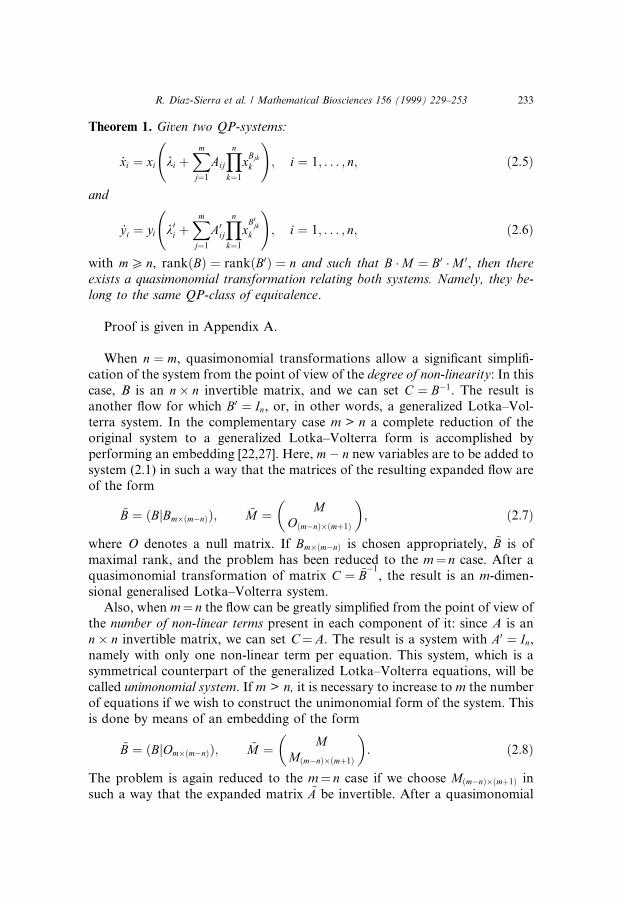
Theorem 1. Given two QP-systems:

_xi � xi ki

�Xm

j�1

Aij

Yn

k�1

xBjkk

!; i � 1; . . . ; n; �2:5�

and

_yi � yi k0i

�Xm

j�1

A0ijYn

k�1

xB0jkk

!; i � 1; . . . ; n; �2:6�

with m P n, rank�B� � rank�B0� � n and such that B �M � B0 �M 0, then thereexists a quasimonomial transformation relating both systems. Namely, they be-long to the same QP-class of equivalence.

Proof is given in Appendix A.

When n � m, quasimonomial transformations allow a signi®cant simpli®-cation of the system from the point of view of the degree of non-linearity: In thiscase, B is an n� n invertible matrix, and we can set C � Bÿ1. The result isanother ¯ow for which B0 � In, or, in other words, a generalized Lotka±Vol-terra system. In the complementary case m > n a complete reduction of theoriginal system to a generalized Lotka±Volterra form is accomplished byperforming an embedding [22,27]. Here, mÿ n new variables are to be added tosystem (2.1) in such a way that the matrices of the resulting expanded ¯ow areof the form

~B � �BjBm��mÿn��; ~M � MO�mÿn��m�1�

� �; �2:7�

where O denotes a null matrix. If Bm��mÿn� is chosen appropriately, ~B is ofmaximal rank, and the problem has been reduced to the m� n case. After aquasimonomial transformation of matrix C � ~B

ÿ1, the result is an m-dimen-

sional generalised Lotka±Volterra system.Also, when m� n the ¯ow can be greatly simpli®ed from the point of view of

the number of non-linear terms present in each component of it: since A is ann� n invertible matrix, we can set C�A. The result is a system with A0 � In,namely with only one non-linear term per equation. This system, which is asymmetrical counterpart of the generalized Lotka±Volterra equations, will becalled unimonomial system. If m > n, it is necessary to increase to m the numberof equations if we wish to construct the unimonomial form of the system. Thisis done by means of an embedding of the form

~B � �BjOm��mÿn��; ~M � MM�mÿn��m�1�

� �: �2:8�

The problem is again reduced to the m� n case if we choose M�mÿn��m�1� insuch a way that the expanded matrix ~A be invertible. After a quasimonomial


transformation of matrix C � ~A, we arrive at an m-dimensional unimonomialsystem.

The quasimonomial transformations are complemented by new-timetransformations of the form [29]

dt �Yn

i�1

xbii

!dt0; �2:9�

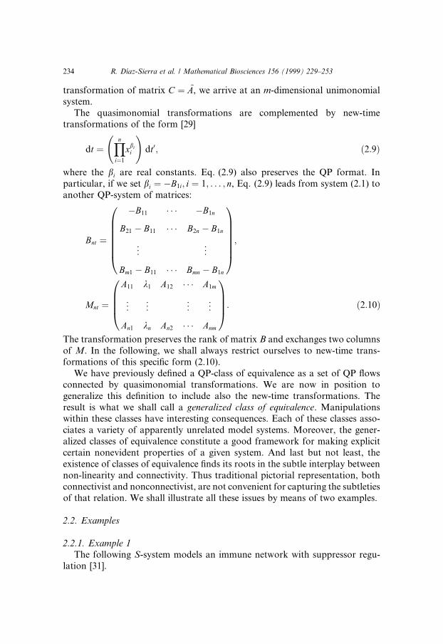
where the bi are real constants. Eq. (2.9) also preserves the QP format. Inparticular, if we set bi � ÿB1i; i � 1; . . . ; n, Eq. (2.9) leads from system (2.1) toanother QP-system of matrices:

Bnt �

ÿB11 � � � ÿB1n

B21 ÿ B11 � � � B2n ÿ B1n

..

. ...

Bm1 ÿ B11 � � � Bmn ÿ B1n

0BBBBBB@

1CCCCCCA;

Mnt �

A11 k1 A12 � � � A1m

..

. ... ..

. ...

An1 kn An2 � � � Anm

0BBB@1CCCA: �2:10�

The transformation preserves the rank of matrix B and exchanges two columnsof M. In the following, we shall always restrict ourselves to new-time trans-formations of this speci®c form (2.10).

We have previously de®ned a QP-class of equivalence as a set of QP ¯owsconnected by quasimonomial transformations. We are now in position togeneralize this de®nition to include also the new-time transformations. Theresult is what we shall call a generalized class of equivalence. Manipulationswithin these classes have interesting consequences. Each of these classes asso-ciates a variety of apparently unrelated model systems. Moreover, the gener-alized classes of equivalence constitute a good framework for making explicitcertain nonevident properties of a given system. And last but not least, theexistence of classes of equivalence ®nds its roots in the subtle interplay betweennon-linearity and connectivity. Thus traditional pictorial representation, bothconnectivist and nonconnectivist, are not convenient for capturing the subtletiesof that relation. We shall illustrate all these issues by means of two examples.

2.2. Examples

2.2.1. Example 1The following S-system models an immune network with suppressor regu-

lation [31].


_x1 � 8x1 ÿ 8x1x1=22 ;

_x2 � x1=21 xÿ1=2

3 ÿ x2;

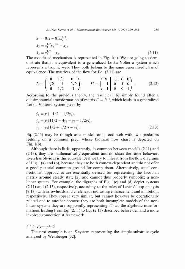
_x3 � x1=22 ÿ x3: �2:11�

The associated mechanism is represented in Fig. 1(a). We are going to dem-onstrate that it is equivalent to a generalized Lotka±Volterra system whichrepresents a trophic web. They both belong to the same generalized class ofequivalence. The matrices of the ¯ow for Eq. (2.11) are

�2:12�

According to the previous theory, the result can be simply found after aquasimonomial transformation of matrix C � Bÿ1, which leads to a generalizedLotka±Volterra system given by

_y1 � y1�ÿ1=2� 1=2y2�;_y2 � y2�11=2ÿ 4y1 ÿ y2 ÿ 1=2y3�;_y3 � y3�1=2� 1=2y2 ÿ y3�: �2:13�

Eq. (2.13) may be though as a model for a food web with two predatorsfeelding on a common prey, whose biomass ¯ow chart is depicted onFig. 1(b).

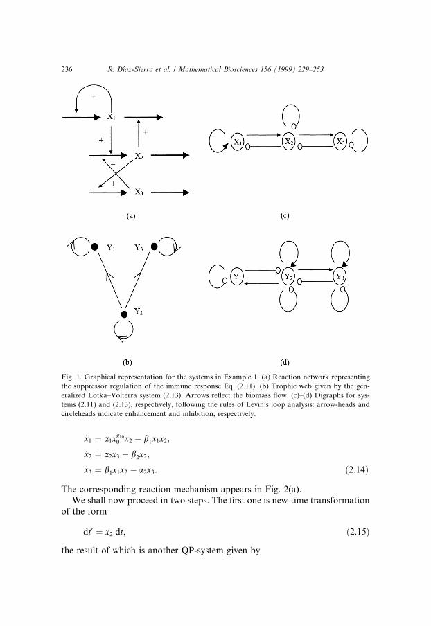
Although there is little, apparently, in common between models (2.11) and(2.13), they are mathematically equivalent and do share the same behavior.Even less obvious is this equivalence if we try to infer it from the ¯ow diagramsof Fig. 1(a) and (b), because they are both context-dependent and do not o�era good pictorial common ground for comparison. Alternatively, usual con-nectionist approaches are essentially devised for representing the Jacobianmatrix around steady state [2], and cannot thus properly symbolize a non-linear system. For example, the digraphs of Fig. 1(c) and (d) depict systems(2.11) and (2.13), respectively, according to the rules of Levins' loop analysis[9,13], with arrowheads and circleheads indicating enhancement and inhibition,respectively. They appear very similar, but cannot however be operationallyrelated one to another because they are both incomplete models of the non-linear systems they are supposedly representing. Thus, the algebraic transfor-mations leading from Eq. (2.11) to Eq. (2.13) described before demand a moreinvolved connectionist framework.

2.2.2. Example 2The next example is an S-system representing the simple substrate cycle

analyzed by Weinberger [32].


_x1 � a1xg10

0 x2 ÿ b1x1x2;

_x2 � a2x3 ÿ b2x2;

_x3 � b1x1x2 ÿ a2x3: �2:14�The corresponding reaction mechanism appears in Fig. 2(a).

We shall now proceed in two steps. The ®rst one is new-time transformationof the form

dt0 � x2 dt; �2:15�the result of which is another QP-system given by

Fig. 1. Graphical representation for the systems in Example 1. (a) Reaction network representing

the suppressor regulation of the immune response Eq. (2.11). (b) Trophic web given by the gen-

eralized Lotka±Volterra system (2.13). Arrows re¯ect the biomass ¯ow. (c)±(d) Digraphs for sys-

tems (2.11) and (2.13), respectively, following the rules of Levin's loop analysis: arrow-heads and

circleheads indicate enhancement and inhibition, respectively.


�2:16�

The second step proceeds to a quasimonomial transformation upon Eq. (2.16)with matrix

C �1 0 00 ÿ1 00 0 1

0@ 1A; �2:17�

after which we ®nd the target system:

_y1 � a1xg10

0 ÿ b1y1;

_y2 � b2y22 ÿ a2y3

2y3;

_y3 � b1y1 ÿ a2y2y3: �2:18�

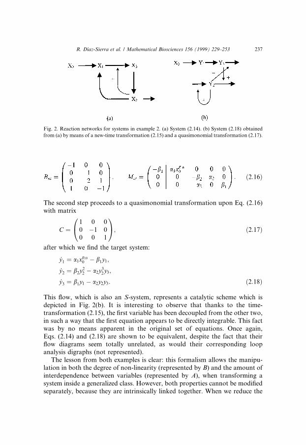
This ¯ow, which is also an S-system, represents a catalytic scheme which isdepicted in Fig. 2(b). It is interesting to observe that thanks to the time-transformation (2.15), the ®rst variable has been decoupled from the other two,in such a way that the ®rst equation appears to be directly integrable. This factwas by no means apparent in the original set of equations. Once again,Eqs. (2.14) and (2.18) are shown to be equivalent, despite the fact that their¯ow diagrams seem totally unrelated, as would their corresponding loopanalysis digraphs (not represented).

The lesson from both examples is clear: this formalism allows the manipu-lation in both the degree of non-linearity (represented by B) and the amount ofinterdependence between variables (represented by A), when transforming asystem inside a generalized class. However, both properties cannot be modi®edseparately, because they are intrinsically linked together. When we reduce the

Fig. 2. Reaction networks for systems in example 2. (a) System (2.14). (b) System (2.18) obtained

from (a) by means of a new-time transformation (2.15) and a quasimonomial transformation (2.17).


degree of non-linearity, as in the generalized Lotka±Volterra form (see example 1)we loose control over the number and distribution of links among variables±over connectance, in other words. The converse is true for unimonomial form.They are two facets of the same reality, each of them being amenable totransformation into the other. This consideration is unavoidable if we wish togeneralize the concept of connectance into the non-linear world. This will beour aim in the rest of this work.

2.3. Linear theory

The QP format is also a suitable tool for the study of the linearized systemaround a ®xed point. The Jacobian can be easily expressed in terms of itsmatrices, A and B, and the values of the ®xed point. To a quasimonomialtransformation between two QP-system, the theory assigns a similarity trans-formation between its corresponding Jacobians. A relation is thus established,which maps a QP-class of equivalence into a class of linear systems relatedthrough linear transformations. The forthcoming two theorems and a corollarydevelop these properties.

Theorem 2. Let be a QP-system and one of its ®xed points, arranged as a columnvector xs, and de®ne another column vector, q, for the values taken by the PCRsat this ®xed point. Then, its Jacobian, or community matrix, at this ®xed pointcan simply be expressed as a matrix product

J � Xs � A � Q � B � Xÿ1s ; �2:19�

where Xs and Q are diagonal matrices such that �Xs�ii � xs;i and Qii � qi.

Proof is given in Appendix A.

Theorem 3. Let be two QP-systems and their matrices at a ®xed point:�A1;B1;Xs; J1� and �A2;B2; Ys; J2�. If both QP-systems belong to the same class ofequivalence, that is, if they are related by a quasimonomial transformation

A2 � Cÿ1 � A1 B2 � B1 � C ys;i �Yn

k�1

x�Cÿ1�ik

s;k ; �2:20�

then their linearizations are related by a linear transformation:

J2 � L � J1 � Lÿ1; �2:21�where L is given by the following matrix product:

L � Ys � Cÿ1 � Xÿ1s : �2:22�

Proof is given in Appendix A.From this theorem we can conclude an interesting result:


Corollary 1. All the linearizations of QP-systems belonging to the same QP classof equivalence, when de®ned at the same ®xed point, have the same spectrum ofeigenvalues.

3. Basis for a connectionist description of non-linear systems

3.1. Simple graphs

The simplest graph representation in biology [2,8] involves points, or nodes,representing the variables of the system. Arcs connecting nodes depict themutual in¯uences of these variables among themselves. These graphs arewidely used in systems characterized by a single matrix, like in linear or gen-eralized Lotka±Volterra systems. For example, in the latter case each PCR isequal to one variable, then variables in¯uence each other directly, and a simplearc with constant weight is enough to characterize them.

However, the non-linearity in a system in QP format requires a more in-volved de®nition of connections. They will take the form of compound arrows(see Fig. 3(a)). There will be one of these compound arrows per PCR in thesystem, and it should carry information about variables form this PCR andwhich ones it modi®es through the equations of evolution. The main compo-nent of this arrow is the body, a single thick arc, with multiple heads and tails.The tails are arcs connecting one end of the arrowbody to the variables nodesentering the PCR. The heads are simple arrows beginning at the other end ofthe body, and pointing to those variables nodes which are modi®ed by thePCR. We can also represent the sign of the linear term ki in Eq. (2.1): the nodewill be white if ki � 0, doted if ki > 0 and with gray lines if ki < 0.

We have now de®ned that basic tools for building up the arquitecture of theQP-graph. To complete the description we can add weights to the arrows. Atan arrowtail we write the variable's exponent in the PCR; that is, the arcjoining the jth PCRs body to the kth node has a weight equal to Bjk. The ar-rowhead will have weights given by the constant multiplying the PCR in theequations. So, we write the value Aij in the arrow going from the jth PCRs bodyto the ith node. Fig. 3(a) represents the graph for system (2.11).

We have de®ned an oriented weighted graph for system (2.1), which we shallcall simple graph. We can already guess from it how the system's non-linearitymakes the structure more complex and imprints on its connectivity. However,even though these graphs are closely related to the standard graphs in use inconnectivity vs. stability studies, they are not appropriate for exploiting thepower of the QP formalism. The transformations between systems, de®ned inSection 2, become involved and the interesting inferences from the manipula-tion of these graphs are hardly visualized. We introduce next an alternativerepresentation for QP-graphs, equivalent to the previous one, but on which allthe consequences of the algebraic formalism will become straightforward.


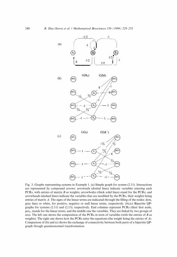
Fig. 3. Graphs representing systems in Example 1. (a) Simple graph for system (2.11). Interactions

are represented by compound arrows: arrowtails (dotted lines) indicate variables entering each

PCRs, with entries of matrix B as weights; arrowbodys (thick solid lines) stand for the PCRs; and

arrowheads (dashed lines) indicate the variables that are modi®ed by the PCRs, their weights being

entries of matrix A. The signs of the linear terms are indicated through the ®lling of the nodes: dots,

gray lines or white, for positive, negative or null linear terms, respectively. (b),(c) Bipartite QP-

graphs for systems (2.11) and (2.13), respectively. End columns represent PCRs (their ®rst node,

pcr0, stands for the linear term), and the middle one the variables. They are linked by two groups of

arcs. The left one shows the composition of the PCRs in term of variables (with the entries of B as

weights). The right one shows how the PCRs enter the equations (the weight being the entries of A).

Comparison of (b) and (c) shows the exchange of connectivity between both parts of a bipartite QP-

graph though quasimonomial transformation.


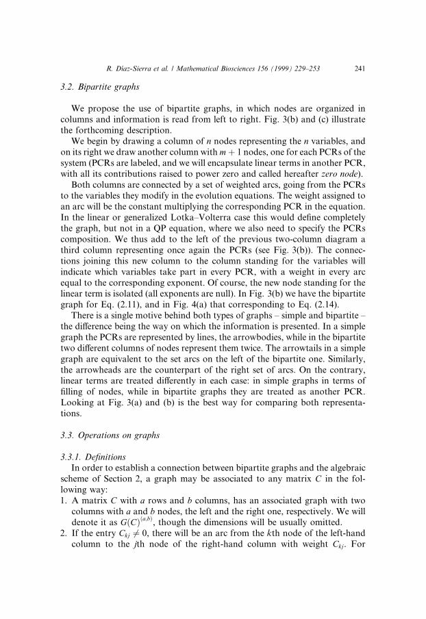
3.2. Bipartite graphs

We propose the use of bipartite graphs, in which nodes are organized incolumns and information is read from left to right. Fig. 3(b) and (c) illustratethe forthcoming description.

We begin by drawing a column of n nodes representing the n variables, andon its right we draw another column with m� 1 nodes, one for each PCRs of thesystem (PCRs are labeled, and we will encapsulate linear terms in another PCR,with all its contributions raised to power zero and called hereafter zero node).

Both columns are connected by a set of weighted arcs, going from the PCRsto the variables they modify in the evolution equations. The weight assigned toan arc will be the constant multiplying the corresponding PCR in the equation.In the linear or generalized Lotka±Volterra case this would de®ne completelythe graph, but not in a QP equation, where we also need to specify the PCRscomposition. We thus add to the left of the previous two-column diagram athird column representing once again the PCRs (see Fig. 3(b)). The connec-tions joining this new column to the column standing for the variables willindicate which variables take part in every PCR, with a weight in every arcequal to the corresponding exponent. Of course, the new node standing for thelinear term is isolated (all exponents are null). In Fig. 3(b) we have the bipartitegraph for Eq. (2.11), and in Fig. 4(a) that corresponding to Eq. (2.14).

There is a single motive behind both types of graphs ± simple and bipartite ±the di�erence being the way on which the information is presented. In a simplegraph the PCRs are represented by lines, the arrowbodies, while in the bipartitetwo di�erent columns of nodes represent them twice. The arrowtails in a simplegraph are equivalent to the set arcs on the left of the bipartite one. Similarly,the arrowheads are the counterpart of the right set of arcs. On the contrary,linear terms are treated di�erently in each case: in simple graphs in terms of®lling of nodes, while in bipartite graphs they are treated as another PCR.Looking at Fig. 3(a) and (b) is the best way for comparing both representa-tions.

3.3. Operations on graphs

3.3.1. De®nitionsIn order to establish a connection between bipartite graphs and the algebraic

scheme of Section 2, a graph may be associated to any matrix C in the fol-lowing way:1. A matrix C with a rows and b columns, has an associated graph with two

columns with a and b nodes, the left and the right one, respectively. We willdenote it as G�C��a;b�, though the dimensions will be usually omitted.

2. If the entry Ckj 6� 0, there will be an arc from the kth node of the left-handcolumn to the jth node of the right-hand column with weight Ckj. For


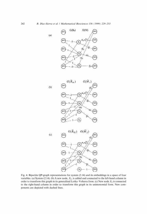
Fig. 4. Bipartite QP-graph representations for system (2.14) and its embeddings in a space of four

variables. (a) System (2.14). (b) A new node, X4, is added and connected to the left-hand column in

order to transform this graph in its generalized Lotka±Volterra form. (c) New node X4 is connected

to the right-hand column in order to transform this graph in its unimonomial form. New com-

ponents are depicted with dashed lines.


example, the graph in Fig. 3(b) can be viewed as the assembly of two graphs,G�B� and G�M� associated with matrices (2.12).

A compound graph is an assembly of two or more sequentially connected matrix

graphs, G�C1��a;b� G�C2��b;c� G�C3��c;d� . . ., ful®lling the condition that thenumber of nodes in the second column of one matrix graph is the same as thenumber of nodes in the ®rst column of the following matrix graph.

Sometimes, when found diagrammatically convenient, two adjoining col-umns with equal number of nodes may be collapsed into a single column. Thisis what happens in a bipartite graph of a QP-system which is no more than acompound graph of the graphs of matrices B and M , G�B0� G�M� asFig. 3(b), where B0 is obtained by adding matrix B a ®rst row of null entries(this meaning of the zero subscript will be maintained hereinafter).

3.3.2. Product graphWe begin with two matrix graphs, G�P1��a;b� and G�P2��b;c�. If we assemble

them in a compound graph we can easily de®ne its graph product. It is a graphG�P3��a;c� � G�P1� � G�P2�, with a and c nodes in each column, which is de®nedaccording to the following rules:1. In the compound graph, we have to look for all the possible uninterrupted

paths linking nodes on the far left column to nodes on the far right one. Twoarcs, one joining the ith node of the left-hand column to the jth node of theone on the middle, and the other from the kth node of this middle column tothe sth node on the right-hand column, form an uninterrupted path if j � k,that is to say, if the second arc begins in the node where the ®rst ends.

2. For every uninterrupted path in the compound graph G�P1� G�P2�, therewill be an arc in the product graph, G�P3�, having a weight equal to theproduct of the weights of arcs constituting the path.

3. If two more paths share common end nodes they generate a single arc,whose weight is the sum of weights of the individual paths.

For example the right hand graph G�M 0� of the compound graph G�I0� G�M 0� in Fig. 3(c), is the product of the graphs G�B� � G�M� in Fig. 3(b).

Proposition 1. Given two matrices, P1, P2, and their associated graphs, G�P1� andG�P2�, then the product graph, G�P3� � G�P1� � G�P2�, is the graph representationfor the product matrix, P3 � P1 � P2.

We can also de®ne the product of more than two graphs. We just have todraw their compound graph and look for all uninterrupted paths, now de®nedto be composed of more than two arcs. The product graph will have twocolumns of nodes and arcs joining them, with weights equal to the product ofall the arc weights forming the uninterrupted path.

It is useful to translate some well-known de®nitions in matrix theory into thegraph setting:


A. The identity graph, G�I��n;n�, multiplied by any other graph G�P�, leaves itinvariant

G�P � � G�I� � G�I� � G�P� � G�P �: �3:1�Graph G�I��n;n� has n horizontal arcs joining corresponding nodes, as can beseen at the left-hand graph of the compound graph G�I0� G�B� in Fig. 3(c).

B. The inverse graph, G�Pÿ1��n;n�, of a graph G�P ��n;n� is the one which ful®lls

G�P � � G�Pÿ1� � G�Pÿ1� � G�P � � G�I� �3:2�

3.4. Transformations on QP-graphs

We are now ready to de®ne transformations among graphs and equivalenceclasses of graphs, as we did in Section 2 for the algebraic representation.

A quasimonomial transformation (2.3) can be completely described by amatrix graph G�C�, with its ®rst column representing the old variables xi, andthe second column the new ones, yi. The product G�C� G�Cÿ1�, which isequivalent to the identity graph, can replace the central column of a QP-sys-tems bipartite graph. We have

G�B0� G�M� ! G�B0� G�C� G�Cÿ1� G�M�! �G�B0� � G�C�� G�Cÿ1� � G�M�� G�B00� G�M 0�:

The QP-system is thus reformulated in the new variables, and a correspondenceestablished with Eq. (2.4). All bipartite QP-graphs related by a quasimonomialtransformation constitute an equivalence class, with the product graph G�B0� �G�M� as a class invariant.

The canonical forms of the class can be easily built up. This is straightfor-ward in systems with m � n, which is what happens in Eq. (2.12) ± seeFig. 3(b). The generalized Lotka±Volterra canonical form of system Eq. (2.13),is represented in Fig. 3(c), and can be reached from the graph at Fig. 3(b) bychoosing G�C� � G�Bÿ1�. The degree of non-linearity has been reduced to itsminimal expression, at the expense of a substantial increase in the level ofconnectivity among variables ± compare G�M 0� with G�M�. It is the same forthe unimonomial canonical form, where G�C� � G�A�. We simplify the right-hand side of the target bipartite QP-graph to the identity except for the linearnode by getting a system with only one non-linear term per equation and whosebipartite QP-graph is �G�B� � G�A�� G�kjI�. The situation here is reversedwith respect to the previous case: we reduce the level of connectivity amongvariables, though we add complexity to the non-linearity.

We cannot proceed to the obtainment of the canonical forms m > n withoutsome prior arrangement on the bipartite QP-graph. End columns have a largernumber of nodes than the middle one, so neither side of the compound QP-graph can be transformed into the identity graph. (see Fig. 4(a)). The problem


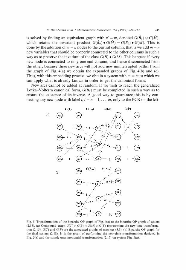
is solved by ®nding an equivalent graph with n0 � m, denoted G� ~B0� G� ~M�,which retains the invariant product G� ~B0� � G� ~M� � G�B0� � G�M�. This isdone by the addition of mÿ n nodes to the central column, that is we add mÿ nnew variables that should be properly connected to the other columns in such away as to preserve the invariant of the class G�B� � G�M�. This happens if everynew node is connected to only one end column, and hence disconnected fromthe other, because these new arcs will not add new uninterrupted paths. Fromthe graph of Fig. 4(a) we obtain the expanded graphs of Fig. 4(b) and (c).Thus, with this embedding process, we obtain a system with n0 � m to which wecan apply what is already known in order to get the canonical forms.

New arcs cannot be added at random. If we wish to reach the generalizedLotka±Volterra canonical form, G� ~B0� must be completed in such a way as toensure the existence of its inverse. A good way to guarantee this is by con-necting any new node with label i, i � n� 1; . . . ;m; only to the PCR on the left-

Fig. 5. Transformation of the bipartite QP-graph of Fig. 4(a) to the bipartite QP-graph of system

(2.18). (a) Compound graph G�T � G�B� G�M� G�T � representing the new-time transforma-

tion (2.15). G(T) and G(P) are the associated graphs of matrices (3.3). (b) Bipartite QP-graph for

the ®nal system (2.18). It is the result of performing the new-time transformation depicted in

Fig. 5(a) and the simple quasimonomial transformation (2.17) on system Fig. 4(a).


hand column with the same lable (see Fig. 4(a)). Alternatively, in the unimo-nomial canonical form we have G�C� � G� ~A�, which has an inverse only whenall new nodes are appropriately connected to the right-hand column of nodes,as in Fig. 5(b).

To conclude the transformations on bipartite QP-graphs we deal with thenew-time transformation (2.9). If bi � ÿb1i, i � 1; . . . ; n; then the graphtransformation producing the graphs of matrices (2.10) may be accomplishedby attaching two new graphs, G�P � and G�T �, on the left-hand and right-handsides of the bipartite QP-graph, respectively. They are the graphs of matrices Tand P of the following form:

T �

0 0 0 0 � � � 0

0 ÿ1 0 0 � � � 0

0 ÿ1 1 0 � � � 0

0 ÿ1 0 1 � � � 1

..

. ... ..

. ... . .

. ...

0 ÿ1 0 0 � � � 1

0BBBBBBBBB@

1CCCCCCCCCA; P �

0 1 0 0 � � � 0

1 0 0 0 � � � 0

0 0 1 0 � � � 0

0 0 0 1 � � � 1

..

. ... ..

. ... . .

. ...

0 0 0 0 � � � 1

0BBBBBBBBB@

1CCCCCCCCCA: �3:3�

Thus, a new-time transformation can be written as follows (see Fig. 5 fortransformation (2.20) on QP-graph on Fig. 4(a)):

G�B0 nt� G�Mnt� � �G�T � � G�B0�� G�M� � G�P��: �3:4�

4. The connectivity index of a QP-system

Through the graph-theoretic representation of the QP formalism we haveshown how deeply the concept of non-linearity, and the concept of interde-pendence among variables, pervade through each other. Non-linearity has beenloosely associated to the amount and strengths of connections in left hand-sideof a bipartite QP-graph, while those same connections on the right hand-sidegauge the interdependence among variables. Both concepts cannot be disso-ciated, and they do `exchange' their amounts and strengths of connections ±their `degree', in other words ± through operations on bipartite QP-graphswhich preserve qualitatively the behavior in phase space. The family of QP-systems is thus partitioned into classes of equivalence.

We have been quite ambigous throughout this article when using such wordsas connectivity or connectance. When it has been the case, they have been appliedto characterize the amount of interdependence among variables, which we havetaken to be measured by the connections in G�M�. This is actually a naive,straightforward generalization of the traditional idea of connectivity in linearsystems. If the latter is related to the number of non-zero entries of the com-munity matrix in models of population biology, its counterpart in a QP-systems


would seem logically to be matrix M . However, the necessity of pointing out thenon-appropriateness of this generalization to a non-linear context becomesclearly unavoidable. We can already see it from Eq. (2.19): the Jacobian ± thecommunity matrix ± of a QP-system contains contributions from matrices B, Qand A, that is, also from the non-linearity. But, it has also been the main con-clusion from the manipulation of bipartite QP-graphs: the measure of the levelof interrelations among variables should consider the bipartite QP-graph as awhole, and not any of its constituents parts taken separately.

What seems to be more important, is that all previous considerations revealthe profound misconceptions surrounding the concept of `connectivity'. Take,for example, the well-known context of the community matrix in populationsbiology models. In studies searching for a possible relation between thestructure of ecosystems and their feasibility the key issue is the stability ofsteady states [2,7]. When fairly large systems are taken into consideration,individual systems are disregarded in favor of large distributions of `virtual'systems, and a special attention is paid to the percentage of non-zero entries inthe community matrix, which is indi�erently known as connectedness [14], orconnectance [18]. The point is that this de®nition does not seem to convey muchmeaning, as soon as we realize that any linear transformation on a linearsystem may alter this percentage without changing the topology. This impliesthat a given behavior may be associated to two, or more, di�erent values of theconnectedness±connectance.

The question is then: does the level of interdependence (or interrelation)among variables of a system, constitute a signi®cant measure of the ìntrinsiclevel of integration' of the di�erent constituents in the whole? The answer isnegative, and to understand the line of argument to reach it, we may invoke awell-known classical example from physics: a chain of linearly connected har-monic oscillators. In the `particle representation', in which the constituting os-cillators from the basis of the description, the system can certainly be describedas `connected' by de®nition. However, as soon as we switch to the normal modes[33] representation, we obtain a collection of non-interacting entities. It thussu�ces to ®nd an appropriate frame of reference where the interaction `vanish',to be able to characterize the system as constituted of independent degrees offreedom (a system usually known as integrable). We can say that, in this case theìntrinsic level of integration' of the parts in the whole is null.

Actually, the conclusions extracted from the example of the chain of har-monic oscillators are generalizable to all linear di�erential models � _x � E � x�.First, all linear systems related through non-singular linear transformations�y � D � x� constitute a class of equivalence � _y � F � y; F � D � E � Dÿ1�. Theyshare eigenvalues and behavior in phase space. Second, the Jordan normal formis the characteristic element of the class which is evidential of the àctual cou-pling structure' of the system. Consequently, `connectivity', taken as measure ofthe intrinsic level of integration of parts in the whole, should be de®ned as a


function of the degeneracy of the spectrum of eigenvalues. Any monotonouslyincreasing, properly normalized function would do, as long as it is null for acompletely non-degenerate spectrum (parts uncoupled), and equal to one in thefully degenerate case (maximal coupling). In Appendix B we derive a tentativede®nition according to these requirements. In an n-dimensional linear system,the level of connectivity, Kc, is de®ned as the ratio between the actual number ofconnections in the Jordan normal form, NJ , and the maximum possible numberof connections in an n-dimensional system, Nn. That is

Kc � NJ

Nn�P

JidJi�dJi ÿ 1�

n�nÿ 1� : �4:1�

The summation in Eq. (4.1) runs over all irreducible Jordan minors, of di-mension dJi . We can call Kc the connectivity index.

These deliberations can be helpful in illumining the connectivity problem inthe context of the QP formalism. We can take advantage of the formal rela-tions established in Section 2.3 between its linear and non-linear aspects.Theorem 3 implies the existence of a commutative diagram between twoequivalent QP-systems and their corresponding Jacobians. Both transforma-tion matrices are related through Eq. (2.22), and the commutative diagram setsup a functional correspondence between the non-linear and linear concepts ofequivalence. We can thus pro®t from that relation to reason by analogy, anduse what we have previously established in a linear context as a guideline in thenon-linear formalism. We shall invoke now a particular example in order toconstruct this analogy, and afterwards extract the appropriate conclusions.

For the sake of illustration, assume we start from a given QP-system (forsimplicity, m � n), �QP�1, of matrices A1 and B1, such that the class invariantmatrix B1 � A1 is diagonal (A1 and B1 themselves do not need to be such). Thereexists some other element of the class, �QP�2, such that A2 and B2 are bothdiagonal. Let C be the QM transformation leading from �QP�1 to �QP�2. Let J1

and J2 be their corresponding Jacobians, obtained through Eq. (2.19), and let Ltheir similarity transformation matrix, given by Eq. (2.22). By de®nition, J2 isdiagonal, while J1 is not. In this example, J2 `displays' the actual connectivity ofthe linear system. By extension, �QP�2 should play the corresponding role inthe non-linear class of equivalence, so what we need to do is to pinpoint at itsuppermost characteristic feature.

To do this, let us examine how to `read' a QP-graph in order to extract thepertinent information. If we are to measure the reciprocal in¯uence among itsvariables, we start at some node in its central column (say the ith node), reachthrough an arc a node on the left- hand column, switch to its counterpart onthe right-hand column, and close the loop through a ®nal arc to, for example,the jth node on the central column. With this uninterrupted path we havede®ned a channel of action of variable xi on variable xj. Then, following theserules, we conclude that �QP�2 is obviously the element of its class that has the


minimal number of uninterrupted paths in its QP-graph ± as each variable hasonly in¯uence upon itself.

We have reached a satisfactory criterion, although it is worth to point outthat in any arbitrary QP-class this representative system does not need to havethe simple connective architecture of the prototypical example above. As amatter of fact, nor does the Jordan normal form have to be necessarily theJacobian of a given system of the class. However, this does not matter. In anycase, we can generalize the conclusion to any QP-class of equivalence, andsuggest the following ansatz: the connectivity of a QP-system is actually acharacteristic of the class to which it belong; and, it is de®ned in terms of theelement of the class which has the minimal number of uninterrupted paths joiningthe nodes of its constituents variables in its bipartite QP-graph. As we did in thelinear case, we can here also provide the de®nition of a connectivity index of aQP-class of characteristic dimensions, n and m. It could tentatively be

�Kc�NL �NPc;min

NP�n;m�;

where NPc;min is the minimum possible number of uninterrupted paths in theclass, and NP�n;m� is the total number of possible paths in an �n;m� QP-graph.

5. Conclusions

The central issue in this article has been a connectionist description of QP-systems. Through manipulations which have been detailed elsewhere [25±27], itis easy to show that any non-linear system of ODEs can be rewritten in termsof a QP-system. They then deserve, in a certain sense, to be denominated acanonical form [27], and be treated as representatives of non-linear systems.

A connectionist description stands on a graph-theoretic representation.Besides providing a common mathematical framework for systems of verydi�erent nature [1], a connectionist model is complementary to the more tra-ditional algebraic description. Being such, it may help to seek new answers toold questions, otherwise not seen in a more traditional approach. But it alsoraises new points of view, and thus new questions and problems. This is whatwe have seen in the present article. We have designed an appropriate con-nectionist model for the QP-formalism, from which we have extracted the mainconclusion of this work: there is a deep interplay between non-linearity andconnectivity. Although this link may have been intuitively apprehended before,it is in the connectionist approach where it becomes strikingly patent and itsconsequences conveniently appraised.

Proving that the degree of non-linearity must be incorporated in any mea-sure of the connectivity of the system, does not solve the inherent ambiguity ofthe concept. The idea of connectivity responds to the necessity of gauging howmuch the constituents parts of a system are interdependent. But this is vague


and elusive, for the proper de®nition of what are the constituent parts of asystem is context-dependent. We have argued with the help of a simple physicalsystem, how that interdependence varies by switching to another frame ofreference. This is puzzling inasmuch as we believe that the property of con-nectivity should be intrinsic to the system, and not dependent on the di�erentobservational prescriptions which are mathematically equivalent. This con-sideration may be empirically arguable, because the choice of an observationalpoint of view is indisputable. But it is not so in a mathematical context. One ofthe main objectives of mathematical biology is to uncover general relationswhich are not apparent in a system-to-system description. This is what is in-tended, for example, in mathematical population biology, when approachingthe problem of the feasibility of large, abstract sets of interacting populations,by linking structure and behavior.

These thoughts suggest that the issue is far from being understood. Beingaware of its many facets, we cannot pretend to solve it here. What we wish is,to call the attention on the fact that the concept of connectivity of a class ofequivalent systems, should complement that applied to an individual system,and set a new course of action in research. We have made a ®rst tentativeapproach with the de®nition of the index of connectivity. Still, many problemsare left open. This index is just a global characterization of the class, to whichwe assign a unique behavior. However, a ®ner level of description is needed,which could rely, for example, on the invariant B � A ± as suggested in theIntroduction. This, as well as other consequences of the QP-formalism, arecurrently under research.

Acknowledgements

This work has been supported by the DGICYT (Spain), under grant PB94-0390. R.D. and B.H. acknowledge doctoral fellowships from ComunidadAut�onoma de Madrid.

Appendix A

Proof of Theorem 1. For the case m � n, there is only one possibility,C � Bÿ1 � B0, which is obviously invertible. This choice leads to A0 � Cÿ1 � Aand k0 � Cÿ1 � k, and then C complies to all the requirements of the class.

The case m > n can be reduced to the previous one with m independentvariables and m PCRs by means of a Lotka±Volterra embedding [22]. In thisnew class of equivalence, there exists a m� m matrix ~C that relates both sets ofvariables. But since the mÿ n new variables added in the embedding areconstants of value 1, this shows that the structure of ~C is as follows:


~C � Cn�n Cn��mÿn�C�mÿn��n C�mÿn��mÿn�

� �; �A:1�

where Cn�n relates the original sets of variables. This demonstrates the existenceof C. The uniqueness of C holds from the fact that both B and B0 are ofmaximum rank. This implies that the linear system B � C � B0 possesses a singlesolution in C. Suppose this were not the case. Then we would have C 6� C0 suchthat B � C � B0 and B � C0 � B0. In particular, B � �C ÿ C0� � B � D � 0m�n, andthe only solution to this system is D � On�n or C � C0, in contradiction with theoriginal assumption. Finally, C must be invertible since B � C � B0.

Proof of Theorem 2 We just have to perform the calculation of the Jacobianand arrange the result as a matrix product

Jij � o� _xi�oxj

��xs

� xs;i �Xm

l

Ail �Yn

k

xBlkÿdkjs;k

!� Blj

!

� xs;i �Xm

lj

Ail �Yn

k

xBlks;k

!� Blj � xÿ1

s;j

that is equal to formula (2.19) as we wanted to show.

Proof of Theorem 3 Applying formula (2.19) for both systems we have

J1 � Xs � A1 � Q1 � B1 � Xÿ1s ; J2 � Ys � A2 � Q2 � B2 � Y ÿ1

s

Thus, using also condition (2.20), Eq. (2.21) can be written as follows.

Ys � Cÿ1 � A1 � Q1 � B1 � C � Y ÿ1s � L � Xs � A1 � Q1 � B1 � Xÿ1

s � Lÿ1;

which is true if and only if

L � Xs � Ys � Cÿ1;

that is, if L takes the form of formula (2.22).

Appendix B

The index of connectivity for a Jordan matrix, formula (4.1). Consider an n-dimensional linear system _x � J � x, where J is a Jordan matrix. Obviously, thesystem is made of m disconnected, independent subsystems associated to theJordan minors Ji; i � 1; . . . ; m. On the other hand we can consider, to a ®rstapproximation, that the variables corresponding to the same Jordan minor arefully connected. Let dJi ; i � 1; . . . ; m, be the dimension of the ith Jordan minorJi. If the dJi variables corresponding to minor Ji are fully connected, then theycan be represented by dJi nodes joined by dJi�dJi ÿ 1�=2 arcs, as it is easily


shown. Then, the total number of arcs associated in this way to the Jordanmatrix isXm

i�1

1

2dJi�dJi ÿ 1�:

Also, the maximal possible number of arcs connecting the n nodes isn�nÿ 1�=2. Then, we can de®ne the index of connectivity as the quotient be-tween the actual and the maximal number of connections, namely

Kc �P

JidJi�dJi ÿ 1�

n�nÿ 1� ;

which is the de®nition given above. For example, if n� 3, there are threepossible Jordan matrices (up to permutations of variables):

J1 �k

lm

0@ 1A; J2 �k

l 1l

0@ 1A; J3 �k 1

k 1k

0@ 1A:The maximal number of arcs among three nodes is 3. For J1 we have noconnections, and Kc � 0. For J2 we have one, and Kc � 1=3. Finally, for J3 wehave a single Jordan block, and Kc � 1:

References

[1] J.D. Farmer, A Rosetta Stone for connectionism, Physica D 42 (1990) 153.

[2] D.O. Logofet, Matrices and Graph-Stability Problems in Mathematical Ecology, CRC, Boca

Raton, FL, 1993.

[3] J. Hofbauer, K. Sigmund, The Theory of Evolution and Dynamical Systems, Cambridge

University, Cambridge, 1988.

[4] P.F. Stadler, P. Schuster, Dynamics of small autocatalytic reaction networks-I. Bifurcations,

permanence and exclusion, Bull. Math. Biol. 52 (4) (1990) 485.

[5] R. MacArthur, Fluctuations of animal populations and a measure of community stability,

Ecology 36 (3) (1955) 533.

[6] R.M. May, Qualitative stability in model ecosystems, Ecology 54 (3) (1973) 638.

[7] R.M. May, Stability and Complexity in Model Ecosystems, 2nd ed., Princeton University,

Princeton, NJ, 1974.

[8] C. Je�ries, Qualitative stability and digraphs in model ecosystems, Ecology 55 (1974) 1415.

[9] R. Levins, The qualitative analysis of partially speci®ed systems, Ann. NY Acad. Sci. 231

(1974) 123.

[10] Y. Takeuchi, N. Adachi, H. Tokumaru, Global Stability of ecosystems of the generalized

Volterra type, Math. Biosci. 42 (1978) 119.

[11] B.L. Clarke, Stability of complex reaction networks, Adv. Chem. Phys. 43 (1980) 1.

[12] I.M. Bomze, Lotka±Volterra equation and replicator dynamics: A two-dimensional classi®-

cation, Biol. Cybern. 48 (1983) 201.


[13] A. Bodini, What is the role of predation on stability of natural communities? A theoretical

investigation, Biosystems 26 (1991) 21.

[14] M.R. Gardner, W.R. Ashby, Connectivity of large, dynamical (cybernetic) systems: critical

values for stability, Nature 228 (1970) 784.

[15] S.L. Pimm, J.H. Lawton, On feeding on more than one trophic level, Nature 275 (1978) 542.

[16] M.I. Granero-Porati, R. Kron-Morelli, A. Porati, Random ecological systems with structure:

stability-complexity relationship, Bull. Math. Biol. 44 (1) (1982) 103.

[17] A.W. King, S.L. Pimm, Complexity, diversity, and stability: a reconciliation of theoretical and

empirical results, Amer. Natural. 122 (2) (1983) 229.

[18] Martens, Connectance in linear and Volterra systems, Ecol. Modelling 35 (1987) 157.

[19] B.D. Haydon, Pivotal assumptions determining the relationship between stability and

complexity: an analytical synthesis of stability-complexity debate, Amer. Natural. 144 (1)

(1994) 14.

[20] M. Peschel, W. Mende, The Predator±Prey Model. Do we live in a Volterra World? Springer,

Vienna, 1986.

[21] L. Brenig, Complete factorisation and analytic solutions of generalized Lotka±Volterra

equations, Phys. Lett. A 133 (7,8) (1988) 378.

[22] L. Brenig, A. Goriely, Universal canonical forms for time-continuous dynamical systems,

Phys. Rev. A 40 (7) (1989) 4119.

[23] A. Br'uno, Local Methods in the Theory of Di�erential Equations, Springer, New York, 1989.

[24] J.L. Gouz�e, Transformation of polynomial di�erential systems in the positive orthant,

Rapport INRIA, Sophia-Antipolis, 06561 Valbonne, France, 1990.

[25] B. Hern�andez-Bermejo, V. Fair�en, Nonpolynomial vector ®elds under the Lotka-Volterra

normal form, Phys. Lett. A 206 (1,2) (1995) 31.

[26] V. Fair�en, B. Hern�andez-Bermejo, Mass Action Law Conjugate Representation for General

Chemical Mechanisms, J. Phys. Chem. 100 (49) (1996) 19023.

[27] B. Hern�andez-Bermejo, V. Fair�en, Lotka±Volterra representation of general non-linear

systems, Math. Biosci. 140 (1) (1997) 1.

[28] B. Hern�andez-Bermejo, V. Fair�en, L. Breing, Algebraic recasting of non-linear systems of

ODEs into universal formats, J. Phys. A 31 (1998) 2415.

[29] A. Goriely, Investigation of the Painlev�e property under time singularities transformations, J.

Math. Phys. 33 (8) (1992) 2728.

[30] M. Higashi, H. Nakajima, Indirect e�ects in ecological interation networks I. The chain rule

approach, Math. Biosci. 130 (1994) 99.

[31] D.H. Irving, E.O. Voit and M.A. Savageau, Analisys of Complex Dynamic Networks with

ESSYNS, in: E.O. Voit (Ed.), Canonical Non-linear Modelling S-Systems Approach to

understanding Complexity, Van Nostrand Reinhold, 1991, p. 133.

[32] V. Weinberger, Symbolic Analysis of S-Systems with MACSYMA, in: E.O. Voit (Ed.),

Canonical Non-linear Modelling S-Systems Approach to understanding Complexity, Van

Nostrand Reinhold, 1991.

[33] E.D. Landau, E.M. Lifshitz, Mechanics, 3rd ed., Pergamon, Oxford, 1976.


Graph-theoretic description of the interplay between non-linearity and connectivity in biological...

Documents

Transcript of Graph-theoretic description of the interplay between non-linearity and connectivity in biological...