Long-run effects of earthquakes on welfare in rural Indonesia

UMR 225 IRD - Paris-Dauphine

UMR DIAL 225

Place du Maréchal de Lattre de Tassigny 75775 • Paris Cedex 16 •Tél. (33) 01 44 05 45 42 • Fax (33) 01 44 05 45 45

• 4, rue d’Enghien • 75010 Paris • Tél. (33) 01 53 24 14 50 • Fax (33) 01 53 24 14 51

E-mail : [email protected] • Site : www.dial.prd.fr

DOCUMENT DE TRAVAIL DT/2014-15

Benefit in the wake of disaster: Long-run effects of earthquakes on welfare in rural Indonesia

Jérémie GIGNOUX

Marta MENENDEZ

2

BENEFIT IN THE WAKE OF DISASTER: LONG-RUN EFFECTS OF EARTHQUAKES ON WELFARE IN RURAL INDONESIA

1

Jérémie Gignoux Paris School of Economis

INRA, 48 boulevard Jourdan 75014, Paris, France. [email protected]

Marta Menendez PSL, Université Paris-Dauphine,

LEDa, IRD UMR DIAL, 75016 Paris, France [email protected]

Document de travail UMR DIAL

Octobre 2014

Abstract:

We examine the long-term effects on individual economic outcomes of a set of earthquakes –

numerous, large, but mostly not extreme – that occurred in rural Indonesia since 1985. Using

longitudinal individual-level data from large-scale household surveys, together with precise measures

of local ground tremors obtained from a US Geological Survey database, we identify the effects of

earthquakes, exploiting the quasi-random spatial and temporal nature of their distribution. Affected

individuals experience short-term economic losses but recover in the medium-run (after two to five

years), and even exhibit income and welfare gains in the long term (six to twelve years). The stocks of

productive assets, notably in farms, get reconstituted and public infrastructures are improved,

seemingly partly through external aid, allowing productivity to recover. These findings tend to

discount the presence of poverty traps, and exhibit the potential long-term benefits from well-designed

post-disaster interventions in context where disasters primarily affect physical assets.

Key words: Natural disasters, earthquakes, rural Indonesia, long-term effects, welfare, aid and reconstruction.

Résumé

Nous examinons les effets économiques à long terme d’une série de tremblements de terre -

nombreux, importants, mais pas dévastateurs- ayant eu lieu en Indonésie rurale depuis 1985. A partir

des données individuelles longitudinales provenant d’enquêtes ménages largement représentatives,

ainsi que des mesures précises de l’intensité des tremblements de terre calculées à partir de la base de

données US Geological Survey, nous identifions les effets des tremblements de terre en exploitant

leurs variations spatiales et temporelles quasi-aléatoires. Les individus ayant subi les tremblements

accusent des pertes économiques à court terme, mais les compensent à moyen terme (après une

période de deux à cinq ans), et présentent même des gains économiques à long terme (de six à douze

ans). Les stocks de biens de production, notamment dans les exploitations agricoles, sont reconstitués

et les infrastructures publiques améliorées, apparemment en partie grâce à l'aide extérieure, ce qui

permet de rétablir les niveaux de productivité. Ces résultats tendent à rejeter la présence de trappes de

pauvreté, et révèlent les bénéfices potentiels à long terme d'interventions post-catastrophe bien

conçues dans un contexte où les catastrophes affectent principalement les actifs physiques.

Mots Clés : Catastrophes naturelles, tremblements de terre, Indonésie rural, effets à long terme, bien-être, aide et reconstruction.

JEL Code: I30, L26, O10, Q54.

1 We are grateful to Akiko Suwa-Eisenmann, Jishnu Das, Kathleen Beegle and Jed Friedman for helpful comments on earlier drafts.

Insightful comments were also received at seminars at the Paris School of Economics, Paris-Dauphine University, and at the ESPE,

IZA/World Bank, EEA, and EAAE conferences. We thank Kathleen Beegle and Firman Witoelar for kindly providing us access to data,

and Raul Madariaga and Stephen Harmsen for advice for using seismologic data.

3

1. INTRODUCTION

Every year natural disasters, such as earthquakes, droughts or fires can affect a large number

of rural households in Indonesia – households that constitute the majority of the poor population

there, as in many developing countries. These disasters often seriously damage or even destroy the

productive capital of farmers, including their crops, livestock, buildings and machinery. They can

also force a liquidation of those assets if the households need to reconstruct or repair their homes,

and furthermore can affect collective assets such as irrigation systems. The subsequent decrease in

the stock of productive assets likely generates a negative shock on productivity that adds up to the

losses of in-household non-business assets and welfare derived thence. Natural disasters also

destroy public infrastructure assets such as transportation networks, disrupt supply chains, and

eventually prevent farmers from accessing inputs or selling their products in remote markets or

make it more costly for them to do so. Although the physical capital of agricultural businesses is

particularly exposed to disaster destruction since it is essentially tangible and anchored to location,

non-farm businesses can also suffer from similar negative productivity shocks and higher

transaction costs.

The main losses of many disasters are hence in terms of physical assets. Yet the long-term

effects on individual welfare of those disaster-related physical destructions remain poorly

understood. Indeed, more attention has been devoted to the smaller number of extreme disasters that

affect the stock of human capital by taking large death toll, causing injuries, or preventing

households to invest in human capital. In the case of earthquakes, far more attention has been

devoted to few catastrophic ones than to the large number of lesser, though still damaging

earthquakes occurring every year in a number of countries. However the long-term consequences of

disasters that mostly affect physical assets might be quite different from the ones of disasters that

affect human capital. While individuals who suffered injuries or were prevented from attending

school are likely to persistently remain with lower economic outcomes and welfare, this is less

obvious for individuals that suffered from losses in physical assets. Indeed, while the immediate

destruction and associated welfare losses of natural disasters have been documented to some extent,

the long-run economic consequences for affected households might not always be negative.

On the one hand, initial asset losses may push households into poverty traps that can persist in

the long run. In a similar way to those at a macro (country or region) level (Azariadis and Drazen

1990), poverty traps occur at the level of the household when returns to assets are locally

increasing, so that a decrease in the stock of assets below a certain threshold traps households in a

4

low-productivity equilibrium. Such convexities in returns can stem from larger transaction costs for

smaller producers, or from the available technologies (Carter and Barrett 2006), and incomplete

financial markets will reinforce their effects.2 On the other hand, if no such locally increasing asset

returns are observed, or if well-functioning financial markets exist, the stocks of both household-

owned and public infrastructure capital could be reconstituted, and productivity restored. This

recovery could be further eased if afflicted areas benefit from external transfers for aid and

reconstruction, for instance if affected households receive government payouts for rebuilding their

houses – or farm (or non-farm) business-holders for reinvesting – or if infrastructures in the

afflicted area get reconstructed or improved using redistribution funds. In such cases, the net

impacts of natural disasters in the long run depend on the extent of external aid. In addition, it has

been argued that disasters can act as “catalysts for reinvestment and upgrading of capital” (see

Hallegatte and Dumas 2008, and also Albala-Bertrand 1993, and Skidmore and Toya 2002), that is,

the destruction and forced renewal of capital could in some cases hasten the adoption of new and

more productive technologies. Examples of such an upgrading could be the reconstruction of houses

and farm buildings with reinforced structures and better quality masonry, the installation of more

efficient irrigation systems, or the restoration of public infrastructures making them better adapted

to current needs. Some production processes could also get organized more efficiently. Other

possibly important effects of natural disasters on productivity could occur when households respond

to the shock by developing new activities, reallocating their labor supply or migrating away, notably

to urban areas.

Hence, it is not clear to what extent the immediate negative productivity shocks and

associated welfare losses persist over time, or whether affected households recover, or end up

benefiting from some post-disaster reconstitution of stocks of assets. Understanding the long-run

economic consequences of large but not extreme natural disasters, and the losses in assets they

entail, is key, then, to understand whether and how post-disaster policies that governments and

development agencies put in place can help limit long-term asset depletion, in addition to

households’ initial income and welfare losses that follow those disasters. Those policies might

notably differ from the ones implemented after more extreme disasters by emphasizing more the

support of local businesses and infrastructure reconstruction. In settings of less acute humanitarian

needs, they could try to emphasize the adoption of new technologies and production processes at

levels of both individual businesses and communities, and have long-term benefits in terms of rural

development.

2 Human capital losses or disinvestments can also contribute to poverty traps development (see e.g. Alderman et al.

2006).

5

Studies focusing on the effects of natural disasters at the country or regional levels (Albala-

Bertrand 1993; Skidmore and Toya 2002 and 2007; Kahn 2005; Loayza et al. 2012; Noy 2009;

Strobl 2012) have generally examined the largest disasters and provided some evidence that their

negative short-run effects depend on the level of development and structure of the economy and are

more pronounced in developing countries that rely more on rural and agricultural sectors. For those

disasters, the long-term macro effects are already debated. Some studies (e.g., Skidmore and Toya

2002) report evidence of recovery in terms of economic growth, while others (e.g., Noy 2009) find

a negative correlation between disaster shocks and the long-run economic growth rate, supporting

the opposite conclusion. Related studies have found that extremely destructive civil conflicts did not

have persistent effects in the very long run (see Miguel and Roland 2011 on the long-run region-

level effects, after more than 30 years, of war and bombing in Vietnam).

Whether households (rather than areas) are able to recover is a different question. The micro

evidence on the long-run consequences of natural disasters is still very thin. Some recent studies

provided evidence on how large disasters that generate substantial losses in human capital (through

deaths and health consequences), such as droughts (e.g., Maccini and Yang 2009), famines (e.g.,

Chen and Zhou 2007), civil conflicts (e.g., León 2012, and, for a survey, Blattman and Miguel

2010), did have lasting effects. However, the evidence is essentially lacking in terms of long-run

consequences of natural disasters that mainly affected the stock of physical capital and household

welfare.

In this paper we address this knowledge gap and examine the long-run economic

consequences of earthquakes for households in rural Indonesia. We ask the following questions:

first, what are the short-run losses in assets, income and welfare experienced by individuals hit by

an earthquake? Second, are smallholders trapped into poverty traps, or do they manage to

reconstitute their capital stock and recover to their pre-disaster levels productivity and welfare? And

third, to what extent do aid and reconstruction policies, in addition to individual coping mechanisms

– mainly self-insurance – contribute to economic recovery?

The focus on Indonesia is not without reason. The world’s fourth most populous country,

Indonesia is located at the intersection of several tectonic plates and as a result, has to contend with

some of the most frequent and powerful seismic activity in the world. Large sections of the country

are exposed to seismic tremors: dozens of large earthquakes have occurred in recent decades.

Furthermore, those disasters remain rare and unpredictable to a given location, and this makes it

very costly and difficult for households to adopt ex-ante risk-reduction strategies to mitigate the

effects. Attention has been focused, justifiably, on the death tolls of the biggest ones (such as the

6

more than 5700 killed in the Yogyakarta earthquake of May 26, 2006 which also caused damages

estimated at 3.1 billion USD) and the destruction they entail in terms of housing, yet moderate and

large earthquakes can generate substantial losses in both individually owned and public assets.

In addition, high-quality data is available for examining the long-run effects of those disasters.

Indonesia notably benefits from a large-scale household panel survey, collected between 1993 and

2007, the Indonesian Family Life Survey (IFLS). This panel is known to have uncommonly low

attrition rates, which is key for examining the long-run impacts of natural disasters: they make it

possible to document both the short- and long-term consequences of earthquakes while minimizing

the selection biases stemming notably from migrations. Then, geophysical data at subdistrict level

were available in the Indonesian survey, allowing us to match households to our second source of

data, the Centennial Earthquake catalog (Engdahl and Villaseñor 2002) a seismic data source for

large seismic events. Thus we can compute the intensity of earthquakes experienced by individuals

(and their potential losses) in the panel, based on the place where they were living when the disaster

occurred. Given that the occurrence of earthquakes can be viewed as random when restricting to

exposed regions, this setting permits us to analyze these events as a set of repeated social

experiments.

We estimate the effects of earthquake occurrence, at different points in time up to 12 years

after the event, on a set of economic outcomes of rural households, including their welfare

measured by consumption, the assets they own in their businesses, the income they derive from

farm businesses, agricultural wage work and other non-farm activities. We use standard panel

models for outcomes measured at the individual level, such as income. However, while the welfare

and assets outcomes are measured at the household level, measures of the experience of an

earthquake are at the individual level, and the composition of households changes across rounds.

Hence, we use an adapted panel fixed-effects model for those most outcomes (notably assets and

expenditure) which are measured at the household level. In addition, we examine the role of

recovery mechanisms notably by investigating the receipt of aid transfers and changes in the quality

of local infrastructures.

Our results indicate that rural households who experienced a large earthquake in Indonesia,

after going through short-term welfare losses, were able to recover in the medium run and, rather

surprisingly, even exhibit welfare gains in the long run. The stock of productive assets of farms is

reconstituted and even increased in the medium run, and the positive long-run effects stem from

increases in the incomes of independent farmers. Improvements in supply chains and the renewal of

the productive assets of farm businesses are apparently driving those. Indeed, households do receive

7

substantial assistance transfers which, together with self-insurance (cashing in of savings and sales

of non-business assets), allow them to reconstitute their stock of productive capital in the medium

run. In addition, we find evidence that infrastructures, notably rural roads and electrification,

improve compared to the pre-disaster state. Aid receipt and infrastructure improvements seem to

benefit farm businesses by providing incentives to smallholders to reconstitute and increase their

productive capital. This confirms the key role of infrastructures for agricultural and rural

development, consistently with recent studies documenting the gains in agricultural productivity

from infrastructures through the expansion of both the inputs and outputs markets (Gollin and

Rogerson 2014; Adamopoulos 2011; Khandker et al. 2009; Jacoby 2000). Our findings thus tend to

reject the hypothesis that the asset losses due to natural disasters in Indonesia spur poverty traps by

locking households in low productivity levels, and instead confirm the alternative hypothesis that

natural disasters can spur growth in the long run. Farm businesses in particular appear very resilient

to those large shocks as their holders manage to reconstitute their productive capital, and benefit in

the long run from reconstructed local infrastructures. Because Indonesia is a large and intermediate-

income country with a capacity to mobilize and channel-in aid and reconstruction resources,

observed long-term economic consequences of natural disasters in this context are probably more

favorable than they would be in a small country with limited financial resources, and thus should be

viewed as a “better case” scenario.

These findings of course do not discard that other mechanisms, beyond the ones we examine,

can contribute to the long-run welfare gains we observe. Disasters can notably spur changes in

investment behaviors, for instance by altering attitudes toward risks and demand for insurance (see

e.g. Cameron and Shah 2013). Changes in local institutions, resulting either from the need to

reconstruct infrastructures and the inflow of external aid, could also occur.

The paper is organized as follows. The next section presents the context and discusses the

mechanisms likely to drive the long-term effects of earthquakes. Section 3 presents the data and

Section 4 the empirical strategy. Section 5 presents and discusses the results. Section 6 concludes.

8

2. SEISMIC RISK AND LONG-TERM CONSEQUENCES OF EARTHQUAKES IN RURAL

INDONESIA

2.1. Seismic risk in Indonesia

Indonesia is one of the most seismically active regions in the world. The tectonics of the

southwestern region of the country are dominated by the subduction of the Indo-Australian plate

(moving to northeast at about 6 cm per year) beneath the Sunda plate. The Sunda megathrust (the

interface between the two plates) extends offshore from the southeast of all Java and Sumatra and

the Sumatran fault extends 30–60km inland along the mountainous backbone of the island. The

eastern region, including Kalimatan and Sulawesi islands, also lies at the juncture of the southeast

part of Sunda plate, crushed between the westward-moving Philippine plate and the northward-

moving Indo-Australian plate.3 Hence large earthquakes regularly occur in great swathes of the

country. The areas most vulnerable to earthquakes include virtually all Sumatra, Java, the Lesser

Sunda Islands (Bali, Nusa Tenggara), Maluku, Sulawesi, and Papua, though seismic activity is also

reported in parts of Kalimatan (see Figure A1 in the Appendix).

Our source of information on individual outcomes, the Indonesian Family Life Survey

(IFLS), was initially launched in 13 of the 27 provinces of the country, located mostly in Java and

Sumatra, but also in South Kalimatan and West and South Sulawesi. Although the IFLS dataset is

intended to be representative of the Indonesian population, sampling methods by province imply

that not all large earthquakes that recently occurred in Indonesia are captured in the data, since, for

example, the province of Aceh, which suffered one of the most devastating tremors and tsunamis of

the country in 2004 is not included in the sample. Nevertheless a significant number of potentially

damaging seismic events have occurred in the region and period of the IFLS panel survey. Using

the calculations described in the next section, we are able to classify observed earthquakes felt in

IFLS subdistricts by levels of local ground motion intensity according to the Modified Mercalli

Intensity (MMI) scale, which is widely used by seismologists (see Appendix Table A1 for a

description of the MMI scale and associated potential damages). There were respectively 105, 48,

25, 15, and 6 earthquakes that caused ground motions of intensity levels higher than V, VI, VII,

VIII, and IX. As expected, moderate-intensity earthquakes are more common than highly

devastating ones. Table 1 presents a subset of the list of earthquakes (and the information reported

in the Centennial catalog) felt in IFLS subdistricts, those which caused ground motions of intensity

VII or more. The earthquakes that implied the most violent ground motions experienced by our

3 U.S. Geological Survey: http://www.usgs.gov/

9

IFLS sample occurred on October 9, 1985 (magnitude M6.4), September 28, 1998 (M6.6), May 25,

2001 (M6.3), May 26, 2006 (M6.3 – this is the Yogyakarta and Central Java earthquake), December

1, 2006 (M6.3), and March 6, 2007 (M6.3).4

<Table 1 around here>

Table 2 compares our data on seismic activity felt in IFLS subdistricts with self-reported

information on earthquakes felt and damages suffered (deaths, injuries, relocations and/or financial

losses). It gives the proportions of individuals who report having experienced an earthquake in the

past five years, i.e. from 2002 until 2007, and having suffered severe damages after these disasters

(we first consider all damages together and then disaggregate the measure into different types of

damages). These statistics are presented by levels of ground shaking intensity measured in the

subdistrict over the same period, which are obtained using our objective measures. The comparison

of individuals' reports with actual ground tremors indicates that individuals’ reports of both

earthquakes occurrence and damages consistently increase with the intensity of the actual event.

The most common losses from earthquakes reported by this rural population are losses of non-

business assets, followed by short-term displacements (less than six months) and by house damage.

While 0.6 percent of households exposed to a ground tremor of intensity VII or more report a death

and 1.3 percent some injuries, 8.8 percent report damages to their house, and 12.4 percent losses in

assets. Moreover, although the quality of self-reported information may be questionable (its quality

may increase with earthquake intensity and decrease with the length of recall period), this table

confirms that this population is confronted to disasters which are large but mainly destroy physical

assets, rather than lives or health.


2.2. Long-run consequences of earthquakes in rural Indonesia: poverty traps or creative

destruction?

Earthquakes negatively affect the stocks of both private and public productive assets and

hence the productivity of businesses and the welfare of households in the short run. Among the

studies that confirm the negative short-term effects of earthquakes on the welfare of households,

4 Magnitudes are global measures of the size of earthquakes and are measured in terms of energy released by

earthquakes in the Centennial catalog. Note that the Centennial catalog may report larger magnitude earthquakes –

for instance on March 28, 2005 (M8.6), September 12, 2009 (M8.5), that translate into less intense ground shakings

from the moment they occur further away from ILFS households’ location of residence.

10

see, for example, Baez et al. (2010); Halliday (2006); Yang (2008). Note that the distribution of

welfare losses in the short run is influenced by the changes occurring on rural labor markets. In this

sense, using rainfall data, Jayachandran (2006) observes that when workers are poor, don't have

access to credit, and their migrations are constrained, agricultural wages are likely to be volatile

after a negative shock and go down all the more as households increase their labor supply. On the

other hand, landowners buying labor will be able to buy labor at a cheaper price. Thus households

are likely to be affected in different ways depending on whether they demand or supply labor on

market. However, more mortiferous natural disasters, such as large earthquakes, have the potential

to reduce the labor supply and may have opposite effects. In this sense and for the case of

Indonesia, Kirchberger (2014) finds wage increases in the agricultural sector shortly after the 2006

Yogyakarta earthquake. See also Belasen and Polachek (2008, 2009) for related studies on the

effects of hurricanes in Florida on local labor markets.

If the short-term effects of natural disasters are thus essentially negative, their long-term

effects on the stocks of productive assets (including business capital and public infrastructures), as

well as on the income and welfare of rural households are less clear, since more and different

mechanisms may be at play.

To begin with, asset losses may push households into poverty traps that persist over the long

period. Such poverty traps occur when returns to assets are locally increasing. There are a few

reasons why locally increasing returns can be present in rural areas of developing countries (Carter

and Barrett 2006). First, the production technology may exhibit such increasing returns to scale or

there might be several available technologies, but switching to the most productive ones requires

some minimum scale. This can occur for instance in agriculture when higher-return crops or more

productive agronomic practices are available but become profitable only when implemented on a

sufficiently large scale because of the costs of some inputs (for land preparation, etc.). Second, the

convexities might stem from variations in the prices of inputs and outputs due to transaction costs

diminishing with the scale of the business. This is particularly likely to occur on the market for

agricultural products when market power of smallholders is low, due to a combination of poor

infrastructure, physical isolation and non-competitive markets. Besides, variations in risk aversion

of business holders with the stock of assets they own can also generate locally increasing returns.

Producers exhibiting locally increasing returns in their production process (for any of the

above reasons) can be pushed into a low-productivity equilibrium and trapped after a natural

disaster that generates a drop in the stock of assets below a certain threshold. The intuition is that

they need to make a substantial reinvestment in order to reconstitute their stock of assets at a

11

sufficiently high level in order to re-establish their productivity. However the financial markets that

could allow them to finance those reinvestments might be incomplete or missing – these financial

markets are moreover likely to be stressed by the correlate disaster shock. In those cases, to recover

their pre-disaster levels of productivity, producers would have to go through a long and painful

strategy of autarchic accumulation during which they trade off current consumption for

reinvestments in productive assets. But the current costs of reducing consumption (or not repairing

non-productive assets such as housing) might be too high, and prevent them from doing so.

Similarly, it might be difficult for communities and local administrations to mobilize

sufficient financial resources to fund the reconstruction of the local infrastructures supporting local

markets. And the deterioration of these local infrastructures can increase even more the transaction

costs and the nonlinearities in returns.

The poverty traps discussed above are particularly likely to occur in areas that do not

receive, or receive only insufficient, post-disaster aid, for instance when a relatively poor and small

country is affected by a large earthquake. However, in large countries with aid and reconstruction

capacity, even if self-insurance mechanisms could be incomplete, aid receipt and reconstruction

efforts can allow stocks of capital, of both individual businesses and of public infrastructures, to be

reconstituted.

This is likely to occur in Indonesia – at least since the early 2000s, because since that time

the country has been developing and implementing new disaster management policies that include

aid to afflicted households through cash or in-kind transfers and grants for business

recovery/reinvestment. In particular, the Kecamatan Development Program (KDP), an Indonesian

government program introduced in the early 1990s and scaled up in 1998 after the financial crisis,

while initially aimed at alleviating poverty and improving local governance in conflict areas, has

become the natural vehicle to quickly respond to disasters, conduct immediate damage and need

assessments, and facilitate long-term recovery (see De Silva and Burton, 2008). In the presence of

locally increasing returns to scale (i.e. risks of poverty traps), and to the extent it is used to reinvest

in farms, this aid may help producers reconstitute their stock of productive capital enough to allow

an escape from poverty traps. It could even generate gains in productivity compared to before the

shock if producers were financially constrained before the shock and aid allows them to improve

their capital stock overall.

In addition, the destruction and forced renewal of capital could in some cases fasten the

adoption of new and more productive technologies (see Hallegatte and Dumas 2009 for a theoretical

analysis of technical change after disasters). The idea here is that some productive assets that

12

required fixed-cost investments, and were hence costly before the disaster, get renewed using more

productive technologies after the disaster. Some instances could be found in agriculture with the

machinery and buildings of intensive farms or plantations of cash crops (such as rubber, palm or

cocoa trees). This could also apply to manufacturing firms. Some constraints might restrain this

technology-enhancing renewal of capital, though, such as the need to renew assets quickly after the

disaster or the lower costs of continuing with the same older technologies.

Besides, in countries with financial capacity and well-designed interventions, infrastructures

are also likely to be reconstructed, and this should benefit local producers and, more generally,

households living in affected areas. Indonesia’s disaster management policies have emphasized

reconstruction, at least recently. Consistently, in its community module, the 2007 round of the IFLS

survey provides specific information on infrastructure reconstruction after natural disasters (this

information is not available for previous waves of the survey). It provides evidence that

communities suffer infrastructure damage in natural disasters, but tend to reconstruct and enjoy

better infrastructures afterwards. Of the 67 percent of communities suffering a natural disaster that

declare damages to their infrastructures, 80 percent declare that repairs have been made, and that

infrastructures are now as good as or better off than before. Hence, reconstruction could bring net

improvements in infrastructures, which should reduce one of the sources of increasing returns

described above and overall improve the productivity of businesses compared to the pre-disaster

situation.

Overall, the forced renewal of capital stock imposed by earthquakes, together with post-

disaster aid and reconstruction have the potential to bring long-run improvements in the

productivity and access to markets of local producers, which then likely increase the income and

welfare of individuals in afflicted areas.

3. DATA

We use data from two different sources: the first is an exhaustive dataset of all large

seismologic events that occurred in Indonesia during the last decades; the second is the household-

level data collected by the Indonesian Family Life Surveys (IFLS) between 1993 and 2007.

3.1. Earthquakes data

The data on earthquakes is from the Centennial Earthquake Catalog (Engdahl and Villaseñor

13

2002). It is a compilation of records of large earthquakes, obtained from seismographic instruments

located around the world, made available by the U.S. Geological Survey. It has been assembled by

combining existing catalogs and harmonizing the magnitude and location measures. For the period

1965–present, the Centennial catalog records earthquakes with a magnitude higher than 5.5 and is

complete up to that threshold. The Catalogue registers, for each seismic event, the date and exact

time, epicenter location, focal depth, magnitude (measure and scale), as well as details on the source

catalog, recording technique and instruments. From the Catalogue, we selected all earthquakes that

occurred since 1985 in the region surrounding Indonesia (geographic latitudes between -12 and +12

degrees and longitudes between 80 and 150 degrees); there are 1,111 such earthquakes.

We exploit this data to obtain objective measures of the strength of ground motion that was

locally felt by the individuals we observe in the IFLS panel, and the subsequent amount of damage

they were likely to suffer. A common geological measure of local hazard that earthquakes cause is

peak ground acceleration (PGA), or the maximum acceleration that is experienced by a physical

body such as a building on the ground during the course of the earthquake motion. PGA is

considered as a good measure of hazard to short buildings, up to about seven floors.

Though local measures of the ground motions induced by earthquakes are available only for

selected locations where stand seismographic stations, the mapping of the felt ground shaking and

potential damage can be imputed from the characteristics of earthquakes and the local geography.

Seismologists and structural engineers have developed models, called attenuation relations, for

predicting the local intensity of ground shaking caused by a given earthquake; these models serve

notably for mapping seismic hazards. Attenuation relations are obtained by specifying a functional

form, e.g. with PGA being a log-linear function of distance to the source fault among other terms,

and estimating the parameters using data for past earthquakes. Specific attenuation relations have

been proposed for estimating ground motions for different regions, types of earthquakes, and

distance ranges. The specific attenuation relation applied in this paper was derived by Zhao et al.

(2006) using data from earthquakes in Japan, chosen because it allows predicting ground motion for

a variety of earthquake types, including subduction, crustal onshore, or deep intraplate earthquakes.

It was also designed to predict ground motion at close-in distances, where damage is likely to be

more significant. We give its formula in Section A1 in the Appendix.

The attenuation relation allows estimating the local PGAs induced by any earthquake in our

selected dataset and for any subdistrict surveyed by the IFLS; subdistricts typically are small areas,

rarely larger than 20 kilometers of diameter, and we take one set of geographic coordinates for each

of those. Source distance is easily obtained from the latitudes and longitudes of the subdistrict

14

(“kecamatan”) and earthquake hypocenter locations. For each earthquake, we thus recover a

mapping of the induced ground shaking felt in the IFLS subdistricts, with a measure of PGA for

each subdistrict.

PGA measures can then be approximately converted to potential damages using a

conversion rule (see Wald et al. 1999) that translates PGA values on earthquake intensity levels on

the Modified Mercalli Intensity (MMI) scale. This scale was constructed from individuals’ reports

of damages and perceived shaking, and describes perceived ground tremors and potential structural

damages. It has twelve intensity levels, and the upper eight correspond to local ground motions with

PGAs large enough to cause damage (see Table A1 in the Appendix). Damages start with

earthquakes of intensity level V (PGAs between 3.9 and 9.2 % g), though these go from very light

to light damages, depending on the structural design of buildings; earthquakes of intensity level VI

(PGAs between 9.2 and 18 % g) can cause light to moderate damage; level VII (PGAs between 18

and 34 % g) moderate to moderate/heavy damage, and so on until earthquake intensity level XII

which would correspond to total destruction. For each subdistrict in the IFLS panel surveys, we thus

recover the PGAs that were experienced each year and the corresponding number in the MMI scale.

3.2. Household panel data

The household-level data we use is from the four waves of the Indonesia Family Life Survey

(IFLS), a large-scale longitudinal household survey. The first wave was conducted in 1993 (IFLS1),

and follow-ups took place in 1997 (IFLS2), 2000 (IFLS3), and 2007 (IFLS4). A total of 7,224

households were interviewed in IFLS1, representing about 83 percent of the Indonesian population

living in 13 of the nation’s 26 provinces. Subsequent waves attempted to re-interview these

households and households to which previous household members had moved. The total number of

households interviewed, including the split-off households, was 7,698 in IFLS2, 10,435 in IFLS3

and 13,535 (with 43,649 individuals) in IFLS4. Because substantial effort was done to track the

movers, attrition rates in IFLS surveys is remarkably low. Overall, 87.6 percent of households that

participated in IFLS1 were interviewed in each of the subsequent three waves. Not all individuals

within households were interviewed in 1993 (in particular, not all children were included).

However, from 1997 onwards, individuals aged 26 and more in 1993 and all their children were

tracked, and in 2000 and 2007 tracking was complete for all members of 1993 households.

The household-level outcomes considered in this paper include measures of: real monthly

per capita household consumption (total, food and non-food); farm-business assets (including: land

and plants, house and other buildings, movable, and financial assets); non-farm business assets

15

(same categories); monthly labor incomes and hourly wages (we distinguish wage and self-

employment and workers in agriculture and in other sectors); monthly social assistance transfers

(total, subsidized food, and other transfers). For most variables, we use indicator variables for non-

zero value (participation), and also the observed value; all those values are provided in real terms

using deflators that incorporate inflation and spatial variations in prices.

In addition, we also consider some community-level outcomes, using data from a

community module of the IFLS surveys. In rural areas, communities correspond to villages. We use

information from this module on local infrastructures, in particular the availability and quality of

roads (whether the local main roads are asphalted and by the transportation time to the nearest

market), electrification (the share of households in the community with access to the electricity

network).

In order to measure individual exposure to earthquakes, we recover the migration histories,

at the subdistrict level, for all individuals in our survey, since 1985. The information on migration

was obtained from two different sources in the survey: the tracking modules with information on

the household’s location in 1993, 1997, 2000 and 2007, and the specific (adult) individuals’

migration modules with information on residence at birth, at age 12, and all moves after age 12

(with dates and place). IFLS respondents provide information on their places of residence since

birth in the first 1993 round or in subsequent rounds, in case they enter the panel, and since the

previous round at which they were observed in case they are re-interviewed; we extract all past

subdistricts of residence.

3.3. Merged dataset

The last step is to merge the earthquake subdistrict-level information with the migration

histories of individuals in the IFLS panel. For each individual, we recover his history of exposure to

ground tremors using the information from the specific subdistricts where the individual was living

each year (migration histories are therefore taken into account) and the occurrence of ground

tremors in those specific subdistricts and those years. Note that we compiled longitudes and

latitudes for subdistricts that appear in any of the four waves of the household surveys. If an

individual migrated to any other place, the associated geo-data and exposure to ground shakings for

those areas could not be calculated; the share of such individuals remains very limited, though.

Table 3 gives the number of individuals in our survey that were touched by these potentially

damaging earthquakes. There is no single year without at least some individuals affected by

earthquakes of intensity V or more. The years with higher earthquake intensities and incidence, in

16

terms of individuals affected, correspond are 1985, 1998, 2001, 2006 and 2007, when more than

4,000 individuals in our sample were touched.


We restrict to a rural sample of individuals that lived in rural areas at their first observation

in the panel (they can move afterwards to some urban areas). We then restrict to provinces in which

at least 100 people in the sample undergo an intensity VI or more ground tremor between 1985 and

2007, and to individuals aged 25–54. The analysis is based on an unbalanced sample of individuals

comprising 14,773 observations: 2,844 in 1993, 3,101 in 1997, 3,953 in 2000, and 4,875 in 2007

(see Table 4 for some descriptive statistics by year). For the analysis of labor outcomes, we restrict

the sample to males and exclude the data from the 1993 survey (because of a high measurement

error on the information on income and wage).


Table A2 in appendix gives the rates of attrition from the panel, and tests whether those

differ for individuals who did and did not experience an earthquake in the past five years.5 Attrition

rates are measured at about 9 percent in 1997 for individuals observed in 1993, 6 percent in 2000

for those observed in 1997, and 12 percent in 2007 for individuals observed in 2000. Those rates are

not significantly different for the population of individuals who experienced an earthquake, and this

holds when we consider earthquakes of intensity VI or more (in panel A) or VII or more (in panel

B). Hence, no differential attrition associated with exposure to ground tremors is apparent in our

data.6

4. EMPIRICAL STRATEGY

4.1. Identification

Our identification strategy exploits the quasi-random spatial and temporal variations of

earthquakes. Earthquakes can occur at any point in time in large portions of the Indonesian territory,

5 For individuals who dropped out from the panel, we recover their experience of an earthquake by using the occurrence

of earthquake in the subdistrict in which they were observed at the previous round. 6 We also tested the presence of differential attrition in a regression framework after controlling for age, gender, and

province of residence where the individual was last observed, and rejected that attrition rates are statistically

significantly different for individuals who experienced an earthquake (results available upon request).

17

so that all people living in entire districts and provinces are exposed to that risk. Moreover, when

occurring, earthquakes generate ground tremors that extend over long distances, from tens to

hundreds of kilometers for those of highest magnitudes, so that all inhabitants of large areas will

experience the ground tremor. People can try and diminish the potential damages in case of

occurrence by living or spending time in more solid constructions or in less risky geographic areas,

for instance avoiding hills and softer soils, but all will go through experiencing the disaster, the

effect of which we are interested in here (in an intent-to-treat approach). Hence, such behaviors do

not generate a selection into our treatment, which is defined at the larger subdistrict level.

To identify the short and long-run welfare effects of earthquakes in Indonesia, we rely on a

difference-in-difference strategy and in addition exploit the panel dimension of our data. More

specifically, we restrict to provinces where earthquakes have occurred since 1993 and compare the

changes in outcomes of individuals who experienced a ground tremor of a given intensity to the

ones of individuals that did not experience such a ground tremor. We then control for all the

individual heterogeneity determining the outcomes by incorporating an individual fixed effect

component. We thus identify the effects of the earthquakes by using the cross-periods and within-

individual variations in earthquake experience and outcomes.

4.2. Econometric model for outcomes measured at the level of individuals

The basic econometric model we use for estimating the effects of earthquakes on individual

outcomes, such as labor outcomes, is the fixed-effects panel model:

�� = �� + �� + �� + ′�� + �� (1)

where �� is the outcome of individual � of household � at date �, �� are individual fixed effects, ��

period fixed effects, �� a measure of the experience of an earthquake before date �, �� time-

varying observable pre-determined characteristics (such as age), and �� time-varying residuals. The

fixed individual component �� nets out the time-invariant effects of the unobservable individual

characteristics. The parameter of interest, �, is for the average treatment effects of past exposure on

the outcome ��. The standard errors are robust to the heteroskedasticity and serial correlation of the

residuals at the individual level.

The assumption we rely upon for identifying � is one of unconfoundedness. It requires that

�� is independent of �� and �� (but not necessarily of �� ). This will hold in our setting if ground

tremors occur in an individual’s life at dates that are unpredictable and thus uncorrelated with other

time-varying determinants of the outcomes of interest. In practice, there is little room for

individuals to reduce at specific times the risk that they undergo a ground tremor, unless they

18

migrate far away to another province (for instance on the northern coasts of Sumatra and Java –

although the risk remains high there too). In addition, we restrict the sample to individuals in

provinces in which ground tremors of intensity VI or more occur between 1993 and 2007 (and

affect at least 100 individuals in the sample).

Now, although we cannot test it, the validity of the unconfoundedness assumption can be

assessed. A first such assessment is given in Table A3 in the Appendix, in which we compare the

characteristics, observed in 1993 (the first round of our data), of the communities which were

affected by at least one ground tremor of intensity of level VI (or VII) or more between 1993 and

2007, with the ones of unaffected communities. The characteristics of the population (average

household size, gender, age and education of head, and the shares of employed and agricultural

workers) as well as the ones of community (the predominant type of road, access to electricity, and

distances to the nearest market, and district and province capitals) of the two sets of communities

are very close – there is no statistically significant difference in any of the variables – which tends

to confirm that ground tremors occur randomly over space. A second assessment of the

unconfoundedness assumption can be based on a placebo test of the effect of a pseudo-treatment,

namely the exposure to a ground tremor in the future. In Table A4 in the Appendix, we report the

estimates of the effects of ground tremors occurring one to three years after individuals are

observed, on labor incomes and wages in the first columns. For those tests, we restrict to the data

for 1993, 1997 and 2000. We find no statistically significant relationship between future exposure

and current outcomes, i.e. affected individuals do not have outcomes that deviate from their average

over time just before exposure, which tends to confirm that our estimates are robust to time-varying

heterogeneity in outcomes.

We use the model above to estimate the effects of the experience of an earthquake on labor

market outcomes. The household-level treatment variables indicate whether the individual

experienced an earthquake of intensity above a given level (VI or VII) during the current or

previous year (capturing a short-run effect of earthquake incidence), two to five years before the

year survey (capturing a medium-run effect), and six to 12 years before the survey year (capturing a

long-run effect). We also control for several observable characteristics of individuals (their gender,

age, and education) for improving the precision of the estimates.

4.3. Econometric model for outcomes measured at the level of households

Now, for outcomes that are measured at the household level, we need to accommodate the

fixed-effects model above to account for the facts that the experience of an earthquake is measured

19

at the individual level and that the composition of households changes from one round of the panel

to another. Abstracting for the moment from the longitudinal dimension (and from controls for

observables ��), the underlying individual-level model, which would be estimated if welfare

outcomes were measured at the individual level, is:

�� = �� + �� + �� (2)

where �� is now the welfare outcome of individual � in household �, �� again individual fixed

effects, �� a measure of his past exposure to ground tremors, and �� a residual. The concern is that

only an average �� of the welfare outcomes at the household level is observed – e.g. the

consumption expenditures aggregate is at the household level – so that one would need to estimate

the averaged model:

�� = �� + �� + �̅ (3)

Where �� are household fixed effects and �� a household-level measure exposure to ground tremors

(treatment). Using an individual-level treatment indeed leads to a misspecification bias, as can be

seen by replacing individual-level by household-level welfare in Equation (2):

y�� = α� + γT�� + �y�� − y�� + ϵ�� = α� + γT�� + u�� (4)

where "�� = �� − �� + ��. One would need to control for the deviations of individual outcomes

to the household level averages �� − �� ; given that these deviations are unobserved and potentially

correlated with treatment �� (e.g. if the earthquake affected more the outcomes of exposed

individuals than the household average outcomes), the residual "�� would not be independent from

�� and the estimate of � would be biased in this specification.

Thus, in a cross-sectional setting, only the household-level averaged model (3) provides

consistent estimates of the effects of earthquakes experience. But in a longitudinal setting,

individuals can exit from households and join others, so that household-level fixed effects are not

relevant, and one needs to incorporate individual fixed effects in a household-level averaged model.

This transformed household-level model is obtained by taking the average of the individual-

level panel model in (1). Accounting for the fact that individuals can belong to different households

at different dates, we get:

�� = # $�%�%%∈'()

+ �� + �� + ′�� + �̅� (5)

where *�� denotes the set of individuals + who belong to household � at date �. Because of these

changes in household composition, the individual fixed effects need to be weighted by the shares

$�% of each individual among of the number of household members (i.e. one divided by household

20

size).

Now, many household members, e.g. many couples, will remain together at all rounds of the

panel. For those household members that are always observed together, individual fixed effects

cannot be identified and can be replaced by fixed effects for the groupings of associated members.

The weights $�% will then consist of the shares of the number of household members represented by

the individuals in the grouping at each date. The model we estimate thus writes:

�� = # $�,-,,∈.()

+ �� + �� + ′�� + �̅� (6)

where -, are fixed effects for the groups of individuals remaining together at all rounds of the data,

(/�� denotes the set of groups of individuals (observed together) 0 who belong to household � at

date �). In this model, treatment is defined at the household level and indicates whether any

household member experienced an earthquake during a given of time preceding the date

observation (e.g. in the past two years).

This model can be estimated as long as the number of fixed effects and other independent

variables is smaller than the number of observations. With four rounds of data and a number of

individuals remaining together across the different waves, this constraint is satisfied in our data.7

We use this model to estimate the effects of the experience of an earthquake first on per

capita consumption expenditures (on food, non-food items, and the total of the two), the ownership

and value of non-business, farm and non-farm business assets, and the receipt of social assistance

transfers. The controls for observables include the gender, age, and education of the household

head.

We also assess the validity of the unconfoundedness assumption using this model of

household-level outcomes. The last columns of Table A4 in the Appendix report the estimates of

the effects of ground tremors occurring one to three years after individuals are observed, on per

capita log expenditures (total, food and non-food). Again, these estimates show no statistically

significant correlation between the future exposure to the tremors and current outcomes, thus

confirming unconfoundedness stemming from the randomness of earthquakes: there is no evidence

of any trend in individual outcomes before individuals are affected by the tremors.

7 The estimation of the model is still computationally intensive as several thousands of fixed effects must

be estimated.

21

5. RESULTS

5.1. Welfare and labor income

Table 5 reports the estimated effects of earthquakes of intensity levels VI or higher (Panel A)

and VII or higher (Panel B), respectively, on total per capita consumption, and food and non-food

consumption separately. The estimates are obtained using the model in equation (6). In the interest

of simplicity, throughout the paper we only present our three coefficients of interest for the short-

run, medium-run and long-run earthquake effects, but full regression results are available upon

request. Two facts stand out in these regression results. First, our estimates show a clear negative

effect of experiencing an earthquake in the short run (years t to t-1) on household per capita

consumption, and, second, this negative effect fades away and eventually turns out to be positive

and statistically significant in the long run. The negative short-run coefficient is relatively large and

statistically significant (at 5 percent), with mean drops in total consumption and non-food

consumption, of 10 percent and 14 percent respectively, when we look at level VI or higher

earthquakes. For higher intensity earthquakes (VII or more), significance levels drop to about 15

percent, essentially due to the smaller sample incidence of larger earthquakes in our IFLS data (see

descriptive statistics).8 After two to five years have passed, the initial short-run negative effects on

consumption decline in size and lose significance at any intensity level considered. Eventually, after

enough time has elapsed (in our specification, six to 12 years after the event), the estimated effects

of earthquakes on household per capita expenditure turn positive, no matter the intensity threshold

used, with increases of about 10 percent in both total and food consumption and 8 percent in non-

food consumption, and the estimated effects remain of similar size and statistically significant for

total and food consumption when considering less-frequent VII or higher earthquakes.


In Table 6, we report the estimated effect of earthquakes of intensity VI or higher (Panel A)

8 Note that the size of the negative short-term coefficients on per capita consumption measures falls when we restrict

to higher intensity earthquakes (VII or more). Similarly, agricultural wage workers in table 5 below appear better off

shortly after a higher intensity earthquake takes place (at least better off than if moderate earthquakes of MMI

intensity level VI are also included in the sample). Kirchberger (2014), in her analysis of the short-term labor market

consequences of the 2006 devastating Yogyakarta earthquake also finds evidence of wage growth in the agriculture

sector and proposes two mechanisms for this result: a higher growth rate of the price of rice in agricultural

communities which switch from being net sellers to net buyers of rice and a downward shift in the supply of workers

in the agricultural sector..

22

and VII or higher (Panel B) on main job monthly incomes and hourly earnings and wages for men9.

The estimates are obtained using the model in equation (1). Columns 1 to 4 correspond to workers

in the agricultural sector, and columns 5 to 8 to workers in all other sectors. Results are presented

separately for self-employed and wage workers. Similarly to what we found with household per

capita consumption, almost all short- and medium-run effects of earthquakes on workers’ monthly

incomes and hourly wages are negative, though results are statistically significant almost

exclusively in the agricultural sector (for which the estimated effects have a size at least double that

of those estimated for the other sectors). In particular, the monthly incomes of agricultural self-

employed workers who underwent an intensity VI or higher ground tremor decrease in the short and

medium runs by 44 percent and 31 percent respectively, but increase in the long run by 18 percent.

The incomes of agricultural wage workers decrease by 75 percent in the short run before recovering

(though this estimate is rather imprecise). Point estimates of similar magnitudes are obtained for

individuals who underwent intensity VII or higher ground tremors, but the long-term gains are no

longer statistically significant. The estimated effects on hourly earnings are very similar for

agricultural self-employed workers, but the short-term decrease in agricultural hourly wages is less,

possibly due to a decrease in agricultural wage employment.10

These results suggest various facts. First, in rural areas, shortly after an earthquake takes

place, all economic sectors suffer, but the agricultural sector more than the rest. Second, in the latter

agricultural sector, both self-employment and wage work are severely reduced in the years

following the disaster. When lower intensity earthquakes (VI and up) are included in the analysis,

wage workers experience larger negative shocks than the self-employed in the agricultural sector, in

line with the findings by Jayachandran (2006), but when only larger earthquakes (VII and up) are

considered, the largest losses in the short run seem to be supported by the agricultural self-

employed, probably due to the higher losses in business assets. Third, significant positive long-term

effects are only observed among the agricultural self-employed, and eventually among wage

workers in other sectors (the latter are statistically significant for VI or higher earthquakes). These

findings provide evidence of economic recovery and gains in productivity in the long run, in

particular in farm businesses but eventually also in other economic sectors.

9 When looking at labor income outcomes, we decided to restrict our sample to male workers to avoid labor market

participation issues. 10

We also estimated the effects of earthquakes on hours of work in the different economic sectors. These estimates

(available upon request) show a small short-term increase in hours worked for wage in the agricultural sector, but

otherwise no statistically significant change in the quantity of labor allocated to the agricultural sector in the long-run.

They also indicate an increase in the quantity of labor allocated to non-farm self-employment.

23


In sum, our results on income and consumption not only provide evidence of the immediate

post-disaster household welfare losses that earthquakes cause, but also show that individuals are

able to recover and even improve their welfare significantly in the long run. On average, no

evidence of welfare poverty traps caused by earthquakes stems from our data.

5.2. Owned assets

In order to delve into the different mechanisms at play that help explain how rural

households cope and recover from the initially negative shocks, we estimate the effect of

earthquakes on both owned assets, and more particularly productive assets of farm businesses, and

the receipt of public aid (both at the individual and community levels).

Table 7 (Panel A for VI or higher intensity levels and Panel B for VII or higher) reports

estimates, obtained using the model in equation (6), of the effects of earthquakes on disaggregated

farm business assets, that is: land and plants, house or buildings, and movable assets (these

including livestock, vehicles, tractors, equipment and tools). Household financial assets

(savings/deposits/stocks, whether from farm or non-farm origins) are also considered. To minimize

sample selection issues, we present the log of monthly values (columns 1 to 4), as well as asset

ownership (columns 5 to 8). Our results show significant negative short-run effects on

house/building ownership and values, indicating substantial short-run losses for farm businesses.

For instance, the ownership of a house or buildings declines by about 8 percent shortly after an

intensity VI or higher earthquake. Although not statistically significant, the estimated coefficients

are large and negative for the effects on the stock of financial assets, suggesting that households use

those in a self-insurance coping strategy. The point estimates are also negative but statistically

insignificant for the values of owned land/plants and movable assets. Now, there are significant

positive medium-run effects on ownership and value of movable assets (positive point estimates

also on land/plants and house/buildings but not statistically significant), suggesting that the stocks

of productive assets get reconstituted in the medium run. We also observe positive but not

statistically significant long-run effects on all types of farm business assets after individuals have

experienced an intensity VI or higher earthquake. However, the long-run effects of larger

earthquakes (Panel B) on houses or buildings of farm businesses remain negative 12 years after the

event. Although household consumption and income levels eventually recover, the reconstruction of

farm buildings probably takes more time than do reinvestments in other farm business assets.

24


The gains in welfare could in principle stem from individuals who migrated away from the

places where they suffered the earthquakes. We examine the effects of the experience of

earthquakes on migration, using the individual panel model in equation (1). The estimates are

presented in Table A5 in the Appendix, using three measures of migrations based on whether the

individual resides at least 20km (column 1) or 50km (column 2) away from the place he was

residing at in the previous round, and migration to a urban area since the previous round. The

experience of an earthquake seems to reduce the probability of migrating in the short run and

increase slightly the probability of a long-distance migration in the long run, although those long-

term migrations do not have cities as their main destination. Overall, those effects are limited and

earthquakes do not seem to spur large flows of migrations away from affected areas.

5.3. Aid and reconstruction

While some self-insurance behaviors seem to be at play, those are unlikely to explain the

long-term positive effects on household income and consumption on rural Indonesia. Many rural

Indonesian households live in poverty, and it is difficult to imagine that the population would not be

financially constrained after an earthquake, unless external aid for reconstruction is provided, either

from foreign donors or through redistribution policies. In order to probe the role of aid and

reconstruction, Table 8 (again, Panel A for earthquakes of intensity VI or higher and panel B for

ones of intensity VII or higher) gives the estimates of the effects on the receipt of aid at the

individual level (columns 1 to 3), and on aid received at the community (subdistrict) level (columns

4 to 6) through infrastructure development. The estimates in columns 1-3 are obtained using the

model in equation (6), and the ones in columns 4-6 are obtained using the one in equation (1)

applied to the sample of rural communities observed first in the 1993 round of the IFLS.

Households with individuals who experienced earthquakes tend to receive more social

assistance transfers in the short and medium runs (columns 1 to 3), mostly in the form of subsidized

food. The receipt of any transfers or food subsidies is respectively 12 and 20 percent points higher

in the short run and medium run after an earthquake of intensity VI or higher, and the estimated

effects are slightly higher at about 29 percent points in the medium run (and of similar magnitude

but statistically insignificant in the short-run) after an earthquake of intensity VII or higher. In the

long run, affected households no longer seem to be the target recipients of social assistance

25

programs, which provides additional evidence of the welfare improvements down the line.

Turning to community-level reconstruction of infrastructure (columns 3 to 6), the initial

direct negative impact of earthquakes is best captured by our variable measuring the share of

households using electricity in the community. The effects on time used to reach the nearest market

or road type – while negative as expected in the short run with respectively about 4 and 6 percent

less households with light depending after intensity level VI or higher and VII or higher earthquakes

respectively – become positive and statistically significant in the long run with respectively 4 and 9

percent more households with light, confirming that some reconstruction and improvement in

infrastructures is taking place. Similarly, while the effects we estimate on the road infrastructures

are negative but statistically insignificant, communities which experienced an earthquake benefit

from better road infrastructures in the long run, which reflects in a 7 to 10 percent (respectively, for

VI or higher and VII or higher earthquakes) higher prevalence of asphalt or paved road, and 17 to

22 percent shorter time to reach the nearest market.


We interpret these results as evidence that post-disaster reconstruction and redistributive

policies have had positive effects, contributing to the recovery and even leading to net

improvements in the long-term economic outcomes of affected households. It is important to stress

here that our setting is one of numerous large but not completely devastating earthquakes, which

mostly destroy a share of the physical capital, and notably the productive assets of businesses, and

that this setting differs from the one of very large disasters leading to substantial losses in human

capital. While attention has been focused on emergency aid and reconstruction after very large

disasters, aid and reconstruction interventions that focus on disasters of more moderate size, which

are also more frequent, may also be important for rural economic development. For such events,

efficient interventions could allow households and communities recover from their short-term

losses and, through a “creative destruction” mechanism, trigger some investments that determine

future economic prospects. In this sense, Indonesia, a country with the capacity to mobilize and

channel-in aid and reconstruction resources, should be viewed as a “better case” scenario. Indeed,

recent experimental evidence suggests that the Indonesian Kecamatan Development Program

(KDP) program which is used to address emergency disaster situations since 1998 (and where road

projects constitute the main use of funds in each village), includes more grassroots participation,

and a more complicated system of checks and balances, than the typical government project in most

26

developing countries (see Olken, 2007).

6. CONCLUSION

Using longitudinal household surveys and objective geological measures, we have examined

the effects of large earthquakes on the income and welfare of individuals in rural Indonesia. The

quasi-random spatial and temporal distribution of the disasters, together with the panel dimension of

the data, allows us to identify, with a difference-in-difference strategy, the effects over different

periods of time. With the exception of the biggest earthquakes, which also threaten human capital

(through injuries) and lives, most of those disasters mainly entail losses of individual and business

assets, and negatively affect productivity and welfare in the short term, particularly in the

agricultural sector.

Our results indicate that individuals who experienced a large earthquake in Indonesia, after

going through short-term losses, were able to recover in the medium run, and even exhibit income

and welfare gains in the long run. More specifically, in the first two years after a strong ground

tremor, individuals experience an average decrease in per capital total expenditure of about 10

percent points; however, six to 12 years after the shock, their expenditure is 10 percent higher than

before. These welfare gains apparently stem from similar income short-term losses (of more than 40

percent for males self-employed in agriculture) and long-term gains (of about 20 percent for the

same population) in incomes, and we consistently observe that the stock of productive assets,

notably in farm businesses, is reconstituted in the long run.

Two mechanisms seem likely to drive those outcomes. First, business holders, notably

farmers, manage to reconstitute their stock of productive assets, and maybe improve it compared to

before the shock. This is done to some extent through self-insurance: we observe some short- and

medium-run decreases in the stocks of non-business assets, including financial assets. But

households also receive some external aid in the form of social assistance transfers, notably

subsidized food, and probably also for the most recent disasters, transfers for reconstituting their

productive capital (although we lack detailed information on this).

Second, there is evidence that public infrastructures in affected areas, notably roads and the

electricity network, get reconstructed and even improved compared to their pre-disaster state. These

investments in public infrastructures likely benefit farms and other businesses by reducing

transactions costs, notably for marketing the outputs and accessing inputs.

27

While disasters may trigger some migrations away from the afflicted areas, possibly to urban

areas, we do not observe large population flows out of affected areas. Nor do we observe substantial

reallocations of labor across sectors.

These findings provide evidence of a certain resilience to natural disaster asset losses that is

apparently driven by reinvestments in productive assets at both the individual and aggregate levels.

Those reinvestments prevent most affected individuals from entering potential poverty traps. This

result is in line with the finding of Miguel and Rolland (2011) of the absence of poverty traps at the

level of regions or large geographic areas following war destructions in Vietnam.

Furthermore, the positive long-term effects we document seem to reveal some “creative

destruction” effects of natural disasters, so that, by forcing the renewal of productive assets,

exogenous destructions might accelerate technological progress. We document such a process by

showing gains in terms of investments occurring at both the individual and public levels,

particularly in farm businesses.

Aid and reconstruction policies, if well-designed or channeled-in, apparently have an

important role for facilitating these investments in productive assets. While more attention has been

devoted to post-disaster intervention in the context of extreme events that caused large losses in

human capital, this finding suggests that those external aid packages may have positive impacts and

contribute to development in contexts where disasters primarily affect the productive capital.

A more in-depth examination of the cost-efficiency of aid and reconstruction interventions

would require accounting for the costs of interventions and the extent of inter-regional fiscal

redistribution. It would be of value to both the literature and policy to isolate the effects external aid

and fiscal redistribution from other regions of the country, and disentangle these from the effects of

investments that would be performed without such aid. Such an analysis is not feasible with our

data, but future research could accomplish it by using impact evaluation methods on post-disaster

aid programs.

28

REFERENCES

Adamopoulos, Tasso. 2011. "Transportation costs, agricultural productivity and cross-country

income differences. "International Economic Review 52(2): 489-521.

Albala-Bertrand, José Miguel. 1993. "Natural disaster situations and growth: A macroeconomic

model for sudden disaster impacts." World Development 21(9): 1417–1434.

Alderman, Harold, John Hoddinott, and Bill Kinsey. 2006. "Long term consequences of early

childhood malnutrition." Oxford Economic Papers 58(3): 450–474.

Azariadis, Costas, and Allan Drazen. 1990. "Threshold Externalities in Economic Development."

The Quarterly Journal of Economics 105(2): 501–26.

Baez, Javier E., Alejandro de la Fuente, and Indhira Santos. 2010. "Do Natural Disasters Affect

Human Capital? An Assessment Based on Existing Empirical Evidence." IZA Discussion Papers

5164, Institute for the Study of Labor (IZA).

Belasen, Ariel R., and Solomon W. Polachek. 2008. "How Hurricanes Affect Wages and

Employment in Local Labor Markets." American Economic Review 98(2): 49–53.

Belasen, Ariel R., and Solomon W. Polachek. 2009. "How Disasters Affect Local Labor Markets:

The Effects of Hurricanes in Florida." Journal of Human Resources 44(1).

Blattman, Christopher, and Edward Miguel. 2010. "Civil War." Journal of Economic Literature

48(1), 3–57.

Cameron, Lisa, and Manisha Shah, 2013. "Risk-Taking Behavior in the Wake of Natural Disasters,"

NBER Working Papers 19534, National Bureau of Economic Research.

Carter, Michael, and Christopher Barrett. 2006. "The economics of poverty traps and persistent

poverty: An asset-based approach." Journal of Development Studies 42(2): 178–199.

Chen, Yuyu, and Li-An Zhou. 2007. “The long-term health and economic consequences of the

1959–1961 famine in China.” Journal of Health Economics 26(4): 659–681.

De Silva, Samantha and Cynthia Burton. 2008. “Building resilient communities : risk management

and response to natural disasters through social funds and community-driven development

operations”. Washington, DC: World Bank.

Engdahl, E.R., and A. Villaseñor. 2002. “Global Seismicity: 1900–1999,” in W.H.K. Lee, H.

Kanamori, P.C. Jennings, and C. Kisslinger (eds.), International Handbook of Earthquake and

Engineering Seismology, Part A, Chapter 41: 665–690.

Gollin, Doug, and Richard Rogerson. 2014. “Productivity, Transport Costs, and Subsistence

Agriculture.” Journal of Development Economics 107: 38–48.

29

Hallegatte, Stéphane, and Patrice Dumas. 2009. "Can natural disasters have positive consequences?

Investigating the role of embodied technical change." Ecological Economics 68(3): 777–786.

Halliday, Timothy. 2006. "Migration, Risk, and Liquidity Constraints in El Salvador." Economic

Development and Cultural Change 54(4), 893–925.

Jacoby, Hanan C. 2000. "Access to Markets and the Benefits of Rural Roads," Economic Journal

110(465): 713-37.

Jayachandran, Seema. 2006. "Selling Labor Low: Wage Responses to Productivity Shocks in

Developing Countries." Journal of Political Economy 114(3): 538–575.

Kahn, Matthew E. 2005. "The Death Toll from Natural Disasters: The Role of Income, Geography,

and Institutions." The Review of Economics and Statistics 87(2): 271–284.

Khandker, Shahidur R., Bakht, Zaid and Koolwal, Gayatri B. 2009. "The Poverty Impact of Rural

Roads: Evidence from Bangladesh," Economic Development and Cultural Change 57(4): 685-722.

Kirchberger, Martina. 2014. “Natural disasters and labor markets.” CSAE Working Paper

WPS/2014-19. .

León, Gianmarco. 2012. "Civil Conflict and Human Capital Accumulation: The Long-term Effects

of Political Violence in Perú." Journal of Human Resources 47(4): 991–1022.

Loayza, Norman V., Eduardo Olaberría, Jamele Rigolini, and Luc Christiaensen. 2012. "Natural

Disasters and Growth: Going Beyond the Averages." World Development 40(7): 1317–1336.

Maccini, Sharon, and Dean Yang. 2009. "Under the Weather: Health, Schooling, and Economic

Consequences of Early-Life Rainfall." American Economic Review 99(3): 1006–26.

Miguel, Edward, and Gérard Roland. 2011. "The long-run impact of bombing Vietnam." Journal of

Development Economics 96(1): 1–15.

Noy, Ilan. 2009. "The macroeconomic consequences of disasters." Journal of Development

Economics 88(2): 221–231.

Olken, Benjamin A. 2007. “Monitoring corruption: Evidence from a Field Experiment in

Indonesia.” Journal of Political Economy115(2):200-249.

Skidmore, Mark, and Hideki Toya. 2002. "Do Natural Disasters Promote Long-Run Growth?"

Economic Inquiry 40(4): 664–687.

Skidmore, Mark, and Hideki Toya. 2007. "Economic development and the impacts of natural

disasters." Economics Letters 94(1): 20–25.

30

Strobl, Eric. 2012. "The economic growth impact of natural disasters in developing countries:

Evidence from hurricane strikes in the Central American and Caribbean regions." Journal of

Development Economics 97(1): 130–141.

Wald, D., V. Quitoriano, T. Heaton, H. Kanamori, C. Scrivner and C. Worden. 1999. TriNet

ShakeMaps: Rapid generation of peak ground motion and intensity maps for earthquakes in

southern California. Earthquake Spectra 15: 537–555.Yang, Dean. 2008. “Risk Migration and Rural

Financial Markets: Evidence from Earthquakes in El Salvador.” Social Research 75(3): 955–992.

Yang Dean. 2008. "Coping with Disaster: The Impact of Hurricanes on International Financial

Flows, 1970-2002," The B.E. Journal of Economic Analysis & Policy 8(1): 1-45.

Zhao J.X., J. Zhang, A. Asano, Y. Ohno, T. Oouchi, T. Takahashi, H. Ogawa, K. Irikura, H.K. Thio,

P.G. Somerville, and Y. Fukushima. 2006. “Attenuation Relations of Strong Ground Motion in

Japan Using Site Classification Based on Predominant Period.” Bulletin of the Seismological

Society of America 96(3): 898–913.

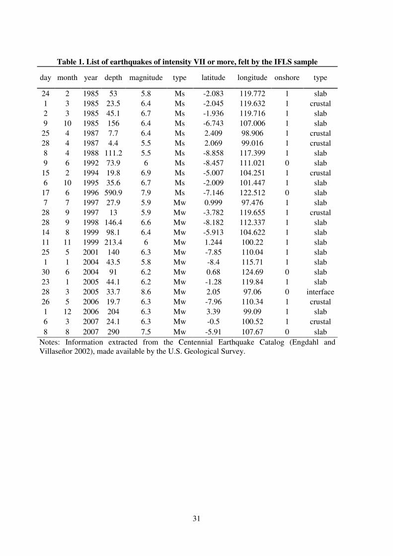
31

Table 1. List of earthquakes of intensity VII or more, felt by the IFLS sample

day month year depth magnitude type latitude longitude onshore type

24 2 1985 53 5.8 Ms -2.083 119.772 1 slab

1 3 1985 23.5 6.4 Ms -2.045 119.632 1 crustal

2 3 1985 45.1 6.7 Ms -1.936 119.716 1 slab

9 10 1985 156 6.4 Ms -6.743 107.006 1 slab

25 4 1987 7.7 6.4 Ms 2.409 98.906 1 crustal

28 4 1987 4.4 5.5 Ms 2.069 99.016 1 crustal

8 4 1988 111.2 5.5 Ms -8.858 117.399 1 slab

9 6 1992 73.9 6 Ms -8.457 111.021 0 slab

15 2 1994 19.8 6.9 Ms -5.007 104.251 1 crustal

6 10 1995 35.6 6.7 Ms -2.009 101.447 1 slab

17 6 1996 590.9 7.9 Ms -7.146 122.512 0 slab

7 7 1997 27.9 5.9 Mw 0.999 97.476 1 slab

28 9 1997 13 5.9 Mw -3.782 119.655 1 crustal

28 9 1998 146.4 6.6 Mw -8.182 112.337 1 slab

14 8 1999 98.1 6.4 Mw -5.913 104.622 1 slab

11 11 1999 213.4 6 Mw 1.244 100.22 1 slab

25 5 2001 140 6.3 Mw -7.85 110.04 1 slab

1 1 2004 43.5 5.8 Mw -8.4 115.71 1 slab

30 6 2004 91 6.2 Mw 0.68 124.69 0 slab

23 1 2005 44.1 6.2 Mw -1.28 119.84 1 slab

28 3 2005 33.7 8.6 Mw 2.05 97.06 0 interface

26 5 2006 19.7 6.3 Mw -7.96 110.34 1 crustal

1 12 2006 204 6.3 Mw 3.39 99.09 1 slab

6 3 2007 24.1 6.3 Mw -0.5 100.52 1 crustal

8 8 2007 290 7.5 Mw -5.91 107.67 0 slab

Notes: Information extracted from the Centennial Earthquake Catalog (Engdahl and

Villaseñor 2002), made available by the U.S. Geological Survey.

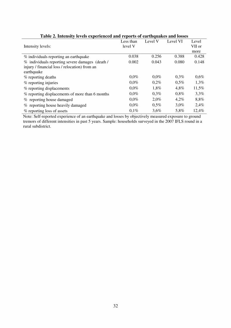
32

Table 2. Intensity levels experienced and reports of earthquakes and losses

Intensity levels:

Less than

level V

Level V Level VI Level

VII or

more

% individuals reporting an earthquake 0.038 0.256 0.388 0.428

% individuals reporting severe damages (death /

injury / financial loss / relocation) from an

earthquake

0.002 0.043 0.080 0.148

% reporting deaths 0,0% 0,0% 0,3% 0,6%

% reporting injuries 0,0% 0,2% 0,5% 1,3%

% reporting displacements 0,0% 1,8% 4,8% 11,5%

% reporting displacements of more than 6 months 0,0% 0,3% 0,8% 3,3%

% reporting house damaged 0,0% 2,0% 4,2% 8,8%

% reporting house heavily damaged 0,0% 0,5% 3,0% 2,4%

% reporting loss of assets 0,1% 3,6% 5,8% 12,4%

Note: Self-reported experience of an earthquake and losses by objectively measured exposure to ground

tremors of different intensities in past 5 years. Sample: households surveyed in the 2007 IFLS round in a

rural subdistrict.

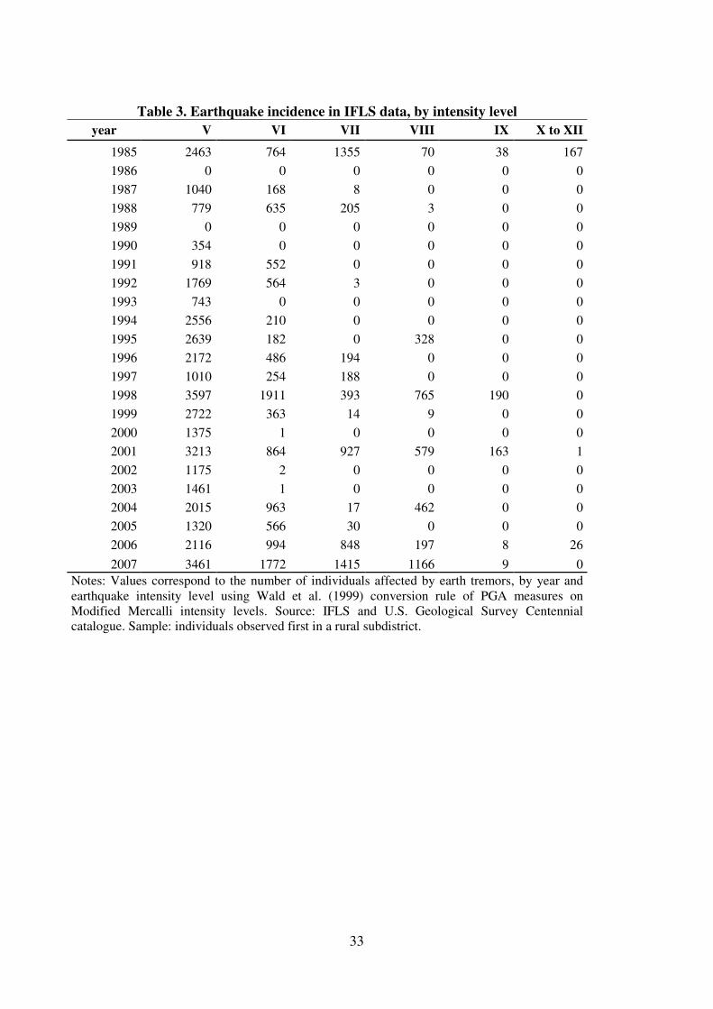
33

Table 3. Earthquake incidence in IFLS data, by intensity level

year V VI VII VIII IX X to XII

1985 2463 764 1355 70 38 167

1986 0 0 0 0 0 0

1987 1040 168 8 0 0 0

1988 779 635 205 3 0 0

1989 0 0 0 0 0 0

1990 354 0 0 0 0 0

1991 918 552 0 0 0 0

1992 1769 564 3 0 0 0

1993 743 0 0 0 0 0

1994 2556 210 0 0 0 0

1995 2639 182 0 328 0 0

1996 2172 486 194 0 0 0

1997 1010 254 188 0 0 0

1998 3597 1911 393 765 190 0

1999 2722 363 14 9 0 0

2000 1375 1 0 0 0 0

2001 3213 864 927 579 163 1

2002 1175 2 0 0 0 0

2003 1461 1 0 0 0 0

2004 2015 963 17 462 0 0

2005 1320 566 30 0 0 0

2006 2116 994 848 197 8 26

2007 3461 1772 1415 1166 9 0

Notes: Values correspond to the number of individuals affected by earth tremors, by year and

earthquake intensity level using Wald et al. (1999) conversion rule of PGA measures on

Modified Mercalli intensity levels. Source: IFLS and U.S. Geological Survey Centennial

catalogue. Sample: individuals observed first in a rural subdistrict.

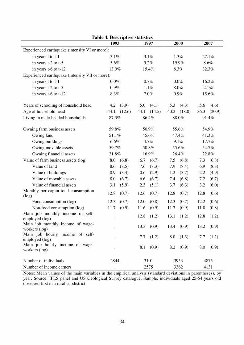
34

Table 4. Descriptive statistics

1993 1997 2000 2007

Experienced earthquake (intensity VI or more):

in years t to t-1 3.1% 3.1% 1.3% 27.1%

in years t-2 to t-5 5.6% 5.2% 19.9% 8.6%

in years t-6 to t-12 13.0% 15.4% 8.3% 32.3%

Experienced earthquake (intensity VII or more):

in years t to t-1 0.0% 0.7% 0.0% 16.2%

in years t-2 to t-5 0.9% 1.1% 8.0% 2.1%

in years t-6 to t-12 8.3% 7.0% 0.9% 15.6%

Years of schooling of household head 4.2 (3.9) 5.0 (4.1) 5.3 (4.3) 5.6 (4.6)

Age of household head 44.1 (12.6) 44.1 (14.5) 40.2 (18.0) 36.3 (20.9)

Living in male-headed households 87.3% 86.4% 88.0% 91.4%

Owning farm business assets 59.8% 50.9% 55.6% 54.9%

Owing land 51.1% 45.6% 47.4% 41.3%

Owing buildings 6.6% 4.7% 9.1% 17.7%

Owing movable assets 59.7% 50.8% 55.6% 54.7%

Owning financial assets 21.8% 16.9% 26.4% 22.8%

Value of farm business assets (log) 8.0 (6.8) 6.7 (6.7) 7.5 (6.8) 7.3 (6.8)

Value of land 8.6 (8.5) 7.6 (8.3) 7.9 (8.4) 6.9 (8.3)

Value of buildings 0.9 (3.4) 0.6 (2.9) 1.2 (3.7) 2.2 (4.9)

Value of movable assets 8.0 (6.7) 6.6 (6.7) 7.4 (6.8) 7.2 (6.7)

Value of financial assets 3.1 (5.9) 2.3 (5.1) 3.7 (6.3) 3.2 (6.0)

Monthly per capita total consumption

(log) 12.8 (0.7) 12.6 (0.7) 12.8 (0.7) 12.8 (0.6)

Food consumption (log) 12.3 (0.7) 12.0 (0.8) 12.3 (0.7) 12.2 (0.6)

Non-food consumption (log) 11.7 (0.9) 11.6 (0.9) 11.7 (0.9) 11.8 (0.8)

Main job monthly income of self-

employed (log) . 12.8 (1.2) 13.1 (1.2) 12.8 (1.2)

Main job monthly income of wage-

workers (log) . 13.3 (0.9) 13.4 (0.9) 13.2 (0.9)

Main job hourly income of self-

employed (log) . 7.7 (1.2) 8.0 (1.3) 7.7 (1.2)

Main job hourly income of wage-

workers (log) . 8.1 (0.9) 8.2 (0.9) 8.0 (0.9)

Number of individuals 2844 3101 3953 4875

Number of income earners . 2575 3362 4131

Notes: Mean values of the main variables in the empirical analysis (standard deviations in parentheses), by

year. Source: IFLS panel and US Geological Survey catalogue. Sample: individuals aged 25-54 years old

observed first in a rural subdistrict.

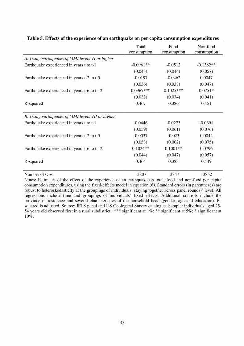
35

Table 5. Effects of the experience of an earthquake on per capita consumption expenditures

Total

consumption

Food

consumption

Non-food

consumption

A: Using earthquakes of MMI levels VI or higher

Earthquake experienced in years t to t-1 -0.0961** -0.0512 -0.1382**

(0.043) (0.044) (0.057)

Earthquake experienced in years t-2 to t-5 -0.0197 -0.0462 0.0047

(0.036) (0.038) (0.047)

Earthquake experienced in years t-6 to t-12 0.0967*** 0.1025*** 0.0751*

(0.033) (0.034) (0.041)

R-squared 0.467 0.386 0.451

B: Using earthquakes of MMI levels VII or higher

Earthquake experienced in years t to t-1 -0.0446 -0.0273 -0.0691

(0.059) (0.061) (0.076)

Earthquake experienced in years t-2 to t-5 -0.0037 -0.023 0.0044

(0.058) (0.062) (0.075)

Earthquake experienced in years t-6 to t-12 0.1024** 0.1001** 0.0796

(0.044) (0.047) (0.057)

R-squared 0.464 0.383 0.449

Number of Obs. 13807 13847 13852

Notes: Estimates of the effect of the experience of an earthquake on total, food and non-food per capita

consumption expenditures, using the fixed-effects model in equation (6). Standard errors (in parentheses) are

robust to heteroskedasticity at the groupings of individuals (staying together across panel rounds)’ level. All

regressions include time and groupings of individuals’ fixed effects. Additional controls include the

province of residence and several characteristics of the household head (gender, age and education). R-

squared is adjusted. Source: IFLS panel and US Geological Survey catalogue. Sample: individuals aged 25-

54 years old observed first in a rural subdistrict. *** significant at 1%; ** significant at 5%; * significant at

10%.

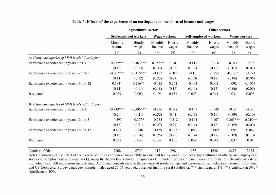
36

Table 6: Effects of the experience of an earthquake on men's rural income and wages

Agricultural sector Other sectors

Self-employed workers Wage workers Self-employed workers Wage workers

Monthly

income

Hourly

wages

Monthly

income

Hourly

wages

Monthly

income

Hourly

wages

Monthly

income

Hourly

wages

(1) (2) (3) (4) (5) (6) (7) (8)


Earthquake experienced in years t to t-1 -0.437*** -0.463*** -0.753** -0.107 -0.111 -0.118 -0.077 -0.07

(0.13) (0.13) (0.33) (0.33) (0.13) (0.16) (0.07) (0.07)

Earthquake experienced in years t-2 to t-5 -0.307*** -0.316*** -0.127 -0.07 -0.16 -0.152 -0.106* -0.073

(0.11) (0.12) (0.23) (0.24) (0.10) (0.12) (0.06) (0.06)

Earthquake experienced in years t-6 to t-12 0.181* 0.216** -0.025 0.252 -0.003 0.002 0.092 0.106*

(0.11) (0.11) (0.18) (0.17) (0.11) (0.13) (0.06) (0.06)

R-squared 0.069 0.063 0.196 0.151 0.055 0.044 0.031 0.038


Earthquake experienced in years t to t-1 -0.743*** -0.596*** -0.296 0.078 -0.151 -0.148 -0.09 -0.061

(0.20) (0.21) (0.36) (0.41) (0.15) (0.19) (0.09) (0.10)

Earthquake experienced in years t-2 to t-5 -0.293 -0.373* -0.255 -0.212 -0.144 -0.107 -0.263*** -0.210**

(0.18) (0.21) (0.27) (0.29) (0.14) (0.16) (0.09) (0.09)

Earthquake experienced in years t-6 to t-12 0.191 0.246 -0.159 0.033 0.051 -0.069 0.092 0.087

(0.15) (0.16) (0.25) (0.29) (0.14) (0.17) (0.09) (0.10)

R-squared 0.062 0.051 0.139 0.135 0.049 0.042 0.037 0.04

Number of Obs. 2808 2790 912 898 1657 1628 2676 2625

Notes: Estimates of the effect of the experience of an earthquake on monthly income and hourly wages, by sector (agricultural and others) and employment

status (self-employment and wage work), using the fixed-effects model in equation (1). Standard errors (in parentheses) are robust to heteroskedasticity at

individual level. All regressions include time. Additional controls include the province of residence, age and age-squared, and education. Source: IFLS panel

and US Geological Survey catalogue. Sample: males aged 25-54 years old observed first in a rural subdistrict. *** significant at 1%; ** significant at 5%; *

significant at 10%.

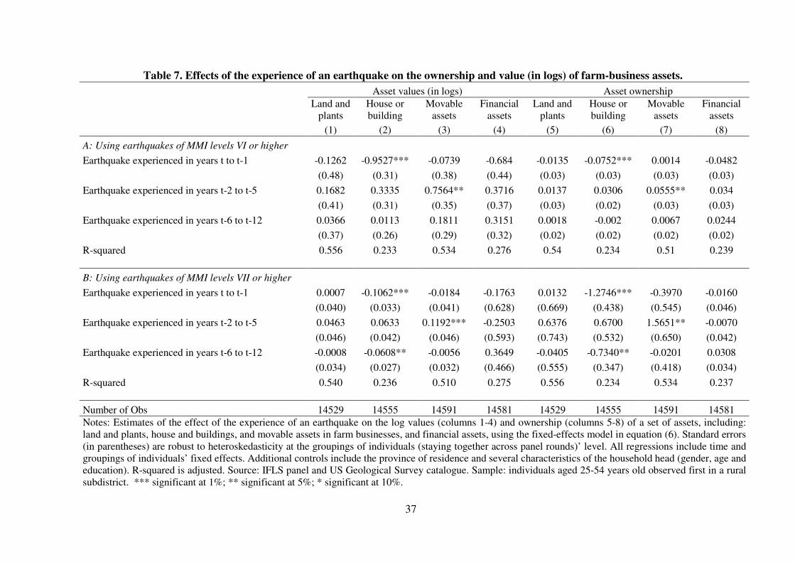
37

Table 7. Effects of the experience of an earthquake on the ownership and value (in logs) of farm-business assets.

Asset values (in logs) Asset ownership

Land and

plants

House or

building

Movable

assets

Financial

assets

Land and

plants

House or

building

Movable

assets

Financial

assets

(1) (2) (3) (4) (5) (6) (7) (8)


Earthquake experienced in years t to t-1 -0.1262 -0.9527*** -0.0739 -0.684 -0.0135 -0.0752*** 0.0014 -0.0482

(0.48) (0.31) (0.38) (0.44) (0.03) (0.03) (0.03) (0.03)

Earthquake experienced in years t-2 to t-5 0.1682 0.3335 0.7564** 0.3716 0.0137 0.0306 0.0555** 0.034

(0.41) (0.31) (0.35) (0.37) (0.03) (0.02) (0.03) (0.03)

Earthquake experienced in years t-6 to t-12 0.0366 0.0113 0.1811 0.3151 0.0018 -0.002 0.0067 0.0244

(0.37) (0.26) (0.29) (0.32) (0.02) (0.02) (0.02) (0.02)

R-squared 0.556 0.233 0.534 0.276 0.54 0.234 0.51 0.239


Earthquake experienced in years t to t-1 0.0007 -0.1062*** -0.0184 -0.1763 0.0132 -1.2746*** -0.3970 -0.0160

(0.040) (0.033) (0.041) (0.628) (0.669) (0.438) (0.545) (0.046)

Earthquake experienced in years t-2 to t-5 0.0463 0.0633 0.1192*** -0.2503 0.6376 0.6700 1.5651** -0.0070

(0.046) (0.042) (0.046) (0.593) (0.743) (0.532) (0.650) (0.042)

Earthquake experienced in years t-6 to t-12 -0.0008 -0.0608** -0.0056 0.3649 -0.0405 -0.7340** -0.0201 0.0308

(0.034) (0.027) (0.032) (0.466) (0.555) (0.347) (0.418) (0.034)

R-squared 0.540 0.236 0.510 0.275 0.556 0.234 0.534 0.237

Number of Obs 14529 14555 14591 14581 14529 14555 14591 14581

Notes: Estimates of the effect of the experience of an earthquake on the log values (columns 1-4) and ownership (columns 5-8) of a set of assets, including:

land and plants, house and buildings, and movable assets in farm businesses, and financial assets, using the fixed-effects model in equation (6). Standard errors

(in parentheses) are robust to heteroskedasticity at the groupings of individuals (staying together across panel rounds)’ level. All regressions include time and

groupings of individuals’ fixed effects. Additional controls include the province of residence and several characteristics of the household head (gender, age and

education). R-squared is adjusted. Source: IFLS panel and US Geological Survey catalogue. Sample: individuals aged 25-54 years old observed first in a rural

subdistrict. *** significant at 1%; ** significant at 5%; * significant at 10%.

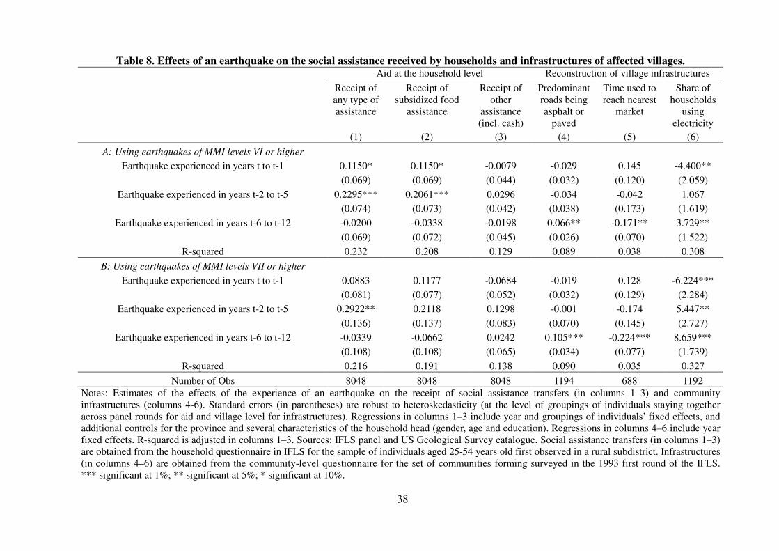
38

Table 8. Effects of an earthquake on the social assistance received by households and infrastructures of affected villages. Aid at the household level Reconstruction of village infrastructures

Receipt of

any type of

assistance

Receipt of

subsidized food

assistance

Receipt of

other

assistance

(incl. cash)

Predominant

roads being

asphalt or

paved

Time used to

reach nearest

market

Share of

households

using

electricity

(1) (2) (3) (4) (5) (6)


Earthquake experienced in years t to t-1 0.1150* 0.1150* -0.0079 -0.029 0.145 -4.400**

(0.069) (0.069) (0.044) (0.032) (0.120) (2.059)

Earthquake experienced in years t-2 to t-5 0.2295*** 0.2061*** 0.0296 -0.034 -0.042 1.067

(0.074) (0.073) (0.042) (0.038) (0.173) (1.619)

Earthquake experienced in years t-6 to t-12 -0.0200 -0.0338 -0.0198 0.066** -0.171** 3.729**

(0.069) (0.072) (0.045) (0.026) (0.070) (1.522)

R-squared 0.232 0.208 0.129 0.089 0.038 0.308


Earthquake experienced in years t to t-1 0.0883 0.1177 -0.0684 -0.019 0.128 -6.224***

(0.081) (0.077) (0.052) (0.032) (0.129) (2.284)

Earthquake experienced in years t-2 to t-5 0.2922** 0.2118 0.1298 -0.001 -0.174 5.447**

(0.136) (0.137) (0.083) (0.070) (0.145) (2.727)

Earthquake experienced in years t-6 to t-12 -0.0339 -0.0662 0.0242 0.105*** -0.224*** 8.659***

(0.108) (0.108) (0.065) (0.034) (0.077) (1.739)

R-squared 0.216 0.191 0.138 0.090 0.035 0.327

Number of Obs 8048 8048 8048 1194 688 1192

Notes: Estimates of the effects of the experience of an earthquake on the receipt of social assistance transfers (in columns 1–3) and community

infrastructures (columns 4-6). Standard errors (in parentheses) are robust to heteroskedasticity (at the level of groupings of individuals staying together

across panel rounds for aid and village level for infrastructures). Regressions in columns 1–3 include year and groupings of individuals’ fixed effects, and

additional controls for the province and several characteristics of the household head (gender, age and education). Regressions in columns 4–6 include year

fixed effects. R-squared is adjusted in columns 1–3. Sources: IFLS panel and US Geological Survey catalogue. Social assistance transfers (in columns 1–3)

are obtained from the household questionnaire in IFLS for the sample of individuals aged 25-54 years old first observed in a rural subdistrict. Infrastructures

(in columns 4–6) are obtained from the community-level questionnaire for the set of communities forming surveyed in the 1993 first round of the IFLS.

*** significant at 1%; ** significant at 5%; * significant at 10%.

39

APPENDIX

A.1. Zhao et al. (2006) Attenuation relation for estimating local intensities of ground motions

The Zhao et al. attenuation relation, predicting the local record j for seismic event i, is the following

(equation (1) p.901 in Zhao et al., 2006):

( ) ( ) ( ) iijkijeSLSLRhcijeijwiij v+u+C+xS+S+S+F+δhhe+rbx+aM=PGA loglog log −−

with ( )wiijij dMcexp+x=r and where PGA is expressed in terms of g (the constant measuring the

acceleration due to gravity, with value of 980 cm/second squared)); wiM is moment magnitude

(measured in dyn.cm10

); ji,x is the source distance

11 (in kilometers); h is the focal depth (in

kilometers, capped at 125 km); ch is a depth constant (taking the value of 15 km);

hδ is a dummy

variable that equals 0 for ch<h and 1 for chh ≥ (implying that the depth term only takes effect

for depths larger than a certain level; RF is a reverse fault parameter that applies to some crustal

events, LS parameter applies to interface events, and SS and

SLS to subduction slab events.12

kC ,

for k=1,...,4, is a parameter for the type of local soils distinguishing rocks, hard soil, medium soil,

and soft soil13

; the error term of this random effects model contains an event specific effect iv and

an intra-event recording error ji,u . The estimated values of the Zhao et al. model parameters are:

1.101=a , 0.00564−=b , 0.0055=c , 1.080=d , 0.01412=e , RS , 0=S L , 2.607=SS,

0.528−=SSL, 0.293=CH , 1.3553 =C .

10 A dyn is a unit of force and 1 dyn = 1 g·cm/s².

11 Source distance is either the shortest distance to the rupture zone or hypocentral distance. We use the latter

as we don't have fault models for the earthquakes under study and using those would be computationally

intractable. The hypocenter of an earthquake is the position where the source fault began to rupture. It is

located at the focal depth below the epicenter. 12 All the earthquakes in our dataset are classified by type using information on focal depth and whether their

epicenter is located on- or off-shore: crustal earthquakes are events onshore with depth lower than 25

kilometers, interface events are offshore and with depth lower than 50 kilometers, and slab events have depth

larger than 50 kilometers offshore or 25 kilometers onshore (one would ideally consider the fault mechanism

with interface events having a reverse mechanism and slab events a normal one). We thank Stephan Harmsen

for his help in identifying earthquake types. 13

The type of soil matters for determining local damages, as in particular soft soils tend to amplify those.

Specific geographic environments such as ridges and hills also enter in the process. However, since we don't

have detailed information on local environments nor on soils for Indonesia, we assume medium soils

( k= 3 ) for our predictions.

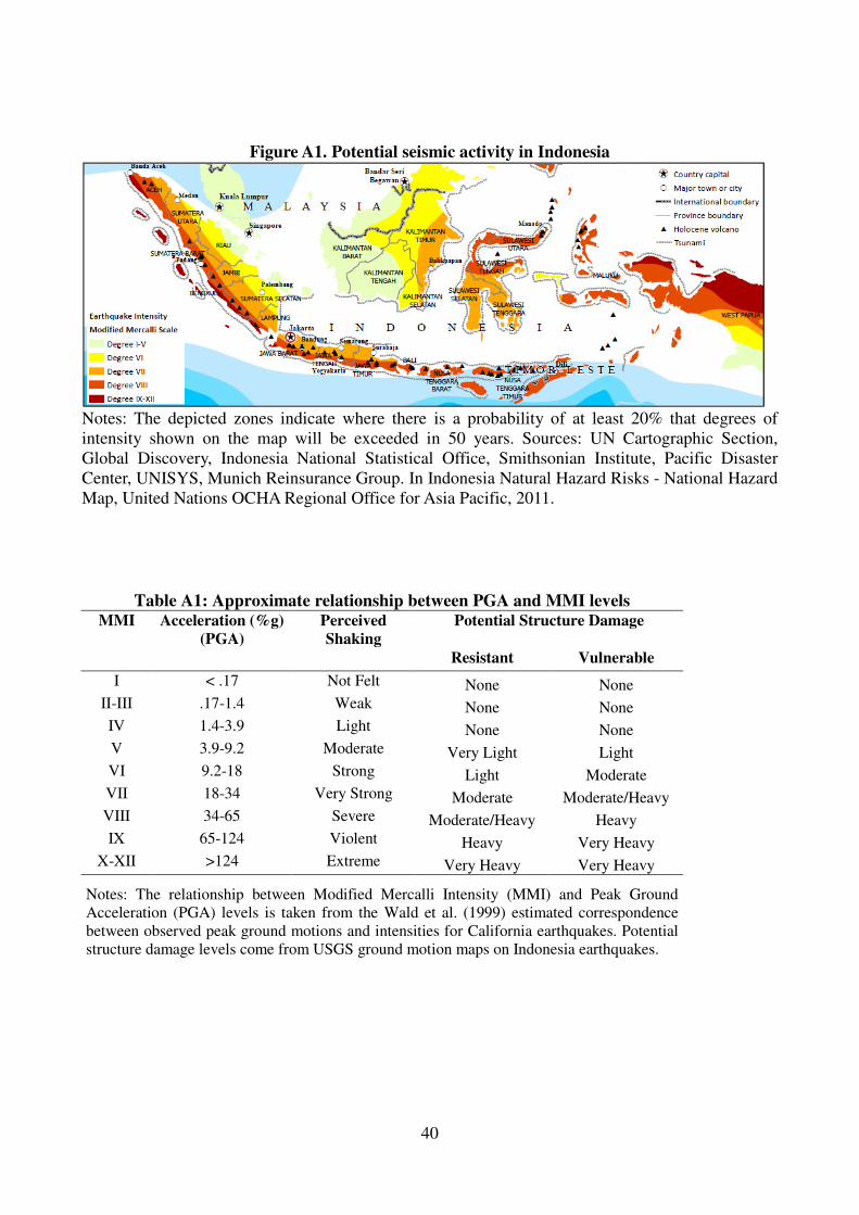
40

Figure A1. Potential seismic activity in Indonesia

Notes: The depicted zones indicate where there is a probability of at least 20% that degrees of

intensity shown on the map will be exceeded in 50 years. Sources: UN Cartographic Section,

Global Discovery, Indonesia National Statistical Office, Smithsonian Institute, Pacific Disaster

Center, UNISYS, Munich Reinsurance Group. In Indonesia Natural Hazard Risks - National Hazard

Map, United Nations OCHA Regional Office for Asia Pacific, 2011.

Table A1: Approximate relationship between PGA and MMI levels MMI Acceleration (%g)

(PGA)

Perceived

Shaking

Potential Structure Damage

Resistant Vulnerable

I < .17 Not Felt None None

II-III .17-1.4 Weak None None

IV 1.4-3.9 Light None None

V 3.9-9.2 Moderate Very Light Light

VI 9.2-18 Strong Light Moderate

VII 18-34 Very Strong Moderate Moderate/Heavy

VIII 34-65 Severe Moderate/Heavy Heavy

IX 65-124 Violent Heavy Very Heavy

X-XII >124 Extreme Very Heavy Very Heavy

Notes: The relationship between Modified Mercalli Intensity (MMI) and Peak Ground

Acceleration (PGA) levels is taken from the Wald et al. (1999) estimated correspondence

between observed peak ground motions and intensities for California earthquakes. Potential

structure damage levels come from USGS ground motion maps on Indonesia earthquakes.

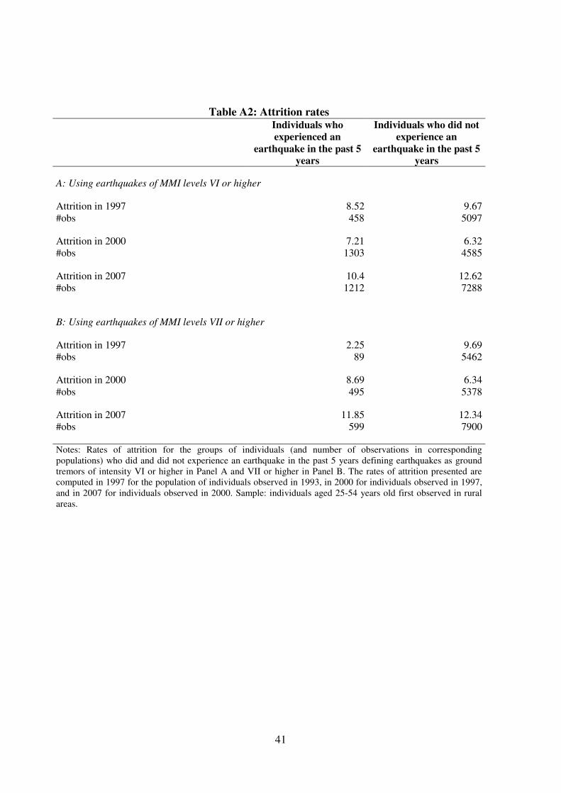
41

Table A2: Attrition rates

Individuals who

experienced an

earthquake in the past 5

years

Individuals who did not

experience an

earthquake in the past 5

years


Attrition in 1997 8.52 9.67

#obs 458 5097


#obs 1303 4585

Attrition in 2007 10.4 12.62

#obs 1212 7288



#obs 89 5462


#obs 495 5378

Attrition in 2007 11.85 12.34

#obs 599 7900 Notes: Rates of attrition for the groups of individuals (and number of observations in corresponding

populations) who did and did not experience an earthquake in the past 5 years defining earthquakes as ground

tremors of intensity VI or higher in Panel A and VII or higher in Panel B. The rates of attrition presented are

computed in 1997 for the population of individuals observed in 1993, in 2000 for individuals observed in 1997,

and in 2007 for individuals observed in 2000. Sample: individuals aged 25-54 years old first observed in rural

areas.

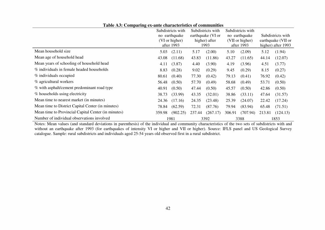
42

Table A3: Comparing ex-ante characteristics of communities

Subdistricts with

no earthquake

(VI or higher)

after 1993

Subdistricts with

earthquake (VI or

higher) after

1993

Subdistricts with

no earthquake

(VII or higher)

after 1993

Subdistricts with

earthquake (VII or

higher) after 1993

Mean household size 5.03 (2.11) 5.17 (2.00) 5.10 (2.09) 5.12 (1.94)

Mean age of household head 43.08 (11.68) 43.83 (11.86) 43.27 (11.65) 44.14 (12.07)

Mean years of schooling of household head 4.11 (3.87) 4.40 (3.90) 4.19 (3.96) 4.51 (3.77)

% individuals in female headed households 8.83 (0.28) 9.02 (0.29) 9.45 (0.29) 8.15 (0.27)

% individuals occupied 80.61 (0.40) 77.30 (0.42) 79.13 (0.41) 76.92 (0.42)

% agricultural workers 56.48 (0.50) 57.70 (0.49) 58.68 (0.49) 53.71 (0.50)

% with asphalt/cement predominant road type 40.91 (0.50) 47.44 (0.50) 45.57 (0.50) 42.86 (0.50)

% households using electricity 38.73 (33.99) 43.35 (32.01) 38.86 (33.11) 47.64 (31.57)

Mean time to nearest market (in minutes) 24.36 (17.16) 24.35 (23.48) 25.39 (24.07) 22.42 (17.24)

Mean time to District Capital Center (in minutes) 78.84 (62.59) 72.31 (87.76) 79.94 (83.94) 65.48 (71.51)

Mean time to Provincial Capital Center (in minutes) 359.98 (902.25) 237.44 (267.17) 306.91 (707.94) 213.81 (124.13)

Number of individual observations involved 1981 3392 3388 1853

Notes: Mean values (and standard deviations in parenthesis) of the individual and community characteristics of the two sets of subdistricts with and

without an earthquake after 1993 (for earthquakes of intensity VI or higher and VII or higher). Source: IFLS panel and US Geological Survey

catalogue. Sample: rural subdistricts and individuals aged 25-54 years old observed first in a rural subdistrict.

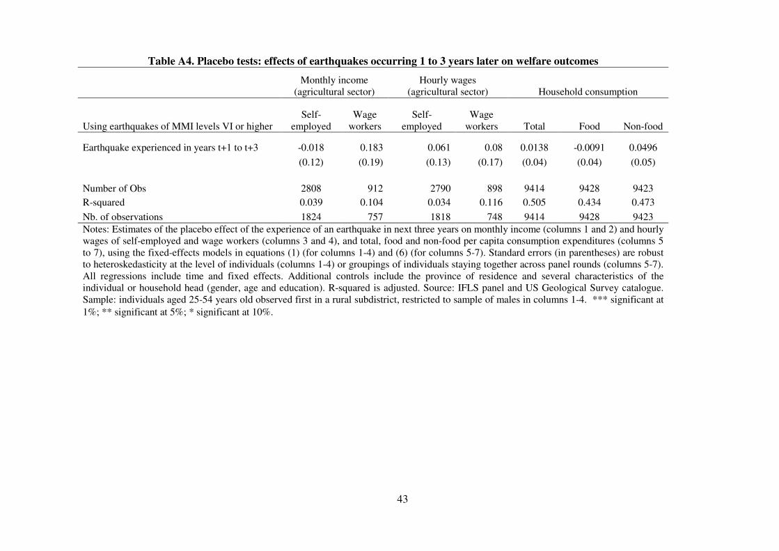
43

Table A4. Placebo tests: effects of earthquakes occurring 1 to 3 years later on welfare outcomes

Monthly income

(agricultural sector)

Hourly wages

(agricultural sector) Household consumption

Using earthquakes of MMI levels VI or higher

Self-

employed

Wage

workers

Self-

employed

Wage

workers Total Food Non-food

Earthquake experienced in years t+1 to t+3 -0.018 0.183 0.061 0.08 0.0138 -0.0091 0.0496

(0.12) (0.19) (0.13) (0.17) (0.04) (0.04) (0.05)

Number of Obs 2808 912 2790 898 9414 9428 9423

R-squared 0.039 0.104 0.034 0.116 0.505 0.434 0.473

Nb. of observations 1824 757 1818 748 9414 9428 9423

Notes: Estimates of the placebo effect of the experience of an earthquake in next three years on monthly income (columns 1 and 2) and hourly

wages of self-employed and wage workers (columns 3 and 4), and total, food and non-food per capita consumption expenditures (columns 5

to 7), using the fixed-effects models in equations (1) (for columns 1-4) and (6) (for columns 5-7). Standard errors (in parentheses) are robust

to heteroskedasticity at the level of individuals (columns 1-4) or groupings of individuals staying together across panel rounds (columns 5-7).

All regressions include time and fixed effects. Additional controls include the province of residence and several characteristics of the

individual or household head (gender, age and education). R-squared is adjusted. Source: IFLS panel and US Geological Survey catalogue.

Sample: individuals aged 25-54 years old observed first in a rural subdistrict, restricted to sample of males in columns 1-4. *** significant at

1%; ** significant at 5%; * significant at 10%.

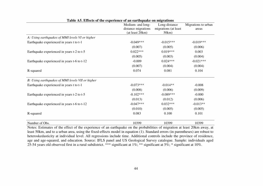
44

Table A5. Effects of the experience of an earthquake on migrations Medium- and long-

distance migrations

(at least 20km)

Long-distance

migrations (at least

50km)

Migrations to urban

areas


Earthquake experienced in years t to t-1 -0.049*** -0.015*** -0.019***

(0.007) (0.005) (0.006)

Earthquake experienced in years t-2 to t-5 0.022*** 0.019*** 0.003

(0.005) (0.003) (0.004)

Earthquake experienced in years t-6 to t-12 -0.009 0.024*** -0.021***

(0.007) (0.004) (0.004)

R-squared 0.074 0.081 0.104


Earthquake experienced in years t to t-1 -0.073*** -0.014** -0.008

(0.008) (0.006) (0.009)

Earthquake experienced in years t-2 to t-5 -0.102*** -0.089*** -0.000

(0.013) (0.012) (0.006)

Earthquake experienced in years t-6 to t-12 -0.047*** 0.032*** -0.013**

(0.010) (0.005) (0.005)

R-squared 0.083 0.100 0.101

Number of Obs. 10399 10399 10399

Notes: Estimates of the effect of the experience of an earthquake on the probabilities of migration at least 20km away, at

least 50km, and to a urban area, using the fixed-effects model in equation (1). Standard errors (in parentheses) are robust to

heteroskedasticity at individual level. All regressions include time. Additional controls include the province of residence,

age and age-squared, and education. Source: IFLS panel and US Geological Survey catalogue. Sample: individuals aged

25-54 years old observed first in a rural subdistrict. *** significant at 1%; ** significant at 5%; * significant at 10%.

Long-run effects of earthquakes on welfare in rural Indonesia

Documents

Transcript of Long-run effects of earthquakes on welfare in rural Indonesia