Intertemporal Welfare Dynamics

Background Paper for HDR 2001

Shahin Yaqub1 Sussex University

England

October 2000

1 The author is a doctoral candidate researching ‘Born Poor, Stay Poor? The Intergenerational Persistence of Poverty.’ Contact details: Poverty Research Unit AFRAS, Sussex University, Falmer Brighton BN1 9QN. Email: s.yaqub@sussex.ac.uk. Thanks to Sunniyat Rahman, Reetika Khera and Silvia Jarauta Bernal for their help.

Shahin Yaqub

ii

Contents

1 INTRODUCTION ..................................................................................................................................1

1.1 CONCEPTUAL ISSUES ..........................................................................................................................1 1.1.1 Insecurity and opportunity within economic mobility ...............................................................1 1.1.2 Mobility and human development: complementary concepts? .................................................3 1.1.3 Relative and absolute, in mobility and poverty..........................................................................4

1.2 MEASUREMENT ISSUES.......................................................................................................................4 1.2.1 Types of data...............................................................................................................................4 1.2.2 Types of models: components versus spells ...............................................................................5 1.2.3 Illusionary and spurious dynamics ............................................................................................6

2 EXTENT OF WELFARE DYNAMICS...............................................................................................8

2.1 ECONOMIC MOBILITY .........................................................................................................................8 2.2 CHRONIC POVERTY ...........................................................................................................................10 2.3 LINKING MOBILITY TO CHRONIC POVERTY.......................................................................................12 2.4 LINKING MOBILITY TO TRANSITORY POVERTY.................................................................................19 2.5 LINKING MOBILITY TO INEQUALITY, GROWTH, AND POVERTY.........................................................21

3 EXPLAINING WELFARE DYNAMICS..........................................................................................21

3.1 SOCIO-ECONOMIC CORRELATES OF MOBILITY..................................................................................21 3.1.1 Discussion of methods ..............................................................................................................21 3.1.2 Summary of results ...................................................................................................................22

3.2 THE ‘SILVER SPOON, PLASTIC SPOON’ HYPOTHESIS..........................................................................25 3.2.1 Intergenerational and sibling correlations: reduced form explanations ................................25

Intergenerational correlations.........................................................................................................................26 Sibling and twin correlations..........................................................................................................................29

3.2.2 What do parental and sibling variables represent?.................................................................30 Role of money ................................................................................................................................................30 Education ........................................................................................................................................................34 Culture, class and community ........................................................................................................................36

3.3 SAME FAMILY BUT DIFFERENT: INTRAHOUSEHOLD BIASES..............................................................38

4 CONCLUSION .....................................................................................................................................41

REFERENCES – INTERTEMPORAL WELFARE DYNAMICS ...................................................44

Shahin Yaqub

iii

Tables, figures and annexes

Table 1: Estimates of economic mobility, excluding taxes and transfers ..................................................9

Table 2: Estimates of economic mobility, including taxes and transfers .................................................10

Table 3: Absolute poverty persistence ......................................................................................................11

Table 4: Relative poverty persistence .......................................................................................................12

Table 5: Immobility: % of population in same quintile in base year and final year ................................14

Table 6: Share of mobility to adjacent quintile in total mobility..............................................................15

Table 7: Transitory fluctuations by ventile of permanent income............................................................16

Table 8: Inequality in permanent income..................................................................................................18

Table 9: State dependency: % of poor remaining poor after T years of poverty .....................................19

Table 10: Percent of population by years of poverty in the period covered by the panel........................20

Table 11: Summary of studies identifying mobility correlates.................................................................23

Table 12: Poverty experiences by age 16 in USA, according to parental characteristics ........................25

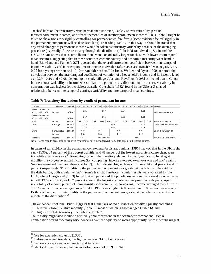
Table 13: Intergenerational income correlations.......................................................................................27

Table 14: Intergenerational earnings correlations.....................................................................................27

Table 15: Intergenerational income-needs and wage rate correlations ....................................................28

Table 16: Intergenerational poverty transition matrix, UK (% of offspring) ...........................................28

Table 17 Sibling Correlations in Status Hungary .....................................................................................30

Table 18: Intergenerational Transmission of Education in Africa ...........................................................35

Table 19 Effect of Extra Education on Probability of Upward Mobility from Unskilled Work .............36

Figure 1: Linking mobility to chronic poverty..........................................................................................13

Figure 2: Distribution of total years of poverty in four panels, shown with Lorenz curves ....................20

Figure 3 Classification of variables explaining dynamics ........................................................................22

Annex Table 1: Percentage population in same wealth quintile in 1966 and 1981, USA .......................42

Annex Table 2: Life-cycle changes in mobility........................................................................................42

Annex Table 3: Impact of methodology on intergenerational mobility estimates: theory ......................42

Annex Table 4: Impact of methodology on intergenerational mobility estimates: applied.....................43

Shahin Yaqub

1

1 Introduction This paper examines welfare through time. Too often trends in aggregate welfare statistics – such as growth in mean welfare in a population, and changes in inequality in welfare levels – have been taken to equal changes in individual welfare over time. This would characterise, for example, most welfare analyses of macroeconomic structural adjustment and stabilisation in developing countries during the heated debates of the 1980s. Also persistently high inequality or poverty have been taken to demonstrate low mobility, and unequal socio-economic opportunities. In other research, welfare variations across people have been used to address questions which are really about welfare variations through time – the worst of these are ‘poverty probits’ which crudely correlate socio-economic characteristics to poverty status observed in a cross-section.2 Such studies treat people as having no personal history – the welfare status of a person is ahistorical, seen in a snapshot moment. Key policy debates, such as the links between poverty, growth and inequality, frequently have ignored mobility even though quite different social choices may be present: is it better to have a minority permanently in poverty (low poverty, low mobility), or a majority frequently in and out of poverty (high poverty, high mobility)? Do clear policy instruments even exist to present such a choice in the first place? And where rising inequality “penalises” economic growth in its welfare impact, does rising mobility “forgive” rising inequality? If so, the quality of economic growth should not only consider distribution neutrality [UNDP 1996], but also mobility neutrality. The welfare costs of vulnerability, risk and insecurity often have been left out, as have the welfare benefits of socio-economic opportunity. Both over the life-course, and over much shorter timeframes, welfare is subject to intertemporal variations in ways which are not captured by trends in mean welfare in the population or changes in inequality, and which are difficult to assess within cross-sectional samples of people. This paper synthesises the evidence on intertemporal welfare dynamics in developing and industrial countries. The paper relates economic dynamics to two welfare issues: insecurity and opportunity (section 1.1.1), and human development, as defined by UNDP (section 1.1.2). The paper also brings microeconomic evidence on mobility to bear on chronic and transitory poverty (sections 2.3 and 2.4). International comparisons on these issues are cautioned by some important measurement issues related to choices over data, models, and methodology (section 1.2). Turning to explanations of intertemporal welfare dynamics the paper first assembles evidence on the socio-economic correlates of welfare dynamics (section 3.1). These identify the socio-economic characteristics which are correlated with different kinds of mobility. Explanations of welfare dynamics are mainly of this form, although methodologically they actually explain little, and most studies relate to short-run mobility. The paper then focuses on the determinants of long-run mobility. One event thought to be influential in determining lifetime mobility is being born poor. Intergenerational studies correlate parental and offspring welfare, and sibling studies examine welfare divergences between siblings (section 3.2.1). This paper interprets these two types of studies as ways of measuring the impact of childhood background on subsequent lifetime mobility. Several types of results exist from quite different areas of research which identify specific channels by which life-time mobility may be determined by pre-adult experiences (section 3.2.2). Finally as elsewhere, the assumption of the unitary household is imperfect. So a closing section presents intrahousehold issues in determining long-run dynamics (section 3.3).

1.1 Conceptual issues

1.1.1 Insecurity and opportunity within economic mobility Transitory and permanent component of welfare. Lots of random and non-random events happen in a person’s life. These determine welfare dynamics. But the welfare effects of some events last longer than others. This difference gives rise to short-run and long-run welfare dynamism. The usual approach is to

2 A poverty probit regresses a set of socio-economic variables on a dependent variable which is either zero (if the person is nonpoor) or one (if the person is poor). See Pudney [1999] for fuller discussion of problems with poverty probits and logits.

Shahin Yaqub

2

conceptualise the welfare of a person as having short-run variations around some typical or ‘permanent’ welfare level. For example, from time to time income may differ from a person’s typical income level due to macroeconomic conditions, bouts of illness, or weather. By definition, the average over time of each person’s transitory deviations from their permanent level equals zero in this simple model. Not only the frequency, but also the amplitude, of these transitory divergences from permanent welfare levels might differ across people, space and periods. Thus income measured at any single point in time can be stated as being partly ‘permanent’ and partly transitory. Consequently also inequality at any single point in time has two components: inequality in ‘permanent’ welfare levels, plus inequality in transitory welfare due to people being temporarily in different parts of the inequality distribution from their typical position. Similarly poverty – defined as a shortfall below some minimum welfare standard – can therefore also have a permanent component and a transitory component. Shortfalls in the permanent component are commonly used to define chronic poverty. Conceptually this approach could be applied to any welfare indicator, with the expectation that the relative sizes of the permanent component and transitory component will differ from measure to measure because welfare indicators differ in their variability over time. Trends in the permanent component. Much of the literature focuses on the transitory component as the source of welfare dynamism. Commonly the permanent component is defined as the intertemporal average of the welfare indicator, such as a person’s income averaged over several years. This approach therefore assumes that over the reference period the permanent component is just that: permanent. The transitory component at any particular point in time is defined as the difference between the level of the welfare indicator at that time, and the permanent component. If indeed the transitory component does not sum to zero over time, it would mean the level of the ‘permanent’ component had changed. Clearly this approach is best suited to dynamics over the short-run where it may be assumed that the permanent component is not changing perceptibly, and barring events which alter people’s permanent welfare levels. Over longer periods the permanent level may itself be evolving due to life-cycle effects, long-run macroeconomic growth, or labour market shifts due to changes in the skills composition of production. Permanent welfare also may take a sudden change due to an irreversible alteration in circumstance, such as through accidental physical disability, or the changes which occurred when countries abandoned central economic planning. In this sense the so-called ‘permanent’ component may be better regarded as a trend component with potential structural breaks associated with particular ‘life-altering’ events. Applied over the longer-run, the averaging procedure for determining the permanent component would lead to some effects being erroneously attributed to transitory dynamism, when in fact they would be better regarded as dynamism in the permanent component. Confirming this, Björklund and Palme [1997, p.20] show that in Sweden transitory income dynamics around the intertemporal mean are substantially greater than around the time trend.3 Gottschalk [1982] used USA data, and found that for the sample as a whole about 30 percent of the intertemporal variance in earnings was due to trend effects, rather than transitory effects.4 Ramos [1999, Table 2] used UK data and found little trend effects in earnings over five years. If its determinants could be known, modelling the permanent component directly would seem to be better. Especially important would be the difference between life-cycle versus ‘other effects’ on the trend component: some changes may be due to “the life cycle of family needs, and we may regard these

3 Using a Swedish panel, Björklund and Palme [1997, pp.18-20] estimated separate quadratic trends for the income paths of each person over a period of 18 years:

yt = α + β1 t + β2 t2 + εt , where y is income, t is time and ε is i.i.d error The R2 differs across people, and by different income concepts. For individual incomes the average R2 in a group aged 18-32 years in 1974 was 0.52, compared to an average R2 of 0.25 for an older group aged 33-47 in 1974. The average R2 for disposable equivalised family income were 0.49 and 0.40, respectively. The results confirm that a stronger time trend exists at earlier ages. The transitory component (measured as a version of the Theil index) for personal income is on average 0.29 around intertemporal mean and 0.19 around trend path in the younger group. For the older group these are 0.49 and 0.41 respectively, still indicating an effect from a time trend in the permanent component. 4 Gottschalk [1982, Table 2] found that whilst 2.1 percent of the population were always under the low earnings threshold between 1966 and 1975, if earnings predicted from a trend equation was used (i.e. the transitory component was removed), the proportion increased to 4.6 percent.

Shahin Yaqub

3

differently from a situation where there has been an improvement in, say, the earning power of the family head” [Atkinson, 1996, p.71]. Distinguishing insecurity from opportunity. This distinction between the transitory and trend components of dynamics seems especially important for policy purposes, because it helps explain why to some “mobility is a double-edged sword” [OECD 1997, p.50]. Seeing mobility as just ‘one sword with two edges’ is to obfuscate two conceptually distinct components underlying the dynamics, and thereby potentially confuse the pros and cons of different kinds of policy reforms. Sometimes mobility represents insecurity, and other times opportunity. Insecurity is unwanted mobility, and opportunity is wanted mobility. In the literature, the use of the word mobility for both is confusing, and they are often not separated in analysis. For the majority transitory variations reduce welfare.5 People generally attempt to intertemporally smooth welfare, through formal and informal insurance and finance, and through risk averse behaviour. Some aversion responses may even trap people at stable but low levels of welfare (e.g. Lipton’s ‘survival algorithm’). But people also take risks to elevate their chances for long-run welfare mobility (e.g. the account in Birdsall et al. [1999] of contrasting long-run household behaviour in Brazil and South Korea). “Risk is not just a negative phenomenon – something to be avoided or minimized. It is at the same time the energizing principle of a society that has broken away from tradition and nature… Opportunity and innovation are the positive sides of risk. No one can escape risk, of course, but there is a basic difference between the passive experience of risk and the active exploration… Risk isn’t exactly the same as danger” [Giddens 1998, pp.63-4]. Wider debates. Insecurity and opportunity seems to be a central tension implicit in several policy debates. Redistribution, poverty reduction, and growth have options which differently affect a person’s permanent and transitory components of welfare. Give a person fish (income) and you may affect their transitory welfare, give them a fishing net (asset) and you may alter the trend in their permanent welfare. The discussion on linking relief interventions and development interventions could be recast in terms of policies addressing transitory and trend welfare components: “the ideal model is one in which relief and development interventions are implemented harmoniously to provide poor people with secure livelihoods and efficient safety-nets, mitigating the frequency and impact of shocks and easing rehabilitation” [Buchanan-Smith and Maxwell 1994, p.3]. Recent evidence on how income inequality hinders income growth makes little use of the permanent and transitory distinction implicit in inequality at any single point in time, although one would suspect that the mechanisms linking growth to inequality would differ between inequality in the permanent component and that in the transitory component. Findings by Deininger and Olinto [2000] that land inequality hinders growth, strongly support this. Herring [1998] makes a similar argument by contrasting the land reform experiences in Kerela, India with that of the USA in the late 19th century. The distinction also is implicit in other massive debates: globalisation (of markets, trade and information) might increase insecurity as well as opportunity in the sense that welfare may become more exposed to transitory shocks at the same time as showing a stronger trend growth; fiscal belt-tightening is inescapable for macroeconomic stabilisation in some countries, but the case of its detractors lies ultimately in whether such belt-tightening is so savage as to impair the permanent component of welfare (i.e. stabilised chronic poverty); after socialism, households faced both insecurity and opportunity as socialist organisation was dismantled and markets were introduced. These discussions are too large to include further in this paper.

1.1.2 Mobility and human development: complementary concepts? There are two sides to UNDP’s conception of human development: “One is the formation of human capabilities, such as improved health or knowledge. The other is the use that people make of their acquired capabilities” [UNDP 1990, p.10]. Notably the presentation, measurement, and application by UNDP of the human development concept is not dynamic, having had a greater practical focus on the levels and trends in capabilities (c.f. for example the different development indices used by UNDP). Yet both sides of human development are central explanatory motivations in the welfare dynamics research. According to their capabilities, people differ not only in the extent of transitory dynamics in their welfare, but also in the trend path of the permanent component of welfare over their lifetime. Some people’s trend path never rises above

5 See Bird [1995] for discussion of welfare costs of transitory income.

Shahin Yaqub

4

the poverty line, and they forever remain poor. The data for these statements are shown in section 2.1, and section 3.1 suggests that the variations across people in mobility may be according to their human capabilities. It might be argued that antipoverty policy finds it harder to trigger a sustained rise in a poor person’s trend component of welfare, than to ameliorate the poverty due to transitory fluctuations (especially where chronic poverty exists). In particular, the presentation in section 3.2 of intergenerational and sibling research raises issues over the role of childhood experiences in the formation of capabilities which people may carry through life. These capabilities may set a person on a particular intertemporal welfare path. Moreover the second aspect of human development, the freedom to utilise capabilities, strongly determines welfare dynamics. Economic insecurity and opportunity, discussed above as different dimensions of mobility, are central to ‘how, which and whose’ capabilities are used. In times of transitory economic stress, coping strategies can intensify the demands on the various capabilities of different members of the household. And such demands may differ to those accompanying changes in economic opportunities, such as with greater access to markets. In an intertemporal setting human development is intrinsically multidimensional, multi-temporal and multigenerational. It is a far more holistic notion of development, centred on how people develop from birth to death. In this sense human development is focussed on how, and at what age, human capabilities are formed and applied to generate happiness.

1.1.3 Relative and absolute, in mobility and poverty Mobility can take an absolute sense and a relative sense. Absolute mobility refers to entries and exits across some fixed welfare threshold (say, a fixed real income band, or schooling level), and relative mobility refers to the re-ranking of people within the welfare distribution. Therefore it is possible for everybody to be upwardly mobile, absolutely but not relatively. One case of relative upward mobility may trigger more than one case of downward mobility by jumping over the heads of many. Obviously absolute and relative mobility can occur simultaneously – for example, if a person’s rise in income does not keep up with other people’s. The relationship between absolute mobility and relative mobility depends on inequality, since if inequality is low (i.e. people are clumped close together in the distribution), small levels of absolute mobility may trigger off many re-rankings. The absolute and relative distinction also applies to poverty. But the relationships with mobility are not as straight-forward as might first appear. Consider what would be the effect of relative mobility on absolute poverty. Assuming no absolute mobility (i.e. leaving the absolute positions of the rungs on the distribution ladder untouched), one might be tempted to think ‘no effect’ since people are merely swapping positions on the distribution, thus leaving the absolute poverty incidence unchanged. If one were interested in absolute poverty, one might be tempted to consider relative mobility to have little impact. But this would not be true, because the switching of places on the distribution means some individuals would enjoy some years of poverty and some years of non-poverty, and so a given amount of poverty would be shared between more people. Relative mobility as well as absolute mobility together account for poverty, and this is a key difference between static poverty measurement and dynamic poverty measurement.

1.2 Measurement issues

1.2.1 Types of data The longitudinal data required for studying welfare dynamics has come via: 1. household panel datasets tracking the same households over time; 2. individual panel datasets tracking the same individuals over time; 3. paper-trail datasets which use administrative records to construct longitudinal information; 4. retrospective datasets in which people recall their or their ancestors’ past welfare; 5. cohort studies which link through time groups of people defined by age, occupation, location, etc.,

across series of household surveys of differing samples; 6. village studies, usually as intensive study of people defined by place; 7. life-histories of small samples. The paper will review studies utilising data types 1/ to 4/.

Shahin Yaqub

5

Many panels actually contain only two waves (a baseline survey, and one resurvey), which limits the analysis of dynamics to what is basically comparative static analysis. Some panels are longitudinal in sample but not in variables, because they ask different questions in each survey, and these pose important constraints on the kinds of questions addressed. A distinction has been drawn here between panel datasets tracking households and those tracking individuals to emphasise that datasets differ in how they can illuminate intrahousehold welfare dynamics, migration and changing family composition. Retrospective datasets may suffer from greater recall bias as respondents forget, approximate, misrepresent or lie about the past. This is especially unsuitable for analysis of income dynamics. However retrospective datasets do not suffer from the attrition bias in panel datasets due to people dropping out of the sample over time. Even without attrition, immigration and emigration may lead to the panel becoming unrepresentative. Paper-trail datasets, such as from probate or tax records, do not suffer from recall bias. Paper-trail datasets may be complicated to assemble and data quality depends on administrative quality; also if some people are not included in the records for some reason, or if their paper-trail is incomplete, sampling can be biased. Cohort studies, village studies and life-histories will generally not be reviewed. Cohort studies define a group, say the 25-30 year olds (or females, or small farmers, or an ethnic group, etc.), and then trace the welfare dynamics of that group within subsequent surveys. The results are valid only at the group level, rather than the personal level, because different members of the group are included from survey to survey. Welfare dynamics due to heterogeneity within the group is not revealed. Village studies and life-histories can be rich for their particularity, but for the same reason are very hard to synthesise, and the general applicability of their results may be hard to assess. In many cases, the information collected by such studies has not been directly applied to welfare dynamics at the individual level, even though more of it could have been at the time. A main drawback is that village membership can change due to immigration and emigration. This restricts study to village members who do not migrate, thus potentially biasing results. Given other discussions over methodology (e.g. Booth et al. 1998; Yaqub 2000), village studies and life-histories should be powerful in welfare dynamics research which combines quantitative and qualitative information. This would seem especially so in the very complex modelling situation of welfare dynamics, but as yet, there are no good examples.

1.2.2 Types of models: components versus spells There are two approaches to modelling intertemporal dynamics. The first, labelled here as the components approach, focuses on estimating the transitory and permanent components of welfare (following the lines discussed in section 1.1.1). The second, labelled here as the spells approach, focuses on transitions from one welfare status to another. Components approach. In the components approach, the simplest method for estimating the permanent component is to average the welfare indicator over a few years (e.g. Sewell and Hauser 1975; Duncan and Rodgers 1991; Chaudhuri and Ravallion 1994; Jalan and Ravallion 1998). This assumes zero costs to inter-temporal transfers, and Rodgers and Rodgers [1993] showed a way to include savings and borrowing costs. A second method is to predict the permanent component from socio-economic characteristics, such as education, occupation, and/or housing or other assets (e.g. Behrman and Taubman 1985; Björklund and Jäntti 1997; Musgrove 1979; Mitrakos and Tsakloglou 1998; O’Neill and Sweetman 1995). This does not require longitudinal data since characteristics can be related to well-being levels by examining the variations prevailing in a cross-section of the population. This point will be returned to below. Where longitudinal data exists, ‘fixed effects’ models can capture the effects on permanent welfare levels of a range of unobservable characteristics, such as diligence, household health, etc. (e.g. Dearden et al. 1997; Gaiha and Deolalikar 1993; Atkinson, Bourguignon and Morrisson 1992, pp.85-91). A third approach is to estimate the permanent component as a time trend (e.g. Björklund and Palme 1997; Gottschalk 1982; Ramos 1999 – as already cited on page 2). In all these methods, the transitory component is taken as divergences from the permanent or trend component. The simplest assumption is that the transitory component is purely random. This relies on there being no relationship between the transitory component of one person and another, nor any relationship between the transitory components of the same person from one time to another. But either or both of these two might be false. For example, climatic shocks may lead to covariate transitory components, or it may be

Shahin Yaqub

6

that a transitory divergence may be related to subsequent divergences (i.e. serial correlation). This has given rise to more sophisticated modelling of the behaviour of the transitory component.6 Spells approach. The simplest of the spells approach is to count periods (or ‘spells’) in poverty (or some other welfare band). The spells approach therefore focuses on people crossing poverty lines (or other welfare boundaries). A common means of representing spells is a transition matrix showing welfare status in a base year tabulated against welfare status in a later terminal year. The categories in the matrix may be poor-nonpoor, absolute income bands, or quintiles, etc.. The ‘\ diagonal’ cells in the matrix represent those occupying the same welfare state in both years, and the remaining ‘off-diagonal’ cells represent those who are mobile between years. Most developing country panels have only two waves making the transition matrix method an obvious choice. The method is highly intuitive, but has two main failings. First, by completely ignoring dynamics between the base and terminal years, the transition matrix method does not distinguish between transitory and permanent/ trend effects. Therefore measures of the persistence of welfare status are subject to the noise of the transitory dynamics (and vice versa). Better measures of chronic poverty, for example, should be possible by combining the transition matrix method with the components approach (to obtain measures of permanent welfare) – but this combined method has not been tried yet to my knowledge. A second difficulty with the transition matrix method is that it ignores the fact that some spells are in progress when the panel starts and ends (i.e. censored). Where the panel is long enough, duration analysis can used to address this issue. Such models estimate the probabilities of exit from poverty, and entry into poverty (or other welfare bands) (e.g. Muffels et al. 1999; Stevens 1994). Consistency in identifying poverty. In practical implementation, the spells approach can be inconsistent with the components approach. The two approaches may identify different people as chronically and transitorily poor. The components approach can distinguish between: 1/ the occasionally poor whose permanent welfare level is above the poverty line, and 2/ the occasionally poor whose permanent welfare level is below the poverty line. The spells approach lumps these two groups into one transitory poor group, since both register spells in poverty and non-poverty. In the components modelling approach however people in the first group would be viewed as chronically non-poor, and those in the second group as chronically poor, and their transitory divergences from permanent welfare levels would contribute to measured transitory poverty. Comparing approaches, Gaiha and Deolalikar [1993] found that in rural India only one-third of those with permanent incomes below the poverty line (chronically poor by components approach) also were in poverty all nine years for which data was available (chronically poor by simple spells approach). Similar results were obtained for Pakistan [Baulch and McCulloch, 1999], and Ethiopia [Dercon and Krishnan 2000].

1.2.3 Illusionary and spurious dynamics Analysis of welfare dynamics may be affected by the following measurement issues. These undermine international comparisons.7 1. The most troublesome source of illusionary mobility is measurement error in the welfare indicator. It

is well known that estimates for income, earnings and expenditures are error tainted. The effect of measurement error is to exaggerate dynamics, since in this case, not all of the observed intertemporal variation in the welfare indicator is due to mobility. In estimation, this manifests itself as the textbook problem of errors in variables [Greene 1997, pp.435-444]. Statistically likely bounds for the size of errors can be obtained – for example, Rendtel et al.[1998] do this for a German panel, and Luttmer [2000] for Russian and Polish panels. Recognition of this problem has led to modifications in estimation strategies [Solon 1989; Pritchett et al. 2000], but since measurement error is always unknown, the adequacy of these modifications are also unknown. And of course any adjustment for measurement errors runs the risk of trimming away actual transitory dynamics.

6 See Atkinson, Bourguignon and Morrisson 1992, pp.12-14 for further discussion. 7 For discussion of methods for ranking different socio-economic environments in terms of their mobility levels, analogous to the dominance ordering in inequality, see Atkinson, Bourguignon and Morrisson [1992, pp.35-39] or Mitra and Ok [1998].

Shahin Yaqub

7

2. The extent of mobility is affected by the choice of poverty line or welfare intervals. Sometimes welfare dynamics are analysed across intervals, defined either as absolute bands or in relative terms (as quantiles). A poverty line is the simplest of these, and results in only two groups. Wider intervals decrease measured mobility because any mobility occurring within intervals is ignored. Simply switching the analysis from deciles to quintiles would decrease measured mobility. For example, in an Indian sample switching from decile to quintile transition matrices reduced measured mobility by around 15 percent.8 Even where the same quantiles are used, comparison of mobility across countries with different inequality should recognise that the absolute widths of the quantiles would also differ. Similarly, choosing a higher poverty line increases the number of people persistently below the poverty line (a common measure of chronic poverty). Results in Muller [1997] for Rwanda support this point. The choice of poverty line may have an unpredictable effect on the number of people who cross the poverty line from period to period (a common measure of transitory poverty), because mobility might vary throughout the distribution. As in static poverty analysis, it would be better to have results for several poverty lines, rather than defend some ultimately arbitrary line.

3. Results are sensitive to the choice of welfare indicator. This is because different indicators have

different time-varying properties. This applies even to a narrow set of economic indicators. For example, Chaudhuri and Ravallion [1994] showed that in a sample of households in semi-arid India the intertemporal coefficient of variation was 0.33 for income per household member, 0.27 for consumption net of durables and ceremonial expenses, 0.33 for consumption including durables and ceremonial expenses, 0.39 for food consumption, and 0.25 for food share. Moreover the poverty literature makes clear that the socio-economic characteristics identifying the poor may be affected by the choice of welfare indicator and poverty line – this may also apply to characteristics identifying mobility. Also it should be recalled that an economic indicator only imperfectly represents economic welfare. This is for a number of reasons, including that people differ in preferences. This may seem an esoteric point. But if in an economic downturn the poor, rather than the nonpoor, are forced to increase the paid and unpaid labour supply of different members of the household (a commonly noted ‘coping strategy’), it might be argued that the fact of having to work harder (also in perhaps more arduous or unhealthy labour) means that the economic welfare of the poor dropped, even if their incomes or consumption were ultimately protected. Moreover, in contrast the incomes of some of the rich might fall during an economic downturn if they have a greater preference to protect ‘leisure’ (especially of members of the household who are inactive in the labour market).

4. Longitudinal datasets differ in their accounting period, wave interval, and reference period. All of

these affect measured dynamics. The accounting period is the total time over which people are tracked (e.g. the period 1993 to 1998), and the wave interval is the time between ‘waves’ when people are observed within an accounting period (e.g. yearly, quarterly, monthly, etc.). The reference (or recall) period is the time period to which a reported welfare indicator refers (e.g. income recalled for the past week, or month, or year, etc.). Increasing the accounting period increases measured mobility, because the more time passes, the more events occur which change welfare levels. For example, Gittleman and Joyce [1998] found that in the USA the proportion who remained in the same income quintile falls from 63 percent, to 45 percent, to 37 percent, as the accounting period is lengthened from one year to five years to ten years. As discussed in section 1.1.1, the longer the accounting period the more likely that some of the observed dynamics represent changes in the permanent component.9 Increasing the wave interval may reduce measured transitory dynamics – say, if month to month variations in income are greater than year to year variations. For example, Ruggles and Williams [1989, Table 3] found that in the USA in 1984 nearly 80 percent of those classified as not being poor using annual incomes, experienced poverty for some months of the year.10 World Bank [1996] found that the probability of

8 The measure of mobility referred to here is the off-diagonal percent of the population, which decreased from 82 percent in a decile matrix to 68 percent in a quintile matrix, using results in Gaiha [1988]. 9 Gittleman and Joyce [1998] found that in the USA between 1967 and 1991 about half changed their permanent income quintile within an accounting period of five years, where permanent income was income averaged over five years. 10 Ruggles and Williams [1989, Table 4] showed that in the USA just 26.7 percent of people experiencing poverty in at least one month in 1984 had annual incomes less than the annual poverty line, another 48.8

Shahin Yaqub

8

remaining poor or becoming poor in Belarus varied widely from month to month throughout 1984, and this variation existed for urban as well as rural populations. In this sense the commonly reported estimates of poverty based on annual data are underestimates, and this issue is already well recognised in terms of seasonality. Transitory dynamics over seasons are impossible to capture without sufficiently short wave intervals in the dataset. Another potential concern is embedded in the survey instrument itself, in the form of the reference period for the welfare indicator. Similar to the wave interval, longer reference periods may lead to lower measured transitory variations (see for example the discussion in Randolph and Trzcinski 1989 for a Malaysian dataset).

5. In some studies obtaining longitudinal information has resulted in unrepresentative samples. As

discussed in Solon [1992], Zimmerman [1992] and Atkinson et al. [1983], this biases estimates of mobility. In particular many of the developing country results presented in this paper are based on quite sample small sizes: for example, 686 households in Pakistan [Baulch and McCulloch, 1998], 676 households in Peru [Cumpa and Webb, 1999], and 155 households in Chile [Scott 1999]. Sample representativeness is rarely tested in these studies, nor is panel attrition.

2 Extent of welfare dynamics

2.1 Economic mobility Estimates of economic mobility are presented in Table 1 and Table 2. Studies differed in economic welfare indicator, mobility measure and accounting period. All studies scaled for household size. For presentation purposes, the different welfare indicators are pooled into two groups: those including government transfers and taxes, and those not.11 This distinction is maintained because of the possible intertemporal smoothing effect of government fiscal policy. The different columns in each table present estimates for different accounting periods, and mobility measures. The accounting periods mainly refer to subperiods between 1980 and 1995 (but to simplify tables this has not been reported). The Shorrocks set of mobility measures reported in the tables are less intuitive than the others, and is based on the fact that mobility can be detected by its inequality reducing effect. In the presence of mobility, inequality of income aggregated over a number of years will be less than inequality in a given single year. The Shorrocks measure is the following ratio: inequality of income aggregated over all years in the accounting period, divided by a weighted sum of inequality in each of the years [Shorrocks 1978]. The weights are set equal to the share of yearly income in total income over the whole accounting period. A Shorrocks estimate of one indicates no mobility. The Shorrocks measures of mobility indicate relative rather than absolute mobility. Being a ratio, the Shorrocks measure can be obtained for different inequality indices – these are reported for the Gini and Theil indices. For presentation, one minus the Shorrocks and Pearson correlation estimates are reported so that in the tables the larger the number, the greater the mobility. Overall the tables show fairly large differences across countries in mobility. As explained in section 1.1.1, whether we view this mobility to indicate economic insecurity rather than opportunity depends on whether these figures reflect dynamics in the transitory component or ‘permanent’ component of economic welfare. The shorter the accounting period the more likely that most of the observed dynamics is transitory. In summary, Table 1 shows that excluding taxes and transfers, across countries between 43-56 percent changed quintile from one year to the next. Based on ‘one minus the Pearson correlation’ of earnings in one year with earnings five years later, Finland (0.64) showed the greatest mobility and Germany (0.21) the percent had annual incomes between one and two times the annual poverty line, 14.4 percent had annual incomes between two and three times the annual poverty line, and the remainder 10.1 percent had annual incomes above three times the poverty line (which was roughly equal to the population median income). 11 Studies using expenditure as the welfare indicator have been placed into the group ‘including transfers and taxes’.

Shahin Yaqub

9

least. The Shorrocks measures show that mobility over five years reduced the Gini by four to eight percent, and the Theil by about 11 to 17 percent. Over a longer period of 11 years, the Gini was reduced by 8-12 percent.

Table 1: Estimates of economic mobility, excluding taxes and transfers

Mobility measure 1 minus Pearson correlation

1 minus Shorrocks for Theil0

Theil0 around intertemporal mean

Accounting period, yrs 2 10 5 5 5 11 18

Germany 47 0.21 0.15 0.05East Germany 0.60West Germany 0.48

Denmark 52 0.35 0.11 0.06 0.08France 43 0.24 0.11 0.04UK 52 0.30

UK-1980s 0.11 0.06UK-1990s 0.17 0.08

Italy 49 0.22 0.12 0.06Spain 0.39PortugalSweden 47 0.29 0.12

18-32 yr olds 0.1533-47 yr olds 0.09

Finland 56 0.64USA 51 0.32 0.12 0.05 0.10Mexico 59Malaysia 57 0.07 0.04

% popn changing income quintile

1 minus Shorrocks for Gini

Source: Gottschalk & Danziger [1997], Galasi [1998], Glewwe & Hall [1998], Maitre & Nolan [1999], Okrasa [1999b], Gaiha [1988], Dercon & Krishnan [2000], Cunningham & Maloney [2000], Skoufias et al. [1999], World Bank [1999b], Maluccio et al. [2000], Randolph & Trzcinski [1989], Jovanovic [2000] Note: Some results presented as reported by authors, but others derived from data given in the basic source. Not clear if Mexican figure accounts for taxes and/or transfers (assumed excluding), and accounting period was five quarters. Malaysian figure used retrospective data, so transitory component underreported (see source). Mobility measure not exactly Shorrocks. A comparison of Table 1 with Table 2 reveals the intertemporal smoothing effect of taxes and transfers. Even with fiscal smoothing, at least one third of the population changed quintile from one year to the next, and at least half the population after five years. Much larger Shorrocks measures are also noted. Over a long accounting period, in the USA nearly one third of the population did not change income quintile after 23 years.

Shahin Yaqub

10

Table 2: Estimates of economic mobility, including taxes and transfers

Mobility measure Percent of popn/hhold changing income quintile

1 minus Pearson correlation

1 minus Shorrocks for Theil1

Accounting period, yrs 2 5 10 23 11Germany 41

East Germany 0.64West Germany 0.51

Denmark 47 0.05 0.08Netherlands 37Belgium 46Luxembourg 35France 41UK 46 52 0.37 0.21 0.09Ireland 42Italy 45Greece 49Spain 43Portugal 39Sweden 0.10 0.15USA 37 55 64 69 0.06 0.09Norway 0.08Hungary 49 0.25 0.12Poland 54Peru 64Côte d’Ivoire 31India, rural 68Ethiopia, rural 67Indonesia, rural 62Vietnam 60South Africa, KwaZulu-Natal 64Russia 69 0.42 0.22

5

1 minus Shorrocks for Gini

Source: Gottschalk & Danziger [1997], Galasi [1998], Glewwe & Hall [1998], Maitre & Nolan [1999], Okrasa [1999b], Gaiha [1988], Dercon & Krishnan [2000], Cunningham & Maloney [2000], Skoufias et al. [1999], World Bank [1999b], Maluccio et al. [2000], Randolph & Trzcinski [1989], Jovanovic [2000] Note: Some results presented as reported by authors, but others derived from data given in the basic source. USA figure refers to income before tax and after transfers. Hungary figure is mean of mobility over: 1992-3, 1994-5, 1995-6. Indonesia data refers to mobility over 1997-8. UK figure refers to four year accounting period, and Vietnam to six year. Five-year mobility measure not exactly Shorrocks, except for Hungary and UK.

2.2 Chronic poverty Estimates of absolute and relative poverty persistence are presented in Table 3 and Table 4 (poverty variously defined). Differences across sources in choice of economic welfare indicator and accounting periods have been treated in the same way as for earlier tables. As discussed in section 1.2.2, measures of poverty persistence fall into two types: 1/ those focusing on persistent periods in poverty (spells approach), and 2/ those focusing on whether the permanent component of welfare falls below the poverty line (components approach). The poverty persistence measure labelled in Table 3 as ‘% sq pov gap due to permanent shortfall’ is less intuitive than the others, and is an example of the second type of measure. It differs from other persistence measures because it does not refer to proportions of the population, but to proportions of a poverty index. The squared poverty gap measures total poverty in a population as the sum of the squared-shortfalls in incomes below the poverty line – by squaring the shortfalls, extra weight is given in the index to the poverty of the poorest amongst the poor [Foster et al. 1984]. The poverty persistence measure reported here

Shahin Yaqub

11

is the square of the shortfall below the poverty line of the permanent income component, expressed as a percentage of the total squared poverty gap. Table 3 reports that this can be quite large: 44 percent of the squared poverty gap in the USA, and 54 percent in rural China, was due to persistent shortfalls below an absolute poverty line – the balance was because people experienced divergences from their permanent income level which led to transitory shortfalls below the poverty line. A study on Pakistan reported the share of the permanent shortfall in both the poverty gap and the squared poverty gap – they were 38 percent and 18 percent respectively [McCulloch and Baulch 2000].12 Based just on a two year accounting period, Dercon and Krishnan [2000] found that in Ethiopia around two thirds of the poverty gap was due to an intertemporal average shortfall. In terms of the proportions of the population with permanent shortfalls below the absolute poverty line, the figures were six percent in the USA, 15 percent in Pakistan, 20 percent in rural China, and nearly half the population in rural India. The estimate for Chile that nearly 55 percent were absolute poor in one year and also 18 years later, is very striking – but it is based on a small sample. Table 4 shows persistence in poverty defined relative to the average, or as the poorest quintile or decile. The year to year persistence in below half the median income after transfers and taxes ranges from 2.4 to 11.5 percent. Interestingly, based on a study which permits direct comparison, relative poverty persistence differed markedly in East and West Germany [Hauser and Fabig 1999]. The percent of the population with incomes permanently below half the median income after transfers and taxes over five years was around 8 percent in Germany, Netherlands and the UK.

Table 3: Absolute poverty persistence

Persistence measure % pop with permanent shortfall

% sq pov gap due to permanent shortfall

Accounting period, yrs 2 6+ 6+ 6 3 10USA 1.5 6.3 44 2.1Poland

1980s 10.21990s 23.7

Russia 12.7Bangladesh, rural 10.2China, rural 20.2 54Pakistan, rural 5.0 15.2 18Chile, rural 54.8Côte d’Ivoire 17.5India, rural 48 33.27PeruEthiopia, rural 24.8South Africa, KwaZulu-Natal 23Indonesia, rural 8.6Vietnam 17.6

% popn poor in both periods

Including transfers & taxes Excl transfers & taxes

% popn poor in both periods

Source: Gottschalk & Danziger [1997], Galasi [1998], Glewwe & Hall [1998], Maitre & Nolan [1999], Okrasa [1999b], Gaiha [1988], Dercon & Krishnan [2000], Cunningham & Maloney [2000], Skoufias et al. [1999], World Bank [1999b], Maluccio et al. [2000], Randolph & Trzcinski [1989], Jovanovic [2000] Note: Some results presented as reported by authors, but others derived from data given in the basic source. Côte d’Ivoire figure is average of two year mobility for 1985-6, 1986-7, and 1987-8. Polish figure refers to 1980s (1990s in brackets). UK is mean of mobility over 1991-2, 1992-3, 1993-4. Indonesia figure refers to 1997-8. Indian and Bangladeshi figures based on three year accounting period, and are not clear if they account for taxes and/or transfers (assumed excluding). Chile figure based on a sample <150 households. The accounting periods which were suppressed in the table were: Chile 18 years, USA ten years, South Africa six years, China six years, and India nine years.

12 The poverty gap indicates the mean shortfall of the poor below the poverty line, and differs from the squared poverty gap by not attaching extra weight to the shortfalls of the poorest.

Shahin Yaqub

12

Table 4: Relative poverty persistence

Excl tax

Poverty line 50% median Bottom quintile 50% median 50% mean Bottom quintile

Persistence measure % pop with permanent shortfall

% popn poor in all periods

% popn poor in all periods

% popn poor in both periods

% popn poor in all periods

Accounting period, yrs 2 5 2 6 5 4 3 6 6

Germany 7.1 8.1 1.5 13.8 2.7East Germany 0.57 3.0West Germany 2.67 5.5

Denmark 1.8 14.7 4.4Netherlands 2.4 7.5 0.4Belgium 5.3Luxembourg 4.1 0.4France 4.3 1.6 14.0 3.4UK 5.7 8.5 12.9 4.8Ireland 3.8Italy 6.3 10.3 3.8Greece 8.8Spain 6.0Portugal 11.5USA 15.0 14.4 14.6 3.9Canada 11.9Sweden 14.3Poland 12.4 10.3Russia 9.0 10.0Hungary 6.5Peru 7.7Finland 14.4Mexico 6.0Russia 8.0

Excl transfers & taxesInclunding transfers and taxes

50% median

% popn poor in both periods

Bottom quintile

% popn poor in both periods

Source: Gottschalk & Danziger [1997], Galasi [1998], Glewwe & Hall [1998], Maitre & Nolan [1999], Okrasa [1999b], Gaiha [1988], Dercon & Krishnan [2000], Cunningham & Maloney [2000], Skoufias et al. [1999], World Bank [1999b], Maluccio et al. [2000], Randolph & Trzcinski [1989], Jovanovic [2000] Note: Some results presented as reported by authors, but others derived from data given in the basic source. Not clear if Mexican figure accounts for taxes and/or transfers (assumed including), and accounting period was five quarters. Hungary, and East and West German figures refer to five year accounting period.

2.3 Linking mobility to chronic poverty A number of studies have referred to ‘tail rigidity’ – that the poor(est) and rich(est) are less mobile by being located in the extreme tails of the distribution. This is important because rigidity in the lower tail implies chronic poverty. To distinguish economic security from lack of opportunity, one should distinguish between different types of rigidity, i.e. rigidity due to low transitory fluctuations versus that due to low dynamics in permanent welfare. This is especially so for the poor, because the two types of rigidity may counteract, as suggested by evidence reviewed in Sinha and Lipton [1999] which says the poor may have riskier, more uninsured, livelihoods with fewer growth prospects. For the USA, Gottschalk and Moffitt [1994] pose this as ‘good jobs’ versus ‘bad jobs’ where high stable pay contrasts with low unstable pay. If mobility measures do not distinguish the permanent from the transitory, the poor may appear in the statistics to be just as mobile as others even if their mobility is qualitatively different. Across countries, rigid tails may arise due to low overall mobility (an absolute sense), or due to the mobility being lower in the tails relative to the rest of the distribution (a relative sense). This distinction would be important in distinguishing countries with inequality in opportunity (popularly levelled against capitalist countries) from those with equality in ‘inopportunity’ (used to be popularly levelled against socialist countries) – see top row in Figure 1. It would also be important in distinguishing between transitory dynamics due to aggregate

Shahin Yaqub

13

volatility, versus that due to sectoral and microeconomic volatility [Ferranti et al. 2000, p.13] – see bottom row in Figure 1. A cross-tabulation of ‘types of rigidity’ against ‘causes of rigidity’ yields four cells which fit some archetypical characteristics of chronic poverty across countries, as described in Figure 1. Of countries with low overall mobility (c.f. column one) poverty in some, such as in ex-socialist countries, was characterised by few but relatively equal opportunities, plus state-guaranteed economic security. But in contrast, in the worst of the sub-Saharan examples, poverty continues to be a combination of few economic opportunities and high insecurity (see Ferranti et al. 2000, p.15). The issues here largely relate to the determinants of macroeconomic growth, instability, and cycles. In countries with unequal mobility (c.f. column two), the richer of these countries have well developed welfare systems and markets for protecting against transitory dynamics – and all show differences in mobility at the tails relative to the middle of the distribution. The remainder of this section draws on microeconomic evidence on mobility, and therefore largely relates to the second column in Figure 1.

Figure 1: Linking mobility to chronic poverty

Absolute, ie low overall mobility Relative, ie unequal mobility

Mainly low transitory dynamics

Secure, stagnant society with few opportunities (socialist poverty?)

Chronically unequal opportunities amidst plenty, with welfare state

(industrial country social exclusion?)

Mainly low dynamics in permanent component

Stagnant economy with unequal risk bearing (worst sub-Saharan African

poverty?)

Insecure economic context with unequal opportunites and few safety-nets (post-

socialist and LDC poverty?)Typ

e of

tail

rigi

dity

Cause of tail rigidity

With respect to the first column, Ferranti et al. [2000] found that compared to the 1980s, aggregate economic volatility (in GDP and private consumption per capita, and earnings) decreased in the 1990s in most countries. They also found that poorer and/or less populous countries are more volatile, as generally they are less diversified and more open. The adjustment process was argued to be important in transmitting aggregate volatility to households: for example, “the need to adjust to shocks through unemployment rather than through falling real wages in a low-inflation environment leaves workers exposed to both catastrophic falls in income against which they are not well insured, and downward mobility relative to the rest of society” [Ferranti et al. 2000, p.33]. Differences across countries in adjustment processes therefore determine how a given level of overall mobility translates into mobility for different population groups – and in a schematic sense, therefore it links column one to column two in Figure 1. This highlights the importance for mobility of changes in the structure of production, and factor returns. Notably microeconomic mobility patterns have been absent from most applied macroeconomic discourse over structural adjustment and stabilisation. Lewis [1972] stated that a key motivation in his two sector model of structural adjustment was to explain rising rates of accumulation in Britain and the USA in the nineteenth century. Steckel [1990] found that compared to mobility one century earlier (1850-60), in the USA wealth mobility increased at the lower tail and decreased at the upper tail.13 Relatedly Fei and Ranis [1999] wrote: “During the transition [from the agrarian epoch to the modern growth epoch], the economy shifts from its preponderantly agricultural origins to a preponderantly non-agricultural system, with capital intensity and per capita incomes rising consistently as a result of the routinized exploration of the frontiers of science and technology.”14 Atkinson [1996] found out that over the past decades employment and wages of skilled

13 Steckel, Richard H. [1990]. “Poverty and Prosperity: A Longitudinal Study of Wealth Accumulation, 1850-1860” Review of Income and Statistics V72 May, pp.275-285 – cited by Jianakoplos and Menchik [1997]. 14 See also: Teng-hui Lee [1971]. Intersectoral Capital Flows in the Economic Development of Taiwan, 1895-1960. Cornell University Press; Harry T. Oshima [1993]. Strategic Processes in Monsoon Asia’s Economic Development. Johns Hopkins University Press; Harry T. Oshima [1995]. “Trends in Productivity

Shahin Yaqub

14

workers relative to unskilled workers has risen in the UK and USA, due to deindustrialisation, international trade, and technology change. Focussing on the second column in Figure 1, and putting aside the transitory and permanent distinction for a moment, Table 5 shows immobility in different quintiles. In most countries it seems the poorest are more likely to remain the poorest and the richest to remain the richest, because relatively more re-rankings occur in the middle of the distribution. On average across countries, immobility in the poorest quintile was 1.5 times immobility in the middle quintile over an accounting period of two years. In countries with data, i.e. the USA, India and Peru, this ratio was still greater than one even over longer accounting periods. Also Carter and May [1999] reported greater tail rigidity in South Africa, based on an absolute transition matrix for expenditure per capita between 1993 and 1998.

Table 5: Immobility: % of population in same quintile in base year and final year

Country Acc period, yr Q1 Q2 Q3 Q4 Q5 Q1/Q3 TotalBelgium 2 12.3 10.6 9.6 9.3 12.4 1.3 54.2Denmark 2 12.5 9.1 8.4 9.1 13.8 1.5 52.9Ethiopia 2 9.6 5.0 4.4 5.6 8.4 2.2 33.0France 2 13.1 10.3 10.0 10.9 14.9 1.3 59.2Germany 2 14.1 10.6 9.4 10.4 14.3 1.5 58.8Greece 2 12.6 8.7 7.9 8.7 13.5 1.6 51.4Hungary 2 13.7 9.6 8.3 10.0 14.7 1.7 56.3Indonesia 2 10.8 5.8 5.4 6.0 10.3 2.0 38.3Ireland 2 13.6 11.1 9.0 10.1 14.4 1.5 58.2Italy 2 12.7 10.0 8.8 9.5 13.9 1.4 54.9Luxembourg 2 14.7 11.3 11.8 11.8 15.5 1.2 65.1Mexico 2 6.0 9.0 6.8 7.4 11.4 0.9 40.6Netherlands 2 13.4 11.5 10.7 11.8 15.5 1.3 62.9Poland 2 12.0 7.6 6.8 7.6 12.0 1.8 46.0Portugal 2 14.2 10.6 9.7 11.5 15.3 1.5 61.3Spain 2 12.9 9.4 9.2 10.5 15.2 1.4 57.2UK 2 12.0 9.8 8.9 9.7 13.6 1.3 54.0USA 2 15.0 11.4 11.6 12.1 15.8 1.3 65.9India, rural 3 6.6 5.6 5.0 4.7 9.7 1.3 31.6Russia 5 8.0 5.2 4.2 5.2 8.4 1.9 31.0Peru 6 7.7 5.2 6.3 5.9 11.0 1.2 36.1South Africa, KwaZulu-Natal 6 8.5 5.6 4.9 5.1 11.6 1.7 35.7Vietnam 6 10.4 6.0 5.1 6.6 12.4 2.1 40.4Malaysia 10 10.85 6.96 6.33 6.1 12.5 1.7 42.7USA 23 9.4 5.0 4.1 4.1 8.3 2.3 30.8 Source: Gottschalk & Danziger [1997], Galasi [1998], Glewwe & Hall [1998], Maitre & Nolan [1999], Okrasa [1999b], Gaiha [1988], Dercon & Krishnan [2000], Cunningham & Maloney [2000], Skoufias et al. [1999], World Bank [1999b], Maluccio et al. [2000], Randolph & Trzcinski [1989], Jovanovic [2000] Note: Some results presented as reported by authors, but others derived from data given in the basic source. Moreover Table 6 shows that mobility usually implies movements just to the next quintile. From one year to the next, over two-thirds of all mobility is to the adjacent quintile. Even after quite long periods the proportions remain high. Trzcinski and Randolph [1991] used retrospective male earnings data on Malaysia, and found that if deciles were grouped into the poorest 30 percent, 30-70 percent, and the richest 30 percent, little mobility occurred across these three groups. Drèze, Lanjouw and Stern [1992] show that in Palanpur (India) at least two-thirds of households were relatively mobile in incomes, but also that on

Growth in the Economic Transition of Asia and Long-term Prospects for the 1990s.” Asian Economic Journal V9 N2, pp.89-112

Shahin Yaqub

15

average their mobility was no more than one-thirds of the maximum possible range.15 In the USA, although nearly half the sample changed their rankings in the income distribution after 5 years, only 10-13 percent managed to move more than a quintile (up or down) [Gittleman and Joyce 1998, p.22].16 After 21 years, in the USA nearly half were in the bottom three year averaged income-needs quintile in both 1969 and 1990, and nearly half who moved up landed in only the next quintile up [Gottschalk and Danziger 1997]. Moreover the chances of a non-white moving up from the bottom quintile (i.e. relative mobility) over the 21 year period was 28 percent, whereas for a white it was 54 percent. Conversely, the chances of downward mobility from the top quintile was 38 percent for non-whites and 55 percent for whites. Jarvis and Jenkins [1996, p.40] also found a large share of short-range mobility in the UK, both in absolute and relative transition matrices. Based on five absolute income classes, Scott and Litchfield [1994] found that in Chile between 1968 and 1986 the range of mobility was quite small (on average only 26 percent of the total feasible mobility range).

Table 6: Share of mobility to adjacent quintile in total mobility

Country 1 year 2 years 5 years 9 years 23 yearsGermany 0.75 0.76Denmark 0.69 0.68Netherlands 0.77Belgium 0.66Luxembourg 0.77France 0.78 0.74UK 0.73 0.73 0.71Ireland 0.78Italy 0.70 0.71Greece 0.74Spain 0.76Portugal 0.75Hungary 0.84Finland 0.62Sweden 0.71USA 0.83 0.69 0.57PolandIndia, rural 0.56Peru 0.59Mexico 0.59Ethiopia 0.60Indonesia 0.61Vietnam 0.66South Africa, KwaZulu-Natal 0.63Malaysia 0.68Russia 0.52 Source: Gottschalk & Danziger [1997], Galasi [1998], Glewwe & Hall [1998], Maitre & Nolan [1999], Okrasa [1999b], Gaiha [1988], Dercon & Krishnan [2000], Cunningham & Maloney [2000], Skoufias et al. [1999], World Bank [1999b], Maluccio et al. [2000], Randolph & Trzcinski [1989], Jovanovic [2000] Note: Some results presented as reported by authors, but others derived from data given in the basic source. Malaysian figure used retrospective data, so transitory component underreported (see source).

15 Drèze, Lanjouw and Stern [1992] have four slices in their panel from the north Indian village of Palanpur: 1957/8, 1962/3, 1974/5, 1983/4. This allows three mobility matrices of intervals of 5 years, 12 years and 9 years respectively. Obviously the greater the interval the greater the level of mobility observed. The proportion of households immobile in the three intervals were, respectively, 33%, 29% and 22%. The distance measures, respectively, were 0.23, 0.35 and 0.32 (which shows the level of mobility as a proportion of maximum feasible mobility, and equals zero for no mobility and one for maximum mobility). 16 Even in absolute mobility, keeping the income bands constant in real terms, the proportions moving more than one income band (up or down) is between 15-25 percent.

Shahin Yaqub

16

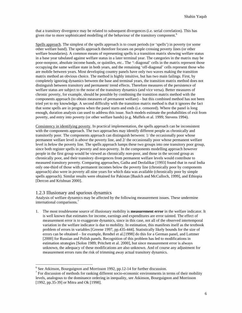
To shed light on the transitory versus permanent distinction, Table 7 shows variability (around intertemporal mean incomes) at different percentiles of intertemporal mean incomes. Thus Table 7 might be taken to show transitory rigidity controlling for permanent welfare levels (some evidence for tail rigidity in the permanent component will be discussed later). In reading Table 7 in this way, it should be noted that any trend changes to permanent income would be taken as transitory variability because of the averaging procedure (especially if it were to vary through the distribution).17 In Pakistan, Sweden, Spain and the USA, the data shows that income fluctuations were considerably larger for those with lower intertemporal mean incomes, suggesting that in these countries chronic poverty and economic insecurity went hand in hand. Bjorklund and Palme [1997] reported that the overall correlation coefficient between intertemporal income variability and intertemporal mean income in Sweden (after taxes and transfers) was negative, i.e. –0.25 for a younger cohort and –0.10 for an older cohort.18 In India, Walker and Ryan [1990] reported the correlation between the intertemporal coefficient of variation of a household’s income and its income level as –0.29, –0.10 and +0.08, depending on study village. Jalan and Ravallion [1998] estimated that in China intertemporal variability in income was similar throughout the distribution, but in contrast, variability in consumption was highest for the richest quartile. Gottschalk [1982] found in the USA a U-shaped relationship between intertemporal earnings variability and intertemporal mean earnings.

Table 7: Transitory fluctuations by ventile of permanent income Country Indicator Period 5 10 15 20 25 30 35 40 45 50 55 60 65 70 75 80 85 90 95 100 SourceSweden: cohort 18-32 yrs old in 1974 Income 1974-91 Bjorklund & Palme '97Sweden: cohort 33-47 yrs old in 1974 1974-91Spain Income 1985-91 Salas & Radan '98USA Earnings 1970-78 Gottschalk and Moffitt '94

1979-87China Consumption 1985-90 Jalan & Ravallion '98

IncomePakistan Income 1987-91 McCulloch & Baulch '990.45 Not reported 0.41

0.080.10

0.520.63

0.590.66

0.500.65

0.510.64

0.030.04 0.03 0.03 0.050.230.34

0.050.05

0.03 0.03 0.03 0.030.08

0.17 0.05 0.02 0.03

0.21 0.07 0.04 0.05

Note: Some results presented as reported by authors, but others derived from data given in the basic source. In terms of tail rigidity in the permanent component, Jarvis and Jenkins [1996] showed that in the UK in the early 1990s, 54 percent of the poorest quintile, and 41 percent of the lowest absolute income class, were immobile after four years.19 Removing some of the transitory element in the dynamics, by looking at mobility in two-year averaged incomes (i.e. comparing ‘income averaged over year one and two’ against ‘income averaged over year three and four’), only indicated higher levels of immobility: 64 percent and 50 percent respectively. This rigidity in the permanent component was greater at the tails than the middle of the distribution, both in relative and absolute transition matrices. Similar results were obtained for the USA, where Hungerford [1993] found that 4.9 percent of the population were in the poorest income decile in both 1979 and 1986, and 5.7 percent were in the lowest absolute income group in both years. Again immobility of income purged of some transitory dynamics (i.e. comparing ‘income averaged over 1977 to 1981’ against ‘income averaged over 1984 to 1988’) was higher: 6.0 percent and 6.8 percent respectively. Both relative and absolute rigidity in the permanent component was greater at the tails compared to the middle of the distribution.20 The evidence is not ideal, but it suggests that at the tails of the distribution rigidity typically combines: 1. relatively lower relative mobility (Table 5), most of which is short-ranged (Table 6), and 2. higher absolute transitory fluctuations (Table 7). Tail rigidity might also include a relatively shallower trend in the permanent component. Such a combination would especially raise concerns over the equality of social opportunity, since it would suggest

17 See for example Iacoviello [1998]. 18 Before taxes and transfers, the figures were –0.39 for both cohorts. 19 Income concept used was post tax and transfers. 20 Identical conclusions applied to an earlier period of 1969 to 1976.

Shahin Yaqub

17

that many of the poorest remain the poorest or nearly-poorest, and much of the mobility they experience reflects their economic insecurity (rather than growth in permanent welfare). This leads to an interesting question: does the fate of developing countries lie in the experiences of rich industrial countries whereby misery – in the form of chronic relative poverty – replaces chronic absolute poverty? Oswald [1997, p.15] found that “economic progress buys only a small amount of extra happiness” as subjectively reported – which largely returns the issue to an earlier fundamental debate over relative versus absolute poverty (see for example, the exchange between Amartya Sen [1983; 1985] and Peter Townsend [1985]). In a more objective sense, being poorest may be stickier than simply being poor. The current view, e.g. Lipton [1997], would be that chronic absolute poverty diminishes with economic growth, but that does not necessarily apply to chronic relative poverty. Table 5 shows that in the USA, even after a period of 22 years (i.e. including much of the life-cycle), 9.4 percent of the population remained in the poorest income quintile. Gaiha [1989] wrote: “What characterises the chronically poor is not so much low per capita income/ expenditure in any year as low variation in it (in absolute terms) over time… due to low/ negligible endowments (e.g. cultivable land, labour power, skills) and/or inability to augment substantially the earnings from them.” The assumption might be that GDP growth would not reduce chronic relative poverty where it leaves untouched inequality in the distribution of human and physical assets, and the returns to assets. Thus a handful of studies have attempted to examine directly mobility in wealth, and life-time income. Table 8 shows that inequality in the long-run component of welfare can be quite high – in several countries Ginis are higher than 0.3 (for comparison, note single year inequality is less than 0.3 in around one-fifth of the countries reported by the World Bank in World Development Indicators 2000). In a village study in Tamil Nadu (India), Swaminathan [1989, 1991] found that 42 percent were in the same quintile of per capita wealth in 1977 and 1985. 21 Of 50 landless households in 1985, 43 (86 percent) were landless also in 1977, two (4 percent) owned under 1 acre, and five (10 percent) owned between 1 and 2.5 acres [Swaminathan 1991b].22 For the USA, Jianakoplos and Menchik [1997] reported that 47 percent were in the same wealth quintile in 1966 and 1981 (78 percent of these household moved only to an adjacent quintile).23 Referring to dynastic command over assets, these results might be assumed to underlie the intergenerational poverty persistence research to be presented later. Jianakoplos and Menchik [1997] uncovered a striking race dimension: in the USA black people were far less likely than white people to escape the lower tail of the wealth distribution, and yet far more likely than white people to move down from the upper tail (see Annex Table 1). This kind of issue is likely repeated in other countries, for example, in India via caste.24 The mean exit time from the lowest wealth quintile for whites was estimated to be 35 years and for blacks 65 years (i.e. basically a lifetime), whereas the mean exit time from the 21 Swaminathan [1989, 1991, 1991b] used gross wealth data in a sample of 458 people in 83 households in a village in Tamil Nadu, India. Wealth included land, agricultural assets, animals, business assets, gold, houses, other buildings, financial assets and consumer durables. Notably, the study did not account for life-cycle effects on household wealth nor debt, though these are likely to have been important. 22 In a small sample of low-income dwellers in Bombay slums, Acharya and Jose [1991, p.51] found that of the 35 male heads of households who first lived on the pavements and 673 in ‘kuccha’ dwellings (of mud, thatch and/or corrugated metal), by the time of the survey, respectively, 37 percent (13 males) and 32 percent (216 males) of them had moved to ‘pukka’ dwellings (of brick and mortar). 23 Jianakoplos and Menchik [1997] was based on USA National Longitudinal Surveys of Mature Men in 1966, 1971, 1976, and 1981 (covering 45-59 year olds at first survey). Wealth was defined as net worth at time of survey (i.e. not including prospective income streams). Sample size was 2218 persons. 24 Lanjouw and Stern [1992] found that the intra- and inter- caste components of the Theil index of inequality in Palanpur (India) had been remarkably stable over a long period of time. The shares of inter-caste inequality in total inequality were 23 percent in 1957/8, 20 percent in 1962/3, 25 percent in 1974/5 and 25 percent in 1983/4 (the balance being attributable to inequality within castes). Lanjouw and Stern concluded “institutions such as caste and share-tenancy retain a powerful role in determining who benefits from economic growth” [p.18]. In reviewing longitudinal village studies in rural India, Jayaraman and Lanjouw [1998] found evidence for a general weakening of restrictions on associations and interactions across castes, and also for some castes, a degree of dissonance between social rankings based on economic conditions and ritual status.

Shahin Yaqub

18

highest wealth quintile for whites was 40 years and for blacks 20 years. Björklund [1993] found that the Gini for the present value of real total income from 1951 to 1989 in Sweden was 0.2 (plus or minus 0.08, depending on age-cohort and choice of discount rate), and this was 35 to 40 percent lower than inequality in single year incomes. Geweke and Keane [2000] estimated for the USA that the standard deviation of the present value of lifetime earnings was $85,400 around a mean level of $131,600 (in 1967 dollars) –such that at the 5th percentile lifetime earnings was 0.29 times the mean, and at the 95th percentile it was 2.2 times the mean. Throughout the distribution, the lifetime earnings of whites was estimated to be around 50 percent greater than blacks’.

Table 8: Inequality in permanent income

Inequality measure Theil0 Theil0Accounting period yr 5 10 6 5 10 5Denmark 0.25 0.22 0.04 0.22 0.20Norway 0.26 0.20Sweden 0.21 0.20 0.17 0.16USA 0.38 0.37 0.16 0.32 0.31France 0.11Germany 0.41 0.36 0.07 0.24 0.21Italy 0.05UK 0.48 0.09 0.28 0.13Netherlands 0.39 0.35 0.25 0.21Hungary 0.27 0.14Spain 0.34

Excluding transfers & taxes Including transfers & taxes

Gini Gini

Source: Gottschalk & Danziger [1997], Galasi [1998], Glewwe & Hall [1998], Maitre & Nolan [1999], Okrasa [1999b], Gaiha [1988], Dercon & Krishnan [2000], Cunningham & Maloney [2000], Skoufias et al. [1999], World Bank [1999b], Maluccio et al. [2000], Randolph & Trzcinski [1989], Jovanovic [2000] Note: Some results presented as reported by authors, but others derived from data given in the basic source. Importantly Geweke and Keane [2000] found that low earnings at age 30 in the USA was a strong predictor of low earnings persistence throughout life, even conditioning on race and education: a white male with under 12 years education in the bottom quintile at age 30 would probably spend 70 percent of his remaining life in the bottom quintile, and a similar black male around 80 percent. Similarly Björklund [1993] also found that single year income inequality in Sweden converges on lifetime income inequality only after age 35 (with a correlation of 0.8): “it is income up to around 30 years of age that mainly accounts for the marked discrepancy between the dispersion of annual and lifetime income”, perhaps due to variations across people in length of education, followed by higher job instability early in a person’s career. Osberg [2000] reported that at least 90 percent of inequality at any given time in Canada, USA, UK, Germany and Sweden was due to differences between people of a similar age (rather than differences in means across age-cohorts). As reported in Annex Table 3, estimates of overall mobility – not just in the permanent component – decline with age. Seebohm Rowntree in 1901 in York (England) found that poverty can follow a life-cycle pattern, but also the more recent evidence suggests that transitory fluctuations may also be lower in later life.25 Underlying these results is the idea that people have characteristics which determine their lifetime income paths (for better, or for worse), and despite some sorting which occurs early in careers, by around middle age people are married to their ‘true’ income path. Thus Geweke and Keane [2000] found that about 60 percent of the variation of lifetime earnings not explained by education and race was attributable to permanent individual characteristics that were unobserved and uncorrelated with education, age and race. Gaiha and Deolalikar [1993] wrote on India: “persistence of poverty is closely linked not just to lack of assets but also to certain innate disadvantages… As such, it identifies households that are poor because of deep-rooted characteristics that cannot be easily changed in the short or medium run, some of which are

25 See for example Kangas and Palme [1998] on life-cycle issues in poverty.

Shahin Yaqub

19

observed, such as schooling of the household head, and others of which are unobserved, such as managerial ability and industriousness. Innately poor households are likely to remain in poverty in spite of such policy interventions as provision or redistribution of physical assets or changes in household size” [p.410-411]. This sorting idea is also consistent with the data on ‘poverty state dependency’ whereby the chances of exiting poverty falls with increasing time in poverty (as does the chances of re-entering poverty with increasing time in non-poverty) – see Table 9. For example in the USA, of those whose time in poverty was longer than four years, nearly 90 percent would remain poor. Generally the chances of escaping poverty are halved by the fifth year in poverty, as compared to the first year in poverty. What might these unobserved characteristics actually be? Usually they are stated as permanent personal traits like intelligence, diligence, reliability, work ethic, etc., and often largely ascribed to genetic endowments or preferences. But plausibly at least some of these characteristics may represent the permanent damage from prior periods in poverty, say in childhood, and may be better treated as endogenous factors. The evidence for suggesting this is postponed until section 3.2 which discusses the role of pre-adult socio-economic background in determining dynamics in the permanent component of welfare.

Table 9: State dependency: % of poor remaining poor after T years of poverty

Poverty line Poorest income quintile

T years poor USA Poland Neth'lds Germany USA UK Germany Canada Spain Hungary1 47 60 32 45 62 53 67 63 24 252 64 72 63 69 74 66 63 73 48 573 73 78 75 65 80 78 52 834 77 80 60 92 685 81 92 58 856 84 91 100 907 85 100 718 87 100 1009 8810 89

Absolute 0.5*median income

Source: Gottschalk & Danziger [1997], Galasi [1998], Glewwe & Hall [1998], Maitre & Nolan [1999], Okrasa [1999b], Gaiha [1988], Dercon & Krishnan [2000], Cunningham & Maloney [2000], Skoufias et al. [1999], World Bank [1999b], Maluccio et al. [2000], Randolph & Trzcinski [1989], Jovanovic [2000] Note: Some results presented as reported by authors, but others derived from data given in the basic source. Spanish estimate for T=2 is actually for T=1.5 years

2.4 Linking mobility to transitory poverty A result of transitory poverty – the result of transitory mobility – is that total poverty is ‘shared’ throughout the population. For example, if in a population of two people there are a total of two years of poverty, are those total poverty years shared equally, one year each (i.e. only transitory poverty exists) – or are they experienced by just one person, one year after the other (i.e. only chronic poverty exists)? Table 10 shows the distribution of years of poverty and nonpoverty, for the years covered in the panels in different countries. For example, 73 percent of the population never experienced poverty in the USA, whereas two percent were always poor – the remainder were transitorily poor for at least one of the years of the ten year panel. Figure 2 shows, for the USA, Pakistan, Zimbabwe and India, the Lorenz curves for the distribution of total years of absolute nationally-defined poverty for the period covered by the panels (obtained through a simple calculation using data in Table 10). The 45-degree line of equality represents a situation where everybody in the population experiences the same amount of time in poverty (which in the USA amounts to 34 days of poverty per year for everybody, 209 days in rural India, 93 days in rural Pakistan, and 135 days in Zimbabwe). All three curves start by running along the x-axis because some proportion of the population never experience poverty. The curves show that of the poverty that exists, it is most unequally distributed in the USA and least in India. Figure 2 serves to illustrate an important choice because one way a country may reduce the incidence of poverty is to shift poverty onto fewer people (i.e. the chronically poor), who then experience all the misery prevailing in a country. Therefore a perverse possibility exists: narrowing economic opportunities to exclude a select few may reduce the head count rate of poverty, as long as the country can tolerate or ignore

Shahin Yaqub

20

the presence of the chronically poor – and yet total misery would not have been reduced. Going back to the earlier two-person example, if poverty was shared equally the poverty incidence would fall from 100 percent of the population in the first year to zero percent in the second year, whereas if it was shifted to just one person, the poverty incidence would remain static at 50 percent. Moreover since the bulk of antipoverty spending increasingly is means-tested or targeted (and so applies only when poverty strikes so as to smooth transitory shortfalls), some kinds of antipoverty spending may have just this effect (of reducing poverty by altering the distribution of total poverty-years in the population) if all it does is stabilise people’s economic welfare into chronic poverty.

Table 10: Percent of population by years of poverty in the period covered by the panel Number of yrs poor 0 1 2 3 4 5 6 7 8 9 10 Source:

USA 73 9 4 3 3 1 2 1 1 1 2 Rodgers & RodgersIndia 12 8 7 5 7 12 7 8 12 22 Gaiha & DeolalikarPakistan 42 24 15 10 7 3 Baulch & McCullochNeth'lds 82 10 3 2 1 2 Muffels et al.UK 82 8 4 3 1 1 Muffels et al.Germany 72 13 7 4 3 2 Muffels et al.Poland 67 15 9 5 3 OkrasaHungary 74 14 6 2 4 Speder in OkrasaZimbabwe 30 27 19 14 11 Baulch & Hoddinott '00Ethiopia 45 30 25 Dercon & Krishnan '00Russia 57 28 13 Mroz & Popkin '95Côte d’Ivoire 61 22 18 Grootaert & Kanbur '95Indonesia 9 16 75 Skoufias et al. '99Note: Some results presented as reported by authors, but others derived from data given in the basic source. Columns add up to 100 percent (except for rounding errors). Poverty defined in absolute terms for all countries, except Netherlands, UK, and Germany

Figure 2: Distribution of total years of poverty in four panels, shown with Lorenz curves

0

10

20

30

40

50

60

70

80

90

100

0 10 20 30 40 50 60 70 80 90 100

Cumulative % of population in panel

Cum

ulat

ive

% o

f yea

rs o

f pov

erty

in p

anel

rural India (Gini=0.70)rural Pakistan (Gini=0.73)USA (Gini=0.94)Zimbabwe (Gini-0.64)Equally shared poverty

Those shown in Table 10 as experiencing more than one year of poverty, may not experience those poor years consecutively. Instead some may ‘churn around the poverty line’. Churning refers to repeated exits and entries across the poverty line. Okrasa [1999b] found that of the population experiencing some time in

Shahin Yaqub

21

poverty over a four year period in Poland, 25 percent experienced entries and exits from poverty and a further 15 percent experienced exits and re-entries into poverty. As already discussed in section 1.2.3 (point 1), identifying true transitory dynamics from measurement error is difficult, and this also makes the extent of churning unclear. Sometimes an arbitrary margin is added to the poverty line to account for measurement errors. Based on different patterns of churning, some authors classify the poor into alternative ‘poverty trajectories’ (see for example, Gardiner and Hills 1999; Walker with Ashworth 1994).

2.5 Linking mobility to inequality, growth, and poverty Due to concerns over comparability, I do not analyse any further the international estimates of mobility collected in this paper. This postpones for example answers to whether unequal countries are any more or less mobile than equal countries; or whether countries which have economic growth are also those with greater mobility; or the relationship between levels of mobility and levels of chronic poverty. This section reports some scattered evidence on these issues, as available in the literature. In Hungary between 1992-96, Galasi [1998, pp.10-11] showed how mobility partially ‘forgave’ rising inequality and massive economic contraction. The Gini increased from 29.3 in 1992 to 30.2 in 1996 (the Theil increased from 15.2 to 18.6), whilst mean income per capita shrank by about 25 percent. But mobility over the period meant that the Gini for ‘incomes aggregated over 1992-6’ was 27.1 (and the Theil was 13.6). The multi-period inequality measures captured the fact that people had better and worse periods from time to time. For the same reason, mean incomes annualised over the five year period declined by a relatively more modest ten percent. Galasi points out: “this is not a general result… the more rapidly subperiod [i.e. cross-sectional] inequality rises over time, the more income mobility is necessary to offset this effect; it is then possible that longer period inequality indices [i.e. inequality in five year aggregated incomes] will become higher as more and more subsequent subperiod incomes are added up”. In other words, inequality rises whenever it outpaces mobility. Gottschalk and Danziger [1997, p.7] make the same point: “increased yearly inequality must be offset by a sufficiently large increase in mobility. The extent of mobility is irrelevant to changes in inequality”. A major cause for concern over rising cross-sectional inequality therefore would be the implied increases in economic insecurity which would be required to offset it. Furthermore, one cannot make statements about changing economic opportunities in Hungary without data on changes in the levels of, and inequality of, the permanent component of incomes. Björklund [1993] reported similar results for Sweden of rising mobility partially counteracting the effect of rising income inequality in the 1980s. Aaberge et al. [1999] found no association between inequality and mobility in earnings (and income) across the USA, Denmark, Norway and Sweden. The USA had the highest earnings inequality by far, and this result remained for inequality in earnings averaged over six years and 11 years – and also for inequality in market income and disposable income. Lengthening the accounting period had only minor effects on inequality differences across countries. This is consistent with findings of Deininger and Squire [1996] that inequality is highly stable through time. The importance of asset inequality within countries for determining income inequality, and its persistence through time, underlie both these findings. Björklund and Jäntti [1997] comparing Sweden and the USA, found no link between intergenerational mobility and inequality.

3 Explaining welfare dynamics

3.1 Socio-economic correlates of mobility

3.1.1 Discussion of methods Attempts to explain welfare dynamics overwhelmingly have relied on correlating observed mobility to socio-economic characteristics. But rather than explaining mobility, these results are best seen as descriptive of the complex data. Instead, they could be read as showing the relationships between multiple

Shahin Yaqub

22

dimensions of welfare (e.g. the chronically poor, in large part but not totally, are the chronically unemployed). Broadly studies identifying mobility correlates suffer methodological shortcomings already encountered in the empirical macroeconomic growth literature (which has a similar motivation, but different unit of analysis). A huge number of variables have been correlated to macroeconomic growth, but the problem is that “variable x1 will soon be found to be significant when the regression includes variables x2 and x3, but it becomes nonsignificant when x4 is included” [Sala-i-Martin 1997, p.178]. Along with more robustness checks along the lines offered in the growth literature (see Sala-i-Martin 1997), more structured models are required which explicitly account for the content and chronology of life-events, before clearer explanations of household and individual mobility are possible. Studies differ in their choice of correlates. These can be classified into variables which are time variant vs. time invariant, predictable vs. unpredictable, and observable vs. unobservable. Time invariant variables are predictable, if not always observable. Of variables which change through time, some might be said to do so fairly predictably and others not. But only some of the variables which affect welfare are observable. Figure 3 illustrates the classification. Each variable type differs in policy relevance. For example, some factors may be completely outside of policy influence (e.g. luck), whereas others may be difficult to affect directly, but may be insurable (e.g. weather). As already discussed (page 19), some time invariant factors actually may be determined at very early stages of a person’s life, and therefore its time invariance may be rather a case of ‘policy arriving too late’. This idea will be returned to in the next section. Other factors may exist which require deeper societal changes, such as removal of discrimination, and these may suffer ‘policy failure’ if the political process is overly myopic. And some factors may be beyond current knowledge, but be open to technological change.

Figure 3 Classification of variables explaining dynamics

ExampleObservable e.g. ageUnobservable e.g. resilience to diseaseObservable e.g. weatherUnobservable e.g. luckObservable e.g. skin colourUnobservable e.g. diligence

Characteristics of variables

Time variantPredictable

Unpredictable

PredictableTime invariant

3.1.2 Summary of results A summary of studies identifying correlates of mobility is shown in Table 11. Bringing together results from different analyses of mobility correlates is difficult due to the variety of definitions, analytical interests, sets of regressors, and estimation strategies. This section focuses on some broad themes, obtained from the results in a highly synthetic fashion. Studies are grouped according to broad mobility concept, although within each group, studies may still differ in the exact definition used for the dependent variable in the regressions. Four mobility concepts are used: 1/ changes in the levels of welfare between two points in time, 2/ shifts between relative welfare bands; 3/ shifts between poverty and nonpoverty statuses, 4/ individual level estimates of transitory and permanent components. Most studies have quite short accounting periods, in which case it might be assumed that a fairly large proportion of the observed mobility is transitory. So the socio-economic characteristics identified therefore largely correlate to transitory dynamics. Those in the fourth group explicitly model transitory and permanent dynamics separately.

Shahin Yaqub

23

Table 11: Summary of studies identifying mobility correlates

Mobility concept Country Accounting period yrs Welfare concept Study

Denmark Aaberge et al.

Norway Aaberge et al.

Sweden Aaberge et al.

USA Aaberge et al.

India, Bombay 4 Earnings Swaminathan '97

Denmark Aaberge et al.

Norway Aaberge et al.

Sweden Aaberge et al.

USA Aaberge et al.

Côte d’Ivoire, urban Grootaert et al. '97

Côte d’Ivoire, rural Grootaert et al. '97

Ethiopia Dercon & Krishnan '00

Indonesia Skoufias et al.

Poland 4 Luttmer '00

Peru Glewwe & Hall

Russia Luttmer '00

South Africa 6 Maluccio et al. '00

Zimbabwe 14 Gross crop income per hhold Hoddinott et al. '99

Mexico 1.25 Cunnigham & Maloney

Ethiopia 2 Dercon & Krishnan '00

El Salvador Conning et al. '00

India, rural Gaiha

Belarus 2 World Bank '96

Poland Okrasa '99

Poland Luttmer '00

Pakistan, rural Baulch & McCulloch '98

Russia Luttmer '00

Chile, rural 18 Income per capita Scott

Netherlands Muffels et al. '99

Germany Muffels et al. '99

UK Muffels et al. '99

Russia 3 Expenditure equivalised World Bank '99

Poland 4 Luttmer '00

Russia 5 Luttmer '00

Hungary 6 Income quintile Galasi '98

Malaysia 10 Male earnings Trzcinski & Randolph '91

USA 5 Quintile income transition Gittleman & Joyce '98

Indonesia 2 Pritchett et al '00

China 6 Jalan & Ravallion '99

India 10 Income per capita Gaiha & Deolalikar '93

4

5

5

Expenditure per capita

Income relative to median

Expenditure per capita

Expenditure per capita

3

Disp income as % of mean income

Earnings as % of mean earnings

Expenditure per capita

Income per capita

5

11

2

5

Changes in levels

Changes in poverty status

Relative mobility

Transitory component

From the results it is possible to identify five sets of mobility correlates: 1/ factors related to labour market experience, 2/ household formation changes, including births, deaths, marriage, and separations, 3/ human capital within the household including education, training, and on the job skills, 4/ physical assets, and 5/ discrimination over race, sex, and caste. The relative importance of these causes of mobility differs from study to study. Several studies note significant regional dummies. On the whole, the impacts of these characteristics followed theoretically predictable directions, such as transitions out of the labour market or reduced labour supply lead to downward mobility, or greater physical capital helped protect against downward mobility. A notable exception is the mixed results over the link between education levels and

Shahin Yaqub

24

mobility. Some studies did find a favourable link with education levels. But also for example, Scott and Litchfield [1994] found that the education level appeared not to play a significant role in determining income levels in 1968, nor income levels in 1986, nor changes in levels between years, nor in ordered probits estimating the probability of upward- downward- or ‘im-’ mobility. Also Trzcinski and Randolph [1991] found that education levels had no effect on the chances of upward relative mobility in earnings for Malaysian males between 1967 and 1976, but it did lower the chances of downward relative mobility. Baulch and McCulloch [1998] found that below a certain income level, education stopped being a significant factor in the chances of upward mobility. One of the more interesting of the results from these studies is the large effect of household demographic change on mobility (labelled as 3 above). Household dissolution through widowhood, divorce, separation, migration, and polygamy lead to welfare changes. Gittleman and Joyce [1998] found that in the USA, divorce increased downward income mobility for women and reduced it for males; on the other hand, marriage had an upward income mobility effect for both sexes, though larger for women – these male-female gaps were shown to have decreased over time since 1968, probably reflecting labour market changes. “[F]or many women becoming a mother is a greater disposing factor to poverty than gender alone… thus the father’s economic relationship with the children is very much a part of the economic portfolio of a woman who is a mother… Given women’s limited economic power relative to men, a non-contributing father in any household type is among the most severe welfare risks mothers and children face” [Bruce and Lloyd 1997, p.221]. In Kinshasa Zaire in 1988, Magnani et al. [1995] found that almost 36 percent fathered children with women other than their current wife or partner. Between one-quarter of women in Asia and North Africa experience widowhood, divorce or separation, and one-third in Latin America and sub-Saharan Africa [Bruce and Lloyd 1997 pp.221]. “Women’s commitment to and need for the family have traditionally been much greater than men’s because basic economic survival and the acquisition of valid social roles have been difficult for women to achieve outside marriage and childbearing. Yet families, even traditional extended ones, do not always provide women with reliable economic protection” [Bruce and Lloyd 1997 pp.220]. Rosenzweig and Stark [1989] hypothesised that in India the marriage of daughters to locationally distant, dispersed yet kinship-related households is a manifestation of implicit interhousehold contractual arrangements aimed at mitigating income risks and facilitating consumption smoothing in an environment characterised by information costs and spatially covariant risks. Analysis of longitudinal South Indian village data lended support to the hypothesis. Marriage plus migration contributed significantly to a reduction in the variability of household food consumption. Farm households afflicted with more variable profits tended to engage in longer-distance marriage plus migration. Some other literature has pointed to the behaviours of women within their relationships to mitigate the consequences of household dissolution risk (e.g. Cain 1986 discusses fertility choices in Bangladesh). Section 3.2 below attempts to relate pre-adult experiences to lifetime mobility. Of course, the poverty of children is just the poverty of their parents, and the socio-economic correlates of parental mobility also underlie transitory and chronic child poverty. This is illustrated for the USA in Table 12. Walker with Ashworth [1994] found that in the USA, whilst 21 percent of children of white household heads experienced at least a spell of poverty by the age of 16, the figure was 79 percent for black children. Also of those experiencing some poverty, 27 percent of black children experienced poverty all or nearly all of their childhoods, as compared to 3 percent amongst white children. Lone parentage increased the risk of at least a spell of poverty from 23 percent to 51 percent for white children, and 49 percent to 93 percent for black children. Parental education reduced the risk of experiencing at least a spell of poverty for white children (from 42 percent to 11 percent); whereas for blacks it had little effect, but it did lower the risk of chronic or permanent poverty (from 19 percent to 1 percent).

Shahin Yaqub

25

Table 12: Poverty experiences by age 16 in USA, according to parental characteristics Transient Occasional Recurrent Persistent Chronic Permanent Prevalence Hhold Head Male 30 8 42 15 8 2 34 Female 16 10 35 9 16 16 76 Yrs in two parent 0-14 yr 23 8 38 14 8 6 63 Family 15 yrs 30 7 45 13 1 2 24 Educ head <12 grade 25 5 46 14 5 5 50 12 grade+ 46 14 24 15 0 0 14 Race White 36 9 38 15 1 2 21 Black 5 7 48 12 15 12 79 Earning rate, head <$10/hr 20 9 47 12 7 6 69 (avg, 1987 prices) >$10/hr 54 6 18 23 0 0 14 Periods head in Always in 39 10 37 13 1 0 24 labour market Some out 17 6 44 15 9 8 72

Source: Walker with Ashworth 1994, p.129, Table 6.4 (adapted) Note: Prevalence is the proportion experiencing a spell of poverty by age 16. First six columns refer to dynamic poverty types (columns total to 100 percent). Transient - a single spell of poverty lasting a single year. Occasional - more than one spell of poverty but none lasting more than one year (in practice the duration of relative prosperity always exceeds the duration of poverty in this cohort). Recurrent - repeated spells of poverty, some separated by more than one year and some exceeding a year in length. Persistent - a single spell of poverty lasting between two and 13 years. Chronic - repeated spells of poverty never separated by more than one year of relative prosperity. Permanent – continuous poverty.

3.2 The ‘silver spoon, plastic spoon’ hypothesis Much of what we understand of ‘poverty’ and ‘economic immobility’ is politically influenced, affecting our definitions of these concepts, language, assumptions, and responses (if any).26 Ideas sharply compete over how society, luck – or alternatively – individual flaw is the leading cause of persistent poverty and economic immobility. This is perhaps especially so when it is ‘poverty amidst affluence’ [Vic and Howards, 1991]. At times both liberals and conservatives have found the notion of an ‘underclass of poor’ unpalatable – conservatives because it contests their belief in society being equal in opportunities, and liberals because sometimes it sounded like victim blaming [Gottschalk et al. 1994]. At the heart of this disagreement is the extent to which a person’s socio-economic background by birth determines the permanent component of economic welfare. It is also implicit in the mysterious set of ‘unobservable factors’ which studies have estimated partly to determine permanent inequality (as reported on page 19, above). Some theories argue that growing up with poor parents implies socio-economic disadvantages which cause poverty and economic immobility in adulthood. Conversely, having rich parents is supposed to provide advantages. This is the ‘silver spoon, plastic spoon’ hypothesis. Some portion of the permanent component of a person’s welfare is thought to be due to these childhood advantages and disadvantages. Therefore whatever transitory circumstances a person faces in a particular period, their chronic poverty or nonpoverty is thought to have been to some extent already determined in childhood. If it were possible to show otherwise, i.e. that socio-economic background has zero effect on permanent welfare, then the political space for antipoverty narrows considerably because in that case the persistently poor, the underclass, the socially excluded and the economically immobile easily become viewed as just the lazy and untalented.

3.2.1 Intergenerational and sibling correlations: reduced form explanations In trying to evaluate the role of childhood in economic opportunities, two indicators commonly used in applied work, could be thought of as representing the many socio-economic characteristics which make up a person’s background: 1/ the permanent component of parental welfare, and 2/ sibling welfare. Both of these can be thought of as highly reduced indicators of a person’s background, meaning that if a single summary indicator of a person’s background were required then the welfare of people that shared that background might be a good start. Intergenerational studies seek to correlate the welfare of offspring to the permanent component of welfare of parents; similarly sibling studies seek to correlate the welfare indicators of siblings. The permanent component of the parent therefore could be interpreted as representing ‘what might have been’ if the same childhood opportunities faced by the parent also prevailed for their offspring. So low parent-offspring correlations in permanent welfare suggest changes in socio-economic opportunities. “A concern for equality of opportunity is apparently one of the main reasons to be interested in intergenerational mobility: our immediate intuitions suggest that more intergenerational 26 For discussion of political influence on poverty discourse see for example Alcock [1997].

Shahin Yaqub

26

mobility means more equal opportunities” [Van de gaer, Martinez, and Schokkaert 1998, p.1]. It is important to bear in mind that the intergenerational literature assesses the links between the permanent component of welfare of parents and their offspring. The literature ignores, or explicitly excludes, any intergenerational effects due to transitory dynamics in parental welfare (e.g. on children’s education), and any intergenerational causes of transitory dynamics in offspring welfare. Sibling correlations utilise the fact that brothers and sisters tend to resemble each other more than a randomly selected pair of non-siblings in terms of genetic makeup, parental socio-economic status, community characteristics, cultural traits, etc.. The extent of correlation across siblings in their welfare levels may be taken to show the impact of socio-economic background. Low welfare correlations between siblings challenges the ‘silver spoon, plastic spoon’ hypothesis. The approach controls for many unobservable factors in a person’s socio-economic background which may affect welfare outcomes. Sibling correlations therefore are stronger tests of the role of background than intergenerational correlations. And an even stronger test – a version of the sibling approach – is to examine correlations between dizygotic twins, and stronger still, correlations between monozygotic twins. But there is an important caveat: as discussed in section 3.3, for a number of well recognised reasons it may be only partially true to say that siblings share similar backgrounds (e.g. biases in parental preferences towards their different offspring, changes in parental socio-economic circumstances between the births of offspring). Intergenerational correlations A regression explaining offspring welfare levels (LHS) with parental welfare levels (RHS) yields two measures of intergenerational mobility – the correlation coefficient R, and the slope coefficient β on the parental variable. The closer β and R are to zero, the less offspring and parental statuses are correlated, and thus the greater the level of intergenerational mobility implied.27 Table 13 and Table 14 report some intergenerational correlation results. The tables report in detail a number of different estimates drawn from each study. This is because estimates are affected by the manner in which certain methodological shortcomings have been addressed, which were apparent in some initial attempts to estimate intergenerational correlations. These earlier estimates, reporting betas under 0.2, are now believed to have been biased downwards due to unrepresentative samples, incorrect estimation of permanent welfare, and not accounting for lifecycle effects.28 Annex Table 3 summarises the biases, and Annex Table 4 indicates how estimates change with methods. Best estimates of betas mostly lie between 0.3 and 0.6, depending on economic indicator, country, period, and methodology. For earnings and incomes, the betas are generally 0.40 or higher. As reported in Table 15, generally lower intergenerational correlations are obtained for wage rates, and income-needs ratios (i.e. material resources divided by a poverty standard). Perhaps a good benchmark for the wide array of estimates presented in the tables are the estimates by Lillard and Reville [1997] – they found in the USA that the intergenerational correlation R in the present value of lifetime earnings was 0.41, and the intergenerational correlation R in the present value of lifetime Duncan index of socio-economic status was 0.47.

27 If the variances of parental and offspring welfare are equal, by definition β and R will be equal 28 Studies simulating earlier methodological problems obtained the earlier low estimates. For example, with simulated ‘data problems’, Solon [1992, p.401] and Zimmerman [1992, p.417] both report β=0.25 for USA father-son earnings; O’Neill and Sweetman [1995, p.21] reports 0.29 for UK father-son earnings; Dearden et al. [1997] reports 0.24 for UK father-son earnings, and 0.35 for UK father-daughter earnings. Their ‘best estimates’ are much higher.

Shahin Yaqub

27

Table 13: Intergenerational income correlations Sample Y=Income X variable R β Source of bias Source Norway Son’s, 1960 Father’s income, 1960 0.11 0.14 2, 3 Soltow in Atkinson

Father’s income 1967 0.48 2, 3 Solon USA Son’s 1984 Father’s education 0.53 IV

Offspring gross inc. c. 1977 Parent’s gross income 1950 0.38 1, 2 Atkinson UK Offspring net inc. c. 1977 Parent’s income net tax 1950 (ln) 0.23 1, 2

Father’s 1974 0.19 2, 3 O’Neill & Sweetman UK Sons’ 1991 Father’s socio-economic 1.00 IV

Sweden Offspring’s 1953 Parent’s income, 1938 0.49 2, 3 Wolff & van Slijpe in Atkinson Son’s 1987 Predicted father’s long run income 0.29 0.36 IV Björklund and Jäntti

Son’s predicted Predicted father’s long run income 0.19 0.24 IV Note: R= correlation coefficient. β= slope coefficient on parental variable. 1 = unrepresentative sampling. 2 = error ridden estimate of long-run status. 3 = no adjustment for life cycle. IV = instrumental variable estimation, treated as addressing both biases 2 and 3.

Table 14: Intergenerational earnings correlations Sample Y=Earnings X variable R β Source of bias Source

Son’s 1965 0.13 Son’s 1966 0.18

USA

Son’s 1967

Parent’s income, avg 1957-60

0.18

1, 3 Sewell & Hauser in Solon ‘92

Sons’ Parent’s income, recalled by son 0.16 2, 3 Bielby & Hauser in Solon ‘92 Offspring’s c. 1979 Father’s earnings c. 1979 0.04 0.07 2, 3 Offspring’s c. 1979 Father’s earnings c. 1979 0.15 0.15 2, 3 Berhman & Taubman

Father’s earnings 1967 0.37 2, 3 Father’s earnings 1971 0.29 2, 3

Father’s earnings avg 1967-71 0.41 3

Son’s 1984

Father’s education 0.53 IV

Solon ‘92

Father’s earnings, yearly 1965-70 0.25 2, 3 Father’s earnings, yearly 1965-70 0.29 2

0.46 3 Father’s earnings, avg 1965-70 0.54

Duncan Index 0.42 IV

Son’s 1981

Fwd quasi-diffce 0.36 IV

Zimmerman

Son’s avg 1981-91 Father’s avg 1981-91 0.28 3 Lillard & Reville Son’s adjusted Father’s adjusted 0.32 Duncan Index Duncan Index 0.44

Father’s earnings 1984 0.09 0.07 2, 3 Father’s earnings 1989 0.16 0.16 2, 3

0.17 0.13 3

USA Son’s avg 1983-8

Father’s earnings avg 1983-8 0.53

Father’s earnings 1984 0.09 0.13 2, 3 Father’s earnings 1989 0.09 0.09 2, 3

0.12 0.11 3

Germany Son’s avg 1983-8

Father’s earnings avg 1983-8 0.52

Couch & Dunn

0.26 0.33 3 Father’s earnings, avg 1967-71 0.31 0.39

Son’s 1987

Predicted father’s long run earnings 0.41 0.52 IV

USA

Predicted son’s Predicted father’s long run earnings 0.26 0.33 IV Son’s 1987 Predicted father’s long run earnings 0.23 0.28 IV Sweden

Predicted son’s Predicted father’s long run earnings 0.17 0.22 IV

Björklund & Jäntti

UK Sons’ 1991 Father’s 1974 0.29 2, 3 Father’s socio-economic 0.64 IV O’Neill & Sweetman

Sons’ 1991 Mid-point father’s earnings class 0.24 2, 3 Son’s 1991 Father’s socio-economic 0.57 IV

Predicted son’s Predicted father’s long run earnings 0.44 IV Daughter’s 1991 Mid-point father’s earnings class 0.35 2, 3 Daughter’s1991 Father’s socio-economic 0.68 IV

Predicted daughter’s Predicted father’s long run earnings 0.51 IV

Dearden et al.

Note: R= correlation coefficient. β= slope coefficient on parental variable. 1 = unrepresentative sampling. 2 = error ridden estimate of long-run status. 3 = no adjustment for life cycle. IV = instrumental variable estimation, treated as addressing both biases 2 and 3.

Shahin Yaqub

28

Table 15: Intergenerational income-needs and wage rate correlations Sample Y variable X variable R β Source of bias Source

Son’s hhold income-needs ratio 1984

Father’s hhold income-needs ratio1967 (ln)

0.48 2, 3 Solon USA

Son’s hhold income-needs ratio 1984

Father’s education 0.56 IV Solon

Father’s hrly wage, yearly 1965-70 0.26 Zimmerman Father’s hrly wage, avg 1965-70 0.37 3 Zimmerman Father’s hrly wage, avg 1965-70 0.39 Zimmerman

Duncan Index 0.49 IV Zimmerman

Son’s hourly wage, 1981

Fwd quasi-diffce 0.38 IV Zimmerman Father’s wage 1967 0.29 2, 3 Solon Son’s wage 1984 Father’s education 0.45 IV Solon

UK Offspring hhold income-needs ratio c. 1977

Parent’s hhold income-needs ratio 1950 0.15 1, 2 Atkinson

Son’s hourly earnings c. 1977 Father’s weekly earnings 1950 0.23 0.44 1, 2 Atkinson Note: R= correlation coefficient. β= slope coefficient on parental variable. 1 = unrepresentative sampling. 2 = error ridden estimate of long-run status. 3 = no adjustment for life cycle. IV = instrumental variable estimation, treated as addressing both biases 2 and 3.

The size of the intergenerational slope coefficient makes a significant difference to an offspring’s prospects. For example, in the USA, a slope coefficient of 0.4 would imply that the probability of a son remaining in the bottom quintile of his distribution, conditional on his father having been at the fifth percentile, would be 0.42 – whereas an intergenerational slope coefficient of 0.2 (i.e. more mobility), lowers the probability to 0.30 [Solon 1992]. O’Neill and Sweetman [1995] found an elasticity of 0.6 for father-son earnings in the UK, and this implies that a son of a father in the top decile would earn twice as much as the son of a father in the bottom decile. Strikingly, this intergenerational advantage in the UK was found to be greater than the earnings advantage in the USA of a college degree over a high school degree (estimated to be 1.7).

The intergenerational transmission effect seems not to be uniform across the income distribution, suggesting a greater prevalence of ‘rags to riches’ than ‘riches to rags’. Consistent with the tail rigidity data presented in section 2.3, the intergenerational literature indicates that offspring of the rich, more rarely become poor. Earnings elasticities, showing the percentage change in son’s earnings for a one percent change in father’s earnings, were almost half for poorer people than richer people. Solon [1992] reported that the elasticity of son’s earnings with respect to father’s earnings in the USA was 0.25 if the father’s log earnings was two standard deviations below the sample mean, 0.35 at the mean, and 0.46 if two standard deviations above the mean. Table 16 illustrates the point using UK data. Offspring of parents in classes 1 and 2 (i.e. respectively, those below the official welfare threshold, and just above it), were more likely to enter class 1 (‘poverty’) than class 5 (‘prosperity’). In contrast, offspring of ‘prosperous parents’ (class 5) had a relative chance of poverty of 0.1. Importantly, Saunders [1997] argues against the use of such odds ratios as a sign of unequal opportunities because: 1/ odds ratios do not take into account differences in ability and motivation between the different groups, and 2/ for odds ratios to improve, the lower class chances for upward mobility would have to improve faster than upper class chances of avoiding downward mobility, and this ignores absolute gains made over time by everybody.

Table 16: Intergenerational poverty transition matrix, UK (% of offspring) Offspring’s income-needs class (brackets show % of poverty threshold) Parent’s income -

needs class 1 (<99%) 2 (100-139%) 3 (140-179%) 4 (180-239%) 5 (>240%)

1 10.5 37.6 18 24.1 9.8

2 10.6 37.6 21.8 22.9 7.1

3 7.9 18.1 24.2 27.1 22.7

4 5.1 21 25.8 21.7 26.4

5 4 22.5 16 27.5 29.9

Total 7.1 26.2 20.8 24.9 20.9

Source: Atkinson et al. (1983, Table 5.5, p.79) Note: Table shows the % of offspring entering each poverty class in 1975-8, for each parental poverty class in 1950. Classes defined in terms of income as % of poverty thresholds used for government transfers – for parents it was the National Assistance (in 1950) and for offspring the Supplementary Benefit (1975-8). Britain does not have an official poverty line, unlike the USA, but Class 1 can be interpreted as the ‘state recognised poor’.

Shahin Yaqub

29

Broader indicators of welfare seem to be more strongly correlated across generations than narrow pecuniary indicators. This may be because they better proxy the permanent component of welfare than incomes and earnings, which have to be statistically adjusted to derive permanent measures. Wealth may be one such long-run indicator. Menchik [1979, p.360] stated that “inheritance of earnings capacity and inheritance of material wealth can reinforce each other to generate more similarity between parent and child wealth [at death] than either of these effects would generate alone”. The estimate for the USA is strikingly high: the simple correlation in parents’ wealth at death (i.e. terminal wealth) with that of offspring’s was R=0.8 [Menchik 1979].29 The elasticity of offspring terminal wealth with respect to parental terminal wealth was 0.76, indicating regression towards the mean in wealth-holding over one generation of about 25 percent. Estimates by others, reported in Behrman and Taubman [1985], are comparable to this: R=0.59 and R=0.71 for USA father-son pairs in the mid-1700s and mid-1800s, and R=0.53 and R=0.60 for UK father-son pairs in the early and middle 1900s. In a sample of rural Indian households, the effect of inheritance of parental wealth on offspring’s wealth creation was negative. An extra rupee inheritance was associated with minus 0.16 rupees net wealth creation by the second generation, and minus 1.08 rupees by the third generation, indicating increasing regression towards the mean such that the third generation adopted fully compensatory behaviour with respect to inheritances [Deolalikar and Singh 1990]. This study suffers from unrepresentativeness of the sample, and errors-in-variables as data was based on recall.30 Lillard and Reville [1997, p.2] found a life-cycle dimension to this in the USA: “correlations in occupational status and prestige are higher than in earnings when the father or son are young, but later in life, intergenerational correlations in earnings converge to estimates for status or prestige”. Occupational status is believed to be a broader welfare measure because it includes nonpecuniary compensation. The intergenerational earnings correlation R was estimated as 0.24 for a younger cohort and 0.33 for an older cohort of sons, the intergenerational correlation R in occupational status was 0.42 for younger sons and 0.44 for older sons, and the intergenerational correlation R in occupational prestige was 0.33 for younger sons and 0.42 for older sons. These results are consistent with results mentioned earlier on p.19 supporting the view that people may go through some initial sorting process before arriving at a true income trend based on their permanent characteristics. Sibling and twin correlations Solon et al. [1991] summarised several sibling correlations from the USA in different periods: for earnings, correlations between brothers ranged from 0.13 to 0.54 (most correlations were at 0.20 or higher), and for incomes from 0.20 to 0.44. Behrman et al. [1980] found in the USA a correlation of 0.24 in the earnings of brothers in 1973, and 0.33 in the earnings of fraternal twins at age 50. Shlonsky [1987] compared the variation in welfare status between brothers relative to the variation between non-brothers. Similarity amongst siblings was highest in welfare assistance, with 62 percent of the variance of this variable explained by membership of a given family. For schooling the corresponding figure was 49 percent, and for occupational prestige 31 percent. Griliches [1979, p.S52] cited work by Taubman et al. based on monozygotic and dizygotic twins in the USA, which estimated that 45 percent of the observed variance in 29 This estimate included adjustment for the possible downward bias arising from the sample including only parental estates exceeding $40,000 (i.e. attenuated range of an independent variable). The unadjusted value was around R=0.5. The sample was derived from probate records in Connecticut USA (N=199). Wealth was recorded at death of parents (sometime in 1930s and 1940s) and deaths of offspring (sometime before 1976). 30 These estimates were based on a household fixed effects model (i.e. differencing equations) to control for intergenerationally persistent, yet unobservable, household characteristics (e.g. propensity to save, or health levels). Lower estimates were obtained without this adjustment: -0.08 rupees for the second generation, and -0.87 rupees for the third generation. Inheritance data was recalled by the third generation in the Village Level Studies (VLS) panel data of the International Crops Research Institute for the Semi-Arid Tropics (ICRISAT), covering 1975/6 to 1984/5 and 400 households from 10 villages in rural south India. Of these, 120 households from three villages were surveyed in each of the nine years. The sample was unrepresentative of rural south India, and its size was 311 households in this study. The fathers’ net wealth was measured at the time of division of property amongst heirs. Son’s net wealth was measured with respect to 1984, with life-cycle effects on wealth creation controlled by including ‘age’ and ‘years as head of household’ variables.

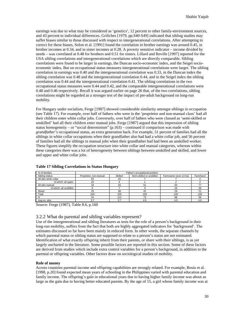
Shahin Yaqub

30

earnings was due to what may be considered as ‘genetics’, 12 percent to other family-environment sources, and 43 percent to individual differences. Griliches [1979, pp.S40-S49] indicated that sibling studies may suffer biases similar to those discussed with respect to intergenerational correlations. After attempting to correct for these biases, Solon et al. [1991] found the correlation in brother earnings was around 0.45, in brother incomes at 0.34, and in sister incomes at 0.28. A poverty sensitive indicator – income divided by needs – was correlated at 0.48 for brothers and 0.51 for sisters. Lillard and Reville [1997] reported for the USA sibling correlations and intergenerational correlations which are directly comparable. Sibling correlations were found to be larger in earnings, the Duncan socio-economic index, and the Seigel socio-economic index. But on occupational status measures intergenerational correlations were larger. The sibling correlation in earnings was 0.40 and the intergenerational correlation was 0.33, in the Duncan index the sibling correlation was 0.48 and the intergenerational correlation 0.44, and in the Seigel index the sibling correlation was 0.44 and the intergenerational correlation 0.41. The sibling correlations in the two occupational status measures were 0.44 and 0.42, and the comparable intergenerational correlations were 0.48 and 0.46 respectively. Recall it was argued earlier on page 26 that, of the two correlations, sibling correlations might be regarded as a stronger test of the impact of pre-adult background on long-run mobility. For Hungary under socialism, Ferge [1987] showed considerable similarity amongst siblings in occupation (see Table 17). For example, over half of fathers who were in the ‘proprietor and non-manual class’ had all their children enter white collar jobs. Conversely, over half of fathers who were classed as ‘semi-skilled or unskilled’ had all their children enter manual jobs. Ferge [1987] argued that this impression of sibling status homogeneity – or “social determinism” (p.163) – continued if comparison was made with grandfather’s occupational status, an extra generation back. For example, 51 percent of families had all the siblings in white collar occupations when their grandfather also had had a white collar job, and 56 percent of families had all the siblings in manual jobs when their grandfather had had been an unskilled worker. These figures simplify the occupation structure into white collar and manual categories, whereas within these categories there was a lot of heterogeneity between siblings between unskilled and skilled, and lower and upper and white collar jobs.

Table 17 Sibling Correlations in Status Hungary % of families Father’s occupational position Sibling status: Proprietor, non-manual Skilled Semi-skilled or unskilled Farmowner (over 13 ha) Farmhand All sibs white collar 53 19 7 7 2

of which: all upper 29 6 1 2 2 All sibs manual 18 43 51 64 77

of which: all unskilled 6 7 9 26 34 Mixed 29 38 42 29 21 Total 100 100 100 100 100 N 34 112 73 88 56 Avg no. sibs 3.7 3.7 4.5 4.5 4.6

Source: Ferge (1987), Table 8.6, p.160

3.2.2 What do parental and sibling variables represent? Use of the intergenerational and sibling literatures as tests for the role of a person’s background in their long-run mobility, suffers from the fact that both are highly aggregated indicators for ‘background’. The estimates discussed so far have been mainly in reduced form. In other words, the separate channels by which parental status or sibling status are supposed to relate to a person’s status are not estimated. Identification of what exactly offspring inherit from their parents, or share with their siblings, is as yet largely uncharted in the literature. Some possible factors are reported in this section. Some of these factors are derived from studies which include extra control variables for a person’s background, in addition to the parental or offspring variables. Other factors draw on sociological studies of mobility. Role of money Across countries parental income and offspring capabilities are strongly related. For example, Bouis et al. [1998, p.20] found expected mean years of schooling in the Philippines varied with parental education and family income. The offspring’s gain in educational years due to having higher family income was about as large as the gain due to having better educated parents. By the age of 15, a girl whose family income was at

Shahin Yaqub

31

the 20th percentile and whose parents both had four years of education, would obtain around 6.8 years of education. This increased by about half a year if either the girl’s family income was at the 90th percentile, or if her parents had ten years of education. And if the girl had both, she would obtain over one extra year. The comparable figures for a 15 year old boy were 5.0 years (base), 6.3 years (income), 6.4 years (parental education), and 7.4 years (income and parental education). The results therefore also showed that rising household income affected boys’ education more than girls’. Filmer and Pritchett [1999] found school enrolment and educational attainment was linked to household wealth in 35 developing countries. The difficulty in the money-outcomes relationship is determining exactly what parental money represents. Parental income could represent greater investment during childhood through greater access to material resources. But quite distinct from this, parental income may just allow better parenting, either by reducing parental stress of not having enough money, or by freeing up time for offspring. And yet parental income may not be the point at all if it is just a proxy for valuable characteristics of parents (such as diligence, reliability, social skills, intelligence etc.), especially if parents are rewarded in the labour market for such characteristics. These issues are important for weighing off the conundrum in maternal paid labour which on the one hand offers greater and intertemporally smoother household income, and on the other hand may result in lower maternal investment of other kinds of inputs into children – evidence for these statements are reported next. These issues relate to a growing literature on time use and household reproduction, in which Folbre [1997] wrote: “A capabilities approach raises a different question, urging us to collect some information about how the capabilities of family members are being developed. In particular, we would want to know how these families organized child care, and what the consequences were for both children and adults.” There is also concern that household reproduction tasks, like obtaining water and fuel, may be more demanding and time-consuming at the same as economic crises lead to extra demands on poor people’s time (e.g. Cooke [1998] for Nepal, Chilimampunga [1997] for Malawi). Evidence from several countries suggests undernutrition adversely affects children’s development across a wide age range, even when controlling for other household characteristics. Food intakes and anthropometric measures have been linked to several developmental areas, including motor, cognitive, mental age, language, socialisation, comprehension, personality, and play behaviours: for example, Upadhyay et al. [1992] for infants in rural India, Sigman et al. [1989] for toddlers in Kenya, Gardner et al. [1999] for toddlers in Jamaica, Aboud and Alemu [1995] for under five year olds in rural Ethiopia, Agarwal et al. [1989] for 6-8 years olds in rural India, and Alderman et al. [1997] for children in rural Pakistan. Alderman et al. [1997] also found stronger negative effects for girls, and Upadhyay et al. [1992] found birth order effects. Gardner et al. [1999] found stunted children showed significantly more apathy, were less happy and were more fussy – nutritional supplementation predicted mental age at 12 and 24 months after enrolment, but had no significant effect on behaviour. Important for this discussion, is the crucial moderating role of maternal attention. Upadhyay et al. [1992], Aboud and Alemu [1995], and Agarwal et al. [1992] all found factors like mother’s involvement in teaching, encouraging the child, or talking to be significant factors. Zeitlin [1991] uses the term “positive deviance” to refer to children who demonstrate above-average growth in impoverished environments. Positive deviants receive more high-quality foods, physical interaction, affection and praise, and verbal and environmental stimulation. Factors that influence child growth through care quality also predict cognitive development, health, and social adjustment. They include the type of society, parental education, mental health, initiative, work burden, family and community structure, and the value of children to parents. Rajan and Jayakumar [1992] reported that a programme in Tamil Nadu (India) in 1982 which provided a daily, free meal to school children aged 2-10 increased school enrolment, and reduced the drop-out rate from 40 percent to 22 percent. Corcoran et al. [1992], whilst controlling for a number of community variables, found parental income in the USA to have a significant positive effect on son’s earnings, and in one equation the elasticity after controlling for observable community characteristics was estimated as 0.37. The proportion of years spent below the poverty line during childhood, whilst living at the parental home, was found to have had large negative and significant effects on son’s earnings, hourly wage, hours of work, income of son’s own family, and income-to-needs ratio. Parental education was found to be insignificant after controlling for parental income, suggesting that the impact of parental education on offspring outcomes is mainly via greater parental income. Datcher-Loury [1989] concluded that variation in academic performance of young children from low-income black families was partly due to differences in parental behaviour and attitudes.

Shahin Yaqub

32

Some families seemed to make the most of its resources (money and time), even if meagre, to increase child quality. This may be through focusing money and time towards children, and through raising family productivity in child quality per unit of resource. Datcher-Loury’s [1989] explanatory variables for academic performance (at ages 6.5 to 7.5, and ages 8.5 to 9.5) included the common indicators for socio-economic status, plus unusually, maternal aspirations for children, and quality of mother-child interactions. Like other children from low income backgrounds, mean test score results on maths and reading were low, and more so for boys (standard deviations range between 25 percent and 40 percent of the mean). But the following results were also obtained. • Different behavioural types of mother-child interaction significantly affected both maths and reading

scores at ages 6.5 to 7.5, but did not have any effect at ages 8.5 to 9.5. Mother-child interactions were measured by four indices (rated during completion of a specified task): 1/ level of affection, 2/ praise for competency, 3/ method of control, 4/ verbal feedback.

• Older ages were significantly affected by educational expectations (in reading, but not maths), and ownership of an encyclopaedia (on both maths and reading). Learning goods, such as books and toys, had significant impacts.

• Mother’s education had a significant positive effect, while father’s did not (except for reading at ages 6.5 to 7.5). Mothers reading to children raised scores significantly, especially for older ages.

Overall, parental behaviour seems to affect reading skills rather than maths, and there is considerable age specificity in the relationship between environment and development. Critically, in maths, gains made at the earlier age were carried forward into later age (which would underline the belief that some capabilities are cumulative through life). Notably, some reverse causality from children’s academic performance and parents behaviour could not be excluded, nor could variations in school quality and other community characteristics. Mayer [1997] employed several strategies for controlling for a range of unobserved parental characteristics, to isolate more closely the effect of income on a range of offspring outcomes during adolescence and at age 24. This focused on the material resource role of money in childhood. Mayer [1997] concluded that parental income had a measurable, though modest, impact on offspring outcomes: “though the effect of parental income on any one outcome appears to be fairly small, higher income has some effect on most outcomes, so its cumulative impact across all outcomes may be substantial” [p.143]. Mayer argued that one of the reasons why the impact may be small is that in the USA the welfare state prevents large material deprivation, beyond which parental characteristics other than income become important in offspring performance. Mayer sees this as a liberal accomplishment, to make parental income less relevant to offspring outcomes, but then points out that this leads to even trickier problems: “children’s opportunities are unequal, [but] income inequality is not the primary reason… if advantage comes from having parents whose depression is treated rather than untreated, from having parents who speak English rather than another language, from having parents who love to read or do math, or parents who love rather than tolerate their children, it will be much harder to equalize opportunity” [p.156]. An important household response to economic insecurity is increased labour supply, especially maternal paid labour (see for example, Rocha [2000] for a review based on ‘national human development reports’, or Cerrutti [2000] for an Argentine study using panel data). There is some evidence to say that children are better protected against consumption shocks if more household income is in their mother’s control. This relies on findings which suggest men and women have different consumption preferences, with women having preferences which are more pro-child, and perhaps also pro-girl (see for example Haddad et al [1996, pp. 48-51]). The obvious implication from this argument is that risks to maternal income pose greater risks for a person’s long-run mobility than risks to paternal income. Thomas [1997] found in Brazil that when income controlled by women increased, household expenditures on health, education and nutrition also increased; and consistent with this, maternal income had a much greater effect on child weight-for-height and height-for-age than paternal income. Moreover, maternal income was found to favour daughters, and paternal income favoured sons. Moreover, Bruce and Lloyd [1997] cited evidence from many countries to indicate that children may obtain better nutritional, educational and anthropometric outcomes in female-headed households, the hypothesis being that women were able to implement more child-friendly resource allocations and behaviours when fully in charge of the household.

Shahin Yaqub

33

The study by Datcher-Loury [1989] cited above found maternal paid work negatively affected scores at the younger age (hypothesised as a time cost), and positively at the older age (hypothesised as a resources gain). Paul-Majumder [1995] looked at the issue in Bangladesh, based on a survey in Dhaka in 1986 of working and non-working women with at least five years schooling and one child under eight years. The study found that employed mothers spent significantly less time with their children in physical child care, tutoring, playing, conversing, etc. compared to non-working mothers – on average nearly 1.5 hours less per day. For working mothers, a greater proportion of the time spent with children was whilst multi-tasking in other household production activities. The study attempted to relate these differences in time-use to different dimensions of human development. For psycho-social development an index was constructed based on teachers’ subjective grading of children to determine aggressiveness (A), moodiness (M) and learning disorders (L) – the AML was significantly better for children over 6 years of working mothers, and no significant differences were obtained for under 6 year olds. Children of working mothers were also found to be more self-sufficient in terms of daily activities, such as cleanliness, eating, homework, etc.. Having a working mother was found to pose no extra risk of morbidity, except possibly for under one year olds (the mean number of times ill in the previous month for under one year olds of working mothers was 1.5, against 1.3 for infants of non-working mothers, with a t-value for the difference in means of 1.85). There appeared to be no large differences between children of working and non-working mothers in terms of the last exam marks (as reported by mother) and current overall school grade (as reported by teacher). Engle [1991], using data from urban Guatemala, tested the hypothesis that during the period of life in which growth often falters (8 through 35 months), maternal employment could be beneficial for children. When poverty and mother’s education were controlled for, no effects of maternal employment on children’s anthropometric growth patterns were seen. However, the percentage of the family income the mother earned was positively associated with all anthropometric indicators, controlling for other factors. Children taken care of by preteen siblings had significantly lower weight for height than those in other situations, even controlling for socio-economic status and maternal employment status. These effects were not found in a sample aged 36-48 months. Jain and Choudhry [1993] found the nutritional status of pre-school children in India to be affected by maternal time on child care activities, maternal working status, and the socio-economic characteristics of the family. Children cared by the mother had better nutritional status than those children who were cared by servants and any other family member in the absence of mother. Tulasidhar [1993] based on Indian census data found that mortality of under 5-year olds was inversely related to maternal education and female labour force participation, but disaggregated analysis showed that female labour force participation had no impact on child mortality among women with fewer than seven years of education. The relative impact of maternal education on child mortality was found to be three times stronger than that of female labour force participation. The incremental savings in child deaths are almost non-existent beyond post-primary maternal education. Very interestingly excess girl mortality prevailing in certain parts of India also had an inverse relationship with the length of mothers’ education, and female labour force participation. Female labour force participation had a stronger influence on excess girl mortality than absolute child mortality. Ricci et al. [1996] studied under five year olds in peri-urban Egypt. Prior to age two, the frequency of feeding was positively related to energy intake, and more time spent in household sanitation activities reduced children’s risk of diarrhoea (during the diarrhoea season). After two years of age, the measured maternal behaviours did not affect children’s energy intake; however, children’s diarrhoeal risk was reduced (during the diarrhoea season) when mothers held them more and allocated more time to household sanitation year-round. The evidence above suggests that where damage from maternal employment occurs, it occurs mostly at early ages. Part of the issue may be the vulnerability of infants to alternative care arrangements (e.g. Hardin et al. [1991] found lower anthropometric indicators amongst children aged 6-12 months).31 Relatedly

31 Gryboski [1996] addresses the manner in which mothers allocate time to infant care as well as to household maintenance and employment. In a longitudinal study with approximately weekly visits between February to June 1991 to 60 infants aged 3-25 months in Central Java, found one or more non-maternal caretaker, mainly grandmothers, sisters, and fathers, provided infant care for 90 percent of the total sample days, and participated in infant feeding on one-third of all sample days. Non-maternal care was on 84 percent of days when symptoms of illness were reported, and fed the infant on 28% of those days. The

Shahin Yaqub

34

Wijekoon et al. [1995] found in rural Sri Lanka maternal employment was significantly associated with a higher risk of formula feeding, whereas the benefits of breastmilk are well recognised. Lactation prevents infant morbidity and mortality due to the immunologic component of maternal milk. Certain antibodies and lymphocytes can be produced by the infant only in later stages of development, and so new-borns must rely on maternal milk for their supply [Stini 1988, p.41]. Apart from direct contributions of antibodies, lactation supplies the infant with cells from the mother which rapidly help the infant to establish its own immune competence. The close proximity of mother and child also ensures that the right kinds of antibodies are produced due to exposure to similar pathogens. Milk production relies on energy and protein consumption by the mother from the second trimester of pregnancy onwards (to build bodily reserves of energy and amino acids), and supplemental energy intake whilst lactating. This means seasonal food shortages will inevitably strike at some point in the pregnancy-lactation period, during which the intake of essential amino acids is the most stringent demand. What happens to the mother at this point would affect infant survival. The point is illustrated in the study by Razzaque et al. [1990] during the 1974-5 famine in Bangladesh. Neonatal mortality risk increased amongst infants conceived, rather than born during the famine (likely impact of gestational malnutrition and maternal health). Post-neonatal mortality risk increased among infants born during the famine, but not amongst the famine-conceived group (likely impacts of maternal malnutrition on breastmilk supply, and early weaning). Second-year mortality risk increased amongst the famine-born (likely impact of debilitation during the famine period). The extra mortality risk from the famine was estimated to dissipate after age 24 months for both famine-born and famine–conceived cohorts, as the more frail members of the cohort died. The poverty status of the household was indicated by a measure of household consumer durables. Poverty had no effect on neonatal mortality, was significant in post-neonatal mortality in the famine-born cohort only, and had significant effects on 12-59 month mortality when all cohorts were pooled. In conclusion, the impact of parental income on offspring outcomes may be country specific, and may be conditioned on the presence or absence of a range of other inputs. This notion of complementarity of inputs has been raised in Lipton et al. [1998]. In developing countries parental income would presumably make more of a direct impact on offspring outcomes. For example, Newman and Gertler [1994] show that in Peru when parents get wage increases, a portion goes towards more consumption, and a portion allows a reduction in the labour supply of children (thereby allowing them more time for activities such as schooling). Studies have also argued that benefits for offspring generally, and girls especially, are maximised where household income is controlled by the mother. Education Considerable evidence exists for intergenerational and sibling correlations in educational outcomes. Filmer [1999] found intergenerational links in 38 countries (and sex and wealth effects in this). Dahan and Gaviria [1999] reported large sibling correlations in educational shortfalls below the median education level in 16 countries in Latin America (ranging from 0.63 to 0.79). Peil [1990] shows how expanding educational systems in Africa has increasingly allowed offspring to attain higher education than their fathers (see Table 18). This tendency is shown to be higher amongst older offspring, with many younger offspring found to have no more education than their fathers. Part of this is due to selective targeting of household resources for education towards some offspring rather than others. “In spite of expanding educational systems, many parents provide no more education for at least some of their children than they got themselves. Decisions are based on the perceived costs of education and opportunities in the labour market as well as children’’ abilities. Girls are particularly disadvantaged…” [Piel p.324].

study findings suggest that health education messages related to infant care and feeding could be usefully targeted to other persons in addition to mothers.

Shahin Yaqub

35

Table 18: Intergenerational Transmission of Education in Africa Father’s Education

None Primary Secondary Percent Nigeria S. Leone Zimbabwe Nigeria S. Leone Zimbabwe Nigeria S. Leone Zimbabwe

Sons None 45 48 26 5 12 1 0 6 0 Primary 30 17 61 23 40 44 3 4 13 Secondary 20 33 13 40 41 54 21 71 80 Higher 5 2 <0.5 32 7 1 76 19 7 Total 100 100 100 100 100 100 100 100 100 N 2390 603 1643 203 757 101 90 45 Daughters None 60 72 31 9 42 2 2 10 0 Primary 22 13 59 28 22 60 11 9 43 Secondary 16 15 10 43 35 38 26 76 57 Higher 2 0 <0.5 20 1 - 61 5 0 Total 100 100 100 100 100 100 100 100 100 N 1581 572 1289 327 157 712 84 101 35

Source: Peil [1990, p.321, Table 3] Note: Cases where father’s education is not known excluded. Primary category includes Koranic schools; secondary includes teachers’ and nursing training. Behrman and Taubman [1985] estimated that the impact on offspring’s education of father’s education is larger than mother’s education, and that whereas the father’s effect is evenly spread between sexes, the mother’s effect is tilted in favour of daughters. Similar results from Malaysia were reported by Lillard and Willis [1994]. But Bouis et al.’s [1998] results for the Philippines were different: the intergenerational impact of maternal education was evenly spread between the sexes of offspring, and paternal education was tilted in favour of boys. In comparison with the USA and UK, Marris argues that Germany has a less spread out distribution of academic performance when children emerge from compulsory education, because children at the lower end perform better (pp.56-7). This point is raised in terms of the idea that, where correctly designed, the education process might compensate for what may be regarded as ‘innate ability’. Similarly, Handa [1996] argues that hopes for greater equality and mobility through greater public investment in education in Jamaica have not been realised. Inequality within education matters, and opportunities for quality education are strongly determined by family and community background. Part of the problem is to understand what exactly education does for a person’s mobility. Gazioglu’s [1994] study on Turkish and Bangladeshi father-son pairs in the UK, indicated that job training, rather than qualifications per se, seemed to have a positive effect on the chances of occupational upward mobility, and this seemed especially so for Bangladeshis rather than Turks.32 Rather than absolute levels of education, some evidence suggests education relative to one’s peers may be an important factor in determining one’s mobility. This would be consistent with credentialist theories of education in the labour process, rather than efficiency theories. It would also appeal to some of the older functionalist explanations of poverty (rooted in the tradition of Durkheim), which sees social stratification and inequality as a way of allocating functions between individuals within society - so that the most talented fill the most important positions, and that there will always be unwanted jobs to be filled at the bottom by the ‘poor’. Similarly Peil [1990] talks about a ‘devaluation of qualifications’ in Africa: “even university graduates may have a hard time finding a job which might formerly have been done by someone with secondary schooling” [p.311]. Gittleman and Joyce [1998] found that in the USA since 1979 poorer income groups did acquire higher absolute levels of characteristics commonly associated with upward mobility (such as education), but these gains were offset by declines in the ‘mobility enhancing impact’ of these characteristics. This is a kind of ‘fallacy of composition’ argument (borrowed from international trade). Kolberg and Kolstad [1993] using a Norwegian panel compared the effect of relative education and absolute education for mobility out of the unskilled service and manual classes over a decade. For a cohort observed in 1960 and 1970, and another in 1970 and 1980, the chances of escape were not much different for the two cohorts even though the latter 32 Interestingly neither father’s occupation nor earnings significantly affected the probability of son’s upward mobility, indicating that “intergenerational upward mobility was not affected by the position of the father on the labour market” [Gazioglu p.349]. This may be a special case for migrants given that first migrants, as pioneers, tend to have taken lower status jobs.

Shahin Yaqub

36

cohort was better educated. Table 19 shows the change in the probability of escape (from unskilled service and manual work) due to the 1.3 year rise in average level of education between 1960 and 1970 (the inter-cohort education gain) compared against the changes in escape probability for somebody having a year more education than the average in their cohort (e.g. intra-cohort education gain). As expected most of the effects are positive, indicating education raises the chances of upward mobility. Where the intra-cohort effect is larger than the inter-cohort effect it is better for upward mobility chances to get more education than one’s peers, than merely gaining the extra year of education by keeping up with their average.

Table 19 Effect of Extra Education on Probability of Upward Mobility from Unskilled Work Long-range mobility Short-range mobility

Sector: Education increased via: Males Females Males Females Inter-cohort gain -4.9 +3.6 +0.7 +5.7 Intra-cohort gain, 1960 +4.5 +1.5 +1.0 +1.8 Consumer services Intra-cohort gain, 1970 +7.9 +3.6 +0.3 +1.5 Inter-cohort gain +4.0 * +7.1 +5.5 Intra-cohort gain, 1960 -0.2 * +0.5 +1.1 Retail services Intra-cohort gain, 1970 +4.6 +3.3 +0.3 +1.2 Inter-cohort gain +9.4 +6.9 -3.2 +5.1 Intra-cohort gain, 1960 +0.9 +2.7 +1.0 +2.4 Social services Intra-cohort gain, 1970 +7.6 +6.4 +0.2 +1.8 Inter-cohort gain +6.2 * +1.0 +9.4 Intra-cohort gain, 1960 +1.4 * +0.7 +2.2 Business services Intra-cohort gain, 1970 +6.9 +1.8 +0.2 +2.0 Inter-cohort gain +0.6 +1.9 -4.0 +5.5 Intra-cohort gain, 1960 +3.7 +0.5 +0.6 +1.2 Manual Intra-cohort gain, 1970 +4.4 +3.0 +0.3 +3.3

Source: author’s calculations based on logit results by Kolberg and Kolstad [1993], pp.64-7 Note: All figures refer to changes in probabilities of upward mobility by unskilled labour, shown for four services sectors and one manual. The mobility can be long-range (into managerial, professional, technical or semi-professional work) or short-range (into skilled work). The 1960 cohort was re-observed in 1970, and the 1970 cohort in 1980. The effect of an inter-cohort education gain is the difference in upward probability for people of average age and average education within each of the cohorts (‘1970’ minus ‘1960’). For males, average age was 33.2 in 1960 and 32.5 in 1970, and average education was 7.5 years in 1960 and 8.8 years in 1970 (an inter-cohort gain of 1.3 years education). For females, average age was 33.6 in 1960 and 32.2 in 1970, and average education was 7.4 years in 1960 and 8.3 years in 1970 (an inter-cohort gain of 0.9 years education). Intra-cohort education gains for the 1960 and 1970 cohorts show the effect on the probabilities of upward mobility for a person having one year more than the average education for their cohort, and with average age. * indicates too few transitions to calculate rates. Culture, class and community Intergenerational and sibling correlations have been shown in class and occupation. Some ideas about ‘culture of poverty’ assumed the poor had distinct social, economic, political, and psychological traits which perpetuate poverty. “Those who argue that jobs and income are the major policy measures for the elimination of poverty are not much interested in culture, but they do make a cultural assumption: that the culture of the poor will not interfere in their adapting to economic opportunity….” [Gans 1970, pp.149-50]. But two problems have long been identified in the non-economic literature with the culture of poverty. First, people’s behaviour patterns may differ from how they would like to behave, because their aspirations may seem unattainable to them, or they may be thwarted by scarce opportunities. Second, behaviour must in some part be due to situational factors and therefore changeable, and this applies even to behaviour patterns which are internalised, and have become part of a person and their community. Townsend [1970] argued that “that the poverty of deprived nations is comprehensible only if we attribute it substantially to the existence of international social stratification, a hierarchy of societies with vastly different resources in which the wealth of some is linked historically and contemporaneously to the poverty of others. This system operated crudely in the era of colonial domination, and continues to operate today, though more subtly, through systems of trade, education, political relations, military alliances and industrial corporations... Second I argued that the poverty of individuals and of families is related to the form of social stratification within nations.” (p.42) In the UK, Indonesia and India between half and two-thirds of samples of offspring were found to have the same class as their parents. Also, the levels of mobility in class were not constant over time. In the UK, Saunders [1997] found 52 percent had changed class from their father’s class at birth.33 In Indonesia, Evers 33 Saunders [1997] used three categories: middle class, working class, and intermediate class. There results were unaffected by using the higher of maternal or paternal class.

Shahin Yaqub

37

and Gerke [1994] found 64 percent were immobile compared to father’s status, 33 percent downwardly mobile, and 40 percent upwardly mobile.34 In India, Saith and Tankha [1992] found immobility in 67 percent of households, upward mobility in 10 percent, and downward mobility in 22 percent.35 In terms of trends in class mobility, Saunders concluded that the chances of working class success in the UK improved - middle-class born children are now 2.2 times as likely as working class-born children to be middle class when aged 33, whereas past research found the figure to be 3 in 1983 and 4 in 1972. Analysing their sample by cohorts aged 16-25, Evers and Gerke [1994] concluded that in Indonesia since 1945, upward mobility rose from 2.8 percent to a peak of 24.8 percent in the 1966-75 cohort, falling to 10.5 percent in the post-1986 cohort - immobility declined, steadied, and then rose slightly to 68.4 percent in post-1986 cohort. 36 In the UK, O’Neill and Sweetman [1998] found that in comparison to sons whose fathers had not been unemployed, sons whose fathers had been unemployed (in either 1969 or 1974) were between two and three times as likely to be unemployed (between 1981 and 1991).37 But if a son experienced unemployment, there was little difference in the time the son spent unemployed, suggesting the impact of father’s unemployment on son’s unemployment history works on incidence of unemployment, rather than duration.38 Couch and Dunn [1996] found the correlation in annual hours worked for father-son pairs in the USA was 0.19 and in Germany 0.17. Imoagene [1989, p.42] showed fast upward occupational mobility after colonial rulers departed, followed by rapid consolidation of position: “almost within a generation, the Nigerian class structure seems to be regimenting itself into cycles of advantage and disadvantage”. Efforts in socialist countries were much more broad based, but were not sustained. “Central authority steps operated in the intended way for a long time to promote long-distance mobility. They involved political and educational means, creation of a new second-chance network of schools, the deliberate reduction or abolition of economic and social privileges and the creation of full employment. But with the consolidation of the structures… the old determinism reappear... Many members of the pre-war upper strata who were effectively deprived of their former privileges and wealth were able to use their non-alienable ‘cultural capital’ to regain, at least for their offspring, part of the loss” [Ferge 1987, p.170]. In a study drawing on research in Bulgaria, Czechoslovakia, GDR, Hungary, Poland, Romania and the USSR, Kolosi and Wnuk-Lipinski [1983, p.3] stated: “Despite every effort at social levelling, various latent inequalities re-emerged. ...if private ownership of the means of production is replaced by collective ownership, some types of inequality are eliminated, some others remain, and some new sorts of inequalities emerge in social life”. One way perhaps to operationalise ‘class’ could be if the classes are spatially concentrated (ghettos? slums? villages?). In that case class would be related to certain measurable variables at the community level. These may be schooling quality, aspirations of peers, availability of information, and access to people to help in securing good jobs. Lacking these market-valued community characteristics raises the opportunity cost to 34 Evers and Gerke [1994] looked at mobility across two classes (upper and lower), amongst wage earners in three areas of Yogyakarta city (the old quarter, a slum, and a semi-rural area). The lower class is defined as those with daily incomes under Rp 5000 and less than primary education (p.3). This corresponds with other studies which have used occupational prestige rankings. Data collection on, and classification of, parental status is not explained in the paper. Sample size was 547 people. 35 Saith and Tankha [1992] combine human and physical wealth to classify 243 households in Uttar Pradesh in 1970 and 1987 into 'rich', 'middle' and 'poor'. They found 42 percent (101 households) poor in both years, 13 percent (32 households) in the middle category in both years, and 12 percent (29 households) rich in both years. This indicates considerable immobility with about 67 percent of households making no class change. Additionally 14 poor landless household left the village. 36 But method and data are not clear in the paper! 37 Using 987 father-son pairs from the National Child Development Study. These estimates hold after controlling for variables likely to affect unemployment history, such as son's human capital. 38 This 'incidence versus duration' result may be because the father variable used in the estimation was an incidence variable (viz. whether unemployed in either 1969 or 1974). Importantly the study excludes children who were of lone-parents, as it includes only children who had both parents present until aged 16. The intergenerational effect may be presumed to be stronger amongst children from disrupted families, since there is evidence that spells into poverty are triggered by family break-ups (e.g. for the USA, Bane and Ellwood 1986).

Shahin Yaqub

38

investing in children. Datcher [1982] attempted to distinguish issues by asking which aspect of a person’s background is important: is it family (to whom one is born) or community (where one is born)? Datcher found that community differences were at least as important as family characteristics in explaining the lower achievements of blacks relative to whites in the USA.39 Similarly, 40 percent of background effect on the gap between the races was due to neighbourhood. In simulations: • if the poorest quartile blacks had the background characteristics of the richest quartile blacks, they

would achieve 0.67 years of extra schooling, and their annual earnings would increase by 30 percent – about 25 percent of the extra schooling and earnings is attributable to the improved community characteristics (the balance to family characteristics);

• if blacks had the background characteristics of whites, blacks would on average have 1.5 years more schooling, with half of this attributable to better community – rather than family – characteristics; also, black annual earnings would rise by about 25 percent, with 40 percent of this attributable to better community characteristics.

Corcoran et al. [1992] undertook a similar exercise, again for the USA. They interpreted ‘welfare dependency’ as capturing the idea of underclass and work disincentives. They found parental welfare receipt or community welfare participation rate have negative effects on son’s: 1/ earnings, 2/ hours of work, and 3/ income-needs. If neighbourhood characteristics are important in determining mobility, then the omission in most poverty analyses of variations in the public provision of goods, especially in developing countries, would be an important one in explaining poverty escape rates.

3.3 Same family but different: intrahousehold biases Interpreting sibling correlations as having controlled for a person’s childhood background characteristics rests on the assumption that siblings actually do share similar socio-economic backgrounds. Relative to people of different parents, this is probably true. Nevertheless the backgrounds of siblings may differ. First, differences may arise due to socio-economic mobility in their family and community in the years intervening between their births. The smaller the age difference between siblings, the more similarity in background expected.40 Second, as discussed below, parents may behave differently towards their different offspring, perhaps according to the sex and parity number of the offspring. In the presence of changing parental circumstances, the sibling correlations reported above could be regarded as lower bound estimates, meaning that the correlations between siblings would be higher if parental circumstances were identical. The same would also apply to most kinds of parental bias (such as between sexes), unless parental biases attempt to compensate offspring for differences in innate ability. Parental bias, if it exists, may be lead to progressive or regressive ‘redistributions’ within the household. If biases are due to simply parental preferences over gender or parity number of their offspring, then it may be better to count such biases as regressive. On the other hand, parents may (knowingly or unknowingly) behave so as to accentuate or attenuate innate differences between siblings, for example by varying schooling or other investments. It may be hard to distinguish the two, but in the latter case, parental bias may be counted as being at least as progressive as say social redistribution. Considerable evidence exists of differential parental treatment of daughters and sons (see for example, Haddad et al. [1997] for a review). For example, Behrman and Deolalikar [1990] found that in semi-arid India male nutrition was protected from price and income shocks. Of total interpersonal variance in nutrition within the sample, intrahousehold variance accounted for between 15 to 48 percent depending on

39 Parents education and aspirations raised son's education, and number of siblings lowered it; parent's income had no effect. For son's earnings, parents income had an effect (positive), and for blacks only, the number of siblings (negative). The neighbourhood characteristic with significant positive effect on both annual and hourly earnings for both blacks and whites was the percent of neighbourhood who were white; notably average neighbourhood income had no effect. Importantly including characteristics of the son, reduced the neighbourhood effects, suggesting that neighbourhood effects worked via sons' characteristics. 40 Rosenzweig and Wolpin [1994] exploit data on changing maternal education levels between sibling births to estimate ‘purer effects’ of maternal education on offspring education. Mayer [1997] attempts a similar exercise with inter-sibling income changes.

Shahin Yaqub

39

nutrient. Food price elasticities for women and girls were estimated to be lower than those for men or boys suggesting that when food prices rise, nutrient intakes by women and girls are adjusted downward by more than the household average. For example, including the impact of significant fixed effects at village, household and individual levels, an average household elasticity of calories with respect to rice price of 0.9, could typically mask elasticities of -0.5 for girls, -0.3 for women, 2.0 for men and 2.4 boys. Despite such persuasive evidence, it should be recalled that most of the evidence on intrahousehold bias relates to parts of South Asia. It is as yet unclear how much gender based parental bias in resource allocations exist in other parts of the world, especially if Haddad et al. [1996, p.37] are correct in suggesting there exists a tendency against publishing ‘negative results’ of no intrahousehold differences. Relatedly Basu [1993] argued that research in South Asia starts with the view that gender differences in nutritional status must exist, although this is not always supported by primary field data.41 Some of literature has speculated that intrahousehold inequality may differ between rich and poor, and also might be related to transitory poverty. Rose [1995] found that in India the bias between girls and boys in survival until school-age (probability of girl-survival divided by the probability of boy-survival) was lower for cohorts experiencing favourable rainfall shocks during the first two years of life – the effect was most pronounced in landless households, indicating girls in poor households with more limited consumption smoothing opportunities appeared to be most vulnerable to shocks. The survival ratio was also related to maternal education and paternal education. Babu et al. [1993] in a study covering six seasons in rural Tamil Nadu, India found that subsistence agricultural households faced less seasonal fluctuations in nutrient intakes than market oriented agricultural households, but also consumed the lowest quantities of energy and protein in all the seasons. Gender bias was greater in protein intakes than energy intakes for all the households, and was greatest in agricultural households. Variations in yields worsened the gender bias. Chakrabarty [1996] found that in West Bengal India, compared to the lean season, the intake of cereal in the peak season was higher, but also the male advantage in net intakes was higher. Rousham [1996] in a longitudinal study of 1366 two-six years olds in rural Bangladesh found biases against girls in anthropometric measures were statistically significant during a period of natural disaster, but became insignificant as conditions improved. This was especially so in landless households. Hardenbergh [1997] in a study of six-nine year olds in the south-eastern rain forest of Madagascar found overall weight-for-height status was worse during the wet season compared to the dry season. Male anthropometric status was worse than that of females during the dry season, but it showed less seasonal variation. The male dietary intake was similar to, or sometimes less adequate than, female dietary intake in the different age cohorts. Leonard [1991] found that under 12 year olds in Andean Peru were protected from seasonal food shortages, with adults carrying the burden during the lean season. This was reflected in skin-fold thickness and weight. Backstrand [1997] in a sample of 246 infants and children in rural Mexico found no girl-boy discrimination in the quantity or quality of food intakes. Nor were gender biases correlated with a crude measure of household consumer durables. The results in a few studies suggest that parents may in certain situations attempt to compensate across differences in their offspring. Behrman [1988] found in India that during the surplus season parents adopted compensating behaviour, giving more nutrients to children with less endowments – nutrients were found to be negatively associated with health indicators. During the lean season however, parents reinforced inequalities by giving more nutrients to children who are better endowed. Larme [1997] studying under 7 year olds over a one year period in northern Puno in Peru, found discrimination against females and younger children, especially infants under age one, despite the fact that these groups were reported to be sicker. Differences were especially significant in the allocation of biomedical treatments, which were the most costly in terms of parental time, effort, and money. Engle and Nieves [1993] on urban Guatemala found no evidence that mothers gave any more food to the child targeted as undernourished by the health centre in a supplementary feeding program. Pitt et al. [1990] found in Bangladesh that households were averse to intrahousehold inequality once linkages between nutrition, labour market productivity, and health 41 For example, Gittelsohn [1991] studying 767 individuals in rural Nepal found no differences in mechanisms of food distribution or nutrient intake between male and female children. Graham [1997] found no gender differences in energy intake or growth among toddlers (one through three years) and preschoolers (four through six years) in the southern highlands of Peru, and that young children do not appear to be deprived of food relative to older household members, especially adults.

Shahin Yaqub

40

heterogeneity were accounted. Dahan and Gaviria [1998] found in the USA that parents reinforce differences in ability of their offspring by investing disproportionately in the most able. Apart from gender, parental resource allocation may also be affected by total family size (i.e. sibling numbers). It is often assumed that more children implies fewer resource availability, and greater competition amongst siblings for resources. Negative correlations have been found between sibling size and offspring outcomes, such as wages, educational attainments, and anthropometric measures (except studies which indicate lower achievements by only-children, as compared to those with one sibling) (see for example, Datcher [1982] and Peil [1990] for reviews). Bohler et al. [1995] found in rural Bhutan that a mother’s subsequent pregnancy had a negative impact on the growth of her last-born child, especially in early pregnancy – reductions of around 28 percent were found in weight and mid-upper-arm circumference. Cochrane et al. [1990] show that in urban Pakistan the number of siblings negatively affected the schooling of girls, but not boys. Studies such as Desai [1995] and Zenger [1992] also showed that the effect of sibling numbers may be conditional on birth spacing (much older siblings may have less of an effect). Moreover, sibling numbers may interact with gender, and it may be that girls from smaller families are more successful than girls from larger families, and the difference between the two may be greater than the corresponding difference for boys. Haddad et al. [1996, p.21] suggested that later-born girls are the most at risk. Kessler [1991, p.421] found that women from small families worked less than women from large families when they were aged 14-22 years, and more when aged 22-30 years. Interestingly for the issues raised in this paper, the family size effect may be larger than certain background characteristics, such as whether the woman had reading material in her childhood [Kessler p.424]. Garg and Morduch [1996] reported that height-for-age and weight-for-height amongst under 15 year olds in Ghana worsened with the total number of siblings, and improved with the number of sisters. Thus children with six siblings of which five were girls showed better anthropometric measures than those with just one sibling. Thus “parents may gain from having sons while children will gain from having sisters… the health of both boys and girls increases with the fraction of their siblings that are female” [Garg and Morduch 1996]. More generally, some literature has focused on fertility.42 “Introducing even a small degree of mobility is an important modification, since it means that persistent higher fertility for the poor will not cause the population to converge to 100% poor” [Lam 1997, p.1038]. Linking mobility to demographic dynamics is very interesting for uncovering effects on mobility common to different cohorts of people, especially where the fertility decision is allowed to be endogenous within the model. The effects of birth order have been harder to determine. Some theories suggest an advantage to earlier-born siblings, and others a later-born advantage (see Harris [1998] for a review). Earlier-born siblings find parents younger, implying fewer risk of birth defects and more energy for parenting; they also compete 42 For example wages have been shown to be related to peer size (Lam 1997, p.1023). Differential fertility across income groups has been cited as a factor in the intergenerational transmission of inequality, because of changing proportions of population in different income groups. How might the steady state proportion of the population in the lowest income class be affected by an increase in the fertility rates of the lowest income class? The is dependent on mobility rates of poor groups relative to non-poor groups. For a given mortality and age structure, the elasticity of the proportion of the population in the poorest class with respect to the reproduction rate of that class is equal to the difference between the probability that a child of poor parents remains poor and the weighted average of the probabilities that children of all other classes become poor, with weights equal to the proportion of the (period t) population born to parents of each class. Thus in the extreme case, an increase in the fertility of the poor will cause a decrease in the proportion poor in the second period, if parents in at least one class are more likely to produce poor offspring than are the poor themselves (i.e. if downward mobility is very high). Lam (1986) applies this approach to Brazilian data to run simulations on the impact of changing fertility, generalising the modelling by including mortality (as well as fertility and mobility- the three together determining changes in population composition) and changes in earnings of the poor relative to others. Whilst clarifying important factors, conclusions from such models less useful for policy than those that relax the exogeneity assumption on fertility decisions (e.g. Raut 1991). Cross-national data has been used to run regressions of inequality against sets of explanatory variables, including demographic variables. The more complicated of these have attempted to allow for endogeneity of demographic variables (e.g. Repetto 1979). Most studies found positive effects of inequality on fertility, and also fertility on inequality.

Shahin Yaqub

41

with fewer demands from other siblings on parental time and whatever resources are available. On the other hand, later-born siblings find parents more mature and experienced (thus enhancing parenting skills), generally financially better-off, and less preoccupied with life; they may also enjoy the benefits of older siblings’ skills and experiences. Birth order may interact with gender, and it may be that the eldest male child is favoured, regardless of his birth order. In practice, correlations have found little relationship between birth order and child achievement. This may simply indicate birth order to be unimportant, or rather, may indicate that birth order has different contradictory effects.

4 Conclusion Sizeable numbers are immobile in absolute terms (the poor staying poor), and even larger numbers are immobile in relative terms (the poorest staying poorest). Clearly some mobility takes place over the life-course, but a lot of mobility is transitory and may just indicate economic insecurity. There may be evidence to say mobility is not uniform across the distribution (less mobility at the tails of the distribution), nor large (most mobility involves small jumps). Intergenerational studies and sibling studies indicate that pre-adult background may have impacts on subsequent lifetime mobility. The channels for this may lie in the impact of parental income, education and social class, but the channels are not straightforward. Coming to some quantitative conclusion on the magnitude of this issue would seem to be vital. If in the extreme case, it turns out that the chances for lifetime mobility are already set solid by the time people become adults, then the window for policy to affect a change would be at far earlier ages than most current antipoverty interventions recognise. The mixed results of active labour market programmes in returning people to work after unemployment may be relevant here [Vodopivec 1999; Terrell and Sorm 1999; Arango and Maloney 2000; van Ours 2000]. If on the other hand, pre-adult background makes a difference but is quantitatively trivial, then focusing on adult opportunities would still be cost-effective. Unfortunately at the moment there is no neat answer to this. But from a human development perspective which tracks the formation and use of capabilities of people from birth to death, it might be noted that the same answers are likely to prevail in developing and industrial countries (i.e. abstracted from questions about whether poverty is ‘different’ in rich and poor countries). The data also suggests that levels and types of mobility might vary within the household along gender and generational lines. But with the thin global coverage of empirical studies, in many contexts women and children may face risks to their welfare which are insufficiently understood.

Shahin Yaqub

42

Annex Table 1: Percentage population in same wealth quintile in 1966 and 1981, USA

Quintile All White BlackPoorest 12 11 15

2 7 7 93 7 7 54 8 8 2

Richest 12 13 5Total 47 46 37

Source: Jianakoplos and Menchik [1997]

Annex Table 2: Life-cycle changes in mobility

<=20 21-25 26-30 31-35 36-40 41-46 46-50 51-56 56-60 61+Shorrocks for Gini after 5 yrs 0.85 0.93Shorrocks for Theil0 after 5 yrs 0.68 0.88Shorrocks for Theil1 after 5 yrs 0.60 0.85Shorrocks for Theil2 after 5 yrs 0.69 0.89

Denmark Earnings Shorrocks for Theil0 after 6 yrsFrance Earnings Shorrocks for Theil0 after 6 yrsGermany Earnings Shorrocks for Theil0 after 6 yrsItaly Earnings Shorrocks for Theil0 after 6 yrsUK Earnings Shorrocks for Theil0 after 6 yrsUSA Earnings Shorrocks for Theil0 after 6 yrs

Transitory Theil0 over 18 yrsTransitory Theil1 over 18 yrsTransitory Theil0 over 18 yrsTransitory Theil1 over 18 yrs

0.73 0.85 0.91 0.91

0.84 0.91 0.900.81 0.85 0.91 0.91

0.46

0.71 0.85 0.91

0.050.413.10

0.070.19

0.52

0.880.750.650.75

0.840.800.83

0.910.810.760.78

0.93

UK

Sweden

0.920.830.800.80

Gross earnings

Market income

Market income detrended

0.29

0.940.75 0.85

0.49

0.910.92

0.88 0.93 0.930.70

Source: Ramos [1999]; Bjorklund and Palme [1997]; OECD [1997] Note: The lower the Shorrocks for a given inequality index, the greater the mobility [Shorrocks 1978].

Annex Table 3: Impact of methodology on intergenerational mobility estimates: theory

Data problem Correlation coefficient, R Slope coefficient,β Unrepresentative sample of parents Downward bias No bias if long-run status

observed, else downward bias

Unrepresentative sample of offspring Downward bias Downward bias Errors in parental status measure Downward bias Downward bias Errors in offspring status measure Downward bias No bias Note: see Solon [1989,1992], Zimmerman [1992], Atkinson et al. [1983, pp.84, 108, 110] for proofs.

Shahin Yaqub

43

Annex Table 4: Impact of methodology on intergenerational mobility estimates: applied

Changes in the range of estimates by type of methodological improvement: Status Measure

Coeff. Basic 1 2 1, 2 1, 2, 3

R 0.04-0.15 0.09-0.16 0.13-0.18 0.12-0.17 0.17-0.53 Earnings β 0.07-0.15 0.07-0.37 0.11-0.46 0.36-0.68 R 0.11-0.49 0.19-0.29 Income β 0.14-0.38 0.19-0.48 0.36-0.53

Income-needs β 0.15 0.48 0.56 Wages β 0.44 0.26-0.29 0.37 0.39-0.49 Source: as stated in Table 14, Table 13, and Table 15 Note: R= correlation coefficient. β= slope coefficient. 1 = more representative sampling. 2 = better estimates of long-run status. 3 = better adjustment for life cycle. Instrumental variables estimation strategy has been treated as serving both improvements 2 and 3, and so where sampling is representative, IV estimates have been included in the final column.

Shahin Yaqub

44

References – Intertemporal Welfare Dynamics

Aaberge, Rolf, Anders Björklund, Markus Jäntii, Mårten Palme, Peder J. Pedersen, Nina Smith, and Tom Wennemo [1999]. Income Inequality and Income Mobility in the Scandinavian Countries Compared to the United States. Working Paper, Department of Economics and Statistics website, Åbo Akademi University

Abul Naga, Ramses H. and Robin Burgess [1997]. Prediction and Determination of Household Permanent Income. Distributional Analysis Research Programme DP32, STICERD London School of Economics

Abumere, S.I. [1981]. “Population Distribution Policies and Measures in Africa South of the Sahara: A Review.” Population and Development Review V7 N3, pp.421-34

Acharya, Sarthi and A.V Jose [1991]. Employment and Mobility: A Study Among Workers of Low Income Households in Bombay City. Asian Regional Team for Employment Promotion [ARTEP], International Labour Office, New Delhi

Adams, Richard H. and Jane J. He [1995]. Sources of Income Inequality and Poverty in Rural Pakistan. Research Report 102, International Food Policy Research Institute, Washington DC

Adetunji, Jacob Ayo [1996]. Infant Mortality and Mother’s Education in Ondo State, Nigeria. Harvard Center for Population and Development Studies

Agarwal, Bina [1997]. “Bargaining and Gender Relations: Within and Beyond the Household.” Feminist Economics V3 N1, pp.1-51

Akszentievics, György [1983]. ‘Mobility and Social Relations.’ In: Tamás Kolosi and Edmund Wnuk-Lipinski, Equality and Inequality Under Socialism: Poland and Hungary Compared. Studies in International Sociology 29, Sage, London

Alcock, Pete [1997]. Understanding Poverty. Macmillan, London

Alderman, Harold and Elizabeth M. King [1998]. “Gender Differences in Parental Investment in Education.” Structural Change and Economic Dynamics V9, pp.453-468

Alderman, Harold and Jere Behrman, Victor Lavy, and Rekha Menon [1997]. Child Nutrition, Child Health, and School Enrolment: A Longitudinal Analysis. Policy Research Working Paper 1700, World Bank, Washington DC

Alderman, Harold and Paul Gertler [1997]. ‘Family Resources and Gender Differences in Human Capital Investments: The Demand for Children’s Medical Care in Pakistan.’ In: Haddad, Lawrence and John Hoddinott and Harold Alderman, Intrahousehold Resource Allocation in Developing Countries. Models, Methods, and Policy. Johns Hopkins, Baltimore

Alderman, Harold and Sudharshan Canagarajah and Stephen Younger [1995]. “A Comparison of Ghanaian Civil Servants’ Earnings Before and After Retrenchment.” Journal of African Economies V4 N2, pp.259-88

Alderman, Harold, and Jere R. Behrman, David R. Ross and Richard Sabot [1996]. “The Returns to Endogenous Human Capital in Pakistan’s Rural Wage Labour Market.” Oxford Bulletin of Economics and Statistics Special Issue: Human Capital in Economic Development, V58 N1, pp.29-57

Allen, Michael Patrick [1980]. ‘The Perpetuation of Wealth: A Simulation Model.’ In: Smith, Modeling the Distribution and Intergenerational Transmission of Wealth. University of Chicago Press, Chicago

Shahin Yaqub

45

Anderson, Mary B. and Peter J. Woodrow [1991]. “Reducing Vulnerability to Drought and Famine: Developmental Approaches to Relief.” Disasters V15 N1, pp.43-54

Arango, Carlos and W.F. Maloney [2000]. Unemployment Dynamics in Latin America: Estimates of Continuous Time Markov Models for Mexico and Argentina. Paper for Annual Bank Conference on Development in Latin America and the Caribbean: ‘Economic Insecurity in LAC’, World Bank, Washington DC

Asthana, Sheena [1995]. “Variations in Poverty and Health Between Slum Settlements: Contradictory Findings from Visakhapatnam, India.” Social Science and Medicine V40 N2, pp.177-88

Atkinson, A.B. [1996]. ‘Seeking to Explain the Distribution of Income.’ In: Hills, New Inequalities: The Changing Distribution of Income and Wealth in the United Kingdom. Cambridge University Press and Joseph Rowntree Foundation

Atkinson, A.B. and A.K. Maynard and C.G. Trinder, with J. Corlyon, S.P. Jenkins and H. Sutherland [1983]. Parents and Children: Incomes in Two Generations. Studies in Deprivation and Disadvantage 10, Heinemann Educational Books, London

Atkinson, A.B. and F. Bourguignon, C. Morrisson [1992]. Empirical Studies of Earnings Mobility. Fundamentals of Pure and Applied Economics 52, Harwood Academic Publishers, Chur, Switzerland

Backstrand, Jeffrey R., and Linsay H. Allen, Gretel H. Pelto, and Adolfo Chavez [1997]. “Examining the Gender Gap in Nutrition: An Example from Rural Mexico.” Social Science and Medicine V44 N11, pp.1751-1759

Bandii, R. and D. Khishigbuyan [1999]. School Drop-outs in Mongolia. Mid-decade Review of Progress Towards Education for All, UNESCO EFA website

Bane, Mary Jo and David T. Ellwood [1986]. “Slipping Into and Out of Poverty: the Dynamics of Spells.” Journal of Human Resources V21 N1, pp.1-23

Barros, Richardo Paes de and Rosane Silva Pinto de Mendonça [1990]. Aggregating Inequalities: The Equalising Impact of the Earnings of Married Women in Metropolitan Brazil. Economic Growth Center Discussion Paper 607, Yale University [also published in 1992 in Sociological Inquiry 62, pp.208-19]

Baulch, Bob and John Hoddinott [2000]. “Economic Mobility and Poverty Dynamics in Developing Countries.” Journal of Development Studies V36 N6, pp.1-24

Baulch, Bob and Neil McCulloch [1998]. Being Poor and Becoming Poor: Poverty Status and Poverty Transitions in Rural Pakistan. Working Paper 79, Institute of Development Studies, Brighton

Begum, Rasheda [1993]. “Women in Environmental Disasters: the 1991 Cyclone in Bangladesh.” Focus on Gender V1 N1, pp.34-40

Behrman, Jere and Paul Taubman [1985]. “Intergenerational Earnings Mobility in the United States: Some Estimates and a Test of Becker’s Intergenerational Endowments Model.” Review of Economics and Statistics V67 N1, pp.144-151

Behrman, Jere R. [1987]. Intrahousehold Allocation of Nutrients and Gender Effects: A Survey of Structural and Reduced Form Estimates. Paper for conference: ‘Poverty, Undernutrition and Living Standards’, 27-31 July 1987, World Institute for Development Economics Research, Helsinki

Behrman, Jere R. [1988]. “Intrahousehold Allocation of Nutrients in Rural India. Are Boys Favoured? Do Parents Exhibit Inequality Aversion?” Oxford Economic Papers V40 N1, pp.32-54

Shahin Yaqub

46

Behrman, Jere R. [1998]. Social Mobility: Concepts and Measurement in Latin America and the Caribbean. Consultant’s report of Februrary 23, 1998 for the Inter-American Development Bank, Washington DC

Behrman, Jere R. and Anil B. Deolalikar [1990]. “The Intrahousehold Demand for Nutrients in Rural South India. Individual Estimates, Fixed Effects, and Permanent Income.” Journal of Human Resources V24 N4, pp.665-696

Behrman, Jere R. and Anil B. Deolalikar [1991]. “School Repetition, Dropouts and the Rates of Return to Schooling: The Case of Indonesia.” Oxford Bulletin of Economics and Statistics V53 N4, pp.467-481

Behrman, Jere R. and Anil B. Deolalikar [1993]. “The Intrahousehold Distribution of Market Labour Supply in Rural South India.” Oxford Bulletin of Economics and Statistics V55 N4, pp.409-421

Behrman, Jere R., and Zdneck Hrubec, Paul Taubman, and Terence J Wales [1980]. Socio-economic Success: A Study of the Effects of Genetic Endowments, Family Environment and Schooling. North-Holland Publishing, Amsterdam

Bender, Deborah E., and Tirsa Rivera and Donna Madonna [1993]. “Rural Origin as a Risk Factor for Maternal and Child Health in Periurban Bolivia.” Social Science and Medicine V37 N11, pp.1345-1349

Besley, Timothy [1995]. “Nonmarket Institutions for Credit and Risk Sharing in Low-Income Countries.” Journal of Economic Perspectives V9 N3, pp.115-127

Bharati, P. and A. Basu [ 1988]. ‘Uncertainties in Food Supply and Nutritional Deficiencies in Relation to Economic Conditions in a Village Population in Southern West Bengal.’ In: Garine, Igor de and Geoffrey Ainsworth Harrison, Coping with Uncertainty in Food Supply. Clarendon Press, Oxford

Bhende, M.J., T.S. Walker, S.S. Lieberman and J.V. Venkataran [1992]. “EGS and the Poor: Evidence from Longitudinal Village Studies.” Economic and Political Weekly V27 No13 (March 28), pp.A19-22

Bird, Edward J. [1995]. “An Exploratory Comparison of Income Risk in Germany and the United States.” Review of Income and Wealth V41 N4, pp.405-426

Birdsall, Nancy, and Thomas C. Pinckney, and Richard H. Sabot [1999]. Inequality, Savings, and Growth. Research Memorandum 148, Center for Development Economics, Williams College

Björklund, Anders [1993]. “A Comparison Between Actual Distributions of Annual and Lifetime Income: Sweden 1951-89.” Review of Income and Wealth V39, N4, pp.377-86

Björklund, Anders and Markus Jäntti [1997]. “Intergenerational Income Mobility in Sweden Compared to the United States.” American Economic Review V87 N5, pp.1009-1018

Blanchflower, David G. and Andrew J. Oswald [1999]. Well-being Over Time in Britain and the USA. Department of Economics website, Warwick University

Bledsoe, Caroline [1990]. “No Success Without Struggle: Social Mobility and Hardship for Foster Children in Sierra Leone.” Man: Journal of the Royal Anthropological Institute of Great Britain and Ireland V25 N1, pp.70-88

Boer, Leen [1981]. Migration and Social Mobility in Bangladesh. Paper for Symposium on Rural Development in South Asia, Intercongress International Union of Anthropological and Ethnological Sciences, April 22-24 1981

Shahin Yaqub

47

Booth, David and Jeremy Holland, Jesko Hentschel, Peter Lanjouw, Alicia Herbert [1998]. Participation and Combined Methods in African Poverty Assessment: Renewing the Agenda. Prepared for the Working Group on Poverty and Social Policy, Special Program of Assistance for Africa, Social Development Division, Department for International Development, London

Bouis, Howarth E., Marilou Palabrica-Costello, Orville Solon, Daniel Westbrook and Azucena B. Limbo [1998]. Gender Equality and Investments in Adolescents in the Rural Philippines. Research Report 108, International Food Policy Research Institute, Washington DC

Bouis, Howarth E., Marilou Palabrica-Costello, Orville Solon, Daniel Westbrook and Azucena B. Limbo [1998]. Gender Equality and Investments in Adolescents in the Rural Philippines. Research Report 108, International Food Policy Research Institute, Washington DC

Brockerhoff, Martin [1995]. “Child Survival in Big Cities: The Disadvantages of Migrants.” Social Science and Medicine V40 N10, pp.1371-1383

Bruce, Judith and Cynthia B. Lloyd [1997]. ‘Finding the Ties that Bind: Beyond Headship and Household.’ In: Haddad, Lawrence and John Hoddinott, Harold Alderman, Intrahousehold Resource Allocation in Developing Countries. Models, Methods, and Policy. Johns Hopkins, Baltimore

Buchanan-Smith, Margaret and Simon Maxwell [1994]. “Linking Relief and Development: An Introduction and Overview.” IDS Bulletin V25 N4, pp.2-17, Institute of Development Studies, Sussex

Burgess, Simon and Carol Propper [1996]. Poverty Dynamics Among Young Americans. Discussion Paper 1362, Centre for Economic Policy Research, London

Burkhauser, Richard V., and Greg J. Duncan, Richard Hauser, and Roland Berntsen [1990]. “Economic Burdens of Marital Disruptions: A Comparison of the United States and the Federal Republic of Germany.” Review of Income and Wealth V36 N4, pp.319-333

Cantó-Sánchez, Olga [1996]. Poverty Dynamics in Spain: A Study of Transitions in the 1990s. Discussion Paper 15, Distributional Analysis Research Programme, STICERD London School of Economics

Carter, Michael R. and Julian May [1999]. One Kind of Freedom: Poverty Dynamics in Post-Apartheid South Africa. Staff Paper 427, Agricultural & Applied Economics website, University of Wisconsin-Madison

Cerrutti, Marcela [2000]. “Economic Reform, Structural Adjustment and Female Labor Force Participation in Buenos Aires, Argentina.” World Development V28 N5, pp.879-891

Chaudhuri, Shubham and Martin Ravallion [1994]. “How Well Do Static Indicators Identify the Chronically Poor?” Journal of Public Economics V53, pp.367-394

Chilimampunga, Charles D. [1997]. “Community’s Survival Mechanisms in Times of Extreme Deprivation.” Community Development Journal V32 N4, pp.312-320

Chowdhury, A. Mushtaque R. and Abbas U. Bhuyia, A. Yusuf Choudhury, and Rita Sen [1993]. “The Bangladesh Cyclone of 1991: Why So Many People Died.” Disasters V17 N4, pp.290-304

Cochrane, Susan, and Valerie Kozel, and Harold Alderman [1990]. Household Consequences of High Fertility in Pakistan. Discussion Paper WDP111, World Bank, Washington DC

Collado, M. Dolores [1998]. “Separability and Aggregate Shocks in the Life-cycle Model of Consumption: Evidence from Spain.” Oxford Bulletin of Economics and Statistics V60 N2, pp.227-249

Shahin Yaqub

48

Conning, Jonathan, and Pedro Olinto, and Alvaro Trigueros [2000]. Managing Economic Insecurity in Rural El Salvador. Paper for Annual Bank Conference on Development in Latin America and the Caribbean: ‘Economic Insecurity in LAC’, World Bank, Washington DC

Corcoran, Mary and Roger Gordon, Deborah Laren and Gary Solon [1992]. “The Association Between Men’s Economic Status and their Family and Community Origins” Journal of Human Resources V27 N4, pp.575-601

Couch, Kenneth A. and Thomas A. Dunn [1997]. “Intergenerational Correlations in Labor Market Status: A Comparison of the United States and Germany.” Journal of Human Resources V32 N1, pp.210-232

Cowell, Frank A., Stephen P. Jenkins, and Julie A. Litchfield [1996]. ‘The Changing Shape of the UK Income Distribution. In: John Hills, New Inequalities: The Changing Distribution of Income and Wealth in the United Kingdom. Cambridge University Press and Joseph Rowntree Foundation

Cox, Donald and Emmanuel Jimenez [1998]. “Risk Sharing and Private Transfers: What About Urban Households?” Economic Development and Cultural Change V46 N3, pp.621-637

Cropper, Maureen L. and Uma Subramanian [1995]. Public Choices Between Lifesaving Programs. How Important are Lives Saved? Policy Research Working Paper 1497, World Bank, Washington DC

Cumpa, Martin and Richard Webb [1999]. Mobility and Poverty Dynamics in the 1990s in Peru. Paper presented at ‘IDS/IFPRI Workshop on Poverty Dynamics’, 7-8 April, Institute of Development Studies, Brighton

Cunningham, Wendy and William F. Maloney [2000]. Measuring Vulnerability: Who Suffered in the 1995 Mexican Crisis? Paper for Annual Bank Conference on Development in Latin America and the Caribbean: ‘Economic Insecurity in LAC’, World Bank, Washington DC

Dahan, Momi and Alejandro Gaviria [1998]. Parental Actions and Siblings’ Inequality. Working Paper 389, Office of the Chief Economist, Inter-American Development Bank, Washington DC

Dahan, Momi and Alejandro Gaviria [1999]. Sibling Correlations and Social Mobility in Latin America. Working Paper 395, Office of the Chief Economist, Inter-American Development Bank, Washington DC

Datcher, Linda [1982] “Effects of Community and Family Background on Achievement” Review of Economics and Statistics V64 N??, pp.32-41

Datcher-Loury, Linda [1989]. “Family Background and School Achievement Among Low Income Blacks” Journal of Human Resources V24 N3, pp.528-544

Davison, J. [1993]. “School Attainment And Gender: Attitudes Of Kenyan And Malawian Parents Toward Educating Girls.” International Journal of Educational Development V13 N4 pp.331-338

Dearden, Lorraine and S. Machin and H. Reed [199?]. Intergenerational Mobility in Britain. Institute of Fiscal Studies, London. [Also as: Discussion Paper 281, Centre for Economic Performance, London School of Economics, 1995]

Dearden, Lorraine and S. Machin and H. Reed [1997]. “Intergenerational Mobility in Britain.” Economic Journal V107 N440 January, pp.47-66

Defo, Barthelemy Kuate [1989]. Mortality and Attrition Processes in Longitudinal Surveys in Africa: An Appraisal of the IFORD Surveys. Working Paper 89-30, Center for Demography and Ecology, University of Wisconsin-Madison

Shahin Yaqub

49

Deininger, Klaus and Lyn Squire [1996]. “A New Dataset Measuring Income Inequality.” World Bank Economic Review V10 N3, pp.565-91

Deininger, Klaus and Pedro Olinto [2000]. Asset Distribution, Inequality and Growth. Policy Research Working Paper 2375, World Bank, Washington DC

Deolalikar, Anil B. and R.P. Singh [1990]. “The Impact of Bequests on Lifetime Wealth Accumulation: An Econometric Study of Two Generations of Rural Households in India.” Review of Income and Wealth V36 N4, pp.353-64

Dercon, Stefan and Pramila Krishnan [1998]. Changes in Poverty in Rural Ethiopia 1989-1995: Measurement, Robustness Tests and Decompositions. Discussion Paper 98-19, Departement Economie, Katholieke Universiteit Leuven

Dercon, Stefan and Pramila Krishnan [1998]. In Sickness and in Health. Risk-sharing Within Households in Rural Ethiopia. Centre for the Study of African Economies website, Oxford University

Dercon, Stefan and Pramila Krishnan [1999]. Poverty, Seasonality and Intra-household Allocation. Paper presented at ‘IDS/IFPRI Workshop on Poverty Dynamics’, 7-8 April, Institute of Development Studies, Brighton

Dercon, Stefan and Pramila Krishnan [2000]. “Vulnerability, Seasonality, and Poverty in Ethiopia.” Journal of Development Studies V36 N6, pp.25-53

Desai, Sonalde [1992]. “Children at Risk: The Role of Family Structure in Latin America and West Africa.” Population and Development Review V18 N4, pp. 689-717

Desai, Sonalde and Devaki Jain [1994]. “Maternal Employment and Changes in Family Dynamics: The Social Context of Women’s Work in Rural South India.” Population and Development Review V20 N1, pp.115-36

Diskin, Patrick [1995]. Understanding Linkages Among Food Availability, Access, Consumption, and Nutrition in Africa. SD Publication Series, Office of Sustainable Development website, Bureau for Africa, USAID Washington DC

Doss, Cheryl R. [1996]. Do Households Fully Share Risk? Evidence from Ghana. Staff Paper P96-10, Department of Applied Economics website, University of Minnesota

Dreze, Jean and Peter Lanjouw and Nicholas Stern [1992]. Economic Mobility and Agricultural Labour in Rural India: A Case Study. Development Economics Research Programme DEP 35, STICERD London School of Economics

Duncan, Greg J., and Björn Gustafsson, Richard Hauser, Günther Schmauss, Hans Messinger, Ruud Muffels, Brian Nolan, and Jean-Claude Ray [1993]. “Poverty Dynamics in Eight Countries.” Journal of Population Economics V6, pp.215-234

Elnur, Ibrahim, and Fatima Elrasheed and Yassir Yacoub [1993]. ‘Some Aspects of Survival: Strategies Among the Southern Sudan Displaced People in Greater Khartoum.’ In: Hans G. Bohle, Thomas E. Downing, John O. Field and Fouad N. Ibrahim, Coping with Vulnerability and Criticality. Freiburg Studies in Development Geography, Verlag Breitenbach, Saarbrucken Germany

Engle, Patrice L., and Sarah Castle and Purnima Menon [1996]. Child Development: Vulnerability and Resilience. Food Consumption and Nutrition Division Discussion Paper 12, International Food Policy Research Institute website, Washington DC

Shahin Yaqub

50

Eriksson, Tor [1997]. Long-term Earnings Mobility of Low Paid Workers. Working Paper 97-16, Centre for Labour Market and Social Research, University of Aarhus

Esping-Andersen, Gøsta [1993]. ‘Post-industrial Class Structures: An Analytical Framework.’ In: Esping-Andersen, Gøsta, Changing Classes. Stratification and Mobility in Post-industrial Societies. Studies in International Sociology 45, Sage, London

Evers, Hans-Dieter and Solvay Gerke [1994]. Social Mobility and the Transformation of Indonesian Society. Working Paper 202, Sociology of Development Research Centre, Faculty of Sociology, University of Bielefeld, Germany

Ferge, Zsuzsa [1987]. ‘The Dynamics of the Reproduction of Social Relations.’ In: Ferge, Zsuzsa and S.M. Miller, Dynamics of Deprivation. Gower, England

Ferge, Zsuzsa and S.M. Miller [1987]. ‘Social Reproduction and the Dynamics of Deprivation.’ In: Ferge, Zsuzsa and S.M. Miller, Dynamics of Deprivation. Gower, England

Ferranti, David de, and Guillermo E. Perry, Indermit S. Gill, Luis Servén, with Francisco H.G. Ferreira, Nadeem Ilahi, William F. Maloney and Martin Rama [2000]. Securing Our Future in a Global Economy. World Bank, Washington DC

Fields, Gary S. [1998]. Income Mobility: Meaning, Measurement and Some Evidence for the Developing World. Paper for the ‘Workshop on Social Mobility’, June 1998, Brookings Institution, Washington DC

Filmer, Deon [2000]. The Structure of Social Disparities in Education: Gender and Wealth. Policy Research Working Paper 2268, World Bank, Washington DC

Filmer, Deon and Lant Pritchett [1999]. The Effect of Household Wealth on Educational Attainment: Evidence From 35 Countries. Population and Development Review V25 N1, pp.85-120

Fiske, Edward B. [1998]. Wasted Opportunities: When Schools Fail. Repetition and Drop-out in Primary Schools. Education for All Status and Trends website, UNESCO

Fofack, Hippolyte and Albert Zeufack [1999]. Dynamics of Income Inequality in Thailand: Evidence from Household Pseudo-Panel Data. Mimeo (seminar paper), World Bank, Washington DC

Folbre, Nancy [1997]. A Time (Use Survey) for Every Purpose: Non-market Work and the Production of Human Capabilities. Paper for the on ‘Time Use, Non-market Work and Family Well Being’, 22-21 November, Washington DC

Foster, Andrew D. [1994]. “Poverty and Illness in Low Income Rural Areas.” American Economic Review V84 N2, pp.216-220

Foster, Andrew D. [1995]. “Prices, Credit Markets and Child Growth in Low-Income Rural Areas.” Economic Journal V105 N430, pp.551-570

Foster, James, and Joel Greer and Erik Thorbecke [1984]. “A Class of Decomposable Poverty Measures.” Econometrica V52 N3, pp.761-766

Frankenberg, Elizabeth and Duncan Thomas and Kathleen Beegle [1999]. The Real Costs of Indonesia’s Economic Crisis: Preliminary Findings from the Indonesian Family Life Surveys. Working Paper, RAND Corporation USA

Gaiha, Raghav [1988]. “Income Mobility in Rural India.” Economic Development and Rural Change V36 N2, pp.279-302

Shahin Yaqub

51

Gaiha, Raghav [1989]. “Are the Chronically Poor Also the Poorest in Rural India?” Development and Change V20, pp.295-322.

Gaiha, Raghav [1996]. “How Dependent are the Rural Poor on the Employment Guarantee Scheme in India?” Journal of Development Studies V32 N5, pp.669-694

Gaiha, Raghav and Anil B. Deolalikar [1993]. “Persistent, Expected and Innate Poverty: Estimates for Semi-Arid Rural South India.” Cambridge Journal of Economics V17 N4, pp.409-421

Galasi, Péter [1998]. Income Inequality and Mobility in Hungary 1992–1996. Innocenti Occasional Paper 64, UNICEF Florence

Gans, Herbert [1970]. ‘Poverty and Culture: Some Basic Questions About Methods of Studying Life-Styles of the Poor’ In: Peter Townsend, The Concept of Poverty. Heinemann, London

Garg, Ashish and Jonathan Morduch [1996]. Sibling Rivalry, Resource Constraints, and the Health of Children: Evidence from Ghana. Development Discussion Paper 553, Harvard Institute for International Development

Garine, Igor de and Geoffrey Ainsworth Harrison [1988]. Coping with Uncertainty in Food Supply. Clarendon Press, Oxford

Garza, Gustavo [1996]. “Social and Economic Imbalances in Metropolitan Area of Monterrey.” Environment and Urbanisation V8 N2, pp.31-42

Gazioglu, Saziye [1994]. “Turkish and Bangladeshi Fathers and Sons in the London Labour Market.” METU Studies in Development [Ankara] V21 N3, pp.341-365

Geweke, John and Michael Keane [2000]. “An Empirical Analysis of Earnings Dynamics Among Men in the PSID: 1968-1989.” Journal of Econometrics V96, pp.293-356

Giddens, Anthony [1998]. The Third Way. The Renewal of Social Democracy. Polity Press, Cambridge

Gittleman, Maury and Mary Joyce [1998]. Have Family Income Mobility Patterns Changed? Paper presented at the 25th General Conference of the International Association for Research on Income and Wealth, August 1998, Cambridge, England

Glewwe, Paul and Gillette Hall [1995]. Who is Most Vulnerable to Macroeconomic Shocks? Hypotheses Tests Using Panel Data from Peru. Living Standards Measurement Study Working Paper 117, World Bank, Washington DC

Glewwe, Paul and Jacques van der Gaag [1990]. “Identifying the Poor in Developing Countries: Do Different Definitions Matter?” World Development V18 N6, pp.803-814

Glick, Peter and David E. Sahn [1998]. “Maternal Labour Supply and Child Nutrition in West Africa.” Oxford Bulletin of Economics and Statistics V60 N3, pp.325-357

Goetz, Ann Marie and Rina Sen Gupta [1996]. Who Takes the Credit? Gender, Power, and Control Over Loan Use in Rural Credit Programs in Bangladesh. World Development V24 N1, pp. 45-63

Goldin, Liliana R. [1996]. “Economic Mobility Strategies Among Guatemalan Peasants: Prospects and Limits of Non-traditional Vegetable Cash Crops.” Human Organization: Journal of the Society for Applied Anthropology V55 N1, pp.99-107

Shahin Yaqub

52

Goodman, Alissa and Steven Webb [1995]. UK Income Distribution 1961-1991. Institute for Fiscal Studies, London

Gottschalk, Peter [1982]. “Earnings Mobility: Permanent Changes of Transitory Fluctuations?” Review of Economics and Statistics, August, pp.450-6

Gottschalk, Peter and Sheldon Danzinger [1997]. Family Income Mobility - How Much is There and Has it Changed? Boston College website, USA

Gottschalk, Peter, Sara McLanahan and Gary D. Sandefur [1994]. “The Dynamics and Intergenerational Transmission of Poverty and Welfare Participation.” In: Sheldon H. Danziger, Gary D. Sandefur, and Daniel H. Weinberg, Confronting Poverty: Prescriptions for Change. Sage, New York

Government of Bangladesh and Asian Development Bank [1996] Study of Urban Poverty in Bangladesh. Final Report: Volume 1. Survey Results. Planning Commission, Govt. of Bangladesh, Dhaka

Government of Bangladesh and Asian Development Bank [1996b] Study of Urban Poverty in Bangladesh. Final Report: Volume 2. Policy Papers. Planning Commission, Govt. of Bangladesh, Dhaka

Greene, William H. [1997]. Econometric Analysis. Third Edition, Prentice Hall

Griliches, Zvi [1979]. “Sibling Models and Data in Economics: Beginnings of a Survey.” Journal of Political Economy V87 N5 Part 2, pp. S37-S64

Grootaert, Christiaan and Ravi Kanbur [1995]. “The Lucky Few Amidst Economic Decline: Distributional Change in Côte d’Ivoire as Seen Through Panel Data Sets, 1985-88.” Journal of Development Studies V31 N4, pp.603-619

Grootaert, Christiaan and Ravi Kanbur and Gi-Taik Oh [1997]. “The Dynamics of Welfare Gains and Losses: An African Case Study.” Journal of Development Studies V33 N5, pp.635-657

Grootaert, Christiaan with Lionel Demery and Ravi Kanbur [1996]. Analyzing Poverty and Policy Reform. The Experience of Côte d’Ivoire. Avebury, Aldershot

Gross, Rainer, and Britta Landfried, Susilowati Herman [1996]. “Height and Weight as a Reflection of the Nutritional Situation of School-aged Children Working and Living in the Streets of Jakarta.” Social Science and Medicine V43 N4, pp.453-458

Gunning, Jan Willem, and John Hoddinott, Bill Kinsey and Trudy Owens [2000]. “Revisiting Forever Gained: Income Dynamics in the Resettlement Areas of Zimbabwe, 1983-96.” Journal of Development Studies V36 N6, pp.131-154

Haddad, Lawrence and Christine Peña, Chizuru Nishida, Agnes Quisumbing, and Alison Slack [1996]. Food Security and Nutrition Implications of Intrahousehold Bias: A Review of Literature. Discussion Paper 19, Food Consumption and Nutrition Division website, International Food Policy Research Institute, Washington DC

Haddad, Lawrence, and John Hoddinott and Harold Alderman [1997]. Intrahousehold Resource Allocation in Developing Countries. Models, Methods, and Policy. Johns Hopkins, Baltimore

Handa [1996]. “The Determinants of Teenage Schooling in Jamaica: Rich vs. Poor, Females vs. Males.” Journal of Development Studies V32 N4, pp.554-580

Hanushek, Eric A. and Victor Lavy [1994]. School Quality, Achievement Bias, and Dropout Behavior in Egypt. Living Standards Measurement Study Working Paper 107, World Bank, Washington DC

Shahin Yaqub

53

Harris, Judith Rich [1998]. The Nurture Assumption. Why Children Turn Out the Way They Do. Bloomsbury, London

Harrison, Geoffrey Ainsworth [1988]. ‘Seasonality and Human Population Biology.’ In: Garine, Igor de and Geoffrey Ainsworth Harrison, Coping with Uncertainty in Food Supply. Clarendon Press, Oxford

Hauser, Richard and Holger Fabig [1999]. “Labor Earnings and Household Income Mobility in Reunified Germany: A Comparison of the Eastern and Western States.” Review of Income and Wealth V45 N3, pp.303-324

Herring, Ronald J. [1998]. Agrarian Reform, Path Dependency and Persistent Poverty: Lessons from the United States and India. Paper for the conference ‘What Can Be Done About Poverty?’, 29 June, Institute of Development Studies, Sussex

Hill, R.D. and Voo Min Shin [1990]. “Occupational and Spatial Mobility in an Overseas Chinese Agricultural Community: The Hakkas of Kudat, Sabah, Malaysia.” Sojourn: Journal of the Institute of Southeast Asian Studies, Singapore V5 N2, pp.194-218

Hoa, D.P. and B. Höjer and Lars Å. Persson [1997]. “Are There Social Inequities in Child Morbidity and Mortality in Rural Vietnam.” Journal of Tropical Pediatrics V43 N4, pp.226-231

Hobcraft, John [1993]. “Women’s Education, Child Welfare and Child Survival: A Review of the Evidence.” Health Transition Review V3 N2, pp.159-74

Hubbard, Michael [1995]. Improving Food Security. A Guide for Rural Development Managers. Intermediate Technology Development Group, London

Hungerford, Thomas L. [1993]. “U.S. Income Mobility in the Seventies and Eighties.” Review of Income and Wealth V39 N4, pp.403-417

Iacoviello, Matteo [1998]. Inequality Dynamics: Evidence from Some European Countries. Working Paper 191, Luxembourg Income Study website

Imoagene, O. [1989]. “Social Origins and Occupational Mobility in a Dependent Society.” Nigerian Journal of Sociology V1 N1, pp.34-49

Isiugo-Abanihe, Uche C. Child Fosterage in West Africa. Population and Development Review, V11 N, March 1985, pp. 53-73

Islam, Nabiul K.M. [1997]. Potential Indirect Impacts of Flooding on Health. Evidence from Macrolevel Data on the Incidence of Disease in Bangladesh. Research Report 155, Bangladesh Institute of Development Studies, Dhaka

Jalan, Jyotsna and Martin Ravallion [1998]. “Transient Poverty in Postreform Rural China.” Journal of Comparative Economics V26, pp.338-357

Jalan, Jyotsna and Martin Ravallion [1999]. Do Transient and Chronic Poverty in Rural China Share Common Causes? Paper presented at ‘IDS/IFPRI Workshop on Poverty Dynamics’, 7-8 April, Institute of Development Studies, Brighton – a version of this is in Journal of Development Studies V36 N6, pp.82-99

Jalan, Jyotsna and Martin Ravallion [1999b]. “Are the Poor Less Well Insured? Evidence on Vulnerability to Income Risk in Rural China.” Journal of Development Economics V58 N1, pp.61-82

Jarosz, Maria [1987]. ‘Intergenerational Trends in Deprivation and School Careers.’ In: Ferge, Zsuzsa and S.M. Miller, Dynamics of Deprivation. Gower, England

Shahin Yaqub

54

Jarvis, Sarah and Stephen P. Jenkins [1996]. Changing Places: Income Mobility and Poverty Dynamics in Britain. Working Paper 96-19, Centre on Micro-Social Change website, Essex University

Jarvis, Sarah and Stephen P. Jenkins [1998]. “How Much Income Mobility is There in Britain?” Economic Journal V108 N? March, pp.428-443

Jaspers, Susanne and Helen Young [1995]. “Malnutrition and Poverty in the Early Stages of Famine: North Darfur, 1988-90.” Disasters V19 N3, pp.198-215

Jayaraman, Raji and Peter Lanjouw [1998]. The Evolution of Poverty and Inequality in Indian Villages. Policy Research Working Paper 1870, World Bank, Washington DC

Jayaweera, Swarna and Thana Sanmugam [1993]. Employment and Occupational Mobility Among Women in Manufacturing Industries of Colombo, Sri Lanka. Asian Regional Team for Employment Promotion [ARTEP], International Labour Office, New Delhi

Jenkins, Stephen P. [1998]. Modelling Household Income Dynamics. Paper for the Twelfth Congress of the European Society for Population Economics, June 1998, Centre on Micro-social Change website, University of Essex (forthcoming in Journal of Population Economics)

Jianakoplos, Nancy A. and Paul L. Menchik [1997]. “Wealth Mobility.” Review of Income and Statistics V? N?, pp.18-31

Johnson, Paul and Gary Stears [1998]. “Why are Older Pensioners Poorer?” Oxford Bulletin of Economics and Statistics V60 N3, pp.271-291

Jovanovic, Branko [2000]. Russian Roulette – Expenditure Inequality in Russia, 1994-1998. Department of Economics, Texas A&M University

Kangas, Olli and Joakim Palme [1998]. Does Social Policy Matter? Poverty Cycles in OECD Countries. Paper presented at 14th World Congress of Sociology, July 26th 1998, Montreal (on Luxembourg Income Study website)

Kessler, Daniel [1991]. “Birth Order, Family Size, and Achievement: Family Structure and Wage Determination.” Journal of Labor Economics V9 N4, pp.413-426

Kinsey, Bill and Kees Burger and Jan Willem Gunning [1998]. “Coping with Drought in Zimbabwe: Survey Evidence on Responses of Rural Households to Risk.” World Development V26 N1, pp.89-110

Kirui, Paul Martin Kipngetich [1982]. A Study of the Factors that Influence the Increasing Repetition and Dropout Rates in Primary Schools in Nandi District of Kenya. African Studies in Curriculum Development & Evaluation 67

Kolberg, Jon Eivind and Arne Kolstad [1993]. ‘Post-industrial Stratificational Order: The Norwegian Experience.’ In: Esping-Andersen, Gøsta, Changing Classes. Stratification and Mobility in Post-industrial Societies. Studies in International Sociology 45, Sage, London

Kolosi, Tamás and Edmund Wnuk-Lipinski [editors, 1983]. Equality and Inequality Under Socialism: Poland and Hungary Compared. Studies in International Sociology 29, Sage, London

Kool, Maarten L. and Dik Verboom and Jan J. Van der Linden [1989]. Mid-term Impacts of Squatter Settlement Upgrading. A Longitudinal Study of Baldia Township, Karachi. Urban Research Working Paper 21, Free University, Netherlands

Shahin Yaqub

55

Krishnan, Pramila [1996]. “Family Background, Education and Employment in Urban Ethiopia.” Oxford Bulletin of Economics and Statistics Special Issue: Human Capital in Economic Development, V58 N1, pp.167-185

Kuch, Priscilla Joseph [1993]. ‘Food Situation Among Displaced Sudanese in Khartoum State.’ In: Hans G. Bohle, Thomas E. Downing, John O. Field and Fouad N. Ibrahim, Coping with Vulnerability and Criticality. Freiburg Studies in Development Geography, Verlag Breitenbach, Saarbrucken Germany

Lam, David [1988]. “Marriage Markets and Assortative Mating with Household Public Goods: Theoretical Results and Empirical Implications” Journal of Human Resources 23, pp.462-487

Lam, David [1997]. ‘Demographic Variables and Income Inequality.’ In: M.R. Rosenzweig and O. Stark, Handbook of Population and Family Economics, Elsevier Science B.V

Lanjouw, Peter and Nicholas Stern [1991]. “Poverty in Palanpur.” World Bank Economic Review V5 N1, pp.23-55

Lanjouw, Peter and Nicholas Stern [1993]. ‘Agricultural Changes and Inequality in Palanpur, 1957-84.’ In: K. Hoff, A. Braverman, and J.E. Stiglitz, The Economics of Rural Organisation: Theory, Practice, and Policy. Oxford University Press, Oxford

Layte, Richard, and Bertrand Maitre, Brian Nolan, and Christopher T. Whelan [1999]. Income Deprivation and Economic Strain: An Analysis of the European Community Household Panel. Working Paper 5, European Panel Analysis Group, University of Essex

Lee, W. O. [1998]. Equity and Access to Education in Asia: Levelling the Playing Field. International Journal of Educational Research V29 N7, pp.667-683

Leeuwen, Jolanda van [1998]. To Work Oneself out of Poverty: the Dutch Experience 1989-1995. Paper for the 25th General Conference of the International Association for Research in Income and Wealth, 23-29 August, Cambridge, England

Leonard, William R. [1991]. “Household-level Strategies for Protecting Children from Seasonal Food Scarcity.” Social Science and Medicine V33 N10, pp.1127-1133

Lewis, Arthur W. [1972]. ‘Reflections on Unlimited Labour.’ In: Luis Eugenio Di Marco, International Economics and Development: Essays in Honour of Raul Prebisch,

Lillard, Lee A. and Robert T. Reville [1997]. Intergenerational Mobility in Earnings and Occupational Status. RAND, California

Lipton, Michael, with Shahin Yaqub and Eliane Darbellay [1998]. Successes in Anti-poverty. International Labour Office, Geneva

Lloyd, Cynthia B. and Anastasia J. Gage-Brandon [1994]. “High Fertility and Children’s Schooling in Ghana: Sex Differences in Parental Contributions and Educational Outcomes.” Population Studies V48 N2, July, pp.293-306

Luttmer, Erzo F.P [2000]. Inequality and Poverty Dynamics in Transition Economies: Disentangling Real Events from Noisy Data. Background paper for ‘Making Transition Work for Everyone: Poverty and Inequality in Europe and Central Asia’, World Bank, Washington DC

Maforah, Fidelia [1994]. “Impact of Poverty on Health in Urbanising Communities.” Journal of Social Development in Africa [Zimbabwe] V9 N2, pp.87-100

Shahin Yaqub

56

Magnani, Robert J., and Jane T. Bertrand, Bakutuvwidi Makani, Stacy W. McDonald [1995]. “Men, Marriage and Fatherhood in Kinshasa, Zaire.” International Family Planning Perspectives V21 N1, March, pp. 19-25

Maitre, Bertrand and Brian Nolan [1999]. Income Mobility in the European Community Household Panel Survey. Working Paper 4, European Panel Analysis Group, University of Essex

Maluccio, John, and Lawrence Haddad, and Julian May [2000]. “Social Capital and Household Welfare in South Africa 1993-98.” Journal of Development Studies V36 N6, pp.54-81

Marquette, Catherine M. [1997]. “Current Poverty, Structural Adjustment and Drought in Zimbabwe.” World Development V25 N7, pp.1141-1149

Marris, Robin [1996]. How to Save the Underclass. MacMillan Press, London

Maxwell, Daniel G. [1996]. “Measuring Food Insecurity: The Frequency and Severity of Coping Strategies.” Food Policy V21 N3, pp.291-303

Mayer, Susan E. [1997]. What Money Can’t Buy. Family Income and Children’s Life Chances. Harvard University Press

McCabe, Terrence J. [1990]. “Success and failure: The breakdown of Traditional Drought Coping Institutions Among the Pastoral Turkana of Kenya.” Journal of Asian and African Studies V25 N3-4, pp.146-160

McCulloch, Neil and Bob Baulch [1999]. Distinguishing the Chronically from the Transitorily Poor: Evidence from Pakistan. Working Paper 97, Institute of Development Studies, Brighton

McCulloch, Neil and Bob Baulch [2000]. “Simulating the Impact of Policy Upon Chronic and Transitory Poverty inn Rural Pakistan.” Journal of Development Studies V36 N6, pp.100-130

Melissa Binder [1998]. “Family Background, Gender and Schooling in Mexico.” Journal of Development Studies V35 N2, pp.54-71

Menchik, Paul L. [1979]. “Inter-generational Transmission of Inequality: An Empirical Study of Wealth Mobility” Economica V46, pp.349-362

Michael Olneck [1977]. ‘On the Use of Sibling Data to Estimate the Effects of Family Background, Cognitive Skills, and Schooling: Results from the Kalamazoo Brothers Study.’ In: Paul Taubman (editor), Kinometrics: Determinants of Socio-economic Success Within and Between Families. North-Holland Publishing, Amsterdam

Miller, Paul, and Charles Mulvey and Nick Martin [1996]. “Multiple Regression Analysis of the Occupational Status of Twins: A Comparison of Economic and Behavioural Genetics Models.” Oxford Bulletin of Economics and Statistics V58 N2, pp.227-241

Mitra, Tapan and Efe A. Ok [1998]. “The Measurement of Income Mobility: A Partial Ordering Approach.” Economic Theory V12, pp.77-102

Mitrakos, Theodore and Panos Tsakloglou [1998]. Income, Consumption or Something Else? Selecting a Welfare Indicator for Distributional Studies. Paper presented at the 25th General Conference of the International Association for Research on Income and Wealth, August 1999, Cambridge, England

Moffit, Robert [1992]. “Incentive Effects of the US Welfare System: A Review.” Journal of Economic Literature V30 March, pp.1-61

Shahin Yaqub

57

Morduch, Jonathan [1995]. “Income Smoothing and Consumption Smoothing.” Journal of Economic Perspectives V9 N3, pp.103-114

Morley, Samuel, and Sherman Robinson, and Rebecca Harris [1998]. Estimating Income Mobility in Colombia Using Maximum Entropy Econometrics. Discussion Paper 25, Trade and Macroeconomics Division, International Food Policy Research Division, Washington DC

Mortimore, Michael [1989]. Adapting to Drought. Farmers, Famines and Desertification in West Africa. Cambridge University Press, England

Mroz, Thomas A. and Barry M. Popkin [1995]. “Poverty and the Economic Transition in the Russian Federation.” Economic Development and Cultural Change V44 N1, pp.1-32

Mueller, C. [1997]. Transient Seasonal and Chronic Poverty of Peasants: Evidence from Rwanda. Centre for the Study of African Economies website, Oxford University

Muffels, Ruud, and Didier Fouarge and Ronald Dekker [1999]. Longitudinal Poverty and Income Inequality: A Comparative Panel Study for the Netherlands, Germany and the UK. Working Paper 1, European Panel Analysis Group, University of Essex

Muller, Christophe [1998]. The Measurement of Dynamic Poverty With Geographical and Intertemporal Price Variability: Evidence for Rwanda. Paper for 25th General Conference of the International Association for Research in Income and Wealth, 23-29 August, Cambridge University

Murthi, Mamta, and Anne-Catherine Guio and Jean Dreze [1995]. “Mortality, Fertility, and Gender Bias in India: A District Level Analysis.” Population and Development Review V21, N4, pp.745-82

Musgrove, Philip [1979]. “Permanent Household Income and Consumption in Urban South America” American Economic Review V69, pp.355-68

Myers, R.G. [1992]. Early Childhood Development Programs in Latin America: Toward Definition of an Investment Strategy. Report N32, Human Resources Division, Latin America and the Caribbean Region, World Bank, Washington DC

Narasaiah, M. Lakshmi [1998]. “The Dynamics of Rural Poverty in India.” Journal of Social Studies, V81, pp.28-32

Noponen, Helzi [1991] “Dynamics of Work and Survival for the Urban Poor: A Gender Analysis of Panel Data from Madras.” Development and Change V22 N2, pp. 233- 60

O’Neill, Donal and Olive Sweetman [1995]. The Persistence of Poverty in Britain: Evidence from Patterns of Intergenerational Mobility. Working Paper N61/10/95, Economics Department website, National University of Ireland, Maynooth

O’Neill, Donal and Olive Sweetman [1998]. “Intergenerational Mobility in Britain: Evidence from Unemployment Patterns.” Oxford Bulletin of Economics and Statistics V60 N4, pp.431-449

OECD [1996]. ‘Earnings Inequality, Low-paid Employment and Earnings Mobility.’ In: Employment Outlook 1996, Organisation for Economic Cooperation and Development, Paris

OECD [1997]. ‘Earnings Mobility: Taking a Longer Run View.’ In: Employment Outlook 1997, Organisation for Economic Cooperation and Development, Paris

Okrasa, Wlodzimierz [1999]. Who Avoids and Who Escapes from Poverty During the Transition? Evidence from Polish Panel Data, 1993-96. Policy Research Working Paper 2218, World Bank, Washington DC

Shahin Yaqub

58

Okrasa, Wlodzimierz [1999b].The Dynamics of Poverty and the Effectiveness of Poland’s Safety Net, 1993-96. Policy Research Working Paper 2221, World Bank, Washington DC

Orazem, Peter F. and Milan Vodopivec [1999]. Male-Female Differences in Labour Market Outcomes During the Early Transition to Market. The Case of Estonia and Slovenia. Policy Research Working Paper 2087, World Bank, Washington DC

Osberg, Lars [2000]. Long Run Trends in Economic Inequality in Five Countries – A Birth Cohort View. Economics Department, Dalhousie University (on Luxembourg Income Study website)

Özcan, Yusuf Ziya and H. Ayse Gündüz [1991]. “Log Linear Models: A Application to Social Mobility in Turkey.” METU Studies in Development V8 N4, pp.453-471, Middle East Technical University, Ankara

Pannarunothai, Supasit and Anne Mills [1997]. “The Poor Pay More: Health Related Inequality in Thailand.” Social Science and Medicine V44 N12, pp.1781-1790

Panter-Brick, C., A. Todd and R. Baker [1996]. “Growth Status of Homeless Nepali Boys: Do They Differ from Rural and Urban Controls?” Social Science and Medicine V43 N4, pp.441-451

Park, Mee-Hae [1991]. “Patterns and Trends of Educational Mating in Korea” Korea Journal of Population and Development V20 N2, pp.1-15

Patel, Mahesh [1994]. “An Examination of the 1990-91 Famine in Sudan.” Disasters V18 N4, pp.313-331

Paul-Majumder, Pratima [1988]. Incompatibility of Child Care with Women’s Participation in the Urban Job Market: the Case of Urban Bangladesh. Research Report 79, Bangladesh Institute of Development Studies, Dhaka

Paul-Majumder, Pratima [1995]. Maternal Factors Affecting Child Care. Research Report 141, Bangladesh Institute of Development Studies, Dhaka

Payne, Geoffrey [1997]. Urban Land Tenure and Property Rights in Developing Countries. A Review. Intermediate Technology Publications, London

Pitt, Mark M., and Mark R. Rosenzweig and Md. Nazmul Hassan [1990]. “Productivity, Health and Inequality in the Intrahousehold Distribution of Food in Low-income Countries.” American Economic Review V80 N5, pp.1139-1156

Prasad, P.H., G.B. Rodgers, S. Gupta, A.N. Sharma, and B. Sharma [1986]. The Pattern of Poverty in Bihar. Working Paper 152, Population and Labour Policies Programme, World Employment Programme Research, International Labour Office, Geneva

Pritchett, Lant and Asep Suryahadi, and Sudarno Sumarto [2000]. Quantifying Vulnerability to Poverty: A Proposed Measure, with Application to Indonesia. Working Paper, Social Monitoring and Early Response Unit (SMERU) website, Indonesia

Psacharopoulos, G. and C. Rojas, and E. Velez [1992]. Achievement Evaluation of Colombia’s Escuela Nueva: is Multigrade the Answer? Policy Research Working Paper 896, World Bank, Washington DC

Pudney, Stephen [1999]. “On Some Statistical Methods for Modelling the Incidence of Poverty.” Oxford Bulletin of Economics and Statistics V61 N3, pp.385-409

Quisumbing, Agnes R. [1997]. Better Rich, or Better There? Grandparent Wealth, Coresidence, and Intrahousehold Allocation. Food Consumption and Nutrition Division Discussion Paper 23, International Food Policy Research Institute website, Washington DC

Shahin Yaqub

59

Rafiqul H. Chowdhury [1982]. “Impact of Maternal Work on Children.” Bangladesh Institute of Development Studies V10 N4

Rahman, Hossain Zillur and Binayak Sen [1993]. A Time of Hope, A Time of Despair: Findings of Household Level Changes in Rural Poverty 1990–92. Analysis of Poverty Trends Project, Bangladesh Institute of Development Studies, Dhaka

Rahmato, Desselegn [1992]. The Dynamics Of Rural Poverty: Case Studies From A District In Southern Ethiopia. Monograph 2-92, Council for the Development of Economic and Social Research in Africa, Dakar

Rajan, S.I. and Jayakumar, A. [1992]. “Impact of Noon Meal Programme on Primary Education: An Exploratory Study in Tamil Nadu.” Economic and Political Weekly [India] V27 N43-44, 24 Oct, pp.2372-2380

Randolph, Susan and Trzcinski, Eileen [1989]. “Relative Earnings Mobility in a Third World Country.” World Development V17 N4, pp.513-525

Ravallion, Martin [1997]. “Good and Bad Growth: the Human Development Reports.” World Development V25 N5, pp.631-38

Ravallion, Martin and Jyotsna Jalan [1996]. Transient Poverty in Rural China. Policy Research Working Paper 1616, World Bank, Washington DC

Ravallion, Martin and Michael Lokshin [1998]. Why is Subjective Welfare so Unresponsive to Income Growth? A Longitudinal Analysis for Russia. Working Paper, World Bank, Washington DC

Razzaque, A. [1989]. “Socio-demographic Differentials in Mortality During the 1974-75 Famine in a Rural Area of Bangladesh.” Journal of Biosocial Science V21, pp.13-22

Razzaque, Abdur, and Nurul Alam, Lokky Wai and Andrew Foster [1990]. “Sustained Effects of the 1974-5 Famine on Infant and Child Mortality in a Rural Area of Bangladesh.” Population Studies V44 N1, pp.145-154

Reardon, Thomas, and Christopher Delgado and Peter Matlon [1992]. “Determinants and Effects of Income Diversification Amongst Farm Households in Burkina Faso.” Journal of Development Studies V28 N2, pp.264-296

Reardon, Thomas, and J. Edward Taylor [1996]. “Agroclimatic Shock, Income Inequality and Poverty: Evidence from Burkina Faso.” World Development V24 N5, pp.901-914

Reardon, Thomas, and Peter Matlon and Christopher Delgado [1988]. “Coping with Household-level Food Insecurity in Drought-affected Areas of Burkina Faso.” World Development V16 N9, pp.1065-1074

Rendtel, Ulrich, and Rolf Langeheine, Roland Berntsen [1998]. “The Estimation of Poverty Dynamics Using Different Measurements of Household Income.” Review of Income and Wealth V44 N1, pp. 81-98

Riely, Frank Z. [1992]. Implications of Household Behaviour for Famine in Early Warning: A Case Study of the Kababish Pastoralists in Northern Kordofan, Sudan. André Mayer Research Fellowship Study, FAO, Rome

Rocha, Mercedes González de la [2000]. Private Adjustments: Household Responses to the Erosion of Work. SEPED Conference Paper 6, UNDP website, New York

Shahin Yaqub

60

Rodgers, Gerry [1983]. Poverty Ten Years On: Incomes and Work Among the Poor of Rural Bihar. Working Paper 130, Population and Labour Policies Programme, World Employment Programme Research, International Labour Office Geneva

Rodgers, Joan R. and John L. Rodgers [1993]. “Chronic Poverty in the United States” Journal of Human Resources V28 N1, pp.25-54

Rose, Elaina [1995]. Consumption Smoothing and Excess Female Mortality in Rural India. Working Paper 95-1, Seattle Population Research Center website, University of Washington

Rosenzweig, Mark R. and Kenneth I. Wolpin [1994]. “Are There Increasing Returns to the Intergenerational Production of Human Capital? Maternal Schooling and Child Intellectual Achievement.” Journal of Human Resources V29 N2, pp.670-693

Rosenzweig, Mark R. and Oded Stark [1989]. “Consumption Smoothing, Migration and Marriage: Evidence From Rural India. Journal of Political Economy V97, pp.905-26

Ruggles, Patricia and Roberton Williams [1989]. “Longitudinal Measures of Poverty: Accounting for Income and Assets Over Time.” Review of Income and Wealth V35 N3, pp.225-43

Ruspini, Elisabetta [1999]. Lone Mothers and Poverty in Italy, Germany and Great Britain: Evidence from Panel Data. Working Paper 99-10, Institute for Social and Economic Research website, Essex University

Saith, Ashwani and Ajay Tankha [1992]. Longitudinal Analysis of Structural Change in a North Indian Village: 1970-1987 Some Preliminary Findings. Working Paper 128, Institute of Social Studies, Netherlands

Sala-i-Martin, Xavier [1997]. “I Just Ran Two Million Regressions.” American Economic Review, Papers and Proceedings V87 N2, pp.178-183

Salas, Rafael and Isabel Rabadán [1998]. “Lifetime and Vertical Intertemporal Inequality, Income Smoothing, and Redistribution: A Social Welfare Approach.” Review of Income and Wealth V44 N1, pp.63-81

Sarris, A. and T. Platon [1995]. “Consumption and Poverty in Tanzania in 1976 and 1991: A Comparison Using Survey Data.” World Development V23 N8, pp.1401-1419

Sauerborn, R., and P. Berman and A. Nougtara [1996]. “Age Bias, But No Gender Bias, in the Intra-household Resource Allocation for Health Care in Rural Burkina Faso.” Health Transition Review V6, pp.131-45

Saunders, Peter [1997]. “Social Mobility in Britain: An Empirical Evaluation of Two Competing Explanations.” Sociology V31 N2, pp.261-288

Schluter, Christian [1998]. Income Dynamics in Germany, the USA and the UK: Evidence from Panel Data. Paper 8, Centre for Analysis of Social Exclusion, London School of Economics

Schultz, T. Paul [1998]. Inequality in the Distribution of Personal Income in the World: How it is Changing and Why. Discussion Paper 784, Economic Growth Center website, Yale University, Connecticut

Scott, C.D. [1999]. Mixed Fortunes: A Study of Poverty Mobility Among Small Farm Households in Chile, 1968-1986. Mimeo, Department of Economics, London School of Economics and Political Science – a version of this is in Journal of Development Studies V36 N6, pp.155-180

Shahin Yaqub

61

Scott, C.D. and J.A. Litchfield [1994]. Inequality, Mobility and the Determinants of Income Among the Rural Poor in Chile 1968-86. STICERD Development Economics Research Programme DEP 35, London School of Economics

Scott, Iain [1993]. Economic Growth, Income Distribution and Poverty In China, 1978 – 88. Occasional Paper 51, Faculty of Economic Studies, University of New England

Sen, Amartya [1983]. “Poor, Relatively Speaking.” Oxford Economic Papers V35, pp.153-169

Sen, Amartya [1985]. “A Sociological Approach to the Measurement of Poverty: A Reply to Professor Peter Townsend.” Oxford Economic Papers V37, pp.669-676

Sen, Binayak [1997]. Health and Poverty in the Context of Country Development Strategy: A Case Study on Bangladesh. Macroeconomics, Health and Development Series 26, World Health Organisation, Geneva

Sen, Binayak, and Sharifa Begum [1998]. Methodology for Identifying the Poorest at Local Level. WHO Technical Paper 27, Geneva

Sewastynowicz, James [1986]. “Two-Step Migration and Upward Mobility on the Frontier: The Safety Valve Effect in Pejibaye, Costa Rica.” Economic Development and Cultural Change V34 N4, pp.731-54

Shlonsky, Hagith [1987]. ‘Selection into Poverty: A Re-examination of the Intergenerational Cycle of Poverty.’ In: Ferge, Zsuzsa and S.M. Miller, Dynamics of Deprivation. Gower, England

Shrestha, NR., Raja P. Velu and Dennis Conway [1993]. “Frontier Migration and Upward Mobility: The Case of Nepal.” Economic Development and Cultural Change V41 N4, pp.787-816

Sinha, Saurabh and Michael Lipton [1999]. Damaging Fluctuations, Risk and Poverty: A Review. Background paper to World Development Report 2000/1, World Bank, Washington DC

Skoufias, Emmanuel and Asep Suryahadi [1999]. Growth and Crisis Impacts on Formal Sector Wages in Indonesia. Working Paper, Social Monitoring and Early Response Unit (SMERU) website, Indonesia

Skoufias, Emmanuel and Asep Suryahadi, and Sudarno Sumarto [1999]. The Indonesian Crisis and Its Impacts on Household Welfare, Poverty Transitions, and Inequality: Evidence from Matched Households in 100 Village Survey. Working Paper, Social Monitoring and Early Response Unit (SMERU) website, Indonesia

Solon, Gary [1989]. “Biases in the Estimation of Intergenerational Earnings Correlations.” Review of Economics and Statistics V? N?, pp.172-4

Solon, Gary [1992]. “Intergenerational Income Mobility in the United States” American Economic Review V82 N3, pp.393-407

Solon, Gary and Mary Corcoran, Roger Gordon and Deborah Laren [1991]. “A Longitudinal Analysis of Sibling Correlations in Economic Status” Journal of Human Resources V26 N3, pp.509-534

Speder, Zsolt [1998]. “Poverty Dynamics in Hungary During the Transformation.” Economics of Transition V6 N1, pp. 1-21

Stark, Oded [1989]. Fertility, Drought, Migration and Risk. Discussion Paper N43, Migration and Development Program, Harvard University

Stark, Oded [1991]. Migration in Developing Countries: Risk, Remittances, and the Family. Paper N3/92, David Horowitz Institute for the Research of Developing Countries, Tel Aviv University

Shahin Yaqub

62

Stark, Oded and E.B. Lucas [1987]. Labour Mobility and Intra-familial Income Transfers: Theory and Evidence from Botswana. Discussion Paper DRD282, Development Research Department, World Bank, Washington DC

Stephens, Carolyn [1996]. “Healthy Cities or Unhealthy Islands? The Health and Social Implications of Urban Inequality.” Environment and Urbanisation V8 N2, pp.9-30

Stephens, Carolyn and Marco Akerman, Sebastian Avle, Paulo Borlina Maia, Paulo Campanario, Ben Doe and Doris Tetteh [1997]. “Urban Equity and Urban Health: Using Existing Data to Understand Inequalities in Health and Environment in Accra Ghana and Sao Paulo Brazil.” Environment and Urbanisation V9 N1, pp.181-202

Stevens, Ann Huff [1994]. “Persistence in Poverty and Welfare. The Dynamics of Poverty Spells: Updating Bane and Ellwood.” AEA Papers and Proceedings, American Economic Review V84 N2, pp.34-37

Stini, W.A. [1988]. ‘Food, Seasonality and Human Evolution.’ In: Garine, Igor de and Geoffrey Ainsworth Harrison, Coping with Uncertainty in Food Supply. Clarendon Press, Oxford

Sudarno Sumarto and Asep Suryahadi, and Lant Pritchett [2000]. Safety Nets and Safety Ropes: Comparing the Dynamic Benefit Incidence of Two Indonesian ‘JPS’ Programs. Working Paper, Social Monitoring and Early Response Unit (SMERU) website, Indonesia

Sultan, Jawaid and Jan van der Linden [1991]. Squatment Upgrading in Karachi: A Review of Longitudinal Research on Policy, Implementation, and Impacts. Urban Research Working Papers, No.27, Free University, Netherlands

Swaminathan, Madhura [1989]. Household Wealth Mobility and its Implications for Policy: An Illustration from a South Indian Village. Applied Economics Discussion Paper 66, Institute of Economics and Statistics, Oxford University

Swaminathan, Madhura [1991]. “Measuring Mobility in Wealth: Some Estimates from a South Indian Village.” Oxford Bulletin of Economics and Statistics V53 N2, pp.171-183

Swaminathan, Madhura [1991b]. “Gainers and Losers: A Note on Land and Occupational Mobility in a South Indian Village, 1977-85.” Development and Change V22 N2, pp.261-279

Swaminathan, Madhura [1997]. “The Determinants of Earnings Among Low Income Workers in Bombay: An Analysis of Panel Data” Journal of Development Studies V33 N4, pp.535-551

Swinton, Scott M. [1988]. “Drought Survival Tactics of Subsistence Farmers in Niger.” Human Ecology V16 N2, pp. 123-144

Szal, Richard and Sherman Robinson [1977]. ‘Measuring Income Inequality.’ In: Charles R Frank and Richard C Webb, Income Distribution and Growth in the Less-Developed Countries. Brookings Institution, Washington DC

Tabibzadeh, I., A. Rossi-Espagnet and R. Maxwell [1989]. Spotlight on the Cities. Improving Urban Health in Developing Countries. World Health Organisation, Geneva

Terrell, Katherine and Vit Sorm [1999]. “Labour Market Policies and Unemployment in the Czech Republic.” Journal of Comparative Economics V27 N1, pp.33-60

Thomas, Duncan [1997]. ‘Income, Expenditures, and Health Outcomes: Evidence on Intrahousehold Resource Allocation.’ In: Haddad, Lawrence and John Hoddinott and Harold Alderman, Intrahousehold Resource Allocation in Developing Countries. Models, Methods, and Policy. Johns Hopkins, Baltimore

Shahin Yaqub

63

Thomas, Duncan and John Strauss and Maria-Helena Henriques [1991]. “How Does Mother’s Education Affect Child Height?” Journal of Human Resources V26 N2, pp.183-211

Tiefenthaler, Jill [1997]. “The Productivity Gains of Marriage: Effects of Spousal Education on Own Productivity Across Market Sectors in Brazil” Economic Development and Cultural Change V45 N3, pp.633-51

Timæus, Ian M. and Louisiana Lush [1995]. “Intra-urban Differentials in Child Health.” Health Transition Review V5 N2, pp.163-190

Townsend, Peter [1970]. ‘Measures and Explanations of Poverty in High Income and Low Income Countries: The Problems of Operationalising the Concepts of Development, Class and Poverty.’ In: Peter Townsend, The Concept of Poverty. Heinemann, London

Townsend, Peter [1985]. “A Sociological Approach to the Measurement of Poverty – A Rejoinder to Professor Amartya Sen.” Oxford Economic Papers V37, pp.659-668

Townsend, Robert M. [1995]. “Consumption Insurance: An Evaluation of Risk-Bearing Systems in Low-Income Economies.” Journal of Economic Perspectives V9 N3, pp.83-102

Trzcinski, Eileen and Susan Randolph [1991]. “Human Capital Investments and Relative Earnings Mobility: The Role of Education, Training, Migration and Job Search.” Economic Development and Cultural Change V40 N1, pp.153-168

Trzcinski, Eileen and Susan Randolph [1991]. “Human Capital Investments and Relative Earnings Mobility: The Role of Education, Training, Migration, and Job Search.” Economic Development and Cultural Change V40 N1, pp.153-169

Tulasidhar, VB. [1993]. “Maternal Education, Female Labour Force Participation and Child Mortality: Evidence from Indian Census.” Health Transition Review V3 N2, pp.177-91

UNDP [1990]. Human Development Report 1990. Concept and Measurement of Human Development. United Nations Development Programme, New York

UNDP [1996]. Human Development Report 1996. Economic Growth and Human Development. United Nations Development Programme, New York

UNESCO [1998]. Wasted Opportunities: When Schools Fail. Repetition, and Drop-out in Primary Schools. Education for All website, UNESCO

United Nations [1998]. Too Young to Die: Genes or Gender? Department of Economic and Social Affairs, Population Division, United Nations

Valentine, R. Theodore [1993]. “Drought, Transfer Entitlements, and Income Distribution: The Botswana Experience.” World Development V21 N1, pp.109-126

Van de gaer, Dirk, Michel Martinez, and Erik Schokkaert [1998]. Measuring Intergenerational Mobility and Equality of Opportunity. University website, Leuven, Belgium

Van Ours, Jan C. [2000]. Do Active Labor Market Policies Help Unemployed Workers to Find and Keep Regular Jobs? Working Paper 289, William Davidson Institute website, University of Michigan Business School

Vodopivec, Milan [1999]. “Does the Slovenian Public Work Program Increase Participants’ Chances to Find a Job?” Journal of Comparative Economics V27 N1, pp.113

Shahin Yaqub

64

Walder, Andrew G. [1995]. ‘Career Mobility and the Communist Political Order.’ American Sociological Review V60 N3, pp.309-328

Walker, Robert with Karl Ashworth [1994]. Poverty Dynamics: Issues and Examples. Avebury, England

Walker, Susan P. and Sally M. Grantham-McGregor, John H. Himes, Sonia Williams, Edith M. Duff [1998]. “School Performance in Adolescent Jamaican Girls: Associations with Health, Social, and Behavioural Characteristics, and Risk Factors for Dropout.” Journal of Adolescence V21 N1 pp.109-22

Walker, Thomas S. and James G. Ryan [1991]. Village and Household Economies in India’s Semi-Arid Tropics. Johns Hopkins University Press, Baltimore

Walle, Dominique van de [1998]. Protecting the Poor in Vietnam’s Emerging Market Economy. Policy Research Working Paper 1969, World Bank, Washington DC

Watts, M. [ 1988]. ‘Coping with the Market: Uncertainty and Food Security Among the Hausa Peasants.’ In: Garine, Igor de and Geoffrey Ainsworth Harrison, Coping with Uncertainty in Food Supply. Clarendon Press, Oxford

Webb, Steven [1995]. Poverty Dynamics in Great Britain: Preliminary Analysis from the British Household Panel Survey Commentary 48, Institute for Fiscal Studies website, London

Whinfrey-Koepping, Elizabeth [1988]. The Family in a Changing Agricultural Economy: A Longitudinal Study of an East Sabah Village. Working Papers N47, Centre of Southeast Asian Studies, Monash University

WHO [1994]. Low Birth Weight and Infant Mortality in India, Nepal and Sri Lanka. World Health Organisation, Regional Office for South-East Asia, New Delhi

Willis, Robert J. [1986]. ‘Wage Determinants: A Survey and Reinterpretation of Human Capital Earnings Functions.’ In: O. Ashenfelter and R. Layard, Handbook of Labor Economics Volume I, Elsevier Science Publishers, Holland

Wit, Joop de [1992]. The Socio-political Impact of Slum Upgrading in Madras. The Case of Anna Nagar 1982-1990. Urban Research Working Paper 29, Free University, Netherlands

World Bank [1994]. Poverty in Poland. Volume II. Report 13051-POL, World Bank, Washington DC

World Bank [1996]. Belarus Poverty Assessment. Report 15380-BY, World Bank, Washington DC

World Bank [1999]. Russia: Targeting the Longer Term Poor. Report 19377-RU, World Bank, Washington DC

World Bank [1999b]. Vietnam Development Report 2000: Attacking Poverty. Report of the ‘Poverty Working Group of the Government of Vietnam, Donors, and NGOs’, World Bank website, Vietnam

Wright, Erik Olin [1979]. Class Structure and Income Determination. Academic Press, New York

Yaqub, Shahin [2000]. Poverty Monitoring. Prepared for workshop on ‘Holistic Approaches to Monitor Changes in Well-being and Policies’, July 2000, Social Development Division, Department for International Development, London

Young, Helen and Susanne Jaspars [1995]. “Nutrition, Disease and Death in Times of Famine.” Disasters V19 N2, pp.94-109

Shahin Yaqub

65

Zenger, Elizabeth [1992]. Siblings’ Neonatal Mortality Risks and Birth Spacing in Bangladesh. Working Paper 92-8, Office of Population Research, Princeton University

Zimmerman, David J. [1992]. “Regression Toward Mediocrity in Economic Stature” American Economic Review V82 N3, pp.409-429