Localized dynamic kinetic-energy-based models for stochastic coherent adaptive large eddy simulation

Localized dynamic kinetic-energy-based models for stochastic coherentadaptive large eddy simulation

Giuliano De Stefano,1,a� Oleg V. Vasilyev,2,b� and Daniel E. Goldstein3

1Dipartimento di Ingegneria Aerospaziale e Meccanica, Seconda Università di Napoli, I 81031 Aversa, Italy

2Department of Mechanical Engineering, University of Colorado at Boulder, Boulder,

Colorado 80309, USA3Northwest Research Associates, Inc., CORA Division, Boulder, Colorado 80301, USA

�Received 19 July 2007; accepted 6 February 2008; published online 8 April 2008�

Stochastic coherent adaptive large eddy simulation �SCALES� is an extension of the large eddy

simulation approach in which a wavelet filter-based dynamic grid adaptation strategy is employed

to solve for the most “energetic” coherent structures in a turbulent field while modeling the effect

of the less energetic background flow. In order to take full advantage of the ability of the method in

simulating complex flows, the use of localized subgrid-scale models is required. In this paper, new

local dynamic one-equation subgrid-scale models based on both eddy-viscosity and

non-eddy-viscosity assumptions are proposed for SCALES. The models involve the definition of an

additional field variable that represents the kinetic energy associated with the unresolved motions.

This way, the energy transfer between resolved and residual flow structures is explicitly taken into

account by the modeling procedure without an equilibrium assumption, as in the classical

Smagorinsky approach. The wavelet-filtered incompressible Navier–Stokes equations for the

velocity field, along with the additional evolution equation for the subgrid-scale kinetic energy

variable, are numerically solved by means of the dynamically adaptive wavelet collocation solver.

The proposed models are tested for freely decaying homogeneous turbulence at Re�=72. It is shown

that the SCALES results, obtained with less than 0.5% of the total nonadaptive computational

nodes, closely match reference data from direct numerical simulation. In contrast to classical large

eddy simulation, where the energetic small scales are poorly simulated, the agreement holds not

only in terms of global statistical quantities but also in terms of spectral distribution of energy and,

more importantly, enstrophy all the way down to the dissipative scales. © 2008 American Institute

of Physics. �DOI: 10.1063/1.2896283�

I. INTRODUCTION

In the large eddy simulation �LES� approach to numeri-

cal simulation of turbulence, only the large-scale motions are

solved for while modeling the effect of the unresolved

subgrid-scale �SGS� eddies. Though there has been consid-

erable progress in the development of the methodology since

the pioneering works on the subject �e.g., Refs. 1 and 2�,mostly due to the introduction of the dynamic modeling

procedure,3

the LES method is not yet considered a predic-

tive tool for engineering applications.

Apart from the computational cost that becomes unaf-

fordable for high Reynolds-number flows, some conceptual

aspects of the LES methodology need to be improved in

order to make it more feasible. In particular, following Ref.

4, one can recognize that most current LES methods are not

“complete,” where the governing equations are actually not

free from flow-dependent ad hoc prescriptions. In particular,

the formal scale separation is typically obtained via low-pass

implicit grid filtering, so that the extent of the resolved scale

range �i.e., the turbulence resolution� directly links to the

adopted numerical resolution. As generally conducted, a LES

calculation involves a prescribed numerical grid with given

�possibly nonuniform� grid spacing, where the numerical

mesh is chosen in a somewhat subjective manner to ensure

the adequate resolution for the different desired flow realiza-

tions.

The above mentioned shortcomings have been recently

addressed by the introduction of a novel approach to LES,

referred to as the stochastic coherent adaptive large eddy

simulation �SCALES�.5 The basic idea is to solve only for

the most energetic coherent eddies in a turbulent field while

modeling the effect of the less energetic �unresolved� mo-

tions. A wavelet thresholding filter is employed to perform

the dynamic grid adaptation that identifies and tracks the

structures of significant energy in the flow. Such an adaptive-

gridding strategy makes the method more “complete” with

respect to classical LES, even though it is still not fully free

from subjective specifications.

Similarly to any LES approach, the SCALES method is

supplied with a closure model for the residual stress term

that is mainly required to mimic the energy transfer between

the resolved and the unresolved motions. In fact, the SGS

dissipation has been shown to be dominated by a minority of

subgrid-scale coherent eddies, while the majority of incoher-

a�Electronic mail: [email protected]. URL: http://

www.diam.unina2.it.b�

Electronic mail: [email protected]. URL: http://

multiscalemodeling.colorado.edu/vasilyev.

PHYSICS OF FLUIDS 20, 045102 �2008�

1070-6631/2008/20�4�/045102/14/$23.00 © 2008 American Institute of Physics20, 045102-1

ent SGS motions negligibly contribute to the total energy

transfer �e.g., Refs. 5 and 6�. For this reason, as usual in most

LES formulations, in this work only the effect of coherent

SGS motions is approximated through a deterministic model,

while the development of a stochastic model to capture the

effect of the incoherent unresolved motions may be the sub-

ject of a future work.

The first step toward the construction of SGS models for

SCALES was successfully undertaken in Ref. 7, where a

dynamic Smagorinsky model, based on the extension of the

classical Germano procedure redefined in terms of wavelet

thresholding filters, was developed. The main drawback of

this formulation was the use of a global �spatially nonvari-

able� model coefficient resulting from the volume-averaging

operation performed to stabilize the numerical solution. This

unnecessarily limited the approach to flows with at least one

homogeneous direction, thus excluding the treatment of

complex geometry flows. This is unfortunate since the dy-

namic adaptability of the method is ideally suited to inhomo-

geneous flow simulation, for which the SGS model coeffi-

cient should be, instead, a function of position. More

sophisticated localized models must therefore be developed

to make the SCALES approach a viable tool for engineering

applications. For instance, in a more recent study, a local

dynamic model based on the Lagrangian pathline averaging

approach has been proposed �e.g., Ref. 8�.In the present work, the locality of the model is achieved

by explicitly taking into account the energy transfer between

resolved and residual motions. This appears as a natural

choice in the SCALES framework since the desired turbu-

lence resolution directly links to the resolved kinetic energy

content. To ensure the energy budget, an additional model

transport equation for the unknown SGS kinetic energy is

numerically solved along with the momentum equation.

Such a modeling procedure allows for the significant energy

backscatter that exists from unresolved motions toward the

coherent resolved eddies �however, the net energy transfer is

in the opposite sense� to be simulated. This way, an auto-

matic local feedback mechanism is provided that stabilizes

the solution without the need of any averaging procedure,

making it possible to simulate nonhomogeneous flows.

The paper is organized as follows. The SCALES meth-

odology for the numerical solution of turbulent flows is

briefly reviewed in Sec. II. The general features of the new

localized modeling procedure involving the SGS kinetic en-

ergy definition, along with the pertinent transport equation,

are discussed in Sec. III. Different local dynamic kinetic-

energy-based eddy-viscosity models, exploiting either Bar-

dina or Germano approximations, are proposed in Sec. IV,

while the non-eddy-viscosity “dynamic structure” model

�DSM� for SCALES is introduced in Sec. V. The results of

numerical experiments carried out for freely decaying isotro-

pic turbulence, as an example of statistically unsteady flows,

are discussed in Sec. VI. Finally, in Sec. VII, some conclud-

ing remarks and perspectives are given.

II. SCALES METHOD

In this section, the SCALES method is briefly reviewed.

After defining the wavelet thresholding filtering procedure,

the SCALES governing equations for turbulent incompress-

ible flows are introduced, along with the method for the nu-

merical solution.

A. Wavelet thresholding filter

The wavelet thresholding filter is a key component of the

SCALES methodology. The instantaneous velocity field

ui�x� can be represented in terms of wavelet basis functions

as

ui�x� = �l�L

0

cl

0�l

0�x� + �j=0

+�

��=1

2n−1

�k�K

�,j

dk

�,j�k

�,j�x� , �1�

where �l

0 and �k

�,j are n-dimensional scaling functions and

wavelets of different families and levels of resolution �in-

dexed with � and j, respectively�. One may think of the

above wavelet decomposition as a multilevel or multiresolu-

tion representation of the pointwise function ui, where each

level of resolution j �except the coarsest one� consists of a

family of wavelets �k

�,j having the same scale but located at

different positions. The scaling function coefficients cl

0 rep-

resent the averaged values of the velocity field, whereas the

wavelet coefficients dk

�,j represent the details of the field at

different scales. Intuitively, one can think of the coefficient

dk

�,j in the wavelet decomposition �1� as being negligible

unless ui shows significant variation on the j level of reso-

lution in the immediate vicinity of the position associated

with the wavelet �k

�,j. Once the physical domain is dis-

cretized by means of a numerical grid, a one-to-one corre-

spondence between grid points and wavelet coefficients is

introduced.

Wavelet filtering is performed in the wavelet space

through wavelet coefficient thresholding. Namely, the wave-

let filtered velocity is defined as follows:

ui��x� = �

l�L0

cl

0�l

0�x� + �j=0

jmax

��=1

2n−1

�k�K

�,j

�dk

�,j��Ui

dk

�,j�k

�,j�x� , �2�

where ��0 stands for the prescribed nondimensional rela-

tive thresholding level and Ui is the absolute velocity scale

along the ith direction. For homogeneous turbulence, the ve-

locity scale must be considered independent of direction and

can be fixed, for instance, as the L2 norm of the velocity

vector field. Since the actual absolute threshold derives from

the time-dependent velocity field, the wavelet thresholding

filter must be thought of as a nonlinear filter that depends on

each flow realization. However, the filtering procedure is

uniquely determined by fixing the thresholding level �. The

wavelet filtered velocity �2� corresponds by definition to the

most energetic flow eddies and is often referred to as the

“coherent” velocity in the literature, e.g., Ref. 9.

The major strength of wavelet filtering is in the ability to

“compress” the solution. For turbulent fields that typically

contain isolated high-energy structures on a low-energy

045102-2 De Stefano, Vasilyev, and Goldstein Phys. Fluids 20, 045102 �2008�

background flow, most wavelet coefficients are, in fact, neg-

ligible. Thus, a good approximation to the unfiltered field can

be obtained even after discarding a large number of wavelets

with small coefficients. The grid compression, defined as the

ratio between the number of discarded wavelets and the total

number of wavelets �that corresponds to the number of avail-

able grid points�, is a fundamental parameter in the present

methodology. For example, by applying a similar wavelet

decomposition to a given isotropic turbulent field at Re�

=168, it has been demonstrated in Ref. 10 that one is able to

capture as much as 99.1% of the kinetic energy content of

the flow by retaining only 2.9% of the wavelet coefficients.

B. Governing equations

The SCALES equations, which describe the space-time

evolution of the most energetic coherent eddies in a turbulent

flow, can be formally obtained by applying the wavelet

thresholding filter �2� to the Navier–Stokes equations. Disre-

garding the commutation error between wavelet filtering and

differentiation, the SCALES governing equations for incom-

pressible flows are written as the following filtered continu-

ity and momentum equations:

�ui��

�xi

= 0, �3�

�ui��

�t+ u j

��ui��

�x j

= −1

�

�p��

�xi

+ �2ui

��

�x j�x j

−�ij

�x j

, �4�

where � and are the constant density and kinematic viscos-

ity of the fluid, while p stands for the pressure field. Like in

the classical LES formulation, as a result of the filtering pro-

cess, the unresolved quantities

ij = uiu j—�� − ui

��u j

��, �5�

commonly referred to as SGS stresses, are introduced. In this

context, they can be thought of representing the effect of

unresolved less energetic eddies on the dynamics of the re-

solved energetic coherent vortices. In order to close the fil-

tered equation �4�, a SGS model is required to express the

unknown stresses �5� as a given function of the resolved

velocity field. In practice, the isotropic part of the SGS stress

tensor is usually incorporated by a modified filtered pressure

variable, so that only the deviatoric part, hereafter noted with

a star, ij* =ij −

1

3kk�ij, is actually modeled. Henceforth, the

filtered momentum equation can be rewritten as

�ui��

�t+ u j

��ui��

�x j

= −�P��

�xi

+ �2ui

��

�x j�x j

−�

ij*

�x j

, �6�

where P��= p��/�+

1

3kk.

It is worth stressing that for a suitably low value of the

wavelet thresholding level �, the resulting SGS field closely

resembles Gaussian white noise and no modeling procedure

is required in practice to recover low order direct numerical

simulations �DNS� statistics. This approach, referred to as

the coherent vortex simulation �CVS�, which was originally

introduced in Ref. 9, has been recently successfully applied

to isotropic turbulence simulation in Ref. 7.

Before reviewing the numerical implementation of the

SCALES methodology, let us discuss in more detail the

wavelet filtering of the Navier–Stokes equations, in terms of

both practical application and formal interpretation. Due to

the one-to-one correspondence between wavelets and grid

points, filtering each scalar field variable with the corre-

sponding absolute scale would lead to numerical complica-

tions since each variable should be solved on a different

numerical grid. In the present study, in order to avoid this

difficulty, the coupled wavelet thresholding strategy is

adopted. Namely, after constructing the mask of significant

wavelet coefficients for each primary variable, the union of

these masks results in a global thresholding mask that is used

as a common mask for filtering all the variables. Moreover,

according to the definition �2�, the absolute filtering thresh-

old should be theoretically based on the values of the unfil-

tered variable, whereas, in a real SCALES calculation, the

filtering procedure is actually based on the values of the re-

solved filtered variable. However, as demonstrated in Ref. 7,

this approximation is fully acceptable. For instance, regard-

ing the velocity scale, in the homogeneous case, one can use

Ui= �2kres�1/2, where the angular brackets denote volume av-

eraging and

kres =1

2 u j��

u j�� 7�

stands for the resolved kinetic energy.

As to wavelet filtering interpretation, one can view the

wavelet thresholding procedure as a local spatially variable

time-dependent low-pass filter that removes the high wave-

number components of the flow field. The local characteristic

filter width, say, ��x , t�, which is implicitly defined by the

thresholding procedure and can be extracted from the global

mask during the simulation, is to be interpreted as the actual

turbulence-resolution length scale.4

In fact, it is a measure of

the local numerical resolution with the minimum allowable

characteristic width corresponding to the highest level jmax in

Eq. �2�. The smaller the value of �, the smaller the length

scale � and the greater the fraction of resolved kinetic en-

ergy in any local region of the domain. In the limit of van-

ishing �, the wavelet-based DNS solution is obtained over

the whole domain. Such an interpretation of the wavelet

thresholding filter highlights the similarity between the

SCALES and the classical LES approaches. However, the

wavelet filter is distinctively different from the usual filters

adopted in LES, primarily because it changes in time follow-

ing the flow evolution. This results in using a self-adaptive

computational grid that tracks the areas of significant energy

in the physical space during the simulation.

C. Numerical implementation

The SCALES methodology is numerically implemented

by means of the adaptive wavelet collocation method

�AWCM�, e.g., Ref. 11. The wavelet collocation method em-

ploys wavelet compression as an integral part of the numeri-

cal algorithm such that the solution is obtained with the

minimum number of grid points for a given accuracy.

Briefly, the AWCM method is an adaptive variable order

finite-difference method for solving partial differential equa-

045102-3 Localized dynamic kinetic-energy-based models Phys. Fluids 20, 045102 �2008�

tions with localized structures that change their location and

scale. As the computational grid automatically adapts to the

solution, in both position and scale, one does not have to

know a priori where the regions of high gradients or local-

ized structures in the flow exist. Moreover, the method has a

computational complexity O�N�, where N is the number of

wavelets retained in the calculation, i.e., those wavelets with

a significant coefficient for at least one primary variable

�given the coupled wavelet thresholding strategy�, plus near-

est neighbors.

As to time integration, a multistep pressure correction

method12

is employed for the integration of Eq. �4� with the

continuity constraint �3�. The resulting Poisson equation is

solved with an AWCM.13

III. KINETIC-ENERGY-BASED MODELING

In order to take full advantage of the SCALES method-

ology for simulating complex turbulent flows, the develop-

ment of localized closure models appears necessary. For this

purpose, a modeling mechanism that takes into account the

local kinetic energy transfer back and forth between resolved

and unresolved eddies can be exploited. In fact, as the clo-

sure model is mainly required to provide the right rate of

energy dissipation from the resolved field, the model coeffi-

cient can be calibrated on the energy level of the residual

motions. It has been demonstrated in Ref. 14 that energy-

based localized models for LES can be successfully con-

structed by incorporating a transport model equation for the

residual kinetic energy. Moreover, the use of the kinetic en-

ergy variable appears as a natural choice in the present con-

text, given the main feature of the SCALES approach, which

consists in solving for the significant part of the energy con-

tent of the flow field while modeling the effect of the less

energetic background flow. In this work, the use of both local

eddy-viscosity and non-eddy-viscosity kinetic-energy-based

models in the context of SCALES is explored.

In order to address some issues about the local energy

transfer between resolved and residual motions, let us first

consider the balance equation for the resolved kinetic energy,

i.e., according to Eq. �6�,

�kres

�t+ u j

��kres

�x j

= −�

�xi

�u j��

ij* + P��ij�� +

�2kres

�x j�x j

− �res − , �8�

where �res=��ui��

/�x j��ui��

/�x j� stands for the rate of re-

solved viscous dissipation and =−ij*Sij

�� represents the rate

at which energy is transferred to unresolved residual mo-

tions. As to resolved viscous dissipation, it is worth pointing

out that �res is not negligible for SCALES, in contrast to what

typically happens for classical LES. This is mostly due to the

adaptive nature of the SCALES approach, which results in

the presence of significant energy at small scales, as demon-

strated in Sec. VI. Note also that the local energy transfer

can show both signs, even though energy is globally trans-

ferred from resolved to residual motions, e.g., � ��0 for

isotropic turbulence. For this reason, is commonly referred

to as the SGS dissipation.

The SGS kinetic energy, say, kSGS, is formally defined as

the difference between the wavelet filtered energy and the

kinetic energy of the filtered velocity field, kres, that is,

kSGS =1

2 �uiui—�� − ui

��ui

�� . �9�

The above energy variable is simply related to the trace of

the SGS stress tensor, where kSGS=1

2ii. Note that the

adopted terminology is in some way inappropriate as this

quantity does not stand for the kinetic energy associated with

the SGS motions, which is1

2ui�ui�

��, where ui�=ui−ui�� is the

residual velocity field. The evolution of kSGS can be modeled

by means of the following transport equation �e.g., Ref. 14�:

�kSGS

�t+ u j

��kSGS

�x j

= �2kSGS

�x j�x j

− �SGS + , �10�

where �SGS stands for the viscous dissipation rate of the SGS

kinetic energy, that is, the unclosed term

�11�

In order to close the energy equation �10�, a further model

for the SGS viscous dissipation �SGS must be introduced, as

discussed in the following section.

The SGS energy production takes a fundamental role

in modeling procedures based on the kinetic energy variable.

As it contributes with different signs to both resolved �8� and

SGS �10� energy balances, it can be exploited to develop a

built-in feedback mechanism that automatically stabilizes the

numerical solution. This way, no averaging procedure is

needed and the full locality of the model is achieved.

Namely, one can assume the SGS dissipation to be a mono-

tonic increasing function of kSGS so that, for example, if there

is energy backscatter from unresolved to resolved motions

�i.e., �0�, the resolved kinetic energy locally increases

while the residual one decreases, but the SGS forcing de-

creases as well, leading to the suppression of the reverse flow

of energy.

IV. LOCAL DYNAMIC ENERGY-BASEDEDDY-VISCOSITY MODELS

The first step in building localized SGS models is taken

by considering eddy-viscosity models where the turbulent

viscosity no longer depends on the resolved rate of strain, as

in the Smagorinsky approach, but on the SGS kinetic energy.

In eddy-viscosity-based models, the unknown SGS stress

tensor in Eq. �6� is approximated by

ij* − 2tSij

��, �12�

where Sij��=

1

2��ui

��/�x j +�u j

��/�xi� is the resolved rate-of-

strain tensor and t stands for the turbulent viscosity, which

is the model parameter to be expressed in terms of the re-

solved field. Similarly to what was done in Ref. 14, let us

take the square root of kSGS as the velocity scale and the

wavelet-filter characteristic width � as the length scale for

the turbulent eddy-viscosity definition, that is,


t = C�kSGS1/2 , �13�

where C is the dimensionless coefficient to be determined.

This way, Eq. �12� is rewritten as

ij* − 2C�kSGS

1/2 Sij��, �14�

and the SGS dissipation rate is approximated in terms of the

SGS kinetic energy as

C�kSGS1/2 �S�� , �15�

where �S��=2Sij��Sij

��. Note that the SGS dissipation rate can

show both signs, thus allowing for the simulation of local

energy backscatter.

Given the eddy-viscosity nature of the model, when

solving for the SGS energy, the additional diffusion due to

the turbulent viscosity is considered, so that the energy equa-

tion �10� is rewritten as

�kSGS

�t+ u j

��kSGS

�x j

= � + t��2kSGS

�x j�x j

− �SGS + . �16�

As mentioned above, in addition to the SGS stress model, the

SGS energy dissipation model for �SGS is needed. The latter

variable can be modeled, using simple scaling arguments, as

�SGS = C�

kSGS3/2

�, �17�

where C� is the second dimensionless model coefficient �e.g.,

Refs. 14 and 15� to be determined. Another possibility, not

taken here, would be to consider an additional evolution

model equation for �SGS, as done, for instance, in Ref. 16.

The wavelet-filtered Navier–Stokes equations �4� and the

SGS kinetic energy equation �16� stand for a closed system

of coupled equations that is solved with the AWCM method-

ology briefly described in Sec. II C. In particular, the global

thresholding mask for wavelet filtering can be constructed by

considering both the velocity and the SGS kinetic energy

fields.

In a first lighter version of the model, in order to save

computational resources, the model parameters C and C� are

a priori prescribed. In particular, the unit value for C� is

fixed, as typically done in LES based on a similar approach.

Also, the empirical value C=0.06 is prescribed for the tur-

bulent viscosity coefficient, as a result of acceptable global

matching with the wavelet-filtered DNS solution for the nu-

merical experiments carried out in this work. This one-

equation model will be referred to as the localized kinetic-

energy-based model �LKM�. It is worth stressing that, though

the model coefficients are fixed, the LKM procedure is nev-

ertheless “dynamic” in some way as it implicitly takes into

account the local energy transfer between the resolved and

unresolved motions for the ongoing simulation.

A fully dynamic version of the kinetic-energy-based

eddy-viscosity model, with the model coefficients not pre-

scribed but derived from the actual resolved field using the

classical Germano dynamic approach,3

is developed, as illus-

trated in the following. Let us introduce a secondary test

filter with a characteristic filter width ��, formally denot-

ing the test-filtered resolved velocity as ui��. The stress ten-

sor at the test level is given by

Tij = uiu j�� − ui

��u j

��, �18�

so that filtering �Eq. �5�� at the test level and combining with

Eq. �18� results in the following definition for the Leonard

stresses:

Lij = ui��u j

�� − ui��

u j�� 19�

or, equivalently, the popular Germano identity

Tij − ij = Lij . �20�

Once the test filter is given, the Leonard stresses are directly

computable on the resolved velocity field and can be ex-

ploited to determine the model coefficient with no a priori

prescriptions. Differently from what was done in Ref. 7, here

a low-pass discrete filter is used. Specifically, the discrete

low-pass test filter is constructed using the adjacent grid

points ensuring the proper filter width and positivity of the

filter weights.

The unresolved kinetic energy at the test level, which is

referred to as the subtest-scale �STS� kinetic energy, is de-

fined as

kSTS = uiui�� − ui

��ui

��, �21�

that is, kSTS=1

2Tii. By analogy with Eq. �10�, the transport

model equation for kSTS can be written as

�kSTS

�t+ u j

��kSTS

�x j

= � + t��2kSTS

�x j�x j

− �STS + STS, �22�

where the STS energy viscous dissipation rate is

�23�

and STS=−Tij*Sij

�� stands for the STS energy production,

where Sij��=

1

2��ui

��/�x j +�u j

��/�xi� is the resolved rate-of-

strain tensor at the test level. In a similar manner, the kinetic

energy that is resolved at the test level can be defined as

kRTS = ui��

ui�� − ui

��ui

�� 24�

or, equivalently, kRTS=1

2Lii, owing to the Leonard stress defi-

nition �19�. It is worth noting that, thanks to the positiveness

of the employed test filter, the variable kRTS is always non-

negative in the flow field. This way, the Germano identity

�20� can be rewritten in terms of the kinetic energy variable

as follows:

kSTS − kSGS = kRTS. �25�

The above relation allows for the STS kinetic energy to be

directly expressed in terms of resolved quantities, which are

the velocity and the SGS energy fields. After defining the

resolved viscous dissipation at the test level,


�26�

a similar Germano identity relates the energy dissipation

rates at test and grid levels,

�STS − �SGS = �RTS. �27�

Again, due to the positiveness of the test filter, the variable

�RTS is always non-negative in the flow field. It is worth

pointing out that the identity �27� is actually unusable for

classical LES formulations since the scale separation acts in

the inertial range and the resolved LES field does not contain

significant contribution from dissipative scales.14

Conversely,

Eq. �27� can be successfully exploited in the SCALES ap-

proach, where also the small-scale energetic structures are

resolved.

Different fully dynamic versions of the energy-based

eddy-viscosity modeling procedure are presented in the fol-

lowing sections. They are based on either a Bardina-like or a

Germano-like approximation for the dynamic determination

of the model coefficients C and C� as space-time functions.

A. Eddy-viscosity modeling

Two different dynamic procedures are proposed to deter-

mine the unknown model coefficient for the turbulent eddy

viscosity �13�.

1. Bardina-like model

By analogy with Eq. �14�, let us assume that the Leonard

stress can be approximated in terms of the resolved test-scale

kinetic energy as follows:

Lij* − 2C�kRTS

1/2 Sij��, �28�

where, as usual, the star denotes the deviatoric part. The

above expression represents a system of five independent

equations with the unique unknown C, which can be ap-

proximately solved by exploiting a least-squares methodol-

ogy. This leads to

2C�x,t� =L

ij*�ij

�ln�ln

, �29�

where, for simplifying the notation, the known tensor �ij

=−��kRTS1/2 Sij

�� is defined,17

where �= � /� is the test filter to

grid ratio.

2. Germano-like model

As an analog of Eq. �14�, let us assume that the STS

stress can be approximated in terms of the STS kinetic en-

ergy as follows:

Tij* − 2C�kSTS

1/2 Sij��. �30�

Therefore, according to the Germano identity �20�, combin-

ing Eqs. �14� and �30�, it holds that

− 2C�kSTS1/2 Sij

�� + C�kSGS1/2 Sij

�� = Lij* , �31�

where the coefficient C is assumed to vary slowly in space

so that it can be taken out of the test filtering operation. By

exploiting the identity �25� and defining

Mij = kSGS1/2 Sij

�� − ��kRTS + kSGS�1/2Sij��, �32�

a least-squares solution to Eq. �31� leads to the determination

of the following local model coefficient:

2C�x,t�� =L

ij*Mij

MlnMln

. �33�

It is worth stressing that both the present modeling proce-

dures, though based on the same SGS energy-based eddy-

viscosity concept, nevertheless, are very different from the

dynamic localization model proposed in Ref. 14, where the

model coefficient was determined by solving an integral

equation in the framework of a constrained variational

problem.

B. SGS energy dissipation modeling

Two different dynamic procedures are proposed to deter-

mine the unknown model coefficient for the SGS energy dis-

sipation �17�.

1. Bardina-like model

According to a Bardina-like approach, by analogy with

Eq. �17�, let us assume that the resolved test-scale energy

dissipation can be approximated as

�RTS C�

kRTS3/2

�. �34�

The above equation can be solved for the unknown C� re-

sulting in the following local model coefficient:

C��x,t�

�=

��RTS

kRTS3/2

. �35�

2. Germano-like model

According to a Germano-like approach, as an analog of

Eq. �17�, let us assume that the STS energy dissipation can

be approximated as

�STS C�

kSTS3/2

�. �36�

This way, by exploiting the identity �27�, after some calculus,

the following determination for the SGS energy dissipation

coefficient is obtained:

C��x,t�

�=

��RTS

�kRTS + kSGS�3/2 − �kSGS3/2

. �37�

In principle, the above dynamic procedures for determin-

ing the model coefficients C and C� can be adopted inde-

pendently, leading to four different model combinations.

Here, only two different localized dynamic kinetic-energy-


based models �LDKMs� are actually considered for the nu-

merical experiments. The former one �for discussion,

LDKM-B� exploits both the Bardina-like dynamic determi-

nations �29� and �35�, while the other one �for discussion,

LDKM-G� uses both the Germano-like dynamic coefficients

�33� and �37�.

V. DSM

In this section, a dynamic one-equation non-eddy-

viscosity SGS model is developed for the SCALES method-

ology. The model, recently introduced for LES �e.g., Refs. 16

and 18�, is based on the dynamic structure assumption.

Namely, it borrows the structure of the unknown SGS stress

tensor directly from the resolved Leonard stress �19�, without

involving the resolved rate-of-strain tensor. The significant

similarity between the SGS and the Leonard stresses, which

has been observed in real as well as numerical experiments

�e.g., Ref. 19�, is exploited in the model. Thanks to this simi-

larity, one can consider ij /llLij /Lhh, so that the following

approximation holds:

ij kSGS

kRTS

Lij , �38�

which corresponds, in particular, to the algebraic form of the

model proposed in Ref. 16.

Clearly, the solution of an additional transport equation

for kSGS is still an integral part of the modeling procedure.

However, due to the non-eddy-viscosity nature of the DSM,

the original version �10� is used in this case. According to

Eq. �38�, the modeled SGS dissipation becomes proportional

to kSGS,

−kSGS

kRTS

Lij*Sij

��, �39�

and again can show both signs. Note that the present ap-

proach does not involve the definition of any model coeffi-

cient, while, for the SGS kinetic energy dissipation �SGS, the

model �17� can be used together with one of the dynamic

procedures discussed in Sec. IV B.

Like for the above eddy-viscosity models, the DSM �38�,coupled with the solution of the energy equation �10�, pro-

vides a positive feedback mechanism that automatically sta-

bilizes the numerical solution. However, according to some

authors, the DSM, which is in some ways similar to the

classical scale-similarity Bardina model,20

does not provide

sufficient SGS dissipation for LES and therefore should be

used as part of a mixed model �e.g., Ref. 17�. Nevertheless,

as already pointed out in Ref. 16, the pure DSM can be

successfully used for decaying isotropic turbulence simula-

tion. This is confirmed by the results of the present study �see

Sec. VI�.Finally, let us address some general issues about the use

of the auxiliary variable kSGS in SCALES, apart from the

particular model implemented. When numerically solving

the evolution equation for the SGS kinetic energy by means

of the AWCM numerical method, owing to the nonlinearity

of the definition �9�, additional small scales are created with

respect to the solution of the primary variables. Given the

adopted coupled wavelet thresholding strategy, discussed in

Sec. II B, that automatically leads to an increase in the local

grid fineness, with the unavoidable deterioration of the

SCALES grid compression. As practically experienced by

the authors, one can obtain a field compression comparable

to one of the CVS solution �e.g., see Ref. 7�, so invalidating

the use of the SGS model. To bypass the problem, as already

successfully tested for local modeling based on the Lagrang-

ian approach,8

an artificial diffusion term can be added to

the right-hand side of the energy equation, namely,

�� /�x j��Dk��kSGS /�x j��. To stem the creation of small scales

in kSGS field, the artificial diffusion time scale, �2/Dk, must

be smaller than the convection time scale associated with the

local strain �S��−1 that results in fixing Dk=Ck�2�S��, where

Ck is a dimensionless parameter of order unity. In practice,

for the present numerical experiments, the value Ck=0.1 has

been verified to suffice for the purpose.

Another important aspect that needs to be mentioned is

the sensitivity of the SGS energy-based models to the initial

value of kSGS. Setting the initial kSGS too high can result in

excessive SGS dissipation leading to an incorrect energy

evolution. This is particularly dangerous for transient flows

such as homogeneous decaying turbulence, while it is negli-

gible for statistically steady turbulent flows such as forced

turbulence, as demonstrated by the results discussed in Sec.

VI A. A way to make the solution less sensitive to the initial

condition is under study and will be the subject of a future

work.

VI. NUMERICAL EXPERIMENTS

In this section, the results of the numerical experiments

are presented and discussed. The proposed one-equation

models, summarized for the sake of clarity in Table I, are

evaluated by performing SCALES of incompressible isotro-

pic freely decaying turbulence in a cubic box with periodic

boundary conditions. Though these localized models are spe-

cifically designed to simulate complex nonhomogeneous tur-

bulent flows, it is nevertheless enlightening to test them for a

case in which well known theoretical and experimental re-

sults exist. Moreover, decaying turbulence is a challenging

example of statistically unsteady flow and is a good test case

for a posteriori verifying the accuracy of both the SGS stress

and the SGS energy dissipation models.

The simulation settings are chosen as follows. The initial

velocity field is a realization of a statistically steady turbulent

flow at Re�72 �where � is the Taylor microscale�, as pro-

TABLE I. Summary of the different localized dynamic kinetic energy SGS

models.

Acronym SGS stress model

SGS kinetic energy

dissipation model

LKM Eddy viscosity, fixed coefficient Fixed coefficient

LDKM-G Eddy viscosity, dynamic Germano Dynamic Germano

LDKM-B Eddy viscosity, dynamic Bardina Dynamic Bardina

DSM Dynamic structure model Fixed coefficient


vided by a fully dealiased pseudospectral DNS solution with

1283 Fourier modes.6

The simulation of decaying turbulence

is conducted for a temporal range of approximately ten initial

eddy-turnover times that corresponds to a final value of

Re�22. Due to the finite-difference nature of the AWCM

solver, the initial resolution has been doubled in each direc-

tion in order to keep the DNS spectral energy content intact.

In other words, SCALES is run using a maximum resolution

corresponding to 2563 grid points that corresponds to have

jmax=8 in Eq. �2�.The choice of the thresholding parameter � for wavelet

filtering is crucial in the SCALES approach, as it determines

the real turbulence resolution. As already mentioned, the

amount of SGS dissipation becomes negligible for very

small �, with SCALES approaching CVS �Ref. 9� and, for

even smaller values, wavelet-based DNS. On the other hand,

when the threshold is too large, the adaptive grid is too

coarse, too many modes are discarded so that the turbulent

energy cascade can no longer be captured. All the results

reported in this paper have been obtained using the wavelet

thresholding parameter �=0.43 as a compromise between the

above mentioned requirements. Furthermore, this allows for

a fair comparison with the reference global dynamic model

�GDM� solution of Ref. 7, where the same thresholding level

was adopted.

As regards the energy equation, the following initial con-

dition has been used for the SGS kinetic energy: kSGS�x ,0�=�k��kres

0 � / �kRTS0 ��kRTS

0 , where kres0 and kRTS

0 are evaluated, ac-

cording to definitions �7� and �24�, on the initial wavelet-

filtered DNS field. The coefficient �k determines the initial

ratio between residual and resolved energy that corresponds

to the desired turbulence resolution. Based on previous a

priori studies, it is set for the present experiments to

�k=0.1.

In Fig. 1, the kinetic energy decay for the different mod-

els is illustrated, along with the reference GDM and wavelet-

filtered DNS solutions. All the new proposed models capture

the energy decay slightly better than the global model. As to

the energy spectral distribution, Figs. 2 and 3 show the spec-

tra at two different time instants or, equivalently, two differ-

ent Re�, namely, Re�46 �t=0.08� and Re�35 �t=0.16�.The localized dynamic SCALES solutions generally show

acceptable energy spectra when compared to wavelet-filtered

DNS at different times. Note that for the cases where there

are no significant wavelet coefficients above level j=6, the

energy spectra lines stop at wavenumber 32.

Before going on with the discussion of the results, it is

worth stressing the fact that modeled solutions showing the

right energy decay as well as the correct energy spectra are

not sufficient by itself to assess the effectiveness of the mod-

eling procedure. In fact, the AWCM solver used in SCALES

allows automatic refinement of the numerical mesh in flow

regions where the model does not provide the adequate dis-

sipation. For this reason, a deeper insight must be gained by

examining the actual grid compression. As mentioned in Sec.

II A, the compression can be defined as the ratio between the

number of discarded and total allowable wavelet coefficients

�or, equivalently, the same ratio in terms of grid points�. In

order for the SCALES approach to be successful, the number

of grid points actually used during the simulation must be

less than that required for a CVS solution of the same prob-

lem with no model. Otherwise, the adoption of a SGS model

would appear useless, if not inappropriate.

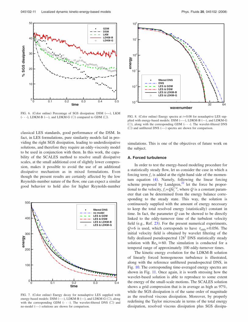
The effectiveness of the SGS modeling is first demon-

strated by making a comparison with the no-model solution.

The latter has been found to be initially underdissipative �see

Fig. 7�, thus confirming the need for the extra dissipation

provided by the SGS model. However, the absence of mod-

eled SGS dissipation results in energy transfer to the small

scales, where the energy is dissipated by viscous stresses.

Owing to the self-adaptive nature of the numerical method,

this process results in increasing the number of resolved

modes that causes the solution in practice to evolve toward

the DNS approach.

FIG. 1. �Color online� Energy decay: �a� LKM �—� and DSM �- - -�; �b�LDKM-B �- - -� and LDKM-G �—�. The reference GDM �–·–� and wavelet-

filtered DNS �� solutions are shown for comparison.


As shown in Fig. 4, the gain in terms of compression

with respect to the no-model solution is clear. The present

grid compression is above 99.5% for all the different pro-

posed models at all time instants, which corresponds to re-

taining about 1% of the 1923 modes used for dealiasing by

the pseudospectral DNS.6

The achieved compression is com-

parable to the reference GDM.7

The fact that different mod-

els show different compression, though using the same rela-

tive wavelet thresholding level, is not surprising because the

adaptive gridding is closely coupled to the flow physics and,

therefore, it is strongly affected by the presence and type of

the SGS stress model forcing.

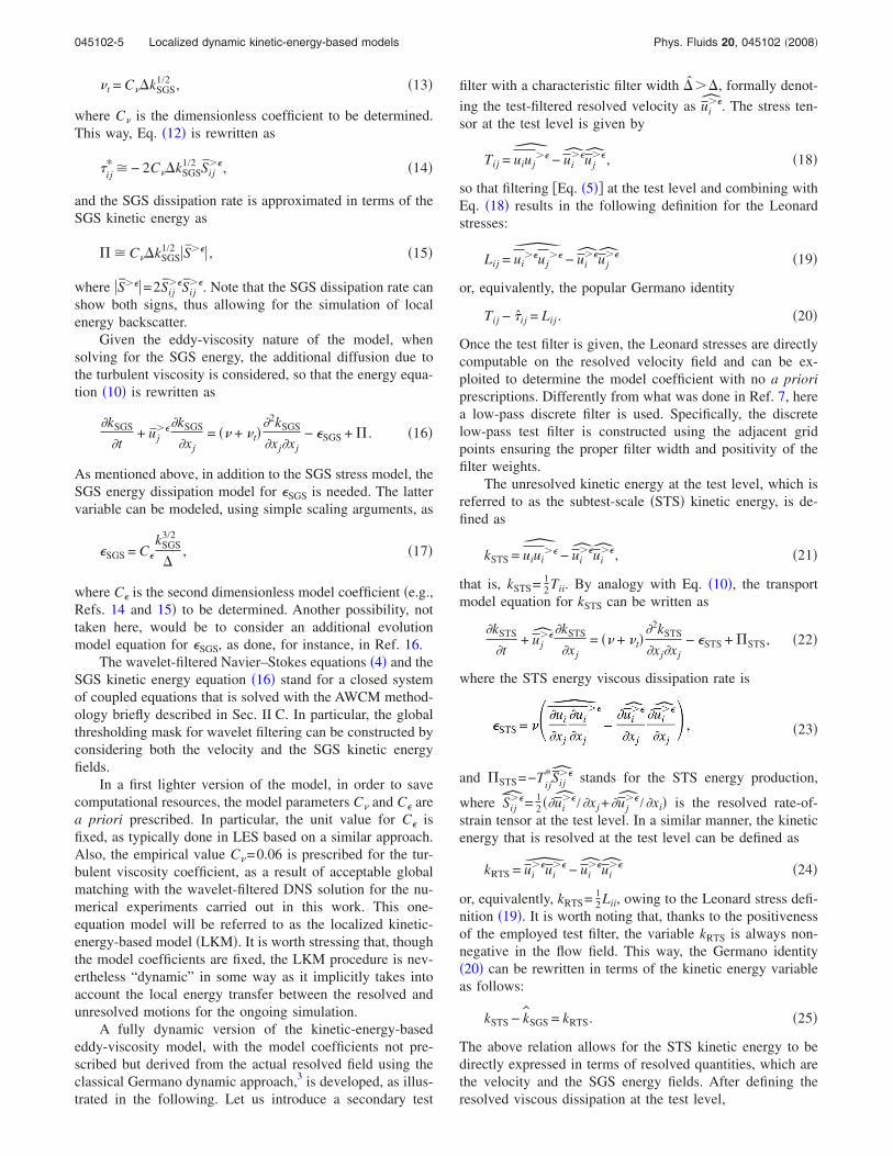
The direct coupling of grid compression with resolved

and SGS dissipation can be clearly seen by examining Figs.

4–6. The decrease of SGS dissipation �in the DSM case�results in the decrease of grid compression and the increase

of resolved energy dissipation. This reinforces the above dis-

cussion about the effectiveness of the model. Also note that,

despite the initial similar compression and similar initial

level of SGS dissipation, the compression for the GDM is

higher. In fact, the nonlocal character of the GDM results in

overdissipation at small scales and fewer wavelet coefficients

on the finest levels, which ultimately results in the earlier

complete removal of the highest level of resolution from the

adaptive computational grid, as clearly seen in Figs. 2 and 3.

In contrast to the global model, the new models are capable

FIG. 2. �Color online� Energy spectra at t=0.08: �a� LKM �–·–� and DSM

�- - -�; �b� LDKM-B �–·–� and LDKM-G �- - -�. The reference GDM �—�and wavelet-filtered DNS �� solutions are shown for comparison, along

with the unfiltered DNS �–··–�.

FIG. 3. �Color online� Energy spectra at t=0.16: �a� LKM �–·–� and DSM

�- - -�; �b� LDKM-B �–·–� and LDKM-G �- - -�. The reference GDM �—�and wavelet-filtered DNS �� solutions are shown for comparison, along

with the unfiltered DNS �–··–�.


of capturing the local structure of the flow rather than pro-

viding only the mean energy dissipation.

We want to emphasize that, differently from classical

LES, the SCALES solution matches the filtered DNS not

only in terms of temporal evolution of the total resolved

energy �or other global quantities� but also in terms of recov-

ering the DNS energy and enstrophy spectra up to the dissi-

pative wavenumber range. This close match is achieved by

using less than 0.5% of the total nonadaptive nodes required

for a DNS calculation with the same wavelet solver. To high-

light the significance of such an agreement, one can compare

the present results �as shown in Figs. 1 and 2� with those

corresponding to 643 finite-difference nonadaptive LES sup-

plied with either the global dynamic Smagorinsky model �as

reported in Ref. 21� or the present energy-based SGS mod-

els. Despite the fact that LES solutions use about three times

the number of modes, they fail to capture the small-scale

features of the flow and the resolved kinetic energy spectrum

is noticeably lower than the filtered DNS one for moderate

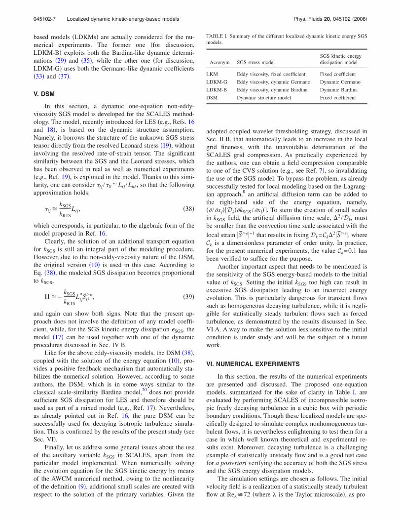
and high wavenumbers. This leads to the underestimation of

the energy content of the flow field so that the LES solutions

appear overdissipative for the first half of the simulation pe-

riod, as illustrated in Figs. 7 and 8, where the energy evolu-

tion and energy spectra for nonadaptive LES supplied with

energy-based models are reported. These differences are

more pronounced for the enstrophy spectra, which are illus-

trated in Fig. 9 �for t=0.08�. This is even more important

since the enstrophy spectra, if properly normalized, coincide

with the viscous dissipation spectra, so that the close agree-

ment provided by wavelet-based adaptive LES ensures

proper spectral distribution of resolved viscous dissipation.

Finally, it is instructive to discuss the “unexpected,” by

FIG. 4. �Color online� Grid compression: �a� DSM �- - -� and LKM �—�; �b�LDKM-B �- - -� and LDKM-G �—�. The no-model �� and GDM �–··–�solutions are shown for comparison.

FIG. 5. �Color online� Energy dissipation: �a� LKM �—� and DSM �–·–�; �b�LDKM-B �—� and LDKM-G �–·–�. The reference GDM �- - -� and wavelet-

filtered DNS �� solutions are shown for comparison.


classical LES standards, good performance of the DSM. In

fact, in LES formulations, pure similarity models fail in pro-

viding the right SGS dissipation, leading to underdissipative

solutions, and therefore they require an eddy-viscosity model

to be used in conjunction with them. In this work, the capa-

bility of the SCALES method to resolve small dissipative

scales, at the small additional cost of slightly lower compres-

sion, makes it possible to avoid the use of an additional

dissipative mechanism as in mixed formulations. Even

though the present results are certainly affected by the low

Reynolds-number nature of the flow, one can expect a similar

good behavior to hold also for higher Reynolds-number

simulations. This is one of the objectives of future work on

the subject.

A. Forced turbulence

In order to test the energy-based modeling procedure for

a statistically steady flow, let us consider the case in which a

forcing term f i is added at the right-hand side of the momen-

tum equation �4�. Namely, following the linear forcing

scheme proposed by Lundgren,22

let the force be propor-

tional to the velocity, f i=Qui��, where Q is a constant param-

eter that can be determined from the energy balance corre-

sponding to the steady state. This way, the solution is

continuously supplied with the amount of energy necessary

to keep the total resolved energy �statistically� constant in

time. In fact, the parameter Q can be showed to be directly

linked to the eddy-turnover time of the turbulent velocity

field �e.g., Ref. 23�. For the present numerical experiments,

Q=6 is used, which corresponds to have eddy=0.056. The

initial velocity field is obtained by wavelet filtering of the

fully dealiased pseudospectral 1283 DNS statistically steady

solution with Re�60. The simulation is conducted for a

temporal range of approximately 100 eddy-turnover times.

The kinetic energy evolution for the LDKM-B solution

of linearly forced homogeneous turbulence is illustrated,

along with the reference unfiltered pseudospectral DNS, in

Fig. 10. The corresponding time-averaged energy spectra are

shown in Fig. 11. Once again, it is worth stressing how the

wavelet-based solution is able to reproduce to some extent

the energy of the small-scale motions. The SCALES solution

shows a grid compression that is in average as high as 97%,

while the SGS dissipation is of the same order of magnitude

as the resolved viscous dissipation. Moreover, by properly

redefining the Taylor microscale in terms of the total energy

dissipation, resolved viscous dissipation plus SGS dissipa-

time

%S

GS

dis

sip

atio

n

0 0.1 0.2 0.3 0.4 0.50

10

20

30

40

50

GDM

DSM

LKM

LDKM-B

LDKM-G

FIG. 6. �Color online� Percentage of SGS dissipation: DSM �–·–�, LKM

�- - -�, LDKM-B �—�, and LDKM-G �� compared to GDM ��.

time

en

erg

y

0 0.1 0.2 0.3 0.40

100

200

300

400

500

filtered DNS

no model

LES & GDM

LES & DSM

LES & LDKM-B

LES & LDKM-G

FIG. 7. �Color online� Energy decay for nonadaptive LES supplied with

energy-based models: DSM �–··–�, LDKM-B �—�, and LDKM-G ��, along

with the corresponding GDM �- - -�. The wavelet-filtered DNS �� and

no-model �–·–� solutions are shown for comparison.

wavenumber

en

erg

y

32 6410

-3

10-2

10-1

100

101

102

filtered DNS

DNS

LES & GDM

LES & DSM

LES & LDKM-B

LES & LDKM-G

FIG. 8. �Color online� Energy spectra at t=0.08 for nonadaptive LES sup-

plied with energy-based models: DSM �–··–�, LDKM-B �—�, and LDKM-G

��, along with the corresponding GDM �- - -�. The wavelet-filtered DNS

�� and unfiltered DNS �–·–� spectra are shown for comparison.


tion, the wavelet-based solution provides the same Reynolds

number as the reference DNS. These results demonstrate the

effectiveness and efficiency of the energy-based SGS model

in the forced case.

Finally, to definitely verify the stabilizing action of the

built-in feedback mechanism associated with the dynamic

energy-based modeling procedure, the following experiment

is conducted: the initial SGS kinetic energy content of the

flow is artificially altered by multiplying the variable

kSGS�x ,0� by a factor of either 102 or 10−2. This way, the

initial SGS energy is either much more or less than the equi-

librium value provided by the wavelet-filtered DNS solution.

Nevertheless, the LDKM procedure is able to provide a flow

evolution that converges after some time toward the unal-

tered stable solution so that the equilibrium levels are re-

stored. This is clearly illustrated by inspection of Fig. 12,

where the evolutions of resolved and SGS energy are re-

ported. This demonstrates that the energy-based method

works in practice: solving a subgrid energy transport equa-

tion properly represents the energy transfer between resolved

and SGS motions, both forward and backscatter.

VII. CONCLUSIONS AND PERSPECTIVES

New localized dynamic models for SCALES that in-

volve an evolution equation for the subgrid kinetic energy

are proposed. One of the main advantages of the present

formulation is that the equilibrium assumption between pro-

FIG. 9. �Color online� Enstrophy spectra at t=0.08: �a� LKM �—�, DSM

�–·–�, and nonadaptive LES supplied with GDM �–··–�; �b� LDKM-B �—�,LDKM-G �–·–�, and nonadaptive LES supplied with LDKM-G �–··–�. The

reference GDM �� and wavelet-filtered DNS �� solutions are shown for

comparison, along with the unfiltered DNS �- - -�.

time

reso

lve

d&

SG

Se

ne

rgy

0 1 2 3 4 5 60

400

800

1200

resolved

SGS

DNS

FIG. 10. �Color online� LDKM-B solution of forced turbulence: resolved

�–·–� and SGS �- - -� energy, along with the reference DNS solution �—�.

wavenumber

en

erg

y

16 32 48 6410

-5

10-4

10-3

10-2

10-1

100

101

102

103

DNS

LDKM-B

FIG. 11. �Color online� LDKM-B solution of forced turbulence: averaged

energy spectrum �- - -� along with the reference DNS �—�.


duction and dissipation of SGS energy is not required as in

the classical Smagorinsky approach. In contrast, the energy

transfer between resolved and residual motions is directly

ensured by solving an additional transport model equation

for the SGS energy. Some known difficulties, associated with

the classical dynamic Germano model, are overcome using

these models. Specifically, scaling SGS in terms of the SGS

kinetic energy provides a feedback mechanism that makes

the numerical simulation stable regardless of whether an

eddy-viscosity or non-eddy-viscosity assumption is made.

This way, no averaging procedure is needed in practice and

the models stay fully localized in space.

The present study demonstrates how the proposed one-

equation models work for statistically unsteady flows shed-

ding light on the possible use of the SCALES methodology

for complex flow simulation. The energy-based models are

assessed in terms of both accuracy and efficiency. In fact, the

results match the filtered DNS data at different times with a

grid compression comparable if not higher than that achieved

with the GDM.

Furthermore, for forced turbulence simulation, it is dem-

onstrated that the dynamic energy-based modeling procedure

obtains a stable solution with the level of energy and the

energy spectrum comparable to those ones of the correspond-

ing reference spectral DNS. It is verified that the model ac-

tually controls backscatter-induced instabilities over long

time integration.

As to future work, once a more cost effective implemen-

tation is developed, the method will allow for the simulation

of complex nonhomogeneous and statistically unsteady

flows. For instance, transitional as well as intermittent turbu-

lent flows of engineering interest will be simulated without

the need of introducing additional ad hoc assumptions for

calibrating the SGS model parameters. Also, by explicitly

taking care of the residual kinetic energy, the use of one-

equation models will allow the numerical simulation of high

Reynolds-number flows with reasonable computational

grids, which is one of the primary objectives of the SCALES

development.

Finally, it is worth stressing that, with the introduction of

the SCALES methodology, the incompleteness of classical

LES implementations has been partly removed. However, the

approach maintains a certain subjectivity due to the prescrip-

tion of the relative thresholding level for wavelet filtering. A

fully adaptive SCALES formulation in which this threshold

automatically varies in time based on the instantaneous flow

conditions is under study. For instance, as suggested in Ref.

4, the ratio between SGS and resolved kinetic energy can be

assumed as a measure of the actual turbulence resolution.

Thus, by explicitly involving an evolution equation for the

residual kinetic energy, the wavelet thresholding level could

be automatically varied in order to maintain the desired level

of turbulence resolution for the ongoing simulation.

ACKNOWLEDGMENTS

This work was supported by the Department of Energy

�DOE� under Grant No. DE-FG02-05ER25667, the National

Science Foundation �NSF� under Grant Nos. EAR-0327269

and ACI-0242457, and the National Aeronautics and Space

Administration �NASA� under Grant No. NAG-1-02116. In

addition, G.D.S. was partially supported by a grant from Re-

gione Campania �LR 28/5/02 n.5�.

1J. S. Smagorinsky, “General circulation experiments with the primitive

equations,” Mon. Weather Rev. 91, 99 �1963�.2J. W. Deardorff, “Three-dimensional numerical study of turbulence in an

entraining mixed layer,” Boundary-Layer Meteorol. 7, 199 �1974�.3M. Germano, U. Piomelli, P. Moin, and W. Cabot, “A dynamic subgrid-

scale eddy-viscosity model,” Phys. Fluids A 3, 1760 �1991�.4S. B. Pope, “Ten questions concerning the large-eddy simulation of turbu-

lent flows,” New J. Phys. 6, 1 �2004�.5D. E. Goldstein and O. V. Vasilyev, “Stochastic coherent adaptive large

eddy simulation method,” Phys. Fluids 16, 2497 �2004�.

FIG. 12. �Color online� Energy evolutions for LDKM-B solution of forced

turbulence with initial SGS energy altered by a factor of either 102 �–·–� or

10−2 �- - -�: �a� resolved and �b� SGS energy are reported along with the

unaltered solution �—�.


6G. De Stefano, D. E. Goldstein, and O. V. Vasilyev, “On the role of

sub-grid scale coherent modes in large eddy simulation,” J. Fluid Mech.

525, 263 �2005�.7D. E. Goldstein, O. V. Vasilyev, and N. K.-R. Kevlahan, “CVS and

SCALES simulation of 3D isotropic turbulence,” J. Turbul. 6, 1 �2006�.8O. V. Vasilyev, G. De Stefano, D. E. Goldstein, and N. K.-R. Kevlahan,

“Lagrangian dynamic SGS model for SCALES of isotropic turbulence,” J.

Turbul. 9, 1 �2008�.9M. Farge, K. Schneider, and N. K.-R. Kevlahan, “Non-Gaussianity and

coherent vortex simulation for two-dimensional turbulence using an adap-

tive orthogonal wavelet basis,” Phys. Fluids 11, 2187 �1999�.10

M. Farge, K. Schneider, G. Pellegrino, A. A. Wray, and R. S. Rogallo,

“Coherent vortex extraction in three-dimensional homogeneous turbu-

lence: Comparison between CVS-wavelet and POD-Fourier decomposi-

tions,” Phys. Fluids 15, 2886 �2003�.11

O. V. Vasilyev, “Solving multi-dimensional evolution problems with lo-

calized structures using second generation wavelets,” Int. J. Comput. Fluid

Dyn. 17, 151 �2003�, special issue on high-resolution methods in compu-

tational fluid dynamics.12

N. K.-R. Kevlahan and O. V. Vasilyev, “An adaptive wavelet collocation

method for fluid-structure interaction at high Reynolds numbers,” SIAM J.

Sci. Comput. �USA� 26, 1894 �2005�.13

O. V. Vasilyev and N. K.-R. Kevlahan, “An adaptive multilevel wavelet

collocation method for elliptic problems,” J. Comput. Phys. 206, 412

�2005�.14

S. Ghosal, T. S. Lund, P. Moin, and K. Akselvoll, “A dynamic localization

model for large-eddy simulation of turbulent flows,” J. Fluid Mech. 286,

229 �1995�.15

U. Schumann, “Subgrid scale model for finite difference simulations of

turbulent flows in plane channels and annuli,” J. Comput. Phys. 18, 376

�1975�.16

E. Pomraning and C. J. Rutland, “Dynamic one-equation nonviscosity

large-eddy simulation model,” AIAA J. 40, 689 �2002�.17

W.-W. Kim and S. Menon, “An unsteady incompressible Navier–Stokes

solver for large eddy simulation of turbulent flows,” Int. J. Numer. Meth-

ods Fluids 31, 983 �1999�.18

S. G. Chumakov and C. J. Rutland, “Dynamic structure subgrid-scale

models for large eddy simulation,” Int. J. Numer. Methods Fluids 47, 911

�2005�.19

S. Liu, C. Meneveau, and J. Katz, “On the properties of similarity subgrid-

scale models as deduced from measurements in a turbulent jet,” J. Fluid

Mech. 262, 83 �1994�.20

J. Bardina, J. H. Ferziger, and W. C. Reynolds, “Improved turbulence

models based on large eddy simulation of homogeneous incompressible

turbulence,” Thermosciences Division, Mechanical Engineering Depart-

ment, Stanford University, Report No. TF-19, 1983.21

O. V. Vasilyev, D. E. Goldstein, G. De Stefano, D. Bodony, D. You, and L.

Shunn, “Assessment of local dynamic subgrid-scale models for stochastic

coherent adaptive large eddy simulation,” in Proceedings of the 2006 Sum-

mer Program �Center for Turbulence Research, NASA Ames/Stanford

University, Stanford, CA, 2006�, pp. 139–150.22

T. S. Lundgren, “Linearly forced isotropic turbulence,” Annual Research

Briefs �Center for Turbulence Research, NASA Ames/Stanford University,

Stanford, CA, 2003�, pp. 461–473.23

C. Rosales and C. Meneveau, “Linear forcing in numerical simulations of

isotropic turbulence: Physical space implementations and convergence

properties,” Phys. Fluids 17, 095106 �2005�.


Localized dynamic kinetic-energy-based models for stochastic coherent adaptive large eddy simulation

Documents

Transcript of Localized dynamic kinetic-energy-based models for stochastic coherent adaptive large eddy simulation