Localization Control to Locate Mobile Sensors

Localization Control to Locate Mobile Sensors

Buddhadeb Sau1, Srabani Mukhopadhyaya2, and Krishnendu Mukhopadhyaya3

1 Dept. of Maths., Jadavpur University, Kolkata, [email protected]

2 BIT Mesra, Kolkata, [email protected]

3 ACMU, Indian Statistical Institute, Kolkata, [email protected]

Abstract. Localization is an important issue for Wireless Sensor Net-works in a wireless sensor network. A mobile sensor may change its posi-tion rapidly and thus require localization calls frequently. It is importantto control the number of localization calls, as it is rather expensive. Theexisting schemes for reducing the frequency of localization calls for mo-bile sensors uses the technique of extrapolation which involves simplearithmetic calculations. We propose a technique to control the localiza-tion that gives much better result. The proposed method involves verylow arithmetic computation overheads. We find analytical expressionsfor the estimated error if the rate of localizations is specified. Simulationstudies are carried out to compare the performances of the proposedmethod with the methods proposed by Tilak et al.

Keywords: Wireless sensor network, localization, mobility, localizationcontrol, target tracking.

1 Introduction

A micro-sensor (or simply a sensor) is a small sized and low powered electronicdevice with limited computational and communication capabilities. A WirelessSensor Network (WSN) is a network containing some ten to millions of suchmicro-sensors. If the sensors are deployed randomly, or the sensors move aboutafter deployment, finding the locations of sensors (localization) is an importantissue in WSN. Localization requires communication of several necessary informa-tion between sensors over the network and a lot of computations. All these comesat the cost of high energy consumption. So far, research have mainly been fo-cused on finding efficient localization techniques in static sensor networks (wherethe sensor nodes do not change their positions after deployment) [2,3,4].

Dynamic sensor networks have immense applications giving assistance to mo-bile soldiers in a battle field, health monitoring, in wild-life tracking [6], etc.When a sensor moves, it needs to find its position frequently. Using Global Po-sitioning System (GPS) may not be appropriate due to its low accuracy, highenergy consumption, cost and size. An optimized localization technique of staticsensor network is used to find the current position of a mobile sensor. A fast

S. Madria et al. (Eds.): ICDCIT 2006, LNCS 4317, pp. 81–88, 2006.c© Springer-Verlag Berlin Heidelberg 2006

82 B. Sau, S. Mukhopadhyaya, and K. Mukhopadhyaya

mobile sensor may require frequent localizations, draining the valuable energyquickly.

Thurn et al [5] proposed probabilistic techniques using Monte Carlo localiza-tion (MCL) to estimate the location of mobile robots with probabilistic knowl-edge on movement over predefined map. They used a small number of seed nodes(nodes with known position), as beacons. These nodes have some extra hard-ware. Hu et al [9] introduced the sequential MCL to exploit the mobility withoutextra hardware. WSNs generally remain embedded in an unmapped terrain andsensors have no control on their mobility. In [8], the objective is to reduce thenumber of localization calls. The positions of a sensor at different time instantare estimated from the history of the path of the sensor.

Tilak et al [7] proposed a number of techniques for tracking mobile sensorsbased on dead reckoning. The objective again is to control the number of costly lo-calization operations. Among these techniques, the best performance is achievedby Mobility Aware Dead Reckoning Driven (MADRD). MADRD estimates theposition of a sensor, in stead of localizing the sensor every time it moves. Errorin the estimated position grows with time. Every time localization is called, theerror in the estimated position is calculated. Depending on the value of this errorthe time for the next localization is fixed. Fast mobile sensors t rigger localizationwith higher frequency for a given level of accuracy in position estimation.

In this paper, a method is proposed to estimate the positions of a mobilesensor, in stead of localizing the sensor. It gives higher accuracy for a particularenergy cost and vice versa. The position of a sensor is required only when thesensor has some data is to be sent. The information of an inactive sensor isceased to be communicated. Most calculations are carried out at the base stationto reduce arithmetic complexity of sensors.

Section 2 describes the problem for tracking mobile sensor. In Section 3 wedescribe different algorithms for tracking mobile sensors. Section 4 deals withthe analysis of the algorithm and different advantages. In Section 5 simulationresults are presented. Finally, we present our conclusion in Section 6.

2 Problem Statement and Performance Measures

The position of a sensor is determined by a standard localization method. Weassume that the location determined by this localization represents the actualposition of the sensor at that moment. The sensors are completely unaware ofthe mobility pattern. Therefore, the actual position of a sensor S any time tis unknown. The position may be estimated or found by localization call. Theabsolute error in location estimation may be calculated as:

errorabs =√

(xt − xt)2 + (yt − yt)2

where (xt, yt) and (xt, yt) denote the actual and estimated positions at time trespectively. Frequent call of localization consumes enormous energy. To devisean algorithm optimizing both accuracy and energy dissipation simultaneously isvery difficult. An efficient, robust and energy aware protocol is required to decide

Localization Control to Locate Mobile Sensors 83

whether the location of the sensor would be estimated with a desired level ofaccuracy or found by localization with an acceptable level of energy cost.

3 Localization Protocol for Tracking Mobile Sensors

A mobile sensor changes its position with time. A simple strategy for findingits position is the use of standard localization methods at any time. But if theposition of the sensor is required frequently, this method is very costly. Tilaket. al tried to reduce the frequency of localizations for finding the position ofsensors. They proposed techniques: Static Fixed Rate (SFR), Dynamic VelocityMonotonic (DVM) and Mobility Aware Dead Reckoning Driven (MADRD).

SFR calls a classical localization operation periodically with a fixed time in-terval. To respond a query from the base station, a sensor sends its positionobtained from the last localization. When a sensor remains still or moves fast,in both cases, the reported position suffers a large error. In DVM, localization iscalled adaptively with the mobility of the sensors. The time interval for the nextcall for localization is calculated as the time required to traverse the thresholddistance (a distance, traversed by the sensor, location estimation assumed tobe error prone) with the velocity of the sensor between last two points in thesequence of localization calls. In case of high mobility, a sensor calls localizationfrequently. If a sensor suddenly moves with very high speed from rest, error inthe estimated location becomes very high. In MADRD, the velocity is calculatedfrom the information obtained from last two localized points. The predictor esti-mates the position with this velocity and communicates to the query sender. Atthe localization point, the localized position is reported to the query sender andthe distance error is calculated as the distance between the predicted positionand reported position. If the error in position estimation exceeds threshold error(application dependent), the predictor appears to be erroneous and localizationneeds to be triggered more frequently. The calculation of error is necessary everytime a localization called. Also, a sensor with high speed calls localizations fre-quently. We propose a new method, Mobility Aware Interpolation (MAINT), toestimate the current position with better tradeoff between the energy consump-tion and accuracy. The proposed method, MAINT, uses interpolation which givesbetter estimation in most cases.

3.1 Mobility Aware Interpolation (MAINT)

In some applications of dynamic sensor networks, the base station may need thelocations of individual sensors at different times. The location may be requiredto be attached to the data gathered by the sensors in response to a query.However, the data may not be required immediately. In such cases, the number oflocalization calls may be reduced by delaying the response. The sensor holds thequeries requiring the the location, into a list, queryPoints and sends the eventto the base station padding the time of occurrence. At the following localizationpoint, the sensor sends these two localized positions to each of the query senders


in the time interval between these two localization points which are alreadyin the list. The base station estimates the positions with more accuracy byinterpolation with this information. The time interval of localization calls isas simple as in SFR. It eliminates all the arithmetic overheads as opposed toMADRD and the error prone nature in sudden change of speeds. Unnecessarycalls of localizations for slow sensors may be avoided. To reduce the energydissipation, the localization method may be called with higher time interval.The localization may be called immediately after receiving the query for realtime applications or some special purpose. Each sensor runs a process with thealgorithm described as follows :

Algorithm 1 (MAINT:)

Step-1: Let (x1, y1) denotes the last localization point occured at time t1.And let queryPoints = φ .

Step-2: While(a query received from a sensor S at time t > t1)Append S to queryPoints, if S /∈ queryPoints.If (response to the query is immediate) or (t ≥ t1 + T ) then

/* Call an optimized localization method */Let (x, y) be the location obtained from the method;While (queryPoints ! = φ) do

Extract a query sender, say S′, from queryPoints;Send t1, t, (x1, y1) and (x, y) to S′

End /* end of while */Set t1 = t and (x1, y1) = (x, y).

endifEnd while

After receiving a message from a sensor, the base station waits until it getslocation information of the sender, S. If the processing of the message is immedi-ate, the base station may send location query to the node S. However, the basestation extracts localization points from the response obtained from S againstthe location query and estimates the location of S as follows:

Let (x1, y1) and (x2, y2) be the localized positions of the sensor s at t1 and t2.if (t′ ∈ [t1, t2])

Calculate the velocity vector asx = (x2 − x1)/(t2 − t1); y = (y2 − y1)/(t2 − t1);

Estimate the position of s at time t′ ∈ [t1, t2] asx′ = x1 + x(t′ − t1); y′ = y1 + y(t′ − t1);

where t′ be a time at which the position of S is required by the base station.

4 Energy and Error Analysis

Energy consumption due to a localization call is much higher than other factorsin dynamic localization. In the error analysis, we consider energy dissipation


only by localization calls. We assume, the energy consumption is proportionalto the number of localization calls. Therefore, we measure energy in terms ofnumber of localization calls. Assume that MAINT occurs with a time intervalT . The error evaluation is performed uniformly over the time interval [0, T ].

4.1 Motion Analysis with Random Waypoint Model

The Random WayPoint (RWP) is a commonly used synthetic model for mobil-ity. We carried out the simulation study as well as analysis with RWP mobil-ity model. In Figure 1 the sensor starts from S0(x0, y0) and reaches the pointST (xT , yT ) at time T . The sequence of the waypoints attended by the sensor inthe time interval [0, T ] is S0, S1, · · · , Sn, ST .

MADRD

MAINT

ACTUAL

S0

S1

S2

S3

Si−1

Si

Sn

ST

S′T

×P ′(x′, y′)

×P (x, y)

×P ′′(x′′ , y

′′)

Fig. 1. Figure showing localization calls at two points and the position estimates forthe intermediate points by MADRD and MAINT

At any waypoint Si−1(xi−1, yi−1) next waypoint Si(xi, yi) is selected ran-domly with independent and identical uniform distribution over the rectangulararea R = {(x, y) : 0 ≤ x ≤ X, 0 ≤ y ≤ Y }. We assume that the occurrenceof waypoints follows the Poisson Process. Let ti be the duration of the intervalfollowed by the waypoint Si−1(xi−1, yi−1) and (ui, vi) be the velocity compo-nents during this period. Therefore, the inter arrival times ti : 1 ≤ i ≤ n ofthe waypoints are independent and identically distributed and follow exponen-tial distribution with parameter λ. The sum Ti = t1 + t2 + · · · + ti is a randomvariable and follows gamma distribution with parameters λ and i. The numberof waypoints n such that Tn ≤ T and Tn+1 > T , follows the Poisson distribu-tion with mean λT . Let P (x, y) be the actual position of the sensor at time t,0 ≤ ti−1 ≤ t ≤ ti ≤ T . Then

x = xi−1 + (t − Ti−1)ui, y = yi−1 + (t − Ti−1)vi

for i = 1, 2, . . . , n and T0 = 0.


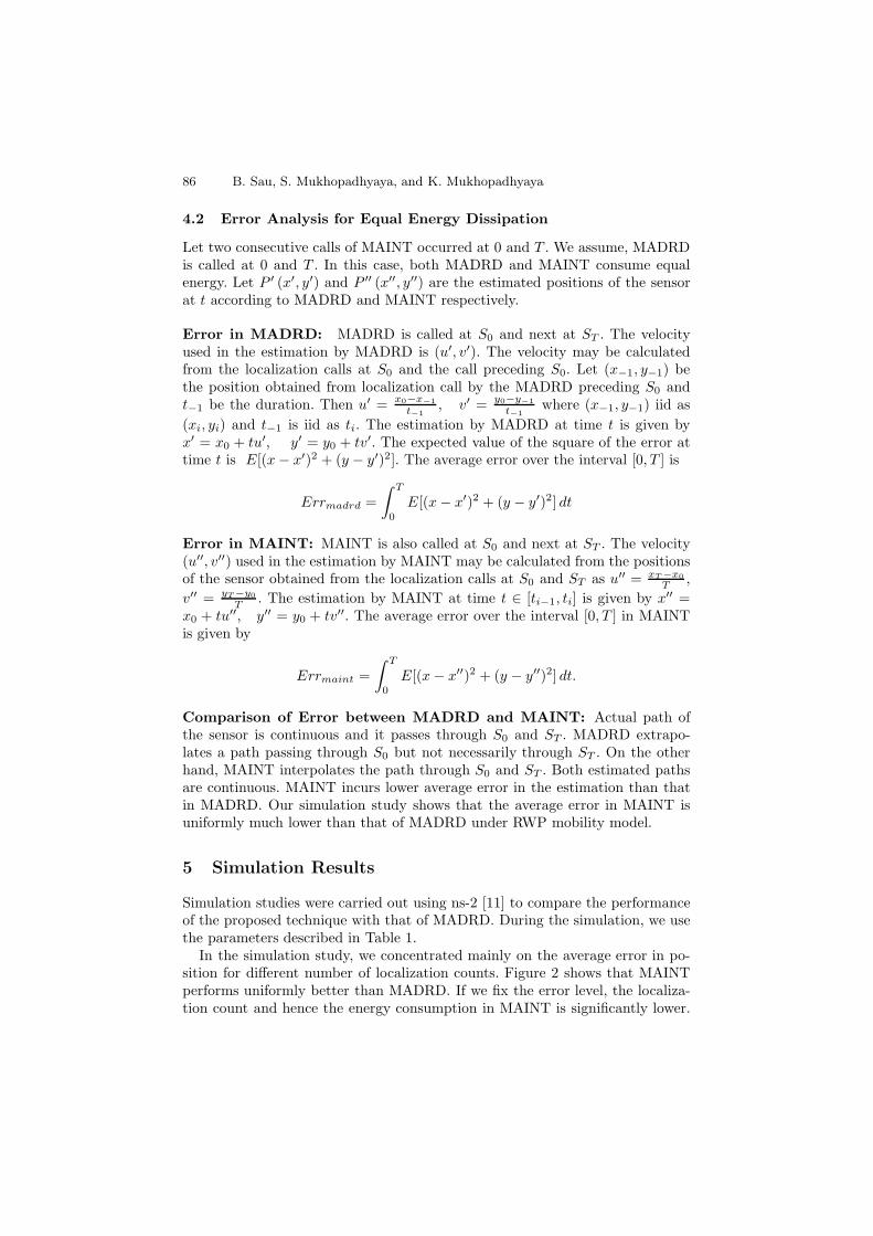
4.2 Error Analysis for Equal Energy Dissipation

Let two consecutive calls of MAINT occurred at 0 and T . We assume, MADRDis called at 0 and T . In this case, both MADRD and MAINT consume equalenergy. Let P ′ (x′, y′) and P ′′ (x′′, y′′) are the estimated positions of the sensorat t according to MADRD and MAINT respectively.

Error in MADRD: MADRD is called at S0 and next at ST . The velocityused in the estimation by MADRD is (u′, v′). The velocity may be calculatedfrom the localization calls at S0 and the call preceding S0. Let (x−1, y−1) bethe position obtained from localization call by the MADRD preceding S0 andt−1 be the duration. Then u′ = x0−x−1

t−1, v′ = y0−y−1

t−1where (x−1, y−1) iid as

(xi, yi) and t−1 is iid as ti. The estimation by MADRD at time t is given byx′ = x0 + tu′, y′ = y0 + tv′. The expected value of the square of the error attime t is E[(x − x′)2 + (y − y′)2]. The average error over the interval [0, T ] is

Errmadrd =∫ T

0E[(x − x′)2 + (y − y′)2] dt

Error in MAINT: MAINT is also called at S0 and next at ST . The velocity(u′′, v′′) used in the estimation by MAINT may be calculated from the positionsof the sensor obtained from the localization calls at S0 and ST as u′′ = xT −x0

T ,v′′ = yT −y0

T . The estimation by MAINT at time t ∈ [ti−1, ti] is given by x′′ =x0 + tu′′, y′′ = y0 + tv′′. The average error over the interval [0, T ] in MAINTis given by

Errmaint =∫ T

0E[(x − x′′)2 + (y − y′′)2] dt.

Comparison of Error between MADRD and MAINT: Actual path ofthe sensor is continuous and it passes through S0 and ST . MADRD extrapo-lates a path passing through S0 but not necessarily through ST . On the otherhand, MAINT interpolates the path through S0 and ST . Both estimated pathsare continuous. MAINT incurs lower average error in the estimation than thatin MADRD. Our simulation study shows that the average error in MAINT isuniformly much lower than that of MADRD under RWP mobility model.

5 Simulation Results

Simulation studies were carried out using ns-2 [11] to compare the performanceof the proposed technique with that of MADRD. During the simulation, we usethe parameters described in Table 1.

In the simulation study, we concentrated mainly on the average error in po-sition for different number of localization counts. Figure 2 shows that MAINTperforms uniformly better than MADRD. If we fix the error level, the localiza-tion count and hence the energy consumption in MAINT is significantly lower.


Table 1. Relevant parameters used in simulation

Simulation area 300 × 300 m2 Transmit power 0.660 WTransmission range 10m Receive power 0.395 WInitial Energy 10000 J Idle power 0.035 WMAC protocol 802.11 Number of mobile nodes 24

Number of beacon nodes 36

Also, for comparable numbers of localization count, MAINT has much lower av-erage error. MAINT estimates the position of a sensor with less error and evenconsuming less energy.

0

2

4

6

8

10

12

14

16

0 10 20 30 40 50 60 70 80 90 100

Err

or in

pos

ition

Localization Count

MAINTMADRD

Fig. 2. Figure showing average error and localization counts for MADRD and theproposed technique

MAINT locates a mobile sensor with nearly exact position of the sensor con-suming approximately half energy than that of MADRD. MAINT requires highermemory to hold the history of location queries. To reduce the memory require-ment, we can hold limited number of most recent query points.

6 Conclusion

The technique, proposed in this paper, uses estimates of the location of a mobilesensor to save on the energy used up in frequent calls for localization. In MADRD,the velocity of a sensor is calculated using the time and location of the last twopoints of localization. This velocity is later used to extrapolate the position of thesensor at a later time. In comparison, MAINT uses interpolation. The velocity is


similarly calculated but not from the last two points, rather from the last localiza-tion point and the next localization point. So the position can be estimated onlyafter the next localization takes place. Simulation studies show that MAINT es-timates the position of the sensor with much lower error than that of MADRD.Simulation study in this paper was carried out using RWP mobility model. How-ever, analysis of the proposed technique shows that MAINT estimates the pathwith lower error for any other mobility model. Simulation works using other mo-bility models like the Gaussian movement model, Brownian motion model etc.,are in progress.

References

1. Akyldiz, I.F., Su, W., Sankarasubramaniam, Y., Cayh’ci, E.: Wh’eless Sensor Net-works: A Survey. Computer Networks, Vol. 38, No. 4. March (2002) 393–422

2. Bulusu, N., Heidemann, J., Estrin, D.: GPS-less Low Cost Outdoor LocalizationFor Very Small Devices. IEEE Personal Communications Magazine, Vol. 7, No. 5.October (2000) 28–34

3. Meguerdichian, S., Koushanfar, F., Qu, G., Potkonjak, M.: Exposure In WirelessAd-Hoc Sensor Networks. Proc. 7th Int. Conf. on Mobile Computing and Network-ing (MobiCom’01). Rome, Italy July (2001) 139–150

4. Raghunathan, V., Schurgers, C., Park, S., Srivastava, M.B.: Energy-aware wirelessmicrosensor networks. IEEE Signal Processing Magazine, vol. 19, No. 2. IEEEMarch (2002) 40–50

5. Thrun, S., Fox, D., Burgard, W., Dellaert, F.: Robust Monte Carlo Localizationfor Mobile Robots. Artificial Intelligence (2001)

6. Juang, P., Oki, H., Wang, Y., Martonosi, M., Peh, L.S., Rubenstein, D.: Energy-efficient computing for wildlife tracking: design tradeoffs and early experienceswith zebranet. Proc. of 10th Int. Conf. on Architectural Support for ProgrammingLanguages and Operating Systems (ASPLOS-X). ACM Press, (2002) 96–107

7. Tilak, S., Kolar, V., Abu-Ghazaleh, N.B., Kang, K.D.: Dynamic Localization Con-trol for Mobile Sensor Networks. IEEE Int. Workshop on Strategies for EnergyEfficiency in Ad-Hoc and Sensor Networks(IEEEIWSEEASN-2005).

8. Bergamo, P., Mazzini, G.: Localization in Sensor Networks with Fading the Mo-bility. IEEE PIMRC. September (2002)

9. Hu, L., Evans, D.: Localization in Mobile Sensor Networks. MobiCom’04, Sept.26.-Oct.,1 (2004)

10. Bettstetter, C., Wagner, C.: The spatial node distribution of the random waypointmobility model. In Proceedings of German Workshop on Mobile Ad Hoc networks(WMAN), Ulm, Germany, March (2002)

11. Network Simulator : http://isi.edu/nsnam/ns

Localization Control to Locate Mobile Sensors

Documents

Transcript of Localization Control to Locate Mobile Sensors