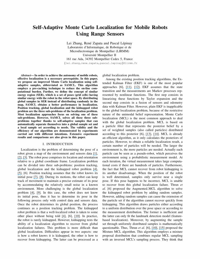
Self-Adaptive Monte Carlo Localization for Mobile RobotsUsing Range Sensors

Lei Zhang, Rene Zapata and Pascal LepinayLaboratoire d’Informatique, de Robotique et de

Microelectronique de Montpellier (LIRMM)Universite Montpellier II

161 rue Ada, 34392 Montpellier Cedex 5, France{lei.zhang,rene.zapata,pascal.lepinay}@lirmm.fr

Abstract— In order to achieve the autonomy of mobile robots,effective localization is a necessary prerequisite. In this paper,we propose an improved Monte Carlo localization using self-adaptive samples, abbreviated as SAMCL. This algorithmemploys a pre-caching technique to reduce the on-line com-putational burden. Further, we define the concept of similarenergy region (SER), which is a set of poses (grid cells) havingsimilar energy with the robot in the robot space. By distributingglobal samples in SER instead of distributing randomly in themap, SAMCL obtains a better performance in localization.Position tracking, global localization and the kidnapped robotproblem are the three sub-problems of the localization problem.Most localization approaches focus on solving one of thesesub-problems. However, SAMCL solves all these three sub-problems together thanks to self-adaptive samples that canautomatically separate themselves into a global sample set anda local sample set according to needs. The validity and theefficiency of our algorithm are demonstrated by experimentscarried out with different intentions. Extensive experimentresults and comparisons are also given in this paper.

I. INTRODUCTION

Localization is the problem of determining the pose of arobot given a map of the environment and sensors data [1],[2], [3]. The robot pose comprises its location and orientationrelative to a global coordinate frame. Localization problemcan be divided into three sub-problems: position tracking,global localization and the kidnapped robot problem [4],[5], [6]. Position tracking assumes that the robot knows itsinitial pose [7], [8]. During its motions, the robot can keeptrack of movement to maintain a precise estimate of its poseby accommodating the relatively small noise in a knownenvironment. More challenging is the global localizationproblem [4], [9]. In this case, the robot does not knowits initial pose, thus it has to determine its pose in thefollowing process only with control data and sensors data.Once the robot determines its global position, the processcontinues as a position tracking problem. The kidnappedrobot problem is that a well-localized robot is taken to someother place without being told [4], [6], [10]. In practice,the robot is rarely kidnapped. However, kidnapping tests theability of a localization algorithm to recover from globallocalization failures. This problem is more difficult thanglobal localization. Difficulties appear in two aspects: oneis how a robot knows it is kidnapped, the other is how torecover from kidnapping. The latter can be processed as a

global localization problem.Among the existing position tracking algorithms, the Ex-

tended Kalman Filter (EKF) is one of the most popularapproaches [6], [11], [12]. EKF assumes that the statetransition and the measurements are Markov processes rep-resented by nonlinear functions. The first step consists inlinearizing these functions by Taylor expansion and thesecond step consists in a fusion of sensors and odometrydata with Kalman Filter. However, plain EKF is inapplicableto the global localization problem, because of the restrictivenature of the unimodal belief representation. Monte Carlolocalization (MCL) is the most common approach to dealwith the global localization problem. MCL is based ona particle filter that represents the posterior belief by aset of weighted samples (also called particles) distributedaccording to this posterior [6], [13], [14]. MCL is alreadyan efficient algorithm, as it only calculates the posteriors ofparticles. However, to obtain a reliable localization result, acertain number of particles will be needed. The larger theenvironment is, the more particles are needed. Actually eachparticle can be seen as a pseudo-robot, which perceives theenvironment using a probabilistic measurement model. Ateach iteration, the virtual measurement takes large computa-tional costs if there are hundreds of particles. Furthermore,the fact that MCL cannot recover from robot kidnapping isits another disadvantage. When the position of the robotis well determined, samples only survive near a singlepose. If this pose happens to be incorrect, MCL is unableto recover from this global localization failure. Thrun etal. [6] proposed the Augmented MCL algorithm to solvethe kidnapped robot problem by adding random samples.However, adding random samples can cause the extension ofthe particle set if the algorithm cannot recover quickly fromkidnapping. This algorithm draws particles either accordingto a uniform distribution over the pose space or according tothe measurement distribution. The former is inefficient andthe latter can only fit the landmark detection model (feature-based localization). Moreover, by augmenting the sampleset through uniformly distributed samples is mathematicallyquestionable. Thus, Thrun et al. [6], [10], [15] proposed theMixture MCL algorithm. This algorithm employs a mixtureproposal distribution that combines regular MCL samplingwith an inversed MCL’s sampling process. They think that

the key disadvantage of Mixture MCL is a requirement fora sensor model that permits fast sampling of poses. Toovercome this difficulty, they use sufficient statistics anddensity trees to learn a sampling model from data.

In this paper, we propose an improved Monte Carlo lo-calization with self-adaptive samples (SAMCL) to solve thelocalization problem. This algorithm employs a pre-cachingtechnique to reduce the on-line computational burden ofMCL. Thrun et al. [6] use this technique to reduce costsof computing for beam-based models in the ray castingoperation. Our pre-caching technique decomposes the statespace into two types of grids. The first one is a three-dimensional grid that includes the planar coordinates andthe orientation of the robot. This grid, denoted as G3D, isused to reduce the on-line computational burden of MCL.The other grid is a two dimensional energy grid. We defineenergy as the total information of measurements (the moreinformation, the higher energy). The energy grid, denoted asGE , is used to calculate the Similar Energy Region (SER)which is a subset of GE . Its elements are these grid cellswhose energy is similar to robot’s energy. SER providesa priori information of robot’s position, thus, sampling inSER is more efficient than sampling randomly in the wholemap. Finally, SAMCL can solve position tracking, globallocalization and the kidnapped robot problem together thanksto self-adaptive samples. Self-adaptive samples in this paperare different from the KLD-Sampling algorithm proposedin [6], [16]. The KLD-Sampling algorithm employs thesample set that has an adaptive size to increase the efficiencyof particle filters. Our self-adaptive sample set has a fixedsize, thus it does not lead to the extension of the particle set.This sample set can automatically divide itself into a globalsample set and a local sample set according to differentsituations, such as when the robot is kidnapped or fails tolocalize globally. Local samples are used to track the robot’spose, while global samples are distributed in SER and usedto find the new position of the robot.

The rest of this paper is organized as follows. In sectionII, we briefly review Monte Carlo localization. In sectionIII, we introduce the SAMCL algorithm. Experiment resultsare presented in section IV and finally some conclusions aregiven in section V.

II. MONTE CARLO LOCALIZATION

In the probabilistic framework, the localization problemis described as estimating a posterior belief of the robot’spose at present moment conditioned on the whole history ofavailable data. For mobile robots, the available data are oftwo types: perceptual data and odometry data [6].

bel(xt) = p (xt |z0:t, u1:t ) (1)

Where xt is robot’s pose at time t, which is composedby its two-dimensional planar coordinates and its orienta-tion. The belief function bel(xt) represents the density ofprobability of the pose xt. The term z0:t represents all theexteroceptive measurements from time τ = 0 to τ = t andu1:t represents control data from time τ = 1 to τ = t.

Equation (1) is transformed by Bayes rule, the Markovassumption and the law of total probability, to obtain thefinal recursive equation:

bel(xt) = ηp (zt |xt )∫p (xt |xt−1, ut )bel(xt−1)dxt−1

(2)where η is a normalization constant that ensures bel(xt) tosum up to one. The probability p (xt |xt−1, ut ) is called theprediction model or the motion model, which denotes thetransition of robot state. The probability p (zt |xt ) is thecorrection model or the sensor model, which incorporatessensors information to update robot state.

Different localization approaches represent the posteriorbel(xt) in different ways. MCL represents this posteriorbelief by a set of N weighted particles distributed accordingto this posterior [6], [10]:

bel(xt) ∝{⟨x

[n]t , ω

[n]t

⟩}n=1,···,N

(3)

here x[n]t is a particle that represents a hypothesized pose

of robot at time t. The non-negative numerical parameterω

[n]t is the importance factor which gives a weight to each

particle. The initial belief bel(x0) may be represented byparticles drawn according to a uniform distribution over thestate space if the initial pose of the robot is unknown, or byparticles drawn from a Gaussian distribution centered on thecorrect pose if the initial pose is known approximately.

III. THE SAMCL ALGORITHM

The SAMCL algorithm can solve efficiently all the threesub-problems of localization together. The whole processis illustrated in Fig. 1. SAMCL is implemented in threesteps: (1) Pre-caching the map, (2) Calculating SER, (3)Localization. The first step is executed off line, the othertwo steps are run on line.

Fig. 1. The process of the SAMCL algorithm.

A. Pre-caching the Map

In the localization problem, the map is supposed to beknown by the robot. Hence, a main idea is to decompose thegiven map into grid and to pre-compute measurements foreach grid cell. Our pre-caching technique decomposes thestate space into two types of grids.

Three-dimensional grid (G3D). It includes planar coor-dinates and the orientation. Each grid cell is seen as apseudo-robot that perceives the environment and stores thesemeasurements. When SAMCL is implemented, instead ofcomputing measurements of the map for each particle online, the particle is matched with the nearest grid cell andthen simulated perceptions stored in this cell are assignedto the particle. Measurements are pre-cached off line, hencethe pre-caching technique reduces the on-line computationalburden. Obviously, the precision of the map describingdepends on the resolution of the grid.

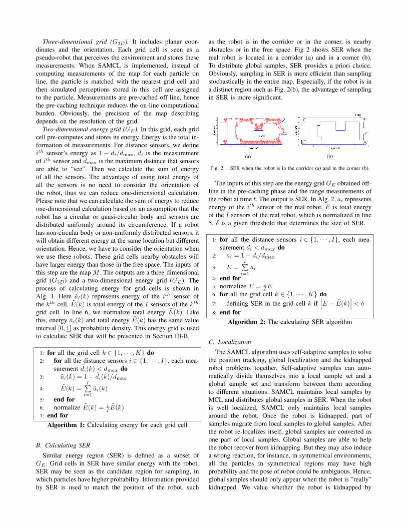
Two-dimensional energy grid (GE). In this grid, each gridcell pre-computes and stores its energy. Energy is the total in-formation of measurements. For distance sensors, we defineith sensor’s energy as 1 − di/dmax, di is the measurementof ith sensor and dmax is the maximum distance that sensorsare able to “see”. Then we calculate the sum of energyof all the sensors. The advantage of using total energy ofall the sensors is no need to consider the orientation ofthe robot, thus we can reduce one-dimensional calculation.Please note that we can calculate the sum of energy to reduceone-dimensional calculation based on an assumption that therobot has a circular or quasi-circular body and sensors aredistributed uniformly around its circumference. If a robothas non-circular body or non-uniformly distributed sensors, itwill obtain different energy at the same location but differentorientation. Hence, we have to consider the orientation whenwe use these robots. These grid cells nearby obstacles willhave larger energy than those in the free space. The inputs ofthis step are the map M . The outputs are a three-dimensionalgrid (G3D) and a two-dimensional energy grid (GE). Theprocess of calculating energy for grid cells is shown inAlg. 1. Here ai(k) represents energy of the ith sensor ofthe kth cell, E(k) is total energy of the I sensors of the kth

grid cell. In line 6, we normalize total energy E(k). Likethis, energy ai(k) and total energy E(k) has the same valueinterval [0, 1] as probability density. This energy grid is usedto calculate SER that will be presented in Section III-B.

1: for all the grid cell k ∈ {1, · · · ,K} do2: for all the distance sensors i ∈ {1, · · · , I}, each mea-

surement di(k) < dmax do3: ai(k) = 1− di(k)/dmax

4: E(k) =I∑

i=1

ai(k)

5: end for6: normalize E(k) = 1

I E(k)7: end for

Algorithm 1: Calculating energy for each grid cell

B. Calculating SER

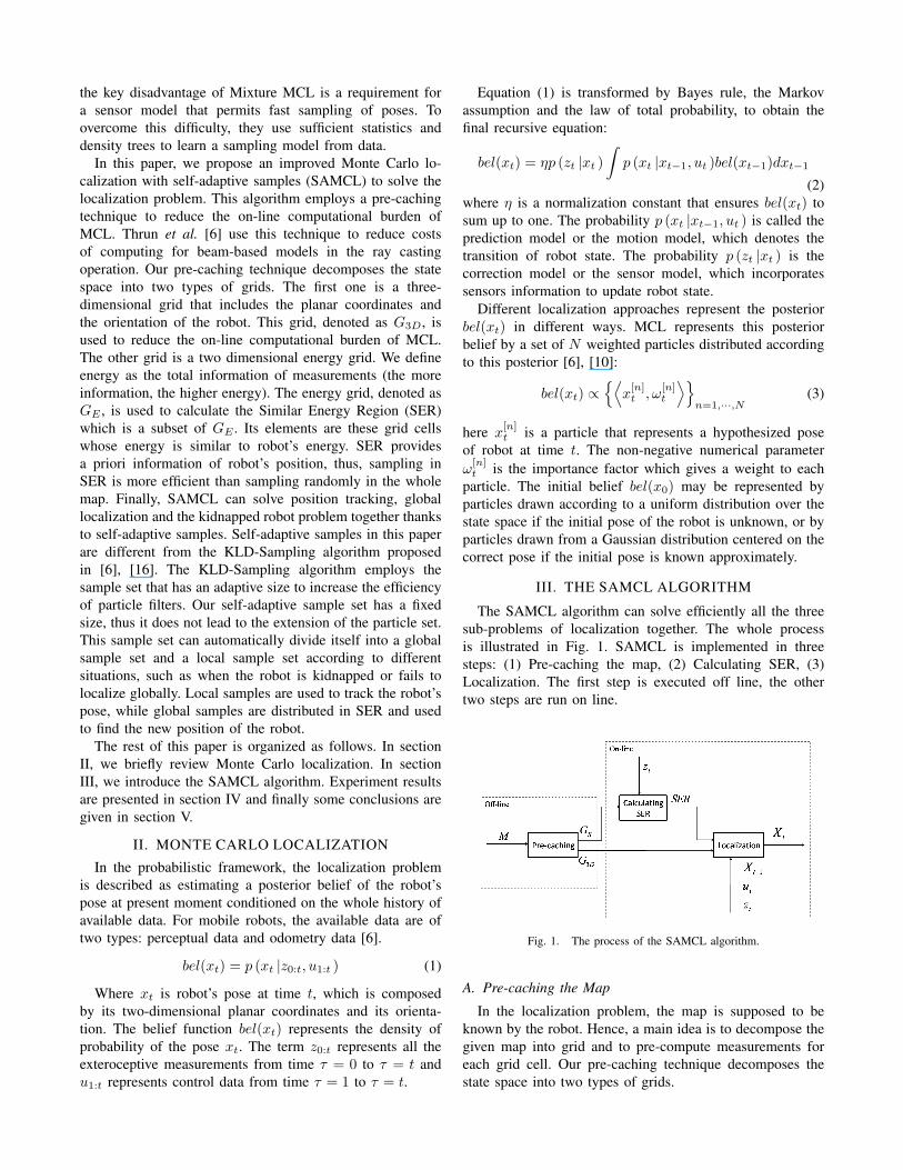
Similar energy region (SER) is defined as a subset ofGE . Grid cells in SER have similar energy with the robot.SER may be seen as the candidate region for sampling, inwhich particles have higher probability. Information providedby SER is used to match the position of the robot, such

as the robot is in the corridor or in the corner, is nearbyobstacles or in the free space. Fig 2 shows SER when thereal robot is located in a corridor (a) and in a corner (b).To distribute global samples, SER provides a priori choice.Obviously, sampling in SER is more efficient than samplingstochastically in the entire map. Especially, if the robot is ina distinct region such as Fig. 2(b), the advantage of samplingin SER is more significant.

(a) (b)

Fig. 2. SER when the robot is in the corridor (a) and in the corner (b).

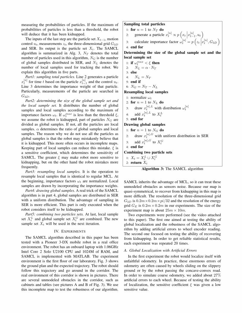
The inputs of this step are the energy grid GE obtained off-line in the pre-caching phase and the range measurements ofthe robot at time t. The output is SER. In Alg. 2, ai representsenergy of the ith sensor of the real robot, E is total energyof the I sensors of the real robot, which is normalized in line5. δ is a given threshold that determines the size of SER.

1: for all the distance sensors i ∈ {1, · · · , I}, each mea-surement di < dmax do

2: ai = 1− di/dmax

3: E =I∑

i=1

ai

4: end for5: normalize E = 1

IE6: for all the grid cell k ∈ {1, · · · ,K} do7: defining SER in the grid cell k if

∣∣∣E − E(k)∣∣∣ < δ

8: end forAlgorithm 2: The calculating SER algorithm

C. Localization

The SAMCL algorithm uses self-adaptive samples to solvethe position tracking, global localization and the kidnappedrobot problems together. Self-adaptive samples can auto-matically divide themselves into a local sample set and aglobal sample set and transform between them accordingto different situations. SAMCL maintains local samples byMCL and distributes global samples in SER. When the robotis well localized, SAMCL only maintains local samplesaround the robot. Once the robot is kidnapped, part ofsamples migrate from local samples to global samples. Afterthe robot re-localizes itself, global samples are converted asone part of local samples. Global samples are able to helpthe robot recover from kidnapping. But they may also inducea wrong reaction, for instance, in symmetrical environments,all the particles in symmetrical regions may have highprobability and the pose of robot could be ambiguous. Hence,global samples should only appear when the robot is ”really”kidnapped. We value whether the robot is kidnapped by

measuring the probabilities of particles. If the maximum ofprobabilities of particles is less than a threshold, the robotwill deduce that it has been kidnapped.

The inputs of the last step are the particle set Xt−1, motioncontrol ut, measurements zt, the three-dimensional grid G3D

and SER. Its output is the particle set Xt. The SAMCLalgorithm is summarized in Alg. 3, NT denotes the totalnumber of particles used in this algorithm, NG is the numberof global samples distributed in SER, and NL denotes thenumber of local samples used for tracking the robot. Weexplain this algorithm in five parts.

Part1: sampling total particles. Line 2 generates a particlex

[n]t for time t based on the particle x[n]

t−1 and the control ut.Line 3 determines the importance weight of that particle.Particularly, measurements of the particle are searched inG3D.

Part2: determining the size of the global sample set andthe local sample set. It distributes the number of globalsamples and local samples according to the maximum ofimportance factors ωt. If ωmax

t is less than the threshold ξ,we assume the robot is kidnapped, part of particles NG aredivided as global samples. If not, all the particles are localsamples. α determines the ratio of global samples and localsamples. The reason why we do not use all the particles asglobal samples is that the robot may mistakenly believe thatit is kidnapped. This more often occurs in incomplete maps.Keeping part of local samples can reduce this mistake. ξ isa sensitive coefficient, which determines the sensitivity ofSAMCL. The greater ξ may make robot more sensitive tokidnapping, but on the other hand the robot mistakes morefrequently.

Part3: resampling local samples. It is the operation toresample local samples that is identical to regular MCL. Atthe beginning, importance factors ωt are normalized. Localsamples are drawn by incorporating the importance weights.

Part4: drawing global samples. A real trick of the SAMCLalgorithm is in part 4, global samples are distributed in SERwith a uniform distribution. The advantage of sampling inSER is more efficient. This part is only executed when therobot considers itself to be kidnapped.

Part5: combining two particles sets. At last, local sampleset XL

t and global sample set XGt are combined. The new

sample set Xt will be used in the next iteration.

IV. EXPERIMENTS

The SAMCL algorithm described in this paper has beentested with a Pioneer 3-DX mobile robot in a real officeenvironment. The robot has an onboard laptop with 1.06GHzIntel Core 2 Solo U2100 CPU and 1024M of RAM, andSAMCL is implemented with MATLAB. The experimentenvironment is the first floor of our laboratory. Fig. 3 showsthe ground plan and the expected trajectory. The robot shouldfollow this trajectory and go around in the corridor. Thereal environment of this corridor is shown in pictures. Thereare several unmodeled obstacles in the corridor, such ascabinets and tables (see pictures A and B of Fig. 3). We usethis incomplete map to test the robustness of our algorithm.

Sampling total particles1: for n = 1 to NT do2: generate a particle x[n]

t ∝ p(xt

∣∣∣x[n]t−1, ut

)3: calculate importance factor ω[n]

t = p(zt

∣∣∣x[n]t , G3D

)4: end for

Determining the size of the global sample set and thelocal sample set

1: if ωmaxt < ξ then

2: NL = α ·NT

3: else4: NL = NT

5: end if6: NG = NT −NL

Resampling local samples1: normalize ωt

2: for n = 1 to NL do3: draw x

[n],Lt with distribution ω[n]

t

4: add x[n],Lt to XL

t

5: end forDrawing global samples

1: for n = 1 to NG do2: draw x

[n],Gt with uniform distribution in SER

3: add x[n],Gt to XG

t

4: end forCombining two particle sets

1: Xt = XLt ∪XG

t

2: return Xt

Algorithm 3: The SAMCL algorithm

SAMCL inherits the advantage of MCL, so it can treat theseunmodeled obstacles as sensors noise. Because our map isquasi-symmetrical, to recover from kidnapping in this map ismore difficult. The resolution of the three-dimensional gridG3D is 0.2m×0.2m×pi/32 and the resolution of the energygrid GE is 0.2m×0.2m in our experiments. The size of theexperiment map is about 25m× 10m.

Two experiments were performed (see the video attachedto this paper). The first one aimed at testing the ability ofglobal localization and the robustness of the SAMCL algo-rithm by adding artificial errors to wheel encoder reading.The second one focused on testing the ability of recoveringfrom kidnapping. In order to get reliable statistical results,each experiment was repeated 20 times.

A. Global Localization with Artificial Errors

In the first experiment the robot would localize itself withunfaithful odometry. In practice, these enormous errors ofodometry are often caused by wheels sliding on the slipperyground or by the robot passing the concave-convex road.In order to simulate coarse odometry, we added about 27%artificial errors to each wheel. Because of testing the abilityof localization, the sensitive coefficient ξ was given a lowsensitive value.

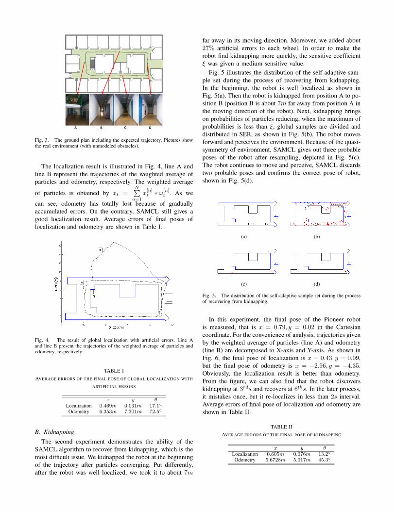
Fig. 3. The ground plan including the expected trajectory. Pictures showthe real environment (with unmodeled obstacles).

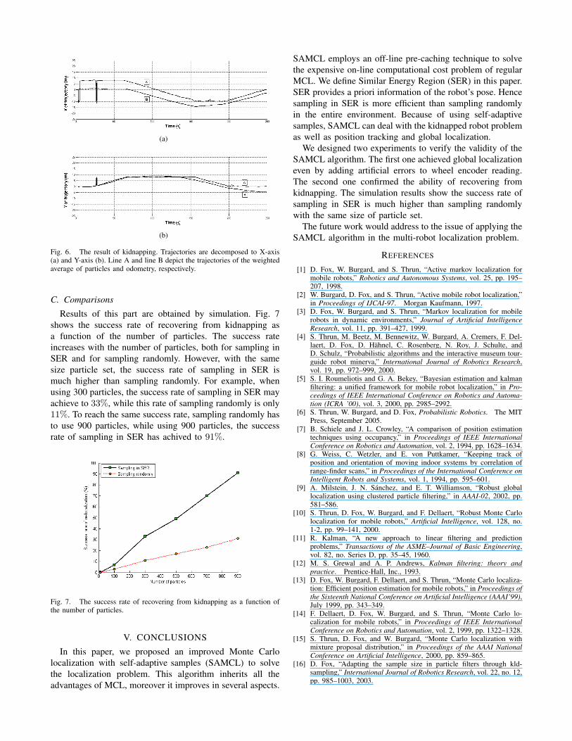
The localization result is illustrated in Fig. 4, line A andline B represent the trajectories of the weighted average ofparticles and odometry, respectively. The weighted average

of particles is obtained by xt =N∑

n=1x

[n]t ∗ ω

[n]t . As we

can see, odometry has totally lost because of graduallyaccumulated errors. On the contrary, SAMCL still gives agood localization result. Average errors of final poses oflocalization and odometry are shown in Table I.

Fig. 4. The result of global localization with artificial errors. Line Aand line B present the trajectories of the weighted average of particles andodometry, respectively.

TABLE IAVERAGE ERRORS OF THE FINAL POSE OF GLOBAL LOCALIZATION WITH

ARTIFICIAL ERRORS

x y θLocalization 0.469m 0.031m 17.1◦

Odometry 6.353m 7.301m 72.5◦

B. Kidnapping

The second experiment demonstrates the ability of theSAMCL algorithm to recover from kidnapping, which is themost difficult issue. We kidnapped the robot at the beginningof the trajectory after particles converging. Put differently,after the robot was well localized, we took it to about 7m

far away in its moving direction. Moreover, we added about27% artificial errors to each wheel. In order to make therobot find kidnapping more quickly, the sensitive coefficientξ was given a medium sensitive value.

Fig. 5 illustrates the distribution of the self-adaptive sam-ple set during the process of recovering from kidnapping.In the beginning, the robot is well localized as shown inFig. 5(a). Then the robot is kidnapped from position A to po-sition B (position B is about 7m far away from position A inthe moving direction of the robot). Next, kidnapping bringson probabilities of particles reducing, when the maximum ofprobabilities is less than ξ, global samples are divided anddistributed in SER, as shown in Fig. 5(b). The robot movesforward and perceives the environment. Because of the quasi-symmetry of environment, SAMCL gives out three probableposes of the robot after resampling, depicted in Fig. 5(c).The robot continues to move and perceive, SAMCL discardstwo probable poses and confirms the correct pose of robot,shown in Fig. 5(d).

(a) (b)

(c) (d)

Fig. 5. The distribution of the self-adaptive sample set during the processof recovering from kidnapping.

In this experiment, the final pose of the Pioneer robotis measured, that is x = 0.79, y = 0.02 in the Cartesiancoordinate. For the convenience of analysis, trajectories givenby the weighted average of particles (line A) and odometry(line B) are decomposed to X-axis and Y-axis. As shown inFig. 6, the final pose of localization is x = 0.43, y = 0.09,but the final pose of odometry is x = −2.96, y = −4.35.Obviously, the localization result is better than odometry.From the figure, we can also find that the robot discoverskidnapping at 3rds and recovers at 6ths. In the later process,it mistakes once, but it re-localizes in less than 2s interval.Average errors of final pose of localization and odometry areshown in Table II.

TABLE IIAVERAGE ERRORS OF THE FINAL POSE OF KIDNAPPING

x y θLocalization 0.605m 0.076m 13.2◦

Odometry 5.6728m 5.017m 45.3◦

(a)

(b)

Fig. 6. The result of kidnapping. Trajectories are decomposed to X-axis(a) and Y-axis (b). Line A and line B depict the trajectories of the weightedaverage of particles and odometry, respectively.

C. Comparisons

Results of this part are obtained by simulation. Fig. 7shows the success rate of recovering from kidnapping asa function of the number of particles. The success rateincreases with the number of particles, both for sampling inSER and for sampling randomly. However, with the samesize particle set, the success rate of sampling in SER ismuch higher than sampling randomly. For example, whenusing 300 particles, the success rate of sampling in SER mayachieve to 33%, while this rate of sampling randomly is only11%. To reach the same success rate, sampling randomly hasto use 900 particles, while using 900 particles, the successrate of sampling in SER has achived to 91%.

Fig. 7. The success rate of recovering from kidnapping as a function ofthe number of particles.

V. CONCLUSIONS

In this paper, we proposed an improved Monte Carlolocalization with self-adaptive samples (SAMCL) to solvethe localization problem. This algorithm inherits all theadvantages of MCL, moreover it improves in several aspects.

SAMCL employs an off-line pre-caching technique to solvethe expensive on-line computational cost problem of regularMCL. We define Similar Energy Region (SER) in this paper.SER provides a priori information of the robot’s pose. Hencesampling in SER is more efficient than sampling randomlyin the entire environment. Because of using self-adaptivesamples, SAMCL can deal with the kidnapped robot problemas well as position tracking and global localization.

We designed two experiments to verify the validity of theSAMCL algorithm. The first one achieved global localizationeven by adding artificial errors to wheel encoder reading.The second one confirmed the ability of recovering fromkidnapping. The simulation results show the success rate ofsampling in SER is much higher than sampling randomlywith the same size of particle set.

The future work would address to the issue of applying theSAMCL algorithm in the multi-robot localization problem.

REFERENCES

[1] D. Fox, W. Burgard, and S. Thrun, “Active markov localization formobile robots,” Robotics and Autonomous Systems, vol. 25, pp. 195–207, 1998.

[2] W. Burgard, D. Fox, and S. Thrun, “Active mobile robot localization,”in Proceedings of IJCAI-97. Morgan Kaufmann, 1997.

[3] D. Fox, W. Burgard, and S. Thrun, “Markov localization for mobilerobots in dynamic environments,” Journal of Artificial IntelligenceResearch, vol. 11, pp. 391–427, 1999.

[4] S. Thrun, M. Beetz, M. Bennewitz, W. Burgard, A. Cremers, F. Del-laert, D. Fox, D. Hahnel, C. Rosenberg, N. Roy, J. Schulte, andD. Schulz, “Probabilistic algorithms and the interactive museum tour-guide robot minerva,” International Journal of Robotics Research,vol. 19, pp. 972–999, 2000.

[5] S. I. Roumeliotis and G. A. Bekey, “Bayesian estimation and kalmanfiltering: a unified framework for mobile robot localization,” in Pro-ceedings of IEEE International Conference on Robotics and Automa-tion (ICRA ’00), vol. 3, 2000, pp. 2985–2992.

[6] S. Thrun, W. Burgard, and D. Fox, Probabilistic Robotics. The MITPress, September 2005.

[7] B. Schiele and J. L. Crowley, “A comparison of position estimationtechniques using occupancy,” in Proceedings of IEEE InternationalConference on Robotics and Automation, vol. 2, 1994, pp. 1628–1634.

[8] G. Weiss, C. Wetzler, and E. von Puttkamer, “Keeping track ofposition and orientation of moving indoor systems by correlation ofrange-finder scans,” in Proceedings of the International Conference onIntelligent Robots and Systems, vol. 1, 1994, pp. 595–601.

[9] A. Milstein, J. N. Sanchez, and E. T. Williamson, “Robust globallocalization using clustered particle filtering,” in AAAI-02, 2002, pp.581–586.

[10] S. Thrun, D. Fox, W. Burgard, and F. Dellaert, “Robust Monte Carlolocalization for mobile robots,” Artificial Intelligence, vol. 128, no.1-2, pp. 99–141, 2000.

[11] R. Kalman, “A new approach to linear filtering and predictionproblems,” Transactions of the ASME–Journal of Basic Engineering,vol. 82, no. Series D, pp. 35–45, 1960.

[12] M. S. Grewal and A. P. Andrews, Kalman filtering: theory andpractice. Prentice-Hall, Inc., 1993.

[13] D. Fox, W. Burgard, F. Dellaert, and S. Thrun, “Monte Carlo localiza-tion: Efficient position estimation for mobile robots,” in Proceedings ofthe Sixteenth National Conference on Artificial Intelligence (AAAI’99),July 1999, pp. 343–349.

[14] F. Dellaert, D. Fox, W. Burgard, and S. Thrun, “Monte Carlo lo-calization for mobile robots,” in Proceedings of IEEE InternationalConference on Robotics and Automation, vol. 2, 1999, pp. 1322–1328.

[15] S. Thrun, D. Fox, and W. Burgard, “Monte Carlo localization withmixture proposal distribution,” in Proceedings of the AAAI NationalConference on Artificial Intelligence, 2000, pp. 859–865.

[16] D. Fox, “Adapting the sample size in particle filters through kld-sampling,” International Journal of Robotics Research, vol. 22, no. 12,pp. 985–1003, 2003.