Fluid Phase Equilibria 230 (2005) 121–130

Liquid–liquid equilibria for pseudoternary systems:isooctane–benzene–(methanol + water)

Blanca Estela Garcıa-Floresa,b, Monica Gramajo de Doza,1, Arturo Trejoa,∗a Instituto Mexicano del Petr´oleo, Programa de Ingenier´ıa Molecular, Ciencias Basicas, Eje L´azaro Cardenas 152, 07730 M´exico D.F., Mexico

b Area de Investigaci´on en Termof´ısica, Eje Lazaro Cardenas 152, 07730 M´exico D.F., Mexico

Received 30 April 2004; received in revised form 7 December 2004; accepted 8 December 2004Available online 21 January 2005

Abstract

Liquid–liquid equilibrium data are presented for the pseudoternary systems isooctane–benzene–(90 mass% methanol + 10 mass% water)at 298.15 K and isooctane–benzene–(80 mass% methanol + 20 mass% water) at 298.15 and 308.15 K, under atmospheric pressure. The ex-perimental tie-line data obtained define the binodal curve for each one of the studied systems which depending on the amount of waterpresent show type I or type II liquid–liquid phase diagrams. In order to obtain a general view of the effect of water on the partitioning ofm the systemi tie-line dataf n of thee©

K

1

uirgmtadspap

thendtificut-

dy ofiumcar-partsethe

ol inout

undergaing of

ib-xedar-

0d

ethanol and hence on the size of the two-phase region we have also determined experimentally ‘isowater’ tolerance curves forsooctane–benzene–methanol at 298.15 K, hence the tie-line data were also obtained for the ternary system. The experimentalor the four systems studied were correlated with the NRTL and UNIQUAC solution models obtaining a very good reproductioxperimental behaviour.2004 Elsevier B.V. All rights reserved.

eywords:Experiments; Hydrocarbons; Isowater curves; Liquid–liquid equilibrium; Methanol; Tie-lines

. Introduction

In recent years, there has been an increasing demand tose oxygenated compounds in the reformulation of gasoline

n order to substantially reduce toxic emissions into the envi-onment and simultaneously enhance the octane number ofasoline. The physical and chemical properties of methanolake it an excellent candidate as an oxygenated fuel addi-

ive. Some advantages obtained from using methanol are: itsnti-knocking properties, high oxygen content, it can be pro-uced from a relatively large variety of carbon-based feed-tocks and relatively low cost. However, methanol presentsartial miscibility with aliphatic hydrocarbons, not so withromatics. Additionally, in the reformulation of gasoline, theresence of water, even in traces, should always be consid-

∗ Corresponding author. Tel.: +52 55 91758373; fax: +52 55 91756439.E-mail address:atrejo@imp.mx (A. Trejo).

1 Permanent address: Universidad Nacional de Tucuman, Argentina.

ered. Hence, the knowledge of the effect of water onpartial miscibility of methanol in mixtures of aliphatic aaromatic hydrocarbons is of interest from both the scienand the technological points of view. It is therefore ofmost importance to undertake the creation a reliable boexperimental results on the liquid–liquid phase equilibrof systems composed of methanol and different hydrobons representative of gasoline with the principal aim, afrom the intrinsic interest of the study of liquid–liquid phadiagrams of multi-component systems, of establishingconcentration interval of both hydrocarbons and methanwhich the two-phase region does not exist with and withthe presence of water at a given constant temperature,atmospheric pressure. Part of the same objective is toknowledge on the effect of temperature on the partitioninmethanol between the equilibrium phases.

In this work we chose to study the liquid–liquid equilrium related to the study of the solubility of methanol miwith different amounts of water in mixtures of two hydroc

378-3812/$ – see front matter © 2004 Elsevier B.V. All rights reserved.

oi:10.1016/j.fluid.2004.12.003

122 B.E. Garc´ıa-Flores et al. / Fluid Phase Equilibria 230 (2005) 121–130

bons: isooctane and benzene. We have investigated the phaseequilibrium of the systems isooctane–benzene–(90 mass%methanol + 10 mass% water) at 298.15 K and isooctane–benzene–(80 mass% methanol + 20 mass% water) at 298.15and 308.15 K. Although the results of this work correspondto quaternary systems, we present them as pseudoternarysystems. The experimental tie-line data for the differentpseudoternary systems and for the ternary system withoutwater were successfully correlated with the NRTL and UNI-QUAC solution models. Also, with a view to establish thegeneral effect of water on the liquid–liquid behaviour of theternary system composed of isooctane–benzene–methanolwe have determined experimentally the solubility regions or‘isowater’ tolerance curves at 298.15 K.

2. Experimental

2.1. Materials

The samples of methanol and benzene were supplied byBaker, whereas isooctane was provided by Sigma Aldrich.All the samples were HPLC grade and their purity is reportedby the supplier to be higher than 99 mol%. They were usedwithout any further purification. No impurities were detectedusing gas chromatography with a thermal conductivity de-t ry tod m-i dro-c thanolw f wa-t tookt ara-t undto

2c

urveso imi-l thel mo at de-s ndC amo s de-ta n isp atedm ingea oudp h thec dif-f MP,

Fig. 1. Liquid–liquid equilibrium cell for the determination of water toler-ance curves.

with a precision and accuracy of±0.0001 g. This proce-dure was repeated as many times as necessary to obtainenough cloud points results that mapped out the whole re-gion above the binodal curve of the corresponding ternarysystem. The temperature of the cell was controlled with aconstant temperature bath-circulator at the temperatures re-ported in this work with a stability of±0.01 K, as mea-sured with a digital thermometer with platinum resistanceprobe.

Starting with five completely miscible binaries ofisooctane–benzene of known constant mass ratio, i.e. isooc-tane/benzene = 85/15, 75/25, 60/40, 45/55, 30/70, 15/85 and5/95, different known amounts of methanol were added inorder to have 35 ternary miscible mixtures with differentwell-known concentration. The mass of each component ofthe binaries was determined in 10 cm3 vials using the sameanalytical balance as above whereas that of methanol was de-termined by mass difference in the same analytical balance.The total miscible range of the ternary system was coveredwith 35 experimental points, including several cloud pointsfor the binary benzene–methanol mixture. With all the knownvalues of the concentration of the ternary miscible mixturesand the results corresponding to the amount of water addedto observe the cloud point in each ternary mixture a plot ofmass of water versus mass of methanol was prepared to ob-tain different curves each one identified by the mass% ratio ofi masso oughv d re-p rnarys

ector (TCD), except for isooctane, which was necessaistill in an all glass column at high reflux in order to eli

nate impurities. The water used was deionized. The hyarbon samples were stored over sodium whereas meas stored over molecular sieve spheres. The amount o

er in each pure sample was monitored along the time ito carry out the present study with a Karl–Fisher appus, Aquatest 8, Photovolt. Methanol was the only compohat had water; it contained a maximum of 3× 10−3 mass%f water.

.2. Measurement of water tolerance or cloud pointurves

The experimental measurement of water tolerance cr ‘isowater’ curves was carried out in glass cells, s

ar to the ones used also in this work for the study ofiquid–liquid equilibrium.Fig. 1shows a schematic diagraf a cell. The experimental procedure is the same as thcribed in previous work[1] based on the work by Briggs aomings[2]. In a first stage the liquid–liquid phase diagrf the ternary isooctane–benzene–methanol system wa

ermined as explained in the next section. About 10 cm3 ofhomogeneous ternary mixture of known concentratio

laced in the glass cell and vigorously stirred by a coagnetic bar. Then, water was added slowly from a syrnd stirring was applied almost continuously until the cloint was observed. The mass of water added to reacloud point of the system was determined from masserences with an analytical balance, Sartorious 2006

sooctane to benzene. From this plot different constantf water values were selected in order to interpolate enalues to fully describe the water tolerance behaviour anort isowater values as mass of water per 10 g of the teystem.

B.E. Garc´ıa-Flores et al. / Fluid Phase Equilibria 230 (2005) 121–130 123

2.3. Measurement of liquid–liquid equilibrium

For the study of the liquid–liquid equilibrium ofboth ternary (isooctane–benzene–methanol) and quaternary(isooctane–benzene–(methanol + water)) systems the mea-surements were carried out in the same type of cells reportedin the work by Romero-Martınez and Trejo[3] and used inprevious work[1]. The main difference between this cell andthat illustrated inFig. 1 is that the liquid–liquid equilibriumcell has capillary ports to sample the phases. Disposable sy-ringes were adapted to the sampling ports of the equilibriumcells at the beginning of each experimental run and great carewas taken to eliminate dead spaces along the glass capillar-ies that link the cells and the syringes. Each multi-componentsystem of known concentration was collocated in an equilib-rium cell and stirred by a magnetic bar during a minimumperiod of 4 h, then allowed to settle for a 10 h period to ob-tain two liquid phases in equilibrium, one hydrocarbon-richand the other water–methanol-rich. Both equilibrium phaseswere sampled with the disposable syringes and analyzed ina Varian Model 3400 chromatograph using a TCD and a Po-rapak Q column obtaining results that possess excellent re-producibility. Several tie-lines were determined as to definecompletely the binodal curve for each studied system at con-stant temperature. The reported concentration results are theaverage of at least four injections of the same sample into thec

ibra-t re-p ardw eousm incet con-t haveb How-e ion,o cor-r po-n egiono erentr nce,t e tol theo e re-s ter-n cribedi ory[

w ali-b eachc

w

Table 1Values of the parameters for the chromatographic calibration curve (Eq.(1))for the different systems investigated

Component m R

System: isooctane–benzene–methanolIsooctane 0.9654 0.9996Benzene 1.0593 0.9995Methanol 1.4062 0.9998

System: isooctane–benzene–(90 mass% methanol + 10 mass% water)Isooctane 0.8530 0.9994Benzene 0.8904 0.9993Methanol 0.9468 0.9994Water 1.1839 0.9998

System: isooctane–benzene–(80 mass% methanol + 20 mass% water)Isooctane 0.8592 0.9995Benzene 0.8827 0.9994Methanol 0.7653 0.9999Water 0.5278 0.9998

R is the correlation coefficient for each fit.

wherewi is the mass of thei component of the system,Aithe chromatographic area of the componenti, As the chro-matographic area of the internal standard,ws the mass of theinternal standard andb andm the ordinate and the slope ofthe fitted straight line, respectively.

It can be observed inTable 1that as expectedb= 0 for allthe calibration equations obtained.

3. Results and discussion

3.1. Liquid–liquid equilibrium of the ternary system

As mentioned in Section2.2 in order to carry out themeasurements of cloud points of water in the ternary sys-tem formed by isooctane–benzene–methanol it was nec-essary first to define the binodal curve for this systemunder isothermal conditions, since this information wouldhelp to establish the totally miscible region to prepare theternary mixtures of known concentration. The experimen-tal tie-line data in mass fraction for the ternary systemof isooctane–benzene–methanol at 298.15 K, are given inTable 2and also shown graphically inFig. 2. It is possible tosee from the latter that the partial miscibility region is rela-tively small, so that it can be inferred that the formulation of

TEt –(3)m

H

x

0 00000 01590 03500 06200 0739

hromatograph.The internal standard method was used for the cal

ion of the TCD’s response in order to achieve highroducibility. A constant amount of the internal standas used in each one of the vials where the homogenulti-component mixtures were prepared as follows. S

he two pseudoternary systems studied in this workain the same components a single calibration wouldeen enough to carry out the chromatographic analysis.ver, multi-component mixtures, i.e. in the miscible regf known concentration were prepared to obtain theesponding calibration curve for each of the four coments for each phase diagram, since the two-phase rf each studied pseudoternary system covers quite diffanges of concentration as will be observed below. Hehis method avoids extrapolations that would give risarge uncertainties in the concentration values and onther hand guarantees a high accuracy of the tie-linults for each particular system. In this study, the inal standard was ethanol. This method has been des

n essential detail in a previous work from our laborat1].

The values of the parameters in Eq.(1)are given inTable 1,hich correspond to the fitting of the chromatographic cration obtained using the internal standard method foromponent of each system studied.

i =(

Ai

As− b

) (ws

m

)(1)

able 2xperimental values of concentration, in mole (x) and mass fraction (w), for

he liquid–liquid equilibrium of the system (1) isooctane–(2) benzeneethanol at 298.15 K

ydrocarbon-rich phase Methanol-rich phase

1 x2 w1 w2 x1 x2 w1 w2

.7720 0.0000 0.9235 0.0000 0.1184 0.0000 0.3280 0.

.7391 0.0207 0.9006 0.0172 0.1238 0.0087 0.3318 0.

.6873 0.0418 0.8679 0.0361 0.1447 0.0201 0.3686 0.

.6030 0.0678 0.8130 0.0625 0.1803 0.0386 0.4234 0.

.5184 0.0754 0.7580 0.0754 0.2022 0.0481 0.4540 0.

124 B.E. Garc´ıa-Flores et al. / Fluid Phase Equilibria 230 (2005) 121–130

Fig. 2. Experimental water tolerance curves for the system (w1)isooctane–(w2) benzene–(w3) methanol at 298.15 K. Concentrations are inmass fraction. Experimental liquid–liquid equilibrium results for the ternarysystem at 298.15 K: (�). Tolerance curves are identified by mass of water ingrams per 10 g of ternary system.

gasoline with the right amount of methanol would not showphase separation.

Our experimental tie-line results in mole fraction for theternary isooctane–benzene–methanol were compared withreported data by Higashiuchi et al.[4] at the same temper-ature. This comparison is shown inFig. 3. Good agreementis observed within the experimental uncertainty of both datasets.

3.2. Water tolerance curves

For the experimental determination of the cloud points ofwater in the above mentioned ternary system different bi-nary systems of isooctane–benzene were used as base for thepreparation of the ternary completely miscible mixtures ofknown concentration. They had the following mass fractionratio (isooctane/benzene): 85/15, 75/25, 60/40, 45/55, 30/70,15/85 and 5/95.Table 3gives the results of mass of water,in grams, to observe the cloud point in 10 g of ternary sys-tem. Also included inTable 3are values of concentration,in mass fraction, of each system at the cloud point. Somevalues, i.e. 17 points, for the mass of water were interpolatedusing empirical polynomial equations in order to report com-plete different tolerance curves, i.e. isowater tolerance curves.

F thes ra-t

Table 3Experimental values for the mass of water needed to observe cloud pointsin 10 g of the system isooctane–benzene–methanol at 298.15 K

Water (g) Water Methanol Benzene Isooctane

Binary with 85/15 mass% ratio0.010 0.0010 0.3247 0.1009 0.57340.020 0.0020 0.4686 0.0798 0.44970.030 0.0030 0.5184 0.0718 0.40680.040 0.0040 0.5578 0.0657 0.37250.060 0.0566 0.8491 0.0142 0.08020.080 0.0741 0.8333 0.0139 0.0787

Binary with 60/40 mass% ratio0.060 0.0060 0.2187 0.3101 0.46520.080 0.0079 0.3075 0.2738 0.41070.100 0.0099 0.3713 0.2475 0.37130.200 0.0196 0.5755 0.1618 0.24310.400 0.0385 0.7087 0.1010 0.15190.600 0.0566 0.7708 0.0689 0.10380.800 0.0741 0.8056 0.0481 0.07221.000 0.0909 0.8182 0.0364 0.0545

Binary with 30/70 mass% ratio0.200 0.01961 0.25294 0.50882 0.218630.400 0.03842 0.43708 0.36695 0.157540.600 0.05660 0.56604 0.26415 0.113210.800 0.07407 0.64074 0.20000 0.085191.000 0.09083 0.68574 0.15622 0.06721

Binary with 5/95 mass% ratio0.200 0.0196 0.1863 0.7539 0.04020.400 0.0385 0.2981 0.6298 0.03370.600 0.0566 0.3840 0.5311 0.02830.800 0.0741 0.4519 0.4500 0.02411.000 0.0909 0.5045 0.3845 0.02002.000 0.1667 0.6208 0.2017 0.0108

Binary with 75/25 mass% ratio0.040 0.0040 0.3881 0.1522 0.45570.060 0.0060 0.5020 0.1233 0.36880.080 0.0079 0.5585 0.1081 0.32540.100 0.0099 0.5955 0.0989 0.29570.200 0.0196 0.6912 0.0725 0.21670.400 0.0385 0.7567 0.0510 0.15380.600 0.0566 0.7936 0.0377 0.11220.800 0.0741 0.8176 0.0269 0.0815

Binary with 45/55 mass% ratio0.080 0.0079 0.1587 0.4583 0.37500.100 0.0099 0.1980 0.4356 0.35640.200 0.0196 0.3657 0.3382 0.27650.400 0.0385 0.6008 0.1983 0.16250.600 0.0566 0.6934 0.1377 0.11230.800 0.0741 0.7398 0.1028 0.08331.000 0.0909 0.7682 0.0773 0.0636

Binary with 15/85 mass% ratio0.200 0.0196 0.2206 0.6461 0.11370.400 0.0385 0.3529 0.5173 0.09130.600 0.0566 0.4430 0.4251 0.07540.800 0.0741 0.5185 0.3463 0.06111.000 0.0909 0.5773 0.2818 0.05002.000 0.1665 0.6744 0.1349 0.0241

Binary: benzene–methanol0.200 0.0196 0.1716 0.80880.400 0.0385 0.2808 0.68080.600 0.0566 0.3679 0.57550.800 0.0741 0.4278 0.4981

ig. 3. Comparison of experimental liquid–liquid equilibrium results forystem (x1) isooctane–(x2) benzene–(x3) methanol at 298.15 K. Concentions are in mole fraction. This work (�); Higashiuchi et al. (1990) (�).

B.E. Garc´ıa-Flores et al. / Fluid Phase Equilibria 230 (2005) 121–130 125

Table 3 (Continued)

Water (g) Water Methanol Benzene Isooctane

1.000 0.0909 0.4736 0.43552.000 0.1667 0.5917 0.2417

Values of concentration in mass fraction are given for each system. Theresults are identified for each binary of isooctane–benzene with its mass%ratio.

It is worth to notice that several points for different isowa-ter curves are included for the binary benzene–methanol,which help to fully define several curves. InFig. 2the corre-sponding isowater tolerance curves together with the binodalcurve for the ternary system are depicted. For very smallamounts of water (up to 0.03 g), the cloud points (bound-ary of liquid–liquid immiscibility) falls on the binodal curvethat was determined in the absence of water. However, start-ing with 0.04 g of water the region of partial miscibility in-creases as the amount of water increases. On the other ex-treme of isowater values it is observed that for 2 g of water inthe ternary system the immiscibility is almost total. InFig. 2we have thus identified the two liquid-phase region of theternary with the binodal curve and the different isowater tol-erance curves, for which the right hand side represents totalmiscibility whereas the left hand side represents partial mis-cibility.

These results are consistent with those reported inthe works by Terzoni et al.[5] and Ancillotti andPescarollo [6], in which water tolerance curves weredetermined for the systems isooctane–toluene–methanoland isooctane–toluene–methanol–methyltert-butyl ether(MTBE). Also, in previous work[1] we presented a studyon water tolerance curves for the ternary system isooctane–o-xylene–methanol at 298.15 K. The results showed similar be-haviour as that discussed above for the system studied in thisw e ofa sys-t viourc arys enta-t res-e wa-t ossi-b untso in-c cleart rovedw con-c vante tem[

3

me-w s ofa l re-

sults obtained under controlled conditions allow an explo-ration of the complete range of concentration to identify themost critical regions of the phenomena under study, con-sequently the results do correspond to a close model forthe real system. Hence, we have also performed an exper-imental study of the liquid–liquid equilibrium for the sys-tem isooctane–benzene–methanol with water concentrationof 10 and 20 mass% in methanol in order to define boththe partial and total miscibility regions. The systems in-vestigated are in fact quaternary, although with the aimto represent the liquid–liquid phase behaviour in a directway, we will treat them as pseudoternaries in the followingway: isooctane–benzene–(90 mass% methanol + 10 mass%water) at 298.15 K and isooctane–benzene–(80 mass%methanol + 20 mass% water) at 298.15 and 308.15 K.

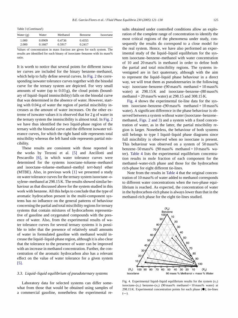
Fig. 4 shows the experimental tie-line data for the sys-tem isooctane–benzene–(90 mass% methanol + 10 mass%water). A significant difference in the phase behaviour is ob-served between a system without water (isooctane–benzene–methanol,Figs. 2 and 3) and a system with a fixed concen-tration of water, as in the latter, the partial miscibility re-gion is larger. Nonetheless, the behaviour of both systemsstill belongs to type I liquid–liquid phase diagrams sincefull miscibility is observed when no isooctane is present.This behaviour was observed on a system of 50 mass%benzene–50 mass% (90 mass% methanol + 10 mass% wa-t ra-t them rbonr

-t ondst qui-l ateri n them

F (i ) at2(

ork with benzene. All this helps to conclude that the typromatic hydrocarbon present in the multi-component

ems has no influence on the general patterns of behaoncerning the partial and total miscibility regions for ternystems that contain mixtures of hydrocarbons represive of gasoline and oxygenated compounds with the pnce of water. Also, from the experimental results of

er tolerance curves for several ternary systems it is ple to infer that the presence of relatively small amof water in formulated gasoline with methanol wouldrease the liquid–liquid-phase region, although it is alsohat the tolerance to the presence of water can be impith an increase in methanol concentration. Further, theentration of the aromatic hydrocarbon also has a releffect on the value of water tolerance for a given sys

5].

.3. Liquid–liquid equilibrium of pseudoternary systems

Laboratory data for selected systems can differ sohat from those that would be obtained using samplecommercial gasoline, nonetheless the experimenta

er). Table 4 lists the experimental equilibrium concention results in mole fraction of each component forethanol–water-rich phase and those for the hydroca

ich-phase for eight different tie-lines.Note from the results inTable 4that the original concen

ration of 10 mass% of water added to methanol correspo different water concentrations when the two-phase eibrium is reached. As expected, the concentration of wn the hydrocarbon-rich phase is always lower than that i

ethanol-rich phase for the eight tie-lines studied.

ig. 4. Experimental liquid–liquid equilibrium results for the systemx1)sooctane–(x2) benzene–(x3) (90 mass% methanol + 10 mass% water98.15 K. Experimental concentration points for each phase (�); tie-lines—).

126 B.E. Garc´ıa-Flores et al. / Fluid Phase Equilibria 230 (2005) 121–130

Table 4Experimental values of concentration, in mole fraction, for the liquid–liquid equilibrium of the pseudoternary system isooctane–benzene–(90 mass%methanol + 10 mass% water) at 298.15 K and isooctane–benzene–(80 mass% methanol + 20 mass% water) at 298.15 and 308.15 K

Tie-line Alcohol–water-rich phase Hydrocarbon-rich phase

xisooctane xbenzene xmethanol xwater xisooctane xbenzene xmethanol xwater

System isooctane–benzene–(90 mass% methanol + 10 mass% water) at 298.15 K1 0.0158 0.0000 0.8598 0.1244 0.9205 0.0000 0.0444 0.03512 0.0146 0.0115 0.8200 0.1539 0.8245 0.0787 0.0654 0.03153 0.0153 0.0124 0.8306 0.1417 0.8128 0.0848 0.0657 0.03674 0.0219 0.0281 0.8217 0.1283 0.7374 0.1647 0.0689 0.02905 0.0283 0.0646 0.7880 0.1191 0.5554 0.3216 0.0940 0.02896 0.0194 0.0964 0.7605 0.1237 0.3459 0.4741 0.1478 0.03227 0.0179 0.1450 0.7028 0.1343 0.1470 0.5421 0.2699 0.04118 0.0143 0.2056 0.6336 0.1465 0.0657 0.5762 0.3098 0.0483

System isooctane–benzene–(80 mass% methanol + 20 mass% water) at 298.15 K1 0.0041 0.0000 0.6555 0.3404 0.9706 0.0000 0.0222 0.00722 0.0045 0.0170 0.6414 0.3372 0.6976 0.2583 0.0366 0.00763 0.0055 0.0249 0.6226 0.3470 0.5480 0.3911 0.0508 0.01024 0.0069 0.0316 0.5972 0.3643 0.4357 0.4974 0.0556 0.01135 0.0033 0.0658 0.5867 0.3442 0.0688 0.7363 0.1683 0.02676 0.0000 0.1318 0.6537 0.2145 0.0000 0.7937 0.1778 0.0284

System isooctane–benzene–(80 mass% methanol + 20 mass% water) at 308.15 K1 0.0067 0.0000 0.5473 0.4460 0.9582 0.0000 0.0248 0.01712 0.0149 0.0141 0.5053 0.4658 0.8217 0.1115 0.0453 0.02153 0.0042 0.0173 0.6190 0.3596 0.6198 0.2816 0.0559 0.04274 0.0055 0.0317 0.6506 0.3122 0.4327 0.4430 0.0817 0.04265 0.0044 0.0395 0.6173 0.3387 0.3068 0.5279 0.1134 0.05186 0.0038 0.0530 0.6140 0.3293 0.1547 0.6673 0.1434 0.03477 0.0000 0.0853 0.5849 0.3299 0.0000 0.7808 0.1670 0.0522

Since it is of great interest to investigate the influence ofdifferent amounts of water on the phase behaviour of selectedsystems that can be considered representatives of gasoline wehave also studied the liquid–liquid equilibrium of the systemisooctane + benzene with (80 mass% methanol + 20 mass%water) at 298.15 K. The partial miscibility zone for this sys-tem has been defined by six tie-lines and the correspondingconcentration data of each component in each equilibriumphase are reported inTable 4. Also, Fig. 5 shows graphi-cally the experimental behaviour for this system. It is clearthat the two liquid-phase regions for this system are largerthan that for the previous pseudoternary system. The systemnow presents a type II phase diagram[7], that is, two bina-ries of the multi-component system become very hydropho-bic and show partial miscibility due to the relatively highwater concentration in methanol. This behaviour can be re-lated to polarity differences among the different components,since water and methanol are polar compounds whereasisooctane and benzene are non-polar compounds. Overall,it is observed that the total miscibility zone is now verysmall.

By carrying out a comparison betweenFigs. 2 and 5, it ispossible to say that the section of the binodal curve for themethanol-rich phase inFig. 5 closely corresponds to watertolerance curve with 2 g of water inFig. 2. As for the previouspseudoternary system, the hydrocarbon-rich phase, which ish them .

From the tie-line experimental data,Table 4, for the twopseudoternary systems studied at the same temperature, it ispossible to establish that the system prepared initially with20 mass% water in methanol presents a larger partially misci-ble zone. Hence, the water concentration in the hydrocarbon-rich phase is much lower than that in the correspondingphase of the system with 10 mass% water in methanol.Consequently, the methanol-rich phase for the system with

F (i ) at2

ighly hydrophobic, has lower water concentration thanethanol-rich phase, which is in turn highly hydrophillic

ig. 5. Experimental liquid–liquid equilibrium results for the systemx1)sooctane–(x2) benzene–(x3) (80 mass% methanol + 20 mass% water98.15 K.

B.E. Garc´ıa-Flores et al. / Fluid Phase Equilibria 230 (2005) 121–130 127

20 mass% water has larger water concentration than the samephase in the system with 10 mass% water in methanol. As aconsequence of this the concentration of methanol, the oxy-genate compound, in the hydrocarbon-rich phase decreasesas the concentration of water increases. All this can be ob-served from the data reported inTable 4.

The effect of temperature on the two-phase equilibria ofthe systems considered in this work is also of great scien-tific and practical interest. Previous work from our labo-ratory [1] included results for the partially miscible regionof the system isooctane–o-xylene–methanol at the tempera-tures of 283.15, 298.15 and 308.15 K. In the present work wehave also studied the liquid–liquid equilibrium of the systemisooctane–benzene–(80 mass% methanol + 20 mass% water)at 308.15 K. The experimental results for the concentrationin mole fraction of each component in each liquid equilib-rium phase are given inTable 4for seven tie-lines and showngraphically inFig. 6. It can be observed that for this systemthe temperature has a small effect on the phase behaviour,and the phase diagram remains of type II. Nonetheless, aclose examination of the equilibrium concentrations showsthat for this system, the water and methanol concentrationin the hydrocarbon-rich phase is slightly higher than thatobtained in the same system at 298.15 K. This result is fa-vorable to understand the formulation of gasoline, since theoxygenate compound should remain in the right concentra-t

e ler[ lm pre-s reso e ofa witht greati tive o

F (i ) at3(

gasoline mixed with different oxygenated compounds. Addi-tionally, it has been possible to see that the region of partialmiscibility for systems where an ether is included is largerthan that for systems in which an alcohol is used as an oxy-genate compound. This is due to the fact that alcohols arebetter co-solvents for systems that contain hydrocarbons andwater, than ethers. These effects should be analyzed consid-ering the partitioning of oxygenate between the aqueous andthe hydrocarbon phases, since in the formulation of gasolinethe goal is to keep the oxygenate in the hydrocarbon-richphase and out of the aqueous phase which should remain atthe bottom of the storage tanks.

The results indicate that it is highly necessary to applygreat care to avoid that water gets in touch with gasolineduring any of the different stages involved in the production,formulation with oxygenates and storage.

4. Correlation of the experimental results

The correlation of the experimental liquid–liquid equilib-rium data was carried out using two activity coefficient mod-els: NRTL[16] and UNIQUAC[17]. The algorithms used inthis work were those developed by Garcıa-Sanchez et al. andhave been described in detail elsewhere[18]. For the NRTLmodel the parameterα was set equal to 0.2 for the three pseu-d

rt oft ngentpM bs’e is di-v ermso ew

F

wc

TLa a re-p thati fer-e ctionsw

F

w per-i on-c edcc

ion in the hydrocarbon phase.In the works by Peng et al.[8], Alkandary et al.[9], Letcher

t al.[10], Hellinger and Sandler[11], Peschke and Sand12], Tamura et al.[13,14] and Gramajo et al.[15], severaulti-component systems, different from the systems

ented in this work, formed by simple or complex mixtuf hydrocarbons are studied with water in the presenclcohols or ethers. These results from literature together

he results presented in this work show that water hasnfluence on the phase separation in systems representa

ig. 6. Experimental liquid–liquid equilibrium results for the systemx1)sooctane–(x2) benzene–(x3) (80 mass% methanol + 20 mass% water08.15 K. Experimental concentration points for each phase (�); tie-lines—).

f

oternary systems.The thermodynamic stability test considered as pa

he correlation of our results has been based on the talane criterion following the works by Barker et al.[19] andichelsen[20]. This test considers that if a decrease in Gibnergy is not observed when a homogeneous mixtureided into two phases, then the system is stable. In tf activity coefficients,γ i , this criterion for stability can britten, for all concentrationsx, as[18]

(x) =N∑

i=1

xi[ln xi + ln γi(x) − hi] ≥ 0 (2)

herehi = ln x(ϕ)i + ln γi(x(ϕ)), i = 1,. . .,N and x(ϕ) is the

oncentration of the system when it is homogeneous.The fitting of the interaction parameters for the NR

nd UNIQUAC models to correlate the experimental datorted in this work was performed through a procedure

nvolves the minimization of the sum of the squared difnces between the calculated and experimental mole fraith the following objective function[18]

x =Neq∑k=1

Nph∑j=1

N∑i=1

wijk(xijk − xijk)2 + Q

Npar∑m=1

p2m (3)

herewijk are the weighting factors that replace the exmental uncertainties,xijk represents the experimental centration in mole fraction and ˆxijk represents the calculatoncentrations in mole fraction of componenti in phasejorresponding to the tie-linek.

128 B.E. Garc´ıa-Flores et al. / Fluid Phase Equilibria 230 (2005) 121–130

Fig. 7. Experimental concentration results of the liquid–liquid equilibrium vs. calculated values for the system (x1) isooctane–(x2) benzene–(x3) (90 mass%methanol + 10 mass% water) at 298.15 K. (a) NRTL model; (b) UNIQUAC model. Empty symbols for the methanol-rich phase; full symbols for the hydrocarbon-rich phase: isooctane (♦, �); benzene (©, �); methanol (, �); water (�, �).

Fig. 8. Experimental concentration results of the liquid–liquid equilibrium vs. calculated values for the system (x1) isooctane–(x2) benzene–(x3) (80 mass%methanol + 20 mass% water) at 298.15 K. (a) NRTL model; (b) UNIQUAC model. Empty symbols for the methanol-rich phase; full symbols for the hydrocarbon-rich phase: isooctane (♦, �); benzene (©, �); methanol (, �); water (�, �).

Fig. 9. Experimental concentration results of the liquid–liquid equilibrium vs. calculated values for the system (x1) isooctane–(x2) benzene–(x3) (80 mass%methanol + 20 mass% water) at 308.15 K. (a) NRTL model; (b) UNIQUAC model. Empty symbols for the methanol-rich phase; full symbols for the hydrocarbon-rich phase: isooctane (♦, �); benzene (©, �); methanol (, �); water (�, �).

B.E. Garc´ıa-Flores et al. / Fluid Phase Equilibria 230 (2005) 121–130 129

The second term of the right-hand side in Eq.(3) is addedin order to ensure that relatively small parameters are obtainedwithout increasing the minimum of the objective functionand at the same time it helps to avoid the risk of multiplesolutions. Hence, this term promotes convergence during thefitting procedure and it is activated only if one or more of themodel parameters are greater than a fixed value[18].

Figs. 7–9 show the results obtained with the NRTLand UNIQUAC equations for the correlation of the ex-perimental data of the liquid–liquid equilibrium for eachone of the quaternary systemsx1 isooctane–x2 benzene–(x390 mass% methanol +x4 10 mass% water) at 298.15 Kand x1 isooctane–x2 benzene–(x3 80 mass% methanol +x420 mass% water) at 298.15 and 308.15 K. The representa-tion of the comparison of results for each system is donethrough plots of experimental concentration data versus cal-culated concentration values in mole fraction of each com-ponent in each phase and the deviation is shown with respectto a straight line with a slope of 45◦.

The structural parametersr andq used in the UNIQUACmodel are reported inTable 5 [21]. The values of the fittedparameters for the two models applied in this work for eachof the six possible binary interactions (ij andji ) of each qua-ternary system studied are shown inTable 6as well as the

Table 5Parametersr andq for (1) isooctane, (2) benzene, (3) methanol and (4) waterfor the UNIQUAC model

Components Parametersr q

1 5.8463 5.00802 3.1878 2.40003 1.4311 1.43204 0.9200 1.4000

corresponding standard deviation for the equilibrium concen-tration in mole fraction.

It may be observed from the data inTable 6that both mod-els fit the experimental liquid–liquid equilibrium results verysatisfactorily. It is possible to note that the maximum stan-dard deviation was obtained with the NRTL model for theternary system at 298.15 K, with 0.97% mole fraction andthe minimum standard deviation with the UNIQUAC modelwith 0.44% mole fraction for the system with 20 mass% waterat 298.15 K. Overall, for the four systems studied the devia-tions obtained from both models are essentially similar andvery close to the experimental uncertainty of the equilibriumconcentration results.

Table 6V C equations fitted to the experimental tie-line data of four systems studied

i UNIQUAC

τ i,j τ j,i

(3 −428.24 231.830 625.19 −7.75368 45.588 −147.64

σx = 0.93%

( ter) (T= 298.15 K,α = 0.2)72.870 −8.9683

5 780.56 160.4120172

( ter) (T=

1

4

6

( ter), (T=

T

alues of the binary interaction parameters for the NRTL and UNIQUA

,j NRTL

τ i,j τ j,i

x1) isooctane–(x2) benzene–(x3) methanol (T= 298.15 K,α = 0.2)1,2 −64.052 −648.11,3 267.82 591.52,3 −206.46 −429.5

σx = 0.97%

x1) isooctane–(x2) benzene–((x3) 90 mass% methanol + (x4) 10 mass% wa1,2 −387.65 1001.61,3 445.86 1281.91,4 −236.61 65.72,3 −45.213 881.62,4 643.40 −197.73,4 54.124 −710.7

σx = 0.57%

x1) isooctane–(x2) benzene–((x3) 80 mass% methanol + (x4) 20 mass% wa1,2 −387.65 1001.61,3 610.38 685.01,4 1087.9 2131.12,3 325.21 416.52,4 623.67 3384.23,4 1519.1 −789.0

σx = 0.94%

x1) isooctane–(x2) benzene–((x3) 80 mass% methanol + (x4) 20 mass% wa

1,2 1000.4 −482.591,3 577.56 1657.31,4 743.22 783.972,3 93.306 1251.52,4 837.62 249.593,4 632.75 0.4156

σx = 0.52%

he standard deviation in mol% of the fit for each system is also included.

414.04 −163.87223.47 104.92406.82 −11.366474.40 −494.08

σx = 0.64%

298.15 K,α = 0.2)72.870 −8.9683

−1016.9 −4.6294797.00 593.05518.05 12.566526.49 294.62338.30 1.4895

σx = 0.44%

308.15 K,α = 0.2)499.70 −235.15671.20 480.58

1206.9 −126.11252.22 321.49879.32 −48.661

9.0817 313.39σx = 0.50%

130 B.E. Garc´ıa-Flores et al. / Fluid Phase Equilibria 230 (2005) 121–130

5. Conclusions

The device and techniques used for the experimentalstudy of water tolerance curves in ternary systems and theliquid–liquid equilibrium of pseudoternary systems give riseto results with high precision and accuracy.

The tolerance curves give a general view of the effectthat water produces on the phase behaviour of hydrocarbonmixtures blended with methanol as representative examplesof oxygenated gasoline.

Liquid–liquid equilibrium data give a very precise pic-ture about the phase behaviour of multi-component systems,particularly for the distribution of water and methanol in thetwo phases. The effect of water concentration is clearly ob-served since the studied systems present phase diagrams oftypes I and II depending on the amount of water added tothe systems. Changes of temperature around the ambient donot seem to have great effect on the general phase behaviourfor the studied systems, although the tie-line data show thatwater and methanol concentration in the hydrocarbon-richphase is higher as the temperature increases. This result isimportant to understand the formulation of gasoline, sincethe oxygenate compound should remain preferentially in thehydrocarbon phase.

We found that the experimental liquid–liquid equilibriumdata for the multi-component systems at constant tempera-t ratelyr

restw nola

LAAbFmpQrTw

w

x

Gα

γ

σ

τ

Sijk

SuperscriptsI, II liquid phases in equilibrium∧ estimated value

Acknowledgements

The authors gratefully acknowledge the financial supportto carry out this research under Research Projects D.00158,D.00127, and I.00237 from Programa de Ingenierıa Molecu-lar of the Instituto Mexicano del Petroleo. M. Gramajo de Dozthanks the financial support from Universidad Nacional deTucuman, Argentina, to carry out a scientific stay at the Insti-tuto Mexicano del Petroleo. We thank Dr. F. Garcıa-Sanchezof the Instituto Mexicano del Petroleo for the gift of a com-puter program and for his advice.

References

[1] B.E. Garcıa-Flores, G. Galicia-Aguilar, R. Eustaquio-Rincon, A.Trejo, Fluid Phase Equilibr. 185 (2001) 275–293.

[2] S.W. Briggs, E.W. Comings, Ind. Eng. Chem. 35 (1943) 411–417.

[3] A. Romero-Martınez, A. Trejo, Liquid–liquid Equilibrium Its Mea-surement and Correlation Part II. Binary Systems, Part 5, SeriesCientıficas del Instituto Mexicano del Petroleo, Mexico, D.F., 1995

qui-

ym-28–

95–

-Hill,

996)

id

[ 65

[ 321–

[ 315–

[ 171

[ 001)

[ ase

[[[ non,

[ 982)

[[ , Fluid

ure and pressure, considered in this work can be accueproduced with either NRTL or UNIQUAC models.

The results presented in this work should be of intehen working with gasoline reformulation using methas oxygenate.

ist of symbolsi chromatographic area of thei components chromatographic area of the internal standard

ordinateobjective functionslope

m parameter of solution modelconstant

, q structural parameters in the UNIQUAC modeltemperature in K

i mass of thei components mass of the internal standardi mole fraction of thei component

reek letterscharacteristic parameter of the NRTL modelactivity coefficientstandard deviationparameters of the solution models

ubscriptscomponentphasetie-line

(in Spanish).[4] H. Higashiuchi, Y. Sakuragi, Y. Arai, M. Nagatani, Fluid Phase E

libr. 58 (1990) 147–157.[5] G. Terzoni, R. Pea, F. Ancillotti, Proceedings of the Third S

posium on Alcohol Fuel Technology, Asilomar, CA, 1971, pp.31.

[6] F. Ancillotti, E. Pescarollo, Hydrocarbon Process (1971) 2299.

[7] R.E. Treybal, Operaciones de Transferencia de Masa, McGrawNew York, 1980.

[8] Ch. Peng, K.L. Lewis, F.P. Stein, Fluid Phase Equilibr. 116 (1437–444.

[9] J.A. Alkandary, A.S. Alijimaz, M.S. Fandary, M.F. Fahim, FluPhase Equilibr. 187/188 (2001) 131–138.

10] T.M. Letcher, C. Heyward, S. Wootton, B. Shuttleworth, Fuel(1986) 891–894.

11] S. Hellinger, S.I. Sandler, J. Chem. Eng. Data 40 (1995)325.

12] N. Peschke, S.I. Sandler, J. Chem. Eng. Data 40 (1995)320.

13] K. Tamura, Y. Chen, K. Tada, T. Yamada, Fluid Phase Equilibr.(2000) 115–126.

14] K. Tamura, Y. Chen, T. Yamada, J. Chem. Eng. Data 46 (21381–1386.

15] M.B. Gramajo de Doz, C.M. Bonatti, H.N. Solimo, Fluid PhEquilibr. 205 (2003) 53–67.

16] H. Renon, J.M. Prausnitz, AIChE J. 14 (1968) 135–144.17] D.S. Abrams, J.M. Prausnitz, AIChE J. 21 (1975) 116–127.18] F. Garcıa-Sanchez, J. Schwartzentruber, M.N. Ammar, H. Re

Rev. Mex. de Fısica 43 (1977) 59–92.19] L.E. Barker, A.C. Pierce, K.D. Lucks, Soc. Pet. Eng. J. 22 (1

731.20] M.L. Michelsen, Fluid Phase Equilibr. 9 (1987) 1.21] J.M. Sorensen, T. Magnussen, P. Rasmussen, A. Fredeslund

Phase Equilibr. 3 (1979) 47–82.