
prediction of research octane number in catalytic reforming units
187
Tiago Alexandre Garcia Dias DEVELOPMENT OF INFERENTIAL MODELS PREDICTION OF RESEARCH OCTANE NUMBER IN CATALYTIC REFORMING UNITS Doctoral Thesis in Refining, Petrochemical and Chemical Engineering under the supervision of Professor Doctor Marco Paulo Seabra dos Reis, and co-supervision of Professor Doctor Pedro Manuel Tavares Lopes de Andrade Saraiva and Engineer Rodolfo Ulisses Oliveira, presented to the Department of Chemical Engineering, Faculty od Sciences and Technology of the University of Coimbra December 2020
-
Upload
khangminh22 -
Category
Documents
-
view
2 -
download
0
Transcript of prediction of research octane number in catalytic reforming units

Tiago Alexandre Garcia Dias
DEVELOPMENT OF INFERENTIAL MODELS PREDICTION OF RESEARCH OCTANE NUMBER IN CATALYTIC
REFORMING UNITS
Doctoral Thesis in Refining, Petrochemical and Chemical Engineering under the supervision of Professor Doctor Marco Paulo Seabra dos Reis, and co-supervision of Professor Doctor Pedro Manuel Tavares Lopes de Andrade Saraiva and Engineer Rodolfo Ulisses Oliveira, presented to
the Department of Chemical Engineering, Faculty od Sciences and Technology of the University of Coimbra
December 2020

i
Faculty of Sciences and Technology
DEVELOPMENT OF INFERENTIAL
MODELS
Prediction of Research Octane Number in
Catalytic Reforming Units
Tiago Alexandre Garcia Dias
(Master in Chemical Engineering)
Doctoral Thesis in Refining, Petrochemical and Chemical Engineering under the supervision of Professor Doctor Marco
Paulo Seabra dos Reis, and co-supervision of Processor Doctor Pedro Manuel Tavares Lopes de Andrade Saraiva and
Engineer Rodolfo Ulisses Oliveira, presented to the Department of Chemical Engineering, Faculty of Sciences and
Technology of the University of Coimbra
Coimbra
December 2020

ii
This page was intentionally left in blank

iii
Tiago Dias gratefully acknowledges doctoral scholarship [PD/BDE/128562/2017] from Fundação para a
Ciência e Tecnologia (FCT), co-financed by the European Social Fund (ESF) through Regional Operational
Program of the Center (CENTRO 2020), and by national founds from the Ministry of Science, Technology and
Higher Education (MCTES).

iv
This page was intentionally left in blank

v
Acknowledgments
The conclusion of this thesis is without question an important milestone in my life and results of a path marked
by moments and people who have accompanied, helped, and guided me over these years. To all of them I am
very grateful. There are some people that have accompanied me closer during this journey, therefore I would
like to address some words of appreciation towards them. I will address to them in their native language,
Portuguese.
Um profundo agradecimento aos meus orientadores académicos, Professor Dr. Pedro Manuel Saraiva e
Professor Dr. Marco Paulo Seabra dos Reis, pela confiança depositada em mim, pelo constante apoio,
orientação e conhecimentos transmitidos. Para além do mais, estou grato por me terem introduzido a este
mundo da ciência dos dados aplicados ao ramo da Engenharia Química.
Agradeço ao meu orientador empresarial, Rodolfo Oliveira, pelo apoio, confiança, conselhos, conhecimento
industrial transmitido e ajuda na minha integração no ambiente empresarial.
Agradeço à Fundação para a Ciência e a Tecnologia (FCT) que suportou esta tese através da bolsa de
doutoramento que tem a referência PD/BDE/128562/2017.
Um profundo agradecimento à Galp pelo apoio financeiro prestado. Uma palavra de apreço aos meus colegas
e amigos que fiz na empresa, sendo cruciais para uma fácil integração no mundo empresarial, em especial Ana
Luísa, Ana Rita, António Azevedo, Carlos Reis, Daniel Coutinho, Eurico Ferreira, Fernando Borges, Francisco
Saraiva, Georgina Alves, João Nunes, Joaquim Santos, José Saraiva, Márcia Gonçalves, Maria João Pinto,
Marta Cruz, Rita Pinto e Rui Sequeira.
Aos meus colegas e amigos, que fizeram parte desta experiência durante estes anos, através de debate de ideias,
comentários e apoio. Gostaria de agradecer aos amigos que fiz na Universidade de Coimbra do laboratório de
investigação da C16: Tiago Rato, Ricardo Rendall, Joel Sansana e Eugeniu Strelet. Aos meus amigos, em
especial Ameessa Tulcidas, Ana Leal, Anabela Veiga, André Silva, Antónia Gonçalves, Bernardo Matias,
Marisa Ribeiro, Pedro Silva, Ricardo Matias e Rui Churro.
Um eterno agradecimento a toda a minha família, em particular à minha mãe pela paciência e apoio
transmitindo durante esta etapa.
Um obrigado à Patrícia, pelo apoio incondicional e palavras de incentivo durante este período.
A todos um muito obrigado!

vi
This page was intentionally left in blank

vii
Abstract
The Research Octane Number (RON) is a key quality parameter for gasoline. It assesses the ability to resist
engine knocking as the fuel burns in the combustion chamber. The main goal of this thesis is to address the
critical but complex problem of predicting RON using real process data in the context of two catalytic reforming
processes from a petrochemical refinery: semi-regenerative catalytic reforming (SRR) and continuous catalytic
reforming (CCR).
In the Industry 4.0 and Big Data era, there has been a growing interest in exploring the high volumes of industrial
data that is being collected and stored. In the context of the petrochemical industry, processes are equipped with
many sensors recording continuously measurements from different process variables (e.g., flow rates,
temperatures, pressures, pH or conductivities) mostly for process monitoring and control. There are also product
quality variables that are measured in the laboratory and are registered less frequently than the process variables.
These two different data sources, which are collected at different sampling rates, can be integrated and explored
through advanced process analytics methodologies for developing predictive models that assist the operational
management of the units. Predictive models are a valuable tool across several industries for: (i) Process and
Equipment Monitoring; (ii) Process Control and Optimization; (iii) Off-line Diagnosis and Engineering.
Therefore, there is an increasing interest in applying process analytic methods to develop data-driven or
inferential models to provide real-time estimates of the quality variables.
Inferential models rely on the historical data of the process, in this case provided by the distributed control
system (DCS) (source of process variables) and laboratory information management system (LIMS) (source of
laboratory measurements). Dealing with industrial data raise many challenges, including dealing with multirate
and multi-resolution structures, missing data, outliers, noisy features, redundant measurements, as well as proper
model selection, training and validation.
Thus, the first topic of this thesis is to propose a data analysis workflow that covers all the key aspects of
developing a data-driven model from data collection, cleaning and pre-processing to data-driven modelling,
analysis and validation for a real industry refinery located in Matosinhos, Portugal.
There are many regression methodologies currently available to perform predictive modelling. Therefore, an
additional objective of the thesis is to develop a framework, where it could be possible to apply several
regression methods from different classes and build a robust procedure to assess the predictive accuracy of the
regression methods.
In order to handle such a wide variety of methods, we considered regression methods from seven categories:
variable selection methods, penalized regression methods, latent variable methods, tree-based ensemble
methods, support vector machines, kernel methods (with principal components regression and partial least
squares) and artificial neural networks.

viii
The set of predictive models were compared through a protocol that combines Monte Carlo Double
Cross-Validation for robust estimation of the methods’ parameters and hyperparameter(s); statistical hypothesis
to rigorously assess the methods’ relative performances; and finally, a scoring operation to summarize the results
of the pairwise comparison tests in an easily interpretable ranking of their performance.
In addition, it was also developed a methodology to assess the importance of each variable. This methodology
was based on the combined analysis of the regression coefficients obtained with the set of linear regression
methodologies contemplated in the study.
On the one hand, for the SRR data set, the non-linear methods presented the best performances. On the other
hand, for the CCR data set, the methods from the penalized regression class and kernel methods provided the
best results.
A final study was conducted to address the evolution of the catalyst deactivation and assess the value of its
incorporation in a predictive modelling framework. The results have shown that this information has the
potential to add value to the models for the prediction of RON.
The prediction accuracy obtained with the best models can be considered very interesting, opening the
possibility to use them to support operational decisions. This work shows that even under realistic settings, the
adoption of appropriate advanced statistical/machine learning tools for data collection, cleaning, pre-processing
and modelling can indeed lead to good results and conclusions, supporting, in this case, the development of
models that are able to estimate with good accuracy the RON values, and therefore to support process
improvement efforts, as well as extract useful process knowledge and insights. Examples of these process
benefits are: the reduction of energy consumption, increase of the catalyst lifetime cycle and reduction of CO2
emissions.
Keywords: Predictive Data Analytics; Soft Sensors; Research Octane Number; Catalytic Reforming; Linear
Regression and Non-linear Regression

ix
Resumo
O Índice de Octano (RON) é um parâmetro-chave para analisar a qualidade da gasolina. O RON define a
capacidade que um combustível tem para queimar corretamente num motor de combustão interna, de ignição
provocada por faísca elétrica. Ou seja, mede a capacidade do combustível para resistir à detonação. O objetivo
principal da tese é abordar o desafio complexo de prever o RON usando apenas dados processuais para duas
unidades de reformação catalítica: uma de reformação catalítica semi-regenerativa (SRR) e outra de reformação
catalítica em contínuo (CCR).
Na era da Indústria 4.0 e de Big Data, tem existido um elevado interesse em explorar o grande volume de dados
que são adquiridos e armazenados pela indústria. No contexto da indústria petroquímica, os processos possuem
um elevado número de sensores para registar as variáveis processuais (por exemplo, caudais, temperaturas,
pressões, pH ou condutividades) com o objetivo principal de monitorizar e controlar o processo. Existem
também variáveis de qualidade de produto que são medidas em laboratório e são adquiridas com uma menor
frequência do que as variáveis de processo. Estes dois tipos diferentes de variáveis, com tempos de recolha
diferentes, podem ser integrados e explorados através de metodologias analíticas avançadas para o
desenvolvimento de novas soluções preditivas. Os modelos preditivos são uma ferramenta valiosa em várias
indústrias para: (i) Monitorização de Processos e Equipamentos; (ii) Controlo e Otimização de Processos;
(iii) Diagnóstico e Engenharia. Portanto, existe cada vez mais interesse em desenvolver métodos analíticos para
desenvolver modelos inferenciais baseados em dados industriais, de modo a fornecer, em tempo real,
estimativas das variáveis de qualidade.
Os modelos inferenciais baseiam-se no histórico de dados do processo, neste caso fornecidos pelo sistema de
controlo distribuído (DCS) e pelo sistema de gestão de informações laboratoriais (LIMS) para as medições do
RON. Trabalhar com dados industriais acarreta inúmeros desafios, como estruturas multirate e multiresolução,
dados em falha, outliers, ruído, variáveis redundantes, seleção de variáveis, seleção de modelo e treino e
validação do modelo.
Portanto, a primeira etapa desta tese consistiu em propor uma metodologia de análise de dados que cobrisse
todos os aspetos críticos no desenvolvimento de um modelo inferencial, desde a criação da base de dados,
limpeza de dados e pré-processamento dos dados até à modelação dos dados, análise e validação dos modelos
para um caso de estudo real da refinaria da Galp localizada em Matosinhos, Portugal.
Atualmente, existem diversos métodos de regressão para o desenvolvimento de modelos preditivos. Portanto,
um objetivo adicional foi o de desenvolver uma metodologia, onde fosse possível estudar vários métodos de
regressão de diferentes classes, e construir um procedimento robusto para avaliar a capacidade preditiva dos
diversos métodos de regressão estudados.
De forma a lidar com a grande variedade de métodos existente na literatura, foram consideradas sete categorias:

x
métodos de seleção de variáveis, métodos de variáveis latentes, métodos de regularização, métodos de árvore
de decisão, métodos de regressão por vetores de suporte, métodos kernel (baseados em algoritmos de
componentes principais e mínimos quadrados parciais) e, redes neuronais artificiais.
O conjunto de métodos preditivos foi comparado através de uma metodologia robusta de dupla
validação-cruzada de Monte Carlo para a estimação dos parâmetros e hiper-parâmetro(s) de cada método; teste
de hipóteses para avaliar rigorosamente o desempenho relativos dos métodos; e finalmente, um procedimento
de avaliação dos resultados provenientes da hipótese de teste.
Para finalizar, foi desenvolvida uma metodologia para avaliar a importâncias das variáveis. Esta metodologia
baseou-se na análise dos coeficientes de regressão obtidos para os diversos métodos de regressão linear
contemplados neste estudo.
Por um lado, para o conjunto de dados SRR, os métodos não-lineares apresentaram os melhores desempenhos.
Por outro lado, para o conjunto de dados CCR, os métodos de regularização e os métodos de kernel foram os
que apresentaram melhores resultados.
Foi efetuado um estudo para abordar a evolução da desativação do catalisador e avaliar a importância da sua
incorporação na estrutura de modelação preditiva. Os resultados demonstram que a incorporação da informação
do catalisador como preditor, acarreta potencial para o desenvolvimento de modelos para a previsão do RON.
O desempenho obtido, dos métodos de regressão, pode ser considerado muito interessante, abrindo a
possibilidade de utilizá-los para apoiar decisões operacionais. Este trabalho mostra que mesmo em condições
industriais, o uso de ferramentas estatísticas adequadas para a colheita, limpeza, pré-processamento e modelação
dos dados, pode de facto originar resultados e conclusões bastante interessantes, reforçando o desenvolvimento
de modelos capazes de estimar o índice de octano. Desta forma é possível extrair informações úteis sobre o
processo e torna-lo mais eficiente. Exemplos destes benefícios do processo são: a redução do consumo de
energia; o aumento do ciclo de vida do catalisador; e a redução de emissões de CO2.
Palavras-Chave: Análise Preditiva de Dados; Modelos Inferenciais; Índice de Octano; Reformação Catalítica;
Regressão Linear e Não-Linear

xi
Table of Contents
Acknowledgments ................................................................................................................................ v
Abstract ............................................................................................................................................... vii
Resumo ................................................................................................................................................. ix
Table of Contents ................................................................................................................................ xi
List of Acronyms and Initialisms...................................................................................................... xv
List of Figures ................................................................................................................................... xvii
List of Tables .................................................................................................................................. xxiii
Part I ‒ Introduction and Goals ......................................................................................................... 1
Chapter 1. Introduction .................................................................................................................... 3
1.1. Scope and Motivation ........................................................................................................................ 3
1.2. Thesis Goals ....................................................................................................................................... 5
1.3. Thesis Contributions .......................................................................................................................... 5
1.4. Publications and Communications associated with the Thesis .......................................................... 6
1.5. Thesis Overview ................................................................................................................................ 7
Part II ‒ State-of-the-Art and Background Material ....................................................................... 9
Chapter 2. Catalytic Reforming at Galp ....................................................................................... 11
2.1. Oil and Refining ............................................................................................................................... 11
2.2. Galp – The Matosinhos Site ............................................................................................................. 12
2.2.1. Fuels Plant ............................................................................................................................. 13
2.3. Catalytic Reforming Units in the Matosinhos site ........................................................................... 15
2.3.1. U-1300: Semi-Regenerative Catalytic Reformer ................................................................... 16
2.3.2. U-3300: Continuous Catalytic Reformer............................................................................... 19
2.4. Catalytic Reforming Reactions ........................................................................................................ 22
2.4.1. Dehydrogenation Reactions .................................................................................................. 22
2.4.2. Isomerization Reactions ........................................................................................................ 23

xii
2.4.3. Dehydrocyclization Reactions ............................................................................................... 23
2.4.4. Hydrocracking Reactions ...................................................................................................... 24
2.5. Process Variables ............................................................................................................................. 24
2.5.1. Reactor Temperature ............................................................................................................. 24
2.5.2. Reactor Pressure ................................................................................................................... 25
2.5.3. Space Velocity ....................................................................................................................... 25
2.5.4. Hydrogen to Hydrocarbon Molar Ratio ................................................................................ 25
2.6. Feed and Catalysts Properties .......................................................................................................... 26
2.6.1. Feed Properties ..................................................................................................................... 26
2.6.2. Catalyst .................................................................................................................................. 26
2.7. Research Octane Number................................................................................................................. 27
Chapter 3. A State-of-the-Art Review on the development and use of Inferential Models in
Industry and Refining Processes ...................................................................................................... 29
3.1. The Big Data Scenario ..................................................................................................................... 29
3.2. Inferential Models in Industrial Processes ....................................................................................... 30
3.2.1. Inferential Models for Predicting RON ................................................................................. 32
3.3. The Challenges of Analysing Industrial Data .................................................................................. 33
3.3.1. High Dimensionality .............................................................................................................. 34
3.3.2. Outliers .................................................................................................................................. 36
3.3.3. Missing Data ......................................................................................................................... 37
3.3.4. Multirate Data ....................................................................................................................... 40
3.3.5. Multi-resolution ..................................................................................................................... 41
3.3.6. Data with Different Units and Scales .................................................................................... 42
Chapter 4. Background on Predictive Analytics .......................................................................... 43
4.1. Pipelines for Industrial Data Analysis and Model Development ..................................................... 43
4.2. Statistical and Machine Learning Predictive Methods ..................................................................... 44
4.2.1. Variable Selection Methods ................................................................................................... 45
4.2.2. Penalized Regression Methods .............................................................................................. 46

xiii
4.2.3. Latent Variables Methods ...................................................................................................... 48
4.2.4. Tree-Based Ensemble Methods ............................................................................................. 49
4.2.5. Artificial Neural Networks..................................................................................................... 49
4.2.6. Kernel PLS ............................................................................................................................. 52
4.2.7. Kernel PCR ............................................................................................................................ 54
4.3. Performance Assessment of Predictive Methods ............................................................................. 54
4.3.1. Cross-Validation Methods ..................................................................................................... 55
4.3.2. In-sample Methods ................................................................................................................ 58
4.3.3. The Bias-Variance Trade-Off ................................................................................................ 60
4.3.4. Performance Metrics Adopted in this Thesis ......................................................................... 62
Part III ‒ Methods and Data Sets ..................................................................................................... 65
Chapter 5. A Pipeline for Inferential Model Development ......................................................... 67
5.1. Data Acquisition and Inspection ...................................................................................................... 68
5.2. Data Cleaning ................................................................................................................................... 68
5.3. Data Pre-Processing ......................................................................................................................... 69
5.3.1. Resolution Selection .............................................................................................................. 69
5.3.2. Missing Data Imputation ....................................................................................................... 72
5.4. Data Modelling ................................................................................................................................ 73
5.4.1. Model Comparison Framework ............................................................................................. 73
5.4.2. Analysis of Variable’s Importance ........................................................................................ 76
Chapter 6. Data Sets Collected from the SRR and CCR Units .................................................. 79
6.1. Semi-Regenerative Catalytic Reformer (SRR) data set ................................................................... 79
6.2. Continuous Catalytic Reformer (CCR) data set ............................................................................... 79
Part IV ‒ Results and Discussion ...................................................................................................... 81
Chapter 7. RON Prediction from Process Data: Results............................................................. 83
7.1. Results for the SRR unit................................................................................................................... 83
7.1.1. Data Acquisition and Inspection ........................................................................................... 83
7.1.2. Data Cleaning ....................................................................................................................... 85

xiv
7.1.3. Data Pre-processing .............................................................................................................. 86
7.1.4. Predictive Accuracy Assessment ........................................................................................... 89
7.2. Results for the CCR unit .................................................................................................................. 99
7.2.1. Data Acquisition and Inspection ........................................................................................... 99
7.2.2. Data Cleaning ..................................................................................................................... 101
7.2.3. Data Pre-processing ............................................................................................................ 102
7.2.4. Predictive Assessment.......................................................................................................... 104
7.3. Resolution Selection ...................................................................................................................... 112
7.3.1. SRR Data Set ....................................................................................................................... 113
7.3.2. CCR Data Set ...................................................................................................................... 113
7.4. Analysis of variables’ importance .................................................................................................. 114
7.5. Analysis of the Catalyst Deactivation Rate .................................................................................... 116
Part V ‒ Conclusions and Future Work ........................................................................................ 119
Chapter 8. Conclusion .................................................................................................................. 121
Chapter 9. Future Work ............................................................................................................... 123
References ......................................................................................................................................... 125
Appendices ........................................................................................................................................ 137
Appendix A Pseudo-codes for Resolution Selection ................................................................. 139
A.1. Unsynchronized Single Resolution (U-SRS
t ) ............................................................................... 139
A.2. Synchronized Single Resolution (S-SRS
t ) .................................................................................... 140
A.3. Synchronized Single Resolution with Lags ................................................................................... 141
Appendix B Hyperparameters of the Regression Methods ..................................................... 142
Appendix C Predictive Assessment - Complementary Results ............................................... 143
C.1. Predictive Assessment SRR Data Set ............................................................................................ 143
C.2. Predictive Assessment CCR Data Set ............................................................................................ 152

xv
List of Acronyms and Initialisms
ANFIS Adaptive neuro-fuzzy inference systems
ANN Artificial neural network
ANN-LM Artificial neural network with Levenberg-Marquardt algorithm
ANN-RP Artificial neural network with resilient backpropagation algorithm
API American Petroleum Institute
CCR Continuous catalytic reformer
DCS Distributed control system
EDA Exploratory data analysis
EM Expectation-Maximization
EM Expectation-maximization
EN Elastic net
FAR Aromatic plant
FCC Fluid catalytic cracking
FCO Fuels plant
FSR Forward stepwise regression
K-PCR Kernel principal component regression
K-PCR-poly Kernel principal component regression with polynomial algorithm
K-PCR-rbf Kernel principal component regression with radial basis function
KPI Key performance index
K-PLS Kernel partial least squares
K-PLS-poly Kernel partial least squares with polynomial algorithm
K-PLS-rbf Kernel partial least squares with radial basis function
LASSO Least absolute shrinkage and selector operator
LHSV Liquid hourly space velocity
LIMS Laboratory information management system
LPG Liquefied petroleum gas
MAD Median absolute deviation
MAR Missing at random
MCAR Missing completely at random
ML Maximum likelihood
MLR Multiple linear regression
MON Motor octane number
MSE Mean square error
NFS Neuro-fuzzy systems
NIR Near-infrared
NMAR Not missing at random
NMR Nuclear magnetic resonance
PC Principal component
PCA Principal components analysis
PCR Principal components regressions
PCR-FS Principal component regression with forward stepwise
PLS Partial least squares
PSA Pressure swing adsorption
rbf Radial basis function
RF Random forests
RMSE Root mean square error
RON Research octane number
RR Ridge regression
SPE Squared prediction error
SRR Semi regenerative reformer
SVR Support vector machines

xvi
TAN Total acid number
VBA Visual basic for applications
WAIT Weighted average intel temperature
WPLS Weighted partial least squares

xvii
List of Figures
Figure 1.1 Scheme of the five different parts of the thesis. ................................................................................ 7
Figure 2.1 Process flowsheet diagram of the fuels plant at the Matosinhos site (Galp, 2008). ........................ 14
Figure 2.2 UOP Platforming process (Gary et al., 2007; Jones et al., 2006; Meyers, 2004). ........................... 15
Figure 2.3 UOP CCR Platforming process (Gary et al., 2007; Jones et al., 2006; Meyers, 2004). .................. 16
Figure 2.4 Scheme of the SRR unit (Galp, 2010a). .......................................................................................... 18
Figure 2.5 Scheme of the reaction’s and hydrogen separation’s section of the CCR unit (Galp, 2010b). ....... 20
Figure 2.6 Scheme of the separation section of the CCR unit (Galp, 2010b)................................................... 21
Figure 2.7 Dehydrogenation reaction of naphthene into an aromatic (Galp, 2010a, 2010b; Gary et al., 2007;
Jones et al., 2006; Meyers, 2004). ..................................................................................................................... 22
Figure 2.8 Example of a dehydroisomerization of an alkylcyclopentane to aromatics (Galp, 2010a, 2010b; Gary
et al., 2007; Jones et al., 2006; Meyers, 2004). ................................................................................................. 22
Figure 2.9 Example of an isomerization reaction of a linear paraffin into a branched paraffin (Galp, 2010a,
2010b; Gary et al., 2007; Jones et al., 2006; Meyers, 2004). ............................................................................ 23
Figure 2.10 Dehydrocyclization into cyclohexane (Galp, 2010a, 2010b; Gary et al., 2007; Jones et al., 2006;
Meyers, 2004). ................................................................................................................................................... 23
Figure 2.11 Hydrocracking reactions (Galp, 2010a, 2010b; Gary et al., 2007; Jones et al., 2006; Meyers, 2004).
........................................................................................................................................................................... 24
Figure 2.12 Typical conversion of lean and rich naphtha (Meyers, 2004). P-Paraffins, N-Naphthenes, A-
Aromatics. ......................................................................................................................................................... 26
Figure 3.1 The five V’s of Big Data. ................................................................................................................ 29
Figure 3.2 Challenges related with the analysis of industrial data. .................................................................. 34
Figure 3.3 Methods for handling the high dimensionality of data. ................................................................... 34
Figure 3.4 Multivariate data set with missing entries. Missing entries are denoted by the white circles. ........ 38
Figure 3.5 Methods for handling missing data. ................................................................................................ 39
Figure 3.6 Schematic illustration of: (a) a multirate and (b) multi-resolution structure data set. A black circle
represents an instantaneous measurement; a blue circle represents the aggregated value of several
measurements. The grey rectangle represents the time window used for the aggregation. ............................... 41
Figure 4.1 Diagram of an artificial neural network with an input layer and one hidden layer. ........................ 50

xviii
Figure 4.2 Diagram of an artificial neural network with one input layer (Layer 1), one hidden layer (Layer 2)
and one output layer (Layer 3). ......................................................................................................................... 50
Figure 4.3 Example of the validation set approach. The data set (shown in blue) is randomly split into training
set (shown in grey) and a validation set (shown in beige). ................................................................................ 56
Figure 4.4 Example of the LOOCV approach. A data set (shown in blue) with n observations is repeatedly
split into training set (show in grey) and a validation set (shown in beige) containing only one observation. . 56
Figure 4.5 Example of a 5-fold cross-validation. A data set (shown in blue) with n observations is randomly
split into five non-overlapping folds (groups). Each one of these folds will act as the validation set (show in
beige), and the remaining as the training set (show in grey). ............................................................................ 57
Figure 4.6 Test and training error as a function of model complexity (Hastie et al., 2009). ............................ 61
Figure 5.1 Data analysis pipeline for inferential model development adopted in this thesis. .......................... 67
Figure 5.2 Representation of the S-SR st methodology with a time support of three hours. ........................... 71
Figure 5.3 Schematic representation of the S-SR1L2 methodology with a time support of one hour with: (a) lag
of 0; (b) lag of 1; (c) lag of 2. ............................................................................................................................ 72
Figure 7.1 (a) Time series plot of RON during the data collection period; (b) Time series plot of 1X during the
data collection period. ....................................................................................................................................... 84
Figure 7.2 Comparison of the percentage of missing data present in the collected data. ................................. 84
Figure 7.3 Comparison of various cleaning steps over the same variable 1X : (a) No cleaning filter; (b)
Operation filter; (c) 3 filter; (d) Hampel Identifier; (e) adaptive Hampel identifier with moving window
technique. The black line for (c), (e) and (e) represent the same, they represent the blue line from (b). .......... 86
Figure 7.4 Comparison of the percentage of missing data, for all variables, before and after the selection of the
resolution. .......................................................................................................................................................... 88
Figure 7.5 (a) Autocorrelation function for variable 1X for the U-SR24 scenario; (b) Pearson correlation
between 1X and the other process variables for the U-SR24 scenario. ............................................................. 88
Figure 7.6 Observed vs Predicted scatterplots for the U-SR24 scenario, of the SRR data set, under testing
conditions in all outer cycles of the double cross-validation comparison procedure for: (a) SVR-linear; (b)
Bagging of regression trees; (c) Random forests; (d) K-PLS-rbf; (e) ANN-RP. .............................................. 91
Figure 7.7 Heatmap results of the pairwise student’s t -test for the U-SR24 scenario of the SSR data set. A
green colour indicates that the method indicated in the Y-axis is better in a statistically significant sense, over
the corresponding method indicated in the X-axis. A yellow colour indicates that no statistically significant
different exists between the methods................................................................................................................. 92

xix
Figure 7.8 KPIm results for all methods in comparison for the U-SR24 scenario of the SSR data set. ........... 92
Figure 7.9 KPIm results for all methods in comparison for (a) S-SR24; (b) S-SR4; (c) S-SR3; (d) S-SR2; (e)
S-SR1. ................................................................................................................................................................ 96
Figure 7.10 Observed vs Predicted scatterplots for the S-SR1L2 scenario, of the SRR data set, under testing
conditions in all outer cycles of the double cross-validation comparison procedure for: (a) K-PLS-rbf; (b)
ANN-LM; (c) ANN-RP. .................................................................................................................................... 98
Figure 7.11 Heatmap results of the pairwise student’s t -test for the S-SR1L2 scenario of the SSR data set. A
green colour indicates that the method indicated in the Y-axis is better in a statistically significant sense, over
the corresponding method indicated in the X-axis. A yellow colour indicates that no statistically significant
different exists between the methods................................................................................................................. 98
Figure 7.12 KPIm results for all methods in comparison for the S-SR1L2 scenario of the SSR data set. ....... 99
Figure 7.13 (a) Time series plot of RON during the data collection period; (b) Time series plot of 1X during
the data collection period. ................................................................................................................................ 100
Figure 7.14 Comparison of the percentage of missing data present in the CCR data set. .............................. 100
Figure 7.15 Comparison of various cleaning steps over the same variable 1X : (a) No cleaning filter; (b)
Operation filter; (c) 3 filter; (d) Hampel Identifier; (e) adaptive Hampel identifier with moving window
technique. The black line for (c), (e) and (e) represent the same, they represent the blue line from (b). ........ 102
Figure 7.16 Comparison of the percentage of missing data, for all variables, before and after the selection of
the resolution. .................................................................................................................................................. 103
Figure 7.17 Observed vs Predicted scatterplots for the U-SR24 scenario, of the CCR data set under testing
conditions in all outer cycles of the double cross-validation comparison procedure for: (a) SVR-linear; (b)
Bagging of regression trees; (c) Random Forests; (d) K-PLS-rbf; (e) ANN-RP. ........................................... 105
Figure 7.18 Heatmap results of the pairwise student’s t -test for the U-SR24 scenario of the CCR data set. A
green colour indicates that the method indicated in the Y-axis is better in a statistically significant sense, over
the corresponding method indicated in the X-axis. A yellow colour indicates that no statistically significant
different exists between the methods............................................................................................................... 106
Figure 7.19 KPIm results for all methods in comparison U-SR24 scenario of the CCR data set. .................. 106
Figure 7.20 KPIm results for all methods in comparison for (a) S-SR24; (b) S-SR4; (c) S-SR3; (d) S-SR2; (e)
S-SR1. .............................................................................................................................................................. 109

xx
Figure 7.21 Observed vs Predicted scatterplots for the S-SR1L2 scenario, of the CCR data set, under testing
conditions in all outer cycles of the double cross-validation comparison procedure for (a) ridge regression; (b)
LASSO; (c) boosting of regression trees; (d) K-PLS-rbf. .............................................................................. 111
Figure 7.22 Heatmap results of the pairwise student’s t -test for the S-SR1L2 scenario of the CCR data set. A
green colour indicates that the method indicated in the Y-axis is better in a statistically significant sense, over
the corresponding method indicated in the X-axis. A yellow colour indicates that no statistically significant
different exists between the methods............................................................................................................... 112
Figure 7.23 KPIm results for all methods in comparison for the S-SR1L2 scenario of the CCR data set. .... 112
Figure 7.24 Average testRMSE considering all Monte-Carlo iterations for each regression method used for all
the scenarios for the SSR data set. ................................................................................................................... 113
Figure 7.25 Average testRMSE considering all Monte-Carlo iterations for each regression method used for all
the scenarios for the CRR data set. .................................................................................................................. 114
Figure 7.26 Global importance for all the predictors: (a) SSR data set; (b) CCR data set. ............................ 115
Figure 7.27 Importance of the variables for the Random Forest method: (a) SSR data set; (b) CCR data set.
......................................................................................................................................................................... 116
Figure 7.28 Time series of the average inlet temperature of the reactors (WAIT) and RON for the SRR process.
......................................................................................................................................................................... 117
Figure 7.29 Time series of the RON/WAIT ratio in the SRR unit. ................................................................ 118
Figure C.1 Box plot of the testRMSE , for the U-SR24 scenario for the SRR data set, considering all the
considering all Monte Carlo iterations for each regression method used. ....................................................... 143
Figure C.2 Box plot of the testRMSE , for the SRR data set, considering all the considering all Monte Carlo
iterations for each regression method used for all the S-SR st scenarios: (a) S-SR24: (b) S-SR4; (c) S-SR3; (d)
S-SR2; (e) S-SR1. ............................................................................................................................................ 145
Figure C.3 Heatmap results of the pairwise student’s t -test. for the SSR data set, considering all the considering
all Monte Carlo iterations for each regression method used for all the S-SR st scenarios: (a) S-SR24: (b) S-SR4;
(c) S-SR3; (d) S-SR2; (e) S-SR1. A green colour indicates that the method indicated in the Y-axis is better in a
statistically significant sense, over the corresponding method indicated in the X-axis. A yellow colour indicates
that no statistically significant different exists between the methods. ............................................................. 146
Figure C.4 Box plot of the testRMSE , for the U-SR24 scenario for the SRR data set, considering all the
considering all Monte Carlo iterations for each regression method used. ....................................................... 150

xxi
Figure C.5 Box plot of the testRMSE , for the U-SR24 scenario for the CCR data set, considering all the
considering all Monte Carlo iterations for each regression method used. ....................................................... 152
Figure C.6 Box plot of the testRMSE , for the CCR data set, considering all the considering all Monte Carlo
iterations for each regression method used for all the S-SR st scenarios: (a) S-SR24: (b) S-SR4; (c) S-SR3; (d)
S-SR2; (e) S-SR1. ............................................................................................................................................ 154
Figure C.7 Heatmap results of the pairwise student’s t -test, for the CCR data set, considering all the
considering all Monte Carlo iterations for each regression method used for all the S-SR st scenarios: (a) S-SR24:
(b) S-SR4; (c) S-SR3; (d) S-SR2; (e) S-SR1. A green colour indicates that the method indicated in the Y-axis
is better in a statistically significant sense, over the corresponding method indicated in the X-axis. A yellow
colour indicates that no statistically significant different exists between the methods. .................................. 155
Figure C.8 Box plot of the testRMSE , for the S-SR1L2 scenario for the CCR data set, considering all the
considering all Monte Carlo iterations for each regression method used. ....................................................... 159

xxii
This page was intentionally left in blank

xxiii
List of Tables
Table 2.1 Basic operation in petroleum refining process (Hsu and Robinson, 2006). ..................................... 11
Table 2.2 Typical composition of feed and product stream of the catalytic reforming process (Gary et al., 2007).
........................................................................................................................................................................... 15
Table 2.3 Comparison of the heat capacity and pressure drop between the plate and tube heat exchanger (Galp,
2010a). ............................................................................................................................................................... 17
Table 2.4 Specifications of the reactors for the SRR (Galp, 2010a). In order to protect critical industrial
information, the percentage of catalyst present in each reactor was anonymized. ............................................ 19
Table 2.5 Temperature profile in catalyst beds (Gary et al., 2007; Jones et al., 2006; Meyers, 2004). N –
Naphthene, P – Paraffin. .................................................................................................................................... 25
Table 4.1 Kernel PCA procedure. ..................................................................................................................... 54
Table 5.1 Pseudo-code for the comparison framework. ................................................................................... 76
Table 7.1 Number of RON samples and the corresponding range, mean and standard deviation. ................... 83
Table 7.2 Number of samples and respective percentage of missing data for each resolution studied. ........... 87
Table 7.3 Average performance indexes for the U-SR24 scenario, of the SRR data set, in test conditions,
considering all Monte Carlo iterations for each regression method used. ......................................................... 89
Table 7.4 Average testRMSE under testing conditions considering all Monte Carlo iterations for all the S-SR st
scenarios considered for the SSR data set. ........................................................................................................ 93
Table 7.5 Average 2testR under testing conditions considering all Monte Carlo iterations for all the S-SR st
scenarios considered for the SRR data set. ........................................................................................................ 93
Table 7.6 Average testPBIAS under testing conditions considering all Monte Carlo iterations for all the S-SR st
scenarios considered for the SRR data set. ........................................................................................................ 94
Table 7.7 Average performance indexes for the S-SR1L2 scenario of the SRR data set, in test conditions,
considering all Monte Carlo iterations for each regression method used. ......................................................... 96
Table 7.8 Number of RON samples and the corresponding range, mean and standard deviation. ................... 99
Table 7.9 Number of samples and respective percentage of missing data for each resolution studied. ......... 103
Table 7.10 Average performance indexes for the U-SR24 scenario, in test conditions, considering all Monte
Carlo iterations for each regression method used. ........................................................................................... 104

xxiv
Table 7.11 Average testRMSE under testing conditions considering all Monte Carlo iterations for all the S-SR
st scenarios considered for the CCR data set. ................................................................................................. 107
Table 7.12 Average 2testR under testing conditions considering all Monte Carlo iterations for all the S-SR st
scenarios considered for the CCR data set. ..................................................................................................... 107
Table 7.13 Average testPBIAS under testing conditions considering all Monte Carlo iterations for all the S-SR
st scenarios considered for the CCR data set. ................................................................................................. 108
Table 7.14 Average performance indexes for the S-SR1L2 scenario, in test conditions, considering all Monte
Carlo iterations for each regression method used. ........................................................................................... 110
Table 7.15 2testR and 2
testnormR values for all the regression methods tested for the U-SR24 scenario ............. 114
Table 7.16 Average performance indexes, in test conditions, considering 10 Monte Carlo iterations for each
regression method used. .................................................................................................................................. 118
Table A.1 Pseudo-code for establishing unsynchronized data resolution....................................................... 139
Table A.2 Pseudo-code for establishing synchronized data resolution........................................................... 140
Table A.3 Pseudo-code for establishing synchronized data resolution with lag level. ................................... 141
Table B.1 Hyperparameter(s) for each method used during the model training stage. .................................. 142
Table C.1 Results of the ( )KPI s for the U-SR24 scenario for the SRR data set. ............................................ 143
Table C.2 Results of the ( )KPI s for the S-SR24 scenario for the SRR data set. ............................................ 146
Table C.3 Results of the ( )KPI s for the S-SR4 scenario for the SRR data set. .............................................. 147
Table C.4 Results of the ( )KPI s for the S-SR3 scenario for the SRR data set. .............................................. 148
Table C.5 Results of the ( )KPI s for the S-SR2 scenario for the SRR data set. .............................................. 148
Table C.6 Results of the ( )KPI s for the S-SR1 scenario for the SRR data set. .............................................. 149
Table C.7 Results of the ( )KPI s for the S-SR1L2 scenario for the SRR data set. .......................................... 150
Table C.8 Results of the ( )KPI s for the U-SR24 scenario for the CCR data set. ........................................... 152
Table C.9 Results of the ( )KPI s for the S-SR24 scenario for the CCR data set. ............................................ 155
Table C.10 Results of the ( )KPI s for the S-SR4 scenario for the CCR data set. ............................................ 156
Table C.11 Results of the ( )KPI s for the S-SR3 scenario for the CCR data set. ............................................ 157
Table C.12 Results of the ( )KPI s for the S-SR2 scenario for the CCR data set. ............................................ 157
Table C.13 Results of the ( )KPI s for the S-SR1 scenario for the CCR data set. ............................................ 158

xxv
Table C.14 Results of the ( )KPI s for the S-SR1L2 scenario for the CCR data set. ....................................... 159

xxvi
This page was intentionally left in blank

1
Part I ‒ Introduction and Goals
“No! Try not! Do or do not, there is no try.”
Yoda

2
This page was intentionally left in blank

3
Chapter 1. Introduction
In this first chapter, an overview of the scope and main topics covered in this thesis are presented. The chapter
is divided into four sections. In the first section, the motivation and basic concepts of this work are provided.
Then, in the second section, the thesis goals are specified and in the third section the main contributions are
summarized. Finally, an overview of the structure of the thesis is given.
1.1. Scope and Motivation
In the Industry 4.0 and Big Data era there is an increasing interest in the exploitation of the huge amount of
industrial data that are being routinely collected and stored. In the particular case of the petrochemical industry,
significant gains can be anticipated given the high leveraging of mass production for even small/moderate
improvements arising from data-driven process diagnosis of problems and the implementation of improvement
opportunities. Industrial processes and refineries are equipped with a large diversity of sensors that record
process variables, such as flow rates, temperatures, pressures, pH or conductivities, primarily for the purposes
of real-time monitoring and control (Fortuna et al., 2007; Lin et al., 2007; Seborg et al., 2011; Souza et al., 2016).
Product quality variables tend to be registered less frequently, due to the fact that they require complex protocols
and resources to extract and process samples in the laboratories, an activity which is often associated with
time-consuming procedures, operational costs, expensive equipment and highly trained staff. This leads to rather
different acquisition rates, creating sparse data structures in the plant databases, also known as multirate data
structures. These data sources can now be integrated and further explored through advanced process analytics
methodologies, for developing new predictive, monitoring and diagnosis solutions.
To mitigate the harmful consequences of the existence of long delays and low sampling rates for the product
quality variables (such as poor process control, reduced process efficiency, higher variability of product quality,
higher off-spec levels, slow product release, more complex and expensive inner logistic systems), there has been
an increasingly interest in applying advanced process analytics methods for developing inferential models that
are able to provide real-time estimates of the target quality properties. They are also known as soft sensors or
inferential models (Chéruy, 1997; Geladi and Esbensen, 1991) and require access to several information
sources, including data (from the process and quality laboratories) and process knowledge. In their development,
a coherent analytical workflow should be set in place according to which an appropriate model structure for the
inferential model is selected taking into account the phenomena to be addressed and the structure of data that is
available to estimate and implement the models, as well as the goals to be achieved in the end.
These models can be derived from first principles and/or from process/product quality data, thus following
mostly mechanistic or data-driven approaches, respectively. The model-based methodology chosen is dependent
on the availability of knowledge about the process phenomena and all related parameters, which can be quite

Part I ‒ Introduction and Goals
4
scarce in many industrial environments. Data-driven methods take advantage of the information extracted from
data in order to develop predictive models. They critically depend on the existence of potentially informative
data collectors, a requirement that has been improving over time and even more recently, with the emergence
of new smart and remote sensing technologies connected to the industry 4.0 paradigm.
Many good examples have been reported over the years on how such data-driven Process Systems Engineering
approaches can be useful in different industrial applications. However, when one has to deal with real plant data
collected from the Chemical Process Industries, a number of additional important challenges need to be faced
right from the early stages of data analysis. Among them, one can often find the existence of missing data,
multiple sampling rates (multirate), presence of outliers and noise, as well as strong correlations and
multicollinearity. Multirate data often arise when considering simultaneously process data and measurements
for product quality variables (Lu et al., 2004; Wu and Luo, 2010). Outliers are values that significantly deviate
from the usual ranges and can be originated by communication errors, sensor malfunction or process upsets
(Chiang et al., 2003). Missing data occurs when there is no value stored for a variable in a specific sampling
instant due to a sensor malfunction (process variable) or some laboratory problem (product quality variable).
All of these issues are of extreme importance when developing data-driven models and their relevance should
never be underestimated when dealing with real industrial data.
Gasoline is one of the most consumed crude oil derivatives in the global market. Research Octane Number
(RON) is a fundamental parameter to assess the gasoline quality, measuring its ability to resist engine knocking.
Knock occurs when the mixture of fuel and air explodes in the cylinder, instead of burning in a controlled way.
If the octane number is not according to specification, the engine does not work properly and as a consequence
there is a significant power loss and an increase in emissions. This property can be assessed by running a sample
in a motor under standard and well-controlled conditions, which take considerable preparation and execution
times. Hardware sensors (Process Analytical Technology, PAT), like online analysers, have also been used to
measure RON. However, they are expensive, require proper calibration and, perhaps most importantly, there
are non-trivial maintenance issues in their operation. As an alternative, expedite analytical methods can be run
in the laboratories, such as Near-Infrared (NIR), Raman and Nuclear Magnetic Resonance (NMR) spectroscopy,
which also require expensive equipment, specific data analysis procedures and still lead to slower acquisition
rates (even though better than the reference laboratory method). Nonetheless, among these techniques, NIR
analysis does have some advantages, since it is a well-known analytical method for the study of petroleum
products, as well as being fast, non-destructive, also requiring little sample preparation, and being able to capture
multi-component information. It also requires the use of chemometric methods, such as partial least squares
(PLS), to predict the target quality parameters (Amat-Tosello et al., 2009; Balabin et al., 2007;
Bao and Dai 2009; He et al., 2014; Kardamakis and Pasadakis, 2010; Lee et al., 2013; Mendes et al., 2012;
Voigt et al., 2019).
In this thesis, we address the critical but complex challenge of predicting RON, using readily available process
data from two catalytic reforming units in a real refinery. With such a predictive model available, plant operators

Chapter 1 ‒ Introduction
5
can anticipate the necessary corrective and troubleshooting actions to be taken, instead of waiting hours or even
days for the laboratorial analysis outcomes, with the inherent potential detrimental consequences. The expected
benefits of the soft sensors developed in this thesis, are the following: reducing energy consumption in the
reforming unit (operators do not need to take conservative actions of increasing temperature to maintain RON
levels as the target because of the lack of real-time information about their values), increase of the catalyst
lifetime (that degrades faster at higher temperatures) and reduction of CO2 emissions (as temperatures are better
managed, the fuel burnt in the furnaces is just the necessary to achieve the desired RON).
An additional objective of this work is to perform an exploratory data analysis in order to monitor the
deactivation of the catalyst – a phenomenon of great interest and significant economic impact in reforming units.
1.2. Thesis Goals
The present research work has the primary goal of developing data-driven methodologies that can extract
information from the process to predict the RON. This is a real issue for the company, to have online information
about a key quality variable like RON, on a more frequent basis than the laboratorial analysis that are conducted
few times per week.
In order to accomplish this goal, it was necessary to:
• Gain prior knowledge about the process units;
• Select the proper data analysis methodology in order to deal with all relevant challenges of industrial
data, such as the presence of outliers, missing data and different sampling rates;
• Develop a robust comparative framework, for the selection of the hyperparameter(s) of each method in
study, as well as to evaluate their performance.
• Evaluate the variables’ importance of the models;
• Perform an exploratory data analysis in order to extract information about the catalyst deactivation.
In this context, the scope of this thesis regards the development of a robust framework that takes into account
the aforementioned challenges of industrial data and to develop two data-driven models (one for each catalytic
reforming process) for the prediction of RON. The procedures developed are intended to be applied in a
real-world scenario, and therefore should be simple, robust and interpretable.
1.3. Thesis Contributions
The main contributions of this thesis are the following:
i. A literature review focused on the different challenges raised by industrial data, with special emphasis

Part I ‒ Introduction and Goals
6
on their high dimensionality, the existence of noise and outliers, missing data, multirate acquisition
systems, and multi-resolution structures;
ii. The development of a framework for industrial data analysis, divided into four stages: data acquisition,
data cleaning, data pre-processing and data modelling. The first three stages have objective of making
the data suitable for data modelling – the final stage;
iii. The development and application of a predictive comparison framework for evaluating and comparing
the performance of different classes of predictive methods. Several methods were considered in order
to have a balanced representation of the different corners of the predictive analytics domain;
iv. As an extension of the contribution (iii), it was also developed a ranking system to establish the
performance of the different predictive methods considered in a given application;
v. Still in the scope of contribution (iii), a variables’ importance methodology was also developed;
vi. Finally, we performed an exploratory analysis to monitor the catalyst deactivation rate and incorporate
it in the model.
1.4. Publications and Communications associated with the Thesis
Publications in International Journals
• T. Dias, R. Oliveira, P. Saraiva, M. Reis, Predictive Analytics in the Petrochemical Industry: Research
Octane Number (RON) forecasting and analysis in an Industrial Catalytic Reforming Unit, Computers
and Chemical Engineering, 2020. 134:106912
• T. Dias, R. Oliveira, P. Saraiva, M. Reis, A Machine Learning Pipeline for the Forecasting of Research
Octane Number in a Continuous Catalyst Regeneration Reformer (CCR), Chemical Engineering
Science (2020) (under revision).
Communications in Scientific Meetings
• Dias et al., 2019. Tiago Dias, Rodolfo Oliveira, Pedro Saraiva, Marco Reis. Predictive Analytics in the
Petrochemical Industry. Forecasting the Research Octane Number (RON) from Catalytic Reforming
Units. In 2019 63th European Organization for Quality Congress, Lisbon, Portugal.
• Dias et al., 2019. Tiago Dias, Rodolfo Oliveira, Pedro Saraiva, Marco Reis. Predictive Analysis in the
Refinery Industry: Predicting the Research Octane Number from Catalytic Reforming. In 2019 DCE 3rd
Doctoral Congress in Engineering – Symposium on Refining, Petrochemical and Chemical
Engineering, Porto, Portugal.
• Dias et al., 2017. Tiago Dias, Rodolfo Oliveira, Pedro Saraiva, Marco Reis. Development of inferential
models for the prediction of RON. In 2017 DCE 2nd Doctoral Congress in Engineering – Symposium

Chapter 1 ‒ Introduction
7
on Refining, Petrochemical and Chemical Engineering, Porto, Portugal.
1.5. Thesis Overview
The present thesis is divided into five parts, as illustrated in Figure 1.1.
Part I sets the motivation and general scope of the work presented in this thesis, as well as the main goals and
contributions.
In Part II, a description of Galp, and the technological aspects of the catalytic reforming process is provided. A
start-of-the-art review regarding the key aspects of industrial data, regression methods and methodologies to
build the inferential models is also presented.
Part III addresses the data analysis workflow proposed, from data acquisition and inspection, cleaning,
pre-processing to model development and assessment. The methodology applied to compare the inferential
models is also presented. An overview of the two data sets used in the thesis is also provided.
Part IV includes the results for the two catalytic reforming units, covering the aspects discussed in Part III.
Finally, in Part V, the main conclusions are summarized and ideas for future work are referred.
Figure 1.1 Scheme of the five different parts of the thesis.

8
This page was intentionally left in blank

9
Part II ‒ State-of-the-Art and
Background Material
“War is 90% information.”
Napoléon Bonaparte

10
This page was intentionally left in blank

11
Chapter 2. Catalytic Reforming at Galp
This chapter presents the state-of-the-art regarding the catalytic reforming process in Galp. Galp is a Portuguese
energy company, with activities that cover all phases of the energy sector value chain, from exploration and
production of oil and natural gas, to the refining and distribution of petroleum products, distribution of natural
gas, as well as production and commercialization of electricity. Equation Chapter 2 Section 1
Therefore, this chapter aims to provide an overview of the company and the key aspects of the catalytic
reforming process, such as the main reactions occurring and the key variables of the process.
2.1. Oil and Refining
Oil results from the decomposition, over time, of organic matter such as plants and marine animals’ residues,
among others. This organic matter is transformed as it is exposed to different pressures and temperatures,
depending on its depth. Over time, a combination of pressure, heat and bacterial action transforms the deposits
into sedimentary rock. The organic matter is transformed into chemicals, such as hydrocarbons, water, carbon
dioxide, hydrogen, sulphide and others.
Nowadays, petroleum refining is a mature industry with a well-established technologic infrastructure,
employing a complex array of chemical and physical processing facilities to transform crude oil into products
that are still critical to many consumers. All refineries are different, but despite their differences, most perform
four basic operations, which are summarized in Table 2.1.
Table 2.1 Basic operation in petroleum refining process (Hsu and Robinson, 2006).
Process Definition Examples
Separation Operation that allows the separation into fractions taking into account the
differences of boiling point, density or solubility
Distillation
Solvent Extraction
Dewaxing (with
solvents)
Deasphalting
Adsorption
Absorption
Conversion1 Production of new molecules that contribute to obtain desirable products with the
desired properties
Catalytic Reforming
Catalytic Cracking
(FCC)
Catalytic Dewaxing
Hydrocracking
Isomerization
Alkylation
Polymerization
Oligomerization
Visbreaking
Coking
1 There are two types of conversions, thermal and catalytic. Visbreaking and Coking are examples of thermal conversion,
while the others are related to catalytic conversion.

Part II ‒ State-of-the-Art and Background Material
12
Process Definition Examples
Finishing Removal of undesirable compounds to improve the quality of the end-products
Hydrotreatment
Hydrogenation
Sweetening
Environmental
Protection Operations that are responsible for the processing of effluents and gas
Class Unit
Treatment of Flare
Gas
Waste Water
Treatment
Crude oils are classified as paraffinic, naphthenic, aromatic, or asphaltic, based on the predominant hydrocarbon
molecules. The most important properties of crude oil, include, among others, the following ones: gravity,
sulphur content and Total Acid Number (TAN).
The gravity is a measure of the crude’s density and it is related to a specific term called degrees API (American
Petroleum Institute). The higher the API number, the lighter the crude is. Crude oils that have a low carbon and
high hydrogen content and high API number are usually rich in paraffins and tend to produce greater ratios of
gasoline and light petroleum products.
Sulphur is an undesirable impurity present in the crude oil, which can lead to problems related with pollution,
corrosion and poison of the catalysts that are present in the process. This parameter is measured in terms of
weight percentage. If the sulphur content is lower than 1%, the crude oil is labelled as sweet, while if it is higher
than 2% is sour (Gary et al., 2007; Jones et al., 2006; Meyers, 2004).
The TAN of crude oils is a measure of the crude’s acidity, which can bring corrosion problems during the
refining process. TAN is related to the quantity (milligrams) of potassium hydroxide (KOH) needed to neutralize
1 g of crude oil. A crude oil with a TAN higher than 1 mg KOH/g is normally considered corrosive, but corrosion
problems can occur from TAN of 0.3 (Gary et al., 2007; Jones et al., 2006; Meyers, 2004).
These three properties have an important economic and technical impact on refining operations. Light and sweet
crudes are generally more valuable because they have high yields of lighter and higher-priced products than
heavy crude. Light and sweet crudes are cheaper to process. Heavy and sour crudes require more intense
processes to produce lighter and valuable products.
2.2. Galp – The Matosinhos Site
Galp has a modern and highly complex integrated refining system. It consists of the Sines and Matosinhos sites,
which together provide a crude processing capacity of 330,000 barrels per day, about 20% of the Iberian
Peninsula’s refining capacity. The refineries are managed in an integrated manner, with the purpose of
maximizing the refining margin of the company. The characteristics of each refinery ensures a balanced
production mix with a predominance of medium distillates, such as diesel, jet-fuel and gasoline (Galp, 2020).
The Matosinhos site, located in the Portugal’s north-western coast, began operating in 1969. It is a

Chapter 2 – Catalytic Reforming at Galp
13
hydroskimming refinery with a distillation capacity of approximately 110,000 barrels per day. The complex
also incorporates several plants: fuels plant, aromatics plant, base oils plant and utilities plant (Galp, 2020). It
is responsible for the production of fuel (4,400 kton/year), base oils (150 kton/year), aromatics and solvents
(440 kton/year), greases (1.5 kton/year), paraffins (10 kton/year), bitumen (150 kton/year), sulphur (10
kton/year).
The refinery is renowned for its specialties. It produces a large variety of derivatives or aromatic products, which
are important raw material for the chemical and petrochemical industry and well as other sectors: plastic,
textiles, fertilizer, rubber, paint and solvents. Among the well-known examples of products produced in the
Matosinhos site, one can find: propane, butane, euro super, unleaded gasoline, super plus, chemical naphtha,
lighting oil, Jet A1, white spirit, diesel, fuel oil, fuel oil for cogeneration, fuel oil for banks, lubricating oil,
grease, paraffins, microcrystalline waxes, benzene, toluene, xylene, aromatic solvents, aliphatic solvents,
sulphur, asphaltic bitumen, base oils.
2.2.1. Fuels Plant
The fuels plant in Matosinhos started its activity in 1969 and has a distillation capacity of 11,300 ton/day. Using
as raw material the crude oil, it produces different fuels that are important in the market and raw materials for
the production of aromatics. These products are obtained by a variety of processes, such as physical separation,
chemical treatment and conversion processes, as shown in Figure 2.1 (Galp, 2008).
Firstly, the crude oil is fed to a distillation column, to promote the separation of different types of hydrocarbons
given their volatilities, temperature and pressure conditions. The feed of the atmospheric distillation is
composed by a mixture of several crudes with different compositions, in order to optimize the production due
to market demands.
The final products of the fuels plant are fuel gas, light gasoline, reformate, petroleum, gas oil and fuel oil.
As part of the company’s environmental police, a new unit of gasoil desulphurization (U-3700) was constructed,
as well as a sulphur recovery unit (U-3800) and an amine gas treatment unit (U-1500).
It was also incorporated a new unit for hydrogen purification, called PSA (U-1700).
Given the flexibility and connection of the Matosinhos plant, it is possible to treat a wide variety of crude oils,
allowing to keep up with the varying demand of the markets.

Part II ‒ State-of-the-Art and Background Material
14
Atm
osph
eric
D
istill
atio
nU
-300
0
Base OilPlant
Crude Oil
Vacuum Distillation
U-10000
VisbreakerU-10100
Fuel Oil
Gas Oil Sines
Gas RecoveryU-3600
MeroxU-3400
Gas RecoveryU-1600
Gas TreatmentU-1500
Sulphur RecoveryU-3800
Sulphur RecoveryU-10800
Tail Gas TreatmentU-10800
Fuel Gas
Sulphur
KeroseneBlenderU-3100
Gas OilPetroleum
DesulphurizationU-1400
Gas OilDesulphurization
U-3700
H. GasolineDesulphurization
U-1200
Hydrogen PSAU-1700
Platforming IIU-3300
Platforming IU-1300
SplitterU-3370
Reformate Splitter
AromaticsPlant
Light Gasoline
Petroleum
Gas Oil
White Spirit
Reformate
Butane
Propane
Collector H2
Crude Oil
Figure 2.1 Process flowsheet diagram of the fuels plant at the Matosinhos site (Galp, 2008).

Chapter 2 – Catalytic Reforming at Galp
15
2.3. Catalytic Reforming Units in the Matosinhos site
The demand of today’s automobiles for high-octane gasoline led to the development of catalytic reforming
processes. Catalytic reforming is a major conversion process in the refinery industry. It converts linear paraffinic
hydrocarbons that are present in the naphtha cut with low octane ratings, to higher octane reformate products
for gasoline blending. The process restructures hydrocarbons molecules in the naphtha feedstock, transforming
the linear paraffins into branched paraffins and aromatics (Meyers, 2004).
The typical feedstock and reformer products have the following composition (in volume) has shown in Table 2.2
(Gary et al., 2007).
Table 2.2 Typical composition of feed and product stream of the catalytic reforming process (Gary et al., 2007).
Component Feed (vol%) Product (vol%)
Paraffins (alkanes) 30 ‒ 70 30 ‒ 50
Olefins (alkenes) 0 ‒ 2 0 ‒ 2
Naphthenes (cycloalkanes) 20 ‒ 60 0 ‒ 3
Aromatics 7 ‒ 20 45 ‒ 60
The most common type of catalytic reforming unit is composed by three reactors, each one with a fixed catalytic
bed, with the catalyst being regenerated when the plant is in shutdown and/or during maintenance periods. Such
process is called semi-regenerative catalytic reformer (SRR). An example of an SRR unit, is presented in
Figure 2.2. It is possible to identify that at the end of each reactor section (designated by “R” in Figure 2.2), the
stream passes by a heater. This heating is due to the fact that the reactions that occur are of an endothermic
nature. Since they are endothermic, there is a need to replace the heat lost during the reaction.
Figure 2.2 UOP Platforming process (Gary et al., 2007; Jones et al., 2006; Meyers, 2004).
The most recent type of catalytic reformer, is called the continuous catalytic regeneration reformer (CCR). As
shown in Figure 2.3, at the end of each reactor, the stream enters a heater to compensate for the temperature

Part II ‒ State-of-the-Art and Background Material
16
decrease in the endothermic reaction. The difference to other types of catalytic reforming units, is that in the
CCR unit, the regeneration of the catalyst is performed in situ, in the regenerator, and the catalyst is added
continuously to the reactors.
Figure 2.3 UOP CCR Platforming process (Gary et al., 2007; Jones et al., 2006; Meyers, 2004).
Catalytic reforming units have a preheating system (a heat exchanger, designated by “FE” in Figure 2.2), to
increase the temperature of the feed stream. After the initial heating, the stream enters the reaction sector, which
also comprises various heating sections (designated by “H” in Figure 2.2 and Figure 2.3) and several reactors
(designated by “R” in Figure 2.2 and Figure 2.3). Hydrogen goes to the separation section (designated by “S”
in Figure 2.2 and “LPS” in Figure 2.3) where part of it is recycled to the reactor to be mixed with the feed stream
before entering the first reactor. The heavier liquid, called reformate, obtained from the bottom of the separator
is sent to the stabilization column (designated by “ST” in Figure 2.2 and Figure 2.3). From the bottom of this
column, flows the stream of reformate.
Besides the increase in octane number, both processes (SRR and CCR) also produce liquefied petroleum gas
(LPG) (designated by “Light Ends” in Figure 2.2 and Figure 2.3) and hydrogen as by-products. The high
hydrogen’s purity, allows him to be used in other sections of the refinery, such as in hydrocracking or
hydrotreating units.
Currently, the Matosinhos site has two catalytic reforming units, SRR and CRR. This thesis will focus on the
development of inferential models for both units. These units are described in more detail in the following
sections.
2.3.1. U-1300: Semi-Regenerative Catalytic Reformer
In Figure 2.4, a simple scheme of the SRR unit is presented (Galp, 2010a). The objective of this unit is to
increase RON of the heavy gasoline throughout a structural modification of the feedstock. The feedstock that
enters the unit, is a product of the hydrodesulfurization unit, where the heavy gasoline is treated with the purpose

Chapter 2 – Catalytic Reforming at Galp
17
of removing sulphur, due to the fact that this component, even at low concentrations, acts as a poison to the
catalyst used, such as platinum and rhenium (Jones et al., 2006).
The feedstock is mixed with a hydrogen recycle stream from compressor C-1301, where it is preheated in the
plate heat exchanger E-1351 before entering the furnace H-1302. This preheating is performed on a plate heat
exchanger (E-1351) rather than in a tube heat exchanger (E-1302 A/D), due to factors related to heat transfer
capacity and pressure drop ( )P , as shown in Table 2.3.
Table 2.3 Comparison of the heat capacity and pressure drop between the plate and tube heat exchanger (Galp, 2010a).
Parameter Plate Heat Exchanger Tube Heat Exchanger
Capacity (610 kcal/h) 46.41 38.80
P (bar) 1.4 3.4
In H-1302, the feed reaches the target temperature and enters the reactor R-1301, where it occurs the first
dehydrogenation reaction. Since the reaction is endothermic, the R-1301 effluent is heated in the first and third
sections of the furnace H-1301, after which it is fed to R-1302. For the same reason, the effluent from R-1302
is heated again before entering R-1303, in the second section of H-1302.
The stream from R-1303 after being cooled in E-1351, enters in a gas separator D-1304 where the liquid and
gaseous phases are separated. The majority of the hydrogen is recycled, through C-1301 for the three reactors
mentioned above.
The liquid effluent of D-1304 is the feedstock to the T-1301 debutanizer column. The top effluent from T-1301
is partially condensed and received at the top of accumulator D-1305. The gas effluent of D-1305 goes to the
gas fuel unit U-4700. The liquid effluent of D-1305 is partially returned to T-1301 as the top reflux, and the rest
is sent as a partial feed for the gas recovery unit U-3600. The bottom liquid effluent of T-1301, is reformate and
it is sent to storage.

Part II ‒ State-of-the-Art and Background Material
18
Figure 2.4 Scheme of the SRR unit (Galp, 2010a).
Heavy GasolineU-1200/Storage
H-1302
E-83
E-1351
R-1301
H-1301
P-1814
P-1806
3
H-1301 R-1302R-1303
12
E-1303 A/F
D-1304
C-1301
P-1351 A/B
E-1352
E-1304 A/B
E-1306
E-1308
T-1301
Hydrogen CollectorFAR
Hydrogen CollectorFG
D-1305
P-1304 A/B/CP-1303 A/B
U-3600
E-1305
E-1307 A/B
TK-3091 A/B
T-3371
U-1600U-4700

Chapter 2 – Catalytic Reforming at Galp
19
As mentioned above, the reactors have a fix bed of catalyst. The volume of catalyst and the heat of reaction for
each reactor are referred in Table 2.4. Most reactions that occur inside the reactor are of an endothermic nature
and they occur mostly in the first reactor; therefore the reactionH is higher in the first reaction. The following
reactors have also endothermic reactions involving the catalytic conversion of other components, but with lower
associated reactionH .
Table 2.4 Specifications of the reactors for the SRR (Galp, 2010a). In order to protect critical industrial information, the percentage of
catalyst present in each reactor was anonymized.
Reactor Volume of Catalyst
(%)
reactionH
(kcal/kg)
R-1301 * 120
R-1302 ** 38
R-1303 ** 11
2.3.2. U-3300: Continuous Catalytic Reformer
The CCR unit was built in 1975 and underwent a revamping in 1982, in order to be able to operate at a lower
pressure. Another objective of this revamping was the improvement in the hydrogen and reformate yield. A
brief scheme of the unit is presented in Figure 2.5 and Figure 2.6 (divided in two images for better visualization).
The CCR has the same purpose as the SRR: to improve the RON of the heavy gasoline.
The feed of the CCR unit, consists of heavy desulphured gasoline, from U-1200 and U-1300, to which is added
recycled hydrogen. The feed is preheated in heat exchanger E-3301 with the outlet stream of R-3304 and reaches
the desired temperature for the reaction on a second heating in the first section of the furnace H-3301. After
each reactor section, the outlet stream is heated in a different section of the furnace in order to recover the heat
lost due to the endothermic reactions.
The reaction effluent goes to D-3301, where the fuel gas is separated from the other components, which goes to
D-3302. At D-3302, the gaseous stream is added to the feed, and the rest goes into the high-pressure section.
The liquid stream, reformate, enters the column T-3301, where the separation of LPG and reformate occurs.
The reformate stream is than stored.

Part II ‒ State-of-the-Art and Background Material
20
E-3301
H-3301
Storage
U-1200
R-3304R-3301
R-3302
R-3303
D-3253
1 2 3 4
Fuel Gas
U-1600
P-3302 A/B
E-3303 A/B
H2O
E-3314 A/B
H20
HydrogenCollector General
PSA/FAR
P-3303 A/B
D-3301E-3302 A/D
C-3301
D-3302
C-3303 A/B
D-3308
C-3201 A/BE-3304 A/D
D-3307
H20
To E-3307 A/B
Figure 2.5 Scheme of the reaction’s and hydrogen separation’s section of the CCR unit (Galp, 2010b).

Chapter 2 – Catalytic Reforming at Galp
21
E-3308
E-3307 A/B
T-3301
D-3303
U-3500
P-3305 A/B P-3306 A/B
LPGU-3600 / Storage
H-3302
P-3304 A/B
E-3309
T-3371
E-3372
P-3373 A/B
E-3373
E-3371 A/B/C/D
D-3371P-3371 A/B
P-3372 A/BE-3375
TK-3920 A/B
E-3376
E-3377 A/B TK-3901 C
D-3302
FLARE
E-3374
Splitted Storage
V.M.P.
D-3372
P-2083
Figure 2.6 Scheme of the separation section of the CCR unit (Galp, 2010b).

Part II ‒ State-of-the-Art and Background Material
22
2.4. Catalytic Reforming Reactions
The catalytic reforming reactions can be divided into four groups:
• Dehydrogenation;
• Isomerization;
• Dehydrocyclization;
• Cracking.
As shown in Table 2.2, the feed has a relevant content of paraffin and naphthene isomers, so multiple reforming
reactions can occur simultaneously inside the reactor.
2.4.1. Dehydrogenation Reactions
The conversion of naphthenes (left side of Figure 2.7) into aromatics (right side of Figure 2.7) is one of the most
important reactions in the catalytic reforming process. For example, cyclohexanes ( RON = 74.8 ) can be directly
dehydrogenated to produce aromatics ( RON = 118 ) and hydrogen, as shown in Figure 2.7.
+ 3 H2
Figure 2.7 Dehydrogenation reaction of naphthene into an aromatic (Galp, 2010a, 2010b; Gary et al., 2007; Jones et al., 2006;
Meyers, 2004).
This type of reaction is highly endothermic, which cause a decrease in temperature as the reaction occurs
(Gary et al., 2007; Jones et al., 2006; Meyers, 2004).
Another reaction that can occur is the hydroisomerization of five member rings, such as cyclopentanes
( RON = 91.3 ) to give a cyclohexane ( RON = 82.5 ) intermediate followed by a dehydrogenation into an
aromatic ( RON = 102.7 ), as illustrated in Figure 2.8.
+ 3H2
Figure 2.8 Example of a dehydroisomerization of an alkylcyclopentane to aromatics (Galp, 2010a, 2010b; Gary et al., 2007;
Jones et al., 2006; Meyers, 2004).
The dehydrogenation of cyclohexane derivatives (Figure 2.7) is a much faster reaction then the first step of

Chapter 2 – Catalytic Reforming at Galp
23
Figure 2.8, however all reactions take place simultaneously and are necessary to obtain the aromatic content
needed in order to achieve the desired octane level.
2.4.2. Isomerization Reactions
Isomerization reactions occur rapidly and the thermodynamic equilibrium slightly favours the isomers that are
highly branched, because they have higher octane ratings than linear paraffins. This type of reactions improves
the octane number. As shown in Figure 2.9, the paraffins dehydrogenate to olefins and then isomerize to
branched paraffins (Galp, 2010a, 2010b; Gary et al., 2007; Jones et al., 2006; Meyers, 2004).
Figure 2.9 Example of an isomerization reaction of a linear paraffin into a branched paraffin (Galp, 2010a, 2010b; Gary et al., 2007;
Jones et al., 2006; Meyers, 2004).
Isomerization can also occur in naphthenes molecules, to produce six-member ring naphthene, as shown in the
first reaction of Figure 2.8.
2.4.3. Dehydrocyclization Reactions
The most desired pathway for paraffins is to cyclize to produce cyclopentanes or cyclohexane, as shown in
Figure 2.10 (Galp, 2010a, 2010b; Gary et al., 2007; Jones et al., 2006; Meyers, 2004). As mentioned above,
cyclohexane rings when formed, rapidly dehydrogenate to produce aromatic compounds. Paraffin cyclization
becomes easier with the increase of molecular weight, since the probability of ring formation also increases
with the number of carbon atoms.
R
R
R
R
+ H2
+ H2
Figure 2.10 Dehydrocyclization into cyclohexane (Galp, 2010a, 2010b; Gary et al., 2007; Jones et al., 2006; Meyers, 2004).

Part II ‒ State-of-the-Art and Background Material
24
2.4.4. Hydrocracking Reactions
The hydrocracking reactions are exothermic and result in the production of gas and lighter products. They have
a low rate and therefore, most of them, occur in the last reactor.
+ H2 +
+ H2 +
Figure 2.11 Hydrocracking reactions (Galp, 2010a, 2010b; Gary et al., 2007; Jones et al., 2006; Meyers, 2004).
These reactions are undesirable, since they are responsible for the consumption of hydrogen and reduce the
reformate yield of the process.
2.5. Process Variables
This section describes the process variables for the catalytic reforming units addressed in this thesis, for both
the SRR and CCR cases. The main process variables are the following: reactor temperatures, reactor pressures,
space velocity, hydrogen to hydrocarbon molar ratio.
2.5.1. Reactor Temperature
The temperature of the catalyst bed is the primary control variable for product quality in the catalytic reforming
process. The reactor temperature is usually expressed as the Weighted Average Inlet Temperature (WAIT).
WAIT is an average of the inlet temperature of each reactor weighted by the fraction of catalyst in each one of
them. Equation (2.1) illustrates the WAIT calculation.
inlet,
1
I
i i
i
WAIT w T=
= (2.1)
where i is the index for the reactor number (there are I reactors overall), iw is the mass of catalyst present in
reactor i and inlet,iT is the inlet temperature of reactor i .
An increase of the temperature promotes the aromatization and hydrocracking reactions. For that reason, the
temperature at the entrance of the reactors must ensure that the (desired) aromatization reactions take place,
while keeping the (undesired) hydrocracking reactions at a minimum, in order to reach the target octane number
and reformate yield (Gary et al., 2007; Jones et al., 2006; Meyers, 2004).
As mentioned above, the main reforming reactions are endothermic. Therefore, there is a significant temperature

Chapter 2 – Catalytic Reforming at Galp
25
drop along the catalyst bed. The temperature drop is largest in the first reactor (due to hydrogenation of the
naphthenes and paraffins). The temperature drop is still significant in the second reactor, but smaller for each
successive reactor. The range of T and the respective reactors for each reactor of the SRR unit is presented
in Table 2.5.
Table 2.5 Temperature profile in catalyst beds (Gary et al., 2007; Jones et al., 2006; Meyers, 2004). N – Naphthene, P – Paraffin.
Parameter Reactor 1 Reactor 2 Reactor 3
T 60 – 70 20-30 3 – 4
Reactions Dehydrogenation of N
Dehydrogenation of P
Dehydrogenation of N
Dehydrogenation of P
Dehydrocyclization of P
Hydrocracking
Dehydrocyclization of P
Hydrocracking
2.5.2. Reactor Pressure
The reactor pressure affects the reformate yield, temperature requirement and catalyst stability. Pressure drop
in the unit should be reduced as much as possible. Thus, all reactors should operate at lower pressures. Operating
at a lower pressure increases the aromatic, hydrogen and reformate yield and decreases the required temperature
to achieve product quality (reducing the cost with utilities) (Gary et al., 2007; Jones et al., 2006; Meyers, 2004).
Nevertheless, operating at lower pressures reduces the catalyst lifetime cycle, since it increases the cooking rate
and with coke formation, the rate of the desirable reactions decreases.
2.5.3. Space Velocity
Space velocity is a parameter that defines the amount of naphtha processed per unit of time over a given amount
of catalyst. The naphtha is measured in volume and for that reason it is common to define the Liquid Hourly
Space Velocity (LHSV), which is obtained by dividing the volumetric feed rate by the total amount of catalyst
present in the reactors, as shown in Equation (2.2).
3
3
m of feed per hour
m of total catalystLHSV = (2.2)
The LHSV is inversely proportional to the residence time. Therefore, an increase in LHSV, decreases the
residence time of the process, consequently decreasing the reaction severity. Operating at a higher LHSV value
(higher feed rates with the same volume of catalyst) requires a higher reactor temperature to maintain the same
product quality, resulting in an increased deactivation rate of the catalyst, and reducing its life cycle.
2.5.4. Hydrogen to Hydrocarbon Molar Ratio
The hydrogen to hydrocarbon molar ratio is the molar ratio between hydrogen in the recycle gas and naphtha
fed to the unit. Hydrogen is necessary to maintain the catalyst life cycle stable by removing the coke precursors
from the catalyst.

Part II ‒ State-of-the-Art and Background Material
26
Since the SRR unit does not regenerate the catalyst, the cycle duration can be extended by operating the unit
under certain conditions, like higher hydrogen to hydrocarbon ratio (higher hydrogen partial pressure) and lower
reactor temperatures (Galp, 2010a, 2010b; Gary et al., 2007; Jones et al., 2006; Meyers, 2004).
2.6. Feed and Catalysts Properties
In this section other variables that are important for the performance of the catalytic reforming units are
presented, such as the feed properties and the catalyst.
2.6.1. Feed Properties
The naphtha stream that is fed to the catalytic reformers contain several components, for instance, paraffins,
naphthenes, aromatics and in some cases very small amounts of olefins.
Naphtha can be characterized as lean or rich, based on its composition. A lean naphtha has low naphthene and
aromatic content, whereas rich naphtha has high naphthene and aromatic content (Jones et al., 2006;
Meyers, 2004). A rich naphtha stream is easier to process in the catalytic reforming units.
Figure 2.12 aims to illustrate the effect of naphtha composition on the reformate yield. Rich naphtha with high
naphthene content produces reformate with higher reformate volumetric yield than the lean naphtha and higher
aromatic content.
Figure 2.12 Typical conversion of lean and rich naphtha (Meyers, 2004). P-Paraffins, N-Naphthenes, A-Aromatics.
2.6.2. Catalyst
The catalysts used in catalytic reforming are heterogeneous and composed of a base support material (usually
Al2O3) on which catalytically active metals are placed.

Chapter 2 – Catalytic Reforming at Galp
27
The first type of catalysts was monometallic and used platinum as the metal. These catalysts were capable of
producing hydrocarbons with high octane content, but they deactivate rapidly, due to coke formation
(Galp, 2010a, 2010b; Gary et al., 2007; Jones et al., 2006; Meyers, 2004). With the need of greater activity and
stability, bimetallic catalysts were introduced. These catalysts contained platinum and a second metal, usually
rhenium, to form a more stable catalyst that could operate at lower pressures (Galp, 2010a, 2010b;
Gary et al., 2007; Jones et al., 2006; Meyers, 2004).
The metals, are typically added, at a maximum content of 1 wt%, using techniques that ensure a high level of
dispersion over the surface of the catalyst. This high level of dispersion is necessary, to gain the maximum
number of active sites available, for the hydrogenation reactions. The acid function of the catalyst is due to the
presence of a promoter, such as chloride or fluoride (Galp, 2010a, 2010b; Gary et al., 2007; Jones et al., 2006;
Meyers, 2004).
The platinum is the catalytic site responsible for the hydrogenation and dehydrogenation reactions, whereas the
chlorinated alumina is the acid site for isomerization, cyclization and hydrocracking reactions.
The activity of the catalyst is a function of surface area, pore volume, and active platinum and chlorine content.
The catalyst activity is reduced during operation due to coke deposition and chloride loss.
The activity of the catalyst can be restored by high-temperature oxidation of the carbon followed by chlorination.
This type of process is referred to as semi-regenerative and is able to operate for 6 to 24 months between
regenerations. During operation, the reaction temperature is increased in order to compensate the activity loss
and to maintain the desired operation goal (Galp, 2010a, 2010b; Gary et al., 2007; Jones et al., 2006;
Meyers, 2004).
In moving bed continuous regenerations units, the catalyst flows through the reactors and is regenerated
continually in a vessel that is part of the reactor regeneration loop. In this case, the process conditions are more
severe, therefore the catalyst lifetime is smaller, requiring regeneration cycles of a few days. For this process,
the best catalysts are the Pt-Sn on chloride alumina support. This type of catalyst increases the liquid, aromatic
and hydrogen yields by reducing the activity of the platinum for hydrogenolysis or metal-catalized cracking
reactions (Galp, 2010a, 2010b; Gary et al., 2007; Jones et al., 2006; Meyers, 2004).
2.7. Research Octane Number
The octane number is a measure of the ability of a fuel to self-ignition in a spark-ignited internal combustion
engine. If the fuel has no tendency to resist to the ignition spontaneously, the fuel is said to “knock” in the
engine. Therefore, having a low octane number, the fuel may ignite before the spark. Octane number is a crucial
parameter for the normal operation of automobile engines. If the octane number of a gasoline is not in a specific
range, the engine does not work properly causing significant power loss and increased pollution.

Part II ‒ State-of-the-Art and Background Material
28
Two type of tests can be performed for assessing the octane number in gasolines. The Motor Octane Number
(MON) indicates the engine performance at highway conditions with high speeds (900 rpm) with variable
ignition times. On the other hand, RON is indicative of low speed conditions (600 rpm) with a fixed ignition
time and a mixture of fuel and air at room temperature.
For a specific gasoline, MON is always lower than RON. The difference between the two parameters is related
to the sensitivity of the gasoline to changes in operating conditions. Octane number is measured relative to a
reference mixture of iso-octane (2,2,4-trimethylpentane) and n-heptane. Pure n-heptane is assigned a value of
zero octanes, while iso-octane is assigned 100 octanes. For example, an 80 vol% iso-octane mixture has an
octane number of 80.
Currently, at the Matosinhos laboratory, RON is measured in a standardized CFR (Corporative Fuel Research)
engine following the Standard Test Method published by ASTM International, with reference ASTM D2699.
Regarding the different hydrocarbon groups, the linear paraffins have the worst antiknock characteristics. On
the other hand, branched paraffins have higher octane numbers than normal isomers. For branched paraffins,
the higher the branching degree, the higher the octane number. Usually, olefins and aromatics have high octane
numbers.

29
Chapter 3. A State-of-the-Art Review on the development and
use of Inferential Models in Industry and Refining
Processes
This chapter provides a brief introduction to Industrial Big Data and the importance of inferential models and
their applications in process engineering. Dealing with real industrial data raises many important challenges,
such as the existence of correlation, noise, outliers, missing data, sampling rate, high dimension, storage cost
and different order of magnitudes, which are also discussed. The last section of this chapter provides an
overview of the literature about inferential models for the specific context of predicting the
RON.Equation Chapter 3 Section 1
3.1. The Big Data Scenario
As mentioned before, we are witnessing the emergence of Industry 4.0 and the Big Data era. Big data is often
characterized by the so called five V’s (Figure 3.1): Volume, Velocity, Variety, Veracity and Value.
Organizations are able to collect large amounts of data (Volume) of different types (Variety) at high rates
(Velocity), with varying levels of uncertainty and quality (Veracity), that provided means to improve the process
(Value).
Figure 3.1 The five V’s of Big Data.
Volume refers to the quantity of archived data by a company. This is one of the challenges when analysing Big
Data, because many companies have large amounts of data, but do not have the capacity to process it. The ability
of processing large volumes of information is one of the main characteristics of Big Data Analytics.
Velocity is related to the high speed of data generation, transfer and accumulation. There is a huge and
continuous flow of incoming data. Sampling data can help companies to deal with this aspect, but it is important
to guarantee that the result of sampling does not modify the characteristics of the data.
Value

Part II ‒ State-of-the-Art and Background Material
30
Another aspect of Big Data is Variety. It refers to the diverse nature of the data. Data can be structured or
unstructured, text, image, audio or video. Having a combination of different types of data, increases the
complexity of both data storing and data analysis.
When dealing with high volume, velocity and variety of data, it is not possible to ensure that the data is always
trustworthy. The performance of data analytics is linked to the Veracity of the data. Dealing with data with
different levels of uncertainty and quality is an extra challenge for data analytics.
Value is, probably, the most important aspect in Big Data. Value refers to the ability of transforming data into
useful insights. Data by itself has little value, is just the “raw material”, and companies need to create
mechanisms to convert data into something with value, by extracting the relevant information from the large
arrays of numbers/text.
All these concepts contribute to characteristics for industrial data, thus having a key role on the development of
data-driven models (inferential models).
3.2. Inferential Models in Industrial Processes
In the process industry, there is always the need to continuously improve production processes. In the particular
case of refineries, large amounts of data are collected from different sections of the plant. Three sources of
variables can be usually identified: process variables, raw materials variables, and quality variables. Process
variables, such as flows rates, temperatures, pressures, pH or electrical conductivity, tend to be available at
higher rates, as they are acquired by sensors for real-time monitoring and control (Fortuna et al., 2007; Lin et
al., 2007; Seborg et al., 2011; Souza et al., 2016). However raw materials and product quality variables have a
tendency to be collected less frequently, since they usually involve complex, expensive and time-consuming
procedures. However, product quality variables are of extreme importance for process control and management.
Despite the amount of data is increasing at a fast rate, the information that is extracted from the data remains a
challenge. With the uprising of Industry 4.0, inferential models or soft sensors, are more and more present in
the industrial environments (Fortuna et al., 2007; Kadlec et al., 2009; Khatibisepehr et al., 2013) and in different
application contexts, including petrochemical and chemical, pharmaceutical, cement kilns, power plants, pulp
and paper, food processing, urban and industrial waste processing plants, etc. These methods are designed to
overcome some of the limitations imposed by the low acquisition rates and delays of quality parameters.
Industrial soft sensors can provide accurate estimates of several quality variables in real-time (Chéruy, 1997;
Geladi and Esbensen, 1991). The design of inferential models requires both access to data and process
knowledge. There is not a single widely accepted methodology for their development (Lin et al., 2007), and
several model development pipelines were proposed and described in the technical literature
(Fortuna et al., 2007; Kadlec et al., 2009; Park and Han, 2000; Warne et al., 2004). Despite some specificities,
they do share several communalities, such as including the steps of: (i) data collection and process knowledge

Chapter 3 – A State-of-the-Art Review on the development and use of Inferential Models in Industry
and Refining Processes
31
integration; (ii) analysis of collected data; (iii) model estimation; and (iv) model validation.
Inferential models represent a low-cost alternative to laboratory equipment (and online analysers) to provide
more frequent information about key quality properties. In addition, they can operate in parallel with physical
instrumentation present in the field, providing additional information for fault detection both at the process level
and at the level of the instrumentation. They also provide real-time states estimation, mitigating the time delays
introduced by laboratorial analysis and improving the performance of the process (Kadlec et al., 2011, 2009;
Souza et al., 2016). During the development of inferential models, it is important to take into consideration two
aspects: (i) model structure; (ii) data structure.
Regarding model structure, models can be derived from first principles and/or from process/product quality
data, thus following mostly mechanistic or data-driven approaches, respectively. The model-based methodology
is dependent on the availability of knowledge about the process phenomena and all related parameters, which
can be quite scarce in many industrial environments. Data-driven methods take advantage of the information
extracted from data in order to develop predictive models. They critically depend on the existence of potentially
informative data collectors, a requirement that has been improving over time and even more recently, with the
emergence of remote smart sensing technologies connected to the Industry 4.0 paradigm. Examples of
data-driven techniques that can be applied, include, among others: principal component regression (PCR)
(Jackson, 1991, 1980; Krzanowski, 1982; Martens and Naes, 1989; Wold et al., 1987) partial least-squares
(PLS) (de Jong, 1993; Facco et al., 2009; Geladi, 1988; Geladi and Kowalski, 1986; Kaneko et al., 2009;
Lindgren et al., 1993; Naes et al., 2004; Wold et al., 2001), artificial neural networks (ANN) (Anderson, 1997;
McAvoy et al., 1989; Rumelhart et al., 1986; Venkatasubramanian et al., 1990; Willis et al., 1991), neuro-fuzzy
systems (NFS) (Jang et al., 2005; Jianxu and Huihe, 2003; Wang and Mendel, 1992; Zeng and Singh, 1995),
regression trees (Cao et al., 2010; Strobl et al., 2009), support vector machines and several machine learning
algorithms (Fu et al., 2008).
Regarding the structure of data, many challenges need to be addressed, particularly when dealing with industrial
data. For example, aspects related with high dimensionality (Chong and Jun, 2005; Næs and Mevik, 2001), the
presence of outliers (Davies and Gather, 1993; Di Bella et al., 2007; Pearson, 2002, 2001) and missing data
(Arteaga and Ferrer, 2002; Walczak and Massart, 2001a, 2001b), collinearity in the predictors (Chong and Jun,
2005; Næs and Mevik, 2001), sparsity in the predictors (Lu et al., 2004; Rasmussen and Bro, 2012),
non-linearity (Marini et al., 2008), different sampling rates (multirate) (Lu et al., 2004; Wang et al., 2004) and
different aggregation methods (multi-resolution). A more detailed discussion of the data structure challenges of
industrial data is presented in Section 3.3.
Inferential sensors find application in different fields of process engineering (Chiang et al., 2001;
Fortuna et al., 2007; Kadlec et al., 2009; Khatibisepehr et al., 2013; Stephanopoulos and Han, 1996). Examples
include:
• Process and Equipment Monitoring:

Part II ‒ State-of-the-Art and Background Material
32
o Substitution or complement on-line instrumentation;
o Prediction of process quality variables;
o Monitoring and analysis of process trends;
o Fault detection and diagnosis.
• Process Control and Optimization:
o Development of advanced control strategies, such as model predictive control;
o Heuristics and logic in planning and scheduling of process operations.
• Off-line operation and re-engineering:
o Diagnosis of process operations;
o Knowledge based engineering design;
o Development of plant simulator.
In the specific context of refining processes, soft sensors are of critical importance. They have been applied in
a range of applications, including: estimation of kerosene drying point through the use of bootstrap aggregated
PLS (Zhou et al., 2012); prediction of the quality of vacuum gas oil from catalytic hydrocracking using a
probabilistic data-driven framework (Lababidi et al., 2011); prediction of NOX emissions from a combustion
unit in industrial boilers using a dynamic artificial neural network (Shakil et al., 2009); estimation of RON for
a catalytic reformer unit through recursive PLS (Qin, 1998); prediction of the gasoline absorbing rate in a FCC
unit by least squares support vector machines (Feng et al., 2003); estimation of the light diesel freezing point
through a neuro-fuzzy system based on rough set theory and genetic algorithms (Luo and Shao, 2006);
prediction of the quality of crude oil distillation using an approach based on the evolving Takagi-Sugeno method
(Macias et al., 2006); fault diagnosis in a FCC reactor using a neural network (Yang et al., 2000); and the
estimation of the distillate and bottom compositions for a distillation column through PLS and dynamic PLS
(Kano et al., 2001).
3.2.1. Inferential Models for Predicting RON
A careful literature review revealed that the most frequently used methodologies for predicting RON in catalytic
reforming units are neural networks (Ahmad et al., 2018; Moghadassi et al., 2016;
Sadighi and Mohaddecy, 2013), fuzzy logic systems (Vezvaei et al., 2011) and neural networks with ensemble
methods (Ahmad et al., 2019). However, the variety of regression methods that are available for predictive
modelling is much higher. Therefore, in this work, the goal was set to explore a wider spectrum of inferential
model structures to predict RON. On the other hand, this study aims to build models based only on process
variables. This is in opposition to what is being found in the literature, where the models rely on both process
and quality variables (such as the feed specific gravity, distillation curve, etc.) to form the set of predictors.
In the next paragraphs, more information is provided about the soft sensors mentioned above.
In Moghadassi et al. (2016), the challenge of predicting RON for an industrial naphtha reforming unit is

Chapter 3 – A State-of-the-Art Review on the development and use of Inferential Models in Industry
and Refining Processes
33
addressed by using an artificial neural network (ANN) model. These authors use as predictors, process variables
(e.g., hydrogen to hydrocarbon ratio, feed flow rate and feed stream pressure) and laboratorial variables (feed
specific gravity and distillation curve). The authors used ANN model, since this method is efficient in handling
non-linear relationships present in the data. Neural networks with one and two hidden layers were studied, with
a range from 5 to 25 neurons per hidden layer. The two hidden layers scheme led to the best results, with a mean
squared error in testing conditions of 0.28. The algorithm used to estimate the ANN was the
Levenberg-Marquardt.
Sadighi and Mohaddecy (2013) used a layered-recurrent artificial neural network with the back-propagation
algorithm, to predict RON for a semi-regenerative catalytic reforming unit. They used as predictors process
variables, such as naphtha and hydrogen flow rate, hydrogen to hydrocarbon ratio and inlet temperatures of the
reactors. Data were collected during the complete life cycle of the catalyst (around 919 days), resulting on 97
observations. The resulting neural network had one hidden layer with seven neurons, and gave a mean squared
error of 0.048. It is important to mention that the data set in this study presented two cluster regions, which rises
some concerns for model development.
Another approach was conducted by Ahmad et al. (2018). The authors developed an ensemble learning
(boosting) method and artificial neural networks to predict RON in a catalytic reforming unit. In this case,
although some reference is made to process variables, only the input laboratorial variables are listed. A total of
430 data samples were used to develop the models. The root mean squared error for the ensemble and neural
network, was 0.14 and 0.2 respectively.
Ahmad et al. (2019), developed again an ensemble learning and neural network model for predicting the RON,
but using, this time, process and laboratorial variables. The laboratorial variables used were related to the
naphtha input stream. The correlation coefficients for the ensemble and neural network method, were 0.91 and
0.92, respectively.
Vezvaei et al. (2011) proposed an estimation of RON by using an adaptive neuro-fuzzy inference systems
(ANFIS). ANFIS constructs an input-output mapping based on both human knowledge and on generated
input-output pairs. In this case, the prediction of RON is based on four process variables, with 31 observations
(21 for training and 10 for testing). This study was conducted in MATLAB with the fuzzy logic toolbox. It was
obtained a ANFIS system with an average testing error of 0.14.
As we can see, there are no much work being done on predicting RON based exclusively on process variables,
and most of the work found in the literature, focus either neural networks or ensemble regression methods.
3.3. The Challenges of Analysing Industrial Data
As mentioned before, refineries are heavily instrumented for process monitoring and control purposes, and

Part II ‒ State-of-the-Art and Background Material
34
consequently, high volumes of data are collected for many variables. Due to the nature of industrial processes
and data collectors, several problems can arise during data analysis. The following sections will cover the most
common challenges related with the analysis of industrial data, illustrated in Figure 3.2, and some
methodologies available to handle them.
Figure 3.2 Challenges related with the analysis of industrial data.
3.3.1. High Dimensionality
In industrial plants, the primary goal for collecting data is for process monitoring and control purposes. For this
objective, it is necessary to have access to detailed information about all process variables. These types of
scenarios are usually characterized as being “data rich but information poor”. For the purpose of building
inferential models, the requirements are different as for process control. In inferential modelling, only
informative variables are required, the remaining variables only contribute to increase the model complexity,
having a negative impact on the model training and performance (Fortuna et al., 2007; Kadlec et al., 2009).
Data reduction techniques provide a new data set with smaller size, but maintaining the integrity and information
of the original data set. Figure 3.3 lists several methodologies that can be adopted to overcome the challenge of
high dimensionality. The techniques can be divided into two groups (Alpaydin, 2004; Han et al., 2012;
Warne et al., 2004): (i) dimensionality reduction; (ii) observations’ reduction. Dimensionality reduction is
related with reducing the number of variables, while observations reduction aims to decrease the number of
samples analysed.
High Dimensionality
Dimensionality Reduction Observations Reduction
Feature Selection Feature Extraction Agregation MethodsSampling Methods
Figure 3.3 Methods for handling the high dimensionality of data.
Dimensionality reduction approaches can be divided into feature selection and feature extraction.

Chapter 3 – A State-of-the-Art Review on the development and use of Inferential Models in Industry
and Refining Processes
35
In feature selection, the goal is to find a subset of variables from the original data set, that leads to accurate
models. Since industrial data sets may contain a high number of variables, their use not only increases the
complexity of the model, but also makes it more prone to present problems due to measurements noise, outliers
and missing data. In addition, the presence of irrelevant inputs can lead to models with lower prediction
performance. Therefore, variable selection techniques are important during the development of inferential
models. Variable selection technique can be divided into filter, wrapper and embedded methods.
Filter methods use a criterion in order to evaluate the importance of the variables and select them given a
predefined threshold. One of the most used criteria is the Pearson correlation, which measures the linear
correlation of two variables, X and Y . The Pearson correlation coefficient, ( ),X Y , is given by
Equation (3.1).
( )( )
( ) ( )
cov ,,
var var
X YX Y
X Y = (3.1)
where ( )cov ,X Y is the covariance between X and Y , and ( )var X and ( )var Y are the variances of X and
Y , respectively. The Pearson correlation coefficient ranges from 1− to 1+ . A value of 1− represents a perfect
negative correlation, 1+ is a perfect positive correlation, and 0 is the absence of a linear correlation.
In wrapper methods, predictors are first estimated and ranked by their importance in the regression model, based
on which variables can be disregarded in a second stage. An example is the selection of variables from PLS
using the VIP metric, or using p-values for the significance of coefficients in OLS methods. Methods derived
from ordinary least squares (OLS) can also be combined with forward, backward or stepwise strategies for
including and removing features from the original model (Andersen and Bro, 2010; Draper and Smith, 1998).
Embedded algorithms follow a strategy for automatically remove predictor variables during model training, for
example, by introducing a penalty term for the magnitude of the regression coefficients. Certain regularization
methods are part of the embedded methods. Regularization methods consist of adding a penalty term for the
size of the regression vector to the residual term. An example of a regularization method with embedded feature
selection capabilities, is the least absolute shrinkage and selection operator (LASSO) (Hastie et al., 2009) and
elastic net (EN) (Zou and Hastie, 2005).
Feature extraction approaches have the goal of finding a new sets of transformed variables or dimensions that
are a function of the original variables (Stephanopoulos and Han, 1996). The most well-known method for
feature extraction is principal component analysis (PCA) (Jolliffe, 2002). It works by projecting the original
data into a subspace where most data lie (the latent space). The new latent variables are called the principal
components. The first latent variable (the first principal component) explains the largest amount of variance of
the original set of variables (which could be previously pre-processed). The succeeding components are also
optimal with respect to the amount of variability explained, but orthogonal to the proceeding ones and therefore
uncorrelated. They also explain decreasing amounts of the original variability.

Part II ‒ State-of-the-Art and Background Material
36
Regarding the observations’ reduction strategy, few methodologies have been applied for data-driven models.
This is due to the fact that, only a small quantity of samples is available (e.g., laboratory analysis).
Downsampling (or “alignment by the response”) is a strategy to reduce the number of observations by discarding
all of the x observations without a corresponding value in y (Kadlec et al., 2011; Rato and Reis, 2017). Data
aggregation techniques can also be applied, as done in this work.
3.3.2. Outliers
Outliers are observations that diverge, in a more or less obvious way, from the expected typical range of each
variables or from their common correlation patterns (Kadlec et al., 2009; Qin, 1997). Outliers may be originated
from atypical process conditions or can be caused by problems such as excessive sensor noise, sensor
degradation, errors in communication and/or process disturbances. The identification and removal of outliers is
an important activity, because these extreme observations may have undesirable effects on data analysis and on
the final performance of the predictive models, but not forgetting either that sometimes unusual data occurences
can lead to quite interesting new process insights, provided that they are reliable.
It is possible to distinguish between two types of outliers: Global and Contextual outliers. Global outliers are
abnormal values that lie outside the technical range of measurements of the physical sensors. They can be
identified by applying simple variable-dependent thresholds. In order to detect this type of outliers, prior
information about the sensor operating range is required. Contextual outliers are more difficult to identify,
because they are consistent with the technical operating ranges and physical limitations of the sensors, but
significantly deviate from the local behaviour or the local patterns of dispersion.
The identification and elimination of outliers is usually implemented by running sets of rules over the raw data.
However, the blind implementation of these rules is not advisable, and one should always validate the outcome
to check if there are outliers that were not detected or observations that were incorrectly classified as outliers
(Chiang et al., 2003). Observations that present more subtle deviations from the overall patterns, such as distinct
correlation patterns, should be detected and analysed during model development, using multivariate
methodologies such as the Mahalanobis distance, Principal Component Analysis or several diagnostic tools
associated to the modelling frameworks (leverages, influence metrics such as the Cook’s distance, etc.). For
instance, it is possible to conduct a PCA analysis and use its capabilities to identify unusual observations in the
PCA subspace or around it, namely through the well-known Hotelling’s 2T statistic of the scores and Q (or
SPE) statistic of the residuals, respectively.
Typical algorithms to identify outliers are based on statistical descriptors of historic data. One of the simplest
outlier detection rules is the 3𝜎 rule (Pearson, 2002). This method assumes a Gaussian distribution for the data
and classifies as an outlier any value that lies outside the range of ˆ ˆ3x x , where ˆx and ˆ
x are the estimated
mean and standard deviation of variable x , respectively. However, this method is sometimes inefficient

Chapter 3 – A State-of-the-Art Review on the development and use of Inferential Models in Industry
and Refining Processes
37
precisely due to the presence of outliers that tend to inflate the standard deviation, causing some of them to fall
inside the acceptable range. The Hampel identifier approach is a more robust alternative, because it replaces the
mean with the median and the standard deviation with median absolute deviation from the median (MAD)
(Fortuna et al., 2007; Pearson, 2002, 2001; Scheffer, 2002) as described in Equation (3.2).
( ) MAD 1.4826 median medianis x x= − (3.2)
where the coefficient 1.4826 is chosen such that the expected MAD corresponds to the standard deviation ˆx
for normally distributed data.
In order to make the approach adaptive to local characteristics of data, it is possible to apply the Hampel
identifier over a moving window. This approach has two tuning parameters: the cut-off threshold and the width
of the time window. This strategy will be refered as adaptive Hampel identifier method. The moving window
technique diminishes the impact of an outlier in the calculation of new thresholds, because it does not consider
the data set as a whole, but only the local variability.
If one has previous knowledge available about the industrial data itself, it is also possible to identify outliers by
applying a simple variable-dependent threshold called operation limits. Each process variable, therefore, has its
own operation limits and if any data falls off those thresholds, it is classified as an outlier and removed from the
data.
Outlier detection is a real important stage during inferential model development, but needs to be carefully
performed. One must always check if the data points considered as outliers by the algorithms are indeed positive
outliers or false outliers. Therefore, we always recommend that, if possible, an evaluation of those points to be
done with process engineers and plant experts.
3.3.3. Missing Data
In many industrial processes, missing measurements are commonly experienced due to hardware sensor failure,
routine shutdown and maintenance, data acquisition system malfunctions, different acquisition rates from
different sensors, or delays associated with laboratory analysis (Fortuna et al., 2007; Kadlec et al., 2009;
Khatibisepehr et al., 2013).
Let us consider the data set schematically represented in Figure 3.4 where the rows represent the observations
and columns the variables. The black points stand for measured data, and missing data are represented by white
circles.

Part II ‒ State-of-the-Art and Background Material
38
X1 X2 X3 X4
Figure 3.4 Multivariate data set with missing entries. Missing entries are denoted by the white circles.
It is important to understand the nature of the missing data mechanism, and in particular if the fact that variables
are missing is somehow related to the values of the variables that otherwise would be present in the data set.
According to (Little and Rubin 2002), a complete data set Y can be partitioned into subsets of observed and
missing data ( ),obs missY Y Y= . There are generally, three missing patterns: (i) Missing Completely At Random
(MCAR); (ii) Missing At Random (MAR); (iii) Not Missing At Random (NMAR). If the missingness does not
depend on the values of data Y , missing or observed, the data are called MCAR. It is important to mention that
this mechanism does not mean that the pattern is random, but that the missingness does not depend on the data
values. For instance, an incomplete data resulting from instrument failures or transmission problems may not
follow a discernible pattern. The probability that an element of the data set is missing depends on neither the
observed data not the missing ones (Little and Rubin 2002):
( ) ( )|miss missP Y Y P Y= (3.3)
Another mechanism is MAR. MAR is less restrictive than MCAR, because MAR assumes that missingness
depends only on the components that are observed. Denoting the observed components by obsY , entries of Y ,
and missY the missing components (Little and Rubin 2002):
𝑃(𝑌𝑚𝑖𝑠𝑠|𝑌) = 𝑃(𝑌𝑚𝑖𝑠𝑠, 𝑌𝑜𝑏𝑠) (3.4)
For example, in some industrial processes, frequent measurements of quality variables are costly or
time-consuming. Therefore, the process is monitored and controlled through process variables which are easier
to measure. This means that the quality variables are only measured when the process is drifting from its normal
operation conditions. Thus, the missing entries of quality variables depends on the regular measurements of
process variables.
For MNAR, the probability that an element of the data set is missing depends on both the observed data and the
missing data (Little and Rubin 2002):
( ) ( ), ,miss missP Y Y P Y Y= (3.5)
MNAR data usually occurs when some values are below the detection or quantification limit. It is possible to
consider mechanism of missingness as MNAR if there is previous information that data are, for instance,
censored (Walczak and Massart, 2001b).

Chapter 3 – A State-of-the-Art Review on the development and use of Inferential Models in Industry
and Refining Processes
39
There are several methodologies to address the problem related with missing data, as shown in Figure 3.5. These
strategies can be used to remove the empty entries (case-wise deletion), to impute one value for each missing
entry (single imputation method) or, in some cases, to impute more than one value (multiple imputation)
(Little and Rubin, 2002; Schafer, 1999, 1997; Schafer et al., 1998; Scheffer, 2002).
Missing Data Methods
Maximum LikelihoodCase wise deletion Imputation Expectation-Maximization
Figure 3.5 Methods for handling missing data.
Case-wise deletion methods are commonly used to handle missing data. The listwise deletion method excludes
from the data an entire observation if any single value is missing. One of the main problems of listwise deletion
is that it eliminates measurements that may possibly carry relevant information about the process. In the case of
pairwise deletion, only the missing values are ignored and the analysis is done on all the variables present in the
data set. In pairwise deletion, all information is used, so it preserves more information than in the case of listwise
deletion.
Data imputation methods are performed from a predictive distribution of the missing values, and therefore it is
necessary to estimate a predictive model from the observed data.
Regarding simple imputation methods, there are essentially two generic approaches available: (i) explicit
modelling; (ii) implicit modelling. In explicit modelling, the predictive distribution is based on a formal
statistical model (e.g., multivariate normal distribution); in implicit modelling the focus is on an algorithm,
which tacitly implies an underlying model.
Explicit modelling methods include:
• Arithmetic mean imputation – consists on filling the missing entries by the mean of the respective
variable.
• Regression imputation – involves replacing the missing data with values that can be predicted by a
regression equation, e.g., a linear interpolation.
• Stochastic regression imputation – replaces the missing values by a value predicted by regression
imputation plus a residual term. With the normal linear regression models, the residual will naturally
be normal distributed with a zero mean and variance equal to the residual variance in the regression
(Little and Rubin, 2002).
Implicit modelling methods include:
• Hot deck imputation – consists on filling the missing entries by a value of a random observation for the
respective variable (David et al., 1986). One example of hot deck imputation is called last observation
carried forward (LOCF), which finds the first missing value and uses the value immediately prior to the

Part II ‒ State-of-the-Art and Background Material
40
data that are missing to impute the missing value.
• Composite methods –combine solutions form different methods. For example, hot deck and regression
imputation can be used by calculating predicted means from a regression but then adding a residual
randomly chosen from the empirical residuals to the predicted value (David et al., 1986).
The aforementioned methods present some drawbacks. Multiple imputation and maximum likelihood (ML)
methods are reported to be more efficient and rely on statistical assumptions (Dempster et al., 1977;
Walczak and Massart, 2001b). The ML models the missing data based on the available data. ML assumes a
model for the data distribution of the missing variable, and then the parameters of the model are estimated using
ML.
Expectation-Maximization (EM) is a two-step iterative procedure that can be used to create a new data set, in
which all missing values are imputed with values estimated by the maximum likelihood methods (Schafer, 1997;
Scheffer, 2002; Walczak and Massart, 2001b). This approach begins with the expectation step, during which
the parameters (e.g., covariance matrix and mean vector) are estimated, perhaps using the list wise deletion. In
the first step, expectation step, the covariance matrix is then used to construct a series of regressions equations.
The predicted values from the regression equations are used as initial estimates of the missing data points. After
all missing data entries have been estimated, the resulting matrix is used to obtain a new estimate of the
parameters, and a new covariance matrix and mean vector in the maximization step. The expectation and
maximization steps are repeated until the convergence criterion is met.
3.3.4. Multirate Data
In industrial processes, some variables are acquired at different sampling rates. This is easily identified when
analysing the sample rates of easy-to-measure and hard-to-measure variables. Easy-to-measure variables are
variables related with the process and are collected by a physical sensor, meanwhile, hard-to-measure variables
are the ones related with the quality of the product, and, usually, measured in the laboratory. Therefore, process
variables (e.g., easy-to-measure) are collected at a higher frequency than quality variables. This problem is
referred in literature as a multirate character, since the data set has these two types of variables, it has a multirate
structure (Lu et al., 2004; Wang et al., 2004).
From this type of data, it is not possible to identify a process quality model at the fast-sampling mode. There
are several strategies that have been developed, to obtain a smooth prediction and therefore a model at the
fast-sampling rate. Such strategies include numerical interpolation (Amirthalingam and Lee, 1999; Isaksson,
1992; Ramachandran et al., 1996), data lifting (Lin et al., 2009, 2006; Wang et al., 2004) and weighted
regression methods (Lin et al., 2009).
Interpolation is an intuitive, quick and straightforward solution to predict unavailable values. Linear
interpolation is a simple representative of this class, but its approximation may not be sufficiently good and also

Chapter 3 – A State-of-the-Art Review on the development and use of Inferential Models in Industry
and Refining Processes
41
it is not differentiable at the connected points. Instead, spline interpolation is used with a low-degree polynomial
in each sampling interval.
Data lifting techniques reorganizes the original data set by stacking the fast-sampled variables. Therefore, the
lifted input sequence has the same sampling rate as the output. Thus, a fast model can be extracted according
the relationship between the slow and the fast system (Lin et al., 2009, 2006; Wang et al., 2004).
One example of the weighted regression method is the weighted partial least squares (WPLS). The primary
outputs are sampled at a slower rate than the process measurements, thus the constant value is inserted in the
system until a new laboratory analysis is conducted. Therefore, it is possible to use a weighting vector to
down-weight the intersample value of the output. A regression relationship is estimated between the weighted
regressors and the dependent variable, which is further applied to all available regressors’ samples to obtain the
intersample estimation.
3.3.5. Multi-resolution
As mentioned above, the existence of blank entries between recorded values is pervasive aspect of industrial
data. This sparse structure can be the result of multiple sampling rate (the multirate scenario) or multi-resolution
variables (multi-resolution scenario).
Multi-resolution can occur when the collected values have different levels of granularity (resolution). The values
instead of representing the instantaneous measurement, they are the result of aggregation strategies that merge
observations at a higher resolution into new ones at a smaller resolution. Figure 3.6 aims to explain the
differences between the multirate and multi-resolution scenario.
t2
t3
t4
t5
t6
t7
t8
time
t1
X3X2X1
(a)
t9
X3X2X1
(b)
Y Y
Figure 3.6 Schematic illustration of: (a) a multirate and (b) multi-resolution structure data set. A black circle represents an instantaneous
measurement; a blue circle represents the aggregated value of several measurements. The grey rectangle represents the time window
used for the aggregation.
In the multirate scenario, the values represent the instantaneous measurement of the variables with different
sampling rates (process variables 1X , 2X and 3X have a sampling rate of t , while Y has a sampling rate of
3t ), whereas in the multi-resolution scenario, the values contain information with different levels of granularity
(different resolutions). Regarding Figure 3.6b, in multi-resolution structures, the time window, used for the
aggregation is called the time support. Process variable 2X has a time support of 2t , while Y has a time support

Part II ‒ State-of-the-Art and Background Material
42
of 3t . Although the data tables may look similar, the values were obtained differently and their meaning is also
distinct.
The concept of multi-resolution is often overlooked in data analysis (Reis, 2019). It regards situations where
the recorded observations have different resolutions. This happens because they are subject to different
aggregation rules that merge multiple samples (high resolution) into a single observation (lower resolution), for
example, using averaging operations.
Data resolution can have a significant impact in model performance. Most data collecting systems were designed
and installed by a third-party company and their concerns were not to optimize the performance of future
predictive models, but to ensure that the relevant variables are sampled at a sufficient high resolution and rate,
in order to control and monitor the processes. Therefore, there is no guarantees that the original data resolution
is the most relevant for development of inferential models. Thus, it is important, to address this aspect and
optimize it, during the development of the inferential.
3.3.6. Data with Different Units and Scales
Industrial data has many different types of variables, where each one has its own scale depending on its units.
Some data analysis methods are scaled dependent, such as PCA. In order to avoid that the variables with higher
values dominate the analysis, it is necessary to scale the data. The most common techniques are the min-max
normalization, mean centering and auto-scaling, which are presented in Equations (3.6), (3.7) and (3.8),
respectively (Fortuna et al., 2007; Schenatto et al., 2017; Singh and Singh, 2019).
( )
( ) ( )( )
min'
max min
x xx nMax nMin nMin
x x
−= − +
− (3.6)
'x x x= − (3.7)
'x
x xx
s
−= (3.8)
where x and 'x are the unscaled and scaled variables, the min and max correspond to the minimum and
maximum values for the variable x ; x and xs are the average and sample standard deviation of the variable
x , respectively. nMin and nMax is the lower and upper bounds to rescale the data, and usually take the value
of 0 and 1 respectively.
The min-max normalization method, has a main drawback, which is the sensitivity towards outliers. A simple
solution to deal with the issue of having different variables, with different units and magnitudes is to perform
auto-scaling. In this case, all variables will have the same variance, equal to one.

43
Chapter 4. Background on Predictive Analytics
This chapter provides a brief introduction about the different pipelines found in literature for the development
of inferential models. The different regression methods that will be used in the thesis for the development of
inferential models are briefly described. Finally, an overview of the different types of methodologies available
for model comparison is presented.Equation Chapter (Next) Section 1
4.1. Pipelines for Industrial Data Analysis and Model Development
As mentioned before, working with industrial data raises many challenges. During the development of
data-driven models, it is necessary to assure that the data has the required quality and the right structure to
support the development of the predictive models. Therefore, it is necessary to develop a framework suitable
for the objective in question, that addresses all the challenges that come with industrial data. In this section, a
review is presented of methodologies used for inferential model development.
Park and Han (Park and Han, 2000), described a three-step methodology for soft sensor design, comprising:
(i) preliminary process understanding; (ii) data pre-processing and analysis; (iii) model determination and
validation. The first step is related to gaining prior knowledge about the process, variables and their
relationships. The second step regards the implementation of strategies to perform outlier detection, noise
reduction and data transformation. The final step concerns the selection of the model’s structure as well as the
validation of the model obtained with a new data set.
Alternatively, Warne et al. (Warne et al., 2004) defined a three-step strategy, composed by: (i) data collection
and conditioning; (ii) variable selection; (iii) regression development. The first step is dedicated to study the
process and the problem in question and to collect data for the variables that are in fact relevant. In addition,
outlier detection is performed, in order to exclude observations that do not represent valuable information about
the process. It is also important to ensure that the data provide a complete representation of the process. In the
second step a variable selection strategy must be conducted in order to reduce the number of variables for the
development of the model. The final step is the development of the regression model itself.
Fortuna et al. (Fortuna et al., 2007), proposed a five-step procedure: (i) selection of historical data from the plant
database; (ii) outlier detection and data filtering; (iii) model structure and regression selection; (iv) model
estimation; (v) model validation. The first step of this procedure is the rigorous selection of the inputs to
construct the data set. The second step addresses the characteristics of data, for example outliers’ removal and
presence of missing data. The following steps are related to the development of the model. It is necessary to
select the model’s structure, and to decide whether a linear or non-linear approach should be implemented. After
the selection of the model’s structure, the model is trained and finally validated using a new set of data, different

Part II – State-of-the-Art and Background Material
44
from the one that was used to train the model.
Another five-step methodology is provided by Kadlec et al. (Kadlec et al., 2009), including: (i) data inspection;
(ii) data selection and steady-state identification; (iii) data pre-processing; (iv) model selection, training and
validation; (v) soft sensor maintenance. This methodology begins with the collection of data and a preliminary
exploratory analysis. The second step is focused on the selection of the data and the time period of interest to
perform the development of the model. Data pre-processing is related about the several strategies used to deal
with missing data, outliers’ detection, feature selection and different sampling rate. The next step is about the
selection of the model’s structure, which can also rely on past experience. Nevertheless, it also a good approach
to start with a simple regression model, and gradually increase its complexity, as long as improvement in the
models’ performance is obtained. Once the model is trained, it is necessary to assess its performance with
independent data. The last step proposed by these authors is the maintenance of the model, to overcome potential
model drifts.
Regardless the different pipelines, it is possible to identify four common stages: data collection and gain process
knowledge; data analysis; model estimation; model validation. It is not possible to evaluate one methodology
as right/wrong, or better/worse. It is important to realize that there are different analytical steps and one should
select those that best fit to each case study. This process is not straightforward and universal, but should be
adapted to each situation. It is of an iterative procedure, meaning that sometimes it may be required to return to
a previous stage to fix/tune some aspect of data analysis.
4.2. Statistical and Machine Learning Predictive Methods
The available technical literature currently documents a large number of alternative predictive methods that can
be considered for developing inferential models. These data-driven frameworks can have quite different
assumptions, distinct computational complexity and algorithmic implementation needs. In order to handle such
a large variety of methods, this analytical space was sampled, in such a way as to bring representatives of widely
used classes of predictive methods. These methods were also selected according to their ability to cope with
high dimensional data sets. More specifically, it was adopted here a systematic grouping of regression methods
into four categories proposed elsewhere by (Rendall and Reis, 2018), namely: variable selection methods,
penalized regression methods, latent variable methods, and tree-based ensemble methods. On top of these, other
representatives from the non-linear regression class of methods were also brought to the analysis. For instance,
the following non-linear methods from the artificial intelligence and machine learning communities, were
considered: artificial neural networks (ANN), kernel principal components regression (K-PCR), kernel partial
least squares (K-PLS), and support vector machines (SVR). A brief description of each class of methods is given
below, together with separate overviews of the additional non-linear methods (ANN, K-PCR, K-PLS and SVR).
From the four categories of predictive approaches proposed by (Rendall and Reis, 2018), the following ones

Chapter 4 – Background on Predictive Analytics
45
were considered in this study:
• Variable selection methods: forward stepwise regression (FSR);
• Penalized regression methods: ridge regression (RR), least absolute shrinkage and selection operator
(LASSO), elastic net (EN) and support vector regression (SVR);
• Latent variable methods: principal components regression (PCR), principal components regression
with a forward stepwise selection strategy (PCR-FS) and partial least squares (PLS);
• Tree-based ensemble methods: bagging of regression trees (bootstrap aggregation), boosting of
regression trees and random Forests (RF).
The classical multiple linear regression (MLR) approach was also included in this study, since it is a well-known
and widely used methods, and because it implemented along with variable selection methods
(Draper and Smith, 1998; Montgomery et al., 2012). The MLR model, in Equation (4.1), assumes that only the
response carries sizeable errors, which are is independent, Gaussian distributed, additive and homoscedastic
(constant variance).
0
1
p
j j
j
Y b b X =
= + + (4.1)
The regression coefficients are computed by least squares fitting, as described in Equation (4.2).
( )T
0
2
MLR
1,...,
ˆ ˆargmin
p
n
i i
ib b b
b y y ==
= −
(4.2)
where MLRb̂ is a vector containing the regression coefficients, n is the number of observations, iy is the thi
observed response and ˆiy is the respective estimated response.
MLR face problems when predictors have moderate to high levels of collinearity, because the estimation of the
regression coefficients become unstable (high variance). In that case, other approaches are available that lead
to more stable predictions.
In the next sections, the representatives used in this work of the groups mentioned above, will be briefly
described.
4.2.1. Variable Selection Methods
Variable selection methods are useful when only a subset of all the predictors is likely to provide significant
information about the response variable (predictors’ sparsity). Examples of methods in this group are: forward
stepwise regression (FSR) (Andersen and Bro, 2010; Montgomery and Runger, 2003; Murtaugh, 1998), MLR
coupled with genetic algorithm for variable selection (GA) (Goldberg, 1989; Leardi, 2003; Leardi et al., 1992;
Sofge, 2002) and best subsets (BS) (Anzanello and Fogliatto, 2014; Zhang, 2016).

Part II – State-of-the-Art and Background Material
46
In this work, from the above only the FSR was tested, because the other two have higher computational times.
FSR begins with no predictors selected and adds them step by step as long as they bring a statistically significant
improvement to the explanatory capability of the model. Predictors that were first introduced can also be
removed later on, if they stop being relevant (e.g., statistically significant) after the inclusion of others. The
successive estimates of the regression coefficients ( FSRb̂ ) are obtained by applying the MLR method to the
select predictors.
4.2.2. Penalized Regression Methods
Methods belonging to the penalized regression group, have in common the introduction of a regularization
strategy to decrease the model’s variance and stabilize the estimation of the regression coefficients. This class
of methods includes, for instance: elastic net (EN) (Hastie et al., 2009; Hesterberg et al., 2008;
Zou and Hastie, 2005); ridge regression (RR) (Draper and Smith, 1998; Hoerl and Kennard, 1970; Yan, 2008);
least absolute shrinkage and selection operator (LASSO) (Tibshirani, 1996). EN is a general method and its
coefficients are estimated by solving the optimization problem formulated in Equation (4.3).
( )T
0
2EN
1 1 1,...,
1ˆ ˆarg min2
p
p pn
i i j j
i j jb b b
b y y b b
= = ==
− = − + +
(4.3)
The hyper-parameter ( )0,1 weights the relative contributions of the different types of penalization
applied to the magnitude of the regression coefficients, namely the 1L -norm and the 2L -norm of the regression
vector, while controls the bias-variance trade-off. A large constrains the value of the regression coefficients
to be small, resulting in a more biased model. On the other hand, smaller values for make the model less
biased but with higher variance. Note that, if 0 = , the solution becomes equal to the one presented in
Equation (4.2) for the MLR method.
RR and LASSO were proposed before EN and are particular cases of it; they are obtained from the EN
formulation by setting to 0 or 1, respectively.
RR introduces a squared penalty ( 2L -norm) on the magnitude of the regression coefficients, forcing them to
have a small value, but hardly zero. This penalty can be interesting for highly collinear data sets, but not so
much in sparse scenarios.
LASSO, on the other hand, uses a 1L -norm penalty on the regression coefficients, keeping the large coefficients,
while irrelevant predictors are shrunk to zero. For this reason, LASSO is known to simultaneously stabilize
parameter estimation and perform variable selection, leading to stable models with fewer predictors than the
original data set.
SVR is another machine learning method with the ability to handle non-linear relationships (Ahmed et al., 2010;

Chapter 4 – Background on Predictive Analytics
47
Scholkopf and Smola, 2002; Smola and Scholkopf, 2004; Vapnik, 2000; Yan et al., 2004). This methodology
also projects data into a high-dimensional feature space (by transforming the original variables with different
kernel functions), penalizing the resulting complexity with a penalty term added to the error function. For the
example of a linear kernel, the prediction is given by Equation (4.4):
( ) Tf x w x b= + (4.4)
where w is the weight vector, x the input vector and b is the bias.
Let mx and my denote, respectively, the thm training input vector and target output, 1,...,m M= . The error
function is then given by Equation (4.5):
( )2
1
1
2
M
m m
m
L w C y f x
=
= + − (4.5)
where the first term of L (the error function) is the penalty term for model complexity. The second term is the
sensitive loss function, defined as ( ) ( ) max 0,m m m my f x y f x
− = − − .
This method does not penalize errors below the threshold, , allowing for some slack in the parameters in order
to reduce the model’s complexity. It can be shown that the solution that minimizes the error function is given
by Equation (4.6):
( ) ( )*
1
M
Tm m m
m
f x x x b =
= − + (4.6)
where *m and m are Lagrange multipliers of the optimization problem. The training vector with non-zero
Lagrange multipliers are called support vectors.
This model can be extended to the non-linear case, through the introduction of kernel matrices:
( ) ( ) ( )*
1
M
Tm m m
m
f x K x x b =
= − + (4.7)
For this method, three kernel matrices were used, corresponding to linear, polynomial and radial basis function.
Linear, polynomial and radial basis function kernels can be found in Equation (4.8), Equation (4.9) and
Equation (4.10).
, ,i j i jK x x x x = = +ijK (4.8)
( ) ( ), , 1p
i j i jK x x x x= = +ijK (4.9)

Part II – State-of-the-Art and Background Material
48
( )2
2, exp
2
i j
i j
x xK x x
− = = −
ijK (4.10)
4.2.3. Latent Variables Methods
Latent variables methods are based on the assumption that a few underlying unobserved variables (called latent
variables) are responsible for the observed variability on both X (input) and Y (output) variables
(Burnham et al., 2001, 1999, 1996). The latent variables are estimated through linear combinations of the
measured original variables. This class of methods is appropriate to handle data sets with high levels of
collinearity, since in this case the reduced set of latent variables is able to efficiently extract the main patterns
of variation and explanation. From this group, three methodologies were analysed: principal components
regression (PCR) (Jackson, 1991; Jolliffe, 2002; Wold et al., 1987), principal components regression with a
forward stepwise selection strategy (PCR-FS) and partial least squares (PLS) (Geladi and Kowalski, 1986;
Wold et al., 2001, 1984).
PCR consists of applying principal components analysis (PCA) to the X variables and then using the resulting
components (called scores) as regressors to predict the target response. PCA finds the directions (principal
components) that maximize the variance of X , which are obtained by building linear combinations of the
original variables. The principal components are not correlated among themselves and a small number of them
( )PCRa is often sufficient to describe the overall variability of X . The PCA decomposition is presented in
Equation (4.11).
T= +X TP Ε (4.11)
where T is a n a orthogonal matrix of scores, P is a p a loading matrix, E is a n m matrix containing
the residues, n is the number of observations of X , m is the number of variables of X and a is the number
of principal components selected.
The PCR-FS methodology is comparable to PCR, but in this case principal components are added to the model,
based on the forward stepwise methodology. Only the principal components ( )PCR-FSa which are statistically
significant to explain Y will enter the model. It is important to mention that this is the only difference between
PCR and PCR-FS, since the ( )PCR-FSa components are not necessarily the same as the ( )PCRa components of
PCR.
The last method included in this group was PLS (Geladi and Kowalski, 1986; Park and Han, 2000;
Wold et al., 2001, 1984; Zamprogna et al., 2004). PLS shares some similarities with PCR due to the fact that it
also searches for directions that maximize a certain criterion. However, instead of maximizing the explanation
capability of X , PLS finds directions (latent variables) that maximize the covariance between X and Y . The

Chapter 4 – Background on Predictive Analytics
49
subspace selected in PCR is the one explaining the most of the variability in X , but this is not necessarily the
subspace most explicative of the variability in Y .
4.2.4. Tree-Based Ensemble Methods
Another class of methods used in this framework regards ensembles of regression trees (Dietterich, 2000;
Hastie et al., 2009; Strobl et al., 2009). A regression tree tends to approximate the relationship between the
predictors and response variables by a piece-wise constant function, forming the building blocks for
constructing the ensemble of predictors. The algorithm finds the splitting point ( ) and variables ( )j , aiming
to reduce the sum squared error between the observed and predicted values of the response. In that way, two
regions are obtained ( ) 1 ,R , | i jj x = X and ( ) 2 ,R , | i jj x = X . In each region, the predicted
response is the mean value of the samples present in the respective region. Each region can be further
sub-divided, always with the target of minimizing the squared errors, until a certain stopping criterion is
achieved.
A major concern during development of the trees, is their high variance. Small changes in the training set, often
result in new trees with different split points and split variables. In addition, each region contains a small number
of samples, which can lead to poor estimation of the mean values. To overcome this problem, trees are combined
in ensembles. Three methods were incorporated in the study: bagging of regression trees (BRT), random forests
(RF) and boosting of regression trees (BT).
BRT combines bootstrapping and averaging techniques to create an ensemble model, and the predicted value is
the mean value computed over all the trees of the ensemble. The RF approach is comparable to BRT, with the
difference that each tree of the ensemble only considers a random subset of the available predictors.
The last method considered in this class is boosting regression trees. BT is a method where the model is
sequentially constructed by fitting a simple regression model to the current residuals that were not fitted by
previous models (Cao et al., 2010; Elith et al., 2008). The iterative boosting process only considers the current
residual of Y and fits the residual of Y with the original X .
4.2.5. Artificial Neural Networks
Artificial neural networks (ANN), such as feed-forward neural networks, form a class of biologically inspired
non-linear modelling methodologies that mimic the learning processes taking place in the human brain
(Anderson, 1997; Gurney, 1997; McAvoy et al., 1989; Venkatasubramanian et al., 1990; Willis et al., 1991),
which is formed by highly connected units, called neurons. In this type of models, each neuron executes the
sum of its inputs and combines the results with a value called bias. The result of this operation is transformed
via an activation function, whose result (the output of the neuron) is sent to the next topological level of the

Part II – State-of-the-Art and Background Material
50
network (see Figure 4.1), and many layers of nodes can be employed, namely when dealing with deep learning
frameworks.
a1(1)
w1,1 (2)
w2,1(2)
wi,1
(2)
z1(2) a1
(2)
Layer 1 Layer 2
a2(1)
ai(1)
X1
X2
Xi
g1(2)
Figure 4.1 Diagram of an artificial neural network with an input layer and one hidden layer.
The arrangement presented in Figure 4.1 can be further expanded in order to build a multilayer network (see
Figure 4.2), with neurons distributed in parallel forming a layer, and the layers connected in a sequential cascade.
The connections between neurons are mediated by parameters called weights, which are estimated during the
training of the model.
Layer 1
a3(1)
P-2396
P-2392
X1
X2
X3
bj(2)
Layer 2
Y1,net
z1(2)
z2(2)
z3(2)
a1(2)
a2(2)
a3(2)
Layer 3
z1(3) a1
(3)
w1,1 (3)
w2,1(3)
w 3,1(3
)
w1,1(2)
w1,2
(2)w1,3 (2)
w2,2(2)w2,1
(2)
w2,3
(2)
w3,3(2)
w 3,1(2
)
w3,2(2)
b3(2)b 1
(2)
b 2(2
)
bj(2) bj
(3)
b 1(3
)
a1(1)
a2(1)
g3(2)
g2(2)
g1(2)
Figure 4.2 Diagram of an artificial neural network with one input layer (Layer 1), one hidden layer (Layer 2) and one output layer
(Layer 3).
The signals from the input layer l , ( )lia , are multiplied by a set of connected weights from the neuron i of the
layer l to the neuron j of layer 1l + , ( )1
,
l
i jw+
. These weighted connected signals are summed and combined with

Chapter 4 – Background on Predictive Analytics
51
a bias, ( )1l
jb+
. This calculation gives the pre-activation signal of the neuron j at layer 1l + , and all of these
operations can be summarized by Equation (4.12).
( ) ( ) ( ) ( )1
,
1
Il l l l
j j i i j
i
z b a w−
=
= + (4.12)
where ( )ljz is the pre-activation function of neuron j in the layer l , ( )1l
ia−
is the signal from the neuron i of the
layer 1l − and ( ),
l
i jw is the weight connection between neuron i and neuron j of the layer l . The weighted sum
is applied to all neurons from 1,...,i I= where I is the total number of neurons in layer 1l − . In the example
displayed in Figure 4.2, for Layer 2 one obtains the following expressions for each neuron:
( ) ( ) ( ) ( ) ( ) ( ) ( ) ( ) ( ) ( ) ( )
( ) ( ) ( ) ( ) ( ) ( ) ( ) ( ) ( ) ( ) ( )
( ) ( ) ( ) ( ) ( ) ( ) ( ) ( ) ( ) ( ) ( )
32 2 1 2 2 1 2 1 2 1 2
1 1 ,1 1 1 1,1 2 2,1 3 3,1
1
32 2 1 2 2 1 2 1 2 1 2
2 2 ,2 2 1 1,2 2 2,2 3 3,2
1
32 2 1 2 2 1 2 1 2 1 2
3 3 ,3 3 1 1,3 2 2,3 3 3,3
1
i i
i
i i
i
i i
i
z b a w b a w a w a w
z b a w b a w a w a w
z b a w b a w a w a w
=
=
=
= + = + + +
= + = + + + = + = + + +
(4.13)
The pre-activation signals are then transformed by the hidden layer activation function, ( )ljg , to form the
feedforward activation signal, ( )lja leaving the neuron. The output of a neuron is determined by applying a
activation function to the pre-activation signal like the one of Equation (4.14) (Gurney, 1997).
( ) ( ) ( )( )l l l
j j ja g z= (4.14)
The most common activation function used in practice, is the sigmoid function, given by Equation (4.15) (Curcio
and Iorio, 2013; van der Baan and Jutten, 2010).
( )1
1 xg x
e−=
+ (4.15)
Applying Equation (4.15) to Equation (4.14) thus leads to:
( )( )
1
1lj
l
jz
a
e−
=
+
(4.16)
Thus, for the case of Layer 2, applying Equation (4.13) into Equation (4.16) gives the output of the neurons,
presented in Equation (4.17):

Part II – State-of-the-Art and Background Material
52
( )( ) ( ) ( ) ( ) ( ) ( ) ( ) ( )( )
( )( ) ( ) ( ) ( ) ( ) ( ) ( ) ( )( )
( )( ) ( ) ( ) ( ) ( ) ( ) ( ) ( )( )
2 2 1 2 1 2 1 21 1 1 1,1 2 2,1 3 3,1
2 2 1 2 1 2 1 22 2 1 1,2 2 2,2 3 3,2
2 2 1 2 1 2 1 23 3 1 1,3 2 2,3 3 3,3
2
1
2
2
2
3
1 1
1 1
1 1
1 1
1 1
1 1
z b a w a w a w
z b a w a w a w
z b a w a w a w
ae e
ae e
ae e
− − + + +
− − + + +
− − + + +
= = + +
= =+ +
= = + +
(4.17)
This procedure is then repeated until the output layer is reached. In the output layer, the output 1,netY is compared
with the desired target 1Y and the error between the two is calculated. In this case, the criterion for the error
magnitude is usually the mean squared error (MSE). The neural network is trained by adjusting the weights.
The weights are adjusted until the optimization criteria is reached.
ANN are popular mainly due to their ability to model complex non-linear functions. Usually, one hidden layer
is enough to approximate non-linear smooth continuous functions. However, as the complexity of the problems
grows, it may be necessary to increase the number of hidden layers, leading to the so called deep neural
networks. Nonetheless, increasing the number of hidden layers and nodes also increase the computation time
needed to train the neural networks, although very efficient algorithms and parallel computational architectures
have been developed for this purpose.
The most common training method for ANN is the backpropagation algorithm and it will be adopted in this
work. The choice for this algorithm is not arbitrary since it has been extensively studied and is a well-established
choice, with many practical applications, including in chemical engineering (Chauvin and Rumelhart, 1995;
Curcio and Iorio, 2013; Rumelhart et al., 1986; Wythoff, 1993). This algorithm consists of two phases: forward
propagation followed by backward propagation (Gurney, 1997; LeCun et al., 2015). In the first phase, the input
data are propagated forwardly throughout the network. This is the forward phase, which is completed with the
computation of the output error. During the second phase, called the backward phase, the calculated error is
propagated backwardly. By iterating these two phases, the parameters of the network are successively adjusted
in order to minimize the output error.
In this thesis two backpropagation algorithms will be considered to estimate the parameters of the neural
networks: Levenberg-Marquardt backpropagation (ANN-LM) and resilient backpropagation (ANN-RP).
4.2.6. Kernel PLS
Partial least squares (PLS) regression introduces the concept of latent variables, to describe the linear
multivariate relationship between the predictors’ matrix, X , and the response matrix, Y . However, it may be
of interest to consider the presence of non-linear behaviour (Rosipal and Trejo, 2001; Vitale et al., 2018). One
way for bringing non-linear modelling to the PLS scope is through kernelization. The basic idea is to map the
data X into a high dimensional feature space, Ƒ, via a non-linear mapping, , and then perform a regression

Chapter 4 – Background on Predictive Analytics
53
in this new space feature. This is the principle of Kernel PLS (K-PLS) to estimate the relationship between X
and Y .
The selection of the kernel function used for the mapping is relevant, and in this work it was considered two
representatives of such functions: the Gaussian radial basis function, Equation (4.18); and the polynomial
kernel, Equation (4.19) (Wang et al., 2015).
( )2
2, exp
2
i j
i j
x xK x x
− = = −
ijK (4.18)
( ) ( ), , 1p
i j i jK x x x x= = +ijK (4.19)
where the term ,i jx x is the inner product between the thi and thj observation and p is the parameter related
to the degree of the polynomial being used.
In K-PLS, centring the data is essential before starting the decomposition of the matrix. The centring of the
matrix is performed using Equation (4.20) (Cao et al., 2011; Rantalainen et al., 2007; Wang et al., 2015).
1 11 1 1 1T T
n n n nn n
= − −
c,train trainK I K I (4.20)
where trainK is a n n matrix composed on ( ),i jK x x , where ix and jx correspond to the training data set, I
refers to the identity matrix and 1n is a column vector of ones, with length n .
To predict the observation in the training data set, the output is computed using Equation (4.21) (Wang et al.,
2015):
( )1
ˆ T T−
= c,train c,trainY K U T K U T Y (4.21)
For new predictions (testing set), the regression model is given by Equation (4.22). In this case, the kernel
matrix, c,testK , for testing conditions is defined by Equation (4.23) (Wang et al., 2015):
( )1
ˆ T T−
=test c,test c,trainY K U T K U T Y (4.22)
1 11 1 1 1
test
T Tn n n n
n n
= − −
c,test test trainK K K I (4.23)
where testK is a testn n matrix composed on ( ),i jK x x , where ix is the testing data set and jx correspond to
the training data set.

Part II – State-of-the-Art and Background Material
54
4.2.7. Kernel PCR
Kernel PCR (K-PCR) is similar to K-PLS, but instead of using the NIPALS algorithm to compute the latent
variables, this method uses principal component analysis to obtain the scores (principal components)
(Jolliffe, 2002; Wold et al., 1987). For data with a non-linear structure, PCA may not be the best method to be
applied. Therefore, K-PCR is the natural extension of PCA for dealing with non-linearities.
The general idea for K-PCR is again to map the original data set into a higher-dimensional feature space, where
it is possible to use PCA in order to create a linear relationship between the features (see details in Table 4.1),
which are non-linear related with the original input space (Cao et al., 2011; Hastie et al., 2009;
Scholkopf et al., 1998; Vert et al., 2004).
Table 4.1 Kernel PCA procedure.
1. From the complete data set, divide the data set into a training set and testing set.
2. The training set is used to select the appropriate number of principal components, using a 10-fold cross validation.
a. Divide the training set, into training (train) and validation set (validation);
b. From the training set, obtain the kernel matrix ( )trainK ;
c. Centre the kernel matrix ( )c,trainK ;
d. Apply PCA to c,trainK , to obtain the number of principal components ( )pcn , loadings ( )L , scores and regression
coefficients ( )b ;
e. For the validation set, perform the kernel matrix ( )validationK and centre the kernel matrix ( )c,validationK ;
f. For the range of principal components, between 1: pcn obtained in (c), predict the validation set:
ˆtrainb Y= +validation c,validationY K L .
3. From step (f), select the optimal number of principal components that result in a lower error between observation and prediction.
4. For the complete training set, compute the kernel matrix ( )K , centre it ( )cK and apply PCA to obtain the loading matrix and
regression coefficients for the training set.
5. For the testing set, compute the kernel matrix ( )testK and centre the kernel matrix ( )c,testK .
6. For the number of principal components obtained in (3), predict the testing set: ˆt trainb Y= +est c,testY K L
4.3. Performance Assessment of Predictive Methods
Model validation is an important task in the development of soft sensors. Also important, is the definition of the
metrics adopted to assess their performance and the adoption of rigorous protocols to compare their
performance. This section presents the procedures followed in this work for assessing and comparing the
models’ performances. However, before starting with such discussion, the difference between model selection
and model assessment should be clarified (Hastie et al., 2009; James et al., 2013). The purpose of model
assessment is to infer its prediction quality, usually using a new set of data or by cross-validation. Model
selection on the other hand is related with estimating the performance of different models in order to choose the
best ones.
In data-rich scenarios, the most common approach to handle model selection and assessment is to split the data

Chapter 4 – Background on Predictive Analytics
55
set (possibly randomly) into three parts: a training set; a validation set; and a testing set. The training set is used
to fit the models; the validation set is used to estimate the prediction error for model selection; and the test set
is used to estimate the prediction error of the selected model (Hastie et al., 2009; James et al., 2013).
When the amount of data available is not so large that an independent test set can be set aside, alternative
solutions should be adopted. There are two common approaches in these circumstances (Hastie et al., 2009;
James et al., 2013): (i) Cross-Validation Methods; (ii) In-Sample Methods.
Cross-validation estimates the error associated with a given method in order to assess its performance, or to
select the appropriate level of flexibility (James et al., 2013). Cross-validation methods estimate the test error
by holding out a subset of the training observations from the fitting process, and then applying the statistical
learning method to those held out observations. The advantage of this approach is that it provides an estimate
of the test error, making fewer assumptions about the model. Nowadays, the level of computations necessary to
perform cross-validation does not raise considerable problems, making them a very attractive approach.
In-sample methods perform an indirectly estimate of the test error by performing adjustments to the training
error to account for the bias due to overfitting. For example, in-sample methods, are often used in the analysis
of design of experiments (DoE), since splitting the data set may lead to poor estimated models and high
prediction errors.
4.3.1. Cross-Validation Methods
The test error is the error that results from predicting the response on a new observation that was not used in
training the method. The test error can be easily computed if a designated test set is available. However, this is
usually not the case. In the absence of a large test set to directly estimate the test error, there are some techniques
that can be used to estimate this parameter using the available training set (Hastie et al., 2009;
James et al., 2013). In this section, it is described a class of methods that estimate the test error by using training
observations that were held out from the fitting process.
i. Validation Set Approach
The validation set approach is a simple and straightforward method. It involves dividing the data set, randomly,
in two parts, a training set and a validation set. The training set is used to fit the model, and the fitted model is
used to predict the responses in the validation set (James et al., 2013). The resulting validation error can be
assessed, typically, using the mean squared error (MSE) or root mean squared error (RMSE) parameter. An
illustration of this strategy is given by Figure 4.3.

Part II – State-of-the-Art and Background Material
56
All Data
Training Set Validation Set
Figure 4.3 Example of the validation set approach. The data set (shown in blue) is randomly split into training set (shown in grey) and
a validation set (shown in beige).
The validation set approach is simple and easy to implement, but it has two potential setbacks. Since the split is
performed randomly, the validation error can be highly variable, depending on which observations are present
in the training set and which are present in the validation set (James et al., 2013). Furthermore, only a subset of
observations is used to fit the model. Regression methods tend to perform worse when trained on smaller
training sets, this can suggest that the validation error can be overestimated.
ii. Leave-One-Out Cross-Validation
The leave-one-out cross-validation (LOOCV) (James et al., 2013; Kohavi, 1995) a single observation is used
for the validation set, and the remaining observations are part of the training set. The model is fit using 1n−
observations (being n the total number of observations prior the split), and the single observation present in the
validation set is used to predict the response (James et al., 2013). This procedure is repeated, by selecting another
observation for the validation set, and using the remaining ones for the training set. This approach can be
repeated n times, giving n values of MSE. The overall validation error, is the average of the n estimates.
LOOCV
1
1MSE MSE
n
i
in =
= (4.24)
An illustration of these procedure is presented in Figure 4.4.
All Data
MSE1
MSE2
MSEn
1
2
n
Figure 4.4 Example of the LOOCV approach. A data set (shown in blue) with n observations is repeatedly split into training set (show
in grey) and a validation set (shown in beige) containing only one observation.
LOOCV has some advantages. It makes use of all observations, in a balanced way, and provides in the end a
single measure of performance, with no randomness associated (as the computation of the overall prediction
error strictly involves all observations in a deterministic splitting). In LOOCV, the regression method is
repeatedly fit, using a training set with 1n− observations, almost the same number of observations from the
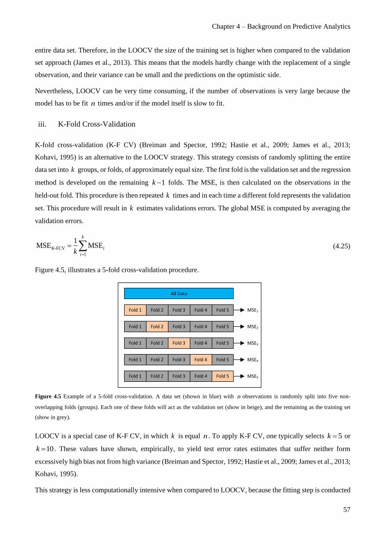
Chapter 4 – Background on Predictive Analytics
57
entire data set. Therefore, in the LOOCV the size of the training set is higher when compared to the validation
set approach (James et al., 2013). This means that the models hardly change with the replacement of a single
observation, and their variance can be small and the predictions on the optimistic side.
Nevertheless, LOOCV can be very time consuming, if the number of observations is very large because the
model has to be fit n times and/or if the model itself is slow to fit.
iii. K-Fold Cross-Validation
K-fold cross-validation (K-F CV) (Breiman and Spector, 1992; Hastie et al., 2009; James et al., 2013;
Kohavi, 1995) is an alternative to the LOOCV strategy. This strategy consists of randomly splitting the entire
data set into k groups, or folds, of approximately equal size. The first fold is the validation set and the regression
method is developed on the remaining 1k − folds. The MSE, is then calculated on the observations in the
held-out fold. This procedure is then repeated k times and in each time a different fold represents the validation
set. This procedure will result in k estimates validations errors. The global MSE is computed by averaging the
validation errors.
K-FCV
1
1MSE MSE
k
i
ik =
= (4.25)
Figure 4.5, illustrates a 5-fold cross-validation procedure.
All Data
Fold 1 Fold 2 Fold 3 Fold 4 Fold 5
Fold 1
Fold 1
Fold 1
Fold 1 Fold 5
Fold 5Fold 4
Fold 5
Fold 5
Fold 4
Fold 4
Fold 3
Fold 3
Fold 2
Fold 2
Fold 2 Fold 3
Fold 2 Fold 3
Fold 4
MSE1
MSE2
MSE3
MSE4
MSE5
Figure 4.5 Example of a 5-fold cross-validation. A data set (shown in blue) with n observations is randomly split into five non-
overlapping folds (groups). Each one of these folds will act as the validation set (show in beige), and the remaining as the training set
(show in grey).
LOOCV is a special case of K-F CV, in which k is equal n . To apply K-F CV, one typically selects 5k = or
10k = . These values have shown, empirically, to yield test error rates estimates that suffer neither form
excessively high bias not from high variance (Breiman and Spector, 1992; Hastie et al., 2009; James et al., 2013;
Kohavi, 1995).
This strategy is less computationally intensive when compared to LOOCV, because the fitting step is conducted

Part II – State-of-the-Art and Background Material
58
less times (Breiman and Spector, 1992; Hastie et al., 2009; James et al., 2013; Kohavi, 1995).
In general, cross-validation is a good approach that can be used with almost any statistical learning method.
K-F CV can be conducted in different ways: stratified sampling and repeated sampling. In stratified K-F CV
the splitting of the data into the folds involves a criterion such as ensuring that each fold has the same proportion
of observations with a given categorical value. In repeated K-F CV, the K-F CV is repeated n times, where
importantly, the split of the data is done differently at each repetition, which will result in a different training
and validation set.
iv. Comparison of LOOCV and K-F CV
LOOCV, will give approximately unbiased estimated for the test error, since each training set contains 1n−
observations, which is almost the full data set, in contrast to the validation set approach
(Breiman and Spector ,1992; Hastie et al., 2009; James et al., 2013; Kohavi, 1995).
Performing K-F CV with five or ten folds will lead to an intermediate bias level, since each training set contains
1kn
k
− observations, fewer than LOOCV, but more than in the validation set approach. Therefore, with the
goal of reducing the bias, LOOCV should be preferred to K-F CV. However, one should not only address the
bias reduction, but consider as well the procedure’s variance (James et al., 2013). LOOCV has higher variance
than the K-F CV (Breiman and Spector, 1992; Hastie et al., 2009; James et al., 2013; Kohavi, 1995). The
LOOCV method is averaging the outputs of n fitted models, and each one of them is trained on an almost
identical set of observations, and for that reason these outputs are highly correlated with each other. In contrast,
in K-F CV, the outputs of k fitted models are less correlated with each other, since the overlap between the
training sets is smaller.
The mean of many highly correlated quantities has a higher variance than the mean of many quantities that are
not as highly correlated. Therefore test error estimate resulting from LOOCV tends to have higher variance than
does the test error estimate resulting from K-F CV (Breiman and Spector, 1992; Hastie et al., 2009;
James et al., 2013; Kohavi, 1995).
4.3.2. In-sample Methods
The MSE under training conditions, is an underestimate of the MSE obtained in testing conditions. The model
is fit to the training data, using least squares, by minimizing the train MSE, but not the test MSE. Therefore, the
training error will keep decreasing as more variables are included in the model, but the test error may not follow
the same pattern. For this reason, the MSE under training conditions (or 2R ) is not a suitable parameter to select
models with different number of variables. It is not a measure of the predictive capabilities of the model, but of
its quality of fit to the data set. In order to assess the predictive accuracy of the model, it is necessary to rely on

Chapter 4 – Background on Predictive Analytics
59
some form of external validation or in out-of-sample methods, or to correct the training MSE with terms that
penalize model complexity. The later possibility will be explored in this section.
There are several methodologies that adjust the training error for the model size. These approaches can be used
to select a model from a set of models with different complexities (number of variables). Examples, of these
approaches are: Mallow’s pC , Akaike information criterion (AIC), Bayesian information criterion (BIC) and
2adjustedR . Considering a fitted least squares model containing d predictors, the Mallow’s pC estimate for the
test MSE is given by Equation (4.26) (Mallows, 1973).
( )
( )
2
1
1ˆ2
ˆwhere,
p
n
i i
i
C RSS dn
RSS y y
=
= +
= − (4.26)
RSS is the residual sum of squares, 2̂ is an estimate of the variance of the error associated with each
response measurement of the standard linear model: 0 1 1 2 2 ... m mY X X X = + + + + + .
The Mallow’s pC statistics adds a penalty term of 2ˆ2d to the training RSS to adjust for the fact that the
training error tends to underestimate the test error. The penalty term will increase as the number of predictors
increase as well, to regulate for the corresponding decrease in the training RSS (James et al., 2013). Therefore,
models with small values of test MSE tend to have small values of pC . Considering model selection, one must
select the model with the lowers pC value.
The AIC criterion (Akaike, 1974) is an Information-Theoretic parameter, and is defined for a large class of
models fit by a maximum likelihood. For a least squares model, AIC is given by Equation (4.27).
( )2
2
1ˆ2
ˆAIC RSS d
n
= + (4.27)
For least squares models, Mallow’s pC and AIC are proportional.
The BIC criterion (Schwarz, 1978), like AIC is applicable in settings where the fitting is carried out by
maximization of a log-likelihood. For a least squares model with d predictors, BIC is given by
Equation (4.28).
( ) 21ˆlogBIC RSS n d
n = +
(4.28)
BIC replaces the 2ˆ2d from Equation (4.27) by ( ) 2ˆlog n d , where n is the number of observations. Since
( )log 2n for any 7n , BIC places a heavier penalty on models with large number of variables, resulting on
the selection of smaller models than Mallow’s pC (James et al., 2013).

Part II – State-of-the-Art and Background Material
60
The adjusted 2R statistic is another common approach for selection among a set of models that contain different
number of variables. 2R is given by Equation (4.29).
2R 1RSS
TSS= − (4.29)
where RSS is the residual sum of squares and TSS is the total sum of squares.
RSS always decreases as more variables are added, and as a consequence 2adjustedR increases. For a least squares
model with d predictors, the adjusted 2R is given by Equation (4.30).
( )
( )2adjusted
/ 1R 1
/ 1
RSS n d
TSS n
− −= −
− (4.30)
In the case of 2adjustedR , a high value indicates a model with a small test error (James et al., 2013). The objective
is to minimize ( )/ 1RSS n d− − . Once all the correct variables have been added to the model, adding noise
variables will lead to a very small decrease in RSS (James et al., 2013), but will increase d and as a
consequence increase ( )/ 1RSS n d− − , eventually leading to a decrease in 2adjustedR .
All equations presented in this section for the performance metrics, are valid for a linear model estimated using
least squares. Expressions exist for more general types of models.
4.3.3. The Bias-Variance Trade-Off
As pointed out before, searching for the optimal complexity level of a regression model is an important task to
obtain a good performance. Increasing the model complexity, makes it more suitable to fit the training data,
which can lead to a decrease in the prediction error for the training data. However, the model can become highly
dependent on the training data and becomes unsuitable to predict, with good accuracy, the test data.
Figure 4.6 shows the typical behaviour of the test and training error, as function of the model complexity
(Hastie et al., 2009).

Chapter 4 – Background on Predictive Analytics
61
Figure 4.6 Test and training error as a function of model complexity (Hastie et al., 2009).
In statistical theory (Hastie et al., 2009) it is proved that the expected prediction error, also known as test or
generalization error can be decomposed as:
( )( ) ( )( ) ( )( ) ( )2
0 0 0 0ˆ ˆ ˆE y f x var f x bias f x var − = + +
(4.31)
The first term of Equation (4.31) is the variance. The variance is related to the amount by which ( )0f̂ x would
change if different training sets were used.
The second term of Equation (4.31) is the squared bias, the amount by which the average of the estimates differs
from the true mean. The bias is related to the error that is introduced by the model.
In order to minimize the expected test error, the method should simultaneously achieve a low variance and a
low bias. Both of these quantities are non-negative, therefore the expected test error can never be below
( )var , which is the irreducible error. Therefore, there is the necessity of balancing the bias and variance.
The modelling complexity is closely related to the bias-variance trade-off. More complex models tend to fit
better the training data, leading to estimates with low bias and high variance.
When a model is unable to capture the underlying pattern of the data, it is called underfitting. These models
usually have high bias and low variance. It can happen when there are a few amounts of data to build an accurate
model, or if one is trying to construct a linear model with a non-linear data.
The other scenario, is the overfitting. It happens when a model learns the detail and noise in the training data,
to such a level that has a negative impact on the performance of the model on new data.
Both overfitting and underfitting can lead to poor model performance. Overfitting, is usually, the most common
problem.
There are two important techniques that can be used when evaluating regression models to limit overfitting:
• Internal validation using out-of-sample approaches;
• External validation.

Part II – State-of-the-Art and Background Material
62
4.3.4. Performance Metrics Adopted in this Thesis
To evaluate the performance of the model it is necessary to calculate and analyse different statistical parameters.
The fundamental criterion is the prediction error or residual, ( )ˆi iy y− , which is the error between the observed
value and the predicted value of the response. In this work, it will be used the coefficient of determination
( )2R , the root mean squared error ( )RMSE and percent bias ( )PBIAS .
The values for the coefficient of determination ( )2R , for linear regression models, range from zero (the
response variable cannot be predicted by the regressors) to one (perfect match between estimated and observed
values). 2R is calculated by Equation (4.32).
( )
( )
( ) ( )
( )
( )
( )
2 2 2 2
2 1 1 1 1
2 2 2
1 1 1
ˆ ˆ ˆ
R 1
n n n n
i i i i i i
i i i i
n n n
i i i
i i i
y y y y y y y y
y y y y y y
= = = =
= = =
− − − − −
= = = −
− − −
(4.32)
where iy is the thi observed response, ˆiy is the corresponding estimate, y is the mean of y , ( )
2
1
n
i
i
y y=
− is
the observed variability, ( )2
1
ˆ
n
i
i
y y=
− is the variability explain by the regression and ( )2
1
ˆ
n
i i
i
y y=
− is the
variability not explained by the model (residual variation).
The 2R statistic has the interpretation as the proportion of variation of Y which is explained by the last squares
prediction function due to the following decomposition:
( ) ( ) ( )2 2 2
1 1 1
ˆ ˆ
Total Variation = Explained Variation + Unexplained Variation
n n n
i i i i
i i i
y y y y y y= = =
− = − + − (4.33)
For non-linear methods, the coefficient of determination needs to be considered with strong limitations, because
the ANOVA decomposition does not hold in general for non-linear models. The 2R statistic defined in
Equation (4.32) is not applicable to a nonlinear model, since the decomposition in Equation (4.33) no longer
holds. Therefore, for such cases it needs to be considered as a parameter loosely associated with model quality
(but does not necessarily has to lie between 0 and 1).
The root mean squared error ( )RMSE is a common measure of accuracy to estimate the standard error of
prediction obtained for the model and is given by Equation (4.34). The lower its value, the better the prediction
performance of the corresponding method.

Chapter 4 – Background on Predictive Analytics
63
( )2
1
ˆ
RMSE
n
i i
i
y y
n
=
−
=
(4.34)
where iy is the thi observed response, ˆiy is the corresponding estimate, and n stands for the number of
observations in the testing set.
The percent bias ( )PBIAS measures the average tendency of the estimated values to be larger or smaller than
the observed responses. The optimal value for PBIAS is zero, with low-magnitude values indicating accurate
model estimation. Positive values indicate overestimation bias, whereas negative values indicate
underestimation bias. PBIAS is given by Equation (4.35).
( )
( )
1
1
ˆ
PBIAS 100
n
i i
i
n
i
i
y y
y
=
=
−
=
(4.35)

64
This page was intentionally left in blank

65
Part III ‒ Methods and Data Sets
“If you torture the data long enough, it will confess”
Ronald Coase

66
This page was intentionally left in blank

67
Chapter 5. A Pipeline for Inferential Model Development
As mentioned in Section 4.1, four stages were identified that are usually part of a pipeline for the development
of inferential sensors: acquisition of data and process knowledge; data analysis; model estimation; and model
validation. In the end, the final workflow to be adopted should be chosen according the specific goal, industrial
process and data available. Equation Chapter (Next) Section 1
The main components of the data analysis pipeline for inferential model development used in this thesis are
summarized in Figure 5.1 and will be described in more detail in the following sections.
Figure 5.1 Data analysis pipeline for inferential model development adopted in this thesis.
The initial step of data analysis is related to data acquisition. Good quality data are needed to develop a
data-driven model and an appropriate initial overview of the data and process is fundamental to understand the
data structure and relationships with the process units they are collected from.
Data cleaning concerns the activities of detecting and removing possible outliers, as well as identifying periods
of time when the plant was not undergoing normal operating conditions. A more detail description of this stage
is presented in Section 5.2.
In the pre-processing stage, one should define the resolution of data analysis. Process variables are stored every
minute, while RON measurements are performed once per day. Since we are dealing with a real industrial case
study, missing values will also occur and need to be accounted for. Therefore, setting the proper time resolution
is an important decision that needs to be made. It secures that all data have the same resolution and share similar
meanings in terms of the windows of time they refer to. Empty slots of data need to be filled using missing data
imputation mechanisms. The selection of the resolution and missing data imputation techniques used in this
stage are described in Section 5.3.
After conducting these three steps, a processed data set is obtained and will be used for model building purposes.
The framework developed to assess and compare all the estimation methods considered in this work, and the
associated ranking system, are presented in Section 5.4.

Part III – Methods and Data Sets
68
5.1. Data Acquisition and Inspection
All data was initially transferred to Microsoft® Excel using Visual Basic for Applications (VBA) code. The
subsequent analysis was carried out in the MATLAB® environment (The MathWorks, Inc.)
In this work, two different units were studied: SRR and CCR. For both cases, the information collected, did
come from two major sources: process variables and product quality variable. Process variables are related to
the operation and contain measurements of flow rates (e.g., feed and hydrogen), temperatures (e.g., feed,
reactors, and columns) and pressures (e.g., reactors, columns and recycled hydrogen). The product quality
variable, RON, is the target response variable. It is obtained from the laboratory, following a standard procedure,
which corresponds to the ASTM Method D-2699.
These two types of variables have distinct sampling rates. Process variables are collected every minute, whereas
RON is measured once each day (or less). Therefore, the industrial data set has a sparse, multirate structure, and
also include outliers, as well as missing data (due to problems in data transmission, process shutdowns, etc.).
These aspects were considered and handled in the analysis workflow, namely during the stages of data cleaning
and pre-processing. For real industrial settings, such stages are critical and should never be underestimated,
since lots of resources and time need to be allocated before being able to come up with a good quality final data
set, from which useful knowledge can be then extracted through appropriate process mining tools.
To evaluate possible problems related with outliers, a simple time series plot for all variables was performed,
in order to identify the presence of Global and Contextual outliers. Alongside process engineers, it was also
possible to identify the presence of maintenance and shutdown periods.
The results of this analysis are presented in Section 7.1.1 (SRR unit) and Section 7.2.1 (CCR unit).
5.2. Data Cleaning
In the case of data collected from Chemical Processing Industries, one has to handle with several issues related
to data quality and structure, such as: presence of outliers and noise, missing data, multiple sampling rates
(multirate), multiple resolutions (multi-resolution or multi-granularity), high dimensionality, strong
correlations, etc.
In this work, the data cleaning stage is mostly focused on detecting outliers and eliminating periods where the
process was not operating or data is of poor quality. The data cleaning stage includes the identification and
processing of periods of operation and non-operation (e.g., maintenance). Periods of non-operation should be
identified and removed from the analysis. This procedure was mostly based on information provided by the
plant engineers and process knowledge. As for the periods of operation, the focus was on detecting outliers.
Global outliers were identified with success by applying simple variable-dependent thresholds, called operation

Chapter 5 – A Pipeline for Inferential Model Development
69
limits. Since each process variable has its own operating range, any value beyond that limit was considered an
error. The periods when a given variable had its values outside the operating range were not removed from the
analysis, but replaced with “blanks”, i.e., turned into missing values since they do not represent the normal
operating range of each variable. The limit operating ranges for each variable were also provided by the plant
process engineers.
Contextual outliers are more difficult to identify, because they are consistent with the technical operation ranges
and the physical limits of the sensors, but significantly deviate from the local behaviour or the local pattern of
dispersion expected for the values of certain variables. Several techniques were applied to identify these
contextual outliers, such as the 3 rule, the Hampel identifier (Fortuna et al., 2007; Scheffer, 2002;
Souza et al., 2016)(Fortuna et al., 2007; Scheffer, 2002; Souza et al., 2016)and the modified Hampel identifier
with a moving window technique (Fortuna et al., 2007; Scheffer, 2002; Souza et al., 2016). For the moving
window technique, the window size was adapted for each variable, by selecting among a list of possible
consecutive values {50; 500; 1,000; 2,000; 3,000; 5,000} . The selection of the most adequate window size was
done by visual inspection of the data, alongside with the opinion of plant engineers, in order to confirm that the
points that were removed were indeed outliers and were not representative of the process operation. This visual
and expert-supervised confirmation is of extreme importance to assure an adequate cleaning stage and that
useful information is not thrown away together with inadequate data.
The results of this step are presented in Section 7.1.2 (SRR unit) and Section 7.2.2 (CCR unit).
5.3. Data Pre-Processing
In the pre-processing stage, some structural aspects of the cleaned data set are fixed in order to make it ready
for further analysis. The main aspect to handle here, is the multirate nature of the data set. Another relevant
topic of interest is related to missing measurements caused by transmission problems and other sensor/process
malfunctions, which also contribute to the sparsity of the data set. These aspects are covered in the
pre-processing stage, which includes two tasks: (i) selection of the time resolution for conducting the analysis;
(ii) missing data imputation.
5.3.1. Resolution Selection
As stated above, both data sets (SRR and CCR) have several process variables (collected every minute) and
response variable (collected, at best, once per day). This mismatch in acquisition rates and sampling times,
limits the amount of dynamic information that is possible to infer from data (according to the Nyquist theorem)
and generates a sparse data structure that raises many problems for model building, as the observations where
regressors are available do not coincide with those where the response is known.

Part III – Methods and Data Sets
70
The two sets of variables carry information with different levels of detail about the process, and therefore, it is
necessary to first establish a common resolution level for both process and quality variables.
Resolution is characterized as the length of the non-overlapping time windows over which measurements are
aggregated by computing some summary statistic (e.g., mean, median, etc.). The resolution level should be
selected taking into account the goal of the process analysis and the structure of data. The objective is to develop
a predictive model for the estimation of RON.
It is necessary to select a resolution level, which means that process and laboratory quality measurements will
be aggregated at the same resolution level and saved for further analysis. This procedure not only bring all
variables to a common resolution level, but also reduces the data set volume and minimizes the multirate sparsity
present in the raw data. The operator used for the aggregation was the median. The median was used instead of
the mean, given its better properties of robustness to the presence of outliers, which is a useful feature when
quickly analysing large amounts of industrial data.
In this work, three different resolution-oriented analysis were studied: (i) unsynchronized single resolution with
time support of twenty-four hours (U-SR24); (ii) synchronized single resolution with time support st
(S-SR st ); (iii) synchronized single resolution with time support of one hour and a lag level of two (S-SR1L2).
For U-SR24, a time support of twenty-four hours was selected, which means that process and laboratory
measurements from one day were aggregated and saved for further analysis. This procedure helped to minimize
the level of the sparsity of raw data, which reduces the number of missing values and the data set volume. The
aggregation of the data for each day considers the median of each variable for each day in question. The
pseudo-code of this approach is presented in Appendix A.1, Table A.1 (page 139).
For the S-SR st scenario, the aggregation was based on the time occurrence of the output variable with a time
support value of st . If RON occurs at time period RONt , the aggregation of the data is performed between
( )RON st t− and RONt (i.e., it is synchronized with the response). Once again, the aggregation of the data
considers the median value for each variable during the time period in question. For this class, several time
support values were considered: twenty-four (S-SR24); four (S-SR4); three (S-SR3); two (S-SR2); one hour
(S-SR1). The pseudo-code for these four scenarios is presented in Appendix A.2, Table A.2 (page 140).
Figure 5.3 describes the example of the scenario S-SR3. Since the time support is equal to three, all the
aggregations windows are between ( )RON 3t − and RONt .

Chapter 5 – A Pipeline for Inferential Model Development
71
X1 X2 YX3
tim
e su
pp
ort
= 3
tim
e su
pp
ort
= 3
(a)
Figure 5.2 Representation of the S-SR st methodology with a time support of three hours.
Taking into consideration the example illustrated in Figure 5.2, the data set resulting from the S-SR3
methodology has only two observations, because there are only two available values for Y. The first aggregation
period takes place between 2t and 5t , and the second, between 7t and 10t . Independently of the size of the time
support, the resulting data set has always the same number of observations, because it is constructed based on
the amount of RON’s observations.
Finally, for S-SR1L2, it was intended to reduce the time support value for one hour but introducing a new
dynamic modelling concept, the lag. The lag corresponds to a translation to the past imposed on a variable,
given as a multiple of the time support adopted. The time support defines the resolution, whereas the lag is used
to account for process dynamics and does not change the variables resolution. For S-SR1L2, three different lag
levels were studied: zero, one and two. The pseudo-code for this scenario is presented in Appendix A.3,
Table A.3 (page 141). Since the resolution is equal to one, the effective aggregations windows are between
( )RON s st lag t t− − and ( )RON st lag t− , as shown in Figure 5.3. The left side of Figure 5.3 represents the
lag of zero, at the centre the lag of one hour and on the right side the lag of two hours.

Part III – Methods and Data Sets
72
X1 X2 YX3
lag = 0
lag = 0
X1 X2 YX3
lag = 1
lag = 1
X1 X2 YX3
lag = 2
lag = 2
(a)
time
t1
t2
t3
t4
t5
t6
t7
t8
t10
t9
(b) (c)
Figure 5.3 Schematic representation of the S-SR1L2 methodology with a time support of one hour with: (a) lag of 0; (b) lag of 1;
(c) lag of 2.
For all the lags, the length of the aggregation window (time support) is one hour. For this example, the data after
applying S-SR1L2 is composed by the original set of predictors plus its two time-shifted versions (designated
by Figure 5.3b and Figure 5.3c). In general, the original set of K predictors is extended with ( )K m additional
time-shifted predictors (on top of the original set of predictors), where m stands for the number of different lags
studied (in this case 3).
Taking into consideration the example provided in Figure 5.3, after applying the S-SR1L2 scenario, the resulting
data set would have only two observations, because there are only two available values for Y. For lag level zero,
the first aggregation is between 4t and 5t , and the second aggregation between 9t and 10t . For the lag level of
one, the aggregations are between 3t and 4t , and 8t and 9t . Finally, for the lag level of two, the aggregations
are between 2t and 3t , and 7t and 8t .
5.3.2. Missing Data Imputation
There are several reasons for the existence of missing values in the data set (besides the multirate issue discussed
above). The most prevalent are related with: (i) maintenance periods of time; (ii) occasional failures and physical
malfunctions of the sensors (since sensors are electro-mechanical devices, they may undergo sporadic failure
conditions); (iii) transmission errors from the sensor to the receiver or across the IT system before reaching the
database. While the periods covered in (i) were removed from the analysis, the periods in (ii) and (iii) need to
be handled through data imputation schemes.
Missing data techniques estimate sequences of missing information by exploiting associations between variables
(cross-correlation) or in time (autocorrelation). Various methods were developed to take advantage of the

Chapter 5 – A Pipeline for Inferential Model Development
73
existence of cross-correlations, under missing at random (MAR) and missing completely at random (MCAR)
scenarios, some of them based on the expectation-maximization (EM) approach (Arteaga and Ferrer, 2002;
Little and Rubin, 2002; Nelson et al., 1996; Walczak and Massart, 2001a, 2001b). In both case studies, there is
a large process unit with massive inertial elements and high characteristic dynamic time constants. At the same
time, data is being collected at very fast acquisition rates (every minute). These two conditions together generate
strong autocorrelation patterns. Autocorrelation represents the degree of similarity between a given time series
and a lagged (e.g., delayed in time) version of itself over successive time intervals. Given measurements,
1 2, , ..., NY Y Y at times 1 2, , ..., Nt t t , the autocorrelation function, at lag k , is defined by Equation (5.1).
( )( )
( )
1
2
1
N k
i i k
ik N
i
i
Y Y Y Y
r
Y Y
−
+
=
=
− −
=
−
(5.1)
Autocorrelation is a correlation coefficient of a variable with itself shifted in time by a certain time lag. A data
trend has a strong autocorrelated behaviour when autocorrelation coefficients are large for some lag (especially
for lag 1). If the dominating association structure present in the data set corresponds to variable’s
autocorrelations, it is possible to use interpolative schemes to estimate missing data. For example, the imputation
can be performed by a moving window technique, where missing data at the centre is replaced by the median
of the data points falling within the moving window.
In Section 7.1.3 (SRR data set) and 7.2.3 (CCR data set), are presented the results and justification for selecting
the interpolative methodology as the missing data imputation scheme.
5.4. Data Modelling
During the design of an inferential model, it is of extreme importance to select the most appropriate modelling
strategy. However, it is not possible to make such selection a priori, neither is it recommendable to adopt the
methods the user is most familiar with, or that were successfully applied in other unrelated applications. The
strategy followed in this work is to comprehensively study the prediction ability of a wide variety of
methodologies and compare their performance in the current case (data set). A brief description of the methods
considered in this work were presented in Section 4.2. This section describes how the pool of methods were
compared. Reference is also made to additional insights that can be extracted from the models estimated.
5.4.1. Model Comparison Framework
In the proposed pipeline, the set of predictive models were compared through a protocol that combines Monte
Carlo Double Cross-Validation (Geisser and Eddy, 1979; Krzanowski, 1982; Rendall and Reis, 2018;

Part III – Methods and Data Sets
74
Stone, 1974; Wold, 1978, 1976) for robust estimation of the methods’ hyperparameter(s) and for prediction;
statistical hypothesis to rigorously assess the methods’ relative performances; and finally scoring operation, to
summarize the results of the pairwise comparison tests in an easily interpretable ranking of their performance.
It is important to mention that no method from the classes referred above is expected to perform always better
than the others and claim overall predictive superiority. Therefore, the final decision about which method to use
should be based on a rigorous consideration of the options available. When the choice is not obvious, the
decision process benefits from a robust comparative analysis. Thus, a state-of-the-art comparison methodology
based on Monte Carlo Double Cross-Validation was implemented in order to establish rankings of the best
methods to adopt for addressing a particular problem, like the one being handled here.
The methodology described in Table 5.1, starts by defining the number of Monte Carlo runs to be conducted
( )MCn in the outer cycle of the framework, i.e., the number of times the internal operations will be repeated.
The internal operations consist of randomly splitting the data set into a training and testing set (step 1.a). The
training set is then used to select hyperparameter(s) using a 10-fold cross validation (step 1.b) and a model is
built using the training set (step 1.c) predict the test set and save the prediction errors (step 1.d). The
hyperparameter(s) for each method and more details on how they were optimized in step 1.c can be found in
Appendix B, Table B.1 (page 142). For this work, each data set (SRR and CCR) for each resolution scenario,
MCn was defined as 25.
Concerning the pseudo-code presented in Table 5.1, there is the need to discuss two aspects about the splitting
(step 1.a) and the tuning of the hyperparameter(s) (step 1.b).
For the splitting of the data, described in step 1.a, the 80/20 ratio was established. The splitting of data can occur
in three ways: (i) order split; (ii) random split; (iii) random stratified sampling split. In the case of order split,
the first 80% samples go to the training set and the remaining ones to the testing set. The problem with this
strategy is that it does not, always, provide a balanced representation of all the conditions where the model
should be trained. Therefore, in this work we have adopted the random stratified sampling split, which consists
of splitting the response variable into a pre-selected number of intervals based on its percentiles (e.g., 0-25th,
25th-50th, 50th-75th and 75th-100th percentiles). From each group, 80% of the data will be randomly selected to
form the training set, and the rest goes to the testing set.
The training set is then used to optimize the selection of the hyperparameter(s) of each model. Since in some
industrial processes it may be difficult to obtain sufficient historical data to develop a model, it is advantageous
to use the K-fold cross-validation technique (K-F CV). As a rule of thumb, 10 folds were used for the 10-fold
cross-validation (step 1.b). From the existing ten folds, nine are retained to train a model, and the remaining
fold is used to perform a cross-validation. This process is repeated ten times, ensuring that each fold is used
once and only once, in the validation process. This 10-fold cross-validation is repeated ten times, representing
the inner cycle of (step 1.b). The RMSE in the left-out fold, obtained for each possible value of the
hyperparameter(s), is saved and the one leading to the lowest RMSE value is adopted for model development

Chapter 5 – A Pipeline for Inferential Model Development
75
process.
The prediction errors are calculated with the root mean squared error for the testing set ( )testRMSE , given by
Equation (4.34), and another metric to evaluate the prediction capability of regression methods is the ( )2testR ,
the coefficient of determination for the test set, calculated according to Equation (4.32).
Since the outer cycle can be performed multiple times, it is possible to characterize the individual performance
of the methods through their distributions of testRMSE (lower values suggest better predictive performances).
In each run, the training and testing data sets for all the methods, under comparison, are exactly the same.
Therefore, it is possible to compare different methods by accessing the statistical differences found in the
prediction errors between them. This comparison is performed through paired t -tests (given the high number
of runs, the Central Limit Theorem assures a convergence of the mean to a Gaussian distribution, which justifies
the adoption of this test). The null-hypothesis states that the mean difference between two methods under
comparison is zero (i.e., the means of testRMSE for the two methods is equal). The null-hypothesis is rejected
whenever the p-value obtained is lower than the adopted significance level (in this case, the significance level
was set to 0.05 = ). To facilitate the analysis of the relative performance of the methods resulting from the
battery of pairwise statistical tests, a scoring system was implemented. For each pair of methods under
comparison a score of 1 (“wins”) is given to the method with statistically significant lower testRMSE (e.g.,
better prediction performance). A score of 0 (“loss”) is given to the method with statistically significant higher
testRMSE (e.g., worse prediction performance). In case the prediction performance of the two methods is not
statistically distinct, a “draw” has occurred.
If a “draw” occurs, it is not clear which score should be attributed, and any value in the interval ]0,1[ could be
arbitrarily chosen. By specifying a value in this interval, the performance of each method is obtained from the
sum of the scores obtained in all pairwise comparisons, which would be a reasonable Key Performance Indicator
(KPI). However, as this sum depends on the actual score attributed to the “draws”, and any specific value would
be debatable, we have computed the average KPI for all possible weights on the interval ]0,1[ . More
specifically, we have calculated two KPIs for the relative performance of each method: the mean KPI and the
mean RANK, defined as follows:
• Mean KPI – the average of the sum of scores when the “draw” scores span the interval ]0,1[
( ) ( )1 1
0 0
1KPI
1 0m m mKPI s ds KPI s ds= =
− (5.2)
• Mean RANK – the average rank (in the descending ordering of performance) obtained when the “draw”
scores span the interval ]0,1[

Part III – Methods and Data Sets
76
( ) ( )1 1
0 0
1RANK
1 0m m mRANK s ds RANK s ds= =
− (5.3)
Table 5.1 Pseudo-code for the comparison framework.
1. For i=1: MCn (number of outer cycles) perform:
a. Randomly split the complete data set into a training (80%) and testing set (20%);
b. The training set is used to tune the hyperparameter(s) using 10-fold cross-validation (inner cycle).
c. Estimate the model with the training set and the selected hyper-parameter(s);
d. Predict the observation in test set and compute the Root Mean Squared Error (testi,RMSE m , where m is the index of the method
in course).
2. Apply a paired t -test to assess the statistical significance of the difference between the MC
test1:N ,RMSE m for all pairs of methods.
3. Using the p-values for paired statistical tests compute the overall performance criteria:
a. Compute KPIm using Equation (5.2);
b. Compute Rankm using Equation (5.3).
In the implementation of this methodology, variable auto-scaling (or z-score transformation using the mean and
standard deviation of the training set) was applied in each run of the outer cycle, to avoid any bias in the
estimation of the testing set.
It is important to mention that for the unsynchronized scenarios, since the size of the data set is bigger when
compared with the synchronized scenarios, the values of the response vector in the test conditions used in the
computations correspond only to observed values and not imputed values. In this way, the testRMSE obtained
by the different approaches is realistic and comparable.
5.4.2. Analysis of Variable’s Importance
The analysis of variables’ importance may bring additional insights about the problem under analysis. The
approaches developed in this work are based on the analysis of the regression vectors obtained with the several
linear regression methods contemplated in this study. The rational is that variables’ importance mainly concerns
the relevance of the main effects in a regression model which correspond to the linear terms, and these terms
are well estimated by linear frameworks. However, alternative methods do exist, such as the Random Forests
built-in feature for assessing variables, briefly referred in the end of this section.
The importance of variable i according to the method j is related to the magnitude of the corresponding
regression coefficient, ,i j (note that data was autoscaled, and therefore the magnitude of the coefficients
reflects the importance of the respective variables, independently of their original units and scales of
measurement). Since there are k outer cycles (Monte Carlo simulations) the cumulative score, ,i jB , for each
variable and method is calculated by Equation (5.4):

Chapter 5 – A Pipeline for Inferential Model Development
77
( ), ,
1
ˆouter cyclen
ki j i j
k
B −
=
= (5.4)
The relative normalized importance of a variable for a specific method is computed by Equation (5.5). This
expression assigns values between 0 and 1 to each variable. A relative importance of 0 means that the variable
is least important for a respective method, while a relative importance of 1 corresponds to the most important
variable for that particular method.
( ) ,
,
i j
R i j
BI X
−=
−
MinB
MaxB MinB (5.5)
where ( ),R i jI X stands for the relative importance of variable i for method j ; ,min i ji
B=MinB and
,max i ji
B=MaxB , representing the minimum and maximum in the set of all ,i jB for method j , respectively.
The relative importance of a variable under the scope of a given method, as defined by (5.5), can be used to
derive an overall assessment of variable importance under the global scope of all the methods under analysis.
The procedure adopted consist of computed a weighted average of the relative importance for method j ,
weighted by some function of the quality of the respective model. In fact, since some methods perform better
in predicting the response than others, this fact was taken into account and methods with better performance are
given more credibility in their assessment of the variables’ importance. The weight for method j is given by
2test,norm jR , which is the coefficient of determination under test conditions, 2
testR , after normalization to fall
under the range between 0 and 1. Normalizing 2testR will ensure that the best method will contribute to the global
importance with a weight of 1, while the worst method will do so with a weight of 0. The normalized coefficients
of determination are computed via Equation (5.6).
2test,2
test,normj
j
RR
−=
−
2test
2 2test test
minR
maxR minR (5.6)
where 2test, jR is the coefficient of determination for testing conditions of method j , the term
2,max test jR=2
testmaxR and 2,min test jR=2
testminR represent the maximum and minimum values of 2test, jR .
The global importance of each independent variable is then assessed by applying Equation (5.7).
( )
( )methods
2, test,
1
methods
norm
n
R i j j
j
G i
I X R
I Xn
=
=
(5.7)
where ( )G iI X is the global importance for variable i , 2test,norm jR is the
2test, jR normalized for method j and
methodsn stands for the number of methods considered for this methodology.

Part III – Methods and Data Sets
78
As mentioned above, alternative variables’ importance metrics are also available, such as PLS VIPs and
approaches built over the outcomes of Random Forests, for instance using the out-of-bag (OOB) permuted
predictor errors. If a predictor that is important for the model, permuting its values should affect the model error.
If a predictor is not influential, then permuting its values should have little or no effect on the model error. These
observations leads to the concept of permutation importance (Breiman, 2001). It is defined as the mean increase,
over all the trees in the forest, of the out-of-bag error of a tree obtained when randomly permuting the variables
in the OOB samples. In random forests for model regression, the OOB error of a tree is measured by the mean
squared error (MSE). In summary, the greater the error increase, the more important the variable is. This metric
was also applied in this thesis, using the built-in function provided by Matlab called OOB permuted predictor
delta error.

79
Chapter 6. Data Sets Collected from the SRR and CCR Units
This chapter provides a brief overview regarding the raw data sets used in this thesis. Two data sets were
analysed, one collected from the semi-regenerative catalytic reformer (SRR) and another from the continuous
catalytic reformer (CCR). Both industrial units are located at the Matosinhos site of Galp.
6.1. Semi-Regenerative Catalytic Reformer (SRR) data set
The SRR data set was obtained from the SRR unit of the fuels plant at Matosinhos refinery. The data set contains
969,120 samples, spanning a period of 21 months. It contains process variables from the catalytic reforming
unit, as well as product quality data concerning the target response variable, RON. Data collected form the
process includes measurements of flow rates (e.g., feed and hydrogen), temperatures (e.g., feed, reactors, and
columns) and pressures (e.g., reactors, columns and hydrogen). These process variables are collected every
minute.
The product quality variable is the response variable, RON, which is measured in the laboratory following a
standard procedure, ASTM Method D2699. Although the sampling rate of RON is different from that of process
variables, it is possible to identify when the sample was collected.
A total of forty-one process variables were employed in this study for predicting RON.
6.2. Continuous Catalytic Reformer (CCR) data set
The CCR data set was obtained from the CCR unit of the fuels plant at the Matosinhos refinery. The data set
contains 1,048,320 samples, spanning the period of 24 months. The information regarding the CCR is from two
sources: process variables and product quality variable. The process variables are related to the operation and
consist of similar measurements as in SRR. The process variables for the CCR data are also collected every
minute.
The product quality variable is the response variable, RON, which is measured in the laboratory following the
same standard procedure, ASTM Method D2699. The RON measurements collected from the CCR unit show
different sampling rates when compared to the process variables.
A total of forty-one process variables were employed in this study for predicting RON.

80
This page was intentionally left in blank

81
Part IV ‒ Results and Discussion
“The goal is to turn data into information and information into insight”
Carly Fiorina

82
This page was intentionally left in blank

83
Chapter 7. RON Prediction from Process Data: Results
In this chapter the results obtained for every step of the data analysis pipeline for inferential model development
described in Chapter 5, are presented. The analysis outcomes are presented for each data set (SRR, CCR),
including data cleaning, all pre-processing steps, and the predictive assessment for all regression methods
considered. Finally, we address the selection of the analysis resolution and the incorporation of dynamical
elements in the inferential model, for both units.
7.1. Results for the SRR unit
As discussed before, it is important to perform a first analysis on the data in order to identify the presence of
possible outliers, missing data and the variability of the RON. The SRR data set is composed by 969,120 samples
for 41 process variables, covering a period of 21 months. Table 7.1 presents the number of measurements
available of RON for the SRR data set, as well as the corresponding range of values.
Table 7.1 Number of RON samples and the corresponding range, mean and standard deviation.
Property Number of samples Property values
Min. Max. Mean SD
RON 173 75.60 101.00 96.96 2.62
7.1.1. Data Acquisition and Inspection
After data collection, it was possible to identify that the SRR data has a multirate structure: process variables
are collected every minute and RON, which is the quality variable, is collected at best once per day. Each
measured value is the instantaneous measurement and it is possible to have access to the collection time.
Figure 7.1 gives an overview of the time series of RON and the example of a process variable 1X (process
variables are anonymized for protecting critical industrial information).

Part IV ‒ Results and Discussion
84
Figure 7.1 (a) Time series plot of RON during the data collection period; (b) Time series plot of 1X during the data collection period.
Analysing Figure 7.1a and Figure 7.1b, is it possible to identify three zones highlighted by the red dash lines
that need to be further investigated and possibly excluded. For Figure 7.1b on the left side, it is possible to verify
the existence of values that are outside the normal distribution of data. The regions at the middle and right,
correspond to time periods where no data was collected. All of these three periods were classified as
non-operation periods due to shutdowns or maintenance interventions. The identification of these three zones,
was only possible due to information provided by process engineers.
As seen by Figure 7.1b, outliers are present in the data set. The following section provides the results of the data
cleaning step, which is the second step of the data analysis workflow proposed in Chapter 5.
Figure 7.2 gives an overview on the level of missing data present in the data set after the data collection step.
Figure 7.2 Comparison of the percentage of missing data present in the collected data.
For variable 1X , there are 79,919 missing entries out of the 969,120 samples (8.25%). Most of these missing
records fall in the red regions identified in Figure 7.1.
(a) (b)

Chapter 7 – RON Prediction from Process Data: Results
85
7.1.2. Data Cleaning
As described before, several data cleaning filters were conducted over the data set with the objective of
identifying and removing periods of operation and non-operation (e.g., shutdown or maintenance). For
illustration purposes, Figure 7.3 presents the results obtained in the cleaning stage of the data analysis workflow
for variable 1X . Figure 7.3a illustrates the data distribution for process variable 1X . As verified in the previous
section, the red dashed lines identify time periods corresponding to non-operation, which were therefore
removed from the analysis. The black line represents the collected data.
Abnormal values can be identified by applying an operation filter. These abnormal values are called Global
outliers. Each process variable has its own operating range and Figure 7.3b presents the case of variable 1X
after this stage is conducted (blue line). From the blue line of Figure 7.3b it is possible to observe that there are
still data points left to be removed. These points, as mentioned above, are classified as Contextual outliers.
To remove the contextual outliers, three strategies were tested: 3 rule, the Hampel identifier and the modified
Hampel identifier with moving window technique.
From Figure 7.3c it is possible to verify that the upper and lower thresholds obtained from the 3 rule do not
identify most of the data points considered to be contextual outliers. The Hampel identifier in Figure 7.3d leads
to similar results as the 3 rule, failing to detect and remove most of the data points considered as outliers.
Both of these procedures were unable to detect a large fraction of the existing outliers, since their thresholds are
influenced by the existence of outliers, leading to inflated “normal” intervals.
(a) (b)

Part IV ‒ Results and Discussion
86
Figure 7.3 Comparison of various cleaning steps over the same variable 1X : (a) No cleaning filter; (b) Operation filter; (c) 3 filter;
(d) Hampel Identifier; (e) adaptive Hampel identifier with moving window technique. The black line for (c), (d) and (e) represent the
same, they represent the blue line from (b).
The Hampel identifier with moving window is a better alternative, since it does not consider the data set as a
whole, but only the local variability for defining the filtering thresholds. A window size was selected for each
variable from a list of possible sizes 50; 500; 1,000; 2,000; 3,000; 5,000 . The selection of the most adequate
window size was done by visual inspection of the data, alongside with the opinion of plant engineers, in order
to confirm that the points removed were indeed outliers and were not representative of real process operation.
From Figure 7.3e it is possible to observe that most of the outliers were identified as such and therefore removed
from the data set. The adaptive Hampel algorithm was applied to all the remaining process variables.
7.1.3. Data Pre-processing
This section provides the results of the different resolution scenarios described in Section 5.3 (page 69).
Table 7.2 illustrates the number of samples present in the data set for each resolution scenario, as well as the
level of missing data at each resolution (for illustration purposes results are only provided for variable 1X ).
(c)
(e)
(d)

Chapter 7 – RON Prediction from Process Data: Results
87
Table 7.2 Number of samples and respective percentage of missing data for each resolution studied.
Resolution Scenario Number of samples Number of predictors Missing data 1X (%)
Collected Data 969,120 41 8.25
Data Cleaning 753,120 41 2.87
U-SR24 523 41 1.34
S-SR24 150 41 0.00
S-SR4 150 41 0.00
S-SR3 150 41 0.00
S-SR2 150 41 0.00
S-SR1 150 41 0.00
S-SR1L2 150 123 -
The “Collected Data” refers to the original data set, after the data collection stage. After the data cleaning stage,
since the removal of the non-operation periods was conducted, the number of samples was reduced. The
non-operation period represents 216,000 samples out of 969,120. Therefore, the data set after the data cleaning
stage is composed by 753,120 samples. From the remaining 753,120 samples, there is still missing data present,
since the global and contextual outliers were replaced by blanks and not removed from the data set.
For the unsynchronized scenario (U-SR24), the data set has 523 new observations corresponding to the medians
of the aggregation periods. For the U-SR24 each observation represents one day of operation. After this
procedure, variable 1X still has seven missing records out of 523, and such an issue needs to be handled through
missing data imputation.
For the synchronized scenarios, the data set is composed by 150 new observations, because there are only 150
measurements of RON present in the data set. This value is smaller than the one presented in Table 7.1 (173),
because in the data cleaning stage 23 observations of RON were removed. After these scenarios, variable 1X
does not have missing records, but other variables may have, and this issue needs to be handled.
While the unsynchronized single resolution and all synchronized single resolution with no lags, consider 41
predictors, the S-SR1L2, has three times more predictors, because three different lags were studied at the same
time ( )lag = 0, 1, 2 . Once again missing data can occur, so missing data techniques need to be applied.
As mentioned above, both unsynchronized and synchronized methodologies reduce the volume of data in terms
of observations.
In practice, the percentage of missing data, for the synchronized single resolution scenario, decreases with the
increase of the time support. The observations present in the window with the size of one hour are also included
in windows of size three hours (Figure 5.2, page 71); missing data relative to a time support of one hour will
also be present in larger time windows, possibly along with other non-missing observations. Therefore, selecting
a coarser data resolution mitigates the existence of missing data.

Part IV ‒ Results and Discussion
88
Figure 7.4, provides an illustration on how the level of missing data changes for the different single resolution
scenarios studied.
Figure 7.4 Comparison of the percentage of missing data, for all variables, before and after the selection of the resolution.
Despite this fact, some empty records may still remain as can be observed in Table 7.2 and Figure 7.4. Thus,
missing data imputation techniques are required to handle these cases. For example, variable 1X , for the
scenario U-SR24, has seven missing records out of 523 (1.34% of missing data), but when using a synchronized
methodology, that value becomes zero.
Data imputation exploits some type of potential redundancy in the data: either variables’ mutual correlation,
autocorrelation or both. Figure 7.5, presents the autocorrelation for variable 1X , and its correlation with other
variables, where it is clear the strong autocorrelation for small lags.
Figure 7.5 (a) Autocorrelation function for variable 1X for the U-SR24 scenario; (b) Pearson correlation between 1X and the other
process variables for the U-SR24 scenario.
When data have a trend, the autocorrelation for small lags tend to be large and positive because observations
nearby in time are also closely associated. The correlation of 1X and the rest of the variables in Figure 7.5b is
not as strong as the autocorrelation (note that the value of 1 concerns the correlation of 1X with itself).
(a) (b)

Chapter 7 – RON Prediction from Process Data: Results
89
Therefore, as the dominating correlation structure in the SRR data set corresponds to variable’s autocorrelation,
it was adopted a robust interpolative method to estimate missing records for each scenario. More specifically,
the imputation was performed via a moving window median approach.
In this work, the missing data imputation problem was addressed by taking advantage of the variable
autocorrelation. Nevertheless, EM methods could also be used to exploit the correlation and autocorrelation.
However, the interpolative method is simpler, computationally more scalable and showed satisfactory accuracy,
and was therefore adopted.
7.1.4. Predictive Accuracy Assessment
In this section, the results of the Monte Carlo Double Cross-Validation are presented, based on which the
performance of the different regression methods is assessed and compared.
The average values of the performance metrics obtained for all the test sets during the Monte Carlo Double
Cross-Validation procedure are presented from Table 7.3 to Table 7.7. The results for all methods for the
different resolution scenarios, concerning testRMSE , 2testR and testPBIAS , are presented in the next subsections.
i. U-SR24 Scenario
Table 7.3 provides the performance indexes of all the regression methods for the unsynchronized single
resolution scenario U-SR24. For this case, the data set has 523 samples and 41 predictors.
Table 7.3 Average performance indexes for the U-SR24 scenario, of the SRR data set, in test conditions, considering all Monte Carlo
iterations for each regression method used.
Resolution Scenario Method testRMSE
2testR test
PBIAS
U-SR24
MLR 0.714 0.728 -0.008
FSR 0.734 0.711 -0.017
RR 0.696 0.745 -0.026
LASSO 0.688 0.750 -0.030
EN 0.689 0.750 -0.029
SVR-poly 0.731 0.716 -0.067
SVR-rbf 0.730 0.716 -0.070
SVR-linear 0.424 0.904 -0.003
PCR 0.904 0.570 -0.032
PCR-FS 1.088 0.378 -0.029
PLS 0.696 0.744 -0.031
Bagging 0.340 0.926 -0.013
RF 0.359 0.931 0.007
Boosting 0.476 0.880 0.006
K-PCR-poly 0.745 0.705 0.027
K-PCR-rbf 0.661 0.769 -0.017

Part IV ‒ Results and Discussion
90
Resolution Scenario Method testRMSE
2testR test
PBIAS
K-PLS-poly 1.206 0.239 -0.035
K-PLS-rbf 0.435 0.900 -0.015
ANN-LM 1.191 0.613 0.100
ANN-RP 0.327 0.883 -0.010
Most of the methods, as seen Table 7.3, present acceptable performances in terms of prediction accuracy
( )test 2testRMSE and R , considering the fact that they were developed with real plant data, with all the common
variability sources and uncertainties that are usually present under these process operations. An overview of the
distribution of the testRMSE is provided in Appendix C.1, Figure C.1 (page 143).
These results also point to a certain advantage of using SVR (with the linear kernel), tree-based ensemble, kernel
partial least squares with radial basis function and neural networks (with resilient backpropagation algorithm)
methods, over the remaining modelling approaches.
The testPBIAS values, presented in Table 7.3, are close to zero, which indicate that the models are accurate and
present no tendency to be over- or underestimated.
Figure 7.6 presents the Observed versus Predicted scatterplots for the methods mentioned above, where it can
be possible to observe that the testing points are close to the 1:1 reference line. This line corresponds to a perfect
agreement between observed and predicted values, therefore the closer the points are to the line, the better the
fit is.
(b) (a)
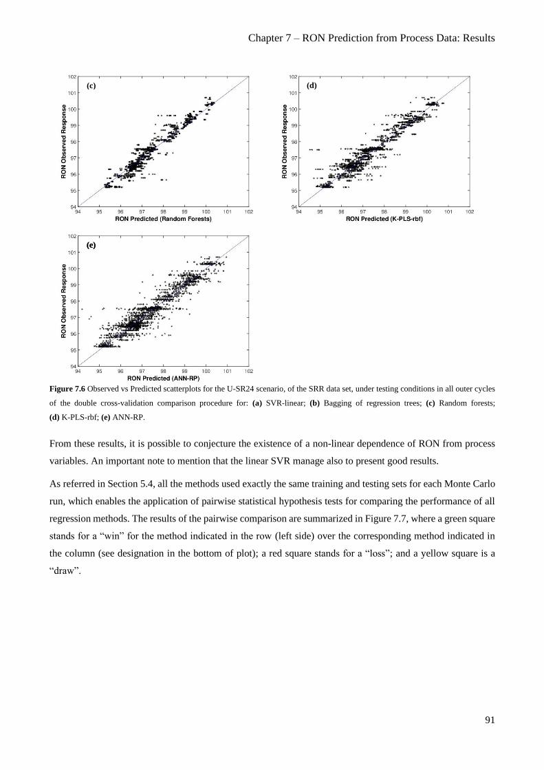
Chapter 7 – RON Prediction from Process Data: Results
91
Figure 7.6 Observed vs Predicted scatterplots for the U-SR24 scenario, of the SRR data set, under testing conditions in all outer cycles
of the double cross-validation comparison procedure for: (a) SVR-linear; (b) Bagging of regression trees; (c) Random forests;
(d) K-PLS-rbf; (e) ANN-RP.
From these results, it is possible to conjecture the existence of a non-linear dependence of RON from process
variables. An important note to mention that the linear SVR manage also to present good results.
As referred in Section 5.4, all the methods used exactly the same training and testing sets for each Monte Carlo
run, which enables the application of pairwise statistical hypothesis tests for comparing the performance of all
regression methods. The results of the pairwise comparison are summarized in Figure 7.7, where a green square
stands for a “win” for the method indicated in the row (left side) over the corresponding method indicated in
the column (see designation in the bottom of plot); a red square stands for a “loss”; and a yellow square is a
“draw”.
(d)
(c) (e)
(c)

Part IV ‒ Results and Discussion
92
Figure 7.7 Heatmap results of the pairwise student’s t -test for the U-SR24 scenario of the SSR data set. A green colour indicates that
the method indicated in the Y-axis is better in a statistically significant sense, over the corresponding method indicated in the X-axis. A
yellow colour indicates that no statistically significant different exists between the methods.
From the pairwise comparison, it is possible to compute the average KPIs that represent the relative performance
of the methods: KPIm and Rankm , where m stands for the method’s index (see Figure 7.8; the results for
( )mKPI s , which are necessary to estimate KPIm and Rankm are presented in Appendix C.1, Table C.1
(page 143).
Figure 7.8 KPIm results for all methods in comparison for the U-SR24 scenario of the SSR data set.
These results confirm the superior predictive accuracy of non-linear methods in the prediction of RON, and in
particular the good performance of the neural network with resilient backpropagation algorithm, bagging of
regression trees and random forests. In particular, ANN-RP has a KPIm value of 18.5 (out of 19), which shows
his superiority over all the remaining methods. This result complements the information given by Figure 7.7,
where ANN-RP “won” over 18 methods and had one “draw” in the pairwise comparison.
As expected, it is possible to verify that the value of KPIm decreases when the methods become less important.

Chapter 7 – RON Prediction from Process Data: Results
93
ii. S-SR st Scenario
Table 7.4, Table 7.5 and Table 7.6 provide the testRMSE ,
2testR and
testPBIAS values, respectively, for all the
regression methods for all the five synchronized single resolution (S-SR st ) scenarios. For this case, the data set
for each scenario has 150 samples and 41 predictors. The difference between each synchronized scenario is the
time support window ( )st used to aggregate the data.
Table 7.4 Average testRMSE under testing conditions considering all Monte Carlo iterations for all the S-SR st scenarios considered
for the SSR data set.
Method S-SR24 S-SR4 S-SR3 S-SR2 S-SR1
MLR 0.891 1.311 1.139 0.883 0.847
FSR 0.924 0.837 0.845 0.798 0.783
RR 0.766 0.797 0.755 0.764 0.779
LASSO 0.800 0.798 0.765 0.774 0.793
EN 0.776 0.804 0.761 0.773 0.791
SVR-poly 0.802 0.830 0.813 0.789 0.828
SVR-rbf 0.794 0.830 0.812 0.788 0.829
SVR-linear 0.749 0.717 0.699 0.726 0.770
PCR 1.069 1.078 1.036 1.042 1.082
PCR-FS 1.119 1.126 1.100 1.103 1.148
PLS 0.812 0.800 0.759 0.774 0.782
Bagging 0.711 0.726 0.673 0.702 0.756
RF 0.716 0.709 0.659 0.710 0.740
Boosting 0.740 0.757 0.698 0.730 0.745
K-PCR-poly 0.966 0.977 0.897 0.939 1.000
K-PCR-rbf 0.764 0.701 0.688 0.692 0.705
K-PLS-poly 1.294 1.254 1.209 1.253 1.236
K-PLS-rbf 0.704 0.685 0.668 0.709 0.725
ANN-LM 0.582 0.567 0.523 0.601 0.608
ANN-RP 0.596 0.573 0.545 0.603 0.581
Table 7.5 Average 2testR under testing conditions considering all Monte Carlo iterations for all the S-SR st scenarios considered for
the SRR data set.
Method S-SR24 S-SR4 S-SR3 S-SR2 S-SR1
MLR 0.590 -0.279 0.173 0.621 0.658
FSR 0.607 0.681 0.662 0.717 0.715
RR 0.726 0.710 0.739 0.740 0.717
LASSO 0.701 0.710 0.733 0.733 0.708
EN 0.721 0.705 0.735 0.734 0.709
SVR-poly 0.699 0.682 0.695 0.722 0.679
SVR-rbf 0.706 0.682 0.696 0.723 0.679
SVR-linear 0.744 0.767 0.776 0.766 0.725

Part IV ‒ Results and Discussion
94
Method S-SR24 S-SR4 S-SR3 S-SR2 S-SR1
PCR 0.482 0.467 0.512 0.516 0.457
PCR-FS 0.429 0.419 0.449 0.457 0.392
PLS 0.695 0.708 0.736 0.732 0.714
Bagging 0.770 0.753 0.788 0.779 0.733
RF 0.767 0.768 0.799 0.774 0.746
Boosting 0.748 0.734 0.775 0.760 0.740
K-PCR-poly 0.577 0.560 0.629 0.604 0.511
K-PCR-rbf 0.732 0.776 0.783 0.787 0.770
K-PLS-poly 0.249 0.289 0.336 0.300 0.307
K-PLS-rbf 0.773 0.787 0.796 0.775 0.755
ANN-LM 0.630 0.660 0.711 0.628 0.596
ANN-RP 0.631 0.653 0.680 0.610 0.639
Table 7.6 Average testPBIAS under testing conditions considering all Monte Carlo iterations for all the S-SR st scenarios considered
for the SRR data set.
Method S-SR24 S-SR4 S-SR3 S-SR2 S-SR1
MLR -0.045 -0.102 -0.031 0.018 0.015
FSR -0.025 -0.005 0.012 -0.059 -0.021
RR -0.055 -0.006 -0.005 0.016 -0.024
LASSO -0.052 -0.022 -0.016 -0.006 -0.038
EN -0.050 -0.015 -0.014 -0.003 -0.030
SVR-poly -0.052 0.001 -0.013 0.001 -0.046
SVR-rbf -0.048 -0.001 -0.011 -0.002 -0.045
SVR-linear -0.008 -0.011 -0.010 0.010 -0.046
PCR -0.021 -0.057 -0.021 -0.003 -0.046
PCR-FS 0.008 -0.015 0.006 -0.069 -0.075
PLS -0.060 -0.001 0.006 0.023 -0.009
Bagging 0.030 -0.022 0.008 -0.032 -0.046
RF 0.008 -0.030 -0.015 -0.041 -0.055
Boosting 0.001 -0.041 -0.014 -0.036 -0.047
K-PCR-poly 0.012 0.050 0.055 -0.002 0.013
K-PCR-rbf -0.038 -0.012 0.001 0.027 -0.007
K-PLS-poly -0.081 -0.021 -0.027 -0.083 -0.058
K-PLS-rbf -0.024 0.049 0.033 0.031 0.027
ANN-LM -0.047 0.042 0.016 0.127 0.034
ANN-RP -0.019 0.058 0.003 0.058 0.051
Regarding the results presented in Table 7.4 and Table 7.5, it is possible to observe that some methods present
an adequate performance in terms of prediction accuracy ( )test 2testRMSE and R , which is a good outcome,
considering that they were obtained with fewer observations (when compared to the case U-SR24). These results
point to a certain advantage of using artificial neural networks methods over the remaining linear and non-linear

Chapter 7 – RON Prediction from Process Data: Results
95
modelling approaches. An overview of the distribution of the testRMSE is provided in Appendix C.1,
Figure C.2, (page 145).
The testPBIAS values, presented in Table 7.6, of the models still allow us to conclude are the models were not
over- or underestimated.
Once again, since all of the methods use exactly the same training and testing set for each Monte Carlo run, it
is possible to conduct a pairwise statistical hypothesis tests to compare the performance of all regression
methods. The pairwise outcomes are summarized in Appendix C.1, Figure C.3 (page 146). The results of the
pairwise comparison were used to estimate the average KPIs ( KPIm ) and are presented in Figure 7.9 for all the
synchronized scenarios. The results for the ( )mKPI s , necessary to compute KPIm and Rankm are presented
in Appendix C.1, Table C.2 to Table C.6 (page 146).
(a) (b)
(c) (d)

Part IV ‒ Results and Discussion
96
Figure 7.9 KPIm results for all methods in comparison for (a) S-SR24; (b) S-SR4; (c) S-SR3; (d) S-SR2; (e) S-SR1.
These results validate the superior predictive accuracy performance achieved with the artificial neural networks.
It is also important to mention the consistency in performance of the neural networks over all the scenarios,
presenting always a KPIm of 18.5 (out of 19).
iii. S-SR1L2 Scenario
Table 7.7 provides the results for the performance indexes of all the regression methods used for the scenario
S-SR1L2. For this case, the data set is composed by 150 samples and 123 predictors.
Table 7.7 Average performance indexes for the S-SR1L2 scenario of the SRR data set, in test conditions, considering all Monte Carlo
iterations for each regression method used.
Resolution Scenario Method testRMSE
2testR test
PBIAS
S-SR1L2
MLR 27.811 -896.827 2.216
FSR 0.800 0.710 -0.009
RR 0.775 0.724 0.033
LASSO 0.759 0.734 0.016
EN 0.760 0.733 0.019
SVR-poly 0.826 0.681 0.044
SVR-rbf 0.826 0.682 0.043
SVR-linear 0.794 0.714 -0.024
PCR 1.053 0.491 0.023
PCR-FS 1.085 0.465 0.010
PLS 0.773 0.722 0.024
Bagging 0.736 0.756 -0.007
RF 0.718 0.768 -0.011
Boosting 0.798 0.708 0.004
K-PCR-poly 1.045 0.489 0.088
K-PCR-rbf 0.786 0.718 -0.005
K-PLS-poly 1.271 0.279 0.010
(e)

Chapter 7 – RON Prediction from Process Data: Results
97
Resolution Scenario Method testRMSE
2testR test
PBIAS
K-PLS-rbf 0.671 0.794 0.034
ANN-LM 0.566 0.654 0.042
ANN-RP 0.661 0.536 0.073
Analysing Table 7.7 it is apparent that the results obtained, with the exception of MLR, present again fairly
reasonable performances in terms of prediction accuracy, in the same range as those achieved in the S-SR st
scenarios. An overview of the distribution of the testRMSE is provided in Appendix C.1, Figure C.4 (page 150),
without the MLR regression since it provided poor results.
For this case, once again, artificial neural networks and kernel partial least squares with radial basis function
present better results over the remaining modelling approaches.
The testPBIAS values, are once again close to zero, which give us the confidence that the models were not
over- or underestimated.
Figure 7.10 presents the Observed versus Predicted scatterplots for the methods with the best predictive
accuracy results, where it is possible to observe that the testing points are relatively close to the 1:1 reference
line.
(a) (b)
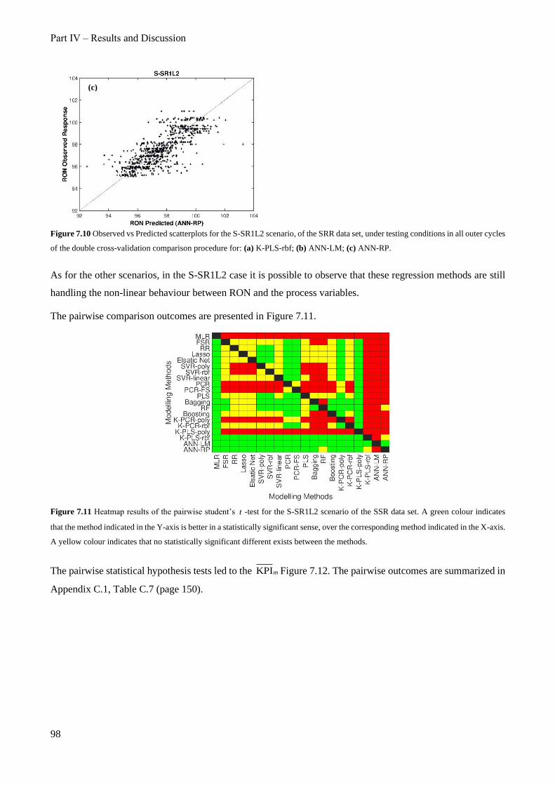
Part IV ‒ Results and Discussion
98
Figure 7.10 Observed vs Predicted scatterplots for the S-SR1L2 scenario, of the SRR data set, under testing conditions in all outer cycles
of the double cross-validation comparison procedure for: (a) K-PLS-rbf; (b) ANN-LM; (c) ANN-RP.
As for the other scenarios, in the S-SR1L2 case it is possible to observe that these regression methods are still
handling the non-linear behaviour between RON and the process variables.
The pairwise comparison outcomes are presented in Figure 7.11.
Figure 7.11 Heatmap results of the pairwise student’s t -test for the S-SR1L2 scenario of the SSR data set. A green colour indicates
that the method indicated in the Y-axis is better in a statistically significant sense, over the corresponding method indicated in the X-axis.
A yellow colour indicates that no statistically significant different exists between the methods.
The pairwise statistical hypothesis tests led to the KPIm Figure 7.12. The pairwise outcomes are summarized in
Appendix C.1, Table C.7 (page 150).
(c)

Chapter 7 – RON Prediction from Process Data: Results
99
Figure 7.12 KPIm results for all methods in comparison for the S-SR1L2 scenario of the SSR data set.
These results confirm, once again, the superiority of the non-linear methods in the prediction of RON. In this
case, the performance of neural network with Levenberg-Marquardt optimization scored the maximum value
(19). From all the scenarios, only in this scenario the maximum value of KPIm was achieved.
7.2. Results for the CCR unit
The CCR data set is composed by 1,048,320 samples for 41 process variables, covering a period of 24 months.
Table 7.8 provides the number of samples collected of RON for the CCR data set, as well as the corresponding
range of values.
Table 7.8 Number of RON samples and the corresponding range, mean and standard deviation.
Property Number of samples Property values
Min. Max. Mean SD
RON 243 96.80 102.50 100.38 0.97
7.2.1. Data Acquisition and Inspection
As happened for the SSR data set, in the case of CCR there is also a well-defined multirate structure, with two
different types of variables: process variables were collected every minute while RON was collected, at best,
once per day. Each recorded value regards an “instantaneous” observation and it is possible to have access to
the time when it was collected. Figure 7.13 gives an overview of the time series of RON and process variable
1X (process variables are anonymized for protecting critical industrial information).

Part IV ‒ Results and Discussion
100
Figure 7.13 (a) Time series plot of RON during the data collection period; (b) Time series plot of 1X during the data collection period.
Analysing Figure 7.13a, there are no observations below the limit value of the product quality and the range
values is smaller when compared with the SRR data set. From Figure 7.13b, is it possible to verify that, in
contrast to the SRR case, there are no non-operation periods due to shutdown or maintenance periods. This
conclusion was validated by the process engineers. As seen in Figure 7.13b, it is possible to verify the existence
of outliers present in the data. The following section provides the results for the data cleaning step, which is the
second step of the data analysis workflow.
Figure 7.14 provides an overview on the level of missing data present in the data set after the data collection
step.
Figure 7.14 Comparison of the percentage of missing data present in the CCR data set.
For variable 1X , there are 222 missing entries out of the 1,048,320 samples (0.02%). From Figure 7.14, it is
possible to verify that the level of missing data is lower when compared with the SRR data set. This happens
because in the CCR data set, there are no non-operations periods.
(a) (b)

Chapter 7 – RON Prediction from Process Data: Results
101
7.2.2. Data Cleaning
The data cleaning of the CCR data followed the same steps as described for the case of the SRR data.
Once again, for illustration purposes, Figure 7.15 presents the results obtained in the cleaning stage of the data
analysis workflow for a process variable, 1X .
Figure 7.15a illustrates the time series for the process variable 1X . The abnormal values present in the data can
be identified by applying an operation filter for each process variable. These abnormal values are Global
outliers. Each process variable has its own operating ranges and Figure 7.15b presents the data for variable 1X
after this stage is conducted (blue line). From the blue line of Figure 7.15b it is possible to observe that there
are still data points left to be removed. These points, were classified as Contextual outliers.
To remove the contextual outliers, three strategies were studied, such as the3 rule, the Hampel identifier and
the modified Hampel identifier with moving window technique.
From Figure 7.15c it is possible to verify that the upper and lower thresholds obtained from the 3 rule do not
identify any of the data points considered as contextual outliers. The Hampel identifier in Figure 7.15d leads to
similar conclusions. Once again, both of these procedures were unable to detect a large fraction of the existing
outliers, since their thresholds are influenced by the existence of outliers, leading to inflated “normal” intervals.
(a) (b)

Part IV ‒ Results and Discussion
102
Figure 7.15 Comparison of various cleaning steps over the same variable 1X : (a) No cleaning filter; (b) Operation filter; (c) 3 filter;
(d) Hampel Identifier; (e) adaptive Hampel identifier with moving window technique. The black line for (c), (e) and (e) represent the
same, they represent the blue line from (b).
The moving window technique is a better alternative, since it does not take into consideration the data set as a
whole, but only considers the local variability for defining the thresholds. Once again, a window size was chosen
for each variable, from a list of possible sizes 50; 500; 1,000; 2,000; 3,000 and 5,000 . The selection of the
most adequate window size was conducted through visual inspection alongside the plant engineers, to reassure
that the points removed were in fact outliers.
From Figure 7.15e it is possible to observe that identification and removal of most of the outliers were
successful. Therefore, like the in the SRR case, the adaptive Hampel algorithm was applied to all the remaining
process variables.
7.2.3. Data Pre-processing
This section provides information about the number of samples, number of predictors and level of missing data
of the different scenarios for the two steps mentioned and for each resolution scenario studied (Table 7.9).
(c) (d)
(e)

Chapter 7 – RON Prediction from Process Data: Results
103
Table 7.9 Number of samples and respective percentage of missing data for each resolution studied.
Resolution Scenario Number of samples Number of predictors Missing data 1X (%)
Collected Data 1,048,320 41 0.02
Data Cleaning 1,048,320 41 3.56
U-SR24 728 41 0.41
S-SR24 243 41 0.00
S-SR4 243 41 0.00
S-SR3 243 41 0.00
S-SR2 243 41 0.00
S-SR1 243 41 0.00
S-SR1L2 243 123 -
Since in this data set there were no non-operation periods to remove, after the data cleaning stage the number
of samples remains the same as the collected data. However, the number of missing data increased, since global
and contextual outliers were replaced by blanks and not removed from the data set.
For the unsynchronized scenario (U-SR24), the data set has 728 new observations, corresponding to the medians
of the aggregation periods. Each observation for the U-SR24 data set represents one day of operation. Variable
1X still has three missing records out of 728, and such an issue needs to be handled through missing data
imputation.
For the synchronized scenarios, the data set has 243 new observations, because in these scenarios, the
aggregation only takes place if there is a record of RON. Since there are 243 samples of RON, the data set after
the synchronized resolution will have the same number of observations. Variable 1X does not have missing
records, but other variables may have, and this issue needs to be taken into consideration.
As mentioned, both methodologies do not eliminate the level of missing data. Figure 7.16, provides an
illustration on how the level of missing data changes for the different single resolution scenarios studied.
Figure 7.16 Comparison of the percentage of missing data, for all variables, before and after the selection of the resolution.

Part IV ‒ Results and Discussion
104
For the CCR data set, as happened in the SRR data set, a robust interpolative method was adopted to estimate
missing records for each scenario. The imputation was carried out via a moving window median approach.
7.2.4. Predictive Assessment
In this section the results related with the Monte Carlo Double Cross-Validation methodologies are presented,
including the performance of the regression methods studied for all the resolution scenarios for the CCR process.
i. U-SR24 Scenario
Table 7.10 provides the average values of the performance metrics obtained of all the regression methods for
the scenario U-SR24. For this case, the data set has 728 samples and 41 predictors.
Table 7.10 Average performance indexes for the U-SR24 scenario, in test conditions, considering all Monte Carlo iterations for each
regression method used.
Resolution Scenario Method testRMSE
2testR test
PBIAS
U-SR24
MLR 0.477 0.689 -0.013
FSR 0.472 0.670 -0.014
RR 0.473 0.670 -0.013
LASSO 0.467 0.703 -0.011
EN 0.468 0.702 -0.012
SVR-poly 0.480 0.685 0.008
SVR-rbf 0.480 0.685 0.008
SVR-linear 0.317 0.863 -0.016
PCR 0.543 0.602 -0.006
PCR-FS 0.602 0.513 -0.014
PLS 0.474 0.670 -0.011
Bagging 0.337 0.846 4.7E-05
RF 0.327 0.856 0.005
Boosting 0.381 0.805 -8.1E-4
K-PCR-poly 0.628 0.471 -0.017
K-PCR-rbf 0.473 0.698 -0.006
K-PLS-poly 0.788 0.170 -0.025
K-PLS-rbf 0.320 0.860 -0.009
ANN-LM 0.640 0.664 0.001
ANN-RP 0.396 0.827 -0.011
From Table 7.10, it is possible to analyse that most of the regression methods present very promising results in
terms of prediction accuracy. In particular there are several methods with an testRMSE value below 0.4. An
overview of the distribution of the testRMSE is given in Appendix C.2, Figure C.5 (page 152).

Chapter 7 – RON Prediction from Process Data: Results
105
These results also point to a certain advantage of using linear SVR, tree-based ensemble, kernel partial least
squares with radial basis function and neural networks (with resilient backpropagation function) over the
remaining modelling approaches.
The Observed versus Predicted scatterplots for the methods are presented in Figure 7.17.
Figure 7.17 Observed vs Predicted scatterplots for the U-SR24 scenario, of the CCR data set under testing conditions in all outer cycles
of the double cross-validation comparison procedure for: (a) SVR-linear; (b) Bagging of regression trees; (c) Random Forests;
(d) K-PLS-rbf; (e) ANN-RP.
Analysing these results, it is possible to observe that the testing points of all the Monte Carlo runs are relatively
(b)
(d) (c)
(e)
(a)

Part IV ‒ Results and Discussion
106
close the 1:1 reference line, which corresponds to a perfect agreement between observed and predicted values.
For the scenarios of the CCR data set it was also applied a pairwise statistical hypothesis tests to compare the
performance of all regression methods. The results of the pairwise comparison are summarized in Figure 7.18.
Figure 7.18 Heatmap results of the pairwise student’s t -test for the U-SR24 scenario of the CCR data set. A green colour indicates that
the method indicated in the Y-axis is better in a statistically significant sense, over the corresponding method indicated in the X-axis. A
yellow colour indicates that no statistically significant different exists between the methods.
From the pairwise comparison, it is possible to compute the average KPIs that summarizes the relative
performance of the methods: KPIm and Rankm , where m stands for the method’s index (see Figure 7.19; (the
results for ( )mKPI s , necessary to calculate KPIm and Rankm , are presented in Appendix C.2, Table C.8,
page 152)).
Figure 7.19 KPIm results for all methods in comparison U-SR24 scenario of the CCR data set.
These results confirm the superior predictive accuracy of non-linear methods in the prediction of RON, and in
particular the good performance of the bagging of regression trees and random forests. Of notice is also the fact
that all ensemble tree-based methods fall in the best five methods.

Chapter 7 – RON Prediction from Process Data: Results
107
ii. S-SR st Scenario
Table 7.11, Table 7.12 and Table 7.13 provides the testRMSE ,
2testR and
testPBIAS values, respectively, for all
the regression methods and for all the five S-SR st scenarios. In this case, the data set for each scenario has 243
samples and 41 predictors.
Table 7.11 Average testRMSE under testing conditions considering all Monte Carlo iterations for all the S-SR st scenarios considered
for the CCR data set.
Method S-SR24 S-SR4 S-SR3 S-SR2 S-SR1
MLR 0.607 0.529 0.637 0.666 0.624
FSR 0.500 0.538 0.548 0.571 0.571
RR 0.494 0.513 0.560 0.578 0.464
LASSO 0.493 0.508 0.502 0.511 0.493
EN 0.486 0.510 0.490 0.500 0.477
SVR-poly 0.533 0.510 0.531 0.558 0.506
SVR-rbf 0.531 0.510 0.530 0.552 0.502
SVR-linear 0.586 0.600 0.561 0.551 0.585
PCR 0.537 0.548 0.530 0.544 0.533
PCR-FS 0.597 0.612 0.606 0.627 0.633
PLS 0.494 0.530 0.502 0.508 0.471
Bagging 0.545 0.595 0.550 0.574 0.599
RF 0.546 0.595 0.561 0.566 0.581
Boosting 0.520 0.559 0.535 0.539 0.539
K-PCR-poly 0.752 0.766 0.731 0.752 0.745
K-PCR-rbf 0.509 0.540 0.517 0.507 0.489
K-PLS-poly 0.918 0.896 0.856 0.880 0.851
K-PLS-rbf 0.510 0.547 0.532 0.544 0.504
ANN-LM 0.852 0.860 0.782 0.725 0.811
ANN-RP 0.690 0.732 0.690 0.692 0.718
Table 7.12 Average 2testR under testing conditions considering all Monte Carlo iterations for all the S-SR st scenarios considered for
the CCR data set.
Method S-SR24 S-SR4 S-SR3 S-SR2 S-SR1
MLR 0.555 0.705 0.505 0.366 0.410
FSR 0.722 0.697 0.660 0.607 0.577
RR 0.730 0.727 0.622 0.549 0.745
LASSO 0.730 0.732 0.719 0.708 0.713
EN 0.738 0.729 0.732 0.717 0.728
SVR-poly 0.681 0.728 0.680 0.630 0.683
SVR-rbf 0.683 0.729 0.681 0.641 0.689
SVR-linear 0.622 0.627 0.649 0.661 0.606
PCR 0.680 0.687 0.686 0.670 0.666

Part IV ‒ Results and Discussion
108
Method S-SR24 S-SR4 S-SR3 S-SR2 S-SR1
PCR-FS 0.605 0.612 0.586 0.553 0.531
PLS 0.729 0.709 0.717 0.709 0.738
Bagging 0.672 0.636 0.663 0.635 0.583
RF 0.674 0.637 0.652 0.644 0.610
Boosting 0.701 0.676 0.681 0.674 0.661
K-PCR-poly 0.376 0.392 0.403 0.353 0.351
K-PCR-rbf 0.714 0.696 0.702 0.711 0.718
K-PLS-poly 0.073 0.166 0.185 0.138 0.163
K-PLS-rbf 0.713 0.687 0.681 0.662 0.695
ANN-LM 0.238 0.287 0.353 0.436 0.269
ANN-RP 0.488 0.485 0.486 0.474 0.413
Table 7.13 Average testPBIAS under testing conditions considering all Monte Carlo iterations for all the S-SR st scenarios considered
for the CCR data set.
Method S-SR24 S-SR4 S-SR3 S-SR2 S-SR1
MLR 0.005 -0.004 -0.052 -0.033 -0.061
FSR 0.026 0.015 -0.034 0.001 -0.030
RR 0.021 0.011 -0.032 -0.007 -0.026
LASSO 0.023 0.011 -0.022 0.008 -0.030
EN 0.024 0.009 -0.021 0.009 -0.029
SVR-poly 0.027 0.008 -0.029 0.017 -0.041
SVR-rbf 0.026 0.009 -0.030 0.018 -0.040
SVR-linear 0.002 0.001 -0.022 0.015 -0.017
PCR 0.015 0.018 -0.014 0.021 -0.021
PCR-FS -0.002 0.012 -0.022 0.002 -0.015
PLS 0.025 0.016 -0.013 0.017 -0.021
Bagging 0.005 0.014 -0.017 0.035 -0.007
RF 0.012 0.021 -0.010 0.027 -0.005
Boosting -0.003 0.016 -0.017 0.013 -0.012
K-PCR-poly -0.012 0.017 -0.027 0.013 -0.016
K-PCR-rbf 0.027 0.026 -0.020 0.018 -0.018
K-PLS-poly 0.017 0.020 -0.024 0.013 -0.004
K-PLS-rbf 0.028 0.013 -0.030 0.008 -0.036
ANN-LM 0.022 0.009 0.027 0.005 -0.021
ANN-RP 0.021 0.021 -0.028 0.001 -0.010
Analysing the results obtained from Table 7.11 and Table 7.12, it is possible to verify that some methods present
an adequate performance regarding prediction accuracy. Most of the regression methods present a testRMSE
value near 0.5, which is very satisfying. These results also point to a certain advantage of using penalized
regression methods, partial least squares and kernel partial least squares with radial basis function over the
remaining linear and non-linear modelling approaches.
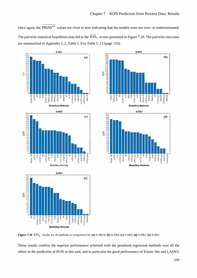
Chapter 7 – RON Prediction from Process Data: Results
109
Once again, the testPBIAS values are close to zero indicating that the models were not over- or underestimated.
The pairwise statistical hypothesis tests led to the KPIm scores presented in Figure 7.20. The pairwise outcomes
are summarized in Appendix C.2, Table C.9 to Table C.13 (page 155).
Figure 7.20 KPIm results for all methods in comparison for (a) S-SR24; (b) S-SR4; (c) S-SR3; (d) S-SR2; (e) S-SR1.
These results confirm the superior performance achieved with the penalized regression methods over all the
others in the prediction of RON in this unit, and in particular the good performance of Elastic Net and LASSO.
(a) (b)
(c) (d)
(e)

Part IV ‒ Results and Discussion
110
In contrast with the SSR case, for the CCR case there are some resolution levels that show superiority over
others. In particular, the S-SR3 scenario, is the only one where the maximum KPIm is achieved.
It is important to mention that the CCR plant has a residence time between two and three hours. That information
can justify the fact that the KPIm has its maximum value (19) precisely for the scenario with a time support of
three hours.
iii. S-SR1L2 Scenario
Table 7.14 provides the performance indexes of all the regression methods for the S-SR1L2 scenario. For this
case, the data set has 223 samples and 132 predictors.
Table 7.14 Average performance indexes for the S-SR1L2 scenario, in test conditions, considering all Monte Carlo iterations for each
regression method used.
Resolution Scenario Method testRMSE
2testR test
PBIAS
S-SR1L2
MLR 0.837 0.122 -0.017
FSR 0.609 0.546 -0.012
RR 0.500 0.702 -0.001
LASSO 0.522 0.670 -0.012
EN 0.531 0.660 -0.010
SVR-poly 0.577 0.593 0.002
SVR-rbf 0.576 0.596 0.003
SVR-linear 0.594 0.583 -0.011
PCR 0.548 0.642 -0.008
PCR-FS 0.606 0.563 -0.018
PLS 0.535 0.655 0.000
Bagging 0.580 0.603 0.005
RF 0.564 0.626 0.006
Boosting 0.532 0.663 0.005
K-PCR-poly 0.782 0.278 0.010
K-PCR-rbf 0.532 0.663 -0.008
K-PLS-poly 0.867 0.119 0.017
K-PLS-rbf 0.520 0.678 0.005
ANN-LM 0.717 0.413 0.002
ANN-RP 0.740 0.382 0.049
Analysing Table 7.14, one can verify that the results obtained present fairly reasonable performances in terms
of prediction accuracy and in the same range as those achieved in the S-SR st . An overview of the distribution
of the testRMSE is provided in Appendix C.2, Figure C.8 (page 159).
Concerning the testPBIAS results, the values are close to zero, which shows that the models were not over- or

Chapter 7 – RON Prediction from Process Data: Results
111
underestimated.
Figure 7.21 presents the Observed versus Predicted scatterplots for the methods with the best predictive
accuracy results.
Figure 7.21 Observed vs Predicted scatterplots for the S-SR1L2 scenario, of the CCR data set, under testing conditions in all outer
cycles of the double cross-validation comparison procedure for (a) ridge regression; (b) LASSO; (c) boosting of regression trees;
(d) K-PLS-rbf.
It is possible to observe that the testing points of all the Monte Carlo runs are relatively close the 1:1 line. This
line corresponds to a perfect agreement between observed and predicted values.
Like in the previous scenarios, once again it was conducted a pairwise statistical hypothesis tests to compare
the performance of all regression methods. The pairwise results are given in Figure 7.22.
(a) (b) (c) (d)

Part IV ‒ Results and Discussion
112
Figure 7.22 Heatmap results of the pairwise student’s t -test for the S-SR1L2 scenario of the CCR data set. A green colour indicates
that the method indicated in the Y-axis is better in a statistically significant sense, over the corresponding method indicated in the X-axis.
A yellow colour indicates that no statistically significant different exists between the methods.
From the results of the pairwise comparison, it was possible to estimate the KPIm scores, which are presented
in Figure 7.23. The pairwise outcomes are summarized in Appendix C.2, Table C.14 (page 159).
Figure 7.23 KPIm results for all methods in comparison for the S-SR1L2 scenario of the CCR data set.
These results confirm the superior predictive accuracy of penalized regression methods in the prediction of
RON, and in particular the good performance of the Ridge Regression. Of notice is also the fact that RR scored
the maximum value (19), meaning that it is statistically more significant than all the other methods.
7.3. Resolution Selection
Since several resolution scenarios were considered, it is of interest to find out which led to the best overall
results.

Chapter 7 – RON Prediction from Process Data: Results
113
7.3.1. SRR Data Set
Considering the SRR data set, in order to select the best resolution scenario only the regression methods with a
KPIm value above 15 were consider. The regression methods that match that criteria are the following: bagging
of regression trees, random forests, kernel partial least squares with radial basis function, neural network with
Levenberg-Marquardt optimization and neural network with resilient back-propagation algorithm. Figure 7.24
provides an overview of the average testRMSE for all the regression methods listed above.
Figure 7.24 Average testRMSE considering all Monte-Carlo iterations for each regression method used for all the scenarios for the
SSR data set.
From Figure 7.24, it is possible to identify that the scenario U-SR24 led to the lowest average testRMSE , for
the case of neural network with resilient backpropagation algorithm. The data set used for U-SR24, is composed
by 523 samples, which are more than in the other scenarios (150). It is important to remember that, in spite of
the high number of samples for U-SR24, some were missing and had to be imputed for use in the training of the
models; however, for testing and computing the testRMSE , only the observed values were considered. The two
neural network regression methods are the best for each synchronized scenario. Considering the synchronized
scenarios, S-SR3 is the one where the neural networks achieved the lowest value of the mean testRMSE . This
result is consistent with the ones obtained in Figure 7.9, since the value for the parameter KPIm is 18.5, near
the maximum value (19).
7.3.2. CCR Data Set
The same methodology described in section 7.3.1, was applied to select the best scenario for the CCR data set.
Figure 7.25 provides an overview of the average testRMSE for all the seven scenarios considered.

Part IV ‒ Results and Discussion
114
Figure 7.25 Average testRMSE considering all Monte-Carlo iterations for each regression method used for all the scenarios for the
CRR data set.
From Figure 7.25, it is possible to identify that the scenario U-SR24 leads to the lowest average testRMSE for
the case of the linear SVR. One important aspect, is the good overall performance of the penalized regression
methods, in particular the ridge regression method. Considering the synchronized scenarios, S-SR3, alongside
with S-SR1, conducted to the best performances, which is consistent with the results obtained in Figure 7.20,
since the value for the parameter KPIm is 18.5, near the maximum value (19).
7.4. Analysis of variables’ importance
The practical interest of deriving predictive methods is not limited to the goal of providing accurate estimates
for the response variable. Another relevant insight is the diagnostic of important variables for explaining the
variability in the response. To further assess the relevance of each variable, a diagnosis of their relative
importance, for each method, was also conducted. Furthermore, a methodology was devised for combining the
variables importance for each method into a global importance measure. The combined metric was derived from
the results of linear predictive methods, as the goal is to analyse the main effects of the variables, which
correspond to the linear part of the relationships, therefore well-captured by these approaches. This methodology
explained in Section 5.4 was conducted for both SRR and CCR data sets and for the U-SR24 scenario.
Table 7.15 presents the 2testR values (from Table 7.3 and Table 7.10) and the respective normalized values (the
normalization of 2testR is presented in Equation (5.6)).
Table 7.15 2testR and 2
testnormR values for all the regression methods tested for the U-SR24 scenario
Data Set Parameter MLR FSR RR LASSO EN PCR PLS
SRR
2testR 0.728 0.711 0.745 0.750 0.750 0.570 0.744
2testnormR 0.878 0.783 0.972 1.000 1.000 0.000 0.967

Chapter 7 – RON Prediction from Process Data: Results
115
Data Set Parameter MLR FSR RR LASSO EN PCR PLS
CCR
2testR 0.689 0.670 0.670 0.703 0.702 0.602 0.513
2testnormR 0.926 0.826 0.826 1.000 0.995 0.468 0.000
After obtaining the normalized coefficients of determination and combining them with the results from the
relative importance (Equation (5.5)), the global importance of each variable was finally computed, using
Equation (5.7). The global importance of each variable thus obtained is shown in Figure 7.26, with an indication
of the industrial section where the process variables came from (more specific information cannot be disclosed
given its industrial strategic relevance for the company).
Figure 7.26 Global importance for all the predictors: (a) SSR data set; (b) CCR data set.
As can be observed from Figure 7.26a, variables 32X , 13X and 37X show up as the three most important ones,
when taking into consideration all the methods under analysis. It is also possible to observe that the most
important variables are the ones related to the reaction zone of the plant. This happens because the RON is
highly dependent on the composition of aromatic and branched paraffinic compounds, which are produced
precisely in the reactor section of the plant.
For the CCR data set, the same conclusions are drowned. From Figure 7.26b, the most important variables are
related to the reaction zone and even with the feed stream, which is also interesting.
The importance of the predictors, for the Random Forests method, was evaluated by their OOB-permuted
predictor delta error, the result of which is illustrated in Figure 7.27.
(a) (b)

Part IV ‒ Results and Discussion
116
Figure 7.27 Importance of the variables for the Random Forest method: (a) SSR data set; (b) CCR data set.
The higher the score, the more important is the predictor for the RON estimate. Figure 7.27a shows that the
variables are important for the RON at different levels. 27X is the most important variable with the score of
0.88, whereas the scores for the other predictor variables range from 0.78 to 0.25. The least important are 1X
and 10X with the score of 0.21. All the predictor variables are involved in the RON model as independent
variables.
Concerning the results from Figure 7.27b, again the variables are important for the RON at different levels. 9X
is the most important variable and 40X the least important. Once again, all the variables are involved in the
RON model as independent variables.
7.5. Analysis of the Catalyst Deactivation Rate
In this section, we address the evolution of the catalyst deactivation and assess the value of its incorporation in
a predictive modelling framework. Most of the deactivation studies referred in the literature are related to the
analysis of the kinetics of the reactions, but here we want to address that problem from a data-driven perspective.
However, this is a complex task, because the phenomenon one is trying to explain, is not directly observable
and measurements cannot be taken about the “current state of catalyst deactivation”. The goals set for this
analysis, are the following: (i) to assess whether it is possible to find surrogate measures of catalyst deactivation
that allow us to overcome the lack of direct measurements; (ii) to preliminary assess the advantage (if any) of
incorporating measures of catalyst deactivation in the predictive modelling frameworks. The following activities
were contemplated to achieve these goals:
1. Develop surrogate measures of catalyst deactivation;
2. Make a preliminary assessment of their validity;
3. Incorporate predictors of catalyst deactivation and build new predictive models for RON;
4. Compare the prediction ability of the new models with explicit catalyst deactivation insights with the
(a) (b)

Chapter 7 – RON Prediction from Process Data: Results
117
former models, developed with explicitly taking into account this phenomenon.
The activities mentioned above, were carried out, and their outcomes are briefly referred below.
The first step is to find a surrogate measure of the catalyst deactivation. This measure needs to reflect the
phenomenon of deactivation and information should be extracted from collected process data. Process insight
points to an important role of reactor temperatures, as they are often used to mitigate the effects of catalyst
deactivation (the use higher temperatures in the reactor to achieve a certain value of RON). Therefore, from the
possible surrogate candidates (feed flow, temperatures, hydrogen pressure and hydrogen flow) the average of
the temperatures at the inlet of the reactor was considered to be the most promising measure.
Figure 7.28 illustrates the variation of both the average inlet temperature of the reactors (WAIT) and RON,
during the period of 523 days in the SRR process. Vertical lines signal the non-operation periods described in
Figure 7.1 (page 84).
Figure 7.28 Time series of the average inlet temperature of the reactors (WAIT) and RON for the SRR process. Time is expressed in
days.
From Figure 7.28 it is clearly visible a trend in the evolution of the reactor temperatures, which confirms that
they may be associated with catalyst deactivation. However, this trend presents some oscillations that are not
justified. Considering that a change in WAIT is likely to have an effect on RON (higher WAIT implying higher
RON), a better solution would be to combine both WAIT and RON in the surrogate metric. The rational is the
following: the effect of catalyst deactivation should be reflected in the RON that is achieved with a certain
WAIT. This ratio changes as a consequence of catalyst deactivation. Therefore, by computing the ratio
RON/WAIT, one may be following more accurately the consequences of catalyst deactivation. The RON/WAIT
ratio for the SRR unit is represented in Figure 7.29.

Part IV ‒ Results and Discussion
118
Figure 7.29 Time series of the RON/WAIT ratio in the SRR unit. Time is expressed in days.
The analysis of Figure 7.29 reveals a clear monotone behaviour of the ratio RON/WAIT, which is likely to
reflect well the unobservable catalyst deactivation phenomenon. The higher values of the ratio in the final period
should be discarded from the analysis, since they are related to the “start and run” cycle of the process unit that
was conducted after the maintenance period.
After validating this RON/WAIT ratio as the surrogate measure, we have proceeded and assessed the impact of
the surrogate measure for improving the performance of the models. To test the hypothesis that taking explicitly
into account the catalyst deactivation phenomenon will improve predictive performance for RON, the surrogate
measure was included as a new predictor together with the remaining process variables from the SSR unit. The
regression methods used were RR and LASSO methods, since they are fast to run and provide a simple way to
evaluate the importance of the variables by analysing their regression coefficients’ values.
Table 7.16 Average performance indexes, in test conditions, considering 10 Monte Carlo iterations for each regression method used.
Regression Method testRMSE 2
testR
Before adding Surrogate RR 0.696 0.745
LASSO 0.688 0.750
After adding Surrogate RR 0.600 0.826
LASSO 0.602 0.824
From Table 7.16, it is possible to verify clear improvements in terms of prediction accuracy, in terms of
testRMSE and 2test R , for the RR and LASSO regression methods.
These preliminary results are very interesting and open new perspectives to further improve the predictive
models presented before. This can be done by investing more efforts in developing better surrogate
measurements, develop models to predict them and finally integrate these models into RON prediction
frameworks.

119
Part V ‒ Conclusions and Future Work
“Data is a precious thing and will last longer than the systems themselves”
Tim Berners-Lee

120
This page was intentionally left in blank

121
Chapter 8. Conclusion
In this work, a detailed data analytics workflow was presented and applied for addressing the challenging but
complex problem of predicting RON in the Catalytic Reforming Units of an oil refinery, using only process
data and identifying the most relevant sources of RON variability. This workflow was implemented as a generic
data analysis platform and includes data cleaning stage and a resolution definition stage, which is goal
dependent. In this thesis, different levels of resolution were tested, together with process dynamic, for
identifying the main variability drivers and obtain models with good prediction accuracy for RON, that could
be used for prediction, monitoring and controlling of the process and to better manage catalyst deactivation – a
phenomenon that spans months of operation in the plant.
A rich variety of predictive methods representative of different classes of regression methodologies was studied
(twenty overall) and compared for the task of RON prediction. This comparison methodology was based on a
Monte Carlo Double Cross-Validation approach, in order to assure for accurate and robust assessments of their
relative predictive merits.
Analysing the results obtained with the different categories of predictive methodologies studied, it is possible
to conclude that for this particular industrial problem, for the SRR data set, the class of neural networks and
ensemble methods based on regression trees provided the best performances. Those methods were able to model
non-linear relationships and the results obtained suggest that a non-linear relationship, together with possible
different relationships across the modelling space, can indeed be present between the predictors and the RON
spaces.
For the CCR data set, the best results were obtained for methods arising from the linear spectrum of predictive
analytics, namely with ridge regression, LASSO and elastic net. From the non-linear methods, kernel partial
least squares with a radial basis function presented also very interesting results considering the several
resolutions studied.
Regarding the different resolution scenarios studied, although the unsynchronized scenario led to the best
results, regarding online implementation in the refinery system, the synchronized scenario should also be
considered. The models that result from the synchronized scenario depend less on imputed values when
compared to the models from the unsynchronized scenario, therefore can be less biased.
Furthermore, these results were also able to diagnose the section of the plant and the specific variables having
more impact over RON variability and estimation capability. This aspect is also critical for the daily operation
of the plant and for sustaining process improvement initiatives aimed at achieving increased performance and
better control, as well as to reduce the influence of disturbances over final product quality. It was thus possible
to conclude that the most important variables for predicting RON are associated with the reaction zone of the
process, something that is in line with the available engineering knowledge about the process, because aromatic

Part V – Conclusions and Future Work
122
and branched paraffins compounds are produced precisely in the reaction area of the plant, and they are believed
to have an important impact over RON values.
The comparison and ranking system proposed in this thesis for the assessment and selection of predictive
methods based on a statistical hypothesis tests were able to quickly identify the best performing approaches,
demonstrating its usefulness in facilitating a quick comprehensive analysis for a large number of methods, and
rational decision support about which ones to explore in industrial practice, given a set of goals to be achieved
and the data available.
Most of the data-driven methods tested with real plant data collected from the refinery led to predictions of
RON values with reasonable accuracy. These values deserve particular consideration, given the existence of
numerous unmeasured sources of variation in a large-scaled industrial process such a refinery, which introduce
non predictive components in the data, as well as possibly some missing elements and noise. From the refinery
operation perspective, as transmitted by its plant engineers, the results obtained are very promising, taking into
account that only process variables are used for coming up with RON estimates, as well as the order of
magnitude for what is considered from a practical industrial point of view as being an acceptable prediction
error (equal or below 0.5).
The results achieved offer good perspectives to future applications in both units of this refinery, as RON is a
critical process outcome and current methods to estimate its values are rather complex, expensive and involve
a long-time delay, until the measurement becomes available. In this work it was shown that using a workflow
composed by statistical and machine learning tools can indeed efficiently lead to quite good results in a short
time, even for rather complex problems, like the prediction of RON values from process variables. These
data-driven models can be instrumental to support process improvement efforts, namely regarding energy
consumption, for instance by avoiding excessive heating in the furnaces and heat exchangers at the inlet of the
reactors, thus also reducing emissions levels and increasing the refinery’s bottom-line results.

123
Chapter 9. Future Work
The work developed during this PhD project can be further extended in future research and can also be replicated
in other unit processes.
Ideally, it would be interesting to consider the hypothesis of implementing onsite the methods obtained, to
further assess the models’ performance with new unseen data, and to optimize the parameters of the respective
models.
Since the synchronized single resolution with lags achieved interesting results, another approach could be the
study of a synchronized multi-resolution scenario. Instead of considering all the variables with the same time
support level (resolution), combining different variables with different time supports, could be an interesting
approach to improve the models.
Regarding the challenge of predicting RON, other type of predictors could be considered. It could be interesting
to combine process variables with laboratorial analysis of the inlet stream of the unit. The composition of the
inlet stream (paraffin, naphthene and aromatic content) and density can contribute with more information in
order to predict RON. Regarding laboratorial analysis, having spectral data of the outlet stream of the unit, can
also have crucial information in order to estimate RON, because RON is highly dependent on the composition
of aromatic and branched paraffinic compounds.
As mentioned above, RON can be linked with the aromatic and branched paraffinic content. These two types
of compounds are produced in the reaction section. Therefore, studying the kinetic of the several reactions that
occur inside the reactors, can be useful to gain insights not only on the RON but on the deactivation rate of the
catalyst. As shown, using as predictor a feature with information regarding the catalyst deactivation, can
improve the prediction of RON. Therefore, it is of interesting to explore this approach in the future.
In this thesis, variable selection was not conducted prior to the implementation of non-linear models (note that
some of them have a built-in variable selection capability, such as Random Forests). Performing a variable
selection or a PCA analysis before the neural network model could be an interesting follow up, since reducing
the number of inputs to feed the neural network could have improvements in prediction errors.
Model maintenance is an important topic that should be researched and improved to avoid the soft sensor
degradation. Since the predictive methods are expected to be implemented on new data sets, it may happen that
the parameters and hyperparameter(s) may require periodic tuning to be more adequate to disturbances in the
new data set.
Another topic that is rising in popularity is Data Fusion. Two main motivations exist for using multiple sensors
and combine them to: (i) reduce errors and uncertainty in the measurements; (ii) use multiple sensors to achieve
a better estimate. In the context of the RON prediction, it could be relevant to use the information available
from three different sources: (i) predictive models; (ii) laboratorial analysis by the motor test; (iii) NIR analysis.

Part V – Conclusions and Future Work
124
This approach is interesting because, in industrial applications, such as this one, it is common to take laboratory
analysis, which provide more accurate measurements of the quality variables, but at slower rates and with
significant delays. To take advantage of this different available sources, is the necessity to properly fuse the data
in question. More information concerning this methodology can be found in (Sansana et al., 2020).

125
References
Ahmad, I., Ali, G., Bilal, M., Chughtai, A., Hussain, A., Kano, M., 2019. Quantitative analysis of product quality
of naphtha reforming process under uncertain process conditions. Chem. Eng. Commun. 1–11.
https://doi.org/10.1080/00986445.2019.1641488
Ahmad, I., Ali, G., Bilal, M., Hussain, A., 2018. Virtual Sensing of Catalytic Naphtha Reforming Process under
Uncertain Feed Conditions, in: International Conference on Computing, Mathematics and Engineering
Technologies. pp. 1–6. https://doi.org/10.1109/ICOMET.2018.8346447
Ahmed, N., Atiya, A., Gayar, N. El, 2010. An Empirical Comparison of Machine Learning Models for Time
Series Forecasting. Econom. Rev. 29, 594–621. https://doi.org/10.1080/07474938.2010.481556
Akaike, H., 1974. A New Look at the Statistical Model Identification. IEEE Trans. Automat. Contr. 19, 716–
723. https://doi.org/10.1109/TAC.1974.1100705
Alpaydin, E., 2004. Introduction to Machine Learning. MIT Press, Cambridge, MA.
Amat-Tosello, S., Dupuy, N., Kister, J., 2009. Contribution of external parameter orthogonalisation for
calibration transfer in short waves - Near infrared spectroscopy application to gasoline quality. Anal.
Chim. Acta 642, 6–11. https://doi.org/10.1016/j.aca.2009.01.003
Amirthalingam, R., Lee, J.H., 1999. Subspace identification based inferential control applied to a continuous
pulp digester. J. Process Control 9, 397–406. https://doi.org/10.1016/S0959-1524(99)00010-4
Andersen, C.M., Bro, R., 2010. Variable selection in regression - a tutorial. J. Chemom. 24, 728–737.
https://doi.org/10.1002/cem.1360
Anderson, J.A., 1997. An Introduction to Neural Networks, 3rd ed. MIT Press, Cambridge.
Anzanello, M.J., Fogliatto, F.S., 2014. A review of recent variable selection methods in industrial and
chemometrics applications. Eur. J. Ind. Eng. 8, 619–645. https://doi.org/0.1504/EJIE.2014.065731
Arteaga, F., Ferrer, A., 2002. Dealing with missing data in MSPC: several methods, different interpretations,
some examples. J. Chemom. 16, 408–418. https://doi.org/10.1002/cem.750
Balabin, R.M., Safieva, R.Z., Lomakina, E.I., 2007. Comparison of linear and nonlinear calibration models
based on near infrared (NIR) spectroscopy data for gasoline properties prediction. Chemom. Intell. Lab.
Syst. 88, 183–188. https://doi.org/10.1016/j.chemolab.2007.04.006
Bao, X., Dai, L., 2009. Partial least squares with outlier detection in spectral analysis: A tool to predict gasoline
properties. Fuel 88, 1216–1222. https://doi.org/10.1016/j.fuel.2008.11.025
Breiman, L., 2001. Random forests. Mach. Learn. 45, 5–32.
https://doi.org/https://doi.org/10.1023/A:1010933404324

126
Breiman, L., Spector, P., 1992. Submodel Selection and Evaluation in Regression. The X-random Case. Int.
Stat. Rev. 60, 291–319. https://doi.org/10.2307/1403680
Burnham, A.J., Macgregor, J.F., Viveros, R., 2001. Interpretation of regression coefficients under a latent
variable regression model. J. Biotechnol. 15, 265–284. https://doi.org/10.1002/cem.680
Burnham, A.J., Macgregor, J.F., Viveros, R., 1999. Latent variable multivariate regression modeling.
Chemometfics Intell. Lab. Syst. 48, 167–180. https://doi.org/10.1016/S0169-7439(99)00018-0
Burnham, A.J., Viveros, R., Macgregor, J.F., 1996. Frameworks for latent variable multirate regression. J.
Chemom. 10, 31–45. https://doi.org/https://doi.org/10.1002/(SICI)1099-128X(199601)10:1<31::AID-
CEM398>3.0.CO;2-1
Cao, D.S., Liang, Y.Z., Xu, Q.S., Hu, Q.N., Zhang, L.X., Fu, G.H., 2011. Exploring nonlinear relationships in
chemical data using kernel-based methods. Chemom. Intell. Lab. Syst. 107, 106–115.
https://doi.org/10.1016/j.chemolab.2011.02.004
Cao, D.S., Xu, Q.S., Liang, Y.Z., Zhang, L.X., Li, H.D., 2010. The boosting: A new idea of building models.
Chemom. Intell. Lab. Syst. 100, 1–11. https://doi.org/10.1016/j.chemolab.2009.09.002
Chauvin, Y., Rumelhart, D.E., 1995. Backpropagation: Theory, Architectures and Applications. Lawrence
Erlbaum Associates, Inc, New Jersey.
Chéruy, A., 1997. Software sensors in bioprocess engineering. J. Biotechnol. 52, 193–199.
https://doi.org/10.1016/S0168-1656(96)01644-6
Chiang, L.H., Pell, R.J., Seasholtz, M.B., 2003. Exploring process data with the use of robust outlier detection
algorithms. J. Process Control 13, 437–449. https://doi.org/10.1016/S0959-1524(02)00068-9
Chiang, L.H., Russel, E.L., Braatz, R.D., 2001. Fault Detection and Diagnosis in Industrial Systems. Springer-
Verlag London. https://doi.org/https://doi.org/10.1007/978-1-4471-0347-9
Chong, I.G., Jun, C.H., 2005. Performance of some variable selection methods when multicollinearity is present.
Chemom. Intell. Lab. Syst. 78, 103–112. https://doi.org/10.1016/j.chemolab.2004.12.011
Curcio, S., Iorio, G., 2013. Models of membrane reactors based on artificial neural networks and hybrid
approaches, in: Handbook of Membrane Reactors. Woodhead Publishing Limited, pp. 569–597.
https://doi.org/10.1533/9780857097330.3.569
David, M., Little, R.J.A., Samuhel, M.E., Triest, R.K., 1986. Alternative Methods for CPS Income Imputation.
J. Am. 81, 29–41. https://doi.org/10.2307/2287965
Davies, L., Gather, U., 1993. The Identification of Multiple Outliers. J. Am. Stat. Assoc. 88, 782.
https://doi.org/10.2307/2290763
de Jong, S., 1993. SIMPLS: an alternative approach to partial least squares regression. Chemom. Intell. Lab.

127
Syst. 18, 251–263. https://doi.org/https://doi.org/10.1016/0169-7439(93)85002-X
Dempster, A.P., Laird, N.M., Rubin, D.B., 1977. Maximum Likelihood from Incomplete Data via the EM
Algorithm. J. R. Stat. Soc. Ser. B 39, 1–38.
Di Bella, A., Fortuna, L., Graziani, S., Napoli, G., Xibilia, M.G., 2007. A Comparative Analysis of the Influence
of Methods for Outliers Detection on the Performance of Data Driven Models, in: Instrumentation and
Measurement Technology Conference. pp. 1–5. https://doi.org/10.1109/IMTC.2007.379222
Dietterich, T.G., 2000. Ensemble Methods in Machine Learning, in: Multiple Classifier Systems. Springer,
Berlin, Heidelberg, pp. 1–15. https://doi.org/10.1007/3-540-45014-9_1
Draper, N.R., Smith, H., 1998. Applied Regression Analysis, 3rd ed, Wiley Series in Probability and Statistics.
John Wiley & Sons, Inc, New York. https://doi.org/10.1002/9781118625590
Elith, J., Leathwick, J.R., Hastie, T., 2008. A working guide to boosted regression trees. J. Anim. Ecol. 77, 802–
813. https://doi.org/10.1111/j.1365-2656.2008.01390.x
Facco, P., Doplicher, F., Bezzo, F., Barolo, M., 2009. Moving average PLS soft sensor for online product quality
estimation in an industrial batch polymerization process. J. Process Control 19, 520–529.
https://doi.org/10.1016/j.jprocont.2008.05.002
Feng, R., Shen, W., Shao, H., 2003. A Soft Sensor Modeling Approach Using Support Vector Machines, in:
Proceedings of the 2003 American Control Conference. IEEE, Denver, Colorado, USA, pp. 3702–3707.
https://doi.org/10.1109/ACC.2003.1240410
Fortuna, L., Graziani, S., Rizzo, A., Xibilia, M.G., 2007. Soft Sensors for Monitoring and Control of Industrial
Processes, 1st ed. Springer-Verlag London, London. https://doi.org/10.1007/978-1-84628-480-9
Fu, Y., Su, H., Zhang, Y., Chu, J., 2008. Adaptive Soft-sensor Modeling Algorithm Based on FCMISVM and
Its Application in PX Adsorption Separation Process. Chinese J. Chem. Eng. 16, 746–751.
https://doi.org/10.1016/S1004-9541(08)60150-0
Galp, 2020. Refining & Marketing [WWW Document]. URL https://www.galp.com/corp/en/about-us/our-
businesses/refining-and-marketing/sourcing-refining-logistics (accessed 2.20.20).
Galp, 2010a. Manual de Operação: Unidade 1300 - Reformação Catalítica Semi-Regenerativa.
Galp, 2010b. Manual de Operação: Unidade 3300 - Reformação Catalítica com Regeneração Contínua de
Catalisador.
Galp, 2008. Memória Descritiva: Fábrica de Combustíveis.
Gary, J.H., Handwerk, G.E., Kaiser, M.J., 2007. Petroleum Refining: Technology and Economics, 5th ed. CRC
Press.
Geisser, S., Eddy, W.F., 1979. A predictive approach to model selection. J. Am. Stat. Assoc. 74, 153–160.

128
https://doi.org/10.1080/01621459.1979.10481632
Geladi, P., 1988. Notes on the history and nature of partial least squares (PLS) modelling. J. Chemom. 2, 231–
246. https://doi.org/10.1002/cem.1180020403
Geladi, P., Esbensen, K., 1991. Regression on multivariate images: Principal component regression for
modeling, prediction and visual diagnostic tools. J. Chemom. 5, 97–111.
https://doi.org/10.1002/cem.1180050206
Geladi, P., Kowalski, B.R., 1986. Partial least-squares regression: a tutorial. Anal. Chim. Acta 185, 1–17.
https://doi.org/10.1016/0003-2670(86)80028-9
Goldberg, D.E., 1989. Genetic Algorithms in Search, Optimization and Machine Learning, 1st ed. Addison-
Wesley Publishing Company, Inc.
Gurney, K., 1997. An Introduction to Neural Networks, 1st ed. UCL Press.
Han, J., Kamber, M., Pei, J., 2012. Data Mining: Concepts and Techniques, 3rd ed, Data Mining: Concepts and
Techniques. Morgan Kaufmann. https://doi.org/10.1016/C2009-0-61819-5
Hastie, T., Tibshirani, R., Friedman, J., 2009. The Elements of Statistical Learning: Data Mining, Inference,
and Prediction, 2nd ed, Springer Series in Statistics. Springer New York, New York, NY.
https://doi.org/10.1007/978-0-387-84858-7
He, K., Cheng, H., Du, W., Qian, F., 2014. Online updating of NIR model and its industrial application via
adaptive wavelength selection and local regression strategy. Chemom. Intell. Lab. Syst. 134, 79–88.
https://doi.org/10.1016/j.chemolab.2014.03.007
Hesterberg, T., Choi, N.H., Meier, L., Fraley, C., 2008. Least angle and L1 penalized regression: A review. Stat.
Surv. 2, 61–93. https://doi.org/10.1214/08-SS035
Hoerl, A.E., Kennard, R.W., 1970. Ridge Regression: Biased Estimation for Nonorthogonal Problems.
Technometrics 12, 55–67. https://doi.org/10.2307/1267351
Hsu, C.S., Robinson, P.R., 2006. Practical Advances in Petroleum Processing. Springer-Verlag New York.
https://doi.org/10.1007/978-0-387-25789-1
Isaksson, A.J., 1992. On the use of linear interpolation in identification subject to missing data; Report EE9202.
Univeristy of Newcastle: Australia.
Jackson, J.E., 1991. A User ’s Guide to Principal Components. John Wiley & Sons.
https://doi.org/10.1002/0471725331
Jackson, J.E., 1980. Principal Components and Factor Analysis: Part 1 - Principal Components. J. Qual.
Technol. 12, 201–213. https://doi.org/10.1080/00224065.1980.11980967
James, G., Witten, D., Hastie, T., Tibshirani, R., 2013. An Introduction to Statistical Learning, Springer Texts

129
in Statistics. Springer Text in Statistics.
Jang, J.O., Chung, H.T., Jeon, G.J., 2005. Saturation and Deadzone Compensation of Systems using Neural
Network and Fuzzy Logic, in: American Control Conference. IEEE, pp. 1715–1720.
https://doi.org/10.1109/acc.2005.1470215
Jianxu, L., Huihe, S., 2003. Soft sensing modeling using neurofuzzy system based on Rough Set Theory, in:
American. pp. 543–548. https://doi.org/10.1109/acc.2002.1024863
Jolliffe, I.T., 2002. Principal Component Analysis, 2nd ed. Springer-Verlag, New York.
https://doi.org/10.1007/b98835
Jones, D.S.J., Pujado, P.R., Treese, S.A., 2006. Handbook of Petroleum Processing.
Kadlec, P., Gabrys, B., Strandt, S., 2009. Data-driven Soft Sensors in the process industry. Comput. Chem. Eng.
33, 795–814. https://doi.org/10.1016/j.compchemeng.2008.12.012
Kadlec, P., Grbić, R., Gabrys, B., 2011. Review of adaptation mechanisms for data-driven soft sensors. Comput.
Chem. Eng. 35, 1–24. https://doi.org/10.1016/j.compchemeng.2010.07.034
Kaneko, H., Arakawa, M., Funatsu, K., 2009. Development of a New Soft Sensor Method Using Independent
Component Analysis and Partial Least Squares. AIChE J. 55, 87–98. https://doi.org/10.1002/aic.11648
Kano, M., Showchaiya, N., Hasebe, S., Hashimoto, I., 2001. Inferential control of distillation compositions:
Selection of model and control configuration. IFAC Proc. Vol. 34, 347–352.
https://doi.org/10.1016/S1474-6670(17)33848-X
Kardamakis, A.A., Pasadakis, N., 2010. Autoregressive modeling of near-IR spectra and MLR to predict RON
values of gasolines. Fuel 89, 158–161. https://doi.org/10.1016/j.fuel.2009.08.029
Khatibisepehr, S., Huang, B., Khare, S., 2013. Design of inferential sensors in the process industry: A review
of Bayesian methods. J. Process Control 23, 1575–1596. https://doi.org/10.1016/j.jprocont.2013.05.007
Kohavi, R., 1995. A Study of Cross-Validation and Bootstrap for Accuracy Estimation and Model Selection,
in: 14th International Joint Conference on Artificial Intelligence. Morgan Kaufmann Publishers Inc., San
Mateo, CA, pp. 1137–1143. https://doi.org/10.1067/mod.2000.109031
Krzanowski, W.J., 1982. Between-Group Comparison of Principal Components - Some Sampling Results. J.
Stat. Comput. Simul. 15, 141–154. https://doi.org/10.1080/00949658208810577
Lababidi, H.M.S., Chedadeh, D., Riazi, M.R., Al-Qattan, A., Al-Adwani, H.A., 2011. Prediction of product
quality for catalytic hydrocracking of vacuum gas oil. Fuel 90, 719–727.
https://doi.org/10.1016/j.fuel.2010.09.046
Leardi, R., 2003. Nature-inspired Methods in Chemometrics: Genetic Algorithms and Artificial Neural
Networks, Data handling in science and technology. Elsevier B.V.

130
Leardi, R., Boggia, R., Terrile, M., 1992. Genetic algorithms as a strategy for feature selection. J. Chemom. 6,
267–281. https://doi.org/10.1002/cem.1180060506
LeCun, Y., Bengio, Y., Hinton, G., 2015. Deep learning. Nature 521, 436–444.
https://doi.org/10.1038/nature14539
Lee, S., Choi, H., Cha, K., Chung, H., 2013. Random forest as a potential multivariate method for near-infrared
(NIR) spectroscopic analysis of complex mixture samples: Gasoline and naphtha. Microchem. J. 110, 739–
748. https://doi.org/10.1016/j.microc.2013.08.007
Lin, B., Recke, B., Jensen, T., Knudsen, J., Jørgensen, S.B., 2006. Product quality estimation using multi-rate
sampled data. Comput. Aided Chem. Eng. 21, 1389–1394. https://doi.org/10.1016/S1570-7946(06)80241-
5
Lin, B., Recke, B., Knudsen, J.K.H., Jorgensen, S.B., 2009. Data-driven soft sensor design with multiple-rate
sampled data: A comparative study. Ind. Eng. Chem. Res. 5379–5387.
https://doi.org/10.23919/ecc.2007.7068500
Lin, B., Recke, B., Knudsen, J.K.H., Jørgensen, S.B., 2007. A systematic approach for soft sensor development.
Comput. Chem. Eng. 31, 419–425. https://doi.org/10.1016/j.compchemeng.2006.05.030
Lindgren, F., Geladi, P., Wold, S., 1993. The Kernel algorithm for PLS. J. Chemom. 7, 45–59.
Little, R.J.A., Rubin, D.B., 2002. Statistical Analysis with Missing Data, 2nd ed. Wiley Series in Probability
and Statistics, Hoboken, New Jersey.
Lu, N., Yang, Y., Gao, F., Wang, F., 2004. Multirate dynamic inferential modeling for multivariable processes.
Chem. Eng. Sci. 59, 855–864. https://doi.org/10.1016/j.ces.2003.12.003
Luo, J.X., Shao, H.H., 2006. Developing soft sensors using hybrid soft computing methodology: a neurofuzzy
system based on rough set theory and genetic algorithms. Soft Comput. 10, 54–60.
https://doi.org/10.1007/s00500-005-0465-0
Macias, J., Angelov, P., Zhou, X., 2006. A Method for Predicting Quality of the Crude Oil Distillation, in: 2006
International Symposium on Evolving Fuzzy Systems. IEEE, Ambleside, pp. 214–220.
https://doi.org/10.1109/ISEFS.2006.251167
Mallows, C.L., 1973. Some comments on Cp. Technometrics 15, 661–675.
https://doi.org/10.1080/00401706.1973.10489103
Marini, F., Bucci, R., Magrì, A.L., Magrì, A.D., 2008. Artificial neural networks in chemometrics: History,
examples and perspectives. Microchem. J. 88, 178–185. https://doi.org/10.1016/j.microc.2007.11.008
Martens, H., Naes, T., 1989. Multivariate Calibration. Wiley, Chichester UK.
McAvoy, T.J., Wang, N.S., Naidu, S., Bhat, N., Hunter, J., Simmons, M., 1989. Interpreting Biosensor Data via

131
Backpropagation, in: International 1989 Joint Conference on Neural Networks. Washington, DC, pp. 227–
233.
Mendes, G., Aleme, H.G., Barbeira, P.J.S., 2012. Determination of octane numbers in gasoline by distillation
curves and partial least squares regression. Fuel 97, 131–136. https://doi.org/10.1016/j.fuel.2012.01.058
Meyers, R.A., 2004. Handbook of Petroleum Refining Processes, 3rd ed. McGraw-Hill Education.
Moghadassi, A., Beheshti, A., Parvizian, F., 2016. Prediction of research octane number in catalytic naphtha
reforming unit of Shazand Oil Refinery. Int. J. Ind. Syst. Eng. 23, 435.
https://doi.org/10.1504/ijise.2016.077696
Montgomery, D.C., Peck, E.A., Vining, G.G., 2012. Introduction to Linear Regression Analysis, 5th ed. New
Jersey.
Montgomery, D.C., Runger, G.C., 2003. Applied Statistics and Probability for Engineers, 3rd ed. John Wiley
& Sons, New York.
Murtaugh, P.A., 1998. Methods of variable selection in regression modeling. Commun. Stat. - Simul. Comput.
27, 711–734. https://doi.org/10.1080/03610919808813505
Naes, T., Isakson, T., Fearn, T., Davies, T., 2004. A user-friendly guide to Multivariate Calibration and
Classification. NIR Publications, Chichester UK.
Næs, T., Mevik, B.H., 2001. Understanding the collinearity problem in regression and discriminant analysis. J.
Chemom. 15, 413–426. https://doi.org/10.1002/cem.676
Nelson, P.R.C., Taylor, P.A., Macgregor, J.F., 1996. Missing data methods in PCA and PLS: Score calculations
with incomplete observations. Chemometfics Intell. Lab. Syst. 35, 45–65. https://doi.org/10.1016/S0169-
7439(96)00007-X
Park, S., Han, C., 2000. A nonlinear soft sensor based on multivariate smoothing procedure for quality
estimation in distillation columns. Comput. Chem. Eng. 24, 871–877. https://doi.org/10.1016/S0098-
1354(00)00343-4
Pearson, R.K., 2002. Outliers in process modeling and identification. IEEE Trans. Control Syst. Technol. 10,
55–63. https://doi.org/10.1109/87.974338
Pearson, R.K., 2001. Exploring process data. J. Process Control 11, 179–194. https://doi.org/10.1016/S0959-
1524(00)00046-9
Qin, J.S., 1998. Recursive PLS algorithms for adaptive data modeling. Comput. Chem. Eng. 22, 503–514.
https://doi.org/10.1016/S0098-1354(97)00262-7
Qin, S.J., 1997. Neural Networks for Intelligent Sensors and Control - Practical Issues and Some Solutions, in:
Neural Systems for Control. pp. 215–236. https://doi.org/10.1016/b978-012526430-3/50009-x

132
Ramachandran, P., Young, G.E., Misawa, E.A., 1996. Intersample output estimation with multirate sampling,
in: IEEE Conference on Control Applications - Proceedings. pp. 576–581.
https://doi.org/10.1109/cca.1996.558924
Rantalainen, M., Bylesjo, M., Cloarec, O., Nicholson, J.K., Holmes, E., Trygg, J., 2007. Kernel based
orthogonal projections to latent structures (K-OPLS). J. Chemom. 21, 376–385.
https://doi.org/10.1002/cem.1071
Rasmussen, M.A., Bro, R., 2012. A tutorial on the Lasso approach to sparse modeling. Chemom. Intell. Lab.
Syst. 119, 21–31. https://doi.org/10.1016/j.chemolab.2012.10.003
Rato, T.J., Reis, M.S., 2017. Multiresolution Soft Sensors: A New Class of Model Structures for Handling
Multiresolution Data. Ind. Eng. Chem. Res. 56, 3640–3654. https://doi.org/10.1021/acs.iecr.6b04349
Reis, M.S., 2019. Multiscale and multi-granularity process analytics: A review. Processes 7, 1–21.
https://doi.org/10.3390/pr7020061
Rendall, R., Reis, M.S., 2018. Which regression method to use? Making informed decisions in “data-
rich/knowledge poor” scenarios – The Predictive Analytics Comparison framework (PAC). Chemom.
Intell. Lab. Syst. 181, 52–63. https://doi.org/10.1016/j.chemolab.2018.08.004
Rosipal, R., Trejo, L.J., 2001. Kernel Partial Least Squares Regression in Reproducing Kernel Hilbert Space. J.
Mach. Learn. Res. 2, 97–123. https://doi.org/10.1162/15324430260185556
Rumelhart, D.E., Hinton, G.E., Williams, R.J., 1986. Learning Internal Representations by Error Propagation,
in: Parallel Distributed Processing: Explorations in the Microstructure of Cognition: Foundations. MIT
Press, Cambridge, MA, pp. 319–362.
Sadighi, S., Mohaddecy, R.S., 2013. Predictive Modeling for an Industrial Naphtha Reforming Plant using
Artificial Neural Network with Recurrent Layers. Int. J. Technol. 4, 102–111.
https://doi.org/10.14716/ijtech.v4i2.106
Sansana, J., Rendall, R., Wang, Z., Chiang, L.H., Reis, M.S., 2020. Sensor Fusion with Irregular Sampling and
Varying Measurement Delays. Ind. Eng. Chem. Res. 59, 2328–2340.
https://doi.org/10.1021/acs.iecr.9b05105
Schafer, J.L., 1999. Statistical Methods in Medical Research. Stat. Methods Med. Res. 8, 3–15.
https://doi.org/10.1177/096228029900800102
Schafer, J.L., 1997. Analysis of Incomplete Multivariate Data. Chapman & Hall.
Schafer, J.L., Olsen, M.K., Schafer, J.L., Olsen, M.K., 1998. Multiple Imputation for Multivariate Missing-Data
Problems : A Data Analyst ’ s Perspective Missing-Data Problems: A Data Analyst ’s Perspective.
Multivariate Behav. Res. 33, 545–571. https://doi.org/10.1207/s15327906mbr3304_5
Scheffer, J., 2002. Dealing With Missing Data. Res. Lett. Inf. Math. Sci. 3, 153–160.

133
https://doi.org/10.1016/j.pmrj.2015.07.011
Schenatto, K., de Souza, E.G., Bazzi, C.L., Gavioli, A., Betzek, N.M., Beneduzzi, H.M., 2017. Normalization
of data for delineating management zones. Comput. Electron. Agric. 143, 238–248.
https://doi.org/10.1016/j.compag.2017.10.017
Scholkopf, B., Smola, A., Muller, K.-R., 1998. Nonlinear Component Analysis as a Kernel Eigenvalue Problem.
Neural Comput. 10, 1299–1319. https://doi.org/10.1162/089976698300017467
Scholkopf, B., Smola, A.J., 2002. Learning with Kernels: Support Vector Machines, Regularization,
Optimization, and Beyond. MIT Press.
Schwarz, H., 1978. Estimating the dimension of a model. Ann. Stat. 6, 590–606.
https://doi.org/10.1214/aos/1176344136
Seborg, D.E., Edgar, T.F., Mellichamp, D.A., 2011. Process Dynamics and Control, 3rd ed. John Wiley & Sons.
Shakil, M., Elshafei, M., Habib, M.A., Maleki, F., 2009. Soft Sensor for NOx and O2 Using Dynamical Neural
Network. Comput. Electr. Eng. 35, 578–586. https://doi.org/10.1016/j.compeleceng.2008.08.007
Singh, D., Singh, B., 2019. Investigating the impact of data normalization on classification performance. Appl.
Soft Comput. J. https://doi.org/10.1016/j.asoc.2019.105524
Smola, A.J., Scholkopf, B., 2004. A tutorial on support vector regression. Stat. Comput. 14, 199–222.
https://doi.org/10.1023/B:STCO.0000035301.49549.88
Sofge, D.A., 2002. Using Genetic Algorithm Based Variable Selection to Improve Neural Network Models for
Real-World Systems, in: Proceedings of the 2002 International Conference on Machine Learning and
Applications. pp. 16–19.
Souza, F.A.A., Araújo, R., Mendes, J., 2016. Review of soft sensor methods for regression applications.
Chemom. Intell. Lab. Syst. 152, 69–79. https://doi.org/10.1016/j.chemolab.2015.12.011
Stephanopoulos, G., Han, C., 1996. Intelligent Systems in Process Engineering: A review. Comput. Chem. Eng.
20, 743–791. https://doi.org/10.1016/0098-1354(95)00194-8
Stone, M., 1974. Cross-validatory Choice and Assessment of Statistical Predictions. J. R. Stat. Soc. Ser. B 36,
111–133. https://doi.org/10.1111/j.2517-6161.1974.tb00994.x
Strobl, C., Malley, J., Gerhard T, 2009. An Introduction to Recursive Partitioning: Rationale, Application and
Characteristics of Classification and Regression Trees, Bagging and Random Forests. Psychol. Methods
14, 323–348. https://doi.org/10.1037/a0016973
Tibshirani, R., 1996. Regression Shrinkage and Selection via the Lasso. J. R. Stat. Soc. Ser. B (Statistical
Methodol. 58, 267–288. https://doi.org/10.1111/j.2517-6161.1996.tb02080.x
van der Baan, M., Jutten, C., 2010. Neural networks in geophysical applications. Geophysics 65, 1032–1047.

134
https://doi.org/10.1190/1.1444797
Vapnik, N.V., 2000. The Nature of Statistical Learning Theory, 2nd ed. Springer-Verlag.
https://doi.org/10.1007/978-1-4757-3264-1
Venkatasubramanian, V., Vaidyanathan, R., Yamamoto, Y., 1990. Process fault detection and diagnosis using
neural networks - I. steady-state processes. Comput. Chem. Eng. 14, 699–712.
https://doi.org/10.1016/0098-1354(90)87081-Y
Vert, J.-P., Tsuda, K., Scholkopf, B., 2004. A Primer on Kernel Methods, in: Kernel Methods in Computational
Biology. MIT Press. https://doi.org/10.7551/mitpress/4057.003.0004
Vezvaei, H., Ordibeheshti, S., Ardjmand, M., 2011. Soft-Sensor for Estimation of Gasoline Octane Number in
Platforming Processes with Adaptive Neuro-Fuzzy Inference Systems (ANFIS). Int. J. Chem. Mol. Nucl.
Mater. Metall. Eng. 5, 261–265.
Vitale, R., Palací-López, D., Kerkenaar, H.H.M., Postma, G.J., Buydens, L.M.C., Ferrer, A., 2018. Kernel-
Partial Least Squares regression coupled to pseudo-sample trajectories for the analysis of mixture designs
of experiments. Chemom. Intell. Lab. Syst. 175, 37–46. https://doi.org/10.1016/j.chemolab.2018.02.002
Voigt, M., Legner, R., Haefner, S., Friesen, A., Wirtz, A., Jaeger, M., 2019. Using fieldable spectrometers and
chemometric methods to determine RON of gasoline from petrol stations: A comparison of low-field1H
NMR@80 MHz, handheld RAMAN and benchtop NIR. Fuel 236, 829–835.
https://doi.org/10.1016/j.fuel.2018.09.006
Walczak, B., Massart, D.L., 2001a. Dealing with missing data: Part I. Chemom. Intell. Lab. Syst. 58, 15–27.
https://doi.org/10.1016/S0169-7439(01)00131-9
Walczak, B., Massart, D.L., 2001b. Dealing with missing data: Part II. Chemom. Intell. Lab. Syst. 58, 29–42.
https://doi.org/10.1016/S0169-7439(01)00132-0
Wang, J., Chen, T., Huang, B., 2004. Multirate sampled-data systems: Computing fast-rate models. J. Process
Control 14, 79–88. https://doi.org/10.1016/S0959-1524(03)00033-7
Wang, L.X., Mendel, J.M., 1992. Fuzzy Basis Functions, Universal Approximation, and Orthogonal Least-
Squares Learning. IEEE Trans. Neural Networks 3, 807–814. https://doi.org/10.1109/72.159070
Wang, M., Yan, G., Fei, Z., 2015. Kernel PLS based prediction model construction and simulation on theoretical
cases. Neurocomputing 165, 389–394. https://doi.org/10.1016/j.neucom.2015.03.028
Warne, K., Prasad, G., Rezvani, S., Maguire, L., 2004. Statistical and computational intelligence techniques for
inferential model development: A comparative evaluation and a novel proposition for fusion. Eng. Appl.
Artif. Intell. 17, 871–885. https://doi.org/10.1016/j.engappai.2004.08.020
Willis, M.J., Di Massimo, C., Montague, G.A., Tham, M.T., Morris, A.J., 1991. Artificial neural networks in
process engineering. IEE Proc. D Control Theory Appl. 138, 256–266. https://doi.org/10.1049/ip-
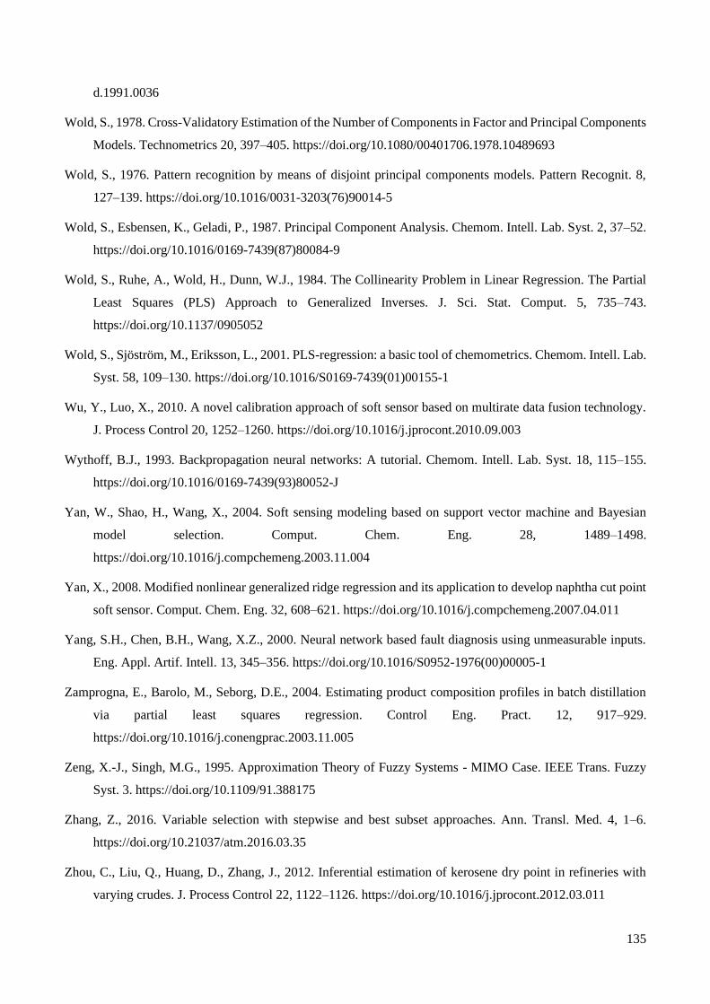
135
d.1991.0036
Wold, S., 1978. Cross-Validatory Estimation of the Number of Components in Factor and Principal Components
Models. Technometrics 20, 397–405. https://doi.org/10.1080/00401706.1978.10489693
Wold, S., 1976. Pattern recognition by means of disjoint principal components models. Pattern Recognit. 8,
127–139. https://doi.org/10.1016/0031-3203(76)90014-5
Wold, S., Esbensen, K., Geladi, P., 1987. Principal Component Analysis. Chemom. Intell. Lab. Syst. 2, 37–52.
https://doi.org/10.1016/0169-7439(87)80084-9
Wold, S., Ruhe, A., Wold, H., Dunn, W.J., 1984. The Collinearity Problem in Linear Regression. The Partial
Least Squares (PLS) Approach to Generalized Inverses. J. Sci. Stat. Comput. 5, 735–743.
https://doi.org/10.1137/0905052
Wold, S., Sjöström, M., Eriksson, L., 2001. PLS-regression: a basic tool of chemometrics. Chemom. Intell. Lab.
Syst. 58, 109–130. https://doi.org/10.1016/S0169-7439(01)00155-1
Wu, Y., Luo, X., 2010. A novel calibration approach of soft sensor based on multirate data fusion technology.
J. Process Control 20, 1252–1260. https://doi.org/10.1016/j.jprocont.2010.09.003
Wythoff, B.J., 1993. Backpropagation neural networks: A tutorial. Chemom. Intell. Lab. Syst. 18, 115–155.
https://doi.org/10.1016/0169-7439(93)80052-J
Yan, W., Shao, H., Wang, X., 2004. Soft sensing modeling based on support vector machine and Bayesian
model selection. Comput. Chem. Eng. 28, 1489–1498.
https://doi.org/10.1016/j.compchemeng.2003.11.004
Yan, X., 2008. Modified nonlinear generalized ridge regression and its application to develop naphtha cut point
soft sensor. Comput. Chem. Eng. 32, 608–621. https://doi.org/10.1016/j.compchemeng.2007.04.011
Yang, S.H., Chen, B.H., Wang, X.Z., 2000. Neural network based fault diagnosis using unmeasurable inputs.
Eng. Appl. Artif. Intell. 13, 345–356. https://doi.org/10.1016/S0952-1976(00)00005-1
Zamprogna, E., Barolo, M., Seborg, D.E., 2004. Estimating product composition profiles in batch distillation
via partial least squares regression. Control Eng. Pract. 12, 917–929.
https://doi.org/10.1016/j.conengprac.2003.11.005
Zeng, X.-J., Singh, M.G., 1995. Approximation Theory of Fuzzy Systems - MIMO Case. IEEE Trans. Fuzzy
Syst. 3. https://doi.org/10.1109/91.388175
Zhang, Z., 2016. Variable selection with stepwise and best subset approaches. Ann. Transl. Med. 4, 1–6.
https://doi.org/10.21037/atm.2016.03.35
Zhou, C., Liu, Q., Huang, D., Zhang, J., 2012. Inferential estimation of kerosene dry point in refineries with
varying crudes. J. Process Control 22, 1122–1126. https://doi.org/10.1016/j.jprocont.2012.03.011

136
Zou, H., Hastie, T., 2005. Regularization and variable selection via the elastic net. J. R. Stat. Soc. Ser. B
(Statistical Methodol. 67, 301–320. https://doi.org/10.1111/j.1467-9868.2005.00503.x

137
Appendices

138
This page was intentionally left in blank

139
Appendix A Pseudo-codes for Resolution Selection
This appendix, provides the pseudo-codes concerning the unsynchronized and synchronized single resolution
approaches.
A.1. Unsynchronized Single Resolution (U-SRS
t )
Table A.1 refers to the pseudo-code for the unsynchronized single resolution with a time support of st . The
scenario U-SR24 follow this strategy.
Table A.1 Pseudo-code for establishing unsynchronized data resolution.
Algorithm Aggregation at a time support st
Input A data set ( )X , selected time support ( )st
1. Obtain the original ( )n number of samples of X and the new number of samples after the aggregation operation ( )newn ;
2. For each variable ( )j , compute the coarser resolution values by applying the median in each aggregation window.
Output A data set at time support st : newX
( )( ) ( )
( )
S
, ,
, size(X)
T
for 1:
for = 1:
1 1 :
nanmedian
end
end
aux
new
new
aux s s
i j idx j
n m
nn floor
j m
i n
idx i t i t
Xnew X
=
=
=
= − +
=

140
A.2. Synchronized Single Resolution (S-SRS
t )
Table A.2 refers to the pseudo-code for the synchronized single resolution scenario at a time support of st . The
scenarios S-SR24, S-SR4, S-SR3, S-SR2 and S-SR1 follow this calculation.
Table A.2 Pseudo-code for establishing synchronized data resolution.
Algorithm Aggregation at a time support st
Input A data set ( )X , output vector ( )y , selected time support ( )st
1. Obtain the indexes of values for ( )y ;
2. For each variable ( )j , compute the coarser resolution values by applying the median in each aggregation window.
Output A data set at time support st : newX
( )( )
( )
( )
( )
( ), : ,
, size(X)
find ~ isnan
for 1:
for = 1:size ,1
nanmedian
end
end
start end
index
index
start index s
end index
k j i i j
n m
y y
j m
k y
i y k t
i y k
Xnew X
=
=
=
= −
=
=

141
A.3. Synchronized Single Resolution with Lags
Table A.3 refers to the pseudo-code for the synchronized single resolution scenario at a time support of st with
lag level. The scenario S-SR1L2 follow this calculation.
Table A.3 Pseudo-code for establishing synchronized data resolution with lag level.
Algorithm Aggregation at a time support st with lag level
Input A data set ( )X , selected time support ( )st , selected lag level ( )lag
1. Obtain the indexes of values for ( )y ;
2. For each variable ( )j , compute the coarser resolution values by applying the median in each aggregation window.
Output A data set at time support st with lag levels: rX
( )( )
( )
, size(X)
find ~ isnan
0 : lag
0
for 1: size ,1
for = 1:
1
for 1: size( ,1)
index
Tvector
counter
lag vector
counter counter
index
end index
n m
y y
lag
lag
i lag
j m
lag lag
k y
i y
=
=
=
=
=
= +
=
= ( )
( ), ,
( )
nanmedian ,
end
end
end
start end
vector lag s
start end s
k j i i
k lag i t
i i t
Xnew X j
−
= −
=

142
Appendix B Hyperparameters of the Regression Methods
In this appendix, is presented the range of the hyperparameter(s) used in the regression methods, as well as their
selection strategy.
Table B.1 Hyperparameter(s) for each method used during the model training stage.
Method Hyperparameter(s) Possible value(s) Selection strategy
MLR - - -
FSR inp
outp
0.05
0.10 -
PCR PCRa 1: min(20, , )n p 10-fold cv
PCR-FS inp
outp
0.05
0.10 10-fold cv
PLS PLSa 1: min(20, , )n p 10-fold cv
RR
0
0.001; 0.01; 0.1; 1; 10 10-fold cv
LASSO
1
0.001; 0.01; 0.1; 1; 10 10-fold cv
EN
0; 0.167; 0.333; 0.500; 0.667; 0.833; 1
0.001; 0.01; 0.1; 1; 10 10-fold cv
BRT BRTT 50; 100; 500; 1000; 5000 10-fold cv
RF RFT 50; 100; 500; 1000; 5000 10-fold cv
BT BTT 50; 100; 500; 1000; 5000 10-fold cv
SVR-linear linear 0.001; 0.005; 0.01; 0.05; 0.1 10-fold cv
SVR-poly rbf 0.001; 0.005; 0.01; 0.05; 0.1 10-fold cv
SVR-rbf poly 0.001; 0.005; 0.01; 0.05; 0.1 10-fold cv
K-PCR-poly PCRa
polyp
1: 30
2; 4; 6; 8; 10 10-fold cv
K-PCR-rbf PCRa
rbfp
1:30
0.1; 1; 10; 50; 100; 300; 1000 10-fold cv
K-PLS-poly PLSa
polyp
1: 30
2; 4; 6; 8; 10 10-fold cv
K-PLS-rbf PCRa
rbfp
1:30
0.1; 1; 10; 50; 100; 300; 1000 10-fold cv
ANN-LM layer
LMn
1
5; 10; 15 10-fold cv
ANN-RP layer
RPn
1
5; 10; 15 10-fold cv

143
Appendix C Predictive Assessment - Complementary Results
This appendix provides the complementary results regarding the regression methods presented in Section 7.1.4
(SRR data set) and Section 7.2.4 (CCR data set).
C.1. Predictive Assessment SRR Data Set
i. U-SR24 Scenario
This section presents all the complementary results for the U-SR24 scenario of the SRR data set.
Figure C.1 presents the distribution of the testRMSE considering all the Monte Carlo iterations for each
regression method studied.
Figure C.1 Box plot of the testRMSE , for the U-SR24 scenario for the SRR data set, considering all the considering all Monte Carlo
iterations for each regression method used.
Table C.1 presents the ( )KPI s values depending on the “draw” score, for the calculation of the Mean KPI and
Mean Rank present in Equations (5.2) and (5.3).
Table C.1 Results of the ( )KPI s for the U-SR24 scenario for the SRR data set.
Method s
KPIm 0.0 0.1 0.2 0.3 0.4 0.5 0.6 0.7 0.8 0.9 1.0
MLR 4.0 4.8 5.6 6.4 7.2 8.0 8.8 9.6 10.4 11.2 12.0 8.0
FSR 3.0 3.7 4.4 5.1 5.8 6.5 7.2 7.9 8.6 9.3 10.0 6.5
RR 6.0 6.6 7.2 7.8 8.4 9.0 9.6 10.2 10.8 11.4 12.0 9.0
LASSO 8.0 8.4 8.8 9.2 9.6 10.0 10.4 10.8 11.2 11.6 12.0 10.0
EN 7.0 7.5 8.0 8.5 9.0 9.5 10.0 10.5 11.0 11.5 12.0 9.5

144
Method s
KPIm 0.0 0.1 0.2 0.3 0.4 0.5 0.6 0.7 0.8 0.9 1.0
SVR-poly 3.0 3.5 4.0 4.5 5.0 5.5 6.0 6.5 7.0 7.5 8.0 5.5
SVR-rbf 3.0 3.5 4.0 4.5 5.0 5.5 6.0 6.5 7.0 7.5 8.0 5.5
SVR-linear 14.0 14.2 14.4 14.6 14.8 15.0 15.2 15.4 15.6 15.8 16.0 15.0
PCR 2.0 2.1 2.2 2.3 2.4 2.5 2.6 2.7 2.8 2.9 3.0 2.5
PCR-FS 1.0 1.1 1.2 1.3 1.4 1.5 1.6 1.7 1.8 1.9 2.0 1.5
PLS 6.0 6.4 6.8 7.2 7.6 8.0 8.4 8.8 9.2 9.6 10.0 8.0
Bagging 16.0 16.2 16.4 16.6 16.8 17.0 17.2 17.4 17.6 17.8 18.0 17.0
RF 16.0 16.2 16.4 16.6 16.8 17.0 17.2 17.4 17.6 17.8 18.0 17.0
Boosting 13.0 13.1 13.2 13.3 13.4 13.5 13.6 13.7 13.8 13.9 14.0 13.5
K-PCR-poly 3.0 3.5 4.0 4.5 5.0 5.5 6.0 6.5 7.0 7.5 8.0 5.5
K-PCR-rbf 12.0 12.1 12.2 12.3 12.4 12.5 12.6 12.7 12.8 12.9 13.0 12.5
K-PLS-poly 0.0 0.1 0.2 0.3 0.4 0.5 0.6 0.7 0.8 0.9 1.0 0.5
K-PLS-rbf 14.0 14.2 14.4 14.6 14.8 15.0 15.2 15.4 15.6 15.8 16.0 15.0
ANN-LM 0.0 1.9 3.8 5.7 7.6 9.5 11.4 13.3 15.2 17.1 19.0 9.5
ANN-RP 18.0 18.1 18.2 18.3 18.4 18.5 18.6 18.7 18.8 18.9 19.0 18.5
ii. S-SRst Scenario
This section presents all the complementary results for the five S-SR st scenarios of the SRR data set.
Figure C.2 presents the distribution of the testRMSE considering all the Monte Carlo iterations for each
regression method studied.
(a)
(b)

145
Figure C.2 Box plot of the testRMSE , for the SRR data set, considering all the considering all Monte Carlo iterations for each regression
method used for all the S-SR st scenarios: (a) S-SR24: (b) S-SR4; (c) S-SR3; (d) S-SR2; (e) S-SR1.
Figure C.3 presents the results of the pairwise student’s t -test for all the synchronized scenarios.
(c) (d)
(e)
(a) (b)

146
Figure C.3 Heatmap results of the pairwise student’s t -test. for the SSR data set, considering all the considering all Monte Carlo
iterations for each regression method used for all the S-SR st scenarios: (a) S-SR24: (b) S-SR4; (c) S-SR3; (d) S-SR2; (e) S-SR1. A
green colour indicates that the method indicated in the Y-axis is better in a statistically significant sense, over the corresponding method
indicated in the X-axis. A yellow colour indicates that no statistically significant different exists between the methods.
Table C.2 presents the ( )KPI s values depending on the “draw” score, for the calculation of the Mean KPI and
Mean Rank present in Equations (5.2) and (5.3) for the S-SR24 scenario.
Table C.2 Results of the ( )KPI s for the S-SR24 scenario for the SRR data set.
Method s
KPIm 0.0 0.1 0.2 0.3 0.4 0.5 0.6 0.7 0.8 0.9 1.0
MLR 3.0 4.0 5.0 6.0 7.0 8.0 9.0 10.0 11.0 12.0 13.0 8.0
FSR 3.0 3.2 3.4 3.6 3.8 4.0 4.2 4.4 4.6 4.8 5.0 4.0
RR 10.0 10.6 11.2 11.8 12.4 13.0 13.6 14.2 14.8 15.4 16.0 13.0
LASSO 5.0 5.7 6.4 7.1 7.8 8.5 9.2 9.9 10.6 11.3 12.0 8.5
EN 8.0 8.8 9.6 10.4 11.2 12.0 12.8 13.6 14.4 15.2 16.0 12.0
SVR-poly 5.0 5.6 6.2 6.8 7.4 8.0 8.6 9.2 9.8 10.4 11.0 8.0
SVR-rbf 6.0 6.7 7.4 8.1 8.8 9.5 10.2 10.9 11.6 12.3 13.0 9.5
SVR-linear 5.0 6.2 7.4 8.6 9.8 11.0 12.2 13.4 14.6 15.8 17.0 11.0
PCR 2.0 2.0 2.0 2.0 2.0 2.0 2.0 2.0 2.0 2.0 2.0 2.0
PCR-FS 1.0 1.0 1.0 1.0 1.0 1.0 1.0 1.0 1.0 1.0 1.0 1.0
PLS 5.0 5.6 6.2 6.8 7.4 8.0 8.6 9.2 9.8 10.4 11.0 8.0
(c) (d)
(e)

147
Method s
KPIm 0.0 0.1 0.2 0.3 0.4 0.5 0.6 0.7 0.8 0.9 1.0
Bagging 10.0 10.7 11.4 12.1 12.8 13.5 14.2 14.9 15.6 16.3 17.0 13.5
RF 10.0 10.7 11.4 12.1 12.8 13.5 14.2 14.9 15.6 16.3 17.0 13.5
Boosting 5.0 6.2 7.4 8.6 9.8 11.0 12.2 13.4 14.6 15.8 17.0 11.0
K-PCR-poly 3.0 3.2 3.4 3.6 3.8 4.0 4.2 4.4 4.6 4.8 5.0 4.0
K-PCR-rbf 6.0 7.0 8.0 9.0 10.0 11.0 12.0 13.0 14.0 15.0 16.0 11.0
K-PLS-poly 0.0 0.0 0.0 0.0 0.0 0.0 0.0 0.0 0.0 0.0 0.0 0.0
K-PLS-rbf 13.0 13.4 13.8 14.2 14.6 15.0 15.4 15.8 16.2 16.6 17.0 15.0
ANN-LM 18.0 18.1 18.2 18.3 18.4 18.5 18.6 18.7 18.8 18.9 19.0 18.5
ANN-RP 18.0 18.1 18.2 18.3 18.4 18.5 18.6 18.7 18.8 18.9 19.0 18.5
Table C.3 presents the ( )KPI s values depending on the “draw” score, for the calculation of the Mean KPI and
Mean Rank present in Equations (5.2) and (5.3) for the S-SR4 scenario.
Table C.3 Results of the ( )KPI s for the S-SR4 scenario for the SRR data set.
Method s
KPIm 0.0 0.1 0.2 0.3 0.4 0.5 0.6 0.7 0.8 0.9 1.0
MLR 0.0 0.4 0.8 1.2 1.6 2.0 2.4 2.8 3.2 3.6 4.0 2.0
FSR 5.0 5.5 6.0 6.5 7.0 7.5 8.0 8.5 9.0 9.5 10.0 7.5
RR 7.0 7.5 8.0 8.5 9.0 9.5 10.0 10.5 11.0 11.5 12.0 9.5
LASSO 6.0 6.6 7.2 7.8 8.4 9.0 9.6 10.2 10.8 11.4 12.0 9.0
EN 5.0 5.7 6.4 7.1 7.8 8.5 9.2 9.9 10.6 11.3 12.0 8.5
SVR-poly 5.0 5.6 6.2 6.8 7.4 8.0 8.6 9.2 9.8 10.4 11.0 8.0
SVR-rbf 5.0 5.6 6.2 6.8 7.4 8.0 8.6 9.2 9.8 10.4 11.0 8.0
SVR-linear 12.0 12.5 13.0 13.5 14.0 14.5 15.0 15.5 16.0 16.5 17.0 14.5
PCR 2.0 2.1 2.2 2.3 2.4 2.5 2.6 2.7 2.8 2.9 3.0 2.5
PCR-FS 1.0 1.1 1.2 1.3 1.4 1.5 1.6 1.7 1.8 1.9 2.0 1.5
PLS 5.0 5.8 6.6 7.4 8.2 9.0 9.8 10.6 11.4 12.2 13.0 9.0
Bagging 11.0 11.6 12.2 12.8 13.4 14.0 14.6 15.2 15.8 16.4 17.0 14.0
RF 13.0 13.4 13.8 14.2 14.6 15.0 15.4 15.8 16.2 16.6 17.0 15.0
Boosting 6.0 6.9 7.8 8.7 9.6 10.5 11.4 12.3 13.2 14.1 15.0 10.5
K-PCR-poly 3.0 3.1 3.2 3.3 3.4 3.5 3.6 3.7 3.8 3.9 4.0 3.5
K-PCR-rbf 12.0 12.5 13.0 13.5 14.0 14.5 15.0 15.5 16.0 16.5 17.0 14.5
K-PLS-poly 0.0 0.1 0.2 0.3 0.4 0.5 0.6 0.7 0.8 0.9 1.0 0.5
K-PLS-rbf 13.0 13.4 13.8 14.2 14.6 15.0 15.4 15.8 16.2 16.6 17.0 15.0
ANN-LM 18.0 18.1 18.2 18.3 18.4 18.5 18.6 18.7 18.8 18.9 19.0 18.5
ANN-RP 18.0 18.1 18.2 18.3 18.4 18.5 18.6 18.7 18.8 18.9 19.0 18.5
Table C.4 presents the ( )KPI s values depending on the “draw” score, for the calculation of the Mean KPI and

148
Mean Rank present in Equations (5.2) and (5.3) for the S-SR3 scenario.
Table C.4 Results of the ( )KPI s for the S-SR3 scenario for the SRR data set.
Method s
KPIm 0.0 0.1 0.2 0.3 0.4 0.5 0.6 0.7 0.8 0.9 1.0
MLR 0.0 0.5 1.0 1.5 2.0 2.5 3.0 3.5 4.0 4.5 5.0 2.5
FSR 3.0 3.4 3.8 4.2 4.6 5.0 5.4 5.8 6.2 6.6 7.0 5.0
RR 8.0 8.3 8.6 8.9 9.2 9.5 9.8 10.1 10.4 10.7 11.0 9.5
LASSO 8.0 8.3 8.6 8.9 9.2 9.5 9.8 10.1 10.4 10.7 11.0 9.5
EN 8.0 8.3 8.6 8.9 9.2 9.5 9.8 10.1 10.4 10.7 11.0 9.5
SVR-poly 5.0 5.2 5.4 5.6 5.8 6.0 6.2 6.4 6.6 6.8 7.0 6.0
SVR-rbf 5.0 5.2 5.4 5.6 5.8 6.0 6.2 6.4 6.6 6.8 7.0 6.0
SVR-linear 12.0 12.5 13.0 13.5 14.0 14.5 15.0 15.5 16.0 16.5 17.0 14.5
PCR 2.0 2.1 2.2 2.3 2.4 2.5 2.6 2.7 2.8 2.9 3.0 2.5
PCR-FS 1.0 1.1 1.2 1.3 1.4 1.5 1.6 1.7 1.8 1.9 2.0 1.5
PLS 8.0 8.3 8.6 8.9 9.2 9.5 9.8 10.1 10.4 10.7 11.0 9.5
Bagging 12.0 12.5 13.0 13.5 14.0 14.5 15.0 15.5 16.0 16.5 17.0 14.5
RF 13.0 13.4 13.8 14.2 14.6 15.0 15.4 15.8 16.2 16.6 17.0 15.0
Boosting 12.0 12.4 12.8 13.2 13.6 14.0 14.4 14.8 15.2 15.6 16.0 14.0
K-PCR-poly 3.0 3.2 3.4 3.6 3.8 4.0 4.2 4.4 4.6 4.8 5.0 4.0
K-PCR-rbf 12.0 12.5 13.0 13.5 14.0 14.5 15.0 15.5 16.0 16.5 17.0 14.5
K-PLS-poly 0.0 0.1 0.2 0.3 0.4 0.5 0.6 0.7 0.8 0.9 1.0 0.5
K-PLS-rbf 12.0 12.5 13.0 13.5 14.0 14.5 15.0 15.5 16.0 16.5 17.0 14.5
ANN-LM 18.0 18.1 18.2 18.3 18.4 18.5 18.6 18.7 18.8 18.9 19.0 18.5
ANN-RP 18.0 18.1 18.2 18.3 18.4 18.5 18.6 18.7 18.8 18.9 19.0 18.5
Table C.5 presents the ( )KPI s values depending on the “draw” score, for the calculation of the Mean KPI and
Mean Rank present in Equations (5.2) and (5.3) for the S-SR2 scenario.
Table C.5 Results of the ( )KPI s for the S-SR2 scenario for the SRR data set.
Method s
KPIm 0.0 0.1 0.2 0.3 0.4 0.5 0.6 0.7 0.8 0.9 1.0
MLR 3.0 3.8 4.6 5.4 6.2 7.0 7.8 8.6 9.4 10.2 11.0 7.0
FSR 4.0 4.7 5.4 6.1 6.8 7.5 8.2 8.9 9.6 10.3 11.0 7.5
RR 6.0 6.7 7.4 8.1 8.8 9.5 10.2 10.9 11.6 12.3 13.0 9.5
LASSO 4.0 4.8 5.6 6.4 7.2 8.0 8.8 9.6 10.4 11.2 12.0 8.0
EN 4.0 4.8 5.6 6.4 7.2 8.0 8.8 9.6 10.4 11.2 12.0 8.0
SVR-poly 4.0 4.7 5.4 6.1 6.8 7.5 8.2 8.9 9.6 10.3 11.0 7.5
SVR-rbf 4.0 4.7 5.4 6.1 6.8 7.5 8.2 8.9 9.6 10.3 11.0 7.5

149
Method s
KPIm 0.0 0.1 0.2 0.3 0.4 0.5 0.6 0.7 0.8 0.9 1.0
SVR-linear 8.0 8.9 9.8 10.7 11.6 12.5 13.4 14.3 15.2 16.1 17.0 12.5
PCR 2.0 2.0 2.0 2.0 2.0 2.0 2.0 2.0 2.0 2.0 2.0 2.0
PCR-FS 1.0 1.0 1.0 1.0 1.0 1.0 1.0 1.0 1.0 1.0 1.0 1.0
PLS 4.0 4.9 5.8 6.7 7.6 8.5 9.4 10.3 11.2 12.1 13.0 8.5
Bagging 12.0 12.5 13.0 13.5 14.0 14.5 15.0 15.5 16.0 16.5 17.0 14.5
RF 12.0 12.5 13.0 13.5 14.0 14.5 15.0 15.5 16.0 16.5 17.0 14.5
Boosting 8.0 8.9 9.8 10.7 11.6 12.5 13.4 14.3 15.2 16.1 17.0 12.5
K-PCR-poly 3.0 3.1 3.2 3.3 3.4 3.5 3.6 3.7 3.8 3.9 4.0 3.5
K-PCR-rbf 12.0 12.5 13.0 13.5 14.0 14.5 15.0 15.5 16.0 16.5 17.0 14.5
K-PLS-poly 0.0 0.0 0.0 0.0 0.0 0.0 0.0 0.0 0.0 0.0 0.0 0.0
K-PLS-rbf 12.0 12.5 13.0 13.5 14.0 14.5 15.0 15.5 16.0 16.5 17.0 14.5
ANN-LM 18.0 18.1 18.2 18.3 18.4 18.5 18.6 18.7 18.8 18.9 19.0 18.5
ANN-RP 18.0 18.1 18.2 18.3 18.4 18.5 18.6 18.7 18.8 18.9 19.0 18.5
Table C.6 presents the ( )KPI s values depending on the “draw” score, for the calculation of the Mean KPI and
Mean Rank present in Equations (5.2) and (5.3) for the S-SR1 scenario.
Table C.6 Results of the ( )KPI s for the S-SR1 scenario for the SRR data set.
Method s
KPIm 0.0 0.1 0.2 0.3 0.4 0.5 0.6 0.7 0.8 0.9 1.0
MLR 4.0 4.5 5.0 5.5 6.0 6.5 7.0 7.5 8.0 8.5 9.0 6.5
FSR 7.0 7.7 8.4 9.1 9.8 10.5 11.2 11.9 12.6 13.3 14.0 10.5
RR 8.0 8.7 9.4 10.1 10.8 11.5 12.2 12.9 13.6 14.3 15.0 11.5
LASSO 4.0 5.0 6.0 7.0 8.0 9.0 10.0 11.0 12.0 13.0 14.0 9.0
EN 4.0 4.9 5.8 6.7 7.6 8.5 9.4 10.3 11.2 12.1 13.0 8.5
SVR-poly 4.0 4.5 5.0 5.5 6.0 6.5 7.0 7.5 8.0 8.5 9.0 6.5
SVR-rbf 4.0 4.5 5.0 5.5 6.0 6.5 7.0 7.5 8.0 8.5 9.0 6.5
SVR-linear 4.0 5.3 6.6 7.9 9.2 10.5 11.8 13.1 14.4 15.7 17.0 10.5
PCR 2.0 2.1 2.2 2.3 2.4 2.5 2.6 2.7 2.8 2.9 3.0 2.5
PCR-FS 1.0 1.0 1.0 1.0 1.0 1.0 1.0 1.0 1.0 1.0 1.0 1.0
PLS 7.0 7.8 8.6 9.4 10.2 11.0 11.8 12.6 13.4 14.2 15.0 11.0
Bagging 7.0 7.9 8.8 9.7 10.6 11.5 12.4 13.3 14.2 15.1 16.0 11.5
RF 10.0 10.7 11.4 12.1 12.8 13.5 14.2 14.9 15.6 16.3 17.0 13.5
Boosting 7.0 8.0 9.0 10.0 11.0 12.0 13.0 14.0 15.0 16.0 17.0 12.0
K-PCR-poly 2.0 2.1 2.2 2.3 2.4 2.5 2.6 2.7 2.8 2.9 3.0 2.5
K-PCR-rbf 13.0 13.4 13.8 14.2 14.6 15.0 15.4 15.8 16.2 16.6 17.0 15.0
K-PLS-poly 0.0 0.0 0.0 0.0 0.0 0.0 0.0 0.0 0.0 0.0 0.0 0.0

150
Method s
KPIm 0.0 0.1 0.2 0.3 0.4 0.5 0.6 0.7 0.8 0.9 1.0
K-PLS-rbf 12.0 12.5 13.0 13.5 14.0 14.5 15.0 15.5 16.0 16.5 17.0 14.5
ANN-LM 18.0 18.1 18.2 18.3 18.4 18.5 18.6 18.7 18.8 18.9 19.0 18.5
ANN-RP 18.0 18.1 18.2 18.3 18.4 18.5 18.6 18.7 18.8 18.9 19.0 18.5
iii. S-SR1L2 Scenario
This section presents all the complementary results for the S-SR1L2 scenario of the SRR data set-
Figure C.4 presents the distribution of the testRMSE considering all the Monte Carlo iterations for each
regression method studied.
Figure C.4 Box plot of the testRMSE , for the U-SR24 scenario for the SRR data set, considering all the considering all Monte Carlo
iterations for each regression method used.
Table C.7 presents the ( )KPI s values depending on the “draw” score, for the calculation of the Mean KPI and
Mean Rank present in Equations (5.2) and (5.3) for the S-SR1L2 scenario.
Table C.7 Results of the ( )KPI s for the S-SR1L2 scenario for the SRR data set.
Method s
KPIm 0.0 0.1 0.2 0.3 0.4 0.5 0.6 0.7 0.8 0.9 1.0
MLR 0.0 0.0 0.0 0.0 0.0 0.0 0.0 0.0 0.0 0.0 0.0 0.0
FSR 5.0 5.9 6.8 7.7 8.6 9.5 10.4 11.3 12.2 13.1 14.0 9.5
RR 7.0 7.9 8.8 9.7 10.6 11.5 12.4 13.3 14.2 15.1 16.0 11.5
LASSO 7.0 7.9 8.8 9.7 10.6 11.5 12.4 13.3 14.2 15.1 16.0 11.5
EN 7.0 7.9 8.8 9.7 10.6 11.5 12.4 13.3 14.2 15.1 16.0 11.5
SVR-poly 5.0 5.5 6.0 6.5 7.0 7.5 8.0 8.5 9.0 9.5 10.0 7.5
SVR-rbf 5.0 5.5 6.0 6.5 7.0 7.5 8.0 8.5 9.0 9.5 10.0 7.5
SVR-linear 5.0 5.9 6.8 7.7 8.6 9.5 10.4 11.3 12.2 13.1 14.0 9.5

151
Method s
KPIm 0.0 0.1 0.2 0.3 0.4 0.5 0.6 0.7 0.8 0.9 1.0
PCR 2.0 2.2 2.4 2.6 2.8 3.0 3.2 3.4 3.6 3.8 4.0 3.0
PCR-FS 2.0 2.2 2.4 2.6 2.8 3.0 3.2 3.4 3.6 3.8 4.0 3.0
PLS 7.0 7.9 8.8 9.7 10.6 11.5 12.4 13.3 14.2 15.1 16.0 11.5
Bagging 11.0 11.4 11.8 12.2 12.6 13.0 13.4 13.8 14.2 14.6 15.0 13.0
RF 12.0 12.5 13.0 13.5 14.0 14.5 15.0 15.5 16.0 16.5 17.0 14.5
Boosting 5.0 5.9 6.8 7.7 8.6 9.5 10.4 11.3 12.2 13.1 14.0 9.5
K-PCR-poly 2.0 2.2 2.4 2.6 2.8 3.0 3.2 3.4 3.6 3.8 4.0 3.0
K-PCR-rbf 5.0 5.9 6.8 7.7 8.6 9.5 10.4 11.3 12.2 13.1 14.0 9.5
K-PLS-poly 1.0 1.0 1.0 1.0 1.0 1.0 1.0 1.0 1.0 1.0 1.0 1.0
K-PLS-rbf 17.0 17.1 17.2 17.3 17.4 17.5 17.6 17.7 17.8 17.9 18.0 17.5
ANN-LM 19.0 19.0 19.0 19.0 19.0 19.0 19.0 19.0 19.0 19.0 19.0 19.0
ANN-RP 16.0 16.2 16.4 16.6 16.8 17.0 17.2 17.4 17.6 17.8 18.0 17.0

152
C.2. Predictive Assessment CCR Data Set
i. U-SR24 Scenario
This section presents all the complementary results for the U-SR24 scenario of the CCR data set.
Figure C.5 presents the distribution of the testRMSE considering all the Monte Carlo iterations for each
regression method studied.
Figure C.5 Box plot of the testRMSE , for the U-SR24 scenario for the CCR data set, considering all the considering all Monte Carlo
iterations for each regression method used.
Table C.8 presents the ( )KPI s values depending on the “draw” score, for the calculation of the Mean KPI and
Mean Rank present in Equations (5.2) and (5.3).
Table C.8 Results of the ( )KPI s for the U-SR24 scenario for the CCR data set.
Method s
KPIm 0.0 0.1 0.2 0.3 0.4 0.5 0.6 0.7 0.8 0.9 1.0
MLR 5.0 5.5 6.0 6.5 7.0 7.5 8.0 8.5 9.0 9.5 10.0 7.5
FSR 5.0 5.8 6.6 7.4 8.2 9.0 9.8 10.6 11.4 12.2 13.0 9.0
RR 6.0 6.5 7.0 7.5 8.0 8.5 9.0 9.5 10.0 10.5 11.0 8.5
LASSO 10.0 10.3 10.6 10.9 11.2 11.5 11.8 12.1 12.4 12.7 13.0 11.5
EN 10.0 10.3 10.6 10.9 11.2 11.5 11.8 12.1 12.4 12.7 13.0 11.5
SVR-poly 5.0 5.6 6.2 6.8 7.4 8.0 8.6 9.2 9.8 10.4 11.0 8.0
SVR-rbf 5.0 5.6 6.2 6.8 7.4 8.0 8.6 9.2 9.8 10.4 11.0 8.0
SVR-linear 17.0 17.2 17.4 17.6 17.8 18.0 18.2 18.4 18.6 18.8 19.0 18.0
PCR 4.0 4.0 4.0 4.0 4.0 4.0 4.0 4.0 4.0 4.0 4.0 4.0
PCR-FS 2.0 2.1 2.2 2.3 2.4 2.5 2.6 2.7 2.8 2.9 3.0 2.5
PLS 5.0 5.6 6.2 6.8 7.4 8.0 8.6 9.2 9.8 10.4 11.0 8.0
Bagging 16.0 16.1 16.2 16.3 16.4 16.5 16.6 16.7 16.8 16.9 17.0 16.5
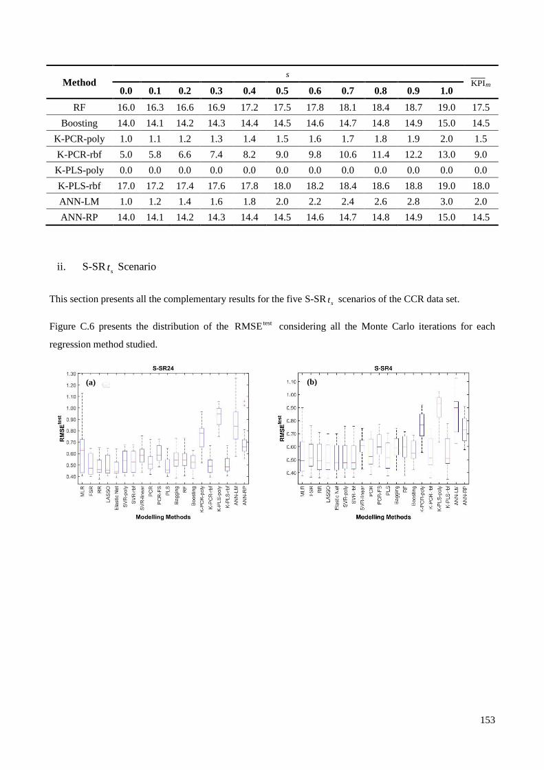
153
Method s
KPIm 0.0 0.1 0.2 0.3 0.4 0.5 0.6 0.7 0.8 0.9 1.0
RF 16.0 16.3 16.6 16.9 17.2 17.5 17.8 18.1 18.4 18.7 19.0 17.5
Boosting 14.0 14.1 14.2 14.3 14.4 14.5 14.6 14.7 14.8 14.9 15.0 14.5
K-PCR-poly 1.0 1.1 1.2 1.3 1.4 1.5 1.6 1.7 1.8 1.9 2.0 1.5
K-PCR-rbf 5.0 5.8 6.6 7.4 8.2 9.0 9.8 10.6 11.4 12.2 13.0 9.0
K-PLS-poly 0.0 0.0 0.0 0.0 0.0 0.0 0.0 0.0 0.0 0.0 0.0 0.0
K-PLS-rbf 17.0 17.2 17.4 17.6 17.8 18.0 18.2 18.4 18.6 18.8 19.0 18.0
ANN-LM 1.0 1.2 1.4 1.6 1.8 2.0 2.2 2.4 2.6 2.8 3.0 2.0
ANN-RP 14.0 14.1 14.2 14.3 14.4 14.5 14.6 14.7 14.8 14.9 15.0 14.5
ii. S-SRst Scenario
This section presents all the complementary results for the five S-SRst scenarios of the CCR data set.
Figure C.6 presents the distribution of the testRMSE considering all the Monte Carlo iterations for each
regression method studied.
(b) (a)

154
Figure C.6 Box plot of the testRMSE , for the CCR data set, considering all the considering all Monte Carlo iterations for each
regression method used for all the S-SR st scenarios: (a) S-SR24: (b) S-SR4; (c) S-SR3; (d) S-SR2; (e) S-SR1.
Figure C.7 presents the results of the pairwise student’s -testt for all the synchronized scenarios.
(c) (d)
(e)
(a) (b)

155
Figure C.7 Heatmap results of the pairwise student’s t -test, for the CCR data set, considering all the considering all Monte Carlo
iterations for each regression method used for all the S-SR st scenarios: (a) S-SR24: (b) S-SR4; (c) S-SR3; (d) S-SR2; (e) S-SR1. A
green colour indicates that the method indicated in the Y-axis is better in a statistically significant sense, over the corresponding method
indicated in the X-axis. A yellow colour indicates that no statistically significant different exists between the methods.
Table C.9 presents the ( )KPI s values depending on the “draw” score, for the calculation of the Mean KPI and
Mean Rank present in Equations (5.2) and (5.3) for the S-SR24 scenario.
Table C.9 Results of the ( )KPI s for the S-SR24 scenario for the CCR data set.
Method s
KPIm 0.0 0.1 0.2 0.3 0.4 0.5 0.6 0.7 0.8 0.9 1.0
MLR 3.0 3.6 4.2 4.8 5.4 6.0 6.6 7.2 7.8 8.4 9.0 6.0
FSR 12.0 12.6 13.2 13.8 14.4 15.0 15.6 16.2 16.8 17.4 18.0 15.0
RR 15.0 15.3 15.6 15.9 16.2 16.5 16.8 17.1 17.4 17.7 18.0 16.5
LASSO 15.0 15.4 15.8 16.2 16.6 17.0 17.4 17.8 18.2 18.6 19.0 17.0
EN 18.0 18.1 18.2 18.3 18.4 18.5 18.6 18.7 18.8 18.9 19.0 18.5
SVR-poly 7.0 7.7 8.4 9.1 9.8 10.5 11.2 11.9 12.6 13.3 14.0 10.5
SVR-rbf 7.0 7.7 8.4 9.1 9.8 10.5 11.2 11.9 12.6 13.3 14.0 10.5
SVR-linear 4.0 4.2 4.4 4.6 4.8 5.0 5.2 5.4 5.6 5.8 6.0 5.0
PCR 6.0 6.6 7.2 7.8 8.4 9.0 9.6 10.2 10.8 11.4 12.0 9.0
(e)
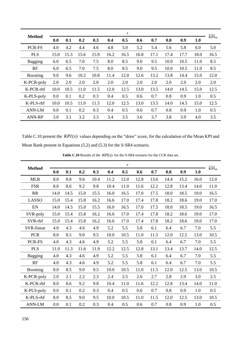
156
Method s
KPIm 0.0 0.1 0.2 0.3 0.4 0.5 0.6 0.7 0.8 0.9 1.0
PCR-FS 4.0 4.2 4.4 4.6 4.8 5.0 5.2 5.4 5.6 5.8 6.0 5.0
PLS 15.0 15.3 15.6 15.9 16.2 16.5 16.8 17.1 17.4 17.7 18.0 16.5
Bagging 6.0 6.5 7.0 7.5 8.0 8.5 9.0 9.5 10.0 10.5 11.0 8.5
RF 6.0 6.5 7.0 7.5 8.0 8.5 9.0 9.5 10.0 10.5 11.0 8.5
Boosting 9.0 9.6 10.2 10.8 11.4 12.0 12.6 13.2 13.8 14.4 15.0 12.0
K-PCR-poly 2.0 2.0 2.0 2.0 2.0 2.0 2.0 2.0 2.0 2.0 2.0 2.0
K-PCR-rbf 10.0 10.5 11.0 11.5 12.0 12.5 13.0 13.5 14.0 14.5 15.0 12.5
K-PLS-poly 0.0 0.1 0.2 0.3 0.4 0.5 0.6 0.7 0.8 0.9 1.0 0.5
K-PLS-rbf 10.0 10.5 11.0 11.5 12.0 12.5 13.0 13.5 14.0 14.5 15.0 12.5
ANN-LM 0.0 0.1 0.2 0.3 0.4 0.5 0.6 0.7 0.8 0.9 1.0 0.5
ANN-RP 3.0 3.1 3.2 3.3 3.4 3.5 3.6 3.7 3.8 3.9 4.0 3.5
Table C.10 present the ( )KPI s values depending on the “draw” score, for the calculation of the Mean KPI and
Mean Rank present in Equations (5.2) and (5.3) for the S-SR4 scenario.
Table C.10 Results of the ( )KPI s for the S-SR4 scenario for the CCR data set.
Method s
KPIm 0.0 0.1 0.2 0.3 0.4 0.5 0.6 0.7 0.8 0.9 1.0
MLR 8.0 8.8 9.6 10.4 11.2 12.0 12.8 13.6 14.4 15.2 16.0 12.0
FSR 8.0 8.6 9.2 9.8 10.4 11.0 11.6 12.2 12.8 13.4 14.0 11.0
RR 14.0 14.5 15.0 15.5 16.0 16.5 17.0 17.5 18.0 18.5 19.0 16.5
LASSO 15.0 15.4 15.8 16.2 16.6 17.0 17.4 17.8 18.2 18.6 19.0 17.0
EN 14.0 14.5 15.0 15.5 16.0 16.5 17.0 17.5 18.0 18.5 19.0 16.5
SVR-poly 15.0 15.4 15.8 16.2 16.6 17.0 17.4 17.8 18.2 18.6 19.0 17.0
SVR-rbf 15.0 15.4 15.8 16.2 16.6 17.0 17.4 17.8 18.2 18.6 19.0 17.0
SVR-linear 4.0 4.3 4.6 4.9 5.2 5.5 5.8 6.1 6.4 6.7 7.0 5.5
PCR 8.0 8.5 9.0 9.5 10.0 10.5 11.0 11.5 12.0 12.5 13.0 10.5
PCR-FS 4.0 4.3 4.6 4.9 5.2 5.5 5.8 6.1 6.4 6.7 7.0 5.5
PLS 11.0 11.3 11.6 11.9 12.2 12.5 12.8 13.1 13.4 13.7 14.0 12.5
Bagging 4.0 4.3 4.6 4.9 5.2 5.5 5.8 6.1 6.4 6.7 7.0 5.5
RF 4.0 4.3 4.6 4.9 5.2 5.5 5.8 6.1 6.4 6.7 7.0 5.5
Boosting 8.0 8.5 9.0 9.5 10.0 10.5 11.0 11.5 12.0 12.5 13.0 10.5
K-PCR-poly 2.0 2.1 2.2 2.3 2.4 2.5 2.6 2.7 2.8 2.9 3.0 2.5
K-PCR-rbf 8.0 8.6 9.2 9.8 10.4 11.0 11.6 12.2 12.8 13.4 14.0 11.0
K-PLS-poly 0.0 0.1 0.2 0.3 0.4 0.5 0.6 0.7 0.8 0.9 1.0 0.5
K-PLS-rbf 8.0 8.5 9.0 9.5 10.0 10.5 11.0 11.5 12.0 12.5 13.0 10.5
ANN-LM 0.0 0.1 0.2 0.3 0.4 0.5 0.6 0.7 0.8 0.9 1.0 0.5

157
Method s
KPIm 0.0 0.1 0.2 0.3 0.4 0.5 0.6 0.7 0.8 0.9 1.0
ANN-RP 2.0 2.1 2.2 2.3 2.4 2.5 2.6 2.7 2.8 2.9 3.0 2.5
Table C.11 presents the ( )KPI s values depending on the “draw” score, for the calculation of the Mean KPI
and Mean Rank present in Equations (5.2) and (5.3) for the S-SR3 scenario.
Table C.11 Results of the ( )KPI s for the S-SR3 scenario for the CCR data set.
Method s
KPIm 0.0 0.1 0.2 0.3 0.4 0.5 0.6 0.7 0.8 0.9 1.0
MLR 2.0 2.5 3.0 3.5 4.0 4.5 5.0 5.5 6.0 6.5 7.0 4.5
FSR 6.0 7.0 8.0 9.0 10.0 11.0 12.0 13.0 14.0 15.0 16.0 11.0
RR 5.0 6.3 7.6 8.9 10.2 11.5 12.8 14.1 15.4 16.7 18.0 11.5
LASSO 16.0 16.2 16.4 16.6 16.8 17.0 17.2 17.4 17.6 17.8 18.0 17.0
EN 19.0 19.0 19.0 19.0 19.0 19.0 19.0 19.0 19.0 19.0 19.0 19.0
SVR-poly 6.0 7.1 8.2 9.3 10.4 11.5 12.6 13.7 14.8 15.9 17.0 11.5
SVR-rbf 6.0 7.1 8.2 9.3 10.4 11.5 12.6 13.7 14.8 15.9 17.0 11.5
SVR-linear 5.0 6.0 7.0 8.0 9.0 10.0 11.0 12.0 13.0 14.0 15.0 10.0
PCR 7.0 7.9 8.8 9.7 10.6 11.5 12.4 13.3 14.2 15.1 16.0 11.5
PCR-FS 4.0 4.2 4.4 4.6 4.8 5.0 5.2 5.4 5.6 5.8 6.0 5.0
PLS 14.0 14.4 14.8 15.2 15.6 16.0 16.4 16.8 17.2 17.6 18.0 16.0
Bagging 6.0 6.9 7.8 8.7 9.6 10.5 11.4 12.3 13.2 14.1 15.0 10.5
RF 5.0 5.8 6.6 7.4 8.2 9.0 9.8 10.6 11.4 12.2 13.0 9.0
Boosting 7.0 7.9 8.8 9.7 10.6 11.5 12.4 13.3 14.2 15.1 16.0 11.5
K-PCR-poly 2.0 2.2 2.4 2.6 2.8 3.0 3.2 3.4 3.6 3.8 4.0 3.0
K-PCR-rbf 9.0 9.7 10.4 11.1 11.8 12.5 13.2 13.9 14.6 15.3 16.0 12.5
K-PLS-poly 0.0 0.0 0.0 0.0 0.0 0.0 0.0 0.0 0.0 0.0 0.0 0.0
K-PLS-rbf 6.0 7.0 8.0 9.0 10.0 11.0 12.0 13.0 14.0 15.0 16.0 11.0
ANN-LM 1.0 1.0 1.0 1.0 1.0 1.0 1.0 1.0 1.0 1.0 1.0 1.0
ANN-RP 2.0 2.2 2.4 2.6 2.8 3.0 3.2 3.4 3.6 3.8 4.0 3.0
Table C.12 presents the ( )KPI s values depending on the “draw” score, for the calculation of the Mean KPI
and Mean Rank present in Equations (5.2) and (5.3) for the S-SR2 scenario.
Table C.12 Results of the ( )KPI s for the S-SR2 scenario for the CCR data set.
Method s
KPIm 0.0 0.1 0.2 0.3 0.4 0.5 0.6 0.7 0.8 0.9 1.0
MLR 1.0 2.2 3.4 4.6 5.8 7.0 8.2 9.4 10.6 11.8 13.0 7.0

158
Method s
KPIm 0.0 0.1 0.2 0.3 0.4 0.5 0.6 0.7 0.8 0.9 1.0
FSR 4.0 5.1 6.2 7.3 8.4 9.5 10.6 11.7 12.8 13.9 15.0 9.5
RR 3.0 4.6 6.2 7.8 9.4 11.0 12.6 14.2 15.8 17.4 19.0 11.0
LASSO 14.0 14.5 15.0 15.5 16.0 16.5 17.0 17.5 18.0 18.5 19.0 16.5
EN 15.0 15.4 15.8 16.2 16.6 17.0 17.4 17.8 18.2 18.6 19.0 17.0
SVR-poly 5.0 6.1 7.2 8.3 9.4 10.5 11.6 12.7 13.8 14.9 16.0 10.5
SVR-rbf 6.0 7.0 8.0 9.0 10.0 11.0 12.0 13.0 14.0 15.0 16.0 11.0
SVR-linear 6.0 6.9 7.8 8.7 9.6 10.5 11.4 12.3 13.2 14.1 15.0 10.5
PCR 6.0 6.9 7.8 8.7 9.6 10.5 11.4 12.3 13.2 14.1 15.0 10.5
PCR-FS 3.0 3.5 4.0 4.5 5.0 5.5 6.0 6.5 7.0 7.5 8.0 5.5
PLS 14.0 14.5 15.0 15.5 16.0 16.5 17.0 17.5 18.0 18.5 19.0 16.5
Bagging 5.0 5.7 6.4 7.1 7.8 8.5 9.2 9.9 10.6 11.3 12.0 8.5
RF 5.0 5.9 6.8 7.7 8.6 9.5 10.4 11.3 12.2 13.1 14.0 9.5
Boosting 7.0 8.0 9.0 10.0 11.0 12.0 13.0 14.0 15.0 16.0 17.0 12.0
K-PCR-poly 1.0 1.3 1.6 1.9 2.2 2.5 2.8 3.1 3.4 3.7 4.0 2.5
K-PCR-rbf 13.0 13.6 14.2 14.8 15.4 16.0 16.6 17.2 17.8 18.4 19.0 16.0
K-PLS-poly 0.0 0.0 0.0 0.0 0.0 0.0 0.0 0.0 0.0 0.0 0.0 0.0
K-PLS-rbf 5.0 6.0 7.0 8.0 9.0 10.0 11.0 12.0 13.0 14.0 15.0 10.0
ANN-LM 1.0 1.3 1.6 1.9 2.2 2.5 2.8 3.1 3.4 3.7 4.0 2.5
ANN-RP 1.0 1.5 2.0 2.5 3.0 3.5 4.0 4.5 5.0 5.5 6.0 3.5
Table C.13 presents the ( )KPI s values depending on the “draw” score, for the calculation of the Mean KPI
and Mean Rank present in Equations (5.2) and (5.3) for the S-SR1 scenario.
Table C.13 Results of the ( )KPI s for the S-SR1 scenario for the CCR data set.
Method s
KPIm 0.0 0.1 0.2 0.3 0.4 0.5 0.6 0.7 0.8 0.9 1.0
MLR 2.0 3.0 4.0 5.0 6.0 7.0 8.0 9.0 10.0 11.0 12.0 7.0
FSR 4.0 4.8 5.6 6.4 7.2 8.0 8.8 9.6 10.4 11.2 12.0 8.0
RR 18.0 18.1 18.2 18.3 18.4 18.5 18.6 18.7 18.8 18.9 19.0 18.5
LASSO 12.0 12.4 12.8 13.2 13.6 14.0 14.4 14.8 15.2 15.6 16.0 14.0
EN 13.0 13.5 14.0 14.5 15.0 15.5 16.0 16.5 17.0 17.5 18.0 15.5
SVR-poly 10.0 10.8 11.6 12.4 13.2 14.0 14.8 15.6 16.4 17.2 18.0 14.0
SVR-rbf 10.0 10.8 11.6 12.4 13.2 14.0 14.8 15.6 16.4 17.2 18.0 14.0
SVR-linear 5.0 5.4 5.8 6.2 6.6 7.0 7.4 7.8 8.2 8.6 9.0 7.0
PCR 8.0 8.6 9.2 9.8 10.4 11.0 11.6 12.2 12.8 13.4 14.0 11.0
PCR-FS 4.0 4.3 4.6 4.9 5.2 5.5 5.8 6.1 6.4 6.7 7.0 5.5
PLS 14.0 14.4 14.8 15.2 15.6 16.0 16.4 16.8 17.2 17.6 18.0 16.0

159
Method s
KPIm 0.0 0.1 0.2 0.3 0.4 0.5 0.6 0.7 0.8 0.9 1.0
Bagging 4.0 4.4 4.8 5.2 5.6 6.0 6.4 6.8 7.2 7.6 8.0 6.0
RF 6.0 6.3 6.6 6.9 7.2 7.5 7.8 8.1 8.4 8.7 9.0 7.5
Boosting 8.0 8.6 9.2 9.8 10.4 11.0 11.6 12.2 12.8 13.4 14.0 11.0
K-PCR-poly 2.0 2.2 2.4 2.6 2.8 3.0 3.2 3.4 3.6 3.8 4.0 3.0
K-PCR-rbf 12.0 12.5 13.0 13.5 14.0 14.5 15.0 15.5 16.0 16.5 17.0 14.5
K-PLS-poly 0.0 0.1 0.2 0.3 0.4 0.5 0.6 0.7 0.8 0.9 1.0 0.5
K-PLS-rbf 8.0 9.1 10.2 11.3 12.4 13.5 14.6 15.7 16.8 17.9 19.0 13.5
ANN-LM 0.0 0.1 0.2 0.3 0.4 0.5 0.6 0.7 0.8 0.9 1.0 0.5
ANN-RP 2.0 2.2 2.4 2.6 2.8 3.0 3.2 3.4 3.6 3.8 4.0 3.0
iii. S-SR1L2 Scenario
This section presents all the complementary results for the S-SR1L2 scenario of the CCR data set.
Figure C.8 presents the distribution of the testRMSE considering all the Monte Carlo iterations for each
regression method studied.
Figure C.8 Box plot of the testRMSE , for the S-SR1L2 scenario for the CCR data set, considering all the considering all Monte Carlo
iterations for each regression method used.
Table C.14 presents the ( )KPI s values depending on the “draw” score, for the calculation of the Mean KPI
and Mean Rank present in Equations (5.2) and (5.3) for the S-SR1L2 scenario.
Table C.14 Results of the ( )KPI s for the S-SR1L2 scenario for the CCR data set.
Method s
KPIm 0.0 0.1 0.2 0.3 0.4 0.5 0.6 0.7 0.8 0.9 1.0
MLR 0.0 0.2 0.4 0.6 0.8 1.0 1.2 1.4 1.6 1.8 2.0 1.0
FSR 5.0 5.6 6.2 6.8 7.4 8.0 8.6 9.2 9.8 10.4 11.0 8.0
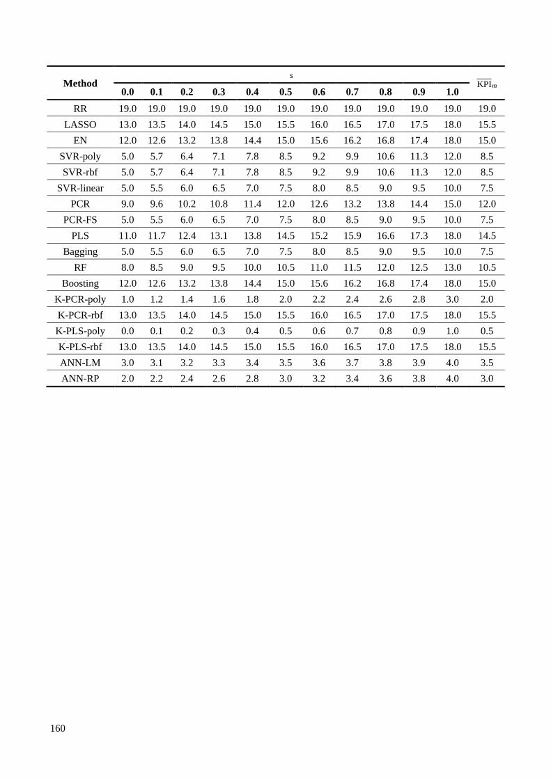
160
Method s
KPIm 0.0 0.1 0.2 0.3 0.4 0.5 0.6 0.7 0.8 0.9 1.0
RR 19.0 19.0 19.0 19.0 19.0 19.0 19.0 19.0 19.0 19.0 19.0 19.0
LASSO 13.0 13.5 14.0 14.5 15.0 15.5 16.0 16.5 17.0 17.5 18.0 15.5
EN 12.0 12.6 13.2 13.8 14.4 15.0 15.6 16.2 16.8 17.4 18.0 15.0
SVR-poly 5.0 5.7 6.4 7.1 7.8 8.5 9.2 9.9 10.6 11.3 12.0 8.5
SVR-rbf 5.0 5.7 6.4 7.1 7.8 8.5 9.2 9.9 10.6 11.3 12.0 8.5
SVR-linear 5.0 5.5 6.0 6.5 7.0 7.5 8.0 8.5 9.0 9.5 10.0 7.5
PCR 9.0 9.6 10.2 10.8 11.4 12.0 12.6 13.2 13.8 14.4 15.0 12.0
PCR-FS 5.0 5.5 6.0 6.5 7.0 7.5 8.0 8.5 9.0 9.5 10.0 7.5
PLS 11.0 11.7 12.4 13.1 13.8 14.5 15.2 15.9 16.6 17.3 18.0 14.5
Bagging 5.0 5.5 6.0 6.5 7.0 7.5 8.0 8.5 9.0 9.5 10.0 7.5
RF 8.0 8.5 9.0 9.5 10.0 10.5 11.0 11.5 12.0 12.5 13.0 10.5
Boosting 12.0 12.6 13.2 13.8 14.4 15.0 15.6 16.2 16.8 17.4 18.0 15.0
K-PCR-poly 1.0 1.2 1.4 1.6 1.8 2.0 2.2 2.4 2.6 2.8 3.0 2.0
K-PCR-rbf 13.0 13.5 14.0 14.5 15.0 15.5 16.0 16.5 17.0 17.5 18.0 15.5
K-PLS-poly 0.0 0.1 0.2 0.3 0.4 0.5 0.6 0.7 0.8 0.9 1.0 0.5
K-PLS-rbf 13.0 13.5 14.0 14.5 15.0 15.5 16.0 16.5 17.0 17.5 18.0 15.5
ANN-LM 3.0 3.1 3.2 3.3 3.4 3.5 3.6 3.7 3.8 3.9 4.0 3.5
ANN-RP 2.0 2.2 2.4 2.6 2.8 3.0 3.2 3.4 3.6 3.8 4.0 3.0