LINKAGES BETWEEN THE GAUSS MAP AND THE STERN-BROCOT TREE

Acta Mathematica Academiae Paedagogicae Nyıregyhaziensis22 (2006), 217–235www.emis.de/journals

ISSN 1786-0091

LINKAGES BETWEEN THE GAUSS MAP AND THESTERN-BROCOT TREE

BRUCE BATES, MARTIN BUNDER, AND KEITH TOGNETTI

Abstract. We discover a bijective map between the Gauss Map and theleft-half of the Stern-Brocot Tree. The domain of the Gauss Map is thenextended to cover all reals, and the coverage of the Stern-Brocot Tree isextended to include all positive and negative rationals in a manner thatpreserves the map between the two constructions.

1. Introduction

That the Gauss Map and the Stern-Brocot Tree have corresponding fea-tures seems, at first glance, unintuitive. The Stern-Brocot Tree is a number-theoretic construction built on a strange algebra (child’s addition) that seemsfar removed from a locally differentiable function based on the function 1

x. Yet

nonetheless, there are interesting areas of correspondence. We begin with theGauss Map, which we define based on the notation in Corless [2].

Definition 1 (Gauss Map). The Gauss Map, G (x) is defined as

G (x) =

{1x

mod 1 = frac 1x, for x ∈ (0, 1]

0, for x = 0.

The Gauss Map and its iterates are made up of disjoint continuous parts.The following definition of these parts is a variation of the notation found inBates et al [1].

Definition 2 (Parts in the Gauss Map). [0; j1, . . . , jk] is that part of Gk whosedomain is

[{0; j1, . . . , jk}, {0; j1, . . . , jk, 1})if k is even, and

({0; j1, . . . , jk, 1}, {0; j1, . . . , jk}]if k is odd.

2000 Mathematics Subject Classification. 11A55, 05C05.Key words and phrases. Gauss Map, Stern-Brocot Tree.

217

218 BRUCE BATES, MARTIN BUNDER, AND KEITH TOGNETTI

The points of discontinuity in the kth iterate, Gk, of the Gauss Map are{x : Gk (x) = 0}. Accordingly, the set of points of discontinuity in the domainof G is

(1.1)

{1,

1

2,1

3,1

4, . . .

}.

In continued fraction notation, these same points of discontinuity are values ofx that increment by one in the last entry of their continued fraction expansion.Thus within G, the set (1.1) in continued fraction notation becomes:

{{0; 1} , {0; 2}, {0; 3}, {0; 4}, . . .} .

In general, [0; j1, . . . , jk] is discontinuous with the rest of Gkat {0; j1, . . . , jk}and {0; j1, . . . , jk, 1}. Note that there is no part defined at the origin.

From hereon, where there is no ambiguity, we refer to the Gauss Map andits iterates as simply the Gauss Map.

2. Clusters within the Gauss Map

Definition 3 (Clusters). A cluster within Gk is an infinite set of consecutiveparts of Gk whose slopes become progressively more vertical and approachinfinity in their limit. The cluster is bounded by a line with vertical slopecalled the cluster line. This bound is not part of the cluster.

Example 1. G is made up of the elements of a single cluster whose cluster lineis x = 0.

Theorem 1. The set of consecutive parts [0; j1, . . . , jk, 1] , [0; j1, . . . , jk, 2] , . . .forms a cluster in Gk+1 with cluster line x = {0; j1, . . . , jk}.Proof. For k odd, the union of the set of consecutive parts

[0; j1, . . . , jk, 1] , [0; j1, . . . , jk, 2] , [0; j1, . . . , jk, 3] , . . .

has least upper and greatest lower bounds {0; j1, . . . , jk} = pk

qkand

{0; j1, . . . , jk, 1} =pk + pk−1

qk + qk−1

respectively. For k even the bounds are reversed.We have shown in [1] that, if x ∈ ({0; j1, . . . , jk+1}, {0; j1, . . . , jk+1 + 1}) ,

Gk+1(x) =qk+1x− pk+1

pk − qkx

where pk

qk= {0; j1, . . . , jk} and pk+1

qk+1= {0; j1, . . . , jk+1}.

Sinced

dxGk+1 (x) =

pkqk+1 − pk+1qk

(pk − qkx)2

=(−1)k+1

(pk − qkx)2

LINKAGES BETWEEN THE GAUSS MAP AND THE STERN-BROCOT TREE 219

→ ±∞ as x → pk

qk

it follows that each consecutive part in the set

[0; j1, . . . , jk, 1] , [0; j1, . . . , jk, 2] , . . .

becomes progressively more vertical. The vertical line x = pk

qk= {0; j1, . . . , jk}

lies outside the set but is the limit of the set. Thus by Definition 3 the infiniteset of consecutive parts [0; j1, . . . , jk, 1], [0; j1, . . . , jk, 2] , . . . forms a cluster inGk+1 with cluster line x = {0; j1, . . . , jk}. ¤

We denote the cluster

[0; j1, . . . , jk, 1] , [0; j1, . . . , jk, 2] , . . .

in Gk+1 by 〈〈0, j1, . . . , jk, 〉〉. The cluster in G is 〈〈0〉〉 and represents the entirefirst iterate.

Definition 4 (Domains and Open Domains of Sets). Let the domain of eachfunction in a set of functions be known. Then the union of the domainsof each function in the set is called the domain of the set. The domain of afunction minus its endpoints (if any) is called the open domain of the function.Similarly, the domain of a set minus its endpoints (if any) is called the opendomain of the set.

For simplicity, let the interval (a, b), where a < b, be equivalently representedby (b, a). It follows from Definition 4 that:

i) The domain of a cluster is the union of the domains of each part in thecluster.

ii) The open domain of [0; j1, . . . , jk, t] is the interval

({0; j1, . . . , jk, t} , {0; j1, . . . , jk, t + 1}) .

Theorem 2. The open domain of the part [0; j1, . . . , jk] in Gk is the opendomain of the cluster 〈〈0, j1, . . . , jk〉〉 in Gk+1.

Proof. The open domain of [0; j1, . . . , jk] in Gk is

({0; j1, . . . , jk} , {0; j1, . . . , jk, 1}) .

Consider any two consecutive parts [0; j1, . . . , jk, t] and [0; j1, . . . , jk, t + 1] inthe cluster 〈〈0, j1, . . . , jk〉〉 in Gk+1. By Definition 2, [0; j1, . . . , jk, t] has domain

[{0; j1, . . . , jk, t} , {0; j1, . . . , jk, t + 1})for k even and

({0; j1, . . . , jk, t + 1} , {0; j1, . . . , jk, t}]for k odd.

Similarly, [0; j1, . . . , jk, t + 1] has domain

[{0; j1, . . . , jk, t + 1} , {0; j1, . . . , jk, t + 2})


for k even and

({0; j1, . . . , jk, t + 2} , {0; j1, . . . , jk, t + 1}]for k odd. It follows that the domain of the set of two consecutive parts in〈〈0, j1, . . . , jk〉〉 is continuous and non-overlapping. Therefore the domain ofthe cluster 〈〈0, j1, . . . , jk〉〉 is continuous and non-overlapping. Accordingly,the only endpoints of 〈〈0, j1, . . . , jk〉〉 are {0; j1, . . . , jk} and {0; j1, . . . , jk, 1},and its open domain is

({0; j1, . . . , jk} , {0; j1, . . . , jk, 1}) ,

establishing our theorem. ¤

Corollary 1. The only clusters within Gk+1 are those of the form

〈〈0, j1, . . . , jk〉〉where the open domain of 〈〈0, j1, . . . , jk〉〉 is the open domain of [0; j1, . . . , jk]in Gk.

Proof. G (x) = 〈〈0〉〉 and represents a single cluster with open domain (0, 1).By Theorem 2, G2 (x) consists entirely of clusters of the form 〈〈0, j1〉〉 wherethe open domain of 〈〈0, j1〉〉 is the open domain of [0; j1] in G. RepeatingTheorem 2 for G3, G4, . . . establishes our corollary. ¤

Since from the proof of Theorem 1, ddx

Gk (x) = (−1)k

(pk−1−qk−1x)2, it follows that

within Gk, parts have negative slope for k odd and positive slope for k even.

Summary 1. The following is a summary of important characteristics of theGauss Map:

1. Every part of the Gauss Map belongs to a cluster.2. Each cluster has an infinite number of parts.3. All parts within odd iterates have negative slope; all parts within even

iterates have positive slope.4. The slopes of successive parts within a cluster become progressively

steeper.5. The cluster line is vertical and is not part of the cluster.6. Clusters within Gk+1 are all of the form 〈〈0, j1, . . . , jk〉〉 where the open

domain of 〈〈0, j1, . . . , jk〉〉 is the open domain of the part [0; j1, . . . , jk] in Gk.

3. Terms in the Stern-Brocot Tree

Let the level of the Stern-Brocot Tree consisting of the terms 01

and 10

becalled Level 0. Except for terms in level 0, each term of the Stern-Brocot Treeis the mediant of two terms, called parents, found in lower ordinal levels of thetree. The following definitions formalise our understanding of entries in eachlevel of the tree


Definition 5 (Mediant). If m, n, s, t are integers then the mediant of mn

andst, written as m

n+ s

tis m+s

n+t.The operation + is called child’s addition.

Definition 6 (Interleave Operator). We denote by #, the interleave operatoracting on two ordered sets A = 〈a1, a2, . . . , ak+1〉 and B = 〈b1, b2, . . . , bk〉 , suchthat A#B = C where C = 〈a1, b1, a2, b2, . . . , bk, ak+1〉 .

Definition 7 (Stern-Brocot Sequence). Let H0 =⟨

01, 1

0

⟩and for k ≥ 1,

Hk = Hk−1# med Hk−1

where med Hk−1 denotes the increasing sequence of mediants that are gener-ated from consecutive terms in Hk−1.

That is, ifHk−1 =

⟨hk−1,1, hk−1,2, . . . , hk−1,2k+1

⟩

then

med Hk−1 =⟨(hk−1,1 + hk−1,2) , (hk−1,2 + hk−1,3) , . . . ,

(hk−1,2k + hk−1,2k+1

)⟩.

Hk represents the increasing sequence containing both the first k generations ofmediants based on H0, and the terms of H0 itself. It is styled the Stern-Brocotsequence.

Definition 8 (Stern-Brocot Tree). The Stern-Brocot Tree is a series of levelsgiven by:

Level 0 01

10

Level 1 med H0

Level 2 med H1

Level 3 med H2...

...

The right half of Figure 1 (with the inclusion of the term 01) represents the

first five levels of the Stern-Brocot Tree.

We can uniquely locate any term in the tree by introducing Right-Left no-tation. Consider the term 8

11. We locate 8

11by moving from level 0, one level

at a time, through successive mediants. Thus beginning at 01, we move to the

right and down to 11, to the left and down to 1

2, to the right and down to 2

3, to

the right and down to 34, to the left and down to 5

7and finally to the right and

down to 811

. It is obvious that this is the only route by which we can move

from 01

to 811

, traversing one level at a time and one successive mediant at atime. Generalising for the tree, every term can be uniquely located in the treeby a succession of these right or left and down moves. Thus our Right-Leftnotation is a handy way of describing any term in the tree. In our examplewe adopt the notation RLR2LR to represent 8

11. This denotes that we move

from 01

to the right and down once, then to the left and down once, then tothe right and down twice, then to the left and down once and finally to theright and down once to arrive at 8

11.


Based on Graham et al [3], it can be easily shown that, for a0 ≥ 0, a1 ≥1, a2 ≥ 1, . . . , ak ≥ 1,

(3.1) {a0; a1, a2, . . . , ak + 1} =

{Ra0+1La1Ra2 . . . Lak for k oddRa0+1La1Ra2 . . . Rak for k even

where the left hand side of (3.1) is the continued fraction expansion of theterm represented by the right hand side of (3.1). Thus 8

11= {0; 1, 2, 1, 2} =

R1LR2LR. Note that we have chosen a variation on the notation found in [3].Graham et al do not commence the right and left movements from 0

1because

the first movement to 11

is common to all entries in the tree and can be ignored

by defining that all movements commence from 11. However we later extend

the Stern-Brocot Tree to include negative fractions. In order to locate entriesin this extended tree, and thereby generalise the process for all fractions, thescheme of right and left movements needs to begin at 0

1.

4. Branches in the Stern-Brocot Tree

We now introduce branches within the Stern-Brocot Tree as a prelude todiscovering their linkage to clusters in the Gauss Map. Firstly, we categorisemediants according to the following definition:

Definition 9 (Left and Right Mediants). A left (right) mediant is the mediantformed in level k + 1 that is smaller (greater) than its parent found in level k.

Definition 10 (Left and Right Branches). The set of all mediants possessinga common parent µ and whose elements are smaller than µ is called the leftbranch of µ; the set of all mediants possessing a common parent µ and whoseelements are greater than µ is called the right branch of µ.

Definition 10 can be alternatively stated as follows: Let µ be a term in theStern-Brocot Tree and µl its left mediant. The left branch of µ is the setconsisting of µl and all successive right mediants of µl. Similarly, let µr bethe right mediant of µ. The right branch of µ is the set consisting of µr andall successive left mediants of µr. It follows from Definition 10 that each termordinally above level 0 in the tree belongs to two branches - the left branch ofone parent and the right branch of the other parent.

We can represent each rational number by a terminating continued fractionthat has a short and a long form. Thus for a0 ≥ 0, a1 ≥ 1, a2 ≥ 1, . . . , ak > 1,we have {a0; a1, a2, . . . , ak} = {a0; a1, a2, . . . , ak − 1, 1} where the continuedfraction on the left is the short form and the continued fraction on the right isthe long form. The following theorem links branches and the short and longform of terms in the Stern-Brocot Tree. It shows that the left and right branchof a term is built upon the short and long form of the term.

Theorem 3. Let {a0; a1, a2, . . . , ak} be the short form of µ. Then


i) for k odd, the right branch of µ is the set

{{a0; a1, a2, . . . , ak − 1, 1, t} | t ≥ 1}and the left branch of µ is the set

{{a0; a1, a2, . . . , ak, t} | t ≥ 1} ;

ii) for k even, the right branch of µ is the set

{{a0; a1, a2, . . . , ak, t} | t ≥ 1}and the left branch of µ is the set

{{a0; a1, a2, . . . , ak − 1, 1, t} | t ≥ 1} .

Proof. From (3.1), let µ = Ra0+1La1Ra2 . . . Lak−1 = {a0; a1, a2, . . . , ak} wherek is odd. Then

µl = Ra0+1La1Ra2 . . . Lak = {a0; a1, a2, . . . , ak + 1} = {a0; a1, a2, . . . , ak, 1}and the left branch of µ is the set{

Ra0+1La1Ra2 . . . LakRt | t ≥ 0}

= {{a0; a1, a2, . . . , ak, t} | t ≥ 1} .

Similarly, from (3.1),

µr = Ra0+1La1Ra2 . . . Lak−1R = {a0; a1, a2, . . . , ak − 1, 2}= {a0; a1, a2, . . . , ak − 1, 1, 1}

and the right branch of µ is the set{Ra0+1La1Ra2 . . . LakRLt | t ≥ 0

}= {{a0; a1, a2, . . . , ak − 1, 1, t} | t ≥ 1} .

The case for k even, follows the same reasoning as that for k odd. ¤Corollary 2. Left (right) mediants have an even (odd) number of terms intheir continued fraction expansions.

Proof. From Theorem 3, let {a0; a1, a2, . . . , ak} be the short form of µ. Theni) for k odd, the right mediant of µ is

{a0; a1, a2, . . . , ak − 1, 1, 1} = {a0; a1, a2, . . . , ak − 1, 2}and the left mediant of µ is

{a0; a1, a2, . . . , ak, 1} = {a0; a1, a2, . . . , ak + 1} ;

ii) for k even, the right mediant of µ is

{a0; a1, a2, . . . , ak, 1} = {a0; a1, a2, . . . , ak + 1}and the left mediant of µ is

{a0; a1, a2, . . . , ak − 1, 1, 1} = {a0; a1, a2, . . . , ak − 1, 2} .

¤


We call µ in Theorem 3 the pivot of the two branches that are described inthe theorem. Clearly every term in the tree except 0

1and 1

0is a pivot for a

left branch and a right branch. (01

is a pivot only for a right branch but no

left branch; and 10

is defined as the pivot for the left branch{

11, 2

1, 3

1, . . .

}. 1

0

is not a pivot for any right branch). Theorem 3 shows that every branch ofthe Stern-Brocot Tree possesses members whose continued fraction expansionsare identical except in their last terms. Their last terms increment as wemove down the branch. Thus if a branch has k terms in the continued fractionexpansion of its members, the first k−1 terms are common for every member ofthe branch and correspond to the short or long form of the continued fractionexpansion of the pivot.

Definition 11 (Continued Fraction Notation for a Branch). The branch inthe Stern-Brocot Tree consisting of all continued fractions of the form

{0; j1, j2, . . . , jk, t}where t = 1, 2, 3, . . . , is denoted by

−−−−−−−−−−−→{0, j1, j2, . . . , jk} and its extended branchconsists of all continued fractions of the form {0; j1, j2, . . . , jk, t} where t =

0, 1, 2, . . . , is denoted by ˜{0, j1, j2, . . . , jk}. The domain of a branch consists ofall reals that lie between the first term of the branch and its pivot.

We note that an extended branch is formed when the parent of the first termof a branch that is not the pivot of the branch, is added to the branch.

Example 2. The right branch−→{0} = {1

1, 1

2, 1

3, 1

4, 1

5, . . .} has pivot 0

1. Its members

are of the form {0; t} for t = 1, 2, 3, . . . , whilst the pivot is {0}. Its extended

branch is {0} = {10, 1

1, 1

2, 1

3, 1

4, 1

5, . . .}. The domain of

−→{0} consists of all realsbetween 0 and 1.

Summary 2. The following is a summary of important characteristics of theStern-Brocot Tree:

1. Every term found ordinally above level 0 of the Stern-Brocot Tree belongsto both a left and a right branch.

2. Each branch contains an infinite number of terms.3. The domain of a branch consists of all reals that lie between the first

term of the branch and its pivot.

5. Mapping the Gauss Map to the Stern-Brocot Tree

We are now able to formally state the linkage that exists between the GaussMap and the Stern-Brocot Tree.

Definition 12 (Map between Gauss Map and Left-Half of the Stern-BrocotTree). Let P be the class of all parts of all iterates of the Gauss Map. LetK : P → Q denote the map between the Gauss Map and the left-half of the


Stern-Brocot Tree given by:

[0; j1, . . . , jk]K→ {0; j1, j2, . . . , jk} .

That is, under K, the part [0; j1, . . . , jk] in Gk is transformed into the term{0; j1, j2, . . . , jk} in the Stern-Brocot Tree.

We note that K is one-to-one and onto between the Gauss Map and theleft-half of the Stern-Brocot Tree.

Under K :1. Clusters in the Gauss Map become branches in the left-half of the

Stern-Brocot Tree. That is, sequential parts within a given cluster in the GaussMap are mapped to sequential members of the corresponding branch in theleft-half of the Stern-Brocot Tree.

2. Right branches are mapped to clusters found within even iterates;left branches are mapped to clusters found within odd iterates.

3. The domain of a cluster in the Gauss Map and the domain of itscorresponding branch in the Stern-Brocot Tree are identical.

4. The cluster line x = {0; j1, j2, . . . , jk} is associated with a clusterwhich is mapped to a branch possessing the pivot {0; j1, j2, . . . , jk}.

An interesting consequence of the mapping defined in Definition 12 is thatevery positive rational number less than 1 has a corresponding part in theGauss Map. This follows from the fact that all positive rationals less than 1are represented in the left-half of the Stern-Brocot Tree and K is bijective.

We now show further correspondences between the Gauss Map and theStern-Brocot Tree based on K.

6. Symmetry Clusters and Symmetry Branches

We have shown in [1] that [0; j1, . . . , jk] in Gk is symmetric with

[0; 1, j1 − 1, j2, . . . , jk]

in Gk+1 where symmetry implies that one part is the mirror reverse of theother around x = 1

2. Note that a reverse symmetry around x = 1

2occurs for

j1 = 1. That is, for j1 = 1,

{0; 1, j1 − 1, j2, . . . , jk} = {0; 1 + j2, j3, . . . , jk}which is of the form {0; h1, h2, . . . , hk−1} where h1 > 1, hi ∈ Z+

, i > 1. There-

fore for j1 = 1, [0; 1, j1 − 1, j2, . . . , jk] is found in the left-half of Gk−1. Itssymmetry partner is [0; j1, j2, j3, . . . , jk] found in the right-half of Gk. Accord-ingly,

i) For j1 = 1, [0; j1, j2, . . . , jk], located in the right-half of Gk, is symmetricaround x = 1

2with [0; 1 + j2, j3, . . . , jk] , located in the left-half of Gk−1.

ii) For j1 > 1, [0; j1, j2, . . . , jk] , located in the left-half of Gk, is symmetricaround x = 1

2with [0; 1, j1 − 1, j2, . . . , jk] , located in the right-half of Gk+1.


In either case it follows for k > 0, that the cluster 〈〈0, j1, j2, . . . , jk〉〉 issymmetric with the cluster 〈〈0, 1, j1 − 1, j2, . . . , jk〉〉 around x = 1

2(in G the

first part of the cluster has no symmetry with any other part in the map).We call 〈〈0, j1, j2, . . . , jk〉〉 and 〈〈0, 1, j1 − 1, j2, . . . , jk〉〉 symmetry clusters. Wenow define symmetry branches in the Stern-Brocot Tree.

Definition 13 (Symmetry Branches). Two branches in the Stern-Brocot Treeare called symmetry branches if terms found on the same level from each branchsum to 1 and the width of the domain of each branch is identical.

Theorem 4. The only symmetry branches are those of the form−−−−−−−−−−−→{0, j1, j2, . . . , jk} and

−−−−−−−−−−−−−−−−→{0, 1, j1 − 1, j2, . . . , jk}.

Proof. From (3.1), we have

{0; j1, j2, . . . , jk, t} =

{R1Lj1Rj2 . . . Lt−1 for k evenR1Lj1Rj2 . . . Rt−1 for k odd.

It must therefore be found in level (j1 + j2 + . . . + jk + t− 1) of the tree cor-responding to the sum of the right and left movements used to place it in thetree. Similarly, the term

{0; 1, j1 − 1, j2, . . . , jk, t} =

{R1L1Rj1−1 . . . Lt−1 for k oddR1L1Rj1−1 . . . Rt−1 for k even

exists (since it is the continued fraction of a rational number between 0 and1); and is found in level

(1 + j1 − 1 + j2 + . . . + jk + t− 1) = (j1 + j2 + . . . + jk + t− 1)

of the tree. Thus the terms {0; j1, j2, . . . , jk, t} and {0; 1, j1 − 1, j2, . . . , jk, t}both exist and are found on the same level of the tree.

We have shown in [1] that if x = {0; a1, a2, . . .}, then

(6.1) 1− x = {0; 1, a1 − 1, a2, . . .}Therefore {0; j1, j2, . . . , jk, t} and {0; 1, j1 − 1, j2, . . . , jk, t} sum to 1.

Now−−−−−−−−−−−→{0, j1, j2, . . . , jk} has pivot pk

qk= {0; j1, j2, . . . , jk} and is bounded by

pk

qk

= {0; j1, j2, . . . , jk}

and pk+pk−1

qk+qk−1= {0; j1, j2, . . . , jk, 1}. Similarly

−−−−−−−−−−−−−−−−→{0, 1, j1 − 1, j2, . . . , jk}has pivot {0; 1, j1 − 1, j2, . . . , jk} and is bounded by

1− pk

qk

= {0; 1, j1 − 1, j2, . . . , jk}


and 1 − pk+pk−1

qk+qk−1= {0; 1, j1 − 1, j2, . . . , jk, 1}. It follows that the widths of the

domains of the two branches are identical.This is also true in the particular case, j1 = 1, since

−−−−−−−−−−−−−−−−→{0, 1, j1 − 1, j2, . . . , jk} =−−−−−−−−−−−−→{0, 1 + j2, . . . , jk} =

−−−−−−−−−−−−−−→{0, h1, h2, . . . , hk−1}where we have h1 = 1 + j1, hi = ji+1, i = 2, . . . , k − 1, and

−−−−−−−−−−−−−−−−−−−→{0, 1, 1− h1, h2, . . . , hk−1} =−−−−−−−−−−−→{0, 1, j2, . . . , jk} =

−−−−−−−−−−−→{0, j1, j2, . . . , jk}.Since every branch is of the form

−−−−−−−−−−−→{0, j1, j2, . . . , jk}, every symmetry branch

must therefore be of the form−−−−−−−−−−−−−−−−→{0, 1, j1 − 1, j2, . . . , jk}. ¤

Corollary 3. For every pair of symmetry clusters

〈〈0, j1, j2, . . . , jk〉〉 and 〈〈0, 1, j1 − 1, j2, . . . , jk〉〉in the Gauss Map there exists a corresponding pair of symmetry branches

−−−−−−−−−−−→{0, j1, j2, . . . , jk} and−−−−−−−−−−−−−−−−→{0, 1, j1 − 1, j2, . . . , jk}

in the Stern-Brocot Tree.

Proof. This follows from Definition 12 ¤

For m ∈ −−−−−−−−−−−→{0, j1, j2, . . . , jk}, we have 1−m ∈ −−−−−−−−−−−−−−−−→{0, 1, j1 − 1, j2, . . . , jk}, that is,

each member of−−−−−−−−−−−→{0, j1, j2, . . . , jk} has a corresponding member in

−−−−−−−−−−−−−−−−→{0, 1, j1 − 1, j2, . . . , jk}that is equidistant from 1

2. Accordingly, we say that both symmetry branches

and symmetry clusters are symmetric around x = 12, as are their respective

pivots and cluster lines.

7. The Enlarged Gauss Map

Consider the following extended definition of the Gauss Map, styled theEnlarged Gauss Map, G (x).

Definition 14 (Enlarged Gauss Map). The Enlarged Gauss Map, G (x), isdefined as

G (x) =

{1x

mod 1 = frac 1x, for x > 0.

0, for x = 0.

Note that the Enlarged Gauss Map is identical to the Gauss Map for thedomain 0 < x ≤ 1.

Theorem 5. Let x = {a0; a1, a2, . . .} be any non-negative real number. Then

Gk (x) =

{ {0; ak+1, ak+2, . . .} if a0 = 0{0; ak−1, ak, . . .} if a0 ≥ 1.


Proof. i) If a0 = 0,G (x) = G (x). So the result is that of Theorem 3 of [1].ii) If a0 > 0,G (x) = {0; a0, a1, . . .}. So

Gk (x) = Gk−1 ({0; a0, a1, . . .}) = {0; ak−1, ak, . . .}by i). ¤

Theorem 5 can be restated in terms of G (x).i) For k = 1,

G (x) =

{G (x) for 0 < x ≤ 1

1x

for x > 1.

ii) For k > 1,

Gk (x) =

{Gk (x) for 0 < x ≤ 1

Gk−2 (frac x) for x > 1.

That is, the graph of the kth iterate in the domain 0 < x ≤ 1 is identicalin appearance to the graph of the (k + 2)th iterate in each of the domainsa < x ≤ a + 1 where a = 1, 2, 3, . . .. Figure 2 shows a portion of the thirditerate of the Enlarged Gauss Map.

We now extend the definition of parts in the Gauss Map so that it coversall parts of the Enlarged Gauss Map.

Definition 15 (Parts of the Enlarged Gauss Map). [j0; j1, . . . , jk] is that partof Gk whose domain is [{j0; j1, . . . , jk, 1} , {j0; j1, . . . , jk}).8. Mapping the Enlarged Gauss Map to the Stern-Brocot Tree

In earlier sections we explored the mapping between the Gauss Map and theleft-half of the Stern-Brocot Tree. Through the Enlarged Gauss Map we arenow able to extend this mapping to include the entire Stern-Brocot Tree. Todo this we need to extend Definition 12.

Definition 16 (Map between the Enlarged Gauss Map and the Stern-BrocotTree). Let P be the class of all parts of all iterates of the Enlarged Gauss Map.Let K : P → Q denote the map between the Enlarged Gauss Map and theStern-Brocot Tree given by:

[j0; j1, . . . , jk]K→ {j0; j1, . . . , jk} .

That is, under K, the (j0, j1, . . . , jk)th part in Gk is transformed into the term

{j0; j1, . . . , jk} in the Stern-Brocot Tree.

Theorem 5 informs us that if t is any positive integer and k > 1, the graphof Gk over (0, 1] is the same as that of Gk+2 over (t, t + 1]. Hence Gk+2, fork > 1, has axes of symmetry at the points x = 2m+1

2for m = 0, 1, 2, . . ..

Example 3. Within the Enlarged Gauss Map, [0; j1], where j1 > 1, has asymmetry partner in the second iterate. It is also repeated infinitely in thethird iterate as the parts [t; j1] where t = 1, 2, 3, . . . and its symmetry partner


is repeated infinitely in the fourth iterate around each of the axes x = 2m+12

.Similar comments hold for every other part of the cluster in which [0; j1] isfound.

Under K, the cluster 〈〈j0, j1, . . . , jk〉〉 with cluster line x = {j0; j1, . . . , jk} is

mapped to the branch−−−−−−−−−−→{j0; j1, . . . , jk} that has pivot {j0; j1, . . . , jk} , and vice

versa. Moreover, {j0; j1, . . . , jk, 1} and {j0; j1, . . . , jk} represent the endpointsof the interval that is the domain of the cluster 〈〈j0, j1, . . . , jk〉〉. The end-

points of the interval that is the domain of the branch−−−−−−−−−−→{j0; j1, . . . , jk} are also

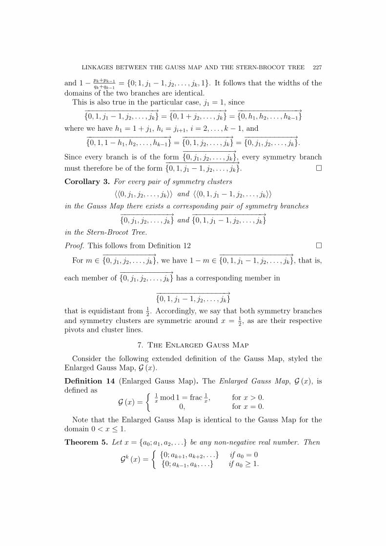
{j0; j1, . . . , jk, 1} and {j0; j1, . . . , jk}.Example 4. Consider the following clusters within G :

〈〈1〉〉 = 〈〈[1; 1] , [1; 2] , [1; 3] , . . .〉〉〈〈2〉〉 = 〈〈[2; 1] , [2; 2] , [2; 3] , . . .〉〉〈〈3〉〉 = 〈〈[3; 1] , [3; 2] , [3; 3] , . . .〉〉

...

The width of the domain of each of these clusters is equal to 1.Under K these clusters map respectively to the following branches in the

Stern-Brocot Tree:−→{1} =

{2

1,3

2,4

3, . . .

}

−→{2} =

{3

1,5

2,7

3, . . .

}

−→{3} =

{4

1,7

2,10

3

}

...

The width of the domain of each of these branches is equal to 1.

We conclude this section with some comments on G and G2.We have already seen that every part in G is mapped under K to form the

branch{

11, 1

2, 1

3, . . .

}in the left-half of the Stern-Brocot Tree. For x ≤ 1, G con-

sists of the parts [0; 1] , [0; 2] , [0; 3] , . . . which meet the x−axis at x = 1, 12, 1

3, . . .

respectively. For x > 1, G consists of only one part which is asymptotic tothe x−axis. We designate this part as [∞], the infinitieth part, because for xsufficiently large, G (x) can be made arbitrarily close to zero. Under K, [∞]maps to {∞} which is the term 1

0.

Consider G2. By Theorem 5, for x > 1, G2 (x) = frac x. Hence for x > 1, G2

is made up of disjoint truncated parts of the line y = x+1 displaced verticallydownwards by its integer parts. Though for x > 1, parts of G2 do not form acluster (parts do not become progressively more vertical), it is mapped underK to the branch

{11, 2

1, 3

1, . . .

}.


We summarise the correspondences between the Enlarged Gauss Map andthe Stern-Brocot Tree:

Summary 3. For the Enlarged Gauss Map and the Stern-Brocot Tree, underK :

1. Clusters in the Enlarged Gauss Map become branches in the Stern-BrocotTree. That is, sequential parts within a given cluster in the Enlarged GaussMap are mapped to sequential members of the corresponding branch in theStern-Brocot Tree.

2. Right branches are mapped to clusters found within even iterates; leftbranches are mapped to clusters found within odd iterates.

3. The domain of a cluster in the Enlarged Gauss Map and the domain ofits corresponding branch in the Stern-Brocot Tree are identical.

4. The cluster line x = {j0; j1, j2, . . . , jk} is associated with a cluster whichis mapped to a branch possessing the pivot {j0; j1, j2, . . . , jk}.

9. The Generalised Gauss Map

In this section we extend the domain of the Gauss Map to encompass theentire number line. We call this map the Generalised Gauss Map,G (x).

Definition 17 (Generalised Gauss Map). The Generalised Gauss Map, G (x),is defined as

G (x) =

{1x

mod 1 = frac 1x, for x 6= 0

0, for x = 0.

This definition implies that, for x 6= 0,

(9.1) G (−x) = 1−G (x) .

This is due to the fact that for negative arguments of any modulus n, we findthe difference between the next lower multiple of n and the argument itself.Since the Enlarged Gauss Map, G (x) , is the right-half of G (x) we can restateG (x) in terms of G (x). That is,

G (x) =

{ G (x) for x > 01− G (−x) for x < 0

.

A portion of the first iterate of G (x) is shown at Figure 3.But what transformation of G yields G? That is, for x > 0, 0 ≤ y ≤ 1, what

transformation converts (x, y) into (−x, 1− y) in order to create the left-halfof G? This can be achieved through two reflections: Reflect G around they− axis and then again around y = 1

2. We show that these reflections are

equivalent to (9.1).Let (x, y) be a point in R2. The transformation that reflects (x, y) around

the y−axis to give the point (−x, y) is[ −xy

]=

[ −1 00 1

] [xy

].


The transformation that reflects (x, y) around the line y = 12

to give the point(x, 1− y) is [

x1− y

]=

[01

]+

[1 00 −1

] [xy

].

We now combine these two transformations. Let (x, y) be a point in theEnlarged Gauss Map. It is transformed into the point (−x, 1− y) in the left-half of the Generalised Gauss Map according to the following transformation:[ −x

1− y

]=

[01

]+

[1 00 −1

] [ −1 00 1

] [xy

]

=

[01

]−

[xy

].

We now show that an extension of the Stern-Brocot Tree, styled the Gener-alised Stern-Brocot Tree, can be made so that it covers all rational numbers,not just the non-negative rational numbers, and that the Generalised GaussMap possesses a correspondence with the Generalised Stern-Brocot Tree.

10. The Generalised Stern-Brocot Tree

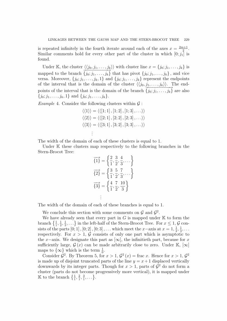
The Generalised Stern-Brocot Tree is formed from the Stern-Brocot Tree byaltering Level 0 so that it becomes:

Level 0 −10

01

10

That is, we define the Generalised Stern-Brocot Sequence by redefining H0 asH0 =

⟨−10

, 01, 1

0

⟩in Definition 7; and we define the Generalised Stern-Brocot

Tree by using H0 =⟨−1

0, 0

1, 1

0

⟩in Definition 8. Figure 1 gives the first five levels

of the Generalised Stern-Brocot Tree.Recall from (3.1) that for the Stern-Brocot Tree:

{a0; a1, a2, . . . , ak + 1} =

{Ra0+1La1Ra2 . . . Lak for k oddRa0+1La1Ra2 . . . Rak for k even.

Since the left-half of the Generalised Stern-Brocot Tree is a reflection of theStern Brocot Tree around 0

1, we have reverse movements occurring from 0

1when locating negative entries. Thus, for a0 ≥ 0, a1 ≥ 1, a2 ≥ 1, . . . , ak ≥ 1,

−{a0; a1, a2, . . . , ak + 1} =

{La0+1Ra1La2 . . . Rak for k oddLa0+1Ra1La2 . . . Lak for k even.

11. Mapping the Generalised Gauss Map to the GeneralisedStern-Brocot Tree

Since the right halves of both generalised systems are simply the EnlargedGauss Map and the Stern-Brocot Tree, for which we have previously identifiedlinkages these linkages are retained in the Generalised Gauss Map and theGeneralised Stern-Brocot Tree. However to perform mappings between the


left halves of each construction we need an expression for negative continuedfractions.

Theorem 6. For a0 ≥ 0, a1 ≥ 1, . . . , ak ≥ 1,

−{a0; a1, a2, . . . , ak} = {−a0 − 1; 1, a1 − 1, a2, . . . , ak} .

Proof.

−{a0; a1, a2, . . . , ak} = (−a0 − 1) + (1− {0; a1, a2, . . . , ak})= (−a0 − 1) + ({0; 1, a1 − 1, a2, . . . , ak}) by (6.1)

= {−a0 − 1; 1, a1 − 1, a2, . . . , ak}¤

Note that where a1 = 1, we have

{a0; a1, a2, . . . , ak} = {−a0 − 1; 1 + a2, a3, . . . , ak} .

We can now extend Definition 16 to encompass the Generalised Gauss Mapand the Generalised Stern-Brocot Tree. But firstly we define parts in Gk.

Definition 18 (Parts in the Generalised Gauss Map). [j0; j1, . . . , jk] is thatpart of Gk whose domain is [{j0; j1, . . . , jk, 1} , {j0; j1, . . . , jk}) where j0 ∈ Z,ji ∈ Z+, i > 0.

Definition 19 (Map between the Generalised Gauss Map and the GeneralisedStern-Brocot Tree). Let P be the class of all parts of all iterates of the Gen-eralised Gauss Map. Let K : P→ Q denote the map between the GeneralisedGauss Map and the Generalised Stern-Brocot Tree given by:

[j0; j1, . . . , jk]K→ {j0; j1, . . . , jk} .

That is, under K, the (j0, j1, . . . , jk)th part in Gk is transformed into the term

{j0; j1, . . . , jk} in the Generalised Stern-Brocot Tree.

Under K:1. Clusters in the Generalised Gauss Map become branches in the Gener-

alised Stern-Brocot Tree. That is, sequential parts within a given cluster aremapped to sequential members of the corresponding branch.

2. The domain of a cluster and the domain of its corresponding branch areidentical.

3. The cluster line x = {j0; j1, j2, . . . , jk} is associated with a cluster whichis mapped to a branch possessing the pivot {j0; j1, j2, . . . , jk}.


)LJXUH��/HYHOV��WR��RI�WKH�*HQHUDOLVHG�6WHUQ�%URFRW�7UHH�

� � /HYHO��

� /HYHO��

� /HYHO��

� /HYHO��

� /HYHO��

� /HYHO��


References

[1] B. Bates, M. Bunder, and K. Tognetti. Continued fractions and the Gauss map. ActaMathematica Academiae Paedagogicae Nyıregyhaziensis, 21:113–125, 2005.

[2] R. M. Corless. Continued fractions and chaos. Am. Math. Mon., 99(3):203–215, 1992.[3] R. L. Graham, D. E. Knuth, and O. Patashnik. Concrete Mathematics: a Foundation

for Computer Science. 2nd ed. Addison-Wesley Publishing Group, 1994.

Received November 2, 2005.

School of Mathematics and Applied Statistics,University of Wollongong,Wollongong, NSW, Australia 2522E-mail address: [email protected] address: [email protected] address: [email protected]

LINKAGES BETWEEN THE GAUSS MAP AND THE STERN-BROCOT TREE

Documents

Transcript of LINKAGES BETWEEN THE GAUSS MAP AND THE STERN-BROCOT TREE