1

linear programming

The linear programming deals with the optimization (maximization or

minimization ) of a function of variables known as objective function,

subject to a set of linear equation and (or) inequalities know as constraints.

The objective function may be profit , cost , production capacity or any

other measure. The restriction (constraints) may be imposed by different

sources as market demand, production process and equipment storage

capacity, etc ….

Ex: A firm produce products, these products are processed on three

different machines. The time required to manufacture one unit of each of

the three products and the daily capacity of the three machines are given in

the table below :

Time per unit ( minutes ) Machine capacity

Minutes / day Product 1 Product 2 Product 3

M1 2 3 2 440

M2 4 - 3 470

M3 2 5 - 430

It is required to determine the daily number of unites to be manufactured

for each product. The profit per unit for product 1, 2 and 3 is 4£ , 3£ and

6£ respectively.

2

Solution :

Formulation of linear programming model :-

STEP 1 From the study of the situation, we must find the key-decision to

be model. In this example, key-decision is: to decide the extent (amounts)

of products 1, 2 and 3.

STEP 2 Assume symbols for the variables of the quantities noticed in step 1.

Let the extent (amounts) of products 1, 2 and 3 manufactured daily be x1 ,

x2 and x3 respectively. Where x1 , x2 and x3 ≥ 0.

STEP 3 Mention the objective function and express it as a linear function

of variables. In the present situation, objective is to maximize the profit .

i.e. :- Z = 4x1 + 3x2 + 6x3 معادلة خطية هي دالة الهدف

STEP 4 Express the constraint as linear equalities or inequalities terms of

variables .

Here, constraints can be mathematically expressed as :-

2x1 + 3x2 + 2x3 ≤ 440 القيد االول

4x1 + 0 x2 + 3x3 ≥ 470 القيد الثاني

2x1 + 5x2 + 0x3 ≤ 430 القيد الثالث

. هذه هي الشزوط التي تىضح المسألة∴

So, the complete linear programming problem is given by :-

Maximize Z = 4x1 + 3x2 + 6x3 subject to :-

3

2x1 + 3x2 + 2x3 ≤ 440 .

4x1 + 0x2 + 3x3 ≤ 470 .

2x1 + 5x2 + 0x3 ≤ 430 .

Ex :- A company manufactures tow products A and B which the profits

per unit are 3£ and 4£ respectively. Each product is processed on tow

machines M1 and M2 . Machine M1 is available for not more than 7 hrs. 30

minutes, while machine M2 is available for 10 hrs. During any working

day, find the number of unites of products A and B to be manufactured to

get maximum profit .

Solution:-

Formulation of linear programming model :-

STEP 1 Key-decision is to determine the number of units of manufacturing

the products A and B.

STEP 2 Let these numbers of units be x1 and x2 , respectively, where x1 ,

x2 ≥ 0 .

A B

M1 1 1 450

M2 2 1 600

profit 3£ 4£

4

STEP 3 Objective function is to maximize the profit.

max Z = 3x1 + 4x2

STEP 4 Constraints are on time available to machines M1 and M2

1) 1. x1 +1. x2 ≤ 450

2) 2. x1 +1. x2 ≤ 600

So, the complete linear programming model is :-

max Z = 3x1 + 4x2

Subject to :-

1. x1 + 1. x2 ≤ 450

2. x1 + 1. x2≤ 600

Where x1 ≥ 0 , x2 ≥ 0 .

5

(( Graphical solution of two variables L.P problems ))

The L.P model which has two variable can be solved graphically. while

model with three or more variables, the graphical method is either

impractical or impossible.

Def 1 :- The area which satisfies all the constraints and the non-negativity

restriction (constraints) is called the solution space or the region of feasible

solution.

Def 2:- Any point in the solution spaces is called a feasible solution.

Def 3 :- A best feasible solution is called an optimal solution.

(( The graphical method ))

Ex :- max Z = 3x1 + 4x2

Subject to x1 + x2 ≤ 450

2x1 + x2 ≤ 600,

where x1 ≥ 0 , x2 ≥ 0.

Solution :-

1) The non-negative restrictions x1 ≥ 0 and x2 ≥ 0 imply that values of

the variables x1 and x2 can lie only in the first quadrant ( x1 , x2

plane ).

2) The inequality sign ( ≤ ) must be replaced by equality sign ( = ) for

each constraint.

6

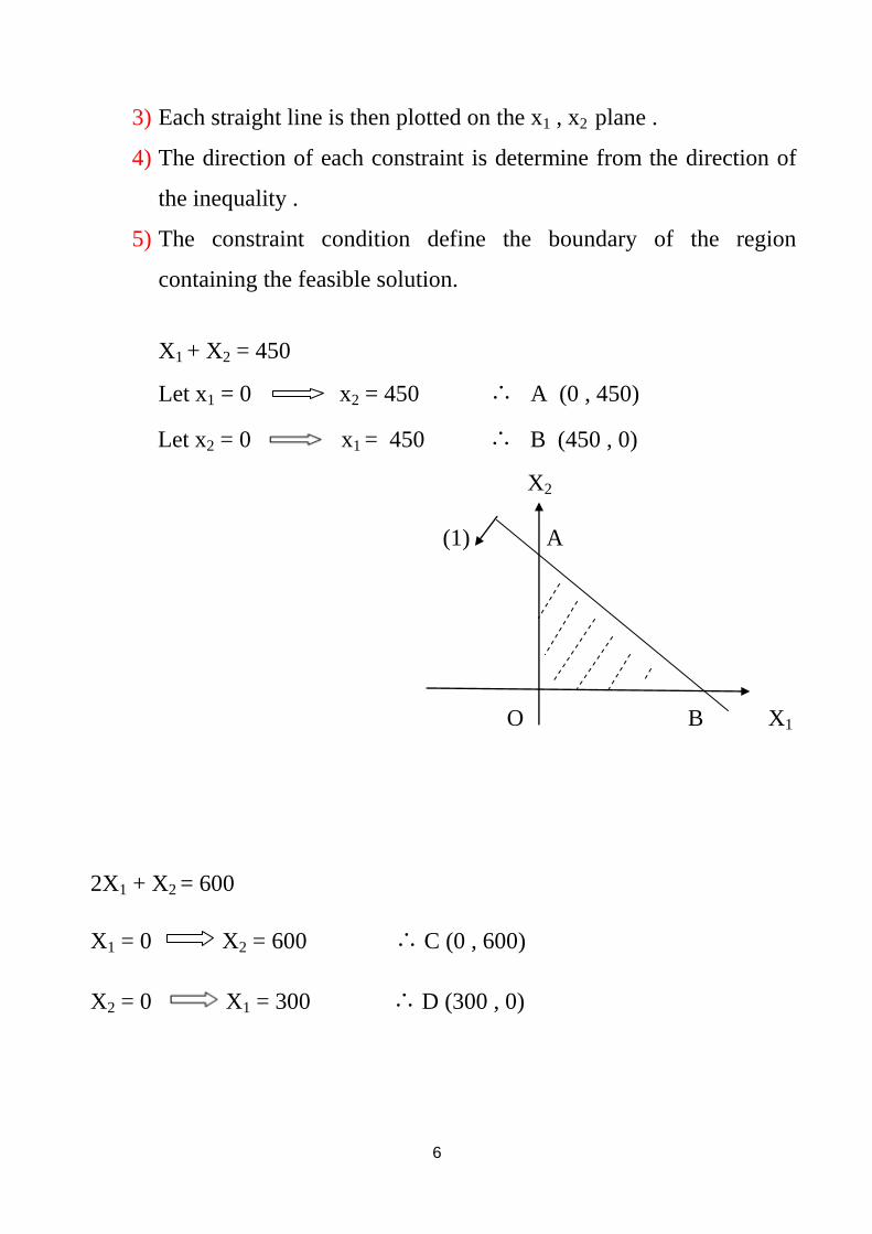
3) Each straight line is then plotted on the x1 , x2 plane .

4) The direction of each constraint is determine from the direction of

the inequality .

5) The constraint condition define the boundary of the region

containing the feasible solution.

X1 + X2 = 450

Let x1 = 0 x2 = 450 ∴ A (0 , 450)

Let x2 = 0 x1 = 450 ∴ B (450 , 0)

X2

(1) A

O B X1

2X1 + X2 = 600

X1 = 0 X2 = 600 ∴ C (0 , 600)

X2 = 0 X1 = 300 ∴ D (300 , 0)

7

X2

C

O D X1

:- اليجاد الحل االمثل و المقبىل نطابق الزسمين في رسم واحد

X2

(2)

(1) C

A E

O D B X1

The four vertices of the convex region OAED are O (0,0), A (0,450), E

(150,300), D (300,0) values the objective.

The function Z= 3x1+4x2 at these vertices are :-

Z(O) = 0, Z(A) = 1800, Z(E)= 1650, Z(D) = 900 .

Thus the maximum value of Z is 1800£ and it occurs at the vertex A

(0,450) so the solution is :-

منطقة الحل المقبىل

8

X1 = 0, X2 = 450 and max Z = 1800£ .

And this is the best solution of the problem.

Ex:- A factor produce both interior and exterior house paints. Materials A

and B are used to manufacture the point. The daily requirements of the raw

materials per ton and the availability of A and B are summarized in the

table below.

The daily demand for interior point is limited to 2 tons and cannot exceed

the exterior point by more than 1 ton.

The sale price per ton is 3000 £ and 2000 £ for the exterior and interior

paints respectively. How much interior and exterior point should the

company produce daily to maximize gross income .

Solution :- formulation of L.P. model :-

Step 1 Key decision is to determine the amount of exterior and interior

paints.

Step 2 Let these amounts are x1 and x2 respectively, where X1 ≥ 0, X2 ≥ 0.

Step 3 The objective function is to maximize the gross income. i.e. :-

Raw-materials Raw materials \ tom

Exterior Interior

Availability ton

A 1 2 6

B 2 1 8

9

Z = 3000 X1 + 2000 X2

Step 4 constraint are on availability of rows material of A and B and

the demand:-

1) 1. X1 + 2 . X2 ≤ 6

2.X1 + 1 . X2 ≤ 8

2) The demands of interior point are

X2 ≤ 2

X2 – X1 ≤ 1

Thus the L.P model is

Max Z= 3X1 + 2X2

Subject to :-

X1 + 2X2 ≤ 6

2X1 + X2 ≤ 8

X2 – X1 ≤ 1

X2 ≤ 2 X1 ≥ 0, X2 ≥ 0

1) X1 + 2X2 = 6 X1 = 0 X2 = 3 ∴ (0,3)

X2 = 0 X1= 6 ∴ (6,0)

2) 2X1 + X2 = 8 X1 = 0 X2 = 8 ∴ (0,8)

X2 = 0 X1 = 4 ∴ (4,0)

3) X2 – X1 = 1 X1 = 0 X2 = 1 ∴ (0,1)

X2 = 0 X1 = -1 ∴ (-1,0)

4) X2= 2 X1 = 0 ∴ (0,2)

10

X2

2

3

1

4

X1

X2

B C

A D

O E X1

A(0,1), E(4,0).

𝑥2 − 𝑥1 = 1 𝑥2 = 2∴ 𝑥1 = 1

𝐵 1,2 𝑥1 + 2𝑥2 = 2 𝑥2 = 2∴ 𝑥1 = 2

𝐶(2,2).

11

𝑥1 + 2𝑥2 = 62𝑥1 + 𝑥2 = 8

∴ 𝐷 = 10

3,

4

3 .

Z(A) = 2000, Z(B) = 7000, Z(C) = 10000, Z(D) = 12666,666 and

Z(E) =12000.

***************************

In the previous examples we discussed L.P. problems with optimal

solution, were it is unique. However, it may not be so for every problem.

In general a L.P problems may have :-

1) A unique optimal solution.

2) An infinite number of optimal solution.

3) Un bounded solution.

4) No solution.

Ex :- A factory used three machines M1, M2, M3 produce two parts of

product. Table below represent the machining times available on different

machines and the profit on each part

Type of machine Machine time required to reach part\minute Max. time available

per week. minute I II

M1 12 6 3000

M2 4 10 2000

M3 2 3 900

Profit 40£ 100£

12

Find the number of parts I and II to be manufacture per week to maximize

the profit.