L'INDIVIDUALITÀ DEL PARLANTE NELLE SCIENZE ...
444
L’INDIVIDUALITÀ DEL PARLANTE NELLE SCIENZE FONETICHE: APPLICAZIONI TECNOLOGICHE E FORENSI a cura di Camilla Bernardasci, Dalila Dipino, Davide Garassino, Stefano Negrinelli, Elisa Pellegrino e Stephan Schmid 8 Studi AISV SPEAKER INDIVIDUALITY IN PHONETICS AND SPEECH SCIENCES: SPEECH TECHNOLOGY AND FORENSIC APPLICATIONS ISSN: 2612-226X
-
Upload
khangminh22 -
Category
Documents
-
view
0 -
download
0
Transcript of L'INDIVIDUALITÀ DEL PARLANTE NELLE SCIENZE ...

L’INDIVIDUALITÀ DEL PARLANTENELLE SCIENZE FONETICHE:APPLICAZIONI TECNOLOGICHEE FORENSI
a cura diCamilla Bernardasci, Dalila Dipino,Davide Garassino, Stefano Negrinelli,Elisa Pellegrino e Stephan Schmid
8Studi AISV
SPEAKER INDIVIDUALITY IN PHONETICSAND SPEECH SCIENCES: SPEECH TECHNOLOGY AND FORENSIC APPLICATIONS
ISSN: 2612-226X

L’INDIVIDUALITÀ DEL PARLANTE NELLE SCIENZE FONETICHE: APPLICAZIONI TECNOLOGICHE E FORENSI
SPEAKER INDIVIDUALITY IN PHONETICS AND SPEECH SCIENCES: SPEECH TECHNOLOGY AND FORENSIC APPLICATIONS
a cura di Camilla Bernardasci, Dalila Dipino, Davide Garassino, Stefano Negrinelli, Elisa Pellegrino e Stephan Schmid
Milano 2021

© 2021 AISV - Associazione Italiana Scienze della Voce c/o LUSI Lab - Dip. di Scienze Fisiche Complesso Universitario di Monte S. Angelo via Cynthia snc 80135 Napoli email: [email protected] sito: www.aisv.it
Edizione realizzata da Officinaventuno Via F.lli Bazzaro, 18 20128 Milano - Italy email: [email protected] sito: www.officinaventuno.com ISBN edizione digitale: 978-88-97657-54-5 ISSN: 2612-226X
studi AISV - Collana peer reviewed
Studi AISV è una collana di volumi collettanei e monografie dedicati alla dimensio-ne sonora del linguaggio e alle diverse interfacce con le altre componenti della gram-matica e col discorso. La collana, programmaticamente interdisciplinare, è aperta a molteplici punti di vista e argomenti sul linguaggio: dall’attenzione per la struttura sonora alla variazione sociofonetica e al mutamento storico, dai disturbi della parola alle basi cognitive e neurobiologiche delle rappresentazioni fonologiche, fino alle applicazioni tecnologiche.
I testi sono sottoposti a processi di revisione anonima fra pari che ne assicurano la conformità ai più alti livelli qualitativi del settore.
I volumi sono pubblicati nel sito dell’Associazione Italiana di Scienze della Voce con accesso libero a tutti gli interessati.
Curatore/EditorCinzia Avesani (CNR-ISTC)
Curatori Associati/Associate EditorsFranco Cutugno (Università di Napoli), Barbara Gili Fivela (Università di Lecce), Daniel Recasens (Università di Barcellona), Antonio Romano (Università di Torino), Mario Vayra (Università di Bologna).
Comitato Scientifico/Scientific CommitteeGiuliano Bocci (Università di Siena), Silvia Calamai (Università di Siena), Mariapaola D’Imperio (Rutgers University), Giovanna Marotta (Università di Pisa), Stephan Schmid (Università di Zurigo), Carlo Semenza (Università di Padova), Alessandro Vietti (Libera Università di Bolzano), Claudio Zmarich (CNR-ISTC).

Sommario
CAMILLA BERNARDASCI, DALILA DIPINO, DAVIDE GARASSINO, STEFANO NEGRINELLI, ELISA PELLEGRINO, STEPHAN SCHMID
Prefazione 7
PARTE I Individualità del parlante, riconoscimento della voce e fonetica forense
HELEN FRASER
Forensic Transcription: Legal and scientific perspectives 19
KIRSTY MCDOUGALL
Ear-catching versus eye-catching? Some developments and current challenges in earwitness identification evidence 33
KATHARINA KLUG, MICHAEL JESSEN, YOSEF A. SOLEWICZ, ISOLDE WAGNER
Collection and analysis of multi-condition audio recordings for forensic automatic speaker recognition 57
JUSTIN J.H. LO
Seeing the trees in the forest: Diagnosing individual performance with acoustic data in likelihood ratio based forensic voice comparison 77
BENJAMIN O’BRIEN, CHRISTINE MEUNIER, ALAIN GHIO, CORINNE FREDOUILLE, JEAN-FRANÇOIS BONASTRE, CAROLANNE GUARINO
Discriminating speakers using perceptual clustering interface 97
THAYABARAN KATHIRESAN
Gender bias in voice recognition: An i- and x-vector-based gender-specific automatic speaker recognition study 113
MARCO FARINELLA, MARCO CARNAROGLIO, FABIO CIAN
Una nuova idea di “impronta vocale” come strumento identificativo e riabilitativo 123
ALICE ALBANESI, SONIA CENCESCHI, CHIARA MELUZZI, ALESSANDRO TRIVILINI
Italian monozygotic twins’ speech: a preliminary forensic investigation 135
4 SOMMARIO
CAROLINA LINS MACHADO
A cross-linguistic study of between-speaker variability in intensity dynamics in L1 and L2 spontaneous speech 157
ANGELIKA BRAUN
The notion of speaker individuality and the reporting of conclusions in forensic voice comparison 175
PARTE II Prosodia, sociofonetica e coarticolazione
SALVATORE GIANNINÒ, CINZIA AVESANI, GIULIANO BOCCI, MARIO VAYRA
Giudice o imputato? La prosodia implicita e la risoluzione di ambiguità sintattiche globali 195
DAVIDE GARASSINO, DALILA DIPINO, FRANCESCO CANGEMI
Per un approccio multidimensionale allo studio dell’intonazione: le domande in genovese 219
LOREDANA SCHETTINO, SIMON BETZ, FRANCESCO CUTUGNO, PETRA WAGNER
Hesitations and individual variability in Italian tourist guides’ speech 243
GLENDA GURRADO
Sulla codifica e decodifica della sorpresa 263
VALENTINA DE IACOVO, MARCO PALENA, ANTONIO ROMANO
Evaluating prosodic cues in Italian: the use of a Telegram chatbot as a CALL tool for Italian L2 learners 283
DUCCIO PICCARDI, FABIO ARDOLINO
Gaming variables in linguistic research. Italian scale validation and a Minecraft pilot study 299
ELISA PELLEGRINO
Dynamics of short-term cross-dialectal accommodation. A study on Grison and Zurich German 325
MANUELA FRONTERA
Radici identitarie e mantenimento linguistico: il caso di un gruppo di heritage speakers di origine calabrese 343
SONIA D’APOLITO, BARBARA GILI FIVELA
Interazione tra accuratezza, contesto e co-testo in Italiano L2: le affricate prodotte da francofoni 371

SOMMARIO 5
CECILIA VALENTINI, SILVIA CALAMAI
Sull’insegnamento della pronuncia italiana negli anni sessanta a bambini e a stranieri 391
CHIARA BERTINI, PAOLA NICOLI, NICCOLÒ ALBERTINI, CHIARA CELATA
A 3D model of linguopalatal contact for virtual reality biofeedback 403
CLAUDIO ZMARICH, ANNAROSA BIONDI, SERENA BONIFACIO, MARIA GRAZIA BUSÀ, BENEDETTA COLAVOLPE, MARIAVITTORIA GAIOTTO, FRANCESCO OLIVUCCI
Coarticulation and VOT in an Italian child from 18 to 48 months of age 413
Autori 437


CAMILLA BERNARDASCI, DALILA DIPINO, DAVIDE GARASSINO, STEFANO NEGRINELLI, ELISA PELLEGRINO, STEPHAN SCHMID
Prefazione
Il presente volume, che raccoglie una selezione di contributi presentati al XVII Convegno Nazionale dell’Associazione Italiana di Scienze delle Voce (AISV), ha come oggetto l’individualità del parlante e le sue possibili applicazioni tecnologi-che e forensi, tema di crescente attualità nell’ambito delle scienze fonetiche. Com’è noto, le scienze del linguaggio tendono a privilegiare prospettive di ricerca incentra-te sull’analisi del sistema linguistico o sulla variazione determinata da fattori socio-linguistici, quali la provenienza geografica e sociale del parlante oppure il contesto situazionale. Le scienze della voce, invece, hanno come oggetto di studio anche gli aspetti materiali della produzione e della percezione dei messaggi verbali. Per questo motivo la variazione a livello individuale – lungi dall’essere una fonte di ‘disturbo’ o di ‘rumore’ – diviene essa stessa un fenomeno di interesse. Le dimensioni di va-riazione legate al parlante acquisiscono, inoltre, una rilevanza centrale per la ricerca applicata nel campo delle tecnologie del parlato (si pensi ad esempio al riconosci-mento automatico del linguaggio e del parlante) e, in particolare, nell’ambito della fonetica forense.
Il convegno, inizialmente concepito per svolgersi in presenza all’Università di Zurigo, a causa delle restrizioni dovute alla pandemia di coronavirus, si è tenuto onli-ne nelle giornate del 4 e 5 febbraio 2021, raggiungendo picchi di partecipazione superiori ai 150 convegnisti. Le due giornate sono state aperte dalle sedute plenarie di Helen Fraser (University of New England) e Kirsty McDougall (University of Cambridge) su temi di fonetica forense, a cui sono dedicati i primi due contributi del presente volume. La fonetica forense è stata oggetto anche della tavola rotonda intitolata “Current trends and issues in forensic phonetics research”, che si è svolta in chiusura del convegno e alla quale hanno partecipato – moderati da Peter French – i seguenti relatori (in ordine alfabetico): Volker Dellwo (Universität Zürich), Mirko Grimaldi (Università del Salento), Michael Jessen (Bundeskriminalamt, Wiesbaden) e Kirsty McDougall (University of Cambridge). Il convegno è stato preceduto da un workshop, diretto da Michael Jessen, sui metodi di riconoscimento automatico e se-miautomatico del parlante. Tuttavia, a rappresentare la maggior parte dei lavori sono state le 22 relazioni orali e le 24 presentazioni di poster che si sono succedute nei due giorni del convegno. Seguendo la tradizione dei convegni AISV, accanto a contributi dedicati al tema specifico di questa edizione, sono state accolte anche proposte di comunicazione ‘a tema libero’, dedicate ai molteplici aspetti della ricerca in fonetica.
Come di consueto, con l’inoltro della versione scritta del proprio contributo, giovani autori, studenti, dottorandi e ricercatori non strutturati hanno avuto la pos-

8 C. BERNARDASCI, D. DIPINO, D. GARASSINO, S. NEGRINELLI, E. PELLEGRINO, S. SCHMID
sibilità di concorrere per il Premio Franco Ferrero, istituito nel 2006. La vincitrice del premio per la sezione ‘Linguistica, Fonetica, Fonologia’ è stata Manuela Frontera, autrice dello studio sociolinguistico Radici identitarie e mantenimento linguistico: il caso di un gruppo di heritage speakers di origine calabrese. Nella sezione ‘Tecnologie del parlato’ il premio è invece stato vinto da Justin H. Lo per il suo contributo Seeing the trees in the forest: Diagnosing individual performance with acoustic data in likeliho-od ratio based forensic voice comparison.
Il volume è articolato in due parti. La prima parte, intitolata Individualità del parlante, riconoscimento della voce e fonetica forense / Speaker individuality, Voice re-cognition, and Forensic phonetics, raccoglie dieci contributi dedicati all’individua-lità del parlante o alla fonetica forense in generale. Nella seconda parte, intitolata Prosodia, sociofonetica e coarticolazione / Prosody, Sociophonetics, and Coarticulation, seguono dodici contributi che trattano vari aspetti della ricerca fonetica.
La pubblicazione si apre con il contributo di Helen Fraser che, basandosi sulla sua decennale esperienza come consulente linguistica per i tribunali australiani, af-fronta una questione di notevole rilevanza giuridica, ovvero la trascrizione di regi-strazioni audio in ambito forense. In base all’analisi di tracce audio (disponibili sul sito web dell’autrice), si evidenziano i problemi connessi all’utilizzo di trascrizioni elaborate da poliziotti, come ad esempio il priming contestuale. Si discute inoltre il caso dell’Australia dove, a seguito di una lettera firmata da quattro associazioni di linguistica, è stato istituito il Research Hub for Language in Forensic Evidence, presso l’Università di Melbourne. L’autrice sostiene che la trascrizione in ambito forense rappresenti un tipo particolare di investigazione fonetica che deve tener conto, al di là dell’evidenza bottom-up fornita dall’analisi acustica, anche di processi top-down determinati da vari fattori contestuali.
Il contributo di Kirsty McDougall si occupa di un altro aspetto estremamente rilevante nella prassi forense, ovvero l’identificazione di voci tramite testimonianze uditive. Nei casi in cui non sono disponibili registrazioni sonore degli imputati si ricorre talvolta alla tecnica di identificazione nota come Voice Parade, in cui un cer-to numero di ascoltatori è chiamato a valutare, ad esempio, la somiglianza tra una serie di voci. Basandosi sulla prassi vigente in Inghilterra e nel Galles, l’autrice offre una rassegna degli sviluppi più recenti in quest’ambito, descrivendo nel dettaglio i vari tipi di esperimenti percettivi adottati e discutendo le somiglianze e le differenze tra il processo di riconoscimento del parlante su base visiva e quello su base uditi-va. Nello specifico, si presentano i risultati di due studi condotti all’Università di Cambridge, basati su apposite banche dati di voci, oggetto di valutazione percettiva da parte di un numero di ascoltatori piuttosto elevato. Il primo studio confronta sul piano percettivo e acustico la somiglianza tra voci aventi lo stesso accento regiona-le o accenti regionali diversi, considerando parametri acustici come l’analisi delle formanti a lungo termine e la velocità di articolazione. Il secondo studio analizza l’effetto della durata degli stimoli sull’accuratezza del riconoscimento delle voci, ravvisando nella soglia tra i 15 e i 30 secondi la durata sufficiente a garantirne una valutazione affidabile.

PREFAZIONE 9
Nel lavoro di Katharina Klug, Michael Jessen, Yosef A. Solewicz e Isolde Wagner viene introdotto FORBIS, un progetto volto alla raccolta di un corpus di registrazioni utilizzate in indagini forensi, impiegabili per validare sistemi di riconoscimento automatico del parlante con materiali analoghi a quelli adottati nei casi giudiziari. Nel contributo vengono delineate le problematicità insite nella raccolta di un tal tipo di corpus e si presentano i risultati dei primi test di vali-dazione effettuati sul sistema VOCALISE (VOice Comparison and Analysis of the LIkelihood of Speech Evidence – v. 2.7), con voci di parlanti tedescofoni, in condizioni di registrazione equivalenti (messaggi vocali – messaggi vocali) o dif-ferenti (messaggi vocali – telefonate). Si discutono le variazioni delle prestazioni del sistema VOCALISE, quantificate tramite le metriche Equal Error Rate e Log-Likelihood-Ratio Cost, per effetto delle procedure di normalizzazione e calibrazio-ne, e si analizzano le distribuzioni dei punteggi relativi alle comparazioni tra gli stessi parlanti e parlanti diversi, mediante i Tippet plots.
Il contributo di Justin H. Lo parte dall’assunto che la ricerca in fonetica forense ha finora trascurato la variazione individuale e i fattori a essa soggiacenti. Prendendo in esame la distribuzione globale dei valori formantici in un corpus di francese e inglese del Canada, l’autore propone una classificazione dei parlanti sulla base del modello biometrico di Doddington e colleghi. Secondo tale modello, il comporta-mento acustico di ciascun parlante viene associato ad un diverso animale, a seconda del grado con cui viene correttamente identificato con altri parlanti in una proce-dura di riconoscimento automatico. Un’analisi acustica rivela poi come due gruppi di parlanti tra loro distinti, classificati come ‘colombe’ e ‘vermi’, i due poli estremi della scala di riconoscibilità secondo il modello biometrico, presentano al loro inter-no distribuzioni dei valori formantici molto simili. In conclusione, classificazione biometrica e analisi acustica mostrano l’importanza di un’indagine che prenda le mosse dal livello individuale.
Nel lavoro di Benjamin O’Brien, Christine Meunier, Alain Ghio, Corinne Fredouille, Jean-François Bonastre e Carolanne Guarino viene proposto un metodo alternativo ai tradizionali test di identificazione e discriminazione dei parlanti, basa-to sul clustering percettivo. L’obiettivo degli autori è duplice: da un lato valutare l’ef-ficacia della nuova metodica su ascoltatori non esperti; dall’altro verificare la con-gruenza tra le performance di questi ultimi e quella di un sistema di riconoscimento automatico del parlante, precedentemente utilizzato per la selezione degli stimoli oggetto del test. I partecipanti allo studio avevano il compito di raggruppare gli stimoli in cinque gruppi, ciascuno rappresentativo di un parlante diverso. La perfor-mance degli ascoltatori è stata esaminata su due diverse batterie di stimoli mediante il Coefficiente di Correlazione di Mathews e una metrica ideata per valutare la pu-rezza dei cluster ottenuti. I risultati hanno evidenziato spiccate capacità discrimina-torie nei soggetti sottoposti al test di clustering, provando al contempo la validità del test, e una significativa correlazione tra gli esiti del clustering percettivo e le distanze acustiche tra i parlanti calcolate dal sistema di riconoscimento automatico.

10 C. BERNARDASCI, D. DIPINO, D. GARASSINO, S. NEGRINELLI, E. PELLEGRINO, S. SCHMID
Il contributo di Thayabaran Kathiresan si sofferma principalmente sull’impatto esercitato dalle voci femminili, a confronto con quelle maschili, sulle prestazioni di sistemi di riconoscimento automatico del parlante di tipo i-vector e x-vector. L’autore utilizza un dataset di voci di parlanti inglesi e di cinese mandarino, bilanciato per genere, estratto da quattro corpora multilingui: Voxceleb1 e 2 sono stati impiegati per l’addestramento dei modelli di riconoscimento; TIMIT e AISHELL-1, invece, per la verifica delle prestazioni del sistema. I modelli di riconoscimento sono stati addestrati mediante voci dello stesso genere e di generi diversi; le prestazioni del si-stema, invece, sono state valutate esclusivamente mediante dataset di voci omogenee per genere. I risultati delle analisi hanno evidenziato per le voci femminili, rispetto a quelle maschili, un peggioramento nelle prestazioni del sistema in termini di Equal Error Rate, indipendentemente dalla lingua dei parlanti e dal tipo di sistema im-piegato (i-vector o x-vector). Dei due, come atteso, l’accuratezza del sistema di tipo x-vector è risultata superiore a quella del sistema di tipo i-vector.
Marco Farinella, Marco Carnaroglio e Fabio Cian propongono una nuova defi-nizione del concetto di ‘impronta vocale’, già impiegata con successo nel campo del-la riabilitazione, che potrebbe trovare future applicazioni in ambito forense. Sulla base di un campione di più di mille soggetti, il contributo esplora la correlazione tra l’intero spettro di frequenze emesse dalla voce umana e le caratteristiche fisiologiche di chi l’ha prodotta, al fine di individuare la cosiddetta ‘impronta vocale’, ovvero una configurazione frequenziale in grado di identificare le peculiarità fisiche ed emotive di un soggetto. Ciò è reso possibile grazie al confronto dello spettro sonoro delle voci con un modello ideale preso come riferimento. Tale modello si è rivelato par-ticolarmente utile in prospettiva riabilitativa, come stimolo per il miglioramento della prestazione fonatoria. Grazie al suo utilizzo, infatti, in un secondo test che ha coinvolto 171 soggetti, l’affaticamento glottico dei partecipanti si è notevolmente ridotto e la percezione del loro stato psicofisico ed emotivo è migliorata.
Il contributo di Alice Albanesi, Sonia Cenceschi, Chiara Meluzzi e Alessandro Trivillini studia la possibilità di distinguere un parlante dal suo gemello in registra-zioni sonore di bassa qualità. In questo studio preliminare è stata condotta un’ana-lisi su dati qualitativi e quantitativi per confrontare il parlato di quattro coppie di gemelli omozigoti italofoni (due di maschi e due di femmine). Le distribuzioni del-la frequenza fondamentale e delle formanti sono risultate simili tra le diverse cop-pie di gemelli, anche se una differenza è osservabile grazie alla normalizzazione di Lobanov, e ciò soprattutto in contesto di parlato controllato. L’analisi statistica ha confermato questi risultati e ha evidenziato alcune differenze nei valori formantici e il ruolo della F3. I risultati, discussi in una prospettiva forense, potranno essere inte-grati grazie a ulteriori esperimenti, così da accrescere il campione di dati e la serie di caratteristiche osservate, con lo scopo di determinare la validità della metodologia qui presentata per la discriminazione dei gemelli mediante evidenze acustiche.
Nel suo contributo, Carolina Lins Machado esamina la variabilità intra- e in-ter-linguistica nelle dinamiche di intensità, intese come l’andamento dell’energia acustica associata al gesto articolatorio di apertura (dinamica positiva) e chiusura

PREFAZIONE 11
(dinamica negativa) della bocca nella transizione tra vocale e consonante. In parti-colare, il lavoro si propone di analizzare le dinamiche di intensità nel parlato sponta-neo di parlanti olandesi bilingui, nella loro lingua madre (L1) e in inglese. I risultati sembrano suggerire che le dinamiche di intensità costituiscano un buon indicatore della variabilità tra parlanti, al di là della lingua in uso, avvalorando la tesi che le dif-ferenze nella realizzazione dell’intensità siano da attribuire anche a caratteristiche biomeccaniche individuali. Sembra inoltre che le dinamiche di intensità negative si-ano più variabili rispetto a quelle positive, poiché probabilmente il parlante esercita un controllo minore sul gesto di chiusura che su quello di apertura. Ciò vale in par-ticolare per la L1 rispetto alla seconda lingua (L2), in cui prevale invece la tendenza ad un gesto articolatorio più accurato.
Il lavoro di Angelika Braun offre un punto di vista critico su alcuni strumenti co-munemente utilizzati per la comparazione vocale nella pratica forense. In particola-re, l’autrice sostiene che i risultati ottenuti tramite la metrica Likelihood ratio non si-ano in realtà così obiettivi e inequivocabili come sarebbe lecito aspettarsi. L’articolo discute poi i risultati di un sondaggio rivolto a giudici e pubblici ministeri tedeschi, in cui si chiedeva loro di valutare le conclusioni di un esame di comparazione vocale. Queste ultime erano state formulate in due modi diversi, il primo basato sulle scale verbali di probabilità, notoriamente considerate poco affidabili dal punto di vista logico e statistico, il secondo sulla metrica Likelihood ratio, un metodo ritenuto più preciso e obiettivo. I risultati dell’inchiesta mostrano molto chiaramente come le conclusioni basate su scale verbali ottengano da parte dei partecipanti all’esperi-mento valutazioni significativamente più alte rispetto a quelle basate sulla metrica Likelihood ratio.
La seconda parte del volume si apre con il contributo di Salvatore Gianninò, Cinzia Avesani, Giuliano Bocci e Mario Vayra che affrontano la problematica della risoluzione di ambiguità sintattiche globali. In frasi come ‘Ha dimostrato la falsità delle accuse al comandante’, infatti, l’ultimo sintagma preposizionale (SP) può es-sere o un complemento del verbo ‘ha dimostrato’ o un complemento del sintagma nominale (SN) ‘accuse’: le due interpretazioni sono ugualmente possibili. Tuttavia, lingue diverse mostrano preferenze distinte per l’una o per l’altra interpretazione. Poiché la scansione prosodica può disambiguare la struttura sintattica, la Implicit Prosody Hypothesis postula che, anche durante la lettura silenziosa, una struttura prosodica disambiguante sia proiettata sullo stimolo visivo. Le differenze inter-linguistiche nella preferenza di una delle due risoluzioni sarebbero motivate dalla varietà dei sistemi prosodici. Per verificare questa ipotesi, gli autori del contributo hanno condotto uno studio su venti parlanti italiani, dal quale emerge, tra gli altri aspetti, che la lettura all’impronta di frasi con ambiguità sintattiche globali è in-fluenzata dalla lunghezza dei costituenti.
L’articolo di Davide Garassino, Dalila Dipino e Francesco Cangemi offre uno studio intonativo delle frasi interrogative in genovese, esplorandone la variazione per mezzo di un approccio ‘multidimensionale’, che, oltre agli aspetti prosodici, tie-ne in considerazione anche quelli pragmatici e interazionali. Il lavoro presenta inol-

12 C. BERNARDASCI, D. DIPINO, D. GARASSINO, S. NEGRINELLI, E. PELLEGRINO, S. SCHMID
tre la prima applicazione del periogramma allo studio di una varietà linguistica non standard. Questa tecnica di visualizzazione di F0 si basa sulla misurazione dell’ener-gia periodica e, grazie alla sua accuratezza fonetica, si mostra particolarmente adatta all’esame di dati raccolti tramite un’indagine sul campo. L’analisi intonativa con-ferma la presenza di una notevole variazione prosodica delle domande polari, che rispecchia la situazione già osservata da alcuni studi relativi all’italiano regionale di Genova, così come l’associazione tra specifici profili melodici e particolari forme (domande polari vs parziali) e funzioni (domande retoriche).
Lo studio di Loredana Schettino, Simon Betz, Francesco Cutugno e Petra Wagner riguarda le strategie di esitazione che le guide turistiche possono adottare per gestire il proprio discorso, con particolare attenzione alla variabilità individua-le. Lavori precedenti hanno sottolineato che i fenomeni di esitazione possono co-stituire uno strumento utile per strutturare il discorso e catturare l’attenzione dei visitatori, e che il comportamento linguistico idiosincratico può influenzare la loro produzione. Alla luce di questi risultati, nel contributo si analizzano aspetti formali, fonetici e funzionali delle esitazioni all’interno di un piccolo corpus costituito da discorsi di guide turistiche italiane. Lo scopo è quello di descrivere gli usi individuali e generali delle esitazioni e di stabilire se i diversi tipi di esitazione e le loro caratte-ristiche fonetiche correlino con determinate funzioni discorsive.
Il lavoro di Glenda Gurrado è dedicato alla ricerca su un’emozione poco indaga-ta negli studi del settore: la sorpresa, che può assumere una connotazione positiva o negativa. Il contributo mira a definirne i correlati acustici, sia in produzione sia in percezione, e a verificare eventuali differenze a livello prosodico nel caso di sorpresa positiva o negativa. L’analisi acustica di un campione di 20 frasi esclamative pronun-ciate da informatori baresi mostra che la sorpresa presenta un’estensione tonale più ampia, valori di F0 più alti, un’intensità media e una durata maggiori rispetto agli enunciati neutrali. Inoltre, la sorpresa positiva pare più marcata a livello prosodico rispetto alla sorpresa negativa. Dal punto di vista percettivo, tuttavia, la manipo-lazione di alcuni parametri prosodici, quali F0 e durata, non sembra condizionare significativamente il grado di sorpresa percepito dagli uditori.
Il lavoro di Valentina De Iacovo, Marco Palena e Antonio Romano descrive l’uso didattico di un chatbot per la piattaforma di messaggistica istantanea Telegram, il cui scopo è offrire agli apprendenti di italiano come lingua seconda una valutazione au-tomatica del proprio livello di accuratezza intonativa, verificata tramite il confronto con parlanti nativi. Dalle produzioni dei parlanti nativi e degli apprendenti ottenute tramite il chatbot, gli autori hanno estratto alcuni parametri ritmico-prosodici, quali il numero di sillabe, la durata delle pause e il numero di segmenti di ogni enunciato. I risultati dell’analisi suggeriscono l’utilità di integrare questi indici acustici fra i cri-teri di valutazione del chatbot, alla luce delle notevoli differenze mostrate da parlanti nativi e apprendenti. Infine, gli autori propongono altre migliorie al software, tra le quali una maggior varietà di funzioni comunicative e atti linguistici.
Il contributo di Duccio Piccardi e Fabio Ardolino affronta il tema della ludiciz-zazione dei protocolli d’inchiesta linguistica. Gli autori esaminano gli effetti del-

PREFAZIONE 13
le variabili User Engagement (coinvolgimento nell’esperienza di gioco) e Gaming Literacy (familiarità con l’attività proposta) in un esperimento pilota sulla realiz-zazione della gorgia a Firenze. L’esperimento adotta un protocollo di raccolta ludi-cizzato, in cui ogni soggetto prende parte ad una sessione del videogioco Minecraft: Education Edition insieme allo sperimentatore. Lo studio persegue un duplice obiet-tivo: da un lato, si propone di valutare alcune scale di misura usate nei protocolli lu-dicizzati, adattando all’italiano strumenti di valutazione già esistenti; dall’altro, su un piano più dialettologico, intende studiare le varianti non spiranti delle occlusive sorde (laddove in posizione postvocalica, per il fenomeno della gorgia fiorentina, ci aspetteremmo varianti fricative). I risultati mostrano che entrambe le variabili esa-minate, ossia User Engagement e Gaming Literacy, hanno un effetto positivo sull’uso di varianti occlusive, sebbene per meccanismi diversi.
Il contributo di Elisa Pellegrino si focalizza sul tema dell’adattamento fonetico in contesti di contatto interdialettale. L’autrice si propone di indagare se fenomeni di convergenza documentati sul piano vocalico si osservino nelle stesse coppie di parlanti anche sul piano ritmico. Il corpus esaminato consiste in entrate lessicali prodotte da singoli locutori zurighesi e grigionesi immediatamente prima e dopo aver partecipato a due compiti di parlato semi-spontaneo. Di ciascuna entrata les-sicale sono state misurate le durate delle sonoranti intervocaliche, delle vocali in sillaba aperta e in fine di parola, e successivamente calcolate le distanze acustiche tra i membri di ciascuna coppia nelle produzioni pre- e post-dialogiche. L’analisi dell’a-dattamento ritmico, misurato mediante il computo della ‘differenza nelle distanze tra i singoli parlanti di una coppia’ non ha rilevato variazioni significative nella re-alizzazione delle tre caratteristiche temporali, evidenziando così un’asimmetria nei locutori zurighesi e grigionesi tra l’adattamento vocalico e quello ritmico.
Lo studio sociofonetico di Manuela Frontera analizza gli effetti di vari fattori psicosociali sull’aspirazione di /p t k/ in posizione post-sonorante nel dialetto di dieci emigrati calabresi residenti da molti decenni in Argentina. In base a interviste sociolinguistiche con i parlanti sono stati rilevati quattro ‘indicatori psicosociali’: nello specifico, la frequenza d’uso di varietà in contatto, gli atteggiamenti verso le varietà ereditarie, il livello di integrazione nella società argentina e il legame con il dialetto e la Calabria. Il rapporto tra questi fattori psicosociali e la variabile acustica del Voice Onset Time (VOT) è stato analizzato attraverso vari modelli statistici (tra cui l’analisi delle componenti principali e modelli a effetti misti). Da queste anali-si risulta, ad esempio, che il mantenimento del tratto di aspirazione è influenzato maggiormente dagli atteggiamenti linguistici che non dalla frequenza d’uso delle varietà ereditarie.
Il contributo di Sonia D’Apolito e Barbara Gili Fivela si concentra sull’influenza della L1, del contesto e del co-testo sull’accuratezza nella pronuncia di suoni non nativi. Lo studio si basa su realizzazioni di affricate italiane prodotte da studen-ti francesi di italiano L2 (principianti e avanzati). Lo scopo è quello di verificare l’accuratezza della produzione di questi suoni non nativi in diversi compiti (con-testi globali) e variando la quantità di informazioni disponibili nel testo (co-testo).

14 C. BERNARDASCI, D. DIPINO, D. GARASSINO, S. NEGRINELLI, E. PELLEGRINO, S. SCHMID
I parametri acustici analizzati quali indici dell’accuratezza nella produzione delle affricate sono la durata delle consonanti affricate e delle vocali seguenti nonché la velocità di eloquio. I risultati mostrano che, soprattutto negli studenti avanzati, il co-testo influenza l’accuratezza nella produzione delle affricate più del contesto.
Il lavoro di Cecilia Valentini e Silvia Calamai analizza, nel quadro della storia della pronuncia italiana, due corsi di ortoepia risalenti agli anni Sessanta, uno pensa-to per i bambini e uno dedicato agli studenti stranieri di italiano. Nel tempo la pro-nuncia della lingua italiana è stata molto discussa dagli esperti: la pronuncia stan-dard, basata sull’inflessione fiorentina che si trova nei libri di testo e nei dizionari, è il risultato di una norma altamente fittizia che non è stata adottata dalle comunità di lingua italiana. L’esame dei due corsi di ortoepia mostra infatti come la dizione standard non sia stata utilizzata nemmeno nelle pubblicazioni istituzionali. Nello studio, inoltre, si illustra come la pronuncia presentata nei due corsi sia fortemente influenzata dall’ortografia e dai fenomeni fonetici che si sarebbero ampiamente dif-fusi nei decenni successivi.
Modellare la dinamica spazio-temporale del contatto linguopalatale risulta par-ticolarmente importante nel contesto delle patologie del linguaggio sia per la dia-gnosi che per la riabilitazione. L’articolo di Chiara Bertini, Paola Nicoli, Niccolò Albertini e Chiara Celata descrive un modello tridimensionale del contatto linguo-palatale, ricavato da dati fonetici reali multilivello prodotti da un parlante italiano. Il modello permette la simulazione in un ambiente di realtà virtuale dei meccanismi alla base della produzione di consonanti e vocali linguali. Gli autori descrivono inol-tre le procedure che hanno permesso lo sviluppo del modello e del suo risultato, vale a dire un’applicazione animata, fruibile all’interno di un motore grafico Unity 3D, utilizzabile sia in modalità desktop sia in ambiente immersivo.
Lo studio di Claudio Zmarich, Annarosa Biondi, Serena Bonifacio, Maria Grazia Busà, Benedetta Colavolpe, Mariavittoria Gaiotto e Francesco Olivucci ha l’obiet-tivo di apportare nuovi dati per lo studio di due aspetti poco trattati nello sviluppo del linguaggio infantile in ambito italofono: il VOT e la coarticolazione anticipata C-V. A tale scopo, una bambina originaria di Trieste è stata registrata con cadenza trimestrale, dai 18 a 48 mesi d’età. La giovane informatrice ha interagito con il per-sonale medico in contesto ludico, ripetendo più volte ogni pseudo-parola bisillabica iniziante per consonante occlusiva sorda o sonora, seguita dalle vocali /a/ e /i/. I risultati emersi si possono riassumere nel seguente modo: 1) VOT: le occlusive so-nore risultano più difficili da produrre rispetto a quelle sorde, e il contrasto sordo vs sonoro appare acquisito solo a partire dai 30 mesi di età; 2) Coarticolazione: il grado di coarticolazione aumenta con l’età, ma a 48 mesi le occlusive bilabiali e alveolari sono ancora meno coarticolate che in soggetti adulti. Il grado di coarticolazione era legato alla competizione fra gli organi articolatori nel realizzare gesti adiacenti.
I curatori del presente volume ringraziano sentitamente tutti i membri del Comitato Scientifico del XVII Convegno AISV e tutti gli studiosi che hanno valu-tato le proposte di comunicazione per il convegno, fungendo successivamente anche da revisori dei contributi scritti: Cinzia Avesani (ISTC-CNR, Padova), Pier Marco

PREFAZIONE 15
Bertinetto (Scuola Normale Superiore, Pisa), Silvia Calamai (Università di Siena), Francesco Cangemi (Universität zu Köln), Chiara Celata (Università degli Studi di Urbino Carlo Bo), Sonia Cenceschi (Scuola Universitaria Professionale della Svizzera Italiana, SUPSI), Francesco Cutugno (Università degli Studi di Napoli Federico II), Volker Dellwo (Universität Zürich), Anna De Meo (Università degli Studi di Napoli L’Orientale), Lorenzo Filipponio (Humboldt-Universität zu Berlin), Helen Fraser (University of New England), Peter French (University of York), Vincenzo Galatà (ISTC-CNR, Padova), Davide Garassino (Universität Zürich), Barbara Gili Fivela (Università del Salento), Mirko Grimaldi (Università del Salento), Lei He (Universität Zürich), Willemijn Heeren (Universiteit Leiden), Michael Jessen (Bundeskriminalamt, Wiesbaden), Thayabaran Kathiresan (Universität Zürich), Felicitas Kleber (Ludwig-Maximilians-Universität München), Michele Loporcaro (Universität Zürich), Paolo Mairano (Université de Lille), Giovanna Marotta (Università di Pisa), Pietro Maturi (Università degli Studi di Napoli Federico II), Kirsty McDougall (University of Cambridge), Chiara Meluzzi (Università de-gli Studi di Pavia), Francis Nolan (University of Cambridge), Antonio Origlia (Università degli Studi di Napoli Federico II), Elisa Pellegrino (Universität Zürich), Michael Pucher (Institut für Schallforschung, Wien), Antonio Romano (Università degli Studi di Torino), Luciano Romito (Università della Calabria), Pier Luigi Salza (Socio onorario AISV), Carlo Schirru (Università degli Studi di Sassari), Sandra Schwab (Universität Zürich; Université de Fribourg), Mario Vayra (Università di Bologna), Alessandro Vietti (Libera Università di Bolzano), Claudio Zmarich (ISTC-CNR, Padova).
Il comitato organizzatore ringrazia inoltre i vari enti e le organizzazioni che hanno contribuito alla riuscita del convegno. Vanno menzionati, innanzitutto, l’Università di Zurigo e il Comitato direttivo dell’Associazione Italiana di Scienze della Voce per il sostegno logistico. Siamo grati alla International Speech Communication Association (ISCA) per aver patrocinato l’iniziativa, nonché alla Zürcher Hochschulstiftung, all’associazione Alumni UZH e al Center for Forensic Phonetics and Acoustics (CFPA) di Zurigo per aver sponsorizzato il XVII Convegno AISV.


parte i
INDIVIDUALITÀ DEL PARLANTE, RICONOSCIMENTO DELLA VOCE
E FONETICA FORENSE


DOI: 10.17469/O2108AISV000001
HELEN FRASER
Forensic Transcription: Legal and scientific perspectives
Audio recordings are often used as forensic evidence in criminal trials. Unfortunately, they are often of very poor quality, meaning the court needs a transcript to be sure of their content. Many jurisdictions allow transcripts to be provided by police. This creates problems that can result in substantial injustice. Phonetic science is needed, but how can it best assist? Many recommend that transcripts should be produced, or evaluated, by experts in acoustic-phonetic analysis. However, this does not necessarily solve all the problems. The present paper argues that this is because forensic transcription is significantly different from established forms of phonetic analysis, and requires not just applying existing knowledge, but developing new knowledge, with a broader view of the evidence needed to ensure a transcript of indistinct audio is reliable.
Keywords: transcription, perception, forensic, evidence, acoustic.
1. IntroductionForensic transcription is the science and practice of transcribing forensic audio. Forensic audio is recorded speech used as evidence in a criminal trial. It comes in various forms, but the most common is a covert recording – conversation captured secretly, typically via a hidden listening device legally deployed on behalf of police. Covert recordings can provide powerful evidence in a trial, allowing the court to hear speakers making admissions they would not be prepared to make openly. A major problem, however, is that the need for secrecy makes it very difficult to control the recording conditions. As a result, the audio is often ‘indistinct’ (an informal term used by lawyers to describe audio affected by factors such as overlapping speech, variable microphone distance, background noise, line interference, etc).
Before reading on, readers might like to access two short examples of real forensic audio, which will be discussed throughout this paper. These are available at forensictranscription.net.au/audio: the 4-second sample under ‘Interpretation of a crisis call’; and the 14-second sample under ‘The pact experiments’ (bottom of page). These examples demonstrate the problem with indistinct forensic audio: most listeners find them unintelligible without assistance. Contextual information sometimes helps. The second sample above, for example, comes from a murder trial in which the outcome hinged on the nature of a pact between the speaker (the defendant in the current trial) and a murderer (already convicted in a previous trial). If the pact was an agreement to commit the murder jointly, the defendant was an ‘accessory before the fact’, equally guilty of murder. However, if the pact was an

20 HELEN FRASER
agreement to conceal the murder, the defendant was an ‘accessory after the fact’, a serious crime but not nearly so serious as murder.
This and other contextual information enabled a transcript to be produced which assists many listeners to hear the words ‘at the start we made a pact’ (Fraser, 2018). Indeed, the jury appears to have heard these words, and taken them to mean that the pact was made before the murder, as they returned a verdict that the defendant was guilty of murder, and he was sentenced to thirty years in prison. The problem is that, in this case as in others, the transcript was wrong, raising the serious possibility that the verdict may also have been wrong.
The present paper starts by examining the problem and showing that it rests ultimately in deep-seated misconceptions in the law about the nature of speech and the processes involved in its perception and transcription. It then turns to solutions and considers how phonetic science can help create a better process. A key argument is that forensic transcription requires more than just providing acoustic evidence to support or refute a suggested transcript of indistinct audio. Solving the problems effectively needs a broader evidence-based process, that requires phonetic science not just to apply existing knowledge but to develop new knowledge.
The paper is based on a plenary presentation summarising a series of previous publications (see references) which provide extensive background on all the points discussed. While the focus is on the Australian trial process, which involves a jury in an adversarial system similar to that used in the United Kingdom, some of the discussion may be relevant in other jurisdictions.
2. Problems with forensic transcription2.1 Transcripts are provided by police
The ‘pact’ example above shows the value of having a transcript of indistinct forensic audio. Now we must consider how the transcript is created and evaluated. In the ‘pact’ trial, as in many others, the transcript was provided by a detective investigating the case. This is often found surprising by outsiders, but it is long-established practice in the law, justified via a number of concepts which I gradually came to understand over a decade of casework experience, summarised briefly here (for a detailed account see Fraser, 2020b).
I first became aware of police transcripts via a case in the late 1990s. I was asked by the defence to transcribe an extremely indistinct recording. The audio was of such poor quality that I had to hand in a transcript with many gaps. I was then asked to review an existing transcript that showed several utterances containing the word ‘heroin’. When I checked the relevant sections of audio, I found no phonetic evidence at all for the word ‘heroin’. My evidence to this effect helped obtain a ‘not guilty’ verdict. The defence were pleased, but I was troubled. I had only shown that the word ‘heroin’ had not been spoken. This did not mean the speakers were not discussing drugs. I felt my evidence had been used as a ‘gotcha’ to undermine the

FORENSIC TRANSCRIPTION: LEGAL AND SCIENTIFIC PERSPECTIVES 21
prosecution case – and wondered who had provided them with a transcript so bad that it left them open to this kind of opposition.
This was when I first learned that transcripts of indistinct audio are usually produced by police investigating the case. I was surprised, as it seemed evident to me that police transcripts might not be fully reliable. However, when I asked ‘Why would you use police to produce a transcript?’, the answer came quickly: ‘Why wouldn’t you use police – they are the ones who can hear what is said?’. Indeed, it is true that investigators can often make out more of the content than others can. According to the law, this ability stems from their having listened to the audio ‘many times’, giving them the status of ‘ad hoc expert’ (French, Fraser, 2018; Fraser, 2021).
Of course, from the perspective of phonetic science, listening many times is not the real reason for investigators’ apparent ability, which actually stems from their access to contextual information about the case. In an effort to counter this legal misconception, I published an article explaining the concept of contextual priming (Fraser, 2003). Contextual priming is the phenomenon whereby listeners with relevant background information may be able to interpret indistinct audio that is unintelligible to listeners who do not know its context.
The problem is that, while contextual information can be very helpful, it is a double-edged sword. Priming with reliable contextual information can sometimes help listeners hear accurately (though note that the common inference that this means those with reliable contextual information automatically hear accurately is certainly not true). Importantly, however, priming with unreliable contextual information can easily cause listeners to hear confidently but inaccurately. Of course, not all contextual information available to police can be confirmed as reliable (testing the reliability of that information is one function of the trial process). This (combined with officers’ lack of training in transcription) means that police transcripts are often inaccurate to some degree – though of course that should not be taken to suggest they have a deliberate intention to mislead, as priming occurs without conscious awareness.
From a legal perspective, lawyers explained to me, this linguistic background was interesting but not at all troubling. They assured me that the law fully understands that police transcripts might contain errors. For this reason, the judge is obliged to instruct the jury carefully that the evidence is not the transcript, but the audio: they should listen carefully and reach their own opinion, using the transcript only as assistance.
Again, from the perspective of phonetic science this is unrealistic. With indistinct audio, a transcript does much more than ‘assist’ listeners’ perception. It provides textual priming that strongly influences their perception in a lasting way. And again, while this can be beneficial if the transcript is reliable, it can be highly misleading if the transcript is unreliable (for a quick, accessible introduction to textual priming, see Burridge, 2017).
It is worth pausing to note that priming is not the same as bias. One difference is that priming cannot be managed simply by withholding the priming information: as we have seen, without priming, indistinct audio is often unintelligible. Another is that priming affects everyone and cannot be controlled by an effort of will. This
22 HELEN FRASER
is shown by the common experience of mishearing song lyrics. English comedian Peter Kay is a master of inducing hilarious mishearings of pop songs, simply by playing a lyric (e.g., ‘just let me state for the record’) with a misleading suggestion (‘just let me staple the vicar’). Importantly, the basis of the humour is that listeners hear the ridiculous words, even though they know they can’t possibly be true.
2.2 Transcripts inevitably influence juries’ perception, even if inaccurate
Around this time (2009) the ‘crisis call’ sample (referred to in the Introduction above) came into the public domain after being discussed in a murder trial. This enabled an experiment that provided a dramatic demonstration of the phenomenon of textual priming, in a way that was directly relevant to the law (Fraser, Stevenson & Marks, 2011).
At first, none of the 190 participants heard the incriminating phrase ‘I shot the prick’. However, after it was suggested, about a third of them heard this exact phrase, with others clearly influenced by it. Further, about half of those who heard the phrase did not change their mind even after being told that experts on both sides agreed that the phrase was inaccurate. Importantly, these participants were more likely to give a ‘verdict’ that the speaker was guilty.
To linguists, this seemed like compelling evidence that a judicial instruction that the jury should use the transcript ‘only as assistance’ is unrealistic. Lawyers, however, remained unmoved. They explained that the law understood that juries could be ‘suggestible’: that was why, should the defence raise any doubt about a police transcript, the judge would listen personally to ensure that potentially misleading errors were corrected before it was provided to the jury.
Once more, this shows a serious misconception about speech and its perception (recently further confirmed by Fraser, Kinoshita, 2021).
The law operates on the principle that careful, responsible listeners like lawyers, and especially judges, are immune to the influence of an inaccurate transcript. However, that is not correct. Priming does not affect only ‘suggestible’ listeners. It is a necessary and unavoidable feature of human speech perception. Without meaning any disrespect to judges, from the point of view of phonetic science, they are no less likely than anyone else to be influenced by the powerful textual priming of an inaccurate transcript. It seemed to me it was only a matter of time until legal procedures based on these erroneous concepts created substantial injustice. And indeed I did not have long to wait.
2.3 Inaccurate transcripts influence lawyers and judges too
The ‘pact’ case (mentioned above) came to me in 2011 (for a full account of this case and the issues it raises, see Fraser, 2018). I reviewed the audio and transcript and readily demonstrated that the phrase ‘at the start we made a pact’ (which had been crucial in achieving the guilty verdict) was not only inaccurate, but implausible. It was not supported at all by either the segmental or the suprasegmental characteristics of the extremely indistinct whispered utterance. Nevertheless, it had passed all the
FORENSIC TRANSCRIPTION: LEGAL AND SCIENTIFIC PERSPECTIVES 23
careful checks by the defence and the judge that lawyers had assured me mitigated any risks associated with providing police transcripts as assistance to juries.
This gave an opportunity to use the ‘pact’ audio to provide a dramatic and relevant demonstration of the flaws in the legal concepts outlined above. A new experiment (Fraser, Stevenson, 2014) showed, first, that in the absence of contextual information, no one heard anything remotely like the alleged phrase before it was suggested, and that, even after it was suggested, it had a weak, though significant, priming effect. This confirms the implausibility of the police transcript.
Importantly, however, the second part of the experiment showed that when the audio was played in the context of a story similar to that of the actual trial, the transcript had a powerful priming effect, with a majority of participants accepting the (inaccurate) incriminating phrase ‘at the start we made a pact’. Further, many were clearly influenced by the phrase when they gave their ‘verdict’ regarding the speaker’s guilt – seemingly unaware of the powerfully circular manner in which their understanding of the story had influenced their acceptance of the transcript, and then their acceptance of the transcript confirmed their understanding of the story.
Of course, in a trial everyone inevitably knows the contextual ‘story’. Reviewing the pact trial, for example, it was clear that the lawyers and judge had been strongly influenced by the inaccurate police transcript – while nevertheless believing they were simply hearing words that were objectively ‘there to be heard’. This is a well-known phenomenon. Though phonetic science has known for many decades that perception is not a simple ‘bottom-up’ process of recognising phonemes and putting them together to form words (Fraser, Loakes, 2020), these findings have not yet permeated the ‘educated common knowledge’ upon which the law is based (Fraser, 2018). The false belief that careful, responsible listeners hear ‘what is there to be heard’ exposes judges and others to being unwittingly misled by inaccurate transcripts – which they then allow to ‘assist’ the jury.
2.4 Potential for serious injustice
The main intention of the ‘pact’ experiments had been to raise a general concern that legal procedures for protecting juries from misleading transcripts were ineffective. However, I could not ignore the effect the transcript had had on the trial itself. As explained earlier, the outcome hinged on the nature of the pact (to commit murder or conceal murder). However, while the trial presented a variety of circumstantial evidence to suggest it was a pact to commit murder, the only ‘direct’ evidence that there had been any pact at all was the utterance ‘at the start we made a pact’ – which I had now shown was never actually spoken.
Normally this would have been grounds for appeal against the guilty verdict, but by the time I was consulted on the case, the trial was long over and all opportunities for appeal had been used (unsuccessfully) on other issues. The only option was an application to review the conviction. To assist the defence in making this application, I provided a detailed report, demonstrating that the transcript was certainly inaccurate – but nevertheless highly likely to have influenced the jury.

24 HELEN FRASER
The application was rejected. This was expected – acceptance of such applications is extremely rare in Australia. However, the reasons for the rejection were concerning. The response did not engage with my arguments at all (for details, see Fraser, 2018). It simply asserted that the trial had been conducted in compliance with all legal requirements. This was true. The trial judge had (i) checked that the police transcriber had listened many times, (ii) sought the views of the defence (who, though objecting to the transcript, had not been able to provide a more plausible alternative), (iii) listened personally to be sure the transcript had no potential to mislead, and, most importantly, (iv) instructed the jury that the evidence was the audio and they should use the transcript only as assistance.
For these reasons, the rejection concluded, my evidence would have made no difference to the verdict. At best it might have given the jury another opinion to consider, along with the detective’s. But this would not have changed their interpretation, since the fact that all legal procedures had been followed properly ensured it had been fully open to them to reach their own conclusion regarding the content of the audio.
The latter point, arguably, was true: it was open to the jury to reach their own opinion regarding the content of the audio. However, it really was not open to them to reach an accurate opinion regarding the content of the audio, as my report had shown.
It was also true, certainly, that all legal procedures had been followed properly. What the rejection missed was the significance of this fact. If a demonstrably misleading transcript had been allowed to ‘assist’ a jury despite all legal procedures having been followed properly – surely there must be some problem with the legal procedures.
3. The turning pointThe rejection of the application to review the ‘pact’ conviction, by making explicit the misconceptions that had been concerning me for several years, created a turning point in my thinking about forensic transcription.
Up until this stage, I, like other phoneticians, had been recommending that, before being given to juries, police transcripts should be evaluated by experts in phonetic science. However, experiences in other cases had caused me to change that recommendation. The misconceptions explicitly expressed in the rejection confirmed my growing sense that the problem arose not directly from the fact that police provide the transcripts (though that is not good), but from the fact that legal procedures are founded on substantial misconceptions, embedded in the law, about the nature of speech and its perception and transcription. On that view, simply insisting on involving an expert will not solve the problem.
For one thing, the courts are not always good at recognising appropriate expertise. In Australia, there are few well-qualified experts in phonetic science, and a considerable proportion of those choose not to do case work. This leaves a vacuum readily filled by those with insufficient qualifications, or qualifications in subjects that seem to lawyers to be similar to phonetic science but are actually very different (e.g., dialect coaches, speech pathologists, scholars of specific languages, and audio engineers).

FORENSIC TRANSCRIPTION: LEGAL AND SCIENTIFIC PERSPECTIVES 25
More importantly, legal procedures mean that even a well-qualified expert’s advice is not always used optimally (for more, see Fraser, 2021). In fact, I had to concede that the rejection’s conclusion that my evidence would have made no difference to the ‘pact’ verdict was probably right. Not just police transcripts but also expert transcripts are evaluated by lawyers and judges, and ultimately by the jury. This means a police transcript may still be provided to ‘assist’ the jury even if a well-qualified expert on their own side has shown it to be wrong. In fact, police transcripts are routinely privileged over an expert’s (see discussion in Fraser, 2021).
For these and other reasons (see Fraser, 2020b), it seemed that rather than opposing police transcripts in individual cases, a better role for experts in phonetic science was to help the law devise better procedures, capable of ensuring that juries are always and only assisted by demonstrably reliable transcripts.
Putting these issues together with a range of other problems that had emerged regarding the legal handling of covert recordings (notably concerning possibilities for improving forensic audio via ‘enhancing’ – see Fraser, 2019) prompted a Call to Action. This was a 2017 letter endorsed by all four Australian linguistics associations and sent to the Council of Chief Justices, seeking review and reform of the legal handling of covert recordings used as evidence in criminal trials. In 2019, a judicial working party met with a group of linguists, and representatives from police and public prosecution departments across the country. After hearing extended argument and discussion, the judges acknowledged that the linguists’ concerns were worthy of investigation – and the following year the University of Melbourne established the Research Hub for Language in Forensic Evidence (Fraser, 2020c).
The Hub has two main goals. The first is to work with the judiciary and appropriate law reform bodies to prevent the routine admission of police transcripts that is currently allowed, and develop procedures for presentation of reliable transcripts. The second goal, and the focus of the present paper, is to develop evidence-based methods that enable demonstrably reliable transcripts to be provided to the court right from the start of a trial. This is clearly a task for phonetic science. However, it requires recognition of some special characteristics that make forensic transcription very different, in important and interesting ways, from ‘normal’ phonetic analysis (Fraser, 2020b).
4. How forensic transcription is different4.1 Unknown content
The most obvious feature of indistinct forensic audio is its ‘indistinctness’ – i.e., the fact that it is hard to understand when heard ‘cold’ (i.e., with no contextual or textual priming). However, ‘indistinct’ is a relative description. A recording that is completely unintelligible to those who do not know the context and/or the content can seem quite clear to those who do (Fraser, 2020a; Lange, Thomas, Dana & Dawes, 2011). This indeed is the very principle by which a transcript assists perception. The problem is, as outlined above, that a transcript can ‘assist’ listeners

26 HELEN FRASER
even if it is inaccurate. Providing a reliable transcript requires knowing the content reliably – and of course the whole point of forensic transcription is that the content is not known reliably (as least not to those in authority). That is the very reason that the law asks the jury to determine the content, with the assistance of the transcript.
4.2 Insufficient internal context
It is well known in phonetic science that almost all recorded conversational speech is ‘indistinct’ in the sense that individual words and phonemes cannot be determined purely ‘bottom-up’, i.e., from acoustic information only, with no reference to context (for a full discussion with many references, see Fraser, Loakes, 2020). The reason listeners do not usually notice the indistinctness of words and segments is that their contextual knowledge gives them the top-down information they need to hear the words and phonemes with confidence.
However, while this is well known, it is easy to lose sight of its significance in discussing forensic transcription. In the presentation on which this paper is based, I provided a demonstration by playing three tokens of the word ‘year’ excised from a longer utterance. The audience could not guess what the words were, nor identify any of their phonemes, nor even categorise them as ‘the same word’ – and a spectrogram offered no help. I then played the full utterance in which the three tokens were embedded. They were immediately and unambiguously recognisable as three repetitions of the ‘same’ word ‘year’, pronounced differently due to their different contextual positions (after the words ‘first’, ‘second’ and ‘third’, respectively; and in syntactic positions that created different intonation). Taken as a whole, the audio was a fair quality recording of relatively clear speech. It was only because the words had first been played out of context that it was possible to observe that each on its own was totally unintelligible.
This shows the powerful but unnoticed role of contextual priming in determining content, even for experts. With a relatively clear recording, such as the one used for the demonstration, internal context (surrounding words heard within the recording) is usually sufficient. However, with forensic audio, internal context is often unavailable or insufficient (due to indistinctness). In these cases, perception must rely heavily on external context (listeners’ knowledge or assumptions about the circumstances in which the recording was made).
4.3 Uncertain external context
To see the crucial role of external context, recall the experience of mis-hearing song lyrics. It is important to recognise exactly what it is that creates the humour in Peter Kay’s examples (mentioned above). It is not merely the fact that he suggests ridiculous words. Suggesting any old ridiculous words would not be funny at all. What causes the hilarity is the fact that Peter Kay’s carefully chosen suggestions cause our ears to hear the ridiculous words even though we know for certain that they can’t possibly be right.
Crucially, our certainty that the words can’t possibly be right comes not from the audio itself, but from external information – we may know the true lyric (the

FORENSIC TRANSCRIPTION: LEGAL AND SCIENTIFIC PERSPECTIVES 27
content), or if we don’t, we know that a romantic pop song is unlikely to contain a line like ‘just let me staple the vicar’ (the context). So, Peter Kay’s humour shows not one, but two key things: first, the power of an inaccurate transcript to induce erroneous perception; and second, the power of reliable external information to override erroneous perception.
Unfortunately, this kind of reliable external information is precisely what is lacking with forensic audio (in fact, as discussed, the audio is typically being used to establish the external context). This means there is no corrective for inaccurate perception induced by a misleading transcript. When listeners are given a suggestion like ‘I shot the prick’ or ‘at the start we made a pact’, for example, their ears seem to ‘hear’ those words in just the same way as Peter Kay’s audiences seem to hear ‘just let me staple the vicar’. However, far from considering the suggestion ridiculous, they accept it so confidently that they use it as the basis from which to evaluate other evidence. This kind of circular reasoning is a serious but unacknowledged problem in trials that use indistinct covert recordings as evidence, as seen in the ‘pact’ example discussed earlier.
For these reasons and more, it is essential for forensic transcripts to be produced via an accountable, evidence-based method. This is widely assumed in phonetic science to mean providing evidence based on acoustic-phonetic analysis. However, while there is certainly a role for acoustic-phonetic analysis, it is not always enough in itself. In fact, the next section argues that the forensic situation has a number of characteristics that make it significantly different from other situations in which phoneticians analyse speech recordings. Fulfilling its needs requires phonetic science to develop evidence-based methods for creating reliable transcripts that take a broader view of the kind of ‘evidence’ that is needed to ensure a transcript is reliable.
5. A new task for phonetic scienceThe crucial characteristic of forensic audio, as we have seen, is not that it is indistinct when heard out of context, but that neither the content nor the context is known with certainty. This makes forensic transcription very different from transcription done by phonetic scientists in ‘normal’ situations.
In most research situations, even if the audio is indistinct, the content is known to researchers. They might have created or chosen specific material to be recorded, so as to test a scientific hypothesis. Or, if the recording is of free-flowing conversation with indistinct sections – the context is known with sufficient certainty to allow the content to be determined reliably.
Acoustic analysis of audio with known content over the past 70 years or more has been extremely valuable, allowing phonetic science to establish a great deal of theoretical knowledge about the nature of speech and how speech perception works – notably the massive variability of speech at all levels of description, and the role that textual and contextual priming play in assisting listeners to understand indistinct audio, as discussed above.

28 HELEN FRASER
However, developing this theoretical knowledge does not necessarily give researchers the skill of actually deciphering indistinct audio with unknown content and context. Indeed, while researchers are rarely tested for this skill, anecdotal evidence suggests that phonetics experts are not always better than non-phoneticians at forensic transcription.
This situation is reminiscent of the one uncovered by Markham (1999) in relation to determining speakers’ regional dialects. At that time, it was assumed that phonetics experts who were highly skilled in describing and analysing regional dialects would naturally also be highly skilled in determining the dialect of speakers whose regional origin they did not know. However, it turned out that, when deprived of contextual information, the experts made a surprising number of errors. This does not at all negate the scientific knowledge gained through phonetic analysis of known dialects. It simply differentiates that knowledge from the skill of determining a regional dialect in the absence of external information, or, even more difficult, in the face of misleading information (for further background on the role of contextual information in determination of speakers’ regional and social origin, see Fraser, 2009).
A similar situation exists with transcription. The only way to be absolutely sure that a transcript of indistinct audio is correct is to evaluate it against ‘ground truth’ (indisputable knowledge of its content) – which of course is rarely possible in real forensic cases. Further, the lack of testing means experts may be unaware that their opinions are not always as accurate as they think they are. There may be a tendency to assume that experts can rely on acoustic evidence to determine the content. However, there is no strong evidence to support this assumption. In fact, there are good reasons to argue that acoustic evidence alone cannot reliably reveal the content of indistinct audio.
6. Acoustic evidence alone is not enough6.1 Bottom-up vs top-down
One of the best established findings of phonetic science, as discussed at some length above, is that speech perception is not a ‘bottom-up’ process. For perception to occur, information from the speech wave must be combined with ‘top-down’ information from other sources, notably from the listener’s understanding of the internal and external context. Nevertheless, there is a strong tendency for experts to assume that acoustic-phonetic analysis can resolve errors in police transcripts.
Of course, acoustic analysis is an extremely useful skill. However, as discussed, it typically involves starting from known words, and then observing their acoustic characteristics. Going in the reverse direction, from acoustic characteristics to words, is a very different matter – and the abilities even of experts are known to be limited.
This is seen in the spectrogram-reading competitions sometimes run by speech science associations. Even with short, clear phrases in high-quality recordings, members need a strong hint about the topic to be able to guess the phrase – and

FORENSIC TRANSCRIPTION: LEGAL AND SCIENTIFIC PERSPECTIVES 29
even with the hint, many are likely to guess wrongly (that is what makes the competition fun). A similar phenomenon was seen in the audio demonstration with excised words discussed earlier – and it is important to recognise that having the spectrogram does not help experts identify the words.
Of course, in both cases – once the content is known – phoneticians can readily explain why the words have the acoustic characteristics they do, and why those characteristics make them so hard to recognise purely from bottom-up acoustic information. But the fact remains that they had not been able to use those acoustic characteristics to understand the words, or to identify any of their phonemes before they knew the content.
This is certainly not to belittle in any way the expertise of phoneticians. It is simply to acknowledge the well-known fact that, contrary to the misconceptions of ‘educated common knowledge’, this expertise does not allow us to ‘read’ the content of indistinct audio from an acoustic representation in an objective, context-free manner. Yet that is what the law asks experts to do – and what some experts claim to be able to do – with forensic audio.
6.2 Disputed utterances
In fact, the law rarely asks experts to do forensic transcription in an open-ended way. A far more common request is for evaluation of a ‘disputed utterance’ – a transcript suggested by one side and opposed by the other (usually but not always a police transcript put forward by the prosecution and opposed by the defence). In such cases, acoustic analysis can be useful in treating the suggested transcript as a hypothesis for evaluation. However, it has two important limitations.
First, for all the reasons discussed above, acoustic evidence is unlikely to reveal, unambiguously, the true content of the disputed utterance. After all, if the audio is auditorily indistinct, the acoustic evidence is likely also to be indistinct.
Acoustic analysis is generally more effective in ruling out an inaccurate suggestion, as in the ‘shot the prick’ and ‘pact’ examples discussed above. However, with indistinct audio, even ruling out cannot always be done with 100% certainty.
Importantly, the fact that a hypothesis cannot be ruled out does not necessarily mean that it is right. The limited acoustic information in indistinct audio may well mean the content is simply not able to be resolved with demonstrable reliability sufficient for the high stakes situation of a criminal trial.
Generally, all an expert can do is support the disputed suggestion to a greater or lesser degree. Responsible experts are usually cautious in expressing the degree of such support, pointing out the kinds of limitations discussed above. The problem is that experts have little control over how their evidence will be represented in the trial process. For one thing, they can provide their evidence only in response to questions from barristers who have (understandably enough) limited knowledge of phonetic science. More importantly, after the expert leaves, the barristers may sum up the phonetic evidence in ways that suit their case – but that might well reduce

30 HELEN FRASER
the expert’s caution and nuance. This already bad situation may be exacerbated by a second consideration.
6.3 Managing priming
The process of evaluating a disputed utterance inevitably exposes the expert to its textual priming. Of course, experts are less likely to be misled by a completely erroneous transcript (like those suggested in the ‘pact’ and ‘prick’ cases). However, inaccuracies are not always so egregious as these examples – and there is no reason to believe that experts are immune to having their hearing influenced by an erroneous but plausible transcript.
This is why it is important to recall that the transcript being evaluated arises from the contextual information available to one side of the dispute (usually but not always police) – before that information has been tested by the trial process. Further, since experts are typically briefed directly by the side hiring them, they are likely to receive subtle (or not so subtle) hints about contextual information that supports that side’s view of the content (for examples, see Fraser, 2021).
Under these conditions it is difficult or impossible for an expert to be certain that their hearing has not been influenced by the suggestion they are evaluating. As seen in the excised-words and spectrogram-reading examples above, acoustic analysis depends greatly on the analyst’s hearing in context. This is true even with good quality recordings, and far more so with indistinct audio.
For these and other reasons it is essential to manage the expert’s exposure to suggestions about the content and context. Since we know that priming is essential to perception of indistinct audio, and that its effect cannot be controlled by an effort of will, it must be managed via the evaluation process.
7. The Australian approachIt seems clear that taking an ‘evidence-based’ approach to forensic transcription requires more than just providing acoustic-phonetic evidence to support or refute a hypothesis about the content of indistinct audio. It is necessary also to control the process by which hypotheses are generated in the first place. This is not easy when an individual expert interacts directly with a client (whether prosecution or defence).
At the Research Hub for Language in Forensic Evidence, we are developing a process which first accredits transcribers in reliable transcription of indistinct audio, and then ensures that they follow a process whereby relevant, reliable contextual information can be provided in a managed and accountable way.
We are also researching the best way to report on forensic transcription in court. The first step is, of course, for the expert to form a reliable opinion about the content of the audio. However, the ultimate aim is not for the expert to reach the right conclusion about the audio, but for the jury to reach the right conclusion, so that the audio evidence can be combined appropriately with all the other evidence they are evaluating in order to reach their verdict. This makes it important to consider a

FORENSIC TRANSCRIPTION: LEGAL AND SCIENTIFIC PERSPECTIVES 31
wider range of factors that might potentially cause the jury to misinterpret the audio than the transcript itself. In particular, it is essential for transcripts to be presented in ways that do not inadvertently feed common misconceptions about language and speech known to affect the legal process (Fraser, Loakes, 2020).
8. ConclusionThis paper has reviewed the use of indistinct forensic audio in criminal trials, showing that it is powerful evidence with potential to be powerfully misleading. Current legal procedures, in Australia and elsewhere, are incapable of fully protecting the court from the influence of potentially misleading transcripts. Phonetic science has an important part to play in solving this problem – first by participating in a law reform process, and second by developing evidence-based methods for creating reliable transcripts of indistinct audio to be used as evidence in court.
The latter goal requires acknowledgment that acoustic evidence alone is not enough to confirm the content of indistinct audio. It is necessary to take a broader view of ‘evidence-based’, which recognises and understands the legal context in which forensic audio is used, and especially of how priming is managed behind the scenes of the actual trial (see Fraser, 2020; 2021).
This requires a new approach from phonetic science, in which we not only explain our knowledge to the law but seek to understand important differences between scientific and legal concepts of evidence. For example, phonetic science typically uses acoustic-phonetic analysis to provide evidence that confirms or disconfirms a theoretical explanation. The issue is not to determine the content of the audio, but to decide how best to represent the content in order to use it as data relevant to the research. This is very different from the issue in forensic transcription, which seeks to assist a third party in determining the content, and then using the content to help reach a verdict. Recognition of this and other differences opens the path to new and interesting developments in phonetic science, with potential not just to improve the provision of forensic evidence, but to contribute to development of our field as a whole.
AcknowledgementsMany thanks to Paul Foulkes for helpful discussion of the topic and for insightful comments on a late draft. Of course, remaining shortcomings are my responsibility.
Bibliography
Burridge, K. (2017). The dark side of mondegreens: How a simple mishearing can lead to wrongful conviction. The Conversation. Retrieved from [http://theconversation.com/the-dark-side-of-mondegreens-how-a-simple-mishearing-can-lead-to-wrongful-conviction-78466].

32 HELEN FRASER
Fraser, H. (2003). Issues in transcription: Factors affecting the reliability of transcripts as evidence in legal cases. International Journal of Speech Language and the Law, 10(2), 203-226. [doi: 10.1558/sll.2003.10.2.203].Fraser, H. (2009). The role of ‘educated native speakers’ in providing language analysis for the determination of the origin of asylum seekers. International Journal of Speech Language and the Law, 16(1), 113-138. [doi: 10.1558/ijsll.v16i1.113].Fraser, H. (2018). Forensic transcription: How confident false beliefs about language and speech threaten the right to a fair trial in Australia. Australian Journal of Linguistics, 38(4), 586-606. [doi: 10.1080/07268602.2018.1510760].Fraser, H. (2019). Don’t believe your ears: “Enhancing” forensic audio can mislead juries in criminal trials. The Conversation. Retrieved from [https://theconversation.com/dont-believe-your-ears-enhancing-forensic-audio-can-mislead-juries-in-criminal-trials-113844].Fraser, H. (2020a). Enhancing forensic audio: What works, what doesn’t, and why. Griffith Journal of Law and Human Dignity, 8(1), 85-102.Fraser, H. (2020b). Forensic transcription: The case for transcription as a dedicated area of linguistic science. In Coulthard, M., May, A. & Sousa-Silva, R. (Eds.), The Routledge Handbook of Forensic Linguistics. London: Routledge, 416-431.Fraser, H. (2020c). Introducing the Research Hub for Language in Forensic Evidence. Judicial Officers’ Bulletin, 32(11), 117-118.Fraser, H. (2021). The development of legal procedures for using a transcript to assist the jury in understanding indistinct covert recordings used as evidence in Australian criminal trials: A history in three key cases. In Language and Law/Linguagem e Direito, 8(1), 118-134.Fraser, H., Kinoshita, Y. (2021). Injustice arising from the unnoticed power of priming: How lawyers and even judges can be misled by unreliable transcripts of indistinct forensic audio. Criminal Law Journal, 45(3), 142-152.Fraser, H., Loakes, D. (2020). Acoustic injustice: The experience of listening to indistinct covert recordings presented as evidence in court. Law Text Culture, 24, 405-429.Fraser, H., Stevenson, B. (2014). The power and persistence of contextual priming: More risks in using police transcripts to aid jurors’ perception of poor quality covert recordings. The International Journal of Evidence and Proof, 18(3), 205-229. [doi: 10.1350/ijep.2014.18.3.453].Fraser, H., Stevenson, B. & Marks, T. (2011). Interpretation of a crisis call: Persistence of a primed perception of a disputed utterance. International Journal of Speech Language and the Law, 18(2), 261-292. [doi: 10.1558/ijsll.v18i2.261].French, P., Fraser, H. (2018). Why “ad hoc experts” should not provide transcripts of indistinct forensic audio, and a proposal for a better approach. Criminal Law Journal, 42, 298-302.Lange, N.D., Thomas, R.P., Dana, J. & Dawes, R.M. (2011). Contextual biases in the interpretation of auditory evidence. Law and Human Behavior, 35(3), 178-187. [doi: 10.1007/s10979-010-9226-4].Markham, D. (1999). Listeners and disguised voices: The imitation and perception of dialectal accent. International Journal of Speech Language and the Law, 6(2), 290-299. [doi: 10.1558/sll.1999.6.2.289].

DOI: 10.17469/O2108AISV000002
KIRSTY MCDOUGALL
Ear-catching versus eye-catching? Some developments and current challenges in earwitness identification evidence
While earwitness identification evidence collected through a voice parade can provide pivotal evidence in a criminal case, there remain many unanswered questions regarding the psychological and phonetic processes involved in this type of identification. The voice parade procedure currently used in England and Wales was developed analogously to the procedure used for eyewitness identification, yet recent research shows that, while there are some similarities between the processing of faces and voices, considerable differences exist. Research is needed to determine the optimal settings of the relevant variables in a voice parade procedure and how best to select foils for auditory comparison. Recent findings from the IVIP ‘Improving Voice Identification Procedures’ project are presented and their implications for voice parade construction discussed.
Keywords: earwitness recognition, earwitness evidence, voice parades, voice line-ups, perceived voice similarity.
1. IntroductionEarwitness identification evidence may be called on if a perpetrator’s voice has been heard at the scene of a crime, but not recorded. If the witness received sufficient exposure to the voice, earwitness evidence may be collected through a voice parade procedure. Less well known than its visual counterpart, a voice parade is conducted using a similar format to a visual identity parade: the witness is asked whether he or she can pick out the voice of the speaker heard at the crime scene from a line-up of recorded speech samples which includes the suspect’s voice and a number of ‘foil’ voices. Earwitness identification obtained through a voice parade can constitute crucial evidence, yet there remain many unanswered questions about the phonetic and psychological underpinnings of this type of identification and about the optimal way to collect such evidence. The present paper will highlight some of these questions, particularly with respect to the parallels often drawn between visual and auditory identification of individuals, and the importance of researching and understanding differences between the two modalities. It will commence with an outline of the current voice parade procedure in use in England and Wales which forms a backdrop for the research to be presented. A brief review of developments in psychological research showing similarities and differences between the human processing of faces and voices will be provided. This will be followed by a selection of results from two studies being undertaken in the IVIP ‘Improving Voice

34 KIRSTY MCDOUGALL
Identification Procedures’ project1 exploring these issues. The first study investigates listeners’ perception of voice similarity within and between different accents. The second study is an exploration of the effect of the duration of voice parade speech samples on earwitness recognition performance. Implications for voice parade construction and directions for further research will be discussed.
2. Current voice parade procedure in England and WalesIn England and Wales, the recommended procedure for conducting voice parades is published in a Home Office Circular entitled ‘Advice on the Use of Voice Identification Parades’ (Home Office, 2003). This procedure was developed by the then Detective Sergeant John McFarlane of the Metropolitan Police, in consultation with Professor Francis Nolan of the University of Cambridge, through their work in bringing a case to the Central Criminal Court in 2002 (R v. Khan and Bains, see Nolan, 2003). McFarlane’s guidelines for conducting a voice parade were devised on the basis of research available at the time such as Broeders & Rietveld (1995), Hollien (1996) and Broeders (1996), in conjunction with the existing police procedure for visual identification parades (see Code D of the Police and Criminal Evidence Act (PACE) 1984, ‘Code of Practice for the Identification of Persons by Police Officers’)2. Use of the Home Office (2003) procedure is not mandatory, but recommended.
In the United Kingdom, all suspect interviews conducted by the police are recorded. When the possibility of a voice parade arises, the forensic phonetician is usually provided with a copy of the suspect’s police interview recording to assess the suitability of the individual’s voice for identification via a parade. If the suspect’s voice is particularly unusual in terms of accent or other idiosyncrasy, the phonetician will recommend that a voice parade is not undertaken. The phonetician also checks the quality of the speech recording and whether it provides sufficient speech material to be edited to form the suspect sample for the voice parade.
To prepare the suspect’s voice parade sample the phonetician extracts short stretches of speech consisting of self-contained words or utterances, e.g. yeah, I don’t know, about half past three, round the corner, etc., from the interview recording. Longer utterances and utterances revealing crime-related information are avoided. The extracts are digitally spliced into a single sound file to form a ‘collage’ of speech characteristic of the individual, 60 seconds in duration. The order of the extracts is jumbled so as not to allow any sense of narrative to develop.
Police interview recordings are also used for the foil speech samples in the voice parade so that all samples contain spontaneous speech in the same speaking
1 ‘Improving Voice Identification Procedures’ (IVIP) is an interdisciplinary project on earwitness evidence funded by the UK Economic and Social Research Council (Grant Reference: ES/S015965/1) bringing together researchers in phonetics, psychology, sociolinguistics, criminology and law. https://www.phonetics.mmll.cam.ac.uk/ivip/ 2 https://assets.publishing.service.gov.uk/government/uploads/system/uploads/attachment_data/file/903812/pace-code-d-2017.pdf

EAR-CATCHING VERSUS EYE-CATCHING? 35
style. Eight foil voices are required to form a parade of nine voices including the suspect’s. To select the foil voices, the identification officer is asked to provide the phonetician with at least 20 recordings of police interviews from unconnected cases in which the interviewees are “persons of similar age and ethnic, regional and social background” as the suspect (Home Office, 2003: point 9) from which to select the eight foils. The guidelines state that the foil samples “must be examined to ensure that the accent, inflection, pitch, tone and speed of the speech used provides a fair example for comparison against the suspect” (point 15). The phonetician undertakes a rigorous phonetic screening of the candidate foil recordings to select a set of eight foils.
Although not described in the Home Office guidelines, when preparing a voice parade, the present author next conducts a ‘perceptual distance test’ (see de Jong-Lendle, Nolan, McDougall & Hudson, 2015; McDougall, 2013) to check whether the voices of the suspect and chosen foils are all roughly equally different from each other (Rietveld, Broeders, 1991). This test involves pairwise comparisons in which naïve listeners rate on a nine-point Likert scale the perceived distance between all pairings of the voices to be used in the voice parade. The ratings are interpreted using multidimensional scaling (MDS) (Schiffman, Lance Reynolds & Young, 1981). The results need to show that no particular speaker stands out as sounding markedly different from the other eight speakers and that the suspect is appropriately spaced among the foils, or else the foil selection should be reconsidered.
The Home Office guidelines recommend that a ‘mock witness test’ is undertaken to test that the voice parade is fair to the suspect. This involves a number of test runs of the voice parade being conducted with naïve listeners. Each listener is given a brief synopsis of the case, then listens to the voice samples. Listeners are asked to estimate how likely or unlikely they think it is that each speaker was being interviewed about the crime in question using a numerical scale, e.g. 1 to 9 where 1 = ‘most likely to be about the crime’ and 9 = ‘least likely to be about the crime’. A mean rating is calculated for each voice sample. Providing none of the samples are given an extreme mean rating and particularly not the suspect’s sample, the parade is considered to be fair on this test.
Three random orderings of the samples are chosen for the final parade materials. Three PowerPoint files (rather than the video cassettes of the 2003 guidelines) are prepared with the samples labelled A, B, C, D, E, F, G, H, J, one letter per slide, to accompany each voice sample. An additional slide which contains nine buttons for the nine speech samples is included to enable the officer conducting the parade to replay any of the samples at the end, if the witness requests this.
3. Some practical and theoretical challengesWhile voice parades have been successfully implemented for a number of cases in the United Kingdom using the Home Office guidelines, the practical and resource requirements of the procedure are very time-consuming and expensive. The

36 KIRSTY MCDOUGALL
procedure is labour-intensive, requiring considerable technical input from an expert phonetician to prepare a tailor-made voice parade to suit the individual suspect. Finding sufficient recordings of appropriate foil voices can be difficult, both in terms of locating the number of speakers required and the amount of material needed per speaker.
Robson (2017) reports the results of a Freedom of Information investigation he conducted on the use of voice parades in England and Wales for the period 2005-2015. All 43 police forces were approached, and all but two responded. Only four forces responded that they had used the Home Office procedure. Another four forces noted that they had either considered using the procedure in particular cases which had not eventuated or that they would consider using it should such a case arise. 21 forces indicated that they had not conducted any voice parades or that they did not hold any data to suggest that a voice parade had taken place. Five further forces responded that they did not retain retrievable data on voice parades. Seven forces indicated that they did not conduct voice parades as a matter of force policy. The five forces remaining answered with ‘words to the effect of “we do not undertake this process”’ (2017: 46).
Thus practice in accepting and adopting the procedure is highly variable and inconsistent across England and Wales. It is not clear whether this lack of engagement with the collection of earwitness evidence is due to a lack of knowledge, or financial or other practical barriers, but it would appear likely that a combination of these is at play.
In addition to the various practical issues which may be limiting a more widespread adoption of the Home Office voice parade procedure across England and Wales, there exist gaps in fundamental research understanding of earwitness behaviour which need addressing. Many of these gaps relate to differences between the visual and auditory modalities for person perception and the fact that person identification procedures may need to be structured in different ways when dealing with auditory as opposed to visual recognition.
4. Eyes versus earsThere is a traditional assumption that earwitness identification of individuals may operate along similar lines to eyewitness identification. An extensive body of literature on the workings of eyewitness memory has been developing since early last century (see e.g. Lindsay, Ross, Read & Toglia, 2007 for an overview) which has shaped the practice and development of visual identification procedures. Markedly less research is available on earwitness memory, presumably due to the dominance of the visual modality, and there are many aspects of the detail of earwitness behaviour which have not yet been empirically explored. Developing an improved understanding of similarities and differences between visual and auditory processing of person-identifying information is particularly crucial. This can then

EAR-CATCHING VERSUS EYE-CATCHING? 37
inform how identification procedures designed for the visual modality should be optimally adjusted for application in the earwitness context.
Research in recent decades has shed much new light on the perception of individuals by eye and ear. A number of studies have suggested that the recognition of faces and voices involves separate, yet parallel pathways in the brain (e.g. Belin, Fecteau & Bedard, 2004; Belin, Bestelmeyer, Latinus & Watson, 2011; Ellis, Jones & Mosdell, 1997). Belin et al. (2004) propose an ‘auditory face’ model for processing voices, as an extension of Bruce and Young’s (1986) model for the visual processing involved in recognising faces. Belin et al.’s model involves three functionally separate systems, which nonetheless do interact. These are (Box 3, p. 131):
(i) analysis of speech information,(ii) analysis of vocal affective information,(iii) analysis of vocal identity.
Evidence from neuroimaging can be drawn on in support of this model. For example, Imaizumi, Mori, Kiritani, Hosoi & Tonoike (1997) used positron emission tomography (PET) to observe cerebral activity during tasks requiring decisions concerning speaker familiarity, emotion identification and vowel/consonant description, and found that several cortical regions showed greatest activation when undertaking the speaker familiarity task. A functional magnetic resonance imaging (fMRI) study by von Kriegstein, Eger, Kleinschmidt & Giraud (2003) in which German-speaker listeners completed listening tasks either focussing on speaker identity or on the linguistic content of sentences showed different patterns of brain area activation for the different tasks.
Clinical research into Phonagnosia and Prosopagnosia also provides evidence for a model involving functionally separate systems. Phonagnosia is the term applied to a person with damage observed in the right anterior temporal lobe or the right superior gyrus region, who experiences an inability to recognise individuals from their voices yet is able to recognise them visually and perform name retrieval satisfactorily (Garrido, Eisner, McGettigan, Stewart, Sauter, Hanley, Schweinberger, Warren & Duchaine, 2009; Hailstone, Crutch, Vestergaard, Patterson & Warren, 2010). Prosopagnosia describes the condition in which a person is unable to recognise familiar individuals by their faces but is nevertheless able to make a recognition by voice (Barton, 2008; Neuner, Schweinberger, 2000). Thus the existence of these two conditions in which patients have selective impairments to their ability to recognise faces or voices offers further support for a model involving separate neural processing pathways for faces and voices.
The notion that an ‘auditory face’ architecture may operate in parallel with a visual face processing architecture has seen a growth in research interest, as is described, for example, in Brédart, Barsics (2012) and Yovel, Belin (2013). Building on this work is an increasing number of behavioural and neuropsychological findings emphasising interactions between the visual and auditory processing pathways, including in the context of person recognition (see Campanella, Belin, 2007; Stevenage, Neil, 2014). For example, Sheffert, Olson (2004) present data

38 KIRSTY MCDOUGALL
showing participants achieving superior identification of speakers when audio-visual information as opposed to just auditory information is provided. von Kriegstein, Kleinschmidt, Sterzer & Giraud (2005) provide functional neuroimaging evidence showing a relationship between visual face and auditory voice regions of the brain during a speaker recognition task.
Young, Frühholz & Schweinberger (2020) propose a revised model of face and voice perception, in the light of the growing body of research showing both independent processing streams for voices and faces, and contributions of multimodal regions. Their article provides a summary of the main regions of the brain which have been demonstrated to be associated with face and voice perception (see Figure 1, p. 399, and Box 2 and references therein, p. 401). It explains that distinct cortical brain areas show strong unimodal responses to voices, while others give strong unimodal responses to faces, each providing a ‘basic structural analysis’ of vocal and facial input (2020: 401). Areas associated with unimodal face perception have been shown to exhibit more regional functional specificity than those associated with unimodal voice perception. There are further regions of the brain which have been demonstrated to respond to both face and voice information, and different regions again in which evidence suggests that post-perceptual processing is undertaken. The model of face and voice perception proposed by Young et al. (2020) emphasises differences between the two modalities as well as commonalities. These authors argue that it is necessary to take into account the differing contextual demands required in everyday tasks involving faces and voices in order to explain the neuropsychological patterning exhibited for different activities related to face and voice perception.
In the context of person recognition by ear, it is thus important to recognise that while there is increasing evidence of functional interaction between face and voice processing pathways, the two modalities are anatomically and neurologically distinct. This means that earwitness identification procedures must be devised separately from their eyewitness counterparts and empirically tested in their own right.
5. Study 1: Perceived voice similarity within and between different accentsFor an identity parade to be fair to the suspect, the foils must be chosen in such a way that the suspect does not stand out from the rest of the group. For visual identity parades, the PACE Code D instructions require the foils to be “at least eight other people who, so far as possible, resemble the suspect in age, general appearance and position in life” (Annex A(a) point 2). This resemblance can be achieved by choosing individuals with matching characteristics such as skin, hair and eye colours, as well as the presence/absence of facial hair, etc. In the earwitness context, however, it is not clear what profile of voice characteristics should be used to guide the determination of ‘resemblance’ to a suspect for a voice parade. After potential foil speakers for a voice parade have been phonetically screened by a phonetician, a perceptual distance test (see §2) can be used to verify that the set of
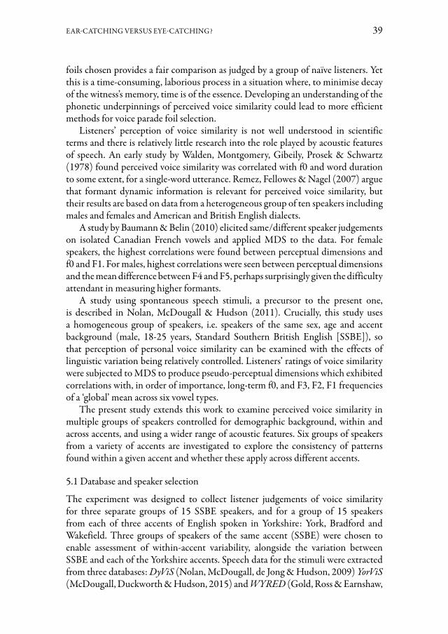
EAR-CATCHING VERSUS EYE-CATCHING? 39
foils chosen provides a fair comparison as judged by a group of naïve listeners. Yet this is a time-consuming, laborious process in a situation where, to minimise decay of the witness’s memory, time is of the essence. Developing an understanding of the phonetic underpinnings of perceived voice similarity could lead to more efficient methods for voice parade foil selection.
Listeners’ perception of voice similarity is not well understood in scientific terms and there is relatively little research into the role played by acoustic features of speech. An early study by Walden, Montgomery, Gibeily, Prosek & Schwartz (1978) found perceived voice similarity was correlated with f0 and word duration to some extent, for a single-word utterance. Remez, Fellowes & Nagel (2007) argue that formant dynamic information is relevant for perceived voice similarity, but their results are based on data from a heterogeneous group of ten speakers including males and females and American and British English dialects.
A study by Baumann & Belin (2010) elicited same/different speaker judgements on isolated Canadian French vowels and applied MDS to the data. For female speakers, the highest correlations were found between perceptual dimensions and f0 and F1. For males, highest correlations were seen between perceptual dimensions and the mean difference between F4 and F5, perhaps surprisingly given the difficulty attendant in measuring higher formants.
A study using spontaneous speech stimuli, a precursor to the present one, is described in Nolan, McDougall & Hudson (2011). Crucially, this study uses a homogeneous group of speakers, i.e. speakers of the same sex, age and accent background (male, 18-25 years, Standard Southern British English [SSBE]), so that perception of personal voice similarity can be examined with the effects of linguistic variation being relatively controlled. Listeners’ ratings of voice similarity were subjected to MDS to produce pseudo-perceptual dimensions which exhibited correlations with, in order of importance, long-term f0, and F3, F2, F1 frequencies of a ‘global’ mean across six vowel types.
The present study extends this work to examine perceived voice similarity in multiple groups of speakers controlled for demographic background, within and across accents, and using a wider range of acoustic features. Six groups of speakers from a variety of accents are investigated to explore the consistency of patterns found within a given accent and whether these apply across different accents.
5.1 Database and speaker selection
The experiment was designed to collect listener judgements of voice similarity for three separate groups of 15 SSBE speakers, and for a group of 15 speakers from each of three accents of English spoken in Yorkshire: York, Bradford and Wakefield. Three groups of speakers of the same accent (SSBE) were chosen to enable assessment of within-accent variability, alongside the variation between SSBE and each of the Yorkshire accents. Speech data for the stimuli were extracted from three databases: DyViS (Nolan, McDougall, de Jong & Hudson, 2009) YorViS (McDougall, Duckworth & Hudson, 2015) and WYRED (Gold, Ross & Earnshaw,

40 KIRSTY MCDOUGALL
2018). These databases all use the elicitation techniques developed for the DyViS database and provide spontaneous speech material for male speakers of the same age group (18-25 years for DyViS and YorViS; 18-30 years for WYRED). Each group of 15 speakers was chosen randomly from the appropriate database, with any speaker who impressionistically sounded particularly unusual being discarded from the selection. The speakers selected are shown in Table 1.
Table 1 - Speaker groups used in the experiment (speaker numbers from each database)
Group Database Speakers
SSBE1 DyViS 25, 28, 39, 53, 56, 60, 62, 65, 88, 95, 106, 111, 112, 115, 118SSBE2 DyViS 1, 2, 4, 11, 21, 23, 31, 32, 35, 37, 47, 50, 76, 87, 113SSBE3 DyViS 6, 19, 30, 40, 46, 54, 58, 68, 69, 75, 80, 81, 96, 99, 107
York YorViS 1, 2, 4, 7, 8, 10, 11, 12, 16, 17, 18, 19, 20, 21, 22Bradford WYRED 72, 132, 135, 147, 156, 157, 167, 170, 174, 175, 176, 185, 187, 189, 191Wakefield WYRED 103, 111, 112, 127, 131, 138, 141, 143, 145, 146, 152, 158, 164, 166, 178
5.2 Stimuli and experimental set-up
Stimuli were constructed from the telephone call task (Task 2) in each of the speech databases. This is a telephone conversation between the participant in the role of ‘suspect’ and his ‘accomplice’ (a researcher), in which they discuss the detail of the police interview that the participant has just undertaken, in order to ensure that the accomplice does not provide conflicting information if he is also questioned. For each ‘suspect’ participant, two speech stimuli of approximately three seconds duration were created, the first (U1) containing speech in which the participant denies knowing a man called Robert Freeman, and the second (U2) involving the participant denying having visited the Yewtree Reservoir on Wednesday evening.
Within each group of 15 speakers, each speaker was paired with himself and all other speakers to form 120 pairings. A stimulus was prepared for each pairing, containing a randomly assigned U1 and U2, separated by a silence of one second. The order in which the two utterances appeared to listeners was randomly determined, as was the ordering of the stimuli. The experiment required listeners to rate the (dis)similarity of all pairings of speakers within one of the six groups, using a Likert scale.
Listener responses for the DyViS 1 and YorViS groups were collected in person using the ‘ExperimentMFC’ (Multiple Forced Choice) facility in Praat (Boersma, Weenink, 1992-2021). The experiment was conducted in a silent sound-treated room, with participants listening via headphones. The responses to the DyViS 1 stimuli were part of an earlier experiment in which judgements were also made on telephone-recorded utterances (see Nolanet al., 2011; Nolan, McDougall & Hudson, 2013); analysis of responses to studio-recorded stimuli only are presented here. Responses to the YorViS stimuli were also collected for an earlier experiment (McDougall, Hudson & Atkinson, 2014).

EAR-CATCHING VERSUS EYE-CATCHING? 41
Responses to the DyViS 2 and DyViS 3 stimuli were collected in person using the open source software OpenSesame (Mathôt, Schreij & Theeuwes, 2012). Participants listened to stimuli over headphones in quiet laboratory rooms.
Due to the Covid-19 outbreak, the WYRED 1 and WYRED 2 stimuli sets were presented to participants online using the web-based platform Gorilla (Anwyl-Irvine, Massonnié, Flitton, Kirkham & Evershed, 2020). These participants undertook a test to check that they were using headphones or earphones (Woods, Siegel, Traer & McDermott, 2017) at the start of the experiment. Participants were allowed to take this test a second time if they did not pass it the first time.
In both the in-person and online environments, each listener was asked to judge the degree of similarity of the voices in each voice pairing, taking into account voice quality and accent, but ignoring the meaningful content of the speech. To familiarise them with the experimental set-up, listeners were given a preliminary test containing several example trials before the main test. For each stimulus pair, the screen displayed the question ‘How similar are these voices?’ and listeners were required to click a response on a Likert scale from 1 (very similar) to 9 (very different) before moving on to the next stimulus pair. Listeners were asked to give an immediate reaction and not agonise over comparisons, but the timing of each decision was under their control.
5.3 Listeners
120 listeners (20 per speaker group) took part in the experiment. They were recruited at the University of Cambridge, Nottingham Trent University and via the experimental participant recruitment website Prolific (https://www.prolific.co/). Listeners were first-language English speakers, and had been born in and lived most of their pre-18 lives in England. They were aged 18-40 years and self-reported no hearing loss or hearing difficulties. The listener group was approximately half male and half female.
5.4 Acoustic Analysis
5.4.1 Long-term fundamental frequencyLong-term fundamental frequency (f0) measures were calculated for each speaker using the 6 seconds of speech provided by the two experimental stimuli per speaker. Periods of silence and low threshold noise were removed from the files, along with any intrusive noises (coughs, furniture noises, etc.), before running the long-term pitch analysis Praat script to generate f0 statistics for each speaker.
5.4.2 Long-Term Formant analysisLong-Term Formant (LTF) analysis can be used to capture a speaker’s overall formant behaviour, by focussing on the long-term tendencies of each main formant rather than looking at individual vowel categories (Moos, 2010; Nolan, Grigoras, 2005). Frame-by-frame analyses through the voiced sections of a sample of speech are made using a formant tracker. In the present experiment, LTF analyses were

42 KIRSTY MCDOUGALL
carried out for each speaker using the Task 2 recordings. Formant-bearing speech material was manually segmented in a Praat TextGrid until 30 seconds net speech had been compiled for each speaker. This process involved a combined auditory and acoustic approach, inspecting the spectrogram while reviewing the material auditorily. Only speech material with a clear and visible formant structure for the first three formants was selected. Approximants were included, and laterals, nasals and speech exhibiting strong nasality were excluded. Vowels were excluded if they were produced with a very high pitch such that harmonics rather than formants were visible. Filled pauses were included if they were vocalic. The segmented material was subjected to formant analysis using the Snack Sound Toolkit (Sjölander, 1997). Four tracked formants were obtained for each frame in the material with an LPC order of 12, a maximum analysis frequency of 5000 Hz, a 20 ms frame length, a 10 ms frame advance and the remaining settings at their default values. This analysis achieved stable profiles for the first four formants for all but five speakers whose results have not been included (DyViS 1: 53; DyViS 2: 113; DyViS 3: 107; WYRED 1: 132, 156). The mean value of each of F1-F4 for each speaker was calculated.
5.4.3 Articulation rateArticulation rate (AR) was measured for each speaker using speech material from Task 2 following Jessen’s (2007) procedure for calculating ‘global’ AR. For each speaker, 30 ‘memory stretches’ of 5-20 syllables were analysed, with syllables determined auditorily. The syllable count for a particular utterance was defined as the actual number of syllables heard by the analyst, not the ‘canonical’ number that might be given for the entry for the same word(s) in a pronunciation dictionary. A ‘memory stretch’ was defined as a portion of fluent speech that can be retained in short-term memory of the analyst in order to count the number of phonetic syllables present ( Jessen, 2007: 54). Global AR was determined by taking the mean AR across memory stretches.
5.5 Statistical Analysis
Listeners’ similarity judgments on the voice pairs were subjected to MDS using INDSCAL (Individual Differences Euclidean Distance Model) in SPSS, with a separate analysis for each 15-speaker group. For each group, the analysis with five perceptual dimensions was chosen according to Giguère’s (2006) guideline thresholds for stress (DyViS 1: stress = 0.174, R2 = 0.277; DyViS 2: stress = 0.177, R2 = 0.171; DyViS 3: stress = 0.181, R2 = 0.145; YorViS: stress = 0.183, R2 = 0.166; WYRED 1: stress = 0.181, R2 = 0.210; WYRED 2: stress = 0.198, R2 = 0.277). Each speaker was thus characterised along five pseudo-perceptual dimensions within a perceptual space for his group of speakers with a set of five coordinates (dim1, dim2, dim3, dim4, dim5). As an example, Figure 1 gives a plot of the first two dimensions from the analysis for the SSBE 1 group, showing the 15 speakers’ locations along these dimensions. Speakers who appear relatively close on this plot were judged to be more similar-sounding (e.g. D39 and D60), while speakers who are further apart were

EAR-CATCHING VERSUS EYE-CATCHING? 43
judged less similar (e.g. D53 and D95). Each dimension accounts for successively less variance, so the lower the dimension the greater the amount of variance explained.
Figure 1 - Plot of the first two dimensions (of five) produced by the MDS analysis for the SSBE 1 group, showing the relative positions among the 15 speakers
5.6 Results
Pearson’s formula was used to test the extent of correlation between the MDS dimensions from the voice similarity ratings and the set of acoustic features measured (f0, LTF1-4, AR) for each speaker group. The absolute values of correlation coefficients which were significant (p < 0.05) are shown in Figure 2.
Figure 2 - Significant correlations (absolute value) between the acoustic features tested and the five pseudo-perceptual dimensions generated by the listeners’ voice
similarity judgements by the MDS analysis for each speaker group, dimensions 1 to 5, labelled dim1, dim2, etc.

44 KIRSTY MCDOUGALL
Long-term f0 plays a role in judgements of voice similarity in all groups except SSBE1. LTF results show significant correlations in different groups in different ways. LTF1 is significantly correlated with at least one dimension for all groups except Wakefield. LTF2 appears for two SSBE groups (1 and 3), York and Bradford. The higher formants yield a significant correlation for one group each only: in Wakefield for LTF3 and in SSBE2 for LTF4, for dim4 in both cases. AR does not play much of a role in these results, achieving significance in a higher dimension in only two of the groups: SSBE3 (dim4) and York (dim5). Within the three SSBE groups, results show some patterns, but not complete consistency. LTF1 is the only feature appearing for all three groups. The groups for the three Yorkshire accents all display a significant result for f0 in a low dimension, but differ in patterns of significance for LTF and AR features.
5.7 Discussion
Long-term f0 clearly makes an important contribution to listeners’ assessment of voice similarity, showing significant correlations in all groups except SSBE1, and generally in low dimensions. It is not surprising that f0 is dominant, given that the pitch of a voice is intuitively salient. Long-term formants are also playing a role here, correlating with dimensions 2-5 in different ways in each group, notably with F1 featuring for all groups except Wakefield. These findings of f0 being the most important and formants also making a contribution are broadly consistent with the initial Nolan et al. (2011) study (whose listener ratings are also those used for SSBE1 in the present study), although the use of ‘global’ formant measures across vowel categories rather than LTF has obviously led to some differences. The use of the INDSCAL version of MDS in the present analysis would account for the different correlation results for f0 in SSBE1 in Nolan et al. (2011).
AR appears to make some contribution to voice similarity judgements in SSBE3 and York, but needs further investigation. Given that the stimuli were only 3s in duration, it is possible that a perceptual correlate of AR had not had sufficient opportunity to become established when listeners made their decisions. Further research looking at whether temporal-based features such as AR contribute more to the perception of voice similarity for longer stretches of speech is needed.
The data collected enable variation within and across accent groups to be evaluated. The three SSBE groups yielded similar, but not identical, patterns in the profile of acoustic features correlating with perceived voice similarity. The three Yorkshire accents produced a consistent result for f0, but differences in the patterning of LTF and AR. Although the three Yorkshire groups were labelled by their three different locations, further analysis is needed to determine how perceptually different these three accents are. Looking across the six groups, it is not clear if some of the differences observed could be attributed to speaker to speaker or sample to sample variability as much as accent grouping.
A likely source of variation in the listeners’ judgements is that of their own accent background (cf. Clopper, Pisoni, 2006; Williams, Garrett & Coupland, 1999).

EAR-CATCHING VERSUS EYE-CATCHING? 45
The listeners recruited were English speakers from England, with no more specific control on their accent background; further work should investigate regional accent background of listeners as a variable.
Developing a model of perceived voice similarity that could predict how similar two voices would sound on the basis of their phonetic properties would appear to be some way off at this stage, although it is clear that f0 and formant frequencies will have a part to play. Such a model could be central to the more efficient selection of foil voices for voice parades. A further interesting future direction for this work will be to consider possible relationships between listener-assessed and machine-assessed voice similarity using automatic speaker recognition technology (see Gerlach, McDougall, Kelly, Alexander & Nolan, 2020).
6. Study 2: The effect of parade sample duration on voice recognition accuracy3
The Home Office procedure for collecting earwitness identification evidence has been implemented effectively for a number of cases in the UK since its introduction. However, there are aspects of the procedure which were devised on the basis of the parallel eyewitness procedure from Code D of PACE that have not been subjected to rigorous experimental testing in the earwitness context. For example, the procedure calls for a line-up of nine voices, but does a nine-sample parade afford optimal earwitness recognition (cf. Bull, Clifford, 1999; Levi, 1998)? The witness is asked for a decision after listening to all voices: does this serial format lead to optimal recognition, or would having the opportunity to select or reject each voice immediately after hearing the sample yield greater accuracy of recognition (cf. Seale-Carlisle, Mickes, 2016; Smith, Bird, Roeser, Robson, Braber, Wright & Stacey, 2020)? The witness is allowed to listen to each voice sample as many times as they wish: does this provide the best opportunity for a witness to recognise a voice (cf. Pozzulo, Lindsay, 1999 regarding elimination line-ups), or could interference be at play (cf. Stevenage, Howland & Tippelt, 2011)? Further, some parameters of the procedure were chosen relatively arbitrarily and would benefit from experimental examination. For example, the procedure stipulates that the voice samples should be one minute in duration, which means that the parade will be nine minutes long: does this give the witness the optimum opportunity to recognise a voice if they have heard it previously, or is this task too long and distracting (cf. Smith et al., 2020)?
One of the key aims of the IVIP project is to consider the parameters of the Home Office procedure further, and in particular to determine experimentally whether there are aspects of the procedure which could be modified to optimise the performance of earwitnesses when undertaking a voice parade. In the present paper, the results of the first IVIP experiment investigating voice parade parameters are presented: a study of the effect of voice parade sample duration on earwitness identification accuracy.
3 The description of this study given here is an overview of the findings of a larger study within IVIP, reported in greater depth in Pautz, Smith, Müller-Johnson, Nolan, Paver and McDougall (submitted).

46 KIRSTY MCDOUGALL
Little previous work is available exploring whether earwitness performance is affected by the length of the samples used in a voice parade. One exception is a study by Smith et al. (2020) which investigated earwitness accuracy for parades run with 15s or 30s voice samples. The results did not show an effect of sample duration, but research is still needed to compare the currently recommended 60s with shorter sample durations, as is investigated in the present study.
6.1 Experiment design and speaker selection
Participants were exposed to a target voice for 60s and later attempted to recognise the voice of the ‘perpetrator’ whom they heard from a target-present or target-absent voice parade. A target-present parade simulates a situation where the guilty suspect has been apprehended, whereas a target-absent parade simulates an innocent suspect having been apprehended. The same three speech databases used in Study 1 above provided the speakers in the present experiment. Voice parades were constructed for six male target speakers of English: three speakers of SSBE (from DyViS) and one of each of York (YorViS), and Bradford and Wakefield (WYRED) Englishes. These target speakers were chosen as one each from the six groups of 15 speakers used in Study 1. For each target speaker, the other 14 speakers in his group were candidates for his corresponding target-present and target-absent voice parades. Using the MDS results from Study 1, the foils for each target-present parade were chosen as the eight speakers judged by the listeners as most similar-sounding to the relevant target speaker (cf. McDougall et al., 2015). The speakers chosen for each target-absent parade were the nine speakers judged most similar-sounding to the target speaker to whom the listeners had been exposed. The speakers used as targets and foil speakers are listed in Table 2.
6.2 Speech materials
The exposure material for each target speaker was taken from Task 2, the telephone call task, in each of DyViS, YorViS, and WYRED. A sample of 60s duration was selected for each target from his side of the phone call in studio quality, with only the target’s speech included.
Table 2 - Target speakers and their corresponding foil speakers (speaker numbers from each database). * indicates the additional foil used in target-absent parades
Group Accent Target Foils
SSBE1 DyViS 56 (D1) 25*, 28, 39, 60, 65, 95, 111, 112, 115SSBE2 DyViS 23 (D2) 2, 4, 37, 31, 32, 35, 50, 76*, 87SSBE3 DyViS 80 (D3) 6, 30, 40, 46, 75, 81, 96, 99*, 107
York YorViS 8 (YO) 1*, 2, 4, 7, 8, 10, 16, 18, 19, 21Bradford WYRED 185 (W1) 187, 175, 170, 176*, 132, 189, 157, 156, 135Wakefield WYRED 166 (W2) 103*, 127, 138, 141, 145, 146, 152, 158, 178

EAR-CATCHING VERSUS EYE-CATCHING? 47
The voice parades were constructed using the Home Office (2003) methodology, using the Task 1 simulated police interview task from each database as the source of speech material. Short, self-contained chunks of speech containing words, phrases or short sentences were excised from each speaker’s interview. The parade samples were created by jumbling the order of each speaker’s chunks to form a ‘collage’ of speech giving an overall impression of that speaker’s voice. 15s, 30s and 60s voice samples were compiled for each of the speakers in the parades. Each listener undertook a parade containing either 15s, 30s or 60s samples. Allocation of listeners to one of the six target speakers within each of the six conditions (3 Sample Duration × 2 Target Presence) was done using a balanced randomisation procedure.
6.3 Experiment platform and format
The experiment was conducted online using the web-based platform Gorilla (Anwyl-Irvine et al., 2020). At the start of the experiment, participants took a test to check that they were using headphones or earphones (Woods et al., 2017). Participants were allowed to take this test a second time if they failed the first.
After listening to the 60s sample of exposure material, participants undertook a word-search task containing words for types of fruit (http://www.wordsearch-puzzles.co.uk) lasting five minutes. To prevent auditory rehearsal of the encoding, the task was accompanied by a recording of ambient noise made in a public lobby featuring unintelligible speech sounds. While a five-minute retention interval is not representative of the real-world context of a genuine voice parade case, the requirements of the task at least meant that participants’ short-term memory capacity was exceeded, and long-term memory would be relied on.
Immediately before listening to the voice parade, participants were instructed that the voice that they heard in the original recording may or may not be present in the line-up (as is recommended in the Home Office guidelines); this was noted in bold lettering in the pre-parade instructions. After they had listened to the parade and prior to indicating their decision, participants were reminded once again that the voice they had heard at the beginning of the experiment might or might not have been present in the line-up. Participants listened to all nine voices before registering a decision, then they assessed how confident they were in their decision using an eleven-point scale (0-10, with 0 = ‘not at all confident’ and 10 = ‘extremely confident’).
6.4 Participants
271 participants, 136 male and 135 female, aged 18-40 years (Mean = 27.68, SD = 6.1) were recruited via the experimental participant recruitment website Prolific (https://www.prolific.co/). Participants had been born in England, had lived in England for most or all of their lives before turning 18 years, and spoke English as their first language. Participants self-reported having no hearing loss or hearing difficulties.

48 KIRSTY MCDOUGALL
6.5 Results
The percentages of correct identifications or indications of ‘not present’ made in the voice parades for each of the three parade sample durations are shown in Figure 3. Chance level is at 10%, indicated by the dotted red line. [Total number of options = 9 possible ‘identifications’ and 1 possible ‘not present’. Chance level = 100*(1/total number of options).] Each datapoint in Figure 3 represents the responses of 42-48 (Mean = 45.1) listeners.
Performance on the parades is low overall, especially in target-absent parades. Higher levels of recognition accuracy are shown for target-present than target-absent parades. A Likelihood Test for the 3 × 2 factorial design showed a significant relationship between Target Presence and accuracy of response (G2(1) = 19.47, p < 0.001), confirming that target-present parades yield higher levels of accuracy than target-absent. Neither Sample Duration (G2(2) = 0.62, p = 0.734) nor the interaction Target Presence × Sample Duration (G2(2) = 1.45, p = 0.484) showed a significant relationship with accuracy of response.
In target-present parades, descriptively-speaking the 15s samples give the best performance (45% correct), followed by the 60s samples (38% correct), then 30s samples (36% correct). However, pairwise comparisons with a Hochberg correction (Hochberg, 1988) across sample durations gave negligible evidence to support the hypothesis that substantial differences were present, both between-groups (15s versus 30s versus 60s overall) and within-groups (target-present 15s versus target-present 30s, target-absent 15s versus target-absent 30s, etc.).
Listeners’ accuracy of performance exhibits considerable variation by individual target speaker, as can be seen in Figure 4 which shows the percentages of accurate responses in the voice parades for each of the sample duration and target presence conditions for the six target speakers separately. Chance level is at 10%, indicated by the dotted red line. Each datapoint in Figure 4 is the result of the responses of only 5-9 (Mean = 7.53) listeners and within each sample duration, the accuracy of responses is very varied. For example in the 15s condition in target-present parades, participants produced a spread of results between 28.6% for both the Y and W1 targets and 75% for the D1 target. This suggests that some voices are much harder to remember than others.

EAR-CATCHING VERSUS EYE-CATCHING? 49
Figure 3 - Percentage accuracy of participants in target-present and target-absent parades for 15s, 30s and 60s conditions. Error bars show 95% confidence intervals.
The dotted red line indicates the chance level of 10% for each condition
Figure 4 - Percentage accuracy of participants in target-present (upper panel) and target-absent (lower panel) parades for 15s, 30s and 60s sample durations.
Error bars show 95% confidence intervals. The dotted red line indicates the chance level of 10% for each condition
The listeners’ assessments of their confidence in selecting the correct voice from a parade or correctly choosing ‘not present’ are shown as mean values per sample duration and target presence condition in Figure 5.
An ordinal regression model was used to investigate the relationship between the dependent variable confidence, and the independent variables of accuracy, target presence, and sample duration. Overall, there was a statistically significant, moderately strengthened, positive association between self-related confidence and accuracy (b = .54, SE = 0.25, p = 0.034). There was no statistically significant main

50 KIRSTY MCDOUGALL
effect of target presence (b = .186, SE = 0.22, p = 0.402). With the 60s sample duration as the reference, no significant difference in confidence was found between the 15s (b = 0.48, SE = 0.26, p = 0.064) and 30s (b = 0.13, SE = 0.26, p = 0.621) sample durations.
Figure 5 - Mean confidence ratings of participants in target-present and target-absent parades for 15s, 30s and 60s conditions. Error bars show 95% confidence intervals
for the condition means
6.6 Discussion
Overall recognition accuracy was low, driven in particular by false identifications in target-absent parades (Figure 3). It is hoped that this tendency could be mitigated against through using stronger warnings stressing the real-world consequences of wrongful identification (Smith, Roeser, Pautz, Davis, Robson, Wright, Braber & Stacey, submitted). Performance on the target-present parades showed higher rates of recognition accuracy, consistent with previous research. The task itself was very difficult, arguably the more so as participants were not told that their memory of the voice heard would be tested until after the retention interval had elapsed. In real-world situations, one would expect the witness’s exposure to the voice to be longer than the one minute given in the present experiment, and that the witness would have expressed some preparedness to recall the voice heard at the crime scene on a future occasion. In the present study, listeners’ confidence ratings tended to fall in the middle of the scale (Figure 5), possibly reflecting indecision, and suggesting that participants were aware of the difficulty of the identification task.
The results comparing parade sample durations presented here suggest that the Home Office procedure for voice parades could be modified by reducing parade sample duration to between 15 and 30 seconds satisfactorily. This would reduce the total amount of work needed from the phonetician preparing the samples and hence slightly speed up the process of constructing a parade. Further, the requirement for less speech material within each sample may open up the number of candidate foil

EAR-CATCHING VERSUS EYE-CATCHING? 51
recordings available when compiling a parade, since shorter interviews containing less material would become eligible for consideration.
The experimental results also highlight the importance of taking into account individual differences between target speakers. The six different target speakers used yielded markedly different levels of identification accuracy across the various experimental conditions. The recognisability of different target speakers varies greatly (cf. McDougall, Nolan & Hudson, 2015), yet many experimental studies investigating earwitness performance are conducted using a single target speaker. The use of different target speakers in the present experiment is likely to have contributed some of the noise in the comparison of conditions, yet it is crucial to appreciate the extent of variability of identification accuracy yielded by different target speakers. A key area for future research is what makes a voice more distinctive and/or memorable to listeners (cf. Sørensen, 2012), a topic being pursued in other studies within the IVIP project.
7. Concluding remarksSince earwitness evidence can make a crucial contribution to a criminal case it is essential that it is collected on the basis of a comprehensive knowledge base. Given that research shows that different mechanisms are involved in processing faces and voices, earwitness identification procedures must be developed specifically in the light of auditory-oriented research. This paper has presented two studies from the IVIP project with implications for voice parade procedures. The first offers some initial foundations for the development of a model of perceived voice similarity which could in principle contribute to the process of selecting the foils for a voice parade. The second provides support for the notion of reducing the duration of voice samples used in the voice parade procedure in England and Wales.
AcknowledgementsThanks are due to the IVIP project researchers, especially Harriet Smith, Nikolaus Pautz, Katrin Müller-Johnson, Alice Paver and Francis Nolan for their contributions to the work presented in §5 and §6. The IVIP project is funded by the UK Economic and Social Research Council [Grant Reference ES/S015965/1] and is hosted by the University of Cambridge, De Montfort University, Nottingham Trent University and the University of Oxford. The author is grateful to Philip Harrison for his assistance with LTF analysis. Further thanks are due to Nathan Atkinson, Toby Hudson, Christin Kirchhübel and Elaine Schmidt for their assistance with data collection and measurement in the earlier projects VoiceSim and YorViS upon which the IVIP project builds, and to Erica Gold for providing her AR measurements for the DyViS speakers.

52 KIRSTY MCDOUGALL
Bibliography
Anwyl-Irvine, A.L., Massonnié, J., Flitton, A., Kirkham, N. & Evershed, J.K. (2020). Gorilla in our midst: An online behavioral experiment builder. In Behavior Research Methods, 31(1), 388-407. [DOI: 10.3758/s13428-019-01237-x].Barton, J.J. (2008). Structure and function in acquired prosopagnosia: Lessons from a series of 10 patients with brain damage. In Journal of Neuropsychology, 2(1), 197-225. [DOI: 10.1348/174866407X214172].Baumann, O., Belin, P. (2010). Perceptual scaling of voice identity: Common dimensions for different vowels and speakers. In Psychological Research, 74, 110–120. [DOI: 10.1007/s00426-008-0185-z].Belin, P., Fecteau, S. & Bedard, C. (2004). Thinking the voice: Neural correlates of voice perception. In Trends in Cognitive Sciences, 8(3), 129-135. [DOI: 10.1016/j.tics.2004.01.008].Belin, P., Bestelmeyer, P.E.G., Latinus, M. & Watson, R. (2011). Understanding voice perception. In British Journal of Psychology, 102(4), 711-725. [DOI: 10.1111/j.2044-8295.2011.02041.x].Boersma, P., Weenink, D. (1992-2021). PRAAT: Doing phonetics by computer. [Computer program]. http://www.praat.org/.Brédart, S., Barsics, C. (2012). Recalling semantic and episodic information from faces and voices: A face advantage. In Current Directions in Psychological Science, 21(6), 378-381. [DOI: 10.1177/0963721412454876].Broeders, A.P.A. (1996). Earwitness identification: Common ground, disputed territory and uncharted areas. In Forensic Linguistics, 3(1), 3-13. [DOI: 10.1558/ijsll.v3i1.3].Broeders, A.P.A., Rietveld, A.C.M. (1995). Speaker identification by earwitnesses. In Braun, A., Köster, J.-P. (Eds.), Studies in forensic phonetics: Beiträge zur Phonetik und Linguistik, 64, 24-40.Bruce, V., Young, A.W. (1986). Understanding face recognition. In British Journal of Psychology, 77, 305-327. [DOI: 10.1111/j.2044-8295.1986.tb02199.x].Bull, R., Clifford, B. (1999). Earwitness testimony. In Heaton-Armstrong, A., Shepherd, E. & Wolchover, D. (Eds.), Analysing witness testimony: A guide for legal practitioners and other professionals. London: Blackstone, 194-206.Campanella, S., Belin, P. (2007). Integrating face and voice in person perception. In Trends in Cognitive Sciences, 11(12), 535-543. [DOI: 10.1016/j.tics.2007.10.001].Clopper, C.G., Pisoni, D.B. (2006). Effects of region of origin and geographic mobility on perceptual dialect categorization. In Language Variation and Change, 18(2), 193-221. [DOI: 10.1017/S0954394506060091].de Jong-Lendle, G., Nolan, F., McDougall, K. & Hudson, T. (2015). Voice lineups: A practical guide. In The Scottish Consortium for ICPhS 2015 (Ed.), Proceedings of the 18th International Congress of Phonetic Sciences, Glasgow, 10-14 August 2015, Paper number 0598. 1-5. [https://www.internationalphoneticassociation.org/icphs-proceedings/ICPhS2015/Papers/ICPHS0598.pdf ].

EAR-CATCHING VERSUS EYE-CATCHING? 53
Ellis, H.D., Jones, D.M. & Mosdell, N. (1997). Intra- and inter-modal repetition priming of familiar faces and voices. In British Journal of Psychology, 88(1), 143-156. [DOI: 10.1111/j.2044-8295.1997.tb02625.x].Garrido, L., Eisner, F., McGettigan, C., Stewart, L., Sauter, D., Hanley, J.R., Schweinberger, S.R., Warren, J.D. & Duchaine, B. (2009). Developmental phonagnosia: A selective deficit of vocal identity recognition. In Neuropsychologia, 47(1), 123-131. [DOI: 10.1016/j.neuropsychologia.2008.08.003].Gerlach, L., McDougall, K., Kelly, F., Alexander, A. & Nolan, F. (2020). Exploring the relationship between voice similarity estimates by listeners and by an automatic speaker recognition system incorporating phonetic features. In Speech Communication, 124, 85-95. [DOI: 10.1016/j.specom.2020.08.003].Giguère, G. (2006). Collecting and analyzing data in multidimensional scaling experiments: A guide for psychologists using SPSS. In Tutorial in Quantitative Methods for Psychology, 2(1), 27-38. [DOI: 10.20982/tqmp.02.1.p026].Gold, E., Ross, S. & Earnshaw, K. (2018). The ‘West Yorkshire Regional English Database’: Investigations into the generalizability of reference populations for forensic speaker comparison casework. In Proceedings of Interspeech 2018, Hyderabad, 2-6 September 2018, 2748-2752. [DOI: 10.21437/Interspeech.2018-65].Hailstone, J.C., Crutch, S.J., Vestergaard, M.D., Patterson, R.D. & Warren, J.D. (2010). Progressive associative phonagnosia: A neuropsychological analysis. In Neuropsychologia, 48(4), 1104-1114. [DOI: 10.1016/j.neuropsychologia.2009.12.011].Hochberg, Y. (1988). A sharper Bonferroni procedure for multiple tests of significance. In Biometrika, 75(4), 800-802. [DOI: 10.2307/2336325].Hollien, H. (1996). Consideration of guidelines for earwitness lineups. In Forensic Linguistics, 3(1), 14-23. [DOI: 10.1558/ijsll.v3i1.14].Home Office (2003). Advice on the use of voice identification parades. UK Home Office Circular 057/2003 from the Crime Reduction and Community Safety Group, Police Leadership and Powers Unit [http://webarchive.nationalarchives.gov.uk/20130125153221/http://www.homeoffice.gov.uk/about-us/corporate-publications-strategy/home-office-circulars/circulars-2003/057-2003/]Imaizumi, S., Mori, K., Kiritani, S., Hosoi, H. & Tonoike, M. (1997). Task-dependent laterality for cue decoding during spoken language processing. In NeuroReport, 8, 899-903. [DOI: 10.1097/00001756-199803300-00025].Jessen, M. (2007). Forensic reference data on articulation rate in German. In Science and Justice, 47, 50-67. [DOI: 10.1016/j.scijus.2007.03.003].Levi, A.M. (1998). Protecting innocent defendants, nailing the guilty: A modified sequential lineup. In Applied Cognitive Psychology, 12(3), 265-275. [DOI: 10.1002/(SICI)1099-0720(199806)12:3<265::AID-ACP515>3.0.CO;2-O].Lindsay, R.C.L., Ross, D.F., Read, J.D. & Toglia, M.P.(2007). The handbook of eyewitness psychology. Volume II: Memory for people. Mahway, NJ.: Lawrence Erlbaum.Mathôt, S., Schreij, D. & Theeuwes, J. (2012). OpenSesame: An open-source, graphical experiment builder for the social sciences. In Behavior Research Methods, 44(2), 314-324. [DOI: 10.3758/s13428-011-0168-7].

54 KIRSTY MCDOUGALL
McDougall, K. (2013). Assessing perceived voice similarity using multidimensional scaling for the construction of voice parades. In International Journal of Speech, Language and the Law, 20(2), 163-172. [DOI: 10.1558/ijsll.v20i2.163].McDougall, K., Hudson, T. & Atkinson, N. (2014). Listeners’ perception of voice similarity in Standard Southern British English versus York English. Paper presented at International Association for Forensic Phonetics and Acoustics Annual Conference, Zürich, August 31 – September 3, 2014.McDougall, K., Duckworth, M. & Hudson, T. (2015). Individual and group variation in disfluency features: A cross-accent investigation. In 2015, The Scottish Consortium for ICPhS 2015 (Ed.), Proceedings of the 18th International Congress of Phonetic Sciences, Glasgow, 10-14 August 2014, Paper number 0308.1-5. [http://www.icphs.info/pdfs/Papers/ICPHS0308.pdf ]McDougall, K., Nolan, F. & Hudson, T. (2015). Telephone transmission and earwitnesses: Performance on voice parades controlled for voice similarity. In Phonetica, 72, 257-272. [DOI: 10.1159/000439385].Moos, A. (2010). Long-term formant distribution as a measure of speaker characteristics in read and spontaneous speech. In The Phonetician, 101/102, 7-24.Neuner, F., Schweinberger, S.R. (2000). Neuropsychological impairments in the recognition of faces, voices, and personal names. In Brain and Cognition, 44, 342-366. [DOI: 10.1006/brcg.1999.1196].Nolan, F. (2003). A recent voice parade. In International Journal of Speech, Language and the Law, 10(2), 277-291. [DOI: 10.1558/sll.2003.10.2.277].Nolan, F., Grigoras, C. (2005). A case for formant analysis in forensic speaker identification. In International Journal of Speech, Language and the Law, 2(2), 143-173. [DOI: 10.1558/sll.2005.12.2.143].Nolan, F., McDougall, K. & Hudson, T. (2011). Some acoustic correlates of perceived (dis)similarity between same-accent voices. In Lee, W.-S., Zee, E. (Eds.), Proceedings of the 17th International Congress of Phonetic Sciences, Hong Kong, 17-21 August 2011, 1506-1509. [http://www.icphs2011.hk/resources/OnlineProceedings/RegularSession/Nolan/Nolan.pdf ]Nolan, F., McDougall, K. & Hudson, T. (2013). Effects of the telephone on perceived voice similarity: Implications for voice line-ups. In International Journal of Speech, Language and the Law, 20(2), 229-246. [DOI: 10.1558/ijsll.v20i2.229].Nolan, F., McDougall, K., de Jong, G. & Hudson, T. (2009). The DyViS database: Style-controlled recordings of 100 homogeneous speakers for forensic phonetic research. In International Journal of Speech, Language and the Law, 16(1), 31-57. [DOI: 10.1558/ijsll.v16i1.31].Pautz, N., Smith, H.M.J., Müller-Johnson, K., Nolan, F., Paver, A. & McDougall, K., (submitted). Identifying unfamiliar voices: the influence of sample duration and parade size. Pre-print at https://psyarxiv.com/h9ynr/Pozzulo, J.D., Lindsay, R.C.L. (1999). Elimination lineups: An improved identification procedure for child eyewitnesses. In Journal of Applied Psychology, 84(2), 167-176. [DOI: 10.1037/0021-9010.84.2.167].

EAR-CATCHING VERSUS EYE-CATCHING? 55
Remez, R.E., Fellowes, J.M. & Nagel, D.S. (2007). On the perception of similarity among talkers. In Journal of the Acoustical Society of America, 122(6), 3688-96. [DOI: 10.1121/1.2799903].Rietveld, A.C.M., Broeders, A.P.A. (1991). Testing the fairness of voice identity parades: The similarity criterion. In Proceedings of the 12th International Congress of Phonetic Sciences, Aix-en-Provence, 19-24 August 1991, 46-49.Robson, J. (2017). A fair hearing? The use of voice identification parades in criminal investigations in England and Wales. In Criminal Law Review(1), 36-50. [http://irep.ntu.ac.uk/id/eprint/29636/1/6791_Robson.pdf ].Schiffman, S.S., Lance Reynolds, M. & Young, F.W. (1981). Introduction to multidimensional scaling: Theory, methods, and applications. New York: Academic Press.Seale-Carlisle, T.M., Mickes, L. (2016). US line-ups outperform UK line-ups. In Royal Society Open Science, 3, 160-300. [DOI: 10.1098/rsos.160300].Sheffert, S.M., Olson, E. (2004). Audiovisual speech facilitates voice learning. In Perception and Psychophysics, 66, 352-362. [DOI: 10.3758/bf03194884].Sjölander, K. (1997). The Snack sound toolkit. [Computer program]. [http://www.speech.kth.se/snack/].Smith, H.M.J., Bird, K., Roeser, J., Robson, J., Braber, N., Wright, D. & Stacey, P.C. (2020). Voice parade procedures: Optimising witness performance. In Memory, 28(1), 2-17. [DOI: 10.1080/09658211.2019.1673427].Smith, H.M.J., Roeser, J., Pautz, N., Davis, J.P., Robson, J., Wright, D., Braber, N. & Stacey, P.C. (submitted). Evaluating earwitness identification procedures: Adapting pre-parade instructions and parade procedure. [Preprint https://psyarxiv.com/nxr3e/].Sørensen, M.H. (2012). Voice line-ups: Speakers’ f0 values influence the reliability of voice recognitions. In International Journal of Speech, Language and the Law, 19(2), 145-158. [DOI: 10.1558/ijsll.v19i2.145].Stevenage, S.V., Neil, G.J. (2014). Hearing faces and seeing voices: The integration and interaction of face and voice processing. In Psychologica Belgica, 54(3), 266-281. [DOI: 10.5334/pb.ar].Stevenage, S.V., Howland, A. & Tippelt, A. (2011). Interference in eyewitness and earwitness recognition. In Applied Cognitive Psychology, 25(1), 112-118. [DOI: 10.1002/acp.1649].von Kriegstein, K., Eger, E., Kleinschmidt, A. & Giraud, A.L. (2003). Modulation of neural responses to speech by directing attention to voices or verbal content. In Cognitive Brain Research, 17(1), 48-55. [DOI: 10.1016/s0926-6410(03)00079-x].von Kriegstein, K., Kleinschmidt, A., Sterzer, P. & Giraud, A.-L. (2005). Interaction of face and voice areas during speaker recognition. In Journal of Cognitive Neuroscience, 17(3), 367-376. [DOI: 10.1162/0898929053279577].Walden, B.E., Montgomery, A.A., Gibeily, G.J., Prosek, R.A. & Schwartz, D.M. (1978). Correlates of psychological dimensions in talker similarity. In Journal of Speech and Hearing Research, 21, 265-275. [DOI: 10.1044/jshr.2102.265].Williams, A., Garrett, P. & Coupland, N. (1999). Dialect recognition. In Preston, D.R. (Ed.), Handbook of perceptual dialectology. Philadelphia: John Benjamins, 345-358.

56 KIRSTY MCDOUGALL
Woods, K.J.P., Siegel, M., Traer, J. & McDermott, J.H. (2017). Headphone screening to facilitate web-based auditory experiments. In Attention, Perception & Psychophysics, 79(7), 2064-2072. [DOI: 10.3758/s13414-017-1361-2].Young, A.W., Frühholz, S. & Schweinberger, S.R. (2020). Face and voice perception: Understanding commonalities and differences. In Trends in Cognitive Sciences, 24(5), 398-410. [DOI: 10.1016/j.tics.2020.02.001].Yovel, G., Belin, P. (2013). A unified coding strategy for processing faces and voices. In Trends in Cognitive Sciences, 17(6), 263-271. [DOI: 10.1016/j.tics.2013.04.004].

DOI: 10.17469/O2108AISV000003
KATHARINA KLUG, MICHAEL JESSEN, YOSEF A. SOLEWICZ, ISOLDE WAGNER
Collection and analysis of multi-condition audio recordings for forensic automatic speaker recognition
The major aim of the project presented here is to compile a corpus from real case recordings to validate more recording conditions and languages under match and mismatch conditions for forensic automatic speaker recognition (FASR). The challenges and limitations of compiling a real case corpus are explained. First results of validation tests are presented for male speakers of German in the match condition [voice message – voice message] as well as in the mismatch condition [voice message – telephone]. Results for the match condition [voice message] are compared to previous findings for the match condition [telephone]. Variations of performance metrics such as Equal Error Rate (EER) and log-likelihood-ratio cost (Cllr) are discussed with respect to effects of normalisation and calibration, and patterns of score distributions are analysed using Tippett plots.
Keywords: Forensic automatic speaker recognition, Real case recordings, Validation, Match and mismatch condition, Calibration.
1. IntroductionThe present paper outlines a research project aiming to validate forensic automatic speaker recognition (FASR) systems by using real forensic audio recordings. With the improvement of FASR systems over the past two decades, the use of the automatic approach as an element alongside auditory and/or acoustic analysis in speaker comparison casework has increased significantly worldwide (Gold, French, 2019). Both the auditory-acoustic approach and FASR are based on Bayesian principles in assessing similarity and typicality ( Jessen 2018; Rose 2002 for the foundations of Bayesian statistics and the likelihood ratio in forensic speaker comparison). However, while FASR generates a quantitative strength-of-evidence outcome (likelihood ratio), the auditory-acoustic approach produces a more qualitative outcome. Combining both approaches would therefore increase the level of information when expressing conclusions.
Validating (i.e. testing) FASR systems is necessary to assess the case-specific strength of evidence given the specific case condition material (Drygajlo, Jessen, Gfroerer, Wagner, Vermeulen & Niemi, 2015: 17; Morrison, Enzinger, Hughes, Jessen, Meuwly, Neumann, Planting, Thompson, van der Vloed, Ypma, Zhang, Anonymous & Anonymous, 2021). So far, only a limited proportion of common forensic scenarios in cases submitted to the German Federal Criminal Police Office

58 KATHARINA KLUG, MICHAEL JESSEN, YOSEF A. SOLEWICZ, ISOLDE WAGNER
(Bundeskriminalamt, BKA) has been validated, i.e. [telephone]1 conversations of male speakers of German. Accordingly, the rate of FASR application in casework is low. Within the last 15 years only 10-20% of conducted speaker comparison cases at the BKA have met the requirements for FASR application. These requirements include sufficient recording quality and quantity of speech, and consistency in terms of spoken language and recording condition. Over the last five years, the percentage of FASR-treated speaker comparison cases actually decreased. Possible reasons for the reduction could be the change in submitted recording material from predominantly [telephone] recordings to different types of recordings (e.g. voice messages, videos, interior surveillance). The vast majority of scenarios, i.e. languages and recording conditions, and in particular the various combinations of mismatch situations, have not been tested yet. The present research project starts to fill this gap by compiling a corpus consisting of speakers of various languages and recording conditions in match and mismatch settings.
However, given the vast number of potential combinations of mismatch scenarios that forensic speech experts might face, the present project is merely a starting point. The collection of real forensic audio recordings needs to be continuously expanded to fully exploit the capability of such a real case corpus. Due to restrictions in data availability and data access this remains the main challenge for validating FASR on real forensic audio recordings.
2. Mismatch conditions and unfamiliar match conditionsMismatch factors can be manifold. Kelly, Hansen (2021) subdivide (1) extrinsic and (2) intrinsic factors, which are either (1) speaker-independent (e.g. background noise, transcoding effects, channel characteristics, recording devices) or (2) speaker-dependent (e.g. emotional or stylistic variation, vocal effort, short- or long-term voice fluctuations as in the case of a cold or ageing effects). Due to this diversity, more than one mismatch factor can appear at the same time, leading to ‘multi-mismatch’ scenarios. In fact, multi-mismatch is inevitable in forensic speaker comparison cases and, furthermore, the ground truth of many mismatch factors, such as transcoding history, recording hardware and software, date of origin, can only be estimated.
Previous FASR studies investigated the effects of individual types of mismatch using controlled and/or manipulated data (e.g. Nash, 2019; Kelly, Hansen, 2021). Such simulated test corpora are necessary to arrive at generalisations as the data’s ground truth is known and potential further factors can be kept as similar as possible to investigate only one factor at a time. Factors which have been studied so far include but are not limited to: mismatch in spoken language (Künzel, 2013), mismatch in time span between recordings of interest (Morrison, Kelly, 2019), mismatch in acoustics (net speech duration, signal-to-noise ratio, reverberation,
1 In this paper, the conditions tested using FASR are listed in square brackets.

COLLECTION AND ANALYSIS OF MULTI-CONDITION AUDIO RECORDINGS 59
frequency bandwidth and transcoding) (Nash, 2019), mismatch in recording device (van der Vloed, Kelly & Alexander, 2020) and mismatch in vocal effort (Kelly, Hansen, 2021).
Nash (2019) studied the effect of net duration on discrimination performance and found that lower net duration led to lower same-speaker (subsequently abbreviated as SS) scores and higher different-speaker (DS) scores, while system accuracy decreased (p. 126). Testing the effect of net duration in match and mismatch conditions using an i-vector/PLDA system he found that down to a performance tipping point of 10 seconds the discrimination performance decreased gradually. Net durations below 10 seconds, however, resulted in an exponential performance degradation. Mismatch in net duration does not seem to have an impact on the Equal Error Rate (EER), i.e. discrimination performance was not systematically improved by matching the net duration of the recordings to be compared. According to Nash’s results, EERs increased when net durations decreased from 25s, over 20s to 10s, even though they matched in duration for each of these steps. But, for example, having a pair of recordings with one of them 10s long and the other 30s (duration mismatch) led to better average performance than matching both recordings at a value of 10s. Duration might be the only variable that behaves in this manner. Usually, a mismatch in conditions led to poorer performance than a match. For example, a mismatch between noise-free and noise-degraded speech is worse than a match between two equally noise-degraded recordings.
Beyond mismatch, a further issue is the behaviour of “unfamiliar” match conditions. The classifier “unfamiliar” refers to types of intrinsic factors, extrinsic factors, or combinations of the two which are scarcely represented in the literature and have not been sufficiently tested yet (at the BKA, Israel Police or other forensic services). In contrast to mismatch, here conditions are matched but unfamiliar (i.e. same but unfamiliar condition for the questioned speaker as well as for the suspected speaker). Forensically, the question arises whether a test (validation) that has been conducted for Condition A also applies to Condition B, i.e. whether the results for the two conditions are very similar (e.g. Solewicz, Jessen & van der Vloed, 2017 for strong similarity between a Dutch-based and a German-based test), or whether at least some process of interpolation or extrapolation can be applied in order to bridge the two (Morrison, Kelly, 2019 for an example of interpolation).
To give an example of unfamiliar match conditions, Nash (2019) investigated the effect of transcoding using controlled data of twelve different codec types with various settings. Lossy codecs in particular, relying on psychoacoustic compression, influenced the discrimination rate considerably and increased the rate of false rejections and false acceptances (p. 264). Formats typically involved are MP3, M4A and AAC. Nash hypothesised that recordings from the same codec would artificially increase discrimination performance due to a match in channel characteristics (p. 256). This means that a match among unfamiliar

60 KATHARINA KLUG, MICHAEL JESSEN, YOSEF A. SOLEWICZ, ISOLDE WAGNER
conditions might lead to overconfident results – a pattern that will become relevant in this study.
A recent study on both mismatch and unfamiliar match conditions was carried out by Kelly, Hansen (2021). They studied the impact of vocal-effort variation using [whisper], [Lombard] speech and [neutral] speech to assess mismatch in vocal effort. They found, using an x-vector system, that both mismatch conditions [whisper – neutral] and [Lombard – neutral] lowered discrimination performance; however, more so when [whisper] was involved (EER of ≈ 20%) rather than [Lombard] speech (EER of max 3.62%). Considerably better discrimination performance was found for [non-neutral] match comparisons, i.e. [whisper – whisper] (EER of max 7.36%) and [Lombard – Lombard] (EER of max 2.12%). Thus, the match conditions in vocal effort – even though they are based on [non-neutral] speech – outperformed the mismatch situation.
The above studies allow the effects of individual factors to be assessed under controlled conditions. However, given that controlled data produce very homogeneous scenarios, the results obtained should be considered as more optimistic than expected for typical forensic scenarios in which factors of interest do not occur in isolation. Therefore, as Drygajlo et al. (2015: 17) demanded, FASR systems need to be validated using corpora that match casework conditions, if possible, by using available data from previous casework. In the casework-based paper presented here, the mismatch condition was [voice message] against [telephone] communication and the “unfamiliar” match condition was [voice message]. For the mismatch condition it is interesting to see how performance changed (probably decreased) relative to a [voice message] match condition. For the match condition based on [voice message] data, a comparison was made to a previously used [telephone] interception corpus (Solewicz et al. 2017) and the question was whether performance is similar in these two match condition datasets. “Performance” not only concerns speaker discrimination or calibration values, but also the actual distributions of the scores in Tippett plots, which are expected to reveal further interesting patterns.
3. The FORBIS projectThe FORBIS project (short for Collection and analysis of recordings for FORensic BIometric Speaker recognition) is a research project funded by the EU Internal Security Fund and was conducted at the BKA from March 2019 to August 2021. The project’s main goal was to compile a corpus of recordings suitable for FASR validation tests to enable the application of FASR for additional recording conditions and further spoken languages beyond the hitherto focus on German telephone data. The basis for the compilation of the corpus was the archive of the BKA section ‘Text, speech and audio’, from which suitable recordings were collected. In addition, other BKA divisions were asked to provide real forensic audio and video material from investigative proceedings.

COLLECTION AND ANALYSIS OF MULTI-CONDITION AUDIO RECORDINGS 61
3.1 Corpus limitations
Potential extrinsic and intrinsic factors, causing multi-mismatch, should be considered when compiling a corpus based on real case recordings. The following list shows some examples of relevant factors (for a more complete collection see Hansen, Bořil, 2018).Extrinsic factors:– Recording quantity: net speech duration– Recording quality: effects of recording and transmission procedures, i.e. linear
and non-linear distortions– Background noise, e.g. traffic, babble, wind noiseIntrinsic factors:– Emotional state– Speaking style– Vocal effort– Time span between recordings
Because the actual basis, i.e. the ground truth, of many factors remained unknown (e.g. how the recording was transmitted exactly, or if a speaker was indeed emotional), evaluating the impact of individual factors was complicated. Further difficulties were caused by various imbalances, namely the number of recordings per speaker, the number of speakers per recording condition (e.g. telephone intercept, voice message) and the number of speakers per language. As for any collection of forensically authentic recordings, there was also a remaining uncertainty about speaker identities, i.e. correct assignment of SS and DS status in the validation dataset.
3.2 Corpus compilation
Only recordings of male speakers were collected. In addition to German, the languages Arabic, Turkish and Russian most frequently appeared in casework at the ‘Text, speech and audio’ section of the BKA in recent years and thus were included in the corpus. Typically, the following four recording conditions were submitted for speaker comparison purposes and thus required validation tests: [telephone] interception, [voice message], [video] and [interior surveillance] (both indoor and car surveillance). To prevent the dominance of a few speakers, the maximum number of recordings per speaker was limited to six recordings per language and condition. In general, the aim for the corpus was to arrive at a minimum of 20 speakers for each language and recording condition. In addition to the recordings collected for creating a test set, matching reference populations were needed for normalisation purposes within the FASR system used (addressed in § 4). The aim was to collect 30 additional speakers with one recording per speaker for each language and each recording condition.

62 KATHARINA KLUG, MICHAEL JESSEN, YOSEF A. SOLEWICZ, ISOLDE WAGNER
4. FASR system and performance testingThe FASR system VOCALISE (VOice Comparison and Analysis of the LIkelihood of Speech Evidence) Version 2.7 (Kelly, Forth, Kent, Gerlach & Alexander, 2019a for further information) was used to conduct the speaker recognition tasks (i.e. speaker comparisons) based on Mel Frequency Cepstral Coefficients (MFCCs). Pre-tests showed that the state-of-the-art x-vector PLDA system based on DNN embeddings outperformed the previous i-vector PLDA system. According to recommendations by the developers x-vectors were supposed to improve system performance under mismatch conditions and when degraded recordings were used. The results presented here were taken from the x-vector system only. Bio-Metrics Version 1.8 was used for examination of the system’s discrimination and calibration performance (Equal Error Rate, EER, and log-likelihood-ratio cost, Cllr), visualisation of the score distributions (Tippett plots), implementation of cross validation calibration (CV) and Zoo plots.
Various system options were tested individually as well as in combination, revealing the system’s raw scores [-norm, -CV], normalised scores [+norm, -CV] as well as calibrated scores for both, raw scores [-norm, +CV] and normalised scores [+norm, +CV]. “Score Normalisation” (henceforth “normalisation”) was applied using S-norm (symmetric normalisation, Shum, Dehak, Dehak & Glass, 2010). The details of the normalisation procedure in VOCALISE are described in Kelly et al. (2019a). Essentially, the recordings used in the test were compared with recordings of a set of speakers unrelated to the test data but with equivalent speaking conditions. Means and standard deviations of the score results of these comparisons were calculated and used to shift the score result of each comparison in the test. Generally, normalisation has the effect of improving discrimination performance to some extent, which is the main motivation for its use.
Calibration was applied using logistic regression cross validation calibration. Calibration has the goal of turning the raw scores into interpretable likelihood ratios, which means that if expressed in terms of LLR (log likelihood ratios) values larger than zero are typical for SS comparisons and values smaller than zero are typical for DS comparisons. The logistic regression calibration technique calculates shift and scale parameters from a calibration dataset and applies them to the scores. Cross validation is a “leave-one-out” method. The same corpus is used both for training the calibration parameters and for testing, but the speaker(s) involved in each comparison cycle is/are removed from the training set. For further literature on EER, Cllr, Tippett plots, logistic regression calibration and the cross validation principle see van Leeuwen, Brümmer (2007), Morrison (2011), Morrison (2013) and Drygajlo et al. (2015).
5. Speech dataValidation tests were performed on recordings of German speakers in the match condition [voice message], as well as in the mismatch condition [voice message –

COLLECTION AND ANALYSIS OF MULTI-CONDITION AUDIO RECORDINGS 63
telephone] interception. Available material gained from the FORBIS corpus was fully exploited. The material used for the tests is summarised in Tab. 1. The target criteria for the number of speakers could be met for the match condition (20 speakers), but not for the mismatch condition. Only recordings of 7 speakers could be collected in both conditions: [voice message] and [telephone] interception. For the reference population, recordings of 15 additional speakers from the [voice message] condition could be collected. For the mismatch condition, recordings of another 15 speakers from [telephone] interceptions were used. Consequently, the reference population for the mismatch condition was balanced for both conditions, as is the recommended procedure when using S-norm under mismatch conditions.
5.1 Pre-tests
Transcoding formats based on psychoacoustic compression (e.g. MP3, AAC) are known to degrade discrimination performance using controlled data (Nash, 2019). Pre-tests confirmed these results. Recordings transcoded in MP3 or AAC format produced some outliers. The OPUS format, also available in high quality, did not show such an effect. However, this impression is based on only 23 OPUS files in the match corpus and 6 OPUS files in the mismatch corpus.
Originally, the corpus creation aimed at maximising the number of speakers and the number of recordings per speaker. Therefore, a rather permissive selection process was applied in terms of suitable recording formats, recording quality and neutral speaking style. Accordingly, the system performance in terms of EER of the original test set was quite poor.
The following types of recording degradations were identified in the pre-tests as causing lower system performance and were therefore removed from the test set:– Reduced frequency bandwidth– Unsteady sound pressure level, i.e. clipping and reduction– Data loss due to transcoding– Non-neutral speaking style, e.g. emotional, fatigue, intoxicatedThe exclusion of recordings was based on auditory and acoustic examination. Despite excluding poor and non-neutral recordings, the compiled test set (Tab. 1) still contained different kinds and degrees of degradation causing random effects of mismatch. This, however, is typical of casework data.
For data used in the mismatch test, a slight tendency was observed that there was a greater proportion of quality degradation in the [voice message] recordings than in the [telephone] recordings. The quality degradations were in-vehicle noise, background speakers and reverberation, all of which were either absent or present to a lower degree in the [telephone] recordings. This tendency will become relevant when interpreting the results.
The recordings compiled for the test sets also underwent a screening process using Zoo plots (see Dunstone, Yager, 2009). In the data set intended for the mismatch test, one outlier in the form of a “phantom” was observed. Phantoms are

64 KATHARINA KLUG, MICHAEL JESSEN, YOSEF A. SOLEWICZ, ISOLDE WAGNER
speakers that show an unusually low similarity (in terms of LLRs) when compared to other speakers and also when compared to themselves, i.e. across recording of the same speaker. That phantom-type speaker was the only one among the seven who was classified as non-normal in the Zoo plots; this status stayed the same across the four conditions [-norm, -CV], [-norm, +CV], [+norm, -CV] and [+norm, +CV]. Rather than excluding that speaker from analysis altogether, two separate types of tests were performed, one in which that speaker (referred to as “P”) was included (see third column in Tab. 1) and one in which he was excluded (see last column). This seemed advisable given the number of available speakers was quite small from the start.
Table 1 - Test sets for match and mismatch condition
Number of Match Mismatch Mismatch without speaker P
Speakers 20 7 6Recordings 62 34 29
SS comparisons 42 39 33DS comparisons 798 246 175
Ref. population
speakers
15(all voice messages)
30(balanced for both
rec. condition)
30(balanced for both
rec. condition)
6. MethodologyEach recording was converted into a PCM WAV format (44.1 kHz, stereo) using an in-house audio converter. All files were downsampled to 8 kHz using Praat (Boersma, Weenink, 2016) as only frequencies up to 4 kHz are used for MFCC extraction (Kelly, Fröhlich, Dellwo, Forth, Kent & Alexander, 2019b). The channels with the speakers of interest were extracted and the relevant net speech was manually labelled and extracted using the TextGrid and script function within Praat. The main criterion for speech labelling was based on intelligibility. Only neutral speech was labelled while interferences and extreme occurrences of non-neutral speech were discarded, e.g. disturbing noise, further speakers in one-channel recordings, non-neutral phonation types (falsetto, whisper), highly increased vocal effort (screaming etc.), laughing. Net speech editing included the manual removal of pauses; VAD (voice activity detection) was therefore disabled in VOCALISE for the purpose of the tests. Nash (2019: 259) observed a cliff edge effect for recordings with net duration lower than 10 seconds. Especially [voice message] recordings are often characterised by limited amounts of net speech. Therefore, the minimum required net speech duration was set to 10 seconds, while a maximum of 60 seconds was chosen.
Personal data (e.g. names, addresses, telephone numbers, specific places) were removed. Intrinsic and extrinsic factors were documented, such as vocal effort,

COLLECTION AND ANALYSIS OF MULTI-CONDITION AUDIO RECORDINGS 65
technical degradations (reduced frequency bandwidth, data loss in mid-frequency regions, estimated microphone distance, reverberation, clipping, distortion) and background noise (babble, wind, traffic). Recordings with background music, often present when speech is recorded in bugged cars, were discarded. Additionally, it was indicated whether the degradation was temporary or permanent during the recording, and whether the recording qualified for investigation of language mismatch and/or recording condition mismatch because the respective speaker was also recorded in another spoken language and/or recording condition.
7. Results and discussionResults are shown in the form of Tippett plots that represent the score distributions of the tests (Figs. 1-6). Tab. 2 contains information about the numerical performance parameters EER and Cllr.
Within the software Bio-Metrics, that was used to generate the Tippett plots, the representations are called Equal Error plots. For current purposes this is equivalent to Tippett plots. In a Tippett plot the line rising from left to right represents the SS results, the one falling from left to right represents the DS results. The values on the x-axes of the plots are given as log likelihood ratio (LLR, expressed in terms of natural logarithm). Without calibration [-CV] (Figs. 1, 2, 5 and 6), the values can be interpreted as LLRs in a technical sense; only after calibration [+CV] (Figs. 3 and 4) they are LLRs in a forensically literal sense (where LLR = zero indicates maximally neutral evidence). The y-axes of the Tippett plots show error rates. The point where the SS and the DS lines intersect is known as the Equal Error Rate (EER). The higher the intersection on the level of the y-axis (hence the higher the EER), the worse the speaker-distinguishing ability of the respective system (the technical term for this is speaker discrimination). All upcoming Tippett plots representing the mismatch condition refer to the test set that included speaker “P” (the phantom speaker in the Zoo plots). The impact of excluding this speaker on the Tippett plots are not visualised in Figs. 1 and 2 but are verbalised (this does not apply to the calibrated results in Figs. 3 and 4, which show analogous effects). However, the numerical impact is fully documented in Tab. 2.

66 KATHARINA KLUG, MICHAEL JESSEN, YOSEF A. SOLEWICZ, ISOLDE WAGNER
Figure 1 - Tippett plot: raw scores [-norm, -CV] in the match condition [voice message] (solid green) and the mismatch condition [voice message – telephone] (dotted pink)
Fig. 1 shows the results of the raw scores [-norm, -CV]. The solid green lines represent the [voice message] comparisons in the match condition. The dotted pink lines represent the comparisons in the mismatch condition [voice message – telephone]. The green vertical line shows the location on the x-axis where LLR = 0 (applying to this and all subsequent figures). When match and mismatch conditions are compared in Fig. 1, there is very little difference in the DS distribution but a strong difference in the SS distribution. In the DS distribution the values (referred to as scores) are slightly smaller under the mismatch than under the match condition. In the SS distribution the scores are much smaller under the mismatch than under the match condition. Since the scores of the mismatch condition (compared to the match condition) move leftwards in the SS distribution but stay fairly constant in the DS distribution, the degree of overlap of the distributions is increased. Consequently, the intersection point of the distributions moves upwards on the y-axis and therefore the EER of the mismatch condition increases, i.e. speaker discrimination deteriorates.
Essentially, the same pattern is shown in Fig. 2, which illustrates the equivalent results after applying normalisation with S-norm, but without calibration [+norm, -CV]. Here, any difference among the DS scores has practically reduced to zero, but there is still a clear difference among the SS scores of the same kind (lower scores under the mismatch compared to the match condition) as in Fig. 1 [-norm, -CV].
The mismatch condition results shown in Figs. 1 and 2 apply to the test in which speaker P (the Zoo plot phantom-type speaker) was included. When excluded, the mismatch SS distribution occurs closer to the SS distribution of the match test, i.e. the separation between the SS distribution of match and mismatch is reduced. On average across the score distribution, the reduction is 32 percent for raw scores and 38 percent for normalised scores. The score reduction is stronger for lower scores
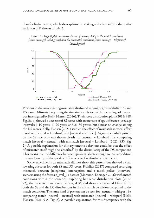
COLLECTION AND ANALYSIS OF MULTI-CONDITION AUDIO RECORDINGS 67
than for higher scores, which also explains the striking reduction in EER due to the exclusion of P, shown in Tab. 2.
Figure 2 - Tippett plot: normalised scores [+norm, -CV] in the match condition [voice message] (solid green) and the mismatch condition [voice message – telephone]
(dotted pink)
Previous studies investigating mismatch also found varying degrees of shifts in SS and DS scores. Mismatch regarding the time-interval between the recordings of interest was investigated by Kelly, Hansen (2016). Their score distribution plots (2016: 418, Fig. 3a, b) showed a decrease of SS scores with an increase of age difference (used age intervals: 1-10 years, 11-20 years, and 21-30 years), but almost no change among the DS scores. Kelly, Hansen (2021) studied the effect of mismatch in vocal effort based on [neutral – Lombard] and [neutral – whisper]. Again, a left-shift pattern on the SS side only was shown clearly for [neutral – Lombard], i.e. comparing match [neutral – neutral] with mismatch [neutral – Lombard] (2021: 935, Fig. 2). A possible explanation for this asymmetric behaviour could be that the effect of mismatch itself might be ‘absorbed’ by the dissimilarity of the DS component. This means that the difference between speakers is large enough so that a condition mismatch on top of the speaker differences is of no further consequence.
Some experiments on mismatch did not show this pattern but showed a clear lowering of scores for both SS and DS scores. Fröhlich (2017) compared recording mismatch between [telephone] interception and a mock police [interview] scenario using the forensic_eval_01 dataset (Morrison, Enzinger, 2016) with match conditions within the scenarios. Exploring her score distribution plots (2017: 72), the presented raw scores [-norm, -CV] did show a substantial left-shift for both the SS and the DS distributions in the mismatch condition compared to the match condition. The same kind of pattern can be seen for [neutral – whisper], i.e. comparing match [neutral – neutral] with mismatch [neutral – whisper] (Kelly, Hansen, 2021: 935, Fig. 2). A possible explanation for this discrepancy with the

68 KATHARINA KLUG, MICHAEL JESSEN, YOSEF A. SOLEWICZ, ISOLDE WAGNER
asymmetric pattern shown above could be as follows. When the channel conditions are strong and systematic (as in forensic_eval_01) they might – simply spoken – act as a “noise-vector” that is almost uncorrelated with the “speaker-vector”. For that reason, the channel influence and the (different-)speaker influence are additive. In a broader sense, [whisper] might also be conceived of as a channel effect. Like a noisy channel, it is corrupting parts of regular speech. This mode of corruption might be fairly independent of the speaker differences, and again, creating an additive effect in reducing DS scores. In contrast to this pattern, the difference between [telephone] and [voice message] investigated here does not seem to be strong, systematic, and independent enough to have a clear effect on DS scores.
Figure 3 - Tippett plot: normalised and calibrated scores using cross validation calibration [+norm, +CV] in the match condition [voice message] (solid green)
and the mismatch condition [voice message – telephone] (dotted pink)
Fig. 3 is based on normalised scores followed by cross validation calibration using Bio-Metrics [+norm, +CV]. One expected effect of calibration that can be seen in the Tippett plot is that the intersection between the SS and DS distribution is located very closely at LLR = 0. Moreover, it can be observed that there is a shift towards the centre of the plot for both mismatch distributions (SS and DS). This behaviour has the effect that the values from the mismatch condition (now fully calibrated LLRs) fall entirely within the range of values from the match condition (a similar pattern can also be found in the age mismatch study by Kelly, Hansen, 2016: 2418, Figs. 3c, d). This means that under mismatch conditions it is not possible to obtain the same range of LLRs as under match conditions. Furthermore, it can be seen that the intersection point is higher on the y-axis under mismatch than match, i.e. the EER is higher.

COLLECTION AND ANALYSIS OF MULTI-CONDITION AUDIO RECORDINGS 69
Figure 4 - Tippett plot: normalisation effect [+norm, +CV] (solid lines) in comparison to raw scores [-norm, +CV] (dotted lines) in the match condition [voice message] (green)
and the mismatch condition [voice message – telephone] (pink)
Fig. 4 shows the effect of normalisation, hence the improvement of the system’s performance, on both match (green) and mismatch condition (pink). In comparison with the non-normalised raw scores (dotted lines) [-norm, +CV], the normalised distributions (solid lines) [+norm, +CV] are stretched across a wider range. This effect is stronger in the match condition (green), as the normalised scores are constantly higher for the SS and constantly lower for the DS distribution. For mismatch, the pattern is less clear especially in ranges lower than -6.4, where normalised and non-normalised results cross.
Table 2 - Summary of EER and Cllr results for match and mismatch conditions under different system options
Condition System options EER in % Cllr EER in %w/o speaker P
Cllrw/o speaker P
match
[-norm, -CV] 4.3 2.37 - -[-norm, +CV] 4.4 0.18 - -[+norm, -CV] 2.1 0.62 - -[+norm, +CV] 2.2 0.12 - -
mismatch
[-norm, -CV] 16.3 14.73 7.9 7.7[-norm, +CV] 17.7 0.84 10.9 0.43[+norm, -CV] 12.1 0.66 9.0 0.70[+norm, +CV] 14.9 0.54 11.3 0.41
Tab. 2 shows EERs and Cllrs for all performed tests. Within both match and mismatch condition, normalisation [+norm, -CV] has the effect of improving discrimination (lowered EER) compared to the raw scores [-norm, -CV]. This

70 KATHARINA KLUG, MICHAEL JESSEN, YOSEF A. SOLEWICZ, ISOLDE WAGNER
is in line with expectation. An exception is the mismatch test in which speaker P is excluded; in this case, after normalisation, the EER is slightly higher instead of lower. Normalisation also has a certain calibration effect, i.e. unacceptably high Cllr values among raw scores are lowered to more acceptable values (smaller than 1) after normalisation. Only after applying calibration [+CV] the Cllr values are at their lowest. With sufficiently large calibration sets (the VOCALISE manual recommends at least 15 speakers with two recordings per speaker, but preferably more speakers) calibration should have a negligible effect on discrimination, i.e. EER before and after calibration should be approximately the same. This is true for the results of the match condition, but there are exceptions for the results of the mismatch condition. In the mismatch condition, the minimum recommendation for the use of calibration could not be met, which probably leads to the exceptional patterns. It is also possible that for calibration sets below the recommended minimum, the effect of calibration may be less effective because the calibration parameters may be influenced by the specific individual speaker patterns in the calibration set, rather than just reflecting the case conditions. Hence, Cllr may now be higher than if the recommendations were met.
Comparing the results of the mismatch condition with and without speaker P, it can be observed that the exclusion of this speaker causes a substantial improvement in discrimination, i.e. a reduction in the EER. Cllr is also substantially improved for the raw scores, but for the normalised scores the effects are small, or Cllr even deteriorates [+norm, -CV].
After having shown the results for mismatch compared to match, the following Tippett plots compare the unfamiliar match condition [voice message] with the more established match condition [telephone] interception. Figs. 5 and 6 compare two tests with match conditions, namely [voice message – voice message] shown earlier (represented in solid green) with [telephone – telephone] (represented in dashed blue). The [telephone] test is based on the corpus GFS 2.0 (Solewicz et al., 2017). Fig. 5 shows the results for raw scores [-norm, -CV], Fig. 6 for normalised scores (without applying calibration) [+norm, -CV].
Fig. 5 shows that on the level of raw scores there is a shift towards higher values from the condition [telephone – telephone] to [voice message – voice message]. That shift applies to both SS and DS comparison results to about the same extent. Given the complexity of an x-vector system, it is difficult to explain this shift. It is possible that [voice message] data are only scarcely represented in the training data of the system, whereas [telephone] conversation data are represented abundantly. As a result, it is possible that above-average similarities are found between [voice message – voice message] comparisons, resulting in higher scores. It could also be relevant that [voice message] data contains spectral information up to 7 kHz, while [telephone] data is much more limited. Accordingly, the entire 4 kHz range can be explored in [voice message] data after down sampling, which might lead to a higher score. Finally, the trends of quality degradation in the tested [voice message]

COLLECTION AND ANALYSIS OF MULTI-CONDITION AUDIO RECORDINGS 71
data mentioned in § 5.1 (especially in-vehicle noise) might have led to a similarity pattern that is not present in the [telephone] data.
Figure 5 - Tippett plot: raw scores [-norm, -CV] in the match condition [voice message – voice message] (solid green) and the match condition [telephone – telephone]
(dashed blue)
Figure 6 - Tippett plot: normalised scores [+norm, -CV] in the match condition [voice message – voice message] (solid green) and the match condition [telephone – telephone]
(dashed blue)
Fig. 6 shows that when normalisation is applied, the difference between the two match conditions [voice message] and [telephone] is reduced. On the DS side, the difference has almost disappeared. On the SS side, the difference is limited to only some areas of the cumulative distribution. As explained earlier, normalisation
72 KATHARINA KLUG, MICHAEL JESSEN, YOSEF A. SOLEWICZ, ISOLDE WAGNER
is performed by feeding additional data into the system that corresponds to the conditions of the case. In comparisons within [voice message] data this normalisation set consists of [voice message] data, in the case of [telephone]-based comparisons, the normalisation set consists of [telephone] recordings. Providing case-relevant normalisation data seems to reduce quite strongly the differences of the score distributions that are found when no normalisation is applied, leading to a large degree of overlap between the two score distributions. About the same amount of overlap is found if cross validation calibration is applied to the normalised scores [+norm, +CV] separately for each condition (not shown here).
When looking at the similarity of the distributions in Fig. 6, one may wonder why there is such a clear mismatch effect at all. In other words, when a test based on [voice message] data leads to very similar score distributions as a test based on [telephone] interception, why is performance degraded in comparisons where the questioned speaker’s recording is a [voice message] while the suspected speaker’s recording is a [telephone] intercept? For an explanation one should probably consider the raw values, not the normalised scores. The raw scores are the values directly resulting from the automatic processing that takes place in the multidimensional space of the acoustic features and their models. If, as assumed above, the condition [voice message] was poorly represented in the training data of the system, these recordings might have stuck out in the multidimensional space, making them not only similar to other [voice message] recordings (as assumed above), but also dissimilar to recordings in other conditions, such as [telephone] recordings. Hence the score reductions under mismatch. The above-mentioned degradation in quality of [voice message] data compared to [telephone] data may have increased this effect.
8. ConclusionsThe goal of the presented FORBIS project was to compile a real case forensic corpus to validate the performance of FASR under forensically realistic conditions and subsequently apply it to a greater extent in speaker comparison casework. Here, the match condition [voice message] as well as the mismatch condition [voice message – telephone] were validated. Results from the match condition [voice message] were compared to the match condition [telephone], a condition which has been far more extensively studied in casework application as well as in research projects.
When examining the results in § 7 with regard to their impact on forensic casework, the following aspects can be emphasized.
Comparison of the match condition [voice message – voice message] with the mismatch condition [voice message – telephone] has shown that when the raw scores or the normalised scores are examined, there is a reduction of SS scores from the match to the mismatch condition and essentially no change between the DS scores. As a result, the distributions overlap more under the mismatch than the match condition and speaker discrimination is lower under the mismatch than

COLLECTION AND ANALYSIS OF MULTI-CONDITION AUDIO RECORDINGS 73
under the match condition. Left-shift among SS but not DS scores is a pattern that has been found elsewhere in the literature and a possible explanation has been given above. In casework, calibration would normally be applied, that means the forensically most relevant patterns are the ones illustrated in Figs. 3 and 4. These indicate that the system is more powerful under the match condition than under the mismatch condition, i.e. EER and Cllr are lower and there is a wider range of possible LLRs in the match condition. Casework can be conducted under both conditions if validation tests are available. Although speaker discrimination abilities are lower under mismatch, the system is still forensically useful, i.e. mismatch is not an exclusion criterion.
The results for the mismatch condition improved when Zoo plots were applied and the one speaker classified as “phantom” was removed from analysis. This improvement seems to indicate that screening for outlier speakers using Zoo plots can improve speaker discrimination and calibration.
The comparison of the unfamiliar condition [voice message] with the established condition [telephone], both in match condition, shows that both have similarly high speaker discrimination power (voice message: EER = 2.2%, telephone: EER = 2.3%). This means that if validation is available (as shown here), automatic speaker recognition can be performed equally well in comparisons based on [voice message] data as in comparisons based on [telephone] interception. It is not the case that [voice message] is a condition that is particularly challenging in itself. That would distinguish it from challenging conditions such as [Lombard] speech or [whisper] addressed in Kelly, Hansen (2021), where match condition performance within this [challenging] condition is lower than within a [neutral] condition, although mismatch between [neutral] and [challenging] conditions would be even poorer.
What if there was no validation data – could [voice message] cases be carried out with validation data based on [telephone] speech? Based on what we know from the presented tests, there is a difference in the score distributions of the conditions [voice message] and [telephone]. The difference is clear when looking at the raw scores but is much smaller when applying normalisation with case-relevant data to both, [voice message] and [telephone] data, respectively. If, for example, [voice message] comparisons are calibrated with [telephone] data, there will be a shift in LLRs that basically corresponds to the difference in the scores shown in Fig. 5 (when calibration is based on the raw scores [-norm, +CV]) or the scores shown in Fig. 6 (when calibration is based on the normalised scores [+norm, +CV]). A correct interpretation of the speaker comparison result would be hindered by the unknown extent of the shift. The hindrance would be low if normalisation was possible, i.e. if [voice message] data could be provided, but higher if not. It is a matter of judgement to define what constitutes a sufficiently small or too large interpretability bias. What should be done is to perform more tests under further unfamiliar conditions to get an impression about what constitutes large or small differences in the score distributions and whether results for some unfamiliar conditions could be interpolated based on previous tests. It is possible, for example,

74 KATHARINA KLUG, MICHAEL JESSEN, YOSEF A. SOLEWICZ, ISOLDE WAGNER
that audio data from outdoor video recordings lead to larger score shifts than the ones observed here.
More data must be collected. Data collection should be done continuously by adding relevant casework data to the already existing corpus. This would allow for testing of additional languages (e.g. Turkish, Russian), recording conditions (e.g. video, interior surveillance) as well as mismatch scenarios for FASR application. Initial validation tests for language mismatch [Arabic – German] under [telephone] condition have already been carried out. However, more data is needed for valid and reliable interpretations. In addition, further languages and recording conditions in casework could become more frequent as new criminal networks emerge and technical possibilities develop.
AcknowledgementsThe authors would like to thank Justin Hofenbitzer and Kjartan Beier for their contribution to the segmentation and anonymisation work as well as Linda Gerlach for discussing results gained from pre-tests and Finnian Kelly for providing important leads on Zoo plot screening and the interpretation of the results. We are grateful for the comments and suggestions gained from our colleague Almut Braun and from three anonymous reviewers to a previous version of this paper. In addition, we value each real forensic audio and video recording provided by colleagues from other departments within the BKA. Organisational support was also provided by the German-Israeli Cooperation on Counter-Terrorism Technology. This work was financially supported by the EU Internal Security Fund [grant number IZ25-5793-2018-34].
Bibliography
Bio-metrics 1.8 (2019). Performance Metrics Software, Oxford Wave Research Ltd., https://oxfordwaveresearch.com/products/bio-metrics/.Boersma, P., Weenink, D. (2016). Praat: doing phonetics by computer. [Computer program] Version 6.0.17, retrieved 21 April 2016 from http://www.praat.org/.Drygajlo, A., Jessen, M., Gfroerer, S., Wagner, I., Vermeulen, J. & Niemi, T. (2015). Methodological guidelines for best practice in forensic semiautomatic and automatic speaker recognition. Frankfurt: Verlag für Polizeiwissenschaft. https://enfsi.eu/wp-content/uploads/2016/09/guidelines_fasr_and_fsasr_0.pdf/ Accessed 05.12.2021.Dunstone, T., Yager, T. (2009). Biometric system and data analysis. New York: Springer.Fröhlich, A. (2017). Evaluation des forensischen Sprechererkennungssystems iVocalise anhand eines Zwillingsdatensets und eines Datensets, welches forensische Echtfallszenarien abbildet. Master thesis, Universität Zürich.

COLLECTION AND ANALYSIS OF MULTI-CONDITION AUDIO RECORDINGS 75
Gold, E., French, P. (2019). International practices in forensic speaker comparisons: second survey. In International Journal of Speech Language and the Law, 26, 1-20. http://dx.doi.org/10.1558/ijsll.38028Hansen, J.H.L., Boril, H. (2018). On the issues of intra-speaker variability and realism in speech, speaker, and language recognition tasks. In Speech Communication, 101, 94-108. https://doi.org/10.1016/j.specom.2018.05.004Jessen, M. (2018). Forensic voice comparison. In Visconti, J. (Ed. in collab. with Rathert, M.). Handbook of communication in the legal sphere. Berlin: Mouton de Gruyter, 219-255.Kelly, F., Hansen, J.H.L. (2016). Score-aging calibration for speaker verification. In IEEE/ACM Transactions on Audio, Speech, and Language Processing, 24(12), 2414-2424. https://doi.org/10.1109/TASLP.2016.2602542Kelly, F., Forth, O., Kent, S., Gerlach, L. & Alexander, A. (2019a). Deep neural network based forensic automatic speaker recognition in VOCALISE using x-vectors. Proceedings of the Audio Engineering Society (AES) Conference Audio Forensics, Porto, Portugal, 18-20 June 2019, 1-7. https://www.aes.org/e-lib/online/search.cfm/ Accessed 05.12.2021.Kelly, F., Fröhlich, A., Dellwo, V., Forth, O., Kent, S. & Alexander, A. (2019b). Evaluation of VOCALISE under conditions reflecting those of a real forensic voice comparison case (forensic_eval_01). In Speech Communication, 112, 30-36. http://dx.doi.org/10.1016/j.specom.2019.06.005Kelly, F., Hansen, J. (2021). Analysis and calibration of lombard effect and whisper for speaker recognition. In IEEE/ACM Transactions on Audio, Speech, and Language Processing, 29, 927-942. https://doi.org/10.1109/TASLP.2021.3053388Künzel, H.J. (2013). Automatic speaker recognition with crosslanguage speech material. In The International Journal of Speech, Language and the Law, 20(1), 21-44. http://dx.doi.org/10.1558/ijsll.v20i1.21Morrison, G.S. (2011). A comparison of procedures for the calculation of forensic likelihood ratios from acoustic-phonetic data: Multivariate kernel density (MVKD) versus Gaussian mixture model – universal background model (GMM-UBM). In Speech Communication, 53, 242-256. https://doi.org/10.1016/j.specom.2010.09.005Morrison, G.S. (2013). Tutorial on logistic-regression calibration and fusion: converting a score to a likelihood ratio. In Australian Journal of Forensic Sciences, 45, 173-197. https://doi.org/10.1080/00450618.2012.733025Morrison, G.S., Enzinger, E. (2016). Multi-laboratory evaluation of forensic voice comparison systems under conditions reflecting those of a real forensic case (forensic_eval_01) –introduction. In Speech Communication, 85, 119-126. http://dx.doi.org/10.1016/j.specom.2016.07.006Morrison, G.S., Kelly, F. (2019). A statistical procedure to adjust for time-interval mismatch in forensic voice comparison. In Speech Communication, 112, 15-21. https://doi.org/10.1016/j.specom.2019.07.001Morrison, G.S., Enzinger, E., Hughes, V., Jessen, M., Meuwly, D., Neumann, C., Planting, S., Thompson, W.C., Van der Vloed, D., Ypma, R.J.F., Zhang, C.,

76 KATHARINA KLUG, MICHAEL JESSEN, YOSEF A. SOLEWICZ, ISOLDE WAGNER
Anonymous, A. & Anonymous, B. (2021). Consensus on validation of forensic voice comparison. In Science and Justice, 61, 229-309. https://doi.org/10.1016/j.scijus.2021.02.002Nash, J. (2019). The effect of acoustic variability on automatic speaker recognition systems. PhD dissertation, University of York.Rose, P. (2002). Forensic speaker identification. London: Taylor & Francis.Shum, S., Dehak, N., Dehak, R. & Glass, J.R. (2010). Unsupervised speaker adaptation based on the cosine similarity for text-independent speaker verification. Proceedings of Odyssey, Brno, Czech Republic, 28 June-1 July 2010, 76-82.Solewicz, Y.A., Jessen, M. & van der Vloed, D. (2017). Null-hypothesis LLR: A proposal for forensic automatic speaker recognition. Proceedings of Interspeech, Stockholm, Sweden, 20-24 August 2017, 2849-2853.Van Leeuwen, D.A., Brümmer, N. (2007). An introduction to application-independent evaluation of speaker recognition systems. In Müller, C. (Ed.). Speaker classification I: Fundamentals, features, and methods. Berlin: Springer, 330-353.Van der Vloed, D., Kelly, F. & Alexander, A. (2020). Exploring the effects of device variability on forensic speaker comparison using VOCALISE and NFI-FRIDA: A forensically realistic database. Proceedings of Odyssey, Tokyo, Japan, 1-5 November 2020, 402-407. http://dx.doi.org/10.21437/Odyssey.2020-57Vocalise 2.7 (2019). Automatic Speaker Recognition Software, Oxford Wave Research Ltd., https://oxfordwaveresearch.com/products/vocalise.

DOI: 10.17469/O2108AISV000004
JUSTIN J.H. LO
Seeing the trees in the forest: Diagnosing individual performance with acoustic data in likelihood ratio based forensic voice comparison
System testing is a crucial part of likelihood ratio based forensic voice comparison, but the evaluation of system performance has thus far focused on global metrics, with little attention paid to the variation in individual performance and the factors behind such variation. Using long-term formant distributions as a case study, this study applies the notion of biometric menagerie to analyse performance on the individual level, and further explores the connection between performance and the underlying acoustic data. Zooplot analysis reveals distinct distributions of how individual speakers perform for each long-term formant. Acoustic analysis further reveals clear patterns in the formant data displayed by speakers with outlying performance. Together, the findings support the view that individual-level analysis can offer useful diagnostic insights into system performance that are unavailable in global-level assessment.
Keywords: forensic voice comparison, long-term formant distributions, likelihood ratios, individual performance, zooplots.
1. IntroductionIn cases of forensic voice comparison (FVC), a voice sample from a speaker whose identity is unknown is typically compared with another sample from a known speaker. To this end, features in the voice and speech are analysed to assess both the similarity between the questioned and known samples, and the typicality of the features observed. In recent years, the adoption of likelihood ratios (LRs) in forensic speech science offers an explicit framework to assess voice evidence with respect to two competing hypotheses: (1) that the two speakers are the same, and (2) that the unknown speaker is not the known speaker, but another person in the relevant population. Within this framework, the analyst’s conclusions are expressed in the form of a verbal or numerical LR to indicate the direction and degree of support offered by the evidence for one of the propositions. As LRs are sensitive to not only the speech features chosen, but also the method and the database of speakers used in their derivation, these must be tested to ensure that the resultant systems are valid and reliable.
In numerical LR-based FVC, system evaluation is predominantly conducted on the global level, where the strength of performance is indicated by means of a single metric score. The most commonly used metrics are the equal error rate (EER) and

78 JUSTIN J.H. LO
the log likelihood ratio cost function (Cllr, Brümmer, du Preez, 2006). The EER identifies the percentage of comparisons with contrary-to-fact outcomes, at a score threshold where the rate of misses (same speaker identified as different) is equal to the rate of false matches (different speakers identified as the same). Cllr, on the other hand, takes into account the magnitude of errors, such that contrary-to-fact LRs of a larger magnitude incur higher penalty and, in turn, higher Cllr. A Cllr that is greater than 1 indicates that the system is poorly calibrated. For both of these metrics, stronger system performance is indicated by smaller values: The closer they are to 0, the better the system is judged to be performing.
Other graphical means of evaluation, such as receiver operating characteristic (ROC) curves, detection error tradeoff (DET) curves and Tippett plots, are also often employed to provide more information about the overall performance of the system (see Morrison, Enzinger, 2016). Commonly used in the assessment of automatic speaker recognition (ASR) systems, ROC curves plot the rate of true matches against the rate of false matches across a range of acceptance thresholds in a single curve, while DET track the rate of false matches against the rate of misses in a similar fashion. Meanwhile, Tippett plots trace performance of same-speaker and different-speaker comparisons in separate curves to visualise the cumulative distribution of scores (or LRs) in each type of comparison.
As much as the above metrics and graphs can illustrate the global level of system performance, their diagnostic value can be limited. A more microscopic view of system performance, beyond rates and sizes of error, can be obtained by examining the performance of individual speakers. By analysing in detail the speakers who perform exceptionally well or disproportionately contribute to errors, researchers can gain insights into the nature of the errors in the system and work towards improving system design in a targeted manner. Further, identifying individual voices who are difficult to match against any speakers in the same database may be helpful for optimising homogeneity within forensic databases (San Segundo, Tsanas & Gómez-Vilda, 2017).
To date, analysis of individual performance remains rarely performed in the context of FVC, and the causes behind speakers being identified as outliers within any tested system are still underexplored. In addition to technical properties of the audio samples, such as non-uniform duration and acoustic quality (Nash, 2019), variation of individual performance in any given system can arise due to physiological and behavioural reasons, as well as the impact of these factors on the quality of data capture (Dunstone, Yager, 2009). Fundamental frequency, for example, is susceptible to variation due to physiological factors in both the short and the long term (Braun, 1985; Rhodes, 2012). In terms of behaviour, speakers may seek to disguise their voice. They may also shout at such a volume that causes clipping in the recording, thus impacting data capture. A close analysis of LRs from individual speakers and the corresponding speech data used to generate those LRs may thus not only be useful in diagnosing the sources of variation in individual

SEEING THE TREES IN THE FOREST 79
performance, but also more generally help understand the relationship between input and output in numerical LR-based testing.
Within the context of ASR, Alexander, Forth, Nash & Yager (2014) has proposed preliminary links between individual performance and aspects of voice quality. However, subjective judgments of voice quality are far removed from cepstral coefficients, the acoustic features used in ASR systems that are highly abstract, and do not encode the same speaker-specific information (French, Foulkes, Harrison, Hughes, San Segundo & Stevens, 2015). The connection between individual LR performance and the input data thus warrants further investigation.
To address this issue, the present study seeks to extend the analysis of individual LR performance to systems based on linguistic-phonetic variables, using long-term formant distributions (LTFDs) as a case study. It additionally explores the connection between individual performance as derived from LRs and the underlying speech data. Following previous analyses of individual performance, this study makes use of the notion of “biometric menagerie” (see below §3) to classify speakers who perform exceptionally well or poorly. Individual LTF data from these outlying speakers are considered with respect to others in the population to analyse any links with their performance.
2. Long-term formant distributionsThe use of LTFDs as viable speaker discriminants in FVC is first proposed in Nolan, Grigoras (2005). Instead of individual sounds, LTFDs measure the whole collection of formant estimates from all vowels (or voiced sounds) present in the recording. LTFDs are thus argued to capture the overall filtering behaviour of the supralaryngeal vocal tract, reflecting not only its physiology but also the speaker’s idiosyncratic articulatory habits. There is empirical evidence in support of the latter, as LTF1 and LTF2 means have respectively been found to correlate with the vocal settings of raised/lowered larynx and fronted tongue body (French et al., 2015). Further support for the inclusion of LTFDs in the FVC toolkit can be found in their independence from other acoustic and temporal measures, such as fundamental frequency and speaking rate (Moos, 2010).
Speaker-specific information in LTFDs lies not only in the location of the peaks or means of the distributions, but also in their overall shapes (Cho, Munro, 2017). Studies conducted within the LR framework have tested the discriminatory potential of LTFDs in English and German and reported low error rates in both languages (Becker, Jessen & Grigoras, 2008; French et al., 2015; Gold, French & Harrison, 2013). LTFs of higher formants have been found to provide stronger performance than those of lower formants (Gold et al., 2013), while using multiple formants in combination can further improve performance (Becker et al., 2008; Gold et al., 2013).
As semi-automatic formant-based acoustic features, LTFDs are readily interpretable in linguistic-phonetic terms, as opposed to cepstrum-based features used in automatic approaches, which do not display any comparable degree of interpretability (Rose,

80 JUSTIN J.H. LO
2003). This characteristic is considered to make LTFDs a useful set of features for the present exercise. Previous attempts at individual analysis for LTFDs have also sought to explore their links with individual LR performance, such as in Hughes, Harrison, Foulkes, French, Kavanagh & San Segundo (2018), who found considerably variable behaviour across individual speakers, not only in the strength of evidence produced, but also in the stability of their performance in face of channel variation. Importantly, in systems that combined LTF1-3, their corresponding bandwidths and delta coefficients as input, none of LTF1-3 means was found to be able to predict an individual’s performance, although it must be noted that only the relationship between performance and means was considered but not that between performance and the speakers’ full distributions.
3. The biometric menagerieThe current study makes use of zooplots, a diagnostic tool used in the field of biometrics to visualise individual user performance. The zooplot is built upon the idea of a “biometric menagerie”, developed by Doddington, Liggett, Martin, Przybocki & Reynolds (1998) and later expanded on by Dunstone, Yager (2009), where speakers are classified into user groups or animals based on their individual performance. In a zooplot, each speaker’s performance in same-speaker comparisons (or genuine performance) is plotted against their performance in different-speaker comparisons (or imposter performance). The use of zooplots thus facilitates the identification of problematic speakers in the database for further analysis and diagnosis. Additionally, the distribution of speakers in a zooplot can be indicative of systematic weaknesses in the algorithm or the database used. A predominance of speakers who perform well in different-speaker comparisons but poorly in same-speaker comparisons, for example, may be an outcome of poor-quality enrolment in the database (Dunstone, Yager, 2009).
In their original formulation, Doddington et al. (1998) distinguishes a default group of speakers, sheep, from other speakers who tend to contribute disproportionately to system errors. These animal groups include goats, whose voices are particularly difficult to match and hence likely produce errors in same-speaker comparisons; lambs, who may disproportionately account for false matches due to their voices being easily imitable; and wolves, whose voices may easily imitate others’ and thus also contribute to false matches. Dunstone, Yager (2009) introduces a set of relational animals, which are defined by the relationship between a speaker’s performance in same-speaker comparisons and in different-speaker comparisons, rather than their performance in a single type of comparisons. Described in FVC terms, these groups include:– doves, who perform relatively well in both types of comparisons;– worms, who perform relatively poorly in both types of comparisons;– phantoms, whose voice characteristics are difficult to match against any speaker
and so who perform well in different-speaker comparisons but poorly in same-speaker comparisons; and

SEEING THE TREES IN THE FOREST 81
– chameleons, who can be easily matched with (or camouflage as) any speaker and thus perform well in same-speaker comparisons but not in different-speaker comparisons.
This study focuses on the relational groups introduced by Dunstone, Yager (2009), as they allow specific speakers who belong to each of these groups to be identified. Members of each group can then be further analysed for the causes behind their outlying performance within the tested system to be potentially diagnosed.
4. Methodology4.1 Materials
In the present study, a subset of high-quality microphone recordings from the Voice ID Database (Royal Canadian Mounted Police, 2010-2016) were used, consisting of 60 adult male bilingual speakers of Canadian English and French (mean age = 27.7 years), all of whom recorded the same sets of read materials in both languages. Metadata on speakers’ language and social background were limited, and speakers were selected on the basis that they participated in recording for both languages and did not self-report knowledge of any other languages. 23 and 31 speakers reported their first language to be English and French respectively (mean age of first exposure to second language = 5.3 years), while the remainder reported to be simultaneously bilingual in both. The current analysis is limited to the data from English.
All speakers were recorded reading 20 phonetically balanced sentences extracted from the Harvard sentences. 22 speakers were also recorded reading an abridged version of The Rainbow Passage (Fairbanks, 1960). All recordings were first orthographically transcribed in Praat (Boersma, Weenink, 2016), where hesitations, repetitions, mispronunciations and deviations from the set material were retained as far as possible, although partial words were ignored. Automatic segmentation was performed using the Montreal Forced Aligner (McAuliffe, Socolof, Mihuc, Wagner & Sonderegger, 2017), which was then manually checked for errors in alignment and corrected where necessary.
While the quality of the recordings may result in validity measures that are more optimistic than those obtained from forensically realistic materials, the controlled nature of the materials has the advantage of ensuring that variation in LTFDs can be attributed to speaker physiology and behaviour, rather than differences in speech content.
4.2 Data extraction
Formant centre frequency estimates for the first four formants were extracted in Praat at 10 ms intervals from the onset to the offset of all vowels and glides. Formant extraction was automated with a Praat script, using the Burg algorithm for linear predictive coding, with the formant tracker set to search for 6 formants up to a maximum formant frequency of 5500 Hz in 25 ms frames. These settings were determined by preliminary testing to be the most appropriate for the current set

82 JUSTIN J.H. LO
of speakers and remained fixed for all speakers. Each speaker’s recording contains 26.2 s of pure vowels and glides on average, yielding a grand total of 172,054 sets of formant estimates from all speakers for system testing.
4.3 Performance testing
Five systems, each using a different set of input parameters, were tested in total. In addition to the combination of all four LTFs, each LTF was tested individually to facilitate one-to-one comparison with the acoustic data.
To test each system, the 60 speakers were randomly divided into test, training and background sets, each made up of 20 speakers. The computation of LRs followed the two-stage process set out in Morrison (2013). In the feature-to-score stage, comparisons were conducted for all speaker-pairs in the test set, with each speaker acting in turn as the questioned and known speaker for all speakers, resulting in 20 same-speaker and 380 different-speaker comparisons. LTFDs were modelled and compared using the Gaussian mixed model-Universal background model (GMM-UBM) approach (Becker et al., 2008; Reynolds, Quatieri & Dunn, 2000), implemented by means of the mclust package in R (R Core Team, 2018; Scrucca, Fop, Murphy & Raftery, 2016). As only a single recording was available from each speaker, the first half of the recording was taken to form the known sample for the speaker, and the second half was taken to form the questioned sample. The reference population was modelled with a UBM, a single GMM composed of 12 Gaussians calculated using data pooled together from all 20 speakers in the background set. In each comparison, a GMM for the known speaker was derived by using data from the known sample to adapt the UBM by means of maximum a posteriori estimation, and the output score of the comparison was calculated by Equation (1). In the score-to-LR stage, the test scores were then calibrated with output scores similarly computed from the training set to obtain log10LRs (LLRs) in a logistic regression procedure. LLR > 0 in a comparison indicates support for the same-speaker hypothesis, while LLR < 0 indicates support for the different-speaker hypothesis. As such, negative LLRs in same-speaker comparisons and positive LLRs in different-speaker comparisons are considered to be contrary-to-fact errors.
(1)
where x1, x2, ..., xN correspond to each set of input data from the questioned sample, S = suspect GMM and B = background UBM.
System validity was then assessed using EER and Cllr. The whole sampling and testing procedure was repeated 100 times, in order to minimise the effect of speaker random sampling on the resultant LRs and validity metrics (Wang, Hughes & Foulkes, 2019), as well as to ensure all speaker-pairs were compared.

SEEING THE TREES IN THE FOREST 83
4.4 Individual-level analysis
To visualise individual LR performance, zooplots for each system were constructed by plotting each speaker’s average performance in different-speaker comparisons against their performance in same-speaker comparisons, where speakers with stronger performance were positioned towards the top and the right of the plot. In this study, average performance of any speaker is defined as the arithmetic mean of LLRs from all same- or different-speaker comparisons across 100 repetitions involving that speaker.
Individual-level analysis of LR performance was conducted in three ways. First, the overall distribution of speakers on the zooplots was analysed, in terms of both the absolute values of LLRs (as they can be directly interpreted) and the relative positions of speakers. Second, speakers with outlying performance in each system were identified and categorised into one of the four relational animal groups defined in §3. Following Dunstone, Yager (2009), doves are defined as speakers whose average performance is within the best 25% of all speakers in both types of comparisons. This group can therefore be located in the top right corner of the zooplot, as they comprise speakers with the highest, most positive mean LLR in same-speaker comparisons (SS-LLR) and the lowest, most negative mean LLR in different-speaker comparisons (DS-LLR). Worms, phantoms and chameleons are analogously defined, as outlined in Tab. 1. Speakers whose average mean LLR lies between the top (or bottom) 25% to 30% were additionally identified as near-members of animal groups to mitigate cliff-edge effects of borderline cases documented in O’Connor, Elliott, Sutton & Dyrenfurth (2015). Membership of relational groups was then analysed in each system and compared across different systems. Third, to explore the relationship between LR performance and acoustic data, LTFDs of speakers classified as (near-)members of relational groups were compared with those of the other speakers.
Table 1 - Inclusion criteria for doves, worms, phantoms and chameleons and their locations in zooplots
Mean same-speaker LLR
Mean different-speaker LLR Location
Doves Highest 25% Lowest 25% Top rightWorms Lowest 25% Highest 25% Bottom left
Phantoms Lowest 25% Lowest 25% Top leftChameleons Highest 25% Highest 25% Bottom right
5. Results5.1 Global metrics
Performance for each system, measured in Cllr and EER, is illustrated in Fig. 1. Mean Cllr for all systems (and indeed all repetitions) was below 1, indicating that

84 JUSTIN J.H. LO
the systems were well calibrated. The system combining all four LTFs reported the lowest mean Cllr and EER at 0.31 and 7.3%, clearly outperforming systems using only single LTFs. Individually, each of LTF1-4 performed at similar levels, with a mean Cllr between 0.6 and 0.7 and a mean EER of around 20%. Nevertheless, out of all systems using individual LTFs, Fig.1 demonstrates a trend of LTF2 performing the worst, with the highest mean Cllr (0.69) and EER (22.1%), while LTF1 had the lowest mean Cllr (0.62) and LTF4 had the lowest mean EER (19.0%).
Figure 1 - Boxplots of Cllr (left) and EER (right) from system testing
5.2 Individual-level analysis
This section presents results on individual LR performance in the tested systems. In each system, the distribution of LLRs is described with the visual aid of a zooplot. The scales of all zooplots are fixed, in order to facilitate direct comparison across different systems. This is accompanied by an analysis of the classification of animal groups in each system and followed by a comparison of group membership across all systems.
5.2.1 LTF1The zooplot shown in Fig. 2 illustrates the individual LR performance of all 60 speakers in the system based on LTF1. As demonstrated in the zooplot, all speakers reported a negative mean DS-LLR. While mean SS-LLR was positive for most speakers, 12 speakers (20%) reported a negative mean SS-LLR, suggesting that they were not well matched with themselves on average. Performance in SS and DS comparisons is strongly correlated (|r| = .74, p < .0001): Speakers with stronger performance in SS comparisons similarly reported stronger performance in DS comparisons. This is further supported by the absence of any phantoms or chameleons, as only members of the other two relational groups (10 doves and five worms) were identified. Overall, the system produced a narrow range of mean LLRs, with SS-LLR between -0.40 and 2.55, and DS-LLR between -0.48 and

SEEING THE TREES IN THE FOREST 85
-1.47. Most speakers could be found in a dense cluster near the lower left corner of the zooplot.
Figure 2 - Zooplot for system with LTF1 as input (abscissa and ordinate respectively show mean SS-LLR and DS-LLR in log10LR; solid line segments represent 25th
and 75th percentiles; dotted lines indicate mean LLR = 0; members and near-members of relational groups respectively in black and grey)
5.2.2 LTF2As shown in the zooplot in Fig. 3, all speakers also reported a negative mean DS-LLR in the LTF2 system, and a majority of speakers reported a positive mean SS-LLR. Although there were the same number of speakers with negative mean SS-LLR (12) as in the case of LTF1, the magnitude of these negative SS-LLRs was slightly higher (up to -0.80), indicating poorer performance in SS comparisons. Performance in SS and DS comparisons is only moderately correlated (|r| = .51, p < .0001), with a notable presence of speakers in the upper left region of the zooplot, including three speakers who were identified as phantoms. By contrast, only nine doves and three worms were identified for LTF2, fewer than any other individual LTFs.

86 JUSTIN J.H. LO
Figure 3 - Zooplot for system with LTF2 as input
Figure 4 - Zooplot for system with LTF3 as input
5.2.3 LTF3The distribution of speakers in the zooplot for LTF3, as displayed in Fig. 4, shows broad similarities with that for LTF1. No speakers were classified as phantoms or chameleons, and a strong positive correlation was similarly found between mean SS-LLR and DS-LLR (|r| = .92, p < .0001). As in the case of LTF1, a dense cluster of speakers can be located near the lower left corner of the zooplot, including eight worm speakers. Despite the relatively high number of worms, only eight speakers

SEEING THE TREES IN THE FOREST 87
reported a negative mean SS-LLR, none of which exceeded -0.15, indicating smaller contrary-to-fact LLRs on average. Stronger individual performance is also evident among the best-performing doves (12 members and 3 near-members), who are distant from the dense cluster of speakers and are further spread upward and rightward in the zooplot, as a result of more positive mean SS-LLRs and more negative mean DS-LLRs.
5.2.4 LTF4The zooplot for the LTF4 system, as shown in Fig. 5, illustrates a distribution of speakers resembling that for LTF3, although speakers are less clustered towards the lower left corner, indicating an overall greater degree of between-speaker variation in LR performance. Performance between SS and DS comparisons is also strongly correlated (|r| = .87, p < .0001), with particularly high mean SS-LLR (up to 4.78) reported for a number of speakers. At the same time, this system reported the highest number of speakers with outlying performance, where a total of 11 speakers were classified as doves and 13 were classified as worms. The high proportion of outlying speakers suggests that, in the case of LTF4, individual performance is more extremely distributed.
Figure 5 - Zooplot for system with LTF4 as input
5.2.5 All LTFs combinedCompared to the zooplots for individual LTFs, there is evidently a wholesale shift of speakers towards the top of the zooplot in Fig. 6, brought on by more highly negative DS-LLR. Speakers also tend to have much higher SS-LLR, in contrast with zooplots for the other systems, as evidenced by the rightward spread of speakers in Fig. 6. The majority of speakers (42) reported a mean SS-LLR greater than 1, while only three speakers reported marginally negative mean SS-LLR (up

88 JUSTIN J.H. LO
to -0.05). In this system, mean SS-LLR and DS-LLR is moderately correlated (|r| = .59, p < .0001). No phantoms or chameleons were found (although one speaker was classified as near-phantom), while eight doves and six worms were identified. Overall, the distribution of speakers in Fig. 6 is clearly much less clustered than in any of the individual LTF systems.
Figure 6 - Zooplot for system with all four LTFs as input
5.2.6 Speaker classificationFollowing separate analysis within each system above, this section considers the performance of individuals across all LTFD systems. Fig. 7 summarises the animal group classification of all speakers for each system tested. While there are some overlaps between different LTFs, it is clear that each LTF generally captured a different group of outlying speakers. Out of 60 speakers, 21 (35%) were in or near the same group for more than one LTF, but only three speakers (5%) were in or near a relational group for all four LTFs: 441 was consistently classified as a dove; 470 was similarly always in or near the dove group; 119 was classified as a worm for all LTFs except for LTF2, where he was classified as a phantom. The difference between systems is further illustrated by the finding that 12 (20%) speakers were classified as the best-performing doves for one LTF but as the worst-performing worms for another. Across all four LTFs, only five speakers (8%) were not in or near any group, meaning that the vast majority of speakers could be considered an outlying speaker for at least one LTF.

SEEING THE TREES IN THE FOREST 89
Figure 7 - Summary of speakers classified as doves (green), worms (purple), phantoms (blue) or chameleons (orange) in all systems tested (near-members of each group in lighter shade)
In the combined system (top row, Fig. 7), all but two speakers who were in or near an animal group were similarly classified for at least one of the individual LTFs. Out of those 22 speakers, 12 of them shared their classification with the LTF4 system. While systems using other LTFs shared fewer (near-)members of animal groups with the combined system, with LTF2 having only five speakers in common, each of the individual LTFs could uniquely account for at least one classified animal in the combined system. The only exceptions were 217, who was a worm in the combined system but not a member of the outlying groups for any individual LTF, and 113, who was a near-chameleon in the combined system. The latter could be explained by the mixed contribution of his relatively poor DS performance in LTF4, for which he was classified as a worm, and relatively excellent SS performance in LTF3, which resulted in a dove classification.
Overall, the analysis here provides evidence on an individual level that complementary speaker-specific information is available from LTFDs of different formants. As the findings above illustrate, speaker-specific information from each LTFD contributes, albeit in varying degrees, to the classification in the combined system.
5.3 Acoustic analysis
Results of acoustic analysis from the higher formants are first presented here. The full distributions of each speaker’s LTF3 and LTF4, as displayed in Fig. 8, show considerable between-speaker variation in the location of the peak frequency. Peaks in individual LTF3 distributions range from just above 2000 Hz to nearly 2900 Hz, while peaks in LTF4 distributions range from below 3000 Hz to around 3600 Hz. A high degree of variability is similarly found in the shape of the distribution, in terms of both the height and the sharpness of the peaks. Bimodal distributions are also evidenced, albeit rarely, for individual speakers.

90 JUSTIN J.H. LO
Figure 8 - Distributions of LTF3 (left) and LTF4 for all speakers, with doves in green, worms in purple and other speakers in grey (dashed coloured lines indicate near-members
of animal groups; black dashed line indicates group distribution pooled from all 60 speakers)
A close examination of the speakers classified as doves in LTF3 and LTF4 suggests that these are all speakers with relatively extreme peak frequencies, on both the low and high ends of the collection of LTFD. The doves in Fig. 8 show a clear separation from the worms (and near-worms), who are generally close to the group norm, represented by the pooled distribution. The distributions of the worm speakers show peak frequencies that are much further away from the extremes. Their shapes are also relatively unremarkable, with no particularly sharp peaks.
Moving to the lower formants, Fig. 9 shows that LTF1 peaks are limited to a narrow range with relatively little between-speaker variation, which is not surprising in the present context, as F1 is correlated with vowel height and so would be highly constrained when the speech material is uniform across speakers. Nevertheless, the shape of the LTF1 distributions demonstrates substantial variability, especially within the region of frequencies above 500 Hz, where secondary peaks can be found for numerous speakers.
Fig. 9 further shows considerable variability in the distributions of LTF2, especially in the shapes of the distributions. While the peaks for most speakers reside between 1400 and 1600 Hz, the presence of secondary peaks and bimodality is not uncommon among this group of speakers.
As in the cases of LTF3 and LTF4, speakers classified as worms (and to a lesser extent, near-worms) show distributions that strongly resemble the group norms, both in LTF1 and LTF2. Similarly, many dove speakers can be identified as those whose distributions show peaks at especially low or high frequencies within this population. However, it is also clear that the distributions of some doves have peaks at frequencies that are by no means extreme, but indistinguishable from the group average. The distributions of these speakers nonetheless show distinctiveness in other ways, through either particularly sharp peaks (in LTF1 and LTF2) or bimodality (in LTF2). There

SEEING THE TREES IN THE FOREST 91
are also three phantoms and one near-chameleon in the LTF2 system. Due to their low counts, the acoustic correlates of these groups are not analysed in detail, although it can be noted that the three phantoms all appear to demonstrate strong bimodality.
Figure 9 - Distributions of LTF1 (left) and LTF2 for all speakers, with doves in green, worms in purple, phantoms in blue, chameleons in orange and other speakers in grey
(dashed coloured lines indicate near-members of animal groups; black dashed line indicates group distribution pooled from all 60 speakers)
In summary, the acoustic analysis presented in this section demonstrates a clear contrast between doves and worms in their LTFDs. Dove speakers are mostly accounted for by peaks of relatively extreme frequencies. This is most clearly demonstrated in LTF3 and LTF4, but can also be found in the lower formants. While the remaining doves display unremarkable peak frequencies, they show other distinctive characteristics in their distributions. By contrast, the distributions of speakers classified as worms all tend to very similar to the overall distributions of the group, in terms of both peak frequency and shape.
6. DiscussionThe current study set out with two main aims, namely to investigate the effectiveness of individual-level analysis in LR-based FVC, and to explore the relationship between individual LR performance and the underlying data from semi-automatic linguistic-phonetic variables. This section discusses these two themes in turn.
Results from system testing of LTFDs show that, in terms of both Cllr and EER, LTFDs all performed at similar levels when tested individually but reported much stronger system performance when tested in combination. These results corroborate previous findings of higher discriminatory power in formant-based systems using a combination of multiple parameters (Becker et al., 2008; Gold et al., 2013; Hughes, Wood & Foulkes, 2016), as speaker-specific information from each parameter is

92 JUSTIN J.H. LO
modelled in conjunction. Zooplot analysis undertaken in the current study further illustrates the complementarity of speaker specificity from different LTFDs on the individual level, demonstrating how they capture very different groups of speakers with outlying performance.
In the present study, while the worst performance out of all LTFDs was obtained from LTF2, LTF1 reported Cllr and EER that were at least on par with, if not marginally better than, LTF3 and LTF4. Earlier findings that higher formants outperform lower formants in LTFDs (Gold, et al., 2013) are thus not borne out here. Indeed, studies examining the discriminatory potentials of vowel formants have not yielded consistent findings as to whether higher formants convey a greater amount of speaker-discriminatory information than lower formants, which McDougall (2004) argues may depend on the speech materials and conditions. At the same time, when speaker classification is compared across systems, the influence of higher formants appears to dominate in the combined system, as evidenced by the high proportion of classifications shared with LTF3 and LTF4, whereas the contribution of the lower formants is comparatively limited. Zooplots here showed that, in the cases of LTF3 and LTF4, although most speakers had SS-LLRs of low magnitude that were clustered near 0, there were a number of (dove) speakers with exceptional mean LLRs, such that they were distant from the other speakers. LTF1, on the other hand, had no such speakers, and indeed reported a narrow range of mean SS-LLRs and DS-LLRs overall. Thus, it may be the case that the performance of higher formants here was driven by a small number of individuals who performed exceptionally well and thus carried over to the combined system, whereas the performance of LTF1 was driven by the population as a whole.
Beyond classification, the zooplots also allow identification of speakers who contribute most to errors in a system. Among the systems tested, mean SS-LLRs and DS-LLRs are well correlated, but stronger performance is generally found for different-speaker comparisons than for same-speaker comparisons, with a number of speakers reporting negative mean SS-LLRs on average. While other graphical means commonly used to illustrate system performance, such as Tippett plots, can also visualise the difference between the two types of comparison and the proportion of contrary-to-fact LRs, in a zooplot analysis the individuals can be placed into focus for further analysis.
Turning to the relationship between individual performance and the underlying acoustic data, in the case of LTFDs, a close correspondence between distinctive distributions and dove membership was found across all four formants. For many dove speakers, their LTFD peaks lie on the margins of the population distributions, which in turn lead to more skewed LTFDs. This was especially the case in LTF3 and LTF4, where there is considerable between-speaker variability in the location of peaks within this population. Distributions of the remaining dove speakers are distinctive in other ways, such as particularly sharp peaks or bimodality. Worm speakers, on the other hand, had LTFDs characterised by their proximity to the population norms. These findings may in part explain why LTF1-3 means could

SEEING THE TREES IN THE FOREST 93
not predict animal group classification in Hughes et al. (2018), who explored this relationship using linear regression. Within individual LTFDs, speakers with very low or very high means can both be considered atypical, whereas it is speakers with means near the middle – not near the lower end – of the group who are considered highly typical and tend to provide weak evidence. The current study differs from Hughes et al. (2018) in that, in the present analysis, the underlying LTFDs were only compared with systems using individual formants, and not the combined system as was the case in Hughes et al. (2018), who also included formant bandwidths and delta coefficients in their systems. Therefore, other factors likely also contribute to the lack of association between the acoustic data and speaker performance. Nevertheless, it remains that the relationship between LTFD means and LR performance cannot be captured linearly.
The present study may have benefited from the uniform and high quality of the recordings, where confounding technical factors are not present and more effective harnessing of speaker-specific information in LTFDs is made possible. In forensically realistic materials, the utility of vowel formants may be limited due to effects of telephone transmission, especially on F1 (Byrne, Foulkes, 2014), and channel mismatch, leading to poorer and more unstable LR performance (Hughes et al., 2018), in which case individual analysis may be even more illuminating as to the factors that drive the performance of individual speakers. Further limitations include the use of controlled materials, which have enabled the isolation of the factor of speakers when examining individual variation in LTFDs but may yield LTFDs different from those derived from spontaneous speech due to the effect of style (Moos, 2010). Future investigations making use of poorer-quality data of spontaneous speech would be essential to address these limitations and in turn ascertain their impact on individual performance.
The scope of exploration between acoustic data and animal group membership was also limited in the present set of systems, since it was only possible to examine doves and worms in any level of detail. As only three phantoms and no chameleons were identified across all tested systems, it was not possible to properly conduct an examination of the underlying data that gave rise to these classifications, though it is interesting to note that the phantoms, like some of the doves, were characterised by bimodal distributions. That only the phantoms performed relatively poorly in same-speaker comparisons suggests the possibility that bimodality was consistent between the questioned and known samples of those dove speakers, but not so in the case of the phantoms. Such possibility remains to be empirically tested in future studies. This study thus invites further research involving systems of other voice and speech features that focuses on the individual, in order to explore this issue more fully.
7. ConclusionThis exploratory study demonstrates the diagnostic value that individual-level analysis can add to LR-based system testing of (semi-automatic) linguistic-phonetic features,

94 JUSTIN J.H. LO
providing insights into system performance that go beyond the level of single, global metrics. On the one hand, through identifying speakers with outlying performance within a system, it allows the potential factors behind their performance and the nature of errors to be investigated. On the other hand, it illustrates how speaker-discriminatory information from individual features combines in a complementary fashion. Looking at the trees, then, can be an essential way to enrich our understanding of the forest. The findings here support the recommendation by Dunstone, Yager (2009) and Alexander et al. (2014) that zooplot analysis be conducted in system evaluation and call for wider adoption of the practice.
Bibliography
Alexander, A., Forth, O., Nash, J. & Yager, N. (2014). Zoo plots for speaker recognition with tall and fat animals. Paper presented at 23rd Annual Conference for the International Association for Forensic Phonetics and Acoustics, August 31-September 3, 2014.Becker, T., Jessen, M. & Grigoras, C. (2008). Forensic speaker verification using formant features and Gaussian mixture models. In Proceedings of the 9th Annual Conference of the International Speech Communication Association, Brisbane, Australia, 22-26 September 2008, 1505-1508.Boersma, P., Weenink, D. (2016). Praat: Doing phonetics by computer. [Computer programme] Version 6.0.19, retrieved 13 June 2016 from http://www.praat.org/.Braun, A. (1995). Fundamental frequency: How speaker-specific is it? In Braun, A., Köster, J.-P. (Eds.). Studies in forensic phonetics. Trier: Wissenschaftlicher Verlag, 9-23.Brümmer, N., du Preez, J. (2006). Application-independent evaluation of speaker detection. In Computer Speech and Language, 20, 230-275. https://doi.org/10.1016/j.csl.2005.08.001Byrne, C., Foulkes, P. (2004). The ‘mobile phone effect’ on vowel formants. In International Journal of Speech, Language and the Law, 11(1), 83-102. https://doi.org/10.1558/ijsll.v11i1.83 Cho, S., Munro, M.J. (2017). F0, long-term formants and LTAS in Korean-English bilinguals. In Proceedings of the 31st General Meeting of the Phonetic Society of Japan, Tokyo, Japan, 30 September-1 October 2017, 188-193.Doddington, G., Liggett, W., Martin, A., Przybocki, M. & Reynolds, D. (1998). SHEEP, GOATS, LAMBS and WOLVES: A statistical analysis of speaker performance in the NIST 1998 Speaker Recognition Evaluation. In Proceedings of the 5th International Conference on Spoken Language Processing, Sydney, Australia, 30 November-4 December 1998, Paper 0608.Dunstone, T., Yager, N. (2009). Biometric system and data analysis: Design, evaluation, and data mining. New York: Springer.Fairbanks, G. (1960). Voice and articulation drillbook (2nd Ed.). New York: Harper & Row.French, P., Foulkes, P., Harrison, P., Hughes, V., San Segundo, E. & Stevens, L. (2015). The vocal tract as a biometric: Output measures, interrelationships, and

SEEING THE TREES IN THE FOREST 95
efficacy. In The Scottish Consortium for ICPhS 2015 (Ed.), Proceedings of the 18th International Congress of Phonetic Sciences, Glasgow, UK, 10-14 August 2015, Paper 0817.Gold, E., French, P. & Harrison, P. (2013). Examining long-term formant distributions as a discriminant in forensic speaker comparisons under a likelihood ratio framework. In Proceedings of Meetings on Acoustics, 19, 060041. https://doi.org/10.1017/S0025100313000248Hughes, H., Wood, S. & Foulkes, P. (2016). Strength of forensic voice comparison evidence from the acoustics of filled pauses. In International Journal of Speech, Language and the Law, 23(1), 99-132. https://doi.org/10.1558/ijsll.v23i1.29874Hughes, V., Harrison, P., Foulkes, P., French, P., Kavanagh, C. & San Segundo, E. (2018). The individual and the system: Assessing the stability of the output of a semi-automatic forensic voice comparison system. In Proceedings of the 19th Annual Conference of the International Speech Communication Association, Hyderabad, India, 2-6 September 2018, 227-231. https://doi.org/10.21437/Interspeech.2018-1649McAuliffe, M., Socolof, M., Mihuc, S., Wagner, M. & Sonderegger, M. (2017). Montreal Forced Aligner: Trainable text-speech alignment using Kaldi. In Proceedings of the 18th Annual Conference of the International Speech Communication Association, Stockholm, Sweden, 20-24 August 2017, 498-502. https://doi.org/10.21437/Interspeech.2017-1386McDougall, K. (2004). Speaker-specific formant dynamics: An experiment on Australian English /aɪ/. In International Journal of Speech, Language and the Law, 11(1), 103-130. https://doi.org/10.1558/sll.2004.11.1.103Moos, A. (2010). Long-term formant distribution as a measure of speaker characteristics in read and spontaneous speech. In The Phonetician, 101, 7-24.Morrison, G.S. (2013). Tutorial on logistic-regression calibration and fusion: Converting a score to a likelihood ratio. In Australian Journal of Forensic Sciences, 45(2), 173-197. https://doi.org/10.1080/00450618.2012.733025Morrison, G.S., Enzinger, E. (2016). Multi-laboratory evaluation of forensic voice comparison systems under conditions reflecting those of a real forensic case (forensic_eval_01) – Introduction. In Speech Communication, 85, 119-126. https://doi.org/10.1016/j.specom.2019.06.007Nash, J. (2019). The effect of acoustic variability on automatic speaker recognition systems. PhD dissertation, University of York.Nolan, F., Grigoras, C. (2005). A case for formant analysis in forensic speaker identification. In International Journal of Speech, Language and the Law, 12(2), 143-173. https://doi.org/10.1558/sll.2005.12.2.143O’Connor, K., Elliott, S., Sutton, M. & Dyrenfurth, M. (2015). Stability of individuals in a fingerprint system across force levels. In Journal of Information Technology in Industry, 3(2), 46-53.R Core Team. (2018). R: A language and environment for statistical learning. Version 3.5.1.Reynolds, D.A., Quatieri, T.F. & Dunn, R.B. (2000). Speaker verification using adapted Gaussian mixture models. In Digital Signal Processing, 10(1-3), 19-41. https://doi.org/10.1006/dspr.1999.0361

96 JUSTIN J.H. LO
Rhodes, R. (2012). Assessing the strength of non-contemporaneous forensic speech evidence. PhD dissertation, University of York.Rose, P. (2003). The technical comparison of forensic voice samples. In Freckelton, I., Selby, H. (Eds.). Expert Evidence, Sydney: Thompson Lawbook Co, Ch. 99.Royal Canadian Mounted Police. (2010-2016). Voice ID Database [Unpublished audio corpus]. Collected at the University of Ottawa.San Segundo, E., Tsanas, A. & Gómez-Vilda, P. (2017). Euclidean Distances as measures of speaker similarity including identical twin pairs: A forensic investigation using source and filter voice characteristics. In Forensic Science International, 270, 25-38. https://doi.org/10.1016/j.forsciint.2016.11.020Scrucca, L., Fop, M., Murphy, T.B. & Raftery, A.E. (2016). mclust 5: Clustering, classification and density estimation using Gaussian finite mixture models. In The R Journal, 8(1), 289-317. https://doi.org/10.32614/RJ-2016-021Wang, B.X., Hughes, V. & Foulkes, P. (2019). The effect of speaker sampling in likelihood ratio based forensic voice comparison. In International Journal of Speech, Language and the Law, 26(1), 97-120. https://doi.org/10.1558/ijsll.38046

DOI: 10.17469/O2108AISV000005
BENJAMIN O’BRIEN, CHRISTINE MEUNIER, ALAIN GHIO, CORINNE FREDOUILLE, JEAN-FRANÇOIS BONASTRE, CAROLANNE GUARINO
Discriminating speakers using perceptual clustering interface
The challenges facing naïve listeners tasked with identifying or discriminating speakers are well documented. In addition to providing listeners with high-quality speech recordings that accurately represent the speakers, the perceptual task itself is equally important. Conventional perceptual speaker identification and discrimination tasks include voice parades and pairwise comparisons, however, there are concerns regarding their design and memory biases, respectively. As an alternative our study proposed the development and use of a perceptual clustering method, where participants performed speaker discrimination tasks with a novel clustering interface. A state-of-the-art automatic speaker verification (ASV) system was used to select speech stimuli used in our study. Our findings revealed participants were able to distinguish speakers with high accuracy, which significantly correlated with scores generated by our ASV system.
Keywords: speaker identification, naïve listeners, automatic speaker verification systems, clustering.
1. IntroductionWhen naïve listeners are tasked with identifying speakers, they first compare voice characteristics by discriminating speech sounds and then make judgements as to whether they are similar or different. This perceptual process of identifying voices as similar (Gerlach, McDougall, Kelly, Alexander & Nolan, 2020) is part of a larger vein of research on voice perception (Belin, Bestelmeyer, Latinus & Watson, 2011). Substantial research has been devoted to identifying which acoustic and phonetic features are used for voice perception. LaRiviere (1971) demonstrated that the fundamental frequency (F0) and second and third formants all play important roles in speaker identification. Baumann, Belin (2008) reported similar evidence of the effect of F0 on speaker identification judgements. Roebuck, Wilding (1993) showed listeners improved speaker identification judgements when they were presented speech sounds that contained more vowels in comparison to those with more consonants. Lindh, Eriksson (2010) also reported the effect of speech tempo on speaker identification evaluations. However, there remain many questions regarding voice perception and the effects of such things as speech modalities (Blatchford, Foulkes, 2006; Hollien, Majewski & Doherty, 1982) or environment (Smith, Baguley, Robson, Dunn & Stacey, 2018; Kerstholt, Jansen, Amelsvoort & Broeders, 2006). Recent research reviews by Stevenage (2018), Mattys, Davis, Bradlow & Scott (2012), and Kreiman, Van Lancker Siditis (2011) demonstrate

98 B. O’BRIEN, C. MEUNIER, A. GHIO, C. FREDOUILLE, J.-F. BONASTRE, C. GUARINO
the growing interests to improve our understanding of voice perception and its applications in neuroscience, forensics, linguistics, and computer science domains.
Another obstacle to consider is the situation in which naive listeners are tasked with identifying speakers. Retention period (Boë, Bonastre, 2012; Hollien, Bahr, Künzel & Hollien, 2013), speech qualities (Sloos, García, Andersson & Neijmeijer, 2019; Harris, Gries & Miglio, 2014) or environmental factors (Olsson, 2003) are all important contextual factors that have been shown to affect speaker identification performance. To study their effects on speaker identification performance, various perceptual tasks have been developed. A distinguishing characteristic of a perceptual speaker identification task centres on whether listeners are tasked with identifying a target speaker or discriminating between speakers. While identification involves the process of assessing speech similarities between voices, discrimination involves the process of discerning their differences.
With regards to the former, a popular perceptual speaker identification task is a voice parade ( Jong, Nolan, McDougall & Hudson, 2015), where listeners are tasked with determining whether a speech recording in a set belongs to a target speaker. The method transforms the typical facial-recognition set from the visual to the auditory domain. Voice parades have been used in a variety of contexts ranging from psychoacoustics to forensics (Smith, Bird, Roeser, Robson, Braber, Wright & Stacey, 2020; Kreiman, Van Lancker Siditis, 2011; Mullennix, Ross, Smith, Kuykendall, Conard & Barb, 2011). An important distinguishing feature of the voice parade method is whether a target-speaker is present in the speaker set or absent (Öhman, Eriksson & Granhag, 2010). While there have been some criticisms of the approach (Hollien et al., 2013), guidelines have been presented in the context of forensic linguistics (Broeders, Amelsvoort, 1999).
A much simpler perceptual task employs a pairwise comparison method, where listeners make discriminations as to whether two speech recordings are similar or different. The popularity of this approach lies in its simplicity. This task has been used to examine various effects, such as noise (Smith et al., 2018), language familiarity (Fleming, Giordano, Caldara & Belin, 2014), and speaker familiarity (Baumann, Belin, 2008). One drawback of this method is that it requires numerous tests, which can be time-consuming for listeners, however, Mühl, Sheil, Jarutyte & Bestelmeyer (2017) proposed a “same-to-different” task with approximate 10 min duration. While fatigue can play an influential role on speaker identification performance, so too can memory bias, as oftentimes speech recordings uttered by similar speakers are introduced and re-presented. Moreover, an important study by Jenson, Saltuklaroglu (2021) reported that brain activations made by naïve listeners differed when they were presented same or different speech recording pairs. This observation suggests that the task requires different auditory and decision-making processes depending on the presented stimuli. It was of interest to develop a perceptual task that treated all judgements about stimuli equally.
Rather than adapting existing perceptual speaker identification tasks that restricted listener responses, we wanted to design a method that afforded responses

DISCRIMINATING SPEAKERS USING PERCEPTUAL CLUSTERING INTERFACE 99
that reflected their natural engagements with speakers. A different type of perceptual task is a voice sorting method, where listeners freely organise speech recordings into groups that represent specific speakers. Voice sorting has been used to examine the behavioural responses of familiar and unfamiliar listeners (Lavan, Kreitewolf, Obleser & McGettigan, 2021; Lavan, Burston & Garrido, 2018; Stevenage, Symons, Fletcher & Coen, 2019). We used the voice sorting method as a model for our development of a perceptual clustering method.
It was believed that a perceptual clustering method would provide an ideal platform for naïve listeners to personalise their engagements with speech recordings. Clustering is a common subject of study in the domain of machine learning (Kinnunen, Kilpeläinen, 2000; Lukic, Vogt, Dürr & Stadelmann, 2016). In general, clustering algorithms rely on automatic speaker verification (ASV) systems to extract acoustic and phonetic information from speech recordings in order to create speaker models that are then used to produce scores based on evaluations as to how likely two speech recordings belong to the same speaker. It was of interest to use a similar method to examine whether naive listeners performed similarly to scores produced by a state-of-the-art ASV system. Moreover, this method was more economical in terms of the number of trials and repetitions of speech recordings belonging to speakers, and thus minimised the potential for memory bias effects.
The goal of our current study was to understand better voice perception in the context of how naïve listeners discriminate speech materials and make similarity judgements. Our primary goal was to examine whether naïve listeners could effectively use a perceptual clustering method. It was believed that a clustering method provided listeners with a more natural manner in which to engage with speech materials, and any key findings would support its continued use as an alternative to other perceptual speaker identification tasks. Our second goal was to compare human speaker identification performance with scores produced by a state-of-the-art ASV system. It was of interest to examine the relationships between these performances with key implications for how ASV systems might be modelled differently to better reflect human responses to speech stimuli.
2. Method2.1 Stimuli
As part of the VoxCrim project (Chanclu, Georgeton, Fredouille & Bonastre, 2020), speech recordings were selected from the PTSVox database. Among other recordings, the corpus includes 24 francophone speakers (12 female and 12 male) who all recited three French-texts into a Zoom H4N stereo microphone (sampling rate: 44.1 kHz; bit depth: 16-bit) over the course of two recording sessions.
In order to select speakers, we applied a popular method in the field of ASV systems, which involves the extraction of acoustic information and compresses these features into i-vectors (Dehak, Kenny, Dehak, Dumouchel & Ouellet, 2011; Kanagasundaram, Vogt, Dean, Sridharan & Mason, 2011). These i-vectors can

100 B. O’BRIEN, C. MEUNIER, A. GHIO, C. FREDOUILLE, J.-F. BONASTRE, C. GUARINO
then be used to train and test models, where distance scores calculate a degree of similarity between speech recordings. For our development, we first used the SPro toolkit (Gravier, 2021) to extract and normalise 19 MFCCs, deltas, and delta-deltas (57 total features) from each recording. Using the ALIZE system (Bonastre, Wils & Meignier, 2005), we compressed these features into speaker i-vectors, where the Universal Background Model was composed of 512 Gaussian Mixed-Model components and the i-vector dimensionality was set to 400. As recent work has shown that Cosine Distance Scoring (CDS) with Within-Class covariance normalisation (WCCM) is effective and accurate at identifying speakers, while reducing the complexity of the task (Fredouille, Charlet, 2014), we calculated the CDS between each i-vector and then the WCCM was computed over the entire set.
Following these operations, a simple Python script was written to select the speaker composition of each group: the Alpha group was composed of five speakers with the greatest distance between them, whereas as the Betha group was composed of five speakers with the smallest distance between them. Tab. 1 offers relevant information pertaining to the selected speakers, including background information and group assignments. For each speaker, we randomly selected 12 utterances (see Tab. 2) extracted from the speech recordings with a duration range from 1.062 to 3.536 s (120 recordings total with a mean duration 1.47 ± 0.51 s). Each group was divided into three sessions, such that each session was balanced and composed of four different (non-repeating) utterances per speaker.
Table 1 - Speaker stimuli description
Speaker Group Gender Age Region Smoker?
LG006 Alpha Female 24 Paris YesLG008 Alpha Male 24 Lorraine NoLG018 Alpha Female 19 Picardie NoLG023 Alpha Female 19 Haut-Rhin NoLG024 Alpha Male 19 Rhône NoLG005 Betha Male 18 Rhône NoLG013 Betha Male 22 Loire NoLG017 Betha Male 20 Rhône YesLG019 Betha Male 20 Bourgogne NoLG021 Betha Male 20 Auvergne No
Table 2 - Utterances
on trouve une espèce de chatils sont noirs avec deux tâches blanches sur le dosleur poil est beau et douxvit une colonie d’oiseauxlaisser tomber leurs œufsma sœur n’a qu’à traverser la ruepour rencontrer ces deux espèces

DISCRIMINATING SPEAKERS USING PERCEPTUAL CLUSTERING INTERFACE 101
au cœur d’un parc naturelsur le coup de midipour aller observer ces animauxma sœur est venue chez moi hierelle me parlait de ses vacances en mer du Norddans notre dos tombé un petit oiseauses deux ailes étaient blesséesson cœur battait très viteson plumage était beau et douxpour regarder dans la rueje m’approchais du bord de la fenêtreil avait dû faire fuir l’oiseaus’éloignant d’un nid perché sur un arbrela bise et le soleil se disputaientquand ils ont vu un voyageur qui s’avançaitfaire ôter son manteau au voyageurserait regardé comme le plus fortserrait son manteau autour de luile soleil a commencé à brillerle voyageur réchauffé a ôté son manteau
2.2 Participants
Twenty-four native-French speakers (14 female and 10 male; ages 24.2 ± 6.7 years) participated in the study. All participants reported healthy hearing and good or corrected vision. All participants consented to voluntary participation in the study and were informed of their right to withdraw at any time. They were compensated for their time. This study was performed in accordance with the ethical standards of the Declaration of Helsinki (Salako, 2006).
2.3 Experimental setup
2.3.1 TaskParticipants completed six cluster trials: 3 trials with Alpha speakers and 3 trials with Betha speakers (random order; non-repeating). Each trial was composed of 20 speech recordings. Participants were tasked with grouping the speech recordings into five cluster groups, where each cluster represented a unique speaker. Participants were required to classify all recordings into one of the five groups.
2.3.2 MaterialsThroughout the study, participants wore AKG K702 headphones and navigated the TCL-LABX interface (Gaillard, 2009) on a desktop computer in the CEP-LPL computer laboratory. The intuitive interface allows users to select and move recordings in a two-dimensional space. Each recording is represented as a numbered square, where a single click launches audio playback. To assign a recording to a group,

102 B. O’BRIEN, C. MEUNIER, A. GHIO, C. FREDOUILLE, J.-F. BONASTRE, C. GUARINO
users right-click on the square, which, in turn, creates a drop-down menu with different colour options. Fig. 1 illustrates a screenshot of the TCL-LABX interface.
Figure 1 - Illustration of the TCL-LABX interface. Each shaded square represents a speech recording
2.3.3 Data processingOftentimes used in machine learning, the Mathews Correlation Coefficient (MCC) is a measure of the quality of binary classifications. The MCC (Equation 1) was selected to determine how accurate the participants were at discriminating speakers, where TP, TN, FP, FN represent the selections that were “true positive”, “true negative”, “false positive” and “false negative”, respectively. The mode speaker in each cluster was used to calculate the MCC mean and standard deviation for each speaker was taken.
(1)
As an alternative method of analysing performance, we proposed the cluster purity metric, which identifies a different speaker per cluster in a trial (Equation 2). Unlike MCC, purity focuses only on maximising the total number of “true positive” responses per cluster. Purity values range between 0 and 1 (perfect clustering). We define purity as:
(2)

DISCRIMINATING SPEAKERS USING PERCEPTUAL CLUSTERING INTERFACE 103
where M is a trial, m is a cluster in trial M, k is the number of speakers, dk is the different combinations of unique speakers assigned to each cluster in trial M, and N is the number of speech recordings in trial M.
In addition to these metrics, for each speaker we calculated the CDS mean and standard deviation between her and the other speakers in her group.
To examine participant performance discriminating speakers, two-level nested ANOVA procedures were applied to MCC and purity mean and standard deviation metrics for groups with different speakers (α = 0.05). Where main effects were detected, post-hoc Bonferroni-adjusted t-tests were carried out.
3. ResultsWe found a main effect on groups for MCC mean F1,240 = 32.12, p < 0.001, ηp2 = 0.12, and no significance between speakers within each group, p > 0.05. Post-hoc tests revealed the Alpha group had a higher MCC mean (0.94 ± 0.02) when compared to the Betha group (0.79 ± 0.05), p < 0.001 (Fig. 2-Left). Similarly we found a main effect on MCC standard deviation F1,240 = 28.24, p < 0.001, ηp2 = 0.11, but again no significance between speakers within each group, p > 0.05. Post-hoc tests revealed the Alpha group had a lower MCC standard deviation (0.08 ± 0.03) when compared to the Betha group (0.2 ± 0.04), p < 0.001 (Fig. 2 -Right).
Figure 2 - Group MCC means (Left) and standard deviations (Right). Diamonds and vertical lines represent means and standard error, respectively. {***} represents p < 0.001
with α = 0.05
In general we observed similar effects on purity metrics. We found a main effect on groups for purity mean F1,240 = 24.63, p < 0.001, ηp2 = 0.09, and no significance between speakers within each group, p > 0.05. Post-hoc tests revealed the Alpha group had a higher purity mean (0.99 ± 0.01) when compared to the Betha group (0.92 ± 0.02), p < 0.001 (Fig. 3-Left.) Similarly we found a main effect on purity standard deviation F1,240 = 21.32, p < 0.001, ηp2 = 0.08, but again no significance between speakers within each group, p > 0.05. Post-hoc tests revealed the Alpha

104 B. O’BRIEN, C. MEUNIER, A. GHIO, C. FREDOUILLE, J.-F. BONASTRE, C. GUARINO
group had a lower purity standard deviation (0.03 ± 0.01) when compared to the Betha group (0.09 ± 0.02), p < 0.001 (Fig. 3 -Right).
Figure 3 - Group Purity means (Left) and standard deviations (Right). Diamonds and vertical lines represent means and standard error, respectively. {***} represents p < 0.001
with α = 0.05
Figure 4 - Pearson correlation procedures applied to: speaker CDS and MCC means with ρ = 0.6, p < 0.01 (Left) and speaker CDS and Purity means with ρ = 0.53, p < 0.05
(Right). Diamonds and vertical lines represent means and standard error, respectively. Text refers to speaker identification
Next we examined whether our method of selecting and grouping speakers played a role in participant performance. Using the CDSs that were generated by our ASV system to make speaker group selections, we calculated the mean and standard deviation of difference between each speaker speech recording and the speech recordings of other speakers in its group. We then calculated the Pearson correlation coefficient to examine the relationships between participant performance and speaker CDS. The speaker CDS mean difference correlated to MCC mean at ρ = 0.6, p < 0.01 (Fig. 4-Left), whereas the speaker CDS standard deviation correlated to MCC standard deviation at ρ = 0.52, p < 0.05. We observed
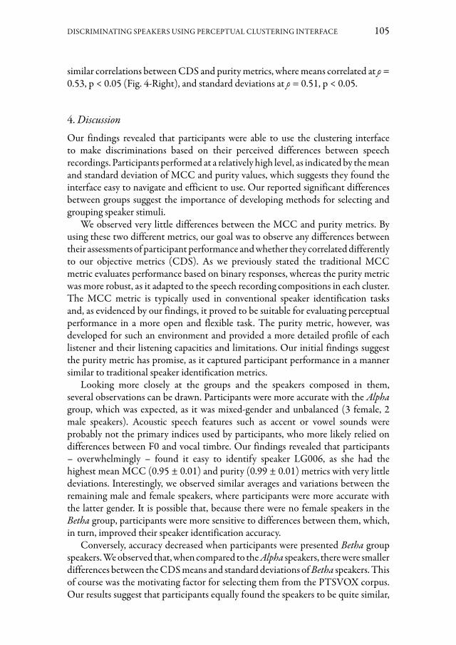
DISCRIMINATING SPEAKERS USING PERCEPTUAL CLUSTERING INTERFACE 105
similar correlations between CDS and purity metrics, where means correlated at ρ = 0.53, p < 0.05 (Fig. 4-Right), and standard deviations at ρ = 0.51, p < 0.05.
4. DiscussionOur findings revealed that participants were able to use the clustering interface to make discriminations based on their perceived differences between speech recordings. Participants performed at a relatively high level, as indicated by the mean and standard deviation of MCC and purity values, which suggests they found the interface easy to navigate and efficient to use. Our reported significant differences between groups suggest the importance of developing methods for selecting and grouping speaker stimuli.
We observed very little differences between the MCC and purity metrics. By using these two different metrics, our goal was to observe any differences between their assessments of participant performance and whether they correlated differently to our objective metrics (CDS). As we previously stated the traditional MCC metric evaluates performance based on binary responses, whereas the purity metric was more robust, as it adapted to the speech recording compositions in each cluster. The MCC metric is typically used in conventional speaker identification tasks and, as evidenced by our findings, it proved to be suitable for evaluating perceptual performance in a more open and flexible task. The purity metric, however, was developed for such an environment and provided a more detailed profile of each listener and their listening capacities and limitations. Our initial findings suggest the purity metric has promise, as it captured participant performance in a manner similar to traditional speaker identification metrics.
Looking more closely at the groups and the speakers composed in them, several observations can be drawn. Participants were more accurate with the Alpha group, which was expected, as it was mixed-gender and unbalanced (3 female, 2 male speakers). Acoustic speech features such as accent or vowel sounds were probably not the primary indices used by participants, who more likely relied on differences between F0 and vocal timbre. Our findings revealed that participants – overwhelmingly – found it easy to identify speaker LG006, as she had the highest mean MCC (0.95 ± 0.01) and purity (0.99 ± 0.01) metrics with very little deviations. Interestingly, we observed similar averages and variations between the remaining male and female speakers, where participants were more accurate with the latter gender. It is possible that, because there were no female speakers in the Betha group, participants were more sensitive to differences between them, which, in turn, improved their speaker identification accuracy.
Conversely, accuracy decreased when participants were presented Betha group speakers. We observed that, when compared to the Alpha speakers, there were smaller differences between the CDS means and standard deviations of Betha speakers. This of course was the motivating factor for selecting them from the PTSVOX corpus. Our results suggest that participants equally found the speakers to be quite similar,

106 B. O’BRIEN, C. MEUNIER, A. GHIO, C. FREDOUILLE, J.-F. BONASTRE, C. GUARINO
as indicated by the lower MCC means and higher standard deviations. All the Betha speakers were male, which suggests participants were required to be more sensitive in their listening in order to distinguish speakers. However, it was difficult to assess any inter- or intra-speaker discrimination strategies employed by participants. A study by Baumann and Belin (2008) reported that naïve listeners used F0 and mean difference between F4 and F5 different to identify male speakers. Future research could be conducted to assess whether there were any significant differences between these acoustic features across speakers. As provided in Tab. 1, we observed that both LG005 and LG017 speakers come from the Rhône region, so it is possible that participants perceived a likeness between them, which might have led to confusion that affected accuracy. This point is of course difficult to claim, given the limited stimuli and tests. However, it does bring into discussion the subject of accents in speaker identification task, which has become a recent research focus in the domain of computational linguistics (Hannani, Russell & Carey, 2013).
Turning to the results of our correlation procedures, we observed that an increase in speaker CDS mean lead to less accurate identifications, and, conversely, a decrease in speaker CDS standard deviation lead to an increase in speaker identification variability. These results suggest that ASV systems can be useful for preliminary speaker identification estimations by naïve listeners. A study by Gerlach et al. (2020) reported positive relationships between listener judgements and scores produced by ASV systems for both English and German language speakers. However, these findings contrast those reported in studies by Lindh, Eriksson (2010) and Zetterholm, Elenius & Blomberg (2004). Similarly, an important study by Park, Yeung, Vesselinova, Kreiman, Keating & Alwan (2018) found that not only did naïve listeners outperform an ASV system when completing a text-independent speaker discrimination task, but a weak correlation between human and machine performance. Taken these findings together suggest there are remain important differences in how humans and machines represent speakers.
The clustering task was designed to be more open in comparison to traditional perceptual speaker identification tasks. Both voice parades and pairwise comparisons restrict the modes in which users can express judgements. This differs from perceptual clustering tasks, which offer users dynamic engagements with speech materials. Rather than tasking listeners to judge whether a target speaker is present in a set (voice parade), the perceptual clustering method neutralises the concept of a “target” by asking them to organise a set of speech materials in terms of their likeness. It also provides naive listeners with a larger set of speech stimuli in which they could freely familiarise and group, which contrasts pairwise comparison method. While this study designed trials to include 20 speech stimuli, we have developed other studies with perceptual clustering tasks that include 12 (O’Brien, Meunier & Ghio, 2021a) and 15 speech stimuli (O’Brien, Chanclu, Tomashenko & Bonastre, 2021b). Moreover, a study by Lavan et al. (2021) found that a voice-sorting task provided familiar listeners with an advantage over unfamiliar listeners, which suggests listeners find any accessible information useful to evaluate speech materials.

DISCRIMINATING SPEAKERS USING PERCEPTUAL CLUSTERING INTERFACE 107
Although these findings revealed promising results, there are still many factors to consider for future work, such as the number of stimuli per session and the number of different speakers per group. Five different speakers were selected as it reflected a number typically used in a visual lineup. However, in an effort to remain balanced, it was possible that participants were able to correctly deduce that there were four speech recordings per group. To combat any (potential) deductions, we might consider developing an unbalanced design, where sessions are composed of an unequal number of speaker speech recordings. By contrast, we might change the task’s instructions, such that participants are asked to organise speech recordings into a maximum of four (or more) groups.
Unfortunately we were limited with the features we could measure with the interface. One feature that might offer additional insight is the number of times a participant listened to a speech recording, which could then be used to measure differences between participants and speakers. In addition, the number of times a speech recording was moved or classified might also support our analysis and provide us with a better parameter to measure the effects of the interface. These are some of the possibilities afforded by a clustering interface, which, when joined with other performance variables, could be used in combination for joint factorial analysis to better understand the interconnections between speaker discrimination performance and acoustic features that characterise speech.
5. ConclusionsOur perceptual clustering method highlighted how naïve listeners performed at a high level, which correlated to scores produced by our ASV system. Because of its design the perceptual clustering method produced idiosyncratic responses for each listener. In comparison to more restrictive perceptual speaker identification tasks, the clustering method could be used to not only profile listeners and understand better their perceptive capacities, but also to eliminate speech recording outliers, e.g. if certain recordings were too easily (mis)identified by listener populations. The selection of foil speech materials could be done in this manner, where ASV systems first select materials and, subsequently, listeners evaluate speech recordings via a perceptual clustering task to identify any biasing speech characteristics.
Overall, our results demonstrate that naïve listeners were effective at using the perceptual clustering task to identify speakers. This research led us to develop two different parallel speaker discrimination studies. As part of the same VoxCrim project, the first study examined the effects of different perceptual speaker identification tasks with similar stimuli (O’Brien et al., 2021a). This study centred on the voice parade, pairwise comparison, and clustering perceptual speaker identification tasks and examined the relationships between accuracy, task-dependent temporal features, and scores generated by an ASV system across and between tasks. Our findings from this study suggest that each perceptual task has the capacity to

108 B. O’BRIEN, C. MEUNIER, A. GHIO, C. FREDOUILLE, J.-F. BONASTRE, C. GUARINO
deliver important information that naive listeners can use when identifying and discriminating speakers.
A second study that employed a perceptual clustering method was part of the “VoicePrivacy Challenge,” collaborative, multi-objective project that aims to address questions surrounding speaker anonymization (Tomashenko, Srivastava, Wang, Vincent, Nautsch, Yamagishi, Evans, Patino, Bonastre, Noe, & Todisco, 2020). As part of this collaborative project, a study by O’Brien et al. (2021b) developed a more sophisticated clustering interface, which added some of the features mentioned above. Our goal was to examine the effectiveness of two different speaker anonymization systems. Like the current study, our findings showed participants were able to use the perceptual clustering method to link natural and anonymised speech recordings. Coupling these studies together, it is clear that a perceptual clustering method is robust and offers an innovative approach to studying voice perception.
AcknowledgementsThis work was funded by the French National Research Agency (ANR) under the VoxCrim project (ANR-17-CE39-0016). The authors thank the CEP staff (www.lpl-aix.fr/~cep), especially, Carine André, for assisting in the perceptual experiments.
Bibliography
Baumann, O., Belin, P. (2008). Perceptual scaling of voice identity: Common dimensions for different vowels and speakers. In Psychological Research, 74, 110–20.https://doi.org/75310.1007/s00426-008-0185-z.Belin, P., Bestelmeyer, P., Latinus, M. & Watson, R. (2011). Understanding Voice Perception. In British Journal of Psychology, 102, 711-725. https://doi.org/10.1111/j.2044-8295.2011.02041.x.Blatchford, H., Foulkes, P. (2006). Identification of voices in shouting. In International Journal of Speech, Language and the Law, 13(2), 241-254. https://doi.org/10.1558/ijsll.2006.13.2.241.Boë, L., Bonastre, J-F. (2012). L’identification du locuteur: 20 ans de témoignage dans les cours de Justice. Le cas du LIPSADON «laboratoire indépendant de police scientifique». Actes de JEP 2012, Grenoble, 4-8 June 2012, 417-424.Bonastre, J-F., Wils, F., Meignier, S. (2005). Alize, a free toolkit for speaker recognition. In Acoustics, Speech, and Signal Processing 1988, 737-740. https://doi.org/10.1109/ICASSP.2005.1415219.Broeders, T., Amelsvoort, A. (1999). Lineup Construction for Forensic Earwitness Identification: a Practical Approach. Proceedings of 14th International Congress of Phonetic Sciences, San Francisco, 1-7 August 1999, 1373-1376.Chanclu, A., Georgeton, L., Fredouille, C. & Bonastre, J.-F. (2020). PTSVOX: une base de données pour la comparaison de voix dans le cadre judiciaire. Actes de 6e conférence conjointe Journées d’Études sur la Parole, Nancy, 8-9 June 2020, 73-81.

DISCRIMINATING SPEAKERS USING PERCEPTUAL CLUSTERING INTERFACE 109
Dehak, N., Kenny, P., Dehak, R., Dumouchel, P., Ouellet, P. (2011). Front-End Factor Analysis for Speaker Verification. In IEEE Transactions on Audio, Speech, and Language Processing 19(4), 788–798. https://doi.org/10.1109/TASL.2010.2064307.Fleming, D., Giordano, B.L., Caldara, R. & Belin, P. (2014). A language familiarity effect for speaker discrimination without comprehension. In PNAS – Proceedings of the National Academy of Sciences of the United States of America, 111(38), 13795–13798. https://doi.org/10.1073/pnas.1401383111.Fredouille, C., Charlet, D. (2014). Analysis of I-Vector framework for Speaker Identification in TV-shows. In Proceeding of the 15th Annual Conference of the International Speech Communication Association, Interspeech 2014, Singapour, 14-18 September 2014, 71-75.Gaillard, P. (2009). Laissez-nous trier! TCL-LabX et les tâches de catégorisation libre de sons. In: Le sentir et le dire. Concepts et méthodes en psychologie et linguistique cognitives, L’harmattan (Coll. Sciences Cognitives).Gerlach, L., McDougall, K., Kelly, F., Alexander, A. & Nolan, F. (2020). Exploring the relationship between voice similarity estimates by listeners and by an automatic speaker recognition system incorporating phonetic features. In Speech Communication, 124, 85-95. https://doi.org/77810.1016/j.specom.2020.08.003.Gravier, G. (2021). Speech Signal Processing (SPro) Toolkit. https://www.irisa.fr/metiss/guig/spro.Hannani, A., Russell, M. & Carey, M. (2013). Human and computer recognition of regional accents and ethnic groups from British English speech. In Computer Speech & Language, 27(1), 59-74. https://doi.org/10.1016/j.csl.2012.01.003.Harris, M., Gries, S. & Miglio, V. (2014). Prosody and its application to forensic linguistics. In Linguistic Evidence in Security, Law and Intelligence, 2, 11-29. https://doi.org/10.5195/lesli.2014.12.Hollien, H., Bahr, R., Künzel, H. & Hollien, P. (2013). Criteria for earwitness lineups. In International Journal of Speech Language and the Law, 2(2), 143-153. https://doi.org/10.1558/ijsll.v2i2.143Hollien, H., Majewski, W. & Doherty, E.T. (1982). Perceptual identification of voices under normal, stress and disguise speaking conditions. In Journal of Phonetics, 10, 139-148.https://doi.org/10.1016/s0095-4470(19)30953-2Jenson, D., Saltuklaroglu, T. (2021). Sensorimotor contributions to working memory differ between the discrimination of same and different syllable pairs. In Neuropsychologia, Article 159. 107947. https://doi.org/10.1016/j.neuropsychologia.2021.107947.Jong, G., Nolan, F., McDougall, K. & Hudson, T. (2015). Voice lineups: A practical guide. Proceedings of the 18th International Congress of Phonetic Sciences, Glasgow, UK, 10-14 August 2015. https://www.internationalphoneticassociation.org/icphs-proceedings/ICPhS2015/Papers/ICPHS0598.pdfKanagasundaram, A., Vogt, R., Dean, D., Sridharan, S. & Mason, M. (2011). i-vector Based Speaker Recognition on Short Utterances. in Proceedings of the Annual Conference of the International Speech Communication Association, Interspeech 2001, Aalborg, Denmark, 3-7 September 2021, 2341-2344. https://doi.org/10.21437/Interspeech.2011-58.

110 B. O’BRIEN, C. MEUNIER, A. GHIO, C. FREDOUILLE, J.-F. BONASTRE, C. GUARINO
Kerstholt, J., Jansen, E., Amelsvoort, A. & Broeders, T. (2006). Earwitnesses: Effects of accent, retention and telephone. In Applied Cognitive Psychology, 20, 187-197. https://doi.org/10.1002/acp.1175.Kinnunen, T., Kilpeläinen, T. (2000). Comparison of clustering algorithms in speaker identification. Proceedings of IASTED International Conference on Signal Processing and Communications (SPC), Malaga, Spain, 19–22 September 2020, 222-227.Kreiman, J., Van Lancker Sidtis, D. (2011). Foundations of Voice Studies: An Inter-disciplinary Approach to Voice Production and Perception. Chichester, West Sussex, Malden, MA: Wiley-Blackwell.Larcher, A., Bonastre, J-F., Fauve, B., Lee, K, Levy, C., Li, H., Mason, J. & Parfait, J-V. (2013). ALIZE 3.0 – Open source toolkit for state-of-the-art speaker recognition. Proceedings of the Annual Conference of the International Speech Communication Association, Interspeech 2013, Lyon, France, 25-29 August 2013, 2768–2772.LaRiviere, C. (1971). Some acoustic and perceptual correlates of speaker identification. Proceedings of 7th International Congress of Phonetic Sciences, Montreal, Canada, 22-28 August 1971, 558-564.Lavan, N., Burston, L. & Garrido, L. (2018). How many voices did you hear? Natural variability disrupts identity perception from unfamiliar voices”. In British Journal of Psychology, 110, 576–593. https://doi.org/10.1111/bjop.12348.Lavan, N., Kreitewolf, J., Obleser, J. & McGettigan, C. (2021). Familiarity and task context shape the use of acoustic information in voice identity perception. In Cognition, 215, 104780. doi:10.1016/j.cognition.2021.104780Lindh, J., Eriksson, A. (2010). Voice similarity – a comparison between judgements by human listeners and automatic voice comparison. Proceedings, FONETIK 2010, Lund, Sweden, 2-4 June, 2010, 63-68.Lukic, Y., Vogt, C., Dürr, O. & Stadelmann, T. (2016). Speaker identification and clustering using convolutional neural networks. Proceeding of IEEE 26th International Workshop on Machine Learning for Signal Processing (MLSP), Vietri sul Mare, Italy, 13-16 September 2016, 1-6. https://doi.org/ 10.1109/MLSP.2016.7738816.Mattys, S. Davis, M., Bradlow, A. & Scott, S. (2012). Speech recognition in adverse conditions: A review. In Language and Cognitive, 27, 953-978. http://dx.doi.org/10.1080/01690965.2012.705006.Mühl, C., Sheil, O., Jarutyte, L. & Bestelmeyer, P. (2017a). The bangor voice matching test: A standardized test for the assessment of voice perception ability. In Behavior Research Methods, 50, 1-9. https://doi.org/10.3758/s13428-017-0985-4.Mullennix, J., Ross, A., Smith, C., Kuykendall, K., Conard, J. & Barb, S. (2011). Typicality effects on memory for voice: Implications for earwitness testimony. In Applied Cognitive Psychology, 25, 29-34. https://doi.org/10.1002/acp.1635.O’Brien, B., Meunier, C. & Ghio, A. (2021a). Presentation matters: Evaluating speaker identification tasks. Proceedings of the Annual Conference of the International Speech Communication Association, Interspeech 2021. https://doi.org/10.21437/Interspeech.2021-1211.O’Brien, B., Tomashenko, N., Chanclu, A. & Bonastre, J.-F. (2021b). Anonymous speaker clusters: Making distinctions between anonymised speech recordings with clustering interface. Proceedings of the Annual Conference of the International Speech Communication

DISCRIMINATING SPEAKERS USING PERCEPTUAL CLUSTERING INTERFACE 111
Association, Interspeech 2021, Brno, Czech Republic, 30 August – 3 September 2021, 3580-3584. https://doi.org/Interspeech.2021-1588.Öhman, L., Eriksson, A. & Granhag, P. (2010). Mobile phone quality VS. Direct quality: How the presentation format affects earwitness identification accuracy. In European Journal of Psychology Applied to Legal Context, 2(2), 161–182. www.usc.es/sepjfOlsson, J. (2003). What is Forensic Linguistics? England: Nebraska Wesleyan University.Park, S.J., Yeung, G., Vesselinova, N., Kreiman, J., Keating, P. & Alwan, A. (2018). Towards understanding speaker discrimination abilities in humans and machines for text-independent short utterances of different speech styles. The Journal of the Acoustical Society of America 144, 375-386. https://doi.org/10.1121/1.5045323.Roebuck, R., Wilding, J. (1993). Effects of vowel variety and sample length on identification of a speaker in a line-up. In Applied Cognitive Psychology, 7, 475–481. https://doi.org/10.1002/acp.2350070603.Salako, S.E. (2006). The Declaration of Helsinki 2000: Ethical Principles and the Dignity of Difference. In Medicine and Law, 2, 341-354. PMID: 16929810.Sloos, M., García, A-A., Andersson, A. & Neijmeijer, M. (2019). Accent-induced bias in linguistic transcriptions. In Language Sciences 76 (101176). https://doi.org/10.1016/j.langsci.2018.06.002.Smith, H., Baguley, T., Robson, J., Dunn, A. & Stacey, P. (2018). Forensic voice discrimination: The effect of speech type and background noise on performance. Applied Cognitive Psychology 33. doi:10.1002/acp.3478.Smith, H., Bird, K., Roeser, J., Robson, J., Braber, N., Wright, D. & Stacey, P. (2020). Voice parade procedures: optimising witness performance. In Memory 28(1), 9312-17. https://doi.org/10.1080/09658211.9322019.1673427.Stevenage, S. (2018). Drawing a distinction between familiar and unfamiliar voice processing: Are view of neuropsychological, clinical and empirical findings. In Neuropsychologia 116, 162-178. https://doi.org/10.1016/j.neuropsychologia.2017.07.005. Epub 2017 Jul 8. PMID: 28694095Stevenage, S., Symons, A., Fletcher, A. & Coen, C. (2019). Sorting through the impact of familiarity when processing vocal identity: results from a voice sorting task: familiarity and voice sorting. In Quarterly Journal of Experimental Psychology, 73. https://doi.org/10.1177/9391747021819888064.Tomashenko, N., Srivastava, B., Wang, X., Vincent, E., Nautsch, A., Yamagishi, J., Evans, N., Patino, J., Bonastre, J-F., Noe, P-G. & Todisco, M. (2020). Introducing the VoicePrivacy Initiative. Proceedings of the Annual Conference of the International Speech Communication Association, Interspeech 2020, Shangai, China, 25-29 October 2020, 1693-1697. https://doi.org/10.21437/Interspeech.2020-1333.Zetterholm, E., Elenius, D. & Blomberg, M. (2004). A comparison between human perception and a speaker verification system score of a voice imitation. Proceedings of the 10th Australian International Conference on Speech Sciences & Technology, Sydney, Australia, 8-10 December 2004, 393-397.


DOI: 10.17469/O2108AISV000006
THAYABARAN KATHIRESAN
Gender bias in voice recognition: An i- and x-vector-based gender-specific automatic speaker recognition study
One of the critical implications of the physiological differences between adult males and females is acoustic differences in speech production. Such acoustic signal variability between the genders affects automatic speech processing applications, especially automatic speaker recognition systems. In this paper, the performance of the genders in state-of-the-art automatic speaker recognition algorithms, such as i- and x-vector, is studied by training the algorithms using a gender-balanced multilingual dataset and tested with gender-separated data from two different languages (English and Mandarin). Furthermore, generated i- and x-vector speaker embedding distributions in higher-dimensions are analysed using the t-SNE technique. The area distribution of speaker embeddings aids interpretation of the speaker recognition performances for both algorithms.
Keywords: speaker recognition, i-vectors, x-vectors, gender-difference, speaker-embeddings.
1. IntroductionAutomatic speaker-recognition systems have emerged as an important means of verifying identity in many of today’s e-commerce applications, as well as in general business interactions, forensics, and law enforcement (Hansen, Hasan, 2015; Kahn, Audibert, Rossato & Bonastre, 2010). An ideal speaker recognition system models the identity of a speaker and later verifies the claimed identity of said speaker using her/his spoken utterance in any adverse conditions. In practice, the complexity of the speaker recognition model and the performance of the system are influenced by speaker variability such as age, gender, language, health, etc. (González Hautamäki, Hautamäki & Kinnunen, 2019).
In a long stream of speaker recognition research, extrinsic and intrinsic variations in the speech signal are major challenges. The most common extrinsic variations include diversity in recording device, ambient acoustics, background noise, transmission channel, and distortions introduced in pre-processing algorithms (Nagrani, Chung, Xie & Zisserman, 2020).
For instance, initial research was constrained to text-dependent tasks and focused on solving the variation caused by pronunciation randomness, for which the Hidden Markov Model (HMM) was the most popular (Parthasarathy, Rosenberg, 1996). Later research attempted to solve text-independent tasks and had to deal with phonetic variation, which gave rise to the Gaussian Mixture Model with Universal Background Model (GMM-UBM) architecture (Reynolds, Quatieri & Dunn, 2000). Further research tried to address inter-session variation caused by

114 THAYABARAN KATHIRESAN
channels and speaking styles, for which the i-vector/PLDA architecture was the most successful (Dehak, Kenny, Dehak, Dumouchel & Ouellet, 2011). Recently, the research focus has been targeted towards dealing with complex variations in the wild scenarios, for which deep learning methods (deep neural network or DNN) have been demonstrated to be the most powerful (Okabe, Koshinaka & Shinoda, 2018; Snyder, Garcia-Romero, Sell, Povey & Khudanpur, 2018; Variani, Lei, Mcdermott, Moreno & Gonzalez-Dominguez, 2014).
Interestingly, however, performance degradation due to intrinsic variations, also known as within speaker variability, has received far less attention even though it has a strong impact on ASV system performance (González Hautamäki et al., 2019; Kahn et al., 2010). Within speaker variability arises from the speaker and can include changes in pronunciation, speaking style, short-term health condition, emotion, and/or vocal effort (Karlsson, Banziger, Dankovicová, Johnstone, Lindberg, Melin, Nolan & Scherer, 1998). Besides, biological differences between males and females have consequences for the sounds they produce, such as the inner dimension of the mouth, throat, and vocal folds (Simpson, 2009). It is also clear that we make specific speech patterns appropriate to the gender; for example, male vocal folds tend to be longer and thicker than female vocal folds causing them to vibrate more slowly. As a result, male speakers have an average F0 of 131 Hz (Hertz, cycles per second), and females produce approximately twice the male frequency (220 Hz) (Hillenbrand, Clark, 2009). In this paper, we limit our research focus to voice identity between genders.
To overcome the gender differences in recognition system performance, the speaker recognition community has concentrated on designing gender-conditioned systems. One such system was introduced in 2011 using a mixture of Probabilistic Linear Discriminant Analysis models (PLDA) with i-vector systems to make systems independent of speaker gender (Senoussaoui et al., 2011). The system was tested on 2010 NIST telephone speech (det5). The experiment showed that the Equal Error Rate (EER%) for male speakers was relatively better (1.81 EER%) than female speakers (2.47%). A pairwise discriminative training procedure for i-vector-based speaker recognition, presented in 2012, equally showed system performance for male speakers was relatively better in all the system variants (Cumani, Glembek, Brümmer, Villiers & Laface, 2012). Recent findings suggest that DNN-based speaker recognition methods such as x-vector systems achieve excellent results. The gender-dependent and independent systems’ performance was tested using Kaldi-based x-vector techniques on SRE10 data, and the results show that the gender-dependent systems outperformed the independent systems (Snyder, Garcia-Romero & Povey, 2015). However, the gender-specific scores were not discussed in the paper.
In this current work, we study the impact of gender differences in i- and x-vector systems. In speaker recognition system design, we controlled the gender balance of data used in training the model and in testing the system. Moreover, we analyse speaker embeddings of both i- and x-vector systems using dimension

GENDER BIAS IN VOICE RECOGNITION 115
reduction techniques to understand the gender properties in high-dimensional embedding space.
The paper is organized as follows: Section 2 describes the i- and x-vectors, and we briefly recall the recognition scoring methods that have been used in the system evaluations. Section 3 presents the automatic speaker recognition experiment results and speaker embedding analysis. Finally, in Section 4, we discuss the findings and conclusion.
2. Methods2.1 Dataset
We used the multilingual speaker recognition corpora Voxceleb1 (Nagrani, Chung & Zisserman, 2017) and Voxceleb2 (Chung, Nagrani & Zisserman, 2018) to train the speaker recognition models. In both the Voxceleb1 and Voxceleb2 datasets, the number of male speakers is higher than the number of female speakers. To balance the gender, we randomly selected male speakers to balance the number of female speakers. The original and modified speaker counts are shown in Table 1.
Table 1 - Train dataset
Voxceleb1Original Modified
Voxceleb2Original Modified
#Total 1211 1092 5994 4402#Male 665 546 3793 2201
#Female 546 546 2201 2201
For testing, we used two datasets, TIMIT (English) (Garofolo, Lamel, Fisher, Fiscus & Pallett, 1993) and AISHELL-1 (Mandarin) (Bu, Du, Na, Wu & Zheng, 2017). Similar to the modifications made to the training data, we did a gender balance in the test data, shown in Table 2.
Table 2 - Test dataset
TIMITOriginal Modified
AISHELL-1Original Modified
#Total 630 384 400 372#Male 432 198 186 186
#Female 198 198 214 186
Though we used multilingual corpora for training the model, we used a language-specific (English and Mandarin) corpus for testing. The motivation is to explore the research question in a controlled speaker setting where we choose the language. In future studies, we will expand the question into more diverse and mixed language groups.

116 THAYABARAN KATHIRESAN
2.2 Automatic Speaker Recognition Algorithms
Both i- and x-vector systems were built using the Kaldi speech recognition toolkit (Povey, Ghoshal, Goel, Hannemann, Qian, Schwarz, Silovsk & Motl, 1968). We used a gender-balanced (see §2.1) version of Voxceleb1 and Voxceleb2 to train our recognition algorithms.
2.2.1 I-vectorAn i-vector system1 is a generative model that is derived using a total variability matrix (TVM) (Dehak et al., 2011). The TVM, obtained using unsupervised learning, is used to represent each utterance in a compact low-dimensional vector with an assumption that the speaker and session-dependent super vector M of Gaussian mean vectors may be modelled as
(1)
where m is the speaker and session-independent super vector obtained from a Gaussian mixture model (GMM) based universal background model (UBM), T is a low-rank total variability matrix that captures both speaker and session variability, and the i-vector is the posterior mean of w. The system is trained on 30 MFCC features with a frame-length of 25ms that are mean-normalized over a sliding window of up to 3 seconds. An energy-based speech activity detection (SAD) system selects features corresponding to speech frames. The UBM is a 2048 component full-covariance GMM. We extracted 400-dimensional i-vectors followed by an LDA scoring method (see §2.2.3).
2.2.2 X-vectorThe x-vector system2 is a time-delayed neural network architecture-based technique. We used 30-dimensional filter-banks with a frame-length of 25ms, mean-normalized over a sliding window of three seconds to train the x-vector system. Energy-based SAD (same as i-vector) is used to discard non-speech frames. We further applied augmentation on this data by adding music, speech, and noise using the MUSAN data set (Snyder, Chen & Povey, 2015); this consists of over 900 noises, 42 hours of music from various genres, and 60 hours of speech from twelve languages. This data augmentation helps the x-vector algorithm to be robust against noises and speech variabilities. Finally, we extracted 512-dimensional x-vectors followed by a PLDA scoring method (see §2.2.3).
2.2.3 Performance scoringThe results are presented in terms of equal error rate (EER), which corresponds to equal miss and false alarm rate. For both systems, linear discriminant analysis (LDA) is used to reduce the speaker embedding dimension. The LDA
1 Kaldi i-vector recipe at https://github.com/kaldi-asr/kaldi/tree/master/egs/voxceleb/v12 Kaldi x-vector recipe at https://github.com/kaldi-asr/kaldi/tree/master/egs/voxceleb/v2

GENDER BIAS IN VOICE RECOGNITION 117
dimensionality varies from 100 to 400 for i-vectors and 100 to 500 for x-vectors with 100 step-size. Further, the probabilistic linear discriminant analysis (PLDA) model is used for channel/session compensation and measuring EER scoring in our experiments.
3. ResultsFigure 1 - The speaker recognition performance (EER%) of the i-vector system
in 2 different datasets and different genders. The LDA -dimension is varied in the range of 100 to 400 with 100 step-sizes
We trained the recognition models (i- and x-vectors) with undifferentiated gender (gender-balanced and mixed), and the testing was carried out on gender-separated datasets. Overall, the x-vector system outperformed the i-vector system, as expected. Notably, both the training methods are showing similar performance trends between genders. The male speaker recognition scores are better than those for female speakers in both i- and x-vector systems independent of dataset and LDA-dimensions. For i-and x-vectors systems, changes in LDA dimension improve the overall performance of the AISHELL-1 dataset but have no impact on TIMIT i-vector systems (Fig. 1), and show counter effects in TIMIT x-vector systems (Fig. 2). Using a t-distributed stochastic neighbour embedding (t-SNE) (Van der Maaten, Hinton, 2008) dimension reduction technique, the dimension of extracted speaker embeddings from both i-vectors (400-dimension) and x-vectors (512-dimension) were reduced to two-dimensional vectors, as shown in Figs. 3 and 4.

118 THAYABARAN KATHIRESAN
Figure 2 - The speaker recognition performance (EER%) of the x-vector system in 2 different datasets and different genders. The LDA -dimension is varied in the range
of 100 to 400 with 100 step-sizes
Figure 3 - t-SNE reduced two-dimensional spaces of TIMIT speakers from i-vector (1) 400-dimension and x-vector (2) 512-dimension speaker embeddings
The male and female speakers were clustered, and the cluster area is measured by fitting a 95% confidence ellipse. The elliptical area for male and female speakers in both TIMIT (Fig. 3) and AISHELL-1 (Fig. 4) datasets for i- and x-vectors are shown below. We did 6-fold cross-validation (sub-figs. A till F as shown in Figs 3 and 4) on each dataset and each recognition algorithm to get a statistically valid cluster area measure. The cluster area of 6-fold cross-validation measured in i- and x-vectors of TIMIT and AISHELL-1 dataset is shown in Fig. 5. A 3-way ANOVA (Area as dependent factor and Gender, Dataset, and Recognition Type as independent factors) was performed. The main effects of Dataset [F (1,40) = 4.962, p=.0316] and Type [F (1,40) = 10.324, p=.0026] are significant. The interaction is significant between Dataset and Type [F (1,40) = 5.147, p=.0288], and Gender and Type [F (1,40) =25.034, p<.0001]. The three-way interaction is not significant [F (1,40) = .796, p=.3775].

GENDER BIAS IN VOICE RECOGNITION 119
Figure 4 - t-SNE reduced two-dimensional spaces of AISHELL-1 speakers from i-vector (1) 400-dimension and x-vector (2) 512-dimension speaker embeddings
Figure 5 - Cluster area of speaker embeddings from TIMIT and AISHELL-1 datasets in the 2-dimension t-SNE space
4. DiscussionOverall, the findings show that the performance of male speaker verification is better than that for female speakers, independent of the voice recognition algorithm and language of the dataset. These gender performance differences therefore corroborate findings from previous studies on gender-dependent and independent speaker recognition results (Cumani et al., 2012; Senoussaoui, Kenny, Brümmer, De Villiers & Dumouchel, 2011; Snyder et al., 2015: 92-97). In the current investigation, we controlled parameters such as the gender balance in training and testing data and LDA dimensions; however, the recognition performance difference between the gender was unaffected. Furthermore, the performance of the x-vector system is better

120 THAYABARAN KATHIRESAN
than the i-vector system as expected (Snyder et al., 2018), since the power of DNN makes it possible to capture subtle speaker-specific indexical information.
The t-SNE based speaker embedding analysis sheds some light on understanding the distribution of gender in higher-dimensional spaces. The idea of finding a correlation between algorithm performance and speaker embedding distribution has shown different effects in two different algorithms. The male speaker embedding in the i-vector space occupies a smaller area than that occupied by the female speakers. In contrast, the female speakers in the x-vector embedding space occupy a smaller area than male speakers. Fundamentally, the idea and mathematics behind i-vector and x-vector algorithms are different. There is seemingly no reason that both algorithms would model the speakers similarly. However, they have shown comparable effects across two different datasets, which paves the way for understanding the speaker embedding distribution properties with speaker recognition performance.
In future research, the acoustic feature extraction parameters such as frame length and number of MFCCs used to build the recognition models will be investigated to further understand the performance difference between the genders. In addition, we will explore the implications of the area of embedding distributions in the higher dimension (see Fig. 5) by manipulating the spread. Alternatively, some new perspectives about speaker individualities in a voice, like how individual speakers control their identity to some degree, are recently being discussed (Dellwo, Pellegrino, He & Kathiresan, 2019). These will also be considered in further studies to investigate the gender difference in speaker recognition performance.
AcknowledgementsThis work was supported by the Swiss National Science Foundation (SNSF), Grant No. 185399. I would like to thank Volker Dellwo for the support and supervision and Arjun Verma for his contributions in setting up the experiments. Also, I am grateful to Sandra Schwab for her contribution to the statistical analysis and Leah Bradshaw for proof reading.
Bibliography
Bu, H., Du, J., Na, X., Wu, B. & Zheng, H. (2017). AISHELL-1: An open-source Mandarin speech corpus and a speech recognition baseline. 20th Conference of the Oriental Chapter of the International Coordinating Committee on Speech Databases and Speech I/O Systems and Assessment O-COCOSDA, Seoul, South Korea, 1-3 September 2017, 1-5.Chung, J.S., Nagrani, A. & Zimmerman, A. (2018). Voxceleb2: Deep speaker recognition. Proceedings of the Annual Conference of the International Speech Communication Association, Interspeech 2018, Hyderabad, India, 2-6 September 2018, 1086-1090.Cumani, S., Glembek, O., BrÜmmer, N., De Villiers, E. & Laface, P. (2012). Gender independent discriminative speaker recognition in i-vector space. IEEE International

GENDER BIAS IN VOICE RECOGNITION 121
Conference on Acoustics, Speech and Signal Processing ICASSP, Kyoto, Japan, 25-30 March 2012, 4361-4364. doi: 10.1109/ICASSP.2012.6288885.Dehak, N., Kenny, P.J., Dehak, R., Dumouchel, P. & Ouellet, P. (2011). Front-End Factor Analysis for Speaker Verification. In IEEE Transactions on Audio, Speech, and Language Processing, 19(4), 788-798. https://doi.org/10.1109/TASL.2010.2064307.Dellwo, V., Pellegrino, E., He, L. & Kathiresan, T. (2019). The dynamics of indexical information in speech: Can recognizability be controlled by the speaker?. In AUC PHILOLOGICA, 2, 57-75. https://doi.org/10.14712/24646830.2019.18Garofolo, J.S., Lamel, L.F., Fisher, W.M., Fiscus, J.G. & Pallet, D.S. (1993). DARPA TIMIT acoustic-phonetic continous speech corpus CD-ROM. NIST speech disc 1-1.1. In NASA STI/Recon Technical Report N, 93.Gonzaléz HautamÄki, R., HautamÄki, V. & Kinnunen, T. (2019). On the limits of automatic speaker verification: Explaining degraded recognizer scores through acoustic changes resulting from voice disguise. In The Journal of the Acoustical Society of America, 146(1), 693-704. https://doi.org/10.1121/1.5119240.Hansen, J.H.L., Hasan, T. (2015). Speaker Recognition by Machines and Humans: A tutorial review. In IEEE Signal Processing Magazine, 32(6), 74-99. doi: 10.1109/MSP.2015.2462851Hillenbrand, J M., Clark, M.J. (2009). The role of f0 and formant frequencies in distinguishing the voices of men and women. In Attention, Perception, & Psychophysics, 71(5), 1150-1166. https://doi.org/10.3758/APP.71.5.1150Kahn, J., Audibert, N., Rossato, S. & Bonastre, J.F. (2010). Intra-speaker variability effects on Speaker Verification performance. Odyssey – Speaker and Language Recognition Workshop, Brno, Czech Republic, 28 June-1 July 2010, 109-116.Karlosson, I., Banziger, T., DankovicovÁ, J., Johnstone, T., Lindberg, J., Melin, H., Nolan, F. & Scherer, K. (1998). Within-speaker variability due to speaking manners. In 5th International Conference on Spoken Language Processing ICSLP, Sydney, Australia 30 November – 4 December 1998, 3(1), 2-5.Nagrani, A., Chung, J.S., Xie, W. & Zisserman, A. (2020). Voxceleb: Large-scale speaker verification in the wild. In Computer Speech and Language, 60, 101027. doi: https://doi.org/10.1016/j.csl.2019.101027.Nagrani, A., Chung, J.S. & Zisserman, A. (2017). VoxCeleb: A large-scale speaker identification dataset. Proceedings of the Annual Conference of the International Speech Communication Association, Interspeech 2017, Stockholm, Sweden, 20-24 August 2017, 2616-2620.Okabe, K., Koshinaka, T. & Shinoda, K. (2018). Attentive statistics pooling for deep speaker embedding. Proceedings of the Annual Conference of the International Speech Communication Association, Interspeech 2018, Hyderabad, India, 2-6 September 2018, 2252-2256.Parthasarathy, S., Rosenberg, A.E. (1996). General phrase speaker verification using sub-word background models and likelihood-ratio scoring. Proceeding of Fourth International Conference on Spoken Language Processing ICSLP, Philadelphia, USA, 3-6 October 1996, 2403-2406.

122 THAYABARAN KATHIRESAN
Povey, D., Ghosal, A., Goel, N., Hannemann, M., Qian, Y., Schwarz, P., Silovsk, J. & Motil, P. (1968). Sensory-perception testing box. In Canadian Journal of Occupational Therapy, 35(4), 140. PMID: 5195744.Reynolds, D.A., Quatieri, T.F. & Dunn, R.B. (2000). Speaker verification using adapted Gaussian mixture models. In Digital Signal Processing: A Review Journal, 10(1), 19-41. https://doi.org/10.1006/dspr.1999.0361.Senoussaoui, M., Kenny, P., BrÜmmer, N., De Villiers, E. & Dumouchel, P. (2011). Mixture of PLDA models in I-vector space for gender-independent speaker recognition. Proceedings of the Annual Conference of the International Speech Communication Association, Interspeech 2011, Florence, Italy, 27-31 August 2011, 25-28.Simposon, A.P. (2009). Phonetic differences between male and female speech. In Language and Linguistics Compass, 3(2), 621-640. https://doi.org/10.1111/j.1749-818X.2009.00125.xSnyder, D., Chen, G. & Povey, D. (2015). Musan: A music, speech, and noise corpus. In ArXiv Preprint: 1510.08484.Snyder, D., Garcia-Romero, D. & Povey, D. (2015). Time delay deep neural network-based universal background models for speaker recognition. IEEE Workshop on Automatic Speech Recognition and Understanding ASRU, Scottsdale, Arizona, USA, 13-17 December 2015, 92-97.Snyder, D., Garcia-Romero, D., Sell, G., Povey, D. & Khudanpur, S. (2018). X-Vectors: Robust DNN Embeddings for Speaker Recognition. IEEE International Conference on Acoustics, Speech and Signal Processing ICASSP, Calgary, Canada, 15–20 April 2018, 5329-5333.Van Der Maaten, L., Hinton, G. (2008). Visualizing Data using t-SNE. In Journal of Machine Learning Research, 2579-2605.Variani, E., Lei, X., Mcdermott, E., Moreno, I.L. & Gonzalez-Dominguez, J. (2014). Deep neural networks for small footprint text-dependent speaker verification. 2014 IEEE International Conference on Acoustics, Speech and Signal Processing ICASSP, Florence, Italy, 4-9 May 2014, 4052-4056.
DOI: 10.17469/O2108AISV000007
MARCO FARINELLA, MARCO CARNAROGLIO, FABIO CIAN
Una nuova idea di “impronta vocale” come strumento identificativo e riabilitativoA new concept of “voiceprint” as identification and rehabilitation tool
The concept of voiceprint always arouses many perplexities: it has been criticized several times in the past and it has therefore been archived. What if we made a mistake? In this study we tried to make a completely innovative use of it, observing it from a new perspective. We analysed the voices of more than a thousand subjects. We divided the spectrum of the voice into four categories, extrapolating refined biological information. In particular we analysed the adduction of the vocal cords, the use of the oral cavity, the mucosal wave and the physiological aspects of the apparatus. This new idea of voiceprint has proved to be an unexpectedly effective rehabilitation tool. We do not rule out that it may be reconsidered for use in forensic field in the future.
Keywords: voiceprint, FFT, laryngeal stress, identity, rehabilitation.
1. IntroduzioneLa voce dell’uomo è un fenomeno fortemente correlato alla sua identità. Le sensa-zioni provate, l’educazione ricevuta, le esperienze passate, la psicologia, le convin-zioni raggiunte, la cultura acquisita, le condizioni fisiche, le intenzioni, le credenze, le emozioni e molto altro sono elementi che indubbiamente caratterizzano il parla-to. Tuttavia, analizzando unicamente il processo fisico, possono essere sussunti gli elementi significativi che intervengono nel processo fonatorio. Essi sono: il cervello che determina il programma motorio, il corpo fisico che produce il fenomeno vi-bratorio e la voce, ovvero l’evento sonoro finale. I tre ambiti sono stati ampiamente indagati dal punto di vista scientifico da svariate discipline che, da un lato, hanno permesso di comprenderne i meccanismi di base e, dall’altro, hanno messo in luce la complessità del fenomeno e la necessità di nuove forme di approccio concettuale e strumentale.
Sappiamo che il connettoma, cioè l’organizzazione strutturale e funzionale di neuroni e sinapsi fra aree corticali e subcorticali (White, Southgate, Thomson & Brenner, 1986; Varshney, Chen, Paniagua, Hall & Chklovskii, 2011) è un mecca-nismo assai articolato che, oltre ad occuparsi della gestione pratica dei movimenti, racchiude anche intricati aspetti psicologici ed emotivi. L’effetto di questi ultimi elementi sul sistema nervoso è noto da lungo tempo perché rappresenta il tema prin-cipale nell’Arte che, da sempre, ne sfrutta l’impatto emozionale pur avendo solo una conoscenza superficiale della fisiologia che ne sta alla base.

124 MARCO FARINELLA, MARCO CARNAROGLIO, FABIO CIAN
La foniatria e la logopedia, invece, hanno approfondito scientificamente la vocalizzazione umana, puntando costantemente la propria attenzione sui mecca-nismi patologici. Ciò ha permesso di comprendere e correggere molte delle di-sfunzioni legate alla voce ma ha portato anche a trascurare parzialmente gli aspetti eufonici ed eutonici della prestazione. Di conseguenza, gli studi sulla funzionalità laringea risultano molto rari, datati e deficitari. Inoltre i soggetti-cavia coinvolti sono quasi sempre poco numerosi e sottoposti ad osservazioni di durata limitata (Stolze, 1995).
Infine, la fisica acustica si è occupata di analizzare minuziosamente il fenomeno sonoro, scomponendo la voce in parametri sempre più dettagliati e precisi (Kelly, Forth, Kent, Gerlach & Alexander, 2019). Questo tipo di pensiero ha certamente aperto nuovi orizzonti sulla concezione del segnale audio, però ha altresì reso fati-coso definire con certezza l’identità del parlante, le sue emozioni ed ancor più le sue intenzioni e sensazioni, parametri che richiedono chiavi di lettura interdisciplinari di notevole difficoltà. Tutto questo impone che si avvicendino ricerche ininterrotte e che si aprano continui dibattiti sui risultati raggiunti, al fine di arrivare ad accerta-re uno standard di analisi che possa essere preciso, veritiero e condivisibile (Hamidi, Satori, Laaidi & Satori, 2020).
La decodifica della voce è comunque materia antica. Da sempre l’uomo usa il proprio istinto empatico per decifrare i segnali verbali della comunicazione, nel tentativo di riconoscere i propri simili, comprenderne le intenzioni o svelarne le menzogne. In molte epoche, vicine e lontane, le parole sono state usate come armi investigative, spesso strumentalizzandole in interpretazioni apofeniche, come è suc-cesso nei periodi più bui della recente storia dell’uomo e sotto le dittature. È però inammissibile, in sede giudiziaria, che l’opinione soggettiva abbia rilevanza ai fini processuali. Ecco perché, con l’avvento della tecnologia, è diventato indispensabile studiare metodi efficaci per identificare la falsità, appagando così la necessità di una valutazione super partes adatta ad un’aula di tribunale (IlPost.it, 2015).
Inizialmente l’attenzione si è rivolta verso gli effetti secondari legati alla fisiolo-gia. Tralasciando i primi maldestri tentativi di Angelo Mosso e Cesare Lombroso, possiamo datare il poligrafo moderno (più volgarmente chiamato macchina della verità) al 1913, quando è nato per mano di William Moulton Marston, venendo poi successivamente perfezionato da Larson. Purtroppo la sua efficacia non è mai stata dimostrata pienamente (De Cataldo Neuburger, 2007; Germanà Tascona, 2005) e, per questo motivo, è rifiutato come prova dall’ordinamento giuridico moderno, sebbene sia tollerato da alcune giurisdizioni statunitensi come prova indiziaria, quando concordata fra le parti.
L’interesse degli addetti ai lavori si è quindi inevitabilmente spostato verso il suono e, in particolare, sull’impronta vocale. Timbro, intonazione, posizione degli accenti, velocità di elocuzione, durata ed epentesi vocalica e consonantica, variazio-ne intra e interlinguistica sono diventati i nuovi campi di ricerca (Saleem, Subhan, Naseer, Bais & Imtiaz, 2020). Numerosi studi hanno indagato tutti questi parametri utilizzando la stima della frequenza, i modelli di misture gaussiane (GMM) e quel-

UNA NUOVA IDEA DI “IMPRONTA VOCALE” 125
li di Markov nascosti (HMM), gli algoritmi di pattern matching, le reti neurali, le matrici di rappresentazione, la quantizzazione vettoriale e gli alberi di decisione. Tuttavia, nonostante le varie teorie formulate e le tecniche utilizzate (cohort model, modelli ambientali, algoritmi di riduzione del rumore, etc...), permangono molti problemi (Zetterholm, 2003). Le condizioni di ripresa, i sottofondi ambientali, i comportamenti, le inflessioni linguistiche, gli umori, lo stato di salute e l’età del sog-getto possono infatti inficiare sia la fase di raccolta, sia quella di verifica degli elemen-ti, rendendo alquanto controversa la qualità dei risultati ottenuta elettronicamente (Gold, French, 2019). In ambito forense ciò rende indispensabile l’affiancamento di esperti con abilità d’ascolto specifiche (Romito, Galatà, 2008) affinché l’esito dell’analisi possa ritenersi accettabile in termini probabilistici (Grimaldi, d’Apolito, Gili Fivela & Sigona, 2014). L’impronta vocale è stata quindi abbandonata come indice di riconoscimento in favore di un calcolo matematico che possa orientare una giuria riguardo all’identità di un parlante, lasciando alla disamina umana qualsiasi giudizio in merito alla veridicità del contenuto a cui si rifà la conversazione (Tonini, 2005). Questo contributo quindi, utilizzando un vecchio strumento, propone una diversa interpretazione del fenomeno sonoro durante la verbalizzazione, nell’atte-sa che la scienza individui metodologie d’integrazione fra le letture strumentali e la percezione umana che possano affiancare, in maniera affidabile, l’indispensabile apporto del tecnico forense.
2. Scopo del lavoroLo scopo del presente lavoro è approfondire la correlazione fra l’intera gamma di frequenze emesse con la voce umana e la fisiologia che l’ha prodotta, per indivi-duare una configurazione atta ad identificare e migliorare gli aspetti funzionali ed emotivi peculiari di una persona. Ciò permette di dare nuova vita al superato con-cetto di impronta vocale che, opportunamente mappata (alla stregua del genoma umano) potrebbe svelare, con precisione sorprendente, peculiarità fisiche ed emo-tive di un soggetto.
3. Prima fase3.1 Premessa
Partendo dal presupposto che l’uomo riproduce con la voce soltanto ciò che riesce ad udire (Tomatis, 1987) e lo fa attraverso un procedimento esclusivamente bio-logico, l’idea è di trovare una stretta correlazione fra l’intero spettro sonoro e la fisiologia che lo ha prodotto, individuando così una personale impronta acustica.
Se il tratto vocale maschile fosse un cilindro ricurvo, di sezione costante, la sua risonanza sarebbe caratterizzata perlopiù da modi dispari a partire da 500 Hz. Nel caso di voci femminili o di bambini la fondamentale risulterebbe un po’ più acuta ma seguente la stessa logica. Nella realtà si aggiungono l’oscillazione delle corde vo-

126 MARCO FARINELLA, MARCO CARNAROGLIO, FABIO CIAN
cali (diverse da individuo a individuo) che caratterizza la nota fondamentale emessa e la deformazione volontaria del tratto che sposta le formanti vocaliche dando leg-gibilità al linguaggio. Il processo si completa con l’onda della mucosa che produce armonici sopracuti in funzione della dinamica e della tensione cordale, nonché del contributo delle cavità del cranio che possono filtrare, rinforzare o assorbire una vasta gamma di frequenze in base al loro utilizzo.
Di conseguenza, considerando la regione anatomica, il corpo vibrante, le moda-lità di risonanza, la pressione aerobica e quella muscolare è dunque possibile indivi-duare precise correlazioni fra essi e lo spettro di Fourier, il quale denuncia così non solo la presenza frequenziale del fenomeno sonoro ma anche le condizioni psicobio-logiche del corpo che le ha prodotte (Rohmert, 1995).
3.2 Raccolta dati
Fra il 2003 e il 2020, attraverso un’osservazione funzionale, si è indagato l’atteggia-mento laringeo (seguendo i principi espressi da Rohmert, 1981) di un campione composto da 1061 persone (33% uomini e 67% donne) nell’atto della fonazione. Le età medie sono state di 47 anni (fra i 7 e i 91 anni) per i maschi e di 48 anni (fra i 12 e gli 85 anni) per le femmine.
Le condizioni di ascolto delle singole voci sono state omogenee nel complesso ed identiche per gruppi di 10-12 persone circa. La strumentazione utilizzata per le analisi è comprensibilmente variata nel corso dei 17 anni di ricerca, adeguandosi al progredire della tecnologia ma tutte le attrezzature impiegate (hardware e software) sono sempre state di fascia professionale e manovrate da operatori qualificati.
Inoltre, avendo a disposizione i soggetti (e non semplicemente registrazioni di conversazioni telefoniche) le principali analisi effettuate riguardano: la determina-zione della frequenza fondamentale (f0) e dell’ampiezza di emissione vocale ed il re-lativo andamento nel tempo (curva di intonazione e di intensità); l’identificazione delle perturbazioni del periodo fondamentale (Jitter) e dell’ampiezza (Shimmer), lo studio del bilancio energetico spettrale (rapporto fra componente periodica ed ape-riodica nel segnale: Harmonic to Noise Ratio), il calcolo della presenza di diplofonia (semplice o multipla) e degli arresti momentanei dell’emissione (Vocal Breaks), non-ché la fonetografia per l’identificazione dell’estensione e tessitura vocale.
Le caratteristiche acustiche delle voci sono state raffrontate con la condizione di salute fisica e psicologica, con le abitudini sociali e i comportamenti professionali degli individui esaminati. Per praticità di elaborazione dei dati l’intera gamma delle frequenze udibili dall’uomo è stata suddivisa nelle seguenti aree (identificative della regione anatomica in cui si sviluppano): suono fondamentale (prodotto dalle pliche vocali), formanti vocaliche (proprie della cavità orale), brillantezza sonora (influen-zata dall’onda della mucosa), sopracuti funzionali (frutto della fisiologia degli appa-rati) (Rohmert, Rehders & Rohmert, 1990).

UNA NUOVA IDEA DI “IMPRONTA VOCALE” 127
Figura 1 - In rosso lo spettro di Fourier di una voce maschile che pronuncia la frase “le mie aiuole”. In nero la suddivisione delle aree frequenziali per l’analisi vocale
3.3 Analisi ed elaborazione dei dati
I risultati più interessanti sono derivati dalla tradizionale analisi prosodico-intona-tiva applicata però a tutte le aree, monitorando quindi la derivata di f0 e dell’intera gamma di armonici nelle bande di maggiore rilevanza. Le indagini sono servite per enucleare un pattern sonoro ideale, di perfetto funzionamento laringeo, da attribuire ad un ipotetico adulto, in perfetta salute, scevro da traumi fisici e psicologici, in con-dizioni emotive di equilibrata serenità. Utilizzando un passaggio d’aria durante il meccanismo di rilassamento della chiusura glottale (Greene, Mathieson, 2001) è sta-ta misurata la risonanza laringea a riposo di ogni partecipante. Questa indagine ha avuto esiti con risultati sostanzialmente sovrapponibili indipendentemente dal nu-mero di misurazioni eseguite per singolo soggetto. A questo riferimento teorico si è attribuito un valore arbitrario di affaticamento glottico pari allo 0%. Comparando statisticamente le trasformate di Fourier (FFT) reali dell’intera frase concordata (“le mie aiuole”) con il modello ideale si sono evidenziate le discordanze dovute alle co-strizioni laringee tipiche di ciascun soggetto considerato, attribuendo ad ognuno un valore di affaticamento vocale espresso in percentuale. Tale punteggio rappresentava la condizione fonatoria quotidiana dell’individuo, nel periodo osservato, generan-do anche una nuova concezione di impronta vocale più vicina a fattori biologici che ad elementi linguistici (Lindh, 2004).

128 MARCO FARINELLA, MARCO CARNAROGLIO, FABIO CIAN
3.4 Risultati (prima fase)
L’idea di dare una nuova vita al concetto di impronta vocale si è dimostrata sensata. Lavorando con voci analizzate a pieno spettro si è potuto attingere ad una ricchezza frequenziale impensabile per le conversazioni telefoniche. Ciò ha permesso di identificare delle correlazioni sonore con la biologia dei parlanti che normalmente vengono trascurate in ambito forense e considerate solo in campo medico in relazione alle patologie.
Paragonando quindi l’intero spettro sonoro delle voci con la FFT ideale si è determinato il grado di funzionalità delle prestazioni vocali senza ricorrere ai tradizionali esami clinici che, per la loro complessità, sono eseguibili soltanto in apposite strutture sanitarie con personale qualificato. Questo, di fatto, ha snel-lito notevolmente la procedura. Inoltre, si è evidenziato come la percentuale di discostamento dal modello di riferimento tenda a mantenersi costante per ogni esaminato a parità di condizioni psicofisiche, caratterizzando quindi l’oratore, pur non essendo ancora riusciti a parametrizzare la lettura strumentale per il riconoscimento univoco del parlante senza l’intervento umano.
4. Seconda fase4.1 Premessa
Per valutare la qualità dei dati raccolti e la bontà delle conclusioni, si è deciso di eseguire un secondo test sul modello di riferimento appena individuato. Si è provato quindi ad invertire l’ottica d’indagine e, fra il 2005 e il 2011, 171 vo-lontari sono stati sottoposti ad un’unica stimolazione percettiva che inducesse la loro voce ad assomigliare al pattern sonoro ideale. Le persone impiegate nell’e-sperimento sono state per il 30% uomini e 70% donne con una età media di 45 anni in entrambi i sessi. Il reclutamento dei volontari è avvenuto volutamente in maniera casuale all’interno delle seguenti categorie professionali: insegnan-ti, artisti, casalinghe, disoccupati, professionisti, manager e dirigenti, impiegati, imprenditori, operatori sanitari, medici, psicologi, rieducatori, doppiatori, ope-ratori dello spettacolo, sportivi, personal trainer, formatori. Circa il 50% di essi necessitava di rieducazione, il restante 50% partiva da una condizione di salute. Tutti i partecipanti erano accomunati da uno spiccato interesse per la voce (par-lata o cantata).
4.2 Raccolta ed elaborazione dei dati
I dati sono stati raccolti da gruppi eterogenei di 10-12 persone convocate per singola seduta. Prima di iniziare, ogni partecipante ha compilato un questiona-rio riguardante il proprio stato emotivo e sensoriale. Per la valutazione è stato usato un test con venticinque coppie di aggettivi contrapposti (ispirato a Costa, McCrae, 1992), disposti in maniera casuale. Il modulo per l’indagine è stato preparato da una psicologa professionista esterna alla struttura, nel rispetto

UNA NUOVA IDEA DI “IMPRONTA VOCALE” 129
di tutti i criteri necessari e convenzionalmente accettati per la corretta stima dei risultati. Il gruppo è stato poi sottoposto ad un training uditivo intensivo (Rohmert, 1990). Ad ogni aderente è stato chiesto di vocalizzare singolarmente per 45 minuti durante i quali il proprio ascolto è stato sollecitato dai parametri funzionali identificati nel pattern sonoro (Rohmert, 1991). L’idea era di elicita-re sensorialmente le voci verso un punto zero fisiologico di affaticamento e son-darne la retroazione, funzionale ed emotiva, impattante sulla percezione del sé, sull’identità e sul conseguente modello comportamentale. La percezione delle formanti, unita alle stimolazioni binaurali, monaurali e sincroniche hanno pro-gressivamente codificato il suono parlato e cantato dei soggetti cavia. Sfruttando il concetto di sintonizzazione cerebrale decodificato all’Università di Cambridge (Leong, Byrne, Clackson, Georgieva, Lam & Wass, 2017) si è assistito ad una modificazione plastica della struttura cerebrale degli aderenti con l’attivazione di onde Alpha (8-13 Hz), Theta (4-7 Hz) e Delta (<3,5 Hz) rilevabili da elettro-encefalogramma (EEG). Al termine l’intero gruppo è stato nuovamente invitato a compilare, in forma anonima, il test riguardante la percezione soggettiva, emo-tiva e sensoriale dell’esperienza vissuta.
4.3 Risultati (seconda fase)
Il risultato certamente più sorprendente si è raggiunto utilizzando il pattern vo-cale ideale come stimolazione per il miglioramento della prestazione fonatoria. Infatti l’esito dell’esperimento ha messo in luce la sua grande capacità rieduca-tiva (priva di effetti collaterali) e la forte retroazione sull’identità dei volontari stimolati. L’affaticamento glottico si è notevolmente ridotto ed i test psicologici hanno conseguentemente evidenziato una variazione drastica del quadro emoti-vo, con due importanti traguardi: l’eliminazione dei vocaboli con un’accezione negativa nella descrizione del proprio stato psicofisico (ad es. teso, pesante, stan-co, triste...) ed un incremento della propriocezione dei soggetti verso gli aggetti-vi positivi (attivo, riposato, allegro, concentrato...) con percentuali di migliora-mento che vanno dal 6% fino al 53%, con una media globale di poco inferiore al 30% ottenuta in un’unica seduta di stimolazione.

130 MARCO FARINELLA, MARCO CARNAROGLIO, FABIO CIAN
Figura 2 - In blu la condizione emotiva dei soggetti prima della stimolazione, in rosso il cambiamento propriocettivo al termine della seduta
5. ConclusioniOggi la comunicazione rappresenta oltre il 50% dei problemi della nostra società al punto che è considerata anche il fattore critico delle strategie d’impresa delle aziende (Passerini, Tomatis, 2007). Il motivo è che ormai ci troviamo ad abitare un mon-do caratterizzato da un eccessivo rumore di fondo, un frastuono d’informazioni in cui tutti gridano la propria verità e in cui è quasi impossibile distinguere la qualità del messaggio. “Paradossalmente, l’ipercomunicazione ha creato un blocco della co-municazione stessa. Più si grida, meno si comunica e meno ci si capisce” (Passerini, Tomatis, 2007: 17). Nella società di oggi, oltre alle sordità fisiche e psicologiche (sia nei confronti dell’ambiente circostante, che di se stessi), siamo arrivati a quantificare i danni prodotti persino da un inquinamento semiotico, caratterizzato da nuove ma-lattie sociali, come il “Tautismo: un autismo tautologico” (Passerini, Tomatis, 2007: 18), una sorta quindi di impossibilità di comprendersi. È facile immaginare cosa ab-bia creato questa difficoltà di comunicazione nelle aule di tribunale (Grevi, 2003).
Arrivati ormai alla babele si è cercato in tutti i modi di tornare a capirsi, risco-prendo la semantica delle parole, mutuando termini da altre lingue e persino co-niando nuovi vocaboli. Nulla però è servito a riportare una piena comprensione del prossimo perché è impossibile arrivare ad interagire efficacemente con gli altri se prima non si giunge a conoscere appieno la propria capacità percettiva. Solo così un dialogo può diventare un rapporto profondo fatto di parole essenziali. Infatti,

UNA NUOVA IDEA DI “IMPRONTA VOCALE” 131
all’interno di una buona comunicazione è importante tenere conto del fattore sog-gettivo di chi emette e di chi riceve l’informazione. “Nei processi comunicativi esi-ste una sorta di autocomunicazione” (Passerini, Tomatis, 2007: 30) che ha a che fare più con il nostro “percepito” che con la realtà. Si potrebbe dire quindi che le per-sone, più che vere informazioni, si scambiano continuamente impressioni. Questo aspetto è ciò che maggiormente mina la comprensione della voce umana, diventan-do anche un fattore invalidante nel caso di analisi strumentali (Zetterholm, 2003). Migliorare consapevolmente l’ascolto è, allora, l’unica possibilità che un tecnico forense ha per svelare il vero senso della comunicazione.
Ne consegue che l’attenzione degli studiosi si è concentrata sulle caratteristi-che del suono emesso, tentando di individuare le affinità che intercorrono fra la voce umana e la rosa di emozioni che guida gli atteggiamenti. Da subito la mate-ria ha rivelato tutta la sua complessità rendendo particolarmente arduo il compito (Federico, Paoloni, 2007). Si è tentato quindi di riferirsi ad elementi che potessero essere più facilmente identificabili e che potessero diventare indici per il riconosci-mento delle emozioni in corso. Tuttavia, la percezione umana è assai complessa. L’uomo infatti può incamerare fino a 60 milioni d’informazioni al secondo, an-che se le persone mediamente ne traggono, dall’ambiente circostante, appena 2-3 mila ed il loro cervello cosciente riesce a gestirne contemporaneamente soltanto 5-9 (Miller, 1956). Da questi numeri si evince quanto qualunque azione istintiva possa essere più efficace rispetto a qualsiasi atto tecnico volontario. Il nostro principio base, dunque, è quello di attingere alla ricchezza delle risorse istintive dove si trova il 95% dei dati utili ad innescare reazioni automatiche. Dei 60 milioni di informa-zioni al secondo che l’uomo riceve il 54% riguarda il corpo fisico e solo il 46% viag-gia attraverso il suono. Di conseguenza il linguaggio corporeo viene spesso preso come principale indicatore nelle analisi comportamentali ed emotive. Tuttavia, in questo 54%, ad eccezione di una piccola parte di indicatori (che riguarda il colore della pelle, la quantità di sudorazione, etc...), la maggior parte delle informazioni è facilmente travisabile se non addirittura manipolabile, in primis la postura, come in-segnano le tecniche di comunicazione aziendale. Il residuo 46% delle informazioni invece, spesso trascurato e decisamente sottovalutato, viene trasportato dal suono. Qui, soltanto il 7%, che si riferisce al valore semantico delle parole, è di fatto mani-polabile e possibile fonte di menzogna, mentre il restante 39% riguarda suoni non verbali, istintivi, che difficilmente si prestano alla falsità. In questo ambito vengono esplicitati anche i bisogni più intimi ed i pensieri più nascosti. Si tratta quindi di una preziosa rappresentazione sensoriale, dinamica e sinergetica dell’organizzazio-ne cerebrale dell’interlocutore, al punto che si potrebbe parafrasare il vecchio detto “dimmi come parli e ti dirò chi sei!”.
Imparare a leggere l’impronta vocale, quindi, risulta una risorsa preziosissima, considerato che essa trasporta oltre 26 milioni di informazioni al secondo, di na-tura purissima! Di fronte a numeri del genere è impossibile, per chiunque debba analizzare una voce, non soffermarsi a riflettere sull’importanza del saper dirigere adeguatamente la propria attenzione uditiva sulle frequenze che la caratterizzano

132 MARCO FARINELLA, MARCO CARNAROGLIO, FABIO CIAN
e sui relativi parametri maggiormente ricchi di significato. Il timbro vocale è una precisa e scrupolosa carta d’identità che mostra al nostro interlocutore una real-tà che va oltre le parole pronunciate. Considerando poi che il suono, a differenza dell’impronta digitale, oltre ad identificare il soggetto ne definisce dettagliatamente anche ogni sua sensazione, atteggiamento e attitudine, comprendere i segnali vocali diventa uno strumento più che mai necessario in ambito forense.
Durante una deposizione tutto ciò che avviene si fa principalmente con la voce. Occorre tener presente che scambiare informazioni durante un colloquio non si-gnifica necessariamente comunicare. La vera comunicazione, infatti, fa leva sulle in-tenzioni inconsce prima ancora che diventino azioni e lo fa attraverso un profondo processo di comprensione, mettendo al centro dell’attenzione i propri interlocutori. In questo scenario saper ascoltare e, di conseguenza interagire, risulta quindi fon-damentale per accertare la verità. Il tecnico forense non dovrebbe giudicare il con-tenuto della dichiarazione, compito per il quale viene deputata un’apposita giuria. Per colui che è designato ad analizzare i parametri sonori è indispensabile tornare a dare voce a tutti i livelli di comunicazione, svelando il piano biologico alla stregua di quello culturale. Del resto, se l’era dell’ipercomunicazione oggi ci impone di riscopri-re la genuinità del messaggio, perché non fare il passaggio successivo abbracciando la neuro-comunicazione anche in tribunale?
La voce, nel ventaglio delle sue ventimila frequenze e grazie agli oltre ventisei milioni di informazioni empatiche al secondo che esse portano con sé, è certamen-te ascrivibile all’identità individuale della persona. È quindi necessario imparare a leggerla in tutto il suo contenuto. La muscolatura del tratto vocale reagisce istintiva-mente alle emozioni come primaria difesa dei polmoni. Questo fa sì che la risonanza di ogni persona sia diversa e assimilabile ad un’impronta digitale. Il vissuto di un in-dividuo resta registrato nella sua biologia, caratterizzandone la personalità emotiva, comportamentale e quindi anche quella sonora globale. Per esaminare la condizione psicofisica di un individuo si ritiene pertanto necessario considerare l’intera confi-gurazione frequenziale, valutando il differenziale della sua impronta vocale di una intera asserzione (intesa nell’accezione del presente studio) da una trasformata di Fourier ideale. Perfezionando questa tecnica, non si esclude una futura applicazione in ambito forense, non tanto per validare le intercettazioni (normalmente troppo disturbate da rumori parassiti che interferiscono con l’esame audio), quanto per va-lutare il grado di stress laringeo durante una dichiarazione giurata. L’incremento di tensione muscolare nel pronunciare una frase (rilevato paragonando l’analisi della voce durante una deposizione con la propria impronta laringea) potrebbe risultare assai prezioso, come parametro oggettivo, per stimare la veridicità di una dichiara-zione. Tuttavia, in attesa di creare una procedura automatizzata e sicura per l’osser-vazione tecnica ipotizzata, questa nuova concezione di impronta vocale ideale può già essere utilizzata con successo come strumento riabilitativo, sia dal punto di vista fisiologico, sia psicologico (Rohmert, 1989). Infatti, quando è impiegata come mo-dello acustico all’interno di una pedagogia sensorialmente orientativa, essa è in grado di rieducare velocemente una funzione glottica deficitaria e di retroagire fortemente

UNA NUOVA IDEA DI “IMPRONTA VOCALE” 133
sull’umore, con effetti duraturi di miglioramento sulla percezione del sé. La voce così riabilitata aumenta il suo grado di funzionalità fisiologica e l’identità delle per-sone trattate risulta più definita, equilibrata e risoluta.
Riferimenti bibliografici
Costa, P.T., McCrae, R.R. (1992). NEO PI-R professional manual. Odessa: Psychological Assessment Resources.De Cataldo Neuburger, L. (2007). La prova scientifica nel processo penale. Padova: Cedam.Federico, A., Paoloni, A. (2007). Riconoscimento del parlante. In Media Duemila, 250, 47-55.Germanà Tascona, N. (2005). Sub art. 188. In Corso, P. (a cura di). Commento al codice di procedura penale. Piacenza: La tribuna.Gold, E., French, P. (2019). International practices in forensic speaker comparisons: se-cond survey. In International Journal of Speech Language and the Law, 26(1), 1-20. https://doi.org/10.1558/ijsll.38028Greene, M., Mathieson, L. (2001). The Voice and its Disorders. New York City: Wiley.Grevi, V. (2003). Prove. In Conso, G., Grevi, V. (a cura di). Compendio di procedura penale. Padova: Cedam.Grimaldi, M., d’ Apolito, S., Gili Fivela, B. & Sigona, F. (2014). Illusione e scienza nella fonetica forense: una sintesi. In Mondo digitale, 13(53), 1-9.Hamidi, M., Satori, H., Laaidi, N. & Satori, K. (2020). Conception of Speaker Recognition Methods: A Review. In 2020 1st International Conference on Innovative Research in Applied Science, Engineering and Technology (IRASET). IEEE, 1-6.IlPost.it. Come ingannare la macchina della verità. (2015).https://www.ilpost.it/2015/04/12/macchina-della-verita-funziona/ Accessed 06.04.21.Kelly, F., Forth, O., Kent, S., Gerlach, L. & Alexander, A. (2019). Deep neural net-work based forensic automatic speaker recognition in VOCALISE using x-vectors. In Audio Engineering Society Conference: 2019 AES International Conference on Audio Forensics. Porto, Portogallo, 18-20 giugno 2019.Leong, V., Byrne, E., Clackson, K., Georgieva, S., Lam, S. & Wass, S. (2017). Speaker gaze increases information coupling between infant and adult brains. In Proceedings of the National Academy of Sciences of the United States of America, 114(50), 13290-13295. https://doi.org/10.1073/pnas.1702493114Lindh, J. (2004). Handling the “Voiceprint” Issue. In Proceedings FONETIK 2004, Stockholm, Sweden, 26-28 May 2004, 72-75.Miller, G.A. (1956). The magical number seven, plus or minus two: Some limits on our capacity for processing information. In Psychological Review, 63, 81-97.Passerini, W., Tomatis, A. (2007). Management dell’ascolto. Tutto ciò che le persone e le organizzazioni devono sapere prima di comunicare e per comunicare meglio. Milano: FrancoAngeli editore.

134 MARCO FARINELLA, MARCO CARNAROGLIO, FABIO CIAN
Rohmert, G. (1995). Il cantante in cammino verso il suono. Leggi e processi di autoregolazio-ne nella voce del cantante. Treviso: Diastema libri.Rohmert, W. (1981). Physische Beanspruchung durch muskuläre Belastungen. In Schmidtke, H. (1981), Lehrbuch der Ergonomie, München: Hanser.Rohmert, W. (1989). Grundzüge des funktionalen Stimmtrainings. Köln: Schmidt.Rohmert, W. (Ed.) (1990). Beiträge zum 1. Kolloquium Praktische Musikphysiologie. Köln: Schmidt.Rohmert, W. (Ed.) (1991). Beiträge zum 2. Kolloquium Praktische Musikphysiologie. Köln: Schmidt.Rohmert, W., Rehders, H. & Rohmert, G. (1990). Alexandertechnik. Auswirkungen der Körperaufrichtung auf Klangspektrum der menschlichen in Stimme. In Rohmert, G. (1990), Beiträge zum 1. Kolloquium Praktische Musikphysiologie. Köln: Schmidt.Romito, L., Galatà, V. (2008). Speaker Recognition in Italy: Evaluation of Methods used in Forensic cases. In Language Design, Special issue, 1, 229-240.Saleem, S., Subhan, F., Naseer, N., Bais, A. & Imtiaz, A. (2020). Forensic speaker re-cognition: A new method based on extracting accent and language information from short utterances. In Forensic Science International: Digital Investigation, 34, 300982. https://doi.org/10.1016/j.fsidi.2020.300982Stolze, H. (1995). Prefazione. In Rohmert, G. (1995), Il cantante in cammino verso il suono. Leggi e processi di autoregolazione nella voce del cantante. Treviso: Diastema libri.Tomatis, A. (1987). L’Oreille et la voix. Robert Laffont. [Trad. it., Tomatis A. (1993), L’orecchio e la voce. Milano: Baldini e Castoldi].Tonini, P. (2005). Manuale di procedura penale. Milano: Giuffrè.Varshney, L.R., Chen, B.L., Paniagua, E., Hall, D.H. & Chklovskii, D.B. (2011). Structural properties of the Caenorhabditis elegans neuronal network. In PLoS computatio-nal biology, 7(2), e1001066. https://doi.org/10.1371/journal.pcbi.1001066White, J.G., Southgate, E., Thomson, J.N. & Brenner, S. (1986). The structure of the nervous system of the nematode Caenorhabditis elegans. In Philosophical Transactions of the Royal Society of London B, Biological Sciences, 314(1165), 1-340. https://doi.org/10.1098/rstb.1986.0056Zetterholm, E. (2003). Voice Imitation. A Phonetic Study of Perceptual Illusions and Acoustic Success. PhD Dissertation, Lund University.

DOI: 10.17469/O2108AISV000008
ALICE ALBANESI, SONIA CENCESCHI, CHIARA MELUZZI, ALESSANDRO TRIVILINI
Italian monozygotic twins’ speech: a preliminary forensic investigation1
In this study, we investigate whether it is possible to distinguish a speaker from his twin in low quality audio recordings. An analysis of both qualitative and quantitative data was conducted to compare the speech of 4 pairs of Italian twins (2F, 2M). The distributions of fundamental frequency and formants were similar across twin pairs, but Lobanov’s normalization allowed a differentiation of twins’ speech, especially in the elicited form. The statistical analysis confirmed these outcomes and highlighted some differences and the role of F3. The results are discussed in a forensic perspective. Further experiments will widen the sample and the features of interest to determine if this methodology represents a valid procedure for twins’ speech discrimination.
Keywords: speaker recognition, monozygotic twins, normalization, formants, between-speaker variability.
1. IntroductionIn this first exploratory study, a preliminary corpus of monozygotic twins is considered to determine if acoustic cues can discriminate their speech. Twins’ speech similarity degree depends on the variable sum of an anatomical inheritance with environmental and social factors, which contribute to define each sibling’s personality and behavioural tendencies (Nolan, Oh, 1996).
In forensics, monozygotic twins’ voices are an interesting aspect. Although direct involvement of pairs in practical cases is extremely rare, they represent the highest level of physical similarity between two different people and therefore the lowest limit of between-speaker variation (Loakes, 2008; Fernández, 2013). As a consequence, twins are an excellent starting point to study a number of key topics in forensics, such as the acoustic features influencing speaker’s recognition accuracy or the auditory discrimination of voices.
When a criminal case involves a pair of monozygotic twins, it must be noted that identifying the offender is far more difficult than normal discrimination tasks
1 This work has been conceived and written jointly by the four authors. However, for the Italian evaluation system, author 1 is responsible for sections 1, 2, 3, 4.2, and 7 (with author 2); author 2 is also responsible for sections 4, 4.1; author 3 is responsible for sections 5 and 7; author 4 supervised the work. Author 1 performed the recordings and the annotation of the whole corpus, and with Author 2 also conceived the experimental design of the work, while author 3 performed the statistical analysis.

136 ALICE ALBANESI, SONIA CENCESCHI, CHIARA MELUZZI, ALESSANDRO TRIVILINI
just involving siblings. Indeed, twins’ DNA is almost wholly identical; DNA tests can only narrow the field to the pair of siblings but, afterwards, it is impossible to define the single responsible beyond any reasonable doubt (Planterose Jiménez, Liu, Caliebe, Montiel González, Bell, Kayser & Vidaki, 2021; Vidaki, Lopez, Carnero-Montoro, Ralf, Ward, Spector & Kayser, 2017). Recent developments in technological and biological fields have led to new analytical techniques, but despite their ability in making a distinction, they must be evaluated over time (Kader, Gahi & Olaniran, 2020). Hence, this study could also be useful to lay the foundations for a possible recognition system based on other non-genetic features, such as acoustic cues derived from audio recordings.
In this regard, our work proposes a new analytical and comparative method that accounts for social and personal character differences. In light of this general purpose, the following research questions are addressed in this paper:– Could formants or the fundamental frequency be involved in the discrimination
of Italian monozygotic twins’ voice in low quality audio recordings?– Are twins’ (dis)similarities reduced or enhanced in controlled vs spontaneous
speech?– Is there a useful methodology to make a distinction by exploiting these features?– What are the possible implications of these findings for a semi-automatic
discrimination of speakers in forensics?Forensic speakers’ comparison aims at evaluating whether the voices extracted from two audio recordings belong to the same person. The present study is designed to identify all those aspects that may be consistent with differences between speakers, rather than a match between their voices. If the results show the presence of such differences, the forensic consequence would be the introduction of a new analytical and comparative method in the investigative field, capable of simplifying inquiries concerning monozygotic twins, as well as useful for studying siblings’ sociophonological issues.
The paper is organised as follows: section 2 presents the theoretical premises of the work, while section 3 describes the corpus with the associated technical issues. Section 4 and 5 present the outcomes of both a qualitative and a quantitative analysis on formants’ variability. Finally, section 6 discusses the results and possible applications in forensic phonetics, and section 7 reports our conclusions and further perspectives.
2. Theoretical premisesIn this study, we assume monozygotic twins represent the most extreme physical similarity between two subjects, and consequently the lowest possible variation between speakers (Fernández, 2013).
On the one hand, the speaker’s characteristic timbre depends on the biological conformation of his resonator, which is similar in monozygotic twins. On the other side, prosodic variability could influence timbre perceptions through many

ITALIAN MONOZYGOTIC TWINS’ SPEECH 137
different acoustic cues (Berry, Brown 2019, and see also Jensen 2002 on timbre and other involved acoustic cues). Additionally, prosody is affected by several aspects including regional and social accents, as well as emotion, context, and relational skills (Cenceschi, Sbattella & Tedesco, 2018).
Anatomical inheritance, as well as environmental and social factors, intertwine in determining the similarity degree within twins’ speech (Fernández, 2013). Given that genetic heritage matches, we can hypothesize that vocal timbre, also defined as the starting point, is supposedly remarkably similar at a young age in twin pairs, but it may evolve and change with growth (Gahl, Baayen, 2019), allowing a possible distinction of the single sibling’s voice.
Although a rich international scientific literature on twins’ speech exists (van Braak, Heeren, 2015; Johnson, Azara, 2000; Sebastian, 2013; Zuo, Mok, 2013; Van, Vercammen & Debruyne, 2001), there are far fewer studies addressing Romance languages. San Segundo et al. (2017) exploited the Euclidean Distances (considering F0 and MFCCs) to investigate the similarity of Spanish voices between different speakers, same speaker and twin pairs, in both high quality and telephone-filtered recordings. Besides presenting the intuitive result that twins similarity lies between values for the first and second case, this study portrays an exhaustive synthesis of the scientific works attempting to differentiate monozygotic siblings’ speech.
In spite of the presence of several Italian speech corpora (Falcone, Gallo, 1996; Cresti, Moneglia, 2005), nothing seems to exist for twins’ voices. Few investigations focus on the phonetic differences between twins’ speech based on perceptual acoustic cues (e.g., Giannini, 1989; Gedda, Bianchi & Bianchi-Neroni, 1958). However, the results are still limited by the small sample size and by the fact that they do not deal with forensic issues. Moreover, to the authors’ knowledge, ASRs usually focus on general speakers’ discrimination, but it is not clear how they would react to the voices of monozygotic siblings. Contrastingly, Künzel’s (2010) ASR evaluated an earlier GMM/UBM system and discovered that it could work under certain conditions, but its performance is negatively impacted by the genetic similarity, especially for spontaneous speech, different amounts of audio for each speaker, and for female twins. San Segundo, Künzel (2015) tried a similar test with BatvoxTM reporting comparable findings, and suggesting that the cepstral parameters the automatic system BatvoxTM is based on are genetically influenced.
3. Method and materialsThis preliminary study focuses on a small corpus consisting of 4 pairs of monozygotic twins (4 males and 4 females), aged between 20 and 25 years old, with the same sociolinguistic characteristics, such as high level of education, born and living in the north-west of Italy, L1 Italian. All speakers consciously and freely took part in the experiment as volunteers, receiving no compensation for their participation in the project.

138 ALICE ALBANESI, SONIA CENCESCHI, CHIARA MELUZZI, ALESSANDRO TRIVILINI
Vocal data collection followed the Interactive Atlas of Romance Intonation guidelines (Prieto, Borràs-Comes & Roseano, 2010-2014), which ensured vocal tasks with a mixed prosodic model, already widely assessed in sociolinguistic and prosody-focused research (Frota, Prieto 2015, among others).
Each speaker performed two different tasks guided by the first author, in order to simulate two opposite emotional states: a stressful condition and a comfortable (relaxed) one.
The first task concerned the elicited speech: people were introduced to a list of 31 questions regarding different contexts and situations, asking them to answer as fast as they could and in a coherent way. Every speaker received the same kind of questions in the same order, allowing answers that were as much similar as possible in terms of content and intonation. Afterwards, twin pairs had to undergo the second task: a short interview lasting an average of 7 minutes in order to acquire spontaneous speech samples. Questions concerned general topics of daily life to make them feel at ease and facilitate an instinctive response.
3.1 Audio recording modality
Each twin was recorded alone to avoid accommodation phenomena (either convergent or divergent) or mutual emotional influences. Furthermore, all recordings were performed by the first author to limit the possible convergence effect towards other speakers. Vocal samples were collected with a smartphone recording app (see § 2.2) in a silent room to avoid particularly intense or continuous background noise. However, due to Covid-19 pandemic restrictions, only the first two pairs of siblings (named M1-M2 and F1-F2) were recorded through a face-to-face interview. The third and fourth couple’s (named M3-M4 and F3-F4) audio files were gathered via phone call, where the speaker used one device to communicate with the author and a second device to record the vocal samples.
Data were stored according to tasks, and speakers were identified by an alphanumeric code: F for Female, M for Male, and an increasing number from 1 to 4 according to the recording order.
3.2 Technical equipment and digital formats
In the forensic context, audio files are often collected with different electronic devices and are typically characterized by an exceptionally low quality, due to hard and noisy recording conditions, narrow frequency bands and compressed formats (Cenceschi, Meluzzi & Nese, 2020). In order to simulate a classical forensic setting, our samples have been acquired by using smartphones of assorted brands and models. Each pair of siblings used a single device to provide vocal data: iPhone-6 and Samsung Galaxy S10, Galaxy S9, Galaxy S6. These devices created mp3 (44.1 kHz – 16 bit) or m4a mono files (48-44 kHz – 16 bit) which were later converted into wav files (44.1 kHz – 16 bit) to enable subsequent elaborations with Audacity 2.3.3 and PRAAT 6.0.52 (Boersma, Weenik, 2019). As a following step, files were

ITALIAN MONOZYGOTIC TWINS’ SPEECH 139
separated with Audacity and stored for task, obtaining the current wording: number of sentences followed by the speaker’s code (e.g., 1 M1.wav).
3.3 Features’ extraction
The analysis focused on three target vowels /a/, /e/, /o/. For each sentence, they were manually annotated with PRAAT TextGrid option, considering the left and right boundaries of each vowel as the beginning and the end of the second formant (F2), and rejecting all vowels that were not clearly discernible at listening. Aiming to emulate truthful forensic conditions (short or partially unusable recordings without possibility to compare target phonemes), all possible vowels were tagged (Rhodes, 2012) obtaining the overall corpus as shown in Tab. 1.
As a result, we could observe vowels’ overall variability depending on the production modality (elicited speech or interview mode).
Once the annotation was concluded, using a PRAAT script, we automatically extracted the following acoustic parameters at the midpoint of the target vowels: F0, F1, F2 and F3. Formant values were manually corrected to remove outliers, and visually inspected through web application Visible Vowels (Heeringa, Van de Velde, 2017). Finally, we created a second parallel table with formant values normalized through Lobanov z-transformation to Hertz value (Lobanov 1971, see also van der Harst 2011: 97), that is without a previous conversion of Hertz values into Bark (as tried, for instance, by Rietveld, van Houven 2009). As summarized by Adank, Smits & van Hout (2004), Lobanov’s formula represents a formant-intrinsic and vowel-extrinsic transformation, which is claimed to better preserve sociophonetic variability by minimizing the possible between-speaker biological differences (cf. van der Harst 2011: 315).
Table 1 - The total amount of tokens per vowels and communicative task
Total vowels (8 speakers)
Vowel Elicited sentences Sponteneous speech
A 1006 2000E 986 1710O 769 1526
Data were analysed both qualitatively and quantitatively. This was done for the potential forensic applications of the findings, and also in order to highlight possible biases in both kinds of analysis. As for the quantitative evaluation, the main purpose was to assess which acoustic cues perform better at distinguishing siblings in elicited and spontaneous speech, and whether there are differences between the statistical results and the qualitative ones.

140 ALICE ALBANESI, SONIA CENCESCHI, CHIARA MELUZZI, ALESSANDRO TRIVILINI
4. Qualitative analysisNowadays, there are no forensic standard thresholds to assess the level of (dis)similarity between speakers’ formants, even less for Italian and identical twins, and the evaluation is committed to the single analyst experience. Therefore, in the present study, we provided a preliminary analysis based on vowels’ distribution crossed with social information. Through Visible Vowels, as suggested in Cenceschi, Meluzzi & Trivilini (2021), we represented the vowel space for F1-F2 and F2-F3 of the complete set of target vowels (/a/, /e/, /o/) for each speaker, applying different units and normalization methodologies.
It should be noted that we cannot expect a formants’ behavior in line with the standard values for Italian vowels as highlighted by Giannini, Pettorino (1992), because we are analyzing vowels extrapolated from a smartphone recording app in order to imitate the typical conditions of real forensic cases. Therefore, alterations due to the codec used for compression, different physical distances of the speakers from the microphone, and different environmental recording conditions are proven (although the environments were not noisy, a control on this variable was not intentionally introduced) as reported, among others, in Cheng, Burnett (2011), Byrne, Foulkes (2004), and Künzel (2001,2002). Moreover, lower bitrates cause a decrease in the reliability of feature values, introducing important alterations compared to high quality audio formats (Gonzalez, Cervera & Llau, 2003).
In particular, it may be noted that all the F1-F2 vowel spaces reflect what already tested by Byrne, Foulkes (2004) and Künzel (2001) regarding the non-linear behavior (across different vowels) of the first two formants in critical conditions for quality and recording, and their high variability with different tokens. For example, closed vowels show a greater F1 raising effect than more open vowels, and the F2 of closed front vowels may be subjected to a significant lowering. Moreover, the necessity to analyze as many vowels as possible, due to the lack of materials, stresses even more the need for caution in drawing forensic conclusions (Byrne, Foulkes, 2004). In light of this premises, vowel spaces do not show the exact values of the single vowel’s formants, but rather their global dispersion, which can be useful for extrapolating qualitative information to add to the forensic report (see also Cenceschi, Meluzzi & Trivilini, 2021).
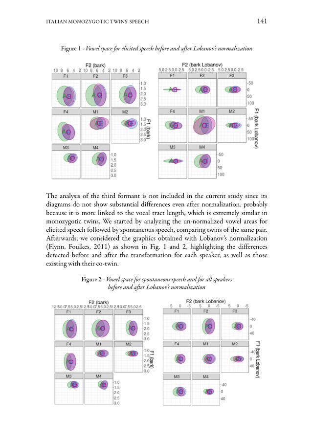
ITALIAN MONOZYGOTIC TWINS’ SPEECH 141
Figure 1 - Vowel space for elicited speech before and after Lobanov’s normalization
The analysis of the third formant is not included in the current study since its diagrams do not show substantial differences even after normalization, probably because it is more linked to the vocal tract length, which is extremely similar in monozygotic twins. We started by analyzing the un-normalized vowel areas for elicited speech followed by spontaneous speech, comparing twins of the same pair. Afterwards, we considered the graphics obtained with Lobanov’s normalization (Flynn, Foulkes, 2011) as shown in Fig. 1 and 2, highlighting the differences detected before and after the transformation for each speaker, as well as those existing with their co-twin.
Figure 2 - Vowel space for spontaneous speech and for all speakers before and after Lobanov’s normalization

142 ALICE ALBANESI, SONIA CENCESCHI, CHIARA MELUZZI, ALESSANDRO TRIVILINI
4.1 Analysis of un-normalized data
4.1.1 Comparison between twins belonging to the same pairWe compared the vowel space of each couple in controlled speech (sentences) considering values of F0 and un-normalized formants. We noticed a strong level of correspondence between the two siblings’ diagrams both in Hertz and Bark units (Traunmüller, 1990).
Each target vowel shows the same centre of gravity and a remarkably similar distribution of formants. As displayed in Fig. 3, the distributions of the two female pairs (F1-F2 and F3-F4) are pretty resembling.
Figure 3 - Female couples’ vowel space
Additionally, there is a larger distinction in the vowel space of /a/ and /o/ in the first male couple M1-M2 (wider distribution for M1), while the centre of gravity location is the same for both brothers. Indeed, an almost total correspondence is detected in the properties of /e/ (Fig. 5). Similarly, the other pair of twins M3-M4 reveals a slight difference in distributions and in the midpoint of /a/, a little higher in M3 (Fig. 4).
Figure 4 - Male couples’ vowel space
However, it must be noted that the same level of between-vowel-space dissimilarity could also be found comparing the speech of a single person recorded in disparate moments (e.g., different social context or emotional state).
Moreover, male speakers show an intra-pair difference in the vowel area distribution which is a little more evident than for female couples, but the sample is too small to allow further generalizations.

ITALIAN MONOZYGOTIC TWINS’ SPEECH 143
4.1.2 Comparison between elicited and spontaneous speech for the same speakerWhen considering values of F0 and un-normalized formants for spontaneous speech, each speaker exhibits a smaller vocal area than in elicited sentences. Moreover, the centres of gravity tend to overlap (Fig. 5). This will be the focus of interesting considerations we shall address later.
Figure 5 - Elicited and spontaneous speech for all pairs
4.1.3 Comparison between spontaneous speech of twins belonging to the same pairSpontaneous speech heightens the similarity between siblings of the same female couples (Fig. 6) with respect to the elicited form (Fig. 7).
Figure 6 - Spontaneous speech vowel space for female pairs

144 ALICE ALBANESI, SONIA CENCESCHI, CHIARA MELUZZI, ALESSANDRO TRIVILINI
Figure 7 - Elicited speech vowel space for female pairs
The same pattern was observed for male speakers, as shown in Fig. 8 and 9. However, compared to the other pairs, M3 and M4 display a slightly greater difference, even though still considered irrelevant.
Figure 8 - Spontaneous speech vowel space for male couples
Figure 9 - Elicited speech vowel space for male couples
4.2 Analysis of normalized data
In order to look for more significant results, we opted for a normalization of formants with Lobanov’s formula. According to many studies in sociophonetics (e.g., Van der Harst, 2011), this procedure is preferred, since it reduces the difference between formantic values due to physiological factors and preserves more information about sociolinguistic variants. It would underline the dichotomies coming from social and environmental influence, emotional perturbations, personality, and the context of discussion the individual is facing during the verbal production (Van der Harst, 2011; Adank, 2003). Although this normalization usually works better with huge corpora, we proceeded anyway to understand its possible usefulness in a forensic

ITALIAN MONOZYGOTIC TWINS’ SPEECH 145
context, where recordings are often short in duration, and speakers to be compared are quite always limited in number.
Confronting the vowel space of each person before and after Lobanov’s normalization, we observed that M1, F2 and M4 kept on being almost identical, unlike what happened to their co-twins whose acoustic representations were quite different. Only the pair F3-F4 did not undergo variations for both speakers (Fig. 10).
Figure 10 - Vowel space before and after Lobanov’s normalization
4.2.1 Comparison of co-twins’ normalized data in elicited speechBefore normalization, vowel areas looked remarkably similar between co-twins, but once the procedure was applied, substantial differences could be observed in 3 out of 4 pairs.
Comparing normalized data of twins belonging to the same couple (e.g., Fig. 11), we noticed that the second formant maintains a similar distribution between siblings for all vowels. According to empirical theories, the more stable frequency (F2) is less affected by factors unrelated to the individual’s physiology (Adank, 2003).
The first formant’s behaviour, on the other hand, is extremely different and enables a speaker discrimination; this would confirm the theory of Adank et al. (2004) in attributing to Lobanov’s normalization the ability to highlight non-physiological but sociolinguistic dichotomies. A comparison of these distributions also suggested that twins exploit different vowel spaces differently: one employs anteriority-posteriority, while the other exploits height.
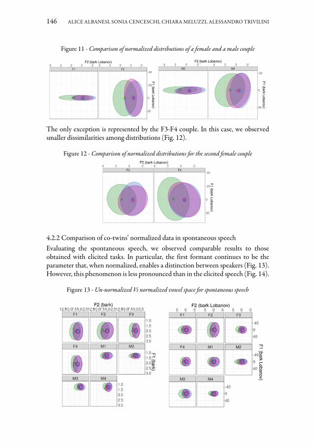
146 ALICE ALBANESI, SONIA CENCESCHI, CHIARA MELUZZI, ALESSANDRO TRIVILINI
Figure 11 - Comparison of normalized distributions of a female and a male couple
The only exception is represented by the F3-F4 couple. In this case, we observed smaller dissimilarities among distributions (Fig. 12).
Figure 12 - Comparison of normalized distributions for the second female couple
4.2.2 Comparison of co-twins’ normalized data in spontaneous speechEvaluating the spontaneous speech, we observed comparable results to those obtained with elicited tasks. In particular, the first formant continues to be the parameter that, when normalized, enables a distinction between speakers (Fig. 13). However, this phenomenon is less pronounced than in the elicited speech (Fig. 14).
Figure 13 - Un-normalized Vs normalized vowel space for spontaneous speech
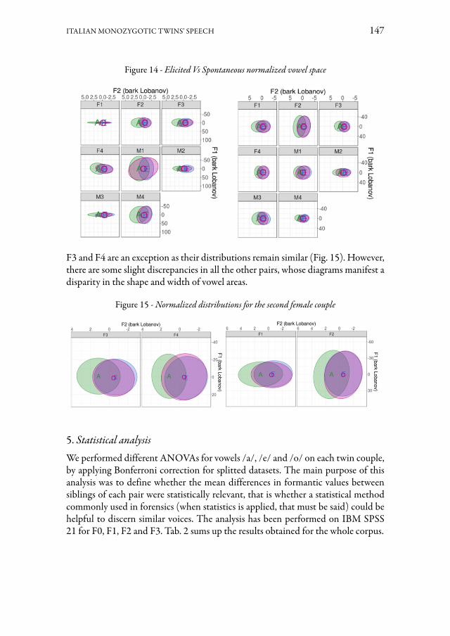
ITALIAN MONOZYGOTIC TWINS’ SPEECH 147
Figure 14 - Elicited Vs Spontaneous normalized vowel space
F3 and F4 are an exception as their distributions remain similar (Fig. 15). However, there are some slight discrepancies in all the other pairs, whose diagrams manifest a disparity in the shape and width of vowel areas.
Figure 15 - Normalized distributions for the second female couple
5. Statistical analysisWe performed different ANOVAs for vowels /a/, /e/ and /o/ on each twin couple, by applying Bonferroni correction for splitted datasets. The main purpose of this analysis was to define whether the mean differences in formantic values between siblings of each pair were statistically relevant, that is whether a statistical method commonly used in forensics (when statistics is applied, that must be said) could be helpful to discern similar voices. The analysis has been performed on IBM SPSS 21 for F0, F1, F2 and F3. Tab. 2 sums up the results obtained for the whole corpus.

148 ALICE ALBANESI, SONIA CENCESCHI, CHIARA MELUZZI, ALESSANDRO TRIVILINI
Table 2 - The results of the ANOVAs for vowel quality and group; significant correlations have been highlighted
Group 1 (F1-F2) Group 2 (F3-F4)/a/ /e/ /o/ /a/ /e/ /o/
F0 F(702)=1. 045; p=.307
F(642)=.599; p=.439
F(502)=1. 665; p=.198
F(802)=23. 363; p<.0001
F(664)=40. 196; p<.0001
F(520)=12. 432; p<.0001
F1 F(702)=1. 040; p=.308
F(642)=121. 103; p<.0001
F(502)=24. 206; p<.0001
F(802)=297. 087; p<.0001
F(664)=231. 543; p<.0001
F(520)=162. 941; p<.0001
F2 F(702)=2. 455; p=.118
F(642)=19. 349; p<.0001
F(502)=.549; p=.459
F(802)=.329; p=.566
F(664)=8. 750; p=.003
F(520)=1. 287; p=.257
F3 F(702)=59. 601; p<.0001
F(642)=10. 625; p<.0001
F(502)=25. 583; p<.0001
F(802)=116. 499; p<.0001
F(664)=229. 77; p<.0001
F(520)=93. 901; p<.0001
Group 3 (M1-M2) Group 4 (M3-M4)/a/ /e/ /o/ /a/ /e/ /o/
F0 F(835)=1. 872; p=.172
F(800)=2. 073; p=.150
F(746)=6. 084; p=.014
F(659)=17. 851; p<.0001
F(659)=21. 418; p<.0001
F(520)=10. 191, p<.0001
F1 F(835)=3. 019; p<.0001
F(800)=26. 631; p<.0001
F(746)=8. 407; p=.004
F(659)=10. 931; p<.0001
F(659)=.113; p=.737
F(520)=4. 80; p=.029
F2 F(835)=2. 361; p=.125
F(800)=2. 947; p=.086
F(746)=.998; p=.318
F(659)=29. 825; p<.0001
F(659)=11. 852; p<.0001
F(520)=.118; p=.731
F3 F(835)=137. 26; p<.0001
F(800)=75. 497; p<.0001
F(746)=29. 602; p<.0001
F(659)=.212; p=.645
F(659)=15. 473; p<.0001
F(520)=1. 081; p=.299
Data showed that the third formant seemed to be more sensitive in discriminating siblings, since the only exception is represented by the M3-M4 pair, where only vowel /e/ showed a significant difference between the two speakers. The second formant was relevant just for front vowels and for /e/ in particular, whereas the situation was more scattered for the first formant, as well as for the fundamental frequency. It also seemed that discrepancies highlighted for the first female pair (F1-F2) were in general less meaningful than in other pairs of our sample. The same could be said for the first male couple (group 3) when compared to the second one (group 4). However, the situation appears slightly different when we check dissimilarities by also dividing for speech task, which is elicited (Tab. 3) and spontaneous (Tab. 4) speech.
Table 3 - The results of the ANOVAs for vowel quality and group in elicited speech; significant correlations have been highlighted
Group 1 (F1-F2) Group 2 (F3-F4)/a/ /e/ /o/ /a/ /e/ /o/
F0 F(231)=1. 407; p=.237
F(256)=3. 574; p=.060
F(163)=1. 229; p=.269
F(291)=10. 023; p=.002
F(279)=7. 667; p=.006
F(215)=4. 683; p=.032
F1 F(231)=6. 602; p=.011
F(256)=3. 903; p=.049
F(163)=7. 451; p=.007
F(291)=46. 677; p<.001
F(279)=74. 465; p<.001
F(215)=39. 751; p<.001
F2 F(231)=.239; p=.626
F(256)=.184; p<.001
F(163)=.965; p=.327
F(291)=5. 275; p=.022
F(279)=5. 112; p=.025
F(215)=5. 899; p=.016
F3 F(231)=40. 228; p<.001
F(256)=.1. 478; p=.225
F(163)=23. 488; p<.001
F(291)=24. 151; p<.001
F(279)=67. 611; p=.001
F(215)=13. 539; p<.001
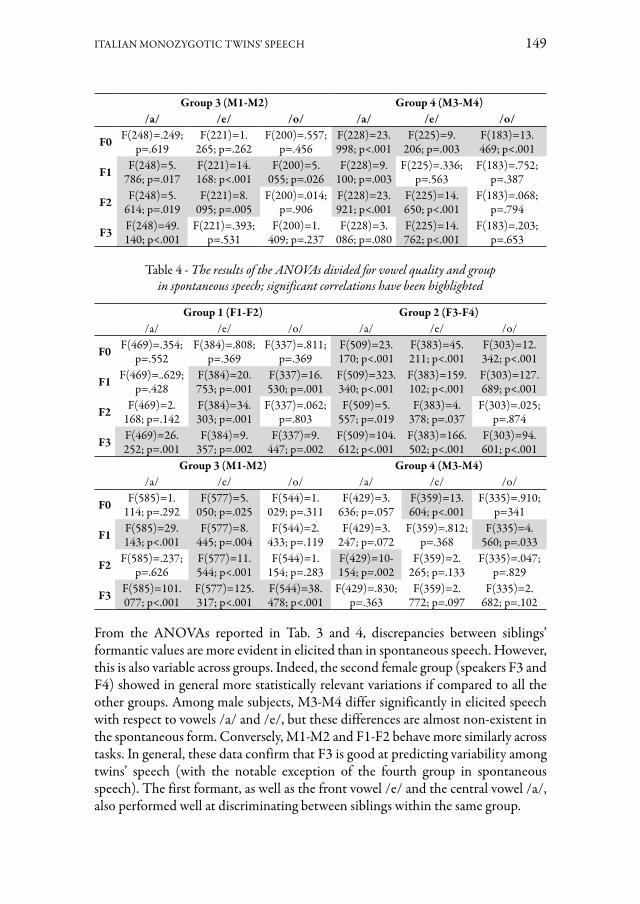
ITALIAN MONOZYGOTIC TWINS’ SPEECH 149
Group 3 (M1-M2) Group 4 (M3-M4)/a/ /e/ /o/ /a/ /e/ /o/
F0 F(248)=.249; p=.619
F(221)=1. 265; p=.262
F(200)=.557; p=.456
F(228)=23. 998; p<.001
F(225)=9. 206; p=.003
F(183)=13. 469; p<.001
F1 F(248)=5. 786; p=.017
F(221)=14. 168: p<.001
F(200)=5. 055; p=.026
F(228)=9. 100; p=.003
F(225)=.336; p=.563
F(183)=.752; p=.387
F2 F(248)=5. 614; p=.019
F(221)=8. 095; p=.005
F(200)=.014; p=.906
F(228)=23. 921; p<.001
F(225)=14. 650; p<.001
F(183)=.068; p=.794
F3 F(248)=49. 140; p<.001
F(221)=.393; p=.531
F(200)=1. 409; p=.237
F(228)=3. 086; p=.080
F(225)=14. 762; p<.001
F(183)=.203; p=.653
Table 4 - The results of the ANOVAs divided for vowel quality and group in spontaneous speech; significant correlations have been highlighted
Group 1 (F1-F2) Group 2 (F3-F4)/a/ /e/ /o/ /a/ /e/ /o/
F0 F(469)=.354; p=.552
F(384)=.808; p=.369
F(337)=.811; p=.369
F(509)=23. 170; p<.001
F(383)=45. 211; p<.001
F(303)=12. 342; p<.001
F1 F(469)=..629; p=.428
F(384)=20. 753; p=.001
F(337)=16. 530; p=.001
F(509)=323. 340; p<.001
F(383)=159. 102; p<.001
F(303)=127. 689; p<.001
F2 F(469)=2. 168; p=.142
F(384)=34. 303; p=.001
F(337)=.062; p=.803
F(509)=5. 557; p=.019
F(383)=4. 378; p=.037
F(303)=.025; p=.874
F3 F(469)=26. 252; p=.001
F(384)=9. 357; p=.002
F(337)=9. 447; p=.002
F(509)=104. 612; p<.001
F(383)=166. 502; p<.001
F(303)=94. 601; p<.001
Group 3 (M1-M2) Group 4 (M3-M4)/a/ /e/ /o/ /a/ /e/ /o/
F0 F(585)=1. 114; p=.292
F(577)=5. 050; p=.025
F(544)=1. 029; p=.311
F(429)=3. 636; p=.057
F(359)=13. 604; p<.001
F(335)=.910; p=341
F1 F(585)=29. 143; p<.001
F(577)=8. 445; p=.004
F(544)=2. 433; p=.119
F(429)=3. 247; p=.072
F(359)=.812; p=.368
F(335)=4. 560; p=.033
F2 F(585)=.237; p=.626
F(577)=11. 544; p<.001
F(544)=1. 154; p=.283
F(429)=10- 154; p=.002
F(359)=2. 265; p=.133
F(335)=.047; p=.829
F3 F(585)=101. 077; p<.001
F(577)=125. 317; p<.001
F(544)=38. 478; p<.001
F(429)=.830; p=.363
F(359)=2. 772; p=.097
F(335)=2. 682; p=.102
From the ANOVAs reported in Tab. 3 and 4, discrepancies between siblings’ formantic values are more evident in elicited than in spontaneous speech. However, this is also variable across groups. Indeed, the second female group (speakers F3 and F4) showed in general more statistically relevant variations if compared to all the other groups. Among male subjects, M3-M4 differ significantly in elicited speech with respect to vowels /a/ and /e/, but these differences are almost non-existent in the spontaneous form. Conversely, M1-M2 and F1-F2 behave more similarly across tasks. In general, these data confirm that F3 is good at predicting variability among twins’ speech (with the notable exception of the fourth group in spontaneous speech). The first formant, as well as the front vowel /e/ and the central vowel /a/, also performed well at discriminating between siblings within the same group.

150 ALICE ALBANESI, SONIA CENCESCHI, CHIARA MELUZZI, ALESSANDRO TRIVILINI
6. DiscussionTo discuss potential solutions for monozygotic twins’ acoustic distinction, we proceeded by synthesizing the obtained results and crossing them with social and context information:– F0 and F3 distributions were extremely similar for co-twins and did not undergo
major variations (especially if normalized); as for F0 this has been statistically confirmed, while for F3 the statistical analysis has shown its reliability as a quantitative cue for an intra-twin discrimination.
– Vowel spaces and distributions of the first two formants were extremely similar for co-twins within the same group.
– The only normalization that brings out evident differences between co-twins’ speech, for the first formant, is through Lobanov’s formula.
– Lobanov’s normalization seems to be more effective for elicited speech than for spontaneous speech, although in both cases it brings out variations between co-twins.
– The different discriminatory value of the tasks has also been confirmed by the statistical analysis, although it seems to be strongly group dependent (see below).
The most interesting parameter is therefore the first formant, when data have been subjected to Lobanov’s transformation. Assuming that Lobanov evidence could underline socio-phonetic differences related to the context of growth (Van der Harst, 2011; Adank, 2003), we tried to sketch some preliminary hypothesis and logical remarks based on the personal history of speakers.
The first and fourth couple (M1-M2; F3-F4) meet predictions and support this theory. In spite of living together and pursuing university degrees, the male twins embrace vastly different social circumstances, such as their university path, sports, employment and love lives.
In fact, M2 shows more stable formants, with a more contained extension of the vowel area linked to the lower F1 variation, while M1 presents opposite characteristics.
On the contrary, F3 and F4 have many things in common and lead similar lives. They live together, attend the same academic year, share a passion for the same sport they have been practicing together for years, and neither of them is romantically involved. The close similarity in social life matches with a strong resemblance in their vowel space.
However, when tested quantitatively, data from Tab. 3 and 4 revealed that F3 and F4, although visually very similar in terms of vowel space, displayed a statistically significant variability in the mean values of all formants (with the exception of the second formant of /o/ in spontaneous speech). This led to two distinct kinds of considerations: the first one concerns the impact of normalization procedures, and the second one focuses on the interaction between qualitative and quantitative analysis for forensic purposes (see 6.1).
As we have seen, compared to the other pairs in our study, F3-F4 twins were almost undistinguishable after Lobanov’s normalization. Instead, for both F1-F2 and M3-M4, even though the social context matched, Lobanov underlined some differences in their formants’ variability.

ITALIAN MONOZYGOTIC TWINS’ SPEECH 151
Hence, we concluded that Lobanov normalized results could be explained by considering speakers’ emotional sphere, which is influenced by their life background. Social conditions and life experiences of twins could be similar, but it does not imply (and it is unrealistic to think so) that their emotional responses and subjective characters are also aligned. In this scenario, twins may have a different emotional response to the elicited task (for instance, nervous or extroverted), resulting in different vowel areas with Lobanov’s formula.
Supporting this hypothesis, we noticed that subjects who were more nervous during the formulation of the 31 elicited sentences showed a greater variability of the first formant than their co-twin, who seemed to be calmer and more relaxed. For example:– The recording of the F2 female has been repeated several times, since her fear of
making mistakes induced her to a nervous laughter and frequent interruptions. Conversely, her sister, speaking in confidence with the technician (the first author), showed determination and firmness throughout the acquisition.
– M1 was asked to repeat the test, livening it up to sound less monotonous; therefore, the tension coming from the need to follow precise directions could have been a determining factor. His brother M2, on the other hand, adopted a less variable prosody, reciting the sentences with less emphasis and less marked prosodic variability; not having to meet specific requests, he seemed to be calmer and more relaxed as he was not subjected to pressure.
– This contrast between un-normalized and normalized vowel spaces was also found in the third pair, who presented less variable formantic values in M3 than in M4. As we acquired the audio samples through a telephone call, we were unable to assess the subjects’ state of mind, but it is plausible that they approached the task with a different emotional attitude, and that normalization accentuated their conflicting emotions.
– F3 and F4 speakers were apparently both noticeably quiet during the test, and marked differences in temperament could not be discerned. Since both of them have similar lives and social relationships, it is possible that normalization was not able to differentiate them at an emotional level.
6.1 Application in Forensics
The potential impact for this (extremely preliminary) study in the forensic field is two-fold. As addressed in the previous section, there was not always a straight correspondence between the results of the visual (qualitative) analysis of vowel space and the statistical analysis as performed on different formants. The main distinction has been highlighted for the second female pair (F3-F4), whose vowels’ distribution appeared similar, especially after Lobanov’s transformation, but in the statistical research their formants’ values were the most different among the groups of our study. This would suggest a need to be cautious when preferring one analysis to the other. Due to the limited amount of data to investigate, qualitative examination is sometimes preferred in forensics, especially since its results are more understandable by relevant

152 ALICE ALBANESI, SONIA CENCESCHI, CHIARA MELUZZI, ALESSANDRO TRIVILINI
third parties (e.g., judges and lawyers). However, it remains to be investigated whether formants’ differences highlighted by the quantitative analysis have a real phonetic counterpart, which is whether these dichotomies are perceivable by listeners. A perceptual experiment, carefully designed and balanced, may help clarify these (only apparent) contradictions between qualitative and quantitative outcomes.
Furthermore, this work suggests a possible starting point for cases of uncertain attribution through the recording of a phonic test for each twin. Performing a test that “puts under emotional pressure” or causes different speech moods in the two speakers could allow to enhance differences in vowel spaces and in the first formant’s distribution with Lobanov’s normalization.
As an example, in the Italian authority, phonic tests are normally recorded by asking suspected people to perform a spontaneous speech task within some lists of target words or sentences. On the contrary, if the conclusions derived from the present examination will be validated in further studies, elicited/controlled speech will be more important than the spontaneous one for twins’ discrimination.
We state that considerations exposed so far emerged for the first time while performing the present research, therefore it is still not possible to know their value. For this reason, further work will involve a greater number of twin pairs, and we intend to integrate our analysis with other acoustic parameters such as jitter, shimmer and MFCCs. Moreover, vowel observations will be refined in order to study in detail the proximity to certain consonants and their dynamic behaviour (over 7-time steps). A parallel investigation concerns the perceptual aspect: once the analysis of the corpus is completed, a perceptual test will be prepared to understand whether the hearing system validates the results. The hope is that this preliminary outcome could lead to innovative solutions for monozygotic twins’ distinction, but also to perform in-depth analysis on sociophonetic variability.
7. ConclusionsDrawing a preliminary conclusion, the fundamental frequency, the third formant and the first two un-normalized formants of our monozygotic twins have too similar values and do not allow a visual discrimination (both in Hz and Bark). Despite the work being focused on a limited number of speakers and sentences, it is entirely possible that this finding could be extended to any monozygotic pair living in similar social conditions and sharing past backgrounds. Lobanov’s formula seems to be a suitable method to be explored, especially for what concerns elicited speech or, better, recording in stressful conditions.
Lobanov’s normalization of spontaneous speech formants always highlights discrepancies between speakers of each pair, but less than in the elicited form. However, this provides a valid contribution supporting the hypothesis that Lobanov’s transformation could highlight emotional and attitudinal differences in siblings with the same genetic makeup and aligned life experiences. In the spontaneous speech task, the speaker was free to express himself without interruptions by the

ITALIAN MONOZYGOTIC TWINS’ SPEECH 153
technician. This suggests that people found themselves in a more comfortable situation, with the consequence that different emotional characters did not come to light. Moreover, we must also take into account that spontaneous speech could emphasize more the phenomenon of accommodation, which surely occurs in subjects who are in daily contact and who live in the same families, just like our speakers. Then, accommodation could be mitigated by the executive restrictions of the elicited task, where emotions seem to predominate.
Bibliography
Adank, P., Smits R. & van Hout, R. (2004). A comparison of vowel normalization procedures for language variation research. In Journal of the Acoustical Society of America, 116(5), 3099-3107.Berry, M., Brown, S. (2019). Acting in action: Prosodic Analysis of Character Portrayal during Acting. In Journal of Experimental Psychology, 48(8), 1407-1425.Byrne, C., & Foulkes, P. (2004). The ‘mobile phone effect’ on vowel formants. In The International Journal of Speech, Language and the Law, 11(1), 83-102.Boersma, P., Weenink, D. (2019). PRAAT: doing phonetics by computer [Computer program]Version 6.0.52, retrieved from http://www.PRAAT.org/Cenceschi, S., Meluzzi, C. & Trivilini, A. (2021). The Variability of Vowels’ Formants in Forensic Speech. In IEEE Instrumentation & Measurement Magazine, 24(1), 38-41.Cenceschi, S., Meluzzi, C. & Nese, N. (2020). Speaker’s identification across recording modalities: a preliminary phonetic experiment. In Romito L. (Ed.). Language change under contact conditions: acquisitional contexts, languages, dialects and minorities in italy and around the world, Studi AISV 7. Milano: Officinaventuno, 407-426.Cenceschi, S., Sbattella, L. & Tedesco, R. (2018). Verso il riconoscimento automatico della prosodia. In Bertini C., Celata C., Lenoci G., Meluzzi C & Ricci I. (Eds.). Social and biological factors in speech variation, Studi AISV 3. Milano: Officinaventuno, 433-440.Cheng, E., & Burnett, I.S. (2011). On the effect of AMR and AMR-WB GSM compression on overlapped speech for forensic analysis. In Proceeding of the 2011 IEEE International Conference on Acoustics, Speech and Signal Processing (ICASSP) 1872-1875.Cresti, E., Moneglia, M. (Eds.). (2005). C-oral-rom: integrated reference corpora for spoken romance languages. Amsterdam: John Benjamins publishing.Falcone, M., Gallo, A. (1996). The “SIVA” speech database for speaker verification: description and evaluation. In Bunnell, H.T., Idsardi, W. (Eds.) (1996). Proceeding of Fourth International Conference on Spoken Language Processing, Philadelphia, USA, 3-6 October 1996, 1902-1905.Fernández, E.S.S. (2013). A phonetic corpus of Spanish male twins and siblings: Corpus design and forensic application. In Procedia-Social and Behavioral Sciences, 95, 59-67.Frota, S., Prieto, P. (Eds.). (2015). Intonation in Romance. Oxford: Oxford University Press.

154 ALICE ALBANESI, SONIA CENCESCHI, CHIARA MELUZZI, ALESSANDRO TRIVILINI
Gahl, S., Baayen, R.H. (2019). Twenty-eight years of vowels: Tracking phonetic variation through young to middle age adulthood. In Journal of Phonetics, 74, 42-54.Giannini, A. (1989). Test acustico-percettivo su voci di gemelli. In Proceedings of the xvii convegno nazionale AIA, Parma, Italy, 12-14 april 1989, 427-432.Giannini, A., Pettorino M. (1992) La fonetica sperimentale. Napoli: Liguori, 197.Gedda, L., Bianchi, A. & Bianchi-Neroni, L. (1958). La Voce dei Gemelli—I. Prova di identificazione intrageminale della voce in 104 coppie (58 MZ e 46 DZ). In Acta geneticae medicae et gemellologiae: twin research, 4(2), 121-130.Gonzalez, J., Cervera, T. & Llau, M.J. (2003). Acoustic analysis of pathological voices compressed with MPEG system. In Journal of voice, 17(2), 126-139.Heeringa, W., Van de Velde, H. (2017). Visible Vowels: A Tool for the Visualization of Vowel Variation. In International Speech Communication Association (ISCA) (Ed.) (2017). Proceedings of INTERSPEECH 2017, Stockholm, August 20–24, 4034-4035.Jensen, K. (2002). The timbre model. In Journal of the Acoustical Society of America, 112(5), 2238-2238.Johnson, K., Azara, M. (2000). The perception of personal identity in speech: evidence from the perception of twins’ speech. Unpublished manuscript.Kader, F., Ghai, M. & Olaniran, A.O. (2020). Characterization of DNA methylation-based markers for human body fluid identification in forensics: a critical review. In International journal of legal medicine, 134(1), 1-20.Künzel, H.J. (2001). Beware of the ‘telephone effect’: the influence of telephone transmission on the measurement of formant frequencies. In Forensic Linguistics, 8(1): 80–99.Künzel, H.J. (2002) ‘Rejoinder to Francis Nolan’s “The ‘telephone effect’ on formants: a response”’, Forensic Linguistics, 9(2): 83–6.Künzel, H.J. (2010). Automatic speaker recognition of identical twins. In International Journal of Speech, Language, and the Law, 17(2), 251-277.Loakes, D. (2008). A forensic phonetic investigation into the speech patterns of identical and non-identical twins. In International journal of speech, language, and the law, 15(1), 97-100.Lobanov, B.M. (1971). Classification of Russian Vowels Spoken by Different Speakers. In Journal of the Acoustical Society of America, 49(2), 606-608.Nolan, F., Oh, T. (1996). Identical twins, different voices. In International Journal of Speech, Language, and the Law, 3(1), 39-49.Planterose Jiménez, B., Liu, F., Caliebe, A., Montiel González, D., Bell, J.T., Kayser, M. & Vidaki, A. (2021). Equivalent DNA methylation variation between monozygotic co-twins and unrelated individuals reveals universal epigenetic inter-individual dissimilarity. In Genome Biology, 22(18): doi:10.1186/s13059-020-02223-9Prieto, P., Borràs-Comes, J. & Roseano, P. (coords.) (2010-2014). Interactive atlas of romance intonation, retrieved from http://prosodia.upf.edu/iari/.Rietveld, A.C.M., van Heuven, V.J. (2009). Algemene fonetiek. Bussum: Uitgeverij Coutinho.Rhodes, R.W. (2012). Assessing the strength of non-contemporaneous forensic speech evidence, PhD dissertation, University of York.

ITALIAN MONOZYGOTIC TWINS’ SPEECH 155
San Segundo, E., Künzel, H. (2015). Automatic speaker recognition of Spanish siblings:(monozygotic and dizygotic) twins and non-twin brothers. In Loquens, 2(2), e021-e021.San Segundo, E., Tsanas, A. & Gómez-Vilda, P. (2017). Euclidean distances as measures of speaker similarity including identical twin pairs: a forensic investigation using source and filter voice characteristics. In Forensic Science International, 270, 25-38.Sebastian, S. (2013). An investigation into the voice of identical twins. In Otolaryngology online journal, 3(2), 9-15.Van Braak, P., Heeren, W.F.L. (2015). “Who’s calling, please?” Is there speaker-specific information in twins’ vowels?. In 24th Annual Conference of the International Association for Forensic Phonetics and Acoustics, Leiden, Netherlands, 7-10 July 2015, conference presentation.Van, W.G., Vercammen, j. & Debruyne, F. (2001). Voice similarity in identical twins. In Acta oto-rhino-laryngologica belgica, 55(1), 49-55.Vidaki, A., López, C.D., Carnero-Montoro, E., Ralf, A., Ward, K., Spector, T. & Kayser, M. (2017). Epigenetic discrimination of identical twins from blood under the forensic scenario. In Forensic Science International: Genetics, 31, 67-80.Traunmüller, H. (1981). Perceptual dimension of openness in vowels. In The Journal of the Acoustical Society of America, 69(5), 1465-1475.Zuo, D., Mok, P.P.K. (2015). Formant dynamics of bilingual identical twins. In Journal of phonetics, 52, 1-12.


DOI: 10.17469/O2108AISV000009
CAROLINA LINS MACHADO
A cross-linguistic study of between-speaker variability in intensity dynamics in L1 and L2 spontaneous speech
Dynamic aspects of the amplitude envelope appear to reflect speaker-specific information. Intensity dynamics characterized as the temporal displacement of acoustic energy associated to articulatory mouth opening (positive) and closing (negative) gestures was able to explain between-speaker variability in read productions of native speakers of Zürich German. This study examines positive and negative intensity dynamics in spontaneous speech produced by Dutch speakers using their native language and English. Acoustic analysis of informal monologues was performed to examine between-speaker variability. Negative dynamics explained a larger quantity of inter-speaker variability, strengthening the idea of a lesser prosodic control over the mouth closing movement. Furthermore, there was a significant effect of language on intensity dynamics. These findings suggest that speaker-specific information may still be embedded in these time-bound measures despite the language in use.
Keywords: inter-speaker, cross-linguistic, variability, intensity, dynamics.
1. IntroductionSpeech is a dynamic process involving the articulators in our vocal tract that give rise to phonetic sounds. These sounds carry meanings that are specific to each language, making possible the communication of people sharing the same linguistic background. Other than meaning, speech also contains information related to the speaker (Coulthard, Johnson & Wright, 2016: 136). This extra-linguistic information, considered to be a by-product of speaker-specific biomechanical characteristics (Perrier, Winkler, 2015), is extremely valuable in the field of forensic phonetics, where, among other tasks, speaker comparison is often employed.
Speaker comparisons involve comparing speech samples of an unknown speaker to samples of a known speaker to determine whether the unknown samples may belong to the known speaker or to a different speaker. This task can be described as an auditory-acoustic analysis where an experienced forensic phonetician performs an aural-perceptual investigation and examines the acoustic features of the speech signal (Rose, 2002; Coulthard et al., 2016). Among these acoustic features, measures of fundamental frequency (Rose, 2002; Gold, French, 2011) and vowel formants (Goldstein, 1976; McDougall, 2007; He, Zhang & Dellwo, 2019) are some of the most studied parameters, which have been extensively employed in speaker comparisons. However, there are still understudied acoustic features containing significant speaker-specific information, one of such being intensity dynamics.

158 CAROLINA LINS MACHADO
Intensity by itself is not considered a useful discriminative feature (other than in the context of formants) because of how easily it can be distorted (Hollien, 1990: 198). However, considering the temporal organization of intensity provides a different approach to the use of this acoustic feature. Intensity dynamics is an aspect of speech rhythm, which has been considered a useful parameter for speaker discrimination (Gold, French, 2011: 302). Therefore, investigating inter-speaker variation in intensity dynamics may further contribute to understanding this rhythmic aspect of speech and provide insight into whether it could be useful in forensic applications.
Figure 1 - The upper plot contains an oscillogram of the Dutch word “student” in teal and its amplitude envelope (superimposed in red). The lower plot illustrates
the intensity curve, its peak (IP) and valley (IV) values, and time points associated with them (tP and tV). These plots are based on the description of positive
and negative dynamics by He, Dellwo (2017)
Intensity dynamics can be understood as the rate of energy increase and decrease in the acoustic signal and is calculated by analyzing the amplitude envelope of the acoustic signal (He, Dellwo, 2017). This concept is demonstrated in Figure 1. In the disyllabic Dutch word “student” there are two syllabic peaks, i.e. places with large amounts of energy in a syllable, and one place with relative low amounts of energy between them, i.e. a valley. IP are peak points where intensity reaches its maximum value, and IV is the point where intensity is at its minimal relative to these peaks. Positive dynamics is the rate of increase in intensity from a valley (IV) to its right adjacent peak (IP). Negative dynamics is rate of decrease in intensity between a peak (IP) and the next valley point in time (IV). In the figure above, negative dynamics

A CROSS-LINGUISTIC STUDY OF BETWEEN-SPEAKER VARIABILITY 159
is demonstrated in the intensity curve (lower plot) by the red secant line IPIV and positive dynamics by the secant line IVIP.
Changes in intensity are mainly a result of subglottal pressure variation, although both glottal and supra-glottal regions also affect intensity (Fry, 1979; Stevens, 2000). Regarding the supra-glottal region, it has been proposed and empirically demonstrated that the size of mouth opening is one of the factors determining the overall intensity of the speech stream (Summerfield, 1992; Chandrasekaran, Friston, Trubanova, Stillittano, Caplier & Ghazanfar, 2009; Titze, Palaparthi, 2018). Chandrasekaran et al. (2009) found evidence for the relationship between intensity and the articulatory movements responsible for mouth opening and closing gestures. This study established that the amplitude envelope is closely related to the time course of the opening and closing mouth gestures in both read and spontaneous speech samples in two languages, English and French. Furthermore, the authors observed a significant amount of intra- and inter-speaker variability in the temporal patterns of both mouth gestures and the amplitude envelope (Chandrasekaran et al., 2009: 5). Their results were later supported by He, Dellwo (2017), who suggested that inter-speaker variability in the temporal organization of intensity contours of Zürich German speakers may reveal the influence of speaker-specific neurophysiological characteristic over mouth opening and closing movements.
Speaker-specific effects on dynamic acoustic features reflect behavioral variation (Kitamura, Akagi, 2007), i.e. the idiosyncratic way a person operates their articulators to produce speech. Speech articulation is so particular to a speaker that even twins, who have the same anatomical structures allowing them to produce the same canonical phonetic segments, show variation in their production of acoustic dynamic features (Zuo, Mok, 2015). Interestingly, He, Dellwo (2017) observed that in read speech productions negative intensity dynamics showed more between-speaker variability than positive dynamics. They interpreted the lesser variability in positive dynamics as a result of greater prosodic control over the mouth opening gesture during speech production, suggesting that this gesture may exhibit less speaker-specific information due to its function. The authors argued that positive dynamics ask for a more controlled mouth opening to reach the presumed articulatory state of a phonetic segment (phonetic target). Mouth closing gestures on the other hand, were believed to be realized under less prosodic control. That is, once the phonetic target has been reached, speakers may reduce control over this articulatory gesture, which in turn can result in movements exhibiting speakers’ behavioral and biological characteristics.
The same result was demonstrated in an earlier study, where De Nil, Abbs (1991) found a wide variety of mouth closing sequencies involving the lower lip, upper lip and jaw in the production of the same utterance by different speakers. Besides the different closing sequencies, they also noticed that some patterns were used more frequently by some speakers than by others. The fact that each of these articulators present a particular morphological structure (Perrier, Winkler, 2015) and are employed differently between-speakers helps understanding the variation found in He, Dellwo’s (2017) results. Overall, their study offered a significant contribution
→→

160 CAROLINA LINS MACHADO
to forensic phonetics, providing, as previously mentioned, an additional facet of speech rhythm. However, although a seemingly promising parameter, inter-speaker differences in intensity dynamics should also be studied under other conditions for a better understanding of this feature. Therefore, generalizations and replications in other languages and speech styles are necessary.
Speech production of native and non-native languages show similarities and differences. The underlying mechanisms of speech production in first (L1) and second (L2) languages share similarities related mainly to the mechanical apparatus used during speech production, which is theoretically the same for every healthy speaker (Hixon, Weismer & Hoit, 2020; Marchal, 2009). Differences in L1 and L2 productions are found in other complex mechanical and cognitive actions taking place before and during speech articulation, which are believed to be influenced by language-specific characteristics (Flege, 1995; Best, Tyler, 2006; Escudero, 2009). Although speech is perceived as a highly automatic undertaking in the L1, this is far from true, since, before words come out of our mouths, an utterance needs to be planned and structured (Levelt, 1989). The same is true for the L2, with added constraints related to the speaker’s knowledge of this language, and effects stemming, for instance, from the L1 phonology (Kormos, 2006).
Similar to differences owed to language specific constraints are differences across speaking styles. It has been proposed that spontaneous speech contains exclusive phonetic patterns setting it apart from other styles, such as read speech (Simpson, 2013). These patterns may be a result of the communicative situation a speaker is in, involving different factors that influence speech articulation and the resulting acoustic signal (Simpson, 2013: 163). For example, while reading a passage, speakers tend to focus more on the vocalization of the utterance, since there is no need to formulate the message being delivered because it is already given in the text. Contrariwise, when people are talking, information is in the foreground and attentional resources are being divided between the formulation of the content and the act of vocalization.
Together, differences between languages and speaking styles along with the singular way speakers use their anatomically distinctive speech apparatus have a significant effect on the acoustic features of speech. Therefore, this study seeks to fill the gap in our current knowledge by investigating whether intensity dynamics also vary between speakers in spontaneous productions in their L1 and in an L2, and whether there is an influence of language over this feature. More specifically, this study seeks to answer the following questions:– RQ1: Do measures of intensity dynamics vary between native Dutch speakers?– RQ2: Is this between-speaker variability also present when these speakers use
English, a second language they are proficient in?– RQ3: Does language influence intensity dynamics?Regarding RQ1 and RQ2 I hypothesize that between-speaker variability in intensity dynamics will be evident despite the language spoken by the speaker, since this variability is a result of speaker-specific characteristics (He, Dellwo, 2017), meaning

A CROSS-LINGUISTIC STUDY OF BETWEEN-SPEAKER VARIABILITY 161
that productions of native Dutch speakers will vary between speakers in the L1 and in the L2 English. Regarding RQ3, I hypothesize that there will be an effect of language on intensity dynamics, analogous to previous studies in speech dynamics (Schwartz, Kazmierski, 2019).
2. Methodology2.1 Corpus
The D-LUCEA corpus was used in this study (see Orr, Quené, 2017 for further details), from which 51 female native Dutch speakers (age range of approx. 17–26 years with no reported speech and hearing disorders) were selected based on the quality of their recording. Participants were recruited at University College Utrecht (UCU) and they reported their proficiency in English by providing the results of a formal proficiency exam, which is an entry requirement for this language at UCU with the minimum level of proficiency similar to B1 according to the Common European Framework of Reference for Languages. Additionally, information regarding their language background was collected via a questionnaire where speakers had to report their age of acquisition and degree of exposure to the language (Orr, Quené, Beek, Diefenbach, Leeuwen & Huijbregts, 2011). Each participant was simultaneously recorded via eight microphones in a quiet furnished office with at least one facilitator seated at the opposite side from the speaker (Orr, Quené, 2017). For this study the selected recordings were the ones captured by the microphone closest to the speaker (Sennheiser Headset HSP 2ew; 44.1 kHz; 16 bit), since this microphone had little variation in the distance between the microphone and the speaker’s mouth.
From a total of six performed speaking tasks, two two-minute-long prepared informal monologues on a free topic in English (L2) and in Dutch (L1) were selected for this study. Most speakers repeated the same monologue in both languages; however, some of them simply continued the monologue started in one language. These monologues were manually annotated by two annotators and checked by a third annotator at four levels: Language spoken, speech type, speech and silence intervals, and an orthographic transcription of the utterances. Additionally, two more levels were annotated by the author; namely, stretches of fluent uninterrupted speech, which were manually selected to ensure precision, followed by an automatic segmentation of these stretches into smaller chunks. The nature of these chunks is described in the following section.
2.2 Data Preparation
Prior to speech chunking, audio signals containing only the prepared monologues in the L1 and the L2 were automatically extracted and stored as separate audio files,

162 CAROLINA LINS MACHADO
to reduce lag during subsequent steps and to normalize amplitude by language1. The chunking of the spontaneous speech data was achieved by obtaining uninterrupted speech segments between 1.4 s and 1.6 s following Tilsen, Arvaniti (2013). This method reduces any variation that may be caused by differences in speech tempo and resolves the issue of time normalization, since chunk durations are uniformly distributed around 1.5 seconds with a ± 100 ms variation from this value (Tilsen, Arvaniti, 2013: 629).
The resulting speech signals were then prepared in Praat (Boersma, Weenink, 2021), following the initial stages of He, Dellwo’s (2017) methodology. First, the DC bias was removed by subtracting the mean amplitude from the signal; then a higher-sampled amplitude envelope was created by low-pass filtering the full-wave rectified speech signal at 10 Hz [Hann filter, roll-off = 6 dB/octave]. Next, an intensity object was created in Praat (using the command To Intensity..., with Minimum pitch = 100 Hz; Time step = 0.0 s; Subtract mean = True). This command squares and windows the signal before creating the intensity object (Kaiser-Bessel window: 𝛽 = 20; side lobe attenuation ≅ –190 dB; length: 32 ms). This series of signal manipulations results in the amplitude envelope of each signal and its intensity object containing intensity point values in time.
Next, the values in the intensity curve were linearly normalized within the range [0.01, 1] using the formula:
(1)
Where I´( f ) and I( f ) refer to the normalized and original intensity value at frame index f; max and min refer to the maximum and minimum values of the original intensity curve, and 1 and 0.01 are the new maximum and minimum values of I´( f ). This procedure is analogous to the one employed by He et al. (2019) for the normalization of the first formant (F1). The authors proposed that the normalized curve maintains only information related to the trajectory of the (F1) curve that can be associated to speaker-specific articulatory gestures (He et al., 2019: 210).
Finally, the detection of intensity peaks and valleys was done semi-automatically. Instead of placing these points between pre-established syllable boundaries, an algorithm was created to automatically detect potential peak and valley points by surveying the amplitude envelope. After iterating through all points in the envelope collecting their intensity values in time, the algorithm determines if a point is a syllabic peak or valley by comparing successive intensity values. If the next value is larger than the current, the previous point is stored as a valley. Similarly, if the successive value is smaller than the previous point is stored as a peak. Next, all prospective pairs of peak and valley points are checked against each other. If their
1 Normalizing the L1 and L2 data separately ensures that, for each language sample, no cross-linguistic influence would affect the analyses of the extracted measures of intensity dynamics.

A CROSS-LINGUISTIC STUDY OF BETWEEN-SPEAKER VARIABILITY 163
difference is larger than a predetermined threshold (min 5 dB), they are considered as valid syllabic peaks or valleys. The output of this process is a series of intensity values in time of peak and valley points of each syllable in a continuous stretch of speech. These values were used in the automatic placement of peak and valley demarcation points in the intensity contour. These points were then manually checked to ensure correct placement.
2.3 Data Extraction
The intensity values of peaks and valleys were obtained at each of the demarcation points from the intensity curve using cubic interpolation, offering true continuity between the motion trajectories that pass through each peak and valley point. Next, positive dynamics (𝜈I[+]) were computed by calculating the rate of intensity increased from a valley to its succeeding peak as follows:
(2)
Where IP and IV refer to the intensity values of the peak tP and valley tV points. Similarly, negative dynamics (𝜈I[–]) were measured by calculating the rate of intensity decrease from a peak to its right-adjacent valley as shown in (3):
(3)
Here the intensity values taken are absolute, since only the magnitude of the signal is of interest for the analyses (He, Dellwo, 2017: 490).
The distributions of positive and negative dynamics in a chunk of spontaneous speech were obtained by calculating the mean, standard deviation and Pairwise Variability Index, or PVI (Grabe, Low, 2002), of both types of dynamics from speakers’ positive and negative slopes by language (min = 167, max = 586). The mean and standard deviation of each dynamic type display the central tendency and the overall dispersion of a speaker’s intensity dynamics, respectively. The PVI conveys the amount of variability between successive syllables by computing and averaging the difference in duration between sequential intervals in an utterance (Grabe, Low, 2002). Following He, Dellwo’s (2017) notation of these measures, mean_𝜈I[–], stdev_𝜈I[–], and pvi_𝜈I[–] refer to negative dynamics and mean_𝜈I[+], stdev_𝜈I[+], and pvi_𝜈I[+] to positive dynamics. These measures were stored per chunk per speaker in separate data subsets corresponding to language spoken; namely, English (EN) and Dutch (NL).

164 CAROLINA LINS MACHADO
2.3 Statistical Analyses
According to He, Dellwo (2017) positive and negative measures may encode different types of information, which could be established if they are separated into two independent factors (He, Dellwo, 2017: 491). Therefore, factor analysis (FA) was employed on all measures of intensity dynamics in both language subsets to test whether positive and negative dynamics formed two independent categories (extraction method = principal components, eigenvalues ≧ 1; rotation method = Varimax with Kaiser normalization). Following, a multinomial logistic regression (MLR) was employed to assess how much inter-speaker variability is explained by the positive and negative dynamics. In this regression analysis, the measures of intensity dynamics were set as the numeric predictor variables and speaker as the nominal response variable.
Next, linear discriminant analysis (LDA) was employed to assess how well speakers can be discriminated based on positive and negative measures of intensity dynamics. The two types of dynamics were used as predictors in two separate analyses, one containing only positive measures and another containing only negative ones. In these analyses positive and negative measures are used as predictors, and speaker as the grouping variable (range = 1 to 51; within-group correlations with Fisher’s coefficient; prior probability from group sizes; leave-one-out cross-validation). Post-hoc analyses were carried out with each individual measure of both types of dynamics to assess which of these measures were better predictors of class.
Subsequently, the effect of language on speakers’ intensity dynamics was measured employing linear mixed-effects models (LME). In each model, built in a forward stepwise approach, one measure of intensity dynamics was assigned as the response variable, language as the main binary dummy fixed factor (0 = Dutch, 1 = English), and speaker as the random factor with by-language slopes (Bonferroni correction a posteriori). Assigning speakers as a random factor in the model increases the likelihood that a possible effect of language in the variation of these measures is genuine and can be generalized to all individuals fitting the sampling population (Walker, 2013: 454). These models were fitted in R (R Core Team, 2020) using the nlme package (Pinheiro, Bates, DebRoy & Sarkar, 2020) and using restricted maximum likelihood. Model selection was based on the best statistically significant model; in case of no significance in model fitness for a particular variable, the one with the lowest Log-likelihood value was selected.
3. ResultsTable 1 provides a statistical description of the measures of intensity dynamics in both language subsets (NNL = 1,843 and NEN = 1,633). The U-test (Wilcoxon rank-sum test) for central tendency suggests that the center of each measure of intensity dynamics differs significantly between both languages. At first glance, stdev_𝜈I[-] shows relatively low dispersion in both language subsets compared to the other measures. Conversely, pvi_𝜈I[–] shows the highest overall dispersion in L1 Dutch.

A CROSS-LINGUISTIC STUDY OF BETWEEN-SPEAKER VARIABILITY 165
Although means and standard deviations are given for the sake of completeness, a better overview of the central tendency and dispersion of each measure of positive and negative dynamics can be seen in the values of medians and interquartile ranges (IQRs), since there are valid outliers present in the data which do affect the two former statistical descriptors.
Table 1 - Means, standard deviations (SD), medians and IQRs for each measure of intensity dynamics by language. W indicates the result for the U-test for each measure of intensity
dynamics. Significance values as follows: ** p < 0.01; *** p < 0.001
L1 Dutch L2 English
Mean (SD) Median IQR Mean (SD) Median IQR W
mean_𝑣I[+] 4.25 (1.22) 4.19 1.59 4.12 (1.30) 4.03 1.76 1596146**
stdev_𝑣I[+] 2.18 ( .85) 2.13 1.15 2.11 ( .94) 2.01 1.24 1598605**
pvi_𝑣I[+] 6.33 (1.67) 6.21 1.97 5.65 (1.42) 5.61 1.80 1850840***
mean_𝑣I[–] 3.23 ( .89) 3.18 1.23 3.05 ( .90) 3.00 1.27 1680520***
stdev_𝑣I[–] 1.61 ( .68) 1.55 .96 1.54 ( .69) 1.48 .94 1595413**
pvi_𝑣I[–] 6.27 (1.73) 6.08 2.02 5.55 (1.39) 5.56 1.80 1867871***
3.1 Factor Analysis
For the Dutch subset the Kaiser-Meyer-Olkin (KMO) measure of sampling adequacy (KMO = .513 > .5) and the Barlett’s sphericity test (𝜒2 = 4666.932, p < .0005) indicated that the data was suitable for factor analysis. The same was true for the English subset (KMO = .533 > .5; 𝜒2 = 3422.131, p < .0005).
The results on Table 2 show that two factors were extracted for the L2 English subset. Factor 1 includes all measures of negative intensity dynamics while Factor 2 includes all measures of positive dynamics. This outcome suggests that there is orthogonality between the measures of positive and negative dynamics, since they were classified into different factors. For the L1 subset these results were partially similar. While all measures of negative dynamics were classified into one factor, an additional measure of positive dynamics, pvi_𝜈I[+], was classified into the same factor (Factor 1). The remaining two positive measures were classified into a different factor (Factor 2). The reason why pvi_𝜈I[+] was classified alongside the measures of negative dynamics for this subset may lie in the very strong positive correlation (r = .80) between both positive and negative PVI measures.

166 CAROLINA LINS MACHADO
Table 2 - Factor loadings matrix after Varimax rotation. Absolute values under the threshold (.40) were suppressed from the table. The shaded cells indicate the highest loading values
that classify a measure into a particular factor
L1 Dutch L2 EnglishFactor Loadings Factor Loadings
Factor 1 Factor 2 Factor 1 Factor2mean_𝑣I[–] .79 .83stdev_𝑣I[–] .79 –.72 .86 –.49
pvi_𝑣I[–] .70 .57mean_𝑣I[+] .82 .81stdev_𝑣I[+] .90 .88
pvi_𝑣I[+] .66 .43 .59Eigenvalue 2.54 1.35 2.51 1.37
% of variance 42.30 22.57 41.86 22.88
3.2 Multinomial Logistic Regression
The results of the regression analysis (Table 3) show how much inter-speaker variability was explained by each measure of intensity dynamics. For the models concerning the L1 subset, 48% of between-speaker variability was explained by the combined positive measures and 52% by the combined negative measures. Similarly, in the L2 subset 49% of this variability was explained by the combined positive measures, and 51% by the combined negative measures. Among the negative measures, stdev_𝜈I[–] seems to explain most variability in both subsets (Dutch = 28.95%, English = 18.35%); among the positive measures pvi_𝜈I[+] seems to better explain this variability in the L2 (18.30%), and stdev_𝜈I[+] in the L1 (25.95%). Regarding both types of dynamics, stdev_𝜈I[–] shows the greatest amount of variability between-speakers in the L1 model (28.95%), and in the L2 model (18.35%).
Table 3 - Results of Multinomial Logistic Regression for both language subsets. –2LL provides model fit and 𝜒2
[df ] tests how each measure explains the variance from the baseline model. Significance of reduced models: *p < 0.0005
L1 Dutch L2 English
–2LL 𝜒2[df ]
Variability explained –2LL 𝜒2
[df ]
Variability explained
(i) Model fitting informationNull model 14346.47 12727.06Full model 13315.98 1030.49[300] 11799.39 927.67[300]
(ii) Likelihood ratio test of each measure of intensity dynamicsmean_𝑣I[–] 14016.91 700.94[250]
* 22.70% 12428.18 628.79[250]* 14.58%
stdev_𝑣I[–] 14209.84 893.87[250]* 28.95% 12590.72 791.33[250]
* 18.35%pvi_𝑣I[–] 12579.32 779.93[250]
* 18.08%

A CROSS-LINGUISTIC STUDY OF BETWEEN-SPEAKER VARIABILITY 167
L1 Dutch L2 English
–2LL 𝜒2[df ]
Variability explained –2LL 𝜒2
[df ]
Variability explained
mean_𝑣I[+] 14007.43 691.45[250]* 22.39% 12398.29 598.90[250]
* 13.89%stdev_𝑣I[+] 14117.32 801.34[250]
* 25.95% 12524.24 724.85[250]* 16.81%
pvi_𝑣I[+] 12588.50 789.11[250]* 18.30%
∑ 3087.60 100% 4312.91 100%
3.3 Linear Discriminant Analysis
Multivariate assumptions for data quality were met and the relatively large sample size for L1 Dutch (N = 1,843) and L2 English (N = 1,633) were deemed sufficient, suggesting that the analysis would be robust to some variations in data quality between groups and predictor variables, despite inequality in group sample sizes.
For the L2 subset all measures of intensity dynamics were entered in the LDA. For the L1 subset analysis the variables pvi_𝜈I[+] and pvi_𝜈I[–] were left out due to their very strong correlation (r = .80) and because when entered separately they did not affect the classification rates. To evaluate whether negative dynamics were a better predictor of speaker than positive dynamics, two separate analyses were carried out: one with the positive measures only (LDA[+]) and one only with the negative ones (LDA[–]). For both analyses all predictors were included simultaneously, since a stepwise approach did not improve classification rates. Prior odds were calculated from within-group sample sizes, and cross-validation was used.
The results from the analyses with combined measures showed that the overall percentage of correct classifications for Dutch was low, with virtually no difference in the classification performance involving positive or negative dynamics. For both analyses, LDA[+] and LDA[–], correct classification rates were ca. 4.8% (chance level = 1.9%). For English, LDA[–] had a higher rate of correct classification (4.8%) than LDA[+] (3.2%). Given this low classification performance, post-hoc analyses were carried out with each individual measure of positive and negative dynamics.
Table 4 - LDA classification results (cross-validated) of individual measures per language subset. The column “Measure” displays which measure of intensity dynamics
was used in the LDA. Chance level = 1.9%
L1 Dutch L2 English
Measuremean_𝑣I[+] 4.8% 3.5%stdev_𝑣I[+] 3.4% 2.9%
pvi_𝑣I[+] 4.2% 3.5%mean_𝑣I[–] 4.8% 4.4%stdev_𝑣I[–] 4.7% 4.3%
pvi_𝑣I[–] 4.0% 4.0%

168 CAROLINA LINS MACHADO
The results of the post-hoc analyses (Table 4) did not show much improvement in the classification of speakers. However, this was not surprising, since having fewer predictors in the analysis would not necessarily improve classification. No discriminant function was able to classify speakers with more than 4.8% of accuracy. Nonetheless, these results made apparent that measures of central tendency of positive and negative dynamics (mean_𝜈I[+] and mean_𝜈I[–]) were better classifiers for the L1 subset (classification accuracy = 4.8%). For the L2 subset, stdev_𝜈I[–] (4.3%) and mean_𝜈I[–] (4.4%) were better classifiers of group membership.
Table 5 - Linear mixed-effects model to determine the effect of language on measures of intensity dynamics. Significance values as follows: *p < 0.05; **p < 0.01; ***p < 0.001.
a Significance values were corrected (Bonferroni)
mean_𝜈I[–] stdev_𝜈I[–] pvi_𝜈I[–]
Estimation Method REML REML REML
Fixed–Effect Parameter Est. (SE) 95% CI Est. (SE) 95% CI Est. (SE) 95% CI
β0 (Intercept) 3.23 (.05) [3.14, 3.32] 1.61 (.03) [1.55, 1.66] 6.28 (.06) [6.16, 6.40]
β1 (language)a – .17 (.03)*** [–.23, –.12] – .07 (.02)* [–.11, –.02] – .72 (.05)*** [–.83, –.62]
Covariance Parameter Est. 95% CI Est. 95% CI Est. 95% CI
𝜎2 .85 [.83, .87] .67 [.65, .68] 1.52 [1.48, 1.56]𝜎2
int .30 [.24, .37] .16 [.13, .21] .34 [.27, .44]
mean_𝜈I[+] stdev_𝜈I[+] pvi_𝜈I[+]
Estimation Method REML REML REML
Fixed–Effect Parameter Est. (SE) 95% CI Est. (SE) 95% CI Est. (SE) 95% CI
β0 (Intercept) 4.27 (.07) [4.13, 4.41] 2.19 (.04) [2.11, 2.28] 6.34 (.06) [6.23, 6.45]
β1 (language)a – .13 (.04)*** [–.21, –.05] – .08 (.03)** [–.14, –.02] – .68 (.05)*** [–.78, –.58]
Covariance Parameter Est. 95% CI Est. 95% CI Est. 95% CI
𝜎2 1.17 [1.14, 1.20] .86 [.84, .88] 1.52 [1.49, 1.56]𝜎2
int .47 [.38, .59] .26 [.20, .32] .31 [.24, .41]
3.4 Linear Mixed-Effects Model
The results for the LME models used to explain the effect of language on each measure of intensity dynamics showed a strong main effect of language for all measures of intensity dynamics as seen on Table 5. Furthermore, each model’s output for random effects (covariance parameter) suggests that the inclusion

A CROSS-LINGUISTIC STUDY OF BETWEEN-SPEAKER VARIABILITY 169
of the within-group predictor reduces the residual variability for pvi_𝜈I[–] and pvi_𝜈I[+] (𝜎2 from 1.56 to 1.52). That is, for these measures setting language as a predictor explains that variability thought to be within-speaker was actually due to differences across languages. It is noteworthy to mention that the LME models were significantly improved in model fitting for all measures by adding random slopes. However, a strong main effect of language for all measures was only observed when the random effects part did not include the interaction between speaker and language. Therefore, here I only reported the models without the 2-way interaction.
4. DiscussionThe goals of this study were to investigate (i) whether between-speaker variability in intensity dynamics would be present in spontaneous production of L1 Dutch – L2 English speakers and (ii) whether language spoken would influence intensity dynamics. The results reported here indicated that inter-speaker variability was indeed reflected in the measures of intensity dynamics, despite the language spoken by the individuals, contributing to the claim that differences in the production of this feature could also be attributed to speaker-specific biomechanical characteristics (He, Dellwo, 2017).
Interestingly, both MLR and FA analyses did not fully replicate the results found for L1 Zurich German speakers, for which (a) the distribution of the variability in positive and negative dynamics was highly unbalanced, and (b) both types of dynamics were perfectly classified into different factors. Regarding the MLR, one possible explanation for the results in this study relates to the type of data used. Unlike read speech, spontaneous utterances are believed to display larger variation of articulatory patterns and different speech rates (De Nil, Abbs, 1991; Illa, Ghosh, 2020), both of which would affect intensity dynamics. Therefore, a more balanced distribution of between-speaker variability in positive and negative dynamics in both languages could be attributed to inherent differences between spontaneous and elicited speech (DiCanio, Nam, Amith, García & Whalen, 2015; Simpson, 2013). Nonetheless, the results presented here did follow in both languages the earlier reported tendency that negative dynamics could explain more variability between speakers than its positive counterpart.
As for the results of the FA, differences in speaking style could also explain why some measures of positive dynamics were classified with negative dynamics for the L1. This seems to indicate that, at least for Dutch, the information encoded by both types of dynamics is not completely orthogonal in spontaneous speech since the results showed no evidence that PVI of positive dynamics would be under more prosodic control. As for the L2, this assumption cannot be extended, since both types of dynamics followed the tendency reported by He, Dellwo (2017), where positive dynamics may have been under more prosodic control than negative dynamics. Another interpretation of the different results regarding the L1 and the L2 could be

170 CAROLINA LINS MACHADO
related to the notion that non-native speech may be more carefully produced than native speech, and therefore leave less room for variation in positive dynamics.
Although the results did not completely follow earlier trends, both types of intensity dynamics still significantly explained inter-speaker variability. Taking this into account, the results of the LDA provided a practical picture of the usability of this measure by assessing the discriminative power of intensity dynamics in spontaneous speech data. The power of each measure did not depend on whether the speaker used their L1 or L2. Overall, the higher classification rates for negative dynamics in both languages reflect the results in the MLR: negative dynamics explained more inter-speaker variability than positive dynamics. Interestingly, this was more strongly the case for the L1 than for the L2. This behavior in the L2 seems again to suggest that a more balanced amount of variability explained by positive and negative dynamics could be linked to careful productions of the L2 (Kormos, 2006).
Although overall both types of dynamics seemed to be poor discriminators for spontaneous speech data, a careful inspection of the results made evident that for some speakers negative dynamics were a better predictor in the L1 than in the L2. These results seem to indicate that language may affect measures of positive and negative intensity dynamics differently in each speaker. This was visible in the confusion matrices, where some speakers had higher correct classification scores in the L2 than in the L1. As to why this was observed remains an open question for now. Although generally, the inspection of the confusion matrices strengthens the assumption that language may affect the discriminative power of these measures differently across speakers.
The results of the LME models confirmed the assumption that language would somewhat influence intensity dynamics. These results showed a significant effect of language on the temporal organization of intensity contours and were interpreted as systematic differences between the rhythmic characteristics of Dutch and English. Since both languages belong to the West Germanic language family, they share many similarities. However, there are also considerable differences between these languages in terms of the phonological and phonetic parameters employed during speech production (Hirst, Di Cristo, 1998; Alber, 2020; Page, 2020), which characterizes the acoustic parameters of each language.
Finally, the fact that intensity dynamics still displayed enough between-speaker variability in both languages strengthens the claim that speaker-specificity may not be constrained to the L1 (Bradlow, Blasingame & Lee, 2018; Vaughn, Baese-Berk & Idemaru, 2019). Moreover, since it has been proposed that the L1 phonological inventory of a speaker may influence their L2 production (Flege, 1995; Best, Tyler, 2006; Escudero, 2009), the results presented here also seem to indicate that not only static information is carried over from the L1 to the L2, but also dynamic information, which has also been proposed to be stored in the phonological system of a speaker (Schwartz, Kazmierski, 2019).

A CROSS-LINGUISTIC STUDY OF BETWEEN-SPEAKER VARIABILITY 171
5. Limitations and future researchAlthough the results of this study provide a significant understanding of speaker-specific influences on the spontaneous production of intensity dynamics in a native and non-native language, the limitations need to be addressed. First, adapting He, Dellwo’s (2017) method for the extraction of intensity dynamics could be lacking in the sense that it was intended for prepared rather than spontaneous speech. Moreover, the chunking method, although previously employed in the investigation of rhythmic characteristics in spontaneous speech, could have influenced the correlation of some measures, since longer continuous stretches of speech were chunked to reduce variation in sample length.
Secondly, to reliably evaluate whether differences between spontaneous and read speech are significant for intensity dynamics in L1 Dutch, research with different speech styles needs to be conducted. Likewise, this should be considered for the L2. In addition, while the hypotheses were confirmed for proficient L2 speakers, it is also wise to test whether the results would be similar for beginner and intermediate L2 speakers. It is assumed that the L1 will strongly influence L2 productions of these speakers; however, one should assess whether the level of control over the articulatory gestures governing intensity dynamics is indeed correlated to the degree of L2 knowledge.
Moreover, I should emphasize the need to cross-validate the obtained results. Kraayeveld (1997: 120) pointed out that time-integrated acoustic measures not only depend on the speaker, but they also vary over time. Consequently, cross-validation is necessary to assess whether the speaker-specific information present in intensity dynamics would indeed remain consistent for a speaker over time. Ultimately, after considering the study’s limitations, it remains evident that speaker-specific characteristics in intensity dynamics were found in both languages. Therefore, future research should seek to investigate to what degree intensity dynamics in one language would allow the identification of a speaker in another.
AcknowledgementsThis paper is based on the author’s MA thesis supervised by Dr. Willemijn Heeren at Leiden University in the Netherlands.
Bibliography
Alber, B. (2020). Word Stress in Germanic. In Putnam, M.T., Page, B.R. (Eds.), The Cambridge Handbook of Germanic Linguistics. Cambridge: Cambridge University Press, 73-96. https://doi.org/10.1017/9781108378291.005Best, C.T., Tyler, M.D. (2006). Nonnative and second-language speech perception: Commonalities and complementarities. In Munro, M.J., Bohn, O.S. (Eds.), Second
172 CAROLINA LINS MACHADO
language speech learning: The role of language experience in speech perception and production. Amsterdam: John Benjamins, 13-34. https://doi.org/10.1075/lllt.17.07besBoersma, P., Weenink, D. (2021). PRAAT: doing phonetics by computer. [Computer program] Version 6.1.41, retrieved April, 12 2021 from http://www.praat.org/.Bradlow, A.R., Blasingame, M. & Lee, K. (2018). Language-independent talker-specificity in bilingual speech intelligibility: Individual traits persist across first-language and second-language speech. In Laboratory Phonology: Journal of the Association for Laboratory Phonology, 9(1), 1-20. https://doi.org/10.5334/labphon.137Chandrasekaran, C., Friston, K.J., Trubanova, A., Stillittano, S., Caplier, A. & Ghazanfar, A.A. (2009). The Natural Statistics of Audiovisual Speech. In PLoS Computational Biology, 5(7), 1-18. https://doi.org/10.1371/journal.pcbi.1000436Coulthard, M., Johnson, A. & Wright, D. (2016). An introduction to forensic linguistics: Language in evidence. London: Routledge. https://doi.org/10.4324/9781315630311De Nil, L.F., Abbs, J.H. (1991). Influence of speaking rate on the upper lip, lower lip, and jaw peak velocity sequencing during bilabial closing movements. In The Journal of the Acoustical Society of America, 89(2), 845-849. https://doi.org/10.1121/1.1894645DiCanio, C., Nam, H., Amith, J.D., García, R.C. & Whalen, D.H. (2015). Vowel variability in elicited versus spontaneous speech: Evidence from Mixtec. In Journal of Phonetics, 48, 45-59. https://doi.org/10.1016/j.wocn.2014.10.003Escudero, P. (2009). The linguistic perception of ‘‘similar’’ L2 sounds. In Boersma, P., Hamann, S. (Eds.), Phonology in perception. Berlin, New York: Mouton de Gruyter, 151-190. https://doi.org/10.1515/9783110219234.151Flege, J.E. (1995). Second-language speech learning: Theory, findings, and problems. In Strange, W. (Ed.), Speech perception and linguistic experience: Issues in Cross-Language Research. Timonium: York Press, 233-277.Fry, D.B. (1979). The physics of speech. Cambridge: Cambridge University Press. https://doi.org/10.1017/CBO9781139165747Gold, E., French, P. (2011). International practices in forensic speaker comparison. In The International Journal of Speech, language and the law, 18(2), 293-307. https://doi.org/10.1558/ijsll.v18i2.293Goldstein, U.G. (1976). Speaker-identifying features based on formant tracks. In The Journal of the Acoustical Society of America, 59(1), 176-182. https://doi.org/10.1121/1.380837Grabe, E., Low, E.L. (2002). Durational variability in speech and the rhythm class hypothesis. In Warner, N., Gussenhoven, C. (Eds.), Papers in laboratory phonology 7. Berlin: Mouton de Gruyter, 515-546. https://doi.org/10.1515/9783110197105.2.515He, L., Dellwo, V. (2017). Between-speaker variability in temporal organizations of intensity contours. In The Journal of the Acoustical Society of America, 141(5), 488-494. https://doi.org/10.1121/1.4983398He, L., Zhang, Y. & Dellwo, V. (2019). Between-speaker variability and temporal organization of the first formant. In The Journal of the Acoustical Society of America, 145(3), 209-214. https://doi.org/10.1121/1.5093450

A CROSS-LINGUISTIC STUDY OF BETWEEN-SPEAKER VARIABILITY 173
Hirst, D., Di Cristo, A. (1998). A survey of intonation systems. In Hirst, D., Di Cristo, A (Eds.), Intonation systems: a survey of twenty languages. Cambridge: Cambridge University Press, 56-77.Hollien, H. (1990). The acoustics of crime: The new science of forensic phonetics. New York: Springer Science & Business Media. https://doi.org/10.1007/978-1-4899-0673-1Hixon, T.J., Weismer, G. & Hoit, J.D. (2020). Preclinical speech science: Anatomy, physiology, acoustics, and perception. San Diego: Plural Publishing.Illa, A., Ghosh, P.K. (2020). The impact of speaking rate on acoustic-to-articulatory inversion. In Computer Speech & Language, 59, 75-90. https://doi.org/10.1016/j.csl.2019.05.004Kitamura, T., Akagi, M. (2007). Speaker individualities in speech spectral envelopes and fundamental frequency contours. In Müller, C. (Ed.), Speaker Classification II. Springer, Berlin, Heidelberg, 157-176. https://doi.org/10.1007/978-3-540-74122-0_14Kormos, J. (2006). Speech production and second language acquisition. Mahwah: Lawrence Erlbaum Associates, Inc. https://doi.org/10.4324/9780203763964Kraayeveld, H. (1997). Idiosyncrasy in prosody: speaker and speaker group identification in Dutch using melodic and temporal information. PhD dissertation, University of Nijmegen.Levelt, W.J.M. (1989). Speaking: From intention to articulation. Cambridge, MA: MIT Press. https://doi.org/10.7551/mitpress/6393.001.0001Marchal, A. (2009). From speech physiology to linguistic phonetics. London: John Wiley & Sons.McDougall, K. (2007). Dynamic features of speech and the characterization of speakers: Towards a new approach using formant frequencies. In International Journal of Speech Language and the Law, 13(1), 89-126. https://doi.org/10.1558/ijsll.v13i1.89Orr, R., Quené, H. (2017). D-LUCEA: Curation of the UCU Accent Project Data. In Odijk, J., van Hessen, A. (Eds.), CLARIN in the Low Countries. London: Ubiquity Press, 181-193.Orr, R., Quené, H., Beek, R.V., Diefenbach, T., Leeuwen, D.A.V. & Huijbregts, M. (2011). An international English speech corpus for longitudinal study of accent development. In Proceedings of INTERSPEECH-2011, Florence, Italy, 27-31 August 2011, 1889-1892.Page, B.R. (2020). Quantity in Germanic Languages. In Putnam, M.T., Page, B.R. (Eds.), The Cambridge Handbook of Germanic Linguistics. Cambridge: Cambridge University Press, 97-118. https://doi.org/10.1017/9781108378291.006Perrier, P., Winkler, R. (2015). Biomechanics of the orofacial motor system: Influence of speaker-specific characteristics on speech production. In Fuchs, S., Pape, D.P. & Perrier, P. (Eds.), Individual Differences in Speech Production and Perception. Frankfurt: Peter Lang, 223-254.Pinheiro, J., Bates, D., DebRoy, S. & Sarkar, D. (2020). nlme: Linear and Nonlinear Mixed Effects Models. [R package] Version 3.1-148, retrieved May, 15 2020 from https://CRAN.R-project.org/package=nlme.R Core Team (2020). R: A language and environment for statistical computing. [Computer program] Version 4.0.0 retrieved April, 24 2020 from https://www.R-project.org/.Rose, P. (2002). Forensic Speaker Identification. London: Taylor and Francis.

174 CAROLINA LINS MACHADO
Schwartz, G., Kaźmierski, K. (2019). Vowel dynamics in the acquisition of L2 English–an acoustic study of L1 Polish learners. In Language Acquisition, 27(3), 227-254. https://doi.org/10.1080/10489223.2019.1707204Simpson, A.P. (2013). Spontaneous speech. In Jones, M., Knight, R.A. (Eds.), Bloomsbury Companion to Phonetics. London: Bloomsbury Publishing Plc, 155-169. http://dx.doi.org/10.5040/9781472541895.ch-010Stevens, K.N. (2000). Acoustic phonetics. Cambridge, MA: MIT Press.Summerfield, Q. (1992). Lipreading and audio-visual speech perception. In Philosophical Transactions of the Royal Society B: Biological Sciences, 335(1273), 71-78.Tilsen, S., Arvaniti, A. (2013). Speech rhythm analysis with decomposition of the amplitude envelope: characterizing rhythmic patterns within and across languages. In The Journal of the Acoustical Society of America, 134(1), 628-639. https://doi.org/10.1121/1.4807565Titze, I.R., Palaparthi, A. (2018). Radiation efficiency for long-range vocal communication in mammals and birds. In The Journal of the Acoustical Society of America, 143(5), 2813-2824. https://doi.org/10.1121/1.5034768Vaughn, C., Baese-Berk, M. & Idemaru, K. (2019). Re-examining phonetic variability in native and non-native speech. In Phonetica, 76(5), 327-358. https://doi.org/10.1159/000487269Walker, J.A. (2013). Variation analysis. In Podesva, R.J., Sharma, D. (Eds.), Research methods in linguistics. Cambridge: Cambridge University Press, 440-459. https://doi.org/10.1017/CBO9781139013734.023Zuo, D., Mok, P.P.K. (2015). Formant dynamics of bilingual identical twins. In Journal of Phonetics, 52, 1-12. https://doi.org/10.1016/j.wocn.2015.03.003

DOI: 10.17469/O2108AISV000010
ANGELIKA BRAUN
The notion of speaker individuality and the reporting of conclusions in forensic voice comparison
This contribution addresses some principal issues in forensic voice comparison, reflecting on some of the topics which have dominated the discussion among experts in the past two decades. The issue of speaker individuality is linked to the way in which conclusions in forensic voice comparison cases are expressed. The recent discussion about expressing conclusions in terms of likelihood ratios in forensic voice comparison is critically reviewed here. It is argued that likelihood ratios are not as unequivocal as they are said to be, neither are they popular with the triers of fact. Results of a survey among members of the judiciary on this topic are presented. It demonstrates once again that verbal probabilities are preferred even though, strictly speaking, they are logically flawed.
Keywords: voice comparison, idiosyncrasy, likelihood ratio, speaker individuality, phrasing of conclusions.
1. Is speaking individual?Intuitively, there is little doubt that speaking is highly individual and that it is among the phenomena which lend themselves to be used as a biometric. Indeed, there is a large number of publications indicating that listeners are very good at recognizing familiar voices (Hollien, Majewski & Doherty, 1982, Skuk, Schweinberger, 2013, Braun, Kraft, 2013, Maguinness, Roswandowitz & Kriegstein, 2018) or famous voices (van Lancker, Kreiman & Emmorey, 1985, Schweinberger, Herholz & Sommer, 1997). The terms “idiosyncratic” or “idiosyncrasy” have been used by a number of authors to underline the individual character or voices (cf. Baldwin, French, 1990: 80; Kienast, Glitza, 2003, Dellwo, Leeman & Kolly, 2012 etc.). These terms, however, are somewhat misleading because they are prone to creating the misconception of speaker identification being comparable to fingerprint or DNA evidence. This view culminated in Lawrence Kersta’s voiceprint analogy (Kersta, 1962), which essentially stated that one could positively identify speakers by visually comparing spectrograms of ten1 words frequently used when talking over the telephone (Kersta, 1962). This voiceprint analogy – in combination with the emergence of color spectrograms which can be interpreted as bearing some similarity to fingerprints – has been deeply engraved in people’s minds and has proven very difficult to eradicate. Major films, e.g. Clear and Present Danger and
1 It is quite obvious that this number was deliberately chosen in order to emphasize the analogy to fingerprinting. Honi soit qui mal y pense.

176 ANGELIKA BRAUN
TV series such as NCIS have contributed to the misconception that voices work like fingerprints: smart young scientists take two-time signals or spectrograms, superimpose them and conclude “It’s a match.” The impact of these movies and TV shows has generated expectations with which the expert is then confronted in court, and it is sometimes no easy task to convince the triers of fact that this rendition is entirely fictional.
This is because the voiceprint analogy is simply untenable for two main reasons: Neither the larynx nor the vocal tract is an anatomical constant as, e.g., the fingertips are, and speaking goes far beyond implementing the anatomical bases. Francis Nolan (1983: 27-28) has coined the term plasticity of the vocal tract in order to describe the fact that the vocal tract configuration may be altered by, e.g., pulling up the larynx in a stressful situation and thereby reducing the size of the pharyngeal cavity or by protruding one’s lips and thereby enlarging the oral cavity. In a similar way, the source function is to a certain extent subject to change according to mood, situation, and individual preference. Once again, Francis Nolan provides us with a fitting description: “In the real world, speakers communicate rather than merely exercise their vocal apparatus” (Nolan, 1983: 73; emphasis mine, AB). Since communicating is part of human behavior, it is inherently variable. Varying emotional states will alter the phonetic form of an utterance, and indirect speech (e.g. in verbal irony) will influence phonetic realizations (Braun, Heilmann, 2012; Braun, Schmiedel, 2018). Consuming alcohol or other neurotoxic agents have been demonstrated to induce changes to voice and articulation (cf. e.g. Künzel, Braun & Eysholdt, 1992). Beyond these short-term behavioral aspects, long-term changes to the human vocal apparatus are induced by the aging process. This will cause the human voice to sound different with advancing age (cf. e.g. Linville, 2001). This list does not even take into account any illnesses which involve the speech organs, among them common colds, sinusitis or – as an extreme example – laryngeal or pulmonic cancer, or, for that matter, deliberate disguise. In other words, while speaking gives the impression of being highly individual, even those familiar with a speaker will, under certain circumstances, fail to recognize him/her. This is why speech has been called a performance biometric (Hansen, Hasan, 2015: 76, emphasis mine, AB).
We can therefore draw the interim conclusion that voices are definitely not individual in the same way as fingerprints or DNA are. This has consequences for the expression of conclusions in voice comparison reports (see below). Voices are, however, individual in the sense that they reflect a combination of a speaker’s anatomy, physiology and learned behavior. “Reflect” means that there are anatomical limitations within which a speaker can produce “sound”2. It is within that range that all of his/her speaking behavior takes place. Exceeding the anatomical / physiological limits is not possible.
2 For reasons of brevity, I take this to include respiratory, phonatory, articulatory and linguistic features alike.

THE NOTION OF SPEAKER INDIVIDUALITY 177
Figure 1 - Different scenarios in voice comparison (see text for explanations)
In effect, the question of voice individuality implies the question of whether intraspeaker variability is always smaller than interspeaker variability. At present, there is no proof that this is actually the case – it may well not be (cf. Lee, Keating & Kreiman, 2019). Fig. 1 exemplifies the problem. Let us assume that there are two recordings of speaker A and one recording of speaker B. Scenario (a) is the default case: speaker A’s speech behavior shows a much closer resemblance to his own voice on a different occasion than to that of speaker B. Yet there is likely to be some overlap3 with speaker B as well, e.g. the fact that they are both male4. If we are willing to accept that scenario (b) is also conceivable (i.e., speaker A showing more overlap with speaker B than with himself on a different occasion) then speaking is not as individual as intuition suggests. Stretching articulation to the limits may create the kind of overlap with other speakers that is shown in Fig. 1 (b). For instance, if a person screams in panic, his or her voice is likely to be more similar to another person screaming in panic than to him/ or herself when talking quietly. There is speaker identity between the two recordings of (A), but that does not show in the samples provided. Studies by Lavan and colleagues (Lavan, Burston, & Garrido 2019; Lavan, Burton, Scott & McGettigan 2019) confirm this theoretical assumption. They found that listeners unfamiliar with the voices in question had
3 “Overlap” is used here with reference to phonetic properties used in the auditory-acoustic framework, but the same principle would apply to the distribution of parameters such as MFCCs in (semi-)automatic approaches.4 It is only natural that the overlap between the different recordings of speaker A and speaker B may vary slightly.

178 ANGELIKA BRAUN
considerable difficulties in “telling voices together”. Unlike fingerprints or DNA, no one-to-one relationship between anatomy and speech output can be expected.
This brings us to the second question, i.e. the robustness of speaker specific features to the circumstances which characterize the forensic setting. They often exhibit mismatch conditions of various origins: there may be a situational mismatch (shouted vs. normally articulated speech; joyous vs. fearful speech, etc.) or a technical mismatch (landline vs. GSM transmission; HiFi vs. low mp3 coding, etc.) or even volitional changes to a given individual’s speech behavior with the intention of disguising his or her identity (cf. Jessen, 2008: 677). Thus the features to rely on in the forensic setting not only have to be speaker specific but also resistant to technical issues such as transmission and coding (Wolf, 1972).
It has been suggested in the past that automatic speaker recognition systems cannot deal very well with mismatches caused by e.g. emotional states because the mel frequency cepstral coefficients (MFCCs) which most of them rely on are said to represent vocal tract geometry (Becker, 2012). If, however, vocal tract configuration cannot be assumed to be invariable, systems relying on it should be expected not to perform very well if e.g. the speaking situation changes. This actually seems to be the case: Automatic systems are extremely susceptible not only to channel mismatch (cf., e.g., Becker, 2012; Ajili, 2017) but also to behavioral mismatch and cannot deal with disguise at all (González Hautamäki, Sahidullah, Hautamäki & Kinnunen, 2017; González Hautamäki, Hautamäki & Kinnunen, 2019).
2. The phrasing of conclusions2.1 Verbal scales vs. likelihood ratios
Since speech is a performance biometric with all the ramifications described above, there is no straightforward way of expressing the conclusions in voice comparison reports. There is evidently no easy way of arriving at some kind of numerical format. A similar problem occurs in handwriting reports. That is why forensic phoneticians have been applying a verbal probability scale resembling that used by handwriting experts (cf. Köller, Nissen, Rieß & Sadorf, 2004). Traditionally, i.e. in reports using the auditory-acoustic approach, verbal probability ratings are common which are based in part on background data and in part on the expert’s individual assessment (Künzel, 1987; Wagner, 2019). This practice, however, has met with harsh criticism for about the past two decades. Verbal probabilities have mainly been criticized for– being logically and statistically flawed and prone to the so-called prosecutor’s
fallacy, i.e. transposing the conditional or assessing the probability of the hypothesis given the evidence rather than the other way round (cf., e.g., Champod, Meuwly, 2000; Rose, Morrison, 2009; Morrison, Enzinger, 2016);
– being logically flawed because they state posterior probabilities without having a valid basis for determining the prior probability (Morrison, Enzinger, 2019);
– being subjective (i.e. not comparable between experts) (Hansen, Hasan, 2015);
THE NOTION OF SPEAKER INDIVIDUALITY 179
– addressing similarity only and ignoring the question of typicality (Rose, 2006: 168).
Instead, Bayesian statistics has been invoked as the logically correct alternative. Specifically, stating likelihood ratios as opposed to verbal scales has been proposed as the method of choice. Two publications with reference to voice comparison initiated major steps in this direction: a paper by Christophe Champod and Didier Meuwly (2000) and Phil Rose’s 2002 monograph. Ever since then, a likelihood ratio-based approach has been considered “modern” (cf. e.g. Rose, Morrison, 2009: 142) as opposed to verbal probabilities which, by way of implication, are seen by those authors as old-fashioned at best but essentially as untenable.
To the advocates of Bayesian statistics, calculating likelihood ratios as opposed to estimating probabilities represents a “paradigm shift” (Morrison, 2009) to “modern thinking” (Rose, 2006). They did not shy away from using grand words:
We are in the midst of a paradigm shift in the forensic comparison sciences. The new paradigm can be characterised as quantitative data-based implementation of the likelihood-ratio framework with quantitative evaluation of the reliability of results” (Morrison, 2009: 298).
While criticism of the traditional verbal scales is certainly justified to some extent, there are practical considerations which raise questions about the use of likelihood ratios as well. Some of them will be addressed in the following sections5.
2.2 Similarity and typicality
Likelihood ratios can be explained in terms of the notions of similarity and typicality (cf., e.g., Rose, 2006: 168). In this framework, the numerator captures the degree of similarity between suspect and offender, i.e. the probability of the evidence given that the suspect is the offender whereas the denominator reflects the degree of typicality of both within a reference population.
At first glance, it looks as if verbal probabilities are concerned with similarity only. Phil Rose deserves credit for relentlessly pointing to the fact that similarity is only one element in voice comparison. The other element is typicality, i.e. an assessment of the frequency with which such similarity is encountered in the relevant population without the questioned and the known samples originating from the same speaker. This puts the similarity ratings into perspective.
While it was very important to point out that typicality must not be neglected, it would be wrong to allege that traditional verbal scales address only the similarity aspect while ignoring typicality. In fact, typicality has always been considered, explicitly or implicitly. Formulating a conclusion in traditional terms never did and still does not preclude attention to the typicality side of the medal (cf. also Broeders, 1999: 237; French, Harrison, 2007). In fact, it has actually been addressed in court for
5 I am fully aware of the fact that this contribution contains some highly controversial ideas which will meet with harsh criticism from parts of the forensic community. However, I am convinced that a principled discussion about the use of likelihood ratios in forensic speaker comparison is long overdue.

180 ANGELIKA BRAUN
decades. The only difference is that typicality is assessed by the expert, either by way of background statistics if they are available (F0 and some disfluencies) or by way of forensic experience. It is not stated as a numerical value, but in court testimony it is always pointed out that similarity is a necessary condition for a positive conclusion, but by no means a sufficient one for a high rating on the probability scale. The position on the scale depends on the typicality of the matching results. Instead, this view of establishing similarity and typicality in a two-stage process is also reflected in the UK Position statement concerning use of impressionistic likelihood terms in forensic speaker comparison cases (French, Harrison, 2007).
While voice similarity may easily be established at the surface level, the decision of whether the differences (and, as a matter of fact, also the similarities) found are consistent with6 speaker identity under the given circumstances is a task which can only be undertaken by the trained expert. There may, e.g., be cases in which a considerable degree of similarity is established due to situational or technical mismatch (cf. scenario [b] in Fig. 1) without speaker identity.
2.3 My likelihood ratio – your likelihood ratio
One of the questions that seems to be addressed only rarely in this context is whether likelihood ratios are really so unambiguous and “objective” as purported. In this section, a number of issues which raise doubt as to their objectivity are discussed.
A key issue in likelihood ratio computation is the choice of what is called the relevant population, i.e. the population which is used to calculate typicality. Much of the literature on likelihood ratios is devoted to that. Only if the databases used to train the various models meet the necessities of the case at hand will the likelihood ratio calculation produce adequate results. Therefore, the advocates of likelihood ratio solutions go to great lengths to explain the compilation of the appropriate background data (Morrison, 2018: 5-6.). That author develops complex scenarios about which data to use for training the models of the numerator and the denominator of the likelihood ratio under mismatch conditions of various sorts. It is quite clear from his wording that the outcome will vary according to the relevant population used for the model of the denominator.
Behavioral mismatch conditions in general are a problem in a likelihood ratio environment because, strictly speaking, the relevant population would have to be tailored to the individual case. For example, a specific reference population would have to be used which matches the emotional and physiological states displayed in the questioned and/or the reference recording. However, it is completely unrealistic to record a separate reference population for each and every case, because neither the time nor the necessary means exist. Depending on the recordings used to represent
6 It should be noted that the British “Position Statement” (French, Harrison, 2007) states just this fact in those same words. This author is in complete accord with the spirit of that statement in this respect despite the criticism by Rose, Morrison (2009). The concerns about the semantics of “consistent with” apply just as well to the “support” wording as proposed in Rose (2002: 62).

THE NOTION OF SPEAKER INDIVIDUALITY 181
the relevant population, there is clearly more than one likelihood ratio per case. This can be expected to be very difficult to communicate in court.
In the course of the voice comparison, there are still more – and possibly more critical – ways for the expert to influence the outcome of the likelihood ratio. The brief list which will be discussed here is expanded by advocates of the use of likelihood ratios (cf. Rose, 2003: 167-172). To start with, different statistical models will obviously produce different likelihood ratios, and unless the ground truth is known, there is no way of determining which one works best in a given case. Obviously, likelihood ratios will turn out differently depending on the parameters employed, whether they be MFCCs, formants, F0 or something different still.
On a different strand, selection and preprocessing of the materials by the expert will affect the likelihood ratio. For instance, either the questioned and/or the reference recordings may be edited in order to work with speech which is “representative” of the respective speaker, i.e., shouted passages, crying or laughing may or may not be removed. In rare cases, the expert may even choose to filter a recording before analyzing it. More examples could easily be added to this list.
On a final note, likelihood ratios do not allow for attaching weight to certain findings. For instance, the forensic practitioner will easily identify findings which will effectively rule out identity. An example would be a case in which one sample shows severe disfluencies throughout whereas the other consists of perfectly fluent speech only. If both samples may be assumed to represent the respective speaker’s natural behavior it is safe to conclude based on this feature alone that they come from different speakers. This kind of finding, which could be termed a “killer criterion”, will thus override similarities between the samples with respect to other criteria. Scenarios like this one are not adequately reflected in the likelihood ratio framework.
In conclusion, likelihood ratios are not the single objective measure which uniquely describes two competing probabilities – they are highly “negotiable” instead. And yet – by virtue of being reported as specific numbers – they suggest a degree of precision which is not tenable after a closer look. An opposing expert may arrive at a different likelihood ratio depending on the reference population, the Universal Background Model (UBM) and the fine detail of calculation (Morrison, 2017, Rose, 2006: 170ff.). While it is difficult enough to communicate different verbal probabilities to the trier of fact, it would seem close to impossible to make it clear in court that the “exact” numbers may differ even though none of the experts has committed an outright error.
Morrison and Enzinger (2019) actually address this issue briefly:
It should be noted that procedures based on relevant data, quantitative measurements, and statistical models do require subjective judgments, but these are judgments about relevant populations and relevant data which are far removed from the output of the system. The appropriateness of such judgments should be debated before the judge at an admissibility hearing and/or the trier of fact at trial. After these initial judgments, the remainder of the system is objective (p. 31).

182 ANGELIKA BRAUN
This procedure seems problematic in a number of ways. First of all, it is realistic in case-law jurisdictions only. There is nothing like an admissibility hearing in common-law contexts. Secondly, it seems as if the task to decide about the appropriateness of the relevant populations is passed on to the judge. It is argued here that instead it is incumbent on the expert to make such a decision, because that constitutes part of his or her expertise. On the other hand, there is abundant evidence that the triers of fact are not statistic-savvy and lack comprehension of the concepts underlying Bayesian statistics (cf. Sjerps, Bliesheuvel, 1999; de Keijser, Elffers, 2012, and §4 below) and are thus much less than the expert in a position to judge the appropriateness of the methodology employed. Finally, the remark about the objectivity of the “remainder of the system” seems a bit naive, because if the initial steps, on which all the following steps are based, are subjective, the output can hardly be described as objective. It should be noted that this is not an argument against subjective elements in forensic voice comparison. It is, however, an argument against the rash claim that likelihood ratios are objective.
One of the most ardent advocates of likelihood ratios, Geoff Morrison, adds an interesting facet to the discussion:
The discussion [...] raises a distinction to be made between the likelihood ratio reported by the forensic practitioner and the likelihood ratio actually used by the trier of fact. These will not necessarily have the same value. The effective likelihood ratio that the trier of fact employs, i.e., the extent by which they update their beliefs with respect to the relative probabilities of the competing prosecution and defence hypotheses, will likely depend on the trier of fact’s assessment of how much they trust what the forensic practitioner reports. For example, if the practitioner reports a likelihood ratio of 1000 and their appearance and manner instil confidence, the trier of fact might use an effective likelihood of 1000, but if the practitioner’s appearance and manner do not instil confidence the trier of fact might be less trustful of what the practitioner reports and use an effective likelihood ratio of 100 instead (Morrison, Enzinger, 2016: 375).
Morrison and Enzinger argue that therefore the practitioner should “supply the trier of fact with empirical information about the precision of the system used to calculate the likelihood ratio” (ibid.). However, the trier of fact may judge the expert’s report about the precision of his methodology just as subjectively as the likelihood ratio reported. Still, this argument brings us to the receiving end of the forensic report: the trier of fact.
3. The role of the judicial system – adversarial vs. inquisitorialThe belief that likelihood ratios will solve essential problems of evidence weighing in court is closely tied to what is called an adversarial jurisdiction. It does not come as a surprise that the most adamant advocates of the likelihood ratio framework are working in jurisdictions with a case law tradition, such as Great Britain, the U.S.A., and Australia. It has largely been ignored that the principles of evidence presentation

THE NOTION OF SPEAKER INDIVIDUALITY 183
and evidence weighting are entirely different in continental Europe. For instance, the German judicial system goes back to Napoleonic law (code law) and is inquisitorial by nature, i.e. the court does not function as an arbiter but has to investigate the case. This implies that any evidence has to be laid out in court, and that the judges need to establish any facts which constitute the basis for the verdict (for a summary cf. Margot, 1998 Braun, Köster, Künzel & Odenthal, 2005). There is usually just one court-appointed expert, which entails the danger that the court will not realize the relativity of numerical likelihood ratios and fall for numbers instead.
The court decides on the question of guilt as well as the sentence. There is no jury proper, but instead a panel of three or five judges (depending on the severity of the offence), two of whom are lay judges. Decisions are made by majority vote, which means that in a panel of three, the two lay judges may outvote the professional judge. They act according to the principle of free assessment of evidence (liberté d’appréciation) instead. The verdict is based on their subjective conviction (l’intime conviction); in order to convict, they do not need certainty or even probability bordering on certainty, but “a degree of certainty which is viable in real life and which silences doubts without ruling them out completely” (BGH, rulings of 14 January 1993 and of 11 December 2012; translation mine, AB)7.
Strictly speaking, there is thus no need for calculating the weight of the evidence – the only prerequisite for a conviction is that the judges are convinced that the defendant is guilty. If that is not the case, the principle of in dubio pro reo applies. In this system, the triers of fact are seeking an informed opinion by an experienced expert about the individual case at hand, not necessarily a numerical value involving complex statistical considerations such as a discussion of the appropriateness of the relevant population as is suggested by Morrison, Enzinger (2019: 17). Or, as Broeders (1999, 238) put it: “The crucial question is not whether a conclusion arrived at by an expert is subjective or objective but whether it can be relied upon to be correct.” This may help explain their preference for statistically incorrect conclusions over likelihood ratios (Sjerps, Biesheuvel, 1999; de Keijser, Elffers, 2012).
4. What our “clients” expect – another surveySince Sjerps and Biesheuvel’s results date back to the 1990s, the present author conducted her own survey among members of the judiciary. The survey was carried out in spring of 2021. It was distributed through the German Judges’ Academy, Trier. A total of 41 judges and prosecutors participated in it. They were presented with a total of nine ways of expressing conclusions, among them two versions each of verbal probabilities and likelihood ratios. A short version and a long version were given of both verbal probabilities (VP) and likelihood ratios (LR). In the former case this means “There is a high probability in favor of voice identity” vs. “The
7 IX ZR 238/91 NJW 1993, 935 under II 3a, and VI ZR 314/10, NJW 2013, 790 Rn. 16f.

184 ANGELIKA BRAUN
examination of the materials revealed a high degree of matching elements between the questioned and the known recordings and at the same time an absence of relevant differences. Based on experience, the matching elements are judged to be rare”. The same principle applied to likelihood ratios: the short version was “The likelihood ratio amounts to 1000/1 in this case”, the long one was “The probability of the evidence given that questioned and reference materials originate from the same speaker is 1000 times greater than if they do not”. The participants were asked to rate each phrase on its own merit on a five-point scale. (1) meant “unacceptable”, (3) was neutral, and (5) meant “this is what I would really like to see in court.” Only a selection of the results is presented here for reasons of space. They cover likelihood ratios and verbal probabilities only. Tab. 1 and Fig. 2 show the results.
Figure 2 - Conclusion ratings by type and length
Table 1 - Results of a survey on the expression of conclusions (N = 41)
Wording No of votes VP short VP long LR short LR long
Score (mean) 4.0 3.8 2.3 3.41 & 2 combined 4 5 24 134 & 5 combined 33 29 9 24
(4+5)/(1+2) 8.3 5.8 0.4 1.85/1 7.0 11.0 0.2 3.3
THE NOTION OF SPEAKER INDIVIDUALITY 185
It is quite obvious that verbal probabilities are the preferred way of phrasing conclusions. They obtain by far the highest mean score of 4.0 (cf. Tab. 1, row 1)8. The picture becomes even clearer if we ignore the “neutral” judgements and calculate the ratio between the positive ratings (4&5; cf. Tab. 1, row 3) on the one hand and the negative ones (1&2; cf. Tab. 1, row 2) on the other. Results are shown in Tab. 1, row 4. Higher numbers imply more client satisfaction. It is quite clear that both variants of the verbal probabilities are judged to be superior to likelihood ratios. A similar result emerges if only the extremes are considered, i.e., 1 and 5 (cf. Tab. 1, row 5).
Statistical analyses were carried out with respect to verbal probabilities and likelihood ratios. A Friedman test plus post-hoc pairwise comparisons was run. The rating score was significantly different for the four conditions (LR_short, LR_long, verbal_short, and verbal_long), X2(3) = 29.1, p < .0001. Post-hoc pairwise comparisons were carried out using a paired Wilcoxon signed-rank test. P-values were adjusted using the Bonferroni procedure for multiple testing correction. Only three of the pairs showed highly significant results: the two versions of likelihood ratios (long vs. short; p = .000417), the short version of likelihood ratios vs. the long version of verbal probabilities (p = .000239), and the short version of likelihood ratios vs. the short version of verbal probabilities (p = .000116). The difference between verbal probabilities and the long version of likelihood ratios did not reach significance. This finding could be interpreted to imply a growing acceptance of likelihood ratios provided that they are verbalized and not given as sheer numbers. However, it cannot be taken to imply a growing understanding of the concept of likelihood ratios, because their acceptance rate does not differ significantly from that of the “dummies” (cf. footnote 7).
The results of the present survey confirm those obtained by Sjerps, Biesheuvel (1999) and de Keijser, Elffers (2012) to a large extent. Verbal probability ratings are preferred over likelihood ratio formats, and the understanding of statistical correctness seems to be limited. All things considered, the preference for verbal probabilities as currently used is evident.
5. Reactions to the surveysThere have been two principal reactions by the advocates of likelihood ratios to results like these: the resolve (a) to educate the members of the judiciary (cf., e.g., Morrison, Enzinger, 2016), and (b) to reconvert likelihood ratios to verbal probabilities (cf., e.g., Rose, 2002). Neither of them sounds really convincing. What is overlooked in (a) is that it is not the expert’s role to educate the members of the court, and any attempt do to so may lead to that expert not being commissioned again. Furthermore, even if the expert were to get her or his point across and actually
8 Likelihood ratios are even surpassed in popularity by the two “dummies” which were introduced because they are common in fictional contexts: “per cent agreement” and “per cent identical”.

186 ANGELIKA BRAUN
use likelihood ratios, it is very probable that they will not be interpreted correctly (de Keijser, Elffers, 2012).
In recognition of this situation and in order to comply with the needs of the “clients”, there have been several attempts to reconvert likelihood ratios to verbal probabilities. This way forward was chosen by Evett and colleagues at the British Forensic Science Service (Champod, Evett, 2000). Similar scales are cited by Rose (2002, 62); and were adopted in the European Network of Forensic Science Institutes (ENFSI) guideline for evaluative reporting in forensic science (Willis, McKenna, McDermott, O’Donell, Barrett, Rasmusson, Nordgaard, Berger, Sjerps, Lucena-Molina, Zadora, Aitken, Lunt, Champod, Biedermann, Hicks & Taroni, 2015: 17).
The latter expressly states that “[...] likelihood ratios can be informed by subjective probabilities using expert knowledge” (p. 16). While this can be regarded as a compromise among the many laboratories organized within the ENFSI framework, it carries the label of likelihood ratios without implementing the idea behind them.
Reconverting likelihood ratios to verbal scales is probably the worst of all choices because it combines the problems of verbal scales with those of the likelihood ratios. In addition, it would potentially be very confusing if different experts were to use different conversion scales, which might imply that one and the same numerical value would correspond to different verbal probabilities depending on who is being asked. Furthermore, there is the problem of cliff edge effects. This describes the fact that at certain points a small change in one parameter will induce a vast change in the results while it does not have this effect elsewhere. For example, according to Rose’s verbal likelihood ratios (Rose 2002: 62), a difference in likelihood ratio of a magnitude of 2 between 999 and 1,001 amounts to one full step on the verbal scale, whereas the difference of 8,999 between 1,001 and 10,000 does not. Accordingly, these attempts at translating likelihood ratios into verbal scales have been pointed out as equally flawed statistically as are the verbal scales.
Two major surveys on voice comparison methodology in the past ten years have included the reporting of conclusions. They reveal a deplorable proliferation of conclusion frameworks: In Europe alone there are five different ones listed by Morrison et al. (2016: 96), while Gold, French (2019: 11) even list six. In Britain, there have been several changes (traditional probabilities, UK Position Statement, Support Statement, and verbal likelihood ratios) within less than ten years. This does not convey the impression that the scientific community has a unified strategy, which is, however, a prerequisite for rendering a method acceptable in court.
6. Summary and conclusions“Expert opinions in the forensic sciences are always uncertain” (Edmond, Towler, Growns, Ribeiro, Found, White, Ballantyne, Searston, Thompson, Tangen, Kemp & Martire, 2017:148). This applies to voice comparison in particular because speaking is part of human behavior and thus inherently variable. This variability is one factor introducing mismatches between questioned and reference materials.

THE NOTION OF SPEAKER INDIVIDUALITY 187
Another source of mismatch is constituted by differing technical specifications of the materials. In the context of (semi-)automatic speaker recognition, where the reference recording is used to model the numerator and a relevant population is used to model the denominator of the likelihood ratio, a mismatch of mismatches may occur on top (Morrison, 2018), if, e.g. there is a behavioral mismatch between questioned and known samples and a technical mismatch between questioned sample and the relevant population. This is, of course, a scenario which is frequently encountered in the forensic setting.
Furthermore, there are a number of ways in which the processing of the materials by the expert will affect likelihood ratios. There are various preparatory steps to be taken before the analysis proper, which involves decisions on the part of the expert. These decisions include the selection of materials to be analyzed in the first place – coughs, laughter, throat clearing, shouting should be edited out before making the comparison in order not to distort the results. There may be a need for preprocessing the data if the data format or the recording quality differs between the questioned and the reference materials. All these steps will invariably affect the likelihood ratio.
For these and other reasons as spelled out by Rose (2006: 167-172), the conclusions expressed in terms of likelihood ratios are by no means carved in stone but depend to some degree on the handling of the materials by the expert. It is sometimes suggested that likelihood ratios are essentially “objective” in contrast to the traditional probability scales (Morrison, Enzinger, 2019: 31). The present author would recommend rethinking this notion. Specifically, the assumption that they are objective simply because likelihood ratios are derived from using an automatic speaker ID system is untenable.
There can be absolutely no doubt that both similarity and typicality have to be assessed in forensic voice comparison. However, it would be wrong to say that typicality is not included in the traditional verbal probabilities. This is inherent in the expert’s task, comparable to assessing the regional dialect or speech impairments. In the conviction of this author, this “subjective” element is something the courts know about and can deal with if they seek the assistance of an expert. The courts rely on the expert’s personal (and therefore to some extent subjective) judgment, and this is what they are entitled to receive. What is important, though, is that the experts point to this subjective element in their reports.
The rephrasing of likelihood ratios in terms of traditional wordings constitutes no real advantage over the traditional assessment by the expert. It rather makes things worse by purporting to have an “objective” basis, which it really does not. Another argument against this way forward is that it would not work within common-law jurisdictions, where it would be entirely inappropriate for an expert to refer to a “prosecutor’s or defense attorney’s hypothesis”9.
In both case-law and code-law jurisdictions, expert evidence is supposed to rely on established procedures which are widely recognized by the scientific community. Even though one individual author, by way of a multitude of publications, is currently
9 This, by the way, was expressly stated by one of the participants in the present survey.

188 ANGELIKA BRAUN
trying to dominate the discussion, this does not mean that his assertions are established knowledge which is generally accepted by the forensic phonetics community. This is simply not the case, as is documented by the Interpol survey (Morrison, Sahito, Jardine, Djokic, Clavet, Berghs & Dorny, 2016) as well as the one by Gold, French (2019). It is one intention of the present paper to make that very clear.
We may after all have to accept the notion that even after 20 years of debate and countless publications, the “objectivity” of likelihood ratios can be challenged on some counts and that the much criticized verbal probability scales, which admittedly involve subjective judgment on the part of the expert, do have some forensic merit, not least that they conform to the expectations of the triers of fact. It would be a potentially interesting endeavor to compare verbal likelihood ratios with traditional verbal probabilities based on identical material and determine whether they are really that far apart.
AcknowledgementThe author would like to thank Katharina Zahner-Ritter for her assistance with the statistical analysis.
Bibliography
Ajili, M. (2017). Reliability of voice comparison for forensic applications. PhD Dissertation, University of Avignon.Baldwin, J.R., French, P. (1990). Forensic phonetics. London, UK: Pinter Publishers.Becker, T. (2012). Automatischer Forensischer Stimmenvergleich. Verlag Book on Demand.Braun, A., Köster, J.-P., Künzel H.J. & Odenthal, H.-J. (2005). Speaker Recognition in Germany. In Wolf, D. (Ed.), Beiträge zur Geschichte und neueren Entwicklung der Sprachakustik und Informationsverarbeitung, Werner Endres zum 90. Geburtstag. Dresden: w.e.b. Universitätsverlag, 78-86.Braun, A., Heilmann, C.M. (2012). SynchronEmotion. Frankfurt etc.: Peter Lang.Braun, A., Kraft, L. (2013). Die Erkennbarkeit vertrauter Stimmen bei Verstellung. In Mehnert, D., Kordon, U. & Wolff, M. (Eds.). Systemtheorie. Signalverarbeitung. Sprachtechnologie. Rüdiger Hoffmann zum 65. Geburtstag. Dresden: TUDpress, 226-233.Braun, A., Schmiedel, A. (2018). The phonetics of ambiguity: a study on verbal irony. In Winter-Froemel, E., Thaler, V. (Eds.). Cultures and traditions of wordplay and wordplay research. Berlin, New York: De Gruyter, 111-136. https://doi.org/10.1515/9783110586374-006Broeders, A.P.A. (1999). Some observations on the use of probability scales in forensic identification. In The International Journal of Speech, Language, and the Law 6(2), 228-241. https://doi.org/10.1558/sll.1999.6.2.228Champod, C., Evett, I.W. (2000). Commentary on APA Broeders (1999) ‘Some observations on the use of probability scales in forensic identification’, Forensic Linguistics 6 (2): 228–241. In The International Journal of Speech, Language and the Law, 7(2), 239-243.

THE NOTION OF SPEAKER INDIVIDUALITY 189
Champod, C., Meuwly, D. (2000). The inference of identity in forensic speaker recognition. In Speech communication, 31(2-3), 193-203. https://doi.org/10.1016/S0167-6393(99)00078-3.Dellwo, V., Leemann, A., & Kolly, M.J. (2012). Speaker idiosyncratic rhythmic features in the speech signal. In Proceedings of Interspeech 2012, Portland, Oregon, 9-13 September 2012. 10.5167/uzh-68554.De Keijser, J., Elffers, H. (2012). Understanding of forensic expert reports by judges, defense lawyers and forensic professionals. In Psychology, Crime & Law, 18(2), 191-207. https://doi.org/10.1080/10683161003736744Edmond, G., Towler, A., Growns, B., Ribeiro, G., Found, B., White, D., Ballantyne, K., Searston, R.A., Thompson, M.B., Tangen, J.M., Kemp, R.I. & Martire, K. (2017). Thinking forensics: Cognitive science for forensic practitioners. In Science & Justice, 57(2), 144-154. https://doi.org/10.1016/j.scijus.2016.11.005French, J.P., Harrison, P. (2007). Position statement concerning use of impressionistic likelihood terms in forensic speaker comparison cases. In International Journal of Speech Language and the Law, 14(1), 137-14. 10.1558/ijsll.v14i1.137Gold, E., French, J.P. (2019). International practices in forensic speaker comparison: second survey. In International Journal of Speech, Language and the Law, 26(1), 1-20. 10.1558/ijsll.38028González Hautamäki, R., Sahidullah, M., Hautamäki, V. & Kinnunen, T. (2017). Acoustical and perceptual study of voice disguise by age modification in speaker verification. In Speech Communication, 95, 1-15. https://doi.org/10.1016/j.specom.2017.10.002González Hautamäki, R. Hautamäki, V. & T. Kinnunen (2019). On the limits of automatic speaker verification: Explaining degraded recognizer scores through acoustic changes resulting from voice disguise. In The Journal of the Acoustical Society of America, 146, 693-704. https://doi.org/10.1121/1.5119240Hansen, J.H., Hasan, T. (2015). Speaker recognition by machines and humans: A tutorial review. In IEEE Signal processing magazine, 32(6), 74-99. 10.1109/MSP.2015.2462851Hollien, H., Majewski, W. & Doherty, E.T. (1982). Perceptual identification of voices under normal, stress and disguise speaking conditions. In Journal of Phonetics, 10(2), 139-148.Jessen, M. (2008). Forensic Phonetics. In Language and Linguistics Compass, 2, 1-41. https://doi.org/10.1111/j.1749-818X.2008.00066.xKersta, L.G. (1962). Voiceprint identification. In Nature, 196, 1253-1257. https://doi.org/10.1038/1961253a0Köller, N., Nissen, K., Riess, M. & Sadorf, E. (2004). Probabilistische Schlussfolgerungen im Schriftgutachten. Zur Begründung und Vereinheitlichung von Wahrscheinlichkeitsaussagen im Sachverständigengutachten. München: Luchterhand.Nolan, F. (1983). The phonetic bases of speaker recognition. Cambridge: Cambridge University Press.Kienast, M. & Glitza, F. (2003). Respiratory sounds as an idiosyncratic feature in speaker recognition. In Proceedings of 15th ICPhS, Barcelona, Spain, 3-9 August 2003, 1607-1610.

190 ANGELIKA BRAUN
Künzel, H.J. (1987). Sprechererkennung. Grundzüge forensischer Sprachverarbeitung. Heidelberg: Kriminalistik-Verlag.Künzel, H.J., Braun, A. & Eysholdt, U. (1992). Einfluss von Alkohol auf Sprache und Stimme. Heidelberg: Kriminalistik-Verlag.Lavan, N., Burston, L.F. & Garrido, L. (2019). How many voices did you hear? Natural variability disrupts identity perception from unfamiliar voices. In British Journal of Psychology, 110(3), 576-593. https://doi.org/10.1111/bjop.12348Lavan, N., Burton, A.M., Scott, S.K., & McGettigan, C. (2019). Flexible voices: Identity perception from variable vocal signals. In Psychonomic Bulletin & Review, 26(1), 90-102. https://doi.org/10.3758/s13423-018-1497-7Lee, Y., Keating, P., & Kreiman, J. (2019). Acoustic voice variation within and between speakers. In The Journal of the Acoustical Society of America, 146(3), 1568-1579. https://doi.org/10.1121/1.5125134Linville, S.E. (2001). Vocal aging. San Diego: Singular.Maguinness, C., Roswandowitz, C., & von Kriegstein, K. (2018). Understanding the mechanisms of familiar voice-identity recognition in the human brain. In Neuropsychologia, 116, 179-193. 10.1016/j.neuropsychologia.2018.03.039Margot, P. (1998). The role of the forensic scientist in an inquisitorial system of justice. In Science & Justice 38(2), 71-73. 10.1016/S1355-0306(98)72080-5Morrison, G.S. (2009). Forensic voice comparison and the paradigm shift. In Science & Justice, 49(4), 298-308. https://doi.org/10.1016/j.scijus.2009.09.002Morrison, G.S. (2017). The impact in forensic voice comparison of lack of calibration and of mismatched conditions between the known-speaker recording and the relevant-population sample recordings. In Forensic Science International, https://doi.org/10.1016/j.forsciint.2017.12.024Morrison, G.S. (2018). The impact in forensic voice comparison of lack of calibration and of mismatched conditions between the known-speaker recording and the relevant-population sample recordings. In Forensic Science International, 283, e1-e7. 10.1016/j.forsciint.2017.12.024Morrison, G.S., Enzinger, E. (2016). What should a forensic practitioner’s likelihood ratio be? In Science & Justice, 56(5), 374-379. 10.1016/j.scijus.2016.05.00Morrison, G.S., Enzinger, E. (2018). Score based procedures for the calculation of forensic likelihood ratios – Scores should take account of both similarity and typicality. In Science & Justice, 58(1), 47-58. https://doi.org/10.1016/j.scijus.2017.06.005Morrison, G.S., Enzinger, E. (2019). Introduction to forensic voice comparison. In Katz, W.F., Assman, P.F. (Eds.), The Routledge Handbook of Phonetics. London: Routledge, 599-634. https://doi.org/10.4324/9780429056253-22Morrison, G.S., Sahito, F.H., Jardine, G., Djokic, D., Clavet, S., Berghs, S. & Dorny, C.G. (2016). INTERPOL survey of the use of speaker identification by law enforcement agencies. In Forensic Science International, 263, 92-100. 10.1016/j.forsciint.2016.03.044Rose, P. (2002). Forensic speaker identification. London, New York: Taylor & Francis.

THE NOTION OF SPEAKER INDIVIDUALITY 191
Rose, P. (2003). The Technical Comparison of Forensic Voice Samples. In Selby, H., Freckelton, I. (eds). Expert Evidence. Sydney: Thompson Lawbook Co..Rose, P (2006). Technical forensic speaker recognition. Evaluation, types and testing of evidence. In Computer Speech and Language, 20(2-3), 159-191. 10.1016/j.csl.2005.07.003Rose, P., Morrison, G. (2009). A response to the UK position statement on forensic speaker comparison. In The International Journal of Speech, Language and the Law, 16(1), 139-163. 10.1558/iisll.v16i1.l 39Schweinberger, S.R., Herholz, A. & Sommer, W. (1997). Recognizing famous voices: Influence of stimulus duration and different types of retrieval cues. In Journal of Speech, Language, and Hearing Research, 40(2), 453-463. 10.1044/jslhr.4002.453Sjerps, M. & Biesheuvel, D.B. (1999). The interpretation of conventional and ‘Bayesian’ verbal scales for expressing expert opinion: a small experiment among jurists. In Forensic Linguistics 6(2), 214-227. 10.1558/ijsll.v6i2.214Skuk, V.G. & Schweinberger, S.R. (2013). Gender differences in familiar voice identification. In Hearing Research, 296, 131-140. 10.1016/j.heares.2012.11.004Van Lancker, D., Kreiman, J. & Emmorey, K. (1985). Familiar voice recognition: patterns and parameters Part I: Recognition of backward voices. In Journal of Phonetics, 13(1), 19-38. https://doi.org/10.1016/S0095-4470(19)30723-5Wagner, I. (2019). Examples of casework in forensic speaker comparison. In Calhoun, S., Escudero, P., Tabain, M. & Warren, P. (2019). Proceedings of the 19th International Congress of Phonetic Sciences, Melbourne, Australia, 5-9 August 2019, 721-725.Willis, S.M., McKenna, L., McDermott, S., O’Donell, G., Barrett, A., Rasmusson, B., Nordgaard, A., Berger, C.E.H., Sjerps, M.J., Lucena-Molina, J.J., Zadora, G., Aitken, C.G.G., Lunt, L., Champod, C., Biedermann, A., Hicks, T.N. & Taroni, F. (2015). ENFSI guideline for evaluative reporting in forensic science. European Network of Forensic Science Institutes.Wolf, J.J. (1972). Efficient acoustic parameters for speaker recognition. In The Journal of the Acoustical Society of America, 51(6B), 2044-2056. https://doi.org/10.1121/1.1913065


parte ii
PROSODIA, SOCIOFONETICA E COARTICOLAZIONE

DOI: 10.17469/O2108AISV000011
SALVATORE GIANNINÒ, CINZIA AVESANI, GIULIANO BOCCI, MARIO VAYRA
Giudice o imputato? La prosodia implicita e la risoluzione di ambiguità sintattiche globaliJudge or defendant? Implicit prosody and the resolution of global syntactic ambiguities
In sentences such as ‘Ha dimostrato la falsità delle accuse al comandante’ (he proved the falsity of the accusations to the commander) the last PP can be either a complement of the verb ‘ha dimostrato’ (proved) or a complement of NP ‘accuse’ (accusations): the two interpretations are equally possible. However, different languages show distinct preferences for one of these interpretations (Lovric, 2003): why this happens is unclear. Since prosodic phrasing can disambiguate syntactic structure (Kraljic, Brennan, 2005), the Implicit Prosody Hypothesis posits that even during silent reading a disambiguating prosodic structure is projected on the visual stimulus and this explains the different resolution preferences, based on the diversity of prosodic systems across languages (Fodor, 2002a). The results of an experiment testing this hypothesis with Italian speakers will be discussed.
Keywords: syntactic ambiguity, parsing, prosody, psycholinguistics, phonology.
1. Il parsing1 delle ambiguità sintatticheLe ambiguità sintattiche globali o permanenti sono state l’oggetto privilegiato di numerosi studi (per una sintesi aggiornata si veda Hemforth, Fernandez, Clifton, Frazier, Konieczny & Walter, 2015). Se si considera una frase come
(1) Ha dimostrato la falsità delle accuse al comandante.
l’ultimo SP ‘al comandante’ può connettersi a due diversi punti della struttura sin-tattica e ciò genera un’ambiguità interpretativa. Infatti, il ‘comandante’ può rappre-sentare il beneficiario della dimostrazione o il destinatario delle ‘accuse’. Essendo il verbo ‘ha dimostrato’ e il sintagma nominale (SN) ‘accuse’ rispettivamente il nodo più lontano e quello più vicino al costituente ambiguo, nel caso in cui quest’ultimo si connetta al verbo si parla di high attachment, nel caso in cui si connetta al N di low attachment.
Lo studio di questo tipo di costruzioni è spesso motivato dal tentativo di capire il meccanismo che regola l’inserimento dei costituenti nella catena sintagmatica, ovvero il parsing sintattico (Traxler, 2011). La natura incrementale del parsing è sta-ta evidenziata da diversi studi: l’integrazione sintattica e semantica dei costituenti
1 Costruzione della struttura sintattica sulla base dell’informazione in entrata.

196 SALVATORE GIANNINÒ, CINZIA AVESANI, GIULIANO BOCCI, MARIO VAYRA
precede la fine della frase, al punto che la lettura di un numero parziale di elementi permette di anticipare la natura, se non la stessa identità, dei costituenti successivi (Harley, 2014).
Se si considera la capacità di elaborare la struttura sintattica come un frammento della facoltà universale di linguaggio, frasi prive di indici sintattici linguo-specifici o di elementi semantico-pragmatici rilevanti – come le ambiguità sintattiche perma-nenti – dovrebbero essere analizzate nello stesso modo in tutte le lingue, risultando in interpretazioni coerenti con un solo tipo di attachment sintattico (Fodor, 1998).
La scoperta di una certa variazione interlinguistica nelle strategie di risoluzione relative ad ambiguità sintattiche permanenti (Cuetos, Mitchell, 1988) ha quindi sollevato un lungo dibattito, tuttora in corso. Sia teorie universalistiche2, sia teorie per le quali il parser sarebbe diversamente parametrizzato tra le lingue3 non riescono a rendere conto di questa diversità (Lovric, 2003).
Tra le evidenze sperimentali raccolte, la variabilità correlata alla lunghezza dei costituenti costituisce un elemento inspiegabile per molte delle teorie avanzate. In particolare, è stato dimostrato che all’aumentare della lunghezza del costituente ambiguo, aumentano le probabilità di un high attachment dello stesso (Webman-Shafran, 2018; Webman-Shafran, Fodor, 2015; Hemforth et al., 2015; Hemforth, Colonna, Petrone & D’Imperio, 2013; Lovric, 2003; Bradley, Fernandez & Taylor, 2003; Fernandez, 2000; Fernandez, Fodor, De Almeida, Bradley & Quinn, 2003; Pynte, Colonna, 2000; Walter, Hemforth, Konieczny & Seelig, 1999; Mitchell, Brysbaert, 1998; Frazier, Fodor, 1978)4.
2. La Implicit Prosody HypothesisL’importanza della lunghezza dei costituenti nel corso del parsing sintattico era stata al centro della Sausage Machine di Frazier et al. (1978). A diversi anni dalla formulazione di questa teoria, alcuni suoi fondamenti vengono ripresi e rielaborati, portando alla nascita della Implicit Prosody Hypothesis (IPH; Fodor, 2002a).
Poiché a livello sintattico la variazione nella lunghezza dei costituenti non è un fattore significativo, la IPH fa leva sulla componente del linguaggio che è notoria-mente influenzata da questo genere di variazione: la prosodia. La scansione pro-sodica è infatti influenzata da diversi fattori, tra cui fattori puramente fonologici, come la lunghezza dei costituenti, e fattori sintattici, come il rapporto di continuità o discontinuità tra sintagmi attigui (Selkirk, 2000). Nel caso di frasi non ambigue è improbabile che i due fattori inducano i parlanti a produrre dei confini prosodi-ci negli stessi punti dell’enunciato. Al contrario, nel caso di ambiguità sintattiche
2 Ad esempio, il modello Garden Path (Frazier, 1978; Frazier et al., 1978) o la Construal Theory (Frazier, Clifton, 1996).3 Si veda l’Attachment-Binding Dualism (Hemforth, Konieczny, Scheepers & Strube, 1998) o il model-lo Predicate proximity-recency (Gibson, Pearlmutter, Canseco-Gonzalez & Hickock, 1996).4 Si veda Lovric (2003) per ulteriori riferimenti bibliografici.

GIUDICE O IMPUTATO? 197
come quella in (1) un confine prosodico inserito per motivi puramente fonologici può essere interpretato come un indice della struttura sintattica.
IPH: In silent reading, a default prosodic contour is projected onto the stimu-lus, and it may influence syntactic ambiguity resolution. Other things being equal, the parser favors the syntactic analysis associated with the most natural (default) prosodic contour for the construction. (Fodor, 2002a: 84)
Fodor ipotizza quindi che nel corso della lettura silenziosa il lettore possa ingannare sé stesso, elaborando una struttura prosodica mentale capace di influenzare il parsing e confondendo le cause che l’hanno portato a inserire un certo confine prosodico. Le differenze interlinguistiche nella risoluzione delle ambiguità (§ 1) sono così ri-condotte al diverso peso dei fattori che regolano l’interfaccia prosodia-sintassi nelle varie lingue: la diversa rilevanza di questi fattori porterebbe a strutture prosodiche, quindi ad analisi sintattiche, più o meno frequenti (Fodor, 2002a, 2002b).
La IPH assume quindi che la prosodia implicita sia uguale alla prosodia esplicita e che una variazione rivelatasi influente per l’elaborazione della seconda (es. la lun-ghezza dei costituenti) influisca anche sull’elaborazione della prima (Fodor, 2002a). In linea con i fondamenti della Fonologia Prosodica (Nespor, Vogel, 1986), la IPH presuppone l’esistenza di una rappresentazione fonologica della struttura prosodica indipendente dalla sua manifestazione fisica (Breen, 2015) e, al contempo, che la prosodia esplicita influenzi la risoluzione dell’ambiguità (Snedeker, Casserly, 2010; Kraljic et al., 2005). Nei paragrafi seguenti analizzeremo le evidenze a supporto di ognuno di questi assunti.
2.1 La codifica mentale
La realtà psicologica di molti fenomeni prosodici è documentata indipendentemen-te dalla loro realizzazione fonetica (Clifton, 2015; Breen, 2015). È stato dimostrato che la lettura silenziosa procede più velocemente nel caso in cui si individui l’autore del testo in un locutore solito a esprimersi velocemente (Kosslyn, Matt, 1977) o se si tratta del discorso diretto di personaggi che hanno motivo di esprimersi velocemente, ad esempio se gli stessi dichiarano di aver fretta (Stites, Luke & Christianson, 2013). Su un piano più prettamente linguistico, esperimenti sulla lettura di filastrocche mo-strano che parole difformi rispetto alle aspettative derivanti dalla struttura metrica precedente portano a interrompere la lettura mentale (Breen, Clifton, 2011).
Inoltre, la manipolazione del focus informativo ha messo in evidenza l’esistenza di un Prosodic Constraint On Reanalisys (Bader, 1998; v. anche Mazuka, Itoh, 1995; Stolterfoht, Friederici, Alter & Steube, 2007). Per comprendere di cosa si tratti, si considerino (2a) e (2b). Nonostante la forma del pronome femminile ihr sia uguale al genitivo e al dativo, la lettura più comune è quella di un genitivo di proprietà. Tuttavia, il verbo anvertrauen (affidare) richiede obbligatoriamente un oggetto al dativo, quindi fa scattare una rianalisi sintattica quando il lettore arriva alla fine del-la frase. L’inserimento dell’operatore logico sogar (‘anche’) in (2b), determina che alla rianalisi sintattica si associ anche una rianalisi focale e prosodica. Infatti, mentre

198 SALVATORE GIANNINÒ, CINZIA AVESANI, GIULIANO BOCCI, MARIO VAYRA
in (2a) l’accento intonativo resta ancorato a Geld (‘denaro’), in (2b) esso arretra su ihr (‘a lei’) in fase di rianalisi, quando si comprende che l’espressione sogar ihr Geld non costituisce un unico sintagma. L’effettiva esistenza di questi due livelli di ria-nalisi è quindi provata dalla rilevazione di tempi di lettura significativamente più lunghi per (2b) rispetto a (2a).
(2) a. Zu mir hat Maria gesagt, dass man ihr[GEN/DAT] Geld anvertraut hat. a me ha Maria detto che qualcuno a lei denaro affidato ha Maria mi ha detto che qualcuno le ha affidato del denaro
b. Zu mir hat Maria gesagt, dass man sogar ihr[GEN/DAT] Geld anvertraut hat. a me ha Maria detto che qualcuno anche a lei denaro affidato ha Maria mi ha detto che qualcuno ha affidato del denaro anche a lei
Per quanto riguarda la scansione prosodica, si è visto che essa è influenzata dalla segmentazione dello stimolo visivo in più righe (Gilboy, Sopena, 1996) e che ogni rimando a capo corrisponde a un confine prosodico anche nel caso di una lettura silenziosa (Swets, Desmet, Hambrick & Ferreira, 2007; Bishop, 2021). Inoltre, gli studi con metodologia ERP hanno rivelato l’insorgere di una positività (Closure Positive Shift) in corrispondenza di un confine prosodico sia implicito che esplicito (Steinhauer, 2003).
2.2 Le evidenze prosodiche
In diversi studi sul parlato semispontaneo si è tentato di dimostrare che la presen-za di confini prosodici disambiguanti dipende dall’audience design (Bell, 1984): l’inserzione di un confine prosodico nell’enunciato è determinata dalla percezio-ne dell’ambiguità linguistica nel contesto ed è funzionale alla necessità di veico-lare l’interpretazione corretta (Snedeker, Trueswell, 2003; Allbritton, Mckoon & Ratcliff, 1996; Straub, 1996). Altri studi, tuttavia, hanno mostrato che una scan-sione prosodica disambiguante è presente anche quando il contesto elimina com-pletamente le possibili ambiguità (Kraljic et al., 2005; Hirschberg, Avesani, 2000; Schafer, Speer, Warren & White, 2000; Warren, Schafer, Speer & White, 2000) e che i parlanti sfruttano le informazioni prosodiche per l’elaborazione della struttura sintattica corretta (Snedeker et al., 2010; Snedeker et al., 2003; Carlson, Clifton & Frazier, 2001; Schafer et al., 2000).
Gli studi sull’audience design sono stati criticati per gli stimoli usati, i quali non tenevano in considerazione la lunghezza dei costituenti (ad es. Millotte, Wales & Christophe, 2007). Se, infatti, si creano stimoli troppo brevi, la naturale tendenza all’allineamento dei confini prosodico-sintattici entra in conflitto con la propensio-ne a formare costituenti prosodici di una certa ampiezza (Selkirk, 2000; cfr. § 4.4).
L’influenza della lunghezza dei costituenti sulla scansione prosodica è stata al centro di molti studi teorici (inter alia Selkirk, 2000; Ghini, 1993; Nespor et al., 1986) ed empirici (Hemforth et al., 2013; Fernandez, 2005; Watson, Gibson, 2004). In particolare, nello studio di Watson at al. (2004) la probabilità di inseri-

GIUDICE O IMPUTATO? 199
mento di un confine prosodico cresce all’aumentare della lunghezza dei costituenti, anche dei costituenti posti dopo l’eventuale confine.
Per quanto riguarda le lingue romanze, il primo di una serie di studi di produzio-ne condotti su un corpus parallelo di frasi SVO in catalano, portoghese (standard e settentrionale), spagnolo e italiano (D’Imperio, Elordieta, Frota, Prieto & Vigário, 2005), ha mostrato che la complessità sintattica di un costituente (branchingness) e la sua lunghezza (misurata in numero di sillabe), manipolate in modo ortogonale, hanno un ruolo decisivo nel determinare la scansione prosodica. L’importanza dei due fattori però non è la stessa nelle diverse lingue: nel catalano e nel portoghese standard è la lunghezza di un costituente piuttosto che la sua complessità sintattica ad influenzare la collocazione di un confine prosodico nella frase e a determinarne la scansione; per lo spagnolo la complessità sintattica incide maggiormente rispetto alla lunghezza; mentre per l’italiano e il portoghese settentrionale sono rilevanti entrambi i fattori, anche se in italiano l’effetto di lunghezza, meno pervasivo rispet-to al catalano e al portoghese standard, emerge in modo netto solo nei costituenti oggetto sintatticamente complessi.
Proprio la scansione prosodica è l’indice più rilevante per il parsing di ambigui-tà sintattiche globali (Avesani, Vayra, 2020). In uno studio comparativo su larga scala Snedeker et al. (2010), mostrano che in una frase come (1’) la presenza di un confine prosodico al limite sinistro del costituente ambiguo – (B) – ne favorisce quasi sempre un high attachment, mentre un confine in una posizione anteceden-te – (A) – risulta spesso in un low attachment (cfr. Lovric, 2003; Hirschberg et al., 2000; Maynell, 19995):
(1’) Ha dimostrato la falsità (A) delle accuse (B) al comandante.
Un altro modello interpretativo, basato sul rapporto di forza tra gli eventuali con-fini prosodici in (A) e (B), riceve minori conferme sul piano empirico (Snedeker et al., 2010).
3. Gli studi sulla IPHSe, quindi, la struttura prosodica marca la struttura sintattica indipendentemente dalla necessità (percepita dal parlante) di dover disambiguare la frase per l’ascol-tatore (§ 2.2), e una struttura prosodica è elaborata anche nel corso della lettura silenziosa (§ 2.1), resta da vedere se prosodia esplicita ed implicita siano influenzate dai medesimi fattori e se – a un livello più generale – l’una sia un riflesso dell’altra.
Nonostante studi sperimentali recenti abbiano messo in evidenza un certo grado d’affinità tra prosodia implicita ed esplicita (Bishop, 2021; Swets et al., 2007), la maggior parte degli studi sulla prosodia implicita si basa sulla “inferenza alla spiega-zione migliore” (Harman, 1965)6. Infatti, se la lunghezza dei costituenti non rientra
5 Riportato in Fodor (2002a: 121).6 Riportato in Fodor (2002a: 114).

200 SALVATORE GIANNINÒ, CINZIA AVESANI, GIULIANO BOCCI, MARIO VAYRA
tra i fattori rilevanti di teorie puramente sintattiche, la sua influenza sulla scansio-ne prosodica e il fatto che quest’ultima condizioni il parsing sintattico, portano ad attribuire proprio alla matrice prosodica un effetto della lunghezza dei costituen-ti sull’attachment sintattico durante la lettura silenziosa (la “spiegazione migliore” considerato il quadro empirico; Fodor, 1998, 2002a, 2002b). La tendenza dei costi-tuenti più lunghi a essere connessi a punti più alti della struttura sintattica (v. § 1) è stata quindi reinterpretata come un effetto di natura prosodica.
Tuttavia, la validità empirica di una spiegazione in termini prosodici è stata spesso minata da alcune criticità nell’impianto sperimentale adottato e da risultati contradditori. Le conclusioni dei primi studi sulla IPH si fondano sul parallelismo dei risultati derivanti da compiti sperimentali in cui lo stesso tipo di costruzione ambigua doveva essere letta ad alta voce o silenziosamente, esprimendo subito dopo l’interpretazione percepita (Lovric, 2003; Quinn, Abdelghany & Fodor, 2000). La scansione prosodica rilevata e la consonanza dei risultati interpretativi ottenuti per entrambi i tipi di lettura deponevano fortemente a favore di IPH (Fodor, 2002a). Tuttavia, la lettura ad alta voce richiesta ai partecipanti in questi esperimenti era sempre successiva a una prima lettura solo mentale (Lovric, 2003; Quinn et al., 2000). Ma se il parsing è incrementale, come sostenuto in § 1, la struttura sintatti-ca è già completamente formata dopo la prima lettura, così come l’interpretazione semantica che ne consegue. Di conseguenza, è possibile che la prosodia rilevata at-traverso un tale paradigma rifletta una struttura sintattica elaborata in modo indi-pendente dalla componente prosodica (Foltz, Maday & Ito, 2011).
3.1 Letture all’impronta
Tentando di superare queste difficoltà, studi successivi hanno basato le loro conside-razioni su letture ad alta voce all’impronta. Dagli esperimenti realizzati emerge un quadro conflittuale: solo in alcuni casi (Webman-Shafran et al., 2015; Jun, Koike, 2003; Jun, Kim, 2004) e non in altri (Foltz et al., 2011; Jun, 2010) i confini proso-dici prodotti influiscono sul parsing sintattico.
Foltz et al. (2011) rilevano le preferenze d’attachment di parlanti di lingua ingle-se di fronte a frasi ambigue come (3).
(3) The brotherSN1 of the bridegroomSN2 who swimsFRel was last seen on Friday night.
In (3) la frase relativa (FRel: ‘who swims’) è ambigua rispetto all’attachment al SN1 (‘brother’) o al SN2 (‘bridegroom’). Nei due esperimenti condotti si manipolava la lunghezza prosodica del SN1 (‘brother’ vs ‘second cousin’) e della FRel (‘who swims’ vs ‘who swims like a fish’). Si chiedeva ai partecipanti di leggere all’impronta ed espri-mere l’interpretazione data alla frase (esperimento 1) o di leggere ad alta voce dopo aver indicato l’interpretazione data alla frase (esperimento 2). I risultati mostrano che la lunghezza dei costituenti influisce sulla scansione prosodica solo nell’esperi-mento 2. Nell’esperimento 1 solo la lunghezza del SN1 (non della FRel) influisce

GIUDICE O IMPUTATO? 201
sulla scansione prosodica e il rapporto d’intensità dei confini prosodici (§ 2.2) non risulta correlato alla struttura sintattica elaborata.
Risultati opposti ottengono invece Webman-Shafran et al. (2015) in uno studio con parlanti di lingua ebraica. La manipolazione della lunghezza dei costituenti in questo caso coinvolge frasi stimolo con struttura analoga a quella della frase in (4)
(4) hu histirV ‘et ha-ka’as šeloSN ‘al ha-gerušinSP1 mi-tami (toledano)SP2. lui nasconde acc la-rabbia sua per il-divorzio da-Tami (Toledano) lui nasconde la sua rabbia per il divorzio da Tami (Toledano).
Mentre il primo SP (‘al ha-gerušin) è sempre chiaramente connesso all’oggetto (‘et ha-ka’as šelo), il secondo SP (mi-tami) è ambiguo in quanto può fungere da com-plemento per il N che lo precede (gerušin) o da modificatore del V. Questo stesso SP veniva presentato in due condizioni di lunghezza, in cui la condizione lunga era ottenuta aggiungendo materiale con scarso contenuto informativo (es. cognomi, nomi propri, aggettivi generici) alla versione breve (mi-tami vs. mi-tami-toledano). I partecipanti dovevano leggere all’impronta le frasi non appena apparivano sul-lo schermo e subito dopo selezionare l’opzione corrispondente all’interpretazione data. I risultati mostrano, come atteso, che le diverse condizioni di lunghezza del secondo SP influenzano significativamente la scansione prosodica: le frasi in condi-zione lunga sono in prevalenza scandite con un confine prosodico dopo il primo SP (‘al ha-gerušin / mi-tami toledano), mentre una maggioranza significativa delle frasi in condizione corta è scandita con un confine alla sinistra del primo SP (‘et ha-ka’as šelo / ‘al ha-gerušin) o senza confini prosodici. A loro volta queste scansioni si corre-lano rispettivamente con la preferenza per l’high attachment e per il low attachment del SP ambiguo. In generale, alle frasi in versione lunga si associava un numero si-gnificativamente maggiore di high attachment rispetto a quelle in versione corta.
Degno di nota è, inoltre, che lo stesso effetto della lunghezza dei costituenti rile-vato in Webman-Shafran et al. (2015) sia stato confermato dai risultati ottenuti con un compito di lettura silenziosa. L’esperimento è stato condotto usando le stesse frasi ambigue dello studio del 2015 (Webman-Shafran, 2018).
Da questi ultimi studi emerge quindi un effetto indiretto della lunghezza dei costituenti sull’attachment sintattico. Diversamente da quanto rilevato da Foltz et al. (2011), una variazione di lunghezza si associa a un cambiamento nella scansione prosodica, il quale incide a sua volta sull’attachment sintattico.
4. Studio sperimentale4.1 Obiettivi
Il presente studio è stato realizzato con parlanti di lingua italiana e si ispira allo stu-dio di Webman-Shafran et al. (2015). Di seguito si tenterà di comprendere:– se la scansione prosodica che risulta da una lettura all’impronta sia influenzata
dalla lunghezza dei costituenti;

202 SALVATORE GIANNINÒ, CINZIA AVESANI, GIULIANO BOCCI, MARIO VAYRA
– se tale scansione prosodica influenzi a sua volta le preferenze d’interpretazione di ambiguità sintattiche globali;
– se la lunghezza dei costituenti influenzi in modo significativo le preferenze d’interpretazione di ambiguità sintattiche globali, supportando così la Implicit Prosody Hypothesis (Fodor, 2002a; § 2).
4.2 Materiali
Le frasi stimolo utilizzate hanno struttura analoga a quella di (1), che si riproduce in (5a) per facilità di lettura e analisi
(5)V SN SP1 SP2
a. Ha dimostrato la falsità delle accuse al comandante.b. Ha dimostrato la falsità delle accuse al comantante Di Benedetto.
Come già accennato in § 1, in questa frase il SP2 può avere un low attachment, se è connesso al N ‘accuse’, o un high attachment, se si lega al V (‘ha dimostrato’). La manipolazione della lunghezza prosodica riguarda solo SP2, la cui condizione lunga è ottenuta aggiungendo un cognome, un nome proprio o un aggettivo poco infor-mativo al materiale presente nella versione breve (5b).
La scelta di un costrutto ambiguo con doppio SP offre la possibilità di un confronto diretto con i risultati ottenuti da Webman-Shafran et al. (2015) e da Webman-Shafran (2018), e di un confronto indiretto con studi centrati su costrutti analoghi o simili (Kraljic et al., 2005; Schafer et al., 2000).
Inoltre, rispetto ai molti studi focalizzati sull’ambiguità di una FRel capace di connettersi a due SN precedenti (es. “Qualcuno sparò al servo dell’attrice che era sul balcone”; Cuetos et al., 1988), studiare le preferenze di attachment di un SP am-biguo permette di evitare i possibili condizionamenti derivanti dalla doppia natura – sintattica e discorsiva – del rimando anaforico (Hemforth et al., 2013).
Infine, l’uso di un doppio SP e la manipolazione della lunghezza di SP2 può consentire la realizzazione di scansioni prosodiche diverse (Millotte et al., 2007), in conformità alle restrizioni sulla lunghezza assoluta e relativa dei costituenti prosodi-ci (Selkirk, 2000; v. § 4.4). La struttura prosodica degli stimoli sperimentali include infatti 3 Minor Phrase prima di SP2, ognuno consistente in 1 Prosodic Word7 (da qui in avanti ‘pw’). SP2 è invece realizzato in un solo Minor Phrase composto da 1, 2 o 3 Prosodic Word a seconda della condizione di lunghezza:
V SNOgg SP1 SP2| | | |
1 pw 1 pw 1 pw 1-3 pw
Sono state create diverse coppie di frasi target ambigue con struttura V-SN-SP1-SP2, analoga a quella della frase (5). Ad esse è stata associata una frase di preambolo
7 Sulle nozioni di Prosodic Word, Minor Phrase e Major Phrase si veda Selkirk (2000, 2005).

GIUDICE O IMPUTATO? 203
che chiarisce il referente del soggetto nullo. Il preambolo, assieme alle due varianti della frase target, formano uno stimolo unico, come nell’esempio seguente:
Preamb.: L’agente Russo ce l’ha fatta.Target: Ha dimostrato la falsità delle accuse al comandante.
Ha dimostrato la falsità delle accuse al comandante Di Benedetto.
È stato realizzato un test preventivo (o “pre-test”) su Google Form, al fine di sele-zionare gli stimoli le cui possibili interpretazioni fossero massimamente e parimen-te plausibili in versione lunga e in versione corta. Per la selezione si richiedeva un giudizio non solo sulla frase target, ma sull’intero stimolo, in modo da intercettare eventuali sbilanciamenti semantici derivanti dal preambolo.
A ogni stimolo è stata assegnata una scala Likert con valori da 1 a 7. Essa riporta agli estremi le due strutture sintattiche possibili, rappresentate graficamente attra-verso la parentesizzazione dei costituenti. Quattro parlanti nativi di lingua italiana, dottori magistrali in Filologia Moderna o Lingue, hanno svolto il pre-test, dopo essere stati opportunamente istruiti sulla natura del compito richiesto e su come interpretare la scala Likert (in cui 1 indicava il massimo sbilanciamento della frase verso la struttura con high attachment, 7 lo sbilanciamento opposto). Sono stati se-lezionati i 14 stimoli che hanno riportato una media di giudizi compresa tra 3 e 5 (estremi inclusi) in almeno una delle due condizioni di lunghezza.
I 14 stimoli selezionati sono stati inframmezzati a 30 filler, in modo da ottenere un rapporto di circa 1:2 tra i primi e i secondi. Ogni filler comprendeva una coppia di frasi. L’insieme delle seconde frasi di ogni coppia era composto da:– 10 frasi con struttura SNSogg-V-SNOgg-SP-aggiunto, disambiguate dal genere
dell’aggettivo (es. “La polizia ha fermato il furgone con la merce rubato ieri.”)– 10 frasi con struttura SNSogg-V-SNOgg-SP-FRel, disambiguate dalla marca di ge-
nere sul participio nella relativa (es. “Riconobbe la collega del dirigente che era fuggita tempo fa.”)
– 10 frasi ambigue sintatticamente ma largamente influenzate dal frame semantico (Baker, Fillmore & Lowe, 1998) evocato dal lessico (es. “La vela della barca nella baia era completamente strappata.”).
I filler servivano a i) rendere gli stimoli sperimentali difficilmente riconoscibili; ii) suggerire che in tutti i trial ci fosse una risposta plausibile e una risposta implau-sibile; iii) verificare il livello d’attenzione dei soggetti, escludendo quanti avessero totalizzato almeno il 10 % di risposte scorrette nei 30 filler.
La lunghezza fonologica di SP2 è stata manipolata within-participants, between-items. Sono state pertanto create due liste contenenti i 30 filler e i 14 stimoli selezio-nati, questi ultimi controbilanciati secondo la lunghezza di SP2. Ogni frase target appariva sotto un’unica condizione di lunghezza in ciascuna lista.

204 SALVATORE GIANNINÒ, CINZIA AVESANI, GIULIANO BOCCI, MARIO VAYRA
4.3 Metodo
20 parlanti nativi di lingua italiana tra i 20 e i 30 anni hanno preso parte all’espe-rimento8. Essi dovevano leggere all’impronta uno stimolo e, alla schermata imme-diatamente successiva, selezionare una delle due opzioni interpretative visualizzate. Il compito sperimentale era illustrato ad ogni partecipante prima dell’inizio dell’e-sperimento, senza fare riferimento agli scopi dello studio, né al fenomeno studiato.
L’esperimento si divideva in una fase di prova e nella fase sperimentale vera e propria. In entrambi i casi, ogni stimolo veniva inserito all’interno di una sequenza di tre schermate. Nella prima era presente solo una croce di fissazione al centro, cliccando sulla quale si procedeva alla seconda schermata con il testo dello stimolo. Il partecipante doveva quindi leggere ad alta voce e all’impronta lo stimolo, per poi cliccare ulteriormente e accedere alla terza schermata, nella quale apparivano le opzioni di interpretazione. Doveva quindi cliccare sull’opzione che riteneva più conforme all’ultima frase letta. Le risposte congruenti all’interpretazione delle frasi filler erano presentate in ordine bilanciato, metà sul lato destro e metà sul lato sini-stro dello schermo. L’ordine di presentazione degli stimoli era randomizzato.
L’esperimento è stato implementato con Psychopy (Peirce, Gray, Simpson, MacAskill, Höchenberger, Sogo, Kastman, Lindeløv & Kristoffer, 2019), un software che ha permesso di acquisire e memorizzate le risposte interpretative. Gli enunciati prodotti sono stati registrati9 per poter essere analizzati a livello prosodico.
4.4 Predizioni
Le predizioni sono state formulate considerando alcuni dei vincoli (constraint) dell’interfaccia prosodia-sintassi generalmente assunti nella letteratura, a cui si è fatto cenno in § 2.2 e § 3 (Selkirk, 2000; per le lingue romanze si veda in particolare Ghini, 1993; D’Imperio et al., 2005). Essi possono essere divisi in vincoli di matrice sintattica e vincoli di matrice prosodica.
Tra i primi, Align XP prevede l’allineamento del confine destro degli XP sintat-tici con i confini dei Major Phrase10 prosodici. Al polo opposto, Wrap XP formalizza la tendenza a raggruppare nello stesso costituente prosodico tutti gli elementi di una proiezione massimale XP.
AlignR XP: The right edge of any XP in syntactic structure must be aligned with the right edge of a MaP [=Major Phrase] in prosodic struc-ture (Selkirk, 2000: 232).
Wrap XP: The elements of an input morphosyntactic constituent of type XP must be contained within a prosodic constituent of type
8 Tutti i partecipanti hanno compilato un questionario sulla piattaforma JotForm.com, volto a iden-tificare le varietà rilevanti nel repertorio linguistico ed eventuali disturbi del linguaggio. Nessuno dei partecipanti ha riportato di avere patologie del linguaggio.9 In una prima sessione si è usato un registratore digitale Zoom e un microfono a cuffia Senneiser; nelle sessioni successive il microfono era interno al laptop su cui venivano presentati gli stimoli.10 V. nota 7.

GIUDICE O IMPUTATO? 205
MaP [=Major Phrase] in output representation (Truckenbrodt, 1995: 10).
Per quanto riguarda i vincoli di natura prosodica, invece, BinMin e BinMax espri-mono la propensione a formare Major Phrase di lunghezza non inferiore né superio-re a due Minor Phrase.
BinMin: A Major Phrase must consist of at least two Minor/Accentual phrases (Selkirk, 2000: 244).
BinMax: A Major Phrase must consist of no more than two Minor/Accentual phrases (Selkirk, 2000: 244).
Altre proposte, come quella di Ghini (1993) riportata di seguito, si concentrano sulla grandezza relativa dei costituenti, descrivendo la tendenza alla creazione di co-stituenti prosodici vicendevolmente bilanciati.
Uniformity: A string is ideally parsed into same length units (Ghini, 1993: 56).
Predizioni prosodiche. Si prevede che le frasi con SP2 lungo (5b) – rispetto a quelle con SP2 corto (5a) – siano scandite in maggioranza con un solo confine prosodico al limite sinistro di SP2.
Per le frasi target con SP2 corto – rispetto alle frasi con SP2 lungo – si ipotizza una maggiore frequenza di due scansioni: una con un solo confine prosodico al mar-gine sinistro di SP1 e l’altra in cui è assente qualsiasi confine prosodico.
(5)V SN SP1 SP2
a. Ha dimostrato la falsità delle accuse al comandante.b. Ha dimostrato la falsità delle accuse al comantante Di Benedetto.
Predizioni sull’attachment. Come anticipato in § 2, la IPH assume che di fronte ad ambiguità sintattiche il lettore inganni sé stesso, percependo alcuni confini proso-dici – inseriti per ragioni puramente prosodiche – come indici di specifiche confi-gurazioni sintattiche (Fodor, 1998). Se la IPH è corretta, è possibile dunque pre-vedere un numero maggiore di high attachment in corrispondenza di frasi scandite con un solo confine prosodico al limite sinistro di SP2, rispetto a quelle scandite senza confini prosodici o con un solo confine prosodico al limite sinistro di SP1.
In generale, si prevede quindi una maggiore probabilità di high attachment nel-le frasi target in condizione lunga, rispetto a quanto atteso per quelle in condizio-ne corta.
4.5 Risultati
I dati relativi a 5 partecipanti sono stati esclusi dalle analisi per il raggiungimento di una percentuale d’errore uguale o superiore al 10% nelle risposte ai filler.
L’analisi del contorno intonativo dei restanti 210 enunciati, volta ad individuare eventuali confini prosodici e la loro esatta collocazione, è stata condotta in modo indipendente da due annotatori esperti. I giudizi percettivi sono stati affiancati ad

206 SALVATORE GIANNINÒ, CINZIA AVESANI, GIULIANO BOCCI, MARIO VAYRA
un’analisi acustica (attraverso l’uso di Praat, Boersma, Weenink, 2021), così da in-dividuare con precisione gli indici acustici relativi alla scansione prosodica: presenza di pausa, allungamento delle sillabe finali, reset del pitch range e laringalizzazione dei segmenti al confine destro del costituente prosodico (Avesani, Gili Fivela, 2021).
Gli enunciati sono stati annotati con il sistema di trascrizione prosodica ToBI, conformandosi ai principi della teoria Autosegmentale-Metrica dell’intonazione (inter alia, Pierrehumbert, Beckman, 1988; Ladd, 2008)11 e in linea con l’analisi intonativa delle varietà di italiano proposta in Gili Fivela, Avesani, Barone, Bocci, Crocco, D’Imperio, Giordano, Marotta, Savino & Sorianello (2015).
4.5.1 Effetti della lunghezza di SP2 sulla scansione prosodicaL’analisi delle frasi prodotte ha portato all’individuazione di 4 diverse scansio-ni prosodiche: nessun confine prosodico (di seguito “NessunConfine”), solo un confine al limite sinistro di SP2 (“[SP2”), solo un confine al limite sinistro di SP1 (“[SP1”), un confine in entrambe le posizioni rilevanti (“[SP1+[SP2”). Insieme a queste quattro scansioni maggioritarie, abbiamo osservato realizzazioni con varie scansioni devianti che abbiamo fatto confluire in una categoria mista (“Altro”)12.
Figura 1 - Enunciati nelle due condizioni di Lunghezza prosodica di SP2, divisi per Scansione prosodica
11 Questo quadro teorico, al momento uno dei più affermati a livello internazionale, prevede due co-stituenti prosodici sovraordinati alla parola: un Intermediate Phrase e un Intonational Phrase. A scopi pratici, il primo può essere assimilato al Major Phrase, il secondo all’Intonation Phrase di Selkirk (2000; § 4.4). Per una panoramica v. Avesani et al. (2021).12 Molti enunciati in questa categoria presentano disfluenze e incertezze, che si riflettono nell’incer-tezza degli annotatori. Si notano molti confini di Intermediate Phrase ed alcuni di Intonational Phrase dopo il verbo. Confini di Intermediate Phrase appaiono spesso in parti non significative, ad es. tra nome e aggettivo: “Ha parlato dei suoi problemi nel rapporto (L-?) col nipote (H-) più grande”. Sui concetti di Intermediate Phrase e Intonational Phrase v. nota precedente.

GIUDICE O IMPUTATO? 207
Considerato lo scarso numero di queste occorrenze (10 % dell’intero dataset), quest’ultima categoria è stata rimossa dal campione per le analisi successive.
Nella Figura 1 è possibile osservare le percentuali di realizzazione di ciascuna delle 4 scansioni prosodiche esaminate. Le percentuali sono computate sul totale delle realizzazioni in ciascuna delle due condizioni di lunghezza di SP2 (di seguito “Lunghezza prosodica”).
Come previsto, la scansione [SP2 si rivela di gran lunga la più frequente per le frasi in condizione lunga (63 %), e la somma delle percentuali di [SP1 e NessunConfine si rivela maggioritaria per le frasi in condizione corta (56 %).
Inoltre, per quanto la scansione [SP1+[SP2 non rientrasse nelle nostre ipotesi, si può notare che il suo ridotto numero di occorrenze non sembra essere condizio-nato dalla Lunghezza prosodica di SP2 (9 % in condizione corta, 12 % in condi-zione lunga).
In questo contesto, un altro risultato non del tutto coerente con le predizioni è costituito dalla numerosità della categoria [SP2 sul totale delle scansioni proso-diche di frasi in condizione corta (30.5 %). Il dato richiama in modo simmetrico l’imprevisto numero di occorrenze della scansione No Breaks (=NessunConfine) sul totale di frasi in condizione corta in Webman-Shafran et al. (2015) e sarà di-scusso più avanti.
Per l’analisi statistica dei risultati si sono utilizzati dei modelli logistici di regres-sione multilivello (Sommet, Morselli, 2017), considerando gli effetti aleatori deri-vanti dal materiale lessicale di ogni frase e da ogni partecipante (random intercept variance). I modelli sono stati elaborati tramite il pacchetto lme4 e la loro significa-tività provata tramite il pacchetto lmerTest di R (R Core Team, 2020).
Nella Tab. 1 possiamo vedere che il fattore Lunghezza prosodica, preso come unico predittore (dummy coding), si rivela estremamente significativo (b=2.59, p<0.0001) nel predire la probabilità di [SP2 rispetto alle scansioni prosodiche di tipo [SP1 e NessunConfine (= “Gruppo scansioni 1”).
Al fine di esplorare meglio gli effetti della lunghezza di SP2 sulla scansione pro-sodica sono stati elaborati dei modelli indipendenti applicati a due sottoinsiemi di dati (Tab. 2). Il Modello A ha testato l’effetto della Lunghezza prosodica nel pre-dire la probabilità di [SP2 rispetto a [SP1, il Modello B ha verificato l’effetto della Lunghezza prosodica sulla probabilità di [SP2 rispetto a NessunConfine. I modelli mostrano che un aumento della lunghezza di SP2 comporta un aumento significa-tivo della probabilità di una scansione di tipo [SP2 sia rispetto alla categoria [SP1 (b=2.31, p<0.01; Modello A), sia rispetto alla categoria NessunConfine (b=2.32, p<0.0001; Modello B)13.
13 Anche applicando la correzione Bonferroni per tener conto dell’aumento del rischio di experiment wise error su modelli multipli, i risultati superano la soglia corretta di significatività.

208 SALVATORE GIANNINÒ, CINZIA AVESANI, GIULIANO BOCCI, MARIO VAYRA
Tabella 1 - Modello logistico per l’effetto della Lunghezza prosodica sulla probabilità di [SP2 vs Gruppo scansioni 1(=scansioni di tipo [SP1 e NessunConfine).
Tra parentesi il valore di errore standard
Variabile dipendente Effetti fissi Coeff. p
Scansione prosodica - [SP2 vs Gruppo scansioni 1
Intercetta (Corta) -1.03 (0.70) >0.05Lunghezza prosodica (Lunga) 2.59 (0.61) <0.0001
Tabella 2 - Modelli logistici per l’effetto della Lunghezza prosodica sulla probabilità di [SP2 vs [SP1 (Modello A) e di [SP2 vs NessunConfine (Modello B).
Tra parentesi il valore di errore standard
Variabile dipendente Effetti fissi Coeff. P
Mod. A: Scansione prosodica [SP2 vs [SP1
Intercetta (Corta) 0.21 (0.96) >0.05Lunghezza prosodica (Lunga) 2.31 (0.80) <0.01
Mod. B: Scansione prosodica [SP2 vs NessunConfine
Intercetta (Corta) 0.55 (0.61) >0.05Lunghezza prosodica (Lunga) 2.32 (0.68) <0.0001
4.5.2 Effetti della scansione prosodica sull’attachment sintatticoLe diverse scansioni prosodiche si accompagnano a percentuali di attachment coe-renti alle predizioni, come si può notare in Figura 2: al 64.5 % di high attachment associati a [SP2 si contrappone il 29.1 % di high attachment associati al Gruppo scansioni 1 (= realizzazioni con scansioni di tipo [SP1 e NessunConfine; § 4.5.1).
Figura 2 - Interpretazioni con high e low attachment divise per Scansione prosodica degli enunciati corrispondenti
Un modello logistico ha evidenziato che il Gruppo scansioni 1 riduce significativa-mente le probabilità di un high attachment rispetto alla scansione [SP2 (Tab. 3; b=-1.13, p<0.05). Inoltre, dal modello riportato in Tab. 4 si evince che la scansione pro-

GIUDICE O IMPUTATO? 209
sodica [SP1 determina un decremento altamente significativo delle probabilità di high attachment (b=-1.90, p<0.01), mentre l’effetto della categoria NessunConfine non raggiunge significatività statistica ed è molto inferiore rispetto a quello di [SP1 (b=-0.32, p=0.61).
In ultimo, nonostante il loro ridottissimo numero di occorrenze (ca. 10 % dell’in-tero dataset) si segnala lo sbilanciamento degli enunciati della categoria [SP1+[SP2 nei confronti di una interpretazione con low attachment (Fig. 2).
Tabella 3 - Modello logistico per l’effetto della Scansione prosodica ([SP2 rispetto a Gruppo scansioni 1) sulla probabilità di High attachment.
Tra parentesi il valore di errore standard
Variabile dipendente Effetti fissi Coeff. p
Attachment rilevato High attach. vs Low attach.
Intercetta ([SP2) 1.21 (0.58) <0.05Scans. prosodica (Gruppo scans. 1) -1.13 (0.51) <0.05
Tabella 4 - Modello logistico per l’effetto della Scansione prosodica ([SP2 rispetto a [SP1 e NessunConfine) sulla probabilità di High attachment.
Tra parentesi il valore di errore standard
Variabile dipendente Effetti fissi Coeff. p
Attachment rilevato High attach. vs Low attach.
Intercetta ([SP2) 1.28 (0.57) <0.05Scans. prosodica ([SP1) -1.90 (0.62) <0.01
Scans. prosodica (NessunConfine) -0.32 (0.63) 0.61
4.5.3 Effetti della lunghezza di SP2 sull’attachment sintatticoSe si considera nuovamente l’intero corpus di interpretazioni raccolte, si nota una prevalenza di high attachment per frasi in condizione lunga rispetto a frasi in con-dizione corta (rispettivamente, 61.1 % vs 55.6 % high attachment; Fig. 3).Tuttavia, secondo un modello logistico multilivello il puro aumento di lunghezza di SP2 (Lunghezza prosodica) non si rivela un predittore significativo del tipo di at-tachment (b=0.21; p=0.57). In un’ulteriore analisi si è tenuto in considerazione solamente l’insieme delle frasi realizzate secondo le predizioni iniziali: scansioni prosodiche di tipo [SP2, [SP1, NessunConfine. Anche operando questa selezione, tuttavia, l’effetto della lunghezza di SP2 sul tipo di attachment rilevato non raggiun-ge significatività statistica (b=0.32, p=0.45).

210 SALVATORE GIANNINÒ, CINZIA AVESANI, GIULIANO BOCCI, MARIO VAYRA
Figura 3 - High e low attachment in corrispondenza di enunciati nelle due condizioni di Lunghezza prosodica
4.6 Discussione
Si è ipotizzato che frasi con un SP2 in versione lunga siano preferenzialmente scan-dite con un confine prosodico alla sinistra dello stesso costituente ([SP2) e che ciò avvenga con una frequenza significativamente maggiore rispetto alle frasi con SP2 corto. Queste ultime dovrebbero associarsi a una maggioranza di scansioni senza confini prosodici (NessunConfine) e con un confine prosodico alla sinistra di SP1 ([SP1). Parallelamente, abbiamo previsto che la scansione prosodica [SP2 si associ a più interpretazioni con high attachment rispetto all’insieme delle scansioni [SP1 e NessunConfine. Queste corrispondenze dovrebbero determinare l’effetto della lunghezza di SP2 sull’attachment sintattico: frasi con SP2 lungo dovrebbero corri-spondere a un numero significativamente più alto di high attachment rispetto alle frasi con SP2 corto (§ 4.4).
La presenza di effetti derivanti dalla lunghezza dei costituenti sulla scansione prosodica nel nostro studio supporta l’idea di un’attivazione precoce della compo-nente prosodica, la quale si mostra influenzabile (dalla lunghezza dei costituenti) e capace di influenzare (il parsing sintattico) già dalla prima lettura della frase. Come previsto, la scansione prosodica è influenzata dalla lunghezza di SP2 e influenza a sua volta l’interpretazione sintattica.
La rilevazione della scansione [SP1+[SP2 e le interpretazioni associate alla scansione NessunConfine non rientrano nel quadro delle nostre predizioni (§ 4.4). Tuttavia, la scarsa incidenza di queste due scansioni prosodiche ci permette di for-mulare solo alcune speculazioni. Se da un lato la debole maggioranza degli enuncia-ti in condizione lunga scanditi con scansione prosodica [SP1+[SP2 non permette di confermare una tendenza da più parti riscontrata, cioè il rapporto direttamente proporzionale tra lunghezza dei costituenti e numero di confini prosodici (Watson

GIUDICE O IMPUTATO? 211
et al., 2004), dall’altro si può confermare l’effetto della lunghezza di SP2 sulla per-centuale di scansioni senza confini prosodici (§ 4.5.1).
Nella Figura 4, si può infatti osservare che una maggioranza degli enunciati nella categoria NessunConfine (75 %) si associa a stimoli con SP2 in condizione corta, ma anche che la stessa scansione prosodica non influisce sull’attachment sintattico (56.2 % high vs 43.7 % low attachment; cfr. § 4.5.1 e § 4.5.2 per le analisi statistiche).
Figura 4 - Enunciati della categoria NessunConfine divisi per Lunhezza prosodica (a sinistra) e per tipo di Attachment (a destra)
Questa osservazione contrasta con i risultati dell’esperimento di Webman-Shafran et al. (2015). In quella sede, infatti, la scansione “NoBreaks” (=NessunConfine) compariva in una notevole quantità di enunciati con SP2 lungo (ca. 27 %) e si asso-ciava a una minore probabilità di high attachment rispetto a [SP2 (b=-0.55, p<0.01).
Per interpretare questo quadro empirico, si consideri anzitutto la diversa inci-denza della scansione NessunConfine nel corpus in lingua ebraica (34%) e in quello in lingua italiana (17%). Considerando anche l’alta percentuale di frasi in condi-zione corta con una scansione prosodica di tipo [SP2 (30.5%; cfr. § 4.5.1), si può presumere, ceteris paribus, una maggiore tendenza dei parlanti italiani ad inserire confini prosodici disambiguanti nella lettura immediata.
Se questo è vero, si può ipotizzare che, in modo simmetrico, i parlanti italiani in-terpretino più spesso la mancanza di confini prosodici non come indice di un certo tipo di attachment, ma come assenza di informazioni utili.
Nonostante siano necessarie ulteriori prove empiriche, si può ragionevolmen-te supporre che in una determinata lingua l’interpretazione sintattica della scan-sione prosodica derivi dall’applicazione degli “interface constraints in reverse, from the phonological form to its possible causes” (Webman-Shafran et al. 2015: 456). Il risultato di questa operazione inversa dipende da come i vincoli dell’interfaccia pro-sodia-sintassi sono poi attualizzati nella gerarchia OT (Optimality Theory; Prince, Smolensky, 2004) di una determinata lingua14. Perciò è ragionevole ipotizzare che le diverse strategie prosodiche atte alla segnalazione della struttura sintattica in produ-zione determinino un atteggiamento interpretativo simmetrico. Ciò è suggerito an-
14 La Optimality Theory (Prince et al., 2004) prevede dei vincoli universali e una loro gerarchizzazione linguo-specifica: a vincoli più alti in gerarchia corrispondono restrizioni più inflessibili della gramma-tica. In una rosa di candidati, i costrutti ottimali sono quelli che i) violano il numero inferiore di vincoli e ii) violano vincoli in posizioni più basse della gerarchia.

212 SALVATORE GIANNINÒ, CINZIA AVESANI, GIULIANO BOCCI, MARIO VAYRA
che da diverse evidenze empiriche: in Quinn et al. (2000), parlanti inglesi e francesi producono e interpretano diversamente un confine prosodico alla sinistra di una FRel ambigua, mentre altri studi riconducono la mancanza di significatività sin-tattica di certi confini prosodici a un atteggiamento razionale del parlante nell’in-dividuare le cause di una certa scansione prosodica (Rational Speaker Hypothesis; Clifton, Carlson & Frazier, 2002).
Considerando i vincoli dell’interfaccia prosodia-sintassi visti in § 4.4, sembra quin-di che la tendenza a raggruppare un costituente morfosintattico in un solo Major Phrase prosodico (Wrap XP) abbia un’importanza diversa per l’italiano rispetto all’ebraico. Vista la scarsa frequenza della scansione NessunConfine in produzione e la mancanza di un’interpretazione sintattica ad essa associata, ipotizziamo che nella gerarchia OT dell’italiano Wrap XP si collochi in una posizione inferiore rispetto all’ebraico.
Un dato difforme rispetto alle ipotesi è la generale mancanza di un effetto della lun-ghezza dei costituenti sull’attachment sintattico (§ 4.5.3). Sebbene anche in De Vincenzi e Job (1993) si registri una generale prevalenza di high attachment nell’interpretazione di frasi con ambiguità sintattiche globali, la mancanza di un effetto misurabile della lun-ghezza dei costituenti sull’attachment sintattico depone a sfavore della IPH.
Questo risultato può essere dovuto a quattro possibili cause, forse co-occorrenti: i) uno scarso potere statistico (210 osservazioni considerando l’intero corpus rac-colto; 169 considerando i soli enunciati scanditi secondo le previsioni; § 4.4) unito a un’interpretazione aleatoria delle frasi lette con NessunConfine; ii) una troppo modesta variazione della lunghezza prosodica di SP2; iii) uno sbilanciamento se-mantico tra le due interpretazioni possibili, nonostante il pre-test (§ 4.2); iv) un bias interpretativo dovuto al paradigma sperimentale.
Quest’ultimo, in particolare, potrebbe aver determinato processi di rianalisi in-naturali. Infatti, dato che l’accento era posto sulla “comprensione” e non sulla “in-terpretazione” delle frasi, è possibile che i partecipanti abbiano concepito il compito sperimentale come una sfida intellettuale, e che questo abbia favorito delle analisi metalinguistiche i cui esiti hanno influito sui risultati attesi. Se si aggiunge che gli stimoli rimanevano visibili anche dopo la comparsa delle due opzioni interpretative, le analisi metalinguistiche appena menzionate sembrano ancora più verosimili.
5. ConclusioniDiversamente da quanto riportato in Foltz et al. (2011; § 3.1), nel presente studio la lettura all’impronta di frasi con ambiguità sintattiche globali risulta influenzata dalla lunghezza dei costituenti. Come previsto, le frasi con un SP2 lungo hanno determina-to una percentuale significativamente più alta di scansioni prosodiche con un confine prosodico al limite sinistro dello stesso SP2, mentre – in modo simmetrico – le frasi con un SP2 corto si sono associate a un numero significativamente maggiore di scansioni prosodiche con un confine prosodico al limite sinistro di SP1 e senza confini prosodici.
Ad eccezione della scansione prosodica NessunConfine (§ 4.5.2; § 4.6), queste scansioni incidono come previsto sulla struttura sintattica e la risoluzione dell’am-

GIUDICE O IMPUTATO? 213
biguità: la scansione [SP2 è correlata a un high attachment, mentre la scansione [SP1 è correlata a un low attachment del costituente ambiguo.
Infine, contrariamente alle predizioni, la variazione di lunghezza del costi-tuente ambiguo non ha influito significativamente sull’attachment sintattico. Per quanto ciò possa essere ragionevolmente attribuito alle ragioni esposte in § 4.6, il dato non supporta la Implicit Prosody Hypothesis. Considerando le ragioni appena ricordate e la vasta letteratura a supporto di un effetto della lunghezza dei costi-tuenti sulla risoluzione di ambiguità sintattiche anche nel corso della lettura silen-ziosa (cfr. § 1), pensiamo siano necessari ulteriori studi sperimentali sull’italiano per capire la relazione tra prosodia esplicita ed implicita e il peso della lunghezza dei costituenti nel processing frasale.
Riferimenti bibliografici
Allbritton, D.W., Mckoon, G. & Ratcliff, R. (1996). Reliability of prosodic cues for resolving syntactic ambiguity. In Journal of Experimental Psychology: Learning, Memory, and Cognition, 22(3), 714-735. [doi.org/10.1037/0278-7393.22.3.714].Avesani, C., Vayra, M. (2020). On the Role of Prosody in Syntactic and Semantic Disambiguation. In Magni, E., Martari, Y. (a cura di.), L’ambiguità tra e nelle lingue (Numero speciale 1 di Quaderni di Semantica), 47-79.Avesani, C., Gili Fivela, B. (2021). Analysing Prosody: Methods, Issues and hints on crosslin-guistic comparison and L2 learning. In Bernini, G., Valentini, A., Saturno, J. & Spreafico, L. (a cura di), Superare l’evanescenza del parlato. Bergamo: Bergamo University Press.Bader, M. (1998). Prosodic Influences on Reading Syntactically Ambiguous Sentences. In Fodor, J.D., Ferreira, F. (Eds.), Reanalysis in Sentence Processing. Studies in Theoretical Psycholinguistics, 21. Dordrecht: Springer. [doi.org/10.1007/978-94-015-9070-9_1].Bell, A. (1984). Language style as audience design. In Language in Society, 13(2), 145-204.Bishop, J. (2021). Exploring the Similarity Between Implicit and Explicit Prosody: Prosodic Phrasing and Individual Differences. In Language and Speech, 64(4), 1-27, [doi.org/10.1177/0023830920972732].Boersma, P., Weenink, D. (2021). Praat: doing phonetics by computer. [Computer pro-gram]. Version 6.1.43, retrieved 13 May 2021 from http://www.praat.org/.Bradley, D., Fernandez, E.M. & Taylor, D. (2003). Prosodic weight versus informa-tion load in the relative clause attachment ambiguity. Proceedings of the 16th Annual CUNY Conference on Human Sentence Processing, Cambridge, MA, 27-29 March 2003.Breen, M. (2015). Empirical Investigations of Implicit Prosody. In Frazier, L., Roeper, T. & Wexler, K. (Eds.), Explicit and Implicit Prosody in Sentence Processing, Studies in Theoretical Psycholinguistics. Cham: Springer, 177-192. [doi.org/10.1007/978-3-319-12961-7_10].Breen, M., Clifton, C. (2011). Stress matters: Effects of anticipated lexical stress on silent reading. In Journal of Memory and Language, 64(2), 153-170. [doi.org/10.1016/j.jml.2010.11.001].

214 SALVATORE GIANNINÒ, CINZIA AVESANI, GIULIANO BOCCI, MARIO VAYRA
Carlson, K., Clifton, C. & Frazier, L. (2001). Prosodic Boundaries in Adjunct Attachment. In Journal of Memory and Language, 45(1), 58-81. [doi.org/10.1006/jmla.2000.2762].Clifton, C.J. (2015). The Roles of Phonology in Silent Reading: A Selective Review. In Frazier, L., Roeper, T. & Wexler, K. (Eds.), Explicit and Implicit Prosody in Sentence Processing, Studies in Theoretical Psycholinguistics. Cham: Springer, 161-176. [doi.org/10.1007/978-3-319-12961-7_10].Clifton, C., Carlson, K. & Frazier, L. (2002). Informative prosodic boundaries. In Language and Speech, 45(2), 87-114. [doi.org/10.1177/00238309020450020101].Cuetos, F., Mitchell, D.C. (1988). Cross-linguistic differences in parsing: Restrictions on the use of the Late Closure strategy in Spanish. In Cognition, 30(1), 73-105. [doi.org/10.1016/0010-0277(88)90004-2].De Vincenzi, M., Job, R. (1993). Some observations on the universality of the late-clo-sure strategy. In Journal of Psycholinguistic Research, 22(2), 189-206. [doi.org/10.1007/BF01067830]D’Imperio, M., Elordieta, G., Frota, S., Prieto, P. & Vigário, M. (2005). Intonational phrasing in Romance: the role of syntactic and prosodic structure. In Frota, S., Vigário, M. & Freitas, M.J. (Eds.), Prosodies. Berlin/New York: Mouton de Gruyter, 59-97. [doi.org/10.1515/9783110197587.1.59]Fernandez, E. (2000). Bilingual Sentence Processing: Relative Clause Attachment in English and Spanish. PhD Dissertation, CUNY Graduate Center.Fernandez, E.M. (2005). The prosody produced by Spanish-English bilinguals: a preli-minary investigation and implications for sentence processing. In Revista da ABRALIN, 4(1), 109-141.Fernandez, E.M., Fodor, J.D., De Almeida, R.., Bradley, D. & Quinn, D. (2003). Relative clause attachment in Canadian French: Prosodic boundary or F0- matching? Poster in 16th Annual CUNY Conference on Human Sentence Processing, Cambridge, MA, 27-29 March 2003.Fodor, J.D. (1998). Learning To Parse?. In Journal of Psycholinguistic Research, 27(2), 285-319. [doi.org/10.1023/A:1023258301588].Fodor, J.D. (2002a). Prosodic Disambiguation In Silent Reading. In Hirotani, M. (Ed.), Proceedings of the 32th North East Linguistic Society. Amherst: GLSA Publications, 112-132.Fodor, J.D. (2002b). Psycholinguistics cannot escape prosody. In Proceedings of the Speech Prosody Conference, Aix-en-Provence, France, 11-13 April, 83-88.Foltz, A., Maday, K. & Ito, K. (2011). Order Effects in Production and Comprehension of Prosodic Boundaries. In Frota, S., Elordieta, G. & Prieto, P. (Eds.), Prosodic Categories: Production, Perception and Comprehension. Studies in Natural Language and Linguistic Theory. Dordrecht: Springer, 39-68. [doi.org/10.1007/978-94-007-0137-3_3].Frazier, L. (1978). On Comprehending Sentences: Syntactic Parsing Strategies. PhD Dissertation, University of Connecticut.Frazier, L., Clifton, C. (1996). Construal. Cambridge, MA: MIT Press.Frazier, L., Fodor, J.D. (1978). The sausage machine: A new two-stage parsing model. In Cognition, 6(4), 291-325. [doi.org/10.1016/0010-0277(78)90002-1].

GIUDICE O IMPUTATO? 215
Ghini, M. (1993). Ф-formation in Italian: A new proposal. In Toronto Working Papers in Linguistics, 12(2), 41-78.Gibson, E., Pearlmutter, N., Canseco-Gonzalez, E. & Hickock, G. (1996). Recency preference in the human sentence processing mechanism. In Cognition, 59, 23-59. [doi.org/10.1016/0010-0277(95)00687-7].Gilboy, E., Sopena, J.M. (1996). Segmentation effects in the processing of complex NPs with relative clauses. In Carreiras, M., Garcia-Albea, J. & Sabastian-Galles, N. (Eds.), Language Processing in Spanish. Mahwah, NJ: Erlbaum, 191-206.Gili Fivela, B., Avesani, C., Barone, M., Bocci, G., Crocco, C., D’Imperio, M., Giordano, R., Marotta, G., Savino, M. & Sorianello P. (2015). Varieties of Italian and their intonational phonology. In Frota, S., Prieto, P. (Eds), Intonation in Romance. Oxford: Oxford University Press, 140-197.Harley, T.A. (2014). The Psychology of Language From Data to Theory. London: Psychology Press Taylor & Francis Group, 287-318.Harman, G.H. (1965). The inference to the best explanation. In Philosophical Review, 74(1), 88-95. [doi.org/10.2307/2183532].Hemforth, B., Konieczny, L., Scheepers, C. & Strube, G. (1998). Syntactic am-biguity resolution in German. In D. Hillert (Ed.), Sentence Processing: A Crosslinguistic Perspective. Syntax and Semantics, 31. San Diego, CA: Academic Press, 293-312. [doi.org/10.1163/9780585492230_017].Hemforth, B., Colonna, S., Petrone, C. & D’Imperio, M. (2013). Length Matters: Informational Load in Ambiguity Resolution. In Discours, 12. [doi.org/10.4000/di-scours.8780].Hemforth, B., Fernandez, S., Clifton, C., Frazier, L., Konieczny, L. & Walter, M. (2015). Relative clause attachment in German, English, Spanish and French: Effects of position and length. In Lingua, 166 (October), 43-64. [doi.org/10.1016/j.lin-gua.2015.08.010]Hirschberg, J., Avesani, C. (2000). Prosodic Disambiguation in English and Italian. In Botinis, A. (Ed.), Intonation. Analysis, modelling and technology. Dordrecht: Kluwer Academic Publishers, 87-95. [doi.org/10.1007/978-94-011-4317-2_4]Jun, S.-A. (2010). The implicit prosody hypothesis and overt prosody in English. In Language and Cognitive Processes, 25(7-9), 1201-1233. [doi.org/10.1080/01690965.2010.503658].Jun, S.A., Koike, C. (2003). Default Prosody and Relative Clause Attachment in Japanese. Talk given at the 13th Japanese-Korean Linguistics Conference, CSLI, Tucson, AZ.Jun, S.A., Kim, S. (2004). Default phrasing and attachment preference in Korean. In Proceedings of the 8th International Conference on Spoken Language Processing, Jeju, South Korea, 4-8 October, 3009-3012.Kosslyn, S.M., Matt, A.M.C. (1977). If you speak slowly, do people read your prose slowly? Person-particular speech recoding during reading. In Bulletin of the Psychonomic Society, 9(4), 250-252. [doi.org/10.3758/BF03336990].Kraljic, T., Brennan, S.E. (2005). Prosodic disambiguation of syntactic structure: For the speaker or for the addressee? In Cognitive Psychology, 50 (2), 194-231. [doi.org/10.1016/j.cogpsych.2004.08.002]

216 SALVATORE GIANNINÒ, CINZIA AVESANI, GIULIANO BOCCI, MARIO VAYRA
Ladd, R. (2008). Intonational Phonology. Cambridge: Cambridge University Press.Lovric, N. (2003). Implicit Prosody in Silent Reading: Relative Clause Attachment in Croatian. PhD Dissertation, The City University of New York.Maynell, L.A. (1999). Effect of pitch accent placement on resolving relative clause ambi-guity in English. Poster in 12th Annual CUNY Conference on Human Sentence Processing, New York, NY, 18-20 March.Mazuka, R., Itoh, K. (1995). Can Japanese speakers be led down the garden path? In Mazuka, R. Nagai, N. (Eds.), Japanese sentence processing. Hillsdale, NJ: Lawrence Erlbaum Associates.Millotte, S., Wales, R. & Christophe, A. (2007). Phrasal prosody di-sambiguates syntax. In Language and Cognitive Processes, 22(6), 898-909. [doi.org/10.1080/01690960701205286].Mitchell, D.C., Brysbaert, M. (1998). Challenges To Recent Theories Of Crosslinguistic Variation In Parsing: Evidence From Dutch. In Syntax and Semantics, 31, 313-335.Nespor, M., Vogel, I. (1986). Prosodic phonology. Dordrecht: Foris Publications.Peirce, J., Gray, J.R., Simpson, S., MacAskill, M., Höchenberger, R., Sogo, H., Kastman, E. & Lindeløv, J.K. (2019). PsychoPy2: Experiments in behavior made easy. In Behavior Research Methods, 51(1), [doi.org/10.3758/s13428-018-01193-y].Pierrehumbert, J.B., Beckman, M.E. (1988). Japanese Tone Structure. Cambridge, MA: MIT Press.Prince, A., Smolensky, P. (2004). Optimality Theory: Constraint Interaction in Generative Grammar. Oxford: Blackwell.Pynte, J., Colonna, S. (2000). Decoupling Syntactic Parsing from Visual Inspection: The Case of Relative Clause Attachment in French. In Kennedy, A., Heller, D., Pynte, J. & Radach, R. (Eds.), Reading as a Perceptual Process. North-Holland: Elsevier, 529-547. [doi.org/10.1016/B978-008043642-5/50025-5].Quinn, D., Abdelghany, H. & Fodor, J.D (2000). More evidence of implicit prosody in silent reading: French, English and Arabic relative clauses. Poster in 13th Annual CUNY Conference on Human Sentence Processing, La Jolla, CA, 30 March – 1 April.R Core Team (2017). R: A language and environment for statistical computing. R Foundation for Statistical Computing. [Computer program] Vienna, Austria. URL https://www.R-project.org/.Schafer, A.J., Speer, S.R., Warren, P. & White, S.D. (2000). Intonational disambi-guation in sentence production and comprehension. In Journal of Psycholinguistic Research, 29(2), 169-182. [doi.org/10.1023/A:1005192911512].Selkirk, E. (2000). The Interaction of Constraints on Prosodic Phrasing. In Horne, M. (Ed.), Prosody: Theory and Experiment. Text, Speech and Language Technology. Dordrecht: Springer, 231-261. [doi.org/10.1007/978-94-015-9413-4_9].Selkirk, E. (2005). Comments on Intonational Phrasing in English. In Frota, S., Vigário, M. & Freitas, M.J. (Eds.), Prosodies. Berlin: Mouton de Gruyter. [doi.org/10.1515/9783110197587.1.11].

GIUDICE O IMPUTATO? 217
Snedeker, J., Trueswell, J. (2003). Using prosody to avoid ambiguity: Effects of spea-ker awareness and referential context. In Journal of Memory and Language, 48(1), 103-130. [doi.org/10.1016/S0749-596X(02)00519-3].Snedeker, J., Casserly, E. (2010). Is it all relative? effects of prosodic boundaries on the comprehension and production of attachment ambiguities. In Language and Cognitive Processes, 25(7), 1234-1264. [doi.org/10.1080/01690960903525499].Sommet, N., Morselli, D. (2017). Keep calm and learn multilevel logistic modeling: A simplified three-step procedure using Stata, R, Mplus, and SPSS. In International Review of Social Psychology, 30(1), 203-218. [doi.org/10.5334/irsp.90].Steinhauer, K. (2003). Electrophysiological correlates of prosody and punctuation. In Brain and Language, 86, 142-164. [doi.org/10.1016/S0093-934X(02)00542-4].Stites, M.C., Luke, S.G. & Christianson, K. (2013). The psychologist said quickly, «Dialogue descriptions modulate reading speed!». In Memory and Cognition, 41(1), 137-151. [doi.org/10.3758/s13421-012-0248-7].Stolterfoht, B., Friederici, A.D., Alter, K. & Steube, A. (2007). Processing fo-cus structure and implicit prosody during reading: Differential ERP effects. In Cognition, 104(3), 565-590. [doi.org/10.1016/j.cognition.2006.08.001].Straub, K.A. (1996). Prosodic cues in syntactically ambiguous strings; an interactive speech planning mechanism. In Proceedings of the 4th International Conference on Spoken Language Processing. Philadelphia, PA, 3-6 October, 1640-1643.Swets, B., Desmet, T., Hambrick, D.Z. & Ferreira, F. (2007). The role of wor-king memory in syntactic ambiguity resolution: A psychometric approach. In Journal of Experimental Psychology: General, 136(1), 64-81. [doi.org/10.1037/0096-3445.136.1.64].Traxler, M.J. (2011). Parsing. In WIREs Cognitive Science, 2(4), 353-364, [doi.org/10.1002/wcs.112].Truckenbrodt, H. (1995). Phonological phrases: Their relation to syntax, prominence and focus. PhD Dissertation, MIT.Walter, M., Hemforth, B., Konieczny, L. & Seelig, H. (1999). Same size sisters in German? Poster in 12th Annual CUNY Conference on Human Sentence Processing, New York, 18-20 March 1999.Warren, P., Schafer, A.J., Speer, S.R. & White, S.D. (2000). Prosodic Resolution of Prepositional Phrase Ambiguity in Ambiguous and Unambiguous Situations. In UCLA Working papers in Phonetics, 99, 5-33.Watson, D., Gibson, E. (2004). The relationship between intonational phrasing and syn-tactic structure in language production. In Language and Cognitive Processes, 19(6), 713-755. [doi.org/10.1080/01690960444000070].Webman-Shafran, R. (2018). Implicit prosody and parsing in silent reading. In Journal of Research in Reading, 41(3), 546-563. [doi.org/10.1111/1467-9817.12124].Webman-Shafran, R., Fodor, J.D. (2015). Phrase length and prosody in on-line ambi-guity resolution. In Journal of Psycholinguistic Research, 45(3), 447-474. [doi.org/10.1007/s10936-015-9358-2].


DOI: 10.17469/O2108AISV000012
DAVIDE GARASSINO, DALILA DIPINO, FRANCESCO CANGEMI
Per un approccio multidimensionale allo studio dell’intonazione: le domande in genovese1
Towards a multidimensional approach to intonation: The analysis of questions in Genoese
This contribution represents a first intonational analysis of questions in Genoese. Based on the literature, it is well known that polar questions in Genoa Italian display a certain degree of variation. In this study, we intend to verify if this variability involves the dialect (Genoese) as well and, if so, to provide a preliminary ‘multidimensional’ analysis, i.e., one which carefully considers form, context and discourse-pragmatic functions. With the aid of an innovative tool for visualizing intonational contours based on periodic energy, i.e., the periogram, we show that there is indeed a high degree of variability in the realization of polar questions in Genoese as well as clear-cut intonational differences, on the one hand, between polar and wh-questions and, on the other hand, between rhetorical and non-rhetorical questions.
Keywords: intonation, questions, Genoese, review, methods.
1. IntroduzioneIn questo contributo presentiamo un’analisi prosodica e pragmatica delle doman-de nel dialetto genovese, avvalendoci di dati provenienti dal parlato (semi)sponta-neo. La scelta di questa varietà è motivata innanzitutto dai risultati di alcuni studi sull’italiano regionale di Genova (in particolare, Crocco, 2011; Savino, 2012), che hanno rivelato una notevole variabilità nella realizzazione intonativa delle domande polari, spesso associata a diverse funzioni pragmatiche.
Il nostro studio mostra, in primo luogo, che la variabilità osservata nell’italiano regionale è presente anche nel dialetto e che essa può essere compresa grazie ad un’a-nalisi ‘multimodale’ che consideri l’interazione tra diversi tipi di domande (polari, parziali, alternative), diverse funzioni pragmatico-discorsive e i profili intonativi rilevati nei dati.
Dal punto di vista metodologico, l’articolo presenta inoltre il primo impiego del periogramma nella visualizzazione e nell’analisi dei contorni melodici di varietà linguistiche non standard. L’accuratezza fonetica di questo strumento, che si basa sull’energia periodica, ben si presta infatti all’esame di dati elicitati in condizioni
1 Questo articolo è stato concepito e approvato dai tre autori. Per ragioni accademiche, DG è responsa-bile dei §§1, 2, 4.1, 4.2.2, 6 e dell’introduzione al §5; DD è responsabile del §3 e FC dei §§4.2.1 e 5.1. I tre autori hanno scritto insieme §5.2.

220 DAVIDE GARASSINO, DALILA DIPINO, FRANCESCO CANGEMI
acustiche ‘difficili’, come nel caso del nostro corpus, raccolto nell’ambito di una ri-cerca sul campo.
Nella prima parte del lavoro offriremo alcune riflessioni sull’importanza del parlato spontaneo per la ricerca sull’intonazione (§2). Dopo aver descritto breve-mente la varietà dialettale oggetto di studio (§3), introdurremo il corpus di lavoro e i metodi impiegati nell’analisi empirica (§4). Discuteremo poi alcuni profili melo-dici ricorrenti nei dati, mettendo in rilievo il loro rapporto con le altre dimensioni dell’analisi (§5).
2. Una relazione difficile: intonazione e parlato spontaneoNell’ultimo decennio, il tipo e la rappresentatività dei dati usati in ambito fone-tico sono stati oggetto di numerose discussioni. Importanti contributi al riguardo sono, tra gli altri, Xu (2011) e Wagner, Trouvain & Zimmerer (2015). Questi ul-timi in particolare sottolineano la necessità di un approccio che sia caratterizzato da una forte pluralità metodologica. D’altra parte, però, la maggior parte dei lavori nell’ambito della fonetica (cfr. Wagner et al., 2015: 9), e della prosodia nello speci-fico, si basa ancora oggi sul parlato letto, nonostante l’accresciuta disponibilità di corpora di parlato spontaneo negli ultimi anni (cfr., a titolo di esempio, Torreira, Adda-Decker & Ernestus, 2010 per il francese e Mereu, Vietti, 2021 per l’italiano regionale di Bolzano). Il ricorso esclusivo o comunque massiccio al parlato di la-boratorio nei lavori dedicati all’intonazione può apparire perfino controintuitivo, se si considera che uno degli obiettivi di questo ambito della ricerca, perlomeno nel quadro della fonologia autosegmentale metrica, è di gettar luce sul rapporto tra intonazione e significato (cfr. Arvaniti, 2022). Si tratta infatti di una relazione che richiede, per sua natura, un confronto costante con parlato prodotto in contesti comunicativi autentici.
Già Beckman (1997: 10) osservava nel parlato letto l’appiattimento delle fun-zioni comunicative a una forma di recitazione, caratterizzata da specifiche conven-zioni prosodiche (p.es. la curva melodica nota come flat hat dell’inglese americano). Inoltre, Wagner et al. (2015) notano come alcuni metodi di elicitazione molto usati, come il Discourse Completion Task (cfr. Feldhausen, Fliessbach & Vanrell, 2018 per una recente discussione sull’impiego di questo metodo nelle lingue romanze), spin-gerebbero i parlanti a simulare una reazione linguistica o a ricreare una risposta emo-tiva (una reazione di sorpresa, paura, etc.). Come mostrano numerosi contributi (cfr. Wagner et al., 2015: 5 per i riferimenti), le caratteristiche acustiche di enunciati prodotti in tali contesti sono molto diverse da quelle di enunciati prodotti in scambi comunicativi ‘reali’. La monodimensionalità delle funzioni comunicative, l’impiego di parlato imitativo e lo scarso livello di interazione tipici dei dati raccolti in labo-ratorio non sembrano dunque le premesse ideali per uno studio dell’intonazione calato nel contesto.
Ci sono però ragioni del tutto plausibili (e condivisibili) che ancora oggi spingo-no i ricercatori a lavorare in via preferenziale su dati di laboratorio:

PER UN APPROCCIO MULTIDIMENSIONALE ALLO STUDIO DELL’INTONAZIONE 221
1. l’analisi del parlato spontaneo è notoriamente difficile e dispendiosa in termini di tempo;
2. la qualità del segnale acustico non è sempre ottimale (soprattutto nel caso di parlato raccolto in ricerche sul campo, p.es. in molti lavori dedicati a varietà dia-lettali);
3. alla luce della ‘libertà’ concessa ai parlanti può essere difficile, o addirittura im-possibile, raccogliere un numero congruo di occorrenze di una certa forma o struttura, soprattutto nel caso di fenomeni linguistici di per sé poco comuni.
Come mostreremo in questo articolo, però, alcuni degli ostacoli sopra riportati non sono più da considerarsi tali. Per quanto riguarda, per esempio, il problema legato alla qualità del segnale, una soluzione sembra offerta dall’uso del periogram-ma (Albert, Cangemi & Grice, 2018; Albert, Cangemi, Ellison & Grice, 2021; Cangemi, Albert & Grice, 2019), che sarà illustrato al §4.2.1.
Inoltre, l’attività linguistica dei parlanti può essere in parte ‘controllata’ per mez-zo di tecniche che rendono possibile un’interazione il più possibile genuina. Alcune modifiche apportate al Map Task ‘tradizionale’ (Anderson, Bader, Gurman Bard, Boyle, Doherty, Garrod, Isard, Kowtko, McAllister, Miller, Sotillo, Thompson & Weinert, 1991), come l’abolizione dei ruoli conversazionali preimpostati (§4.1), sembrano permettere un compromesso accettabile tra libertà e autenticità dello scambio comunicativo ed esigenze di controllo da parte del ricercatore.
Questi accorgimenti nella scelta dei metodi di elicitazione e di analisi consen-tono, da una parte, di ottenere dati affidabili anche in condizioni (foneticamente) non ottimali e, dall’altra, di esaminare il comportamento linguistico dei parlanti in situazioni spontanee, svincolate da eccessive costrizioni. Entrambi gli aspetti sono rilevanti per l’analisi delle domande del dialetto genovese, su cui ci soffermeremo nel prossimo paragrafo.
3. Appunti sull’intonazione genovese3.1 La còccina
Chi è stato almeno una volta a Genova e ha ascoltato dei genovesi discorrere in dia-letto avrà notato la ricorrenza di particolari contorni melodici, così caratteristici da aver ricevuto un’etichetta metalinguistica dagli stessi parlanti: la còccina (o còcina).
Secondo Forner, la coccina, definita come “rilievo tonale dell’accento sintatti-co” (Forner, 1989: 165) e “melodia caratteristica che marca la fine dei sintagmi” (Forner, 2019: 64, n. 3), si potrebbe descrivere come segue:
[...] die letzte Akzentstelle einer Sprecheinheit wird zerdehnt und tonal – fallend – differenziert; die dem Akzent vorausgehende Silbe wird um eine Tonhöhe geho-ben: z. B.: u nu m a ˈdītu ˈnīŋte hat bei drei Tonhöhen (1, 2, 3) folgende Verteilung: 2–2–2–ˈ2–1–2+ˈ3–3” (Forner, 1988: 461)2.
2 Traduzione italiana: “l’ultimo accento di un’unità di discorso è allungato e differenziato – discen-dendo – dal punto di vista tonale; la sillaba che precede l’accento è sollevata di un tono: ad esempio

222 DAVIDE GARASSINO, DALILA DIPINO, FRANCESCO CANGEMI
Da questa descrizione, elaborata su base puramente uditiva, sembrerebbe emerge-re come tratto peculiare del genovese un andamento complesso della curva melo-dica, accompagnato ad una forte escursione tonale, che si esplica in fine di frase, tra l’accento nucleare e il tono di confine. È interessante notare che anche Rossi (1998: 239) come Forner (1988: 461), ma a proposito dell’italiano regionale ge-novese, individua nella maggiore ampiezza del pitch movement in corrisponden-za dell’accento nucleare la peculiarità di questa varietà rispetto a quelle centrali, come il toscano.
Tale modulazione caratteristica, infatti, non è limitata al dialetto, ma si trasferi-sce in una certa misura anche alla varietà di italiano parlata in città, secondo quanto riportato da Toso (2010). Quest’ultimo ne propone anche una spiegazione:
[...] la còccina (inflessione) genovese riprende la cantilena che nel dialetto è data dall’alternanza di vocali lunghe e brevi e la pronuncia semintensa delle consonanti postoniche (non necessariamente in accordo con la norma: [kaˈmittʃa], [uˈfittʃo]) (Toso, 2010).
Stando a Toso, dunque, la tipica melodia del genovese sarebbe da imputare al suo caratteristico ritmo, scandito dal susseguirsi di vocali fonologicamente lun-ghe e brevi, cui si aggiunge l’eventuale allungamento allofonico delle consonan-ti postoniche3.
Da un punto di vista sociolinguistico, inoltre, fino almeno agli anni ’70 la coc-cina era ritenuta propria del dialetto “rustico” o “volgare”, mentre oggi è passata a caratterizzare il dialetto più autentico (Forner, 1988: 461). Tuttavia, malgrado il suo riconoscimento come marca “di autenticità della varietà urbana” (Forner, 2019: 64), la coccina resta un fenomeno ancora poco indagato dalla fonetica speri-mentale. Gli studi sull’intonazione genovese sono infatti limitati alle brevi osser-vazioni sul dialetto contenute nella tesi dottorale di De Iacovo (2017). Qualora si consideri anche la varietà di italiano regionale genovese, che sembra presentare caratteristiche intonative simili al dialetto, come accennato poc’anzi, occorrerà ri-cordare anche le analisi di Crocco (2011) e Savino (2009, 2012), nonché gli studi meno recenti di Canepari (1980, 1999) e Rossi (1998). Per l’area ligure, è da se-gnalare infine il contributo di Gili Fivela, Nicora (2018), dedicato allo spezzino e all’imperiese.
la frase u nu m a ˈdītu ˈnīŋte, ponendo tre livelli tonali (1, 2, 3), ha la seguente distribuzione: 2–2–2–ˈ2–1–2+ˈ3–3”.3 Sul valore fonologico della lunghezza vocalica in genovese, cfr. Forner (1975: 50, 1988: 458), Toso (1997: 16, 26) e i lavori sperimentali di Garassino, Loporcaro & Schmid (2017), Filipponio, Garassino (2019), Garassino, Cangemi (2020), Garassino, Filipponio (2021), Dipino, Filipponio & Garassino (2022); per la parziale geminazione allofonica, cfr. Filipponio, Garassino & Dipino (2019), Garassino, Dipino (2019); più in generale, sulla storia della quantità vocalica nei dialetti settentrionali cfr. Loporcaro (2015).

PER UN APPROCCIO MULTIDIMENSIONALE ALLO STUDIO DELL’INTONAZIONE 223
3.2 Le domande liguri
Poiché la nostra analisi riguarderà solo le domande, nel confronto con gli studi pre-cedenti terremo conto unicamente dei risultati relativi alla modalità interrogativa.
Il nostro termine di paragone più diretto è il lavoro di De Iacovo (2017: 55-56) sul dialetto genovese, nato nell’ambito del progetto AMPER-ita (Contini, Lai, Romano, Roullet, Moutinho, Coimbra, Pereira Bendiha & Secca Ruivo, 2002). L’autrice analizza il parlato recitato (21 interrogative polari, ripetute per 3 volte) di un solo parlante giovane di sesso maschile, originario di Sestri Ponente (GE). Il profilo medio dell’interrogativa polare si presenta del tutto speculare a quello della frase dichiarativa4. La curva melodica, dopo una discesa iniziale e una lunga fase bassa, presenta un’ascesa in corrispondenza dell’accento nucleare; il contorno ter-minale risulta discendente solo in presenza di ulteriori sillabe, come indicato dalla linea tratteggiata nello schema in Tab. 1, n. 1.
Un profilo simile, ascendente sulla tonica, è individuato anche nell’italiano re-gionale sia da Crocco (2011) sia da Savino (2009, 2012), accanto ad altri contorni melodici parimenti diffusi. Sebbene le domande possano essere considerate in gene-rale meno uniformi rispetto alle dichiarative, come messo in evidenza da Cangemi, Grice (2016), la particolarità dell’italiano regionale genovese5 parrebbe infatti quel-la di presentare una variabilità nell’intonazione interrogativa ancora maggiore che in altre varietà regionali italiane (cfr. Savino 2012).
Crocco (2011) prende in considerazione 30 interrogative polari di tipo query, prodotte da 6 parlanti nel corso di conversazioni dialogiche elicitate tramite Map Task o test delle differenze e tratte dal corpus CLIPS (Corpora e Lessici di Italiano Parlato e Scritto, Albano Leoni, 2006). L’autrice ne deriva due profili per le inter-rogative polari: uno ascendente-discendente(-ascendente) (Tab. 1, n. 2), descritto come (L+)H* L-H% secondo il sistema di trascrizione ToBI e a sua volta distinto in due sottotipi, con diverso allineamento del target alto (prima dell’accento nucle-are o al suo inizio); l’altro di tipo discendente-ascendente, analizzabile come H+L* L-H% (Tab. 1, n. 3).
Anche Savino (2009, 2012) riscontra questi due profili (Tab. 1, nn. 4-5 e 6-7), cui ne affianca un terzo, con andamento ascendente-discendente, de-scritto come L+H* L-L% (Tab. 1, n. 8). Le sue osservazioni si fondano su 110 interrogative polari, classificabili come mosse conversazionali di tipo que-ry, unbiased check e unbiased align (cfr. Carletta, Isard A., Isard S., Kowtko, Doherty-Sneddon & Anderson, 1997; Grice, Savino, 2003a, 2003b, 2004), prodotte da 16 parlanti nello svolgimento di Map Task per il corpus CLIPS. I materiali di Savino (2009, 2012) e Crocco (2011) risultano dunque in par-ziale sovrapposizione. Savino (2012: 34-35) riporta contestualmente anche le percentuali di occorrenza, che si attestano intorno al 46,4% per il tipo
4 Nella frase dichiarativa, dopo un lungo plateau, si osserva una ripida discesa sulla sillaba che precede l’accento nucleare, che risulta piatto quando l’ultima parola della frase è ossitona oppure spezzato in un movimento discendente e poi piatto, in presenza di una parola parossitona o proparossitona.5 Al pari di poche altre varietà, come quelle parlate a Roma e Firenze (Savino, 2012).

224 DAVIDE GARASSINO, DALILA DIPINO, FRANCESCO CANGEMI
ascendente-discendente L+H* L-L% (Tab. 1, n. 8), intorno al 32,7% per quel-lo ascendente-discendente-ascendente L+H* L-H% (Tab. 1, n. 6) e infine al 20,9% per il profilo discendente-ascendente H+L* L-H% (Tab. 1, n. 7).
Riepilogando, se prendiamo in considerazione i movimenti tonali in cor-rispondenza dell’ultima sillaba tonica e del tono di confine, otteniamo le se-guenti opzioni:
Tabella 1 - Riepilogo dei profili intonativi delle domande polari genovesi
Fonte Varietà Dati Tipo di domande
Accento tonale
Tono di confine Schema
De Iacovo2017
Dialetto Recitato Query Ascendente (Discendente) 1.
Crocco2011
Ital. regionale
Map Task,Test
differenzeQuery
Ascendente Discendente(-ascendente) 2.
Discendente Ascendente 3.
Savino2009
Ital. regionale Map Task
Query/ unbiased
check/ unbiased
align
Ascendente Discendente(-ascendente) 4.
Discendente Ascendente 5.
Savino2012
Ital. regionale Map Task
Query/ unbiased
check/ unbiased
align
Ascendente Discendente-ascendente 6.
Discendente Ascendente 7.
Ascendente Discendente 8.
Il profilo intonativo più comune sembra dunque essere caratterizzato da un’ascesa sull’accento tonale, seguita o meno da una salita terminale.
Nel complesso, tuttavia, il quadro delle interrogative polari genovesi si presenta mosso e meritevole di ulteriori approfondimenti, secondo quanto auspicato dalle stesse Crocco (2011: 198) e Savino (2012: 41-42), soprattutto in merito ad un’e-ventuale influenza del contesto pragmatico, come sembra tra l’altro suggerire Savino (2012: 35) per il profilo discendente-ascendente.
Gli studi citati, infine, tengono conto di un solo tipo di interrogativa (quella polare), tralasciando sia le domande parziali sia quelle che svolgono altre funzioni conversazionali, che varrebbe invece la pena di esplorare.

PER UN APPROCCIO MULTIDIMENSIONALE ALLO STUDIO DELL’INTONAZIONE 225
Per questo motivo, per la creazione del nostro corpus abbiamo utilizzato un me-todo di elicitazione che ci consente di raccogliere informazioni più varie e dettaglia-te sugli aspetti interazionali, come vedremo nel prossimo paragrafo.
4. Corpus e metodi4.1 Il corpus
Il corpus comprende dati di parlato (semi)spontaneo, elicitato tramite Map Task. La versione qui utilizzata è ispirata al Montclair Map Task (MMT), descritto in Pardo, Urmanche, Gash, Wiener, Mason, Wilman, Francis & Decker (2019).
Il MMT presenta caratteristiche divergenti rispetto alla versione ‘classica’ del Map Task, in particolare l’abolizione di ruoli conversazionali predefiniti (giver e follower). Il MMT nasce infatti con l’obiettivo di elicitare un’interazione più equili-brata all’interno delle coppie di partecipanti (Pardo et al., 2019: 379).
Poiché le mappe presentano punti di riferimento (landmarks) solo parzialmente condivisi, il MMT ha tratti in comune con tecniche sperimentali note come “test delle differenze” (spot the difference), come p.es. il Diapix (van Engen, Baese-Berk, Baker, Choi, Kim & Bradlow, 2010; Baker, Hazan, 2011) o alcuni test già utilizzati nel corpus CLIPS (Albano Leoni, 2006).
Il nostro test è stato somministrato a 14 parlanti genovesi dialettofoni (età me-dia = 64,1, deviazione standard =18,7; 4 donne). A ciascun membro della coppia è stata assegnata una mappa con un percorso già tracciato e con alcune immagini dis-seminate lungo l’itinerario6. Di queste soltanto alcune erano presenti in entrambe le mappe. Ai partecipanti è stato poi chiesto di seguire il percorso fino al termine e di confrontarsi costantemente con il partner per trovare le differenze.
Le registrazioni si sono svolte nel mese di maggio del 2019 e sono state effet-tuate in ambienti tranquilli, anche se non insonorizzati (p. es. stanze di abitazio-ni). Si sono utilizzati un registratore Marantz PMD-661 e microfoni Sennheiser MKE 2-P. In una fase successiva, i file sono stati segmentati automaticamente su Praat (Boersma, Weenink, 2021) tramite suddivisione in unità interpausali (1527 in totale), specificando 200 ms come durata minima delle pause. Queste unità sono state poi controllate e annotate manualmente, secondo criteri semantico-pragmatici (§4.2.2), dal primo e dal secondo autore. Consci della differenza tra la funzione pragmatica di ‘domanda’ e i diversi mezzi formali usati nelle lingue per realizzare tale funzione, nel nostro corpus abbiamo considerato esclusivamente le occorrenze rappresentate sul piano formale da strutture interrogative, escludendo così le domande veicolate da atti linguistici indiretti (p.es. quelle espresse per mez-zo di frasi dichiarative).
6 Il nostro MMT aveva come obiettivo primario la raccolta di dati sulla realizzazione fonetica della quantità vocalica distintiva; le immagini disseminate sulle mappe rappresentano dunque coppie (semi)minime che differiscono per la lunghezza della vocale. Questo aspetto, non rilevante per il presente lavoro, non sarà trattato ulteriormente.

226 DAVIDE GARASSINO, DALILA DIPINO, FRANCESCO CANGEMI
Si è così individuato un totale di 72 domande7, di cui 36 sono state seleziona-te per l’analisi. Questa prima selezione ha privilegiato, laddove possibile, le strut-ture con sufficiente materiale lessicale per l’analisi dell’accento tonale e del tono di confine e contesti il meno possibile ambigui per l’interpretazione funzionale. Alcuni esempi sono stati scartati a causa dell’eccessiva sovrapposizione delle voci dei partecipanti.
4.2 Metodi e strumenti
4.2.1 Il periogrammaLe domande selezionate sono state rappresentate foneticamente con periogrammi (Albert et al., 2018). Queste rappresentazioni aggiungono una terza dimensione ai grafici intonativi, che tradizionalmente includono solo tempo (in ascissa) e frequen-za (in ordinata). Come nel caso dello spettrogramma, la terza dimensione indica la forza del segnale e viene rappresentata graficamente attraverso lo spessore e l’opacità della linea.
Figura 1 - Spettrogramma con contorno intonativo tradizionale (sinistra) e periogramma (destra) per la domanda [ɔ ti preferiʃi i spageti] “oppure preferisci gli spaghetti?”
Nello specifico, laddove lo spettrogramma usa questa terza dimensione per rappre-sentare l’ampiezza delle varie componenti frequenziali, nel periogramma si visualiz-za la periodicità del segnale, calcolata combinando frazione periodica ed intensità (cfr. Albert et al., 2021 per ulteriori dettagli). In questo modo, i picchi sillabici ri-sultano visivamente più salienti e, in molti casi, i confini tra sillabe risultano chia-ramente marcati dall’assenza di materiale intonativo. Inoltre, durante l’estrazione, i candidati di frequenza fondamentale estratti in porzioni poco affidabili del segnale possono essere disattivati manualmente dall’analista. Questo permette di limitare gli artefatti riconducibili ad energia aperiodica, sovrapposizioni con altri parlanti o
7 La modesta frequenza di domande nel corpus può essere dovuta a molteplici fattori, tra i quali le diverse reazioni dei parlanti al compito sperimentale. Alcune coppie, infatti, hanno privilegiato uno svolgimento narrativo del test, che ha fatto passare in secondo piano gli aspetti interazionali. Si con-sideri poi che i test, basati su una mappa soltanto, sono molto più brevi di quelli del corpus CLIPS (il totale di parlato registrato del nostro corpus di MMT è infatti di 38:34 minuti).

PER UN APPROCCIO MULTIDIMENSIONALE ALLO STUDIO DELL’INTONAZIONE 227
rumori di fondo. Si noti ad esempio come l’ultima sillaba nell’esempio in Fig. 1 (a si-nistra), caratterizzata da fonazione non modale, venga opportunamente visualizzata con frequenza fondamentale più alta nel periogramma (a destra).
Per facilitare ulteriormente la lettura, una trascrizione fonetica del contenuto sillabico viene giustapposta ad ogni picco. Inoltre, l’andamento melodico globale viene smussato, interpolato e rappresentato come una linea continua di colore diver-so (rosso in Fig. 1). Il risultato è una rappresentazione al tempo stesso più affidabile, più informativa e più leggibile dei grafici tradizionalmente impiegati nella ricerca sull’intonazione (Cangemi et al., 2019). Ciò è particolarmente importante nelle applicazioni su parlato non elicitato in condizioni di laboratorio, come nel caso del nostro corpus.
4.2.2 L’analisi delle domande: struttura logico-semantica e funzioni
L’analisi delle domande del nostro corpus è ispirata a Enfield, Stivers & Levinson (2010) e Stivers, Enfield (2010). Si sono così etichettati i dati secondo due dimen-sioni: una dimensione concernente la struttura logico-semantica e una riguardante le funzioni pragmatico-discorsive.
Al livello della struttura logico-semantica pertiene la distinzione tra domande polari (o totali), parziali e alternative8:
(1) a. BG: Hai il pasticciere anche tu? (polare) b. CT: Di che colore è la macchina? (parziale) c. CT: Ma è sotto o sopra? (alternativa)
Nell’etichettatura della dimensione pragmatico-discorsiva, abbiamo distinto le domande che richiedono nuova informazione (information-seeking) dalle domande non caratterizzate da tale scopo comunicativo. All’interno di queste ultime rientrano, nel corpus, le domande retoriche e le domande usate come richiesta di conferma.
(2) a. GM: Poi come prosegui però? (information-seeking) b. ZR: E qui ho una croce [...]
Che cos’è? Una x? (retorica) c. FM: Io invece ho un dodici qui, vedi?’
GM: Hai un dodici? (conferma; mossa check) d. FM: Parto io? (conferma; mossa align)
Le mosse di conferma come (2c) e (2d) si possono considerare tipiche del Map Task, come già osservato in Carletta et al. 1997 (a tal proposito si veda anche Castagneto 2012: 137-138). All’interno di tali mosse, possiamo distinguere domande di tipo check e align, nonostante la differenza tra le due non sia sempre così netta.
8 Negli esempi tratti dal corpus, così come nella tabella al §5.1, presentiamo soltanto la traduzione italiana delle domande genovesi, accompagnata dalle sigle degli informanti. Nei periogrammi, invece, è riportata la trascrizione fonetica.

228 DAVIDE GARASSINO, DALILA DIPINO, FRANCESCO CANGEMI
Le mosse check, come in (2c) sono usate per chiedere conferma su alcuni aspetti dell’attività, riguardanti in particolare le immagini (landmarks) presenti nelle map-pe. Le seconde, invece, hanno una funzione più propriamente fatica, di ‘controllo’ dell’interazione. Con le domande di tipo align i partecipanti possono negoziare, per esempio, le mosse conversazionali immediatamente seguenti, come in (2d), o verificare l’attenzione del partner.
5. AnalisiIn questa sezione presentiamo un’analisi qualitativa delle domande del corpus. Dal punto di vista intonativo ci concentreremo soprattutto su due aspetti: l’accento sull’ultima sillaba tonica e il tono di confine. Questa scelta, seppur limitativa per quanto riguarda l’analisi del profilo melodico, ci permetterà però di confrontare i nostri risultati con quelli di Crocco (2011), Savino (2009, 2012) e De Iacovo (2017), già discussi al §3.
In merito al tono di confine, è opportuno ricordare che a questo elemento è stata riservata un’attenzione particolare nello studio delle domande, sovente basata però su impressioni puramente uditive e su analisi inadeguate. Couper-Kuhlen (2012: 123) cita, come esempio, la convinzione erronea, o comunque troppo semplicisti-ca, secondo cui le domande polari dell’inglese e di altre lingue si riconoscerebbero dal profilo ascendente e quelle parziali dal profilo discendente. Nel quadro degli studi sull’intonazione delle domande in italiano, Savino (2012: 26) offre conside-razioni analoghe, mostrando, tra l’altro, come generalizzazioni basate soltanto su criteri uditivi o dati ricavati dal parlato letto abbiano portato a conclusioni erronee riguardo alla distribuzione diatopica di certi profili (come, p.es., il tono di confine ascendente considerato caratteristico delle domande polari nelle varietà di italiano centro-settentrionali e il tono discendente attribuito alle domande polari delle va-rietà meridionali)9.
Secondo Couper-Kuhlen (2012), che esamina domande dell’inglese britanni-co tratte dal parlato spontaneo, la realizzazione del tono di confine è legata invece all’influsso di molti fattori, non ultimi la variazione individuale e alcuni aspetti in-terazionali, come la gestione dei turni nella conversazione (cfr. anche Ozerov, 2019: 18 in merito alle domande parziali in ebraico).
Consci dell’importanza di un approccio multidimensionale, in questa sezione affiancheremo alle considerazioni di natura prosodica un’analisi pragmatico-di-scorsiva (§5.2.3).
9 Sull’inappropriatezza di considerazioni di tipo diatopico e areale nello studio dell’intonazione, si veda anche Gili Fivela, Avesani, Barone, Bocci, Crocco, D’Imperio, Giordano, Marotta, Savino & Sorianello (2015).

PER UN APPROCCIO MULTIDIMENSIONALE ALLO STUDIO DELL’INTONAZIONE 229
5.1 I dati
Nel grafico e nella tabella seguenti presentiamo tutte le 36 domande del corpus (§4.1). La Fig. 2 può essere letta come una mappa della variazione delle domande in funzione di diverse dimensioni: il tipo logico-semantico, i profili melodici e gli aspetti pragmatico-discorsivi. Mentre i primi due sono rappresentati come entità discrete, la funzione pragmatica è concepita come un continuum, i cui due poli sono ‘richiesta di informazione’ (information-seeking) e ‘assenza di richiesta di informa-zione’ (non-information seeking). Le domande retoriche e le richieste di conferma si collocano lungo il gradiente orientato verso il polo negativo.
Tabella 2 - Elenco delle domande analizzate
Forma Domande Forma Domande
Parz
iale
(a) Poi tu come prosegui però?Po
lare
(a) L’hanno buttato nel fosso?(b) Chi c’è? (b) Una friggitoria?
(c) Che cosa dici? (c) Non vorrai mica mangiare del pane raffermo, eh?
(d) E poi che cosa hai anche? (d) O preferisci gli spaghetti?(e) Di che colore è la macchina? (e) Devo rispondere qualcosa?
(f ) Ma di fronte... all’hotel che cosa hai? (f ) Sulla sinistra?
(g) E sotto sulla tua destra cos’hai? (g) Anche tu sei in piazza
Garibaldi?(h) Ma contro chi? Contro chi? (h) Giusto?(i) E poi che cosa hai? (i) Una bottega da do...dolci?(j) Che cos’è? (j) Ah si?(k) Ma dov’è diretto? (k) Il parco ce l’hai?(l) Questi qui che segni sono? (l) Ce l’hai anche tu?
(m) E che ci vuoi fare? (m) Hai un dodici?(n) E tu che cos’hai? (n) Vedi?
Alte
rnat
iva (a) Poi vado avanti sempre io
o tu? (o) Ma ce l’hai anche tu?
(b) Ma è sotto o sopra? (p) Hai il pasticciere anche tu?(c) Hai... il frutto o non ce l’hai? (q) Parti tu?(d) Devo stare zitto o parlare? (r) Parto io?

230 DAVIDE GARASSINO, DALILA DIPINO, FRANCESCO CANGEMI
Figura 2 - Mappa delle domande, disposte sulla base della struttura logico-semantica, della funzione pragmatico-discorsiva e del profilo intonativo. Nei cinque pannelli
che rappresentano i profili intonativi, la curva rappresenta l’andamento di f0 e l’area in grigio la sillaba tonica. Le domande alternative sono a sinistra dei profili intonativi,
insieme agli altri casi con f0 alta prima della sillaba tonica
5.2 Discussione
5.2.1 Un primo sguardoIn primo luogo, come rivela la Fig. 2, domande polari (18 occorrenze) e parziali (14 occ.) sono più frequenti rispetto alle domande alternative (soltanto quattro nel corpus). Per quanto concerne la distribuzione dei diversi tipi di domande secondo i vari profili intonativi rilevati, domande polari e parziali mostrano una netta oppo-sizione. Più precisamente, le domande parziali del corpus non presentano mai un movimento ascendente in corrispondenza dell’ultima sillaba tonica. Al contrario, le domande polari presentano sempre un movimento ascendente sulla sillaba tonica oppure, se quest’ultima è discendente, su quella postonica. I periogrammi di accom-

PER UN APPROCCIO MULTIDIMENSIONALE ALLO STUDIO DELL’INTONAZIONE 231
pagnamento a (3)-(4) (Figg. 3 e 4) permettono una visualizzazione molto chiara di questi movimenti di f0:
(3) CF: Vado verso su, vicino a un posteggio c’è una macchina CT: Sì... Di che colore è la macchina? CF: Verde
Figura 3 - Parlante CT ( f, 31). Domanda parziale (e) [de ke kuˈlure a l ɛ a ˈmakina]
(4) a. FM: Parti tu? GM: E parto io!
b. BG: Giro a sinistra e sono in piazza Garibaldi MG: Anche io, anche io BG: Anche tu sei in piazza Garibaldi? Mi fa piacere
Figura 4 - Sinistra: parlante FM (m, 74). Domanda polare (q) [ti ˈparti ti]. Destra: parlante BG (m, 76). Domanda polare (g) [ˈaŋke ti t eː in ˈtʃasa gariˈbaldi]
Già a una prima occhiata, dunque, è evidente che nelle domande polari del genovese è presente una variazione intonativa maggiore rispetto alle domande parziali. Nel prossimo paragrafo, esploreremo nel dettaglio questo aspetto.
5.2.2 Domande polari e parziali: i profili melodiciPartendo dalla descrizione delle domande polari (i quadrati in Fig. 2), gli esempi con una parola ossitona in ultima posizione, ovvero il pronome personale soggetto ti ‘tu’ in (5a), (5b) e (5c), ci permettono alcune importanti osservazioni: (i) una domanda polare in genovese può presentare esclusivamente un movimento ascen-

232 DAVIDE GARASSINO, DALILA DIPINO, FRANCESCO CANGEMI
dente sulla sillaba tonica finale, come in (5a); (ii) anche in presenza di un ossitono, i parlanti possono realizzare un movimento tonale complesso, di natura ascendente-discendente come in (5b), attraverso l’allungamento della vocale tonica e talvolta il ricorso all’epitesi (si veda l’aggiunta di [e] al pronome ti nella Fig. 5 a destra)10, op-pure, in una configurazione che all’orecchio suona come ascendente-discendente-ascendente a causa di f0 bassa nelle sillabe pretoniche, semplicemente allungando la vocale, come in (5c).
(5) a. BG: Hai il pasticciere anche tu? MG: Sì sì
b. CG: Poi vado avanti, da una pasticceria ho visto che c’è un dolce in vetrina
CA: Ce l’hai anche tu? CG: Sì
c. ZR: Ho quel... quell’oggetto... quel frutto esotico, con un secchiello vicino. Ce l’hai anche tu?
GP: Sopra sì. Sì, sì
Figura 5 - Sinistra: parlante BG (m, 76). Domanda polare (p) [... u pastiˈsɛ ˈaŋke ti]. Destra: parlante CA (m, 60). Domanda polare (o) [... l ɛː ˈaŋke ˈtiːe]. In basso: parlante ZR (m, 76). Domanda polare (l) [ti ge l ɛː ˈaŋke tiː]
10 Negli esempi 5b e 5c si osservano strategie di adattamento del contesto segmentale al contorno me-lodico che hanno ricevuto notevole attenzione negli ultimi anni (cfr. Roettger, Grice, 2019).

PER UN APPROCCIO MULTIDIMENSIONALE ALLO STUDIO DELL’INTONAZIONE 233
Anche in presenza di una diversa struttura di parola (parossitoni o proparossito-ni), si registrano più possibilità: un movimento tonale ascendente accompagnato da un tono di confine discendente, esemplificato in (6a), oppure, come nel caso di (6b), un movimento ascendente-discendente sulla tonica finale seguito da un tono di confine ascendente.
(6) a. FM: Io invece ho un dodici qui, vedi? GM: Hai un dodici? FM: E tu cos’hai?
b. RM: Però c’è il ristorante, che ... ci facciamo una bella coppetta di riso. Giusto?
GG: Sì
Figura 6 - Sinistra: parlante FM (m, 74). Domanda polare (n) [ti ˈvedi]. Destra: parlante RM ( f, 80). Domanda polare (h) [ˈdʒystu]
Un gruppo più ristretto di domande polari è caratterizzato invece da un movimento discendente sulla tonica finale. A seguire, in corrispondenza del confine, troviamo un movimento ascendente, come in (7) e (4b) sopra.
(7) CT: Anche io ho il pane raffermo CR: Sulla sinistra? CT: Sì... sulla sinistra ho il pane raffermo
Figura 7 - Parlante CR (m, 21). Domanda polare ( f ) [... siˈnistra]

234 DAVIDE GARASSINO, DALILA DIPINO, FRANCESCO CANGEMI
Al contrario, come già notato al §5.2.1, le domande parziali (i cerchi in Fig. 2) sono contraddistinte in tutti i nostri esempi da un movimento discendente deciso sulla tonica finale. Si osservano nei dati, in merito alla realizzazione del tono di confine, sia un movimento ascendente (in nove esempi), in (8), sia (in cinque esempi) un movimento discendente, in (9):
(8) CT: E poi cosa hai anche? CR: Ho una donna e un secchiello
Figura 8 - Parlante CT ( f, 31). Domanda parziale (d) [e pɔi ˈkɔːsa ti g ɛː ˈaŋke]
(9) MG: E questi che segni sono? Niente [non udibile]
Figura 9 - Parlante MG (m, 78). Domanda parziale (l) [ˈkesti ki ke ˈseɲi suŋ]
Infine, concludono questa rassegna le domande alternative, di cui abbiamo reperito soltanto quattro esempi nel corpus. Non potendo fare considerazioni più puntua-li, ci limitiamo soltanto a notare che sono stati individuati due schemi prosodici, discendente-ascendente e discendente-discendente (ancor più che negli altri casi, si tratta di una descrizione molto parziale, poiché non si tiene conto dei movimenti in corrispondenza del primo membro della domanda, che ad una prima impressione sembrerebbe caratterizzato da un’ascesa):
(10) a. CG: poi vado avanti sempre io o tu?
b. [A proposito di una figura sulla mappa che invita al silenzio] CA: Mi hanno detto di star zitto e invece devo parlare.
Non so. Devo star zitto o parlare? Non so che cosa devo fare [risata]’

PER UN APPROCCIO MULTIDIMENSIONALE ALLO STUDIO DELL’INTONAZIONE 235
Figura 10 - Sinistra: parlante CG (m, 52). Domanda alternativa (a) [pɔi vad aˈvanti ˈsɛmpre mi ɔ ti]. Destra: parlante CA (m, 60). Domanda alternativa (d) [ˈdevu staː ˈsit ɔ parˈlaː]
5.2.3 Alcune considerazioni su intonazione e funzioni pragmaticheSul versante pragmatico è possibile verificare un’altra frattura tra domande polari e parziali. Nel nostro corpus, infatti, le prime non esprimono mai una genuina richie-sta di informazione (information-seeking), a differenza delle domande parziali, che si associano invece, prevalentemente, a questa funzione (cfr. Fig. 2). Le domande po-lari mostrano invece funzioni legate alla richiesta di conferma (mosse check e align).
Questa differenza è a nostro avviso sintomatica dei limiti del metodo di elici-tazione usato (MMT): lo spettro funzionale delle domande polari, infatti, sembra ‘limitato’ dal tipo di interazione richiesta dall’attività.
La correlazione più interessante tra aspetti pragmatici e realizzazione intonativa che emerge dai dati riguarda la differenza tra domande retoriche e altre domande. Le domande retoriche sono realizzate infatti con un profilo melodico discendente (ac-cento tonale discendente e tono di confine discendente)11, come nell’esempio (11):
(11) a. FM: Ah hai un frutto? Io invece ho due belle cosce qui GM: Beato te [risata] Eh, che ci vuoi fare?
Figura 11 - Sinistra: parlante GM (m, 77), domanda parziale (m) [ɛ ˈkɔːsa ti vœː faː], retorica
In merito alle altre funzioni, non emergono invece chiari indizi di associazione con i diversi profili melodici, sia nel caso delle domande polari sia di quelle parziali.
11 L’unica eccezione nel corpus è rappresentato dalla domanda polare (c) (cfr. Tab. 2 e Fig. 2), caratte-rizzata da un movimento complesso ascendente-discendente sull’ultima sillaba tonica.
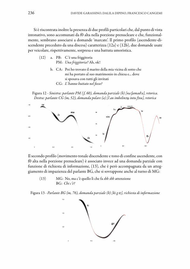
236 DAVIDE GARASSINO, DALILA DIPINO, FRANCESCO CANGEMI
Si è riscontrata inoltre la presenza di due profili particolari che, dal punto di vista intonativo, sono accomunati da f0 alta nella porzione prenucleare e che, funzional-mente, sembrano associarsi a domande ‘marcate’. Il primo profilo (ascendente-di-scendente preceduto da una discesa) caratterizza (12a) e (12b), due domande usate per veicolare, rispettivamente, sorpresa e una battuta umoristica.
(12) a. PB: C’è una friggitoria PM: Una friggitoria? Ah, ok!
b. CA: Poi ho trovato il marito della mia vicina di sotto che mi ha portato al suo matrimonio in chiesa e... dove si sposava con tutti gli invitati
CG: L’hanno buttato nel fosso?
Figura 12 - Sinistra: parlante PM ( f, 60), domanda parziale (b) [na ʃamadˑa], retorica. Destra: parlante CG (m, 52), domanda polare (a) [l an imbelinɔu intu fɔsu], retorica
Il secondo profilo (movimento tonale discendente e tono di confine ascendente, con f0 alta nella porzione prenucleare) è associato invece ad una domanda parziale con funzione di richiesta di informazione, (13), che è però accompagnata da un atteg-giamento di impazienza del parlante BG, che si sovrappone anche al turno di MG:
(13) MG: No, ma c’è quello lì che fa shh shh attenzione BG: Chi c’è?
Figura 13 - Parlante BG (m, 76), domanda parziale (b) [ki g ɛː], richiesta di informazione

PER UN APPROCCIO MULTIDIMENSIONALE ALLO STUDIO DELL’INTONAZIONE 237
In conclusione, è necessario ricordare che in questo lavoro abbiamo soltanto scalfito la multidimensionalità che dovrebbe essere il fondamento di un’analisi prosodica e pragmatica delle domande. Nei dati troviamo infatti altri indizi che potrebbero aiutarci a spiegare la variazione intonativa osservata. Ci limitiamo qui a commentare un ultimo caso:
(14) a. FM: Il diabete ancora non ce l’ho, dai. GM: Eh sì, il diabete. FM: E poi che cos’hai? GM: Poi ho una macchina.
b. FM: Ho un dodici qui, vedi? GM: Hai un dodici? FM: Sì, e tu che cos’hai?
Figura 14 - Sinistra: parlante FM (m, 74). Domanda parziale (i) [pɔi ˈkɔːsa ti g ɛː]. Destra: parlante FM (m, 74). Domanda parziale (n) [e ti ˈkɔːsa t ɛː]
Nonostante l’apparente somiglianza tra (14a) e (14b), i due esempi si differenzia-no per la struttura informativa. A differenza di (14a), in (14b) viene assegnato un valore contrastivo al pronome tonico soggetto ti (topic contrastivo, si vedano Büring 2003 e 2016), segnalato nel periogramma da un aumento di energia periodica e un movimento ascendente di f0.
6. ConclusioniUn primo (e preliminare) approccio multidimensionale all’analisi delle domande, coadiuvato dal periogramma, ci ha permesso non solo di confermare (in parte) i risultati della bibliografia precedente, ma anche di offrire un contributo originale allo studio delle domande nella varietà dialettale genovese.
Più specificamente, il nostro studio ha rivelato che le domande polari nel dia-letto di Genova rispecchiano la notevole variabilità già osservata nei dati relativi all’italiano regionale.
L’analisi delle domande parziali ha poi mostrato che queste ultime, a differen-za delle polari, non presentano mai nei nostri dati un movimento ascendente sulla

238 DAVIDE GARASSINO, DALILA DIPINO, FRANCESCO CANGEMI
tonica finale, ma si caratterizzano all’opposto, nella maggioranza dei casi, per una ripida discesa in corrispondenza della sillaba tonica.
Per quanto riguarda gli aspetti funzionali, si è osservata un’altra associazione con i profili melodici: le domande retoriche sembrano caratterizzate dal profilo di-scendente (-discendente), indipendentemente dalla loro struttura logico-semantica (al momento, però, i dati relativi alle domande polari e a quelle alternative sono troppo esigui per proporre generalizzazioni). Sempre in merito agli aspetti pragma-tici, alcune domande ‘marcate’ (così analizzate perché si accompagnano a certi stati d’animo ed emozioni o perché trasmettono contenuti umoristici) indicano anche un possibile ruolo dell’andamento melodico nella porzione prenucleare.
Da un punto di vista metodologico, questo lavoro ha mostrato anche i limiti di un tipo specifico di parlato (semi)spontaneo, rappresentato dal Map Task (anche nella nostra variante MMT), nell’analisi delle funzioni pragmatico-discorsive. Il tipo di interazione richiesta e l’enfasi sulle mosse fatiche nello svolgimento del com-pito sembrano limitare infatti lo spettro funzionale delle domande (soprattutto di quelle polari, ‘ridotte’ a mosse check e align). Infine, l’esiguità dei dati ha permesso di rinvenire soltanto delle tracce di altre dimensioni di variazione: è il caso, per esem-pio, del ruolo giocato dalla struttura informativa, ma anche delle caratteristiche so-ciolinguistiche dei nostri parlanti. L’attuale composizione del corpus, con i suoi forti squilibri in merito all’età e al sesso, non permette infatti un’analisi adeguata dell’e-ventuale impatto di queste variabili sulla realizzazione intonativa delle domande. Su questi ultimi punti ci riserviamo di ritornare in indagini future, sulla base di dati più numerosi e rappresentativi di altre manifestazioni di parlato spontaneo.
RingraziamentiIl presente studio è stato realizzato nell’ambito del progetto At the intersection between acoustic phonetics and information structure. An empirical investigation on the phonetic realization of vowel length in three Ligurian dialects (Nr. 100015_178932) del Fondo Nazionale Svizzero per la ricerca scientifica, che il primo e il secondo autore ringrazia-no per il sostegno. I tre autori desiderano inoltre ringraziare i revisori anonimi per i loro preziosi suggerimenti.
Riferimenti bibliografici
Albano Leoni, F. (2006). Il corpus CLIPS. Presentazione del progetto. http://www.clips.unina.it. Ultimo accesso: 13.03.2021.Albert, A., Cangemi, F., Ellison, M. & Grice, M. (2021). ProPer: PROsodic analysis with PERiodic energy. A workflow for periodic energy extraction and usage (with Praat and R). osf.io/jw2pvAlbert, A., Cangemi, F. & Grice, M. (2018). Using periodic energy to enrich acoustic representations of pitch in speech: A demonstration. In Proceedings of the 9th International Conference on Speech Prosody, Poznań, Poland, 13-16 June 2018, 804-808.

PER UN APPROCCIO MULTIDIMENSIONALE ALLO STUDIO DELL’INTONAZIONE 239
Amper-ita. Ultimo accesso: 13.03.2021. http://www.lfsag.unito.it/ricerca/amper-ita/#/map/italia/galloitalica/genova.Anderson, A.H., Bader, M., Gurman Bard, E., Boyle, E., Doherty, G., Garrod, S., Isard, S., Kowtko, J., McAllister, J., Miller, J., Sotillo, C., Thompson, H. & Weinert, R. (1991). The HCRC Map Task Corpus. In Language and Speech, 34(4), 351-366. https://doi.org/10.1177/002383099103400404.Arvaniti, A. (2022). The Autosegmental-Metrical model of intonational phonology. In Shattuck-Hufnagel, S., Barnes, J. (a cura di). Prosodic Theory and Practice. Cambridge, MA: The MIT Press, 25-83.Baker, R., Hazan, V. (2011). DiapixUK: task materials for the elicitation of multiple spontaneous speech dialogs. In Behavior Research Methods, 43(3), 761-770. https://doi.org/10.3758/s13428-011-0075-y.Beckman, M.E. (1997). A Typology of Spontaneous Speech. In Sagisaka Y., Campbell N. & Higuchi N. (a cura di). Computing Prosody. New York: Springer, 7-26.Boersma, P., Weenink, D. (2021). PRAAT: doing phonetics by computer. [Computer program] Version 6.1.40. http://www.praat.org/. Ultimo accesso: 13.03.2021.Büring, D. (2003). On D-trees, beans, and B-accents. In Linguistics and Philosophy, 26, 511-545. https://doi.org/10.1023/A:1025887707652.Büring, D. (2016). (Contrastive) Topic. In Féry, C., Ishihara, S. (a cura di), The Oxford Handbook of Information Structure. Oxford: Oxford University Press, 64-85.Canepari, L. (1980). Italiano standard e pronunce regionali. Padova: Cleup.Canepari, L. (1999). Il MaPI. Manuale di Pronuncia Italiana. Bologna: Zanichelli.Cangemi, F., Albert, A. & Grice, M. (2019). Modelling intonation: Beyond segments and tonal targets. In Calhoun, S., Escudero, P., Tabain, M. & Warren, P. (a cura di). Proceedings of the 19th International Congress of Phonetic Sciences, Melbourne, Australia, 5-9 August 2019, 572-576. Ultimo accesso: 21.05.2021. https://assta.org/proceedings/ICPhS2019/papers/ICPhS_621.pdf.Cangemi, F., Grice, M. (2016). The Importance of a Distributional Approach to Categoriality in Autosegmental-Metrical Accounts of Intonation. In Laboratory Phonology: Journal of the Association for Laboratory Phonology, 7(1): 9, 1-20. http://dx.doi.org/10.5334/labphon.28.Carletta, J., Isard, A., Isard, S., Kowtko, J.C., Doherty-Sneddon, G. & Anderson, A.H. (1997). The reliability of a dialogue structure coding scheme. In Association for Computational Linguistics, 23(1), 13-31.Castagneto, M. (2012). Il sistema di annotazione Pra.Ti.D tra gli altri sistemi di anno-tazione pragmatica. Le ragioni di un nuovo schema. In AIΩN. Annali del Dipartimento di Studi Letterari, Linguistici e Comparati. Sezione Linguistica 1, 103-146.Crocco, C. (2011). Profili melodici della varietà genovese. In Gili Fivela, B., Stella, A., Garrapa, L. & Grimaldi, M. (a cura di). Atti del VII Convegno Nazionale AISV. Contesto Comunicativo e variabilità nella produzione e percezione della lingua. Roma: Bulzoni, 188-199.Contini, M., Lai, J.P., Romano, A., Roullet, S., Moutinho, L., Coimbra, R.L. Pereira Bendiha, U. & Secca Ruivo, S. (2002). Un projet d’atlas multimédia proso-

240 DAVIDE GARASSINO, DALILA DIPINO, FRANCESCO CANGEMI
dique de l’espace roman. In Bel, B., Marlien, I. (a cura di). Proceedings of Speech Prosody 2002, Aix-en-Provence, Francia, 11-13 aprile 2002, 227-230.Couper-Kuhlen, E. (2012). Some truths and untruths about final intonation in con-versational questions. In De Ruiter, J.P. (a cura di). Questions: Formal, Functional and Interactional Perspectives. Cambridge: Cambridge University Press, 123-145.De Iacovo, V. (2017). Intonation analysis on some samples of Italian dialects: an instru-mental approach. Tesi di dottorato, Università degli Studi di Genova e Torino.Dipino, D., Filipponio, L. & Garassino, D. (2022). Manifestazioni della quantità voca-lica nella Liguria centro-occidentale: tipologia e metodologia. In Baranzini, L., Casoni, M. & Christopher, S. (a cura di). Linguisti in contatto 3. Ricerche di linguistica italiana in Svizzera e sulla Svizzera. Bellinzona: Osservatorio linguistico della Svizzera italiana, 17-37.Enfield, N.J., Stivers, T. & Levinson, S.C. (2010). Question-response sequences in conversation across ten languages: An introduction. In Journal of Pragmatics, 42, 2615-2619. https://doi.org/10.1016/j.pragma.2010.04.001.Feldhausen, I., Fliessbach, J. & Vanrell, M.d.M. (2018). Methods in prosody: A Romance language perspective. Berlin: Language Science Press.Filipponio, L., Garassino, D. & Dipino, D. (2019). Between phonology and typo-logy. Consonant duration in two Gallo-Italic dialects. In Piccardi, D., Ardolino, F. & Calamai, S. (a cura di). Gli archivi sonori al crocevia tra scienze fonetiche, informatica uma-nistica e patrimonio digitale. Milano: Officinaventuno, 269-291.Forner, W. (1975). Generative Phonologie des Dialekts von Genua. Hamburg: Buske.Forner, W. (1988). Areallinguistik I: Ligurien. In Holtus, G., Metzeltin, M. & Schmitt, C. (a cura di). Lexikon der romanistischen Linguistik (LRL), Tübingen: Niemeyer, 4, 453-469.Forner, W. (1989). La dialettologia ligure: risultati e prospettive. In Holtus, G., Metzeltin, M. & Pfister, M. (a cura di). La dialettologia italiana oggi. Studi offerti a Manlio Cortelazzo. Tübingen: Gunter Narr, 153-178.Forner, W. (2019). La situazione del ligure. In Toso, F. (a cura di). Il patrimonio linguisti-co storico della Liguria. Attualità e futuro. Savona: InSedicesimo, 47-68.Garassino, D., Cangemi, F. (2020). “No duration without intonation”. The interplay of lexical and post-lexical durational differences. In Proceedings of the 10th International Conference on Speech Prosody, Tokyo, Japan, 25-28 May 2020, 86-90.Garassino, D., Dipino, D. (2019). Vowel length in Intemelian Ligurian. An experimental and cross-dialectal investigation. In Calhoun, S., Escudero, P., Tabain, M. & Warren, P. (a cura di). Proceedings of the 19th International Congress of Phonetic Sciences, Melbourne, Australia, 5-9 August 2019, 122-126. https://assta.org/proceedings/ICPhS2019/. Ultimo accesso: 21.05.2021.Garassino, D., Loporcaro, M. & Schmid, S. (2017). La quantità vocalica in due dialetti della Liguria. In Bertini, C., Celata, C., Lenoci, G., Meluzzi, C. & Ricci, I. (a cura di). Fattori biologici e sociali nella variazione fonetica. Milano: Officinaventuno, 127-144.Garassino, D., Filipponio, L. (2021). The impact of information and prosodic structure on the phonetic implementation of vowel length in Ligurian. In Teixeira Kalkhoff, A., Selig, M. & Mooshammer, C. (a cura di). Prosody and conceptional variation. Situational

PER UN APPROCCIO MULTIDIMENSIONALE ALLO STUDIO DELL’INTONAZIONE 241
conditions of communication, degree of communicational planning, and activity types as para-meters for prosodic design. Bern: Peter Lang, 213-236.Gili Fivela, B., Avesani, C., Barone, M., Bocci, G., Crocco, C., D’Imperio, M., Giordano, R., Marotta, G., Savino, M. & Sorianello, P. (2015). Intonational pho-nology of the regional varieties of Italian. In Frota, S., Prieto, P. (a cura di). Intonation in Romance. Oxford: Oxford University Press, 140-197.Gili Fivela, B., Nicora, F. (2018). Intonation in Liguria and Tuscany. Checking for simi-larities across a traditional isogloss boundary. In Vietti, A., Spreafico, L., Mereu, D. & Galatà, V. (a cura di). Il parlato nel contesto naturale. Milano: Officinaventuno, 131-156.Grice, M., Savino, M. (2003a). Map Tasks in Italian: Asking questions about given, ac-cessible and new information. In Catalan Journal of Linguistics, 2, 153-180. https://doi.org/10.5565/rev/catjl.48.Grice, M., Savino, M. (2003b). Question type and information structure in Italian. In Proceedings of the international workshop Prosodic Interfaces, Nantes, France, 27-29 March 2003, 117-122.Grice, M., Savino, M. (2004). Information structure and questions: Evidence from task-oriented dialogues in a variety of Italian. In Gilles, P., Peters, J. (a cura di). Regional variation in intonation. Tubingen: Niemeyer, 161-187.Loporcaro, M. (2015). Vowel Length from Latin to Romance. Oxford: Oxford University Press.Mereu, D., Vietti, A. (2021). Dialogic ItAlian: the creation of a corpus of Italian spon-taneous speech. In Speech Communication, 130, 1-14. https://doi.org/10.1016/j.spe-com.2021.03.002.Ozerov, P. (2019). This is not an interrogative: the prosody of “wh-questions” in Hebrew and the sources of their questioning and rhetorical interpretations. In Language Sciences, 72, 13-35. https://doi.org/10.1016/j.langsci.2018.12.004.Pardo, J.S., Urmanche, A., Gash, H., Wiener, J., Mason, N., Wilman, S., Francis K. & Decker, A. (2019). The Montclair map task: Balance, efficacy, and efficiency in conversational interaction. In Language and Speech, 62(2), 378-398. https://doi.org/10.1177/0023830918775435.Rossi, M. (1998), Intonation in Italian. In Hirst, D., Di Cristo, A. (a cura di). Intonation Systems. A Survey of Twenty Languages. Cambridge: Cambridge University Press, 219-238.Roettger, T., Grice, M. (2019). The tune drives the text – Competing information channels of speech shape phonological systems. In Language Dynamics and Change, 9(2), 265-298. https://doi.org/10.1163/22105832-00902006.Savino, M. (2009). Intonational features for identifying regional accents of Italian. In Proceedings of the 10th Annual Conference of the International Speech Communication Association (Interspeech 2009), Brighton, UK, 6-10 September 2009, 2423-2426.Savino, M. (2012). The intonation of polar questions in Italian: Where is the rise? In Journal of the International Phonetic Association, 42(1), 23-48. https://doi.org/10.1017/S002510031100048X.Stivers, T., Enfield, N. (2010). A coding scheme for question–response sequences in conversation. In Journal of Pragmatics, 42(10), 2620-2626. https://doi.org/10.1016/j.prag-ma.2010.04.002.
242 DAVIDE GARASSINO, DALILA DIPINO, FRANCESCO CANGEMI
Torreira, F., Adda-Decker, M. & Ernestus, M. (2010). The Njimegen Corpus of Casual French. In Speech Communication, 52(3), 201-212. https://doi.org/10.1016/j.spe-com.2009.10.004.Toso, F. (1997). Grammatica del genovese. Varietà urbana e di koinè. Genova: Le Mani.Toso, F. (2010). Dialetti liguri. In Enciclopedia dell’Italiano, Treccani online. Ultimo ac-cesso: 13.06.2021 https://www.treccani.it/enciclopedia/dialetti-liguri_%28Enciclopedia-dell%27Italiano%29/.Van Engen, K.J., Baese-Berk, M., Baker, R.E., Choi, A., Kim, M. & Bradlow, A.R. (2010). The Wildcat Corpus of native-and foreign-accented English: Communicative effi-ciency across conversational dyads with varying language alignment profiles. In Language and speech, 53(4), 510-540. https://doi.org/10.1177/0023830910372495.Wagner, P., Trouvain, J. & Zimmerer, F. (2015). In defense of stylistic diversity in speech research. In Journal of Phonetics, 48, 1-12. https://doi.org/10.1016/j.wocn.2014.11.001.Xu, Y. (2011). Speech prosody: A methodological review. In Journal of Speech Sciences, 1(1), 85-115. https://doi.org/10.20396/joss.v1i1.15014.
DOI: 10.17469/O2108AISV000013
LOREDANA SCHETTINO, SIMON BETZ, FRANCESCO CUTUGNO, PETRA WAGNER
Hesitations and individual variability in Italian tourist guides’ speech1
This study concerns hesitation strategies that tourist guides may use to manage their speech, with particular attention to individual variability. Previous work has pointed out that hesitation phenomena may occur as a tool to structure discourse and gain visitors’ attention, and that linguistic idiosyncratic behavior may affect their production. Given these findings, the proposed investigation delves deeper into the linguistic analysis of formal, phonetic, and functional aspects of hesitations occurring in a small corpus of Italian tourist guides’ speech. It aims at describing the speaker-specific and common uses of hesitation phenomena and whether different types of hesitations and their phonetic features correlate with different discourse functions. From the results, it emerges a formal differentiation between hesitations involved in speech planning for lexical coding and for the structuring of information.
Keywords: speech, disfluencies, hesitations, pauses, individual variability.
1. IntroductionHuman spontaneous speech is characterized by the occurrence of phenomena connected to the online production process. Speakers can produce phonetic cues, like silent pauses or vocalizations, to suspend the speech delivery and gain extra-time for speech planning, or desert utterances due to change of projects, or alter uttered sequences that are considered somehow inaccurate or unfitting for the communicative intention. These phenomena affect to a certain extent speech fluency. For this reason, they are commonly referred to as ‘disfluencies’.
The definition of what is fluent and disfluent speech is rather problematic as the issue has been tackled from different angles, different research fields, with specific perspectives, approaches, and aims: investigations on speech disorders compare pathological and non-pathological speech; investigations on foreign or second-language learning compare native and non-native speech; psycholinguistics consider disfluencies as a window into the processes involved in speech production; linguists and phoneticians are interested in describing and framing disfluencies in relation to the linguistic systems; computational linguists are engaged in the definition of disfluency models for technological applications (see Lickley, 2015, for an overview).
1 Authors’ responsibilities – Loredana Schettino: conceptualization, data curation, writing – original draft (§1 – §7); Simon Betz: theoretical and methodological advice, writing – review & editing; Francesco Cutugno: supervision, writing – review & editing; Petra Wagner: supervision, writing – review & editing.

244 LOREDANA SCHETTINO, SIMON BETZ, FRANCESCO CUTUGNO, PETRA WAGNER
Despite field-specific interests and differences, numerous empirical studies have shown that speech disfluencies are not just occasional and idiosyncratic production errors, but regularly occur in speech (Shriberg, 1994; Bortfeld, Leon, Bloom, Schober & Brennan, 2001) and are naturally involved in the economy of speech as a flexible and efficient tool at speakers’ hand to manage the online processes of speech planning, coding, and articulation (Levelt, 1989; Allwood, Nivre & Ahlsén, 1990; Crocco, Savy, 2003; Voghera, 2017). In fact, speakers can correct already uttered sequences using Repairs or Backward-Looking Disfluencies, that is the deletion, insertion, or substitution of speech material. Furthermore, speakers can gain some extra time to organize the output message inserting pauses, fillers, lengthenings, that are commonly subsumed under the category of Hesitations or Forward-Looking Disfluencies (Ginzburg, Fernández & Schlangen, 2014).
The occurrences and realizations of disfluencies were found to vary and were associated with different functions in discourse due to contextual and individual factors. (Bortfeld et al., 2001; Betz, Lopez Gambino, 2016, a.o.). Further, it has been highly debated whether and when disfluencies may be intentionally produced to signal something or exert a certain effect. As a matter of fact, up to our knowledge, there is still no evidence of speakers’ deliberate control over their production (Corley, Stewart, 2008).
This study aims at investigating hesitation strategies that tourist guides may more or less consciously use to manage their speech, with particular attention to individual variability.
The article is structured as follows: §2 presents the literature concerning hesitation phenomena and the factors affecting their productions; §3 presents the general and specific aims of the study; §4 describes the linguistic data, the annotation process, and the parameters of the linguistic analysis; in §5 and §6 the results of the analysis are reported and discussed.
2. Related WorkThe term “hesitations” is commonly used in literature to cover a set of speech phenomena, like silent pauses, fillers, lengthenings, that realize a temporary suspension in the utterance delivery (Lickley, 2015). In the last 40 years, after the seminal work by Chafe (1980), research on hesitations has embraced a “positive” view that acknowledges the role played by these elements in speech, that is to reduce the temporal pressure due to the simultaneity of planning, production, and reception processes. On the one hand, they gain valuable time for speakers to manage the online process of speech production. On the other hand, they provide extra time for the listeners to process information (Chafe, 1980; Levelt, 1989; Corley, Hartsuiker, 2003).
Empiric investigations, including corpus-based and experimental studies, have analyzed the meaning and the factors that affect the production of hesitations (see Rochester, 1973; Crocco et al., 2003; Eklund, 2004 for a review). To this end, the

HESITATIONS AND INDIVIDUAL VARIABILITY 245
consideration of the context of occurrence is crucial given that these phenomena lack conceptual meaning2 (Crible, 2018).
Generally, the occurrence of hesitation phenomena was observed to be mainly connected to moments that require a higher cognitive load in the speech planning process: a) the conceptualization and formulation of a new utterance (macro-planning, Levelt, 1989; Oviatt, 1995; Bortfeld et al., 2001); b) the search for a specific lexical item (micro-planning, Schnadt, Corley, 2006; Hartsuiker, Notebaert, 2009), for a word with low contextual probability (Beattie, Butterworth, 1979) or a word that is more difficult to retrieve for the speaker, hence low in “codability” (Chafe, 1980); c) the selection of new information in discourse (Arnold, Fagnano & Tanenhaus, 2003). In fact, it was also highlighted that hesitation phenomena play a role in structuring discourse and may indicate to the listener the arrival of important information (Chafe, 1980; Allwood et al., 1990; Kosmala, Morgenstern, 2017). Furthermore, the communicative situation, e.g., the linguistic register and the argument under discussion were found to affect the incidence of hesitations (Bortfeld et al., 2001; Moniz, Batista, Mata & Trancoso, 2014; Crible, Bunt, 2016).
Hence, if lacking in conceptual content, hesitations carry procedural meaning conveying valuable information on speech planning, structuring, and speakers’ disposition (Cataldo, Schettino, Savy, Poggi, Origlia, Ansani, Sessa & Chiera, 2019; Betz, 2020). Further studies have shown that the phonetic-prosodic features of these elements correlate with the contextual function and can discriminate between more or less “felicitous” occurrences in discourse (Swerts, 1998; Moniz, Trancoso & Mata, 2010).
More specifically, silent pauses are, with filled pauses, one of the most studied types of hesitation phenomena. After the highly influential analysis by Sacks and colleagues (Sacks, Schegloff & Jefferson, 1978), numerous studies have acknowledged and investigated the communicative role of silence in conversation. It was found to range from emphasizing key elements (Duez, 1997; Strangert, 2003), marking discourse boundaries (Boomer, Dittman, 1962; Esposito, Stejskal, Smékal & Bourbakis, 2007), working as discourse marker for turn-taking management (Ephratt, 2008), to manifesting hesitation in speech or troubles in information processing and need for clarification. In particular, longer silences have been associated with speech processing problems (Chowdhury, Stepanov, Danieli & Riccardi, 2017; Schettino, Di Maro & Cutugno, 2020). In some studies, silences were identified as hesitant when longer than an established temporal threshold (200 ms in Beattie et al., 1979; according to the syntactic position, 200 or 500 ms in O’Shaugnessy, 1992; 60 ms in Kendall, 2009, a.o.). However, this approach is rather problematic as in some contexts silences that are shorter than these thresholds may be perceived as hesitant (Eklund, 2004; Lickley, 2015).
Numerous investigations also involved filled pauses and the correlation between their phonetic-prosodic features (segmental content, pitch values, position, length)
2 As proposed in Relevance Theory (Blakemore 2002; Wilson 2011; Wilson, Sperber, 2012), different types of encoded meaning may be identified, i.e., “conceptual meaning”, which refers to entities or concepts, and “procedural meaning”, which gives the coordinates for the interpretation process.

246 LOREDANA SCHETTINO, SIMON BETZ, FRANCESCO CUTUGNO, PETRA WAGNER
and the associated function in context. More specifically, a longer duration is reported for filled pauses that occur at the beginning of a phrase (Swerts, 1998), that introduce a new part of the utterance (Horváth, 2010), or manifest problems in the retrieval of a specific word (Cataldo et al., 2019). The controversial claim that filled pauses may be considered as proper words intentionally used by speakers to signal upcoming delays in speech delivery was strongly debated (Clark, Fox Tree, 2002). As a matter of fact, it was highlighted that there is still no evidence of speakers’ deliberate control over their production (O’Connell, Kowal, 2005; Corley et al., 2008; Finlayson, Corley, 2012). So, it was argued that filled pauses, much like intonation, may well be unconsciously used by speakers in aiming for a certain effect (Kjellmer, 2003) and “acquire their communicative function as pragmatic markers when interpreted by the listener” (Tottie, 2016: 100). Generally, speech planning can be considered the basic function of filled pauses, furthermore, their use was found to be connected to the search for a specific word, discourse structuring, turn-taking management, drawing the listener’s attention on an upcoming semantically heavy element, or marking that a delicate or “dispreferred” action is about to follow (Kjellmer, 2003; Schegloff, 2010; Kosmala, Morgenstern, 2018; Tottie, 2020).
As for lexical fillers, they are commonly subsumed under the multi-functional class of discourse markers and not always acknowledged among hesitation phenomena (Schiffrin, 1987; Bazzanella, 2006; Crible, 2018). However, as in filled pauses, the primary function of discourse markers used as fillers is gaining extra time for speech planning. Then, due to their multifunctional nature, they may also provide valuable meta-discursive information about turn-taking management, discourse structure, and the speaker’s disposition (Bazzanella, 2006; Schettino, Cataldo, 2019).
Finally, among the voiced hesitant pauses, the lengthenings of segmental material can be identified. Pitch values were found to distinguish hesitant prolongations from non-disfluent ones, i.e., due to accentuation. In particular, the first ones are generally realized with lower pitch range and flat contour, whereas the second ones with higher pitch range and rising contour (Eklund, 2001; Moniz, 2013; Betz, 2020). However, the study of the way lengthenings work in discourse and speech planning has only in the past about ten years gained more attention (Moniz, Mata & Céu Viana, 2007; Betz, Zarrieß, Székely & Wagner, 2019).
In different languages filled pauses were found to be on average longer than lengthenings (Swedish: Eklund, 2001, 2004; German: Betz, Eklund & Wagner, 2017; Italian: Di Napoli, 2020; Cataldo et al., 2019).
Besides these general observations, studies on a range of languages and speaking styles report significant individual variability in the production of disfluencies (Shriberg, 2001; Eklund 2004; Roberts, Meltzer & Wilding, 2009; Moniz et al., 2014; Kosmala et al., 2018; Cataldo et al., 2019). Specific investigations confirm this finding by describing the emergence of speaker-dependent pausing strategies, i.e., in the choice of using silences, lengthenings, or filled pauses for the need of speech planning (Van Donzel, Koopmans-van Beinum, 1996). In particular, Betz and Lopez Gambino (2016) analyzed the individual variability in a dataset of German spontaneous speech

HESITATIONS AND INDIVIDUAL VARIABILITY 247
produced by six speakers and elicited via a Wizard of Oz experiment to control for time management. They report three main tendencies: a general avoidance of fillers and a high tolerance for silence; a balanced use of both silent and filled pauses; avoidance of both and reliance on low-content words for hesitation purposes. Furthermore, it was observed that the individual hesitation strategies characterize speakers’ production also when speaking a second language (Fehringer, Fry, 2007). So, based on the assumption that speech planning and production strategies may respond to individual psycho- and socio-linguistic demands, McDougall and Duckworth (2017) highlighted the speaker-discriminating role of disfluency production, which provides a further tool for forensic phoneticians.
3. Research AimThis study is part of a project that aims at modeling the occurrence of hesitation phenomena in Italian semi-spontaneous discourse for technological applications. It has been developed from the CHROME project – Cultural Heritage Resources Orienting Multimodal Experience – generally aimed at modeling multimodal data for the design of Virtual Agents serving in museums (Origlia, Savy, Poggi, Cutugno, Alfano, D’Errico, Vincze & Cataldo, 2018).
The observations reported in the previous section §2 support the assumption that hesitation phenomena contribute to the efficacy of the interaction. So, modeling their occurrence in discourse may be useful for both improving our understanding of conversational dynamics and the implementation of dynamic and efficient human-machine interactions. More specifically, Incremental Spoken Dialogue Systems would benefit from the ability to insert hesitation phenomena as it would provide a set of tools to cover the time needed for response processing, to signal the ongoing process, and it would result in more natural productions (Adell, Escudero & Bonafonte, 2012; Skantze, Hjalmarsson, 2013; Betz, Carlmeyer, Wagner & Wrede, 2018; Origlia, Savy, Cataldo, Schettino, Ansani, Sessa, Chiera & Poggi, 2019).
Hence, the proposed study delves deeper into the linguistic analysis of structural, phonetic, and functional aspects of hesitations in a corpus of tourist guides’ speech and addresses the following research questions:1. What individual strategies can speakers use when hesitating?2. How do different types of hesitations and their duration correlate with different
discourse functions?
4. Methodology4.1 Corpus and dataset
To address the research questions, we conducted a corpus-based analysis on a dataset extracted from the CHROME corpus (Origlia et al., 2018). The corpus consists of audio-visual recordings of three tourist guides (G) each leading four visits (V) at

248 LOREDANA SCHETTINO, SIMON BETZ, FRANCESCO CUTUGNO, PETRA WAGNER
San Martino’s Charterhouse in Naples. Each visit is organized into six points of interest (P). The selected data concern the presentation of the same point of interest (P01, i.e., the Pronao, the entrance of the Church) in two different visits per guide, which amounts to approximately 80 minutes of semi-spontaneous speech (Table 1 reports duration, number of uttered words, and speech rate per speaker).
Given the setting and the communicative goal of tourist guides, the elicited speech presents specific characteristics: a high degree of discourse planning, as the production is based on a partially pre-structured descriptive text; a low degree of interaction and participation in the discourse construction, because of the asymmetrical relationship between the guide and the audience. Hence, this kind of speech can be defined as semi-spontaneous and semi-monological (Voghera, 2017; Cataldo et al., 2019).
Table 1 - Selected Dataset
Speaker File – ID Duration (min) Words words/
minute
G01 V01P01 11:33 1491 129.0G01 V02P01 13:22 1705 129.2G02 V01P01 16:00 2788 174.3G02 V02P01 13:32 2349 173.6G03 V01P01 14:29 2138 147.6G03 V03P01 11:48 1706 145.1Total 80:34 12183 151.1
4.2 Linguistic Analysis
The scheme adopted for the annotation of disfluency phenomena is a revised version of the one tested in a previous pilot study (Cataldo et al., 2019). The system integrates the identification of disfluencies’ formal structures and their functions in the context of occurrence (Schettino, Cataldo, Alfano & Leo, forthcoming) and includes the following levels of annotation:1. Disfluency Model, on the first level, the macro-structure of disfluencies is labeled.
Namely, the region to be repaired, the repaired one, and the one in which the delay occurs (see Shriberg, 1994).
2. Disfluency Structure, the second level serves for labeling the micro-structure embodying the disfluency. Here, disfluent items are categorized as Insertion, Deletion, Substitution, Repetition, Silent Pause, Lengthening, Filled Pause, Lexicalized Filled Pause (Eklund, 2004).
3. Disfluency Function, on the third level, each item is assigned its macro-function, Backward-Looking or Forward-Looking (Ginzburg et al., 2014).
4. Hesitation Function, on a fourth level, Forward-Looking items – hesitations marking a temporary delay in speech – are associated with more specific functions regarding their co-text.

HESITATIONS AND INDIVIDUAL VARIABILITY 249
Unlike the categories of the first three levels, on the fourth functional level, given the fact that hesitation phenomena may carry out more than one function, categories are not mutually exclusive.
The procedure was conducted using the work tool ELAN (2020, Sloetjes, Wittenburg, 2008), a software for multilevel linguistic annotations, which allows to assign labels from pre-specified vocabularies and define the relationship between categories per each tier.
In this study the following hesitation types are considered:– Silent Pause (SP) identifies marked silences perceived as a hesitant pause in the
context of occurrence (breath pauses are not included);– Filled Pause (FP) identifies non-verbal filler, vocalizations and/or nasalizations,
i.e., eeh, ehm, mhh;– Lexicalized Filled Pause (LFP) identifies verbal fillers, meaning lexical items that
are semantically strongly bleached in their context of occurrence, i.e., well, let’s say, so, a.o.;
– Lengthening (LEN) identifies marked prolongation of segmental material (Betz, 2020).
The identification of these phenomena does not depend on absolute measures but is related to the context of occurrence, which entails subjective perceptual judgment. Hence, its reliability was tested measuring Cohen’s K for the ratings by two expert annotators (K = 0.91, high agreement; Landis, Koch, 1977).
Each type of hesitation is then associated with specific functions according to their context of occurrence. Functions were classified as follows:– Word Searching (WS) is the label assigned to items involved in the lexical
retrieval and selection of a target word (Tottie, 2020), for example to the filled pause, silent pause, lengthening, and repetitions preceding the word “beauty” in the following utterance:
(a) potete intuire <ehm> <sp> la<aa> la bellezza” “you can grasp <uhm> <sp> the<ee> the beauty”
– Structuring (STR) is the label assigned to items that play a structuring role in discourse occurring on syntax (clause) and information structure (topic-comment) boundaries. The following utterance provides an example of a silent pause and a filled pause co-occurring on the boundary between two clauses, in both cases a lengthening and a filled pause occur between the topic and the relative comment.
(b) “la<aa> Certosa di San Martino qui a Napoli<ii> <ehm> ha almeno due anime <sp> <eeh> una<aa> <ehm> racconta la storia...”
“the<ee> Charterhouse here in Neaples<vv> <ehm> has two souls <sp> <eeh> one<ee> <ehm> tells the story...”
– Focusing (FOC) is the label assigned to items preceding keywords or key concepts, i.e., semantically heavy and often emphasized elements in the context (Kjellmer,

250 LOREDANA SCHETTINO, SIMON BETZ, FRANCESCO CUTUGNO, PETRA WAGNER
2003). The following utterance provides an example of a silent pause preceding the main information in the utterance: the origin of the Charterhouse.
(c) “quindi la<aa> Certosa ha un’origine <sp> trecentesca” “so the<ee> Charterhouse has a <sp> 14th century origin”
– Hesitative (HES) is the category standing for hesitations’ basic function of speech planning. It is assigned to items for which no other function can be identified.
(d) “non possiamo vedere<ee> molto bene” “we can’t see<ee> it properly”
Also in this case the robustness of the categorization was tested measuring Cohen’s K for the inter-annotator agreement (K = 0.73, substantial agreement; Landis et al., 1977).
Furthermore, the analysis concerns the duration variation of SP, FP, and LEN as a function of hesitations type and function.
4.3 Statistical Analysis
The statistical analysis was performed using the R software (R Core Team, 2020). To define speakers’ systematic preferences and strategies, the occurrence of the selected hesitation types was modeled as a function of the associated function and the speaker. As reported in the previous paragraph, §4.2, four types of hesitation phenomena are considered, hence a Multinomial Logistic Regression Model was built using the ‘multinom’ function from the ‘nnet’ package (Venables, Ripley, 2002). The model included Hesitation Type as multinomial dependent variable, whereas Speaker and Function as interacting independent variables. This approach is useful to consider the speaker’s effect on the occurrence of hesitations and to observe their interaction with the effect of function, but to inspect the way hesitations are commonly used, a method that allows controlling for individual variability is needed.
Therefore, to analyze the role of functions on the occurrence of the four different types of phenomena independently from speaker-specific strategies, Mixed Models were implemented selecting Speaker and Item as random effects (‘lme4’ package, Bates, Maechler, Bolker & Walker, 2015). More specifically, to determine whether and how the use of hesitation types depends on the functions, Generalized Linear Mixed Models were fitted. In this case, each type of hesitation was processed as binomial dependent variable and Function was selected as the independent variable. Furthermore, Linear Mixed Models were fitted to inspect the systematic variation of hesitations duration, introduced as the dependent variable, as a function of Type and Function, selected as interacting independent variables.
Post-hoc analyses were conducted to inspect the levels within the main effects and the interactions using pairwise comparisons (‘emmeans’ package, Length, 2020). P-values were calculated using Tukey’s HSD adjustment.

HESITATIONS AND INDIVIDUAL VARIABILITY 251
5. Results5.1 Idiosyncratic Hesitation Strategies
In the selected dataset 1158 hesitation items occur. Among these, as illustrated in Figure 1, lexical fillers are by far the most frequent (45%), filled pauses and lengthenings are equally frequent (21%), whereas silent pauses are less frequent (13%).
Figure 1 - Frequency of hesitation types per speaker
Results confirm and dig deeper into some of the findings by Cataldo et al. (2019) reporting the emergence of idiosyncratic linguistic behaviors. As shown in Table 2, the occurrences are unevenly distributed across the three speakers (G01, G02, G03). Indeed, G01 produces approximately 20 hesitations per minute and 16 per 100 words, which is about twice as much as the productions by the other two guides. The statistical computation yielded significant results as for the speaker effect and the interaction between speaker and function, which confirms that speakers systematically adopt different strategies in the choice of hesitation phenomena and associated pragmatic functions (see Fig. 1 and Fig. 2).
Table 2 - Per minute, per word hesitation rate (column 2 and 3) and occurrences of hesitations by Speaker
Speaker n° hes/minute
n° hes/100 word LEN FP LFP SP
G01 20.12 16 144 (30%) 166 (34%) 98 (20%) 78 (16%)G02 11.55 7 64 (19%) 42 (13%) 210 (63%) 19 (6%)G03 12.10 8 32 (10%) 32 (10%) 198 (63%) 53 (17%)

252 LOREDANA SCHETTINO, SIMON BETZ, FRANCESCO CUTUGNO, PETRA WAGNER
Table 3 - Significant results yielded by the post-hoc analysis for the multinomial logistic models
HesType Function Speakerscontrast Estimate SE df t.ratio p.value
LEN / G01 – G03 0.113 0.035 36 3.255 0.007FP / G01 – G02 0.172 0.028 36 6.145 <.0001FP / G01 – G03 0.103 0.039 36 2.641 <.0001
LFP / G01 – G02 -0.330 0.029 36 -11.328 <.0001LFP / G01 – G03 -0.129 0.030 36 -4.302 <.0001SP / G01 – G02 0.113 0.018 36 6.156 <.0001SP / G02 – G03 -0.199 0.036 36 -5.416 <.0001
LEN FOC G01 – G02 0.100 0.034 36 2.909 0.0166LEN FOC G01 – G03 0.088 0.033 36 2.632 0.0325
FP STR G01 – G02 0.371 0.053 36 6.956 <.0001FP STR G01 – G03 0.318 0.058 36 4.649 0.0001
LFP HES G01 – G02 -0.334 0.066 36 -5.020 <.0001LFP HES G02 – G03 0.350 0.080 36 4.347 0.0003LFP WS G01 – G02 -0.120 0.053 36 -2.283 0.0711LFP WS G02 – G03 0.180 0.053 36 3.376 0.0049SP HES G01 – G03 -0.413 0.116 36 -3.543 0.0031SP HES G02 – G03 -0.457 0.115 36 -3.956 0.0010
The post-hoc analysis reveals that as compared to the other two speakers: G01 uses significantly more filled pauses (34%) and lengthenings (30%), fewer lexical fillers (20%); G02 uses fewer silent pauses (6%). Also, concerning the interaction between hesitation type and function, as compared to the other guides’ speech, in G01’s speech, more lengthenings are used with focusing function (FOC), and more filled pauses with structuring function (STR); in G02’s speech, more lexical fillers are used to convey hesitative (HES) and word searching (WS) function; in G03’s speech, more silent pauses are used for the hesitative function (significant results are reported in Table 3).
5.2 Hesitation Type and Functions
Besides the observed inter-speakers variability, the mixed models used to investigate the general systematic relationship between hesitation types and the function associated in context yielded significant results (Fig. 2).

HESITATIONS AND INDIVIDUAL VARIABILITY 253
Figure 2 - Frequency of hesitation functions per speaker grouped by hesitation type
Figure a - LEN ~ Function Figure b - FP ~ Function
Figure c - LFP ~ Function Figure d - SP ~ Function
Figure 2a shows that lengthenings are more frequently associated to hesitative and word searching functions and significantly less to structuring (Est: -2.17; SE: 0.28; z: -7.75; p < .001) and to focusing (Est: -2.33; SE: 0.40; z: -5.80; p < .001). Similarly, Figure 2b shows that fillers generally carry out word searching functions (Est: 0.62; SE: 0.19; z: 3.18; p < .001) and significantly less often focusing functions (Est: -4.10; SE: 0.95; z: -4.30; p < .001).
Conversely, as illustrated in Figure 2c, lexical fillers are more frequently associated to structuring (Est: 1.76; SE: 0.24; z: 7.10; p < .001) and focusing functions (Est: 2.78; SE: 0.27; z: 9.97; p < .001).
Lastly, a similar trend is reported for silent pauses in Figure 2d. In this case, silent pauses are systematically less associated to the hesitative function (Est: -2.34; SE: 0.49; z: -4.76; p < .001).
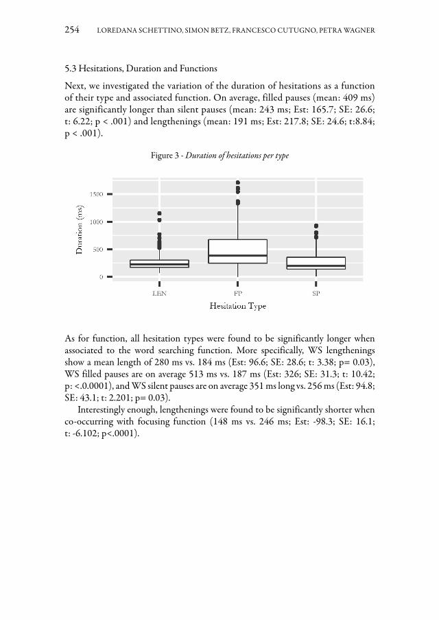
254 LOREDANA SCHETTINO, SIMON BETZ, FRANCESCO CUTUGNO, PETRA WAGNER
5.3 Hesitations, Duration and Functions
Next, we investigated the variation of the duration of hesitations as a function of their type and associated function. On average, filled pauses (mean: 409 ms) are significantly longer than silent pauses (mean: 243 ms; Est: 165.7; SE: 26.6; t: 6.22; p < .001) and lengthenings (mean: 191 ms; Est: 217.8; SE: 24.6; t:8.84; p < .001).
Figure 3 - Duration of hesitations per type
As for function, all hesitation types were found to be significantly longer when associated to the word searching function. More specifically, WS lengthenings show a mean length of 280 ms vs. 184 ms (Est: 96.6; SE: 28.6; t: 3.38; p= 0.03), WS filled pauses are on average 513 ms vs. 187 ms (Est: 326; SE: 31.3; t: 10.42; p: <.0.0001), and WS silent pauses are on average 351 ms long vs. 256 ms (Est: 94.8; SE: 43.1; t: 2.201; p= 0.03).
Interestingly enough, lengthenings were found to be significantly shorter when co-occurring with focusing function (148 ms vs. 246 ms; Est: -98.3; SE: 16.1; t: -6.102; p<.0001).

HESITATIONS AND INDIVIDUAL VARIABILITY 255
Figure 4 - Duration of hesitations per type and function
6. DiscussionThe interpretation of the presented results must consider the specific features of the analyzed speech. As previously mentioned, tourist guides’ speech is mostly characterized by a high degree of speech planning and a descriptive-informative style that results from the type of asymmetrical relationship between the interlocutors: the guide and the tourists. In this setting, the speaker aims to engage the listeners and provide the required information clearly and efficiently. So, the consistent occurrence of hesitation phenomena in these pre-scripted, repeated productions corroborates the assumption of hesitations’ supportive role in achieving the communicative purpose in the desired manner rather than obstructing it. For this reason, studying hesitation phenomena in this speech style, i.e., the informative style, proves to be particularly helpful to get insight of how they work as linguistic resources.
The analysis confirms that speakers choose different specific hesitation strategies (Cataldo et al., 2019), which, as observed by McDougall and Duckworth (2017), may reflect individual responses to psycho- and socio-linguistic demands. Indeed, the first guide manifests a higher tolerance for hesitations producing twice as many as the other two guides, particularly, several filled pauses and lengthenings. In her production, more than in the others’, filled pauses are also used to mark sentence and topic boundaries and lengthenings to mark semantically heavy keywords, besides buying time for the online speech processing, in what could be defined as a more spontaneous ‘on the fly’ production. The second guide produces fewer hesitations, more specifically, she avoids hesitant silent pauses altogether and tends to avoid lengthenings and filled pauses relying on lexicalized filled pauses for word searching and general hesitation functions as well as for structuring and focusing. Then, the third guide adopts a more controlled, ‘rhetorical’ style, using mainly lexicalized
256 LOREDANA SCHETTINO, SIMON BETZ, FRANCESCO CUTUGNO, PETRA WAGNER
filled pauses and silent pauses to structure her discourse and to mark important information, besides general hesitation. The very few lengthenings and filled pauses she produces are associated with casual word retrieval difficulties.
Overall, in the analyzed speech, hesitation is mostly marked by lexicalized filled pauses, which means that the three tourist guides prefer to cover the time needed for speech planning producing fillers that consist of a proper lexical form (though semantically bleached and not adding anything to the propositional content of the utterance; Bazzanella, 2006; Crible, 2018) rather than other hesitation pauses such as vocalizations and silences that may be perceived as being more salient and disruptive (Betz, Bryhadyr, Kosmala & Schettino, 2021).
Despite interspeaker variability, a structural and phonetic differentiation emerges between hesitations associated with different functions.
More specifically, lengthenings and filled pauses are mostly involved in word retrieval problems and general planning problems, rather than structuring discourse. Conversely, lexicalized filled pauses and silent pauses are mostly associated with the structuring and focusing functions.
Looking at the results concerning duration values, across hesitation types, phenomena associated with the word searching function suspend speech delivery for more time, which leads to acknowledging the search for and the selection of a specific lexical item as more time-consuming processes.
Furthermore, the opposition between the word searching and focusing functions was found to be encoded in lengthenings’ duration, respectively longer and shorter.
Given these results, the higher duration registered for filled pauses as compared to silent pauses and lengthenings (also in Eklund, 2001; 2004; Betz et al., 2017; Di Napoli, 2020; Cataldo et al., 2019) may be explained by the fact that filled pauses are the type of hesitation more frequently associated to the word searching function.
The observed structural and phonetic differentiation of hesitation phenomena could be interpreted as a reflection of different processes involved in speech planning. Two main processes could be identified, namely, on the one end the conceptualization and translation of thought into linguistic objects (lexical-semantic level), on the other the structurization of information (pragmatic level). Indeed, as already observed by Levelt (1983, 1989) and Chafe (1980) speakers may need time to check for what to say, how to code their thought into language, and make sure that their communicative intention is conveyed appropriately and efficiently.
The described analysis has contributed to shedding light on the way speakers may use hesitation phenomena as resources to efficiently manage their speech while aiming at reaching their communicative goal, in this case, providing the required information clearly and efficiently. Although to date it is not clear the degree of consciousness involved in this process, it emerged that speakers may enact different hesitation strategies by employing these phenomena in the way that they deem as most suitable and appropriate to the task. This choice may further be subjected to intra-speaker variation: synchronically – due to the specific communicative situation, the roles of the interlocutors, the speakers’ degree of self-consciousness

HESITATIONS AND INDIVIDUAL VARIABILITY 257
as they speak – and diachronically – due to the over time ongoing building of the individual cognitive representations that underlie language use (respectively referred to as “intra-speaker” and “intra-individual” variation in Bülow, Pfenninger, 2021).
7. ConclusionTo conclude, this study has contributed to describing the use of hesitations as speech management phenomena in Italian tourist guides’ speech considering the relevance of inter-speaker variability.
The identification and modeling of this kind of linguistic behavior provide influential findings for a range of technological speech applications such as interactive speech synthesis. In particular, the performances, i.e., the naturalness and communicative efficacy, of a system supporting a Virtual Agent serving in museums may result improved by a theoretically motivated insertion of hesitations. Furthermore, the observation of speaker-specific strategies leads us to be cautious towards developing synthesis systems based on averaged behaviors. Follow-up studies are meant to experimentally evaluate listeners’ perception to test relevant corpus-based observations.
Finally, this investigation has concerned a specific type of speech and the production of a limited number of speakers, which works for the intended specific application. However, future analyses should consider further speaking styles gathered from a larger number of speakers to gain a better understanding of hesitation pauses’ communicative functions and their contribution to discourse and communication.
AcknowledgementsWork funded by the Italian National Project PRIN Cultural Heritage Resources Orienting Multimodal Experiences (CHROME)(B52F15000450001).
Bibliography
Adell, J., Escudero, D. & Bonafonte, A. (2012). Production of filled pauses in concatenative speech synthesis based on the underlying fluent sentence. In Speech Communication, 54 (3), 459-476. https://doi.org/10.1016/j.specom.2011.10.010Allwood, J., Nivre, J. & Ahlsén, E. (1990). Speech management – on the non-written life of speech. In Nordic Journal of Linguistics, 13, 3-48. https://doi.org/10.1017/S0332586500002092Arnold, J.E., Fagnano, M. & Tanenhaus, M.K. (2003). Disfluencies signal theee, um, new information. In Journal of psycholinguistic research, 32 (1), 25-36. https://doi.org/10.1023/A:1021980931292

258 LOREDANA SCHETTINO, SIMON BETZ, FRANCESCO CUTUGNO, PETRA WAGNER
Bates, D., Maechler, M., Bolker, B. & Walker, S. (2015). Fitting Linear Mixed-Effects Models Using lme4. In Journal of Statistical Software, 67 (1), 1-48. https://doi.org/10.18637/jss.v067.i01Bazzanella, C. (2006). Discourse markers in Italian: towards a ‘compositional’ meaning. In Approaches to discourse particles, 1, 504-524.Beattie, G.W., Butterworth, B.L. (1979). Contextual probability and word frequency as determinants of pauses and errors in spontaneous speech. In Language and speech, 22 (3), 201-211. https://doi.org/10.1177/002383097902200301Betz, S. (2020). Hesitations in Spoken Dialogue Systems. PhD Dissertation, Universität Bielefeld.Betz, S., Lopez Gambino, M.S. (2016). Are we all disfluent in our own special way and should dialogue systems also be?. In Proceedings of Elektronische Sprachsignalverarbeitung (ESSV), Leipzig, Germany, 2-4 March 2016, 81.Betz, S., Eklund, R. & Wagner, P. (2017). Prolongation in German. In Proceedings of DiSS 2017 The 8th Workshop on Disfluency in Spontaneous Speech, Stockholm, Sweden, 18-19 August 2017, 13-16.Betz, S., Carlmeyer, B., Wagner, P. & Wrede, B. (2018). Interactive hesitation synthesis: modelling and evaluation. In Multimodal Technologies and Interaction, 2 (1), 9. https://doi.org/10.3390/mti2010009Betz, S., Zarriess, S., Székely, É. & Wagner, P. (2019). The greennn tree-lengthening position influences uncertainty perception. In 20th Annual Conference of the International Speech Communication Association: Crossroads of Speech and Language, INTERSPEECH 2019. Graz, Austria, 15-19 September, 3990-3994. https://doi.org/10.21437/Interspeech.2019-2572Betz, S., Bryhadyr, N., Kosmala. L. & Schettino, L. (2021). A Crosslinguistic Study on the Interplay of Fillers and Silences. In Proceedings of DiSS 2021, The 10th Workshop on Disfluency in Spontaneous Speech, Paris, France, 25-27 August 2021, 47-52.Blakemore, D. (2002). Relevance and linguistic meaning: The semantics and pragmatics of discourse markers (Vol. 99). Cambridge: Cambridge University Press. https://doi.org/10.1017/CBO9780511486456Boomer, D.S., Dittmann, A.T. (1962). Hesitation pauses and juncture pauses in speech. In Language and speech, 5 (4), 215-220. https://doi.org/10.1177/002383096200500404Bortfeld, H., Leon, S.D., Bloom, J.E., Schober, M.F. & Brennan, S.E. (2001). Disfluency rates in conversation: Effects of age, relationship, topic, role, and gender. In Language and speech, 44 (2), 123-147. https://doi.org/10.1177/00238309010440020101Bülow, L., Pfenninger, S.E. (2021). Introduction: Reconciling approaches to intra-individual variation in psycholinguistics and variationist sociolinguistics. In Linguistics Vanguard, 7 (s2), 1-10. https://doi.org/10.1515/lingvan-2020-0027Cataldo, V., Schettino, L., Savy, R., Poggi, I., Origlia, A., Ansani, A., Sessa, I. & Chiera, A. (2019). Phonetic and functional features of pauses, and concurrent gestures, in tourist guides’ speech. In XV Convegno Nazionale AISV. Gli archivi sonori al crocevia tra scienze fonetiche, informatica umanistica e patrimonio digitale. Studi AISV 6, 205-231.
HESITATIONS AND INDIVIDUAL VARIABILITY 259
Chafe, W. (1980). Some reasons for hesitating. In Dechert, H.W., Raupach, M. (Eds.), Temporal variables in speech: Studies in Honour of Frieda Goldman-Eisler. The Hague: Mouton, 169-180. https://doi.org/10.1515/9783110816570.169Chowdhury, S.A., Stepanov, E., Danieli, M. & Riccardi, G. (2017). Functions of silences towards information flow in spoken conversation. In Proceedings of the Workshop on Speech-Centric Natural Language Processing, Copenhagen, Denmark, September, 1-9. https://doi.org/10.18653/v1/W17-4601Clark, H.H., Fox Tree, J.E. (2002). Using uh and um in spontaneous speaking. In Cognition, 84 (1), 73-111. https://doi.org/10.1016/S0010-0277(02)00017-3Corley, M., Hartsuiker, R.J. (2003). Hesitation in speech can... um... help a listener understand. In Proceedings of the Annual Meeting of the Cognitive Science Society, Boston, Massachusetts, USA, 31st July-2nd August, 25.Corley, M., Stewart, O.W. (2008). Hesitation disfluencies in spontaneous speech: The meaning of um. In Language and Linguistics Compass, 2 (4), 589-602. https://doi.org/10.1111/j.1749-818X.2008.00068.xCrible, L., Bunt, H. (2016). Discourse markers and disfluencies: Integrating functional and formal annotations.In Proceedings of the LREC 2016 Workshop ISA-12, Portorož, Slovenia, May 23-28, 38-45.Crible, L. (2018). Discourse Markers and (Dis) fluency: Forms and functions across languages and registers, (Vol. 286). Amsterdam/Philadelphia: John Benjamins Publishing Company. https://doi.org/10.1075/pbns.286Crocco, C., Savy, R. (2003). Fenomeni di esitazione e dintorni: una rassegna bibliografica. In Crocco, C., Savy, R. & Cutugno, F. (a cura di), API. Archivio di Parlato Italiano, DVD.Di Napoli, J. (2020). Filled pauses and prolongations in Roman Italian task-oriented dialogue. In Laughter and Other Non-Verbal Vocalisations Workshop: Proceedings. Bielefeld, 5 October 2020, 24-27.Duez, D. (1997). Acoustic markers of political power. In Journal of Psycholinguistic Research, 26 (6), 641-654. https://doi.org/10.1023/A:1025008124631Eklund, R. (2001). Prolongations: A dark horse in the disfluency stable. In Proceedings of DiSS 2001 Disfluency in Spontaneous Speech, Edinburgh, Scotland, UK, 29-31 August 2001, 5-8.Eklund, R. (2004). Disfluency in Swedish human-human and human-machine travel booking dialogues. PhD Dissertation, Linköping University Electronic Press.Ephratt, M. (2008). The functions of silence. In Journal of pragmatics, 40 (11), 1909-1938. https://doi.org/10.1016/j.pragma.2008.03.009Esposito, A., Stejskal, V., Smékal, Z. & Bourbakis, N. (2007). The significance of empty speech pauses: Cognitive and algorithmic issues. In International Symposium on Brain, Vision, and Artificial Intelligence. Naples, Italy, 10-12 October, 542-554. https://doi.org/10.1007/978-3-540-75555-5_52Fehringer, C., Fry, C. (2007). Hesitation phenomena in the language production of bilingual speakers: The role of working memory. In Folia Linguistica, 41 (1-2), 37-72. https://doi.org/10.1515/flin.41.1-2.37

260 LOREDANA SCHETTINO, SIMON BETZ, FRANCESCO CUTUGNO, PETRA WAGNER
Finlayson, I.R., Corley, M. (2012). Disfluency in dialogue: An intentional signal from thespeaker? In Psychonomic bulletin & review, 19 (5), 921-928. https://doi.org/10.3758/s13423-012-0279-xGinzburg, J., Fernández, R., Schlangen, D. (2014). Disfluencies as intra-utterance dialogue moves. In Semantics and Pragmatics, 7 (9), 1-64. https://doi.org/10.3765/sp.7.9Hartsuiker, R.J., Notebaert, L. (2009). Lexical access problems lead to disfluencies in speech. In Experimental psychology, 57, 169-177. https://doi.org/10.1027/1618-3169/a000021Horváth, V. (2010). Filled pauses in Hungarian: Their phonetic form and function. In Acta Linguistica Hungarica (Since 2017 Acta Linguistica Academica), 57 (2-3), 288-306. https://doi.org/10.1556/ALing.57.2010.2-3.6Kendall, T.S. (2009). Speech rate, pause, and linguistic variation: An examination through the sociolinguistic archive and analysis project. PhD Dissertation, Duke University.Kjellmer. G. (2003). Hesitation. in defence of er and erm. In English Studies, 84 (2), 170-198. https://doi.org/10.1076/enst.84.2.170.14903Kosmala, L., Morgenstern, A. (2017). A preliminary study of hesitation phenomena in l1 and l2 productions: a multimodal approach. In Eklund, R., Rose, R. (Eds.), Proceedings of DiSS 2017 The 8th Workshop on Disfluency in Spontaneous Speech, KTH, Royal Institute of Technology, Stockholm, Sweden, 18-19 August 2017, 37-40.Kosmala, L., Morgenstern, A. (2018). Should ‘uh’ and ‘um’ be categorized as markers of disfluency? the use of fillers in a challenging conversational context. In Fluency and disfluency across languages and language varieties, 4, 67.Landis, J., Koch, G. (1977). The measurement of observer agreement for categorical data. In Biometrics, 33 (1), 159-74. https://doi.org/10.2307/2529310Length, R. (2020). emmeans: Estimated Marginal Means, aka Least-Squares Means. [R package] Version 1.4.6.Levelt, W.J. (1983). Monitoring and self-repair in speech. In Cognition, 14 (1), 41-104.Levelt, W.J. (1989). Speaking: From intention to articulation. Cambridge, MA: MIT Press. https://doi.org/10.1016/0010-0277(83)90026-4Lickley, R.J. (2015). Fluency and Disfluency. In Redford, M.A. (Ed.), The handbook of speech production. John Wiley & Sons, 445-474. https://doi.org/10.1002/9781118584156.ch20McDougall, K., Duckworth, M. (2017). Profiling fluency: an analysis of individual variation in disfluencies in adult males. In Speech Communication, 95, 16-27. https://doi.org/10.1016/j.specom.2017.10.001Moniz, H. (2013). Processing disfluencies in European Portuguese. PhD Dissertation, University of Lisbon.Moniz, H., Mata, A.I. & Céu Viana, M.C. (2007). On filled-pauses and prolongations in European Portuguese. In 8th Annual Conference of the International Speech Communication Association. Antwerp, Belgium, 27-31 August, 2820-2824 https://doi.org/10.21437/Interspeech.2007-695Moniz, H., Trancoso, I. & Mata, A.I. (2010). Disfluencies and the perspective of prosodic fluency. In Esposito, a., Campbell, N., Vogel, C., Hussain, A. & Nijholt,

HESITATIONS AND INDIVIDUAL VARIABILITY 261
A. (Eds.), Development of multimodal interfaces: active listening and synchrony. Springer, 382-396. https://doi.org/10.1007/978-3-642-12397-9_33Moniz, H., Batista, F., Mata, A.I. & Trancoso, I. (2014). Speaking style effects in the production of disfluencies. In Speech communication, 65, 20-35. https://doi.org/10.1016/j.specom.2014.05.004Origlia, A., Savy, R., Poggi, I., Cutugno, F., Alfano, I., D’errico, F., Vincze, L. & Cataldo, V. (2018). An Audiovisual Corpus of Guided Tours in Cultural Sites: Data Collection Protocols in the CHROME Project. In Proceedings of the 2018 AVI-CH Workshop on Advanced Visual Interfaces for Cultural Heritage, Castiglione della Pescaia, Italy, 29 May 2018, 1-4.Origlia, A., Savy, R., Cataldo, V., Schettino, L., Ansani, A., Sessa, I., Chiera, A. & Poggi, I. (2019). Human, all too human. Towards a disfluent Virtual Tourist Guide. In Adjunct Publication of the 27th Conference on User Modeling, Adaptation and Personalization, Larnaca, Cyprus, 9-12 June 2019, 393-399. https://doi.org/10.1145/3314183.3323866O’Connell, D.C., Kowal, S. (2005). Uh and um revisited: Are they interjections forsignaling delay? In Journal of Psycholinguistic Research, 34 (6), 555-576. https://doi.org/10.1007/s10936-005-9164-3O’Shaughnessy, D. (1992). Recognition of hesitations in spontaneous speech. In Proceedings: 1992 IEEE International Conference on Acoustics, Speech, and Signal Processing (ICASSP-92), San Francisco, USA, 23-26 March 1992, 521-524. https://doi.org/10.1109/ICASSP.1992.225857Oviatt, S. (1995). Predicting spoken disfluencies during human-computer interaction. In Computer Speech and Language, 9 (1), 19-36. https://doi.org/10.1006/csla.1995.0002R Core Team (2020). R: A language and environment for statistical computing. R Foundation for Statistical Computing, Vienna, Austria. https://www.R-project.org/Roberts, P.M., Meltzer, A., & Wilding, J. (2009). Disfluencies in non-stuttering adults across sample lengths and topics. In Journal of communication disorders, 42 (6), 414-427. https://doi.org/10.1016/j.jcomdis.2009.06.001Rochester, S.R. (1973). The significance of pauses in spontaneous speech. In Journal of Psycholinguistic Research, 2 (1), 51-81. https://doi.org/10.1007/BF01067111Sacks, H., Schegloff, E.A. & Jefferson, G. (1978). A simplest systematics for the organization of turn taking for conversation. In Schenkein, J. (Ed). Studies in the organization of conversational interaction. Elsevier, 7-55. https://doi.org/10.1016/B978-0-12-623550-0.50008-2Schegloff, E.A. (2010). Some other “uh (m)”s. In Discourse Processes, 47 (2), 130-174. https://doi.org/10.1080/01638530903223380Schettino, L., Cataldo, V. (2019). Lexicalized pauses in Italian. In Proceedings of the10th International Conference of Experimental Linguistics, Lisbon, Portugal, 25-27 September, 189-192. https://doi.org/10.36505/ExLing-2019/10/0047/000409Schettino, L., Di Maro, M. & Cutugno, F. (2020). Silent pauses as clarification trigger. In Laughter and Other Non-Verbal Vocalisations Workshop: Proceedings, Bielefeld, 5 October 2020, 51-54.Schettino, L., Cataldo, V., Alfano, I. & Leo, G. (forthcoming). A Protocol for Formal and Functional Annotation of Disfluency.

262 LOREDANA SCHETTINO, SIMON BETZ, FRANCESCO CUTUGNO, PETRA WAGNER
Schiffrin, D. (1987). Discourse markers. Number 5. Cambridge: Cambridge University Press. https://doi.org/10.1017/CBO9780511611841Schnadt, M.J., Corley, M. (2006). The influence of lexical, conceptual and planning based factors on disfluency production. In Proceedings of the Annual Meeting of the Cognitive Science Society, Vancouver, Canada, 26-29 July 2006, 28 (28), 750-755.Shriberg, E. (1994). Preliminaries to a theory of speech disfluencies. PhD Dissertation, University of California, Berkeley.Shriberg, E. (2001). To ‘errrr’ is human: ecology and acoustics of speech disfluencies. In Journal of the International Phonetic Association, 31, 153-169. https://doi.org/10.1017/S0025100301001128Skantze, G., Hjalmarsson, A. (2013). Towards incremental speech generation in conversational systems. In Computer Speech & Language, 27 (1), 243-262. https://doi.org/10.1016/j.csl.2012.05.004Sloetjes, H., Wittenburg, P. (2008). Annotation by category-ELAN and ISO DCR. In Proceedings of the 6th international Conference on Language Resources and Evaluation (LREC 2008), Marrakesh, Marocco, 28-30 May 2008, 816-820.Strangert, E. (2003). Emphasis by pausing. In Proceedings of the 15th international congress of phonetic sciences, Barcelona, Spain, 3-9 August 2003, 2477-2480.Swerts, M. (1998). Filled pauses as markers of discourse structure. In Journal of pragmatics, 30 (4), 485-496. https://doi.org/10.1016/S0378-2166(98)00014-9Tottie, G. (2016). Planning what to say: Uh and um among the pragmatic markers. In Kaltenböck, G., Keizer, E. & Lohmann, A. (Eds.). Outside the clause: Form and function of extra-clausal constituents. Amsterdam/Philadelphia: John Benjamins Publishing Company, 178, 97-122. https://doi.org/10.1075/slcs.178.04totTottie, G. (2020). Word-Search As Word-Formation?: The Case Of “Uh” And “Um”. In Núñez-Pertejo, P., López-Couso, M.J., Méndez-Naya, B. & Pérez-Guerra, J. (Eds.), Crossing linguistic boundaries: systemic, synchronic and diachronic variation in english. London: Bloomsbury Academic, 29–42. https://doi.org/10.5040/9781350053885.ch-002Van Donzel, M.E., Koopmans-Van Beinum, F.J. (1996). Pausing strategies in discourse in Dutch. In Proceeding of Fourth International Conference on Spoken Language Processing. ICSLP’96. 2. Philadelphia, PA, USA, 3-6 October, 1996, 1029-1032.Venables, W.N., Ripley, B.D. (2002). Modern Applied Statistics with S. Fourth Edition. New York: Springer. https://doi.org/10.1007/978-0-387-21706-2Voghera, M. (2017). Dal parlato alla grammatica. Roma: Carocci.Wilson, D. (2011). The conceptual-procedural distinction: Past, present and future. In Procedural meaning: Problems and perspectives, 25, 3-31. https://doi.org/10.1108/S1472-7870(2011)0000025005Wilson, D., Sperber, D. (2012). Linguistic form and relevance. In Wilson, D., Sperber, D. (Eds.), Meaning and Relevance. Cambridge: Cambridge University Press, 149-168. https://doi.org/10.1017/CBO9781139028370.010
DOI: 10.17469/O2108AISV000014
GLENDA GURRADO
Sulla codifica e decodifica della sorpresaThe production and perception of surprise
The study investigates the perception and production of surprise. To date very few works have analysed the vocal communication of surprise compared to other fundamental emotions. Our research aims to verify the phonetic indices of surprise, distinguishing between positive and negative attitude. Furthermore we aim to analyse the role played by some parameters in the perception of the level of surprise.The findings obtained by the acoustical analysis suggested that surprise presents higher values than neutral communication in terms of F0, intensity and duration and that positive surprise is more prosodically marked than negative surprise. Finally, the perception test showed that F0 and duration manipulations seem not to significantly affect the decoding of surprise.
Keywords: communication of emotions, surprise, prosody, acoustic analysis, perception.
1. IntroduzioneIl concetto di senso di sorpresa è solitamente associato all’idea di cogliere qualcuno impreparato attraverso un’azione inaspettata, che desta stupore. La sorpresa è anno-verata fra le emozioni base tra cui rientrano anche gioia, tristezza, paura, disgusto e rabbia. Le emozioni fondamentali sono selezionate in base ai dati relativi al ricono-scimento universale delle emozioni per mezzo delle espressioni facciali e vocali (tra gli altri, Tomkins, 1962, 1963; Izard, 1994; Ekman, 2003). Nella maggior parte dei contributi dedicati ai correlati acustici delle emozioni, la sorpresa è meno indagata rispetto alle altre e, spesso, addirittura esclusa (fra gli altri, Juslin, Laukka, 2003; Scherer, 2003). Secondo alcuni studi, questa emozione, assieme al disgusto, è diffi-cilmente identificata tramite la voce (Scherer, 1989): evidentemente queste emozio-ni prediligono un tipo di comunicazione diversa da quella vocale, un comportamen-to, secondo gli autori, consolidatosi nel corso dell’evoluzione ( Johnstone, Scherer, 2000). Tuttavia, contrariamente a questa teoria, in alcuni lavori sperimentali, l’e-mozione della sorpresa è in buona percentuale riconosciuta dagli uditori (Cahn, 1990; Abelin, Allwood, 2000; Iriondo, Guas, Rodríguez, Lázaro, Montoya, Blanco, Bernadas, Oliver, Tena & Longhi, 2000). In alcuni contesti la sorpresa è stata, però, confusa con altre emozioni, come la gioia e la rabbia, con cui condivide una serie di caratteri prosodici (Cahn, 1990). La maggior parte degli studi concorda nell’asso-ciare la sorpresa ad alti livelli frequenziali, una certa variabilità di F0 e un’intensità maggiore rispetto al parlato non marcato. Relativamente all’italiano, la ricerca sulla comunicazione delle emozioni è in crescita, tuttavia i contributi che considerano

264 GLENDA GURRADO
l’emozione della sorpresa sono ancora pochi (es., De Marco, Paone, 2014; Maffia, Pellegrino & Pettorino, 2014; Gili Fivela, 2015).
Alla luce di quanto rilevato da tali studi, emerge una riflessione: la sorpresa, ri-spondendo a stimoli contestuali o ambientali di natura diversa, può avere una con-notazione positiva o negativa, a seconda che l’evento sia considerato vantaggioso o dannoso per il parlante; questa emozione può essere associata a caratteristiche psicologiche distinte ed espressa tramite mezzi diversi in relazione all’evento scate-nante e al modo in cui il soggetto lo valuta. Tuttavia, finora, pochissimi dei lavori incentrati (non specificamente) sulla realizzazione acustica del senso di sorpresa si sono interrogati sulla distinzione fra le diverse connotazioni, positiva e negativa, di questa emozione. La presente ricerca intende, dunque, indagare la produzione e la percezione della sorpresa, con l’intento di verificare in primis le differenze prosodi-che fra sorpresa e parlato neutrale e in secondo luogo quelle fra sorpresa positiva e sorpresa negativa. In aggiunta, una verifica percettiva ha lo scopo di comprendere il ruolo svolto da alcuni parametri acustici nella decodifica dei diversi livelli di sorpre-sa espressi dal parlante.
2. Un’emozione baseLa letteratura dedicata alla comunicazione delle emozioni fa riferimento a due tra-dizioni teoriche principali: la Discrete Theory e l’approccio dimensionale. La prima prevede l’esistenza di un certo numero di emozioni fondamentali caratterizzate da specifiche risposte fisiologiche ed espressioni facciali e vocali (tra gli altri, Tomkins, 1962, 1963; Izard, 1994; Ekman, 2003). Ekman (2003) ha messo in luce che sol-tanto sei emozioni sono riconosciute a livello universale, si parla oggi, infatti, delle big six ossia sorpresa, gioia, tristezza, paura, disgusto e rabbia; tuttavia, a seconda dell’approccio adottato, il numero delle emozioni ritenute fondamentali può va-riare. Come suggerito da Scherer (2003), però, i sostenitori della Discrete Emotion Theory non hanno fornito predizioni concrete relative ai pattern vocali delle emo-zioni base. Le emozioni possono essere comunicate sia attraverso mezzi espressivi corporali (espressioni facciali, gestualità, movimenti del corpo) che vocali: alcune emozioni propendono per un tipo di comunicazione rispetto all’altro a causa del diverso modo di reagire agli stimoli esterni del nostro organismo; tali reazioni si consolidano a livello culturale e sociale, portando a una cristallizzazione delle asso-ciazioni fra emozioni e risposte fisiologiche:
Concretely, the assumption is that the emotional arousal of the speaker is accompanied by physiological changes that will affect respiration, phonation, and articulation in such a way as to produce emotion-specific patterns of acoustic parameters [...] (Scherer, 2003: 229).
Secondo l’approccio dimensionale, per il quale si fa riferimento principalmente a Wundt (1874/1905), le emozioni che stimolano un certo tipo di reazioni a un certo grado sono accumunate dall’attivazione dei medesimi pattern prosodici. Una

SULLA CODIFICA E DECODIFICA DELLA SORPRESA 265
delle dimensioni maggiori a cui fa riferimento questo approccio si basa su livelli contrapposti di attivazione/eccitamento: a seconda del grado di attivazione delle al-terazioni fisiologiche che stimolano, si distingue fra emozioni ad alta attivazione ed emozioni a bassa attivazione. Le prime (paura, gioia, sorpresa e rabbia) sono gene-ralmente caratterizzate da alti valori di F0, un’estensione tonale ampia, un’intensità alta, una maggiore velocità di eloquio e quindi una riduzione del numero di pause; diversamente, le seconde (tristezza e disgusto) sono veicolate da bassi valori di F0, un range tonale compresso, intensità bassa, un eloquio più lento e lunghe pause. Una seconda dimensione è quella relativa alla valenza in cui si contrappongono emozioni piacevoli-spiacevoli. Infine, la dimensione della potenza riguarda l’idea di sottomis-sione o dominanza derivante dal raggiungimento di uno scopo1.
3. Difficoltà di riconoscimento della sorpresaUno degli argomenti ancora non adeguatamente esplorato riguarda le diverse mo-dalità in cui le emozioni sono riconosciute; in altre parole, alcune emozioni sono più facilmente identificate tramite le espressioni facciali rispetto ad altre che predi-ligono la voce. Tristezza e rabbia sono, ad esempio, distinte correttamente tramite espressioni vocali rispetto al disgusto; questa emozione non presenta, infatti, per-centuali di riconoscimento vocale convincenti. Probabilmente, nel corso dell’evolu-zione l’espressione del disgusto ha stimolato un tipo di espressione per lo più con-nessa alla mimica e meno al coinvolgimento delle risorse vocali ( Johnstone, Scherer, 2000): di conseguenza è più difficile riconoscere questa emozione affidandosi esclu-sivamente ai pattern acustici a essa accostati.
[...] the voice is probably more suited to the expressive and communicative needs of certain emotions than of others. For instance, there is a clear adaptive advantage to being able to warn (fear) or threaten (anger) others in a fairly indirect way over large distances – something for which vocal expression is ideally suited. [...] In contrast, naturally occurring vocal expressions of disgust probably consist of brief affect bursts or vocal emblems (e.g., “Yuck!”) rather than long sentences spoken with a “disgust-specific” voice quality ( Johnstone, Scherer, 2000: 229).
Tale assunto fa propendere più per la tesi darwiniana secondo cui, anche se è possi-bile individuare delle tendenze di espressione tramite le quali raggruppare le emo-zioni, tuttavia la comunicazione delle emozioni è da considerarsi un fenomeno va-riabile (Darwin, 1872). L’ipotesi avanzata da Johnstone, Scherer (2000) è estesa anche alla sorpresa: la corretta codifica e decodifica di questa emozione sembrereb-be essere affidata per lo più alla mimica del volto. Tuttavia, le deduzioni avanzate dagli studiosi non sono supportate da dati sufficienti a sostenere una conclusione di questo tipo: i dati riportati da Scherer (2003: 236) mostrano che la maggior parte degli studi che annovera la sorpresa fra le emozioni indagate ha analizzato l’identifi-cazione di questa emozione esclusivamente tramite le espressioni facciali.
1 Per una rassegna degli studi dedicati all’argomento cfr. Scherer (2003).
266 GLENDA GURRADO
Al fine di chiarire meglio la questione relativa alle modalità di riconoscimento della sorpresa, nel paragrafo che segue si cercherà in primis di delineare un profilo prosodico di questa emozione e, inoltre, di verificare le percentuali di identificazio-ne di questa da parte degli uditori.
4. I correlati acusticiNella maggior parte degli studi dedicati ai correlati acustici delle emozioni2 la sor-presa è meno indagata rispetto alle altre e, in alcuni casi, addirittura esclusa (fra gli altri, Juslin, Laukka, 2003; Scherer 2003). Tuttavia, in alcuni lavori la sorpresa compare fra le emozioni analizzate a livello di produzione e percezione. In questo paragrafo saranno passati in rassegna alcuni contributi specificamente dedicati alla codifica e alla decodifica delle emozioni, in cui è considerata anche la sorpresa. Relativamente all’inglese – con l’intento primario di testare la possibilità di ripro-durre l’espressione delle emozioni tramite sintesi vocale – un test percettivo effet-tuato in Cahn (1990) ha messo in luce che la sorpresa, così come le altre emozioni base considerate, è stata riconosciuta nel 50% dei casi; in alcuni contesti, la sorpresa è stata, tuttavia, confusa con altre emozioni, come la gioia e la rabbia, con cui con-divide alcuni caratteri prosodici. Con riferimento allo svedese, in Abelin, Allwood (2000) – uno studio specificamente dedicato all’osservazione della corrispondenza fra emozioni e prosodia – è dimostrato che la sorpresa è caratterizzata da una forte variabilità di F0, un’alta intensità e una maggior durata rispetto alle altre emozio-ni base considerate. Il contributo ha, inoltre, messo in luce che la sorpresa è stata identificata correttamente dai partecipanti all’indagine sperimentale nella maggior parte dei casi. In Iriondo et al. (2000) sono indagate le modalità di espressione vo-cale delle emozioni in spagnolo, la validazione del modello usato è realizzata me-diante sintesi vocale. L’analisi acustica ha dimostrato che l’emozione della sorpresa è identificata da più della metà degli uditori; questa emozione stimola l’attivazione di alcuni parametri prosodici rispetto al parlato neutrale, mostrando un aumento della F0, un incremento della variabilità di F0, un’intensità maggiore e una dimi-nuzione della durata dei gruppi fonici. Nel contributo di Belin, Fillion-Bilodeau & Gosselin (2008), dedicato alla produzione e alla percezione dei nonverbal affective bursts, con riferimento a dei dati raccolti da francofoni, la sorpresa è caratterizzata da valori medi, minimi e massimi di F0 maggiori rispetto al parlato neutrale, così come la deviazione standard. In particolare, la media dei valori di F0x registrati per la sorpresa, assieme a quella della paura, supera significativamente i valori raggiunti dalle altre emozioni. L’intensità media è, invece, comparabile a quella del parlato neutrale, mentre la deviazione standard è più alta. La sorpresa è stata riconosciuta nel 75% dei casi, tuttavia, è stata più volte confusa con la paura.
Pell, Paulmann, Dara, Alasseri & Kotz (2019) analizzano la comunicazione delle emozioni in produzione e in percezione, con riferimento a quattro lingue (inglese,
2 Per un’analisi puntuale dei correlati acustici delle emozioni base cfr., fra gli altri, Juslin, Laukka (2003).

SULLA CODIFICA E DECODIFICA DELLA SORPRESA 267
tedesco, hindi e arabo). Focalizzandosi sull’analisi di una serie di pseudo-sentences prodotte da un gruppo di parlanti madrelingua con una minima esperienza atto-riale, gli autori hanno rilevato che la comunicazione della sorpresa è caratterizzata da una F0x maggiore e un range frequenziale più ampio non solo rispetto al parlato neutrale ma anche alle altre emozioni base in tutte e quattro le lingue indagate. La sorpresa viene, inoltre, espressa con un eloquio mediamente veloce, con alcune dif-ferenze a seconda della lingua di riferimento.
Relativamente all’italiano, la ricerca sulla comunicazione delle emozioni è in crescita, tuttavia gli studi che considerano l’emozione della sorpresa sono ancora pochi. Alcune informazioni si ricavano dai contributi incentrati sulla produzione e sulla percezione delle emozioni in italiano L2. In Maffia et al. (2014), l’analisi acu-stica di una serie di stimoli raccolti tramite CardTask ha confermato che la sorpresa innesca un innalzamento dei valori di F0 e un’estensione del range tonale. Lo studio di De Marco, Paone (2014), che è incentrato sulla codifica e la decodifica delle sei emozioni primarie in apprendenti italiano L2, ha confermato che la sorpresa pre-senta le stesse caratteristiche prosodiche delle altre emozioni ad alta attivazione; per quanto concerne la percezione, è emerso che la sorpresa è identificata correttamente nella maggior parte dei casi (si rilevano, però, difficoltà più o meno significative a seconda della lingua nativa degli uditori). Nel lavoro di Gili Fivela (2015) è indaga-to il ruolo delle informazioni visive rispetto a quello delle caratteristiche prosodiche nell’interpretazione del parlato, in particolare, con riferimento alla possibilità di una diversa integrazione di tali informazioni in base alla marcatezza degli enunciati. L’autrice analizza, oltre a domande e assertive, anche le esclamative che esprimo-no sorpresa con valenza positiva e negativa. L’analisi prosodica degli stimoli audio, raccolti nel test di produzione mediante Discourse Completion Task, ha messo in luce che le esclamative veicolanti l’emozione sorpresa sono caratterizzate da valori di intensità più alti rispetto alle altre tipologie frasali non marcate emotivamente; infi-ne, i valori dell’intervallo di frequenze sono particolarmente variabili, una tendenza probabilmente ascrivibile alle strategie impiegate da ciascun parlante.
5. La ricercaLa sorpresa appare, dunque, un’emozione ibrida, dai confini sfumati che la condu-cono a confondersi in alcuni contesti con la gioia, in altri con la rabbia. La sorpre-sa, rispondendo a stimoli di natura diversa, può avere una connotazione positiva o negativa, a seconda che l’evento sia considerato vantaggioso o dannoso, piacevole o spiacevole, per il parlante: questa emozione può essere associata a caratteristiche psicologiche distinte ed espressa tramite mezzi diversi in relazione all’evento sca-tenante e al modo in cui il soggetto lo valuta. Tuttavia, finora, gli studi incentrati sulla realizzazione acustica del senso di sorpresa hanno dedicato poca attenzione alle diverse connotazioni, positiva e negativa, di questa emozione. La presente ricer-ca intende, dunque, indagare la produzione e la percezione della sorpresa, tenendo conto anche della sua natura dicotomica. Specificamente ci si chiede:

268 GLENDA GURRADO
1. Quali sono i correlati acustici della sorpresa?2. La sorpresa positiva differisce da quella negativa in termini prosodici?3. Da quali parametri prosodici è influenzata la percezione della sorpresa?La novità della ricerca consiste in primis nell’osservazione degli indici fonetici che in produzione differenziano la sorpresa positiva da quella negativa e in secondo luogo nello svolgimento di una verifica percettiva volta non alla valutazione del riconosci-mento dell’emozione convogliata ma all’identificazione degli aspetti prosodici più coinvolti nella decodifica del grado di sorpresa. Al fine di rispondere a tali quesiti, la ricerca è stata organizzata in due fasi: la prima (codifica) verte sull’analisi acustica di un corpus di frasi che esprimono sorpresa, positiva e negativa, pronunciate da un gruppo di parlanti baresi; la seconda (decodifica) è incentrata all’analisi percettiva di un sottocampione di frasi target estratte dal primo esperimento.
5.1 I partecipanti
Un gruppo di dieci soggetti residenti a Bari è stato scelto per il nostro esperimento. I parlanti, cinque uomini e cinque donne fra i 25 e i 35 anni, sono studenti universi-tari o laureati di pari provenienza ed estrazione socioculturale. Tutti hanno confer-mato di essere nati e aver vissuto prevalentemente a Bari. Nessuno dei partecipanti possiede nozioni di fonetica o fonologia.
5.2 I materiali
I materiali sono composti da 20 sceneggiature ciascuna formata da un contesto in si-tuazione, che dovrebbe suscitare sorpresa nel parlante, e una frase target. Di queste, dieci esprimono sorpresa positiva, poiché inserite in un contesto in cui è descritto un evento gradito, e dieci comunicano sorpresa negativa, poiché precedute dalla descrizione di un fatto spiacevole. La tipologia frasale scelta è l’esclamativa, che per definizione esprime la sorpresa del parlante rispetto alla realizzazione di un evento inaspettato: il significato della modalità esclamativa risiede proprio nella comunica-zione di questo approccio del locutore alla realtà dei fatti. Nello specifico, si tratta dell’esclamativa non wh: con tale dicitura in questa sede intendiamo principalmente quelle strutture assertive che convogliano un significato esclamatorio, es. Martina ha trovato un lavoro!. Nel nostro campione sono presenti costruzioni formate dalla successione SNsogg+SV (es. Gianni ha quasi settant’anni!) e SV+SNsogg (es. Ha telefonato il preside della tua scuola!). Come controllo, è stato predisposto un cam-pione di 20 frasi non connotate emotivamente, di tipologia frasale assertiva, sintat-ticamente identiche alle frasi esclamative target.
5.3 La sessione di registrazione
Ogni partecipante è stato coinvolto singolarmente in due sessioni da 30 minuti, intervallate da una pausa della stessa durata. Durante l’incontro ogni speaker è stato invitato a leggere le sceneggiature proposte a gruppi di cinque, dapprima in maniera silenziosa – al fine di evitare una lettura artificiosa – e poi ad alta voce, nel modo più
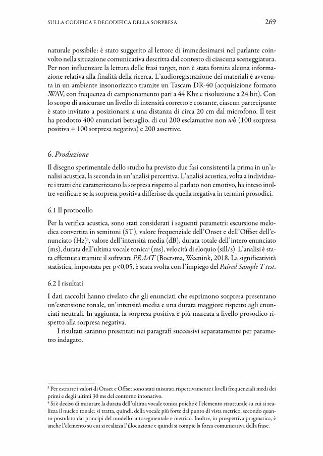
SULLA CODIFICA E DECODIFICA DELLA SORPRESA 269
naturale possibile: è stato suggerito al lettore di immedesimarsi nel parlante coin-volto nella situazione comunicativa descritta dal contesto di ciascuna sceneggiatura. Per non influenzare la lettura delle frasi target, non è stata fornita alcuna informa-zione relativa alla finalità della ricerca. L’audioregistrazione dei materiali è avvenu-ta in un ambiente insonorizzato tramite un Tascam DR-40 (acquisizione formato .WAV, con frequenza di campionamento pari a 44 Khz e risoluzione a 24 bit). Con lo scopo di assicurare un livello di intensità corretto e costante, ciascun partecipante è stato invitato a posizionarsi a una distanza di circa 20 cm dal microfono. Il test ha prodotto 400 enunciati bersaglio, di cui 200 esclamative non wh (100 sorpresa positiva + 100 sorpresa negativa) e 200 assertive.
6. ProduzioneIl disegno sperimentale dello studio ha previsto due fasi consistenti la prima in un’a-nalisi acustica, la seconda in un’analisi percettiva. L’analisi acustica, volta a individua-re i tratti che caratterizzano la sorpresa rispetto al parlato non emotivo, ha inteso inol-tre verificare se la sorpresa positiva differisse da quella negativa in termini prosodici.
6.1 Il protocollo
Per la verifica acustica, sono stati considerati i seguenti parametri: escursione melo-dica convertita in semitoni (ST), valore frequenziale dell’Onset e dell’Offset dell’e-nunciato (Hz)3, valore dell’intensità media (dB), durata totale dell’intero enunciato (ms), durata dell’ultima vocale tonica4 (ms), velocità di eloquio (sill/s). L’analisi è sta-ta effettuata tramite il software PRAAT (Boersma, Weenink, 2018. La significatività statistica, impostata per p<0,05, è stata svolta con l’impiego del Paired Sample T test.
6.2 I risultati
I dati raccolti hanno rivelato che gli enunciati che esprimono sorpresa presentano un’estensione tonale, un’intensità media e una durata maggiore rispetto agli enun-ciati neutrali. In aggiunta, la sorpresa positiva è più marcata a livello prosodico ri-spetto alla sorpresa negativa.
I risultati saranno presentati nei paragrafi successivi separatamente per parame-tro indagato.
3 Per estrarre i valori di Onset e Offset sono stati misurati rispettivamente i livelli frequenziali medi dei primi e degli ultimi 30 ms del contorno intonativo.4 Si è deciso di misurare la durata dell’ultima vocale tonica poiché è l’elemento strutturale su cui si rea-lizza il nucleo tonale: si tratta, quindi, della vocale più forte dal punto di vista metrico, secondo quan-to postulato dai principi del modello autosegmentale e metrico. Inoltre, in prospettiva pragmatica, è anche l’elemento su cui si realizza l’illocuzione e quindi si compie la forza comunicativa della frase.
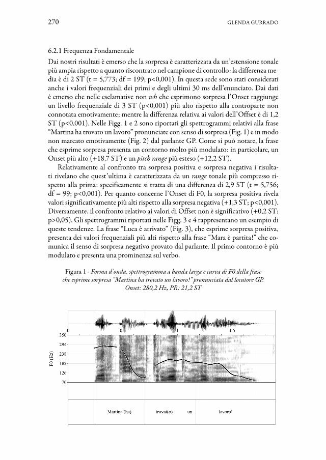
270 GLENDA GURRADO
6.2.1 Frequenza FondamentaleDai nostri risultati è emerso che la sorpresa è caratterizzata da un’estensione tonale più ampia rispetto a quanto riscontrato nel campione di controllo: la differenza me-dia è di 2 ST (t = 5,773; df = 199; p<0,001). In questa sede sono stati considerati anche i valori frequenziali dei primi e degli ultimi 30 ms dell’enunciato. Dai dati è emerso che nelle esclamative non wh che esprimono sorpresa l’Onset raggiunge un livello frequenziale di 3 ST (p<0,001) più alto rispetto alla controparte non connotata emotivamente; mentre la differenza relativa ai valori dell’Offset è di 1,2 ST (p<0,001). Nelle Figg. 1 e 2 sono riportati gli spettrogrammi relativi alla frase “Martina ha trovato un lavoro” pronunciate con senso di sorpresa (Fig. 1) e in modo non marcato emotivamente (Fig. 2) dal parlante GP. Come si può notare, la frase che esprime sorpresa presenta un contorno molto più modulato: in particolare, un Onset più alto (+18,7 ST) e un pitch range più esteso (+12,2 ST).
Relativamente al confronto tra sorpresa positiva e sorpresa negativa i risulta-ti rivelano che quest’ultima è caratterizzata da un range tonale più compresso ri-spetto alla prima: specificamente si tratta di una differenza di 2,9 ST (t = 5,756; df = 99; p<0,001). Per quanto concerne l’Onset di F0, la sorpresa positiva rivela valori significativamente più alti rispetto alla sorpresa negativa (+1,3 ST; p<0,001). Diversamente, il confronto relativo ai valori di Offset non è significativo (+0,2 ST; p>0,05). Gli spettrogrammi riportati nelle Figg. 3 e 4 rappresentano un esempio di queste tendenze. La frase “Luca è arrivato” (Fig. 3), che esprime sorpresa positiva, presenta dei valori frequenziali più alti rispetto alla frase “Mara è partita!” che co-munica il senso di sorpresa negativo provato dal parlante. Il primo contorno è più modulato e presenta una prominenza sul verbo.
Figura 1 - Forma d’onda, spettrogramma a banda larga e curva di F0 della frase che esprime sorpresa “Martina ha trovato un lavoro!” pronunciata dal locutore GP.
Onset: 280,2 Hz, PR: 21,2 ST

SULLA CODIFICA E DECODIFICA DELLA SORPRESA 271
Figura 2 - Forma d’onda, spettrogramma a banda larga e curva di F0 della frase non connotata emotivamente “Martina ha trovato un lavoro.” pronunciata dal locutore GP.
Onset: 94,7 Hz, PR: 9 ST
Figura 3 - Forma d’onda, spettrogramma a banda larga e curva di F0 della frase che esprime sorpresa positiva “Luca è arrivato!” pronunciata dal locutore GP. Onset:
245,4 Hz, PR: 21,6 ST

272 GLENDA GURRADO
Figura 4 - Forma d’onda, spettrogramma a banda larga e curva di F0 della frase che esprime sorpresa negativa “Mara è partita!” pronunciata dal locutore GP. Onset:
157,2 Hz, PR: 11,3 ST
6.2.2 IntensitàGli enunciati che comunicano sorpresa sono anche più intensi rispetto agli enun-ciati non emotivi. Come si può notare dal boxplot in Fig. 5, si rileva una differenza significativa di 3,9 dB (t = 12,991; df = 199; p<0,01).
Figura 5 - Intensità media (dB) delle frasi che esprimono sorpresa e di quelle non connotate emotivamente

SULLA CODIFICA E DECODIFICA DELLA SORPRESA 273
La sorpresa positiva rivela un’intensità media maggiore rispetto alla sorpresa negati-va (+2 dB, t = 3,755; df = 99; p<0,001), come riportato nel boxplot in Fig. 6.
Figura 6 - Intensità media (dB) delle frasi che esprimono sorpresa positiva e di quelle che comunicano sorpresa negativa
6.2.3 DurataRelativamente a questo parametro abbiamo registrato sia la durata totale dell’inte-ro enunciato che la durata dell’ultima vocale tonica. La sorpresa rivela una durata totale maggiore rispetto al campione di controllo: la differenza fra i due gruppi è di 174,2 ms (t = 12,179; df = 199; p>0,001). La vocale nucleare è invece più lunga di 34,2 ms (t = 11,540; df = 199; p<0,001). Gli enunciati che esprimono sorpresa sono quindi più lenti (-0,8 ms, t = -13,207; df = 199; p<0,001). Nelle Figg. 7 e 8, è possibile notare come la parlante GM pronunci la frase che esprime sorpresa Luca è arrivato! (Fig. 7) allungando la vocale nucleare di circa 80 ms rispetto alla sua con-troparte non connotata emotivamente (Fig. 8).
Relativamente al confronto fra sorpresa positiva e sorpresa negativa, è necessario specificare che le frasi appartenenti ai due gruppi messi a confronto non sono mor-fologicamente e sintatticamente identiche e ciò potrebbe aver inficiato la valutazio-ne delle tendenze temporali. Ciò nonostante, dato che in fase di composizione delle sceneggiature sono state scelte frasi target formate da un numero di costituenti simi-le, è possibile comunque analizzare e confrontare i risultati. I dati hanno mostrato che il parametro della durata non è influenzato dall’attitudine positiva o negativa; in questo caso le differenze fra i due gruppi non sono significative (-55 ms, t = -1,118; df = 99; p>0,05). Relativamente alla durata dell’ultima vocale tonica, si registra una differenza di soli 4,1 ms (t = 0,644; df = 99; p>0,05). Tuttavia, il confronto relativo alla velocità elocutiva è significativo (-0,36, t = -2,599; df = 99; p<0,05).

274 GLENDA GURRADO
Figura 7 - Forma d’onda, spettrogramma a banda larga e curva di F0 della frase che esprime sorpresa “Luca è arrivato!” pronunciata dalla locutrice GM.
DT: 1160 ms, DVT: 224 ms
Figura 8 - Forma d’onda, spettrogramma a banda larga e curva di F0 della frase non connotata emotivamente “Luca è arrivato!” pronunciata dalla locutrice GM.
DT: 1030 ms, DVT: 146 ms
7. PercezioneDai dati raccolti nell’analisi acustica, è emerso che le frasi che esprimono sorpresa pre-sentano un’estensione tonale più ampia, un Onset di F0 più alto, un’intensità mag-giore e un eloquio più lento. Con l’obiettivo di verificare il ruolo svolto da alcuni di questi parametri nella percezione della sorpresa, è stato elaborato un test percettivo.

SULLA CODIFICA E DECODIFICA DELLA SORPRESA 275
7.1 Il protocollo
Il principale obiettivo è quello di comprendere la misura in cui F0 e durata influen-zino il giudizio degli ascoltatori nella percezione del grado di sorpresa provato dal parlante; in particolare, i parametri indagati sono l’Onset di F0 e la durata dell’ul-tima vocale tonica (DVT). In questo caso, si è ipotizzato che all’abbassamento dei valori di questi parametri corrisponda una riduzione del livello di sorpresa per-cepito. L’esperimento ha previsto la manipolazione di un sottocorpus di stimoli preselezionati: due esclamative originali pronunciate dalla parlante CL sono state sottoposte all’abbassamento in tre step dei valori di Onset di F0 e della DVT. Gli enunciati scelti esprimono sorpresa positiva (CL_1T: Luca è arrivato!) e sorpresa negativa (CL_3T: Mara è partita!)5. La manipolazione dei parametri è stata effet-tuata tramite sintesi vocale delle frasi, mediante il sistema PSOLA disponibile nel software PRAAT. Specificamente, il procedimento sperimentale ha comportato: 1) l’accorciamento temporale della vocale nucleare in tre step da 15 ms; 2) l’abbassa-mento frequenziale dei primi 30 ms del contorno (Onset) in tre step da 1,5 ST6. La manipolazione è stata effettuata sia singolarmente che in maniera congiunta. Come si può dedurre dalla Tab. 1, gli stimoli ottenuti sono di sei tipi:
Tabella 1 - Step di manipolazione singola e congiunta degli stimoli audio selezionati
D1 D2 D3-15 ms -30 ms -45 ms
F01 F02 F03-1,5 ST -3 ST -4,5 ST
D1+F01 D2+F02 D3+F03-15 ms -1,5 ST -30 ms -3 ST -45 ms -4,5 ST
Il numero totale degli stimoli ottenuti è 36, organizzati nel seguente modo:– 6 esclamative con manipolazione della DVT;– 6 esclamative con manipolazione dell’Onset;– 6 esclamative con manipolazione congiunta di DVT e Onset;– 18 filler7.
5 Questi enunciati sono stati selezionati in seguito a un pre-test in cui è stato chiesto a un gruppo ri-stretto di ascoltatori di giudicare, tramite scala Likert a 7 punti, il grado di sorpresa comunicato da una serie di frasi. Le esclamative CL_1T e CL_3T comparivano fra quelle che avevano raggiunto i pun-teggi più alti. La frase CL_1T (Luca è arrivato!) è accompagnata da un contesto che descrive l’arrivo ad una festa di Luca, un caro amico del parlante, si tratta quindi di un evento gradito. La situazione in cui è pronunciata CL_3T (Mara è partita!) è, invece, sgradita, poiché l’amica Mara è partita improv-visamente senza avvisare.6 I valori acustici degli stimoli hanno dettato la scelta degli step: la media della differenza fra l’Onset e la DVT delle frasi che esprimono sorpresa da un lato e l’Onset e la DVT delle frasi non marcate emotivamente dall’altro è rispettivamente di circa 4 ST e 40 ms.7 I filler consistono in frasi appartenenti a modalità frasali diverse da quella esclamativa, nello specifico assertive e interrogative non connotate emotivamente.

276 GLENDA GURRADO
Gli stimoli ottenuti dalla sintesi, unitamente agli originali e ai filler, sono stati proposti in via telematica e in ordine randomizzato a un gruppo di 35 studentesse dell’Università degli Studi di Bari (età media 23,5 anni), nate e cresciute in area Apulo-Barese. Per ciascun enunciato si chiedeva “Secondo te la frase ascoltata espri-me sorpresa?”; le partecipanti sono state quindi invitate a valutare il grado di sorpre-sa espresso tramite una scala Likert a 5 punti da “Per nulla” (1) a “Moltissimo” (5). Agli informatori non sono state fornite indicazioni circa le finalità della ricerca, allo scopo di non influenzare le loro risposte nel test.
7.2 I risultati
Da un’analisi preliminare dei punteggi raccolti, fra le due frasi selezionate è emer-sa una certa differenza di giudizi del livello di sorpresa percepito. Come riportato nella Tab. 2, i punteggi differiscono significativamente fra i due gruppi per tutti gli stimoli manipolati sia in maniera singola che congiunta. Come si può notare dai risultati, la media dei giudizi relativi alla frase che esprime sorpresa positiva è signi-ficativamente più alta rispetto a quella dei giudizi ottenuti dalla frase che comunica sorpresa negativa. I due enunciati sembrerebbero essere stati, quindi, percepiti dagli ascoltatori con livelli di sorpresa diversi, una tendenza probabilmente connessa alla differenza di valenza dell’emozione convogliata.
Tabella 2 - Confronto statistico fra i punteggi ottenuti da ciascuno stimolo manipolato nei due enunciati CL_1T e CL_3T
Confronto fra stimoli Diff. media t df Sig.
D1_1T – D1_3T 1,17 4,797 34 <0,001D2_1T – D2_3T 1,46 5,166 34 <0,001D3_1T – D3_3T 1,89 7,294 34 <0,001
F01_1T – F01_3T 1,89 6,393 34 <0,001F02_1T – F02_3T 1,57 6,039 34 <0,001F03_1T – F03_3T 1,29 4,410 34 <0,001
D1F01_1T – D1F01_3T 1,37 4,928 34 <0,001D2F02_1T – D2F02_3T 1,11 3,853 34 <0,001D3F03_1T – D3F03_3T 1,74 5,259 34 <0,001
Sulla base dei risultati ottenuti da questa analisi preliminare, al fine di comprendere se i giudizi dei parlanti siano influenzati dalla manipolazione dei parametri, i pun-teggi sono stati sottoposti all’analisi statistica tramite Friedman test8 separatamente per enunciato. L’analisi ha rivelato che gli stimoli manipolati non differiscono in
8 Il Friedman test è la versione non parametrica del one-way ANOVA with repeated measures. Si tratta di un modello impiegato per testare la differenza fra gruppi nei casi in cui la variabile dipendente sia ordinale. Solitamente, il Friedman test è impiegato anche quando non siano rispettati i presupposti ne-cessari allo svolgimento del modello parametrico corrispondente. Nel nostro caso, la scelta è ricaduta su questo test poiché la variabile in esame è tendenzialmente riconosciuta come ordinale (si tratta dei punteggi ricavati dalla scala Likert utilizzata dai partecipanti al test percettivo).

SULLA CODIFICA E DECODIFICA DELLA SORPRESA 277
modo statisticamente significativo in termini di livello di sorpresa percepito9, né in riferimento alla frase 1T (X2(8) = 9,202, p>0,05), né a quella 3T (X2(8) = 11,692, p>0,05); in altre parole, l’abbassamento dei valori di Onset e l’accorciamento della DVT non hanno comportato una relativa diminuzione del livello di sorpresa per-cepito. I line plot riportati nelle Figg. 9 e 10 aiutano a comprendere le tendenze. Nel caso di Luca è arrivato! (Fig. 9) il punteggio più basso di sorpresa percepita è stato attribuito al primo step di manipolazione della durata (D1) e agli stimoli di mani-polazione congiunta (D2F02-D3F03). Tale dato non era disatteso: ci si aspettava, infatti, che l’abbassamento congiunto dei valori frequenziali e temporali avrebbe comportato una diminuzione del grado di sorpresa trasmesso. Tuttavia, alcune ten-denze sono poco chiare, il primo livello di manipolazione della durata, ad esempio, ha ottenuto un SurpriseScore più basso rispetto agli altri stimoli. In particolare, ri-sulta inatteso il fatto che alle variazioni frequenziali non siano corrisposti abbassa-menti nei giudizi.
Figura 9 - Line plot del SurpriseScore attribuito alle sette categorie di stimoli per la frase “Luca è arrivato” (CL_1T)
Passiamo ad analizzare il lineplot dei punteggi raccolti per la frase Mara è partita! (Fig. 10).
9 Da qui in poi il punteggio attribuito dagli uditori al livello di sorpresa percepito sarà definito SurpriseScore.

278 GLENDA GURRADO
Figura 10 - Line plot del SurpriseScore attribuito alle sette categorie di stimoli per la frase “Mara è partita!” (CL_3T)
Come è stato anticipato, il confronto non è supportato da significatività statisti-ca, alcune tendenze, però, sono interessanti: a una maggiore riduzione della durata sembra corrispondere un indebolimento del senso di sorpresa trasmesso. Allo stesso modo, un abbassamento interessante si rileva in corrispondenza della manipolazio-ne congiunta D3F03. Il quadro più particolare è quello relativo alla manipolazione dell’Onset di F0: seppure in modo non significativo abbiamo un lieve innalzamento del senso di sorpresa percepito nel passaggio dal primo al terzo test di manipolazione.
8. Discussione e conclusioniL’attenzione finora rivolta alla prosodia delle espressioni di sorpresa si è concentrata in pochi studi dedicati alla codifica e alla decodifica delle emozioni base. Ciò può essere, presumibilmente, ricondotto a due principali motivazioni. In primis, secon-do alcuni studiosi la sorpresa tende a essere comunicata principalmente mediante espressioni facciali; è probabile che tale aspetto renda più ostica un’analisi fonetica dei parametri prosodici che caratterizzano questa emozione sia in produzione che in percezione. Inoltre, i confini tra la sorpresa e le altre emozioni sono spesso sfumati: la sorpresa in alcuni contesti può, infatti, sfociare nella gioia o, diversamente, nella rabbia. Si tratta quindi di un’emozione base poco indagata a livello acustico e ancor meno osservata separatamente in relazione alle diverse valenze che la caratterizzano e che in questa sede abbiamo voluto mettere sotto esame, analizzando la modalità frasale che per definizione dovrebbe veicolarla.
Dagli studi condotti fino ad oggi, è emerso che questa emozione sarebbe contrad-distinta da alti valori di F0, un’estensione tonale ampia, un’intensità alta, un eloquio veloce e quindi una riduzione del numero di pause. Si tratta di un quadro prosodico che secondo l’approccio dimensionale farebbe rientrare la sorpresa fra le emozioni

SULLA CODIFICA E DECODIFICA DELLA SORPRESA 279
ad alta attivazione. Tuttavia, come sappiamo, con riferimento alla dimensione della valutazione, le emozioni con connotazione positiva si oppongono a emozioni con connotazione negativa. Ci si è chiesti, dunque, se esistano delle differenze fra sor-presa positiva e sorpresa negativa a livello prosodico. L’intento di verificare le carat-teristiche intonative delle espressioni di sorpresa si scontra, quindi, con queste pre-messe e con le numerose variabili che possono presentarsi in un contesto che, come è ovvio, può deviare da una situazione standard. I risultati del presente studio vanno quindi valutati con cautela. Secondo quanto emerge dalla verifica dei dati, la nostra ricerca ha messo in luce che la sorpresa è caratterizzata dall’attivazione dei parametri di frequenza e durata: questa emozione è infatti contraddistinta da valori di F0 più alti e da un’estensione tonale più ampia. In questo caso, il nostro studio si allinea a quanto riscontrato nei contributi che finora hanno dedicato la loro attenzione alla comunicazione vocale della sorpresa (tra gli altri, Cahn, 1990; Abelin, Allwood, 2000; Iriondo et al., 2000; De Marco, Paone, 2014; Maffia et al., 2014). Per quanto concerne il parametro della durata, i nostri dati si discostano dalla tendenza riscon-trata in questi contributi, dai quali emerge una sorpresa caratterizzata da un eloquio veloce, per allinearsi con i risultati di Abelin, Allwood (2000) riferiti al tedesco, in cui nella sorpresa si riscontra una durata maggiore rispetto al parlato neutrale. Nella nostra indagine, si è, inoltre, rivolta l’attenzione al confronto fra sorpresa positiva e negativa. In questo caso è emerso che la sorpresa positiva è più intensa e presenta un’estensione tonale più ampia rispetto alla sorpresa negativa. Gli enunciati che co-municano sorpresa positiva sono, quindi, caratterizzati sul piano prosodico da quegli indici fonetici che nelle ricerche finora eseguite sono stati associati all’espressione della sorpresa, tali aspetti sono, però, meno marcati negli enunciati che comunicano sorpresa negativa. Questo quadro ci suggerisce quanto ancora poco si conosca sul li-vello soprasegmentale di alcune espressioni connesse alle emozioni primarie e quanto la variabilità derivante dal contesto possa influire sulle sfaccettature delle stesse.
Tale dato ha quindi posto l’accento sul fatto che anche per la sorpresa è necessario considerare le diverse sfumature emotive. Scherer (2003) parla di famiglie di emozio-ni, si distingue ad esempio fra exuberant joy e quite happiness, oppure fra hot e cold anger, sostenendo che, in alcuni contesti, i membri di una stessa famiglia emotiva si differenzino significativamente a livello vocale. Anche la sorpresa può, probabilmen-te, avere varie anime, a seconda della forza con cui l’evento inaspettato colpisca emo-tivamente il parlante. Oltre a ciò si ha un’ulteriore dicotomia tra sorpresa positiva e sorpresa negativa, declinazioni legate alla portata piacevole o spiacevole dell’evento e della notizia inaspettata che stimola la reazione emotiva. La nostra riflessione, però, prosegue traendo spunto anche da alcune criticità rilevate in altri test percettivi volti all’identificazione e al corretto riconoscimento delle emozioni. Un evento inaspetta-to suscita sorpresa nel parlante, tuttavia nell’espressione emotiva i confini fra le varie emozioni possono essere sfumati: il soggetto può essere sorpreso ma se l’evento che ha scatenato tale emozione è particolarmente gradito si può sfociare nella gioia o, in caso diverso, nella rabbia. Da questo sfrangiamento dei contorni deriva anche la dif-ficoltà negli studi sperimentali basati sul metodo della simulated emotional expression

280 GLENDA GURRADO
nel calibrare perfettamente la sceneggiatura che possa stimolare una reazione di pura sorpresa nel parlante. Quindi ci si chiede cosa succede a livello prosodico quando un’emozione è ibrida: poiché è vero che le emozioni ad alta attivazione condividono una prosodia contraddistinta dall’innalzamento di una serie di parametri, ma diversi studi ci suggeriscono che esse si distinguono per alcuni aspetti. Partendo da questo presupposto sarebbe interessante capire cosa accade a livello prosodico quando si in-nesca uno sconfinamento del perimetro che contorna ciascuna emozione.
Per quanto concerne la percezione, nella nostra ricerca non si è voluto indagare le modalità di riconoscimento o di identificazione delle emozioni. Si è inteso, in-fatti, osservare la misura in cui alcuni parametri prosodici influenzano il livello di sorpresa percepito dagli uditori. Si è ipotizzato che esistano diversi gradi di sorpresa che un soggetto può provare e si è voluto, quindi, verificare se la manipolazione di alcuni parametri possa influenzare tale percezione determinando una variazione nel livello dell’emozione decodificata.
Il nostro studio ci suggerisce da un lato che l’abbassamento dei valori dell’Onset di F0 e della durata dell’ultima vocale tonica non comportano un indebolimento del grado di sorpresa trasmesso, dall’altro ci mostrano delle tendenze di difficile let-tura e che meritano di essere chiarite, probabilmente mediante la ripetizione del test sottoponendolo a un campione più numeroso, valutando, inoltre, altri parametri probabilmente coinvolti in misura maggiore in questo processo.
Un altro aspetto su cui occorrerebbe concentrarsi in futuro sono le modalità di percezione della sorpresa in base alla connotazione affettiva della stessa, quindi sorpresa positiva e negativa. Dai nostri risultati, infatti, i giudizi espressi per i due enunciati selezionati differiscono significativamente: la frase che esprime sorpresa positiva, indifferentemente dal tipo di manipolazione, ha ottenuto punteggi supe-riori rispetto alla frase che comunica sorpresa negativa; in altri termini, i parlanti hanno percepito una differenza nel livello di sorpresa provato dal parlante. Tale ten-denza merita di essere ulteriormente approfondita.
È importante sottolineare, infine, che il disegno sperimentale ha previsto l’analisi di parlato semirecitato. La questione relativa alla modalità di elicitazione degli sti-moli più adatta all’analisi della comunicazione delle emozioni è stata a lungo dibat-tuta (es. Russell, 1994), in particolare, ci si è chiesti se il parlato letto potesse essere rappresentativo dell’espressione spontanea delle emozioni. Secondo Scherer (2003) ogni modalità di elicitazione dello stato emotivo dello speaker può comportare delle problematiche. L’autore suggerisce che la simulated vocal expression (che dovrebbe coinvolgere dei parlanti che abbiano delle esperienze attoriali anche minime) sareb-be il metodo di elicitazione delle emozioni più utilizzato in questo filone di studi. Tuttavia, secondo la prospettiva di Scherer non si può escludere che gli attori esageri-no volutamente alcuni aspetti, minimizzandone degli altri: in altre parole potrebbe-ro essere influenzati dagli stereotipi legati al parlato emotivo. Ciononostante, il fatto che i vocal portrayals siano decodificati correttamente dagli ascoltatori suggerirebbe che il parlato controllato probabilmente rispecchia le caratteristiche acustiche del parlato emotivo naturale. Secondo alcuni autori, il parlato emotivo simulato (emo-

SULLA CODIFICA E DECODIFICA DELLA SORPRESA 281
tional portayals), basandosi su espressioni naturali, dovrebbe condividerne le carat-teristiche acustiche (Banse, Scherer, 1996; Juslin, Laukka, 2003), pensiero sostenu-to anche da Pell et al. (2009). Tuttavia, studi più recenti, come quello di Dhamyal, Memon, Raj & Singh (2019), rivelano una differenza significativa tra parlato reci-tato e parlato spontaneo a livello fonetico, suggerendo di optare per il secondo, in quanto ritenuto più valido e affidabile nello studio della comunicazione emotiva.
Nel caso del presente lavoro si è preferito un parlato letto, basato su delle sce-neggiature preconfezionate contenenti le frasi target che, in riferimento al contesto, dovrebbero veicolare l’emozione sorpresa del parlante. Questa scelta è stata effettua-ta con riferimento alla prospettiva degli studi degli autori citati nonché sulla base dell’intenzione di attuare una comparazione diretta e sistematica tra enunciati identi-ci per struttura sintattica e morfologica e ottenere, dunque, dei dati fonetici e prosodi-ci confrontabili. Nel nostro caso, invitando a partecipare alla sessione di registrazione dei parlanti che non avessero esperienze attoriali, si è inoltre cercato di evitare la possi-bilità di incorrere nell’eccessiva enfatizzazione della produzione del parlato emotivo.
Tuttavia, consapevoli che l’utilizzo di un parlato ecologicamente valido sia utile e necessario all’indagine delle caratteristiche del parlato emotivo, ci si riserva di spa-ziare nello studio della sorpresa in questo senso in uno studio futuro.
Riferimenti bibliografici
Abelin, Å., Allwood, J. (2000). Cross linguistic interpretation of emotional prosody. In ISCA Tutorial and Research Workshop (ITRW) on Speech and Emotion, Newcastle, UK, 5-7 September 2000, 110-113.Banse, R., Scherer, K.R. (1996). Acoustic profiles in vocal emotion expression. In Journal of Personality and Social Psychology, 70(3), 614-636. https://doi.org/10.1037//0022-3514.70.3.614Belin, P., Fillion-Bilodeau, S. & Gosselin, F. (2008). The MontrealAffective Voices: A validated set of nonverbal affect bursts for re Behavior Research search on auditory af-fective processing. In Behavior research methods, 40(2), 531-539. https://doi.org/10.3758/brm.40.2.531Boersma, P., Weenink, D. (2018). Praat: doing phonetics by computer [Computer pro-gram]. Version 6.0.43, retrieved September, 08 2018 from http://www.praat.org/.Cahn, J.E. (1990). The generation of affect in synthesized speech. In Journal of the American Voice I/O Society, 8, 1-19.Darwin, C. (1872). The expression of emotions in man and animals. Londra: John Murray. [Trad. it.: Ferrari G.A. (a cura di) (1982). L’espressione delle emozioni negli uomini e negli animali. Torino: Boringhieri].De Marco, A., Paone, E. (2014). L’espressione e la percezione delle emozioni vocali in ap-prendenti di Italiano L2. Uno studio cross-linguistico. In Educazione linguistica. Language education, 3, 483-500. http://doi.org/10.14277/2280-6792/339Dhamyal, H., Memon, S.A., Raj, B. & Singh, R. (2020). The phonetic bases of vocal expressed emotion: natural versus acted. In ArXiv. https://arxiv.org/abs/1911.05733v3

282 GLENDA GURRADO
Ekman, P. (2003). Emotions Revealed. Understanding faces and feelings. London: Weidenfeld and Nicolson.Iriondo, I., Guaus, R., Rodríguez, A., Lázaro, P., Montoya, N., Blanco, J.M., Bernadas, D., Oliver, J.M., Tena, D. & Longhi, L. (2000). Validation of an Acoustical Modelling of Emotional Expression in Spanish using Speech Synthesis Techniques. In ISCA Tutorial and Research Workshop (ITRW) on Speech and Emotion, Newcastle, UK, 5-7 September 2000, 161-166.Izard, C.E. (1994). Innate and Universal Facial Expression: Evidence From Developmental and Cross-Cultural Research. In Psychological Bulletin, 115(2), 288-299. https://doi.org/10.1037/0033-2909.115.2.288Gili Fivela B. (2015). L’integrazione di informazioni multimodali: prosodia ed espres-sioni del volto nella percezione del parlato. In Pistolesi E., Pugliese R. & Gili Fivela B. (a cura di), Parole, gesti, interpretazioni. Studi linguistici per Carla Bazzanella. Roma: Aracne, 107-127.Johnstone, T., Scherer, K.R. (2000). Vocal communication of emotions. In Lewis, M., Haviland, J. (Eds.), The handbook of emotions. New York: Guilford, 226-235.Juslin, P.N., Laukka, P. (2003). Communication of emotions in vocal expression and mu-sic performance: Different channels, same code?. In Psychological Bulletin, 129(5), 770-814. https://doi.org/10.1037/0033-2909.129.5.770Maffia, M., Pellegrino, E. & Pettorino, M. (2014). Labelling expressive speech in L2 Italian: The role of prosody in auto-and external annotation. In Campbell, A.W., Gibbon, D. & Hirst, D. (Eds.), Proceedings of the 7th International Conference on Speech Prosody, Dublin, Ireland, 20-23 May 2014, 81-84.Pell, M.D., Paulmann, S., Dara, C., Alasseri, A. & Kotz, S.A. (2009). Factors in the recognition of vocally expressed emotions: A comparison of four languages. In Journal of Phonetics, 37, 417-435. https://doi.org/10.1016/j.wocn.2009.07.005Russell, J.A. (1994). Is there universal recognition of emotion from facial expression? A review of the cross-cultural studies. In Psychological Bulletin, 115(1), 102-41. https://doi.org/10.1037/0033-2909.115.1.102Scherer, K.R. (1989). Vocal correlates of emotional arousal and affective disturbance. In Wagner, H., Manstead, A. (Eds.), Handbook of Psychophysiology: Emotion and social behavior. London: Wiley, 165-197.Scherer, K.R. (2000). Psychological models of emotion. In Borod, J. (Ed.), The Neuropsychology of Emotion. Oxford: Oxford University Press, 137-162.Scherer, K.R. (2003). Vocal communication of emotion: a review of research para-digms. In Speech communication, 40 (1-2), 227-256. https://doi.org/10.1016/S0167-6393(02)00084-5Tomkins, S. (1962). Affect Imagery Consciousness: Volume I, The Positive Affects. London: Tavistock. https://doi.org/10.1037/14351-000Tomkins, S. (1963). Affect Imagery Consciousness: Volume II, The Negative Affects. London: Tavistock.Wundt, W. (1874/1905). Grundzüge der physiologischen Psychologie. Fundamentals of physiological psychology, orig. pub. 1874 fifth ed. Engelmann, Leipzig.

DOI: 10.17469/O2108AISV000015
VALENTINA DE IACOVO, MARCO PALENA, ANTONIO ROMANO
Evaluating prosodic cues in Italian: the use of a Telegram chatbot as a CALL tool for Italian L2 learners
Comparing the pronunciation of learners of a foreign language (FL) with utterances of native speakers is receiving attention thanks to the increasing number of applications arising in the field of computer-assisted teaching (Cazade, 1999) and computer-assisted language learning (Levy, 1997). At the same time, language-learning studies on prosodic inter-speaker variation bring to light a rhythmic-intonational variability that should not be reduced to few acceptable patterns but be part of the learner’s linguistic background. It still seems open to debate how best to make explicit to the learner his degree of prosodic competence on the basis of acoustic features (f0, intensity, duration) and other correlates (syllables, lexical accent, speech rate, pauses). In this study we present a chatbot as a proactive learning support to improve the oral skills in Italian L2.
Keywords: L2 intonation, Italian prosody, oral production, CALL, educational chatbot.
1. IntroductionThe prosodic features of speech reveal important information such as the enunciative mode, the speaking style, the attitude and the regional or social connotations of the speaker, and are therefore essential for successful interpersonal communication (Hirst, 1983; Cruttenden, 1986). However, in many contexts related to foreign language teaching (FL), metaprosodic reflection is not always satisfactory for the learner because it is not dealt with comprehensively. Referring to the role played by prosodic features such as intonation, rhythm, duration, and focus to explain communicative differences in meaning may instead prove indispensable in triggering an awareness in the learner in recognising and reproducing FL speech (Cresti, 1999; Chun, 2002; Frost, Picavet, 2014). Moreover, for several decades now, technological developments in speech analysis have opened the way to new perspectives on communicative interaction that can be used in language teaching (Chun, 1998; Cazade, 1999; Busà, 2012; Romano, Giordano, 2017), and have also led to the emergence, from the very first studies conducted, of criticism towards possible solutions for the explanation of the degree of competence achieved, for example through the use of graphic representations ( James, 1976; De Bot, 1983; Martin, 2010). The teaching of oral FL allows just that kind of metaprosodic reflection (Trouvain, Gut, 2007) thanks to which students can experiment the variety of enunciative combinations and associate their meaning on the basis of specific functions (modal, syntactic, informative, emotional) in order to refine their oral communication skills (Delattre, 1966; Cresti, 1999; De Iacovo, Romano, 2019).

284 VALENTINA DE IACOVO, MARCO PALENA, ANTONIO ROMANO
In Italian it is also necessary to take into account the different intonational choices on the basis of the regional or local variety used (Canepari, 1983, 1985; Bertinetto, Magno Caldognetto, 1993; Sorianello, 2006) included for some time now in the research on L2 intonation (De Meo, Pettorino, 2012; De Marco, Sorianello & Mascherpa, 2014) that allows the learner a greater choice among prosodic models. Finally, we find it interesting to focus on the different possibilities of realization typical of oral language and how they should be taken into account in the context of automatic evaluation and recurrence of intonation patterns.
On the basis of these considerations, our work is structured as follows: after setting up the chatbot’s steps for prosodic evaluation, we recorded a set of ten complex sentences constructed to give an adequate representation of the most frequent intonational solutions of a formal speech on technical-scientific contents, but also including some everyday expressions by native Italian speakers to be used as a comparison with Italian learners. The results obtained thanks to the comparison between the sentences produced by Italian speakers and learners thus provide a first cue to reflecting on some considerations that have emerged: in what way do the values of the acoustic parameters extracted by the chatbot reflect a perceptual evaluation? (Munro, Derwing, 1999) What are the most recurrent prosodic patterns used by Italian speakers and students? What is the degree of reliability of the automatic segmentation system with respect to the results returned? (Lacheret-Dujour, 2001).
2. Chatbot structure and functioningIn this section we illustrate how the chatbot has been structured as an assisted teaching tool for the assessment of prosodic features. The adoption of such an instrument has several advantages. First of all, it provides a text-based mode of interaction to which the public is already largely accustomed thanks to the popularity of instant messaging applications such as Whatsapp or Telegram. This makes these tools easier to use than dedicated applications or Learning Management Systems (LMS) such as Moodle or Blackboard, whose main obstacle to usability is the need for users to adapt to an unfamiliar interface. Moreover, a chatbot allows for interaction with learners in a structured and asynchronous way: structured because it is organised according to predefined schemes, aimed at reducing ambiguities; asynchronous because it is not bound to continuous time intervals but can be used freely according to one’s own time availability. The potential of chatbots as teaching aids has been investigated for a few years now (Pereira, 2016; Fernoagă, Stelea, Gavrilă & Sandu, 2018) and several recent studies have focussed on their pedagogical (Cheng, Lau, Lam, Zhan & Chan, 2020) and prosodic assessment (Lezhenin, Lamtev, Dyachkov, Boitsova, Vylegzhanina & Bogach, 2017).
Implemented within the instant messaging application Telegram, the chatbot (or bot) developed involves interaction with the user through questions and answers based on the assessment of technical knowledge. In particular, it directs to the learner a series of closed-ended questions (quizzes) that can be of a general nature

EVALUATING PROSODIC CUES IN ITALIAN 285
of linguistic comprehension or linked to a particular subject area (e.g. technical or scientific). When the correct answer is found, the learner sends a statement of the answer by voice message. The received utterance is then automatically processed by the bot in order to obtain an evaluation of the intonation level of the speaker. This processing can be summarised in the following steps:1. Pre-processing2. Phonetic segmentation3. Extraction of fundamental frequency values4. Intonation analysisThe first step in the processing chain has a dual purpose: to guarantee a minimum quality level for the input audio signal and to prepare it for further processing. The audio is first converted to single-channel wav format, resampled (if necessary) to 48 kHz and cleaned of background noise. The average amplitude value and signal-to-noise ratio of the resulting audio are then estimated. If the estimated values are below certain predefined thresholds, the chatbot prompts the learner to record a new utterance in a less noisy environment and/or by speaking in a higher tone of voice. The speech signal is then subjected to segmentation using the WebMAUS Basic web service (Kisler, Reichel & Schiel, 2018). This service, taking as input the speech signal and the orthographic transcription of the utterance, returns a segmentation into words and phonemes based on the method described in Schiel (1999). The phonetic segmentation of the utterance, provided in TextGrid format to facilitate subsequent processing using Praat software (Boersma, Weenink, 2018), is then processed by labelling individual phonemes as vowels or consonants (Fig. 1). A Praat script is then invoked to extract the fundamental frequency (f0) values of the previously identified vowel phonemes, thus obtaining the intonation curve of the utterance (for the segmentation and value extraction model, see Romano, Contini & Lai, 2014).
Figure 1 - Praat screen (wav and Textgrid) showing the phonetic segmentation made by WebMaus for the utterance “Non avere nessuna possibilità di agire come si vorrebbe”

286 VALENTINA DE IACOVO, MARCO PALENA, ANTONIO ROMANO
The analysis of intonation is carried out by comparing the intonational curve of the learner’s utterance with the f0 traces of the corresponding utterances of native speakers, previously collected and evaluated using the same automatic procedure. The comparison is made by calculating a correlation measure (Moutinho de Castro, Coimbra, Rilliard & Romano, 2011) that compares for each sentence three points (initial, central, final) of f0 of each vowel segment identified by Maus. Such a measure is known as the Pearson correlation coefficient:
(1)
where X and Y are two data series of n values each, corresponding to the f0 traces, the values μX and μY represent the means of these data series and the values X and σY represent their standard deviations. The Pearson coefficient is a measure of linear correlation and its value ranges between -1 and 1 (or in percentage between -100% and 100%). A positive value indicates linear correlation between the two data series, meaning that most pairs of f0 values tend to be simultaneously greater than, or simultaneously less than, their respective means. A value of 1 indicates perfect linear correlation, meaning that each pair f0 values increases or decreases accordingly and always with the same proportions. Conversely, a negative value indicates anti-correlation, meaning that the pairs of f0 values tend to lie on opposite sides of their respective means. A value of -1 indicates perfect anti-correlation, meaning that for each pair of f0 values, as one increases the other decreases and always with the same proportions. A value of 0 implies that there is no linear correlation between the two data series.
Due to the extemporaneous nature of the recorded speech signals and the automatic mode of the segmentation procedure operated by Maus, the vocalic segments detected for learners’ utterances and those detected for the corresponding utterances of native speakers might differ. Therefore, before calculating the correlation, the segments of the two speakers are aligned on the basis of both the phonetic information they contain and their temporal position (Fig. 2). The correlation measure is then restricted to all and only those vowel segments to ensure phonetic-segmental homogeneity between the two speakers.

EVALUATING PROSODIC CUES IN ITALIAN 287
Figure 2 - Segmented audio, temporal alignment and segment matching
The administration of the task (Fig. 3) foresees a first registration phase in which the user indicates some of his sociolinguistic data (the linguistic level according to the CEFR, if and where he has lived in Italy, in which contexts he is used to speak Italian). Subsequently, after a microphone test demonstrating sufficient audio quality, the user can begin the task: each question is presented in written and oral form while the choice of the answer is among four options (see Appendix for the complete list of sentences).
Figure 3 - Screenshots showing the main steps of the interaction chatbot-user

288 VALENTINA DE IACOVO, MARCO PALENA, ANTONIO ROMANO
If the user provides the wrong answer, he can try again and, once the correct answer is chosen, the chatbot suggests to record the answer through an audio message. At this point of the interaction, the elicited sentence is compared with those in the database and, after identifying the one with the highest intonation closeness, the chatbot returns the correlation value in percentage form. At the end of the task, a summary score obtained from the average of the values for each answer is calculated.
3. Collected data and some first resultsA comparison with data from native speakers has been undertaken for several years (Delmonte, 2009) and deals well with the new ways of assessing automatic speech recognition systems. In this first phase of the project, we created a set of 10 questions and answers. Numbers, dates and medium complex intonation structures1 (listed in the appendix) were included in the answer, which represents the comparison sentence, in order to have utterances of medium-high reading difficulty. The set was then read by 250 people who recorded question and answer using a mobile phone device leading to the creation of a database of 2500 sentences. The audio was then resampled to 16 kHz and, through manual segmentation, only the answers were segmented and labelled. The recorded samples came from different parts of Italy (half from Piedmont) and include 164 females and 84 males aged between 15
1 This refers to a sentence with more than one intonation units (declarative, interrogative, continuative).
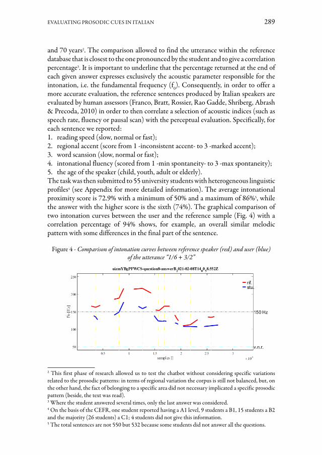
EVALUATING PROSODIC CUES IN ITALIAN 289
and 70 years2. The comparison allowed to find the utterance within the reference database that is closest to the one pronounced by the student and to give a correlation percentage3. It is important to underline that the percentage returned at the end of each given answer expresses exclusively the acoustic parameter responsible for the intonation, i.e. the fundamental frequency (f0). Consequently, in order to offer a more accurate evaluation, the reference sentences produced by Italian speakers are evaluated by human assessors (Franco, Bratt, Rossier, Rao Gadde, Shriberg, Abrash & Precoda, 2010) in order to then correlate a selection of acoustic indices (such as speech rate, fluency or pausal scan) with the perceptual evaluation. Specifically, for each sentence we reported:1. reading speed (slow, normal or fast);2. regional accent (score from 1 -inconsistent accent- to 3 -marked accent);3. word scansion (slow, normal or fast);4. intonational fluency (scored from 1 -min spontaneity- to 3 -max spontaneity);5. the age of the speaker (child, youth, adult or elderly).The task was then submitted to 55 university students with heterogeneous linguistic profiles4 (see Appendix for more detailed information). The average intonational proximity score is 72.9% with a minimum of 50% and a maximum of 86%5, while the answer with the higher score is the sixth (74%). The graphical comparison of two intonation curves between the user and the reference sample (Fig. 4) with a correlation percentage of 94% shows, for example, an overall similar melodic pattern with some differences in the final part of the sentence.
Figure 4 - Comparison of intonation curves between reference speaker (red) and user (blue) of the utterance “1/6 + 3/2”
2 This first phase of research allowed us to test the chatbot without considering specific variations related to the prosodic patterns: in terms of regional variation the corpus is still not balanced, but, on the other hand, the fact of belonging to a specific area did not necessary implicated a specific prosodic pattern (beside, the text was read).3 Where the student answered several times, only the last answer was considered.4 On the basis of the CEFR, one student reported having a A1 level, 9 students a B1, 15 students a B2 and the majority (26 students) a C1; 4 students did not give this information.5 The total sentences are not 550 but 532 because some students did not answer all the questions.

290 VALENTINA DE IACOVO, MARCO PALENA, ANTONIO ROMANO
Figure 5 - Comparison of intonation curves between reference speaker (red) and user (blue) of the utterance “Scusi, ho lasciato l’orologio a casa, sa dirmi che ore sono?”
Even where the fundamental frequency is different (Fig. 5), the correlation allows us to evaluate speakers of different sex (in this case the score is 88%). Other factors such as hesitation within words (as in the example in Fig. 6) may come into play: this kind of phenomenon should be considered for a more coherent overall evaluation of the utterance.
Figure 6 - Praat screen (wav and Textgrid) with the phonetic segmentation performed by WebMaus for the utterance “Se fossi venuto con me, ti avrei portato a mangiare una pizza.”
In a second step, we extracted some specific speech cues (see Tab. 1), in particular:– number of syllables uttered by the speaker out of the duration of each speech-
chain in the sentence (syllable rate, SR)– number of syllables uttered by the speaker out of the total duration of the
sentence (fluency rate, FR)– total duration of pauses in seconds (p. dur.)– number of pauses identified by the automatic segmentation procedure (p.)– number of segments extracted by the automatic segmentation procedure (seg.)– number of syllables extracted by the automatic syllabification procedure (syl.)

EVALUATING PROSODIC CUES IN ITALIAN 291
– number of segments extracted corresponding to vowel phonemes (vow.)– duration of the utterance in seconds (dur.)
The sentences produced by native speakers vary from 2.5 to 4.8 ss while students take on average 1.3 ss longer than native speakers, up to a maximum of 2 ss longer in the first sentence. This sentence is also the one with the highest mean segment gap between native speakers and students (2.9) where on average students tend to add a maximum of 1.7 segments per sentence. The native speaker-student ratio of the number of syllables is between -0.1 (sentence 10) and 0.9 (sentence 1 and 8), with an increase in the number of vowels compared to the number of syllables for the first five answers. Speech rate is generally lower in students who also tend to take more pauses within the sentence (the sentence with the highest number of pauses is always the first one, with an increase of 1.1ss compared to native speakers).
Table 1 - Extracted mean values of fluency rate, speech rate, pause duration, n° of pauses and duration of the 10 sentences grouped by reference speakers (blue) and students (orange)
1 2 3 4 5 6 7 8 9 10
FR 5.5 6.2 6.3 6.1 7.4 6.4 7 6.2 6.5 4.5FR 4.4 5.4 5.6 5.4 5.9 4.9 6.1 5.7 5.4 3.4diff. 1.1 0.9 0.7 0.7 1.4 1.5 0.9 0.6 1.1 1.1SR 5.7 6.4 6.5 6.5 7.4 6.4 7 6.4 6.6 4.6SR 4.9 5.8 5.9 5.9 6.1 5.1 6.3 5.9 5.5 3.7diff. 0.8 0.7 0.6 0.6 1.3 1.4 0.7 0.5 1 0.9
p. dur. 0.5 0.5 0.4 0.6 0.3 0.3 0.3 0.4 0.3 0.3p. dur. 1.6 1.1 1.2 1.3 0.9 0.9 0.9 0.9 0.9 1.2
diff. 1.1 0.6 0.8 0.7 0.6 0.6 0.6 0.5 0.6 0.9p. 3.1 2.8 2.7 3.1 2 2 2 2.7 2.1 2.2p. 4.6 3.3 3.3 3.7 2.2 2.2 2.4 2.7 2.3 2.9
diff. 1.4 0.6 0.6 0.6 0.2 0.2 0.4 0 0.2 0.7dur. 4.7 3.7 4.6 4.8 3.8 3.1 3.5 3.6 3 2.5dur. 6.7 4.9 5.9 6.1 5.3 4.6 4.5 4.6 4.2 3.5diff. 2 1.2 1.3 1.3 1.4 1.5 1 1 1.2 1
Table 2 - Extracted mean values of segments, syllables and vowels in the 10 sentences grouped by reference speakers (blue) and students (orange)
seg. 51.9 42.5 60.7 59.3 59.7 41 44.8 45.5 40.3 19.1seg. 54.8 43.8 62.4 60.8 61.3 41.2 45.4 46.5 40.5 19.6diff. 2.9 1.3 1.7 1.5 1.6 0.2 0.6 1.1 0.2 0.5syl. 23.6 21.1 26.5 27 26 17.9 21.8 20.5 17.8 8syl. 24.5 21.6 27.2 27.6 26.1 18 22.1 21.3 17.9 7.9diff. 0.9 0.5 0.7 0.6 0.1 0 0.2 0.9 0 -0.1vow. 23.1 19.7 25.4 26.3 24.5 17.9 21.8 20.5 17.8 7.9vow. 24.2 20.4 26.4 27.2 25.4 18 22.1 21.3 17.9 7.7diff. 1.1 0.7 1 0.9 0.9 0 0.2 0.9 0 -0.2

292 VALENTINA DE IACOVO, MARCO PALENA, ANTONIO ROMANO
4. Discussion and future developmentsThe assessment of prosody represents an important challenge in language teaching because it is intended to encourage the learner to reflect on how variation in acoustic indices in speech reflects changes in intended meaning. In this first phase of the project, we have focused on how to make a chatbot for language assessment effective and on what acoustic indices6 to base it on in order to help the learner become aware of his or her prosodic competence in Italian. After describing its technical structure, we commented on some extracted values with the help of the first results of a preliminary study involving native Italian speakers and learners of Italian L2. Starting from the structure of the chatbot, we wanted to focus here on the presentation of the phases for the completion of the task. However, several steps of analysis remain that we plan to explore further in the next phase of the project. Having obtained reassuring results on a large sample, we are now in the phase of quantifying and solving the cases in which the utterances differ from the expected ones due to different word order and/or the presence of unintentional speech fragments (stuttering, hesitations, false starts) that cause differences such as to prevent the achievement of a minimum prosodic distance. Also, we are planning to implement a wider array of communicative functions in the chatbot which consider specific speech acts, types of focalization, effects of pauses. After completing the labelling of the database, we would like to focus on the sentences produced by the students for a phonetic-perceptual evaluation to be compared with the main acoustic indices at a later stage. In this regard, we are working on a more detailed feedback from the chatbot capable of returning specific parameters (speech rate, pauses) useful to the student. In a final step, we would like to increase and balance the reference corpus of native Italian speakers in order to expand the enunciative varieties in diatopic and diaphasic terms (Crocco, 2017). In this direction, a further step concerns the possible classification from which to train an algorithm capable of replacing the human operator along a line that distinguishes a more artefactual speech from a loose and spontaneous one (Nencioni, 1976; Voghera, 1989; Zmarich, Magno Caldognetto & Ferrero, 1996; Papi, Trentin, Gretter, Matassoni & Falavigna, 2020). Finally, an aspect that is still not very well studied concerns the reading of more complex utterances, which include the presence of simple mathematical formulae, acronyms and foreign words, without neglecting the expressions required by the statement pattern typical of some specialised languages. No specific training is provided for these aspects in the curricula for technical and scientific subjects, and no national publication provides exhaustive indications. For example, although everyone recognises graphic expressions such as “3/2”, “12.1%”, “011 6709718”, “FBI”, “report” etc., there is no publicly available source able to explain to a learner of Italian the most typical native speaker preferences for the pronunciation (or pronunciations) of these linguistic objects (Fry, 1989).
6 We did not consider in this first step duration and intensity, which will be the object of a future work.

EVALUATING PROSODIC CUES IN ITALIAN 293
AcknowledgmentThis project has received funding from Fondazione CRT – Bando Erogazioni Ordinarie 2020 – CALL-UniTO. We would like to thank all the participants who took part in the recording and the students who submitted to the task.
Bibliography
Bertinetto, P.M., Magno Caldognetto, E. (1993). Ritmo e intonazione. Introduzione all’italiano contemporaneo. In Sobrero, A.A. (Ed.), Le strutture, 2, Roma-Bari: Laterza, 141-192.Boersma, P., Weenink, D. (2018). Praat: doing phonetics by computer [Computer program] Version 6.0.37, retrieved 14 March 2018 from http://www.praat.org/.Busà, M.G. (2012). The role of prosody in pronunciation teaching: a growing appreciation. In Busà, M.G., Stella, A. (Eds.), Methodological Perspectives on Second Language Prosody, Padua: CLEUP, 101-105.Canepari, L. (1983). Italiano standard e pronuncia regionale. Padova: CLEUP.Canepari, L. (1985). L’intonazione. Linguistica e paralinguistica. Napoli: Liguori.Cazade, A. (1999). De l’usage des courbes sonores et autres supports graphiques pour aider l’apprenant en langues. In Apprentissage des Langues et Systèmes d’Information et de Communication, 2(2), 3-32. https://doi.org/10.4000/alsic.1623Cheng, V, Lau, V., Lam, R., Zhan, T. & Chan, P. (2020). Improving English phoneme pronunciation with automatic speech recognition using voice chatbot. In Lee, L.U., Leong, H., Wang, F.L., Cheung, S.K.S., Au, O. & Li, K.C. (Eds.), International Conference on Technology in Education. Singapore: Springer, 88-99. 10.1007/978-981-33-4594-2_8Chun, D. (1998). Signal analysis software for teaching discourse intonation. In Language Learning & Technology, 2, 61 77.Chun, D. (2002). Discourse intonation in L2: From theory and research to practice. Amsterdam: John Benjamins.Cresti, E. (1999). Force illocutoire, articulation topic/comment et contour prosodique en italien parlé. In Faits de langue, 13, 168-181.Crocco, C. (2017). Everyone has an accent: standard Italian and regional pronunciation. In Cerruti, M., Crocco, C. & Marzo S. (Eds.), Towards a new standard: Theoretical and empirical studies on the restandardization of Italian. Berlin, New York: Mouton de Gruyter, 89-117. 10.1515/9781614518839-004Cruttenden, A. (1986). Intonation. Cambridge: Cambridge University Press.De Bot, K. (1983). Visual feedback of intonation I: Effectiveness and induced practice behavior. In Language and Speech, 26(4), 331-350. https://doi.org/10.1177/002383098302600402De Iacovo, V., Romano, A. (2019). Data-driven intonation teaching: an overview and new perspectives. In EL.LE, 8(2), 393-408. 10.30687/ELLE/2280-6792/2019/02/008De Marco, A., Sorianello, P. & Mascherpa, E. (2014). L’acquisizione dei profili intonativi in apprendenti di italiano L2 attraverso un’unità di apprendimento in modalità

294 VALENTINA DE IACOVO, MARCO PALENA, ANTONIO ROMANO
blended learning. De Meo, A., D’Agostino, M. (Eds.), Varietà dei contesti di apprendimento linguistico, Studi AitLA 1, 189-210.De Meo, A., Pettorino M. (Eds.) (2012). Prosodic and rhythmic aspects of L2 acquisition: The case of Italian. Newcastle Upon Tyne: Cambridge Scholars Publishing.Delattre, P. (1966). Les dix intonations de base du français. In French Review, 40, 1-14.Delmonte, R. (2009). Prosodic tools for language learning. In International Journal of Speech Technology, 12(4), 161-184. 10.1007/s10772-010-9065-1Fernoagă, V., Stelea, G.A., Gavrilă, C. & Sandu, F. (2018). Intelligent education assistant powered by chatbots. In Proceedings of the 14th International Scientific Conference eLearning and Software for Education, Bucharest, Romania, 19-20 April 2018, 2, 376-383. 10.12753/2066-026X-18-122Franco, H., Bratt, H., Rossier, R., Rao Gadde, V., Shriberg, E., Abrash, V. & Precoda, K. (2010). Eduspeak®: A speech recognition and pronunciation scoring toolkit for computer-aided language learning applications. In Language Testing, 27(3), 401-418. https://doi.org/10.1177/0265532210364408Frost, D., Picavet, F. (2014). Putting prosody first – Some practical solutions to a perennial problem: The Innovalangues Project. In Research in Language, 12(3), 233-243. https://doi.org/10.2478/rela-2014-0002Fry, E.B. (1989). Reading formulas: maligned but valid. In Journal of Reading, 32(4), 292-297.James, E.F. (1976). The acquisition of prosodic features of speech using a speech visualizer. In International Review of Applied Linguistics in Language Teaching, 14(3), 227-244. https://doi.org/10.1515/iral.1976.14.3.227Kisler, T., Reichel, U. & Schiel, F. (2017). Multilingual processing of speech via web services. In Computer Speech & Language, 45, 326-347. https://doi.org/10.1016/j.csl.2017.01.005Hirst, D. (1983). Structures and categories in prosodic representations. In Cutler, A., Ladd, R. (Eds.). Prosody: models & measurement. Berlin: Springer, 93-109.Lacheret-Dujour, A. (2001). Modéliser l’intonation d’une langue. Où commence et où s’arrête l’autonomie du modèle? L’exemple du français parlé. In Colloque international: Journées Prosodie 2001, Grenoble, France, 10-11 Octobre 2001, 57-60.Levy, M. (1997). CALL: context and conceptualisation. Oxford: Oxford University Press.Lezhenin, Y., Lamtev, A., Dyachkov, V., Boitsova, E., Vylegzhanina, K. & Bogach, N. (2017). Study intonation: mobile environment for prosody teaching. In IEEE International Conference on Cybernetics (CYBCONF), 3, 1-2. 10.1109/cybconf.2017.7985814Martin, Ph. (2010). Learning the prosodic structure of a foreign language with a pitch visualizer. In Speech Prosody 2010, paper 980.Moutinho de Castro, L., Coimbra, R., Rilliard, A. & Romano, A. (2011). Mesure de la variation prosodique diatopique en portugais européen. In Estudios de fonética experimental, 20, 33-55.

EVALUATING PROSODIC CUES IN ITALIAN 295
Munro, M.J. & Derwing, T.M. (1999). Foreign accent, comprehensibility, and intelligibility in the speech of second language learners. In Language Learning, 49, 285-310. https://doi.org/10.1111/j.1467-1770.1995.tb00963.xNencioni, G. (1976). Parlato-parlato, parlato-scritto, parlato-recitato. In Strumenti Critici, X(1), 1-56.Papi, S., Trentin, E., Gretter, R., Matassoni, M. & Falavigna, D. (2020). Mixtures of deep neural experts for automated speech scoring. In Proceedings of Interspeech 2020, 3845-3849. 10.21437/Interspeech.2020-1055Pereira, J. (2016). Leveraging chatbots to improve self-guided learning through conversational quizzes. In Proceedings of the fourth international conference on technological ecosystems for enhancing multiculturality, TEEM ’16, ACM Press, New York: 911-918. https://doi.org/10.1145/3012430.3012625Romano, A., Giordano, G. (2017). Esperienze e riflessioni sulla didattica assistita dell’intonazione in italiano, inglese e francese. In Damascelli, A. (Ed.), Digital resources, creativity, innovative methodologies and plurilingualism: new approaches to language teaching and learning, Newcastle upon Tyne: Cambridge Scholars Publishing, 176-200.Romano, A., Contini, M. & Lai, J.P. (2014). L’Atlas Multimédia Prosodique de l’Espace Roman: uno strumento per lo studio della variazione geoprosodica. In Tosques, F. (Ed.), 20 Jahre digitale Sprachgeographie. Berlin: Humboldt-Universität-Institut für Romanistik, 27-51.Schiel, F. (1999). Automatic phonetic transcription of non-prompted speech. In Ohala, J.J., Hasegawa, Y., Ohala, M., Granville, D. & Baile, A.C. (Eds.), Proceedings of the International Conference of Phonetic Sciences 1999, San Francisco, USA, 1-7 August 1999, 607-610.Sorianello, P. (2006). Prosodia: modelli e ricerca empirica. Roma: Carocci.Trouvain, J., Gut, U. (2007). Non-native prosody. Phonetic description and teaching practice. Berlin: Mouton de Gruyter.Voghera, M. (1989). L’intonazione dell’italiano parlato spontaneo. In The Italianist, 9(1), 116-141. https://doi.org/10.1179/ita.1989.9.1.116Zmarich, C., Magno Caldognetto, E. & Ferrero, F. (1996). Analisi confrontativa di parlato spontaneo e letto: fenomeni macroprosodici e indici di fluenza. In Cutugno, F. (Ed.), Fonetica e fonologia degli stili dell’italiano parlato. Atti delle VII Giornate di Studio del “Gruppo di Fonetica Sperimentale” dell’Associazione Italiana di Acustica. Roma: Esagrafica, 111-139.

296 VALENTINA DE IACOVO, MARCO PALENA, ANTONIO ROMANO
AppendixList of questions and answers:
1. Quale fra questi gruppi di opere è formato di sole opere italiane del Novecento?a. L’Orlando furioso, L’Iliade e L’Odissea.b. La divina commedia, Il fu Mattia Pascal e Lo Zibaldone.c. I promessi sposi, La Vita Nuova e La Gerusalemme liberata.d. Uno, nessuno e centomila, La coscienza di Zeno e Se questo è un uomo.
2. Chiara ha bisogno di sapere l’ora, come fa?a. Scusi, ho lasciato l’orologio a casa, sa dirmi che ore sono?b. Scusa, ho lasciato l’orologio a casa, per caso ha l’ora?c. Sa dirmi che ora sono per favore che ho lasciato l’orologio a casa?d. Mi scusi, ho lasciato l’orologio a casa, qual è il tempo oggi?
3. Marco e Salvatore si sono messi d’accordo per andare a mangiarsi una pizza e Marco deve dare appuntamento a Salvatore, cosa NON gli dirà?a. Ciao Salvatore, allora ci troviamo alle 8 lì davanti?b. Ciao Salvatore, allora ci becchiamo alle 8 davanti alla pizzeria?c. Ciao Salvatore, allora ci incontriamo alle 8 lì?d. Ciao Salvatore, allora ci andiamo a fare una partita a calcio uno di questi
giorni?
4. Gianna vuole chiedere a Marta di comprare della frutta, cosa le dirà?a. Senti Marta, una domanda: ma a te piace la cassata?b. Senti Marta, stai uscendo? Se riesci a comprare della frutta, mi fai un
favore.c. Senti Marta, mi sa che non ci sono più pesche.d. Senti Marta, che tu sappia, c’è ancora frutta in casa?
5. In quale anno l’Italia è diventata una Repubblica?a. Nel giugno del 1950.b. Durante l’autunno del 1939.c. Tra il 1945 e il 1946.d. Il 18 marzo 1861.
6. In quale giorno è scoppiata la Rivoluzione francese?a. Nell’anno 1789.b. Il 14 luglio 1789.c. Nel marzo 1938.d. Nel 1914.
7. L’espressione “avere le mani legate” vuol dire:a. Non riuscire a prendere qualcosa che si trova in alto in uno scaffale.b. Non avere nessuna possibilità di agire come si vorrebbe.c. Avere tempi ristretti e non riuscire ad arrivare in orario a un appuntamento.d. Fare di tutto senza essere all’altezza di una situazione.
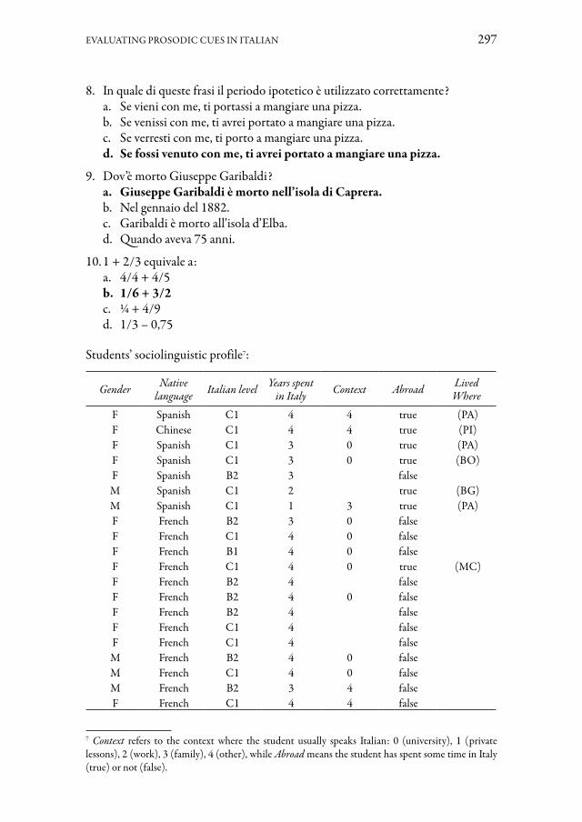
EVALUATING PROSODIC CUES IN ITALIAN 297
8. In quale di queste frasi il periodo ipotetico è utilizzato correttamente?a. Se vieni con me, ti portassi a mangiare una pizza.b. Se venissi con me, ti avrei portato a mangiare una pizza.c. Se verresti con me, ti porto a mangiare una pizza.d. Se fossi venuto con me, ti avrei portato a mangiare una pizza.
9. Dov’è morto Giuseppe Garibaldi?a. Giuseppe Garibaldi è morto nell’isola di Caprera.b. Nel gennaio del 1882.c. Garibaldi è morto all’isola d’Elba.d. Quando aveva 75 anni.
10. 1 + 2/3 equivale a:a. 4/4 + 4/5b. 1/6 + 3/2c. ¼ + 4/9d. 1/3 – 0,75
Students’ sociolinguistic profile7:
Gender Native language Italian level Years spent
in Italy Context Abroad LivedWhere
F Spanish C1 4 4 true (PA)F Chinese C1 4 4 true (PI)F Spanish C1 3 0 true (PA)F Spanish C1 3 0 true (BO)F Spanish B2 3 false M Spanish C1 2 true (BG)M Spanish C1 1 3 true (PA)F French B2 3 0 false F French C1 4 0 false F French B1 4 0 false F French C1 4 0 true (MC)F French B2 4 false F French B2 4 0 false F French B2 4 false F French C1 4 false F French C1 4 false M French B2 4 0 false M French C1 4 0 false M French B2 3 4 false F French C1 4 4 false
7 Context refers to the context where the student usually speaks Italian: 0 (university), 1 (private lessons), 2 (work), 3 (family), 4 (other), while Abroad means the student has spent some time in Italy (true) or not (false).

298 VALENTINA DE IACOVO, MARCO PALENA, ANTONIO ROMANO
Gender Native language Italian level Years spent
in Italy Context Abroad LivedWhere
F French C1 4 false F English C1 3 3 true (RM)M English C1 4 4 false F Spanish B2 4 false F French C1 3 0 true (TO)F Russian B1 3 0 true (RM)F Russian B2 2 true (RM)F French B1 3 4 true (RM)F French B2 4 0 true (RM)F English B1 3 true (TO)F Slovenian B2 2 4 false F Slovenian B1 2 true F Slovenian C1 4 0 false O Slovenian B1 3 false M English B1 4 3 false F Hungarian C1 4 4 false F English B1 2 0 false M Russian C1 3 true (VA)F English A1 2 0 false M English B2 2 4 false F Gaelic B1 2 false M English C1 3 0 true (BO)F Hungarian C1 4 4 true (TS)M Portuguese null 0 true (PI)F Spanish B2 1 0,2,3 true (AT)F Romanian null 2,0 true (TO)F null true (TO)M Armenian B2 3 true (TO)F Romanian C1 4 2,3,0,4 true (CN)F Portuguese C1 4 2,3,0 true (TO)M Romanian null 2,3,4,0,1 true (TO)F Serbian C1 4 0,4 true (TO)M Romanian C1 4 3,0,4 true (TO)M Portuguese B2 1 true (VC)F Spanish C1 4 2,3,0 true (TO)

DOI: 10.17469/O2108AISV000016
DUCCIO PICCARDI, FABIO ARDOLINO
Gaming variables in linguistic research. Italian scale validation and a Minecraft pilot study
This paper deals with the concept of gamified science and its recent applications to the linguistic field. We argue that, albeit promising, this paradigm still lacks analytical tools to model the effects of the peculiar experimental setting on the results obtained. After a theoretical introduction to the User Engagement and Gaming Literacy constructs, we present two validated Italian translations of scales representing them. Lastly, we test these two gaming variables in a pilot study on the postvocalic realizations of /k t/ in the Florentine variety. Results show that both variables positively condition the production of non-continuants (i.e., emphasized words) but through different underlying mechanisms.
Keywords: gamification, User Engagement, Gaming Literacy, Minecraft, Florentine gorgia
1. Gamification and scienceAn interactive museum panel, an app for competing with other fitness-enthusiasts, an online game to explore a tourist destination: these are only a few examples of gamified activities nowadays familiar also to those who are less used to videogames. As pointed out in the analysis by Deterding, Dixon, Khaled & Nacke (2011), the notion of gamification – enjoying growing success in the last two decades – defines the adoption of typical videogame elements (design patterns, interface mechanics, rewards) in non-game contexts. The ratio under the gamification of traditionally non-game activities lies in the ease with which gamified experiences trigger the user’s motivation, involvement, and entertainment, and, consequently, in the greater resolution with which the participants approach the completion of gamified tasks (Sailer, Hense, Mandl & Klevers, 2013).
In view of these opportunities, the development of gamified protocols in human sciences constitutes a natural outcome. Especially in data gathering, providing participants with entertaining tasks represents a crucial element to ensure the qualitative value of the collected data (Landers, Auer, Collmus & Armstrong, 2018). Gamified protocols have been applied in various research fields, generally bringing experimental advantages (Hamari, Koivisto & Sarsa, 2014).
As observed by Landers et al. (2018), however, the enthusiastic implementation of gamified approaches in many research scenarios has often underestimated the importance of critical reflection around the issues deriving from a naïve gamification of the investigation strategies (Rapp, Hopfgartner, Hamari, Linehan & Cena, 2019).

300 DUCCIO PICCARDI, FABIO ARDOLINO
On the basis of these assumptions, this work aims at exploring how two of the main variables linked to the participant’s performance in gamified protocols – namely, User Engagement (UE; § 2.1) and Gaming Literacy (GL; § 2.2) – interact with the collection of segmental data in a linguistic investigation focusing on a regional feature (the so-called gorgia, § 3.2) in the productions of Italian speakers from Florence. This experiment is described in § 3.4 and discussed in § 4. This work also provides a validation study of two Italian-translated tools for the quantification of UE and GL (§ 3.1). Before approaching the experimental discussion, the disciplinary field with which this study is collated (the gamification of linguistic research, § 1.1) will be addressed as well as the videogame used in the experiment: Minecraft (§ 1.2).
1.1 Gamified Linguistics
Linguistics has approached gamification relatively later in comparison to other humanistic fields. Nevertheless, the last decade has seen an increasing implementation of game elements in language studies and recently, the possibility of gathering linguistic data using gamified approaches has come to represent a trending topic explored in specialized publications and conferences (e.g., Hilton, Leemann, 2021). Applied Linguistics was one of the first fields to focus on the advantages of gamified approaches in improving language learning processes (Figueroa-Flores, 2015), followed by Cognitive Linguistics and Communication Studies. Already in the 2010s, the research by Yildirim, Narayanan & Potamianos (2011) constituted one of the first attempts to elicit conversational emotions in children using a gamified human-computer interaction. Thereafter, the study by Bos, Nissim (2015) comprised instead a first implementation of game-oriented tasks to facilitate the syntactic exploration of large digital corpora; the conclusion of the authors is that gamified approaches undoubtedly represent a noteworthy opportunity to simplify large-scale annotations.
The research developed by Leemann, Kolly, Purves, Britain & Glaser (2016) was one of the wider attempts to systematize the collection of speech data using gamified and participative methods. In Leemann, Schmid, Studer-Joho & Kolly (2018), a smartphone app was adopted to gather data regarding the regional variation of /r/ in Swiss dialects. The recent study by Duran, Lewandowski (2020) explicitly addressed the advantages of a videogame setting in an auditory discrimination task, specific measures having been adopted to quantify the subject’s familiarity with videogames. Participants completed both a classic and a gamified experiment. A regression model aimed at explaining reaction times highlighted an interaction between test type and levels of previous gaming experience. Surprisingly, compared to the results of non-gamers, the reaction times of experienced players proved to be longer in the gamified test. This pattern suggests their sensitivity to deviations from common gaming conventions.
The prosodic study by Buxó-Lugo, Toscano & Watson (2018; see also Toscano, Buxó-Lugo & Watson, 2015) represents one of the main methodological references for the investigations carried out in this work. Buxó-Lugo et al. (2018) specifically

GAMING VARIABLES IN LINGUISTIC RESEARCH 301
explored the predictor value exerted by participants’ engagement – underpinned by a gamified approach – on the discriminability of prosodic cues. Aiming at experimentally manipulating the participants’ engagement in communicative tasks, the authors adopted both a classic speech elicitation protocol (picture description) and a gamified one, consisting in the collaborative solution of simple puzzles in a Minecraft game environment. Higher levels of prosodic discriminability were observed in the gamified condition, and this was tentatively explained in relation to the greater spontaneity and emotional involvement triggered by gamification.
1.2 Minecraft: a playground for digital fieldwork
Minecraft (Persson, Bergensten, 2009) is a popular sandbox game periodically updated with new features. Similar to other sandbox games, Minecraft does not put the players in any predetermined ruleset, leaving them free to interact with the environment. The novelty introduced by this title is the block: in Minecraft, each scenario is composed of interactive cubic units. More than one hundred kinds of block can be found throughout the map, each one having distinct characteristics. At the cost of graphic realism, therefore, Minecraft allows a vast set of play possibilities.
The richness of the Minecraft experience has extended the fortune of this software far beyond the entertainment field. In 2016, a spin-off of the game was specifically developed for educational purposes (Minecraft: Education Edition; Mojang Studios, 2016; henceforth MEE). Compared to the original game, MEE introduces specific features to improve in-game teacher-student interaction. In line with its didactic goals, MEE is available free of charge for educational institutions and scholars, making this software an accessible tool for the design of gamified research protocols.
2. Two variables for gamified linguistic researchIn § 1.1, we encountered two pivotal phenomena for the interpretation of gamified linguistic data. Gamification leads to participant engagement which, in turn, is expected to engender spontaneous speech (Toscano et al., 2015); moreover, it taps into the participants’ knowledge of the digital medium, as gaming proficiency affects the responses to gamified inquiries (Duran, Lewandowski, 2020).
In Buxó-Lugo et al. (2018), engagement is conceptualized as a dichotomous label with a low (non-gamified task) and a high (gamified MEE task) level. However, no effort was made to detect engagement effects at the intra-task level: the exact linear relationships between discriminability of prosodic cues and participant engagement with the experiment remains therefore unexplored.
Duran, Lewandowski (2020) attempted to quantify individual proficiency by creating three pertinent variables: a binary isGamer (Yes/No) variable, the gaming frequency in days per week, and a score quantifying the number of game types played by the participants. Being presumably correlated, these three solutions struggle to
302 DUCCIO PICCARDI, FABIO ARDOLINO
manifest autonomous interpretability. Indeed, there is no explanation as to why only the gaming score is retained through the proposed model reduction procedure.
Overall, it seems that these implementations may still be open to operational refinements. In the following sections, we try to find solutions to the construction of meaningful speaker-dependent variables for gamified linguistic experiments. Therefore, with the aim of selecting tools for their quantification, a theoretical contextualization is provided concerning the related constructs of User Engagement and Gaming Literacy.
2.1 User Engagement
The creation of engaging technologies is a major field of interest in human-computer interaction. While discussions date back to the second half of the 1980s and the 1990s (e.g., Laurel, 1991), UE has stolen the spotlight since the advent of the participative web, pervasive technologies, and an increase in user choices (Attfield, Kazai, Lalmas & Piwowarski, 2011). O’Brien, Toms (2008: 941) provided a working definition of UE as a “category of user experience characterized by attributes of challenge, positive affect, endurability, aesthetic and sensory appeal, attention, feedback, variety/novelty, interactivity, and perceived user control”. In O’Brien (2016a), the author summarized her view on the major aspects of the construct, namely: a) UE is not one-dimensional, as it concerns affective, behavioral, and cognitive aspects; b) from the point of view of its temporality, UE manifests itself both during individual interactions and in subsequent states which condition the intention to re-engage; c) being bound to specific interactive events, UE takes contextuality seriously; and d) UE is not a dichotomous feature, its continuity being affected by user-, system-, and interaction-specific characteristics.
This summary highlights the shortcomings of treating UE as categorical and entirely task-dependent in gamified linguistic protocols (Buxó-Lugo et al., 2018). Variationist concerns add urgency to the need for a thorough investigation of the UE effects on linguistic data. Studies suggest that specific socio-demographic groups may react differently to engaging settings: Yang, Du, Wang & Wu (2019), observed a UE interaction with gender, while Di Gangi, Wasko (2016) observed one with age. Overall, these data suggest that the behavioral consequences of UE are not uniform across the population, so that adding interactions with social variables may unveil important data patterns.
Over the years, several UE quantification strategies have been devised. Among these, the UE Scale (UES) has received considerable attention, counting more than forty implementations in the most disparate contexts just a few years after its first release (O’Brien, 2016b). The UES was developed in O’Brien, Toms (2010) as a 31-item tool, divided into perceived usability, aesthetics, focused attention, felt involvement, novelty, and endurability. Eventually, two main issues related to the scale became evident (O’Brien, 2016b; O’Brien, Cairns & Hall, 2018): firstly, researchers perceived the UES as too cumbersome; secondly, reexaminations of the full scale suggested a rearrangement of its six factors to four (Wiebe, Lamb, Hardy

GAMING VARIABLES IN LINGUISTIC RESEARCH 303
& Sharek, 2014). O’Brien et al. (2018) addressed these two points by validating a new four-factor structure, the components of which were re-labeled as aesthetic appeal (AE), focused attention (FA), perceived usability (PU), and reward (RW). At the same time, the authors proposed a reduction to three items per factor, resulting in a 12-item short form.
To sum up, even though UE scales developed for the specific context of videogaming do exist (Abbasi, Ting & Hlavacs, 2017), the handiness of the UES short form and its many applications in heterogeneous research environments may favor its implementation in gamified linguistic research.
2.2 Gaming Literacy
In a broad sense, GL is part of the digital literacies and, more generally, the so-called new literacies. This label is a postmodernist attempt at challenging the monolithic and hierarchical acceptation of literacy as the mastery of reading and writing (Lankshear, Knobel, 2011). The internet plays a pivotal role in this decentralization process (Reinhardt, Warner & Lange, 2014: 161): thus, since their first definition (Gilster, 1997), digital literacies have been one of the most successful instantiations of this construct, being about “mastering ideas, not keystrokes” (Gilster, 1997: 15; Bawden, 2008: 18 and ff.). (Video)gaming literacy inherited the holistic nature of its hypernyms. This is a clear point in some of its most renowned definitions: for example, Gee (2003: 45-46) interlinked GL with a model of critical learning involving the decoding of a semiotic space and the transfer of knowledge to other domains and Zimmerman (2009) equated it to acquiring a set of cognitive, creative, and social skills in order to engage with the world and interpret its meanings. Nonetheless, mere system skills are still considered as core components of GL (Rosenberg, 2011: 20), and articulated models of literacy usually represent them in dedicated subcategories (e.g., Kringiel, 2012: 637).
Duran, Lewandowski (2020) focused on this aspect of literacy. Indeed, controlling the relative easiness of the participant-setup interaction is essential in any evaluation of research results (see, e.g., Rama, Black, Van Es & Warschauer, 2012). Mutatis mutandis, this point reflects classic concerns in sociolinguistics. Commenting on the manipulation of style attempted through the Labovian interview, Baugh (2001) observed that the stylistic variation triggered through reading sessions heavily depends on the participant’s literacy (in the traditional acceptation). If the hurdles experienced by the participant in interacting with the reading setup become too tough, the experiment ultimately fails. In addition to that, gaming-proficient participants can rely on their rooted habits and strategies, altering the intended effects of the manipulation. In another gamified perception experiment (a forced-choice categorization test), Lewandowski, Duran (2019) observed that the expected positive effect of mental flexibility, assessed through a Simon test, on correct categorizations was observable in the responses by female participants only. While gaming proficiency per se was not quantified, it was

304 DUCCIO PICCARDI, FABIO ARDOLINO
hypothesized that, being reputedly more gaming proficient, male participants may not rely on the benefits of higher mental flexibility.
Given the complex nature of GL, the development of scales going beyond the core component of skill is still far behind the refinement of UE. To the best of our knowledge, Rosenberg’s (2011) dissertation is the only systematic attempt at developing and validating a GL scale. This study led to an extensive 47-item, 5-factor scale, which is not suited to variable construction in non-GL-focused research (Rosenberg, 2011: 87). Interestingly enough, the first 22-item factor (Information and Systems Management), which included the core components of GL concerning mental and technical proficiency, drastically outperformed the others in terms of explained variance. Unfortunately, further revisions and reductions to the scale were never provided. This study also presented some adaptations to the gaming contexts of other reliable analytic tools. For example, devising a correlational counterpart to his GL scale for the sake of nomological validation, Rosenberg (2011) adopted the skill, challenge, and play scales designed in Novak, Hoffman (1997) to investigate the manifestation of flow in web users. Flow was conceptualized by Csikszentmihalyi (1975: 35 and ff.) as the achievement of the optimal experience in performing an activity. Rosenberg (2011: 27) argued that GL and flow share a conceptual linkage, namely that literate players are expected to reach high flow levels. In Rosenberg’s validation analysis, this assumption was generally met. In order to pinpoint a compact tool representing a construct that is at least closely tied to the core aspects of GL, we inspected the results concerning the main Information and Systems Management factor of Rosenberg’s original scale. This factor was most significantly correlated with and the best predictor of the five-item skill scale by Novak, Hoffman (1997). Thus, the strength of this theoretical relation may be considered reliable and it can be provisionally suggested that this manageable scale can be of some use in quantifying GL in gamified linguistic research1.
3. Gamified phonetics in Italian: scale validation and a Florentine pilot studyThis paragraph expounds the experimental component of this work. Firstly (§ 3.1), a validation study is presented of the Italian translations of the UES short form (O’Brien et al., 2018) and the skill scale adapted from Novak, Hoffman (1997) by Rosenberg (2011), interpreted here as a rough approximation to GL. Then, we test for the effectiveness of these scales by proposing an expansion to the Minecraft
1 An objection often raised concerning the formulation of items assessing GL is their genericity about videogame types. It is useful to report the argument of Klecka, Johnston, Bowman & Green (2021: 5) about conceptualizing GL through the total time spent videogaming. Klecka and colleagues observe that – in consideration of the vast articulation of today’s videogame market – cumulative time measurements can’t represent the knowledge of a subject on specific genres. While Novak, Hoffman’s (1997) skill scale does not face this problem, future GL research should aim to find a good compromise between genre representativity and handiness of the scales.

GAMING VARIABLES IN LINGUISTIC RESEARCH 305
linguistic agenda. While previous studies have focused on prosody (Buxó-Lugo et al., 2018), we try to export this method to the analysis of the segmental behavior of participants/gamers. Previous MEE studies hypothesized that engagement led participants to spontaneousness, which in turn makes them a) want to communicate effectively and b) produce emotion-driven utterances. Even though emotions were interpreted as not decisive, it should be noted that both phenomena converge on enhanced prosodic discriminability. From the segmental viewpoint, the effects of engagement may not be so straightforward for both phonetic and sociolinguistic reasons. While the facilitation of comprehension implies hyperarticulation (cf. Lindblom, 1990), spontaneity promotes enhanced variation (Barry, Andreeva, 2001), which also includes extreme reduction (e.g., Adda-Decker, Lamel, 2018). Labovian theorization of spontaneity (Labov, 2006: 64-65) promotes such complexification. In variationist terms, spontaneity is a condition that reduces the attention paid to speech and promotes more informal productions. This acceptation does not refer to the hyper/hypo continuum, as the “spontaneous” form is shaped by the indexical values attributed to specific variants2.
In § 3.2, we will introduce the object of our MEE experiment (§ 3.4), the Florentine gorgia (lit. ‘throat’; lenition of postvocalic plosives). This widespread phenomenon is characterized by reduced articulatory effort (Marotta, 2008), and the exceptions to its occurrence still need to be properly explained. The design of the gamified experiment will be described in a separate section (§ 3.3).
3.1 Italian UE and GL scales. Validation and internal structure
Since our study involves Italian participants, the experimental scales adopted to quantify UE (O’Brien et al., 2018) and GL (Rosenberg, 2011) were opportunely translated and re-validated. Preliminarily to the study, a three-step translation process was put in place to ensure the closeness of the Italian scales to the original ones. After the first translation into Italian, a bilingual computer engineer with experience in usability testing was asked to re-translate the items into English: items judged as not sufficiently similar to the original ones were reoperated; the process was repeated until agreement was met. The final items were randomized and arranged in a questionnaire, which was filled in by our participants using 5-point Likert scales (see the Appendix) after the completion of the MEE task (§ 3.3).
2 This cursory reference to speech spontaneity oversimplifies a major terminological and conceptual issue in linguistics and should be intended as merely expedient to underline the complexity of analyzing a communicative context in which engagement and spontaneity do not unequivocally point to a single direction in the hypo/hyper continuum. See Mereu, Vietti (2021) for a recent take on spontaneity. Also, in this section we do not make reference to any sociolinguistic acceptations of style other than Labovian attention paid to speech. Of course, other models of style, such as the audience design (i.e., style shifting is conditioned by the features of the audience) or speaker-centered approaches (i.e., style as agentive identity construction in a given context; Hernández-Campoy, 2016) might be of interest in the field of gamified phonetics. In fact, we have noted some traces of individual agency modulating our experimental results(§ 5, d).
306 DUCCIO PICCARDI, FABIO ARDOLINO
The trustworthiness of the Italian scales has been tested for reliability with widely adopted approaches. To improve the representativeness of the scales and obtain more accurate validation coefficients, the tests were carried out on the values returned by a pool of Italian participants (N = 32) which is larger than the Florentine subset analyzed in § 3.4 (N = 21). The results of the validation tests are summarized as follows.
The UES translated in this study consists of 12 items, grouped according to four distinct factors: aesthetic appeal (AE), focused attention (FA), perceived usability (PU), and reward (RW), each one comprising three items. A Cronbach’s alpha test was adopted to verify the internal reliability for each of the factors, returning acceptable values in three out of four cases: FA, α = .65; PU, α = .77; RW, α = .7. Concerning the AE factor, the returned alpha value (α = .58) almost reaches the lower acceptability threshold of 0.6: in view of the relatively small number of items, this value appears to be equally suitable for the study (Cortina, 1993). The global alpha returned by the scale (α = .8) is acceptable. Once the validity of the translated scale had been confirmed, a Confirmatory Factor Analysis (CFA) was carried out to verify the correspondence between the internal structures of the original and the translated scales (lavaan R package: R Core Team, 2020; Rosseel, 2012). The fit of the model based on the original UES four-factor structure returns the following indices: χ²(48) = 75.74, p = .007; Comparative Fit index (CFI) = .77; Tucker Lewis index (TLI) = .68; Root Mean Square Error of Approximation (RMSEA) = .134, p = .02. None of the computed fit indices achieve robust acceptability; however, due to the absence of abnormal values compared to the traditional thresholds and the potential effect induced on the coefficients by small samples (e.g., Chen, Curran, Bollen, Kirby & Paxton, 2008) we decided to accept the model for the aims of this study, deferring a more thorough inspection of the scale structure until the sample is sufficiently large.
The same validation analyses were carried out on the GL scale. Since no internal factor structure is envisaged for this tool (all the items refer to a one single factor), the test was modulated accordingly. The Cronbach alpha test carried out on the translated scale returns a robust index of α = .85, confirming the internal reliability of the Italian item battery. Following Novak, Hoffman (1997), a Principal Component Analysis was performed to explore the composition of the model: differently from the original skill scale, in which a single component exceeds the variance proportion minimum threshold of 10%, the translated scale returns two significant components, although with markedly unbalanced variance proportions (PC1 = 63%, PC2 = 16%). Since only the aggregate measure of the scale is under analysis in this study, a similar result does not seem to impact the trustworthiness of the obtained scale.
3.2 A gamified stress test for the gorgia. Brief history and working hypothesis
From the phonetic viewpoint, the gorgia is probably the most discussed linguistic feature of the Florentine (and Tuscan) way of speaking, counting an extensive

GAMING VARIABLES IN LINGUISTIC RESEARCH 307
academic tradition focused on its debated origins (Izzo, 1972). The gorgia is a series of consonant lenition phenomena in postvocalic position, including the variable weakening of the phonological voiceless plosives (/k t p/; e.g., [ˈseθa], seta, ‘silk’). The feature has a peculiar areal distribution stemming from the city of Florence, in which the phenomenon is most systematic; overall, the velar voiceless plosive is the preferred target, followed by /t/ and /p/, considering both parameters of frequency of occurrence and lenition degree (Giannelli, Savoia, 1979-1980).
Since the first acoustical analyses commented in Giannelli (1976) and Giannelli, Savoia (1978), researchers have struggled to provide categorical descriptions of the extreme variability of the gorgia phonetic outputs, which are not limited to fricatives (Marotta, 2001). By investigating a corpus of 938 potential gorgia realizations uttered by six young Florentine speakers, Sorianello (2001) realized that a) the most common Florentine gorgia realizations of /k t p/ are [ɦ θ ɸ] and b) non-continuant productions are overall rare (13.7%): among this small pool of occurrences, only 13 tokens (lenis and voiced plosives) pertain to /k t/. This pervasiveness of continuants differs from the distributions found in other Tuscan towns (Pisa, Siena), in which peculiar facets of non-continuity have been reported as “noticeably closed” fricatives (Giannelli, Savoia, 1978), preaspirated fricatives (Stevens, Hajek, 2005), semifricatives and homorganic affricates (Marotta, 2001). These variants consist of a more or less silent closure phase followed by a long release friction without a concentrated burst; from the perceptual viewpoint, they can be confused with plosives stricto sensu.
In order to gain a better understanding of the apparently rare Florentine non-continuants, previous research tried to pinpoint the circumstances of their occurrence. Giannelli (1976) and Giannelli, Savoia (1978: 43) reported very small percentages (3-5%) of Florentine non-continuants, used in fast and precise styles to stress specific words. Moreover, the authors referred to contextually motivated productions of Italian-like plosives, which may end up being hypercorrected through hyperarticulation (i.e., aspirated voiceless plosives). Other studies have stressed the roles of hyperarticulation and social factors in the selection of non-continuant variants in Florence. In another analysis of 500 potential gorgia contexts uttered by three Florentine speakers during a spontaneous dialogue, Sorianello (2003) did find a small percentage of stops. The author explains that “the occurrence of a voiceless stop is context-dependent: it occurs only in hyperarticulated or emphasized words” (Sorianello, 2003: 3082). Crucially, the data presented in Villafaña Dalcher (2008) goes way beyond this fragmentary evidence. Of her 660 gorgia contexts, 35% (more than double the number in Sorianello, 2001) was produced as non-continuants. These included stops (18%), fricated (or leaky) stops3 (13%) and semifricatives (4%) and were distributed among the three points of articulation (/k/: 14% of 231; /t/: 53% of 232; /p/: 39% of 197). While socio-indexical factors (such as the enactment
3 Fricated stops are here defined as produced with an incomplete closure (with visible noise) – burst – release temporal sequence. See Villafaña Dalcher (2006: 69) for a reference spectrogram (Florentine speech). In the corpus presented in Villafaña Dalcher (2008), they were mostly /t/ allophones.

308 DUCCIO PICCARDI, FABIO ARDOLINO
of supralocality) played a significant role in this pattern (Villafaña Dalcher, 2008: 310), the author also remarks that her experimental setup (read speech and the mention of Florentine Italian as the primary interest of the researcher) may have conditioned the emergence of standard-like productions.
To sum up, while the Florentine variety manifests pervasive weakening of postvocalic voiceless plosives, researchers also noted that there is room (albeit small) for non-continuity. However, to date, these variants have always been considered as collateral in the search for weakening. Turning back to the MEE gamified protocol, two elements of particular interest emerged in the review of gorgia studies: non-continuants a) are produced in order to stress specific words through hyperarticulation and b) are task-sensitive or, in other words, they can presumably be elicited through experimental manipulation. The MEE protocol is designed to trigger spontaneous speech, aiming at effective communication between players (§ 3). In the context of gorgia productions, UE may represent an ambiguous predictor of speaker behavior: on the one hand, the achievement of (sociolinguistic) spontaneousness may lead to a higher number of informal local variants (weakened gorgia tokens); on the other, engagement may motivate speakers to do well in the communicative MEE game through an enhancement of the phonetic cues of potential disambiguation (hyperarticulated non-continuant tokens). Conversely, the expected effects of core GL are more straightforward: as it is in the interest of expert gamers to communicate effectively in order to succeed they may make greater articulatory effort (i.e., through non-continuants). Therefore, in the following section, we will test the hypothesis that core GL positively affects the number of non-continuant variants of phonological voiceless plosives produced by Florentine speakers during a MEE session. UE is expected to follow this trend, but with less incisiveness. In fact, the predicted enhancement of discriminability (Buxó-Lugo et al., 2018) may be dampened by the presence of (sociolinguistically) spontaneous gorgia tokens. Moreover, by testing the interaction between GL and UE, we hypothesize that UE positively conditions the number of non-continuant productions, but only for those speakers manifesting a high GL. This follows the principle that a sufficient level of literacy is required in order to be sensitive to the intended experimental manipulation (cf. Baugh, 2001). In other words, from the viewpoint of an expert player who is more competent in “reading” the rules of the game, engagement could be less ambiguously related to the deployment of effective communication strategies (a sort of “literate engagement”).
3.3 A brief parenthesis on level design
The MEE level presented to participants consists of a small game arena shaped as a castle. At the start of the game, participants find themselves in front of the entrance and are free to familiarize themselves with the key controls. They receive all the game instructions from a non-playable character positioned near the main door. The goal of the level is to cross the castle from the first to the last of six consecutive communicating halls, which are connected by blocked doors, unlockable through

GAMING VARIABLES IN LINGUISTIC RESEARCH 309
the activation of levers in the correct sequence. Each hall is characterized by a similar set of elements, with some differences from one hall to another. The MEE developer toolset was inspected to retrieve all the objects corresponding to words whose Italian names include postvocalic /k t/. Due to the limitations of the game resources, a small set of 5 candidates was deployed to manipulate the environmental differences, while other elements were inserted as distractors. In detail, these elements are: a) an enclosure containing a sheep (It. pecora), the color of the wool varying from hall to hall; b) four frames representing vegetables (a potato, It. patata; a carrot, It. carota; a watermelon, It. cocomero), the kinds and order of which vary across the halls, with at least one of the three stimuli being repeated every time; c) a set of four mural tiles, encoding a distinct color sequence for each hall (distractors); d) four pots, containing flowers the colors of which vary across the halls (distractors); and e) a carpet (It. tappeto) with a distinct pattern depending on the hall.
The only way to discover the correct sequence of activation of the levers for each hall is to describe the exact content of the room to the researcher. Once all the information has been received, the experimenter identifies the room on a solution sheet and communicates the way out of the puzzle: at this point, the player can pull the levers to unlock the exit door. When the participant crosses the last castle door, another NPC notifies the end of the experience.
3.4 The gorgia at play
3.4.1 Participants and settingIn 2021, 21 Florentine speakers (11 females, 10 males; age M(SD) = 40.09(14.9)), took part in the MEE experiment. In most cases, participants (friends and acquaintances) were recruited by the first author. The sessions took place in three rooms in two Municipalities near Florence (Scandicci, Greve in Chianti).
3.4.2 MaterialsThis gamified experiment used the MEE level described in § 3.3.
3.4.3 ProcedureIn order to reduce potentially confounding factors of sociolinguistic nature, this stress test for the pervasiveness of the Florentine gorgia was performed by pairing our local informants with an in-group researcher (first author)4. Participants sat without headphones in front of a pc with the MEE level already running. The
4 Two issues – non-experimental in nature – strongly impacted the protocol designed for this study, namely a) the impossibility of using two MEE accounts at the same time and in the same game arena due to the restriction of the MEE free use plan and b) the impossibility, due to COVID-19 restrictions, of gathering together a greater number of participants within the same space, in order to perform the experimental task without the active intervention of the experimenter. Future redefinitions of the protocol should have as a primary goal the reduction of the researcher presence in the experimental task, through a) the generation of a totally in-game interaction between experimental actors and b) an elicitation method based on the interaction between two informants (a player and a helper, bearing the solution sheet), who are free to interact to solve the puzzles.

310 DUCCIO PICCARDI, FABIO ARDOLINO
researcher assisted the participants in navigating the very first part of the level, until they entered the castle. Then, the researcher stepped back diagonally and positioned himself at approximately two meters from the participant, facing the opposite direction while holding the solution sheet. While a complete fixation of the researcher’s behavior during the sessions was unfeasible, he scrupulously stuck to a small set of communicative rules: a) never intentionally solicit word repetitions; b) never steer the participant’s lexical choices toward the intended lexeme; c) avoid any unnecessary productions of the target words, while using paraphrases instead. All the tokens produced during a violation of these points were excluded from the analysis. The sessions were recorded through a Zoom H5 diagonally positioned in front of the participant (.wav 24 bit, 48 KHz). As the task instructions never mentioned language issues, participants were completely free to select any variant of their linguistic repertoire.
3.4.4 AnalysisThe acoustic analysis of the recorded sessions was performed in Praat (Boersma, Weenink, 2021). Target words were manually segmented, and their respective durations were extracted to compute a local speech rate measure (log(syllables/seconds)). Then, the postvocalic contexts of interest were inspected and coded as follows: 1, continuant (or deleted) segment (presence of a “canonical” Florentine gorgia); 0, non-continuant segment (absence of a “canonical” Florentine gorgia). The latter category included aspirated plosives (i.e., with voice onset time/VOT above 30 ms long; Cho, Ladefoged, 1999: 223), short-lag VOT plosives, leaky plosives (see § 3.2), and homorganic affricates. A series of statistical analyses were run to test our working hypotheses. A Generalized Linear Mixed-Effect model (lme4 R package: Bates, Maechler, Bolcher & Walker, 2015; the argument family was set to “binomial”) was built trying to predict the binary gorgia response from speaker’s UE (M(SD): 3.71(0.77)) and GL (M(SD): 2.97(1.38)) (main predictors); speaker’s sex, age, sophistication, and regionality, as well as consonant type (/k/ vs. /t/), stress position (stressed vs. post-stress syllable) and speech rate (controls). Sophistication was organized into three groups (adapted from Hudson, 1996), which were grounded on both occupation and education level: sophisticated (white-collar graduates, N = 6), rough (blue-collar non-graduates, N = 9), and mixed (intermediate scenarios, N = 6). A participant’s regionality (or degree of localness) was conceptualized through an adaptation of the Regionality Index (RI: Chambers, Heisler, 1999). Our RI consisted of four questions regarding the participant’s own birthplace and that of their parents, their place of residence, and relocations. The researcher coded the answers as follows: In the Province of Florence = 0; In another Tuscan Province = 1; In another Italian Region = 2; In another country = 3. We averaged these scores in order to obtain individual RI values (M(SD): 0.33(0.34)). Participant and word were added as random factors. Then, we investigated all the interactions between the main predictors and the control
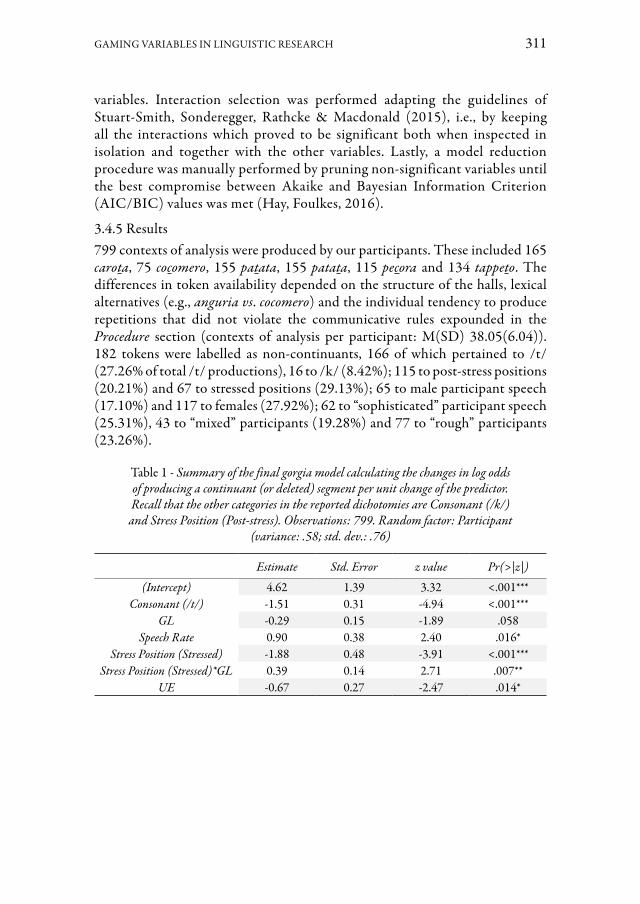
GAMING VARIABLES IN LINGUISTIC RESEARCH 311
variables. Interaction selection was performed adapting the guidelines of Stuart-Smith, Sonderegger, Rathcke & Macdonald (2015), i.e., by keeping all the interactions which proved to be significant both when inspected in isolation and together with the other variables. Lastly, a model reduction procedure was manually performed by pruning non-significant variables until the best compromise between Akaike and Bayesian Information Criterion (AIC/BIC) values was met (Hay, Foulkes, 2016).
3.4.5 Results799 contexts of analysis were produced by our participants. These included 165 carota, 75 cocomero, 155 patata, 155 patata, 115 pecora and 134 tappeto. The differences in token availability depended on the structure of the halls, lexical alternatives (e.g., anguria vs. cocomero) and the individual tendency to produce repetitions that did not violate the communicative rules expounded in the Procedure section (contexts of analysis per participant: M(SD) 38.05(6.04)). 182 tokens were labelled as non-continuants, 166 of which pertained to /t/ (27.26% of total /t/ productions), 16 to /k/ (8.42%); 115 to post-stress positions (20.21%) and 67 to stressed positions (29.13%); 65 to male participant speech (17.10%) and 117 to females (27.92%); 62 to “sophisticated” participant speech (25.31%), 43 to “mixed” participants (19.28%) and 77 to “rough” participants (23.26%).
Table 1 - Summary of the final gorgia model calculating the changes in log odds of producing a continuant (or deleted) segment per unit change of the predictor. Recall that the other categories in the reported dichotomies are Consonant (/k/)
and Stress Position (Post-stress). Observations: 799. Random factor: Participant (variance: .58; std. dev.: .76)
Estimate Std. Error z value Pr(>|z|)
(Intercept) 4.62 1.39 3.32 <.001***Consonant (/t/) -1.51 0.31 -4.94 <.001***
GL -0.29 0.15 -1.89 .058Speech Rate 0.90 0.38 2.40 .016*
Stress Position (Stressed) -1.88 0.48 -3.91 <.001***Stress Position (Stressed)*GL 0.39 0.14 2.71 .007**
UE -0.67 0.27 -2.47 .014*

312 DUCCIO PICCARDI, FABIO ARDOLINO
Figure 1 - Comparison of the interactions between GL and stress position (above), and GL, stress position and consonant (below). Evidently enough, the former is a generalization
of the /t/ distribution highlighted in the latter
The first full model had convergence issues, which we resolved by removing the “Word” factor with random intercept variance close to 05 and imposing a bobyqa optimizer with a high number of function evaluations. Our pipeline led us to a model with UE (negative effect), speech rate (positive effect), consonant (/t/ = negative effect), and an interaction between GL and stress position. The interaction between UE and GL was not significant (est. -.23; std. error: .2;
5 As an anonymous reviewer pointed out, given the very small pool of stimuli, a certain level of collinearity between “Word” and “Consonant” is not surprising.

GAMING VARIABLES IN LINGUISTIC RESEARCH 313
p = .26), even though it highlighted the expected pattern (i.e., UE conditions the production of non-continuants in the speech of participants with high GL, while low-GL participants are mostly unaffected). Since one of the few studies noting stress effects on the Florentine gorgia also investigated their interactions with plosive point of articulation (Sorianello, Bertinetto & Agonigi, 2005), we fitted a triple interaction between GL, plosive type, and stress position. This addition was significant (est. 1.14; std. error: .49; p = .019); however, while a slight improvement of AIC was noted (Δ>2), the triple interaction was unacceptable in terms of BIC (Δ>10). Fig. 1 compares the plot of the two interactions (sjPlot package: Lüdecke, 2021), highlighting that, while overall the participants with high levels of GL were unaffected by a positive effect of post-stress position on the gorgia continuant productions, this pattern ultimately pertains to the /t/ dataset only. Tab. 1 shows the final model.
4. DiscussionThe two validated Italian scales for UE and GL were put into action through a pilot gamified inquiry on the emergence of non-continuant allophones of /k t/ in postvocalic position in the Florentine variety. Exceptions to continuant gorgia productions may happen to emphasize specific words (Sorianello, 2003). For this reason, we inferred that a game based on the effectiveness of player communication might well be the ideal context for the observation of these variants. Moreover, we hypothesized that skilled (and, secondarily, more engaged) players enact a clearer and more effective communication with more non-continuants, and that having previous experience with videogames “unlocks” an additional effect of being engaged with the experimental setting on the production of non-continuity. While these assumptions were only partially met, UE and GL did influence the gorgia patterns, hinting at principles of regularity coherent with our theoretical expectations.
Our percentages of non-continuant allophones can be considered an intriguing compromise between the read speech of Villafaña Dalcher (2008) and the (semi- and) spontaneous conversations of Sorianello (2001, 2003). While /k/ is indeed pervasively produced as continuant, /t/ manifests a noticeable number of non-continuant alternatives. The Florentine gorgia prefers velar segments: this is one of the few, if not the only (Bertinetto, Sorianello & Ricci, 2007), distributional feature to be constantly retrieved in the relevant literature, and our statistical analysis makes no exception. However, this pattern does not explain why, across different studies, the percentages of non-continuity seem to vary the most in the realizations of /t/6. Apparently, being the middle ground in the front/back axis,
6 Recall that Sorianello (2003) noted about 3% of non-continuant /t/ (less than the non-continuant /k/ allophones), while Villafaña Dalcher (2008) presented a staggering 53% (far more than the non-continuant /p/ allophones!) and our study has a 27.26% of non-continuity.

314 DUCCIO PICCARDI, FABIO ARDOLINO
which conditions the degree of weakening in postvocalic position, /t/ is an optimal locus for the enactment of socially or communicatively driven variation. In fact, arguments have been advanced pointing at phonological and articulatory factors pressuring Tuscan /k/ towards lenition and /p/ towards (relative) preservation (i.e., consonant strength scales: Sorianello, 2001: 82; asymmetries in the Italian phonological system, which does not present back fricatives; combination of high intraoral pressure and reduction in tongue body constriction in V/k/V sequences: Marotta, 2008: 250-251, Villafaña Dalcher, 2006), so that /t/ realizations may be relatively more free to vary7.
Speech rate proved to be a significant predictor of the gorgia: at higher rates, the probability of observing a continuant production increases. This effect is coherent with the gradient decrease in segment duration, which was observed across the multiple degrees of weakening of the gorgia variants (Marotta, 2001; Sorianello, 20018), but is at odds with the relation between fast speech styles and non-continuity which was mentioned in Giannelli (1976) and Giannelli, Savoia (1978). We can tentatively argue that these two viewpoints can be reconciled by adopting a multidimensional acceptation of linguistic style (e.g., Moore, 2004) as an agentive practice of self-expression, which is de facto individual and linguistically complex, thus eluding the statistical patterns. In our corpus, there were indeed instances of “fast and precise” non-continuants; however, these occurrences were apparently very rare and speaker-specific, so that they did not constitute a problem for the robustness of the expected effect directionality.
Lastly, previous studies on the gorgia reported mixed results concerning stress position. With respect to Pisan data, Marotta (2001: 37-38) hypothesized that non-continuity is favored in stressed syllables. However, her analysis of variance failed to find support to this idea. In two computational studies based on Florentine data, Bertinetto et al. (2007) did not manage to find any stress effects on the gorgia, while Sorianello et al. (2005) observed a small trend confirming Marotta’s (2001) hypothesis, although non-continuity was favored in stressed syllables mostly in the case of dentals and bilabials. Our descriptive percentages seem to be in line with this phenomenon; however, keep in mind that our lexical pool was extremely limited because of MEE’s technical boundaries. In our set of stimuli, stressed syllables were represented as part of repeated CV sequences (i.e., patàta, cocòmero). As patterns of consonant lenition are sensitive to repetition avoidance (cf. Walter, 2007), any acritical generalization of this distribution should be avoided. Be that as it may, in our statistical model, the “Stress position” variable was ultimately part of a significant interaction with “GL”, which will be discussed next.
7 An alternative view on the issue highlights the cross-linguistic properties of the “coronals”, which justify their being the best target for variation in general (e.g., Barbera, Barth, Frassinelli & Lapesa, 2009: 114).8 See Cohen Priva, Gleason (2020) for clarifications on the causal relationships between speech rate, segment duration, and lenition.

GAMING VARIABLES IN LINGUISTIC RESEARCH 315
This short presentation of the linguistic variables conditioning the gorgia was expedient to comment on the effects of the two gaming scales. Most importantly, both GL and UE proved to be relevant predictors of participant behavior during the gamified experiment. This bodes well for their usefulness in unveiling linguistic patterns and promotes their adoption in other contexts of inquiry. With respect to GL, our initial hypothesis was drastically complexified through interaction testing. Rather than a general trend towards hyperarticulation, it seems that GL motivates specific communicative strategies involving the stress position variable. Fig. 1 shows that, while less skilled participants manifested a prosodic pattern favoring non-continuant productions in stressed syllables and continuant gorgia in post-stress position, the choices of more skilled gamers were stable across prosodic contexts. At first glance, this resembles Lewandowski, Duran’s (2019) failure to observe the expected effects of the experimental manipulation on the behavior of proficient subjects, who can presumably rely on alternative contextual resources. However, although statistically redundant, the triple interaction plot helps us to get a clearer picture of the specific behavioral difference between low- and high-GL participants. While both categories tend to have high percentages of continuant gorgia for postvocalic /k/, the predictions are more variegated for /t/. In the /t/ section of the plot, the major GL discrepancy lies in the production of tokens in post-stress position: high-GL speakers have a lower probability of producing a continuant gorgia in this context. Recall that post-stress /t/ was represented by tokens in word-final syllables (tappeto, carota, patata), while the /k/ counterpart was post-stress but word-internal (pecora). In Sorianello et al. (2005: 352), the authors conclude that weak gorgia allophones are most typical of phonological plosives in post-stress, prosodic-unit final syllables. A tentative explanation of the GL pattern could posit that the frequent struggles with the gaming interface caused hesitations in the speech of less proficient players, favoring prosodic-unit final productions and, consequently, word-final weakening. Conversely, the fluency of more skilled players did not hinder their overall communicative planning and eventual hyperarticulation. While an in-depth analysis of the prosodic structure of our sessions could clarify this issue, it should be stressed that, from the linguistic viewpoint, GL adapts to the generalities of the Florentine system and underlines local differences in the behavior of the participants.
The same cannot be stated for UE, which per se positively predicted a higher number of non-continuants in general. This result is quite surprising if we interpret the equation engagement : spontaneity in a sociolinguistic sense. A positive engagement in light-hearted, Florentine communication should have favored the local, informal gorgia continuant variants; conversely, the spontaneousness which is encapsulated by our UE seems to be related to the personal involvement in an effective communication. One way to break this impasse is to detach our variant selection process from the sociolinguistically meaningful continua of formality and localness (Villafaña Dalcher, 2008). While these axes are indeed pertinent to the gorgia variation, it should be kept in mind that the previous short descriptions
316 DUCCIO PICCARDI, FABIO ARDOLINO
of Florentine allophonic non-continuity do include pragmatic features (i.e., word emphasizing) which exist beyond them. In other words, a sociolinguistically spontaneous, casual Florentine conversation may well include postvocalic non-continuants: as long as they are used for stressing specific words, these allophones do not evoke any indexical incoherence. Therefore, we may argue that, with respect to the gorgia, UE is free to trigger phonetic spontaneousness, i.e., a removal of “cruise control” (Barry, Andreeva, 2001: 64) in the selection of hyper and hypo forms. Overall, our tentative interpretations suggest that, while GL describes how participants interact with the gamified setup in a technical sense, UE recounts their personal involvement, resulting in more general linguistic behaviors: in fact, its statistical significance is autonomous and not tied to another predictor.
Lastly, the lack of significance of the hypothesized interaction between GL and UE can be explained in relation to the extremely accessible mechanics of MEE. After a few initial struggles, even our 70-year-old participants who had never played a videogame in their entire lives successfully understood the rules and completed our levels. Therefore, GL did not appreciably filter the content of participant UE. In any case, as the related plot did point towards the expected trend, we might expect to find significant interactions in more complex gamified experiments.
5. Conclusions: current limitations and future directionsIn this study, we proposed a validation of the Italian short-form UES (O’Brien et al., 2018) and gaming skill scale (Rosenberg, 2011), which is here considered a rough approximation to GL. Although reliability tests are already acceptable, as our pool of participants is very limited, future replications of our results using larger Italian datasets may be called for. A larger number of responses would benefit also the internal structure analyses, the results of which are still far from optimal. At present, we tentatively recommend adopting these scales in their aggregate forms only and invite Italian researchers to experiment with their factor structures in other contexts.
The MEE experiment was succeful in proving the usefulness of the two gaming variables in linguistic research. GL and UE represent two different types of conditioning on linguistic production: the former seems to be mostly related to local adjustments to technical difficuties, while the latter was linked to general behavioral patterns because of the level of personal involvement in the task. We argue that the extreme accessibility of MEE somehow dampened the expected role of GL: future research should experiment with more complex communicative games such as Keep talking and nobody explodes (Steel Crate Games, 2015). Moreover, we are aware that our implementation of GL is rudimental and still in need of an effective summarization of its multifaceted nature (also concerning the diversity of contemporary videogame genres), and we stress that gamified research could vastly benefit from a dedicated scale construction process.

GAMING VARIABLES IN LINGUISTIC RESEARCH 317
The experiment has proved to be of dialectological interest as well, as it is the first to explicitly focus on the production of non-continuant variants of voiceless plosives in postvocalic position in the Florentine variety. The percentages of non-continuants, which were higher than in other spontaneous corpora (Sorianello, 2001, 2003), and the positive effect of UE on the preference for non-weakened allophones are small hints favoring the idea that these variants are produced for word emphasizing in specific discourse structures. However, this postulate should be refined in several ways: a) in order to reconcile the partially conflicting correlates of spontaneity and engagement (§§ 3, 3.2) with our UE results, we argued that non-continuity might well find its place in specific occurrences of spontaneous Florentine speech. Future research might be interested in quantifying spontaneity separately from engagement by counting the occurrences of specific indicators (e.g., laughs, disfluencies, etc.; Mereu, Vietti, 2021); b) the set of lexical targets was extremely limited and engendered ambiguity as the effect of multiple variables could not be effectively separated. While this was due to an intrinsic limitation of MEE, the research community should actively search for a workaround to this issue; c) a control, non-gamified experimental condition could help define the task-specific role of UE and GL by comparing the production of the same set of words in different circumstances (cf. Buxó-Lugo et al., 2018); d) while this pilot study has focused on a binary distinction between continuants and non-continuants, we suggest that drawing more precise coordinates of the emergence of the individual allophones could be an intriguing dialectological task. For example, to the best of our knowledge, this study was the first to experimentally replicate the Florentine postvocalic aspirated plosives observed in Giannelli, Savoia (1978). These allophones exclusively occurred in the speech of a retired teacher (see Fig. 2), who could have preferred extreme hyperarticulation in order to index precision (Drummond, Schleef, 2016). Are these allophonic selections idiosyncratic, or can we expect to find more systematic social patterns? How does indexicality merge with more general pragmatic roles of hyperarticulation? e) In-depth analyses of the prosodic and temporal aspects of the gamified sessions (hesitations, total completion time, etc.) could provide more complete pictures of the factors conditioning the produced speech from a segmental viewpoint.
Overall, gamified linguistic research is still at its title screen. Through the validation of gaming-specific variables, this field can enter new engaging levels of linguistic analysis.

318 DUCCIO PICCARDI, FABIO ARDOLINO
Figure 2 - Patata (‘potato’) uttered by a 71-years-old, female, white-collar participant with high UE (4.25) and very low GL (1). The first /t/ is produced as aspirated plosive
(VOT: 51 ms, covering the 41.8% of the total segment duration)
Bibliography
Abbasi, A.Z., Ting, D.H. & Hlavacs, H. (2017). Engagement in games: developing an instrument to measure consumer videogame engagement and its validation. In International Journal of Computer Games Technology, 10, 1-10. https://doi.org/10.1155/2017/7363925Adda-Decker, M., Lamel, L. (2018). Discovering speech reductions across speaking styles and languages. In Cangemi, F., Clayards, M., Niebuhr, O., Schuppler, B. & Zellers, M. (Eds.), Rethinking Reduction. Berlin/Boston: De Gruyter Mouton, 101-128. https://doi.org/10.1515/9783110524178-004Attfield, S., Kazai, G., Lalmas, M. & Piwowarski, B. (2011). Towards a science of user engagement (Position paper). In WSDM ‘11: Proceedings of the fourth ACM international conference on Web search and data mining, Hong Kong, China, 9-12 February 2011, 1-8.Barbera, M., Barth, M., Frassinelli, D. & Lapesa, G. (2009). Là dove il [ʃi] suona. Un’analisi parametrica delle sibilanti nell’Italiano di Carrara. In Romito, L., Galatà, V. & Lio, R. (Eds.), La fonetica sperimentale: metodo e applicazioni. Atti del IV Convegno Nazionale AISV. Torriana: EDK, 105-127.Barry, W., Andreeva, B. (2001). Cross-language similarities and differences in spontaneous speech patterns. In Journal of the International Phonetic Association, 31(1), 51-66. https://doi.org/10.1017/S0025100301001050Bates, D., Maechler, M., Bolker, B. & Walker, S. (2015). Fitting Linear Mixed-Effects Models Using lme4. In Journal of Statistical Software, 67(1), 1-48. https://doi.org/10.18637/jss.v067.i01Baugh, J. (2001). A dissection of style-shifting. In Eckert, P., Rickford, J.R. (Eds.), Style and sociolinguistic variation. Cambridge: Cambridge University Press, 109-118. https://doi.org/10.1017/CBO9780511613258.007Bawden, D. (2008). Origins and concepts of digital literacy. In Lankshear, C., Knobel, M. (Eds.), Digital Literacies: Concepts, Policies and Practices. New York: Peter Lang, 17-32.

GAMING VARIABLES IN LINGUISTIC RESEARCH 319
Bertinetto, P.M., Sorianello, P. & Ricci, I. (2007). Sulla gerarchia dei fattori che governano la gorgia. Un’applicazione dell’algoritmo di decisione C&RT. In Giordani, V., Bruseghini, V. & Cosi, P. (Eds.), Scienze Vocali e del linguaggio – Metodologie di valutazione e risorse linguistiche. Atti del III Convegno Nazionale AISV. Torriana: EDK, 167-180.Boersma, P., Weenink, D. (2021). Praat [Computer Program]. Phonetic Sciences, University of Amsterdam. Version 6.2, retrieved November, 15 2021 from https://www.fon.hum.uva.nl/praat/.Bos, J., Nissim, M. (2015). Uncovering noun-noun compound relations by gamification. In Megyesi, B. (Ed.), Proceedings of the 20th Nordic Conference of Computational Linguistics (NODALIDA 2015), Vilnius, Lithuania, 11-13 May 2015, 251-255.Buxó-Lugo, A., Toscano, J.C. & Watson, S.G. (2018). Effects of participants’ engagement on prosodic prominence. In Discourse Processes, 55(3), 305-323. https://doi.org/10.1080/0163853X.2016.1240742Chambers, J.K., Heisler, T. (1999). Dialect Topography of Quebéc City English. In Canadian Journal of Linguistics, 44(1), 23-48. https://doi.org/10.1017/S0008413100020703Chen, F., Curran, P.J., Bollen, K.A., Kirby, J. & Paxton, P. (2008). An Empirical Evaluation of the Use of Fixed Cutoff Points in RMSEA Test Statistic in Structural Equation Models. In Sociological Methods & Research, 36(4), 462-494. https://doi.org/10.1177/0049124108314720Cho, T., Ladefoged, P. (1999). Variation and Universals in VOT: Evidence from 18 Languages. In Journal of Phonetics, 27, 207-229. https://doi.org/10.1006/jpho.1999.0094Cohen Priva, U., Gleason, E. (2020). The causal structure of lenition: A case for the causal precedence of durational shortening. In Language, 96(2), 413-448. https://doi.org/10.1353/lan.2020.0025Cortina, J.M. (1993). What is coefficient alpha? An examination of theory and applications. In Journal of applied psychology, 78(1), 98-104. https://doi.org/10.1037/0021-9010.78.1.98Csikszentmihalyi, M. (1975). Beyond Boredom and Anxiety. The Experience of Play in Work and Games. San Francisco/London: Jossey-Bass.Deterding, S., Dixon, D., Khaled, R. & Nacke, L. (2011). From Game Design Elements to Gamefulness: Defining Gamification. In Proceedings of the 15th International Academic MindTrek: Envisioning future media environments, Tampere, Finland, 28-30 September 2011, 9-15.Duran, D., Lewandowski, N. (2020). Demonstration of a Serious Game for Spoken Language Experiments-GDX. In Lukin, S.M. (Ed.), Proceedings of the LREC 2020 Workshop Games and Natural Language Processing, Marseille, France, 11-16 May 2020, 68-78.Di Gangi, P.M., Wasko, M.M. (2016). Social Media Engagement Theory: Exploring the Influence of User Engagement on Social Media Usage. In Journal of Organizational and End User Computing, 28(2), 53-73. http://doi.org/10.4018/JOEUC.2016040104Drummond, R., Schleef, E. (2016). Identity in Variationist Sociolinguistics. In Preece, S. (Ed.), The Routledge Handbook of Language and Identity. London: Routledge, 50-65.

320 DUCCIO PICCARDI, FABIO ARDOLINO
Figueroa-Flores, J. (2015). Using Gamification to Enhance Second Language Learning. In Digital Education Review, 27, 32-54.Gee, J.P. (2003). What videogames have to teach us about learning and literacy. New York/Basingstoke: Palgrave Macmillan.Giannelli, L. (1976). Toscana. Pisa: Pacini.Giannelli, L., Savoia, L.M. (1978). L’indebolimento consonantico in Toscana. I. In Rivista Italiana di Dialettologia, II, 23-58.Giannelli, L., Savoia, L.M. (1979-1980). L’indebolimento consonantico in Toscana. II. Rivista Italiana di Dialettologia, III-IV, 38-101.Gilster, P. (1997). Digital Literacy. New York: John Wiley & Sons.Hamari, J., Koivisto, J. & Sarsa, H. (2014). Does Gamification Work? A Literature Review of Empirical Studies on Gamification. In Proceedings of the 47th Hawaii International Conference on System Sciences (HICSS ‘14), Waikoloa, HI, USA, 6-9 January 2014, 3025-3034.Hay, J., Foulkes, P. (2016). The evolution of medial /t/ over real and remembered time. In Language, 92(2), 298-330. https://doi.org/10.1353/lan.2016.0036Hernández-Campoy, J.M. (2016). Sociolinguistic styles. Chichester: Wiley-Blackwell.Hilton, N.H., Leemann, A. (2021). Editorial: using smartphones to collect linguistic data. In Linguistics Vanguard, 7(1), 1-7. https://doi.org/10.1515/lingvan-2020-0132Hudson, R.A. (1996). Sociolinguistics. 2nd edition. New York: Cambridge.Izzo, H.J. (1972). Tuscan & Etruscan. Toronto: University of Toronto Press.Kringiel, D. (2012). Learning to play: Video game literacy in the classroom. In Fromme, J., Unger, A. (Eds.), Computer games and new media cultures: A handbook of digital games studies. Berlin: Springer, 633-646. https://doi.org/10.1007/978-94-007-2777-9_40Klecka, H., Johnston, I., Bowman, N.D. & Green, C.S. (2021). Researchers’ commercial video game knowledge associated with differences in beliefs about the impact of gaming on human behavior. In Entertainment Computing, 38, 1-11. https://doi.org/10.1016/j.entcom.2021.100406Labov, W. (2006). The Social Stratification of English in New York City. 2nd Edition. Cambridge: Cambridge University Press. https://doi.org/10.1017/CBO9780511618208Landers, R.N., Auer, E.M., Collmus, A.B. & Armstrong, M.B. (2018). Gamification science, its history and future: definitions and a research agenda. In Simulation & Gaming, 49(3), 315-337. https://doi.org/10.1177/1046878118774385Lankshear, C., Knobel, M. (2011). New Literacies. Everyday Practices and Social Learning. 3rd Edition. Maidenhead/New York: Open University Press.Laurel, B. (1991). Computers as Theatre. Reading: Addison-Wesley.Leemann, A., Kolly, M.-J., Purves, R., Britain, D. & Glaser, E. (2016). Crowdsourcing Language Change with Smartphone Applications. In PLoS ONE, 11(1), 1-25. https://doi.org/10.1371/journal.pone.0143060Leemann, A., Schmid, S., Studer-Joho, D. & Kolly, M.-J. (2018). Regional Variation of /r/ in Swiss German Dialects. In Proceedings of Interspeech 2018, Hyderabad, India, 2-6 September 2018, 2738-2742.

GAMING VARIABLES IN LINGUISTIC RESEARCH 321
Lewandowski, N., Duran, D. (2019). Individual differences in implicit attention to phonetic detail in speech perception. In Proceedings of Interspeech 2019, Graz, Austria, 15-19 September 2019, 2255-2259.Lindblom, B. (1990). Explaining Phonetic Variation: A Sketch of the H&H Theory. In Hardcastle, W.J., Marchal, A. (Eds.), Speech Production and Speech Modelling. Dordrecht: Springer, 403-439. https://doi.org/10.1007/978-94-009-2037-8_16Lüdecke, D. (2021). sjPlot: Data Visualization for Statistics in Social Science. [R package] Version 2.8.8, retrieved June, 11 2021 from https://CRAN.R-project.org/package=sjPlot.Marotta, G. (2001). Non solo spiranti. La gorgia toscana nel parlato di Pisa. In L’Italia Dialettale, 62, 27-60.Marotta, G. (2008). Lenition in Tuscan Italian (Gorgia Toscana). In Brandão de Carvalho, J., Scheer, T. & Ségéral, Ph. (Eds.), Lenition and fortition. Berlin: Mouton de Gruyter, 235-271. https://doi.org/10.1515/9783110211443.2.235Mereu, D., Vietti, A. (2021). Dialogic ItAlian: the creation of a corpus of Italian spontaneous speech. In Speech Communication, 130, 1-14. https://doi.org/10.1016/j.specom.2021.03.002Mojang Studios (2016). Minecraft: Education Edition (PC Version) [Videogame]. Microsoft. Version 1.17.31, retrieved December, 15 2020 from https://education.minecraft.net/.Moore, E. (2004). Sociolinguistic Style: A Multidimensional Resource for Shared Identity Creation. In The Canadian Journal of Linguistics, 49(3/4), 375-396. https://doi.org/10.1017/S0008413100003558Novak, T.P., Hoffman, D.L. (1997). Measuring the flow experience among web users. Paper presented at the Interval Research Corporation.O’ Brien, H.L., Cairns, P. & Hall, M. (2018). A practical approach to measuring user engagement with the refined user engagement scale (UES) and new UES short form. In International Journal of Human-Computer Studies, 112, 28-39. https://doi.org/10.1016/j.ijhcs.2018.01.004O’Brien, H.L. (2016a). Theoretical perspectives on user engagement. In O’Brien, H.L., Cairns, P. (Eds.), Why Engagement Matters. Cham: Springer, 1-26. https://doi.org/10.1007/978-3-319-27446-1_1O’Brien, H.L. (2016b). Translating theory into methodological practice. In O’Brien, H.L., Cairns, P. (Eds.), Why Engagement Matters. Cham: Springer, 27-52. https://doi.org/10.1007/978-3-319-27446-1_2O’Brien, H.L., Toms, E.G. (2008). What is user engagement? A conceptual framework for defining user engagement with technology. In Journal of the American Society for Information Science and Technology, 59(6), 938-955. https://doi.org/10.1002/asi.20801O’Brien, H.L., Toms, E.G. (2010). The development and evaluation of a survey to measure user engagement. In Journal of the American Society for Information Science and Technology, 61(1), 50-69. https://doi.org/10.1002/asi.21229Persson, M., Bergensten, J. (2009). Minecraft (PC Version) [Videogame]. Mojang. Version 1.16, retrieved March, 03 2020 from https://www.minecraft.net/.

322 DUCCIO PICCARDI, FABIO ARDOLINO
R Core Team (2020). R: A language and environment for statistical computing. [Computer program] Version 4.0.5., retrieved March, 05 2021 from https://www.r-project.org/.Rama, P., Black, R., Van Es, E. & Warschauer, M. (2012). Affordances for second language learning in World of Warcraft. In ReCALL, 24(3), 322-338. https://doi.org/10.1017/S0958344012000171Rapp, A., Hopfgartner, F., Hamari, J. & Cena, F. (2019). Strengthening gamification studies: Current trends and future opportunities of gamification research. In International Journal of Human-Computer Studies, 127, 1-6. https://doi.org/10.1016/j.ijhcs.2018.11.007Reinhardt, J., Warner, Ch. & Lange, K. (2014). Digital games as practices and texts: New literacies and genres in an L2 German classroom. In Pettes Guikema, J., Williams, L. (Eds.), Digital Literacies in Foreign and Second Language Education. San Marcos: CALICO, 159-177.Rosenberg, K.A. (2011). Gaming Literacy: Construct Validation and Scale Construction. Master of Arts thesis, University of South Florida.Rosseel, Y. (2012). lavaan: An R Package for Structural Equation Modeling. In Journal of Statistical Software, 48(2), 1-36. https://doi.org/10.18637/jss.v048.i02Sailer, M., Hense, J., Mandl, H. & Klevers, M. (2013). Psychological perspectives on motivation through gamification. In Interaction Design and Architecture(s) Journal, 19, 28-37.Sorianello P., Bertinetto P.M. & M. Agonigi (2005). Alle sorgenti della variabilità della ‘gorgia’ fiorentina: un approccio analogico. In Cosi, P. (Ed.), La misura dei parametri. Aspetti tecnologici ed implicazioni nei modelli linguistici. Atti del I Convegno Nazionale AISV. Torriana: EDK, 327-362.Sorianello, P. (2001). Un’analisi acustica della ‘gorgia’ fiorentina. In L’Italia Dialettale, 62, 61-94.Sorianello, P. (2003). Spectral characteristics of voiceless fricative consonants in Florentine Italian. In Solé, M.J., Recasens, D. & Romero, J. (Eds.), Proceedings of the 15th International Congress of Phonetic Sciences, Barcelona, Spain, 3-9 August 2003, 3081-3084.Stevens, M., Hajek, J. (2005). Spirantization of/p t k/ in sienese Italian and so-called semi-fricatives. In Proceedings of Eurospeech/Interspeech 2005, Lisbon, Portugal, 4-8 September 2005, 2893-2896.Steel Crate Games (2015). Keep talking and nobody explodes (PC version). Steel Crate Games. Version 1.0, retrieved January, 18 2022 from https://keeptalkinggame.com/.Stuart-Smith, J., Sonderegger, M., Rathcke, T. & Macdonald, R. (2015). The Private Life of Stops: VOT in a Real-time Corpus of Spontaneous Glaswegian. In Laboratory Phonology, 6, 505-549. https://doi.org/10.1515/lp-2015-0015Toscano, J.C., Buxó-Lugo, A. & Watson, D.G. (2015). Using game-based approaches to increase level of engagement in research and education. In Dikkers, S. (Ed.), Teachercraft. Pittsburg: ETC Press, 139-151.Villafaña Dalcher, C. (2006). Consonant weakening in Florentine Italian: An acoustic study of gradient and variable sound change. Ph.D. Dissertation, Georgetown University.
GAMING VARIABLES IN LINGUISTIC RESEARCH 323
Villafaña Dalcher, C. (2008). Consonant weakening in Florentine Italian: a cross-disciplinary approach to gradient and variable sound change. In Language Variation and Change, 20(2), 275-316. https://doi.org/10.1017/S0954394508000021Walter, M.A. (2007). Repetition in Human Language. Ph.D. Dissertation, MIT.Wiebe, E.N., Lamb, A., Hardy, M. & Sharek, D. (2014). Measuring engagement in video game-based environments: investigation of the user engagement scale. In Computers in Human Behavior, 32, 123-132. https://doi.org/10.1016/j.chb.2013.12.001Yang, H., Du, H.S., Wang, L. & Wu, T. (2019). The influence of social support networks on health conditions via user engagement: gender as moderator. In Journal of Electronic Commerce Research, 20(1), 35-54.Yildirim, S., Narayanan, S. & Potamianos, A. (2011). Detecting emotional state of a child in a conversational computer game. In Computer Speech & Language, 25(1), 29-44. https://doi.org/10.1016/j.csl.2009.12.004Zimmerman, E. (2009). Gaming literacy: Game design as a model for literacy in the twenty-first century. In Perron, B., Wolf, M.J. (Eds.), The Video Game Theory Reader 2. New York: Routledge, 23-31.

324 DUCCIO PICCARDI, FABIO ARDOLINO
AppendixItalian UES Short form and Core GL(Skill) scale
The validated Italian translations of the UES Short form and the videogaming skill scale (O’Brien et al., 2018; Rosenberg, 2011) are presented here together with the original items in a non-randomized order. With respect to the UES, participants were asked to fill in the questionnaire while keeping in mind their experience with the Minecraft gaming session. Then, the skill items were introduced by an alert indicating their more general nature. The following semantic tags were assigned to the Likert values: 1 = ‘I totally disagree’; 2 = ‘I disagree’; 3 = ‘I neither disagree nor agree’; 4 = ‘I agree’; 5 = ‘I totally agree’.
FA 1. Mi sono immerso completamente in questa esperienza.[I lost myself in this experience.]FA 2. Il tempo è volato via mentre partecipavo al gioco.[The time I spent using Application X just slipped away.]FA 3. Sono stato preso da questa esperienza.[I was absorbed in this experience.]PU 1. (Reversed) Ho provato frustrazione a partecipare a questo gioco.[I felt frustrated while using this Application X.]PU 2. (Reversed) Ho trovato questo gioco disorientante.[I found this Application X confusing to use.]PU 3. (Reversed) Partecipare a questo gioco è stato faticoso.[Using this Application X was taxing.]AE 1. Questo gioco è stato accattivante.[This Application X was attractive.]AE 2. Questo gioco è stato esteticamente soddisfacente.[This Application X was aesthetically appealing.]AE 3. Questo gioco ha parlato ai miei sensi.[This Application X appealed to my senses.]RW 1. È valsa la pena di partecipare a questo gioco.[Using Application X was worthwhile.]RW 2. La mia esperienza è stata gratificante.[My experience was rewarding.]RW 3. Ho provato interesse per questa esperienza.[I felt interested in this experience.]
CoreGL(Skill) 1. Sono abile a giocare ai videogiochi.[I am skilled at playing video games.]CoreGL(Skill) 2. Mi considero esperto delle mosse, delle tecniche e delle strategie nei videogiochi a cui gioco.[I consider myself knowledgeable about moves, techniques, and strategies in/for the video games I play.]CoreGL(Skill) 3. (Reversed) Conosco meno i videogiochi rispetto alle altre persone.[I know less about games than most gamers.]CoreGL(Skill) 4. Giocare ai videogiochi mi risulta facile.[I find it easy to play video games.]CoreGL(Skill) 5. So come fare ciò che voglio quando gioco ai videogiochi.[I know how to do what I want when playing video games.]

DOI: 10.17469/O2108AISV000017
ELISA PELLEGRINO
Dynamics of short-term cross-dialectal accommodation. A study on Grison and Zurich German
This study investigates whether rhythmic features are object of accommodation between Grison and Zurich German (henceforth GRG and ZHG) speakers, insomuch as it was previously observed for vowel formants. Cross-dialectal rhythmic accommodation and its evoking/inhibiting factors (e.g., acoustic distance vs dialect markedness, new vs previously heard words) were examined in a corpus of pre- and post-dialogue recordings, performed by 18 pairs of GRG and ZHG speakers. Three rhythmic measures were designed which were based on cross-dialectal timing differences related to intervocalic sonorants gemination, open syllable lengthening and reduction of word-final vowels. Rhythmic accommodation was quantified measuring the acoustic distance in the realization of the three durational contrasts before and after dialogical interactions. Results revealed that, unlike vowel formants, rhythmic features did not evoke cross-dialectal adjustments under the given experimental circumstances.
Keywords: Phonetic Convergence, Speech Rhythm, Dialects in Contact, Speech Production.
1. IntroductionOur daily experience with vocal signals tells us that the way individuals sound like they do is extraordinarily variable. Individuals can unintentionally change their voice as a result of emotional states or fatigue, but can also adapt their vocal repertoire to respond to background conditions (e.g., noise vs quiet, Summers, Pisoni, Bernacki, Pedlow & Stokes, 1988; Traunmüller, Eriksson, 2000), interlocutors’ age and linguistic origin (e.g., Kemper, Finter-Urczyk, Ferrell, Harden & Billington, 1998; Kuhl, Andruski, Chistovich, Chistovich, Kozhevnikova, Ryskina, Stolyarova, Sundberg & Lacerda, Ferguson, 1997; Ferguson, 1975), or to convey personality traits (e.g, Hughes, Mogilski & Harrison, 2014; Carli, LaFleur & Loeber, 1995).
A phenomenon in speech communication which also affects the way we speak is vocal accommodation (Giles, 2008). This phenomenon is alternatively known as alignment (Pickering, Garrod, 2006), entrainment (Brennan, 1996), synchrony (Edlund, Heldner & Hirschberg, 2009), mimicry (Pentland, 2008) and chameleon effect (Chartrand, Bargh, 1999) and describes the tendency of interlocutors to adjust their verbal and non-verbal behaviour during interactions or after exposure to a communication partner or a model talker (e.g, Nguyen, Delvaux, 2015; Pardo, 2012; Ruch, Zürcher & Burkart, 2017 for review).
Two major theoretical frameworks have been proposed to explain accommodation. One is the Communication Accommodation Theory (CAT) (e.g., Giles, Mulac,

326 ELISA PELLEGRINO
Bradac & Johnson, 1987), which holds that speakers accommodate to their interlocutors, either by becoming more similar (convergence) or by accentuating individual differences (divergence). In this view, convergence and divergence signal speakers’ intention to express social closeness to or distance from their own interlocutors. In contrast to the social-oriented account of accommodation, there is the Interactive Alignment Model (IAM) proposed by Pickering & Garrod (2004). They argue that convergence is primed by an automatic, bidirectional link between speech perception and production that enhances mutual understanding between interlocutors. Evidence in support of both models exists. Recently, a hybrid approach has been proposed that sees accommodation as an unconscious phenomenon mediated by a range of social and linguistic constraints (e.g., Babel, 2012; Pardo, 2012; Pardo, Urmanche, Wilman & Wiener, 2017).
An example of accommodation which is linguistically and socially selective is the one observed between speakers of different dialects. Studies on cross-dialectal accommodation have, indeed, shown that more convergence is evoked when:– the distance between the phonetic repertoires of study participants is large (e.g.,
Babel, 2010, 2012; Walker, Campbell-Kibler, 2015; Ross, Lilley, Clopper, Pardo & Levi, 2021);
– cross-dialectal variants are perceptually salient (e.g, Mitterer, Muesseler, 2013; MacLeod, 2012; Troncoso-Ruiz, Elordieta, 2017), but less socially stereotyped (e.g., Babel, 2010; Walker, Campbell-Kibler, 2015; Clopper, Dossey, 2020);
– speakers have positive attitudes toward the residents of a dialectal region (Babel, 2010).
Acoustically, cross dialectal convergence has been typically measured in terms of vowel formants (e.g. Babel, 2010, Walker, Campbell-Kibler, 2015; Clopper, Dossey, 2020; Ross et al., 2021), word duration (Clopper, Dossey, 2020), word initial or final consonants/consonant clusters (e.g. MacLeod, 2012; Mitterer, Muesseler, 2013, Ross et al., 2021), and intonation patterns (e.g. D’Imperio, Cavone & Petrone, 2014; Troncoso-Ruiz, Elordieta, 2017; Romera, Elordieta, 2013). In terms of languages under scrutiny, most studies have been conducted in regional varieties of English (see a.o. Evans, Iverson, 2007; Babel, 2010; Clopper, Dossey, 2019, 2020), but research is also available for varieties of Spanish (e.g., MacLeod, 2012; Troncoso-Ruiz, Elordieta, 2017), French (e.g., Lelong, Bailly, 2010; Bullock, Gerfen, 2004) and Italian (D’Imperio et al., 2014).
Research on accommodation has been conducted also on Swiss German dialects (Werlen, Schlegel, 2006; Ruch, 2015, 2021; Pellegrino, Schwab & Dellwo, accepted), and the present study aims at advancing the knowledge of forms and factors affecting acoustic convergence between the dialectal varieties spoken in the Cantons of Zurich and Grisons.
1.1 Previous research on accommodation between Swiss German dialects
In a longitudinal study on 18 speakers from southern Switzerland relocated to Berne, Werlen & Schlegel (2006) showed that the amount of convergence towards

DYNAMICS OF SHORT-TERM CROSS-DIALECTAL ACCOMMODATION 327
the Bernese variety was largely accountable for by the speakers’ attitude towards their home or host region. Those who intended to go back or had fewer positive feelings towards the host region exhibited lower degrees of convergence. Ruch (2015) examined vowel convergence and divergence between pairs of GRG and ZHG speakers in pre- and post-dialogical items extracted from a picture naming task. She observed that ZHG speakers converged more to GRG speakers than vice versa, especially in low vowels and in words which served as stimuli in dialogical interactions. The same pattern, however, did not replicate when she investigated cross-dialectal accommodation including in the analysis items elicited through a different task (story retelling) (Ruch, 2021). The lack of convergence was interpreted in the light of the sociolinguistic status of Swiss German dialects which are mutually intelligible and share equal prestige. The author also used an agent-based modelling to simulate the change in vowel space in the absence of social and interactional factors. The results of the simulation showed that convergence was dependent on the variability of vowels. The dialect with the more dispersed distribution converged towards the dialect with the more compact distribution.
It has been shown, however, that patterns of convergence in one measure within a pair or within a speaker cannot be taken to be representative of pairs and speakers’ overall convergence patterns in other measures (Sanker, 2015; Cohen Priva, Sanker, 2018). Therefore, in this study we tested whether patterns of vowel convergence between GRG and ZHG speakers identified in Ruch (2015)1 would replicate for another set of acoustic features which varies between the two dialects, namely rhythmic properties. A preliminary investigation was conducted that compared the rhythmic distance between pairs of GRG and ZHG speakers before and after dialogical interactions (Pellegrino et al., accepted)2. The results of this study pointed to maintenance, in other words the rhythmic distance between pairs did not change substantially after participating to dialogical interactions, nor was it influenced by the degree of dialect markedness of the examined features. In view of the hypothesized influence of short-term accommodation on language variation and change (Trudgill, 1986), from this study only, however, it would have been premature to make any conclusion regarding the contribution of rhythmic patterns and the two dialects to the diffusion of linguistic innovation and dialectal levelling
1 The study on cross-dialectal rhythmic accommodation was designed, carried out and submitted to Studi AISV series before the paper by Ruch (2021) had been available online (10 September 2021). Therefore, the research questions and hypotheses of the present study are based on the findings reported in Ruch (2015).2 A detailed explanation as to the reasons why rhythmic features are supposed to be object of mutual adaptations is found in Pellegrino et al. (accepted). To put it simply, we based our assumption on evidence showing (1) rhythmic alignment in synchronous reading tasks (Cerda-Oñate, Toledo Vega & Ordin, 2021), and (2) rhythmic adjustments as function of interlocutors’ age and cognitive development (for comparisons between the rhythm of speech directed to infants and to adults, see Payne, Post, Astruc, Prieto & Vanrell, 2009; Leong, Kalashnikova, Burnham & Goswami, 2017). We took these findings as evidence that speakers may also adjust their rhythmic behavior after being exposed to a dialogue partner speaking a language with a distinct rhythmic pattern.

328 ELISA PELLEGRINO
in German speaking Switzerland. The analysis of accommodation performed in Pellegrino et al. (accepted), indeed, took the behaviour of the pair as whole. No distinction was made between items which were used during the diapix tasks and those which were not. Moreover, this type of analysis based on the pair is not particular informative in relation to the behaviour of individual ZHG and GRG speakers after being exposed to each other’s dialect. In the paper by Ruch (2015), indeed, accommodation within pair was documented but remarkable variability between speakers, speaker pairs and items was also observed. To gain an in-depth comprehension of dynamics of cross-dialectal rhythmic accommodation, in the present paper we compared pre- and post-dialogical productions within individual GRG and ZHG speakers in a pair (cf. §2.2) and distinguished between new items and those which served as the basis of the dialogical interactions.
Before turning to the specifics of the present study, however, we will first:1. sketch the sociolinguistic situation of German speaking Switzerland (cf. §1.2);2. present the cross-dialectal phonetic differences which legitimate the assumption
of inter-speaker rhythmic accommodation examined in the current research (cf. §1.3).
1.2 The sociolinguistic situation of German Speaking Switzerland
The sociolinguistic situation of German speaking Switzerland is characterized by medial diglossia. Standard German is used especially in writing, while Swiss German dialects are the default means of daily speech communication. The use of Swiss German dialects is not stigmatized in favour of standard variants. They are employed in public domains, in the media, in education (Scherrer, Samardžić & Glaser, 2019), as well as in inter-dialectal setting due to their highly mutual intelligibility.
Swiss German dialects share equal prestige (none of the dialect has the status of standard variety), whereas they rather vary in popularity, social attributes, and degree of perceived pleasantness (Ruch, 2018). For example, Bernese dialect is described as ‘colorful’, ‘cozy’, ‘countryside-ish’; Thurgau dialect as ‘bright’, ‘hard’, ‘unpopular’ or even ‘poisonous’. With respect to the two varieties examined in the present study, ZHG is perceived as ‘arrogant’, ‘unsympathetic’, ‘balanced,’ ‘common,’ ‘monotonous,’ and ‘dislikeable’, while GRG as ‘original,’ ‘warm,’ and ‘beautiful’ (for the attributes associated to dialects mentioned above, cf. studies in Leemann, Kolly & Nolan 2015, Ruch, 2018). It will be interesting to see whether these asymmetric attitudes towards GRG and ZHG will be reflected in the direction of cross-dialectal rhythmic accommodation.
1.3 Cross-dialectal differences between Zurich and Grison German
GRG and ZHG present noticeable phonetic differences (see a.o., Eckhardt, 1991; Fleischer, Schmid, 2006; Leemann, 2012). These have to do with:– the vowel system, principally in the quality of front vowels;– word-initial and post-vocalic k, realised in GRG as aspirated [kh], and in ZHG
either as velar fricative [x] or velar affricate [kx];

DYNAMICS OF SHORT-TERM CROSS-DIALECTAL ACCOMMODATION 329
– the speech rate that is lower in GRG than in ZHG;– intonation contours, with GRG showing high pitch-phrase initially and more
marked declination than ZHG.The two dialects also exhibit crucial segmental durational differences that lead to a different rhythmic organisation. These differences have mainly to do with:– intervocalic sonorants gemination in words ending in -e, (henceforth ISG);– open syllable lengthening (henceforth OSL);– vowel reduction in word final position (henceforth RedVow).Given that segmental timing properties are among the acoustic correlates of speech rhythm, in this paper we will refer to the three cross-dialectal differences in ISG, OSL and RedVow as rhythmic differences. In GRG intervocalic sonorants can be realized either as geminate or as singleton consonants, while in ZHG only as singletons (e.g., ‘Sun’: GRG > [‘sunnɐ]/[sunɐ]; ZHG > [‘sunǝ]). In GRG, open syllables can be either lengthened or not, while in ZHG the tendency to lengthen the open syllable has not been documented (e.g., ‘Sole’: GRG> [‘so:lɐ]/[‘solɐ]); ZHG > [‘solǝ]). In GRG, vowels in word-final position do not undergo vowel reduction in quality, and presumably either in duration, while in ZHG word-final vowels are always reduced (i.e., ‘Soup’ GRG> [‘suppɐ]; ZHG> [‘suppǝ]). That the differences in the quality of ending vowels also accompany distinct duration patterns is supported by findings in Leemann, Dellwo, Kolly & Schmid (2012). Here it was documented that the group of Midland dialects (to which ZHG belongs to) exhibited higher durational variability of vocalic intervals than the group of Alpine dialects (to which GRG belongs to). The lower durational variability of vocalic intervals of Alpine dialects was accounted for by the tendency of this dialectal group of retaining full vowels in unstressed position.
1.4 Research questions and hypotheses
In the present study, we examined whether:– speakers of GRG and ZHG converge in segmental timing properties in the same
direction as for vowel quality;– factors like acoustic distance/dialect markedness/word type (new or previously
heard items) account for patterns of accommodation within individual GRG and ZHG speakers.
If patterns of vowel convergence identified in Ruch (2015) replicate for segmental temporal properties, we expect that ZHG speakers converge more to their dialogue partners, while GRG speakers persist in their original behaviour (maintenance). Considering findings showing that speakers converge more for features that differ mostly between dialects (e.g., MacLeod, 2012; Ruch, 2015) and between the speakers and the model talkers (e.g., Babel, 2012), we hypothesise that more accommodation is evoked by RedVow than ISG and OSL. RedVow, indeed, is one of the features that best distinguishes the two dialects. GRG indeed exhibits open syllable lengthening – though in articulatory contexts other than ZHG – and presents longer nasal duration in -CCer words. Nevertheless, the realisation

330 ELISA PELLEGRINO
of reduced vowels is also a strong dialect marker for ZHG (Ruch, 2018). In view of evidence about less convergence for features that are dialect markers (e.g., Babel, 2010; Walker, Campbell-Kibler, 2015; Clopper, Dossey, 2020), we cannot exclude the possibility of speakers diverging or maintaining their original behaviour. Following the same line of reasoning (less convergence for dialect markers), between OSL and ISG the former should be less prone to accommodation since it is also perceived as another typical feature for GRG (Ruch, 2018). Based on findings showing more convergence for items previously heard than for new items (e.g., Goldinger, 1998; Nielsen, 2011; Ruch, 2015), we also expect more convergence in ZHG speakers for the items which were previously utilized in the diapix tasks.
2. MethodThe speech material and the method for calculating the scores of the three rhythmic measures are identical to the study by Pellegrino et al. (accepted). The operationalization of accommodation and the examination of factors affecting convergence, however, vary between the studies. In Pellegrino et al. (accepted), we quantified accommodation at the level of the pair, viz., we compared the Euclidean distance in the three ratio measures between members of a dyad in lexical items produced before and after two dialogical interactions. We also tested the effect of rhythmic measures (ISG, OSL and RedVow) on the amount of convergence. In the current study, instead, we quantify accommodation within individual GRG and ZHG members of a pair (henceforth accommodation within a speaker, cf. §2.2), and we test the interaction and the main effect of multiple factors evoking or inhibiting cross dialectal convergence (i.e., dialect, rhythmic measures, word type).
2.1 Speech Material
The corpus utilized in this study consisted of:– audio-recorded diapix tasks (i.e., problem-solving ‘spot the difference’ picture
tasks, cf. Van Engen, Baese-Berk, Baker, Choi, Kim & Bradlow, 2010) performed by 18 pairs of previously unacquainted GRG and ZHG female speakers.
– 18 pre- and 18 post-dialogue recordings (picture naming task and retelling a story based on a comic), performed individually by GRG and ZHG participants.
The diapix tasks were designed to elicit the target words present in picture naming task and story retelling. The present study reports on the data extracted from the picture naming task (henceforth PNT). As explained in Pellegrino et al. (accepted), the choice of selecting data from PNT was motivated by the fact that this permitted to control for the effect of the item variability in the assessment of: (a) cross-dialectal differences before the interaction; (b) differences in distance between ZHG and GRG speakers before and after the interaction. For the list of lexical items used in this study and the dialectal features they instantiate, cf. Tab. 1.

DYNAMICS OF SHORT-TERM CROSS-DIALECTAL ACCOMMODATION 331
Table 1 - List of items from PNT. Items in bold were utilized also in the diapix tasks (Adapted from Pellegrino et al., accepted)
ISG OSL RedVow
Brunnen, Pfanne, Sonne, Spinne, Welle
Besen, Esel, Graben, Käfer, Lupe, Nase, Schlafen, Melone
Besen, Brunnen, Flosse, Graben, Lampe, Lunge,
Lupe, Melone, Nase,Pfanne, Schlafen, Sonne,
Spinne, Suppe, Welle
2.2 Data Analysis and Statistics
To understand whether GRG and ZHG speakers produce the rhythmic features more similarly after participating in the diapix tasks, the following steps were taken:– From the pre- and post-dialogue recordings of individual speakers in PNT, we
extracted the lexical items instantiating the three target rhythmic features (ISG, OSL and RedVow).
– For every item, we automatically measured the duration of individual segments.We used the raw measures of segment duration to calculate the three ratio measures which were designed ad hoc to capture cross-dialectal differences in ISG, OSL and RedVow3.– For ISG, we calculated the ratio between the duration of intervocalic sonorants
(l, n) in -CCe words (e.g., Sonne, Welle) and that of the corresponding sonorant in -Ce words (l or n from the item Melone).
– For OSL, we calculated the ratio between the duration of stressed vowels in open syllables and that of the unstressed vowel within the same item.
– For RedVow, we calculated the ratio between the duration of stressed vowels in open and closed syllables and that of the unstressed vowel within the same item.
As shown in Pellegrino et al. (accepted), the speakers of the two dialects realised the three durational contrasts differently before the interaction, and this ensured that there was room for accommodation. GRG speakers scored significantly higher values as compared to ZHG speakers (Fig. 1). This was expected for ISG and OSL but not for RedVow. In GRG, indeed, intervocalic sonorants can be pronounced also as geminates, and open syllables can be lengthened, but the reduction of unstressed vowel is not that marked as in ZHG. This was, instead, imputed to the fact ZHG speakers might have not drastically reduced the duration of unstressed vowels in word-final position, as these vowels were subjected to pre-pausal lengthening.
3 We voluntarily refrained from using the so-called rhythmic metrics for the quantification of rhythmic accommodation since these have been typically applied to corpora of utterances with a sufficiently large amount of consonantal and vocalic intervals. The dataset used in this study, instead, consisted of individual bi-syllabic lexical items with two consonantal and vocalic intervals (except for Melone, which has three). These were deemed to be insufficient for an accurate analysis using rhythmic metrics.

332 ELISA PELLEGRINO
Figure 1 - Cross dialectal differences in ISG (left) and OSL (centre), RedVow (right) in pre-dialogue PNT (Pellegrino et al., accepted)
To quantify acoustical patterns of accommodation between GRG and ZHG speakers, we adapted methods typically utilized to quantify vowel convergence and divergence (Babel, 2012) to the rhythmic measures under study. Therefore, we measured the so-called accommodation within an individual (henceforth DD_speak) by calculating the following distance measures:– Distance 1 (d1): Euclidean distance in the score of a ratio measure between GRG
and ZHG speakers’ pre-dialogue production of a lexical item. If we take ‘Brunnen’ and ISG ratio as an example, d1 is calculated as follows: GRG pre [ISG – Brunnen] – ZHG pre [ISG – Brunnen].
– Distance 2 (d2): Euclidean distance in the score of a ratio measure between one speaker’s post-dialogue production and her dialogue partners’ pre-production of the same lexical item as in d1. So, if we consider the example above with ‘Brunnen’ and ISG, d2 is calculated as follows: GRG post [ISG – Brunnen] – ZHG pre [ISG – Brunnen], and ZHG post [ISG – Brunnen] – GRG pre [ISG – Brunnen].
After that, we calculated the difference in distance per individual speaker (DD_speak) and lexical item. For each member of a dyad this is computed by subtracting d2 from d1 (DD_speak = d2 – d1). Negative values of DD_speak show evidence of convergence, positive values indicate divergence, values centred around zero signal maintenance.
To test (a), i.e., whether one of the two dialects (ZHG) accommodates more and in which direction (convergence), we ran one Linear Mixed Effects Model with DD_speak as dependent variable and Dialect (GRG and ZHG) as fixed factor. The random part of the model comprised the intercept of Speakers and Lexical Items.

DYNAMICS OF SHORT-TERM CROSS-DIALECTAL ACCOMMODATION 333
To test (b), i.e., whether one of the two dialects accommodates more for the most acoustically distant ratio (RedVow), we tested the effect of the interaction between Dialect * Ratio Type (ISG, OSL, RedVow) on DD_speak, using a Linear Mixed Effects Model (Speakers and Lexical Items entered as random intercepts).
To test (c), i.e., whether previous exposure to target lexical items during the diapix tasks evokes more convergence than novel words in one of the two dialects, we tested the effect of a three-way interaction between Dialect * Ratio Type * Word Type (novel vs previously heard items) on DD_speaker, with a Linear Mixed Effects Model (Speakers and Lexical items entered as random intercepts). Statistical analyses were performed with R Studio (R Core Team 2020).
2.3 Results and Discussion
Regarding (a), i.e., whether ZHG speakers converged more towards GRG, the effect of Dialect on DD_speak was not significant [x2(1) =.0875, p = .767)]. As shown in Fig. 2, the values of DD_speak largely overlap between the two dialects and the peaks of both groups are centred around zero. Against the predictions, ZHG speakers did not modify the production of the segmental timing properties towards their interlocutors’ variety after dialogical interactions insomuch as they did for vowel qualities.
Figure 2 - Histogram showing the distribution of DD_speak values within speakers per dialect
This is even more evident if we observe the DD_speak scores of ZHG and GRG speakers across pairs per vowel formants (data from Ruch, 2015) and the segmental durational properties examined in this study (Fig. 3a-b). The scores for vowel formants were mostly negative for ZHG (Fig. 3a – top panel), meaning that they were more inclined to converge, despite a remarkable variability between speakers

334 ELISA PELLEGRINO
and pair (Ruch, 2015). For the segmental durational properties (Fig. 3b – bottom panel), instead, no clear pattern of convergence or divergence can be observed.
Figure 3a-b - Line chart showing the difference in distance within speaker (DD_speak) per dialect and pair for vowel formants (top panel, plot in Ruch, 2015),
and segmental durational properties (bottom panel). Dot represents average values, whisker error bar over all target words per speaker
With respect to (b), i.e., the hypothesis that ZHG and GRG are more prone to converge in RedVow as compared to OSL and ISG, the results of the statistical analysis have revealed that neither the interaction between Ratio Type and Dialect

DYNAMICS OF SHORT-TERM CROSS-DIALECTAL ACCOMMODATION 335
[x2(2)= .422, p = .971], nor the simple effects of Ratio Type and Dialect are significant [Ratio Type: x2(2)= 2.271, p = .678; Dialect: x2(1)= .087, p = .767].
Unlike other findings on cross-dialectal vowel accommodation showing more convergence for phonetically more distant vowels (e.g., Ruch, 2015; MacLeod, 2012), and more divergence for acoustic attributes perceived as strong dialect markers (e.g., Babel, 2010; Walker, Campbell-Kibler, 2015; Clopper, Dossey, 2020), none of the measures evoked a different degree of convergence in either dialect (Fig. 4). This was unexpected since the reduced/unreduced pronunciation of word final vowel (ɐ vs ǝ) is one of the features that best distinguishes the two dialects but is also a strong dialect marker. The same applies for OSL in comparison to ISG.
Figure 4 - Difference in distance within speaker (DD_speak) per ratio types and dialects
With respect to (c), i.e., more accommodation is evoked in items which were previously used in the diapix tasks, ZHG and GRG speakers contradict the predictions. In the study on vowel convergence (Ruch, 2015), GRG diverged and ZHG converged more for low vowels in items which served as the basis for the diapix tasks. A similar effect of new vs old words on convergence was found also in imitation studies by Goldinger (1998) and Nielsen (2011). In the case of rhythmic accommodation, instead, ZHG and GRG speakers’ inclination to rhythmically accommodate towards or away from their interlocutors’ variety was not promoted nor inhibited by previous exposure to the items utilized in the diapix tasks (Fig. 5).
The three-way interaction between Dialect * Ratio Type * Word Type was not significant [x2(7)= 2.263, p = .943)], nor were the two-way interactions between Word Type * Dialect [x2(1)= 3e-04, p = .986], Word Type * Ratio Type [x2(2) = 1.352,

336 ELISA PELLEGRINO
p = .508] and Ratio Type * Dialect [x2(2) = .0424, p = .979]. Insignificant were also the main effects of Dialect [x2(1) = .088, p = .766], Ratio Type [x2(2) = 2.536, p = .281] and Word Type [x2(1) = .701, p = .402].
Figure 5 - Difference in distance within speakers per ratio type, dialects and word type
The findings of this study coupled with those in Pellegrino et al. (accepted) point to rhythmic maintenance. Both when analysed at the level of the pair and at the level of individual speakers, unexpectedly, the rhythmic distance between and within members of a dyad did not significantly vary from pre- to post-dialogue productions. Accommodation was not influenced by socio-linguistic factors (e.g., acoustic distance, dialect markedness) or by previous exposure to the target lexical items (previously heard vs new items).
One possible explanation for the difference in accommodation between vowel formants (Ruch, 2015) and the rhythmic features examined here can be related to the perceptual salience of prosodic and spectral cues for dialect identification. This line of research suggests that listeners can make use of a variety of cues – both temporal and spectral – to identify a dialect. Although, the prominence of certain cues over others varies noticeably from study to study (see a.o. Boula de Mareüil, Vieru-Dimulescu, 2006; Vicenik, 2011; Fuchs, 2015; Ruch, 2018), when it comes to Swiss German dialects, however, the pronunciation of vowels has been shown to play a major role as compared to prosodic cues (Leemann, Siebenhaar, 2008; Leemann, Kolly & Nolan, 2016; Leemann, Kolly, Nolan & Li, 2018; for varieties of English, cf. Fuchs, 2015). Although some of the features under examination (RedVow and OSL) were deemed to be salient features of ZHG and GRG (Ruch, 2018), vowel

DYNAMICS OF SHORT-TERM CROSS-DIALECTAL ACCOMMODATION 337
pronunciation may have been more perceptually salient to interlocutors, and thus more susceptible to mutual adaptations between dialogue partners as the data in Ruch (2015) seem to suggest.
The results about rhythmic maintenance can also be explained along the same line of reasoning provided for the new data on cross-dialectal vowel accommodation (Ruch, 2021). The author imputed the conservative vowel production of ZHG and GRG speakers to the sociolinguistic situation of German Speaking Switzerland. As opposed to other countries, where dialects may be stigmatized in favour of standard variants, Swiss German dialects, instead, are employed in public and private domains, co-exist in everyday communicative situations due to their high mutual intelligibility, and share equal prestige (Scherrer et al. 2019). Although the two dialects vary in perceived likeability (Leemann et al. 2015; Ruch, 2018), in the absence of specific communication demands, ZHG and GRG speakers probably did not need to shift their pronunciation after being exposed to each other’s dialect. Given that the speech produced during the diapix tasks was not object of the present investigation, we cannot, however, exclude that rhythmic adjustments between dialogue partners happened in the course of interactions but were not retained in post-dialogue productions.
There might be, however, explanations of different nature for the lack of a clear effect of speakers’ dialect and word type on rhythmic accommodation. One for example may have to do with the small number of speakers (18 per dialect) and items (5 for ISG, 8 for OSL and 15 for RedVow). It is also plausible that by chance the pairing of GRG and ZHG speakers (at the corpus collection stage) resulted in 18 pairs with varying degree of baseline distance between the dialogue partners. This has been shown to be problematic for measurements of convergence based on the difference in distance approach (DD speak) used in research on phonetic convergence (Cohen Priva, Sanker, 2019). If the baseline distance is small, there is not much room for convergence, while the possibility of obtaining divergence is high. On the contrary, with large baseline distance, convergence can be overestimated. With a larger dataset, including data from the other tasks of the corpus, it would be interesting to see whether the same patterns of accommodation would replicate using the statistical model proposed by Cohen Priva, Sanker (2019). This overcomes the ‘baseline bias’ of the difference in distance approach, by taking the subject’s and interlocutor’s baselines as predictors of each subject’s performance in mixed-effects linear regression.
Another factor which would deserve further investigation is the degree of within speakers’ variability in the production of the examined rhythmic patterns prior to dialogical interactions. The results of a recent investigation examining computer simulations and experimental data from real interactions have, indeed, shown that the intrinsically more variable speaker of a dyad is the one who converges to the partner when accommodation takes place (Lee, Goldstein, Parrell & Byrd, 2021). Similarly, the results of the agent-based modeling of dialect contact reported in Ruch (2021) revealed that the dialect with the more dispersed distribution

338 ELISA PELLEGRINO
converged towards the dialect with the more compact distribution. It would be thus interesting to test whether the speakers who maintain their rhythmic properties in post-dialogue productions are those with reduced acoustic variability in pre-dialogue recordings.
3. ConclusionsThe results on rhythmic accommodation, together with findings on vowel convergence, based on the same corpus of lexical items in pre- and post-dialogue picture naming tasks, confirm the great complexity of the phenomenon of vocal accommodation. In line with findings showing that patterns of acoustic convergence are extremely variable within pairs or within speakers (Sanker, 2015; Cohen-Priva, Sanker, 2018), in this study the results on vowel convergence (Ruch, 2015) did not replicate for rhythmic accommodation. If ZHG speakers tended to converge more towards their dialect partner in terms of vowel formants, GRG and ZHG speakers tended to maintain their original rhythmic realization after being exposed to one another’s dialect. Interpretations of accommodation based on phonetic distance and word type which were shown to apply for vowel formants do not, instead, hold for rhythmic patterns. Framing the results in the light of hypothesized effect of short-term accommodation on language variation and change (Trudgill, 1986), we can tentatively assume that vowel quality characteristics may play a major role in the diffusion of linguistic innovations and dialectal levelling in German speaking Switzerland. Under the given experimental conditions, segmental timing features, indeed, were less prone to accommodation as opposed to vowel formants. In view of the more recent data on vowel maintenance (Ruch, 2021), these assumptions will warrant further research based on the more spontaneous tasks of the corpus, or using data collected in more ecologically valid communicative situations. Our data are based on isolated lexical items from a picture naming task without any pragmatic context, and this is certainly a type of speech that typically does not play a large role in everyday communication.
AcknowledgmentsThis research was supported by the University Research Priority Program (URPP) “Language and Space” of the University of Zurich (UZH). The author would like to thank Hanna Ruch for the corpus, Sandra Schwab for the feedback on the statistical procedure, and the reviewers for their helpful comments on an earlier version of this manuscript.

DYNAMICS OF SHORT-TERM CROSS-DIALECTAL ACCOMMODATION 339
Bibliography
Babel, M. (2010). Dialect divergence and convergence in New Zealand English. In Language in Society, 39(4), 437-456. https://doi:10.1017/S0047404510000400.Babel, M. (2012). Evidence for phonetic and social selectivity in spontaneous phonetic imitation. In Journal of Phonetics, 40, 117-189. https://doi.org/10.1016/j.wocn.2011.09.001.Boula de Mareüil, P., Vieru-Dimulescu, B. (2006). The contribution of prosody to the perception of foreign accent. Phonetica, 63(4), 247-267. 10.1159/000097308.Brennan, S.E. (1996). Lexical entrainment in spontaneous dialog. Proceedings of the International Symposium on Spoken Dialogue, Philadelphia, PA, 41-44.Bullock, B., Gerfen, C. (2004). Phonological convergence in a contracting language variety. In Bilingualism: Language and Cognition, 7(2), 95-104. 10.1017/S1366728904001452.Carli, L.L., LaFleur, S.J. & Loeber, C.C. (1995). Nonverbal behavior, gender, and influence. In Journal of Personality and Social Psychology, 68(6), 1030-1041. https://doi.org/10.1037/0022-3514.68.6.1030.Cerda-Oñate, K., Toledo Vega, G. & Ordin, M. (2021). Speech rhythm convergence in a dyadic reading task. In Speech Communication, 131, 1-12. https://doi.org/10.1016/j.specom.2021.04.003.Chartrand, T.L., Bargh, J.A. (1999). The chameleon effect: the perception-behavior link and social interaction. In Journal of Personality and Social Psychology, 76 (6), 893-910. https://doi.org/10.1037/0022-3514.76.6.893.Clopper, C.G., Dossey, E. (2019). Phonetic convergence and divergence in the American Midwest. In The Journal of the Acoustical Society of America, 145(3), 1930-1931.Clopper, C.G., Dossey, E. (2020). Phonetic convergence to Southern American English: Acoustics and Perception. In The Journal of the Acoustical Society of America, 147(1), 671-683. https://doi.org/10.1121/10.0000555.Cohen Priva, U., Sanker, C. (2018). Distinct behaviors in convergence across measures. Annual Conference of the Cognitive Science Society, Madison, WI, 1518-1523.Cohen Priva, U., Sanker, C., (2019) Limitations of difference-in-difference for measuring convergence. Laboratory Phonology 10(1), 15, 1-29. https://doi.org/10.5334/labphon.200.D’Imperio, M., Cavone, R. & Petrone, C. (2014). Phonetic and phonological imitation of intonation in two varieties of Italian. In Frontiers in Psychology, 5:1226. https://doi.org/10.3389/fpsyg.2014.01226.Eckhardt, O. (1991). Die Mundart der Stadt Chur. Zürich: Phonogrammarchiv der Universität Zürich.Edlund, J., Heldner, M. & Hirschberg, J. (2009). Pause and gap length in face-to-face interaction. 10th Annual Conference of the International Speech Communication Association, 2779-2782.Evans, B.G., Iverson, P. (2007). Plasticity in vowel perception and production: a study of accent change in young adults. In Journal of the Acoustical Society of America, 121, 3814-3826. 10.1121/1.2722209.
340 ELISA PELLEGRINO
Ferguson, C.A. (1975). Toward a characterization of English foreigner talk. In Anthropological Linguistics, 17(1), 1-14. https://doi.org/10.2307/30027270.Fleischer, J., Schmid, S. (2006). Zurich German. In Journal of the International Phonetic Association, 36, 243–253. 10.1017/S0025100306002441.Fuchs, R. (2015). You’re not from around here, are you? In Delais-Roussarie, E., Avanzi, M. & Herment, S. (Eds.) Prosody and Language in Contact. Berlin: Springer, 123-148.Giles, H. (2008). Communication accommodation theory. In Baxter, L.A., Braithwaite, D.O. (Eds.). Engaging theories in interpersonal communication: Multiple perspectives. Thousand Oaks: Sage Publications, 161-173.Giles, H., Mulac, A., Bradac, J.J. & Johnson, P. (1987). Speech Accommodation Theory: The first decade and beyond. In Annals of the International Communication Association, 10(1), 13-48. https://doi.org/10.1080/23808985.1987.11678638.Goldinger, S.D. (1998). Echoes of echoes? An episodic theory of lexical access. Psychological Review, 105(2), 251-279. 10.1037/0033-295x.105.2.251.Hughes, S.M., Mogilski, J.K. & Harrison, M.A. (2014). The perception and parameters of intentional voice manipulation. In Journal of Nonverbal Behavior, 38(1), 107-127. https://doi.org/10.1007/s10919-013-0163-z.Kemper, S., Finter-Urczyk, A., Ferrell, P., Harden, T. & Billington, C. (1998). Using elderspeak with older adults. In Discourse Processes, 25(1), 55-73. https://doi.org/10.1080/01638539809545020.Kuhl, P.K., Andruski, J.E., Chistovich, I.A., Chistovich, L.A., Kozhevnikova, E.V., Ryskina, V.L., Stolyarova, E.I., Sundberg, U. & Lacerda, F. (1997). Cross-Language analysis of phonetic units in language addressed to infants. In Science, 684-686. 10.1126/science.277.5326.684.Lee, Y., Goldstein, L., Parrell, B. & Byrd, D. (2021). Who converges? Variation reveals individual speaker adaptability. In Speech Communication, 131, 23-34. https://doi.org/10.1016/j.specom.2021.05.001.Leemann, A. (2012). Swiss German Intonation Patterns. Amsterdam: John Benjamins Publishing Company.Leemann, A., Dellwo, V., Kolly, M.-J. & Schmid, S. (2012). Rhythmic variability in Swiss German dialects. Proceedings of the 6th International Conference on Speech Prosody, Shanghai, China, 22-25 May 2012, 607-610.Leemann, A., Kolly, M.-J., & Nolan, F. (2015). It’s not phonetic aesthetics that drives dialect preference: The case of Swiss German. Proceedings of the 18th International Congress of Phonetic Sciences, Glasgow, UK, 10-14 August 2015.Leemann, A., Kolly, M.-J. & Nolan, F. (2016). Identifying a speaker’s regional origin: The role of temporal information. Proceedings of Speech Prosody, Boston, MA, 31 May-3 June 2016.Leemann, A., Kolly, M.-J., Nolan, F. & Li, Y. (2018). The role of segments and prosody in the identification of a speaker’s dialect. In Journal of Phonetics, 68, 69-84. https://doi.org/10.1016/j.wocn.2018.02.001.

DYNAMICS OF SHORT-TERM CROSS-DIALECTAL ACCOMMODATION 341
Leemann, A., Siebenhaar, B. (2008). Perception of dialectal prosody. Proceedings of the 9th Annual Conference of the International Speech Communication Association, Brisbane, Australia, 22-26 September 2008, 524-527.Lelong, A., Bailly, G. (2010). Study of the phenomenon of phonetic convergence thanks to speech dominoes. Proceedings of Analysis of Verbal and Nonverbal Communication and Enactment. The Processing Issues – COST 2102 International Conference, Budapest, Hungary, September 7-10, 273-286.Leong V., Kalashnikova, M., Burnham, D. & Goswami, U. (2017). The temporal modulation structure of infant-directed speech. In Open Mind: Discoveries in Cognitive Science, 1, 78-90. https://doi.org/10.1162/OPMI_a_00008.MacLeod, B. (2012). The effect of perceptual salience on phonetic accommodation in cross-dialectal conversation in Spanish. PhD Thesis, University of Toronto.Mitterer, H., Müsseler, J. (2013). Regional accent variation in the shadowing task: Evidence for a loose perception-action coupling in speech. In Attention, Perception & Psychophysics, 75, 557-575. https://doi.org/10.3758/s13414-012-0407-8.Nielsen, K. (2011). Specificity and abstractness of VOT imitation. In Journal of Phonetics, 39(2), 132-142. https://doi.org/10.1016/j.wocn.2010.12.007.Nguyen, N., Delvaux, V. (2015). Role of imitation in the emergence of phonological systems. In Journal of Phonetics, 53, 46-54. https://doi.org/10.1016/j.wocn.2015.08.004.Pardo, J. (2012). Reflections on phonetic convergence: Speech perception does not mirror speech production. In Language and Linguistics Compass, 753-767. https://doi.org/10.1002/lnc3.367.Pardo, J.S., Urmanche, A., Wilman, S., & Wiener, J. (2017). Phonetic convergence across multiple measures and model talkers. In Attention, Perception, & Psychophysics, 79(2), 637-659. https://doi.org/10.3758/s13414-016-1226-0.Payne, E., Post, B., Astruc, L., Prieto, P. & Vanrell, M. d. M. (2009). Rhythmic modification in child directed speech. In Working Papers in Linguistics, Philology & Phonetics, 12, 123-144. http://www.ling-phil.ox.ac.uk/files/uploads/OWP2009.pdf.Pellegrino, E., Schwab S. & Dellwo, V. (accepted). Do speakers converge rhythmically? A study on Grison and Zurich German, Loquens.Pentland, A. (2008). Honest Signal: How they shape our world. Cambridge: MIT Press.Pickering, M.J., Garrod, S. (2004). Toward a mechanistic psychology of dialogue. In Behavioral & Brain Sciences 27, 169-190. 10.1017/S0140525X04000056.Pickering, M.J., Garrod, S. (2006). Alignment as the basis for successful communication. In Research on Language and Computation 4 (2–3), 203-228. 10.1007/s11168-006-9004-0.R Core Team. (2020). A language and environment for statistical computing. [Computer Program] Version 4.0.1, retrieved 6 June 2020 from https://www.r-project.org/.Romera, M., Elordieta, G. (2013). Prosodic accommodation in language contact: Spanish intonation in Majorca. In International Journal of the Sociology of Language, vol. 2013, no. 221, 127-151. https://doi.org/10.1515/ijsl-2013-0026.Ross, J., Lilley, K., Clopper C., Pardo J. & Levi, S. (2021). Effects of dialect-specific features and familiarity on cross-dialect phonetic convergence. In Journal of Phonetics, 86, 101041, 1-23. https://doi.org/10.1016/j.wocn.2021.101041.

342 ELISA PELLEGRINO
Ruch, H. (2015). Vowel convergence and divergence between two Swiss German dialects. Proceedings of the 18th International Congress of Phonetic Sciences, Glasgow, UK, 10-14 August 2015.Ruch, H. (2018). The role of acoustic distance and sociolinguistic knowledge in dialect identification. In Frontiers in Psychology, 9:818. https://doi.org/10.3389/fpsyg.2018.00818.Ruch, H. (2021). Dialect contact in real interaction and in an agent-based model. In Speech Communication, 134, 55-70. https://doi.org/10.1016/j.specom.2021.09.003.Ruch, H., Zürcher, Y. & Burkart, J.M. (2017). The function and mechanism of vocal accommodation in humans and other primates. In Biol Rev Camb Philos Soc. 2018 May, 93(2), 996-1013. 10.1111/brv.12382.Sanker, C. (2015). Comparison of phonetic convergence in multiple measures. In Cornell Working Papers in Phonetics and Phonology 2015, 60-75.Scherrer, Y., Samardžić, T. & Glaser, E. (2019). Digitising Swiss German: How to process and study a polycentric spoken language. In Language Resources and Evaluation, 53, 735-769. https://doi.org/10.1007/s10579-019-09457-5.Summers, W.V., Pisoni, D.B., Bernacki, R.H., Pedlow, R.I. & Stokes, M.A. (1988). Effects of noise on speech production: Acoustic and perceptual analyses. In The Journal of the Acoustical Society of America, 84(3), 917-928. 10.1121/1.396660.Traunmüller, H., Eriksson, A. (2000). Acoustic effects of variation in vocal effort by men, women, and children. In The Journal of the Acoustical Society of America, 107(6), 3438-3451. 10.1121/1.429414.Troncoso-Ruiz, A., Elordieta, G. (2017). Prosodic accommodation and salience: The nuclear contours of Andalusian Spanish speakers in Asturias. In Loquens, 4(2), e043. https://doi.org/10.3989/loquens.2017.043.Trudgill, P. (1986). Dialects in Contact. Oxford: Blackwell Publishing.Van Engen, K.J., Baese-Berk, M., Baker, R.E., Choi, A., Kim, M. & Bradlow, A.R. (2010). The Wildcat Corpus of native-and foreign-accented English: Communicative efficiency across conversational dyads with varying language alignment profiles. In Language and Speech, 53(4), 510-540. 10.1177/0023830910372495.Vicenik, C.J. (2011). The role of intonation in language discrimination by infants and adults. PhD Thesis, University of California, Los Angeles.Walker, A., Campbell-Kibler, K. (2015). Repeat what after whom? Exploring variable selectivity in a cross-dialectal shadowing task. In Frontiers in Psychology, 6, 546. https://doi.org/10.3389/fpsyg.2015.00546.Werlen, I., Schlegel, D. (2006). Zwischen ‘Grüessech’ und ‘Tagwoll’. Das Sprachverhalten und die Lebenssituation der Oberwalliser und Oberwalliserinnen in Bern. Institut für Sprachwissenschaft, Universität Bern, Bern.

DOI: 10.17469/O2108AISV000018
MANUELA FRONTERA
Radici identitarie e mantenimento linguistico: il caso di un gruppo di heritage speakers di origine calabreseIdentity-making roots and linguistic maintenance. The case of a group of heritage speakers of Calabrian origin
This work aims at detecting the weight exerted by four psychosocial factors on the maintenance of the aspiration feature of voiceless stops produced by Italian Argentinian migrants from Calabria. The main objective is to verify if a persistent sense of belonging to the heritage cultures and languages can trigger higher /p t k/ aspiration levels. Information about language uses, attitude towards Italian and dialects, and degree of integration in the host country culture was collected through an interview, elaborated and converted into indicators (from 0 to 2). These indicators were used to carry out both qualitative and quantitative analyses, in order to assess the presence of correlations between the given factors, based on self-evaluations, and VOT values produced by migrants when speaking their home dialects.
Keywords: language contact, psychosocial variability, VOT, Italian-Argentinian migrants, heritage speakers.
1. IntroduzioneIl presente lavoro si inserisce all’interno di un progetto di più ampio respiro, rivolto all’indagine sociolinguistica su un gruppo di emigrati di prima generazione, prove-nienti da diverse aree della Calabria e stabilitisi, a partire dal secondo dopoguerra, nelle province argentine di Córdoba, Santa Fe e Buenos Aires, heritage speakers di varietà dialettali calabresi centro-meridionali, a contatto prolungato con la varietà spagnola del paese d’accoglienza.
I primi risultati della ricerca hanno confermato l’ipotesi di attrito fonetico in atto (vd. Frontera, 2020), inteso come modifica parziale o totale dei tratti della L1, in condizioni non patologiche, a seguito dell’interazione con una nuova lingua in età post-adolescenziale e in contesto migratorio prolungato. In particolare, ad essere indagato è stato il parametro di aspirazione (in termini di Voice Onset Time) nella produzione delle consonanti occlusive sorde /p t k/ in posizione post-sonorante (post-nasale e post-liquida): tendenzialmente long-lag nelle varietà di origine (vd. Frontera, 2018; Frontera, Tarasi, Graziano, 2019), ma short-lag nella varietà spagno-la argentina (Borzone, Guerlekian, 1980; Soto-Barba, Valdivieso, 1999). Il ritardo nell’attacco della sonorità manifestato dai parlanti è sembrato posizionarsi su durate intermedie fra i sistemi di riferimento (vd. Frontera, 2020), in linea con l’idea della

344 MANUELA FRONTERA
comparsa di un midpoint system (Flege, 1987, 1995) dovuto alla pressione esercitata da una nuova lingua acquisita in età adulta su una varietà nativa ormai vulnerabile (vd., ad esempio, de Leeuw, 2019; Major, 1992). Come è tipico nei fenomeni di attrito, inoltre, il gruppo indagato ha dimostrato una variabilità sostanziale a livello interpersonale, non correlata a parametri linguistici rilevanti o a fattori extralingui-stici come l’età o la durata della permanenza (Length of Residence, LoR). Pertanto, si è deciso di verificare se parametri di altro tipo (ovvero psicosociali), quali il senso di integrazione nel paese ospitante, l’atteggiamento e il senso di attaccamento nei con-fronti delle varietà linguistiche e delle culture ereditarie, o i diversi usi delle varietà di dominio, potessero contribuire a spiegare le differenze fra i livelli di aspirazione prodotti dal gruppo indagato.
Studi condotti su alcune comunità di emigrati a Toronto hanno dimostrato, di-fatti, come il comportamento linguistico di parlanti di una lingua ereditaria possa, in qualche misura, essere condizionato dall’attitudine sviluppata dai suddetti parlanti nei confronti della varietà linguistica e, per esteso, della cultura e del paese d’origine (Nagy, 2015; Nagy, Kochetov, 2013; Nodari, Celata & Nagy, 2019). Nello specifi-co, Nagy ha individuato nel proprio EOQ (Ethnic Orientation Questionnaire) uno strumento utile a quantificare atteggiamenti impliciti, da poter correlare numerica-mente alle misure acustiche estrapolate da analisi sul parlato (vd. Nagy, Chociej & Hoffman, 2014).
Alcuni dei lavori citati, tenuto conto della connotazione sociofonetica assunta nelle varietà calabresi dal tratto di aspirazione (vd. Nodari, 2015), hanno testato l’orientamento etnico di migranti calabresi in Canada, sia come fattore correlato alla produzione del Voice Onset Time (Nagy, Kochetov, 2013) che al livello di aspi-razione percepito nelle produzioni in italiano regionale (Nodari et al., 2019): in en-trambi i casi, i punteggi di Ethnic Orientation non sono risultati elementi associabili ai diversi gradi di aspirazione a livello intergenerazionale.
Per giungere all’obiettivo dato, in questo lavoro si proporrà una nuova versione del questionario concepito da Nagy (2015), riadattato al caso della comunità cala-brese qui indagata, ovvero includendo specifici riferimenti alle varietà e le culture di origine e al caso linguistico di parlanti di prima generazione, allo scopo di esplorare quanto accade in uno spaccato italo-argentino.
2. Il processo di attrito in contesto migratorioL’eredità linguistica di parlanti multilingui in contesto migratorio è spesso esposta a vari fenomeni legati al contatto: tali processi possono produrre esiti variabili, di-stribuiti lungo un continuum delineato da atteggiamenti conservativi e di manteni-mento, in opposizione a qualsiasi forma di ristrutturazione, innovazione o cambio, più o meno parziale. La variabilità legata a tale continuum è ancor più complessa laddove entrano in gioco fattori inerenti alla dominanza nell’uso e allo status del-le varietà all’interno del repertorio di uno specifico gruppo o comunità. Quando si parla di heritage languages (HL), in particolare, occorre richiamare l’attenzione

RADICI IDENTITARIE E MANTENIMENTO LINGUISTICO 345
su alcune peculiarità che le contraddistinguono rendendole, in qualche misura, più fragili o suscettibili al cambio o all’erosione rispetto ad altre lingue. Innanzi tut-to, secondo la letteratura di riferimento una lingua ereditaria si considera tale per-ché non gode di ufficialità nel contesto di inserimento dei migranti (Benmamoun, Montrul & Polinsky, 2013; Nagy, 2011; Rothman, 2009) ed è pertanto soggetta a una riduzione della sua frequenza d’uso, limitata ai contesti in cui è socialmente fru-ibile. In prospettiva migratoria, occorre considerare la vitalità di tali lingue rispetto alle scelte operate a livello individuale e indotte da dinamiche sociali (vd. Vedovelli, 2011; Turchetta, 2018), in riferimento alle diverse situazioni comunicative e alla tipologia di interlocutori con cui ciascun parlante interagisce. Tendenzialmente, la lingua ereditaria è massimamente esclusa da scambi diafasicamente più elevati e, ovviamente, in eventi comunicativi in cui i partecipanti non dispongano di tale va-rietà. Per questo motivo, va spesso incontro a un declino spontaneo dal momento in cui l’uso che se ne fa è subordinato a quello della varietà dominante, tanto nel paese di provenienza – dove convive con l’italiano in rapporto dilalico – quanto, e ancor più, all’interno delle dinamiche sociolinguistiche del Paese di arrivo: “heritage spe-akers are speakers whose language has changed under influence of the dominance shift” (Aalberse, Backus & Muysken, 2019: 5). Inoltre, al pari delle lingue minorita-rie o di quelle in pericolo di estinzione, si tratta di varietà acquisite spontaneamente in contesto naturale, fin dall’infanzia: la loro acquisizione non è supportata da al-cun input formale o da un percorso di scolarizzazione1 e, secondo la letteratura di riferimento, potrebbe risultare “parzialmente incompleta” (Bayram, Pascual y Cabo & Rothman, 2019; Rothman, 2009). D’altro canto, allo status di lingua ereditaria è spesso attribuita una connotazione etnico-ancestrale, tramite cui si manifesta un le-game profondo con le proprie origini (Aalberse et al., 2019; Fishman, 2001; Nagy et al., 2014; Turchetta, 2018) che può spingere verso atteggiamenti di mantenimento/conservazione. Pertanto, come sottolineato da Bayram et al. (2019), negli esiti di in-terferenza linguistica inerenti alla produzione di heritage speakers si rende necessario andare a considerare la variabilità non soltanto in relazione a caratteristiche intrin-seche ai sistemi linguistici in contatto e alle pratiche comunicative osservabili negli usi dei parlanti, ma anche rispetto agli atteggiamenti, alle motivazioni e al ruolo di fattori etno-culturali che alimentano, talvolta, il desiderio – più o meno consapevo-le – di mantenimento e di trasmissibilità di queste stesse varietà.
2.1 Fattori di variabilità
In generale, l’attrito linguistico si considera come un processo di progressiva perdita della lingua nativa o materna causato dal contatto prolungato con una L2 e dal con-seguente uso progressivamente sovraesteso di quest’ultima rispetto alla L1, in tutti i domini linguistici. Apparentemente legato a una sorta di trickle down effect (vd. de
1 Nel caso specifico di emigrati italiani, questo è da considerarsi valido per le varietà dialettali di prima acquisizione e, solo parzialmente, per quegli emigrati aventi avuto accesso, seppur limitato, a una prima forma di scolarizzazione e di apprendimento guidato della lingua italiana.

346 MANUELA FRONTERA
Leeuw, 2019) attivato sul piano fonetico, l’attrito può estendersi a tutti i livelli, fino a compromettere la competenza pragmatica dei parlanti e la loro efficacia comuni-cativa, in termini di fluidità e padronanza (Schmid, de Leeuw, 2019; Riehl, 2019). Le ricerche ormai pluridecennali sul tema convergono, inoltre, verso l’identificazio-ne di alcune condizioni essenziali responsabili di attrito, ovvero: a) un contesto mi-gratorio prolungato; b) un uso sempre più esteso della varietà linguistica dominante nel paese d’accoglienza, a discapito della L1; c) un’età di prima emigrazione com-presa fra gli 8 e 13 anni, la quale presuppone la piena acquisizione linguistica della varietà nativa (in condizioni non compromesse), escludendo l’azione di fenomeni di interferenza legati a dinamiche di acquisizione bilingue simultanea.
La variabilità connessa all’attrito linguistico è stata indagata sotto vari aspetti, che secondo Schmid, Dusseldorb (2010) possono essere sintetizzati all’interno di tre categorie: fattori generali (come età biologica, sesso o livello di istruzione), fattori tipicizzanti il contesto bilingue (età migratoria e durata del periodo di permanenza in tale contesto, attitudini e senso di appartenenza etnica), fattori specifici legati all’at-trito (contatto con/uso della L1).
Mentre il sesso dei parlanti non sembra essere un possibile predittore di attrito (Köpke, 1999), quanto emerso rispetto alla variabile età pare confermare una mag-giore resistenza all’erosione nella produzione di parlanti più anziani e il cui con-tatto con la nuova varietà linguistica di dominio sia avvenuto più in là con gli anni (Bylund, 2019; Schmid, Cherciov, 2019). Di conseguenza, un attrito completo sembra potersi verificare in soggetti il cui contatto con le nuove varietà sia avvenuto, al più, in età puberale (Köpke, Schmid, 2004; Schmid, Dusseldorb, 2010). Il perio-do di permanenza trascorso nel paese d’arrivo si rivela un effetto scatenante nella misura in cui i soggetti analizzati abbiano trascorso per lo meno dieci anni nel nuo-vo contesto: è in questo lasso temporale che i maggiori fenomeni prendono forma, andando poi incontro a una sorta di stabilizzazione (de Bot, Clyne, 1994; Schmid, 2011; Søndergaard, 1996).
Oltre a tali informazioni, che sono relativamente semplici da estrapolare (me-diante, ad esempio, un questionario sociolinguistico di stampo classico), meritano invece una riflessione più attenta quei fattori extralinguistici che si esplicitano at-traverso un’autovalutazione dei soggetti esaminati. È questo il caso, nello specifi-co, degli usi linguistici (contatto con la lingua nativa, uso quantitativo/qualitativo della stessa) o degli atteggiamenti sviluppati non solo nei confronti delle varietà di dominio, ma anche verso ciò che esse rappresentano in termini etnolinguistici e culturali.
2.1.2 Pratiche comunicativeCome discusso in precedenza, i fenomeni di erosione linguistica nascono, fra l’altro, come conseguenza della progressiva ‘sostituzione’ della prima lingua o di eredità con quella del nuovo paese di migrazione. Ciò implica, col tempo, una estensione d’uso non solo limitata ai contesti ufficiali e istituzionali, ma che coinvolge anche le sfere di dominio più intime, legate alle nuove amicizie, alla famiglia, alla vita privata. La capacità di conservazione e di mantenimento della L1 può giocare, in questo sen-
RADICI IDENTITARIE E MANTENIMENTO LINGUISTICO 347
so, un ruolo importante nell’ostacolarne l’attrito. Le teorie linguistiche sulla ATH (Activation Threshold Hypothesis) discutono specificamente della capacità da parte dei parlanti, se esposti a input costante (Paradis, 1993, 2007; Jarvis, 2019), di riat-tivare lessemi, strutture o suoni della soppressa L1 recuperando elementi linguistici non definitivamente persi, ma ‘dormienti’ o ‘a riposo’ (si veda Jarvis, 2019). In questo senso, un uso più o meno diffuso della lingua/varietà d’origine non è direttamente legato al fatto di risiedere in un Paese in cui tale varietà non sia ufficialmente ricono-sciuta (non esiste, infatti, una correlazione diretta fra durata della permanenza e usi, vd. Schmid, 2019). Gli usi linguistici e l’esposizione all’input necessitano di essere considerati in maniera dettagliata e differenziando i casi di utilizzo attivo (scambi comunicativi in contesti più e meno formali) da quello passivo (esposizione a non-attrited L12, tramite letture, media, viaggi). Prova di ciò è l’eterogeneità dei risultati raggiunti esplorando la correlazione fra usi e dati linguistici che attestano fenomeni di erosione (si veda la riesamina proposta da Schmid, 2019; Nagy, Kochetov, 2013; Nodari et al., 2019; Schmid, Yilmaz, 2018).
2.1.3 Atteggiamenti e senso di appartenenzaIl contesto migratorio può attivare nei parlanti atteggiamenti apparentemente con-trapposti. Il senso di interiorizzazione di una nuova cultura, più o meno indotto dal-la prossimità culturale tra le due, non sempre implica un distanziamento da quella di origine, verso la quale è possibile continuare a provare e manifestare nel tempo pro-pensione e attaccamento. Inoltre, la tendenza nell’uno o nell’altro senso non sempre è immediatamente riconducibile, sul piano linguistico, a diversi gradi di competen-za manifestati nelle varietà dominate, né è così scontato riscontrare una competenza più avanzata nella lingua della comunità verso cui si è più positivamente predisposti (Yilmaz, 2019). Le prime teorie sull’acculturation (Berry, 1980; Schumann, 1986) aiutano bene a delineare gli atteggiamenti potenziali dei parlanti rispetto a una nuo-va varietà linguistica e ai valori simbolici ad essa associati sul piano socioculturale. Il processo di acculturation (inteso da Schumann, 1986, 1994, come progressivo riconoscimento di sé nei valori simbolici condivisi dalla comunità di accoglienza) entra in atto laddove i parlanti assumono un atteggiamento estremamente positivo nei confronti della cultura/della lingua del paese di accoglienza, tanto da propen-dere a un’identificazione totale con queste ultime. Viene così a crearsi una sorta di continuum fra atteggiamenti e senso di appartenenza (Berry, 1980, 1997), al quale convenzionalmente si associano speculari fasi di sviluppo linguistico (Esser, 2006): assumendo come target la lingua e la cultura del paese d’accoglienza, il polo positivo del suddetto continuum viene a essere rappresentato dai processi di assimilazione, ovvero del pieno riconoscimento di sé nella comunità di accoglienza, a discapito delle abitudini socioculturali e linguistiche di origine. Al polo opposto della scala si riscontrano le strategie di separazione, a favore del mantenimento dei valori ereditari e della segregazione linguistica verso la L1. Gli atteggiamenti intermedi possono tendere verso l’integrazione di elementi originari e acquisiti (integrated accultura-
2 Cfr. Schmid, 2019: 292.

348 MANUELA FRONTERA
tion attitude, così come definita da Yilmaz, 2019: 308), tradotti in una competenza linguistica bilingue, o verso il distanziamento e la marginalizzazione da entrambi i sistemi, con conseguente bilinguismo limitato. Anche in questo caso, il peso rive-stito dalla vitalità etnolinguistica di una HL può fondersi con le propensioni e le frequenze d’uso, andando a determinare i casi in cui una varietà sia più socialmente accettata, dunque ammessa negli usi, rispetto ad un’altra.
2.2 Il quadro di riferimento: il ruolo delle variabili extralinguistiche sul parlato di attriters
Cercare di valutare il peso di variabili extralinguistiche su dati legati ai fenomeni di erosione richiede, pertanto, l’impiego di strumenti supplementari ai più specifici questionari sociolinguistici, che consentano di estrapolare altri parametri.
Nell’ambito degli studi sull’attrito ad ampio spettro, Schmid, Dusseldorb (2010) hanno elaborato un questionario, volto all’estrapolazione di informazio-ni inerenti agli usi linguistici degli attriters, ai contesti e alle frequenze d’uso del-le lingue ereditarie e agli atteggiamenti verso la cultura di arrivo. Tale strumento deve molto all’AMTB (Attitude and Motivation Test Battery) di Gardner (2004), in quanto utilizza il metodo Likert per quantificare le tendenze testate, ricondotte poi su scale numeriche analizzabili statisticamente. Lo stesso modello è stato ripreso da Schmid, Yilmaz (2018) per l’indagine sulla dominanza linguistica di parlanti tedeschi in Canada e di marocchini, tedeschi e turchi in Olanda, e testato anche in lingue diverse dall’inglese, come tedesco (Schmid, Dusseldorb, 2010) e spagnolo (Mehotcheva, 2010).
Nelle sue ricerche sulle HLs parlate nella comunità di Toronto, Nagy (HLVC, 2009) ha elaborato un questionario specificamente rivolto all’indagine di pratiche e atteggiamenti sociolinguistici delle comunità immigrate in Canada, adattato da Keefe, Padilla (1987). Il questionario si presta ad interviste orali, lasciando all’in-tervistatore il compito di convertire in valori ordinari le risposte a domande aper-te fornite dai parlanti, e riducendo in parte l’arbitrarietà del dato. Nello specifico, Nagy (Nagy, Kochetov, 2013) individua nel proprio EOQ (Ethnic Orientation Questionnaire) uno strumento utile a quantificare degli atteggiamenti impliciti, da correlare numericamente alle misure acustiche estrapolate da analisi sul parlato (vd. Nagy et al., 2014).
2.3 Obiettivo di ricerca
Nell’ambito del quadro teorico-sperimentale appena descritto e a partire dai risulta-ti acustici di precedenti ricerche sull’attrito fonetico (vd. Frontera, 2020), il presente lavoro mira a rilevare il peso esercitato da usi linguistici e fattori psicosociali sulla va-riabilità del tratto di aspirazione (VOT) delle consonanti occlusive sorde, prodotte da migranti italo-argentini di origine calabrese in parlato dialettale. Le domande di ricerca da cui si muove sono le seguenti: esiste una relazione tra i livelli di erosione riscontrabili su un tratto caratteristico della HL, come il VOT, e il mantenimento delle varietà di origine? L’atteggiamento positivo e una propensione conservativa

RADICI IDENTITARIE E MANTENIMENTO LINGUISTICO 349
possono esercitare un effetto e, dunque, rallentare il processo di erosione del long-lag VOT che caratterizza la HL?
L’ipotesi di lavoro è che un uso perpetuato delle varietà linguistiche ereditarie, così come un maggiore senso di attaccamento ai luoghi e ai valori culturali/lingui-stici di origine, possa correlarsi positivamente a livelli di aspirazione più alti rispetto a quelli riscontrati in parlanti linguisticamente e socialmente più integrati nella re-altà argentina (ipotesi di acculturation, § 2.1.3).
L’obiettivo principale è verificare se un persistente senso di appartenenza al pa-trimonio linguistico e culturale ereditario possa influenzare i livelli di aspirazione riscontrati nelle occlusive /p t k/ in contesto post-sonorante. A tal proposito, si mi-rerà a estrapolare informazioni su:1. Abitudini e usi linguistici dei soggetti intervistati;2. Atteggiamento degli stessi verso le varietà linguistiche ereditarie;3. Livello di integrazione dei singoli soggetti nella cultura ospitante;4. Legame col dialetto d’origine e la Calabria,al fine di valutare, a livello qualitativo e quantitativo, la relazione esistente fra i sud-detti parametri e i valori acustici di VOT, prodotti dagli stessi informanti in parlato dialettale così come qui di seguito illustrato.
3. Protocollo di ricerca3.1 Soggetti
Il campione d’analisi è costituito da 10 italo-argentini di origine calabrese con una competenza trilingue: dialetto, italiano, spagnolo argentino. I profili sociolinguisti-ci dei partecipanti sono stati definiti utilizzando un questionario di 20 domande. In prospettiva cronologica, la loro L1 è una varietà dialettale calabrese del paese d’ori-gine, afferente alla terza area dialettologica della Calabria (cfr. Trumper, 1997); la L2 è l’italiano appreso a scuola (frequentata in media per quattro anni e mezzo, vd. Tab. 1 alla voce LoE, Length of Education) prima dell’esperienza migratoria; la L3 è lo spagnolo d’Argentina acquisito, per lo più spontaneamente, dopo l’emigrazione. I soggetti sono equamente bilanciati per genere (5 donne + 5 uomini), hanno un’e-tà media di 80 anni e risiedono stabilmente in Argentina, mediamente da 65 anni (voce LoR, Length of Residence, Tab. 1). Il loro arrivo è datato a un’età media di 14 anni (si veda la Tab. 1 alla voce AoA, Age of Arrival). Rientrano, dunque, fra i pro-tagonisti delle ultimissime ondate migratorie degli anni immediatamente successivi alla fine del secondo conflitto mondiale, un’epoca in cui le presenze italiane (e ca-labresi) sono ormai parte integrante del tessuto economico argentino, la nazione riconosce loro il diritto alla cittadinanza e, di conseguenza, l’obbligo di istruzione per bambini e ragazzi in età scolastica. Le ultime occupazioni da loro svolte ricado-no prevalentemente nel settore secondario, con l’eccezione di pochi impiegati nel settore terziario.

350 MANUELA FRONTERA
Tabella 1 - Profilo sociolinguistico degli informanti
id età dialetto AoA LoR LoE Occupazione
TRFIII2 77 Badolato (CZ) 13 a 54 a 4 a negozianteTRMIII1 73 Gasperina (CZ) 9 a 63 a 3 a calzolaioTRFIII4 74 Petronà (CZ) 9 a 63 a 4 a negozianteTRFIII5 75 San Sostene (CZ) 10 a 64 a 3 a psicologaTRMIII4 80 San Sostene (CZ) 16 a 65 a 4 a muratoreTRFIII6 85 Davoli Marina (CZ) 20 a 65 a 7 a insegnanteTRMIII6 88 Satriano (CZ) 17 a 71 a 5 a macchinistaTRMIII7 85 Falerna (CZ) 16 a 70 a 3 a metallurgicoTRMIII8 87 Nicastro (CZ) 16 a 71 a 9 a meccanicoTRFIII11 77 Conflenti (CZ) 11 a 65 a 5 a segretaria
Il gruppo di informanti è stato rintracciato fra socie e soci appartenenti a diverse as-sociazioni calabresi sparse sui territori delle tre province di Buenos Aires, Córdoba e Santa Fe. Alcuni fra loro prendono parte attivamente alla vita associazionistica promossa da italo-argentini e discendenti calabresi. Altri sono soci passivi, che tut-tavia mantengono il loro status di membri. Solo quattro soggetti su dieci sono legati a coniugi di provenienza calabrese o comunque italiana. Tutti gli altri sono, o sono stati, sposati con uomini o donne di nazionalità argentina.
3.2 Struttura dell’intervista e indicatori
I dati destinati alle analisi sono stati estratti sottoponendo ciascun/a partecipan-te a un’intervista semiguidata in forma orale. L’intervista trae spunto dai quesiti utilizzati da Nagy nell’EOQ, riproponendone la maggior parte, con tre differenze sostanziali: la prima riguarda un riadattamento dei quesiti originali, consistito nel-la modifica dei riferimenti al repertorio linguistico dei parlanti lì coinvolti, italo-canadesi parlanti di inglese, al contesto argentino e all’uso della lingua spagnola; la seconda differenza riguarda l’incremento dei quesiti, con riferimenti specifici alle pratiche linguistiche dei soggetti e all’uso e al mantenimento del dialetto e del lega-me con la Calabria (l’EOQ contiene solo riferimenti all’italiano/Italia). Inoltre, in base alle modifiche apportate alla struttura del questionario, gli item sono stati rag-gruppati utilizzando un nuovo criterio di distribuzione delle 55 domande formu-late in quattro sottobatterie corrispondenti agli indicatori qui adottati (dettagliati all’Appendice II).– Il primo indicatore (ind 1) rileva informazioni su abitudini e usi linguistici, a
partire da 10 domande, che indagano (a) sui contesti e le frequenze d’uso del-le varietà note nella scrittura, la lettura, l’ascolto, la produzione orale; (b) sulle scelte linguistiche (consapevoli o inconsapevoli) operate all’interno del nucleo familiare o legate all’individuo.
– L’indicatore 2 (ind 2), costituito da 18 domande, riporta dati sull’atteggiamento verso le varietà linguistiche ereditarie, tentando di fornire informazioni connesse (a) al desiderio di mantenere vivo il legame con esse; (b) alla stima o al prestigio

RADICI IDENTITARIE E MANTENIMENTO LINGUISTICO 351
conferiti a tali varietà nel macro- e microcontesto ricreati nel paese ospitante; (c) agli stati d’animo o le sensazioni scaturite nel tempo in relazione all’uso delle varietà d’origine.
– Il terzo indicatore (ind 3) contiene informazioni sul livello di integrazione dei singoli soggetti nella cultura ospitante. È composto da 19 domande che mirano a osservare (a) l’espansione della rete di rapporti sociali instaurati dal gruppo di italo-argentini intervistati, nei luoghi in cui essi vivono o hanno vissuto in fase postmigratoria; (b) l’adattamento al nuovo contesto e il modo in cui essi perce-piscono il legame con conoscenti e amici autoctoni.
– L’ultimo indicatore (ind 4) è specificamente indirizzato a rilevare il legame col dialetto e la Calabria. Le otto domande di cui si compone indagano, difatti, il mantenimento di contatti diretti (virtuali e/o fisici) con la regione di origine, la lingua e la cultura di riferimento.
In linea col metodo adottato da Nagy et al. (2014), a ciascuna domanda è stata as-sociata una risposta in forma ordinale (es. sì – a volte – mai; molto – poco – per niente). In funzione di una prima analisi quantitativa, le risposte ottenute sono state convertite in variabili cardinali e trasformate in punteggi (da 0 a 2). Nel rispetto della condizione numerica, secondo cui è possibile sommare fra loro soltanto varia-bili con uguale o simile estensione di scala (Marradi, 2007), è stata adottata la stessa scala per tutti gli item e per i quattro indicatori. Inoltre, all’interno di ciascun indi-catore tutte le scale sono state orientate nella stessa direzione, invertendo i punteggi delle variabili con orientamento semantico differente (cfr. Tab. 2).
Tabella 2 - Esempio di quesiti con orientamento semantico differente estratti dall’indicatore 2
16. È importante per te che i tuoi figli parlino e comprendano l’italiano?
No – Indifferente – Sì0 1 2
22. Parlare l’italiano a volte ti mette in imbarazzoNo – Indifferente – Sì2 1 0
Per gli indicatori 1, 4 e 2 il valore massimo della scala è associato, rispettivamente, a un uso maggiore/più diffuso e a un atteggiamento positivo nei confronti delle varietà di provenienza e della cultura di origine. Di contro, a uno scarso livello di integrazione nella comunità linguistico-culturale del paese ospitante viene associato il minimo valore della scala di valutazione, per cui l’indicatore 3 ha orientamento opposto rispetto ai precedenti.
Il punteggio numerico di ciascun indicatore è dato dalla somma dei valori asso-ciati a ciascuna delle domande costituenti, per cui l’ind 1 avrà un punteggio massi-mo uguale a 20, l’ind 2 uguale a 36, l’ind 3 pari a 38, l’ind 4 uguale a 16. I risultati così totalizzati da ciascun soggetto sono poi normalizzati, ovvero riportati su scala da 0 a 2, al fine di ottenere punteggi comparabili fra gli indicatori.

352 MANUELA FRONTERA
3.3 Dati acustici sul Voice Onset Time
I dati inerenti alle durate del VOT sono estratti da un precedente lavoro di chi scrive3. In questa sede, si considerano i valori di post-aspirazione precedentemente estratti dalle consonanti /p t k/ in contesto post-nasale (-nC-; -mC-) e post-rotico (-rC-), contenute in 36 parole target, prodotte sia in lista che in 13 frasi cornice, tramite task di traduzione (italiano > varietà dialettale di origine).
Le parole target elicitate contenevano una distribuzione bilanciata delle tre conso-nanti oggetto d’analisi, tenendo conto anche del contesto accentuale in cui compari-vano i suoni occlusivi (inseriti sia in sillabe atone che in sillabe toniche) e delle vocali ad essi adiacenti (/i a u/). Le produzioni ottenute sono state annotate ed etichettate foneticamente tramite il software Praat (Boersma, Weenink, 2018). Per ciascuna con-sonante occlusiva sono state individuate ed etichettate le porzioni di segnale inerenti alle fasi di tenuta e rilascio del flusso d’aria, nonché di attacco e fine della vocale se-guente. I VOT sono stati misurati a partire dal primo burst della fase di rilascio e fino all’onset della vocale adiacente (attacco della periodicità o primo pulse visibile). Tutte le misure sono state estratte automaticamente4 in ms e verificate manualmente.
Le misure ottenute dalle analisi pregresse vengono qui accorpate e trattate in maniera globale. Tale scelta è motivata sia dall’esiguità del campione coinvolto, sia dal fatto che, dalle succitate analisi, non erano emerse differenze significative nei seguenti casi: i) fra le durate di VOT totalizzate nei due contesti in variazione dia-fasica (esiti della pronuncia di parole isolate e parole estratte da contesto frasale); ii) nei contesti fonetici di analisi (variabilità linguistica); iii) nelle produzioni legate al genere (variabilità sociolinguistica). I 744 valori di VOT presi in esame sono distri-buiti così come specificato nella Tab. 3.
Tabella 3 - Numero di occorrenze utilizzate per le misure acustiche (estratte da Frontera, 2020)
/k/ /t/ /p/ NHeritage dialect (L1) 193 376 175 744
I valori di VOT in millisecondi sono stati, in questa sede, normalizzati. Tenendo conto della variazione legata al contesto e al fine di ridurre possibili effetti dovuti alla velocità di eloquio di ciascun parlante (Kessinger, Blumstein, 1998), si è scelto di adottare valori di tempo-normalised VOT (Kleber, 2018; Šimàcková, Podlipský, 2015), basati sul calcolo del rapporto fra la durata del Voice Onset Time di ciascun suono target e la durata della parola da cui esso è estratto (ms VOT/ms parola)5.
3 I dati utilizzati fanno parte del corpus CMA (Calabrian Migrants in Argentina), dettagliato in Frontera (2020).4 Script get_vot.praat, creato da J. Kang e D.H. Whalen.5 Pur prendendo in considerazione ulteriori tecniche di normalizzazione, basate su calcolo del rappor-to fra VOT e durata sillabica (cfr. Boucher, 2002; Nakai, Scobbie, 2016), in questa sede si è ritenuto efficace adottare un criterio che tenesse conto della durata di parola come indice di speaking rate (cfr.

RADICI IDENTITARIE E MANTENIMENTO LINGUISTICO 353
3.4 Metodologia di analisi
Si procede preliminarmente al computo dei punteggi ricavati per i quattro indicato-ri per ciascun soggetto, così da consentire una prima osservazione dei profili ottenu-ti rispetto alle variabili psicosociali considerate.
I dati di riferimento, estratti per i singoli indicatori, vengono esaminati in cor-relazione ai valori medi globali di VOT (normalizzato) ottenuti per ogni parteci-pante. Tale analisi mira a consentire una prima valutazione impressionistica della variabilità del dato acustico legata ai fattori psicosociali qui presi in considerazione.
Con l’obiettivo di procedere al loro utilizzo nelle successive analisi statistico-quantitative, gli indicatori estratti vengono sottoposti a una verifica dell’attendibi-lità e della coerenza interna alle risposte, tramite alpha di Cronbach (Barbaranelli, D’Olimpo, 2007).
In alternativa al calcolo del valore medio di ciascun indicatore, ricavabile dall’in-sieme dei valori ottenuti da ciascun soggetto, si è optato per un’analisi delle compo-nenti principali6 (la quale consente di ridurre il numero delle variabili proiettando il dataset su un sottospazio e riducendo al massimo la perdita di informazione, inerzia o variabilità), usate per la costruzione dei successivi modelli statistici.
Tutte le analisi statistico-quantitative sono eseguite tramite software SPSS (v. 26). Queste consistono, in primo luogo, nell’implementazione di vari modelli a ef-fetti misti (m.e.m.), in cui le variabili dipendenti sono costituite dai valori normaliz-zati di VOT per /p/, /t/ e /k/, mentre i soggetti sono inseriti come effetto casuale e le componenti principali di ciascun indicatore sono utilizzate come covariate.
Al fine di selezionare il modello migliore, per spiegare la variabilità del fattore risposta, è stato utilizzato un criterio basato sulla penalizzazione della funzione di verosimiglianza (AIC – Akaike Information Criterion7), il quale consente di tener conto, oltre che della verosimiglianza stessa, anche del numero di variabili utilizzate.
In secondo luogo, le stesse componenti principali sono sottoposte ad analisi di correlazione bivariata con le medie globali di VOT, rispettivamente per /p/, /t/ e /k/, esaminate in relazione alla totalità del gruppo.
4. Risultati4.1 Analisi qualitativa sui quattro indicatori
I valori sotto riportati indicano una distribuzione piuttosto variabile degli indicato-ri ottenuti per ciascun/a partecipante: l’indicatore 1 (indicator 1, Fig. 1), legato alle pratiche dichiarate rispetto all’uso fra lingua italiana e spagnola, è costituito da valo-ri per lo più al di sotto della media, ad eccezione di due soli soggetti (la media ricava-ta equivale a 0,9 – dev.st. = 0,3), definendo un uso prevalente della varietà spagnola
Allen, Miller & DeSteno, 2003), disponendo di parole analoghe fra i soggetti e dunque comparabili in termini di lunghezza.6 PCA, Principal Components Analysis (vd. Loewen, Gonulal, 2015).7 Vd. Bozdogan (1987).

354 MANUELA FRONTERA
rispetto all’italiano. I soggetti dichiarano di fare tuttora uso della lingua italiana, ma in modo prevalentemente passivo (musica, film e programmi TV), mentre l’uso attivo della lingua scritta e parlata è fortemente limitato o quasi nullo, sia in contesti formali che informali, così come nel dominio privato (in famiglia, coi propri figli o nipoti). In antitesi i risultati riscontrati per l’ultimo indicatore, il quale riporta in-formazioni sull’uso del dialetto e sul legame con esso: il valore medio ottenuto è di 1,3 (dev. st. = 0,4), laddove gli/le informanti dichiarano mediamente di mantenere in modo costante i contatti con amici e parenti in Calabria, riconoscono il dialetto come un tratto identitario e ne percepiscono il valore simbolico manifestando il desiderio di tramandarlo ai propri figli e/o nipoti.
Figura 1 - Punteggi medi degli indicatori (asse delle y) totalizzati da ciascun soggetto (asse delle x)
Il secondo indicatore (indicator 2, nella Fig. 1) è quello che totalizza i punteggi più elevati, con un valore medio pari a 1,5 e una bassa variabilità delle risposte fornite (dev. st. 0,1). Si tratta dell’indicatore che definisce il grado di attaccamento manife-stato nei confronti delle varietà d’origine (italiano e dialetto), il quale risulta parti-colarmente elevato: i quesiti cui si associano in media i punteggi più alti sono quelli in cui i soggetti dichiarano, ad esempio, di essere fieri del proprio accento, di provare rammarico per il fatto che le proprie lingue di origine non siano custodite dai propri figli o nipoti, di associare alle stesse varietà un valore socio-culturale simbolico.
Quanto all’indicatore 3, il valore medio ad esso associato corrisponde a 1,1 su 2 (dev. st. 0,3). I livelli di senso di appartenenza o integrazione al paese ospitante dichiarati oscillano fra lo 0,3 (valore minimo ottenuto da una singola partecipante) e l’1,4: tutti i soggetti sostengono, ad esempio, di sentirsi maggiormente a proprio agio nelle interazioni con individui di origine italiana, dunque bilingui, ma riferi-scono di un inserimento rapido, lavorativamente parlando, nel paese che li ha accolti (la domanda Hai mai avuto difficoltà a trovare lavoro in quanto italiano?, a una cui risposta negativa è associato il punteggio massimo 2, totalizza come risposta media 1,9). Quasi tutti, inoltre, vivono ormai in quartieri non più abitati da altri italiani (diversamente da quanto avveniva nei contesti di primo assestamento) e hanno am-pliato le proprie cerchie di amici e conoscenti ad altri non di nazionalità esclusiva-mente italiana; tuttavia, alla domanda Ti senti italiano, argentino o italo-argentino? la risposta predominante è la prima (il punteggio medio associato è 0,5).

RADICI IDENTITARIE E MANTENIMENTO LINGUISTICO 355
4.2 Indicatori e durate di VOT: studio dell’interdipendenza
Una prima correlazione dei dati fin qui discussi con i valori medi globali di VOT prodotti dai vari soggetti rivela, fin da subito, un andamento non proporzionale fra questi. Se si osserva la Fig. 2a., in riferimento al primo indicatore, è evidente come non sempre a un maggior uso della lingua italiana (più alto punteggio dell’indica-tore) corrisponda una produzione di VOT con maggiori livelli di aspirazione. In questo caso, al soggetto con minore durata media di VOT normalizzato si associa anche il più scarso punteggio di ind 1 (caso contraddistinto dal colore giallo), così come al soggetto che mediamente produce maggiore aspirazione (caso contraddi-stinto dal colore grigio intenso) si associa anche uno dei più alti punteggi di ind 1; tutti i casi intermedi, però, non prefigurano la stessa correlazione positiva fra i valori considerati.
Figura 2 - Punteggi medi degli indicatori 1(a.), 2 (b.), 3 (c.) e 4 (d.) (asse delle y) e valori medi globali di VOT normalizzato (asse delle x) ottenuti da ciascun soggetto
2a 2b
2c 2d
Il dato è ancor più evidente se riferito alle fig. 2c. e 2d. I valori si distribuiscono in modo apparentemente casuale, per cui gli stessi soggetti considerati come casi limite esemplificativi (valori minimi di VOT per la parlante contraddistinta dal colore gial-lo e massime durate di VOT per il parlante in grigio intenso) non sembrano manife-stare una correlazione diretta fra valori acustici prodotti e atteggiamenti psicosociali dichiarati. In merito all’ind 3 (2c.), l’unico ad avere orientamento di scala opposto rispetto agli altri, un valore più alto indicherebbe un maggior livello di integrazione e senso di appartenenza al paese/alla cultura di accoglienza. Ipoteticamente, un in-serimento più immediato nel contesto sociale di arrivo, in questi termini, potrebbe

356 MANUELA FRONTERA
correlare negativamente con i livelli di aspirazione prodotti. Tuttavia, per ciò che è riscontrabile da questi primi dati, le durate minori di VOT solo in pochi casi sono associate a valori dell’indicatore superiori alla media (con un 1,2 per TRFIII11, ad esempio), valore non distante, infatti, da quello ottenuto dal soggetto con più alti livelli di aspirazione (valore di ind 3 uguale a 1 per il parlante contrassegnato dal grigio intenso). Vi è un solo caso estremamente lontano dagli altri, rappresentato dall’informante TRFIII4 la quale, pur producendo valori di aspirazione intermedi, si dichiara tuttora scarsamente integrata nel paese di accoglienza (il suo punteggio per questo indicatore è uguale a 0,3 su 2).
Anche in relazione al quarto indicatore (Fig. 2d.), non sembra esservi una cor-relazione diretta fra un maggiore attaccamento al dialetto e alla cultura calabrese e i livelli di aspirazione riscontrati acusticamente. Se è vero che l’informante TRMIII8 (cui si associa la durata media di VOT più lunga) totalizza un punteggio pari a 1,5 per questo indicatore, dunque superiore alla media, tale punteggio è però superato da parlanti che producono mediamente una minore aspirazione (si veda, ad esem-pio, l’informante TRFIII2, per la quale si riscontra il punteggio massimo previsto dall’ind 4, dunque un assoluto senso di attaccamento e desiderio di mantenimento del dialetto calabrese di origine, ma durate di VOT nettamente inferiori alla media). L’indicatore 2 (Fig. 2b.) appare l’unico parzialmente correlabile in maniera positi-va alle durate medie di VOT: osservando i dati ottenuti per i soggetti TRMIII1, TRFIII4, TRMIII6, TRMIII4, TRMIII8 e, in parte, TRFIII6, questi sembrereb-bero distribuirsi in maniera lineare, per cui un atteggiamento positivo manifestato nei riguardi delle varietà linguistiche d’eredità culturale potrebbe essere associato a un più evidente mantenimento del tratto di aspirazione. Fanno comunque eccezio-ne alcuni parlanti, come TRFIII11 (colore giallo) la quale, pur dichiarando di avere un atteggiamento molto positivo nei confronti delle varietà di eredità (il punteggio ottenuto per l’ind 2 è di 1,75) manifesta i valori medi più bassi di aspirazione delle consonanti occlusive sorde considerate.
4.3 Attendibilità statistica e analisi per componenti principali
Data la soglia minima di attendibilità di α=0.60 (Barbaranelli, D’Olimpo, 2007), tutti gli indicatori analizzati risultano superare il livello di soglia suggerito per l’alpha di Cronbach con i seguenti valori:– indicatore 1 = 0,60,– indicatore 2 = 0,83,– indicatore 3 = 0,78,– indicatore 4 = 0,68.Per le successive analisi sono stati rimossi gli item con risposte mancanti e, all’inter-no di ogni sottogruppo (indicatore), è stata fatta una analisi in componenti princi-pali sulla matrice di correlazione8. Per ogni analisi sono stati presi in considerazione i primi tre fattori (o componenti) principali. La percentuale di inerzia (variabilità)
8 vd. Loewen, Gonulal (2015).

RADICI IDENTITARIE E MANTENIMENTO LINGUISTICO 357
spiegata dalle prime tre componenti principali per ogni indicatore è così dettagliata: i) i tre fattori principali relativi all’ind 1 spiegano il 72% dell’inerzia totale; ii) i tre fattori principali per l’ind 2 spiegano il 72% dell’inerzia totale; iii) i fattori princi-pali dell’ind 3 spiegano il 59% dell’inerzia totale; iv) relativamente all’ind 4, i tre fattori principali spiegano il 95% dell’inerzia totale.
Al fine di evidenziare il contributo di ogni quesito alla determinazione di ogni componente, in Appendice I sono riportati, per ciascun sottogruppo di domande, gli item che particolarmente influenzano (positivamente o negativamente) il signi-ficato di ogni singola componente.
Inoltre, per agevolare l’interpretazione di tali dati, si presenta in Appendice II un’ulteriore tabella contenente i quesiti oggetto dell’analisi per componenti principali.
Per ciascun indicatore vengono dunque selezionati i quesiti le cui risposte hanno ottenuto un maggiore peso nel computo generale dell’indicatore stesso. Ogni set sarà indicato dalla sigla PC, seguita dalla lettera alfabetica progressiva della compo-nente (a per la prima, b per la seconda, c per la terza) e dal numero di riferimento dell’indicatore (1, 2, 3 o 4)9.
4.4 Dati quantitativi estratti dai m.e.m.
Osservando i risultati dei modelli statistici implementati, si evince come l’effetto degli indicatori esaminati si manifesta maggiormente sui valori di aspirazione di /t/: due indicatori su quattro risultano avere un effetto significativo sull’aumento dei livelli di aspirazione della consonante alveolare (cfr. Tab. 4), ovvero ind 1 (PCa1, con valore ,002) e ind 2 (effetto positivo dell’interazione fra PCa2 e PCb2 uguale a ,019). Una maggiore frequenza d’uso e una competenza percepita come elevata dell’italiano sembrerebbero, dunque, essere legate ai casi in cui l’aspirazione di /t/ risulta essere superiore. A tale incremento contribuirebbe, inoltre, l’interazione tra fattori collegati all’importanza autodichiarata nel mantenere e trasmettere l’eredità linguistica italiana (PCa2), e al valore attribuito alle varietà di origine nelle sfere sociali legate al dominio privato, nonché al valore aggiunto attribuito al persistente accento calabrese/italiano nel parlato in lingua spagnola (PCb2). Quest’ultima va-riabile assume valori direttamente proporzionali alla crescita dei livelli di VOT solo in interazione con altre componenti, ma perde il proprio effetto positivo se conside-rata in isolamento (cfr. PCa2*PCb2 [t] e PCb2 [t] in Tab. 4).
9 Ad esempio, la prima componente principale ottenuta per l’indicatore 2 sarà identificata dalla sigla PCa2, la seconda componente dello stesso indicatore sarà PCb2, e così via.

358 MANUELA FRONTERA
Tabella 4 - Effetti statisticamente significativi delle componenti principali di ciascun indicatore sulle produzioni di VOT nelle consonanti /p t k/
Parametro Stima Errore std. gl t Sign.
Intercetta -3,415887 ,102955 7,442 -33,179 ,000PCa1 [t] ,245761 ,053162 8,221 4,623 ,002 **
Intercetta -1,749993 ,357175 8,836 -4,900 ,001PCa2 [k] -,252085 ,110553 8,864 -2,280 ,049 *
Intercetta -6,196139 1,456449 6,617 -4,254 ,004PCb2 [t] -4,961019 1,631237 6,519 -3,041 ,021 *
PCa2*PCb2 [t] 1,382847 ,445769 6,527 3,102 ,019 *
Intercetta -3,216993 ,091820 5,590 -35,036 ,000PCc3 [p] -,237952 ,099236 6,624 -2,398 ,050 *
Il secondo indicatore agisce significativamente anche sulla produzione dei valori di VOT associati all’occlusiva /k/, questa volta con effetto negativo (PCa2 [k] in Tab. 4). L’effetto del terzo indicatore è riscontrabile esclusivamente nella produzione del-la consonante /p/, sebbene sia sulla soglia della significatività (PCc3 [p] =.05): l’es-sere cresciuti in un quartiere di italiani, così come il desiderio irrealizzato di cambiare nuovamente paese sembrerebbero, così, fattori associabili alla presenza di valori di VOT maggiori nelle produzioni di /p/. In merito al quarto indicatore non si evinco-no effetti statisticamente significativi per nessuna delle consonanti esaminate.
4.5 Correlazioni bivariate
Le prime osservazioni riportate sui dati correlazionali (§ 4.2) trovano riscontro nei dati ottenuti dalle analisi di correlazione bivariata (tramite coefficiente di Pearson10) svolte sull’intero gruppo di partecipanti. Le correlazioni sono calcolate sul totale dei token acustici normalizzati per ciascun contoide11. I risultati ottenuti sono ripor-tati integralmente in Appendice III.
Osservando l’incidenza di ciascun indicatore:– le componenti principali estratte per l’indicatore 1 assumono una correlazione
positiva, seppure molto ridotta, soltanto nel caso dei valori di VOT associati alla occlusiva/t/ (PCa1 ,301** sign. ,000; PCb112 ,176** sign. ,001), mentre cor-relano negativamente con i valori di VOT riscontrati in /k/ (in modo specifico in relazione alla terza componente, riferita allo scarso impiego dell’italiano in situazioni intime/famigliari: coeff. uguale a -,217** e sign. a due code ,002); la correlazione fra tali componenti e i valori di VOT non risulta invece significati-va per /p/;
10 Da questo momento in poi si utilizzerà l’abbreviazione coeff. in luogo di “coefficiente di Pearson”.11 Cfr. Tab. 3 (§ 3.3).12 Tale seconda componente è riferita ad un maggiore utilizzo della lingua italiana in forma passiva (lettura/scrittura), ma ad un ridotto uso attivo in contesto famigliare.

RADICI IDENTITARIE E MANTENIMENTO LINGUISTICO 359
– l’indicatore 2 è correlato negativamente con i livelli di aspirazione prodotti per /k/ (PCa2 con coeff. -,211** e sign. ,003; PCb2 con coeff. -,158* e sign. ,029) e parzialmente per /p/ (PCb2 coeff. -,182* e sign. ,018), ma la terza componente correla positivamente con la stessa /p/ (PCc213 coeff. ,261** e sign. ,001); nessuna correlazione significativa, invece, con i VOT prodotti per /t/;
– l’indicatore 3 è correlato positivamente con le produzioni di/t/ (PCc314 coeff. ,159**, sign. ,002), ma in merito a /p/ si riscontrano influenze bidirezionali e con-trastanti delle diverse componenti (PCb315 coeff. ,219**, sign. ,004, ma la stessa componente PCc3 ha coeff. -,229**, sign. ,003);
– anche nel caso del quarto indicatore i rispettivi PC assumono in taluni casi cor-relazioni contrastanti, come per /p/ (PCc416 coeff. ,255**, sign. ,001 e PCb417 co-eff. -,181* con sign. ,019); rivelano un andamento inverso anche rispetto ai valori di VOT prodotti per /k/ (PCa418 coeff. -,168* con sign. ,019), tuttavia nessuna correlazione risulta significativa con le produzioni di /t/.
5. DiscussioneSulla base dei risultati ottenuti, al fine di proporre un’interpretazione dei dati emer-si su più fronti di analisi, va sottolineato che i soggetti coinvolti, identificati come migranti, abbiano ormai trascorso quasi la totalità delle proprie vite nel paese di accoglienza. Ciononostante, l’intero gruppo d’analisi manifesta un persistente e forte attaccamento alle proprie radici linguistiche. Tale attaccamento è circoscritto, concretamente, a un uso prettamente passivo della lingua italiana (ind 1), ma più attivo nel dialetto, favorito dalla costanza di relazioni stabili nel tempo con amici o parenti in Calabria (ind 4). Emerge, soprattutto da un punto di vista strettamente linguistico, la consapevolezza di una produzione ‘accentata’, derivata dall’interferen-za bidirezionale delle lingue di dominio, ma a tale elemento si associano note di or-goglio e fierezza, a conferma di atteggiamenti tuttora estremamente positivi rivolti, in primis, alle varietà dialettali ereditarie e, di conseguenza, alla lingua italiana più in generale (ind 2). Il gruppo di parlanti analizzati dichiara in molti casi di non pre-stare attenzione a modificare o controllare il proprio modo di esprimersi o il proprio accento, il che potrebbe costituire un fattore chiave nell’interpretazione dei risul-tati ottenuti. Non si riscontra, in effetti, una maggiore tendenza al mantenimento
13 Associato all’uso dell’italiano non percepito come ostacolo o deterrente nelle interazioni sociali con argentini, ma come motivo di orgoglio: tale atteggiamento positivo sarebbe dunque correlato a maggiori livelli di aspirazione nel rilascio delle occlusive bilabiali sorde.14 Sulla base di questa componente, durate più sostanziali nei VOT di /t/ si riscontrerebbero in asso-ciazione a un inserimento più precoce in quartieri non abitati da italiani e a un senso di adattamento più stabile e duraturo all’ambiente ospitante.15 Il PC fa riferimento ad un alto grado di integrazione sociale (amicizie, lavoro) e linguistica in Argentina.16 La correlazione in questo caso porterebbe a sostenere che un uso ancora attivo del dialetto di origine corrisponderebbe anche a VOT di maggiore durata per le occlusive bilabiali sorde.17 Indice di tendenza al mantenimento di contatti diretti con amici e familiari residenti in Calabria.18 Forte valore simbolico associato all’uso e alla conoscenza del dialetto.

360 MANUELA FRONTERA
del tratto di aspirazione legata agli usi linguistici attivi (mancanza di correlazione e significatività per gli indicatori 1 o 4, ad eccezione di /t/), quanto piuttosto in relazione agli atteggiamenti (effetti degli indicatori 2 e 3 su /t/ e /p/) e, in maggior misura, se si considerano le dichiarazioni di valore attribuito alle varietà di origine nella sfera legata al dominio privato, nonché il valore personale aggiunto individua-to nel persistente accento calabrese/italiano. Difatti, sia i dati correlazionali sulle componenti dell’indicatore 2 che l’analisi sugli effetti misti degli stessi corroborano la parziale incidenza dei fattori extralinguistici sull’erosione del tratto acustico di riferimento. La rilevanza del dato è rafforzata, in aggiunta, dall’attestata attendibi-lità statistica delle stesse risposte, per le quali l’alpha di Cronbach raggiunge valori molto alti (cfr. § 4.3). Tuttavia, questa interpretazione non si rivela stabile per la totalità delle consonanti analizzate. A livello statistico, si riscontrano sia casi in cui un valore più alto dell’indicatore corrisponde a maggiori livelli di aspirazione della consonante interessata (indicatori 1, 2 per /t/ e 3 per /p/ in relazione ai modelli a effetti misti; indicatori 1 e 3 per /t/ sulla base dei coefficienti di Pearson) che, viceversa, casi in cui a un valore più alto dell’indicatore corrispondono VOT con realizzazioni mediamente più brevi, come nel caso degli indicatori 2 (sia nei modelli a effetti misti che nelle correlazioni di Pearson) e 4 (solamente nei dati correlazio-nali) per le produzioni di /k/. Singolare il caso della consonante occlusiva bilabiale sorda (/p/), per la quale la correlazione con le varie componenti risulta contrastante in relazione ai singoli indicatori: gli indicatori 2, 3 e 4 presentano al loro interno componenti con effetti divergenti a livello correlazionale, per i quali non è possibile inquadrare una tendenza generalizzata (ad eccezione dei dati estratti dai m.e.m. per l’indicatore 3). Di conseguenza, l’osservazione dei risultati e delle direzioni assunte dalle correlazioni (positive o negative) non consente di evincere una sistematici-tà nella distribuzione dei valori, rivelando l’assenza di pattern correlazionali stabili per le tre consonanti indagate. Ciò sembrerebbe indicare una non conformità fra le autovalutazioni dei/delle parlanti rispetto alle loro competenze e le loro concrete produzioni, per lo meno rispetto al parametro qui indagato.
Concludendo, tale incoerenza potrebbe essere dovuta ad almeno tre elementi.a. Numerosità del campione. Il numero di occorrenze dei suoni analizzati per cia-
scuna categoria non è omogeneo (cfr. Tab. 3). In particolare, le produzioni di /t/ sono le più cospicue, seguite da quelle di /k/ e, con uno scarto di circa venti occorrenze, da quelle di /p/. Non a caso, i risultati ottenuti per la consonante alveolare appaiono in qualche modo più stabili, seguiti dai casi esaminati per /k/ e da quelli inerenti a /p/, meno numerosi e maggiormente contraddittori a livello statistico. In prospettiva quantitativa, ciò indurrebbe a considerare come attendibili in maggior misura i risultati ottenuti per la consonante /t/ e, dunque, a confermare un possibile effetto dell’uso passivo/attivo delle lingue ereditarie e dei fattori attitudinali sulla variabilità fonetica del VOT;
b. Limiti del task. Le informazioni elaborate per mezzo degli indicatori sono basa-te sulle autovalutazioni fornite, al momento dell’intervista, dai/dalle informanti le quali, per quanto mediate dall’intervento dell’intervistatrice e seppur coerenti

RADICI IDENTITARIE E MANTENIMENTO LINGUISTICO 361
fra loro (vd. attendibilità dettata dal test alpha di Cronbach) sfuggono, nei fatti, a un possibile controllo sull’oggettività19 e sulla qualità (in termini pragmatici) di quanto elicitato;
c. Peculiarità del tratto analizzato. In contesto calabrese, il VOT si rivela un tratto non solo foneticamente marcato, ma anche saliente da un punto di vista stret-tamente sociofonetico: nell’inchiesta di Nodari (2015) diversi liceali calabresi hanno dimostrato di individuare nell’aspirazione delle occlusive sorde un tratto fortemente stigmatizzato e di attivare una sorta di propriocezione fonetica tra-mite cui cercare di controllare e ridurre i livelli di durata del VOT prodotto nel parlato nella varietà regionale di italiano. Gli informanti italo-argentini qui ana-lizzati, nel dichiarare il proprio disinteresse verso un controllo consapevole sulla propria produzione linguistica (riflesso poi nella presenza di tracce concrete di aspirazione) dimostrano, in qualche modo, di non connotare negativamente il tratto VOT, diversamente da quanto accade in contesto italiano. Occorre anche considerare che, trattandosi di un tratto sub-fonemico, è molto probabile che questo sfugga a un controllo diretto confermandosi, in qualche modo, un indice particolarmente interessante per l’analisi dei processi interferenziali che caratte-rizzano i sistemi in contatto in contesti plurilingui (cfr. Cho, Ladefoged, 1999; de Leeuw, 2019; Frontera, 2020; Mori, 2007; Nodari et al., 2019).
In base a quanto osservato in fase di raccolta dati sul campo (rafforzato dai dati de-finiti dall’IND 3), nel contesto italo-argentino l’uso della lingua spagnola è ormai massicciamente diffuso tra i parlanti ereditari. Tuttavia, i dati raccolti suggeriscono come la vitalità etnolinguistica e il valore simbolico e affettivo associati alle varietà ereditarie note, unitamente agli atteggiamenti espliciti positivi, e a una parziale con-servazione attiva della tradizione linguistica, lasciano presagire uno scenario vicino o simile all’integrated acculturation attitude descritta da Yilmaz (2019), ovvero l’in-tegrazione di elementi pregressi e acquisiti, in ambito tanto socioculturale quanto linguistico. In quest’ottica, i risultati emersi sulla variabilità del dato acustico ana-lizzato consentono solo in parte di confermare l’ipotesi di partenza del presente lavoro, per la quale non solo gli usi, quanto piuttosto alcuni fattori extralinguistici e psicosociali possono costituire un deterrente maggiormente rilevante per i fenome-ni di erosione parziale di elementi caratteristici di una HL. Tale risultato, seppure in modo non sistematico, si discosta da quanto emerso a livello intergenerazionale, os-sia dalla mancanza di un effetto significativo dei fattori attitudinali sulle produzioni acustiche (Nagy, 2015; Nodari et al., 2019). In merito alle prospettive di ricerca future, il passo successivo sarà quello di testare la salienza percettiva (secondo il giu-dizio di adulti monolingui residenti in Calabria) del tratto di aspirazione prodotto dallo stesso gruppo italo-argentino nel parlato in varietà ereditaria, così da verificare l’ipotesi di attrito fonetico del VOT sul fronte percettivo.
Infine, nuovi studi in corso esploreranno il ruolo di altri fenomeni legati alla ristrutturazione del repertorio plurilingue nella pratica comunicativa dello stesso
19 Si veda, a tal proposito, Calamai, Ardolino, (2020).

362 MANUELA FRONTERA
gruppo di parlanti, con l’intento di rintracciare ulteriori esiti del processo di attrito e di innovazione su nuovi livelli di analisi linguistica.
RingraziamentiL’autrice desidera ringraziare Laura Mori (responsabile scientifica del progetto di assegno di ricerca Lo spazio linguistico delle reti sociali di origine italiana e dell’italia-nità nel mondo), Barbara Gili Fivela, Luciano Nieddu, Stephan Schmid e i tre revi-sori anonimi per i loro proficui commenti e suggerimenti, che hanno contribuito a migliorare la prima stesura di questo lavoro.
Questo studio è stato realizzato nel quadro del progetto PRIN 2017K79S7T Lingua italiana, mercato globale delle lingue, impresa italiana nel mondo: nuove di-namiche linguistiche, socioculturali, istituzionali, economico-produttive (coordinato dal prof. M. Vedovelli), come assegnista di ricerca nell’UR dell’Università degli Studi Internazionali di Roma UNINT.
Bibliografia
Aalberse, S., Backus, A. & Muysken, P. (2019). Heritage Languages. A language contact approach. (Studies in Bilingualism, 58). Amsterdam: Benjamins.Allen, J.S., Miller, J.L. & DeSteno, D. (2003). Individual talker differences in voi-ce-onset-time. In Journal of the Acoustical Society of America, 113(1), 544-552. [doi.org/10.1121/1.1528172]Barbaranelli, C., D’Olimpio, F. (2007). Analisi dei dati con SPSS. Volume I: Le analisi di base. Pisa: LED.Bayram, F., Pascual y Cabo, D. & Rothman, J. (2019). Intra-generational attrition: Contributions to heritage speaker competence. In Schmid, M.S., Köpke, B. (Eds.), The Oxford Handbook of Language Attrition. Oxford: Oxford Unversity Press, 446-459. [DOI: 10.1093/oxfordhb/9780198793595.013.35]Benmamoun, E., Montrul, S. & Polinsky, M. (2013). Heritage languages and their speakers: opportunities and challenges for linguistics. In Theoretical Linguistics 39, 129-181. [doi.org/10.1515/tl-2013-0009]Berry, J.W. (1980). Acculturation as varieties of adaptation. In Padilla, A. (Ed.), Acculturation: Theory, models and some new findings. Boulder: Westview, 9-25.Berry, J.W. (1997). Immigration, Acculturation, and Adaptation. In Applied Psychology, 46(1), 5-34. [doi.org/10.1111/j.1464-0597.1997.tb01087.x].Borzone, A.M., Guerlekian, J. (1980). Rasgos acústicos de las consonantes oclusivas españolas. In Fonoaudiología, 26(3), 326-330.Boucher, V.J. (2002). Timing relations in speech and the identification of voice-onset ti-mes: A stable perceptual boundary for voicing categories across speaking rates. In Perception & Psychophysics, 64, 121-130. [DOI: 10.3758/bf03194561].

RADICI IDENTITARIE E MANTENIMENTO LINGUISTICO 363
Bozdogan, H. (1987). Model selection and Akaike’s Information Criterion (AIC): The general theory and its analytical extensions. Psychometrika 52, 345-370. [doi.org/10.1007/BF02294361].Bylund, E. (2019). Age Effects in Language Attrition. In Schmid, M.S. and Köpke, B. (Eds.), The Oxford Handbook of Language Attrition. Oxford: Oxford Unversity Press, 277-287. [DOI: 10.1093/oxfordhb/9780198793595.013.23].Calamai, S., Ardolino, F. (2020). Italian with an accent: The case of “Chinese Italian” in Tuscan high schools. In Journal of Language and Social Psychology, 39(1), 132-147. [doi.org/10.1177%2F0261927X19883899].Cho, T., Ladefoged, P. (1999). Variation and universals in VOT: evidence from 18 lan-guages. In Journal of Phonetics, 27, 207-229. [doi.org/10.1006/jpho.1999.0094].de Leeuw, E. (2019). Phonetic attrition. In Schmid, M.S., Köpke, B. (Eds.), The Oxford Handbook of Language Attrition. Oxford: Oxford Unversity Press, 202-217. [DOI: 10.1093/oxfordhb/9780198793595.013.17].de Bot, K., Clyne, M. (1994). A 16-year longitudinal study of language attrition in Dutch immigrants in Australia. In Journal of Multilingual and Multicultural Development, 15(1), 17-28. [doi.org/10.1080/01434632.1994.9994554].Esser, H. (2006). Sprache und Integration. Die sozialen Bedingungen und Folgen des Spracherwerbs von Migranten. Frankfurt/New York: Campus.Fishman, J.A. (2001). 300-plus years of heritage language education in the United States. In Kreeft Peyton, J., Ranard, D. & McGinnis, S. (Eds.), Heritage languages in America. Preserving a national resource. Washington, DC: Center for Applied Linguistics & Delta Systems, 81-97.Flege, J.E. (1987). The production of “new” and “similar” phones in a foreign language: Evidence for the effect of equivalence classification. In Journal of Phonetics, 15, 47-65. [doi.org/10.1016/S0095-4470(19)30537-6].Flege, J.E. (1995). Second Language Speech Learning: Theories, Findings and Problems. In Strange, W. (Ed.), Speech perception and linguistic experience: issues in cross-language research. Timonium, MD: York press, 233-277.Frontera, M. (2018). Aspirated voiceless stops in elderly speakers from Calabria: a pi-lot study. In Botinis, A. (Ed.), Proceedings of the 9th Tutorial and Research Workshop on Experimental Linguistics. Paris, France, 28-30 August 2018, 33-36.Frontera, M. (2020). Calabrian migrants in Argentina: assessing first language phonetic attrition. In Romito, L. (Ed.), La variazione linguistica in condizioni di contatto: contesti acquisizionali, lingue, dialetti e minoranze in Italia e nel mondo (Studi AISV 7). Milano: Officinaventuno, 73-94. [DOI: 10.17469/O2107AISV000004].Frontera, M., Tarasi, A. & Graziano, E. (2019). Le consonanti occlusive sorde aspirate in Calabria: un confronto tra aree dialettali. In Piccardi, D., Ardolino, F. & Calamai, S. (Eds.), Gli archivi sonori al crocevia tra scienze fonetiche. Informatica umanistica e patrimonio digitale (Studi AISV 6). Milano: Officinaventuno, 293-307. [DOI: 10.13140/RG.2.2.35490.48328].Gardner, R.C. (2004). Attitude/Motivation Test Battery, Canada: The University of Western Ontario.

364 MANUELA FRONTERA
Jarvis, S. (2019). Lexical Attrition. In Schmid, M.S., Köpke, B. (Eds.). The Oxford Handbook of Language Attrition. Oxford: Oxford Unversity Press, 241-250. [DOI: 10.1093/oxfordhb/9780198793595.013.20].Keefe, S., Padilla, A. (1987). Chicano Ethnicity. Albuquerque. NM: University of New Mexico Press.Kessinger, R.H., Blumstein, S.E. (1998). Effects of speaking rate on voice-onset time and vowel production: Some implications for perception studies. In Journal of Phonetics, 26(2), 117-128. [doi.org/10.1006/jpho.1997.0069].Kleber, F. (2018). VOT or quantity: What matters more for the voicing contrast in German regional varieties? Results from apparent-time analyses. In Journal of Phonetics, 71, 468-486. [doi.org/10.1016/j.wocn.2018.10.004].Köpke, B., Schmid, M, S. (2004). First language attrition: The next phase. In Schmid, M.S., Köpke, B., Keijzer, M. & Weilemar, L. (Eds.), First language attrition: Interdisciplinary perspectives on methodological issues. Amsterdam: Benjamins, 1-43. [doi.org/10.1075/sibil.28.02kop].Loewen, S., Gonulal, T. (2015). Exploratory Factor Analysis and Principal Components Analysis. In L. Plonsky (Ed.), Advancing Quantitative Methods in Second Language Research. New York: Routledge, 182-212.Major, R.C. (1992). Losing English as a First Language. In The Modern Language Journal, 76(2), 190-208. [doi.org/10.1111/j.1540-4781.1992.tb01100.x].Marradi, A. (2007). Metodologia delle scienze sociali. Bologna: Il Mulino.Mehotcheva, T. (2010). After the Fiesta is over: Foreign language attrition of Spanish in Dutch and German Erasmus students. PhD dissertation, Universitat Pompeu Fabra.Nagy, N. (2009). Heritage Language Variation and Change in Toronto. [https://ngn.artsci.utoronto.ca/HLVC/0_0_home.php].Nagy, N. (2011). A multilingual corpus to explore geographic variation. In Rassegna Italiana di Linguistica Applicata, 43(1-2), 65-84.Nagy, N. (2015). A sociolinguistic view of null subjects and VOT in Toronto heritage lan-guages. In Lingua, 164(2), 309-327. [DOI: 10.1016/j.lingua.2014.04.012].Nagy, N., Chociej, J. & Hoffman, M.F. (2014). Analyzing Ethnic Orientation in the quantitative sociolinguistic paradigm. In Language & Communication, 35: 9-26. [http://dx.doi.org/10.1016/j.langcom.2013.11.002].Nagy, N., Kochetov, A. (2013). Voice onset time across the generations: A cross-lin-guistic study of contact-induced change. In Siemund, P., Gogolin, I., Schulz, M.E. & Davydova, J. (Eds.), Multilingualism and language contact in urban areas: Acquisition-Development-Teaching-Communication. Amsterdam: Benjamins, 19-38. [doi.org/10.1075/hsld.1.02nag].Nakai, S. & Scobbie, J. (2016). The VOT Category Boundary in Word-Initial Stops: Counter-Evidence Against Rate Normalization in English Spontaneous Speech. In Laboratory Phonology, 7(1), 13, 1-31. [doi.org/10.5334/labphon.49].Nodari, R. (2015). Descrizione acustica delle occlusive sorde aspirate: analisi sociofonetica dell’italiano regionale di adolescenti calabresi. In Vayra, M., Avesani, C. & Tamburini, F. (Eds.), Il farsi e disfarsi del linguaggio. Acquisizione, mutamento e destrutturazione della

RADICI IDENTITARIE E MANTENIMENTO LINGUISTICO 365
struttura sonora del linguaggio (Studi AISV 1). Milano: Officinaventuno, 139-153. [DOI: 10.17469/O2101AISV000009].Nodari, R., Celata, C. & Nagy, N. (2019). Socio-indexical phonetic features in the he-ritage language context: Voiceless stop aspiration in the Calabrian community in Toronto. In Journal of Phonetics, 73, 91-112. [doi.org/10.1016/j.wocn.2018.12.005].Mori, L. (2007). Fonetica dell’italiano L2. Un’indagine sperimentale sulla variazione nell’interlingua dei marocchini. Roma: Carocci.Paradis, M. (1993). Linguistic, psycholinguistic, and neurolinguistic aspects of “interfe-rence” in bilingual speakers: The activation threshold hypothesis. In International Journal of Psycholinguistics, 9(2)[26], 133-145.Paradis, M. (2007). L1 attrition features predicted by a neurolinguistic theory of bilin-gualism. In B. Köpke, M.S. Schmid, M. Keijzer & S. Dostert (Eds.), Language at-trition. Theoretical perspectives. Amsterdam: Benjamins, 121-133. [doi.org/10.1075/sibil.33.09par].Riehl, C.M. (2019). Language contact and language attrition. In Schmid, M.S., Köpke, B. (Eds.), The Oxford Handbook of Language Attrition. Oxford: Oxford Unversity Press, 314–328. [DOI: 10.1093/oxfordhb/9780198793595.013.26].Rothman, J. (2009). Understanding the nature and outcomes of early bilingualism: Romance languages as heritage languages. In International Journal of Bilingualism, 13(2), 155- 163. [doi.org/10.1177/1367006909339814].Schmid, M.S. (2011). Contact x time: External factors and variability in L1 attrition. In Schmid, M.S., Lowie, W. (Eds.), Modeling Bilingualism: From structure to chaos. Amsterdam: Benjamins, 155-176.Schmid, M.S. (2019). The Impact of Frequency of Use and Length of Residence on L1 Attrition. In Schmid, M.S., Köpke, B. (Eds.), The Oxford Handbook of Language Attrition. Oxford: Oxford Unversity Press, 288-303. [DOI: 10.1093/ox-fordhb/9780198793595.013.24].Schmid, M.S., Cherciov, M. (2019). Introduction to extralinguistic factors in language attrition. In Schmid, M.S., Köpke, B. (Eds.), The Oxford Handbook of Language Attrition. Oxford: Oxford Unversity Press, 267-276. [DOI: 10.1093/ox-fordhb/9780198793595.013.22].Schmid, M.S., de Leeuw, E. (2019). Introduction to linguistic factors in language attrition. In Schmid, M.S., Köpke, B. (Eds.), The Oxford Handbook of Language Attrition. Oxford: Oxford Unversity Press, 181-190. [DOI: 10.1093/oxfordhb/9780198793595.013.15].Schmid, M.S., Dusseldorp, E. (2010). Quantitative analyses in a multivariate study of language attrition: the impact of extralinguistic factors. In Second Language Research, 26(1), 125-160. [doi.org/10.1177/0267658309337641]Schmid, M.S., Köpke, B. (2013). First Language Attrition. Amsterdam: Benjamins.Schmid, M.S., Yılmaz, G. (2018). Predictors of Language Dominance: An Integrated Analysis of First Language Attrition and Second Language Acquisition in Late Bilinguals. In Frontiers in Psychology, Vol. 9, Article 1306. [doi.org/10.3389/fpsyg.2018.01306].Schumann, J. (1986). An Acculturation Model for Second Language Acquisition. In Journal of Multilingual and Multicultural Development 7(5): 379-392. [DOI: 10.1080/01434632.1986.9994254].
366 MANUELA FRONTERA
Šimáčková, Š., Podlipský, V.J. (2015). Immediate phonetic interference in code-switching and interpreting. Proceedings of the 18th International Congress of Phonetic Sciences. Glasgow, UK.Soto-Barba, J., Valdivieso, H. (1999). Caracterización fonético-acústica de la serie de consonantes /p-t-k/ vs. /b-d-g/. In Onomazein, 4: 125-133.Søndergaard, B. (1996). Language Maintenance, Code Mixing, and Language Attrition – Some Observations. In Petersen, A., Frede Nielsen, H. (Eds.), NOWELE Volume 28/29 (August 1996): A Frisian and Germanic Miscellany. Amsterdam: Benjamins, 535-555. [doi.org/10.1075/nowele.28-29.37son].Trumper, J. (1997). Calabria and southern Basilicata. In Maiden M., Parry M. (Eds.), The dialects of Italy. London: Routledge, 355-364.Turchetta, B. (2018). Il contesto canadese attraverso i dati dei censimenti canadesi. In M. Vedovelli & B. Turchetta (Eds.), Lo spazio linguistico italiano globale: il caso dell’On-tario. Pisa: Pacini, 105-117.Vedovelli, M. (a cura di) (2011). Storia linguistica dell’emigrazione italiana nel mondo. Roma: Carocci.Yilmaz, G. (2019). L1 Attrition, L2 Development, and Integration. In Schmid, M.S., Köpke, B. (Eds.), The Oxford Handbook of Language Attrition. Oxford: Oxford University Press, 304-313. [DOI: 10.1093/oxfordhb/9780198793595.013.25].

RADICI IDENTITARIE E MANTENIMENTO LINGUISTICO 367
Appendice IPesi degli items inclusi negli indicatori 1, 2, 3 e 4 basati sui valori assunti dai primi tre fattori
componenti ottenuti tramite PCA
IND1 PCa1 PCb1 PCc1
U1 0,4878573 0 0,31038433U6 0 0,6038526 -0,3433256U7 0,4032977 0 -0,3155542U8 0,3341916 0,4904261 0U9 0,3966475 0 0
U10 0,3927573 0 0,45443194U12 0,3765263 0 0U13 0 -0,5442072 -0,6323267
IND2 PCa2 PCb2 PCc2
A1 0 0 0A3 0 0,60459230 0A4 0,2873801 0 0A6 0,2833638 0 0A7 0,2866662 0 0A8 0 0,57156513 0
A11 0,2671349 0 0,26668883A12 0 0 -0,7561874A13 0,2797625 0 0A14 0,2531179 0 -0,2773393A16 0,643035 0 0A17 0,2596620 0 -0,3234799A18 0,2881719 0 0A19 0,2554661 -0,3202549 0A20 0,2573994 -0,3224675 0
IND3 PCa3 PCb3 PCc3
I1 0 0 -0,41838934I2 0 0 -0,52881875I3 0,2849710 0 0I4 0 0 0I5 0 0 0I7 0,2862428 0 0I9 0 0 0
I10 0 0,33284277 0I11 0 0,52425950 0I12 0 0 0,526372344I13 0 0,33989155 0I14 0,2636034 0 0

368 MANUELA FRONTERA
IND3 PCa3 PCb3 PCc3
I15 0 0,38077616 0I16 0 -0,3558099 0,248916629I17 0,2578738 0 0I18 0,2794527 0 0I19 0,2714971 -0,2747924 0
IND4 PCa4 PCb4 PCc4
U2 0,50080070 -0,3459961 -0,7761246U14 0,4815439 0,84378562 -0,1099685A2 0,5114593 -0,0534749 0,5014787
A10 0,5056911 -0,4067590 0,3661375
Appendice IIQuesiti oggetto dell’analisi per componenti principali suddivisi per sottogruppi di indicatori
Usi linguistici (IND1)U1 Parli ancora l’italiano?U6 Specificare in quali contesti e con che frequenza utilizzi le lingue conosciute.U7 Ti definisci bilingue?U8 Quale lingua usi più spesso per leggere e/o scrivere?U9 Leggi giornali o riviste italiane? Quali?U10 In che lingua sono di solito la musica che ascolti o i film e programmi TV che guardi?U12 Che lingua usi per parlare di cose personali? E quando ti arrabbi?U13 In che lingua parli ai tuoi figli? E ai nipoti? E loro che lingua usano per parlare con te?
Atteggiamento verso le lingue ereditarie (IND2)A1 Quanto è importante per te mantenere l’uso dell’italiano?A3 Quale lingua pensi che abbia più valore nella tua famiglia (italiano, spagnolo o dialetto)?A4 È importante per te che i tuoi figli parlino e comprendano l’italiano?A6 Incoraggi i tuoi figli o nipoti a usare l’italiano/il dialetto?A7 Ti dispiace che loro non sappiano parlare o non capiscano l’italiano/il dialetto?A8 Quale lingua pensi che abbia più valore fra i tuoi amici (italiano, spagnolo o dialetto)?A11 Parlare l’italiano a volte mi mette in imbarazzo.A12 Parlare l’italiano ha reso difficile farsi nuovi amici.A13 Ti è mai capitato di essere riconosciuto per il tuo accento?A14 I tuoi amici o parenti ti hanno mai incoraggiato a modificare il tuo modo di parlare
(es. cercare di camuffare o correggere l’accento)?A16 E se qualcuno ti dicesse che non sembri italiano?A17 Hai mai cercato di modificare il tuo accento?A18 Cosa pensi di quelle persone che cercano di modificare il proprio modo di parlare?A19 Ti capita di cambiare il tuo modo di parlare con qualcuno in particolare (a lavoro,
in famiglia)?

RADICI IDENTITARIE E MANTENIMENTO LINGUISTICO 369
A20 Pensi che gli emigrati di origine italiana dovrebbero cercare di preservare la propria lingua?Integrazione nella cultura ospitante (IND3)
I1 Hai mai pensato di cambiare nuovamente paese?I2 È mai successo qualcosa che ti abbia fatto pensare di andar via da qui?I3 Hai avuto o hai tutt’ora amici molto stretti non italiani?I4 Pensi che ci siano differenze evidenti fra gli italiani e gli argentini?I5 Gli italiani si presentano in modo diverso rispetto agli (altri) argentini? Come?I7 Ti senti più a tuo agio a parlare italiano, spagnolo o dialetto?I9 Ti senti italiano, argentino o italo-argentino?I10 Da dove provengono i tuoi amici più stretti?I11 Ci sono italiani nel tuo vicinato?I12 Sei cresciuto in un quartiere di italiani?I13 Attualmente vivi in un quartiere abitato o frequentato da italiani?I14 Ti piacerebbe vivere in un altro quartiere?I15 Vorresti vivere in un quartiere popolato da italiani?I16 Hai mai avuto problemi legati al fatto di essere italiano?I17 Sei mai stato trattato male a causa della tua provenienza?I18 Hai mai avuto difficoltà a trovare lavoro in quanto italiano?I19 C’è stata o c’è ancora discriminazione qui a (città) nei confronti degli italiani?
Legame col dialetto (IND4)U2 Parli ancora il dialetto calabrese?U14 Mantieni i contatti con familiari e amici in Calabria?A2 Quanto è importante per te mantenere l’uso del dialetto?A10 La conoscenza del dialetto è una parte importante di te:
Appendice IIICorrelazioni bivariate fra le componenti principali degli indicatori 1 (PCa1, PCb1, PCc1), 2 (PCa2, PCb2, PCc2), 3 (PCa3, PCb3, PCc3), 4(PCa4, PCb4, PCc4) e i valori di VOT
prodotti per /p t k/20
PCa4 PCb4 PCc4 PCa3 PCb3 PCc3 PCa2 PCb2 PCc2 PCa1 PCb1 PCc1
/p/Pearson -,106 -,181* ,255** -,104 ,219** -,229** -,100 -,182* ,261** -,097 -,054 -,150
Sign. ,171 ,019 ,001 ,181 ,004 ,003 ,199 ,018 ,001 ,213 ,490 ,053N 168 168 168 168 168 168 168 168 168 168 168 168
/t/Pearson ,094 ,030 -,017 ,072 -,029 ,159** -,089 ,031 -,005 ,301** ,176** -,082
Sign. ,069 ,556 ,744 ,160 ,569 ,002 ,084 ,551 ,930 ,000 ,001 ,113N 378 378 378 378 378 378 378 378 378 378 378 378
/k/Pearson -,168* -,019 -,048 ,035 ,120 -,134 -,211** -,158* ,117 ,101 -,046 -,217**
Sign. ,019 ,788 ,506 ,628 ,096 ,064 ,003 ,029 ,104 ,164 ,525 ,002N 193 193 193 193 193 193 193 193 193 193 193 193
20 I valori significativi (a due code) sono segnalati da asterisco doppio se con valore compreso fra .001 – .01, singolo se con valore uguale o inferiore a .05.


DOI: 10.17469/O2108AISV000019
SONIA D’APOLITO, BARBARA GILI FIVELA
Interazione tra accuratezza, contesto e co-testo in Italiano L2: le affricate prodotte da francofoniAccuracy, context and co-text in Italian L2 speech: the production of affricates by French learners
This paper investigates the influence of L1 as well as the influence of the context and co-text on the production accuracy of non-native sounds. Specifically, it deals with how accurate French learners of Italian L2 (advanced and beginners) are in realizing the Italian affricates as non-native sounds, in different tasks (global contexts) and varying the amount of information available in the text (co-text). Acoustic data are analysed as for the duration of the target consonants and the following vowels as well as for the speech rate, taken as indexes of affricate production accuracy. Apart from the influence of the L1, above all for beginners, results show that co-text more than context affects speech accuracy. Specifically, co-textual information affects speech rate and speech accuracy, in that speakers modulate their attention and effort according to their communication needs.
Keywords: Italian L2 affricates, context, co-text, speech accuracy, speech fluency.
1. IntroduzioneLo studio dell’accuratezza nella pronuncia dei suoni non nativi permette di osser-vare l’interazione tra le caratteristiche del sistema fonetico-fonologico della lingua materna (L1) e della seconda lingua (L2), poiché la L1 è uno dei fattori principali che influenzano la produzione dei suoni non nativi (Flege, Hillebrand, 1984; Flege, 1999). In questo studio, ad esempio, si prende in considerazione la produzione delle affricate (e fricative come controllo) da parte di apprendenti francofoni di italiano L2 proprio per via delle caratteristiche del sistema di partenza e di arrivo, rispettiva-mente francese L1 e italiano L2, dei soggetti sperimentali.
Le consonanti affricate sono caratterizzate da due fasi articolatorie, ossia dalla re-alizzazione di una occlusiva con un rilascio fricativo, che determinano, quindi, una sequenza di fase occlusiva + fricativa. La produzione di un suono affricato è com-plessa e richiede un’accurata sincronizzazione dei gesti articolatori, nonché un certo sforzo articolatorio. Dal punto di vista linguistico i suoni affricati sono considerati come suoni marcati (Sorianello, 2019). Dall’ispezione del database fonetico UPSID (UCLA Phonological Segment Inventory Database) su un totale di 451 lingue risulta che l’affricata più frequente è /tʃ/ presente in 188 lingue (41,69%) seguita dalla cor-rispettiva sonora /dʒ/ presente in 113 lingue (25,06%), dall’affricata /ts/ presente in 45 lingue (9,98%) ed infine dall’affricata /dz/, che è presente solo in 20 lingue

372 SONIA D’APOLITO, BARBARA GILI FIVELA
(4,43%) (Ladefoged, Maddieson, 1996). Ne risulta, pertanto, che le affricate postal-veolari sono meno marcate rispetto alle affricate alveolari e che l’affricata sorda /tʃ/ è la meno marcata. Tra le lingue che non presentano il modo affricato nel loro in-ventario fonetico-fonologico troviamo la lingua francese1, presa quindi in conside-razione in questo studio come L1 in cui il modo affricato non compare. In italiano, preso qui in esame come L2, invece, sono presenti 4 affricate: la postalveolare sorda /tʃ/ (es. cena /′tʃena/), la postalveolare sonora /dʒ/ (es. gelo /′dʒɛlo/), l’alveolare sorda /ts/ (es. marzo /′martso/) e l’alveolare sonora /dz/ (es. zero /′dːzɛro/)2. È ne-cessario sottolineare che la varietà di italiano alla quale ci riferiamo è quella salentina (Lecce) e che, sulla scia del dialetto, la realizzazione delle affricate in questa varietà può differire parzialmente rispetto a ciò che si osserva in altre varietà di italiano. Ad esempio, le affricate postalveolari possono essere deaffricate e realizzate come [ʃ] in posizione intervocalica (es. voce [′voʃe] dal dialetto leccese [′uʃe]) (Romano, 2015). Per quanto riguarda l’opposizione di sonorità nel caso delle affricate alveolari /ts/ e /dz/, i parlanti generalizzano l’uso dell’affricata sonora, benché nei dialetti salentini si possa comunque osservare l’opposizione /ts/ e /dz/ (ad esempio, le parole mazza o puzzu ‘pozzo’ si pronunciano con la sorda [tːs], mentre le parole màzzaru ‘tipo di pietra e persona rozza’ e puzzu ‘polso’, si pronunciano con la sonora [dːz]). In alcu-ni casi i parlanti mantengono entrambe le forme, ad esempio le parole zio e zappa possono essere pronunciate con [ts] e [dz], se non addirittura con rafforzamento della sorda (Romano, 2015). Bisogna anche considerare l’aspetto ortografico, poi-ché entrambi i fonemi /ts/ e/dz/ sono rappresentati dallo stesso grafema <z> che in ogni caso non permette di selezionare in modo univoco un fonema piuttosto che l’altro. Per quanto riguarda la complessità di articolazione delle affricate e il loro grado di marcatezza, risulta che gli apprendenti possano riscontrare difficoltà nella loro acquisizione e produzione. Studi sulle affricate nell’italiano L2 hanno messo in evidenza le strategie e i processi di acquisizione di questi fonemi nei diversi stadi dell’interlingua. Ad esempio, Celata (2004) ha condotto uno studio longitudinale su apprendenti lusofoni e grecofoni, i quali hanno svolto una serie di attività di pro-duzione e di percezione. Le strategie più frequenti sono la sostituzione dell’affricata con la fricativa corrispondente allo stesso punto di articolazione e un rafforzamento
1 Alcuni studi di socio-fonetica hanno osservato la palatalizzazione e affricazione delle occlusive dentali /t, d/ davanti alle vocali /i, y/ come produzione fonetica non-standard nella lingua francese: L’origine di tale fenomeno viene attribuito al parlato tipico delle periferie delle città, ossia a contesti plurietnici e multilingue, benché si riscontri la tendenza ad una generale diffusione nel parlato dei più giovani (Trimaille, Candea & Lehka-Lemarchand, 2012; Vernet, Trimaille, 2007). Benché questo possa far pensare ad una conoscenza, se non addirittura una padronanza, della produzione delle affricate da parte dei nativi francesi, ci sentiamo di escludere questa possibilità nel caso dei nativi che hanno preso parte in questo studio. I soggetti sperimentali, infatti, non appartengono e/o provengono a/da contesti periferici e multietnici ed hanno dichiarato di non avere familiarità con le affricate prese in esame.2 Gli esempi riportati sono stati trascritti secondo una pronuncia “standard” di base toscana. Il voca-lismo salentino rientra nei sistemi a 3 gradi di apertura /i e a o u/ con /e/ e /o/ che hanno un timbro medio, sebbene la loro realizzazione fonetica possa variare da un timbro più aperto a uno più chiuso (Romano, 2015).

INTERAZIONE TRA ACCURATEZZA, CONTESTO E CO-TESTO IN ITALIANO L2 373
improprio, dovuto al fatto che gli apprendenti percepiscono le affricate come foni caratterizzati da un tratto di lunghezza/rafforzamento. Gli apprendenti arrivano alla corretta pronuncia delle affricate per stadi e Celata (2004) ha individuato un pattern di apprendimento specifico: da un’articolazione bifonematica (occlusiva + fricativa) si passa ad un’articolazione monofonematica (sostituzione con alveo-dentale) per poi apprendere il contrasto relativo al luogo, tra l’articolazione pala-tale e dentale, ma con rafforzamento; dopo aver appreso la distinzione del tratto di lunghezza tra scempia e geminata, gli apprendenti ricorrono alla fricativizzazione e, solo successivamente alla distinzione tra fricativa e affricata, le affricate vengono correttamente realizzate. Anche nello studio longitudinale (8 mesi) di Costamagna (2007) sull’acquisizione delle affricate da parte un apprendente brasiliano si osser-vano produzioni bifonematiche e sostituzioni con una fricativa, generalmente con /s/; solo in una fase finale il soggetto realizza correttamente le affricate, acquisendo prima /dʒ/ seguita da /tʃ/ e da /ts/, mentre /dz/ non viene acquisita ed è sostituita da [z]. Anche Mori (2007) osserva ampiamente il fenomeno della fricativizzazione in uno studio su apprendenti arabofoni, in particolare per i fonemi /ts/, /tʃ/ e /dʒ/.
I risultati appena discussi sono coerenti con il grado di marcatezza tipologico delle affricate e, infatti, la complessità nell’apprendere questi foni in una seconda lingua può dipendere proprio da questo fattore. Il concetto di marcatezza viene preso in considerazione da Eckman (1987), che nella sua Markedness Differential Hypothesis afferma che, una volta stabilite le differenze fra le due lingue, le strutture marcate saranno difficili da apprendere rispetto a strutture che, pur differenti, non sono marcate e, per questo motivo, ci si aspetta non causino problemi nell’appren-dimento (Ellis, 1994; Eckman, 2008). Oltre alla marcatezza, numerosi sono i fattori che intervengono durante l’apprendimento di suoni non-nativi. Un fattore impor-tante è quello della somiglianza, preso in considerazione da vari studiosi, tra i quali Flege (1995). Nello Speech Learning Model (SLM), Flege (1995, 1997) afferma, in-fatti, che la formazione di nuove categorie fonetiche dipende dalla discriminazione percettiva delle differenze tra i suoni delle due lingue che è legata alla loro somi-glianza. La formazione di una nuova categoria per un suono L2 può essere bloccata nel caso della classificazione equivalente e, quindi, quando i suoni della L1 e della L2 sono molto simili e un’unica categoria fonetica li rappresenta percettivamente. In questo caso, saranno maggiori gli errori in produzione legati alla sostituzione del suono L2 con il suono L1. Man mano che l’apprendente, invece, matura una maggiore esperienza linguistica nella L2, la sua percezione migliora e diventa più accurata. In ogni caso, maggiori saranno le differenze fonetiche fra un fono della L2 e un fono della L1 e maggiore sarà la possibilità di creare una nuova categoria fonetica per il fono L2.
Sulla base di quanto detto finora, la produzione delle affricate italiane da par-te di francofoni può risultare difficile data la loro assenza nel sistema L1 e la loro marcatezza. Tuttavia, secondo lo SLM, grazie all’assenza in francese, possono essere facilmente discriminati dai francofoni, individuati come una nuova categoria e rea-lizzati in modo più o meno accurato; ovviamente l’esito dipenderà anche dal livello

374 SONIA D’APOLITO, BARBARA GILI FIVELA
di esposizione o di apprendimento del singolo individuo. I principianti potranno ricorrere maggiormente alla loro L1, realizzando un maggior numero di sostituzioni rispetto agli apprendenti avanzati che, invece, potranno essere più accurati. Inoltre, ricordiamo che anche l’ortografia può influenzare la produzione. Ad esempio, le af-fricate postalveolari italiane /tʃ/ e /dʒ/ corrispondono ai grafemi <c/g> seguiti da <e/i> rispettivamente, che in francese esistono ma che corrispondono alle fricative /s/ e /ʒ/ rispettivamente; mentre, come abbiamo già detto, le affricate alveolari /ts/ e /dz/ in italiano corrispondono allo stesso grafema <z>, che in francese è reso con la fricativa /z/. Data l’influenza della L1 e dell’ortografia, quindi, la strategia più attesa per la produzione delle affricate da parte degli apprendenti francofoni e, soprattutto, da parte dei principianti è la fricativizzazione.
Oltre ai diversi aspetti che riguardano l’interazione tra accuratezza in produzio-ne e influenza della L1, nel presente studio si vuole anche osservare se e come l’ac-curatezza nella produzione dei suoni L2 possa essere influenzata dal contesto e dal co-testo. Il contesto in cui si realizza una conversazione e le informazioni disponibili ai parlanti possono influenzare il parlato e, di conseguenza, anche la comprensio-ne, poiché la codifica e decodifica del messaggio linguistico necessitano tanto del contesto quanto di una pronuncia accurata. I casi ideali di comunicazione, che ga-rantiscono anche il minore sforzo percettivo possibile da parte del percipiente, sono infatti quelli caratterizzati da un grado di ipo- o iper-articolazione che dipende dalle informazioni presenti nel contesto (Lindblom, 1990 – Hypo- & Hiper-speech the-ory). Inoltre, Akman e Bazzanella (2003) hanno proposto un’analisi articolata del contesto, che include due livelli: il contesto globale e locale. Il contesto globale si riferisce alle componenti esterne come, ad esempio, l’età, lo status, il ruolo sociale dei partecipanti, il luogo in cui avviene la conversazione, le conoscenze e credenze, e l’esperienza generale che deriva dall’intreccio fra cultura e comunità di apparte-nenza (Akman et al., 2003; Bazzanella, 2011). Il contesto locale fa riferimento alle informazioni e ai parametri specifici che vengono selezionati e attivati nel momento in cui i parlanti interagiscono tra loro, come ad esempio le componenti cognitive, prosodiche, paralinguistiche ecc. Bazzanella (2011) sottolinea che il doppio livello del contesto, globale e locale, permette di cogliere le diverse componenti del contesto che hanno un impatto sulla produzione, percezione e comprensione di una lingua, ovviamente anche nel sia una seconda lingua. Il contesto locale di fatto include anche il co-testo, che si riferisce alle parti del discorso che circondano una parola, una frase (Faber, León-Araúz, 2016) o alle informazioni che, dal punto di vista sintagmatico, sono disponibili nel testo. Nel corso di un’interazione, il contesto locale si costruisce attraverso la condivisione delle informazioni tra gli interlocutori, e le informazioni disponibili (co-testo) possono influenzare il contesto locale indipendentemente da quello globale. Di conseguenza, anche l’accuratezza in produzione può essere in-fluenzata dal co-testo, al di là del raggiungimento degli obiettivi della conversazione.
Nel nostro studio, l’accuratezza nella produzione di affricate in italiano L2 da parte di francofoni che abbiano raggiunto due livelli di apprendimento diversi viene studiata prendendo in considerazione sia il contesto comunicativo, nel nostro caso

INTERAZIONE TRA ACCURATEZZA, CONTESTO E CO-TESTO IN ITALIANO L2 375
i diversi compiti di produzione (task), sia il co-testo, con riferimento alla variazione della quantità di informazioni nella disponibilità del parlante sul piano sintagma-tico. Il grado di accuratezza nella produzione delle affricate è quindi considerato al variare del contesto (diversi task) e del co-testo (quantità di informazioni disponi-bili, ossia co-testo ricco o povero), ed è considerato correlato alla codifica corretta del significato della parola.
2. Obiettivi e ipotesiIl primo obiettivo di questo studio è quello di osservare l’accuratezza nella pro-duzione di affricate in base all’interazione tra due sistemi fonetici-fonologici, quali il sistema dell’italiano e del francese, rispettivamente L2 ed L1 dei soggetti. L’interazione tra sistemi è studiata considerando differenti livelli di apprendimen-to, individuati considerando l’esposizione alla lingua L2 in un contesto di immer-sione, in Italia, e di competenza attesa in base al numero di anni di studio e al fatto che i docenti dei corsi fossero madrelingua o meno. Sulla base di quanto discusso in §1, si ipotizza che gli apprendenti francesi possano sostituire le affricate con una fricativa e, in base al livello di apprendimento, ci aspetta un grado di accuratez-za minore per i principianti rispetto agli avanzati poiché l’influenza della L1 e la difficoltà di produzione delle affricate può essere maggiore per coloro che hanno studiato la L2 per un periodo più breve e vivono da meno tempo nel Paese nel quale la L2 viene parlata abitualmente.
Il secondo obiettivo è quello di osservare l’influenza del contesto e del co-testo sull’accuratezza nel parlato L2, ossia come l’accuratezza vari nei diversi task spe-rimentali (contesto) e in base alla maggiore o minore ricchezza di informazioni all’interno dell’enunciato (co-testo). In generale, ci si aspetta una maggiore accu-ratezza quando il compito sperimentale (contesto globale) è più semplice e quando il co-testo induce esigenze comunicative specifiche, ossia di crea un contesto locale per il quale i parlanti prestano una maggiore attenzione sforzandosi di evitare di comunicare un messaggio poco corretto o ambiguo. L’analisi acustica dei dati di produzione permette di individuare le caratteristiche dei foni prodotti e di valuta-re il grado di accuratezza raggiunto nella loro produzione attraverso due indici: la durata dei segmenti e la velocità di eloquio. In particolare, ci si aspetta che la durata dei segmenti sia maggiore e la velocità di eloquio più lenta nel caso in cui il parlante presti maggiore attenzione e/o compia uno sforzo maggiore.
3. MetodoOtto apprendenti francofoni di italiano L2 sono stati individuati tra gli studenti Erasmus presenti all’Università del Salento (Lecce), suddivisi successivamente in due gruppi rappresentativi del livello di apprendimento raggiunto in italiano L2, in base alle informazioni ottenute dalla compilazione di una scheda sociolingui-stica. Oltre ad informazioni di tipo anagrafico e sulla loro provenienza, sono state

376 SONIA D’APOLITO, BARBARA GILI FIVELA
richieste informazioni specifiche volte ad individuare il livello di conoscenza e la frequenza d’uso della lingua italiana. Ad esempio, è stato richiesto di quantificare il numero di anni di studio/frequenza corsi di italiano, se i corsi fossero stati tenuti da madrelingua, il periodo di esposizione alla varietà di italiano salentino, di quantifi-care su una scala Likert (1 = per nulla; 5= molto) l’uso dell’italiano rispetto alla L1 o ad altra lingua utilizzata, e la percezione della propria conoscenza dell’italiano, ad esempio di quanto reputassero semplice farsi capire. In base a queste informazioni, sono state individuate 4 studentesse principianti (età media 21, 3 di Nantes e una di Nancy) che durante la loro permanenza a Lecce usavano soprattutto l’inglese, 2 delle quali non avevano mai studiato italiano prima di arrivare in Italia e 2 che lo avevano studiato per due anni con insegnanti di Italiano L2; 4 studentesse sono state invece identificate come apprendenti di livello avanzato (età media 22, 2 di Nancy e 2 di Parigi) che hanno studiato l’italiano tra i 5 e i 7 anni principalmente con docenti di italiano L2, ma anche con madrelingua, e che utilizzavano perlopiù l’italiano durante il periodo a Lecce. Il parlato del gruppo dei principianti è stato registrato dopo 3-4 mesi di esposizione alla varietà salentina, mentre i dati degli apprendenti di livello avanzato sono tati registrati dopo 5-6 mesi. Inoltre, sono stati raccolti dati di controllo da parte di 3 studentesse dell’Università del Salento (età media 23,6, provenienti dalla zona di Maglie – Lecce).
Come anticipato, i fonemi di interesse sono le quattro affricate italiane /tʃ/, /dʒ/, /ts/ e /dz/. In Celata (2004) emerge che le affricate, per i tratti di distribuzione e marcatezza, sono affini alle fricative. Per questo motivo, per ciascun fonema sono sta-te individuate due coppie minime formate da affricata-fricativa in posizione iniziale di parola (es. /tʃ/= cena-scena; /dʒ/= gialle-scialle; /ts/=zecca-secca; /dz/=zeta-seta). Per l’affricata /dʒ/ non è stato possibile mantenere la sonorità, perché /ʒ/ non fa parte dell’inventario fonologico dell’italiano e compare solo in alcuni prestiti (es. garage), per cui in questo caso è stata scelta come fricativa corrispondente /ʃ/ nel luo-go di articolazione postalveolare. Per quanto riguarda le affricate alveolari, la coppia minima è stata formata con la fricativa sorda /s/ perché in posizione iniziale assoluta e davanti a vocale si ha sempre /s/ e perché nella varietà italiana considerata la fricativa è sorda anche in posizione intervocalica. Una volta individuate le parole bersaglio, sono stati creati due esperimenti (task – contesto globale). Nel primo esperimento, ai soggetti è stato chiesto di leggere una o due parole bersaglio consecutive; nel secondo task, invece, è stato chiesto di leggere un’interazione domanda-risposta in cui la pa-rola bersaglio compariva nella risposta. Il fattore co-testo (parte del contesto locale) è stato considerato in entrambi gli esperimenti, e modificato variando la quantità di informazioni fornite al parlante. Il co-testo è stato considerato povero nei casi nei quali una parola è stata elicitata in isolamento (task I) o all’interno di una frase corni-ce, invariabile (task II), per cui l’unica informazione disponibile era l’ortografia senza alcun riferimento specifico al significato della parola. Nella condizione co-testo ricco, sono state aggiunte informazioni relative al significato e, quindi, la parola target è stata elicitata sia all’interno della coppia minima (task I), in modo che il parlante dif-ferenziasse le parole all’interno di un’opposizione di significato, sia all’interno di una

INTERAZIONE TRA ACCURATEZZA, CONTESTO E CO-TESTO IN ITALIANO L2 377
frase appropriata (task II), in modo che il parlante potesse selezionare e pronunciare la parola in base alla sua adeguatezza al contenuto semantico della frase. Le parole ber-saglio dei due esperimenti sono state presentate in ordine casuale. La tabella 1 mostra alcuni esempi tratti dal corpus per l’affricata /tʃ/ e la fricativa /ʃ/ di controllo, in base al contesto (task I e task II), e al co-testo (ricco e povero).
Tabella 1 - Esempi di parole/frasi del corpus
Contesto Co-testo Esempio
Task IPovero Cena
Scena Ricco Cena – Scena
Task IIPovero Cosa hai detto? – Ho detto a Maria cena/scena di nuovoRicco Cosa c’è sul tavolo? – Una cena squisita pronta per te
Una prima fase di ascolto ha permesso di osservare la realizzazione di affricate e fricative. Successivamente, i dati sono stati analizzati dal punto di vista acustico in Praat (Boersma, Weenink, 2020), etichettando i confini relativi alla frase, alla paro-la e a ciascun segmento all’interno della sequenza /′C1aC1bV1C2V2/, in cui C1a corrisponde alla fase occlusiva e C1b alla fase di frizione per le affricate, quest’ulti-mo corrisponde anche al solo fono fricativo. Sono state calcolate le seguenti misu-re, considerate come indici di accuratezza: a) la durata normalizzata dei segmenti consonantici (C1a e C1b, la cui durata è stata normalizzata dividendo la durata del segmento per la durata della parola) e della vocale successiva (V1) come durata del segmento rispetto alla durata della parola target; a b) la velocità di eloquio come rapporto tra il numero di sillabe e la durata della parola.
I risultati statistici sono stati ottenuti attraverso i modelli misti, utilizzando il software R (R Core Team 2015) e il pacchetto lmerTest (Bates, Mächler, Bolker & Walker, 2015). I valori di significatività sono stati ottenuti attraverso i test del chi-quadro implementato nella funzione Anova(). I fattori fissi sono il gruppo (control-lo, avanzato e principiante), il fonema (per le affricate /tʃ/ /dʒ/ /ts/ e /dz/; per le fricative /ʃ/ e /s/), il co-testo (ricco vs. povero) e il contesto (task I vs. task II). I fat-tori random sono il soggetto con intercetta e slope con co-testo e/o contesto. La si-gnificatività (p<0,05) è stata stimata utilizzando il Likelihood ratio e il test di Tukey è stato utilizzando per i test post-hoc. Le analisi per osservare l’influenza di co-testo e contesto sono state effettuate separatamente. Il fattore fonema, sia come effetto principale che per le interazioni, risulta sempre significativo, ma, dati gli obiettivi di questo articolo, in questa sede ci soffermeremo a descrivere solo i risultati relativi all’influenza di contesto e co-testo per i modi articolatori considerati.

378 SONIA D’APOLITO, BARBARA GILI FIVELA
4. Risultati4.1 Affricate
Task I
Tabella 2 - Realizzazioni delle affricate in co-testo povero (valori percentuali)
Postalveolari Alveolari
Fonema /dʒ/ /tʃ/ /dz/ /ts/Realizzazione [dʒ] [ʒ] [tʃ] [s] [dz] [ts] [z] [ts] [dz] [s] [z]
Avanzati 100 0 100 0 66 34 0 54 42 0 4Principianti 96 4 80 20 50 37 13 46 42 4 8Controllo 100 0 100 0 0 100 0 0 100 0 0
Tabella 3 - Realizzazioni delle affricate in co-testo ricco (valori percentuali)
Postalveolari Alveolari
Fonema /dʒ/ /tʃ/ /dz/ /ts/Realizzazione [dʒ] [ʒ] [tʃ] [s] [dz] [ts] [z] [ts] [dz] [s] [z]
Avanzati 100 0 100 0 76 24 0 66 34 0 0Principianti 96 4 88 12 54 42 4 58 42 0 0Controllo 100 0 100 0 100 0 0 0 100 0 0
Le tabelle riportano le percentuali di realizzazione delle affricate da parte dei tre gruppi di parlanti per il co-testo povero (Tab. 2) e per il co-testo ricco (Tab. 3). In entrambi i co-testi, le affricate postalveolari /dʒ/ e /tʃ/ vengono realizzate in modo accurato (100%) dagli apprendenti avanzati, in linea con i risultati dei nativi; i prin-cipianti, invece, seppur raggiungano un buon grado di accuratezza, riducono le af-fricate a fricative, ossia /dʒ/ viene realizzata come [ʒ] nel 4% delle occorrenze in en-trambi i co-testi e /tʃ/ viene realizzata come [s] nel 20% e nel 12% rispettivamente in co-testo povero e ricco. Per quanto riguarda le alveolari, i risultati mostrano una variabilità anche maggiore nelle produzioni degli apprendenti. Per gli apprendenti di livello avanzato, l’affricata /dz/ viene realizzata come sonora tra il 66-76% dei casi rispettivamente nel co-testo povero e ricco e desonorizzata nel 24-34% delle oc-correnze; mentre l’affricata /ts/ viene realizzata come sorda per il 54% nel co-testo povero, nel 66% dei casi nel co-testo ricco e viene resa come sonora tra il 34-42%. I principianti mantengono la sonorità di /dz/ e /ts/ per circa il 50% delle occorrenze. Inoltre, per i principianti si osservano alcuni casi di fricativizzazione: /dz/ è sostitu-ita con la fricativa [z] per il 13% e il 4% dei casi rispettivamente in co-testo povero e ricco; e /ts/ è realizzata come [s] per il 4% e come [z] per l’8% dei casi. Come atteso, i nativi realizzano entrambe le affricate alveolari come [dz] neutralizzando di fatto il tratto di sonorità.

INTERAZIONE TRA ACCURATEZZA, CONTESTO E CO-TESTO IN ITALIANO L2 379
Tabella 4 - Risultati riassuntivi delle analisi statistiche
VariabiliFattori
Co-testo Gruppo Interazione
Durata fase occlusiva p<0,05 ricco: + n. s. n. s.Durata fase fricativa p<0,05 ricco: + p<0,05 nativi: - n. s.Durata vocale n. s. n. s. n. s.Velocità di eloquio p<0,05 ricco: - p<0,05 nativi: + n. s.
I risultati appena descritti sembrerebbero mostrare che, al di là dell’influenza del-la L1 e dell’ortografia, i parlanti siano più accurati nel co-testo ricco. Osserviamo, quindi, meglio l’influenza del co-testo attraverso l’analisi statistica, i cui risultati riassuntivi sono stati riportati nella tabella 4.
La durata normalizzata della fase occlusiva e fricativa differisce in modo signifi-cativo in base al co-testo (C1a: χ2(1)=3,85 p=0,04; C1b: χ2(1)=11,59 p=0,000) essendo più breve nel co-testo ricco rispetto al co-testo povero (C1a: -0,0050 S.E. 0,0025; C1b: -0,009 S.E. 0,002). Per la fase fricativa, anche il gruppo risulta signifi-cativo (χ2(2)=11,937 p=0,002) e il post-hoc di Tukey mostra che i nativi realizzano durate inferiori rispetto agli apprendenti (-0,026 S.E. 0,010). Le interazioni tra i fattori co-testo e gruppo non raggiungono la significatività. La durata della vocale non risulta significativamente diversa in base ai fattori considerati. La velocità di eloquio, invece, differisce in modo significativo sia in base al co-testo (χ2(1)=77,85 p=0,000) che in base al gruppo (χ2(2)=6,34 p=0,04), poiché la velocità di eloquio è minore in caso di co-testo ricco (-0,0028 S.E. 0,0031) e maggiore per i nativi (+0,0065 S.E. 0,002) che per agli apprendenti. Anche in questo caso, l’interazione non raggiunge la significatività.
Task II
Tabella 5 - Realizzazioni delle affricate in co-testo povero (valori percentuali)
Postalveolari Alveolari
Fonema /dʒ/ /tʃ/ /dz/ /ts/Realizzazione [dʒ] [ʒ] [tʃ] [s] [dz] [ts] [z] [ts] [dz] [s] [z]
Avanzati 100 0 100 0 52 48 0 50 50 0 0Principianti 96 4 80 20 54 25 21 50 44 0 6Controllo 100 0 100 0 100 0 0 0 100 0 0

380 SONIA D’APOLITO, BARBARA GILI FIVELA
Tabella 6 - Realizzazioni delle affricate in co-testo ricco (valori percentuali)
Postalveolari Alveolari
Fonema /dʒ/ /tʃ/ /dz/ /ts/Realizzazione [dʒ] [ʒ] [tʃ] [ʃ] [s] [dz] [ts] [z] [ts] [dz] [s] [z]
Avanzati 100 0 100 0 0 60 40 0 50 50 0 0Principianti 90 10 80 8 12 48 33 18 52 40 4 4Controllo 100 0 100 0 0 100 0 0 0 100 0 0
Le percentuali di realizzazione delle affricate da parte di tutti e tre i gruppi di parlanti sono riportate nelle tabelle (Tab. 5 per il co-testo povero, Tab. 6 per il co-testo ricco). Come si può osservare, le affricate postalveolari vengono realizzate in modo accurato dagli apprendenti di livello avanzato, al pari dei nativi, in entrambi i co-testi. I principianti, invece, tendono a realizzare anche le fricative: [ʒ] sostitu-isce /dʒ/ nel 4% dei casi nel co-testo povero e per il 10% nel co-testo ricco; l’affri-cata /tʃ/ viene sostituita con [s] per il 20% e il 12% dei casi rispettivamente nel co-testo povero e ricco, e con [ʃ] nell’8% ma solo in co-testo ricco. Anche per il task II si osserva una maggiore variabilità nella realizzazione delle affricate alveolari. Gli avanzati desonorizzano /dz/ e sonorizzano /ts/ nel 50% di casi sia in co-testo povero e ricco; solo in co-testo ricco /dz/ viene mantenuta come sonora nel 60% delle occorrenze. I principianti realizzano /dz/ come sorda per il 25% e il 33% e anche come [z] per il 21% e il 18% in co-testo povero e ricco rispettivamente; /ts/ viene sonorizzata per circa il 40% in entrambi i co-testi, come [z] per il 6% e 4% in co-testo povero e ricco rispettivamente, e come [s] per il 4% solo in co-testo ricco. I nativi realizzano entrambe le affricate come sonore.
Tabella 7 - Risultati riassuntivi delle analisi statistiche
VariabiliFattori
Co-testo Gruppo Interazione
Durata fase occlusiva p<0,05 ricco: – n. s. n. s.Durata fase fricativa n. s. p<0,05 principianti: + p<0,05 apprendenti: + Durata vocale n. s. n. s. n. s.Velocità di eloquio p<0,05 ricco: + n. s. p<0,05 nativi: +
I risultati statistici relativi alla durata normalizzata della fase di occlusione mostrano che solo il co-testo ha un effetto significativo (χ2(1)=5,05 p=0,02) e la durata è minore nel caso di co-testo ricco. La durata della fase di frizione varia in modo si-gnificativo solo in base al gruppo (χ2(2)=13,84 p=0,009), poiché tutti e tre i gruppi differiscono in modo significativo tra di loro e i principianti mostrano una dura-ta maggiore rispetto agli avanzati e ai nativi; il co-testo non raggiunge la significa-tività (p=0,89), ma si riscontra un’interazione significativa tra gruppo e co-testo

INTERAZIONE TRA ACCURATEZZA, CONTESTO E CO-TESTO IN ITALIANO L2 381
(χ2(2)=10,006 p=0,006), in quanto gli apprendenti mostrano una maggiore diffe-renza di durata per la parte di frizione tra il co-testo povero e ricco rispetto ai nativi.
Figura 1 - Durata normalizzata per C1b in co-testo povero (destra) o e ricco (sinistra)
La durata della vocale non risulta in alcun modo influenzata in modo significativo dai fattori considerati.
La velocità di eloquio, invece, varia in base al co-testo (χ2(1)=9,51 p=0,002), essendo generalmente maggiore in caso di co-testo ricco (0,0014 S.E. 0,00047), e in base all’interazione tra co-testo e gruppo (χ2(2)=35,874 p=0,000), perché per i nativi la differenza nella velocità di eloquio tra co-testo povero e ricco è maggiore rispetto a quanto osservato per gli apprendenti che, al contrario, manifestano una tendenza opposta.
Figura 2 - Velocità di eloquio in co-testo povero (destra) o e ricco (sinistra)
Consideriamo ora il contesto come fattore (task I vs task II), effettuando le analisi per co-testo povero e ricco separatamente.
In caso di co-testo povero, il fattore contesto influisce in modo significati-vo sia sulla durata della fase di occlusione (χ2(1)=11,851 p=0,000) che sulla fase

382 SONIA D’APOLITO, BARBARA GILI FIVELA
di frizione (χ2(1)=9,42 p=0,002), poiché la durata è minore nel task I rispetto al task II. Inoltre, per la durata della frizione risulta significativo anche il gruppo (χ2(2)=14,701 p=0,000), poiché il gruppo di controllo mostra una durata minore rispetto agli apprendenti (-0,0374 S.E. 0,0082), mentre l’interazione non è signifi-cativa. Il contesto influisce anche sulla durata della vocale (χ2(2)=7,52 p=0,006) che è maggiore nel task I rispetto al task II (0,012 S.E. 0,004), mentre il gruppo (p=0,18) e l’interazione (p=0,32) non risultano significativi. Infine, la velocità di eloquio varia in modo significativo in base al contesto (χ2(1)=13,076 p=0,000) e al gruppo (χ2(2)=6,775 p=0,03), poiché la velocità di eloquio è minore nel task I rispetto al task II (-0,00079 S.E. 0,00015) e maggiore per il gruppo di controllo rispetto a quanto osservato negli apprendenti (0,00716 S.E. 0,0028); l’interazione non risulta significativa (p=0,66).
Tabella 8 - Risultati riassuntivi delle analisi statistiche per il co-testo povero
VariabiliFattori
Contesto Gruppo Interazione
Durata fase occlusiva p<0,05 task I: - n. s. n. s.Durata fase fricativa p<0,05 task I: - p<0,05 nativi: - n. s.Durata vocale p<0,05 task I: + n. s. n. s.Velocità di eloquio p<0,05 task I: - p>0,05 nativi: + n. s.
In caso di contesto ricco, la durata della fase di occlusione varia in modo significa-tivo in base al contesto (χ2(1)=12,42 p=0,000), con una durata minore nel task I rispetto al task II (-0,0250 S.E. 0,002), ma non per il gruppo (p=0,52) sebbe-ne l’interazione tra i due fattori sia significativa (χ2(2)=7,41 p=0,02) in quanto per il gruppo di controllo e per gli avanzati la differenza della durata della parte di occlusione tra il task I e il task II è maggiore rispetto ai principianti. Anche la durata della parte di frizione differisce in modo significativo in base al contesto (χ2(2)=7,52 p=0,006) e al gruppo (χ2(2)=9,10 p=0,001), in quanto la durata è minore nel task I (-0,030 S.E. 0,0044) rispetto al task II e nelle produzioni dei nativi (-0,027 S.E. 0,010) rispetto a quelle degli apprendenti; l’interazione non è signifi-cativa (p=0,32). La durata della vocale differisce in modo significativo solo in base al contesto (χ2(1)=5,855 p=0,01), essendo più lunga nel task I (0,016 S.E. 0,003) rispetto al task II. Infine, nel task I la velocità di eloquio è significativamente minore rispetto al task II (χ2(2)=21,747 p=0,000; -0,0012 S.E. 0,0014) e i nativi parla-no più velocemente rispetto agli apprendenti (χ2(2)=6,635 p=0,03; – 0,0069 S.E. 0,0025); anche l’interazione è significativa (χ2(2)=10,509 p=0,005), poiché per i nativi l’incremento della velocità di eloquio dal task I al task II è maggiore rispetto a quanto riscontrato negli apprendenti.

INTERAZIONE TRA ACCURATEZZA, CONTESTO E CO-TESTO IN ITALIANO L2 383
Tabella 9 - Risultati riassuntivi delle analisi statistiche per il co-testo ricco
VariabiliFattori
Contesto Gruppo Interazione
Durata fase occlusiva p<0,05 task I: - n. s. p<0,05Durata fase fricativa p<0,05 task I: - p<0,05 nativi: - n. s.Durata vocale p<0,05 task I: + n. s. n. s.Velocità di eloquio p<0,05 task I: - p>0,05 nativi: + p<0,05
Figura 3 - Velocità di eloquio per il task I (sinistra) e task II (destra)
4.2 Fricative
Task I
Tabella 10 - Realizzazione delle fricative in co-testo povero (valori percentuali)
Fonema /s/ /ʃ/
Realizzazione [s] [z] [ʃ] [s] [tʃ]Avanzati 100 0 100 0 0
Principianti 90 10 83 11 6Controllo 100 0 100 0 0
Tabella 11 - Realizzazione delle fricative in co-testo ricco (valori percentuali)
Fonema /s/ /ʃ/
Realizzazione [s] [z] [ʃ] [s] [tʃ]Avanzati 100 0 100 0 0
Principianti 98 2 77 13 10Controllo 100 0 100 0 0

384 SONIA D’APOLITO, BARBARA GILI FIVELA
In entrambi i co-testi, gli apprendenti di livello avanzato realizzano entrambe le fri-cative in modo accurato come i parlanti nativi; i principianti, invece, sonorizzano /s/ nel 10% e nel 2% dei casi, nel co-testo povero e ricco rispettivamente, e /ʃ/ viene realizzata come [s] nell’11% e 13% delle occorrenze, e come [tʃ] nel 6% e 10% dei casi in co-testo povero e ricco rispettivamente. I risultati sono riportati nelle tabelle 10 (co-testo povero) e 11 (co-testo ricco).
Tabella 12 - Risultati riassuntivi delle analisi statistiche
VariabiliFattori
Co-testo Gruppo Interazione
Durata consonante p<0,05 ricco: + n. s. n. s.Durata vocale p<0,05 ricco: - n. s. n. s.Velocità di eloquio p<0,05 ricco: - p>0,05 nativi: + n. s.
Le durate consonantiche e vocaliche sono influenzate in modo significativo solo dal co-testo (C: χ2(1)=9,259 p=0,002; V: χ2(1)=11,21 p=0,000), poiché la consonan-te ha una durata maggiore (0,0191 S.E. 0,0052) nel co-testo ricco, mentre la vocale ha una durata minore nella stessa condizione (-0,018 S.E. 0,004). La velocità di elo-quio differisce in modo significativo per il co-testo (χ2(1)=10,495 p=0,001) e per il gruppo (χ2(2)=7,70 p=0,02), poiché la velocità di eloquio è minore in co-testo ricco (-0,0031 S.E. 0,007) ed è maggiore nei nativi rispetto agli apprendenti (0,0091 S.E. 0,0027). I test per l’interazione non risultano significativi.
Task II
Tabella 13 – Realizzazione delle fricative in co-testo povero (valori percentuali)
Fonema /s/ /ʃ/
Realizzazione [s] [z] [ʃ] [s] [tʃ]Avanzati 96 4 100 0 0
Principianti 93 7 76 12 12Controllo 100 0 100 0 0
Tabella 14 - Realizzazione delle fricative in co-testo ricco (valori percentuali)
Fonema /s/ /ʃ/
Realizzazione [s] [z] [ʃ] [s] [tʃ]Avanzati 100 0 100 0 0
Principianti 95 5 75 10 15Controllo 100 0 100 0 0
Gli apprendenti di livello avanzato realizzano entrambe le fricative in modo accurato come i nativi ad eccezione della sonorizzazione di /s/ nel 4% dei casi, ma solo in co-testo povero. I principianti sonorizzano /s/ per il 4% e il 7% delle occorrenze in co-

INTERAZIONE TRA ACCURATEZZA, CONTESTO E CO-TESTO IN ITALIANO L2 385
testo povero e ricco rispettivamente; la fricativa /ʃ/ viene realizzata come [s] e [tʃ] per il 12% in co-testo povero e per il 10% e 15% rispettivamente nel co-testo ricco. Le ta-belle 13 (co-testo povero) e 14 (co-testo ricco) riportano i risultati appena descritti.
Tabella 15 - Risultati riassuntivi delle analisi statistiche
VariabiliFattori
Co-testo Gruppo Interazione
Durata consonante n. s. n. s. n. s.Durata vocale n. s. n. s. n. s.Velocità di eloquio p<0,05 ricco: + p>0,05 nativi: + n. s.
Come si può osservare dalla tabella 15, si riscontra una differenza significativa solo per la velocità di eloquio, che varia in base al co-testo (χ2(1)=40,47 p=0,001) e al gruppo (χ2(2)=9,26 p=0,009) in quanto è maggiore nel co-testo ricco (0,0021 S.E. 0,0015) e per i nativi rispetto agli apprendenti (0,0019 S.E. 0,004).
Tabella 16 - Risultati riassuntivi delle analisi statistiche per il co-testo povero
VariabiliFattori
Contesto Gruppo Interazione
Durata consonante p<0,05 task I: - n.s. p<0,05Durata vocale n. s. n. s. n. s.Velocità di eloquio p<0,05 task I: - p>0,05 nativi: + p<0,05
La tabella 16 riporta in sintesi i risultati statistici delle fricative rispetto all’influenza del contesto (task I vs task II) nel co-testo povero. Come si può osservare, la durata della fricativa è significativamente minore nel task I rispetto al task II (χ2(1)=14,45 p=0,000; -0,048 S.E. 0,0088); il gruppo non raggiunge la significatività (p=0,54) ma si riscontra un’interazione significativa (χ2(2)=11,10 p=0,003) poiché tra il task I e il task II i nativi incrementano maggiormente la durata rispetto agli appren-denti. Per la durata della vocale non si riscontra alcuna significatività. La velocità di eloquio varia in modo significativo in base al gruppo (χ2(2)=5,92 p=0,05) e al con-testo (χ2(1)=14,20 p=0,000), essendo maggiore nei nativi che negli apprendenti (+0,0081 S.E. 0,0035) e minore nel task I rispetto al task II (-0,0099 S.E. 0,00018).
Tabella 17 - Risultati riassuntivi delle analisi statistiche per il co-testo ricco
VariabiliFattori
Contesto Gruppo Interazione
Durata consonante p<0,05 task I: - n.s. n. s.Durata vocale n.s. n. s. p<0,05Velocità di eloquio p<0,05 task I: - p>0,05 nativi: + n. s.

386 SONIA D’APOLITO, BARBARA GILI FIVELA
Nel co-testo ricco, la durata consonantica varia in modo significativo solo in base al contesto (χ2(1)=13,13 p=0,000) essendo più breve nel task I rispetto al task II (-0,022 S.E. 0,0044); il gruppo (p=0,44) e l’interazione tra i due fattori (p=0,87) non sono significativi. Per la durata della vocale, i fattori contesto (p=0,96) e gruppo (p=0,24) non sono significativi, ma risulta significativa la loro interazione (χ2(2)=9,463 p=0,008), poiché per i nativi il decremento di durata dal task I al task II è maggiore rispetto a quanto riscontrato negli apprendenti. Infine, la velocità di eloquio varia in base al contesto (χ2(1)=16,678 p=0,000) e al gruppo (χ2(2)=9,35 p=0,009), poiché la velocità di eloquio è minore nel task I rispetto ai task II (-0,0015 S.E. 0,0024) e i nativi raggiungono una velocità di eloquio maggiore rispetto agli ap-prendenti (0,0090 S.E. 0,0030). I risultati sono schematizzati nella tabella 17.
5. Discussione e conclusioniIn questo studio abbiamo osservato l’accuratezza nella realizzazione delle affricate e delle fricative da parte di apprendenti francofoni di italiano L2, rappresentanti di due livelli di apprendimento, principiante e avanzato, intesi come indicativi della competenza raggiunta tramite istruzione formale ed esposizione alla lingua ber-saglio. In particolare, l’accuratezza è stata osservata al variare del contesto globale, ossia due diversi compiti sperimentali, e di aspetti del contesto locale, variando la quantità di informazioni disponibili nel co-testo.
Il primo obiettivo era quello di osservare l’influenza della L1 sull’accuratezza, ipo-tizzando che la produzione accurata delle affricate potesse essere difficile per gli appren-denti francofoni, trattandosi di foni complessi, marcati e che non esistono affatto nel sistema fonologico della L1 dei soggetti sperimentali. Una delle ipotesi era che, data la distanza percettiva rispetto ai suoni presenti nella L1, gli apprendenti avrebbero potuto comunque essere in grado di realizzare le affricate, ma con un grado di accuratezza dif-ferente in base al livello di competenza e di esposizione alla lingua (Flege, 1995). Ci si aspettava, infatti, una maggiore accuratezza nelle produzioni degli apprendenti di livello avanzato; contrariamente per i principianti ci aspettava che l’accuratezza sarebbe stata minore, a cominciare da un maggior numero di sostituzioni di fricative alle attese affri-cate. I risultati sono in linea con quanto ipotizzato e mostrano che gli apprendenti di livello avanzato realizzano le affricate, e anche le fricative, come i parlanti nativi. I princi-pianti, invece, tendono a sostituire più frequentemente le affricate con delle fricative. Ad esempio, l’affricata /dʒ/ viene realizzata come [ʒ] nel 4% dei casi e /tʃ/ viene realizzata come [s] nel 20% delle occorrenze, nel caso di co-testo sia povero che ricco. Inoltre, seppur in pochi casi, i principianti tendono a pronunciare chiaramente la vocale [i], ve-rosimilmente per effetto dell’ortografia (<ci +a/o/u> e <gi + a/o/u>). Generalmente, la sostituzione avviene con la fricativa realizzata nello stesso punto di articolazione. Tuttavia, come appena menzionato, non si tratta solo di interferenza tra sistemi fonolo-gici, ma anche di influenza del sistema ortografico e delle regole di conversione tra grafe-ma e fonema. Il fonema /ʃ/, ad esempio, fa parte dell’inventario fonologico del francese, ma laddove il luogo di articolazione potrebbe favorirne l’uso, si osserva che, invece, gli

INTERAZIONE TRA ACCURATEZZA, CONTESTO E CO-TESTO IN ITALIANO L2 387
apprendenti sono maggiormente guidati dall’ortografia. In particolare, al grafema <c> seguito da <e/i> corrisponde in italiano l’affricata, mentre in francese si ha la fricativa alveolare sorda; la fricativa postalveolare /ʃ/, che in italiano corrisponde a <sc(e)/sc(i)>, viene realizzata dai principianti come [s] o [tʃ] tra il 10-15% dei casi, poiché in francese gli stessi grafemi si realizzano sempre con la fricativa alveolare /s/. La realizzazione della fricativa alveolare è una soluzione frequente, mentre la sostituzione con l’affricata [tʃ] sembra essere dovuta a una sovrageneralizzazione di un tratto di L2 legato alla presenza del grafema <c>. La sostituzione della fricativa postalveolare con la fricativa alveolare in alcune occorrenze potrebbe far pensare anche all’affinità di parole tra le due lingue. È il caso, ad esempio, della parola francese scene in cui si realizza la fricativa alveola-re che viene trasferita alla parola italiana scena; lo stesso discorso però non vale per la parola francese chale, in cui si ha la fricativa postalveolare mentre in italiano la parola affine scialle viene pronunciata realizzando [s]. Per quanto riguarda le affricate alveolari, i parlanti nativi realizzano sempre le affricate come sonore, come ci si aspetta data la varietà linguistica di appartenenza e coerentemente con le attestazioni in letteratura. Gli apprendenti, invece, mostrano una maggiore variabilità: quelli di livello avanzato realizzano /dz/ come sorda e /ts/ come sonora tra il 30% e il 40% dei casi nel task I e per il 50% dei casi nel task II; nelle produzioni dei principianti, invece, la realizzazione di /dz/ come sorda avviene circa nel 35% dei casi, e la realizzazione di /ts/ come sonora è osservata nel 40% dei casi circa; peraltro, negli apprendenti, si osservano anche casi di fricativizzazione, soprattutto per il fonema sonoro, in quanto /dz/ è realizzata come [z] nel 13% e nel 20% dei casi nel task I e task II rispettivamente, mentre /ts/ è realizzata come [s] o [z], in una percentuale tra il 4% e l’8%. Anche in questo caso, la variabilità sembra essere dovuta al fatto che /dz/ e /ts/ condividono lo stesso grafema <z> che non fornisce chiare indicazioni sulla pronuncia e, inoltre, lo stesso grafema in francese si realizza come fricativa alveolare sonora. In sostanza, le affricate dell’italiano sono suoni dissimili dai suoni del sistema linguistico francese e ciò permette agli apprendenti di co-gliere differenze fonetiche tali da permettere, coerentemente con quanto previsto dallo SLM di Flege, la creazione di una nuova categoria fonetica. Gli apprendenti di livello avanzato, infatti, più esposti alla lingua bersaglio, producono le affricate in modo simile ai nativi e ciò indica che è presente una nuova categoria fonetica per i suoni L2; per i principianti, invece, il processo di categorizzazione non è ancora del tutto completato, favorendo il maggior numero di produzioni in linea con la prevista influenza della L1.
Il secondo obiettivo di questo studio era quello di osservare l’influenza del con-testo e del co-testo sul grado di accuratezza in produzione, ipotizzando che gli ap-prendenti potessero essere più accurati nel caso di un compito sperimentale sempli-ce, con il compito considerato come parte del contesto globale, e quando il co-testo crea un contesto locale per il quale è richiesta una maggiore attenzione e/o un mag-giore sforzo al fine di evitare di comunicare un messaggio poco chiaro. Il grado di accuratezza è stato osservato attraverso la durata dei segmenti bersaglio e la velocità di eloquio. I risultati mostrano che il contesto e il co-testo interagiscono tra di loro in modo piuttosto complesso, soprattutto nell’influenzare la durata consonantica. La velocità di eloquio ci fornisce indicazioni più chiare sulla loro interazione essen-

388 SONIA D’APOLITO, BARBARA GILI FIVELA
do un parametro più stabile. Considerando il co-testo, la velocità di eloquio è mi-nore nel caso di co-testo ricco nel task I, mentre è maggiore nella stessa condizione prevista però nel task II. Considerando il contesto, la velocità di eloquio è sempre minore nel task I rispetto al task II sia per il co-testo povero che per quello ricco. Da un lato, quindi, i risultati sembrerebbero indicare che l’accuratezza sia maggiore nel task I, ossia quando il contesto è più semplice, dall’altro lato il co-testo influenza la velocità d’eloquio in maniera apparentemente opposta nei due compiti sperimenta-li. La nostra interpretazione di questo risultato si basa sull’ipotesi che la quantità di informazioni disponibili venga sfruttata dai parlanti in base alle esigenze comuni-cative. Da questo punto di vista, nel caso in cui compaiano due parole consecutive (coppia minima, nel task I), l’attenzione e lo sforzo nel produrre in modo accurato i due termini opposti è maggiore data la presenza di un contrasto (cfr. Avesani et al., 2007), realizzato addirittura sul piano sintagmatico; al contrario, la velocità di eloquio è maggiore nel co-testo ricco per il task II (frase completa), poiché in questo caso la ricchezza di informazioni non crea un’opposizione, ma rappresenta una reale facilitazione dal punto di vista comunicativo, in quanto, anche con un parlato poco accurato, la comunicazione potrà avvenire con successo dato che il percipiente potrà recuperare l’informazione grazie agli altri elementi presenti all’interno della frase (in linea con Lindblom, 1990). In sostanza, al di là dei compiti sperimentali (conte-sto globale), sembra essere importante il contesto locale, a partire dalle informazioni co-testuali e dalle esigenze comunicative che il parlante vi attribuisce.
Ovviamente, sarà opportuno approfondire la ricerca circa l’influenza del conte-sto e co-testo sull’accuratezza, prendendo anche in considerazione la percezione. In questo modo, sarà possibile osservare come, al variare del contesto e del co-testo, gli apprendenti francofoni percepiscano le affricate e, dall’altro lato, come i parlanti nati-vi percepiscano il parlato L2 in termini di accuratezza, intellegibilità e comprensione.
Riferimenti bibliografici
Akman, V., Bazzanella, C. (2003). The complexity of context: guest editors’ introduc-tion. In Journal of Pragmatics, 35, 321-329.Avesani, C., Zmarich, C., Vayra, M. (2007). On the articulatory bases of prominence in Italian. In Proceedings of the XVIth International Congress of Phonetic Science, Saarbruken, Germany, 6-10 August, 981-984.Bates, D., Mächler, M., Bolker, B.M. & Walker, S.C. (2015). Fitting Linear Mixed-Effects Models Using lme4. In Journal of Statistical Software, 67(1), 1-48, DOI: 10.18637/jss.v067.i01.Bazzanella, C. (2011). Ineludibilità e inesauribilità del contesto. In Gili Fivela, B., Stella, A., Garrapa L. & Grimaldi M. (a cura di), Contesto comunicativo e variabilità nella produzione e percezione della lingua. Roma: Bulzoni, 1-2.Boersma, P., Weenink, D. (2020). Praat: doing phonetics by computers. Version 6.1.09.Celata, C., (2004). Acquisizione e mutamento di categorie fonologiche. Le affricate in italia-no. Milano: Franco Angeli.

INTERAZIONE TRA ACCURATEZZA, CONTESTO E CO-TESTO IN ITALIANO L2 389
Costamagna, L. (2007). The acquisition of Italian L2 affricates: the case of a Brazilian le-arner. In Proceedings of the 5th International Symposium on the Acquisition of Second Language Speech, Florianopolis, Brasile, 26-29 November, 138-148.Eckman, F.R. (1987). Typological markedness and second language phonology. In Weinberger, S.H. (Ed.), Interlanguage Phonology. Cambridge: Newbury House Publishers, 55-69.Eckman, F.R. (2008). Typological markedness and second language phonology. In Hansen-Edwards, J.G., Zampini, M.L. (Eds.), Phonology and second language acquisi-tion. Amsterdam: J. Benjamins Publishing, 95-115.Ellis, R. (1994). The study of Second Language Acquisition. Oxford: Oxford Press.Faber P., León-Araúz, P. (2016). Specialized knowledge representation and the parame-terization of context. In Frontiers in Psychology, 7, 196, doi: 10.3389/fpsyg.2016.00196.Flege, J.E. (1995). Second-language speech learning: findings and problems. In Strange, W. (Ed.), In Speech perception and linguistic experience. Issues in cross-languages research. Timonium (MD): York Press, 233-277.Flege, J.E. (1997). The role of phonetic category formation in second-language speech lear-ning. In Proceedings of the 3rd International Symposium on the Acquisition of Second Language Speech, Klagenfurt, Austria, 8-11 September, 79-88.Flege, J.E. (1999). Age constraints on second-language acquisition. In Journal of Memory and Language, 41, 78-104.Flege, J.E., hillenbrand, J. (1984). Limits on pronunciation accuracy in adult foreign language production. In JASA, 76, 708-721.Ladefoged, P., Maddieson, I. (1996). The sounds of the world’s languages. Oxford: Blackwell.Lindblom, B. (1990). Explaining phonetics variation: a sketch of the H&H theory. In Hardcastle, W.J. & Marchal, A. (Eds.). Speech production & speech modelling. Dordrecht: Kluwer Academic Publishers, 403-439.Mori, L. (2007). Fonetica dell’italiano L2. Un’indagine sperimentale sulla variazione nell’interlingua dei marocchini. Roma: Carocci.R Core Team (2015). R: A Language and Environment for Statistical Computing, R Foundation for Statistical Computing. Vienna, Austria.Romano, A. (2015). Proprietà fonetiche segmentali e soprasegmentali delle lingue parlate nel Salento. In L’Idomeneo, 19, 157-185, DOI: 10.1285/i20380313v19p157.Sorianello, P. (2019). Le consonanti affricate: strategie di acquisizione in italiano L2. In Italiano LinguaDue, 11(1), 68-88, DOI: 10.13130/2037-3597/11845.Trimaille, C., Candea, M. & Lehka-Lemarchand, I. (2012). Existe-t-il une significa-tion sociale stable et univoque de palatalisation/affrication en français? Étude sur la percep-tion de variantes non standard. In Actes du Congrès Mondiale Linguistique Française. Lyon, France, 4-7 juillet, 2249-2262, DOI : 10.1051/shsconf/20120100122.UPSID: http://web.phonetk.uni-frankfurt.de/upsid_find.html.Vernet, M., Trimaille, C. (2007). Contribution à l’analyse de la palatalization en français parlé contemporain. In Nottingham French Studies. Sociolinguistic Variation and Change in France, 46(2), 82-99.


DOI: 10.17469/O2108AISV000020
CECILIA VALENTINI, SILVIA CALAMAI
Sull’insegnamento della pronuncia italiana negli anni sessanta a bambini e a stranieriTeaching Italian pronunciation to children and non-native speakers in the 1960s
The paper analyses two orthoepy courses, one designed for children and one dedicated to foreign learners of Italian, dating back to the sixties, in the frame of the history of Italian pronunciation. The pronunciation of the Italian language has been heavily discussed by experts: the standard Italian pronunciation, based on the Florentine inflection, that can be found in textbooks and dictionaries is the result of a highly factitious norm that has not been adopted by the Italian-speaking communities. The inspection of the two orthoepy courses shows that the Italian standard diction was not even used in institutional publications. Further, the Italian pronunciation presented during the two courses is heavily impacted by the spelling and by the phonetic phenomena that would be widely spread in the following decades.
Keywords: pronunciation, Italian language, orthoepy, orthoepy courses, standard Italian.
A Sabina Magrini
1. IntroduzioneLa questione della pronuncia dell’italiano presenta caratteristiche di particolare complessità ed è stata a lungo oggetto di dibattito da parte degli studiosi. Le vicen-de che hanno caratterizzato prima la codifica dell’italiano come lingua letteraria e successivamente, in seguito all’unificazione politica, la sua adozione nel territorio nazionale danno ampiamente ragione della scarsa uniformità dell’italiano parlato. L’uso principalmente scritto dell’italiano da una parte ha portato al proliferare di pronunce regionali, dall’altra ha reso problematico non solo l’affermarsi, ma persino l’individuazione di uno standard parlato. La norma tuttora prescritta nei dizionari e nei corsi di dizione, modellata sulla pronuncia fiorentina privata di alcuni tratti, risulta piuttosto artificiosa e non è stata accolta se non negli ambiti settoriali dei professionisti della dizione. Nell’ottica di offrire ulteriore materiale alla discussione e con l’obiettivo di indagare quale fosse il modello proposto in contesti istituzio-nali analizzeremo due corsi di pronuncia italiana promossi dalla Discoteca di Stato (ora Istituto Centrale per i Beni Sonori ed Audiovisivi) e risalenti agli anni sessanta. Tali pubblicazioni discografiche rappresentano una testimonianza preziosa: la pro-nuncia proposta mostra infatti alcuni fenomeni che individuano punti di crisi nello
392 CECILIA VALENTINI, SILVIA CALAMAI
standard, che si affermeranno nei decenni successivi, in stretto collegamento con l’influsso sulla pronuncia esercitato dalla grafia1.
2. La questione della pronuncia dell’italianoLa lingua italiana, sviluppatasi in ambiente letterario e indipendentemente da uno Stato politico, è stata per molto tempo un mezzo di comunicazione principalmen-te scritto, riservato a contesti di una certa solennità e formalità e appannaggio di una élite colta (De Mauro, 1986: 15 sgg.). La codificazione della lingua letteraria condotta nel corso del Cinquecento portò, in tutta la penisola, ad una “notevole uniformità della lingua scritta” (Migliorini, 2004: 303) che si mantenne statica nei secoli successivi. Anche dal punto di vista fonologico la lingua scelta come modello presenta caratteri di conservatività: “I fonemi dell’italiano e quasi tutte le loro va-rianti di realizzazione erano, a metà Ottocento, le stesse del fiorentino arcaico” (De Mauro 1986: 28)2. Tuttavia, proprio la diffusione principalmente scritta e ristretta all’ambiente colto ha favorito il consolidamento di pronunce regionali dell’italiano (De Mauro, 1986: 172).
L’italiano parlato presenta una diffusione tutt’altro che uniforme nel territorio nazionale, all’interno del quale una posizione particolare è occupata dalla Toscana (nella quale la lingua parlata si avvicina al modello letterario) e da Roma, in cui già dalla prima età moderna fattori di ordine economico, culturale e demografico contribuirono a diffondere l’italiano nei ceti elevati e ad avvicinare il dialetto al toscano3. La diffusione nelle restanti regioni italiane dell’italiano parlato ha pre-so impulso, a partire dall’unificazione politica del paese, grazie a fenomeni quali la scolarizzazione, il servizio militare e la diffusione di mezzi di comunicazione di massa, tuttavia in modo irregolare e con diverse difficoltà (D’Achille, 2010: 26). L’istruzione elementare, benché resa obbligatoria a partire dall’unità d’Italia, venne largamente elusa fino al secondo dopoguerra, causando una persistente percentuale di analfabeti (De Mauro, 1986: 88 sgg.); nella scuola, inoltre, ancora all’inizio del Novecento, “la lingua comune (...) continuava a essere in genere una realtà lontana, staccata dalla vita quotidiana che trovava espressione nel dialetto, una lingua che si insegnava ma non si praticava veramente” (De Mauro, 1986: 93). Alla diffusio-ne dell’italiano contribuirono anche altre istituzioni dello Stato unitario, come il
1 Il lavoro è stato condotto nell’ambito del progetto coordinato dall’Istituto Centrale per i Beni Sonori ed Audiovisivi nell’anno 2020. A fini accademici l’attribuzione è la seguente: stesura del testo: Cecilia Valentini; responsabile scientifica del progetto presso l’Ateneo di Siena, ideazione e revisione del te-sto: Silvia Calamai. Le autrici ringraziano Pier Marco Bertinetto, Piero Cavallari, Lidia Costamagna, Sabina Magrini, nonché due revisori anonimi del testo.2 Cfr. anche D’Achille (2010: 25).3 “A Roma si è prodotta con un anticipo di secoli quella spinta all’italianizzazione linguistica che in altre zone avrà inizio soltanto nei decenni postunitari. I motivi di tale singolarità storica vanno rin-tracciati nel rapporto che si è stabilito fin dall’epoca rinascimentale fra lo strumento e gli attori della comunicazione, tra uso della lingua e realtà sociale” (Trifone, 2008: 35). Sulle peculiarità linguistiche di Roma si veda anche De Mauro (1986: 24-27), Trifone (1992: 28-50), D’Achille (2002: 524-529).

SULL’INSEGNAMENTO DELLA PRONUNCIA ITALIANA NEGLI ANNI SESSANTA 393
servizio militare e la creazione di un corpo burocratico, soprattutto per il fatto di mettere a contatto parlanti di diversa provenienza (De Mauro, 1986: 105 sgg.). Fu decisivo l’apporto dei mezzi di comunicazione: un primo impulso all’acquisizione dell’italiano lo dette la stampa, benché limitata alla fascia alfabetizzata della po-polazione, mentre agirono in modo molto più consistente il cinema, la radio e in seguito la televisione (De Mauro, 1986: 118 sgg.). Si assiste dunque alla crescita del numero dei parlanti e alla diffusione sempre più vasta a livello diatopico e diafasico della lingua nazionale.
Le varietà di pronuncia che caratterizzano le varie aree italiane presentano un diverso grado di prestigio. Il modello toscano, in seguito all’unità d’Italia e so-prattutto ai grandi mutamenti sociali ed economici del Novecento, entra in forte concorrenza con le varietà di pronuncia settentrionali, che si impongono grazie al primato dei grandi centri industriali (Milano, Torino, Genova), nonché con quella romana, diffusa largamente ad opera dei mezzi di comunicazione e degli scambi interregionali che portano un notevole numero di cittadini a immigrare ed emigra-re dalla capitale (D’Achille, 2010: 27); le varietà meridionali, nonostante vengano diffuse dai mezzi di informazione e dal cinema, godono invece di un prestigio molto minore (De Mauro, 1986: 172 sgg.).
In un quadro del genere il problema della pronuncia risulta particolarmente complesso. La questione non si limita al fatto che esistono numerose pronunce di-verse, ma investe l’esistenza stessa di un modello di riferimento. Infatti se la grafia dell’italiano è stata codificata fin dal Cinquecento, il problema dello standard par-lato si è posto più recentemente, quando, a partire dall’unità nazionale, una massa consistente di parlanti delle diverse regioni ha avuto la necessità di apprendere e servirsi dell’italiano quale lingua parlata. La questione della pronuncia è stata lun-gamente dibattuta tra gli studiosi, e le diverse posizioni possono venir suddivise in due gruppi: uno ha un approccio prescrittivo e raccomanda l’adesione alla pronun-cia fiorentina (talvolta anche romana), l’altro è invece orientato alla descrizione ed ha un approccio più tollerante delle varie pronunce locali4. Un modello a cui viene fatto riferimento è costituito dal cosiddetto fiorentino emendato (D’Achille, 2010: 30; Berruto, 2012: 70), basato sulla pronuncia di Firenze, con l’esclusione però di alcuni tratti fonetici (come i fenomeni di indebolimento consonantico in posizio-ne intervocalica). Tale modello viene indicato dai manuali di ortoepia (Malagoli, 1905; Camilli, Fiorelli, 1965), dai corsi di dizione (Fiorelli, 1964; Tagliavini, 1965) e dai vocabolari, in particolare dal Dizionario di ortografia e di pronunzia (DOP: Migliorini, Tagliavini & Fiorelli, 1969). Esso presenta un certo grado di artificiosità e non si configura come una varietà parlata e appresa da alcuna comunità linguistica:
in Italia nessuno (se non notabili eccezioni del tutto speciali) possiede l’italiano standard come lingua materna: la varietà standard non è appresa da nessun parlan-te come lingua della socializzazione primaria, non esistono parlanti standard nativi (Berruto, 2012: 70).
4 Per un quadro più approfondito si faccia riferimento a Calamai (2011).

394 CECILIA VALENTINI, SILVIA CALAMAI
Lo standard, non accolto nemmeno nell’insegnamento scolastico, ha trovato ap-plicazione soprattutto negli ambiti settoriali del teatro, del cinema e dei mezzi di informazione; tuttavia, in tempi più recenti, accanto al modello fiorentino si sono affermate pronunce alternative (soprattutto settentrionali o romane) anche tra i professionisti della dizione (Canepari, 1999; Calamai, 2011).
3. Il progetto Ti racconto in italiano
Ti racconto in italiano è un progetto tramite il quale l’Istituto Centrale per i Beni Sonori ed Audiovisivi, in collaborazione con l’Università degli Studi di Siena e l’U-niversità per Stranieri di Siena, intende valorizzare il proprio patrimonio di docu-menti sonori ed audiovisivi. Si pone come obiettivo la pubblicazione di collezioni di fonti orali dotate di strumenti di accesso quali indici e thesauri che ne facilitino la fruizione, nonché la creazione di percorsi specifici a partire dagli stessi documenti in funzione dell’apprendimento dell’italiano da parte di stranieri.
Le collezioni inserite nel progetto Ti racconto in italiano, digitalizzate e pubbli-cate nella digital library omonima5, comprendono materiali editi e inediti. Tra que-sti ultimi figurano 36 interviste a personalità della cultura e dell’economia italiane realizzate negli anni ’80 dalla Discoteca di Stato, ripartite in tre raccolte (Artisti e Architetti – Imprenditori – Scrittori, Poeti e Attori). Sono presenti inoltre pubbli-cazioni prodotte dall’allora Discoteca di Stato: un’Antologia sonora della letteratura italiana e due corsi di pronuncia, sui quali si concentra questo contributo: Corso di ortoepia, a cura del Centro Nazionale Sussidi Audiovisivi, con testo di Antonio Mura e dizione di Giovan Battista Arista (Roma, Editrice italiana audiovisivi, 1960), composto di sei dischi in vinile a 33 giri, e La pronunzia dell’italiano inse-gnata agli stranieri, a cura di Umberto Pittola (Roma, Editrice italiana audiovisivi, 1961), composta da due dischi in vinile a 33 giri.
4. I corsi di pronunciaI due corsi di pronuncia inseriti nel progetto Ti racconto in italiano vedono la luce nel periodo in cui la Discoteca di Stato si trova alle dipendenze della Presidenza del Consiglio dei Ministri; tale periodo (che durò dall’immediato dopoguerra fino al 1975, quando l’istituto entra a far parte del neocostituito Ministero per i Beni Culturali e Ambientali) fu caratterizzato da un’intensa attività di promozione e produzione in diversi ambiti culturali, con la realizzazione di numerose pubblica-zioni discografiche.
5 Accessibile all’indirizzo: http://tiracconto.icbsa.it/index.php?page=Browse.Collection&id=dltr%3 Aortoepia-pronuncia.

SULL’INSEGNAMENTO DELLA PRONUNCIA ITALIANA NEGLI ANNI SESSANTA 395
4.1 Corso di ortoepia
Il Corso di ortoepia è rivolto a maestri elementari come sussidio per l’insegnamen-to; nelle varie “lezioni” che lo compongono sentiamo la voce di un insegnante che enuncia le regole ed offre esempi di dizione a un gruppo di bambini, che sono a loro volta invitati a dar prova della corretta pronuncia di singole parole o frasi. Spesso questi allievi vengono corretti: come si legge nell’Avvertenza che accompagna la pubblicazione, infatti, “i ragazzi scelti come «allievi» non hanno tutti una pronun-cia perfetta. L’insegnante avrà modo così di trovare fra di loro difetti eventualmente da correggere nei propri scolari”. La destinazione del corso rende ragione della scelta di presentare i suoni seguendo l’ordine alfabetico, nonché della terminologia non scientifica adottata: ci si riferisce ai suoni col nome delle lettere dell’alfabeto (bi, ci, effe, enne, erre), si parla di consonanti semplici e doppie, di zeta dura oppure dolce.
Figura 1 - Corso di ortoepia, disco 33 giri (proprietà dell’immagine: Istituto Centrale per i Beni Sonori ed Audiovisivi)
La didattica è basata essenzialmente sulla grafia dell’italiano. Nell’illustrare le vo-cali, ad esempio, viene spiegato che “la vocale a ha sempre lo stesso suono, aperto”, mentre “la vocale e può avere due suoni, un suono aperto e un suono chiuso e stret-to”. Questo conduce addirittura ad introdurre differenti pronunce di un suono ad imitazione della diversità grafica, anche quando quest’ultima è motivata da ragioni storiche e non riflette suoni diversi. È il caso delle affricate dentali [ts], [dz], le quali hanno un’unica realizzazione intensa in italiano, benché possano essere rappresen-tate nella grafia con uno o due grafemi <z>:
Nel contesto intervocalico sono sempre lunghe anche le due affricate /ts/, /dz/, ben-ché esse ricorrano anche in posizione postconsonantica. Notiamo che l’ortografia italiana non coglie il fatto che si ha una geminata fonologica non solo in <pazzo> (/’pat.tso/), ma anche in <stazione> (/stats.’tsjo.ne/) (Schmid, 1999: 169).

396 CECILIA VALENTINI, SILVIA CALAMAI
Il maestro del Corso di ortoepia pronuncia invece tali fonemi in modo più accen-tuato quando sono scritti <zz> rispetto a quando nella grafia c’è una sola <z>: egli afferma, illustrando l’esempio correzione delle bozze, che “in correzione c’è soltanto una zeta e in bozze ci sono due zeta”, facendo seguire una pronuncia forzatamente marcata del suono [ts] in bozze. Inoltre, sempre con l’intento di imitare la grafia con la pronuncia, l’insegnante realizza la prima <z> del sintagma la zazzera come fricativa [z], inserendo un fonema impossibile in tale contesto: [z] infatti può oc-correre in posizione iniziale di parola solo prima di consonante sonora (Schmid, 1999: 135).
In un prodotto di un organo istituzionale dei primissimi anni sessanta, destinato all’istruzione primaria, ci si aspetterebbe di trovare una pronuncia che ricalchi fe-delmente quello che, almeno all’epoca, costituiva lo standard più accettato, ovvero il fiorentino emendato. Si riscontrano invece numerosi punti in cui la pronuncia prescritta nel Corso diverge da quella toscana, in particolare laddove le differenze fonetiche non sono palesate dalla grafia: la realizzazione delle vocali medie toniche e delle fricative alveolari in posizione intervocalica. Alla corretta pronuncia di e ed o “aperte o chiuse” viene riservata più di una lezione; nonostante la prescrizione combaci nella maggior parte dei casi col modello toscano, si rilevano circa 60 varia-zioni: talvolta sono le stesse parole offerte come modello di pronuncia della vocale che presentano questa discrepanza (come elmo pronunciato con /ɛ/, benda con /e/, toppa con /o/), più spesso tale fenomeno si riscontra nelle argomentazioni dell’in-segnante (esempio è costantemente pronunciato con /e/ tonica, dittongo con /o/) o nella pronuncia di frasi a illustrazione di altri suoni (Fedele con /ɛ/).
Ancora maggiore disaccordo con lo standard si rileva nella pronuncia delle frica-tive alveolari in posizione intervocalica: in tale contesto il fonema /s/ è pronunciato 30 volte conformemente allo standard, contro 81 casi in cui viene pronunciato [z]. Anche qui c’è una certa contraddittorietà: negli esempi a illustrazione del suono specifico viene prescritta talvolta una pronuncia standard, disattesa poi subito dopo nel corso dell’argomentazione (è il caso di così, pronunciato con [s] unicamente quando viene enunciato come esempio); tuttavia spesso vengono proposte pronun-ce diverse dallo standard nelle stesse parole che dovrebbero illustrare l’uso dei due fonemi (come in tutta una serie di aggettivi in -oso, pronunciati con [z] – il maestro precisa che “la seconda esse di ansioso è dolce”; paradossale è il sintagma esaminatore malizioso, pronunciato e fatto ripetere a più alunni con i suoni invertiti rispetto allo standard: la parola esaminatore viene pronunciata con [s], mentre in malizioso viene usata la fricativa alveolare sonora). Troviamo anche il fenomeno opposto, ossia il fonema /z/ intervocalico pronunciato [s] (28 occorrenze); anche in questo caso si tratta sia di discrepanze all’interno di spiegazioni (la frequentissima parola esempio è pronunciata sempre con [s]), sia di parole offerte a modello dello specifico suono (presente – aggettivo – e usignolo pronunciate con [s]). Inoltre il maestro trascura di correggere gli alunni che pronunciano una fricativa alveolare sorda nei casi in cui la norma prescrive la sonora, come nelle parole rosa (il fiore), millesimo, abusare, disavventura, esempio.

SULL’INSEGNAMENTO DELLA PRONUNCIA ITALIANA NEGLI ANNI SESSANTA 397
Un ulteriore punto di scollamento tra la pronuncia insegnata in questo Corso e la norma si riscontra nel raddoppiamento sintattico, che caratterizza il fiorentino ed è accolto nello standard (Loporcaro 1997; Mioni, 2007: 131; D’Achille, 2010: 103-104). Questo fenomeno è osservato in maniera discontinua: viene infatti rea-lizzato in circa la metà dei contesti in cui la pronuncia standard lo prevede. Non ci sono differenze riguardo alle parole che innescano la geminazione della consonante seguente; troviamo esempi sia di presenza sia di assenza di raddoppiamento dopo parole tronche e monosillabi tonici (città, così, avrà, fa, è, là), come anche dopo ma, e, a, tra, che. Possiamo però osservare che tra le consonanti geminate a causa del rad-doppiamento sintattico non figurano mai /b/ e /ʤ/: il maestro trascura il raddop-piamento nei sintagmi è bella, quaglie e beccacce, gigli e gelsomini, giacca e gilet, men-tre altre consonanti nello stesso contesto vengono raddoppiate (il raddoppiamento sia dopo e che dopo è è osservato ad esempio nei seguenti sintagmi: e non aveva, e guardava, e figura, e convenne, è la notte, è dolce, è seguita). Ciò potrebbe essere dovu-to alla volontà di censurare un tratto dialettale percepito come errato: nelle varietà centro-meridionali, infatti, /b/ e /ʤ/ si presentano sempre rafforzate in posizione intervocalica e iniziale di parola. Il maestro non si cura solo di pronunciare sempre scempie tali consonanti, ma corregge gli alunni che le pronunciano geminate in con-testi di raddoppiamento sintattico (conformandosi alla norma fiorentina): allorché un allievo pronuncia giacca e gilet raddoppiando la consonante dopo e, il maestro lo riprende ammonendo che bisogna pronunciare “una sola gi all’inizio di parola”.
4.2 La pronunzia dell’italiano insegnata agli stranieri
La seconda pubblicazione inserita nella digital library Ti racconto in italiano è in-titolata La pronunzia dell’italiano insegnata agli stranieri ed è curata da Umberto Pittola, attivo come traduttore dall’inglese e come docente all’Università per Stranieri di Perugia6. Il progetto del corso è di Carlo Vischia, rettore della medesima università dal 1952 al 1969.
Questo corso si differenzia dal precedente per essere destinato a un pubblico non italofono (come denuncia il titolo) e adulto, non all’insegnamento nella scuola elementare. I vari argomenti sono qui affrontati in modo molto più succinto e spe-dito rispetto alla prima pubblicazione (sono contenuti in soli due dischi, a fronte dei sei della prima), le spiegazioni sono assenti e inoltre si fa uso di una terminologia scientifica per riferirsi ai suoni, spesso tuttavia accostata al nome della lettera corri-spondente (“occlusive bilabiali pi, bi”, “occlusiva vibrante linguale alveolare erre”). Si nota anche che i fonemi vocalici sono presentati come vocali diverse (“la vocale /e/”, “la vocale /ɛ/”), diversamente dal Corso di ortoepia, in cui le vocali medioalte e me-diobasse erano presentate come mere realizzazioni di un’unica vocale7. L’insegnante
6 Pittola fu docente di letteratura inglese e di fonetica; tra le sue pubblicazioni si ricordano English extracts for translation into Italian (Perugia: Simonelli, 1939) e Guida per l’insegnamento pratico della fonetica italiana (Perugia: Università italiana per stranieri, 1960), scritto insieme a M.D. Busnelli, pro-fessore a Grenoble che teneva lezione anche all’Università per Stranieri di Perugia.7 Si veda sopra, § 4.1.

398 CECILIA VALENTINI, SILVIA CALAMAI
offre esempi di singole parole che illustrano il suono, seguite da brevi frasi costruite ad hoc (Il babbo conobbe Beppe a Bobbio; Gigi, le valigie son già giù) oppure tratte da opere poetiche.
Figura 2 - La pronunzia dell’italiano insegnata agli stranieri, disco 33 giri (proprietà dell’immagine: Istituto Centrale per i Beni Sonori ed Audiovisivi)
La pronuncia prescritta in questo corso è coerente, dal punto di vista dei fonemi, col modello del fiorentino emendato. Anche laddove la grafia è ambigua tra due possibili realizzazioni viene proposta nella totalità dei casi la pronuncia toscana; tale caratteristica distingue questo corso dalla prima pubblicazione analizzata, nella quale la pronuncia proposta si allontanava dallo standard in modo consistente.
Possiamo inoltre notare che, nella scelta delle parole da fornire come esempio, La pronunzia dell’italiano faccia uso di un lessico di coloritura toscana (babbo, lapis, uscio); viene inoltre citato tra gli esempi uno stornello (Fior di giaggiolo / gli angeli belli stanno a mille in cielo / ma belli come te ce n’è uno solo), forma molto nota e ovunque riconosciuta come tipica della Toscana8.
A tale accuratezza nella realizzazione dei fonemi fa da contraltare la pressoché totale assenza del raddoppiamento sintattico. Esso viene trascurato sia nei casi in cui è determinato dalla prosodia, ossia dopo parola tronca (città, uscì, sarà, aprì, virtù) e monosillabi tonici (fa, sta, dà), sia nei contesti determinati lessicalmente (dopo e, a, che, tra, ma, come).
8 “Termine che indica un’ampia e diversificata famiglia di forme di canto lirico-monostrofico, nonché, correntemente, anche alcuni moduli musicali che ad esso si associano e che possono essere localmente connotati (ad esempio stornello toscano, stornello romano). (...) L’area di diffusione del genere è prin-cipalmente quella del centro Italia, con particolare importanza dei modelli toscano e romanesco, che sono riconosciuti e indicati come tali anche nelle altre sedi, in cui lo stornello costituisce un genere di importazione” (Brunetto, 2012: 165-166).

SULL’INSEGNAMENTO DELLA PRONUNCIA ITALIANA NEGLI ANNI SESSANTA 399
5. Il primato della grafiaLe particolari condizioni di diffusione della lingua italiana hanno portato impor-tanti conseguenze sul piano fonetico, come la problematicità di giungere ad uno standard parlato (D’Achille, 2010: 30); quella dell’italiano, infatti, “più che una vera e propria fonologia (...) è stata per molto tempo soltanto una mera pronun-cia, ossia una resa orale dello scritto” (Calamai, 2011). Proprio sull’apprendimento non della fonologia ma della pronuncia, che ha come obiettivo quello di “collegare il sistema grafico ufficialmente in uso per una data lingua (...) con i suoni che cia-scun segno (lettera o grafema) o gruppo di segni (digramma o trigramma) trascrive” (Mioni, 2007: 105), sono orientate le due pubblicazioni discografiche.
Il pesante condizionamento della grafia è osservabile in entrambi i corsi, seb-bene a livelli diversi. Nel Corso di ortoepia è notevole il tentativo di adesione della pronuncia alla forma scritta della parola, condotto fino al punto di differenziare la pronuncia ad imitazione di grafie storiche o di inserire fonemi impossibili in un dato contesto9. Inoltre tale corso si discosta dalla pronuncia standard essenzialmente laddove quest’ultima non è segnalata in modo accurato dalla grafia. Infatti i fonemi vocalici medioalti e mediobassi (/e/ ~ /ɛ/, /o/ ~ /ɔ/), le fricative alveolari sorda e sonora (/s/ ~ /z/), nonché le affricate alveolari (/ts/ ~ /dz/) non hanno una pro-nuncia coerente da parte del maestro del Corso di ortoepia, il quale talvolta racco-manda pronunce diverse dalla norma fiorentina.
Nell’altro corso, La pronunzia dell’italiano insegnata agli stranieri, le opposizio-ni fonologiche tipiche dello standard sono sempre rispettate, anche se non hanno un corrispettivo grafico; tuttavia risulta assente un altro tratto fondamentale della pronuncia standard, parimenti non segnalato dalla grafia, vale a dire il raddoppia-mento sintattico.
Questi dati rivelano da una parte alcune debolezze interne al sistema fonologico dell’italiano standard. Le opposizioni tra vocali medioalte e mediobasse, così come quella tra le fricative alveolari e le affricate alveolari sorde e sonore, sono caratteriz-zate da un basso rendimento funzionale, che rende problematico il loro stesso sta-tuto fonematico (Schmid, 1999: 132 sgg.; Mioni, 2007: 122): l’opposizione tra le vocali medioalte e mediobasse vige unicamente in sillaba tonica, le fricative alveolari si oppongono solo nel contesto intervocalico (altrove sono in distribuzione com-plementare e fonotatticamente predicibile) e inoltre per tutte le coppie di fonemi troviamo un numero esiguo di coppie minime.
I fenomeni per i quali i due corsi si discostano dalla norma rappresentano dun-que dei punti di crisi della pronuncia dell’italiano, da mettere in relazione con le modalità di diffusione, essenzialmente scritte, della lingua italiana e la conseguente assenza di una vera e propria fonologia, nonché con l’evoluzione più recente della lingua in quello che è stato definito l’italiano “dell’uso medio” (Sabatini 1985) o “neo-standard” (Berruto, 2012: 72-75). Anche dal punto di vista della pronuncia, infatti, negli ultimi decenni si sono affermati fenomeni estranei allo standard, i qua-
9 Si veda sopra, § 4.1.

400 CECILIA VALENTINI, SILVIA CALAMAI
li, pur non figurando nei manuali o nei dizionari, sono sempre meno percepiti come errati o connotati regionalmente. Come sottolinea Calamai (2011), tra i tratti fo-nologici individuati da Sabatini per caratterizzare questo recente sviluppo dell’ita-liano figura la perdita di “opposizioni fonologiche non rispecchiate nell’ortografia”. L’apprendimento dell’italiano principalmente per tramite dello scritto fa apparire superflue, nonché difficili da imparare, tali opposizioni, che vengono trascurate da molti parlanti di aree diverse dalla Toscana; si assiste dunque al diffondersi di una pronuncia sempre più basata sulla grafia (Berruto, 2012: 104-106).
6. ConclusioneI due corsi di pronuncia analizzati nel presente contributo possono essere signifi-cativamente inseriti nelle evoluzioni che hanno interessato l’italiano nella secon-da metà del Novecento. Il modello del fiorentino emendato appare sempre meno influente, ma non sembra che il ruolo di standard sia stato assunto da un’altra varietà regionale:
Nessuna pronuncia regionale è riuscita a diventare effettivo modello nazionale uni-tario: non quella fiorentina né l’asse tosco-romano preconizzato negli anni trenta e quaranta né quella romana che sembrava dover avere il sopravvento grazie alla televi-sione e alla fortuna del cinema neorealista (Berruto, 2012: 104).
Piuttosto l’elemento innovativo è costituito dalla vasta diffusione e dall’accetta-zione (nella lingua parlata come in quella scritta) di tratti fonologici, morfologici e sintattici estranei allo standard. Il Corso di ortoepia (§ 4.1) è, tra i due corsi, quello che presenta più chiaramente i tratti riconducibili alla fonologia neo-stan-dard: l’“indifferenza per le realizzazioni aperte e chiuse di e e di o, che in ogni caso presentano una distribuzione non tradizionale”, la “realizzazione variabile (...) del raddoppiamento fonosintattico” (Berruto, 2012: 105-106), nonché la mancata distinzione tra fricative alveolari sorde e sonore. I richiami allo standard del fio-rentino emendato, pur presenti, sono quanto mai contraddittori; l’attenzione del corso sembra volta non a riprodurre le caratteristiche della pronuncia standard, ma a censurare alcuni tratti dialettali, in particolare la realizzazione rafforzata di /b/ e /ʤ/ in posizione intervocalica e iniziale di parola, fenomeno percepito come caratterizzante della pronuncia centro-meridionale. L’insegnamento della pronuncia “corretta” insomma si realizza non tanto prescrivendo in positivo le regole della norma, quanto preoccupandosi di eliminare un tratto marcatamente regionale. Il secondo corso analizzato, La pronunzia dell’italiano insegnata agli stranieri (§ 4.2), aderisce maggiormente allo standard del fiorentino emendato, sia nel rispetto delle opposizioni fonologiche, sia nella scelta di un lessico dalla colo-ritura toscana. Nonostante la cura con la quale sono pronunciati i diversi fonemi e segnalate le opposizioni, tuttavia, la pronuncia prescritta non può essere definita standard: osserviamo infatti la completa assenza del raddoppiamento sintattico, tratto che la avvicina alle tendenze neo-standard.

SULL’INSEGNAMENTO DELLA PRONUNCIA ITALIANA NEGLI ANNI SESSANTA 401
Le criticità rilevate nei due corsi mostrano che il compito assunto dai rispettivi autori, ossia insegnare la pronuncia italiana “corretta”, non è affatto banale: il model-lo standard presenta infatti elementi di non facile apprendimento, che presuppon-gono in gran parte l’acquisizione nativa di una varietà di lingua storicamente con-solidatasi e geograficamente determinata. Tali questioni appaiono rivelatrici delle tendenze inerziali che oggi sembrano indirizzare la pronuncia dell’italiano verso una convergenza tra le diverse varietà, e allo stesso tempo indicano che nei primi anni sessanta il primato dello standard era già in via di superamento.
Riferimenti bibliografici
Berruto, G. (20122). Sociolinguistica dell’italiano contemporaneo. Roma: Carocci.Brunetto, W. (2012). Piccolo vocabolario etnomusicologico. Forme, stili, repertori e contesti della musica di tradizione orale italiana. Roma: Squilibri.Camilli, A., Fiorelli, P. (1965). Pronuncia e grafia dell’italiano. Firenze: Sansoni.Calamai, S. (2011). Pronuncia. in Simone, R. (Ed.), Enciclopedia dell’italiano. Roma: Treccani.Canepari, L. (1999). Il DiPI Dizionario di pronuncia italiana. Bologna: Zanichelli.Arista, G.B. (Ed.) (1960). Corso di ortoepia (1960). Centro Nazionale Sussidi Audiovisivi, testo di Antonio Mura. Roma: Editrice italiana audiovisivi.D’Achille, P. (2002). Il Lazio. In Cortelazzo, M., Marcato, C. (Eds.). I dialetti ita-liani. Storia struttura usi. Torino: UTET, 515-566.D’Achille, P. (20103). L’italiano contemporaneo. Bologna: il Mulino.De Mauro, T. (1986). Storia linguistica dell’Italia unita. Bari: Laterza.Digital Library Ti racconto in italiano: http://tiracconto.icbsa.it/ (ultima consultazione: 28/10/2021).Fiorelli, P. (1964). Corso di pronunzia italiana. Padova: Radar.Loporcaro, M. (1997). L’origine del raddoppiamento fonosintattico. Saggio di fonologia diacronica romanza. Basel-Tübingen: Francke Verlag.Malagoli, G. (1905). Ortoepia e ortografia italiana moderna. Milano: Hoepli.Migliorini, B. (200411). Storia della lingua italiana. Milano: Bompiani.Migliorini, B., Tagliavini, C. & Fiorelli, P. (1969). Dizionario d’ortografia e di pro-nuncia. Torino: ERI.Mioni, A. (1993). Fonetica e fonologia, in Sobrero, A.A. (Ed.), Introduzione all’italiano contemporaneo. Roma-Bari: Laterza, 101-139.Pittola, U. (Ed.) (1961). La pronunzia dell’italiano insegnata agli stranieri. Roma: Editrice italiana audiovisivi.Sabatini, F. (1985). “L’italiano dell’uso medio”: una realtà tra le varietà linguistiche italiane, in Holtus, G., Radtke, E. (Eds.), Gesprochenes Italienisch in Geschichte und Gegenwart. Tübingen: Narr, 154-184.Schmid, S. (1999). Fonetica e fonologia dell’italiano. Torino: Paravia.

402 CECILIA VALENTINI, SILVIA CALAMAI
Tagliavini, C. (1965). La corretta pronuncia italiana. Corso discografico di fonetica e orto-epia. Bologna: Capitol.Trifone, P. (1992). Roma e il Lazio. In Bruni, F. (Ed.) (1992). L’italiano nelle regioni. Torino: UTET, 540-593.Trifone, P. (2008). Storia linguistica di Roma. Roma: Carocci.

DOI: 10.17469/O2108AISV000021
CHIARA BERTINI, PAOLA NICOLI, NICCOLÒ ALBERTINI, CHIARA CELATA
A 3D model of linguopalatal contact for virtual reality biofeedback
Modelling the spatiotemporal dynamics of linguopalatal contact is important in the context of speech pathologies for both their diagnosis and rehabilitation. This paper describes a three-dimensional model of linguopalatal contact issued from real phonetic multilevel data produced by an Italian speaker. The model allows the simulation in a virtual reality environment of the mechanisms underlying the production of lingual consonants and vowels. We describe the procedures that allowed the development of the model as well as the outcome, which was an animation app to be experienced within a Unity 3D graphics engine, desktop or in an immersive environment.
Keywords: linguopalatal contact, visual biofeedback, 3D technologies, electropalatography (EPG), Ultrasound Tongue Imaging (UTI), Italian.
1. Introduction. Background and goals1
In this paper we describe a 3D model of the linguopalatal contact issued from real multilevel data for the simulation in a virtual reality (VR) environment of the mechanisms underlying the production of lingual sounds. The outcome is an animation that can be experienced within a Unity 3D graphics engine, desktop or in an immersive environment.
The model was developed within a project on speech motor disorders aimed at developing rehabilitation techniques based on VR visual biofeedback (Barone, 2017). Modelling the spatiotemporal dynamics of linguopalatal contact is important in the context of speech pathologies for both diagnosis and rehabilitation. Several biomechanical models of tongue movements exist that are based on mathematical models of muscular actions and their interactions (e.g. Gérard, Perrier & Payan, 2006, Moschos, Nikolaidis, Pitas & Lyroudia, 2011; Lloyd, Stavness & Fels, 2012; Wrench, Balch, 2015). The model developed in this project takes an opposite kinematic perspective: the goal is to produce a patient-specific model starting from
1 Author contributions as follows. Conceptualization: C. Celata and C. Bertini; design of the articulatory experiment: C. Celata and C. Bertini; acoustic-articulatory recordings, data pre-processing and annotation: C. Bertini; model realization (digital tongue, palate and jaw): P. Nicoli and C. Bertini; visualization in the virtual environment: P. Nicoli and N. Albertini; writing – original draft preparation: C. Celata (§1-2, §7), C. Bertini and P. Nicoli (§§ 3-5), C. Bertini and N. Albertini (§6); writing – review and editing: C. Celata and C. Bertini; supervision: C. Celata. The authors would like to thank Irene Ricci and Vincenzo Barone for their collaboration and support and two anonymous reviewers for their constructive comments on a previous version of the paper.
404 CHIARA BERTINI, PAOLA NICOLI, NICCOLÒ ALBERTINI, CHIARA CELATA
real articulatory data issued from specific experimental settings. As a matter of fact, our model exploits the information about the positioning of the tongue with respect to the palate, and this information is obtained from real data acquired by means of a digital ultrasound device for tongue imaging (UTI) and an electropalatograph (EPG) in synchronized combination (Chen, Celata & Ricci, 2017). Furthermore, we do not model the movement of the tongue in general but, more specifically, the contact between the active (tongue) and passive (palate) articulator in the production of lingual sounds.
The goals of the current study are therefore the following:– to develop a language-specific model of the linguopalatal contact in the
production of Italian lingual sounds;– to start from real articulatory data issued from a multi-level phonetic platform;– to provide the model with a 3D visualization for a VR experience of speech
production mechanisms.The long-term goal of the project is that of developing speech learning and rehabilitation paradigms based on the developed VR biofeedback system. Various studies have suggested the validity of treatment and rehabilitation protocols based on the visualization of the articulatory organs, in addition to the auditory or spectrographic feedback traditionally used (e.g. Berhanrdt, Bacsfalvi, Gick, Radanov & Williams, 2005; Bacsfalvi, 2007; Katz, McNeil & Gast, 2010; Katz, Campbell, Wang, Farrar, Coleman Eubanks, Balasubramanian, Prabhakaran & Rennaker, 2014; Sebkhi, Desai, Islam, Lu, Wilson & Ghovanloo, 2017). In particular, it has been shown that patients who have to repair for incorrect postures during speech or coordination dynamics in the production of language greatly benefit from the possibility of accessing the visualization of their own vocal organs in movement, alongside repeated listening to their own voice, which only returns indirect evidence of articulatory activity. Moreover, the use of simple technologies (with the assistance of the speech therapist and the clinician) makes the rehabilitation environment much more interactive, playful and therefore motivating for the patient herself/himself, who receives additional knowledge from her/his own rehabilitation effort.
2. Articulatory data and data acquisitionThe dataset for the modelisation was composed of 11 disyllabic pseudo-words + 1 real Italian word, which had previously been uttered by 1 Tuscan Italian female speaker. The stimuli included alveolar stops, liquids and sibilants and velar stops in different vocalic contexts. Bilabial consonants were also included to allow a more direct visualization of the different articulatory gestures needed to produce vowels at different places. Also, the real word aiuole ‘flowerbeds’ was included for its particular phonetic form, showing a sequence of 5 different vowels/glides. The 12 stimuli were therefore the following: [ˈata] [ˈiti] [ˈutu] [ˈaka] [ˈiki] [ˈal:a] [ˈar:a] [ˈas:a] [ˈam:a] [ˈum:u] [ajˈwɔle]. The stimulus set was purposely kept small to be

A 3D MODEL OF LINGUOPALATAL CONTACT 405
easily managed in the context of the model implementation and will hopefully be enlarged for future and more elaborated versions of the model.
The data source for the articualtory model were ultrasound tongue imaging (UTI) and electropalatographic (EPG) data acquired simultaneously through SynchroLing (Chen et al., 2017). SynchroLing is a multi-level phonetic platform that allows the real-time automatic synchronisation of three different channels, namely, the audio, the UTI and the EPG channel; the synchronization is controlled by the Articulate Assistant Advanced software (AAA). A previous version of the platform was developed for the multi-level phonetic and phonological study of Italian rhotics and is described in Celata, Vietti & Spreafico (2019) and Spreafico, Celata, Vietti, Bertini & Ricci (2015).
The data were collected in the sound-proof studio of the linguistics laboratory of Scuola Normale Superiore, Pisa.
Audio and tongue profiles were recorded via a Micro Speech Research US system associated to a Shure unidirectional microphone (44kH sampling frequency). Audio synchronization was automated by means of TTL pulse on completion of every frame. UTI data consisted in the discrete sampling over time of the mid-sagittal profile of the tongue during speech production. UTI data were collected at 100 Hz via the Micro Speech Research US system (Articulate Instruments Ltd), using a micro-convex probe (10mm; 5-8MHz; max FOV 150°). At each ultrasound frame, a maximum of 42 discrete points, corresponding to the lines of sight of the ultrasound probe, were used to reconstruct the tongue midsagittal upper contour. The reading of the tongue profile data was therefore n ≤42 positions supplied as coordinates (in mm) in the x-y plane at each ultrasound frame (Fig. 1).
Figure 1 - Two-dimensional reconstruction of the 42 UTI fan radii and tongue spline
EPG data consisted of binary information about presence/absence of contact (value 1 or 0) between the tongue and the 62 sensors arranged on the artificial palate worn by the speaker. EPG data were collected at 100 Hz via the WinEPG™ (SPI 1.0) system by Articulate Instruments Ltd.

406 CHIARA BERTINI, PAOLA NICOLI, NICCOLÒ ALBERTINI, CHIARA CELATA
The synchronized UTI and EPG data were then arranged in tabular form so as to have, for each row, the reference time point and the sequence of positions (for the UTI data) and contacts (for the EPG data).
The digital elements necessary for the creation of the interface were the tongue, the palate and the jaw. We describe the procedures adopted for the realization of each of them in the following sections.
3. Digital tongue: rigging and skinningThe tongue model was created by using chains of bones (i.e., chains of movement units for a 3D object during an animation), whose sum represents the skeleton of the virtual tongue.
The skeleton was made up of 9 chains, each of which consisted of 42 bones (Fig. 2). Each bone was positioned in the virtual space according to the spatial coordinates recorded by the articulatory instruments, and was directed towards the bone immediately in front of it. The central chain was the one responsible for receiving the positional information coming from the UTI data. When the acquired UTI data were < 42 (e.g. when the tongue was somewhat retracted and did not intersect the front rays), the missing data were filled through the Bézier interpolation algorithm. The central chain was therefore animated at each frame by the acquired UTI positional data; then, it transmitted this positional information to the side chains. The side chains corresponded each to a different sensor line of the artificial palate. When a sensor was contacted at a given time, the closest bone of the corresponding chain was detected and the position of the sensor was attributed to that bone. Since the same sensor was not always contacted by the same area of the tongue, a function was created that evaluate which part of the tongue surface was most likely to contact a given sensor based on proximity.
The skeleton was first tested on a very simple polygonal skeleton (mesh), and subsequently incorporated into that of the definitive virtual model of the tongue. The skinning process was the definition of which vertices were influenced by which bone and with what weight. The automatic association provided by 3ds Max 2019 was manually corrected and validated: a custom script in Maxscript was implemented in order to automate the process of data acquisition from files and animation creation.
The geometric structure of the model for the final animation had a low polygon density in order to improve the performance of the virtual application. After its definition, the visualisation was optimised through the application of smoothing, generation of the UVW map (a technique for associating 2D textures with 3D objects) and, finally, the texturing process.

A 3D MODEL OF LINGUOPALATAL CONTACT 407
Figure 2 - Transposition of the 42 UTI fan radii into 9 chains of 42 bones each ( four different visualization angles). The 9 chains are in red. Each dot of the chain represents one bone.
Green dots represent the electrodes on palate surface, here provided for reference
4. Digital palateThe palate was derived from the acquisition of a real cast of the speaker’s palate by 3D laser scanning, and subsequent production of a model for Unity 3D, a cross-platform game engine supporting a variety of desktop, mobile, console and virtual reality platforms (Fig. 3).
Figure 3 - Top left: the EPG artificial palate and its chalk cast. Top right: Virtual palate modeling with positioning in the midsagittal plane. Bottom left: Ultrasound trajectory of the
palate. Bottom right: superposition of the artificial palate

408 CHIARA BERTINI, PAOLA NICOLI, NICCOLÒ ALBERTINI, CHIARA CELATA
More specifically, the 3D reconstruction of the palate was obtained by acquiring and processing midsagittal and transversal ultrasound images of the speaker’s palate; subsequently, a 3D laser scanning of the plaster cast of the palate and of the artificial palate were made in order to realize a mesh of the as much detailed as possible, thus allowing to minimize the tolerances of reproduction and calibration data to the aim of the simulation. By superimposing the two spatial information, the 3D anatomy of the speaker’s upper oral cavity was reconstructed (Fig. 4).
An echogenic object of known size and shape (biteplane) was used as reference for both the alignment of the virtual structures of the oral cavity and the analysis of the multilevel data obtained from different experimental sessions.
Figure 4 - The artificial palate with sensors in the 3D model. Red dots: contacted sensors. Green dots: no tongue contact
5. Digital jawFor the modelisation of the jaw, the mesh available from Artisynth (Lloyd et al., 2012) was used.
Taking into account jaw movements is crucial to correctly simulate the tongue movements within the oral cavity. SynchroLing is not equipped with a synchronized camera for video recording: therefore, for the current version of the 3D model, we opted for the following procedure.
Light sensors were positioned at specific points of the speaker’s face on a separate session of speech recording. Facial recognition was then performed through Intel® RealSenseTM D400 camera. This allowed an estimate of the angle of rotation of the jaw. The measures obtained were then inserted as correction values directly in the virtual editing software, by assigning average values for the duration of each articulatory gesture of the stimulus and applying smoothing functions for the transition between different degrees of opening and closing.

A 3D MODEL OF LINGUOPALATAL CONTACT 409
6. Visualization in the virtual environmentA 3D interactive animation app was therefore developed in Unity3D. The media file which accompanies this paper shows the basic functions of the app. The media file which accompanies this paper shows the basic functions of the app: please click on the image below to watch it.
The software used to virtually create the oral cavity and animate the tongue was 3ds Max 2019 (Harper, 2012). A script was implemented to automate the process of acquiring data from files and creating the animation. The script is executable within the 3ds Max 2019 program via .mcr file so that it can be called up directly from the user interface.
The app (Fig. 5 and 6) allows the user to visualize the oral cavity within the virtual head – the latter having a customizable degree of transparency in order to allow the visualization of the interior articulators. The user can also choose which anatomical structures to visualize and which ones to make completely transparent.
Figure 5 - A screenshot showing lateral visualization of the 3D linguopalatal contact dynamics in the Unity3D-based app
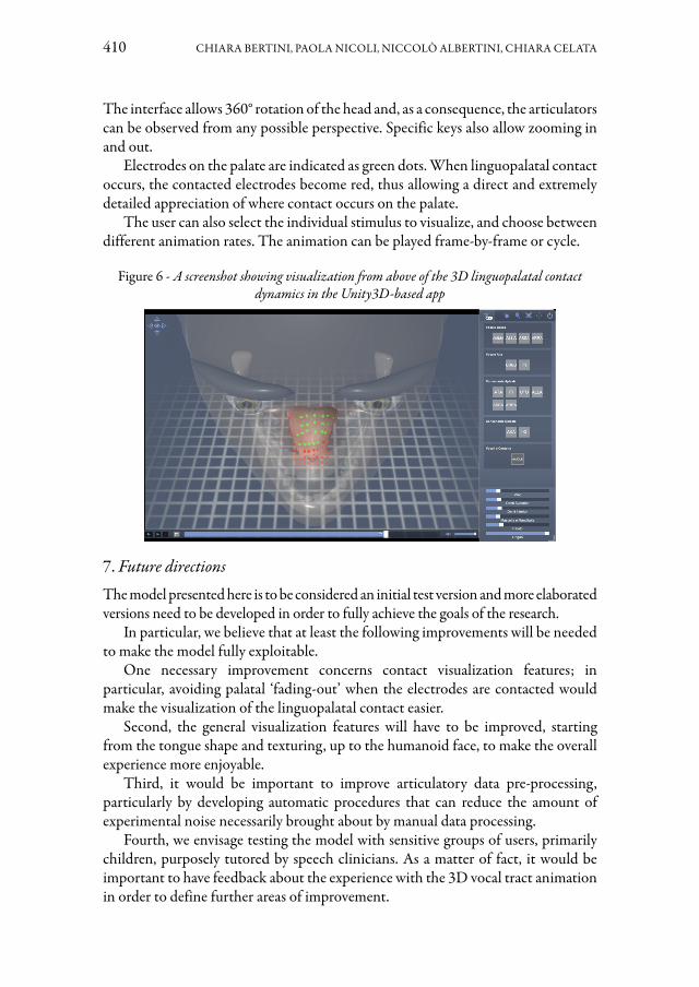
410 CHIARA BERTINI, PAOLA NICOLI, NICCOLÒ ALBERTINI, CHIARA CELATA
The interface allows 360° rotation of the head and, as a consequence, the articulators can be observed from any possible perspective. Specific keys also allow zooming in and out.
Electrodes on the palate are indicated as green dots. When linguopalatal contact occurs, the contacted electrodes become red, thus allowing a direct and extremely detailed appreciation of where contact occurs on the palate.
The user can also select the individual stimulus to visualize, and choose between different animation rates. The animation can be played frame-by-frame or cycle.
Figure 6 - A screenshot showing visualization from above of the 3D linguopalatal contact dynamics in the Unity3D-based app
7. Future directionsThe model presented here is to be considered an initial test version and more elaborated versions need to be developed in order to fully achieve the goals of the research.
In particular, we believe that at least the following improvements will be needed to make the model fully exploitable.
One necessary improvement concerns contact visualization features; in particular, avoiding palatal ‘fading-out’ when the electrodes are contacted would make the visualization of the linguopalatal contact easier.
Second, the general visualization features will have to be improved, starting from the tongue shape and texturing, up to the humanoid face, to make the overall experience more enjoyable.
Third, it would be important to improve articulatory data pre-processing, particularly by developing automatic procedures that can reduce the amount of experimental noise necessarily brought about by manual data processing.
Fourth, we envisage testing the model with sensitive groups of users, primarily children, purposely tutored by speech clinicians. As a matter of fact, it would be important to have feedback about the experience with the 3D vocal tract animation in order to define further areas of improvement.

A 3D MODEL OF LINGUOPALATAL CONTACT 411
Fifth, once the model will have reached a more elaborated technical specification, the speech corpus will have to be enlarged and a subset of speech phenomena will have to be targeted which could be of major interest with respect to relevant speech disorders / speech rehabilitation needs.
Sixth, the model is currently intended to work with a reference speaker compared to which patients and clinicians may evaluate individual speech production characteristics. This is related to the fact that EPG palates are currently custom-made for each user and therefore relatively expensive. The elaboration of second generation, smart and cheap EPG palates (Surace, 2016; Mat Zin, Md Rasib, Suhaimi & Mariatti, 2021) is expected to enlarge the applicability of the model also to individual patients’ production.
AcknowledgementsThis work was supported by Fondazione Pisa [grant 2016 “Disturbi motori nel parlato e biofeedback visivo: Simulare i movimenti articolatori in 3D” to Vincenzo Barone].
Bibliography
Bacsfalvi, P.C.E. (2007). Visual feedback technology with a focus on ultrasound: the effects of speech habilitation for adolescents with sensorineural hearing loss. PhD Dissertation, University of British Columbia.Barone, V. (2017-2020). Disturbi motori nel parlato e biofeedback visivo: Simulare i movimenti articolatori in 3D. Scuola Normale Superiore di Pisa, research project funded by Fondazione Pisa.Bernhardt, B., Bacsfalvi, P.C.E., Gick, B., Radanov, B. & Williams, R. (2005). Exploring the use of electropalatography and ultrasound in speech habilitation. In Journal of speech Language Pathology and Audiology, 29, 169-182.Celata, C., Vietti, A. & Spreafico, L. (2019). An articulatory account of rhotic variation in Tuscan Italian: Synchonized UTI and EPG data. In Gibson, M., Gil, J. (Eds.). Romance Phonetics and Phonology. Oxford (UK): Oxford University Press, 91-117.Chen, C., Celata, C. & Ricci, I. (2017). An EPG + UTI study of syllable onset and coda coordination and coarticulation in Italian. In Bertini, C., Celata, C., Meluzzi, C., Lenoci, G. & Ricci, I. (Eds.). Fattori sociali e biologici nella variazione fonetica – Social and biological factors in speech variation. Milano: Officinaventuno, 151-172.Gerard, J.-M., Perrier, P. & Payan, Y. (2006). 3D biomechanical tongue modeling to study speech production. In Harrington, J., Tabain, M. (Eds.). Speech Production: Models, Phonetic Processes, and Techniques. New York: Psychology Press, 85-102.Harper, J. (2012). Mastering Autodesk 3ds Max 2013. Hoboken (New Jersey): John Wiley & Sons.Katz, W., Campbell, T., Wang, J., Farrar, E., Coleman Eubanks, J., Balasubramanian, A., Prabhakaran, B. & Rennaker, R. (2014). Opti-Speech: A

412 CHIARA BERTINI, PAOLA NICOLI, NICCOLÒ ALBERTINI, CHIARA CELATA
real-time, 3D visual feedback system for speech training. In Proceedings of Interspeech 2014, Singapore, 1174-1178.Katz, W., McNeil, M. & Garst, D. (2010). Treating apraxia of speech (AOS) with EMA-supplied visual augmented feedback. In Aphasiology, 24, 826-837.Lloyd, J.E., Stavness, I. & Fels, S. (2012). ArtiSynth: A fast interactive biomechanical modeling toolkit combining multibody and finite element simulation. In Payan, Y. (Ed.) (2012). Soft Tissue Biomechanical Modeling for Computer Assisted Surgery. Studies in Mechanobiology, Tissue Engineering and Biomaterials, vol 11. Berlin/Heidelberg: Springer, 355-394.Mat Zin, S., Md Rasib, S.Z., Suhaimi, F.M. & Mariatti, M. (2021). The technology of tongue and hard palate contact detection: a review. In BioMed Eng OnLine, 20, #17.Moschos, G., Nikolaidis, N., Pitas, I. & Lyroudia, K. (2011). A Virtual Anatomical 3D Head, Oral Cavity and Teeth Model for Dental and Medical Applications. In Czachórski, T., Kozielski, S. & Stańczyk, U. (Eds.) (2011). Man-Machine Interactions 2. Advances in Intelligent and Soft Computing, vol 103. Berlin/ Heidelberg: Springer, 197-206.Sebkhi, N., Desai, D., Islam, M., Lu, J., Wilson, K. & Ghovanloo, M. (2017). Multimodal Speech Capture System for Speech Rehabilitation and Learning. IEEE transactions on bio-medical engineering, 64(11), 2639–2649.Spreafico, L., Celata, C., Vietti, A., Bertini, C. & Ricci, I. (2015). An EPG+UTI study of Italian /r/. In The Scottish Consortium for ICPhS 2015 (Ed.) (2015). Proceedings of the 18th International Congress of Phonetic Sciences. The University of Glasgow, paper no. 775.Surace, E. (2016). Design e sviluppo di un elettropalatografo per la valutazione dell’articolazione della parola realizzato con materiali piezoresistivi flessibili. Tesi di laurea magistrale, Università di Pisa & Scuola Superiore Sant’Anna.Wrench, A.A., Balch, P. (2015). Towards a 3D Tongue model for parameterising ultrasound data. In The Scottish Consortium for ICPhS 2015 (Ed.) (2015). Proceedings of the 18th International Congress of Phonetic Sciences. The University of Glasgow.

DOI: 10.17469/O2108AISV000022
CLAUDIO ZMARICH, ANNAROSA BIONDI, SERENA BONIFACIO, MARIA GRAZIA BUSÀ, BENEDETTA COLAVOLPE, MARIAVITTORIA GAIOTTO, FRANCESCO OLIVUCCI
Coarticulation and VOT in an Italian child from 18 to 48 months of age
This study brings new data to two understudied topics in Italian child language development: VOT and anticipatory C-V coarticulation. One female subject was recorded every three months from 18 to 48 months, while interacting with the clinician in front of some toys, repeating several times each bisyllabic pseudo-word beginning with voiceless and voiced stops. The acoustic signals were annotated using Praat and scripts were created for the automatic extraction of VOT and F2 values (Hz) for the Locus of Equations methods. RESULTS: Voiced stops appeared more difficult to produce than voiceless stops, but voicing contrast was finally achieved from 30 months of age. The degree of coarticulation increased with age, but at 48 months bilabials and alveolars were still less coarticulated than in adults.
Keywords: VOT acquisition, Anticipatory Coarticulation development, Acquisition of Italian, Acoustic analysis, Locus Equations.
1. IntroductionOver the past decades linguistic theories and theories of speech motor control have proceeded separately. This has been due to both theoretical and methodological reasons. From the theoretical point of view, there has been a pervasive influence of Generative Grammar, claiming that language and performance are separate, and language systems are often regarded as developing independently from other cognitive and sensorimotor systems (see Fodor, 1983; for a developmental perspective, see Redford, Oh, 2017). Methodologically, it has been difficult to trace neurobiological markers of the interaction between language and sensorimotor systems; this has been accompanied by an apparent lack of one-to-one correspondences between linguistic units and measures of executive behavior (see Smith, 2010; Laganaro, 2019). Traditional explanations in Linguistics have emphasized the acquisition of phonology, lexicon and morphosyntax, but not the acquisition of motor processes related to speech production (Goffman, 2015). The interconnection between linguistic and motor factors in the phonetic development is made complex by the continuous changes in the anatomo-physiological structures (for morphology, size and muscle innervation) and in the neural substrate of cognition (Callan, Kent, Guenther & Vorperian, 2000). Yet the neural organization for sensorimotor and cognitive-linguistic aspects is highly interactive: for instance, behavioral evidence

414 C. ZMARICH, A. BIONDI, S. BONIFACIO, M.G. BUSÀ, B. COLAVOLPE, M. GAIOTTO, F. OLIVUCCI
shows a high degree of co-occurrence between cognitive-linguistic deficits and motor deficits (Goffman, 2015; McAllister-Byun, Tessier, 2016), and theoretical proposals linking together language planning, speech motor control, and neurophysiological organization are currently available. According to Redford (2019), these proposals can be assigned to one of the two main existing frameworks: the Information-Processing Approach (DIVA model, Guenther, 1995; State Feedback Model, Parrell, Houde, 2019) and the Ecological Dynamics Approach (Task Dynamics, Saltzman, Munhall, 1989). When these two approaches were adapted into a developmental perspective, they inherited the preference for the basic units of speech representation and processing that were proper of the original models based on the adults’ speech production, i.e. the segment, for the Information-Processing Approach (Guenther, Vladusich, 2012) and the word, for the Ecological Dynamics Approach (Best, Goldstein, Nam, & Tyler, 2016).
In order to study the acquisition of motor control in early stages of language development, empirical analyses preferably rely on acoustic data, since acoustic analysis offers the possibility to quantify the phonetic continuum in the time-frequency domain, and to derive information – by inference – on the underlying movements. Until a generation ago, only acoustic analysis could be used to infer physiological processes; however, in recent years new technology and methods have been developed for the analysis of physiological processes, which are non-invasive and compatible with the analysis of evolutionary subjects (Goffman, 2015), although they can be used only from the subjects’ fourth year of age. Among these, the most successful ones are the Ultrasound Tongue Imaging-UTI (Abakarova, Iskarous & Noiray, 2018; Noiray, Abakarova, Rubertus, Krüger & Tiede, 2018; Zarkhova, 2018; Noiray, Wieling, Abakarova, Rubertus & Tiede, 2019a; Noiray, Popescu, Killmer, Rubertus, Krüger & Hintermeier, 2019b; Barbier, Perrier, Payan, Tiede, Gerber, Perkell & Menard, 2020; Cychosz, Munson & Edwards, 2021) and Optical-tracking devices like the Optotrack (Stone, 2012), which have sometimes been combined together. Nonetheless, some fields of inquiry in acquisition studies, namely Voice Onset Time (VOT) and the development of anticipatory coarticulation, have been shown to be easy to investigate by means of acoustic analysis only, thanks to the relatively clear and linear relation between speech movements and acoustic effects (Kent, Kim, 2008; Harrington, 2010; for VOT, see Grigos, Saxman & Gordon, 2005; Solé, 2018, as well as the contributions in the special number the of Journal of Phonetics devoted to VOT and edited by Cho, Whalen & Docherty, 2019; for anticipatory coarticulation, see Iskarous, Fowler & Whalen, 2010; Lindblom, Sussman, 2012). Last but not least, acoustic analysis is non-invasive, inexpensive and relatively simple to perform, and becomes the most viable solution for collecting and analysing huge amounts of data.

COARTICULATION AND VOT IN AN ITALIAN CHILD 415
2. Aims of this studyThe present investigation aims to contribute with experimental data, by means of acoustical analysis, to two topics in Italian child language development, namely the acquisition of VOT and the development of anticipatory CV coarticulation. These topics have been thoroughly studied in other western languages such as English, Spanish or French (see, respectively, Macken, Barton, 1980a; Eilers, Oller & Benito-Garcia, 1984; Allen, 1985, for VOT; and Sussman, Duder, Dalston & Cacciatore, 1999, for anticipatory coarticulation in American English), but rarely investigated in Italian, a so-called “true voicing language” (for VOT, see Bortolini, Zmarich, Fior, & Bonifacio, 1995; Zmarich, Bortone, Vayra & Galatà, 2013; for coarticulation, see Petracco, Zmarich, 2006; Zmarich et al., 2013).
2.1 The acquisition of VOT
The best parameter for quantifying and classifying voicing contrasts is VOT, which measures the time elapsed from the release of the consonant occlusion to the beginning of the vibration of the vocal folds. VOT provides an inferential estimate of speech motor control, requiring fine motor coordination of the respiratory, phonatory and articulatory structures. Early in phonetic development the voiced and unvoiced consonants tend to be realized as voiceless unaspirated, which allows for the synchronization between glottal and supraglottal events. It is only after the acquisition of additional articulatory manoeuvres that children come to achieve all the VOT categories that characterize their native language (see below). In different languages the phonemic contrast between sonority categories corresponds to distinct temporal intervals along the VOT continuum. Extensive cross-language studies (Abramson, Whalen, 2017; Cho, Whalen & Docherty, 2019) have shown that three categories of stops, having a rough correspondence across languages, emerge along the VOT continuum:1. “voicing lead”: characterised by negative VOT values, ranging from about -125
to -75 ms. Italian voiced stops belong to this category.2. “short voicing lag”: characterised by positive VOT values, ranging from 0 to +30
ms. Italian voiceless stops and English voiced stops belong to this category.3. “long voicing lag”: characterised by highly positive VOT values, ranging from
+60 to +100 ms. English voiceless stops belong to this category.Languages make use of these categories by having particular mean and range VOT values (Cho, Whalen & Docherty, 2019). Although many languages select only two among these voicing categories, there are languages which make use of more than two categories: among the languages with three-way contrasts are Thai, Vietnamese, Khmer; among the languages with more than three-way contrasts are Urdu, with a four-way contrast, and Sindhi with a five-way contrast. In fact, VOT is by no means the only mechanism available to languages for contrasting voicing: Cho et al. (2019) report other phonetic dimensions contributing to voicing contrast, such as consonant-induced F0 and voice quality.

416 C. ZMARICH, A. BIONDI, S. BONIFACIO, M.G. BUSÀ, B. COLAVOLPE, M. GAIOTTO, F. OLIVUCCI
VOT values have also been shown to depend on the specific stop and following-vowel sequence, due to aerodynamic reasons (Rothenberg, 1968): duration increases gradually as vowel openness decreases and the constriction for the plosive moves farther back in the vocal tract.
From a developmental point of view, in short lag/long lag VOT languages such as English, the acquisition of VOT contrast is usually accomplished earlier than in short lag/long lead languages such as Spanish, French and Arabic (Allen, 1985). Children acquire the short lag/long lag contrast around the age of 2;0 (Macken, Barton, 1980b). In languages that have VOT contrasts with short lag/long lead similar to that of Italian, children develop VOT contrasts around the age of 4;0 (Allen, 1985; Eilers et al., 1984; Al-Tamimi, Tarawneh & Howell, 2021).
2.2 The development of coarticulation
Acoustic analysis is also useful for the study of coarticulation, which refers to the temporal overlap of gestures belonging to neighbouring phones (Hardcastle, Hewlitt, 2006; Farnetani, Recasens, 2010). In a detailed survey, Mildner (2018) explains that coarticulatory phenomena can be originated by both biomechanical and linguo-specific factors. Coarticulation is the result of a continuous modification and adaptation of articulation to the linguistic context. First, this is a function of the biomechanical constraints of the phono-articulatory system for speech motor control, which are supposed to be universal – since they are biologically determined. Secondly, modification and adaptation are related to linguo-specific factors, because central planning and organization processes are governed by linguistic rules that differ depending on the speaker’s language. While carryover coarticulation has been mainly explained as a result of articulatory inertia, thus mantaining a universal character, anticipatory coarticulation, which is under the lens of the present research, has a cognitive basis, because it must be planned in advance, and it mantains a linguo-specific character. The development of coarticulation is a very debated issue (Noiray et al., 2019a), but general consensus has been reached now on the fact that young children generally coarticulate more than adults. A number of explanations have been offered for the greater children’s coarticulation, including:
(1) low-level pressures upon speech due to the protracted development of domain-general fine motor control, (2) the phonological reorganization of speech from more holistic units, such as syllables, into phonemes, (3) cognitive pressures from children’s limited working memory and speech planning capacities, (4) children’s inexperience articulating the sounds and words of their native language(s), or (5) a combination of these explanations (Cychosz et al., 2021: 367).
Recently, other factors have been discovered that possibly contribute to the acquisition of the degree of anticipatory coarticulation characterising adults’ productions: increase in phonological awareness, vocabulary size (Noiray et al., 2019b; Cychosz et al., 2021) and degree of speech practice (Cychosz et al., 2021). All these factors contribute to lower the coarticulation degree, by separating the articulation of the consonant from that of the following vowel.

COARTICULATION AND VOT IN AN ITALIAN CHILD 417
According to Noiray et al. (2019a), the three main hypotheses on the development of coarticulation are:a. “Holistic Approach”b. “Segmental Approach”c. “Gestural Hypotesis”According to the “Holistic Approach” in the first phase coarticulation units would be large, the articulators’ movements would be interdependent (Nittrouer, Studdert-Kennedy & Neely, 1996), and lexical development would have an important role in defining which combinations the child is able to achieve with coarticulation (Vihman, Velleman, 1989). Therefore, large units with interdependence of movements would shrink, and show an even greater motor independence of each articulator to achieve new segment combinations.
The “Segmental Approach” hypothesis could be considered as the exact opposite of the “Holistic Approach”. Initially, the articulatory movements to produce consonants and vowels would be independent of each other, and the first articulatory skills would manifest themselves in the realization of individual segments. Subsequently, depending on motor maturation and the increase in cohesion between movements, coarticulation over segments would develop. According to this hypothesis, thanks to the incremental maturation of the motor control of each articulatory organ, the precision and spatial-temporal coordination between segments would also improve (Kunhert, Nolan, 1999).
Finally, the “Gestural Hypotesis” refers to the coarticulation models developed starting from the Articulatory phonology theory of Browman, Goldstein (1992). Based on a concept of coarticulatory gesture that extends over the phonological segment, the development of coarticulation would depend on the degree of coarticulation compatibility of each gesture. The coarticulatory organization would take place in a more holistic or segmental way depending on whether the articulatory organs necessary to carry out the adjacent articulatory gestures compete with each other or not.
According to the most important studies on anticipatory coarticulation using the Locus Equations’ method (Sussman et al., 1992; Sussman et al., 1999; see also Gibson, Ohde, 2007), in the development of anticipatory coarticulation in a CV syllable the child progressively narrows the domain of the articulatory organization from the syllable to the individual C and V gestures, with the consequence that coarticulation decreases and phonemic distinctiveness increases. But the process is not linear and strongly depends on the physiological constraints on the articulators. The studies by Sussman and colleagues are important because they are among the first and the few to have investigated, with the use of acoustic analysis, the development of coarticulation starting from the beginning of babbling (at seven months of age), while the lowest age investigated using UTI devices starts from the fourth year.
As claimed by Sussman and colleagues, anticipatory coarticulation varies according to the articulatory place of the consonant. In the case of bilabial consonants, the articulation of the lips for the production of the consonant in a CV syllable is not

418 C. ZMARICH, A. BIONDI, S. BONIFACIO, M.G. BUSÀ, B. COLAVOLPE, M. GAIOTTO, F. OLIVUCCI
affected by the tongue dorsum during the production of the following vowel; this allows for maximum temporal overlap of the articulators (coarticulation as co-production). As for dental\alveolar consonants, the child must learn to differentiate and coordinate the tip (for the consonant) and the dorsum of the tongue (for the vowel), which are largely independent. As for velar consonants, the biomechanical constraints are the largest (both C and V are articulated with the tongue dorsum), and in this case the child must learn to mutually adapt the articulatory places for C and V (coarticulation as mutual adaptation).
2.3 Experimental hypotheses
It is well-established that it is difficult to produce vocal fold vibration during voiced stops due to challenging aerodynamic conditions. Ohala (2011: 64) described the existence of an “Aerodynamic Voicing Constraint” [...]:
voicing requires a sufficient airflow through the adducted vocal cords. The airflow requires a sufficient pressure difference (ΔP) between subglottal pressure (Ps) and oral pressure (Po). During an obstruent air accumulates in the oral cavity thus increasing Po. When the Po approaches Ps, the airflow falls below that needed for vocal cord vibration and thus voicing is extinguished.
Speakers of languages like Italian where voiced stops require laryngeal vibration may need some articulatory adjustments, used singly or in combination, to limit the increase of oral pressure and thus achieve the pressure differential for voicing initiation. Such articulatory adjustments are: oral leak, nasal leak (i.e., releasing airflow through an incomplete velopharyngeal closure), larynx lowering, tongue root advancement (Rothenberg, 1968; Westbury, 1983). Among these adjustments, only the larynx lowering, and maybe the tongue root advancement, could guarantee the achievement of the perceptual effect of voicing without introducing collateral effects such as nasalisation, frication or vowel epenthesis. The presence of consistent percentages of segment productions that are nasalized or preceded by a schwa-like vowel in adult speakers of true voicing languages like French or Spanish (Solé, 2018) is explainable with perceptual considerations that are not investigated here.
Developmental studies on the acquisition of voicing in languages with voiced stops with negative VOT values show that two-year-old children have still not acquired the VOT values for initial voiced stops (for Spanish: Macken, Barton, 1980b; Eilers et al., 1984; for French: Allen, 1985; for Jordanian Arabic: Al-Tamimi et al., 2021). Italian data from Zmarich et al. (2013) confirm this difficulty for some children even at the beginning of the fourth year of age. If the acquisition criteria are the attainment of mean and standard deviation of adult values for consonant place of articulation and vocalic context (see Fig. 1, from Bortolini et al., 1995; see also Esposito, 2002), then most of the children in Zmarich et al. (2013) are still far from target values.
On the basis of both literature results and our previous investigations, the present study aims to test the following working hypotheses:

COARTICULATION AND VOT IN AN ITALIAN CHILD 419
1. VOT: Since the production of initial voiced stop consonants requires some larynx-external mechanism in order to sustain an adequate transglottal pressure drop during stop closure (as an active lowering of the glottis), children will be more advanced in the acquisition of appropriate VOT values for voiceless than for voiced consonants.
Figure 1 - VOT values as produced by Italian adults ( from Bortolini et al., 1995)
2. Anticipatory coarticulation: While the coarticulation degree decreases with age, children will not be able to organize consecutive articulatory gestures with a uniform organization scheme (e.g., segmental or syllabic) (Noiray et al., 2018). Instead, coarticulatory organization will be subjected to different articulatory constraints according to Sussman et al. (1999) and sensitive to the underlying articulatory properties of the combined segments (different lingual coarticulatory resistance and aggressiveness for consonants and vowels according to the DAC model). The model predicts that “the size, temporal extent, and direction of lingual coarticulation are conditioned by the severity of the requirements imposed on the tongue for the production of vowels and consonants” (Farnetani, Recasens, 2010: 340). Criteria for acquisition are the attainment of mean adult coarticulation values, as indexed by the Locus Equations (LE, see Lindblom, 1963; Krull, 1989). A LE describes a 1st order regression fit to a scatter of vowel steady-state frequency values predicting the onset of F2 transition values in CV sequences with a fixed C, of the form F2cons = k * F2vow + c. This measure provides an overall estimation of coarticulation, provided that LE slopes (indexed by k values) be calculated on CV sequences with vowel pooling and voiced stops (Tabain, 2000). A nice characteristic of this method consists in an intrinsic normalization of k values, which could vary between 0

420 C. ZMARICH, A. BIONDI, S. BONIFACIO, M.G. BUSÀ, B. COLAVOLPE, M. GAIOTTO, F. OLIVUCCI
(no coarticulation at all) and 1 (maximal coarticulation), allowing the direct comparison of the productions by children at different ages to those by adults. Petracco, Zmarich (2006) established the following values for k, averaged over the productions of four Italian adults (see Fig. 2, from Petracco, Zmarich, 2006). We also report the magnitude of R2, which in the regression analysis is used to indicate the fraction of variance of the dependent variable scores explained by the independent variable scores:a. Bilabials: k = 0.915, R2 = 0.973b. Dentals: k = 0.790, R2 = 0.952c. Velars: k = 0.989, R2 = 0.983
The work presented here is exploratory in nature, aiming to: (i) review the state of the art on VOT acquisition and coarticulation development; (ii) present a theoretical frame with which to formulate the experimental hypotheses and the appropriate methods for future investigations; and (iii) apply these methods to investigate one subject in a longitudinal design, thus keeping aside, for the moment, potentially complicating questions like individual variability.
3. Subjects and MethodsThis individual case study is part of a longitudinal corpus of ten children collected with the aim to investigate Italian children’s speech development. The study uses data from both the phonetic transcription of segments and the acoustic analysis of speech. The subjects were recruited by one of the authors (S. Bonifacio) in Trieste (Italy) from 2007 to 2009, in two kindergartens. The parents compiled the MacArthur CDI survey for their children’s lexical productions (“Primo Vocabolario del Bambino”, Caselli, Pasqualetti & Stefanini, 2007) and filled out a questionnaire reporting information on normal psycho-physical development and monolingual (Italian) language development. All the parents signed an informed consent form. When children were 18-months old, they underwent auditory screening (Ling Six Sound Test, Ling, 1976) to exclude the presence of hearing impairments.

COARTICULATION AND VOT IN AN ITALIAN CHILD 421
Figure 2 - Diagram distribution of pairs of F2onset and F2vowel values (Hz) relative to syllables p/bV (top), t/dV (middle), k/gV (bottom) produced by the four adult subjects
in Petracco, Zmarich (2006). The points within each diagram are interpolated by the regression line, whose equation is reported at the bottom
The children were recorded every month from 18 to 24 months, and then every three months from 24 to 48 months. The session organization was semi-structured (Schmitt, Meline, 1990), with the child interacting with the clinician in front of a set of toys. The objects were chosen based on the list of words compiled by the parent on the MacArthur CDI. In order to conduct a study on the development of VOT, in addition to saying “common” words, children were invited to repeat each of the 12 VOT test items at least three times, immediately after they were uttered by the third author. The test items were the following minimal pair pseudo-words, all stressed on the first syllable, and contrasting labial, dental and velar voiced and voiceless stops: papa, baba, pipi, bibi, tata, dada, titi, didi, kaka, gaga, kiki, gigi. Each recording session lasted on average about one hour. Once the session was over, the sample of language collected at 18 and 21 months was considered valid and representative of the child’s linguistic abilities only if the number of lexical forms produced represented at least 50% of the words in the lexical list compiled by the parent. All the recordings are available in digital format (.wav) at a rate of 44.1 kHz

422 C. ZMARICH, A. BIONDI, S. BONIFACIO, M.G. BUSÀ, B. COLAVOLPE, M. GAIOTTO, F. OLIVUCCI
and 16 bit (Edirol R-09 by Roland). SC is a female child. When she was 18-months old she was credited with a vocabulary of 120 words by their parents (through CDI), and then she spontaneously produced more than 50% of the words in the lexical list compiled by the parent during the first session. For statistical reasons, we chose to add to stage one also the speech productions from the 19th month of age. From there onwards, the sessions we chose to analyse for the present contribution concern the 24, 30, 36, 42 and 48 months of age, i.e., every 6 months. The acoustic files were annotated using Praat (Boersma, Weenink, 2021) with TextGrids (see Fig. 3).
Figure 3 - Example of a typical Praat display as used in this study
For each file, all the productions containing CV or CVC syllabic structures where C was a stop consonant were selected. If the words were not isolated, we segmented and labelled also all other words in the utterance. As for segmentation, we followed the conventions proposed by Salza (1990). For voiced consonants, the boundaries marking the consonant beginning and the vowel beginning (where the burst separates the consonant from the following vowel) were used for the measurement of the VOT interval. For voiceless consonants VOT was measured from the burst, representing the beginning of VOT, up to the vowel onset. The voiceless stop beginning a new utterance was credited with a duration interval of 150 ms before the burst, a conventional value based on previous determination of the average duration of intervocalic voiceless stops in Italian children of the same age.
Children are often expected to misproduce the phonetic shape of target words (with respect to the adult pronunciation). This is due to a number of reasons including: the presence of so-called phonological processes; phonetic phenomena resulting from informal connected speech; voicing errors; other phenomena described later. Thus, individual target and actual C and V segments were labelled in

COARTICULATION AND VOT IN AN ITALIAN CHILD 423
separate tiers using SAMPA symbols. The syllable status as to lexical stress, position in the word and style of production (spontaneous or repeated) were categorized. Clitics were considered a part of prosodic words. Finally, a number of exogenous events (like noise or uncertain transcriptions) or endogenous events, like a number of phonological processes (sometimes related to the production of voicing), altering the syllable target, were also categorized (see later).
All annotations were done by one of the authors (mostly, but not always, M. Gaiotto, as part of her MA thesis). Other annotations were done by B. Colavolpe. Both annotators were Linguistics students at the University of Padova and, at the same time, speech therapists working with children. They had attended an internship at ISTC-CNR1 under the tutoring of the first author, where they practiced with the methods employed in this study, following a written protocol continually updated and discussing problematic cases with the first author. All of their textgrids were checked by the first author, and, if necessary, corrected and integrated. A number of ambiguous cases were left out. A Praat script developed by one of the authors (F. Olivucci) was used to extract the VOT values (ms). For all the vowels in the annotated textgrid, the script extracts the values for the calculation of coarticulation, i.e., F1 and F2 values in a number of points along the vowel, including the middle. For consonants, the F2 values at the beginning of the formant transition are calculated. The algorithm was designed so as to extract the optimal formants for each vowel as well as the parameters change as a function of the vowel position in the vowel quadrilateral. Vowels are then divided accordingly into 3 macrocategories.
The script produced a .csv file, which allowed to obtain a number of other variables as a result of operations among the columns of the matrix, yielding the duration values of segments and syllables. In this way it was possible to estimate speech rate (not considered here) and, most importantly, to exclude syllables characterized by VOT values greater than +15 ms for the coarticulation analysis, that is, only the syllables characterized by a negative VOT interval or a positive VOT interval lower than 16 ms were selected. Only syllables preceded by silence (equal to or greater than 250 ms) were used for the VOT analysis, as this context is considered the most challenging for speakers of languages, like Italian, that produce voiced stops by means of negative VOT (i.e., with true voicing, see Ohala, 2011; Solé, 2018).
As for anticipatory coarticulation, it was measured by means of Locus Equations (LE, see Lindblom, 1963; Krull, 1989). As described above, a LE describes a 1st order regression fit to a scatter of vowel steady-state frequency values predicting the onset of F2 transition values in CV sequences with a fixed C, of the form F2cons = k * F2vow + c.
Regression analysis is a statistical procedure that describes the relation between two variables: a dependent one, which in this case corresponds to the consonant F2 value; and an independent one, which corresponds to the vowel F2 values, the aim being to analyze how the consonant value changes as the vowel value varies. When
1 Istituto di Scienze e Tecnologie della Cognizione – CNR, Padova, Italy.

424 C. ZMARICH, A. BIONDI, S. BONIFACIO, M.G. BUSÀ, B. COLAVOLPE, M. GAIOTTO, F. OLIVUCCI
doing regression analysis, the Systat software for statistical analysis also calculates, among other things, the values of 4 parameters that are useful for the present study:1. k: indicates the slope of the regression line, describing the anticipatory
coarticulation degree of the vowel on the consonant;2. c: the intersection of the regression line on the y axis; it thus corresponds to the
value assumed by the dependent variable when the independent variable (x) is equal to 0; Iskarous, Fowler & Whalen (2010) suggest that this parameter is directly related to the degree of involvement of the body of the tongue in the realization of the constriction for the consonant production.
3. R2: indicates the determination coefficient, which measures the variance fraction, that is the amount of variance of the dependent variable as accounted for by the independent variable.
4. SEE: the standard error of estimate is a variability index measuring the distance of the data points from the regression line.
4. ResultsThe number of CV and CVC syllables beginning with a stop consonant produced by SC and constituting the database for the present work is 3255. The presentation of the results will be organized around three main points, following a longitudinal perspective: (1) a qualitative analysis of the relative frequency of the type of endogenous and exogenous processes (see Tab. 1) which altered the potential consonant targets up to their exclusion from further analyses. This investigation becomes particularly interesting when we focus on the utterance-initial syllables as a particularly challenging position for the production of voiced consonants; (2) a statistical analysis of the VOT values for voiced and voiceless targets realized in the absence of processes; (3) a statistical calculation of the degree of anticipatory coarticulation for each of the three main places of articulation, pooling together initial and non-initial syllables (only those with a VOT value lower than 15 ms, see later).
Table 1 - Types of endogenous and exogenous processes (see text for explanations)
1 Saturated signal2 Weak signal3 Noised signal4 Unidentified target5 Uncertain transcription6 Breathy voice7 Creaky voice8 Whispered9 Ejectivisation (stop realized in an ejective pneumatic modality)
10 Diphthongization 11 Vowel Epenthesis (oral leakage)12 Consonant Epenthesis
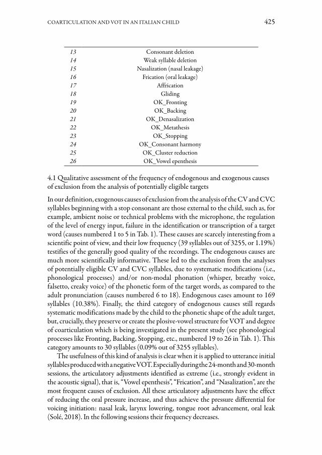
COARTICULATION AND VOT IN AN ITALIAN CHILD 425
13 Consonant deletion14 Weak syllable deletion15 Nasalization (nasal leakage)16 Frication (oral leakage)17 Affrication18 Gliding19 OK_Fronting20 OK_Backing21 OK_Denasalization22 OK_Metathesis23 OK_Stopping24 OK_Consonant harmony25 OK_Cluster reduction26 OK_Vowel epenthesis
4.1 Qualitative assessment of the frequency of endogenous and exogenous causes of exclusion from the analysis of potentially eligible targets
In our definition, exogenous causes of exclusion from the analysis of the CV and CVC syllables beginning with a stop consonant are those external to the child, such as, for example, ambient noise or technical problems with the microphone, the regulation of the level of energy input, failure in the identification or transcription of a target word (causes numbered 1 to 5 in Tab. 1). These causes are scarcely interesting from a scientific point of view, and their low frequency (39 syllables out of 3255, or 1.19%) testifies of the generally good quality of the recordings. The endogenous causes are much more scientifically informative. These led to the exclusion from the analyses of potentially eligible CV and CVC syllables, due to systematic modifications (i.e., phonological processes) and/or non-modal phonation (whisper, breathy voice, falsetto, creaky voice) of the phonetic form of the target words, as compared to the adult pronunciation (causes numbered 6 to 18). Endogenous cases amount to 169 syllables (10.38%). Finally, the third category of endogenous causes still regards systematic modifications made by the child to the phonetic shape of the adult target, but, crucially, they preserve or create the plosive-vowel structure for VOT and degree of coarticulation which is being investigated in the present study (see phonological processes like Fronting, Backing, Stopping, etc., numbered 19 to 26 in Tab. 1). This category amounts to 30 syllables (0.09% out of 3255 syllables).
The usefulness of this kind of analysis is clear when it is applied to utterance initial syllables produced with a negative VOT. Especially during the 24-month and 30-month sessions, the articulatory adjustments identified as extreme (i.e., strongly evident in the acoustic signal), that is, “Vowel epenthesis”, “Frication”, and “Nasalization”, are the most frequent causes of exclusion. All these articulatory adjustments have the effect of reducing the oral pressure increase, and thus achieve the pressure differential for voicing initiation: nasal leak, larynx lowering, tongue root advancement, oral leak (Solé, 2018). In the following sessions their frequency decreases.

426 C. ZMARICH, A. BIONDI, S. BONIFACIO, M.G. BUSÀ, B. COLAVOLPE, M. GAIOTTO, F. OLIVUCCI
4.2 VOT acquisition
Before running the statistical analysis, we eliminated all the child’s productions of the utterance-initials CV and CVC stop targets which were affected by any of the exogenous or endogenous processes listed in Tab. 1, with the exception of the processes numbered 18 to 26, which preserved the nature of plosive consonants. For statistical reasons, and for the sake of simplicity, in order to be able to represent the phonological sonority contrast for all the sessions, here we pooled together all the initial CV and CVC syllables regardless of the vowel (all possible vowels, but with a prevalence of [a], and [i]), the “lexical stress” status (stressed or unstressed syllable), or the style of production (spontaneous vs. repeated). A series of separated t-student tests was then performed in order to assess the significance of the voicing contrast at each session.
Figure 4 - Sampling distributions and box plots of the VOT values (s) for each age session, divided according to the voiced vs. voiceless nature of “adult” stop targets, for the bilabial place
of articulation
For each session and for each place of articulation, the child was able to produce a number of occurrences that was sufficient to allow statistical comparisons by means of the t-student test (which however is known to be quite robust to atypical sampling distribution), with the exception of the first session at 18 months of age, in which the child did not produce any phonologically voiced velar stop.
Fig. 4 plots the sampling distribution of the VOT values, divided according to the voiced vs. voiceless nature of “adult” stop targets, as produced by the child in each session, for the bilabial place of articulation. The SC productions at the 18- and 24-month sessions did not differ significantly for voicing, because of the production of voiced targets by means of positive VOT. The first significant

COARTICULATION AND VOT IN AN ITALIAN CHILD 427
difference was achieved at 30 months of age, when voiced and voiceless productions were produced with the mean (and SD) values of -0.072 s (0.060) and 0.014 s (0.009), respectively (t (12.5) = -5.137, p < 0.000).
Figure 5 - Sampling distributions and box plots of the VOT values (s) for each age session, divided according to the voiced vs. voiceless nature of “adult” stop targets, for the dental place
of articulation
From that time onwards, the child was able to maintain the voicing contrast, with a slight reduction of the negative VOT values at 48 months. The mean (and SD) values at the 48-month final stage were -0.105 s (0.041) for /b/, and 0.011 s (0.011) for /p/.
As for dental stops (Fig. 5), SC’s productions at the 18- and 24-month sessions did not differ significantly for voicing, mainly because of the production of voiced targets by means of positive VOT. The first significant difference was achieved at 30 months of age, when voiced and voiceless stops were produced with the mean values (and SD) of -0.098 s (0.075) and 0.015 s (0.006), respectively (t (23.5)=-11.113, p < 0.000). From that time onward, the child was able to maintain the voicing contrast, with a slight increase of the negative VOT values at 48 months. The mean (and SD) values at the 48-months final stage were -0.090 s (0.039) for /d/, and 0.021 s (0.013) for /t/.
As for velar stops (Fig. 6), at the initial session the child did not produce the voiced targets, and at 24 months of age her targets did not differ significantly for voicing, but at 30 months of age she appeared to be able to differentiate significantly voiced from voiceless targets, with the mean (and SD) values of -0.077 s (0.062) and 0.052 s (0.027) respectively (t (10.4)= -6.302, p < 0.000). From that time onward, she was able to maintain the voicing contrast, with a sharp increase in negative VOT values at 48 months and an important reduction in variability as compared to

428 C. ZMARICH, A. BIONDI, S. BONIFACIO, M.G. BUSÀ, B. COLAVOLPE, M. GAIOTTO, F. OLIVUCCI
the previous session. The mean (and SD) values at the 48 months final stage were -0.113 s (0.021) for /g/, and 0.046 (0.024) for /t/.
Figure 6 - Sampling distributions and box plots of the VOT values (s) for each age session, divided according to the voiced vs. voiceless nature of “adult” stop targets, for dental place
of articulation
4.3 Coarticulation development
Before running the statistical analysis, we eliminated all the child’s CV and CVC stops which were affected by any of the exogenous or endogenous processes listed in Tab. 1, with the exception of the processes numbered 18 to 26, which preserved the nature of plosive consonants.
As explained in section 2 above, we excluded all syllables with VOT values greater than +15 ms. The rationale behind this decision was that, if one wants to use the F2 value measured at the beginning of the formant transition as an acoustic index of the articulatory position of the tongue dorsum, one cannot allow the tongue to have the time to move away from the articulatory place of the occlusion (at least for dentals and velars). Ideally, one has to rely only on voiced consonants, but in this case one is at risk of statistical bias for the small amount of occurrences, especially during the first sessions.
Finally, we performed a series of linear regression analyses, separated for articulation place within any session. The frequency values (Hz) of the F2 transition sampled at its onset was the dependent variable, while the frequency of F2 when measured in the vowel nucleus was the independent variable.
We obtained a scatterplot fit with a linear regression line, the ‘locus equation,’ of the form F2cons = k *F2vow + c where k and c are the constants, slope and y-intercept, respectively (see also § 2.3).
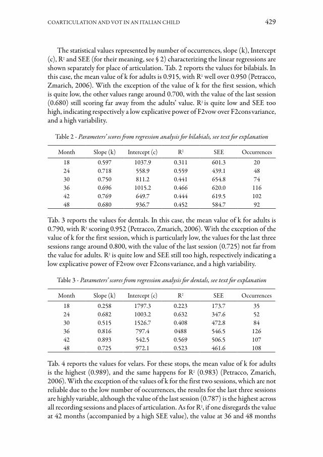
COARTICULATION AND VOT IN AN ITALIAN CHILD 429
The statistical values represented by number of occurrences, slope (k), Intercept (c), R2 and SEE (for their meaning, see § 2) characterizing the linear regressions are shown separately for place of articulation. Tab. 2 reports the values for bilabials. In this case, the mean value of k for adults is 0.915, with R2 well over 0.950 (Petracco, Zmarich, 2006). With the exception of the value of k for the first session, which is quite low, the other values range around 0.700, with the value of the last session (0.680) still scoring far away from the adults’ value. R2 is quite low and SEE too high, indicating respectively a low explicative power of F2vow over F2cons variance, and a high variability.
Table 2 - Parameters’ scores from regression analysis for bilabials, see text for explanation
Month Slope (k) Intercept (c) R2 SEE Occurrences
18 0.597 1037.9 0.311 601.3 2024 0.718 558.9 0.559 439.1 4830 0.750 811.2 0.441 654.8 7436 0.696 1015.2 0.466 620.0 11642 0.769 649.7 0.444 619.5 10248 0.680 936.7 0.452 584.7 92
Tab. 3 reports the values for dentals. In this case, the mean value of k for adults is 0.790, with R2 scoring 0.952 (Petracco, Zmarich, 2006). With the exception of the value of k for the first session, which is particularly low, the values for the last three sessions range around 0.800, with the value of the last session (0.725) not far from the value for adults. R2 is quite low and SEE still too high, respectively indicating a low explicative power of F2vow over F2cons variance, and a high variability.
Table 3 - Parameters’ scores from regression analysis for dentals, see text for explanation
Month Slope (k) Intercept (c) R2 SEE Occurrences
18 0.258 1797.3 0.223 173.7 3524 0.682 1003.2 0.632 347.6 5230 0.515 1526.7 0.408 472.8 8436 0.816 797.4 0488 546.5 12642 0.893 542.5 0.569 506.5 10748 0.725 972.1 0.523 461.6 108
Tab. 4 reports the values for velars. For these stops, the mean value of k for adults is the highest (0.989), and the same happens for R2 (0.983) (Petracco, Zmarich, 2006). With the exception of the values of k for the first two sessions, which are not reliable due to the low number of occurrences, the results for the last three sessions are highly variable, although the value of the last session (0.787) is the highest across all recording sessions and places of articulation. As for R2, if one disregards the value at 42 months (accompanied by a high SEE value), the value at 36 and 48 months
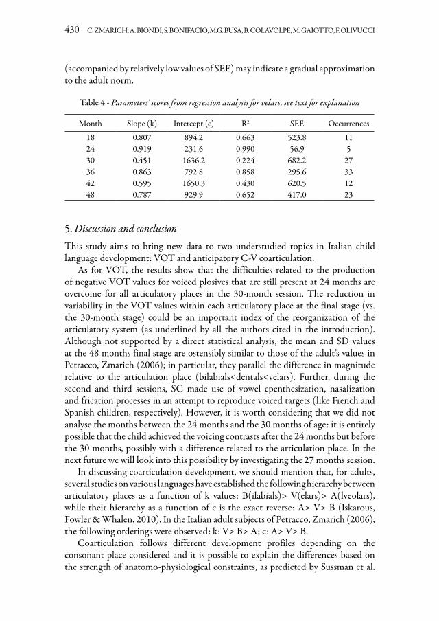
430 C. ZMARICH, A. BIONDI, S. BONIFACIO, M.G. BUSÀ, B. COLAVOLPE, M. GAIOTTO, F. OLIVUCCI
(accompanied by relatively low values of SEE) may indicate a gradual approximation to the adult norm.
Table 4 - Parameters’ scores from regression analysis for velars, see text for explanation
Month Slope (k) Intercept (c) R2 SEE Occurrences
18 0.807 894.2 0.663 523.8 1124 0.919 231.6 0.990 56.9 530 0.451 1636.2 0.224 682.2 2736 0.863 792.8 0.858 295.6 3342 0.595 1650.3 0.430 620.5 1248 0.787 929.9 0.652 417.0 23
5. Discussion and conclusionThis study aims to bring new data to two understudied topics in Italian child language development: VOT and anticipatory C-V coarticulation.
As for VOT, the results show that the difficulties related to the production of negative VOT values for voiced plosives that are still present at 24 months are overcome for all articulatory places in the 30-month session. The reduction in variability in the VOT values within each articulatory place at the final stage (vs. the 30-month stage) could be an important index of the reorganization of the articulatory system (as underlined by all the authors cited in the introduction). Although not supported by a direct statistical analysis, the mean and SD values at the 48 months final stage are ostensibly similar to those of the adult’s values in Petracco, Zmarich (2006); in particular, they parallel the difference in magnitude relative to the articulation place (bilabials<dentals<velars). Further, during the second and third sessions, SC made use of vowel epenthesization, nasalization and frication processes in an attempt to reproduce voiced targets (like French and Spanish children, respectively). However, it is worth considering that we did not analyse the months between the 24 months and the 30 months of age: it is entirely possible that the child achieved the voicing contrasts after the 24 months but before the 30 months, possibly with a difference related to the articulation place. In the next future we will look into this possibility by investigating the 27 months session.
In discussing coarticulation development, we should mention that, for adults, several studies on various languages have established the following hierarchy between articulatory places as a function of k values: B(ilabials)> V(elars)> A(lveolars), while their hierarchy as a function of c is the exact reverse: A> V> B (Iskarous, Fowler & Whalen, 2010). In the Italian adult subjects of Petracco, Zmarich (2006), the following orderings were observed: k: V> B> A; c: A> V> B.
Coarticulation follows different development profiles depending on the consonant place considered and it is possible to explain the differences based on the strength of anatomo-physiological constraints, as predicted by Sussman et al.

COARTICULATION AND VOT IN AN ITALIAN CHILD 431
(1999), and confirmed recently by many authors using the UTI technology (see for instance, Noiray et al., 2018, 2019a, 2019b, 2020).
The bilabial occlusion, not being anatomically binding for the tongue, would allow the largest temporal overlap of the two gestures, as occurs in adults, where the coarticulatory influence is greatest: at the time of release the tongue is already in the position for the vowel (coarticulation as an articulatory co-production). In the 18 months session, SC hardly shows coarticulation: the tongue is still in motion when the occlusion is released. From the subsequent session, independent movements of the tongue for the production of the vowel begin to be loosely timed with respect to the release. Once a first level of coordination is reached, it is maintained.
As for dentals, the child must learn to differentiate almost independently and coordinate the tip and the back of the tongue (anatomical constraints). In adults, coarticulation has little acoustic effects, since the tip of the tongue can theoretically remain stationary on the consonant place regardless of the position of the dorsum which articulates the vowel. In line with this hypothesis, at the 18-month session coarticulation is very low, then it increases, gradually approaching adults’ values.
In the case of velars, the biomechanical constraints are the largest (the consonant and the vowel use the same articulator, the tongue dorsum), and in the adult the acoustic effect shows a very high degree of coarticulation (as a reciprocal articulatory adaptation). In SC, after an initial period of variability, productions stabilize at relatively high values, which show a greater amount of coarticulation than the other place categories examined.
Trying to interpret the results with reference to the three hypotheses on coarticulation development put forward by Noiray et al. (2019a) and discussed in § 2.2 above, the present results are more in agreement with the Gestural Hypothesis, which predicts that coarticulatory organization takes place in either a holistic or segmental way depending on whether the articulatory organs necessary to carry out adjacent articulatory gestures compete with each other or not.
The limitations of the present study are many, and most of them are due to the single case design. Thus, this study cannot address basic questions in any developmental investigation, such as individual variability and the many factors behind this (gender, education, socio-economic conditions, etc...). In addition, the effect of important variables such as vocalic context and place of articulation for stops in VOT could not be statistically determined, due to the low statistical representativity, and we did not normalize for speech rate. Another direction for future investigations will be to submit to a perceptual judgement the productions affected by vowel epenthesization, nasalization and frication processes. In fact, we know after Solé (2018) that many adults’ voiced productions are affected by some process of that type, and nevertheless they are tolerated and considered acceptable instances of voiced productions. We hope that in future developments of this project, all these problems will be addressed as we will extend the investigation to all of the ten subiects in the “Trieste” children corpus.

432 C. ZMARICH, A. BIONDI, S. BONIFACIO, M.G. BUSÀ, B. COLAVOLPE, M. GAIOTTO, F. OLIVUCCI
Bibliography
Abakarova, D., Iskarous, K. & Noiray, A. (2018). Quantifying lingual coarticulation in German using mutual information: An ultrasound study. In The Journal of the Acoustical Society of America, 144(2), 897-907.Abramson, A.S., Whalen, D.H. (2017). Voice Onset Time (VOT) at 50: theorical and practical issues in measuring voicing distinctions. In Journal of Phonetics, 63, 77-86.Al-Tamimi F., Tarawneh, R., & Howell, P. (2021). Development of voice onset time in Arabic. In Lingua, 262, 103-117.Allen, G.D. (1985). How the young French child avoids pre-voicing problem for word-initial voiced stops. In Journal of Child Language, 12(1), 37-46.Barbier, G., Perrier, P., Pavan, Y., Tiede, M.K., Gerber, S., Perkell, J.S. & Menard, L. (2020). What anticipatory coarticulation in children tells us about speech motor control maturity. In Plos one, 15(4), e0231484.Best, C.T., Goldstein, L.M., Nam, H. & Tyler, M.D. (2016). Articulating what infants attune to in native speech. In Ecological Psychology, 28(4), 216–261.Boersma, P., Weenink, D. (2021). PRAAT: doing phonetics by computer. [Computer program], Version 6.1.40, retrieved 27 February 2021 from http://www.praat.org/.Bortolini, U., Zmarich, C., Fior, R. & Bonifacio, S. (1995). Word-initial voicing in the productions of stops in normal and preterm Italian infants. In International Journal of Pediatric Otorhinolaryngology, 31, 191-206.Browman, C.P., Goldstein, L. (1992). Articulatory Phonology: An Overview. In Phonetica, 49(3-4), 155-180.Callan, D.E., Kent, R.D., Guenther, F.H. & Vorperian H.K. (2000). An auditory-feedback-based neural network model of speech production that is robust to developmental changes in the size and shape of the articulatory system. In Journal of Speech, Language and Hearing Research, 43, 721-736.Caselli, M.C., Pasqualetti, P. & Stefanini, S. (2007). Parole e frasi nel Primo Vocabolario del Bambino. Milano: FrancoAngeli.Cho, T., Whalen, D.H. & Docherty G. (2019). Voice onset time and beyond: Exploring laryngeal contrast in 19 languages. In Journal of Phonetics, 72, 52-65.Colavolpe, B. (2020). Analisi acustica della coarticolazione anticipatoria CV: uno studio sperimentale longitudinale su bambini di età compresa tra i 18 e 48 mesi. Tesi di Laurea Magistrale, Università degli Studi di Padova.Cychosz, M., Munson, B. & Edwards, J.R. (2021). Practice and experience predict coarticulation in child speech. In Language Learning and Development, 17(4), 1-31.Eilers, E.R., Oller, D.K. & Benito-Garcia. C.R. (1984). The acquisition of the voicing contrast in Spanish and English learning infants and children: a longitudinal study. In Child Lang, 11(2), 313-336.Esposito, A. (2002). On vowel height and consonantal voicing effects: data from Italian. In Phonetica, 59, 197-231.

COARTICULATION AND VOT IN AN ITALIAN CHILD 433
Farnetani, E., Recasens, D. (2010). Coarticulation and connected speech processes. In Hardcastle, W.J., Laver J. & Gibbon F.E (Eds.), The Handbook of Phonetic Sciences: Second Edition. Hoboken (New Jersey): Blackwell Publishing, 316-352.Fodor, J.A. (1983). The Modularity of Mind. Cambridge (Massachussets): MIT Press.Gaiotto, M. (2020). L’acquisizione dell’opposizione di sonorità in bambini italiani: studio sperimentale sulle caratteristiche acustiche del Voice Onset Time. Tesi di Laurea Magistrale, Università degli Studi di Padova.Gibson, T., Ohde, R.N. (2007). F2 Locus Equations: Phonetic descriptors of coarticulation in 17-to 22-months-old children. In Journal of Speech, Language and Hearing Research, 50, 97-108.Goffman, L. (2015). Effects of language on motor processes in development. In Redford, M.A. (Ed.), The Handbook of Speech Production. Hoboken (New Jersey): Wiley Online Library, 555-577.Grigos, M.I., Saxman, J.H. & Gordon, A.M. (2005). Speech motor development during acquisition of the voicing contrast. In Journal of Speech in Language, and Hearing Research, 48(4), 739-752.Guenther, F.H. (1995). Speech sound acquisition, coarticulation, and rate effects in a neural network model of speech production. In Psychological Review, 102(3), 594.Guenther, F.H., Vladusich, T. (2012). A neural theory of speech acquisition and production. In Journal of Neurolinguistics, 25(5), 408-422.Hardcastle, W.J., Hewlett, N. (Eds.) (2006). Coarticulation: Theory, Data and Techniques. Cambridge (UK): Cambridge University Press.Harrington, J. (2010). Acoustic phonetics. In Hardcastle, W.J., Laver J. & Gibbon F.E (Eds.), The Handbook of Phonetic Sciences: Second Edition. Hoboken (New Jersey): Blackwell Publishing, 81-129.Iskarous, K., Fowler, C.A. & Whalen, D.H. (2010). Locus equations are an acoustic expression of articulator synergy. In The Journal of the Acoustical Society of America, 128(4), 2021-2032.Kent, R.D., Kim, Y. (2008). Acoustic analysis of speech. In Ball, M.J., Perkins, M.R., Miller, N. & Howard, S. (Eds.). The Handbook of Clinical Linguistics. Hoboken (New Jersey): Blackwell Publishing, 360-380.Kunhert, B., Nolan, F. (1999). The origin of coarticulation. In Hardcastle, W.J., Hewlett, N. (Eds.). Coarticulation: Theory, Data and Techniques. Cambridge (UK): Cambridge University Press, 7-30.Krull, D. (1989). Second formant locus patterns and consonant-vowel coarticulation in spontaneous speech. In Phonetic Experimental Research at the Institute of Linguistics (PERILUS), 7, University of Stockholm, Sweden, 66-70.Laganaro, M. (2019). Phonetic encoding in utterance production: a review of open issues from 1989 to 2018. In Language, Cognition and Neuroscience, 34(9), 1193-1201.Lindblom, B. (1963). On vowel reduction (Report no. 29). In The Royal Institute of Technology, Speech Transmission Laboratory. Stockholm, Sweden.Lindblom, B., Sussman, H.M. (2012). Dissecting coarticulation: How locus equations happen. In Journal of Phonetics, 40(1), 1-19.

434 C. ZMARICH, A. BIONDI, S. BONIFACIO, M.G. BUSÀ, B. COLAVOLPE, M. GAIOTTO, F. OLIVUCCI
Ling, D. (1976). Speech and the Hearing-Impaired Child: Theory and Practice. Washington DC: The Alexander Graham Bell Association for the Deaf.Macken, M.A., Barton, D. (1980a). The acquisition of the voicing contrast in English: a study of voice onset time in word-initial stop consonants. In Journal of Child Language, 7, 41-74.Macken, M.A., Barton, D. (1980b). The acquisition of the voicing contrast in Spanish: a phonetic and phonological study of word-initial stop consonants. In Journal of Child Language, 7(3), 433-458.McAllister Byun, T., Tessier, A.M. (2016). Motor influences on grammar in an emergentist model of phonology. In Language and Linguistics Compass, 10(9), 431-452.Mildner, V. (2018). Aspects of coarticulation. In Gósy, M., Gráczi, T.E. (Eds.). Challenges in Analysis and Processing of Spontaneous Speech. Budapest: MTA Nyelvtudományi Intézet, 27-48.Nittrouer, S., Studdert-Kennedy, M. & Neely, S.T. (1996). How children learn to organize their speech gestures: Further evidence from fricative-vowel syllables. In Journal of Speech, Language, and Hearing Research, 39(2), 379-389.Noiray, A., Abakarova, D., Rubertus, E., Krüger, S. & Tiede, M. (2018). How do children organize their speech in the first years of life? Insight from ultrasound imaging. In Journal of Speech, Language, and Hearing Research, 61 (6), 1355-1368.Noiray, A., Wieling, M., Abakarova, D., Rubertus, E. & Tiede, M. (2019a). Back from the future: Nonlinear anticipation in adults’ and children’s speech. In Journal of Speech, Language, and Hearing Research, 62(8S), 3033-3054.Noiray, A., Popescu, A., Killmer, H., Rubertus, E., Krüger, S. & Hintermeier, L. (2019b). Spoken language development and the challenge of skill integration. In Frontiers in Psychology, 10, 2777.Ohala, J.J. (2011). Accommodation to the aerodynamic voicing constraint and its phonological relevance. In Lee, W.S. & Zee, E. (Eds.). Proceedings of the 17th International Congress of Phonetic Sciences (ICPhS XVII): August 17-21, 2011. City University of Hong Kong, 64-67.Parrell, B., Houde, J. (2019). Modeling the role of sensory feedback in speech motor control and learning. In Journal of Speech, Language, and Hearing Research, 62(8S), 2963-2985.Petracco, A., Zmarich, C. (2006). La quantificazione della coarticolazione nello sviluppo fonetico. In Giordani, V., Bruseghini, V. & Cosi, P. (Eds.), Scienze Vocali e del Linguaggio. Metodologie di Valutazione e Risorse Linguistiche. Torriana (RN): EDK Editore srl, 135-150.Redford, M.A. (2019). Speech production from a developmental perspective. In Journal of Speech, Language, and Hearing Research, 62(8S), 2946-2962.Redford, M.A., Oh, G.E. (2017). The representation and execution of articulatory timing in first and second language acquisition. In Journal of Phonetics, 63, 127-138.Rothenberg, M. (1968). The breath-stream dynamics of simple released-plosive production. Bibliotheca Phonetica 6, 1-117.

COARTICULATION AND VOT IN AN ITALIAN CHILD 435
Salza, P.L. (1990). Phonetic transcription rules for text-to-speech synthesis of Italian. In Phonetica, 47(1-2), 66-83.Saltzman, E., Munhall, K.G. (1989). A dynamical approach to gestural patterning in speech production. In Ecol. Psychol., 1, 333-382.Smith, A. (2010). Development of neural control of orofacial movements for speech. In Hardcastle, W.J., Laver J. & Gibbon F.E (Eds.), The Handbook of Phonetic Sciences: Second Edition. Hoboken (New Jersey): Blackwell Publishing, 251-296.Schmitt, J.F., Meline, T.J. (1990). Subject descriptions, control groups, and research designs in published studies of language-impaired children. In Journal of Communication Disorders, 23(6), 365-382.Solé, M.J. (2018). Articulatory adjustments in initial voiced stops in Spanish, French and English. In Journal of Phonetics, 66, 217-241.Stone, M. (2012). Laboratory techniques investigating speech articulation. In Hardcastle, W.J., Laver J. & Gibbon F.E (Eds.), The Handbook of Phonetic Sciences: Second Edition. Hoboken (New Jersey): Blackwell Publishing, 9-38.Sussman, H.M., Hoemeke, K.A. & McCaffrey, H.A. (1992). Locus equations as an index of coarticulation for place of articulation distinctions in children. In Journal of Speech, Language, and Hearing Research, 35(4), 769-781.Sussman, H.M., Duder, C., Dalston, E. & Cacciatore, A. (1999). An acoustic analysis of the development of CV coarticulation. A case study. In Journal of Speech, Language, and Hearing Research, 42, 1080-1096.Tabain, M. (2000). Coarticulation in CV syllables: a comparison of locus equation and EPG data. In Journal of Phonetics, 28, 137-159.Vihman, M.M., Velleman, S.L. (1989). Phonological reorganization: A case study. In Language and Speech, 32(2), 149-170.Westbury, J.R. (1983). Enlargement of the supraglottal cavity and its relation to stop consonant voicing. In The Journal of the Acoustical Society of America, 73(4), 1322-1336.Zharkova, N. (2018). An ultrasound study of the development of lingual coarticulation during childhood. In Phonetica, 75 3), 245-271.Zmarich, C., Bortone, E., Vayra, M. & Galatà, V. (2013). La coarticolazione e il VOT nello sviluppo fonetico: studio sperimentale su bambini dai 42 ai 47 mesi d’età. In Galatà, V. (Eds), Multimodalità e Multilingualità: la Sfida più Avanzata della Comunicazione Orale. Roma: Bulzoni Editore, 475-493.


Autori
Alice Albanesi – Digital Forensic Service, Department of Innovative Technologies, University of Applied Sciences and Arts of Southern Switzerland, Via la Santa 1, 6962 Viganello, Switzerland
[email protected]; https://orcid.org/0000-0003-0806-9048
Niccolò Albertini – Scuola Normale Superiore, [email protected]
Fabio Ardolino – Dipartimento di Filologia e Critica delle Letterature Antiche e Moderne, Università degli Studi di Siena – Dipartimento di Lettere e Filosofia, Università degli Studi di Trento
[email protected]; https://orcid.org/0000-0001-7683-7905
Cinzia Avesani – Istituto di Scienze e Tecnologie della Cognizione (ISTC), Centro Nazionale delle Ricerche, Via Beato Pellegrino 28, 35137 Padova (PD)
[email protected]; https://orcid.org/0000-0001-9911-1189
Chiara Bertini – Scuola Normale Superiore, Pisa [email protected]; https://orcid.org/0000-0001-5672-7258
Simon Betz – Faculty for Linguistics and Literary Studies & CITEC, Bielefeld University, Germany
[email protected]; https://orcid.org/0000-0002-3695-3861
Anna Rosa Biondi – University of [email protected]
Giuliano Bocci – Dipartimento di Scienze Sociali, Politiche e Cognitive, Università di Siena, Via Roma 56, 53100 Siena (SI)
[email protected]; https://orcid.org/0000-0002-3800-8249
Jean-François Bonastre – Laboratoire Informatique d’Avignon, Université d’Avignon, Avignon, France
[email protected]; https://orcid.org/0000-0001-7741-3346

438 AUTORI
Serena Bonifacio – Free Lance Speech Therapist and Clinical Researcher, [email protected]
Angelika Braun – Phonetics, University of Trier, [email protected]
Maria Grazia Busà – Dipartimento di Studi Linguistici e Letterari, University of Padova
[email protected]; https://orcid.org/0000-0002-5336-5009
Silvia Calamai – Dipartimento di filologia e critica delle letterature antiche e moderne, Università degli Studi di Siena
[email protected]; https://orcid.org/0000-0002-6585-2576
Francesco Cangemi – IfL Phonetik, Università di Colonia, [email protected]; https://orcid.org/0000-0003-1016-5178
Marco Carnaroglio – Associazione Culturale Vivere d’Arte, [email protected]
Chiara Celata – Università degli studi di Urbino ‘Carlo Bo’, Urbino [email protected]; https://orcid.org/0000-0001-6748-7675
Sonia Cenceschi – Digital Forensic Service, Department of Innovative Technologies, University of Applied Sciences and Arts of Southern Switzerland, Via la Santa 1, 6962 Viganello, Switzerland
[email protected]; https://orcid.org/0000-0002-4145-9593
Fabio Cian – Associazione Culturale Vivere d’Arte, [email protected]
Benedetta Colavolpe – University of [email protected]
Francesco Cutugno – Department of Electrical Engineering and Information Technology (DIETI), University of Naples “Federico II”
[email protected]; https://orcid.org/0000-0001-9457-6243
Sonia D’Apolito – Dipartimento di Studi Umanistici, Università del [email protected]
Valentina De Iacovo – Università degli Studi di [email protected]; https://orcid.org/0000-0002-3913-2727

AUTORI 439
Dalila Dipino – Romanisches Seminar, Università di Zurigo, [email protected]; https://orcid.org/0000-0002-9591-2111
Marco Farinella – Istituto Mod.A.I.®, [email protected]
Helen Fraser – Research Hub for Language in Forensic Evidence, The University of Melbourne, Australia
[email protected]; https://orcid.org/0000-0002-6143-5265
Corinne Fredouille – Laboratoire Informatique d’Avignon, Université d’Avi-gnon, Avignon, France
[email protected]; https://orcid.org/0000-0002-0413-8950
Manuela Frontera – Facoltà di Interpretariato e Traduzione, Università degli Studi Internazionali di Roma – UNINT, Italia
[email protected]; https://orcid.org/0000-0002-5203-9666
Mariavittoria Gaiotto – University of [email protected]
Davide Garassino – Romanisches Seminar, Università di Zurigo, [email protected]; https://orcid.org/0000-0002-6224-4065
Alain Ghio – Aix-Marseille Université, CNRS, LPL, UMR 7309, [email protected]; https://orcid.org/0000-0001-7302-0799
Salvatore Gianninò – Dipartimento di Lingue e Letterature Straniere, Università di Verona e Facoltà di Scienze della Formazione, Libera Università di Bolzano, Viale Ratisbona 16, 39042 Bressanone (BZ)
[email protected]; https://orcid.org/0000-0003-2682-9709
Barbara Gili Fivela – Dipartimento di Studi Umanistici, Università del [email protected]; https://orcid.org/0000-0002-4694-8652
Carolanne Guarino – Aix-Marseille Université, CNRS, LPL, UMR 7309, [email protected]
Glenda Gurrado – Dipartimento di Ricerca e Innovazione Umanistica, Università degli Studi di Bari
Michael Jessen – Forensic Science Institute, Bundeskriminalamt, [email protected]; https://orcid.org/0000-0001-5031-5279

440 AUTORI
Thayabaran Kathiresan – Department of Computational Linguistics, University of Zurich, Switzerland
[email protected]; https://orcid.org/0000-0002-7721-2699
Katharina Klug – Forensic Science Institute, Bundeskriminalamt, Germany; Department of Language and Linguistic Science, University of York, United Kingdom
[email protected], [email protected]; https://orcid.org/0000-0002-3629-750X
Justin J.H. Lo – Department of Language and Linguistic Science, University of York, United Kingdom; Department of Speech, Hearing and Phonetic Sciences, University College London, United Kingdom
[email protected]; https://orcid.org/0000-0003-0115-6982
Carolina Lins Machado – Department of Computational Linguistics, University of Zurich, Switzerland
[email protected]; https://orcid.org/0000-0003-1001-7052
Kirsty McDougall – Theoretical and Applied Linguistics Section, Faculty and Modern and Medieval Languages and Linguistics, University of Cambridge, United Kingdom
Chiara Meluzzi – Department of Literary Studies, Philology and Linguistics, Università degli Studi di Milano Statale, Via Festa del Perdono, 7 20122 Milan, Italy
[email protected]; https://orcid.org/0000-0002-2291-006X
Christine Meunier – Aix-Marseille Université, CNRS, LPL, UMR 7309, France
[email protected]; https://orcid.org/0000-0002-8697-6148
Paola Nicoli – Scuola Normale Superiore, Pisa [email protected]; https://orcid.org/0000-0002-6284-1839
Benjamin O’Brien – Aix-Marseille Université, CNRS, LPL, UMR 7309, [email protected]; https://orcid.org/0000-0002-1255-8410
Francesco Olivucci – University of [email protected]
Marco Palena – Politecnico di [email protected]; https://orcid.org/0000-0003-0605-9014

AUTORI 441
Elisa Pellegrino – Department of Computational Linguistics, University of Zurich, Switzerland
[email protected]; https://orcid.org/0000-0001-5332-8411
Duccio Piccardi – Dipartimento di Filologia e Critica delle Letterature Antiche e Moderne, Università degli Studi di Siena – Dipartimento di Studi Umanistici, Università degli Studi di Pavia
[email protected]; https://orcid.org/0000-0002-4985-4360
Antonio Romano – Università degli Studi di [email protected]; https://orcid.org/0000-0002-2987-3062
Loredana Schettino – Department of Humanities, University of [email protected]; https://orcid.org/0000-0002-3788-3754
Yosef A. Solewicz – Division of Identification and Forensic Science, Israel Police, [email protected]; https://orcid.org/0000-0003-3987-1201
Alessandro Trivilini – Digital Forensic Service, Department of Innovative Technologies, University of Applied Sciences and Arts of Southern Switzerland, Via la Santa 1, 6962 Viganello, Switzerland
[email protected]; https://orcid.org/0000-0003-0687-801X
Cecilia Valentini – Dipartimento di filologia e critica delle letterature antiche e moderne, Università degli Studi di Siena
Mario Vayra – Alma Mater Studiorum, Università di Bologna e Istituto di Scienze e Tecnologie della Cognizione (ISTC), Centro Nazionale delle Ricerche, Via Beato Pellegrino 28, 35137 Padova (PD)
[email protected]; https://orcid.org/0000-0002-6198-2437
Isolde Wagner – Forensic Science Institute, Bundeskriminalamt, [email protected]
Petra Wagner – Faculty for Linguistics and Literary Studies & CITEC, Bielefeld University, Germany
[email protected]; https://orcid.org/0000-0001-6662-3612
Claudio Zmarich – CNR-ISTC, Padova and University of [email protected]; https://orcid.org/0000-0003-0384-4041


AISV - Associazione Italiana Scienze della Vocesito: www.aisv.it email: [email protected]| [email protected]: 978-88-97657-54-5
Camilla Bernardasci lavora come collaboratrice scientifica all’Archivio fonogra-fico dell’Università di Zurigo, per conto del quale si occupa in particolare dei dialetti della Svizzera italiana. La sua tesi di dottorato è dedicata alla fonetica e alla fonologia del dialetto di Olivone.Dalila Dipino è dottoranda di ricerca in linguistica italiana all’Università di Zuri-go, dove studia la lunghezza vocalica nei dialetti liguri. Si interessa principalmen-te di fonetica e fonologia delle varietà italo-romanze.Davide Garassino è ricercatore all’Istituto di lingue romanze dell’Università di Zu-rigo e docente presso l’Università di Scienze Applicate di Zurigo. I suoi interessi di ricerca includono la pragmatica, l’interfaccia tra sintassi e discorso e la prosodia.Stefano Negrinelli è assistente post-doc presso la cattedra di linguistica storica italiana dell’Università di Zurigo e docente e ricercatore presso l’Alta Scuola Pe-dagogica di San Gallo. Si è occupato prevalentemente di fonetica e fonologia dei dialetti italiani e degli idiomi romanci.Elisa Pellegrino è ricercatrice al Dipartimento di Linguistica Computazionale dell’Università di Zurigo. Insegna e fa ricerca sul ritmo, sull’adattamento fonetico e il riconoscimento del parlante. Dal 2018 coordina il gruppo sull’accomodamento linguistico e dal 2020 è tra i coordinatori del Centro di Fonetica e Acustica Forense.Stephan Schmid è professore titolare di linguistica italiana e lavora come ricer-catore presso il laboratorio di fonetica dell’Università di Zurigo. I suoi interessi di ricerca includono la fonetica e la fonologia dei dialetti italo-romanzi e svizze-ro-tedeschi, la variazione sociofonetica, il contatto linguistico in contesti migrato-ri e l’acquisizione di lingue seconde.
Studi AISV è una collana di volumi collettanei e mono-grafie dedicati alla dimensione sonora del linguaggio e alle diverse interfacce con le altre componenti del-
la grammatica e col discorso. La collana, programmatica-mente interdisciplinare, è aperta a molteplici punti di vista e argomenti sul linguaggio: dall’attenzione per la struttura sonora alla variazione sociofonetica e al mutamento stori-co, dai disturbi della parola alle basi cognitive e neurobio-logiche delle rappresentazione fonologiche alle applicazioni tecnologiche. I testi sono selezionati attraverso un processo di revisione anonima fra pari e vengono pubblicati nel sito dell’Associazione Italiana di Scienze della Voce con accesso libero a tutti gli interessati.
Edizione realizzata da [email protected] | sito: www.officinaventuno.comvia F.lli Bazzaro, 18 - 20128 Milano - Italy